Keywords Mixed-Integer Optimal Control, Differential ... C. Kirches and S. Leyffer Mathematical...

Keywords Mixed-Integer Optimal Control, Differential-Algebraic Equations,Domain Specific Languages, Mathematical ModelingAbstract We describe a set of extensions to the AMPL modeling language to con-veniently model mixed–integer optimal control problems for ODE or DAE dynamicprocesses. These extensions are realized as AMPL user functions and suffixes. Hence,no intrusive changes to the AMPL language standard or implementation itself are re-quired. We describe and provide TACO, a toolkit for optimal control in AMPL thatreads AMPL stub.nl files and detects the optimal control problem’s structure. Thistoolkit is designed to facilitate the coupling of existing optimal control software pack-ages to AMPL. We discuss requirements, capabilities, and the current implementa-tion. Using the example of the multiple shooting code for optimal control MUSCOD-II, a direct and simultaneous method for DAE-constrained optimal control, we accessthe problem information provided by the TACO toolkit in order to interface this solverwith AMPL. Moreover, we show how the MS-MINTOC algorithm for mixed–integeroptimal control can be used to efficiently solve mixed–integer optimal control prob-lems modeled in AMPL. Three exemplary control problems are modeled using theproposed AMPL extensions to discuss how these affect the representation of optimalcontrol problems. Solutions to these problems are obtained using MUSCOD-II andMS-MINTOC inside the AMPL environment. A collection of further AMPL controlmodels is provided on the web site mintoc.de. Using the TACO toolkit to enableinput of AMPL models, MUSCOD-II and MS-MINTOC are made available on theNEOS Server for Optimization.

2 C. Kirches and S. Leyffer

Mathematical Programming Computation manuscript No.(will be inserted by the editor)

TACO — A Toolkit for AMPL Control Optimization

Christian Kirches · Sven Leyffer

September 28, 2011

1 Introduction

This paper is concerned with a set extensions to the AMPL modeling language thataims at extending AMPL’s applicability to mathematical optimization problems in-cluding dynamics. The mission is to describe and implement AMPL syntax elementsfor convenient modeling of ODE- and DAE-constrained optimal control problems.

We consider the class (1) of mixed–integer optimal control problems on the timehorizon [0,T ]. Our goal is to minimize an objective function comprising an integralLagrange term L on [0,T ], a Mayer term E at the end point T of the time hori-zon, and a point least-squares term with Nlsq possibly nonlinear residuals li on a gridti1≤i≤Nlsq of time points. All objective terms depend on the trajectory (x(·),z(·)) :[0,T ]→ Rnx ×Rnz of a dynamic process described in terms of a system of ordinarydifferential equations (ODEs, 1b) or differential–algebraic equations (DAEs, 1b, 1c).This system is affected by continuous controls u(·) : [0,T ]→Rnu and integer–valuedcontrols w(·) : [0,T ]→ Ωw from a finite discrete set Ωw := w1, . . . ,wnΩw ⊂ Rnw ,|Ωw| = nΩw < ∞ (1h). Both control profiles are subject to optimization. Moreover,we allow the end time T (1g), the continuous model parameters p ∈ Rnp , and thediscrete–valued model parameters ρ ∈Ωρ := ρ1, . . . ,ρnΩρ ⊂ Rnρ , |Ωρ |= nρ < ∞

(1i) to be subject to optimization as well. Control, parameters, and process trajec-tory may be constrained by inequality path constraints c(·) (1d), equality constraintsreq

c (·) and inequality constraints rinc (·) coupled in time (1e), and decoupled equality

and inequality constraints reqi (·), rin

i (·), 1≤ i≤ nr (1f), imposed on a grid ti1≤i≤Nr

C. KirchesInterdisciplinary Center for Scientific Computing (IWR), Heidelberg University, Im Neuenheimer Feld368, 69120 Heidelberg, GERMANY.Ph.: +49 (6221) 54-8895; Fax: +49 (6221) 54-5444; E-mail: [email protected]

S. LeyfferMathematics & Computer Science Division, Argonne National Laboratory, 9700 South Cass Avenue, Ar-gonne, IL 60439, U.S.A.

TACO — A Toolkit for AMPL Control Optimization 3

of time points on time horizon [0,T ]. This constraint grid need not coincide withthe point least-squares grid. Constraints (1d–1f) include initial- and boundary values,mixed state–control constraints, periodicity constraints, and simple bounds on states,controls, and parameters.

minimizex(·),u(·),w(·),

p,ρ,T

∫ T

t=0L(t,x(t),z(t),u(t),w(t), p,ρ) dt +E(T,x(T ),z(T ), p,ρ) (1a)

+∑Nlsqi=1 ||li(ti,x(ti),z(ti),u(ti),w(ti), p,ρ)||22, ti ∈ [0,T ],

subject to x(t) = f (t,x(t),z(t),u(t),w(t), p,ρ), t ∈ [0,T ], (1b)0 = g(t,x(t),z(t),u(t),w(t), p,ρ), t ∈ [0,T ], (1c)

0≤ c(t,x(t),z(t),u(t),w(t), p,ρ), t ∈ [0,T ], (1d)0 = req

c (x(0),z(0),x(T ),z(T ), p,ρ), (1e)

0≤ rinc (x(0),z(0),x(T ),z(T ), p,ρ),

0 = reqi (x(ti),z(ti), p,ρ), ti ∈ [0,T ], 1≤ i≤ Nr, (1f)

0≤ rini (x(ti),z(ti), p,ρ),

Tmin ≤ T ≤ Tmax, (1g)

w(t) ∈Ωw, t ∈ [0,T ], (1h)ρ ∈Ωρ . (1i)

Direct and simultaneous methods for attacking the class (1) of optimization prob-lems posed in function spaces are based on the first–discretize–then–optimize ap-proach. A discretization scheme is chosen and applied to objective (1a), dynamics(1b, 1c), and path constraints (1d) of the optimization problem in order to obtain afinite-dimensional counterpart problem accessible to mathematical programming al-gorithms. This counterpart problem will usually be a high-dimensional and highlystructured nonlinear problem (NLP) or mixed-integer nonlinear problem (MINLP).As such, it readily falls into the domain of applicability of many mathematical op-timization software packages already interfaced with AMPL, such as e.g. filterSQP[19], IPOPT [45], or SNOPT [22] for nonlinear programming, and e.g. Bonmin [9]or FilMINT [1] for mixed-integer nonlinear programming. More citations

here?

The AMPL Modeling Language described by Fourer et al [21] was designed as amathematical modeling language for linear programming problems, and has laterbeen extended to integer and mixed–integer linear problems, to mixed–integer non-linear problems, to complementarity problems [] , and to semidefinite problems [] . (citation)

(citation)AMPL’s syntax closely resembles the symbolic and algebraic notation used to presentmathematical optimization problems, and allows for fully automatic processing ofoptimization problems by a computer system. The availability of a symbolic problemrepresentation enabled by AMPL’s approach to modeling mathematical optimizationproblems has a number of significant advantages. These include the possibility forautomatic differentiation, extended error checking facilities, automated analysis ofmodel parts for certain structural properties such as linearity or convexity, and the


opportunity for automatically generating model code for lower-level languages [] .(does someonedo this? cita-tion)

The long–standing popularity and success of AMPL is underlined by the wealth ofmathematical optimization software packages available on the NEOS Server for Op-timization [23] that provide interfaces to read and solve problems modeled using theAMPL language.

Benefits Hence it appears desirable to extend the AMPL modeling language by afacility that conveys the notion of ODE and DAE constraints (1b, 1c) to a nonlin-ear or mixed–integer nonlinear problem solver. If given a generic description of aselected discretization method, the solver would apply this discretization to obtainan (MI)NLP with discretized objective and constraints to work on. This approachwould effectively remove the need for tedious explicit encoding of fixed discretiza-tion schemes in the AMPL model, as is e.g. done for collocation schemes in [17].Adaptive choice and iterative refinement of the discretization, see e.g. [24], wouldbecome possible. At the same time, this idea would open up the possibility of us-ing alternative and more involved discretization schemes that preclude themselvesfrom straightforward encoding in AMPL. One example are direct multiple–shootingmethods, see [8], that enable the use of state-of-the-art ODE and DAE solvers, seee.g. [4, 35], with increased opportunities for exploiting structure and adaptivity. Viceversa, the envisioned approach would open up a generic way of tackling challengingmixed-integer dynamic optimization problems with the most recent and up-to-datemethods developed in the MINLP community.

Related Efforts The idea of a high-level modeling language for dynamic simulationand optimization problems is by all means not a new one. Driven by demands mostlyarising out of the industrial and engineering communities, several efforts have lead tothe creation of commercial development environments for simulation and partly alsofor optimization of dynamic processes, some examples being gPROMS [5], Tomlab’sPROPT [39], Dymola [18], Modelica [31], and recently the open-source initiativeJModelica/Optimica [3]. In contrast to the approach we envision, these developmentenvironments however mainly focus on the end-user’s convenience of interaction withthe development environment, while often being closely tied to one or a few selecteddiscretization schemes and solvers only.

1.1 Contributions and Structure

In this paper we describe a set of extensions to the AMPL modeling language thataims at extending AMPL’s applicability to mathematical optimization problems con-strained by ODE and DAE dynamics, i.e. optimal control problems. All proposedextensions are realized as either AMPL user functions or AMPL suffixes. Both userfunctions and suffixes are integral parts of the existing AMPL language standard.Hence, no intrusive changes to the AMPL language standard or implementation itselfare required to realize the proposed extensions.

We describe an open–source implementation of the proposed extensions that werefer to as TACO, the Toolkit for AMPL Control Optimization. TACO is designed


to facilitate the coupling of existing optimal control software packages, as it allowsus to read AMPL stub.nl files and detect the optimal control problem’s structure. Weuse TACO to interface the two codes MUSCOD-II and MS-MINTOC with AMPL.MUSCOD-II, the multiple shooting code for optimal control described by [27, 28]and [8, 15], is a direct and simultaneous method for DAE-constrained optimal control.MS-MINTOC extends this software package by multiple–shooting mixed–integeroptimal control algorithms [40, 42].

The applicability of the proposed and implemented extensions is shown usingthree examples of ODE-constrained control problems. A larger collection of AMPLmodels for ODE and DAE-constrained mixed-integer optimal control is made avail-able on the web site mintoc.de [42]. Using the TACO interface, the two solversMUSCOD-II and MS-MINTOC are made available on the NEOS Server for Opti-mization [23].

The remainder of this paper is structured as follows. In §2 we propose several ex-tensions to the AMPL modeling language and realize them through AMPL user func-tions and suffixes. Two exemplary AMPL models are discussed in §3, and a collectionof further AMPL models available from the web site mintoc.de is described. Con-sistency and smoothness checks performed by TACO and possible errors that may beencountered in this phase are described in §4. Here, we also discuss the communica-tion of optimal solutions of time-dependent variables to AMPL. In §5 we show howto use the information provided by TACO to realize an interface coupling the optimalcontrol software package MUSCOD-II and the mixed-integer optimal control algo-rithm MS-MINTOC to AMPL. The use of AMPL’s automatic derivatives within anODE/DAE solver is discussed. In §6, limitations and possible future extensions ofthe considered problem class are addressed. Finally, §7 concludes this paper with abrief summary.

Three appendix sections hold technical information about the TACO implemen-tation that may be of interest to developers of optimal control codes who wish tointerface their codes with AMPL.

2 AMPL Extensions for Optimal Control

The modeling language AMPL has been designed for finite-dimensional optimizationproblems. When attempting to model optimal control problems for DAE dynamicprocesses in AMPL without encoding a discretization of the dynamics in the modelitself, one is confronted with several challenges. First, variables representing trajec-tories on a time horizon [0,T ] require a notion of time dependency. Second, certainconstraints model ODE or DAE dynamics, and this knowledge must be conveyedto the solvers. Finally, objectives and constraints containing trajectory–representingvariables may either refer to the entire trajectory, or to an evaluation of that trajectoryin a certain point in time.

In this section we describe extensions to the AMPL syntax that address thesepoints and allow for a convenient formulation of optimal control problems from class(1). All extensions are realized either as user functions or via AMPL suffixes, and donot require modifications of the AMPL system itself. Hence, they are readily appli-


cable in any development or research environment that provides access to an AMPLinstallation. A first example of the proposed AMPL extensions is shown in Fig. 1 fora nonlinear toy problem found in [14].

minimizex(·),u(·),p

∫ 3

0x(t)2 +u(t)2 dt

subject to x(t) = (x(t)+ p)x(t)−u(t),

x(0) =−0.05,

−1≤ x(t)≤ 1,

−1≤ u(t)≤ 1.

var t;var x >= -1, <= 1, := -0.05;var u >= -1, <= 1, := 0 suffix type "u0";param p := 1.0;

minimize Lagrange: integral (x^2 + u^2, 3);subject toODE: diff (x, t) = (x + p) * x - u;

IC: eval (x, 0) = -0.05;

Fig. 1 Exemplary use of the proposed AMPL extensions integral, diff, and eval in the AMPL model(right) for an ODE-constrained optimal control problem (left). Initial guesses for p and for x(t) and u(t)on [0,T ] found in the AMPL model are not given in the mathematical problem formulation.

2.1 Modeling Optimal Control Problem Variables

We first address the modeling of optimal control problem variables. A major task indetecting the optimal control problem’s structure is to automatically infer the roleAMPL variables should play in problem (1). We introduce the AMPL suffix typerequired to help here, and describe the rules of inference.

Independent Time In the following we expect any optimal control problem to declarea variable representing independent time t in (1). For consistency, we assume thisvariable to always be named t in this paper. There is, however, no restriction to thenaming or phyiscal interpretation of this variable in an actual AMPL model. Theindependent time variable is detected by its appearance in a call to the user-functiondiff. Use of the same variable in all calls to diff is enforced for well-posedness.

For the end point T of the time horizon [0,T ], occasionally named T in AMPLmodels in this paper, the user is free to either introduce a variable, e.g. if T is freeand subject to optimization, or to use a numerical constant (as in Fig. 1) or a definedvariable if T is fixed.

Differential State Variables are denoted by x(·) or xi(·) in this paper. They are de-tected by their appearance in a call to the user-function diff (see Fig. 1) whichdefined the differential right hand side for this state. Only one such call may be madefor each differential state variable.


Algebraic State Variables are denoted by z(·) or zi(·) in this paper. As any DAEconstraint may involve more than one algebraic state variable, there is, unlike in theODE case, no one–one correspondence between DAE constraints and DAE variables.Hence, we propose to detect DAE variables by flagging them as such using an AMPLsuffix named type, which is let to the symbolic value "dae".

Continuous and Integer Control Variables Control variables are detected by flaggingthem as such using the proposed AMPL suffix type, which is let to the one of sev-eral symbolic values representing choices for the control discretization (see Fig. 1).The current implementation offers the piecewise constant (type assumes the value"u0"), piecewise linear ("u1"), piecewise linear continuous ("u1c"), piecewise cu-bic ("u3"), and piecewise cubic continuous ("u3c") discretizations. Integer controlsmay simply be declared by making use of existing AMPL syntax elements such asthe keywords integer and binary.

Continuous and Integer Parameters Any AMPL variable not inferred to be indepen-dent or final time, a differential or algebraic state, or a control according to the rulesdescribed above is considered a model parameter pi or ρi that is constant in time butmay be subject to optimization e.g. in parameter estimation problems. Again, integerparameters may be declared by making use of the existing AMPL syntax elementsinteger and binary.

2.2 Modeling Optimal Control Problem Constraints

In this section we address the various types of constrains found in problem class (1).

Dynamics: ODE Constraints We propose a user-function diff(var,t) that is usedin equality constraints to denote the left–hand side of an ODE (1b). The first argu-ment var denotes the differential state variable for which a right–hand side is to bedefined. The second argument t is expected to denote the independent time variable.Currently, only explicit ODEs are supported, i.e. the diff expression in ODE con-straints must appear isolated on one side of the constraint.

That point of interest here is the mere appearance of a call to diff in an AMPLconstraint expression that allows to distinguish an ODE constraint from other con-straint types. The actual implementation of diff is bare of any functionality and maysimply return the value zero.

Dynamics: DAE Constraints An equality constraint that calls neither eval nor diffis understood as a DAE constraint (1c).

Most DAE solvers will expect the DAE system to be of index 1. This meansthat the number of DAE constraints (1c) must match the number nz of algebraicstates declared by suffixes, and the common Jacobian of all DAE constraints w.r.t. thealgebraic states must be regular in a neighborhood of the DAE trajectory t ∈ [0,T ] 7→(x(t),z(t)). The first requirement can be enforced. The burden of ensuring regularityis put on the modeler creating the AMPL model, but can be verified locally by a DAEsolver during runtime.


Path Constraints An inequality constraint that calls neither eval nor diff is under-stood as an inequality path constraint (1d).

Point Constraints impose restrictions on the values of trajectories only in certainpoints ti ∈ [0,T ]. To this end, we propose a user function eval(expr,time) thatdenotes the evaluation of a state or control trajectory, more generally an analyticexpression expr referring to such trajectories, at a given fixed point time on [0,T ].This allows to model point constraints (1e, 1f) in a straightforward way. Fig. 1 showsan initial-value constraint.

A Note on Evaluation Time Points For problems with fixed end-time T , time pointstime in calls to eval obviously are absolute values in the range [0,T ]. Negativevalues and values exceeding T are forbidden.

For problems with free final time T , i.e. for problems using an AMPL variable Trepresenting the final time T properly introduced and free to vary between its lowerand upper bound, all time points necessarily need to be understood as relative timeson the normalized time horizon [0,1]. For such problems it is neither possible nordesirable to specify absolute time points other than the boundaries t = 0 and t = T .

2.3 Modeling Optimal Control Problem Objectives

Problem class (1) uses an objective function consisting of a Lagrange–type integralterm L and a Mayer–type end–point term E. In addition, it is of advantage to de-tect least–squares structure of the integral Lagrange–term to be exploited after dis-cretization. We also support a point least–squares term in the objective, arising e.g. inparameter estimation problems.

Lagrange–Type and Integral Least–Squares–Type Objective Terms We propose auser function integral(expr,T) to denote an integral–type objective function. Thefirst argument expr is the integrand, the second one T is expected to denote the finaltime variable or value T , see Fig. 1. We always assume integration with respect to theindependent time t, starting in t = 0. If expr is a sum of squares, the Lagrange–typeobjective is treated as an integral least–squares one.

Mayer– and Point Least–Squares–Type Objective Terms The proposed user functionfor evaluating trajectory variables, eval(expr,time), can be used to model bothMayer–type (time is T ) and point least–squares–type objective terms (expr is a sumof squares, and time is an arbitrary point ti ∈ [0,T ] or ti ∈ [0,1]). Note that for well-posedness, the Mayer type objective function must not depend on control variables,a restriction that can be enforced.


2.4 A Universal Header File for Optimal Control Problems

For convenience, necessary AMPL declarations of the proposed user functions diff,eval, and integral as well as of the suffix type and its possible symbolic valuesare collected in a header file named OptimalControl.mod that may be included inthe first line of an AMPL optimal control model. Its contents are shown in Fig. 2

suffix type symbolic IN;

option type_table ’\1 u0 piecewise constant control\2 u1 piecewise linear control\3 u1c piecewise linear continuous control\4 u3 piecewise cubic control\5 u3c piecewise cubic continuous control\6 dae DAE algebraic state variable\7 Lagrange Prevent least-squares detection in an objective\’;

function diff;function eval;function integral;

Fig. 2 Convenience declaration of user functions and suffixes in the header file OptimalControl.mod.

3 Examples of Optimal Control Models in AMPL

In this section we give two examples of using the proposed AMPL extensions tomodel dynamic optimization problems. The first problem is an ODE boundary valueproblem from the COPS library [17]. The second one is an ODE-constrained mixed-integer control problem due to [40].

3.1 An Example from the COPS Library of Optimal Control Problems

Analyze the flow of a fluid during injection into a long vertical channel, assumingthat the flow is modeled by the boundary value problem

u(4)(t) = R(

u(1)(t)u(2)(t)−u(t)u(3)(t)), (2a)

u(0) = 0, u(1) = 1, (2b)

u(1)(0) = 0, u(1)(1) = 0, (2c)

where u is the potential function, u(1) is the tangential velocity of the fluid, and R > 0is the Reynolds number. This problem due to [17] is a feasibility problem for theboundary constraints. Fig. 5 shows the optimal solution obtained with MUSCOD-IIfor R = 104.


include OptimalControl.mod

var t; # independent timeparam tf; # ODEs defined in [0,tf]var u1..4 := 0; # differential statesparam R >= 0; # Reynolds number

subject to

d1: diff(u[1],t) = u[2];d2: diff(u[2],t) = u[3];d3: diff(u[3],t) = u[4];d4: diff(u[4],t) = R*(u[2]*u[3] - u[1]*u[4]);

u1s: eval(u[1],0) = bc[1,1];u2s: eval(u[2],0) = bc[2,1];u1e: eval(u[1],tf) = bc[1,2];u2e: eval(u[2],tf) = bc[2,2];

Fig. 3 The fluid flow in a channel problem of the COPS library, using the proposed AMPL extensions.

Fig. 3 shows the AMPL mode of this problem using the proposed extensions.For comparison, the unchanged model as found in the COPS library is shown inFig. 4. Clearly, removal of the discretization scheme leads to a shorter (14 versus 32lines) and more readable model code. Making use of an include statement admit-tedly hides parts of the AMPL code here. Being able to do so actually is an advan-tage, though, and would not be possible at all with the original COPS library code ofFig. 4 as the discretization scheme cannot easily be isolated from the remainder ofthe model.

3.2 A Mixed–Integer ODE–Constrained Example

The following Lotka–Volterra–type fishing problem with binary restriction on thefishing activity is due to [40] and not part of the COPS library, which contains con-tinuous problems only. The goal is to minimize the deviation x2 of predator and preyamounts from desired target values x0, x1 over a horizon of T = 12 time units by re-peated decisions of whether or not to fish off proportional amounts of both predatorsand prey at every instant in time. The problem reads

minimizex(·),w(·)

x2(T ) (3a)

subject to x0(t) = x0(t)− x0(t)x1(t)− p0w(t)x0(t), t ∈ [0,T ], (3b)x1(t) =−x1(t)+ x0(t)x1(t)− p1w(t)x1(t), t ∈ [0,T ], (3c)

x2(t) = (x0(t)− x0)2 +(x1(t)− x1)

2, t ∈ [0,T ], (3d)x(0) = (0.5,0,7,0), (3e)

0≤ x0(t), 0≤ x2(t), t ∈ [0,T ], (3f)w(t) ∈ 0,1, t ∈ [0,T ], (3g)


param nc > 0, integer; # number of collocation pointsparam nd > 0, integer; # order of the differential equationparam nh > 0, integer; # number of partition intervals

param rho 1..nc; # roots of k-th degree Legendre polynomialparam bc 1..2,1..2; # boundary conditionsparam tf; # ODEs defined in [0,tf]param h := tf/nh; # uniform interval lengthparam t i in 1..nh+1 := (i-1)*h; # partition

param fact j in 0..nc+nd := if j = 0 then 1 else (prodi in 1..j i);

param R >= 0; # Reynolds number

# The collocation approximation u is defined by the parameters v and w.# uc[i,j] is u evaluated at the collocation points.# Duc[i,j,s] is the (s-1)-th derivative of u at the collocation points.

var v i in 1..nh,j in 1..nd;var w 1..nh,1..nc;

var uc i in 1..nh, j in 1..nc, s in 1..nd =v[i,s] + h*sum k in 1..nc w[i,k]*(rho[j]^k/fact[k]);

var Duc i in 1..nh, j in 1..nc, s in 1..nd =sum k in s..nd v[i,k]*((rho[j]*h)^(k-s)/fact[k-s]) + h^(nd-s+1)*sum k in 1..nc w[i,k]*(rho[j]^(k+nd-s)/fact[k+nd-s]);

minimize constant_objective: 1.0;

subject to bc_1: v[1,1] = bc[1,1];subject to bc_2: v[1,2] = bc[2,1];subject to bc_3:

sum k in 1..nd v[nh,k]*(h^(k-1)/fact[k-1]) + h^nd*sum k in 1..nc w[nh,k]/fact[k+nd-1] = bc[1,2];

subject to bc_4:sum k in 2..nd v[nh,k]*(h^(k-2)/fact[k-2]) + h^(nd-1)*sum k in 1..nc w[nh,k]/fact[k+nd-2] = bc[2,2];

subject to continuity i in 1..nh-1, s in 1..nd:sum k in s..nd v[i,k]*(h^(k-s)/fact[k-s]) + h^(nd-s+1)*sum k in 1..nc w[i,k]/fact[k+nd-s] = v[i+1,s];

subject to collocation i in 1..nh, j in 1..nc:sum k in 1..nc w[i,k]*(rho[j]^(k-1)/fact[k-1]) =R*(Duc[i,j,2]*Duc[i,j,3] - Duc[i,j,1]*Duc[i,j,4]);

Fig. 4 The fluid flow in a channel problem as found in the COPS library.

Fig. 5 Optimal solution of the flow in a channel problem for R= 104, computed with MUSCOD-II runninginside the AMPL environment. nshoot=20.


with p0 := 0.4, p1 := 0.2, x0 = 1, x1 = 1. The AMPL model using the proposed exten-sions is given in Fig. 6. MS-MINTOC obtains the optimal solution shown in Fig. 7by applying Partial Outer Convexification, and solving the convexified and relaxedoptimal control problem. A rounding strategy with ε−optimality certificate is ap-plied to find the switching structure, which is refined by switching time optimizationafterwards. For details, we refer to [40, 42].

include OptimalControl.mod;

var t;var xd0 := 0.5, >= 0, <= 20;var xd1 := 0.7, >= 0, <= 20;var dev := 0.0, >= 0, <= 20;

var u := 1, >= 0, <= 1 integer suffix type "u0";

param p0 := 0.4;param p1 := 0.2;param ref0 := 1.0;param ref1 := 1.0;

# Minimize accumulated deviation from reference after 12 time unitsminimize Mayer: eval(dev,12);

subject to

# ODE systemODE_0: diff(xd0,t) = xd0 - xd0*xd1 - p0*u*xd0; # preyODE_1: diff(xd1,t) = -xd1 + xd0*xd1 - p1*u*xd1; # predatorODE_2: diff(dev,t) = (xd0-ref0)^2 + (xd1-ref1)^2; # deviation from reference

# initial value constraintsIVC_0: eval(xd0,0) = 0.5;IVC_1: eval(xd1,0) = 0.7;IVC_2: eval(dev,0) = 0.0;

Fig. 6 The predator-prey mixed-integer problem modeled in AMPL, using the proposed extensions.

Fig. 7 Optimal integer control (blue) and optimal differential state trajectories (red) of the mixed-integerpredator-prey problem, computed with MUSCOD-II and MS-MINTOC running inside the AMPL envi-ronment.


3.3 AMPL Models of Optimal Control Problems in the mintoc.de Collection

An online library of mixed-integer optimal control problems has been described in[41] and is available from the web site http://mintoc.de. This site holds a wiki-based publicly accessible library, and is actively encouraging the optimal controlcommunity to contribute interesting problems modeled in various languages. So far,models in C, C++, JModelica, and AMPL (using encoded collocation schemes) canbe found together with best known optimal solutions and optimal control and stateprofiles.

We contributed to this web site 18 optimal control and parameter estimation prob-lems modeled using the proposed AMPL extensions, as shown in Tab. 1. These in-clude ODE-constrained problems and a DAE-constrained control problem as wellas continuous problems and a mixed-integer control problem. Among them are 10dynamic control and parameter estimation problems found in the COPS library [17].

Name nx nz nu +nw npf Type(1) References

batchdist 11(2) – 1 – OCP [16]brac 3 – 1 – OCP [7]catmix 2 – 1 – OCP [17], [43]cstr 4 – 2 2 OCP [14]fluidflow 4 – – – BVP [17]gasoil 2 – – 3 PE [17], [44]goddart 3 – – 1 OCP [17]hangchain 3 – 1 – OCP [17], [12]lotka 3 – 1 – MIOCP [40]marine 8 – – 15 PE [17], [38]methanol 3 – – 5 PE [17], [20], [30]nmpc1 1 – 1 – OCP [14]particle 4 – 1 1 OCP [17], [11]pinene 5 – – 5 PE [17], [10]reentry 3 – 1 1 OCP [36, 26, 37]robotarm 6 – 3 1 OCP [17], [33]semibatch 5 1 4 – OCP [25, 32]tocar1 2 – 1 1 OCP [13, 29]

Table 1 List of AMPL optimal control problems modeled using the proposed AMPL extensions andcontributed to the mixed-integer optimal control problem library at http://mintoc.de.(1) OCP: optimal control, BVP: boundary value, PE: parameter estimation, MIOCP: mixed-integer OCP.(2) batchdist is a 1-dimensional PDE and nx can be increased by choosing a finer spatial discretization.

4 The TACO Toolkit for AMPL Control Optimization

This section describes the design and usage of the TACO toolkit for AMPL controloptimization. Its purpose is to infer the role AMPL variables, objectives, and con-straints play in problems of the class (1), to verify that the AMPL model conformsto this problem class, and finally to build a database of its findings for later use byoptimal control problem solvers.


Fig. 8 Data flow between AMPL, the proposed TACO toolkit, and an optimal control problem solver.

Details about data structures and function calls found in the C implementationof TACO that may be of interest to developers of optimal control codes, wishing tointerface their code with AMPL, can be found in the appendix to this paper.

4.1 Implementations of the Proposed User Functions

For the three proposed user functions diff, eval, and integral, two sets of imple-mentations need to be provided. The first set is used during parsing of AMPL modelfiles and writing the stub.nl file. It serves to indicate the names of the user functionsand the number and type of their respective arguments. AMPL expects these imple-mentations to be provided in a shared object (.so) or dynamic link library (.dll) namedamplfunc.dll on all systems. Hence, these implementations are readily providedalong with the optimal control frontend.

The second set of implementations is used during evaluation of AMPL objectivesand constraints by the optimal control problem solver. Here, diff shall return thevalue zero as ODE constraints are explicit. eval shall access the solver’s current it-erate to return the expression’s current value at the specified point in time. integralshall return the integrand’s value in the same way. Consequentially, the second setof user function implementations is solver dependent and must be carried out sepa-rately for each solver to be interfaced with the optimal control frontend. We provideimplementations for MUSCOD-II and MS-MINTOC.

4.2 Consistency Checks

In this section we address automated checks for consistency and smoothness of anAMPL optimal control problem formulation, performed by the TACO toolkit beforepassing the model on to a solver.

Checks for Sufficient Smoothness Most numerical algorithms applied in optimal con-trol as well as in mixed-integer nonlinear programming assume all functions to be suf-ficiently smooth. In particular, this means that the objective terms L, E, ri, 1≤ i≤ nlsq,


and the constraints c, rc, rs, re have to be twice continuously differentiable with re-spect to the continuous variables t, x(t), z(t), u(t), and p. This guarantees a continuousHessian of the Lagrangian of the discretized optimization problems, see e.g. [34]. De-pending on the numerical methods applied to solve the DAE system, a higher orderof continuous differentiability may be required for the ODE dynamics f (1b), thoughthis is not enforced. The algebraic constraint function g (1c) may need to be invertiblew.r.t. z(t) in the neighborhood of trajectories (t,x(t),z(t)), t ∈ [0,T ], a property thatcan be checked by a DAE solver only during the runtime.

Consistency Checks for AMPL Extensions For each objective and constraint the op-timal control frontend accesses the directed acyclic graph (DAG) representing theAMPL expression of the objective or constraint’s body. This allows to detect whichvariables are part of the expression, to learn about calls to one of the three proposeduser functions, and to check for sufficient smoothness of the expression. The follow-ing structural properties of the optimal control problem are currently verified auto-matically by the optimal control frontend during examination of the DAGs:

Dynamic constraints– There is exactly one call to diff present per differential state variable.– All ODE constraints are explicit, i.e. diff appears isolated on either the left-

hand or right-hand side.– The time variable in calls to diff is the same for all such calls.– The state variables in calls to diff have not already been declared to be con-

trol or algebraic variables by means of the suffix type.– All ODE and DAE constraints are equality constraints.– The number of DAE constraints matches the number of algebraic variables.– Calls to eval do not appear in ODE or DAE constraints.

Objective functions– Calls to diff do not appear in objectives.– All objective functions conform to one of the four types Lagrange, Mayer,

integral- or point-least-squares.– Expressions evaluated in calls to integral are time-dependent and not con-

stants.– The end-time in calls to integral agrees with the end-time variable or value

T .– The Mayer-type objective must not depend on control variables.

Path- and point constraints– Calls to integral do not appear in constraints.– Expressions evaluated in calls to eval are time-dependent and not constants.– Evaluation time points in calls to eval are on [0,T ] if T is fixed, and on [0,1]

if T is free.Miscellaneous

– Absence of logical, relational, or other non-smooth operators in the bodies offunctions that are assumed to be twice continuously differentiable.

– The integer and binary attributes are applied to control and parameter vari-ables only.


– Calls to diff, eval, or integral are not nested into one another.

Violations are detected before the optimal control problem solver itself is invoked.They terminate the solution process and are reported back to the user in a human-readable way, quoting the name of the offending variable, objective, or constraint.

4.3 User Diagnosis of the Detected Optimal Control Problem Structure

In addition to automated consistency checks, TACO provides the AMPL solver optionverbose that may be invoked (e.g. option muscod_solver "verbose=1";) toobtain diagnostic output of the types, names, and further properties of all variables,constraints, and objectives that are part of the optimal control problem, see Fig. 9.This has proven helpful for narrowing down the source of modeling errors.

# name svar lbnd init ubnd scalet t 2 - - - -tf tf 6 12 12 12 1Differential States# name svar lbnd init ubnd scale fix0 xd0 3 0 0.5 20 1 IVC_0 41 xd1 4 0 0.7 20 1 IVC_1 52 dev 1 0 0 25 1 IVC_2 6Controls# name svar lbnd init ubnd scale discr int0 u 5 0 1 1 1 u0 yesODE Constraints# name scon factor scale0 ODE_0 1 1 11 ODE_1 2 1 12 ODE_2 3 1 1Objectives# name sobj type dpnd scale parts0 - 1 Mayer .x... 1 -

Fig. 9 Exemplary diagnostic output for the predator-prey example of §3.2 invoked by the solver optionverbose. The output allows to learn about the automatically detected associations of the different types ofoptimal control problem variables, constraints and objectives in problem (1) with their AMPL counterparts.

4.4 Output of Time–Dependent Solution Variables

Following the solution of an optimal control problem using our extensions to AMPL,we must also provide a way to return this solution to the user. Currently, every AMPLvariable can assume a single scalar value only, possibly augmented by scalar valuedsuffixes. Hence, communication of the values of discretized trajectories is not pos-sible in a straightforward way. For the AMPL optimal control frontend, we opted infavor of writing a separate plain-text solution file holding newline-separated valueswith the following layout:


– Optimal objective function value– Remaining infeasibility (exact meaning depends on solver)– Optimal final time T– Number N of trajectory output points– Output grid times (N values)– Optimal values of free model parameters p (np values)– Optimal differential state trajectories (nx×N values, row-wise)– Optimal algebraic state trajectories (nz×N values, row-wise)– Optimal control trajectories (nu×N values, row-wise)

Future solvers may expand this file format. This data format is designed to be readback into the AMPL environment easily using existing AMPL language elementssuch as data and read. Example AMPL code that accomplishes this is given inFig. 10. This functionality is of vital importance as it allows to solve multiple relatedoptimal control problems in a loop, each one based on the solution of the previousones.

model;param obj;param infeas;param tf;param ndis integer;var t_sol1..ndisvar p_sol1..np;var x_sol1..nx, 1..ndis;var z_sol1..nz, 1..ndis;var u_sol1..nu, 1..ndis;

data;read obj < filename.sol;read inf < filename.sol;read tf < filename.sol;read ndis < filename.sol;readj in 1..ndis (t_sol[j]) < filename.sol;readj in 1..np (p_sol[j]) < filename.sol;readi in 1..nx, j in 1..ndis (x_sol[i,j]) < filename.sol;readi in 1..nz, j in 1..ndis (z_sol[i,j]) < filename.sol;readi in 1..nu, j in 1..ndis (u_sol[i,j]) < filename.sol;

Fig. 10 A universal AMPL script for reading a discretized optimal control problem’s solution from a filefilename.sol back to AMPL. Variables nx, nz, nu, and np denote dimensions of the differential andalgebraic state vectors and the control vector, and are assumed to be known.

5 Using TACO to Interface the Software Packages MUSCOD-II andMS-MINTOC

Here we describe the use of TACO to interface the multiple shooting code for opti-mal control MUSCOD-II [27, 28] with AMPL. MUSCOD-II is based on a multipleshooting discretization in time [8], and implements a direct and all–at–once approachto solving DAE-constrained optimal control problems. Moreover, MUSCOD-II hasbeen extended by the MS-MINTOC algorithm for DAE–constrained mixed–integer


optimal control, see [40, 42]. For more details on these solvers, we refer to the User’sManual [15].

5.1 The Direct Multiple Shooting Method for Optimal Control

This section briefly sketches the direct multiple shooting method, first described by[8] and extended in a series of subsequent works (see e.g. [28, 40]). With the opti-mal control software package MUSCOD-II [15], an efficient implementation of thismethod is available.

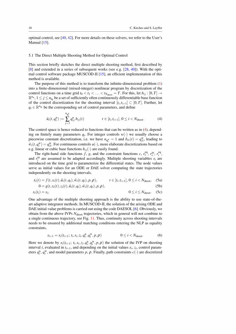
The purpose of this method is to transform the infinite-dimensional problem (1)into a finite-dimensional (mixed-integer) nonlinear program by discretization of thecontrol functions on a time grid t0 < t1 < .. . < tNshoot = T . For this, let bi j : [0,T ]→Rnu , 1≤ j≤ nqi be a set of sufficiently often continuously differentiable base functionof the control discretization for the shooting interval [ti, ti+1] ⊂ [0,T ]. Further, letqi ∈ Rnqi be the corresponding set of control parameters, and define

ui(t,qui ) :=

nqui

∑j=1

qui j bi j(t) t ∈ [ti, ti+1], 0≤ i < Nshoot. (4)

The control space is hence reduced to functions that can be written as in (4), depend-ing on finitely many parameters qi. For integer controls w(·) we usually choose apiecewise constant discretization, i.e. we have nqw

i= 1 and bi1(t) = qw

i1, leading towi(t,qw

i ) = qwi1. For continuous controls u(·), more elaborate discretizations based on

e.g. linear or cubic base functions bi j(·) are easily found.The right-hand side functions f , g, and the constraint functions c, req

c , rinc , req

i ,and rin

i are assumed to be adapted accordingly. Multiple shooting variables si areintroduced on the time grid to parameterize the differential states. The node valuesserve as initial values for an ODE or DAE solver computing the state trajectoriesindependently on the shooting intervals.

xi(t) = f (t,xi(t), ui(t,qi), wi(t,qi), p,ρ), t ∈ [ti, ti+1], 0≤ i < Nshoot, (5a)0 = g(t,xi(t),zi(t), ui(t,qi), wi(t,qi), p,ρ), (5b)

xi(ti) = si, 0≤ i≤ Nshoot. (5c)

One advantage of the multiple shooting approach is the ability to use state-of-the-art adaptive integrator methods. In MUSCOD-II, the solution of the arising ODE andDAE initial-value problems is carried out using the code DAESOL [6]. Obviously, weobtain from the above IVPs Nshoot trajectories, which in general will not combine toa single continuous trajectory, see Fig. 11. Thus, continuity across shooting intervalsneeds to be ensured by additional matching conditions entering the NLP as equalityconstraints,

si+1 = xi(ti+1; ti,si,zi,qui ,q

wi , p,ρ) 0≤ i < Nshoot. (6)

Here we denote by xi(ti+1; ti,si,zi,qui ,q

wi , p,ρ) the solution of the IVP on shooting

interval i, evaluated in ti+1, and depending on the initial values si, zi, control param-eters qu

i , qwi , and model parameters p, ρ . Finally, path constraints c(·) are discretized


on an appropriately chosen grid. To ease the notation, we assume in the followingthat all constraint grids match the shooting grid.

Fig. 11 A multiple shooting discretization in time. A constant initialization of state nodes si, 0≤ i≤ N isshown on the left, and a continuous solution after convergence on the right. Continuity is required in theoptimal solution only, ensured by matching conditions.

Structured Nonlinear Programming From this discretization and parameterizationresults a highly structured (MI)NLP of the form

minξC,ξI

Nshoot

∑i=0

Φi(si,zi, ui(ti,qu

i ), wi(ti,qwi ), p,ρ

)(7a)

s.t. 0 = xi(ti+1;si,zi,qui ,q

wi , p,ρ)− si+1, 0≤ i < Nshoot, (7b)

0 = g(ti,si,zi, ui(ti,qu


), 0≤ i≤ Nshoot, (7c)

0≤ c(ti,si,zi, ui(ti,qu


), 0≤ i≤ Nshoot, (7d)

0 = reqc(s0,sNshoot , p,ρ

), (7e)

0≤ rinc(s0,sNshoot , p,ρ

),

0 = reqi

(si,zi, ui(ti,qu


), 0≤ i≤ Nshoot, (7f)

0≤ rini(si,zi, ui(ti,qu


), 0≤ i≤ Nshoot,

qwi ∈Ωw, ρ ∈Ωρ , (7g)

where the vectors ξC, ξI shall contain all unknowns of the problem

ξC =(s0, . . . ,sNshoot ,q

u0, . . . ,q

uNshoot−1, p

), ξI =

(qw

0 , . . . ,qwNshoot−1,ρ

). (8)

For the ease of notation in (7d, 7f) we write

uNshoot(tNshoot ,qNshoot) := uNshoot−1(tNshoot ,qNshoot−1).

and analogously for w. We may then continue to solve this large-scale structured(MI)NLP using one of the solvers mentioned in the introduction. To be efficient,this usually requires extensive exploitation of the arising NLP structures. Possibleapproaches include e.g. SQP methods with block-wise high-rank updates of Hessianapproximations, partial reduction using the algebraic constraints to eliminate the zifrom the problem, and condensing algorithms for a reduction of the size of the arisingquadratic subproblems. For details, we refer to e.g. [8, 27, 28].


5.2 Sensitivity Computation and Automatic Derivatives

From the structured NLP (7) is becomes clear that AMPL objectives and most AMPLconstraints can be evaluated as usual, and this also holds true for gradients or Jaco-bians. The exception to this are ODE and DAE constraint functions as they do notdirectly enter (7). Evaluation of these functions occurs during solution and sensitiv-ity computation for the multiple shooting IVPs, carried out by an ODE/DAE solvercalled to evaluate the residual or a derivative of the matching constraint (7b).

We exemplarily consider the ODE case and look in more detail at the computa-tion of a directional derivative X ·d of differential state trajectory with respect to theproblem’s unknowns,

X =dx(ti+1; ti,si,zi,qi, p,ρ)

d(si,qi, p)∈ Rnx×(nx+nq+np) (9)

being the Jacobian of the solution of the IVP on [ti, ti+1] with respect to the unknowns(si,qi, pi) of the problem in the shooting node at ti. For a direction d = (ds,dq,p) ∈Rnx+nq+np this may e.g. be done by solving the system (10) of so-called variationaldifferential equations,

xd(t) = fx(t) · xd(t)+ fq,p(t) ·dq,p, t ∈ [ti, ti+1], (10a)xd(ti) = ds, (10b)

simultaneously and using the same scheme (e.g. choice of method, step sizes, orders,etc.) with the IVP itself. Basic calculus then shows xd(ti+1) = X · d. In (10), time-dependent Jacobians of the ODE constraint are denoted by

fx(t) =∂ f∂x

(t,x(t), u(t),w(t), p,ρ), fq,p(t) =∂ f

∂ (q, p)(t,x(t), u(t),w(t), p,ρ)

Much in the same spirit, directional derivatives of z(t) and derivatives into direc-tions containing the shooting node algebraic unknowns zi can be computed for partialreduction of DAE systems, see [27].

For direct multiple shooting NLPs, typically a significant amount of total theruntime, easily in excess of 80%, is spent on computing sensitivities of IVP solutions.Hence, it is vitally important to exploit the availability of automatic sparse derivativesof the ODE and DAE constraints in AMPL when computing fx and fq,p. Here, ourapproach of modeling dynamic constraints in AMPL has the additional advantage ofnot requiring a separate automatic differentiation tool, while at the same time beingfaster and more precise than finite difference approximations. In the MUSCOD-IIinterface to AMPL, we provide both dense and sparse Jacobians as well as directionalderivatives formed from sparse matrix-vector products to the DAE solver DAESOL.

5.3 MUSCOD-II Specific Solver Options and AMPL Suffixes

This section addresses the specification of shooting discretizations, of interpolatedinitial guesses, of scaling factors, and of slope constraints in AMPL models to besolved by MUSCOD-II.


Specifying a Discretization MUSCOD-II applies a multiple shooting discretizationin time to control trajectories, differential- and algebraic state trajectories, path con-straints, and Lagrange- and integral least-squares-type objectives, cf. [27]. The num-ber of multiple shooting intervals can be chosen using the solver option nshoot. Forpoint least-squares objectives as well as for point constraints, the MUSCOD-II back-end ensures the introduction of shooting nodes in the respective time points. Hence,the solver option nshoot specifies a minimum number of shooting intervals only.Moreover, adaptive refinement of the shooting discretization may be triggered byseveral mixed–integer strategies of the MS-MINTOC algorithms, cf. [40]. The finalnumber of shooting intervals used for computation of the optimal solution is availablefrom the solution file written by the frontend, see §4.4.

Initial Guesses, Scaling, and Slope Constraints For MUSCOD-II we provide severaladditional suffixes that allow to model more elaborate initializations, to apply scalefactors to variables, objective, and constraints, and to impose constraints on the slopeof linear or cubic spline controls.

interp_to Specifies a second initializer for a differential state at the end of the timehorizon. Let α be the initial guess and β be the value of suffix interp_to. Theinitialization of the state trajectory shall be a linear interpolation between the firstand the second initializer,

x(t) =T − t

Tα +

tT

β , t ∈ [0,T ]. (11)

Since AMPL does not provide a means of telling whether a suffix is uninitialized,and since interpreting β = 0 as uninitialized is not a viable option, the dedicatedsolver option s_spec has to be set in order to enable the interp_to. In this case,suffix interp_to has to be set for all differential state variables.

scale Specifies scale factors for variables, constraint, and objectives. The defaultvalue 0 means to infer the scale factor from the initial guess. If none is provided,a default scale factor of 1 is assumed.

slope_max and slope_min Specify upper and lower bounds on the slopes of piece-wise linear or cubic controls. Since AMPL does not allow for non-zero defaultvalues of suffices, this suffix must be set for all controls that are not of piecewiseconstant type.

Solver Options Solver options recognized by the MUSCOD-II backend comprise thefollowing keywords:

nshoot The minimum number of multiple shooting intervals to use. As already de-scribed above, constraint grids, point least-squares objective grids, and also MS-MINTOC strategies may increase this.

itmax The maximum number of SQP iterations allowed.atol The acceptable KKT tolerance for termination of the SQP solver.levmar Levenberg-Marquardt regularization for the Hessian of the Lagrangian.bflag The MS-MINTOC strategy code, see [40].


stiff Set to use the BDF-type solver DAESOL [6] which can cope with stiff DAEsystems. Unset to use a faster Runge-Kutta-Fehlberg–type method for non-stiffODEs.

deriv Set to sparse to use sparse Jacobians of the ODE/DAE provided by AMPL.Set to dense to use dense Jacobians of the ODE/DAE provided by AMPL. Setto finitediff to approximate derivatives by finite differences, ignoring AMPLderivatives.

solve Selects the globalization method for the SQP solver. Available methods in-clude solve_fullstep (no globalization), solve_slse (a line search method),and solve_tbox (a box-shaped trust region method).

hess Selects the Hessian approximation method to use. Available options includehess_const (constant Hessian), hess_update (a BFGS Hessian approxima-tion), hess_limitedmemoryupdate (a limited memory BFGS Hessian approx-imation), hess_gaussnewton (Gauß–Newton approximation of the Hessian),and hess_finitediff (finite difference exact Hessian).

Usage in AMPL Fig. 12 shows two lines of exemplary AMPL code that demonstratehow to load the MUSCOD-II solver and pass algorithmic options from an AMPLmodel file.

option solver muscod;option muscod_options "nshoot=20 atol=1e-8 itmax=200 hess=hess_gaussnewton";option muscod_auxfiles "rc";

Fig. 12 Exemplary AMPL code to load the MUSCOD-II solver and pass solver options and row andcolumn names.

6 Limitations and Possible Further Extensions

The extensions to the AMPL modeling language presented so far suffice to treat theclass (1) of mixed-integer DAE-constrained optimal control problems. However, anumber of possible extensions of this problem class are discussed next: Modeling offully implicit ODE and DAE systems of the form

0 = f (t,x(t), x(t),z(t),u(t),w(t), p,ρ) t ∈ [0,T ],0 = g(t,x(t),z(t),u(t),w(t), p,ρ),

or alternatively of a semi-implicit form which is preferred by many DAE solver im-plementations,

A(t,x(t),z(t),u(t),w(t), p,ρ)x(t) = f (t,x(t),z(t),u(t),w(t), p,ρ) t ∈ [0,T ],0 = g(t,x(t),z(t),u(t),w(t), p,ρ),

might be realized using a more sophisticated diff user function. As the current im-plementation of the AMPL solver library does not provide sufficient information to


associate x(t) arguments with x(t) arguments, this would require manipulation ofAMPL expression DAGs for all ODE constraints.

For convenience, the functionality of diff() could also be extended to allowhigher-order ODEs to be formulated by passing the differential’s order as a thirdargument, e.g. write diff(x,t,2) for x(t). This would further reduce the number oflines required for the presented COPS fluid flow problem of §3.1.

For some DAE problems, in order to promote sparsity, automatic introduction ofdefined variables as additional algebraic states might be preferred over the in-placeevaluation of defined variables that is currently carried out.

The use of non-smooth operators such as max, min, | · |, or conditional statementscould be allowed inside ODE constraints. This would open the possibility for mod-eling hybrid and implicitly switched systems in a quick and convenient way, givenan ODE and DAE capable of computing derivatives of switching ODEs’ solutions.The use of certain logical and non-smooth operators could also be allowed in pathand point constraints, leading e.g. to optimal control problems with complementarityconstraints [] or vanishing constraints [2]. citations

Certain optimal control problems of practical relevance require a multi–stagesetup. Here, the number of differential and/or algebraic states and the number of con-trols may change at a certain, possibly implicitly determined point in time. Modelingmulti–stage optimal control problems currently appears difficult using the extensionsdescribed in this report. Here AMPL’s syntax provides insufficient contextual infor-mation about the stage a certain variable or constraint should be assigned to.

7 Summary and Outlook

We described an extension to the AMPL modeling language that extends the applica-bility of the AMPL modeling language beyond the domain of MINLPs by allowingto conveniently model mixed-integer DAE-constrained optimal control problems inAMPL. Contrary to prior approaches at modeling such problems in AMPL by ex-plicitly encoding a discretization scheme for the dynamic parts of the model, ourapproach separates model equations and discretization scheme.

We showed that the proposed extensions do not require intrusive changes to theAMPL language standard or implementation itself, as they consist of a set of threeAMPL user functions and an AMPL suffix. The TACO toolkit for AMPL controloptimization was presented and serves as an interface between AMPL stub.nl filesand an optimal control code. TACO is open–source and designed to facilitate thecoupling of existing optimal control software packages to AMPL.

To demonstrate the applicability of TACO, we used this new toolkit to implementan AMPL interface for the optimal control software packages MUSCOD-II and itsmixed–integer optimal control extension MS-MINTOC.

The modeling and solution of two exemplary control problems in AMPL using theproposed extensions showed the benefits of the proposed approach, namely shortermodel code, improved readability, flexibility in the choice of a discretization scheme,and the possibility to adaptively modify and refine such a scheme.


In the future, it would be desirable to have implementations of a number of al-ternative schemes for evaluation of ODE and DAE constraints available, e.g. vari-ous collocation schemes. This would enable the immediate use of NLP and MINLPsolvers.

Acknowledgements The research leading to these results has received funding from the European UnionSeventh Framework Programme FP7/2007-2013 under grant agreement no FP7-ICT-2009-4 248940. Thefirst author acknowledges a travel grant by Heidelberg Graduate Academy, funded by the German Excel-lence Initiative. We thank Hans Georg Bock, Johannes P. Schlöder, and Sebastian Sager for permission touse the optimal control software package MUSCOD-II and the mixed–integer optimal control algorithmMS-MINTOC.

References

1. Abhishek K, Leyffer S, Linderoth T (2010) FilMINT: An Outer Approximation–Based Solver for Mixed–Integer Nonlinear Programs. INFORMS Journal onComputing 22(4):555–567

2. Achtziger W, Kanzow C (2008) Mathematical programs with vanishing con-straints: optimality conditions and constraint qualifications. Mathematical Pro-gramming Series A 114:69–99

3. Åkesson J, Årzén K, Gräfvert M, Bergdahl T, Tummescheit H (2008) Model-ing and optimization with Optimica and JModelica.org — Languages and toolsfor solving large-scale dynamic optimization problems. Computers & ChemicalEngineering 34(11):1737–1749

4. Albersmeyer J (2010) Adjoint based algorithms and numerical methods for sen-sitivity generation and optimization of large scale dynamic systems. PhD thesis,Ruprecht–Karls–Universität Heidelberg

5. Barton P, Pantelides C (1993) gPROMS — A Combined Discrete/ContinuousModelling Environment for Chemical Processing Systems. Simulation Series25:25–34

6. Bauer I, Bock H, Körkel S, Schlöder J (1999) Numerical Methods for InitialValue Problems and Derivative Generation for DAE Models with Application toOptimum Experimental Design of Chemical Processes. In: Scientific Computingin Chemical Engineering II, Springer, pp 282–289

7. Betts J, Eldersveld S, Huffman W (1993) Sparse nonlinear programming testproblems (Release 1.0). Tech. Rep. BCSTECH-93-074, Boeing Computer Ser-vices

8. Bock H, Plitt K (1984) A Multiple Shooting algorithm for direct solution of op-timal control problems. In: Proceedings of the 9th IFAC World Congress, Perga-mon Press, Budapest, pp 242–247

9. Bonami P, Biegler L, Conn A, Cornuéjols G, Grossmann I, Laird C, Lee J, LodiA, Margot F, Sawaya N, Wächter A (2005) An Algorithmic Framework For Con-vex Mixed Integer Nonlinear Programs. Research Report RC23771, IBM T.J.Watson Research Center

10. Box G, Hunter W, MacGregor J, Erjavec J (1973) Some problems associatedwith the analysis of multiresponse data. Technometrics 15:33—-51


11. Bryson A, Ho Y (1975) Applied Optimal Control: Optimization, Estimation, andControl. John Wiley & Sons

12. Cesari L (1983) Optimization — Theory and Applications. Springer Verlag13. Cuthrell J, Biegler L (1987) On the optimization of differential-algebraic process

systems. AIChE 33:1257–127014. Diehl M (2001) Real-Time Optimization for Large Scale Nonlinear Processes.

PhD thesis, Ruprecht–Karls–Universität Heidelberg15. Diehl M, Leineweber D, Schäfer A (2001) MUSCOD-II Users’ Manual. IWR

Preprint 2001-25, Interdisciplinary Center for Scientific Computing (IWR),Ruprecht–Karls–Universität Heidelberg, Im Neuenheimer Feld 368, 69120 Hei-delberg, Germany

16. Diehl M, Bock H, Kostina E (2006) An approximation technique for robust non-linear optimization. Mathematical Programming 107:213–230

17. Dolan E, Moré J, Munson T (2004) Benchmarking Optimization Software withCOPS 3.0. Tech. Rep. ANL/MCS-TM-273, Mathematics and Computer ScienceDivision, Argonne National Laboratory, 9700 South Cass Avenue, Argonne, IL60439, U.S.A.

18. Elmqvist H, Brück D (2001) Dymola — Dynamic Modeling Language. User’smanual, Dynasim AB

19. Fletcher R, Leyffer S (1999) User manual for filterSQP. Tech. rep., University ofDundee

20. Floudas C, Pardalos P, Adjiman C, Esposito W, Gumus Z, Harding S, Klepeis J,Meyer C, Schweiger C (1999) Handbook of Test Problems for Local and GlobalOptimization. Kluwer Academic Publishers

21. Fourer R, Gay D, Kernighan B (1990) A modeling language for mathematicalprogramming. Management Science 36:519–554

22. Gill P, Murray W, Saunders M (2002) SNOPT: An SQP Algorithm for large–scale constrained optimization. SIAM Journal on Optimization 12:979–1006

23. Gropp W, Moré J (1997) Optimization Environments and the NEOS Server. In:Buhmann M, Iserles A (eds) Approximation Theory and Optimization, Cam-bridge University Press, pp 167–182

24. Kameswaran S, Biegler L (2008) Advantages of nonlinear-programming-basedmethodologies for inequality path-constrained optimal control problems - a nu-merical study. SIAM Journal on Scientific Computing 30:957–981

25. Kühl P, Milewska A, Diehl M, Molga E, Bock H (2005) NMPC for runaway-safefed-batch reactors. In: Proc. Int. Workshop on Assessment and Future Directionsof NMPC, pp 467–474

26. Leineweber D (1995) Analyse und Restrukturierung eines Verfahrens zur di-rekten Lösung von Optimal-Steuerungsproblemen. Diploma thesis, Ruprecht–Karls–Universität Heidelberg

27. Leineweber D (1999) Efficient reduced SQP methods for the optimization ofchemical processes described by large sparse DAE models, Fortschritt-BerichteVDI Reihe 3, Verfahrenstechnik, vol 613. VDI Verlag, Düsseldorf

28. Leineweber D, Bauer I, Schäfer A, Bock H, Schlöder J (2003) An efficient mul-tiple shooting based reduced SQP strategy for large-scale dynamic process opti-mization (Parts I and II). Computers and Chemical Engineering 27:157–174


29. Logsdon J, Biegler L (1992) Decomposition strategies for large-scale dynamicoptimization problems. Chemical Engineering Science 47(4):851–864

30. Maria G (1989) An adaptive strategy for solving kinetic model concomitantestimation-reduction problems. Can J Chem Eng 67:825

31. Mattsson S, Elmqvist H, Broenink J (1997) Modelica: An International effortto design the next generation modelling language. Journal A, Benelux QuarterlyJournal on Automatic Control 38(3):16–19, special issue on Computer AidedControl System Design, CACSD, 1998.

32. Milewska A (2006) Modelling of batch and semibatch chemical reactors – safetyaspects. PhD thesis, Warsaw University of Technology

33. Moessner-Beigel M (1995) Optimale Steuerung für Industrieroboter unterBerücksichtigung der getriebebedingten Elastizität. Diploma thesis, Ruprecht–Karls–Universität Heidelberg

34. Nocedal J, Wright S (2006) Numerical Optimization, 2nd edn. Springer Verlag,Berlin Heidelberg New York

35. Petzold L, Li S, Cao Y, Serban R (2006) Sensitivity analysis of differential-algebraic equations and partial differential equations. Computers and ChemicalEngineering 30:1553–1559

36. Plitt K (1981) Ein superlinear konvergentes Mehrzielverfahren zur direktenBerechnung beschränkter optimaler Steuerungen. Diploma thesis, RheinischeFriedrich–Wilhelms–Universität Bonn

37. Potschka A, Bock H, Schlöder J (2009) A minima tracking variant of semi-infinite programming for the treatment of path constraints within direct solutionof optimal control problems. Optimization Methods and Software 24(2):237–252

38. Rothschild B, Sharov A, Kearsley A, Bondarenko A (1997) Estimating growthand mortality in stage-structured populations. Journal of Plankton Research19:1913––1928

39. Rutquist P, Edvall M (2010) PROPT — Matlab Optimal Control Software. User’smanual, TOMLAB Optimization

40. Sager S (2005) Numerical methods for mixed–integer optimal control problems.Der andere Verlag, Tönning, Lübeck, Marburg

41. Sager S (2011) A benchmark library of mixed-integer optimal control problems.In: Proceedings MINLP09, (accepted)

42. Sager S, Bock H, Diehl M (2011) The Integer Approximation Error inMixed-Integer Optimal Control. Mathematical Programming A DOI 10.1007/s10107-010-0405-3

43. von Stryk O (1999) User’s guide for DIRCOL (Version 2.1): A direct colloca-tion method for the numerical solution of optimal control problems. Tech. rep.,Technische Universität Müchen, Germany

44. Tjoa IB, Biegler L (1991) Simultaneous solution and optimization strategies forparameter estimation of differential-algebraic equations systems. Ind Eng ChemRes 30:376—-385

45. Wächter A, Biegler L (2006) On the Implementation of an Interior-Point FilterLine-Search Algorithm for Large-Scale Nonlinear Programming. MathematicalProgramming 106(1):25–57


Appendix

The following appendix sections contain supplementary material intended to guidesoftware developers interested in using the presented TACO toolkit to interface theiroptimal control codes with AMPL. Section A explains the most important data struc-tures that hold information about the mapping from the optimal control point of viewto the AMPL one. Section B lists functions available to optimal control codes forevaluating AMPL functions. Section C explains error codes emitted by the TACOtoolkit, and mentions possible remedies.

A TACO Data Structures Exposed to Optimal Control Problem Solvers

This sections lists TACO data structures exposed to developers of codes for solv-ing optimal control problems. We discuss several snippets taken from the header fileocp_frontend.h, which should be consulted for additional details.

A.1 Data Structures Mapping from AMPL to Optimal Control

The optimal control frontend provides a collection of fields that hold the optimalcontrol problem interpretation of every AMPL variable passed to the solver. They arelaid out as follows:

enum vartype_t vartype_AMPL_defined = -2, // AMPL "defined" variablevartype_unknown = -1, // type not yet knownvartype_t = 0, // independent variable ("time")vartype_x = 1, // differential state of an ODE/DAEvartype_z = 2, // algebraic state of a DAEvartype_u = 3, // control function to be discretizedvartype_p = 4, // global model parametervartype_tend = 5 // end time variable

;

enum vartype_t *vartypes; // OCP types assigned to AMPL variablesint *varindex; // OCP vector indices assigned to AMPL variables

The field vartypes gives the OCP variable type of an AMPL variable, i.e.,whether the variable is t, T , a component of vector p, or a component of one ofthe vector trajectories x, z, or u and w. For the case of it being a vector component,the field varindex holds the index into the OCP variable or trajectory vector. ForAMPL constraints and objectives, no mapping information from AMPL to the OCPperspective is provided.

A.2 Data Structures Mapping from Optimal Control to AMPL

The AMPL optimal control frontend provides a collection of structures holding theAMPL perspective for every component of an optimal control problem according toproblem class (1). Starting with information about problem dimensions, the followingvariables are provided and should be self-explanatory.


int nx; // number of differential statesint nz; // number of algebraic statesint nu; // number of control functionsint np; // number of model parametersint npc; // number of inequality path constraintsint ncc_eq; // number of coupled equality constraintsint ncc_in; // number of coupled inequality constraints

Information about both the independent time variable and the end-time variableis held in a structured variable named endtime of the following layout.

struct ocp_time_t int index; // AMPL index of the final time variable, or -1const char *name; // AMPL name of the final time variableint fixed; // flag indicating whether tf is fixed, index may be -1 thenreal init; // initial or fixed end time, even if idx_tf=-1real scale; // scale factor for tfreal lbnd; // lower bound for tfreal ubnd; // upper bound for tf

int idx_t; // AMPL index of the free time variable tconst char *name_t; // AMPL name of the free time variable

;

struct ocp_time_t endtime; // time horizon information

For a fixed-endtime scenario, endtime.index is −1, the field endtime.initholds the fixed end time. For a variable end-time scenario, endtime.index is non-negative and the field endtime.init holds the initial guess for the free end time ifavailable, and is set to 1.0 otherwise.

The following structured variable xstates holds information about differentialstate trajectory variables, and associated right hand side functions.

struct ocp_xstate_t int index; // AMPL index of differential state trajectory variableconst char *name; // AMPL name of the differential state trajectory variableint fixed; // AMPL index of initial value constraint, -1 if nonereal init[2]; // initializers at t=0 and t=tfreal scale; // scale factorreal lbnd; // lower boundreal ubnd; // upper bound

int ffcn_index; // AMPL index of ODE constraintconst char *ffcn_name; // AMPL name of ODE constraintreal ffcn_scale; // scale factorreal rhs_factor; // constant factor in front of diff()

;

struct ocp_xstate_t *xstates; // differential state trajectories information

Here, the field fixed holds the AMPL index of the initial value constraint forthis ODE state. It is −1 if the ODE state’s initial value is free. The initializer initprovides two values for linear interpolation (see suffix .interp_to).

The field ffcn_index holds the AMPL constraint index of the right hand sidefunction associated with a differential state. Even though we currently support ex-plicit ODEs only, AMPL-internal rearrangement of constraint expressions may causea negative sign on the diff() call. Hence the field rhs_factor is introduced tocompensate for AMPL-internal representations of the form −x(t) = f (t,x(t), . . .).

Similar to differential states, the structured variable zstates holds informationabout algebraic state trajectories.


struct ocp_zstate_t int index; // AMPL index of algebraic state trajectory variableconst char *name; // AMPL name of algebraic state trajectory variablereal init; // constant initial guess for algebraic state trajectoryreal scale; // scale factorreal lbnd; // lower boundreal ubnd; // upper bound

// we keep gfcn() information here as well, but keep in mind that the relation-// ship between z[] and gfcn() is fully implicit, i.e. no 1-1 correspondence!

int gfcn_index; // AMPL index of DAE constraintconst char *gfcn_name; // AMPL name of DAE constraintreal gfcn_scale; // scale factor for DAE constraint

;

struct ocp_zstate_t *zstates; // algebraic state trajectories information

It is important to keep in mind that DAE constraints are not associated with al-gebraic state trajectory variables by a one–one mapping. We merely keep both in thesame array for simplicity, as their numbers must match.

Information about integer and continuous control trajectories is kept in a struc-tured variable named controls with the following layout.

struct ocp_control_t int index; // AMPL indices of control trajectory variableconst char *name; // AMPL name of control trajectory variableint type; // control discretization typeint integer; // flag indicating integer controlsreal init; // initial guess for all control parameters on the horizonreal scale; // scale factor for controlreal lbnd; // lower bound for controlreal ubnd; // upper bound for control

// slope information for linear or cubic elementsreal slope_init; // initial guess for control slopereal slope_scale; // scale factor for control slopereal slope_lbnd; // lower bound for control slopereal slope_ubnd; // upper bound for control slope

;

struct ocp_control_t *controls; // control trajectories information

Herein, the field type denotes the (solver-dependent) discretization type to beapplied to this control trajectory The field integer is set to 1 if the control is abinary or integer control, and to 0 if it is a continuous control. For piecewise linearand piecewise cubic discretization types, additional information about slope limitsand initial guesses is provided.

Finally, model parameters information is provided in a structured variable namedparams, with layout as follows. This concludes AMPL variables information.

struct ocp_param_t int index; // AMPL indices of free model parametersconst char *name; // AMPL name of free model parametersreal init; // initial value for free parameterreal scale; // scale factors for free parameterreal lbnd; // lower bound for free parameterreal ubnd; // upper bound for free parameterint integer; // 1 if integer, 0 if real

;

struct ocp_param_t *params; // free parameters information


Information about Mayer-type, Lagrange-type, and integral least-squares-typeobjective functions (1a) is found in structured variables named mayer, lagrange,and clsq. Their layout is presented below.

struct ocp_objective_t int index; // AMPL index of objective functionconst char *name; // AMPL name of objective functionint dpnd; // dependency flags from enum vartype_tint maximize; // 1 for maximization, 0 for minimizationreal scale; // scale factor

// additional information for least-squares type objectivesint nparts; // number of residualsexpr **parts; // residual AMPL expressions

;

struct ocp_objective_t mayer; // Mayer type objective function informationstruct ocp_objective_t lagrange; // Lagrange type objective function informationstruct ocp_objective_t clsq; // Integral least-squares type objective information

Herein, dpnd is a bit field with bit k (k ≥ 0) set if and only if the objective func-tion’s AMPL expression depends on an AMPL variable with vartypes entry set tovalue k (see enum vartype_t). This allows for quick dependency checks that maysave run time e.g. in derivative approximation. The field maximize is set to 1 if theobjective function is to be maximized, and to 0 if it is to be minimized. Note thatleast-squares functions are recognized only if they are to be minimized. The fieldsnparts and parts hold information about the AMPL expression DAGs associatedwith the individual least-squares residual expressions of a least-squares objective.

Path constraints (1d) and coupled constraints (1e) information is held in structuredvariables named pathcon, cpcon_eq, and cpcon_in with the following layout.

struct ocp_constraint_t int index; // AMPL index of constraintconst char *name; // AMPL name of constraintint side; // side of inequality constraint (0=lower, 1=upper)int dpnd; // dependency flags from enum vartype_treal scale; // scale factor

;

struct ocp_constraint_t *pathcon; // inequality path constraintsstruct ocp_constraint_t *cpcon_eq; // coupled equality constraintsstruct ocp_constraint_t *cpcon_in; // coupled inequality constraints

Path constraints (1d) always are inequality constraints. For coupled constraints (1e),equality and inequality constraints are stored in separate arrays. For two-sided in-equality constraints l ≤ c(x)≤ u, the field side indicates which side of the constraintshould be evaluated.

Information about decoupled point constraints (1f) and point least-squares ob-jectives (1a) is stored in a structured variable named grid. For each objective orconstraint evaluation time, a grid node is introduced and holds information about theassociated objective or constraint. Grid nodes are guaranteed to be unique, i.e. notwo nodes share the same time point, and are sorted in ascending order. The grid isguaranteed to contain at least two nodes: The first grid node will always be at time 0,and the last grid node will always be at time tf.

struct ocp_grid_node_t int n_eq; // number of equality point constraints


struct ocp_constraint_t *con_eq; // equality point constraint informationint n_in; // number of inequality point constraintsstruct ocp_constraint_t *con_in; // inequality point constraint informationint ncc_eq; // number of equality coupled constraintsint *ccidx_eq; // indices of equality coupled constraintsint ncc_in; // number of inequality coupled constraintsint *ccidx_in; // indices of inequality coupled constraintsstruct ocp_objective_t lsq; // node least-squares objective information

;

struct ocp_grid_t int n_nodes; // number of grid nodesreal *times; // it’s more practical to have the times herestruct ocp_grid_node_t *nodes; // information about what is on a grid node

;

struct ocp_grid_t grid; // constraint and node-least-squares grid information

For equality and inequality point constraints (1f) on a grid node, the fields n_eqand n_in hold the dimensions and the fields con_eq and con_in the constraint in-formation, respectively. For coupled constraints (1e), we do not store pointers to con-straint information structures, but rather indices into the global lists cpcon_eq andcpcon_in. For solvers requiring linear separability of coupled constraints, this lay-out eases the setup of the coupled constraints’ block structure. Finally, the field lsqholds information about the point least-squares objective contribution in a node; againindex −1 indicates that no point least-squares objective is present.

B TACO Functions Exposed to Optimal Control Problem Solvers

This sections lists TACO functions exposed to developers of codes for solving opti-mal control problems.

Reading of the AMPL Model For reading and verifying the AMPL mode as well ascreation of management of the database the optimal control frontend provides thefollowing functions:

allocate_mappings allocates memory for the database to be created, prior to read-ing the stub.nl file provided by AMPL.

read_mappings calls the AMPL solver library to read the stub.nl file. Afterwards,the DAGs of all AMPL objectives and constraints are examined for appearanceof variables, calls to user functions, and nonsmooth operators. The role of AMPLvariables, constraints, and objectives in (1) is determined, and the database isfilled with appropriate information.

free_mappings frees memory allocated for the database after the optimal controlproblem has been solved.

A developer wishing to interface his optimal control problem solver with AMPLis provided with a number of functions that infer the optimal control problem’s struc-ture from a stub.nl file. The following listing shows a framework that could serve asa starting point for development of a solver interface.

// allocate memory for the "fg" reader of AMPL stub filesASL_alloc (ASL_read_fg);


asl->i.want_xpi0_ = 1; // indicate that we want the initial guessesasl->p.need_funcadd_ = 1; // indicate that we need to add user functions

// get AMPL stub file name and allocate memory for AMPL data structuresnl_name = getstub (&argv, &Oinfo);nl = jac0dim (nl_name, (fint) strlen (nl_name));if (nl == NULL)

error_out (error_readfile, nl_name);

// declare AMPL OCP frontend suffixesdeclare_suffixes ();

// read AMPL stub fileif (fg_read(nl, ASL_return_read_err|ASL_findgroups) != 0)

error_out (error_readfile, nl_name);

Oinfo.option_echo &= ~ASL_OI_echo; // don’t echo optionsOinfo.option_echo |= ASL_OI_badvalue; // but report bad option values

// read solver optionsif (getopts(&xargv[3], &Oinfo))

error_out (error_solverOptions);

allocate_mappings (); // allocate memory of AMPL OCP frontend dataread_mappings (); // infer OCP structure from AMPL stub file

// call optimal control problem solver here// use frontend information to set up problem and evaluate problem functions

free_mappings (); // free memory of AMPL OCP frontend data

Evaluating Problem Functions Once the database has been successfully filled withthe optimal control problem representation of the AMPL model, an appropriate opti-mal control problem solver can be called. This solver will have to evaluate problemfunctions. For conveniently doing so, the optimal control frontend provides a set offunctions that wrap around the conival and objival functions provided by AMPL’ssolver library:

evaluate_ode_rhs(i,y) evaluates the ODE right hand side xi(t) = fi(·) for a dif-ferential state xi(t), 0 ≤ i < nx. The vector y here is the plain vector of currentAMPL variable values.

evaluate_dae_rhs(i,y) evaluates the residual of DAE constraint gi(·), 0 ≤ i <nz.

evaluate_scaled_mayer(y) evaluates and scales the value of the Mayer objectiveterm, if a Mayer term exists.

evaluate_scaled_lagrange(y) evaluates and scales the value of the Lagrangeobjective term’s integrand, if a Lagrange objective exists.

evaluate_scaled_clsq(y,res) evaluates and scales the value of the Lagrangeobjective term’s integrand, if the integrand has least-squares structure and if aLagrange objective exists. Upon return the vector res holds the least-squaresresiduals, i.e. the individual values of each squared summand.

evaluate_scaled_node_lsq(n,y,res) evaluates one summand of a point least-squares objective term, if one exists. The integer n specified the number 0 < n <Nlsq of the measurement point to be evaluated.

evaluate_path_con(i,y) evaluates and scales the residual of an inequality pathconstraint.


evaluate_coupled_eq_con(i,y) evaluates and scales the residual of a coupledequality constraint.

evaluate_coupled_ineq_con(i,y) evaluates and scales the residual of a cou-pled inequality constraint.

evaluate_point_eq_con(n,i,y) evaluates and scales the residual of an equalitypoint constraint.

evaluate_point_ineq_con(n,i,y) evaluates and scales the residual of an in-equality point constraint.

Writing Solutions from a Solver For writing a solution file of the proposed format,the optimal control frontend provides three function calls to be used by a backendinterfacing an optimal control problem solver with AMPL:

alloc_solution allocates a solution structure given a discretization grid length.write_solution writes a solution file according to the proposed format and fills it

with the solution data found in the solution structure. The solver backend shouldhave queried the solver itself for this solution and copied it over to this solutionstructure.

free_solution free a previously allocated solution structure after it has been writ-ten to a solution file.

C TACO Toolkit Error Messages

This section lists all possible error messages emitted by the TACO toolkit duringanalysis and verification of the optimal control problem structure. If option solver-name_auxfiles is set to contain the characters “r” and “c”, error messages willshow the name of the offending variable, objective, or constraint.

1. to 5. are reserved for internal errors.6. “AMPL error reading stub.nl file filename”. AMPL could not read the

stub.nl file.7. “AMPL error getting solver options”. AMPL could not read the solver

options. Make sure your solver options string contains known keywords and validvalues only.

8. “I/O error writing solution file filename”. AMPL could not write thesolution file. Make sure that the current working directory is writeable and thatthe volume is not full.

9. “AMPL network variables are not supported”. The AMPL model con-tains network variables. Network modelling is currently not supported.

10. “AMPL piecewise linear terms are not supported”. The AMPL modelcontains piecewise linear terms. Nonsmooth models are currently not supported.

11. “diff() must be called exactly once for each differentialstate variable”.You called diff() more than once for the same variable. Every differential statevariable is associated with exactly one right hand side function, tough. Mostlikely, this is a typo in your model.


12. “Logical operator operator not permitted”. The shown constraint or ob-jective make use of a logical operator. Nonsmooth models are currently not sup-ported.

13. “Relational operator operator not permitted”. The shown constraint orobjective make use of a relational operator. Nonsmooth models are currently notsupported.

14. “Nonsmooth operator operator not permitted”. The shown constraint orobjective make use of a nonsmooth operator. Nonsmooth models are currentlynot supported.

15. “ODE constraints must be equality constraints”. You called diff()in an inequality constraint. All ODE constraints must be equality constraints,though.

16. “Cannot determine type of objective functions”. The shown object-ive cannot be determined to be of Mayer, Lagrange, integral least-squares, orpoint least-squares type. Please refer to Section 2.3 to learn about the structure ofsupported objective functions.

17. “Mayer objective function must not depend on controls”. The indi-cated objective is of Mayer type, and hence must not depend on control trajectoryvariables.

18. “The number of DAE constraints does not match the apparentnumber of algebraic variables”. The number of DAE constraints found inyour model does not match the number of algebraic variables you have declaredby letting suffix .type to value "dae". Make sure you’ve set the suffix of allalgebraic state variables, and make sure all your DAE constraints are equalityconstraints.

19. “Invalid value for suffix .type”. A variable, constraint, or objective hassuffix .type set to an unrecognized value. This should not happen unless you’reusing an incompatible OptimalControl.mod file.

20. “Missing independent time variable or end time variable”. TACOcould not determine which AMPL variables represent independent time or endtime. Make sure that the independent time variable appears as second argumentto all diff() calls, and that the end-time variable appears as second argument tointegral() in Lagrange-type objectives, or to eval() in Mayer-type objectivesor end-point constraints. If your AMPL model uses a time horizon of fixed length,make sure the end-time value shows up consistently in these places.

21. “Nesting a call to function name inside another is notallowed”. You nested two calls to functions diff(), eval(), or integral().This should never be necessary.

22. “As of now, diff() must be explicit. Try to write your ODE asdiff(var, t) = ...;”. The AMPL optimal control frontend currently sup-ported explicit ODEs only, i.e. the permitted formulation is x(t) = f (t,x(t), . . .)instead of the more general 0 = f (t,x(t), x(t), . . .). Try to rewrite your model touse explicit ODEs only.

23. “First argument to eval() must not be a constant”. The shown con-straint or objective calls eval() with two constant arguments. This is not sensi-ble. Either remove the calls to eval(), or make sure the expression to be eval-


uated references independent time or at least one state or control trajectory vari-able.

24. “Second argument to eval() must be >= 0.0, or the final timevariable”. The shown constraint or objective calls eval() with a time pointthat a) evaluates to a negative value, or b) is not a simple constant and not theend-time variable.

25. “First argument to integral() must not be a constant”. An objec-tive calls integral() with two constant arguments. This is not sensible. Eitherremove the call to integral(), or make sure the expression to be integratedreferences independent time or at least one state or control trajectory variable.

26. “Second argument to integral() must be the final timevariable”. The second argument of a call to integral() must be the final timevariable, or the final time itself.

27. “Second argument to diff() must be the independent timevariable”. The second argument of a call to diff() must be the independenttime variable.

28. “Function diff() expects differential state variable andindependent time variable as arguments”. The first argument to diffmust be a differential state trajectory variable, and the second argument of a callto diff() must be the independent time variable.

29. “Calls to integral() not allowed in constraints”. The function in-tegral() was called inside a constraint expression. Calls to integral() areonly allowed in a Lagrange-type or integral least-squares-type objective.

30. “Function call to name must enclose entire expression”. Calls toeval() and integral() must enclose the entire expression to be evaluated orintegrated.

31. “Only controls or parameters can be binary/integer variables”.AMPL’s binary or integer restriction may be applied to control trajectory vari-ables and model parameter variables only. Time as well as differential and alge-braic state trajectory variables must be continuous.

32. “Invalid grid node position, must be within [0,1] (tf free)or [0,tf] (tf fixed)”. A call to eval() used an invalid evaluation time.Allowed times are constants 0 to 1, being relative times on the time horizon [0, tf]if tf is free, absolute times 0 to tf if tf is fixed, or the end-time variable tf itself.

33. “Duplicate objective of name-type”. At most one objective of Mayer-,Lagrange-, and least-squares type is allowed per problem.

34. “Calls to eval() not allowed in ODE constraints”. The functioneval() was called inside an ODE constraint expression. This is not allowed.

35. “Calls to diff() not allowed in objective functions”. Thefunction diff() was called inside an objective function expression. This is notallowed.

Keywords Mixed-Integer Optimal Control, Differential ... C. Kirches and S. Leyffer Mathematical...

Documents

Transcript of Keywords Mixed-Integer Optimal Control, Differential ... C. Kirches and S. Leyffer Mathematical...