Flechsig 1

Implementation of a

Kalman Filter in LabVIEW

Evan Flechsig

CEN 4935 – Senior Software Engineering Project – Dr. Janusz Zalewski

U.A. Whitaker School of Engineering - Florida Gulf Coast University

April 11, 2010

Flechsig 2

1. Introduction

A Kalman Filter is a theoretical device that observes measurements over time that

contains noise and produces values that tend to be closer to the true values of the measurement. It

does this by applying a weight to a measurement which will be high for measurements with low

uncertainty and low for measurements with high uncertainty[1]

. There is extensive literature on

this topic.

Before using a Kalman Filter, the behavior of the system that we are measuring must be

described by a linear system [2][4][6]

. A linear system is described by these two equations: State

equation and Output equation. The State equation and Output equation are

In these equations, is the state of the system; is the measured output; is the time

index; is the known state of the system; and are the process and measurement noise

respectively; and are matrices that give value to their related term.

Once the linear system is defined, we must define the process noise and measurement

noise covariance. Being that noise are random, we must tell the filter how we expect this

noise to change, that is, what are the statistical properties of noise. Once these are defined, we

can look at the filter equations. For the linear system described above, the Kalman Filter

equations are as follows:

Flechsig 3

(1)

(2)

(3)

Equation number one is the Kalman Gain equation, number two is the state estimate

equation, and number three is the estimate error covariance equation. In equation number two,

there are two terms:

The first term represents what the state of the system would be if we didn’t have a measurement.

This means that we are assuming the system is acting just as the system model defines. The

second term of equation two is called the correction term, where it uses the Kalman Gain to

correct the assumed state due to our measurement. In equation number one, it’s generating a

value for the Kalman Gain. If the measurement noise is large, K will have a small value and will

not give much weight to the measurement in the estimation of the state. If the measurement noise

is small, K will be large and the measurement will be giving large weight when estimating the

state. [4]

2. Sine Wave Noise Example

The first example is running a Kalman Filter in LabVIEW that removes Gaussian noise

from a signal that replicates a sine wave. The block diagram for this virtual instrument can be

seen in Figure 2.1. Matrix A, B, and C define the state-space model and can be found in the red

square labeled “1”. In this example, the matrices are as follows:

Flechsig 4

How to obtain the A, B, and C matrices will be explained more in the next example. D is

left as all zeros because the inputs and the outputs have no relation. Next the auto covariance

matrices of the process noise (Q) and the measurement noise (R) must be defined for the Kalman

Gain seen in the purple box labeled “3”. They are used to determine how the process and

measurement noise change from one time interval to the next and are defined using the three

knobs on the front panel. We now have the inputs required to generate a Kalman Gain seen in the

green box labeled “5”. This is passed to a multiple state estimator seen in the blue box labeled

“4” which is set to accept a system with noise along with the state-space model.

Near the bottom middle of the block diagram in a yellow box labeled “2”, there are three

Gaussian noise generators along with two sine generators. The three noise generators take the

integer 400 as an input, which is the number of samples of the Gaussian noise pattern. The noise

generators also need to have a standard deviation defined. The first, second, and third noise

generator use , , and

respectively for their standard deviation. The two sine waves both

take 5 as their amplitude. To differentiate between the two waves, one is given a phase of 90°.

Now both the estimated model and the inputs with noise go into a state-space linear

simulator seen to the right of the yellow box. This then outputs out to a state trajectory graph.

Flechsig 5

Figure 2.1 – Block diagram of first Kalman Filter implementation

Figure 2.2 shows the outputted trajectory graph that is generated by both sine waves and

their corrected estimates after filtering the noise. It is difficult to see the corrections from the

filter; however you can see the corrections in Figure 2.3 that shows a section to a larger scale.

The darker blue is the model with noise while the lighter blue is the model after filtering.

Figure 2.2 – Output from sine wave Kalman Filter implementation

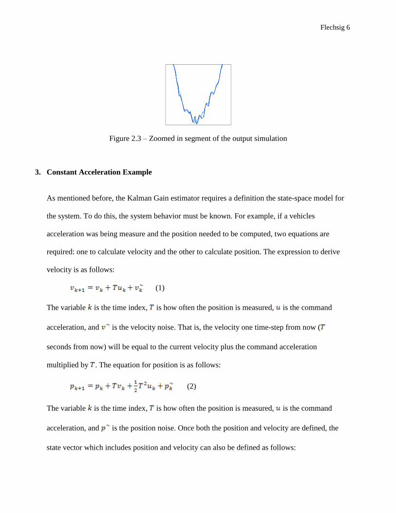
Flechsig 6

Figure 2.3 – Zoomed in segment of the output simulation

3. Constant Acceleration Example

As mentioned before, the Kalman Gain estimator requires a definition the state-space model for

the system. To do this, the system behavior must be known. For example, if a vehicles

acceleration was being measure and the position needed to be computed, two equations are

required: one to calculate velocity and the other to calculate position. The expression to derive

velocity is as follows:

(1)

The variable is the time index, is how often the position is measured, is the command

acceleration, and is the velocity noise. That is, the velocity one time-step from now (

seconds from now) will be equal to the current velocity plus the command acceleration

multiplied by . The equation for position is as follows:

(2)

The variable is the time index, is how often the position is measured, is the command

acceleration, and is the position noise. Once both the position and velocity are defined, the

state vector which includes position and velocity can also be defined as follows:

Flechsig 7

Now the linear state equation can be consolidated as follows:

The linear output equation can also be written as follows:

The matrix seen above as C is a relation that specifies the relationship between the

outputs and the states.

When both input and output equations have been defined, the matrices describing the

system are inputted on the front panel of the virtual instrument in LabVIEW. The filter should

consider the measurement every half second, so is equal to .5. Therefore, once substituting T,

we can calculate matrix A and matrix B. Matrix G is used to describe the relationship between

the process noise vector and the model states and remains the same from the previous example.

Matrix D is kept as all zeros because there is no transmission between the input and the output in

this case. After these conclusions, we have the following values:

Flechsig 8

The three knobs seen in the red box labeled “1” in Figure 3.4 are used to define the

process noise (State 1 & 2 Noise Variance) and the measurement noise (Output Noise variance).

They are knobs because they can be changed during the simulation. The matrices are defined in

the blue box labeled “2”. The output of the linear simulation is seen in the green box labeled “3”.

Figure 3.4 – The Front Panel of the Car Acceleration-Position simulation

The input that is being simulated is constant acceleration, meaning, a constant input. To

simulate this input, I’ve defined an array of 1’s in used this as an input for the Linear Simulation

module. This can be seen in the block diagram shown in Figure 3.5 in the red box labeled

“1”.These acceleration readings are also injected with Gaussian noise using a logical AND

operator seen in the blue box labeled “2”. The Linear Simulation module takes the estimated

model and these inputs, and graphs them on a State Trajectory Graph as seen in Figure 9.4. The

lines curve us, which is consistent with the position of an object with constant acceleration over

time.

Flechsig 9

Figure 3.5 – Block Diagram of Kalman Filter simulation of constant acceleration

A close up of the trajectory graph can be seen in Figure 3.6. The dark blue and Red lines

represent two different instances of the constant acceleration. The light blue and the gray lines

represent the filers estimate of the dark blue and red’s behavior respectively.

Figure 3.6 – State trajectory graph of the constant acceleration simulation

Flechsig 10

The difference may be difficult to see, so there is a blown version of the graph as Figure 3.7.

This cut is from 2.6(s) to 4.6(s)

.

Figure 3.7 – Segment of constant acceleration simulation

4. Conclusion

The Kalman Filter is a very strong tool to use when filtering out noise in a signal. Once

you’ve defined how the system is supposed to work, being able to define whether or not the next

measurement should have high or low weight is very valuable. Its application is not limited to

simple signals either. It can be expanded to use in CMOS sensors used for capturing light and

generating pictures or even sensing changes on a blog[5]

.

Future work for this project would include application of the filter behind an actual

sensor. The Kalman Filter was initially developed for aeronautical flight, so perhaps this could

be used to filter out noise from the altimeter in a satellite. It could also be used to filter out noise

from a temperature or moister sensor that is taking readings in remote locations. It would be

Flechsig 11

helpful to have these values filtered because unexpected noise is likely when dealing with remote

sensors in environments that aren’t controlled.

Flechsig 12

Appendix. Instructions for Using a Kalman Filter in LabVIEW.

0. Before starting, you need to know how to describe your linear system. For an

explanation, see Kalman Filter in LabVIEW section 9.0 and 9.2.[3]

1. Launch LabVIEW (these instructions are based on LabVIEW 8.5).

2. Open the VI which is an example that should be in the installation directory for

LabVIEW. Be default, it is “C:\Program Files\National

Instruments\LabVIEW 8.5\examples\Control Design\Getting

Started\State-Space Synthesis\CDEx Kalman Filter.vi”. Open this VI. It

may take some time to load because some dependencies also have to be loaded.

Flechsig 13

3. Once loaded, you should see a window similar to the one shown in Figure 1. This is the

front panel to the virtual instrument and is where you enter values for your variables.

Enter the matrices A, B, C, D and G into their respective boxes located near the top left

of the VI.

Figure 1 – Front Panel of the default Kalman Filter example.

4. Once these matrices are defined properly, open up the Block Diagram by going to

Window > Show Block Diagram.

Flechsig 14

5. You should then see a block diagram shown in Figure 2. Once here, you’ll need to

change the read inputs of the system which are the sine wave generators located in the red

box labeled “1”. This means that the Kalman device is filtering out noise from two of

sine waves. If you mouse over the yellow wire coming out of the sine wave generators,

you’ll see in the Context Help window1 that it’s outputting a 1-D array of doubles. The

waves are supposed to deliver the data to the linear simulator, which produces the system

outputs (both the actual disturbed by noise and filtered).

Figure 2 - Default Kalman Filter Block Diagram

6. The three blocks above the sine wave generators shown in Figure 2 are the Gaussian

noise generators. They will not be necessary for real work input because the data sets

already theoretically have noise in them. For the purposes of this demonstration, we’ll be

inputting an array of 1’s to represent constant acceleration. Right click in a white space

1 The Context Help window can be brought up by clicking on the yellow question mark that appears in the right

upper corner of the Block Diagram or Front Panel.

Flechsig 15

where you want to array to be on the block diagram and select Programming > Array >

Array constant. Then, fill the newly generated box with a double variable and make the

array all 1’s. Delete the two sine wave generators and wire your array to both of the AND

operators shown on the right side of the blue box labeled 2 in Figure 3. Then change the

number of samples in the Gaussian noise generator from 400 to the length of your double

array. This reconfiguration of the block diagram is shown in Figure 3.

Figure 3 – Block diagram after modifications

7. Once you have your input, return to the front panel of the VI and click the Run-Once

button under the “View” item in the tool bar. This will begin the simulation of your

system. Being that the body of this VI is within a while loop, the filter is going to run

continuously for many instances of the input and output the results on the graph. If your

data include the noise, your graph will not change as the noise will remain the same for

the same set of data points. In this example, I keep the Gaussian noise (represented in the

blue box labeled 2 in Figure 3), which is random and is generated for every iteration of

the while loop.

Flechsig 16

Figure 4 shows the output, which is the position of the system with respect to time. The

shape of the curve confirms the theory, because the position is a quadratic function of

time (see equation 1 on page 6)

Figure 4 - Constant acceleration filtered after noise

References

[1] G. Welch and G. Bishop, An Introduction to the Kalman Filter. North Carolina:

University of North Carolina at Chapel Hill, 2006.

[2] D. Hatfield, Fault Detection Using the Kalman Filter. Florida Gulf Coast

University. 2008.

[3] E. Flechsig, Kalman Filter in LabVIEW. Florida Gulf Coast University. April 6,

2010

[4] D. Simon, Kalman Filtering. Embedded Systems Programming. June 2001.

[5] P. Bogan, J. Johnston, U. Karadkar, R. Furuta, F. Shipman¸ Application of

Kalman Filters to Identify Unexpected Change in Blogs. Texas A&M

University.2008.

[6] D. Simon, Optimal State Estimation – Kalman, H∞, and Non linear Approaches.

Wiley-Interscience. June 23, 2006