JBM - pu.edu.np
87
JBM | Volume V| Issue I | December 2018 Volume V December 2018 Number 1 Editor-in-Chief Rabindra Ghimire Editorial Board Members Deepak Raj Paudel Surya Bahadur G.C. Umesh Singh Yadav Advisory Board Prof. Kundan Dutta Koirala, PhD Prof. Prem Raj Pant, PhD Prof. Puskar Bajracharya, PhD Prof. Radhe Shyam Pradhan, PhD Prof. Rajan Bahadur Poudel, PhD Published By School of Business Faculty of Management Studies Pokhara University Nepal www.pu.edu.np J BM The Journal of Business and Management
Transcript of JBM - pu.edu.np

JBM | Volume V| Issue I | December 2018
Volume V December 2018 Number 1
Editor-in-Chief
Rabindra Ghimire
Editorial Board Members
Deepak Raj PaudelSurya Bahadur G.C.Umesh Singh Yadav
Advisory Board
Prof. Kundan Dutta Koirala, PhDProf. Prem Raj Pant, PhD
Prof. Puskar Bajracharya, PhDProf. Radhe Shyam Pradhan, PhDProf. Rajan Bahadur Poudel, PhD
Published By
School of Business Faculty of Management Studies
Pokhara UniversityNepal
www.pu.edu.np
JBMThe Journal of Business and Management

Volume V December 2018 Number 1
AUTHORS IN THIS ISSUE
Bal Ram Bhattarai, Associate Professor, School of Business, Pokhara University. Email:
Bishow Raj Parajuli, Lecturer, School of Business, Pokhara University. Email: bishworajparajili@
gmail.com
Dipendra Karki, PhD Scholar, Kathmandu University, School of Management. Email: 1610002_
Hanuman Prasad, Professor, Faculty of Management, MLSU India. Email: profhanumanprasad@
gmail.com
Indira Shrestha, Lecturer, Tribhuvan University. Email: [email protected]
Kripa Kunwar, Lecturer, School of Business, Pokhara University. Email: [email protected]
Nguyen Viet Khoi, Professor VNU University of Economics and Business, Hanoi, Vietnam. Email:
Nirajan Bam, Lecturer, School of Business, Pokhara University, Nepal. Email: [email protected]
Rajesh Kumar Thagurathi, Associate Professor, School of Engineering, Pokhara University.
Email: [email protected]
Ravindra Prasad Baral, Lecturer, School of Business, Pokhara University. Email:
Santosh Kumar Gurung, Lecturer, School of Business, Pokhara University. Email: santoshgrg@
pu.edu.np
Shanti Devi Chhetri, Lecturer, School of Business, Pokhara University. Email: schhetri635@gmail.
com
Shashi Kant Chaudhary, Assistant Professor, British University Vietnam, Hanoi, Vietnam. Email:
JBMThe Journal of Business and Management
Volume V December 2018 Number 1
ARTICLES
An Empirical Analysis of Export-Led Growth of Vietnam: Trade in Value Added (TiVA) Approach 1
Nguyen Viet Khoi, Shashi Kant Chaudhary
The Dynamic Relationship between Tourism and Economy: Evidence from Nepal 16
Dipendra Karki
Digital Financial Literacy: A Study of Households of Udaipur 23
Hanuman Prasad , Devendra Meghwal, Vijay Dayama
Market Structure and Performance of Commercial Banks: Empirical Evidence from Nepal 33
Kripa Kunwar
Stock Price Behavior of Nepalese Commercial Banks: Random Walk Hypothesis 42
Nirajan Bam, Rajesh Kumar Thagurathi, Bipin Shrestha
Socio-Cultural, Economic and Environmental Impact of Tibetan Refugee Settlement on Host Community in Pokhara 53
Santosh Kumar Gurung, Bal Ram Bhattarai, Shanti Devi Chhetri, Anisha Bataju, Ganga Ghale
Event Study of Effect of Merger Announcement on Stock Price in Nepal 64
Shanti Devi Chhetri, Ravindra Prasad Baral
Influence of Demographic Factors on Job Satisfaction of Financial Institutions Workforce of Nepal 74
Indira Shrestha
The Semiotics of Contemporary Visual Texts: A Study in New Rhetorical Analysis 80
Bishwo Raj Parajuli
JBMThe Journal of Business and Management

JBMVolume V | Issue I | December 2018The Journal of Business and Management
1
An Empirical Analysis of Export-Led Growth of Vietnam: Trade in Value Added (TiVA) Approach
Nguyen Viet Khoi1, Shashi Kant Chaudhary2
Abstract
This paper examines the long-run relationship between domestic value added exports and economic growth of Vietnam using ARDL bounds test of cointegration on annual data covering the period of 1995-2014.The bounds test establishes existence of both short-run and long-run relationship between exports and GDP of Vietnam and shows a substantial contribution of exports in the real GDP (0.73 percent for one percent changes in the domestic value added exports). The exports pattern of Vietnam portrays it following the footsteps of export-led growth model of Mexico, whereby it has turned itself into export production platforms for MNCs by suppressing the wages, rather than developing own indigenous industrial capacity. In such scenario, it seems challenging for Vietnam to sustain its export-led growth which it has achieved so far based on its cheap labour. With the rising living standards, ultimately the comparative advantages of cheap labour force would vanish in the future, which will cause a wave of assembly jobs to flow out of Vietnam. Moreover, two other low-cost countries in the region, Cambodia and Myanmar are likely to rise as close competitors of Vietnam in the low cost assembly works in the near future. By that time, in case Vietnam fails to enter into higher value added activities, it will drag itself into the ‘middle income trap’. Therefore, the ‘assembly strategy’ shall be bonded with strategy to develop own indigenous industrial capacity, and national technological base. These will help Vietnam to upgrade its activities along value chains in forms of product upgrading, process upgrading, functional upgrading, and sectoral upgrading so that it can switch its role of ‘assembling agent’ to ‘indigenous producer’.
Keywords: ARDL, Breakpoint Unit Root, Exports-led Growth, Value Added Export, Vietnam
1. Introduction Export-led growth is a ‘development strategy’ that postulates that export expansion is a key factor for the economic growth of a nation. In theory, the expansion of exports can spur economic growth through several channels viz. (i) allocation of resources to the competitive sectors that results into increase in efficiency of the economy, (ii) generating employment opportunities to the unskilled labourers and improve equality, and (iii) greater inflows of FDI and technology transfers to the economy. The history of development of Germany and Japan in 1950s and 1960s; Mexico in 1970s; Asian Four Tigers (South Korea, Hong Kong, Taiwan,
and Singapore), in 1980s adopting export-led growth strategies is remarkable. There are a lot of empirical works done that support the export-led economic growth hypothesis, some of these significant works are Krueger (1978), Chenery (1979), Tyler (1981), Kavoussi (1984), Balassa (1985), Chow (1987), Fosu (1990), Salvatore and Hatcher (1991) etc. In contrary to it, there are some other empirical works viz. Jung and Marshall (1985), Kwan and Cotsomitis (1990), Ahmad and Kwan (1991), Dodaro (1993), Oxley (1993), Yaghmaian (1994), and Ahmad and Harnhirum (1995) that did not find much support to the export-led economic growth hypothesis. Thus, the stories of economic success based on export-
1 Professor, VNU University of Economics and Business, Hanoi, Vietnam2 Assistant Professor, British University Vietnam, Hanoi, Vietnam
ISSN 2350-8868

JBMVolume V | Issue I | December 2018The Journal of Business and Management
2
led strategies are limited to only a handful European and East Asian economies and hence lacks a general consensus. Nonetheless, aforementioned economies were successfully capable of maintaining sustained rapid growth until 1997,however only China has continued forging ahead at near double-digit rates since 2000, while all others have slowed down.In the end of 1980s, Vietnam also adopted some comprehensive and radical economic reforms in sectors including foreign trade and foreign investment, to overhaul the economy in a way to adopt the export-led growth strategy. As a result, the period of first half of 1990s became the turning point in the history of ‘Modern Vietnam’. During this period, Vietnam achieved remarkable economic growth, on average 8.2 percent because of these comprehensive and radical economic reforms. Apart from these reforms, some trade related developments also took place in order to open the economy, for instance, Vietnam signed trade agreement with EU in 1992; established its full diplomatic relationship with the US in 1995; and joined ASEAN in 1995. These developments would turn into milestones in the later period while talking about the ‘success story’ of Vietnam.Vietnam started to realize the outcomes of these reforms and trade developments instantly. For instance, the Vietnamese economy boomed to 9.3 percent in 1996, and on an average of 7 percent over 1996-2000, despite occurrence of ‘Asian Financial Crisis’ in the ASEAN region during which also Vietnam stood strong with fair economic growth of about 6 percent. Along with strong economic growth, Vietnam achieved remarkable progress in socio-economic indicators as well, for example life expectancy increased from 70.5 years in 1990 to 73.3 years in 2000; GDP per capita increased to US$ 434 in 2000 from US$ 98 in 1990; poverty rate reduced from 60 percent in 1990 to 38.78 percent in 2002. Such significant progress in those socio-economic indicators was also reflected in improvement of the country’s position in HDI values from 0.477 in 1990 to 0.576 in 2000 (UNDP, 2016). Now it is almost 30 years since the adoption of those comprehensive and radical economic reforms, the
story of economic success has not stopped yet. Vietnam still stands stronger in terms of economic growth and progress in socio-economic indicators, as reflected by its quick jump from a category of ‘poor country’ to ‘lower middle-income country’ by 2011. In recent time, a significant number of empirical studies are available on identifying the growth drivers of Vietnam’s spectacular growth. These studies, in specific identify different factors as important growth drivers so far, for instance, cheap labour force, foreign direct investment (FDI), shift of labour force from agriculture to non-agriculture sectors increasing the labour productivity, strong intra-regional exports, policy reforms etc. However, in this paperwe would analyse the contribution of exports to the economic growth of Vietnam from the perspective of domestic value added exportsindicated by symbol ‘DVA_EXGR’ in this paper.The rest of this paper is organized as follows: section II discusses the early initiatives taken by Vietnam to enhance foreign investments and trade, which is followed by methodological framework in section III. Section III discusses the research methods, procedures and techniques used in data analysis in details. Section IV presents the empirical findings,which is followed by concluding remarks and policy discussions in section V.
2 . Early Initiatives and the AchievementsAfter unification of North and South Vietnam in 1975, the country was ruled under principle of centrally planned economy until 1986. But the centrally planned principle did not seem to work well for the nation. The second and third five years plan (1976-1980 & 1981-1986) failed to achieve their targets in terms of high economic growth rates, industrial production, agricultural production etc. due to bottlenecks such as low productivity, technological and managerial shortfalls that were present in the economy. Its foreign trade remained limited and was heavily dependent on the Soviet Union and its allies (as it was a member of ‘Comecon’). In the first ten years, the average GDP growth rate remained strong (about 6 percent, most likely due to base year effect), but also remained quite volatile. The GDP growth rate
An Empirical Analysis of Export-Led Growth of Vietnam: Trade in Value Added (TiVA) Approach
JBMVolume V | Issue I | December 2018The Journal of Business and Management
3
was recorded even negative in year 1980. Likewise, the exports growth rate remained about 16 percent per year on average, but it also remained highly volatile. In the initial 9 years,4 years’ growth rate years’ growth rate was recorded negative. During this period, the average share of exports in GDP remained about 15 percent.In order to overhaul the economy, a renovation framework popularly known as ‘Doi Moi’ was launched in 1986. This renovation framework laid foundation of many policy reforms which resulted into transformation of Vietnamese economy from centrally planned to ‘socialist-oriented market economy’. The country promulgated ‘Foreign Investment’ law in 1987 which underwent several amendments later on to attract FDI in Vietnam. The FDI together with growth of local businesses was expected to play central role in boosting the exports of the country. However, the dissolution of Soviet-Union bloc in 1991 pushed foreign trade sector of Vietnam into trouble causing sharp fall in its exports. According to GSO (2006), Vietnam used to share about 57 percent of its total exports value with the ‘Eastern Europe’ alone before the dissolution of Soviet-Union bloc (1986-1990), which nosedived after 1991. Surprisingly, the GDP growth still remained 6 percent in 1991. Nonetheless, this troublous experience pushed the nation to diversify its trading partners in order to access new markets in the next few years. Some notable developments towards enhancing the foreign trade are: (i) trade agreement with the European Union in 1992, (ii) re-establishment of its relation with the US in 1995, (iii) effort to access WTO in 1995; full member of WTO in 2007; (iv) membership of ASEAN in 1995 and APEC in 1998; and (v) foreign trade relationship with 100 countries by 1995 (only 43 by 1986); 192 countries by 2000; and more than 200 economies by 2006 (GSO, 2006). Later as a member of ASEAN, Vietnam also joined other important free trade agreements (FTA) viz. ASEAN-China FTA (2002), ASEAN-Japan Comprehensive Economic Partnership (2003) and ASEAN-South Korea FTA (2005). Government of Vietnam also initiated to get into deeper international integration by signing new generation of deep preferential trade agreements (PTAs) with major
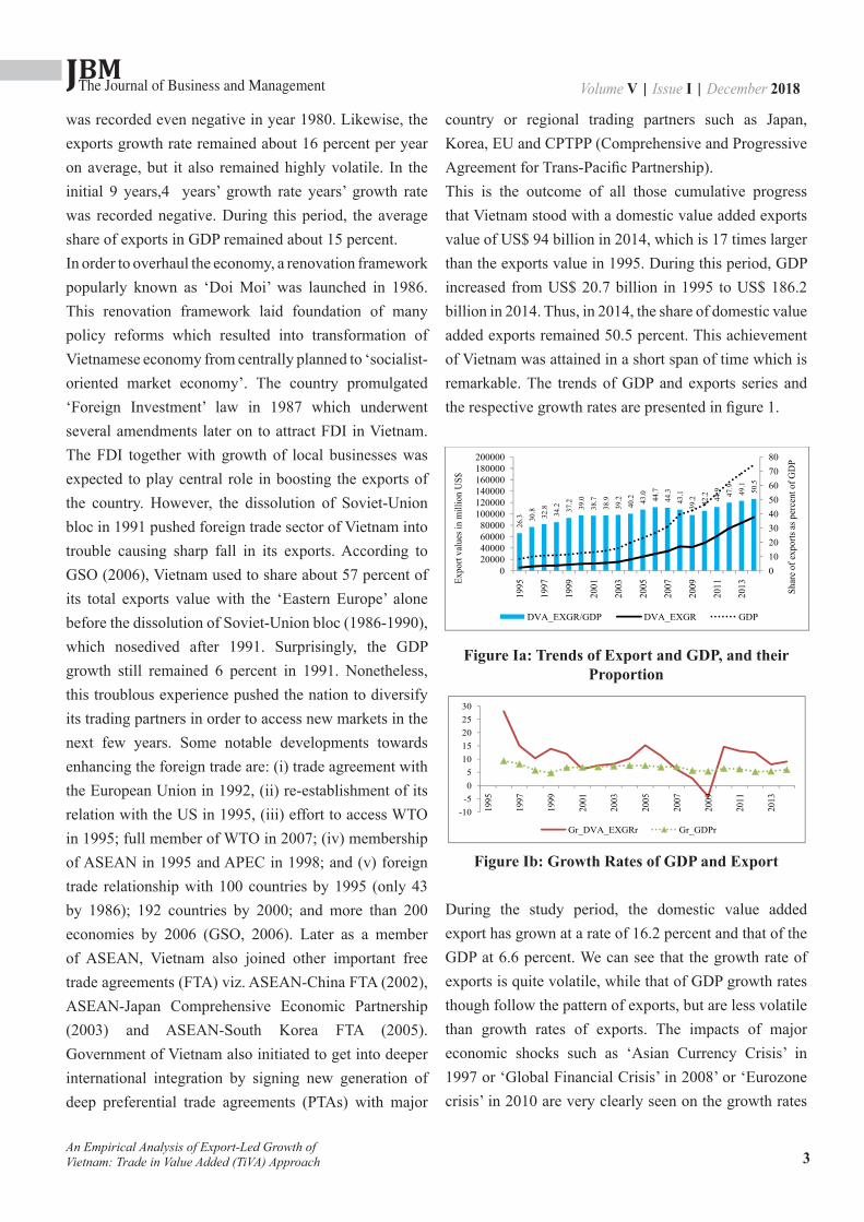
country or regional trading partners such as Japan, Korea, EU and CPTPP (Comprehensive and Progressive Agreement for Trans-Pacific Partnership).This is the outcome of all those cumulative progress that Vietnam stood with a domestic value added exports value of US$ 94 billion in 2014, which is 17 times larger than the exports value in 1995. During this period, GDP increased from US$ 20.7 billion in 1995 to US$ 186.2 billion in 2014. Thus, in 2014, the share of domestic value added exports remained 50.5 percent. This achievement of Vietnam was attained in a short span of time which is remarkable. The trends of GDP and exports series and the respective growth rates are presented in figure 1.
(5)
Nonetheless, this troublous experience pushed the nation to diversify its trading partners in
order to access new markets in the next few years. Some notable developments towards
enhancing the foreign trade are: (i) trade agreement with the European Union in 1992, (ii)
re-establishment of its relation with the US in 1995, (iii) effort to access WTO in 1995;
full member of WTO in 2007; (iv) membership of ASEAN in 1995 and APEC in 1998;
and (v) foreign trade relationship with 100 countries by 1995 (only 43 by 1986); 192
countries by 2000; and more than 200 economies by 2006 (GSO, 2006). Later as a
member of ASEAN, Vietnam also joined other important free trade agreements (FTA) viz.
ASEAN-China FTA (2002), ASEAN-Japan Comprehensive Economic Partnership (2003)
and ASEAN-South Korea FTA (2005). Government of Vietnam also initiated to get into
deeper international integration by signing new generation of deep preferential trade
agreements (PTAs) with major country or regional trading partners such as Japan, Korea,
EU and CPTPP (Comprehensive and Progressive Agreement for Trans-Pacific
Partnership).
This is the outcome of all those cumulative progress that Vietnam stood with a domestic
value added exports value of US$ 94 billion in 2014, which is 17 times larger than the
exports value in 1995. During this period, GDP increased from US$ 20.7 billion in 1995 to
US$ 186.2 billion in 2014. Thus, in 2014, the share of domestic value added exports
remained 50.5 percent. This achievement of Vietnam was attained in a short span of time
which is remarkable. The trends of GDP and exports series and the respective growth rates
are presented in figure 1.
Figure 1a: Trends of export and GDP, and their proportion
26.3 30
.8 32.8
34.2 37
.2 39.0
38.7
38.9
39.2
40.2 43
.044
.744
.343
.139
.2 42.2 44
.9 47.9
49.1
50.5
01020304050607080
020000400006000080000
100000120000140000160000180000200000
1995
1997
1999
2001
2003
2005
2007
2009
2011
2013 Sh
are
of e
xpor
ts as
per
cent
of G
DP
Expo
rt va
lues
in m
illio
n U
S$
DVA_EXGR/GDP DVA_EXGR GDP
Figure Ia: Trends of Export and GDP, and their Proportion
(6)
Figure 1b: Growth rates of GDP and Export
During the study period, the domestic value added export has grown at a rate of 16.2
percent and that of the GDP at 6.6 percent. We can see that the growth rate of exports is
quite volatile, while that of GDP growth rates though follow the pattern of exports, but are
less volatile than growth rates of exports. The impacts of major economic shocks such as
‘Asian Currency Crisis’ in 1997 or ‘Global Financial Crisis’ in 2008’ or ‘Eurozone crisis’
in 2010 are very clearly seen on the growth rates of exports. Moreover, the impact of
financial crisis is severe. Aftermath crisis, the exports growth rates are negative and the
GDP growth rate also fell substantially (7.1 percent in 2007 to 5.7 percent in 2008 and 5.4
percent in 2009). However, by 2010, Vietnam has made a breakthrough in terms of
exports and GDP growths and clear signs of recovery can be observed. But again after
2010 until 2014, growths of exports are falling. Thus, though growth rate of GDP has
shown weak sensitivity to the shocks in export growth rate, there is quite higher
correlation (correlation coefficient above 0.99) in terms of dollar values.
III. Methodological framework
The contribution of exports to the economic growth of Vietnam has been analysed through
examination of existence of a long-run relationship between the domestic value added
exports (DVA_EXGR) and gross domestic products (GDP), both measured in real terms.
Empirically, the long-run relationship between two variables in question can be tested by
-10-505
1015202530
1995
1997
1999
2001
2003
2005
2007
2009
2011
2013
Gr_DVA_EXGRr Gr_GDPr
Figure Ib: Growth Rates of GDP and Export
During the study period, the domestic value added export has grown at a rate of 16.2 percent and that of the GDP at 6.6 percent. We can see that the growth rate of exports is quite volatile, while that of GDP growth rates though follow the pattern of exports, but are less volatile than growth rates of exports. The impacts of major economic shocks such as ‘Asian Currency Crisis’ in 1997 or ‘Global Financial Crisis’ in 2008’ or ‘Eurozone crisis’ in 2010 are very clearly seen on the growth rates
An Empirical Analysis of Export-Led Growth of Vietnam: Trade in Value Added (TiVA) Approach

JBMVolume V | Issue I | December 2018The Journal of Business and Management
4
of exports. Moreover, the impact of financial crisis is severe. Aftermath crisis, the exports growth rates are negative and the GDP growth rate also fell substantially (7.1 percent in 2007 to 5.7 percent in 2008 and 5.4 percent in 2009). However, by 2010, Vietnam has made a breakthrough in terms of exports and GDP growths and clear signs of recovery can be observed. But again after 2010 until 2014, growths of exports are falling. Thus, though growth rate of GDP has shown weak sensitivity to the shocks in export growth rate, there is quite higher correlation (correlation coefficient above 0.99) in terms of dollar values.
3. Data and MethodologyThe contribution of exports to the economic growth of Vietnam has been analysed through examination of existence of a long-run relationship between the domestic value added exports (DVA_EXGR) and gross domestic products (GDP), both measured in real terms. Empirically, the long-run relationship between two variables in question can be tested by using either (i) two-step Engle and Granger approach, or (ii) cointegration approach, or (iii) ARDL (autoregressive distributed lags) approach. However, the first two approaches require the underlying variables to be integrated of same order one, I(1), while the ARDL approach does not require the underlying variables to be integrated of the same order one, though none of them should be integrated of the order higher than one. This means that it is essential to test the presence of unit root and also to determine the order of integration for each of these variables if someone opts to apply the Engle and Granger approach, or cointegration approach. On the other hand, ARDL approach is applicable despite the underlying variables show a mixed order of integration, i.e. I(0) and I(1). This flexible feature of ARDL approach has made it popular in recent days as a technique to test existence of a long-run relationship.Whilst the ARDL approach does not require testing the order of integration of variables beforehand, we have preferred to do it beforehand for two reasons- (i) at this moment,we don’t know which approach would best fit to
model the existence of cointegration between underlying variables. Therefore, it is better to know their order of integration beforehand, (ii) though ARDL approach seems flexible in the initial steps in ignoring the order of integration of variables, it requires at later steps to confirm that none of these variables are integrated of order 2.At current level of literature, there are two approaches to examine the presence of unit roots in variables’ series viz. (i) the unit root test that does not allow structural break (hence after we will call it ‘CURT’- the conventional unit root test); and (ii) the unit root test that allows structural break (hence after we call it ‘BURT’- the breakpoint unit root test). The CURT can be conducted using Augmented Dickey-Fuller (ADF), Phillips-Perron (PP), Kwiatkowski, Phillips, Schmidt, and Shin (KPSS), Ng-Perron test etc. However, Perron (1989) by re-examining Nelson and Plosser’s work (1982) by incorporating two important structural breaks, that is, ‘the great crash of 1929’ and ‘the oil price shock of 1973’ in the underlying variables series, found that CURT test might falsely result into presence of unit root when the data are ‘trend stationary’ with structural break(s). Surprisingly, 10 out of 13 nonstationary series were found stationary in their level forms when structural breaks were introduced in the test. Thereby Perron (1989) cautions that although use of long-span data in testing presence of a unit root allows tests with larger power in comparison to using a smaller span; however; drawback is that the long-span data may include effect of a major event, which may behave as an outlier. In the light of Perron’s caution, a researcher must be aware of the presence of outlier(s) while considering a long-span data series for testing a unit root; otherwise the use of CURT to validate the stationarity of time series might be misleading if a structural break is present in it. In this research, the underlying variables (i.e. GDP and domestic value added exports) cover a period from 1995 to 2014 for which the existing sets of literature strongly suggest possibility of structural break(s). There are at least three reasons behind this suspicion- (i) occurrence of ‘Asian financial crisis’ affecting ASEAN region in
An Empirical Analysis of Export-Led Growth of Vietnam: Trade in Value Added (TiVA) Approach

JBMVolume V | Issue I | December 2018The Journal of Business and Management
5
1997, (ii) occurrence of ‘Global financial crisis’ in 2008 affecting the US and Euro zone, which are major markets for Vietnamese exports, and (iii) Ling et al. (2013) found presence of structural breaks in 10 macroeconomic time-series, including GDP and exports of ASEAN countries during the period of 1960-2010. They found that common structural break occurred among these ASEAN macroeconomic time series were closely associated with global economic events such as the first oil shock of 1973-1975, the second oil shock of 1979-1980, the commodity crisis in 1985-1986 and the Asian financial crisis of 1997-1998. As Vietnam is also located in and connected with the ASEAN region, such possibility cannot be denied.However, there are some empirical works in context of Vietnam viz. Nguyen et al. (2017), Nguyen (2017), Duong (2016), Bhatt (2013), and Pham (2008) who have applied CURT approach on GDP and exports series of Vietnam to test presence of unit roots, thus overlooking the possibility of presence of structural break in GDP and exports series. All of these papers though agree that order of integration of exports series is one, I(1) in level form, they differ in determining order of integration of GDP series. Nguyen et al. (2017) and Bhat (2013) concludes it as I(1), while Nguyen (2017) confirms it to be I(0) (table 1).Upon thoughtful consideration on the facts and scenarios as discussed above, we realised that it would be better to use BURT approach to confirm the stationarity and the order of integration of the underlying variables series.
Table I: Empirical Papers Using Data Series on Exports and GDP of Vietnam
Reference Variable Cover-age
Order of integration
Meth-od
Nguyen et al. (2017)
Net exports and GDP
1990-2015 Both I(1) CURT
Nguyen (2017) Exports and
GDP1986-2015
Export (1);
GDP I(0)CURT
Duong (2016) Exports 1985-
2015 I(1) CURTBhatt (2013)
Exports and GDP
1990-2008 BothI(1) CURT
Pham (2008) Exports 1986-
2007 I(1) CURT
3.1 Unit Root Test in Presence of a Single Structural Break
Perron’s work (1989) is a prominent initiative to introduce structural break in the unit root test framework. He considered three different models to test null hypothesis of a unit root against the alternative hypothesis of deterministic trend with a one-time exogeneous break in - (A) the level of the series (aka ‘crash model’), (B) the slope (aka ‘changing growth model’); and (C) both the level and slope. These hypotheses are parameterized as follows:Null hypotheses:Model (A): yt = µ + dD(TB)t + yt-1 + et
Model (B): yt = µ1 + yt-1 + (µ2 - µ1)DUt + et
Model (C): yt = µ1 + yt-1 + dD(TB)t + (µ2 - µ1)DUt + et
Here DUt is ‘intercept break’ variable that takes the value of 0 for all dates prior to the break, and 1 thereafter (i.e. DUt = 1, if t > TB, 0 otherwise). Likewise, D(TB)t is ‘one-time break dummy’ variable which takes the value of 1 only on the break date and 0 otherwise, (i.e. D(TB)t = 1, if t = TB + 1, 0 otherwise).Alternative hypotheses:Model (A): yt = µ1 + βt + (µ2 - µ1)DUt + et
Model (B): yt = µ + β1t + (β2 - β1)DT*t + et
Model (C): yt = µ1 + β1t + (µ2 - µ1)DUt + (β2 - β1)DTt + et
Here DT*t is ‘trend break’ variable which takes the value
0 for all dates prior to the break, and is a break date re-based trend for all subsequent dates (i.e.DT*
t = t – TB if t > TB and 0 otherwise).In these models, the difference (µ2 - µ1) represents the magnitude of the change in the intercept of the trend function at time TB, and the difference (β2 - β1) represents the magnitude of the change in the slope of the trend function occurring at time TB. The innovation series {et} is taken to be of the ARMA(p, q), the orders p and q possibly unknown.The null hypothesis of a unit root in the model (A) is presented in term of a dummy variable, which takes the value one at the time of break, while the alternative hypothesis allows for a one-time change in the intercept of the trend function. Likewise, the null hypothesis of the model (B) specifies that the drift parameter µ changes
An Empirical Analysis of Export-Led Growth of Vietnam: Trade in Value Added (TiVA) Approach
JBMVolume V | Issue I | December 2018The Journal of Business and Management
6
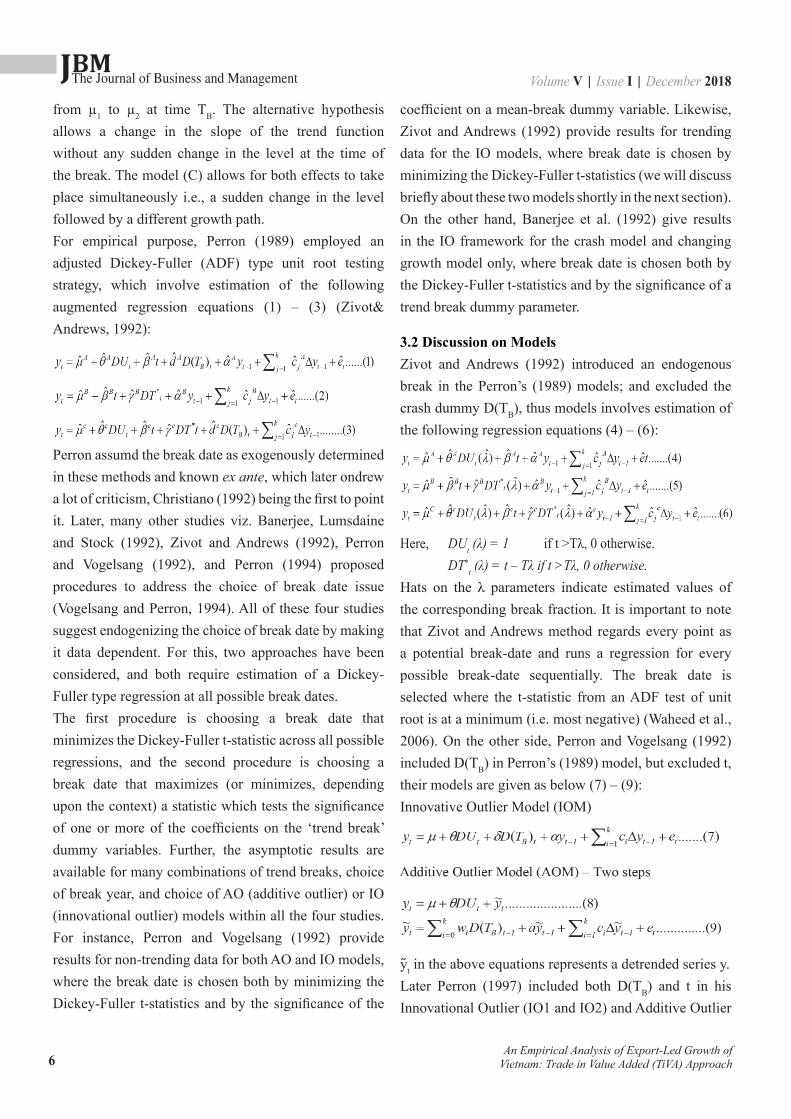
from µ1 to µ2 at time TB. The alternative hypothesis allows a change in the slope of the trend function without any sudden change in the level at the time of the break. The model (C) allows for both effects to take place simultaneously i.e., a sudden change in the level followed by a different growth path.For empirical purpose, Perron (1989) employed an adjusted Dickey-Fuller (ADF) type unit root testing strategy, which involve estimation of the following augmented regression equations (1) – (3) (Zivot& Andrews, 1992):
Perron assumd the break date as exogenously determined in these methods and known ex ante, which later ondrew a lot of criticism, Christiano (1992) being the first to point it. Later, many other studies viz. Banerjee, Lumsdaine and Stock (1992), Zivot and Andrews (1992), Perron and Vogelsang (1992), and Perron (1994) proposed procedures to address the choice of break date issue (Vogelsang and Perron, 1994). All of these four studies suggest endogenizing the choice of break date by making it data dependent. For this, two approaches have been considered, and both require estimation of a Dickey-Fuller type regression at all possible break dates.The first procedure is choosing a break date that minimizes the Dickey-Fuller t-statistic across all possible regressions, and the second procedure is choosing a break date that maximizes (or minimizes, depending upon the context) a statistic which tests the significance of one or more of the coefficients on the ‘trend break’ dummy variables. Further, the asymptotic results are available for many combinations of trend breaks, choice of break year, and choice of AO (additive outlier) or IO (innovational outlier) models within all the four studies. For instance, Perron and Vogelsang (1992) provide results for non-trending data for both AO and IO models, where the break date is chosen both by minimizing the Dickey-Fuller t-statistics and by the significance of the
coefficient on a mean-break dummy variable. Likewise, Zivot and Andrews (1992) provide results for trending data for the IO models, where break date is chosen by minimizing the Dickey-Fuller t-statistics (we will discuss briefly about these two models shortly in the next section). On the other hand, Banerjee et al. (1992) give results in the IO framework for the crash model and changing growth model only, where break date is chosen both by the Dickey-Fuller t-statistics and by the significance of a trend break dummy parameter.
3.2 Discussion on ModelsZivot and Andrews (1992) introduced an endogenous break in the Perron’s (1989) models; and excluded the crash dummy D(TB), thus models involves estimation of the following regression equations (4) – (6):
Here, DUt (λ) = 1 if t >Tλ, 0 otherwise. DT*
t (λ) = t – Tλ if t >Tλ, 0 otherwise.Hats on the λ parameters indicate estimated values of the corresponding break fraction. It is important to note that Zivot and Andrews method regards every point as a potential break-date and runs a regression for every possible break-date sequentially. The break date is selected where the t-statistic from an ADF test of unit root is at a minimum (i.e. most negative) (Waheed et al., 2006). On the other side, Perron and Vogelsang (1992) included D(TB) in Perron’s (1989) model, but excluded t, their models are given as below (7) – (9):Innovative Outlier Model (IOM)
yt in the above equations represents a detrended series y.Later Perron (1997) included both D(TB) and t in his Innovational Outlier (IO1 and IO2) and Additive Outlier
An Empirical Analysis of Export-Led Growth of Vietnam: Trade in Value Added (TiVA) Approach

JBMVolume V | Issue I | December 2018The Journal of Business and Management
7
(AO) models, which are presented as below (10) – (12): IO model allowing one time change in intercept only (IO1):
IO model allowing one time change in both intercept and slope (IO2)
AO model allowing one time change in slope (AO)
Among bunch of these models, like any other researcher, we also faced the problem of selecting an appropriate
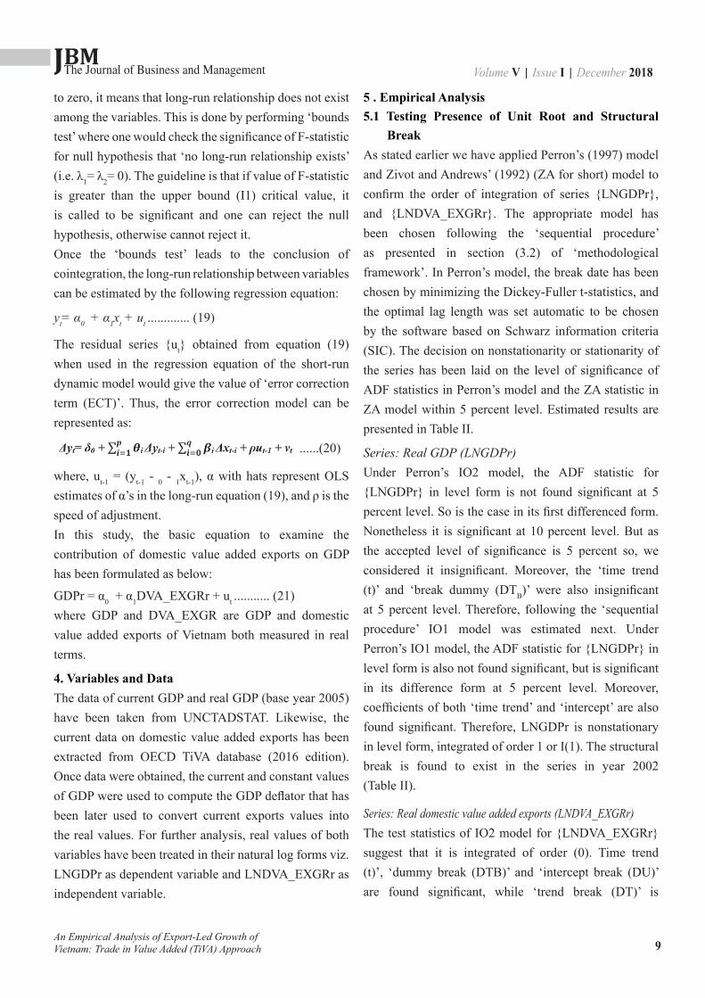
model to determine the stationarity of a time series in presence of structural break. Results of different models in different test specification viz. (i) with intercept only, (ii) with trend only or (iii) with both intercept and trend were likely to differ, causing confusion in terms of inclusion of irrelevant information and the exclusion of relevant information. In either case, the model might be misleading. Nonetheless, in order to overcome this state of confusion Shrestha and Chowdhury’s paper (2005) on ‘sequential procedure’ becomes an effective guideline, and thereby we have followed their sequential procedure in the unit root analysis. A flow-chart based on this paper has been presented in figure 2. Other aspects of these models have been discussed in the ‘empirical results’ section.
An Empirical Analysis of Export-Led Growth of Vietnam: Trade in Value Added (TiVA) Approach
(14)
Figure 2: Flow chart for the sequential procedure
Source: Researchers’ contribution based on sequential procedure described in Shrestha and Chowdhury’s paper (2005).
t = time trend DTB= one-time break dummy DU= intercept break DT= trend break PV= Perron and Vogelsang
Run Perron (1997) IO2 Model
t
Is t significant?
Yes
Is DTB significant?
Yes No No
Check DU & DT
DTB
Check these
Is DU significant? Is DT significant?
Yes No Yes No
Select the model
Run Perrron (1997) IO1 Model
Run Perron (1997) AO model
Run ZA (1992) model
Run PV (1992) model
Check IO1/AO Model
Figure II: Flow Chart for the Sequential ProcedureSource: Researchers’ contribution based on sequential procedure described in Shrestha and Chowdhury’s paper (2005).

JBMVolume V | Issue I | December 2018The Journal of Business and Management
8
3.3 Cointegration Test3.3.1 Engel-Granger ApproachThe first step of Engle-Granger approach requires testing for unit roots in variable series, after which two cointegration regressions (direct and reverse) between variables are estimated using ordinary least square (OLS)1 method. The second step involves testing stationarity in the error terms of the two cointegration regressions as estimated in the first step. According to Engle and Granger (1987), if the stochastic error terms are integrated of order zero, I(0), then yt and xt are said to be cointegrated. In this case, residuals from the equilibrium regression can be used to estimate the error correction model.Hence, if variables series {yt} and {xt} are cointegrated, the variables would have the error correction form as below:
where ∆ is first difference operator on variables, εxtand εytare white noise disturbances (which may be correlated with each other), and α’s and β’s are all parameters. The ρt-1 is the error correction term (ECT) whose magnitude (αx or βy) is expected to be a negative fraction between 0 and unity, and implies a ‘speed of adjustment’ per year of any deviation from the long run equilibrium path in order to maintain the long-run equilibrium relation between underlying variables. The independent variables are said to ‘cause’ the dependent variable if the error correction term (ECT), and the coefficients of the lagged independent variables (summation of α2iin equation (13) and summation of β1iin equation (14)) are jointly significant.
3.3.2 Johansen TestJohansen (1988) test of cointegration is based on the relationship between the rank of matrix and its
characteristics roots. Its generalised model can be written in form of a vector auto regression (VAR) in levels with the constant suppressed as:
13) ∆xt = α0 + αx ρt-1 + ∑=
−p
1i1ti1 xΔα + ∑
=−
p
1i1ti2 yΔα + εxt
(14) ∆yt = β0 + βy ρt-1 + ∑=
−p
1i1ti1 xΔβ + ∑
=−
p
1i1ti2 yΔβ + εyt
xt= ∑=
−k
1iiti xA + ut
Δyt= δ0 + 𝜽𝜽𝒑𝒑𝒊𝒊$𝟏𝟏 i Δyt-i + 𝜷𝜷𝒒𝒒
𝒊𝒊$𝟎𝟎 i Δxt-i + δ1t + λ1yt-1 + λ2xt-1 + et
Δyt= δ0 + 𝜽𝜽𝒑𝒑𝒊𝒊$𝟏𝟏 i Δyt-i + 𝜷𝜷𝒒𝒒
𝒊𝒊$𝟎𝟎 i Δxt-i + ρut-1 + vt
............. (15)
For the simpler case k = 1, it is simply-
Δxt= (A1-I) xt-1+et = Π xt-1+et............. (16)
where, xt and et are (n×1) vectors; A1= an (n×n) matrix of parameters; I = an (n×n) identity matrix; and Π = A1-I, n is the number of variables.The Johansen test examines the rank of Π matrix. If the rank (Π) = 0, then the variables are not cointegrated, otherwise they are said to be cointegrated. In fact the rank of Π provides the number of cointegrating vectors. Further, the Johansen test comprises of two tests: the maximum eigenvalue test, and the trace test. For both test statistics, the initial Johansen test is a test of the null hypothesis of no cointegration against the alternative of cointegration. These tests differ in terms of the alternative hypothesis.
3.3.3 ARDL Bounds TestThe basic form of an ARDL (p, q) regression model can be represented as follow:yt= δ0 + δ1t + θ1yt-1 + θ2yt-2 + … + θpyt-p + β1xt-1 + β2xt-2 + … + βqxt-q + et ...............(17)
Pesaran et al. (2001) reduced the basic form of ARDL to the conditional error correction form in their seminal paper which got the most attention in applied work to test for the existence of long-run relationship. Their conditional error correction form of ARDL model can be represented as follow:
where Δ represents the first difference operator; θ’s are the short-run coefficients and all the terms in the summations are the short-run dynamics of the model; λ’s are the long-run coefficients, and e is the error term of the equation.For testing the long-run relationship, the interest is to test that λ1 and λ2 are non-zero. If these are statistically equal
An Empirical Analysis of Export-Led Growth of Vietnam: Trade in Value Added (TiVA) Approach
JBMVolume V | Issue I | December 2018The Journal of Business and Management
9
to zero, it means that long-run relationship does not exist among the variables. This is done by performing ‘bounds test’ where one would check the significance of F-statistic for null hypothesis that ‘no long-run relationship exists’ (i.e. λ1= λ2= 0). The guideline is that if value of F-statistic is greater than the upper bound (I1) critical value, it is called to be significant and one can reject the null hypothesis, otherwise cannot reject it. Once the ‘bounds test’ leads to the conclusion of cointegration, the long-run relationship between variables can be estimated by the following regression equation:
yt= α0 + α1xt + ut ............. (19)
The residual series {ut} obtained from equation (19) when used in the regression equation of the short-run dynamic model would give the value of ‘error correction term (ECT)’. Thus, the error correction model can be represented as:
......(20)
where, ut-1 = (yt-1 - 0 - 1xt-1), α with hats represent OLS estimates of α’s in the long-run equation (19), and ρ is the speed of adjustment.In this study, the basic equation to examine the contribution of domestic value added exports on GDP has been formulated as below:
GDPr = α0 + α1DVA_EXGRr + ut ........... (21)where GDP and DVA_EXGR are GDP and domestic value added exports of Vietnam both measured in real terms.
4. Variables and DataThe data of current GDP and real GDP (base year 2005) have been taken from UNCTADSTAT. Likewise, the current data on domestic value added exports has been extracted from OECD TiVA database (2016 edition). Once data were obtained, the current and constant values of GDP were used to compute the GDP deflator that has been later used to convert current exports values into the real values. For further analysis, real values of both variables have been treated in their natural log forms viz. LNGDPr as dependent variable and LNDVA_EXGRr as independent variable.
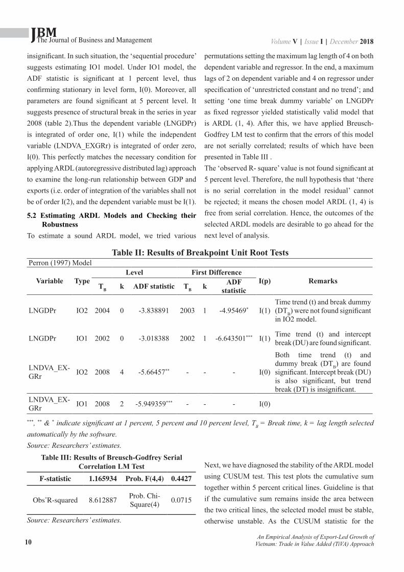
5 . Empirical Analysis5.1 Testing Presence of Unit Root and Structural
BreakAs stated earlier we have applied Perron’s (1997) model and Zivot and Andrews’ (1992) (ZA for short) model to confirm the order of integration of series {LNGDPr}, and {LNDVA_EXGRr}. The appropriate model has been chosen following the ‘sequential procedure’ as presented in section (3.2) of ‘methodological framework’. In Perron’s model, the break date has been chosen by minimizing the Dickey-Fuller t-statistics, and the optimal lag length was set automatic to be chosen by the software based on Schwarz information criteria (SIC). The decision on nonstationarity or stationarity of the series has been laid on the level of significance of ADF statistics in Perron’s model and the ZA statistic in ZA model within 5 percent level. Estimated results are presented in Table II.
Series: Real GDP (LNGDPr)Under Perron’s IO2 model, the ADF statistic for {LNGDPr} in level form is not found significant at 5 percent level. So is the case in its first differenced form. Nonetheless it is significant at 10 percent level. But as the accepted level of significance is 5 percent so, we considered it insignificant. Moreover, the ‘time trend (t)’ and ‘break dummy (DTB)’ were also insignificant at 5 percent level. Therefore, following the ‘sequential procedure’ IO1 model was estimated next. Under Perron’s IO1 model, the ADF statistic for {LNGDPr} in level form is also not found significant, but is significant in its difference form at 5 percent level. Moreover, coefficients of both ‘time trend’ and ‘intercept’ are also found significant. Therefore, LNGDPr is nonstationary in level form, integrated of order 1 or I(1). The structural break is found to exist in the series in year 2002 (Table II).
Series: Real domestic value added exports (LNDVA_EXGRr)The test statistics of IO2 model for {LNDVA_EXGRr} suggest that it is integrated of order (0). Time trend (t)’, ‘dummy break (DTB)’ and ‘intercept break (DU)’ are found significant, while ‘trend break (DT)’ is
An Empirical Analysis of Export-Led Growth of Vietnam: Trade in Value Added (TiVA) Approach
JBMVolume V | Issue I | December 2018The Journal of Business and Management
10
insignificant. In such situation, the ‘sequential procedure’ suggests estimating IO1 model. Under IO1 model, the ADF statistic is significant at 1 percent level, thus confirming stationary in level form, I(0). Moreover, all parameters are found significant at 5 percent level. It suggests presence of structural break in the series in year 2008 (table 2).Thus the dependent variable (LNGDPr) is integrated of order one, I(1) while the independent variable (LNDVA_EXGRr) is integrated of order zero, I(0). This perfectly matches the necessary condition for applying ARDL (autoregressive distributed lag) approach to examine the long-run relationship between GDP and exports (i.e. order of integration of the variables shall not be of order I(2), and the dependent variable must be I(1).
5.2 Estimating ARDL Models and Checking their Robustness
To estimate a sound ARDL model, we tried various
permutations setting the maximum lag length of 4 on both dependent variable and regressor. In the end, a maximum lags of 2 on dependent variable and 4 on regressor under specification of ‘unrestricted constant and no trend’; and setting ‘one time break dummy variable’ on LNGDPr as fixed regressor yielded statistically valid model that is ARDL (1, 4). After this, we have applied Breusch-Godfrey LM test to confirm that the errors of this model are not serially correlated; results of which have been presented in Table III . The ‘observed R- square’ value is not found significant at 5 percent level. Therefore, the null hypothesis that ‘there is no serial correlation in the model residual’ cannot be rejected; it means the chosen model ARDL (1, 4) is free from serial correlation. Hence, the outcomes of the selected ARDL models are desirable to go ahead for the next level of analysis.
Table II: Results of Breakpoint Unit Root TestsPerron (1997) Model
Variable TypeLevel First Difference
I(p) RemarksTB k ADF statistic TB k ADF
statistic
LNGDPr IO2 2004 0 -3.838891 2003 1 -4.95469* I(1)Time trend (t) and break dummy (DTB) were not found significant in IO2 model.
LNGDPr IO1 2002 0 -3.018388 2002 1 -6.643501*** I(1) Time trend (t) and intercept break (DU) are found significant.
LNDVA_EX-GRr IO2 2008 4 -5.66457** - - - I(0)
Both time trend (t) and dummy break (DTB) are found significant. Intercept break (DU) is also significant, but trend break (DT) is insignificant.
LNDVA_EX-GRr IO1 2008 2 -5.949359*** - - - I(0)
***, ** & * indicate significant at 1 percent, 5 percent and 10 percent level, TB = Break time, k = lag length selected automatically by the software. Source: Researchers’ estimates.
An Empirical Analysis of Export-Led Growth of Vietnam: Trade in Value Added (TiVA) Approach
Table III: Results of Breusch-Godfrey Serial Correlation LM Test
F-statistic 1.165934 Prob. F(4,4) 0.4427
Obs*R-squared 8.612887Prob. Chi-Square(4)
0.0715
Source: Researchers’ estimates.
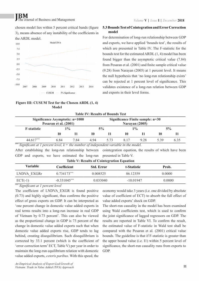
Next, we have diagnosed the stability of the ARDL model using CUSUM test. This test plots the cumulative sum together within 5 percent critical lines. Guideline is that if the cumulative sum remains inside the area between the two critical lines, the selected model must be stable, otherwise unstable. As the CUSUM statistic for the
JBMVolume V | Issue I | December 2018The Journal of Business and Management
11
chosen model lies within 5 percent critical bands (figure 3), means absence of any instability of the coefficients in the ARDL model.
-10.0
-7.5
-5.0
-2.5
0.0
2.5
5.0
7.5
10.0
2007 2008 2009 2010 2011 2012 2013 2014
CUSUM 5% Significance
Model DVA
Figure III: CUSUM Test for the Chosen ARDL (1, 4) Model
5.3 Bounds Test of Cointegration and Error Correction model
For determination of long-run relationship between GDP and exports, we have applied ‘bounds test’, the results of which are presented in Table IV. The F-statistic for the bounds test for the estimated ARDL (1, 4) model has been found bigger than the asymptotic critical value (7.84) from Pesaran et al. (2001) and finite sample critical value (9.28) from Narayan (2005) at 1 percent level. It means the null hypothesis that ‘no long-run relationship exists’ can be rejected at 1 percent level of significance. This validates existence of a long-run relation between GDP and exports in their level forms.
An Empirical Analysis of Export-Led Growth of Vietnam: Trade in Value Added (TiVA) Approach
Table IV: Results of Bounds TestSignificance Asymptotic: n=1000
Pesaran et al. (2001)Significance Finite sample: n=30
Narayan (2005)F-statistic 1% 5% 1% 5%
I0 I1 I0 I1 I0 I1 I0 I1
44.617*** 6.84 7.84 4.94 5.73 8.17 9.28 5.39 6.35*** Significant at 1 percent level, k = the number of independent variable in the model.
The coefficient of LNDVA_EXGR is found positive (0.73) and highly significant, thus confirms the positive effect of gross exports on GDP. It can be interpreted as ‘one percent change in domestic value added exports in real terms results into a long-run increase in real GDP of Vietnam by 0.73 percent’. This can also be viewed as the proportional change in GDP is 73 percent of the change in domestic value added exports such that when domestic value added exports rise, GDP tends to lag behind, creating disequilibrium. Such disequilibrium is corrected by 33.1 percent (which is the coefficient of ‘error correction term’ ECT, Table V) per year in order to maintain the long-run equilibrium relation with domestic value added exports, ceteris paribus. With this speed, the
economy would take 3 years (i.e. one divided by absolute value of coefficient of ECT) to absorb the full effect of value added exports’ shock on GDP.The short-run causality in the model has been examined using Wald coefficients test, which is used to confirm the joint significance of lagged regressors on GDP. The results are reported in Table VI. To confirm the result, the estimated value of F-statistic in Wald test shall be compared with the Pesaran et al. (2001) critical value bounds. The guideline is that if F-statistic is greater than the upper bound value (i.e. I1) within 5 percent level of significance, the short-run causality runs from exports to GDP.
After establishing the long-run relationship between GDP and exports, we have estimated the long-run
cointegration equation, the results of which have been presented in Table V.
Table V: Results of Cointegration EquationVariable Coefficient Std. Error t-Statistic Prob.
LNDVA_EXGRr 0.734173*** 0.008525 86.12359 0.0000
ECT(-1) -0.331045*** 0.033040 -10.01947 0.0000*** Significant at 1 percent level

JBMVolume V | Issue I | December 2018The Journal of Business and Management
12An Empirical Analysis of Export-Led Growth of
Vietnam: Trade in Value Added (TiVA) Approach
Table VI: Results of Wald TestAsymptotic critical value bounds for the F-statistic#, k=1
(Case III: Unrestricted intercept and no trend)Test Statistic Value df 1% Significance 5% SignificanceF-statistic 17.895*** (5, 8) I0 I1 I0 I1Chi-square 89.473 5 11.79 11.79 4.94 5.73
*** & ** Significant at 1 percent and 5 percent level respectively. # Pesaran et al. (2001, p.300), k= number of regressor.
Interestingly, the estimated F statistic is greater than the upper values at 5 percent level of significance, thus qualify the guideline. Hence, it can be concluded that causality exists between exports and GDP in the short-run i.e. ‘exports short-run causes GDP’.
6. ConclusionVietnam prioritized export expansion since its adoption of ‘Doi Moi’ in 1986, following the footstep of Japan, Singapore, Hong Kong, Taiwan, and South Korea. To enhance its access to foreign markets and promote exports, Vietnam also did some notable developments in the 1990s in signing bilateral and multilateral trade agreements. Visibly, since 1995 Vietnam has consistently achieved higher economic growth relying on exports, and been reaping the benefit of export-based strategy in terms of job creation, foreign reserves, and improving living standard. The ARDL bounds test of cointegration establishes existence of both short-run and long-run relationship between exports and GDP of Vietnam and shows a substantial contribution of exports in the real GDP, as much as 0.73 percent for one percent changes in the domestic value added exports. This is a fascinating number. However, a huge question is whether Vietnam can sustain this growth. To answer this question, we shall look at the growth prospective of Vietnam from two perspectives:
i. Inherent bottleneck in the export-led growth model: The overall exports pattern of Vietnam portrays it following the footsteps of export-led growth model of Mexico, whereby it has also turned itself into export production platforms for foreign multi-nationals by suppressing the wages, rather than developing own indigenous industrial capacity. Mexico model of export-led growth strategy is different from the
one adopted by Germany or Japan or Asian Four Tiger countries or China. These countries’ export strategies led to enhance their own industrial capacity. Nonetheless, the Mexico model has been less successful so far. Mexico has not yet recovered its strong performance of 1960–1980. Since 1980, GDP growth has been sluggish, labor productivity has been unchanged, and total factor productivity growth has been negative.Considering the prerequisites for the Mexico model to work, it seems challenging for Vietnam to sustain its export-led growth which it has achieved so far. With the rising living standards, ultimately the comparative advantages of cheap labour force would vanish in the future, which means a wave of assembly jobs would flow out of Vietnam leaving masses of workers without jobs, creating dark days in the country. In addition, two other low-cost countries in the region, Cambodia and Myanmar are likely to rise as close competitors of Vietnam in the low cost assembly works in the near future. By that time, in case Vietnam fails to enter into higher value added tasks due to lack of adequate skills or technologies or both, it will drag itself into ‘middle income trap’ (a situation when a country cannot compete in low value added stages due to rising labour costs, and also cannot compete in higher value added stages due to lack of adequate skills and technologies).
ii. Changing political and macroeconomic situations: Another challenge in the existing model is to manage risks that would originate from ‘supply shocks’ and ‘demand shocks’. Though Government of Vietnam has initiated to get into deeper international integration by signing new generation of deep
JBMVolume V | Issue I | December 2018The Journal of Business and Management
13
preferential trade agreements (PTAs) with major trading partners such as Japan, Korea, EU and CPTPP apart from ASEAN-China FTA (2002), ASEAN-Japan Comprehensive Economic Partnership (2003), and ASEAN-South Korea FTA (2005, the changing macroeconomic situations that has developed across major trading partners of Vietnam in past few years has led to believe that the export-led growth strategy will fray for Vietnam. For instance, US consumers are debt saturated, and the US government is now more concerned about imports from outside. Europe is constrained by fiscal austerity. Japan continues to suffer from weak internal demand, and is also still hooked on export-oriented growth. That means if these macroeconomic conditions sustain the foreign demand for Vietnam’s exports would weaken for sure that might have catastrophic impact on its economic growth.
Therefore, the ‘assembling platform’ strategy shall be bonded with strategy to develop own indigenous industrial capacity, and national technological base. These will help Vietnam to upgrade its activities along value chains in forms of (i) product upgrading, (ii)
process upgrading, (iii) functional upgrading, and/or (iv) sectoral upgrading so that it can switch its role of ‘assembling agent’ to ‘indigenous producer’. Of course, these do not seem feasible in a short term since a large proportion of Vietnamese labour forces lack adequate skills and expertise that are necessary to carry out such activities. In addition, Vietnam also lacks ‘Vietnamese brand name’ in international market at present time that has made it relying on foreign companies for marketing abroad. Therefore, in the meantime, government shall also prioritize involvement of domestic firms in global value chains. All of these require prompt initiatives in order to bring changes in the existing ‘education and vocational training’ related policies so that knowledge, skills and know-how of young generations can be enhanced. Likewise, Vietnam shall enter into more deep preferential trade agreements (PTAs) with its trading partners to be able to manage the supply and demand shocks to exports. In addition, it shall also focus on diversification of its export products and markets; and building up strong domestic demands for its products in order to sustain its economic growth.
An Empirical Analysis of Export-Led Growth of Vietnam: Trade in Value Added (TiVA) Approach
References
Ahmad, J., & Harnhirum, S. (1995). Unit roots and Cointegration in Estimating Causality between Exports and Economic Growth: Empirical Evidence from the ASEAN Countries. Economic Letters, 49, 329-334.
Ahmad, J., & Kwan, A.C.C. (1991). Causality between Exports and Economic Growth. Economic Letters, 37, 243-248.
Balassa, B. (1985). Exports, Policy Choices, and Economic Growth in developing Countries After the 1973 oil Shock. Journal of Development Economics, 18, 23-35.
Banerjee, A., Lumsdaine, R.L., & Stock, J.H. (1992). Recursive and Sequential Tests for a Unit Root: Theory and International Evidence. Journal of Business & Economic Statistics, 10(3), 271-287.
Bhatt, P.R. (2013). Causal Relationship between Exports FDI and Income: the case of Vietnam. Applied Econometrics and International Development, 13(1), 161-176.
Chenery, H.B. (1979). Structural Change and Development Policy. New York, USA: Oxford University Press.
Chow, P.C.Y. (1987). Causality between Export Growth and Industrial Performance: Evidence from the NICs. Journal of Development Economics, 26, 55-63.
Christiano, L.J. (1992). Searching for a Break in GNP.Journal of Business & Economic Statistics, 10(3), 237-250.
Dodaro, S. (1993). Exports and Growth: A Reconsideration of causality. The Journal of Developing Areas, 27, 227-244.
Duong, T.H. (2016). The Interrelationship among Foreign Direct Investment Domestic Investment and Export in Vietnam: A Causality Analysis.Vietnam Economist Annual Meeting (VEAM). Retrieved from: http://veam.org/wp-content/uploads/2016/08/102.-Duong-Hanh-Tien.pdf accessed on 04.05.2017.
JBMVolume V | Issue I | December 2018The Journal of Business and Management
14
Fosu, A.K. (1990). Export Composition and the Impact of Export on Economic Growth of Developing Economies. Economic Letters, 34, 67-71.
General Statistics Office (GSO) (2006).20 Years of Doi Moi (1986-2005). Hanoi, Vietnam: Author.
Jung, W.S., & Marshall, P.J. (1985). Exports, Growth and Causality in Developing Countries. Journal of Development Economics, 18, 1-12.
Kavoussi, R.M. (1984). Export Expansion and Economic Growth: Further Empirical Evidence. Journal of Development Economics, 14, 241-250.
Kawan, A.C.C, & Cotsomitis, J. (1990). Economic growth and the Expanding Export Sector: China 1952-1985. International Economic Review, 5, 105-117.
Krueger, A. (1978). Foreign Trade Regimes and Economic Development: Liberalization attempts and Consequences. New York, USA: National Bureau of Economic Research.
Ling, T.Y., Nor, A.H.S.M., Saud, N.A., & Ahmad, Z. (2013). Testing for Unit Roots and Structural Breaks: Evidence from Selected ASEAN Macroeconomic Time Series. International Journal of Trade Economics and Finance, 4(4), 230-237.
Narayan, P. (2005). The Saving and Investment Nexus for China: Evidence from Cointegration Tests.Applied Economics, 37(17), 1979–1990.
Nelson, C.R., &Plosser, C.I. (1982). Trends and Random Walks in Macroeconomic Time Series: Some Evidence and Implications.Journal of Monetary Economics, 10, 139-162.
Nguyen, T.K.N. (2017). The Long Run and Short Run Impacts of Foreign Direct Investment and Export on Economic Growth of Vietnam. Asian Economic and Financial Review, 7(5), 519-527.
Nguyen, T.N., Le, H.A., & Mai, D.B. (2017). The Relationship between Foreign Direct Investment, Trade and Economic Growth in Vietnam. Imperial Journal of Interdisciplinary Research, 3(3), 1152-1160.
OECD stat (2017).Trade in value added (TiVA): Database (2016 edition).Paris, France: Organisation for Economic Co-operation and Development.
Oxley, L. (1993). Cointegration, Causality and Export-led growth in Portugal, 1865- 1985. Economic letters, 43, 163-166.
Perron, P. (1989). The Great Crash the Oil Price Shock and the Unit Root Hypothesis. Econometrica, 57(6), 361-1401.
Perron, P. (1994). Further Evidence on Breaking Trend Functions in Macroeconomic Variables.Research Paper, No. 9421. Montreal, Canada: Department of Economics, University de Montreal.
Perron, P. (1997). Further Evidence on Breaking Trend Functions in Macroeconomic Variables. Journal of Econometrics, 80(2), 355-385.
Perron, P., & Vogelsang T. (1992). Nonstationarity and Level Shifts with an Application to Purchasing Power Parity. Journal of Business & Economic Statistics, 10(3). 301-320.
Pesaran, M.H., Shin, Y., & Smith, R.J. (2001). Bounds Testing Approaches to the Analysis of Level Relationships. Journal of Applied Econometrics, 16, 289-326.
Pham, A.M. (2008). Can Vietnam’s Economic Growth be Explained by Investment or Export: A VAR Analysis.Working Paper 0815, Vietnam Development Forum. Retrieved from: http://www.vdf.org.vn/workingpapers/vdfwp0815 accessed on 04.05.2017.
Pilliips, P.C.B., & Perron, P. (1988). Testing for a unit root in time series regression. Biometrika, 75(2), 335-346.
Salvatore, D., & Hatcher, T. (1991). Inward Oriented and Outward Oriented Trade Strategies. The Journal of Development Studies, 27, 7-25.
Shrestha, M.B., & Chowdhury, K. (2005). ARDL Modelling Approach to Testing the Financial Liberalisation Hypothesis.Working Papers, WP 05-15. Wollongong, Australia: Department of Economics, University of Wollongong.
Tyler, W.G. (1981). Growth and Export Expansion in Developing Countries: Some Empirical Evidence. Journal of Development Economics, 9, 121-130.
UNCTAD (2017). International Trade. Data Centre.Geneva, Switzerland: United Nations Conference on Trade and Development.Retrieved from: http://unctadstat.unctad.org/wds/ReportFolders/reportFolders.aspx?sCS_ChosenLang=en accessed on 04.05.2017.
An Empirical Analysis of Export-Led Growth of Vietnam: Trade in Value Added (TiVA) Approach
JBMVolume V | Issue I | December 2018The Journal of Business and Management
15
UNDP (2016). Human Development for Everyone (Briefing note for countries on the 2016 Human Development Report). New York, USA: United Nations Development Programme. Retrieved from: http://hdr.undp.org/sites/all/themes/hdr_theme/country-notes/VNM.pdf accessed on 13.05.2017.
Vogelsang, T.J., & Perron, P. (1994). Additional Tests for a Unit Root Allowing for a Break in the Trend Function at an Unknown Time. Research Paper, No. 9422. Montreal, Canada: Department of Economics University de Montreal.
Waheed, M., Alam, T., & Pervaiz, S. (2006). Structural Breaks and Unit Root: Evidence from Pakistani Macroeconomic Time Series.MPRA, No. 1797. Munich, Germany: Munich Personal RePEc Archive. Retrieved from: https://mpra.ub.uni-muenchen.de/1797/1/MPRA_paper_1797.pdf accessed on 07.02.2017.
Yaghmaian, B. (1994). An Empirical Investigation of Exports, Development, and Growth in Developing Countries: Challenging the Neoclassical Theory of Export- Led Growth.World Development, 22, 1977-1995.
Zivot, E., & Andrews, K. (1992). Further Evidence on the Great Crash, the Oil Price Shock and the Unit Root Hypothesis.
10 (10), 251–70.
An Empirical Analysis of Export-Led Growth of Vietnam: Trade in Value Added (TiVA) Approach
JBMVolume V | Issue I | December 2018The Journal of Business and Management
16
The Dynamic Relationship between Tourism and Economy: Evidence from Nepal
Dipendra Karki1
AbstractThe objective of this paper is to analyse the role of tourism in the Nepalese economic growth. I use a trivariate model of real Gross Domestic Product (GDP), international tourist arrivals and real effective exchange rate to investigate the long-run and short-run relationship between tourism and economic growth. The Augmented Dickey-Fuller ( ADF) test is used to determine the order of integration of the series, and I employ the Engle- Granger cointegration procedure to test for the presence of long-run relationship. By using annual macroeconomic data for Nepal for the period of 1962-2011, results reveal that there is a cointegrating relationship between tourism and economic growth.Keywords: Tourism, Economic Development, Nepal
1. IntroductionThe tourism industry is a relatively new phenomenon in international economic trades. Nowadays, it contributes to the foreign income sources of many nations. It also plays a significant role in the economic, cultural and social development of many countries. In developing countries, where problems such as high rate of unemployment, limited foreign exchange resources and single-product economy prevail, development of tourism industry plays an important role in the country’s economy.International tourism has grown rapidly in Nepal over the last decade, however, the rate of growth varied from year to year. In Nepal, tourism is expected to support directly 293,000 jobs (2.4% of total employment) and the total contribution to employment, including jobs indirectly supported by the industry, is 726,000 jobs (5.9% of total employment) in 2011. With many historical, religious and natural attractions, Nepal has the potential to become one of the tourist attractions in the world.In recent years, researchers have been interested in the relationship between tourism and economic growth, empirically supporting a direct effect from the first to the second. A general consensus has emerged that it increases foreign exchange income, creates employment opportunities, stimulates the growth of the tourism
industry and therefore triggers overall economic growth. As such, tourism development has become a common awareness in political authorities worldwide.
2. Literature ReviewZortuk (2009) and Gunduz and Hatemi-J (2005), in their analyses conducted on Turkish economy, concluded that the increase in tourism income effects economic growth. Oh (2005) found that the hypothesis of tourism-led economic growth could not be verified in the case of the Korean economy. The results of Oh’s Granger causality test imply the existence of a one-way causal relationship in terms of economics-driven tourism growth. On the other hand, the analyses by Dritsakis (2004) on Greece, Durbarry (2004) on Mauritius and Balaguer and Cantavella-Jorda (2002) on Spain empirically proved the existence of a bidirectional relationship between the two variables. In addition, Eugenio-Martin and Morales (2004) confirm the validity of tourism-led growth hypothesis for low and middle income countries in Latin America while they assert that the situation is different for high income countries.Lee and Chang’s study (2008), containing thirty two selected countries including both OECD countries and non-OECD countries, found that there is a unidirectional relationship running from tourism towards growth
1 PhD Scholar, Kathmandu University, School of Management
ISSN 2350-8868
JBMVolume V | Issue I | December 2018The Journal of Business and Management
17
for OECD countries whereas a bidirectional causality relationship exists for non-OECD coun tries.Adding to previous literature, the aim of this paper is to investigate whether tourism has really contributed to the economic growth in Nepal. The rest of the paper is organized as follows. Section 3 describes the data and a presentation of the methodology. Section 4 contains empirical results and their interpretation. Finally, section 5 offers a summary and conclusions.
3. Data and MethodologyThere are several alternatives to measure the volume of tourism. One of them is tourism receipt, which is the volume of earnings generated by foreign visitors. A second one is the number of nights spent by visitors from abroad. A third one is the number of tourist arrivals. However, this study makes use of tourist arrivals to represent tourism, since the problem of multicollinearity emerges when tourism receipts are used. Given that the tourism-led growth hypothesis is about contribution of tourism to the economic growth, real GDP is also included to represent the economic growth. Therefore, we estimate the following equation:ln GDPRt = α + a1 ln TARt + α 2 ln REXRt + et ......(1) Where,GDPR = natural logarithm of Gross Domestic Product
at constant prices,TAR = natural logarithm of tourist arrivals,REXR = natural logarithm of real effective exchange
rate,e = the error term with the conventional statistical
properties.Many authors, such as Oh (2005), Gunduz and Hatemi-J. (2005), Dritsakis (2004) and Balaguer and Cantavella-Jorda (2002) suggest the inclusion of real exchange effective rate in the discussion of international tourism in order to deal with potential overlooked variable problems and to account for external competitiveness.Since this research note attempts to investigate the validity of tourism-led growth hypothesis for Nepal, the fact that lnREXR could be zero it does not affect the specification of our model. In addition, Gunduz and Hatemi-J (2005), Oh (2005) and Tang (2011) apply a
double-log bivariate model to examine the relationship between tourism and economic growth, omitting real effective exchange rate. Employing also a trivariate model to check for robustness, they found no additional evidence against the bivariate model.The data used in this study are annual time series for the period 1962-2011. The data are obtained from different sources; the tourists arrival data are obtained from statistics on tourism for Nepal (Nepal Tourism Statistics, 2011; annual statistical report) and Ministry of Culture, Tourism and Civil Aviation of Nepal. The GDPR and REXR data are obtained from World Bank database.The modeling strategy adopted in this study is based on the now widely used Engle-Granger methodology (Engle and Granger, 1987). Testing for cointegration involves two steps:
3.1 Unit Root TestThe first step is to determine whether the variables we use are stationary or non-stationary. Running a regression of non-stationary variables may lead to spurious regression problem. Hence, examination of a long-run relation requires that a Cointegration test be carried out. To this end, the augmented Dickey-Fuller (ADF) test of stationarity is performed both on the levels and the first differences of the variables (Dickey and Fuller, 1981). The objective of carrying out a cointegration analysis is to determine the order of integration of the variables. If a series { yt } is not stationary while the first difference {Dyt } appear to be stationary then the series is said to be integrated of order 1 (unit root) denoted as I (1). A series in integrated of order d, I ( d ) if it can be difference d times to achieve stationarity. The ADF unit root tests uses the various specifications of the following regression:∆Yt = β1 + β2t + δ + et ……………….(2)
Where,
Yt = the level of the variable under consideration,∆ represents first-differences and β is constant term,
t= deterministic time term,et = normally distributed random error term with zero
mean and constant variance.∆Yt-i are added to correct for serial correction in the error term (et).
The Dynamic Relationship between Tourism and Economy: Evidence from Nepal
JBMVolume V | Issue I | December 2018The Journal of Business and Management
18
We used the ADF to test the unit root hypothesis in the logarithm of all the variables considered in the study. The null hypothesis for a unit root in yt against the alternative is stated as:H 0 : α = 0 vs H1 : α < 0The number of lags in the ADF test is determined using the Schwarz information criteria and an initial maximum lag length 4 is used in the test. The criteria evaluates the significance of the fourth lag using the t -statistic associated with the lag and sequentially reduce the lag until a significant lag is obtained.
3.2 Cointegration TestIn the second step, cointegration test is performed to identify the existence of a long-run relationship. Cointegration concept was introduced through the works of Engle and Granger (1987) and Johansen (1988) seminal papers. Cointegration test is conducted to ascertain if there is any long-run relationship between two or more non-stationary time series. The existence of a long-run or equilibrium relationship among a set of non-stationary time series implies that their stochastic trends must have commonality. Individually, the series may drift or wander apart, but in the long run they will move together to restore equilibrium, since, equilibrium relationship means that the variable cannot move independently of each other. This linkage among the stochastic trends necessitates that the variables are cointegrated (Enders, 2004). The cointegration test used Engle-Granger two-step procedure; which involve estimating the cointegrating regression equation (3.4) using Ordinary Least Squares (OLS) and then conducting unit root tests for the residuals eˆt . According to Engle and Granger (1987), the stationarity of the residuals of the regression implies that the series are cointegrated.Yt = β Xt + et ……………….(3)Where, both Yt and Xt are non stationary variables and integrated of order 1 (i.e. Yt ~ I(1) and Xt ~I(1)). In order for Yt and Xt to be cointegrated, the necessary condition is that the estimated residuals from Eq. (3) should be stationary (i.e. et ~I (0)).
3.3 Error Correction ModelThe error correction model help to capture the rate of adjustment taking place among the various variables to restore long-run equilibrium in response to short-term disturbances due to the impact of tourism in GDP of Nepal. According to the Granger representation theorem (Granger, 1983; Engle and Granger, 1987), if a set of variables are cointegrated, then there exists a valid error-correction mechanism. Hence, a necessary and sufficient condition for cointegration is the existence of an error correction mechanism (ECM). If we denote our dependent variable GDPR as yt and the entire explanatory variables in equation (1) as xt , there exist an error-correction representation of the form:
Given that;
Where, Zt refers to deviation of a variable from its long-run path given by I(1) variables and ν t and ut are well-behaved error terms and | f1| + |f2 | ≠ 0. If all terms in the ECM are Ι(0) ‘stationary’, then there is no inferential problem and it can be estimated by the OLS method. The error correction models above describe how yt and xt behave in the short-run consistent with a long-run relationship. A significant error correcting parameter indicates that cointegration indeed exist among the variables. Hence, ECM also serves as a confirmatory test for cointegration.Conditional on finding cointegration between Yt and Xt,
the estimated residuals (β) from the first step long-run regression (3) may then be imposed in the error correction term (Yt - βXt) in the following equation.∆Yt = α1 ∆Xt + α2 (Y- βX) t-1 + εt …………….(5)Where, ∆ represents first-differences and εt is the error term. Note that the estimated coefficient α2 in the equation should have a negative sign and be statistically significant. Note also that, to avoid an explosive process, the coefficient should take a value between -1 and 0. According to the Granger Representation
The Dynamic Relationship between Tourism and Economy: Evidence from Nepal
JBMVolume V | Issue I | December 2018The Journal of Business and Management
19
Theorem (GRT), negative and statistically significant α2 is a necessary condition for the variables in hand to be cointegrated.
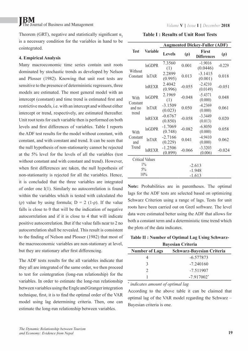
4. Empirical AnalysisMany macroeconomic time series contain unit roots dominated by stochastic trends as developed by Nelson and Plosser (1982). Knowing that unit root tests are sensitive to the presence of deterministic regressors, three models are estimated. The most general model with an intercept (constant) and time trend is estimated first and restrictive models, i.e. with an intercept and without either intercept or trend, respectively, are estimated thereafter. Unit root tests for each variable then is performed on both levels and first differences of variables. Table I reports the ADF test results for the model without constant, with constant, and with constant and trend. It can be seen that the null hypothesis of non-stationarity cannot be rejected at the 5% level for the levels of all the variables (test without constant and with constant and trend). However, when first differences are taken, the null hypothesis of non-stationarity is rejected for all the variables. Hence, it is concluded that the three variables are integrated of order one I(1). Similarly no autocorrelation is found within the variables which is tested with calculated rho (ρ) value by using formula; D = 2 (1-ρ). If the value falls is close to 0 that will be the indication of negative autocorrelation and if it is close to 4 that will indicate positive autocorrelation. But if the value falls near to 2 no autocorrelation shall be revealed. This result is consistent to the finding of Nelson and Plosser (1982) that most of the macroeconomic variables are non-stationary at level, but they are stationary after first differencing.
The ADF tests results for the all variables indicate that they all are integrated of the same order, we then proceed to test for cointegration (long-run relationship) for the variables. In order to estimate the long-run relationship between variables using the Engle and Granger integration technique, first, it is to find the optimal order of the VAR model using lag determining criteria. Then, one can estimate the long-run relationship between variables.
Table I : Results of Unit Root Tests
Test VariableAugmented Dickey-Fuller (ADF)
Levels (ρ) First Differences (ρ)
Without Constant
lnGDPR 7.3560 (1) 0.001 -1.9016
(0.0446) -0.229
lnTAR 2.2899 (0.995) 0.013 -3.1415
(0.001) 0.018
lnREXR 2.4042 (0.996) -0.055 -2.4210
(0.0149) -0.051
With Constant and no trend
lnGDPR 2.1969 (1) -0.048 -5.4371
(0.000) 0.048
lnTAR -3.1509 (0.023) 0.050 -4.2369
(0.000) 0.061
lnREXR -0.6767 (0.850) -0.058 -3.3449
(0.013) 0.020
With Constant
and Trend
lnGDPR -1.7069 (0.748) -0.082 -6.8050
(0.000) 0.058
lnTAR -2.7166 (0.229) 0.041 -4.9410
(0.000) 0.062
lnREXR -1.2506 (0.899) -0.066 -3.3203
(0.006) -0.024
Critical Values1%5%
10%
-2.613-1.948-1.613
Note: Probabilities are in parentheses. The optimal lags for the ADF tests are selected based on optimizing Schwarz Criterion using a range of lags. Tests for unit roots have been carried out on Gretl software. The level data were estimated better using the ADF that allows for both a constant term and a deterministic time trend which the plots of the data indicates.
Table II : Number of Optimal Lag Using Schwarz-Bayesian Criteria
Number of Lags Schwarz-Bayesian Criteria4 -6.5778733 -7.2401602 -7.5119071 -7.917002*
* indicates amount of optimal lagAccording to the above table it can be claimed that optimal lag of the VAR model regarding the Schwarz –Bayesian criteria is one.
The Dynamic Relationship between Tourism and Economy: Evidence from Nepal
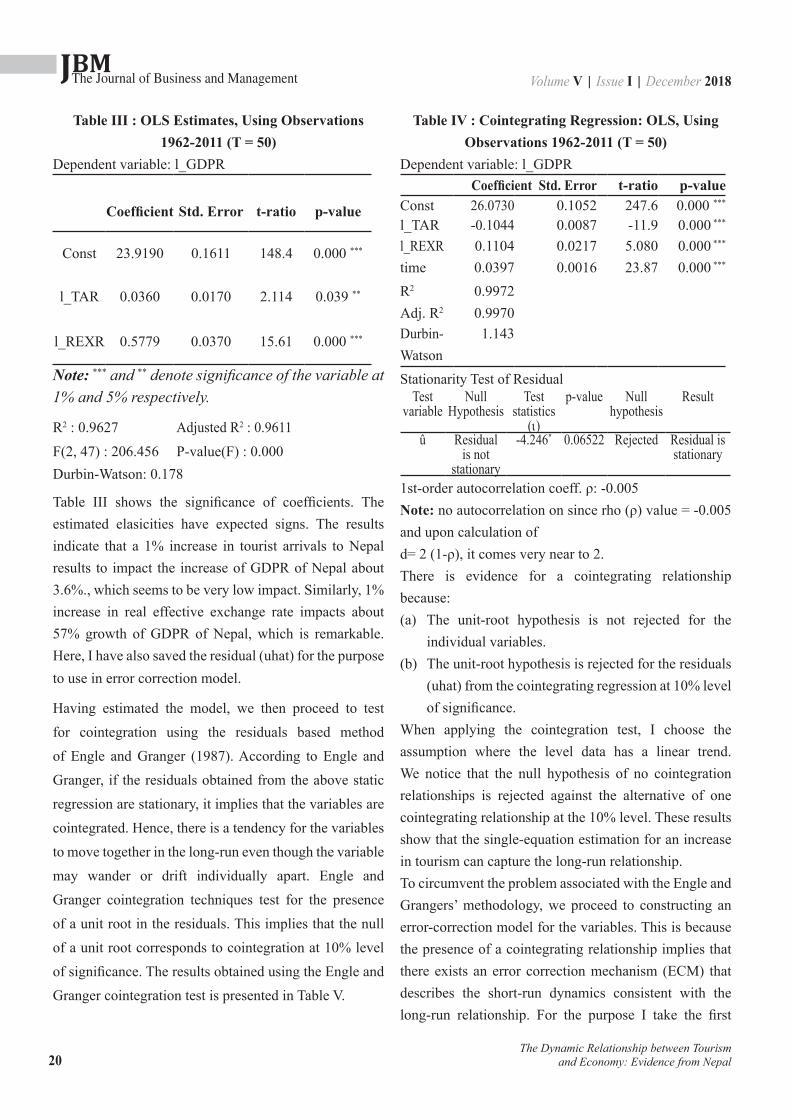
JBMVolume V | Issue I | December 2018The Journal of Business and Management
20
Table III : OLS Estimates, Using Observations 1962-2011 (T = 50)
Dependent variable: l_GDPR
Coefficient Std. Error t-ratio p-value
Const 23.9190 0.1611 148.4 0.000 ***
l_TAR 0.0360 0.0170 2.114 0.039 **
l_REXR 0.5779 0.0370 15.61 0.000 ***
Note: *** and ** denote significance of the variable at 1% and 5% respectively.
R2 : 0.9627 Adjusted R2 : 0.9611
F(2, 47) : 206.456 P-value(F) : 0.000Durbin-Watson: 0.178
Table III shows the significance of coefficients. The estimated elasicities have expected signs. The results indicate that a 1% increase in tourist arrivals to Nepal results to impact the increase of GDPR of Nepal about 3.6%., which seems to be very low impact. Similarly, 1% increase in real effective exchange rate impacts about 57% growth of GDPR of Nepal, which is remarkable. Here, I have also saved the residual (uhat) for the purpose to use in error correction model.
Having estimated the model, we then proceed to test for cointegration using the residuals based method of Engle and Granger (1987). According to Engle and Granger, if the residuals obtained from the above static regression are stationary, it implies that the variables are cointegrated. Hence, there is a tendency for the variables to move together in the long-run even though the variable may wander or drift individually apart. Engle and Granger cointegration techniques test for the presence of a unit root in the residuals. This implies that the null of a unit root corresponds to cointegration at 10% level of significance. The results obtained using the Engle and Granger cointegration test is presented in Table V.
Table IV : Cointegrating Regression: OLS, Using Observations 1962-2011 (T = 50)
Dependent variable: l_GDPRCoefficient Std. Error t-ratio p-value
Const 26.0730 0.1052 247.6 0.000 ***
l_TAR -0.1044 0.0087 -11.9 0.000 ***
l_REXR 0.1104 0.0217 5.080 0.000 ***
time 0.0397 0.0016 23.87 0.000 ***
R2 0.9972Adj. R2 0.9970Durbin- 1.143WatsonStationarity Test of Residual
Test variable
NullHypothesis
Test statistics
(ι)
p-value Null hypothesis
Result
u Residual is not
stationary
-4.246* 0.06522 Rejected Residual is stationary
1st-order autocorrelation coeff. ρ: -0.005Note: no autocorrelation on since rho (ρ) value = -0.005 and upon calculation ofd= 2 (1-ρ), it comes very near to 2.There is evidence for a cointegrating relationship because:(a) The unit-root hypothesis is not rejected for the
individual variables.(b) The unit-root hypothesis is rejected for the residuals
(uhat) from the cointegrating regression at 10% level of significance.
When applying the cointegration test, I choose the assumption where the level data has a linear trend. We notice that the null hypothesis of no cointegration relationships is rejected against the alternative of one cointegrating relationship at the 10% level. These results show that the single-equation estimation for an increase in tourism can capture the long-run relationship.To circumvent the problem associated with the Engle and Grangers’ methodology, we proceed to constructing an error-correction model for the variables. This is because the presence of a cointegrating relationship implies that there exists an error correction mechanism (ECM) that describes the short-run dynamics consistent with the long-run relationship. For the purpose I take the first
The Dynamic Relationship between Tourism and Economy: Evidence from Nepal

JBMVolume V | Issue I | December 2018The Journal of Business and Management
21
difference of the variables and use OLS with the inclusion of u hat and time trend, where u hat has taken lag 1. The results of the ECM are presented in Table V.
Table V : Error Correction Model for Impact of Tourism on Economy
Dependent variable: ∆l_GDPRCoefficient t-ratio p-value
Const 0.01229 1.833 0.0735*
∆l_TAR 0.03721 1.643 0.1076∆l_REXR 0.04302 0.930 0.3573
time 0.00069 4.041 0.000 ***
-0.06330 -2.660 0.0109 **
R2 : 0.1472 Adjusted R2 : 0.0696
Durbin-Watson: 2.631The error correction term _1 is significant and has the expected negative sign. The estimated coefficient of the error correction terms measure the speed of adjustment to restore equilibrium in the dynamic model. According to Table V, the pace of short-run error correction toward equilibrium and long-run state is about -0.063. This clearly indicates that there is a very slow adjustment to the long-run equilibrium i.e. the speed of adjustment rate is about 6.3% for long-run equilibrium between tourism and GDPR.
5. ConclusionThis study investigated empirically the causal nexus between tourism and economic growth. This study also examined the short-run and long-run dynamics of the observed variables for the Nepalese context. Cointegration allows the estimation of long-run equilibrium relationship among economic variables, while ECM permits the modeling of the short-run and the long-run adjustments processes simultaneously. In this paper, I use the cointegration and error correction models to estimate econometric model for economic impact of tourism on Nepal’s economy. This study investigates a series of unit root, cointegration and error correction tests to ascertain whether there is a long-run equilibrium
between gross domestic product, tourist arrivals and real effective exchange rate in Nepal. Using annual data over the 1962-2011 period and since the variables in this paper are nonstationary and present a unit root, Engle and Granger’s cointegration technique is applied. This methodology allowed us to obtain a cointegrating relationship among the three variables. The residual results of ADF test has rejected the null hypothesis of non- stationarity at 10 % significance level and conformed that there is a long-run relationship between the tourism performance and economic growth. It can be claimed that there is a long-run relationship preventing them from diverging over time. In other words, the two variables follow each other over time.
Results of this study provide evidence in favor of ‘demand following’ hypothesis for the Nepalese context. Findings of the study suggest that the there is an important role of tourism performance on economic growth of the country. To the best of my knowledge, this is the first study to undertake both the variables (TAR and REXR) and growth variables (GDP) to study the economic impact of tourism on Nepal’s economy using short-run and long–run dynamics by utilizing 50 years time series data. The main contribution of study is in identifying the role of tourism on economic growth.
Understanding of the relationship between tourism performance and economic growth may assist the researchers, practioners and planners in their estimates of the future planning of the tourism industry. This understanding is of significance for policy makers in developing policies to best suit economic objectives for the country.
A limitation of this study is the inability to account for structural change in the various models. The tourism industry is highly volatile and there is need to account for possibility of structural change in the model building in future study of economic impact of tourism on Nepal’s economy.
The Dynamic Relationship between Tourism and Economy: Evidence from Nepal
JBMVolume V | Issue I | December 2018The Journal of Business and Management
22
References
The Dynamic Relationship between Tourism and Economy: Evidence from Nepal
Balaguer, J. & M. Cantavella-Jorda. (2002). Tourism as a long-run economic growth factor: the Spanish case. Applied Economics, 34, 877-884.
Dickey, D. & W.A. Fuller. (1981). Likelihood ration statistics for autoregressive time series with a unit root. Econometrica, 49, 1057-1072.
Dritsakis, N. (2004). Tourism as a long-run economic growth factor: An empirical investigation for Greece using a causality analysis. Tourism Economics, 10, 305-316.
Durbarry, R. (2004). Tourism and economic growth: the case of Mauritius. Tourism Economics, 10, 389-401.
Enders, W. (2004). Applied Econometric Time Series, 2nd edn, John Wiley & Sons, New Jersey.
Engle, RF & Granger, CWJ. (1987). Cointegration and Error Correction: Representation, Estimation and Testing. Econometrica, 55, 251-276.
Eugenio-Martin, J.L. and N.M., Morales. (2004). Tourism and economic growth in Latin American countries: A panel data approach. Social Science Research Network Electronic Paper.
Granger, CWJ. (1983). Co-Integrated Variables and Error-Correcting Models, Discussion Paper 83-13, University of California, San Diego, CA.
Gunduz, L.& A., Hatemi-J. (2005). Is the tourism-led growth hypothesis valid for Turkey? Applied Economics Letters, 12(8), 499-504.
Johansen, S. (1988). Statistical analysis of cointegrating vectors. Journal of Economic Dynamics Control, 12, 231-254.
Lee, C.C., & C.P., Chang. (2008). Tourism development and economic growth: A closer look at panels. Tourism Management, 29, 180-192.
Nelson, C.R. & C.I., Plosser. (1982). Trends and Random Walks in Macroeconomic Time Series: Some evidence and implications. Journal of Monetary Economics, 10, 139-162.
Oh, C.O. (2005). The contribution of tourism development to economic growth in the Korean economy. Tourism Management, 26, 39-44.
Tang, C.F. (2011). Is the tourism-led growth hypothesis valid for Malaysia? A view from disaggregated tourism markets. International Journal of Tourism Research, 13(1), 97-101.
World Travel & Tourism Council-WTTC. 2011. Nepal: Travel and Tourism Economic Impact, London: WTTC.
Zortuk, M. (2009). Economic Impact of Tourism on Turkey’s economy: Evidence From Cointegration Tests. International Research Journal of Finance and Economics, 25, 231-239.
JBMVolume V | Issue I | December 2018The Journal of Business and Management
23
Digital Financial Literacy: A Study of Households of Udaipur
Hanuman Prasad1, Devendra Meghwal2, Vijay Dayama3
Abstract
Financial literacy has been center of discussion world over. Financial literacy can be generally defined as a person’s ability to understand, analyze, manage, and communicate personal finance matters. More specifically, it refers to the set of skills and knowledge that allows an individual to make informed and effective decisions through their understanding of finances. It is the ability to make informed judgments and take effective decision regarding the use and management of money. Now the trend is change financial literacy become old wine people are moving towards digital financial literacy. The interesting side of digital financial literacy is more people are going of digital payments, the value of internet banking, debit card & credit card, mobile banking are going high. Indian Government is also promoting Digital India recently they have launched many schemes like are Pradhan Mantri Jan Dhan Yojna, Jeevan Jyoti Bima Yojna, Suraksha Bima, MUDRA Bank Yojna, BHIM. The Vittiya Saksharta Abhiyan (VISAKA) also been launched by Ministry of Human Resource. The prime objective of the research is to know the digital financial literacy among the households of Udaipur city. The awareness about various digital platforms and their frequency of use is taken as digital financial literacy. The study further aims to diagnose the impact of personal characteristics on digital financial literacy. The sample of the study is taken from Udaipur city of Rajasthan state of India. A sample of 268 households was selected randomly. A well-structured questionnaire was used to survey and generate digital financial literacy data. The results of study will be a useful direction for both digital platform providers and government to promote citizen for digital transactions. The study also suggests that a wave of awareness campaign is required for bringing more people in the umbrella of digital transaction. Further, a cash transaction oriented economy like India needs to have dual edged sword, where in one hand it needs to bring more policies for lesser use of cash and on the other greater use of digital cash.
Keywords: Digital Financial Literacy, Digital Financial Transactions, Financial InclusionFinancial Literacy
1. Introduction1.1 Digital Financial LiteracyDigital financial literacy has become present need of India. Financial literacy can be generally defined as a person’s ability to understand, analyze, manage, and communicate personal finance matters. More specifically, it refers to the set of skills and knowledge that allows an individual to make informed and effective decisions through their understanding of finances. It is the ability
to make informed judgments and take effective decision regarding the use and management of money. The digital mode of all of this comes in digital financial literacy. Digital financial literacy is directly link or knowledge of online purchasing, online payment through different modes, and online banking system. Digital and cash less India is the mission of present India. The importance of this mission is being felt, especially after the demonetization rollout by Govt. of India Present prime
ISSN 2350-8868
1 Professor, Faculty of Management, MLSU, India2 Research Scholar, Faculty of Management, MLSU, India3 Research Scholar, Faculty of Management, MLSU, India
JBMVolume V | Issue I | December 2018The Journal of Business and Management
24
minister of India has announced on 8th November 2016, the demonetisation of all Rs.500 and Rs.1, 000 banknotes of the Mahatma Gandhi Series. Mahajan and Singla (2017) Indian government adopted demonetization to tackle with black money and make India a cashless digital economy. The demonetization promotes cash-less economy and increase in use of digital financial services. The e-wallet companies have seen a rapid surge in the number of transactions and traffic on their web and app based platforms which are mostly driven by urban and metropolitan parts of the country. Ganiger & B, (2017) India’s present experience of demonetization has revealed the austere digital financial divide of the nation. Millions of people are crowding the banks and queuing outside ATM centers to deposit their cash before the deadline, revealing that India has a long way to go before it fully transitions into a digital financial economy. In spite of expanded digital access to bank accounts, a very small percentage of the population has been able to operate without withdrawing cash or visiting the bank regularly. This is in part due to lower levels of digital Financial literacy. Thus, this makes people to learn the banking mechanisms which not only boosts banking sector but also there can be growth of more literates.However, recently the Government of India and Reserve Bank of India has been pushing the concept and idea of promoting Digital financial Literacy through the help of many campaign.
Recently the Digital Saksharta Abhiyan (DISHA) project sanctioned under the ministry of Electronics and IT, which is being implemented by common service center (CSC), will provide digital financial literacy training and facilitate access to such instruments for one core rural citizens .
The Vittiya Saksharta Abhiyan (VISAKA) also been launched by Ministry of Human Resource. More than 1 lakh students of higher educational institutions have volunteered to be associated with the campaign. The Training will be given to this students and during the training module, students will be trained about the opening of account, linking Aadhaar card with Bank
account, linking Mobile to Aadhaar card and all other required information for digital financial literacy for transforming cash society to less cash society. They will be imparted training in Aadhaar based payment system, pre-paid card, Unified Payments Interface (UPI), Mobile wallet, Unstructured Supplementary Service Data (USSD). As per news publised in The New Indian Express on 13th Dec 2016, National Bank for Agriculture and Rural Development (NABARD) to launch digital financial literacy programmes in Odisha. This kind of activities and schemes are launched to increase digital financial literacy of people. India’s present experience of demonetization has revealed the austere digital financial divide of the nation. Millions of people are crowding the banks and queuing outside ATM centers to deposit their cash before the deadline, revealing that India has a long way to go before it fully transitions into a digital financial economy. In spite of expanded digital access to bank accounts, a very small percentage of the population has been able to operate without withdrawing cash or visiting the bank regularly. This is in part due to lower levels of digital financial literacy. Thus, this makes people to learn the banking mechanisms which not only boosts banking sector but also there can be growth of more literates. The high cost of building and operating bricks and mortar bank branches has been a major obstacles for extending financial services to poor section of society or rural based areas where such facilities cannot been provided. Physical branches are expensive to maintain in far flung communities while traveling to urban areas is costly for many rural customers. However, unbanked individual are increasingly gaining access to financial services through digital channels. Digital finance holds an enormous opportunity for greater financial inclusion and expansion of basic services with the use of mobile phones.
1.2 Financial LiteracyFinancial literacy is become a prominent item on the public agenda worldwide, with its relevance very much underlined by the high-profile role played by consumer finance in global credit crises from 2007 onwards (Williams & Satchell, 2011). Finances are important part
Digital Financial Literacy: A Study of Households of Udaipur
JBMVolume V | Issue I | December 2018The Journal of Business and Management
25
of everyday life and financial literacy is the best way to prevent over-indebtedness of citizens. Tomaskova et.al (2011) financially literate citizens are well versed in issues of money and prices, and are able to manage their personal budget responsibly. Financial literacy helps individuals to improve their level of understanding of financial matters which enables them to process financial information and make apprised decisions about personal finance.
Financial markets around the world have become increasingly accessible to the ‘small investor,’ as new
products and financial services grow widespread (Lusardi & Mitchell, 2013).
Michael et.al (2010) financial literacy is important to understand the basic financial issues that most individuals and families must deal with in our modern society. Even if an individual has a defined benefit plan that will hopefully meet most of the financial needs of one’s retirement years, that person still will spend a lifetime dealing with issues related to mortgages, insurance (including automobile, home, life, and health), personal credit management, income taxes, and all of the other financial considerations that are part of modern life in our society.
One of the causes of Financial Crisis is identified as lack of Financial Literacy. India is a developing country and we are entering into second phase of Financial Sector Reforms. Integration of our economy with world economy will increase further and so the risk of world crisis impacting Indian economy. In India there is large unorganized sector and the Government is withdrawing from pension schemes even in organized sector. In absence of any social security scheme, our economy may be in, for a major instability after demographic dividend starts waning after 20 to 25 years. Thus improvement of financial literacy in the country is
imperative for financial wellbeing of individuals as well as for the economy (Ambarkhane et.al, 2015), The Reserve bank of India, which is the central bank, has been actively participating in the field of eradicating financial literacy
in the country. In this context a project called “Project financial literacy “has already been implemented. (Nash, 2012) Financial literacy in India is on the positive side now. The survey conducted by The Financial Express shows that India has made rapid progress in the field of financial education among the ten leading nations of the world.
India also has been ranked 23rd out of 28 markets in Visa 2012 Global Financial literacy barometer. Financial literacy has gained the attention of a wide range of major banking companies, government agencies, grass-roots consumer and community interest groups, and other organizations. In effective money management can also result in behaviors that make consumers open to severe financial crises. Improved financial literacy can benefit individuals and families by giving them more control over their money and helping them make better financial decisions. (Subha & Priya , 2014)
The Government of India and Reserve bank of India have taken initiatives to spread banking services such as expanding the number of rural bank branches, allowing the banking correspondent model and adoption of CBS technology. While in implementing financial inclusion in a diversified country like India, Financial Literacy plays a pivotal role in the success of this great social initiative opportunity (Shetty & Thomas, 2015).
1.3 Financial InclusionFinancial Inclusion has been center of discussion world over. I.S.T. (2016), even after 60 years of independence, a large section of Indian population still remain unbanked. This malaise has led generation of financial instability and pauperism among the lower income group who do not have access to financial products and services.
The reach of basic financial services to every citizen is known as financial inclusion. The concept of financial inclusion is mostly applicable for that section of society who still does not have access to basic financial services. Thard & Singh (2015), Indian government has done many efforts for financial inclusion. Few among them are Pradhan Mantri Jan Dhan Yojna, Jeevan Jyoti Bima
Digital Financial Literacy: A Study of Households of Udaipur
JBMVolume V | Issue I | December 2018The Journal of Business and Management
26
Yojna, Suraksha Bima, MUDRA Bank Yojna, which was introduced recently.
Guha (2015), hon’ble Prime Minister Mr. Narendra Modi launched programme Pradhan Mantri Jan Dhan Yojana (PMJDY) which was launched on 28 August 2014 with a mission of ensuring access to easy financial services for the excluded section i.e. weaker section and the low income group. As per the scheme one could open an account in any bank branch or Business correspondent outlet with zero balance. The process of opening an account has been made easier. It was an approach to bring about comprehensive financial inclusion of all households in the country. The aim of the scheme is access to banking facilities, financial literacy, and access to credit, insurance and pension facility. Moreover, the beneficiaries would get RuPay Debit card having inbuilt accident insurance covers of Rs. 1 lakh. The plan also envisages channeling all Government benefits to the beneficiaries’ accounts and pushing the Direct Benefits Transfer Scheme of the union Government. The technological issues like poor connectivity, on-line transactions will be addressed. Mobile transactions through telecom operators and their established centers as cash outpoints are also planned to be used for financial Inclusion under the scheme.
1.4 Importance of Digital Financial LiteracyDigital financial literacy is very important in present time as we know that now all financial services and products are available in digital form and present government is also focusing on cash less India and digital India. The importance of digital financial literacy comes in light especially after demonetization. The global revaluation in mobile communication, along with rapid advances in Digital payment system is creating opportunities to connect poor households to affordable and reliable financial tool through mobile phone and other digital interface. Today the unbanked can make use of services that were previously out of rang or not accessible to them.
2. Literature ReviewFinau et.al (2016) examined rural dwellers’ perceptions of digital ªfinancial services (DFS) to identify which factors may enhance or impede their adoption. DFS
are provided by mobile network operators, either individually or in collaboration with commercial banks. The study found that DFS uptake is hindered by agents’ lack of liquidity and the implicit costs that agents impose on consumers. In addition, consumers tend to fully spend the funds received through mobile money, but fail to use their mobile phones for saving purposes. Ghaffar & Sharif (2016) examined the level of financial literacy in Pakistan. The study revealed that the persons, who have more financial knowledge, usually save money. It was found in the study that middle-aged and older people were careful in spending their money and male respondents usually have better saving habits. Further it was also found that respondents earning high salaries agree that financial literacy do help in leading a financially secure life.
Aggarwal and Gupta (2016) identified the linkage between the gender gap in stock market participation and financial literacy while controlling for two major externalities of education level and wealth. It was found that female teachers participate less in stock market to an extent of 16.7% as compared to male. Results of corroborate the view that non-participation in stock markets was a common response to deficiencies in advanced financial literacy and lack of risk attitudes.
Totenhagen et.al (2015) has identified the key considerations and promising delivery methods which may inform positive changes in financial literacy and behavior among youth. Study also has conducted a comprehensive review of the current literature on youth financial literacy education and identified characteristics of financial education programs which influence positive changes.
Hospido et.al (2015) has measured the impact of financial literacy training in compulsory education in Spain. Study used a matched sample of students and teachers in Madrid and two different estimation strategies. It was found in the study that students of private schools did not increase their knowledge much, possibly due to a less intensive implementation of the program. Study also analyzed the bias that arises because the set of schools that participate
Digital Financial Literacy: A Study of Households of Udaipur
JBMVolume V | Issue I | December 2018The Journal of Business and Management
27
in financial literacy programs was not random.
Arif (2015) examined the relationship between financial literacy and the influence of the factors that affect the investment decision. The data was collected from 154 respondents through modified questionnaire containing questions related to demography of the investors, factors affecting the investment decisions and financial literacy level of the individual investors at Karachi Stock Exchange. Study concluded that the financial literacy level of the investors was below average. Significant difference in financial literacy was found between the respondents regarding age, gender, work activity and marital status of the respondents.
Morris and Koffi (2015) has studied the relationship between financial literacy level of Canadian university students and their prior education on the subject. The results revealed that education on financial topics improved financial literacy level. However, the improvement was almost insignificant for courses taken at the secondary level. The results also showed that financial literacy was influenced by socio demographic variables as well.
Potrich et.al (2015) has study the individual financial level through socioeconomic variables. 1400 sample were collected and data analysis was performed by using descriptive statistics and multivariate analysis techniques. Following variable were considered to measure the financial literacy; dependent family members, occupation, educational level, father’s educational level, mother’s educational level, individual income and family income. Results of study were indicating that men who do not have dependent family members and have higher educational and both individual income and family income levels are those who are more likely to belong to the group with high financial literacy levels.
M and M (2015) has examined the financial literacy and its determinants among Gen Y employees in coimbatore city. The study found that gender, education, income and age impact the level of financial literacy. Study also concluded that financial literacy level is low among Gen Y employees in Coimbatore city.
Shih and Ke (2014) has discussed consumer money attitudes, financial literacy regarding financial decisions, and financial behavior. Study suggested that consumers who have retention planning and achievement-esteem attitudes toward money make high-risk financial decisions; anxiety toward money tends to exist mainly in low-risk investors. Financial literacy affects consumer financial behaviors, and demographic variables play segmentation roles.
Park (2011) examined the impact of three dimensions of digital literacy on privacy-related online behaviors: (a) familiarity with technical aspects of the Internet, (b) awareness of common institutional practices, and (c) understanding of current privacy policy. Hierarchical regression models analyzed data from a national sample of 419 adult Internet users. The analyses showed strong predictive powers of user knowledge, as indicated by the three discrete dimensions, on privacy control behavior.
Way & Wong (2010) state that the development and use of technology-based tools for financial literacy education has grown rapidly in recent years, often based on the presumption that digital media will enhance past practice. The studies present an ecological model for technology-based financial literacy education intervention and propose an action agenda for practice and further research.
3. Data and Methodology The study aims to map digital financial literacy among the house holds of Udaipur city of Rajasthan state of India. The study has employed descriptive survey research design. A questionnaire consisting of instrument to map the frequency of use of digital platform for financial transactions in form of 11 statements related to variety of expenditures and investments was developed. Similarly one more instrument mapping the awareness about availability of digital platforms was inserted.
After a pilot survey and incorporating suggestions of a penal of experts to establish content validity, the questionnaire was administered on 300 households of Udaipur (Rajasthan), out of which 32 responses were excluded due insufficient information. Finally, the 268
Digital Financial Literacy: A Study of Households of Udaipur
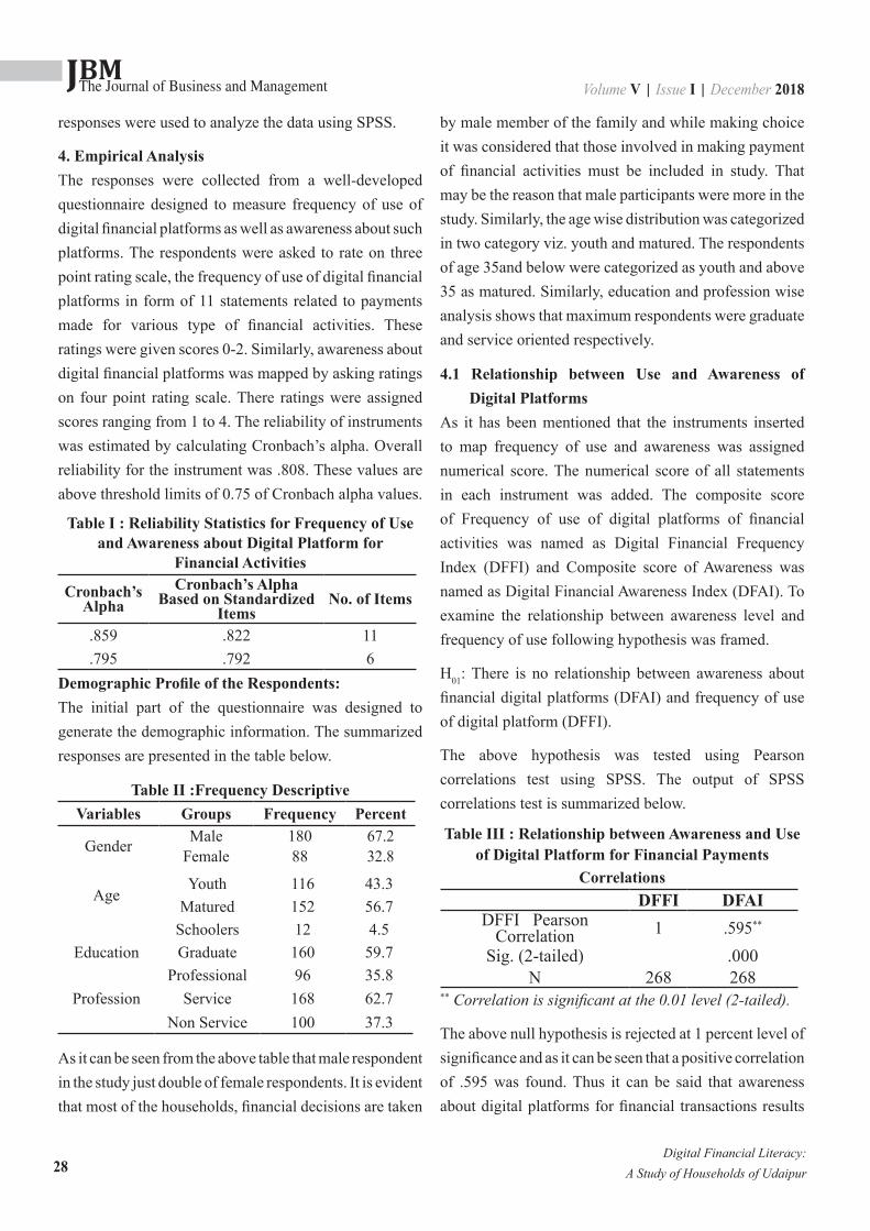
JBMVolume V | Issue I | December 2018The Journal of Business and Management
28
responses were used to analyze the data using SPSS.
4. Empirical AnalysisThe responses were collected from a well-developed questionnaire designed to measure frequency of use of digital financial platforms as well as awareness about such platforms. The respondents were asked to rate on three point rating scale, the frequency of use of digital financial platforms in form of 11 statements related to payments made for various type of financial activities. These ratings were given scores 0-2. Similarly, awareness about digital financial platforms was mapped by asking ratings on four point rating scale. There ratings were assigned scores ranging from 1 to 4. The reliability of instruments was estimated by calculating Cronbach’s alpha. Overall reliability for the instrument was .808. These values are above threshold limits of 0.75 of Cronbach alpha values.
Table I : Reliability Statistics for Frequency of Use and Awareness about Digital Platform for
Financial Activities
Cronbach’sAlpha
Cronbach’s AlphaBased on Standardized
ItemsNo. of Items
.859 .822 11
.795 .792 6Demographic Profile of the Respondents:The initial part of the questionnaire was designed to generate the demographic information. The summarized responses are presented in the table below.
Table II :Frequency DescriptiveVariables Groups Frequency Percent
Gender Male 180 67.2Female 88 32.8
AgeYouth 116 43.3
Matured 152 56.7
EducationSchoolers 12 4.5Graduate 160 59.7
Professional 96 35.8Profession Service 168 62.7
Non Service 100 37.3
As it can be seen from the above table that male respondent in the study just double of female respondents. It is evident that most of the households, financial decisions are taken
by male member of the family and while making choice it was considered that those involved in making payment of financial activities must be included in study. That may be the reason that male participants were more in the study. Similarly, the age wise distribution was categorized in two category viz. youth and matured. The respondents of age 35and below were categorized as youth and above 35 as matured. Similarly, education and profession wise analysis shows that maximum respondents were graduate and service oriented respectively.
4.1 Relationship between Use and Awareness of Digital Platforms
As it has been mentioned that the instruments inserted to map frequency of use and awareness was assigned numerical score. The numerical score of all statements in each instrument was added. The composite score of Frequency of use of digital platforms of financial activities was named as Digital Financial Frequency Index (DFFI) and Composite score of Awareness was named as Digital Financial Awareness Index (DFAI). To examine the relationship between awareness level and frequency of use following hypothesis was framed.
H01: There is no relationship between awareness about financial digital platforms (DFAI) and frequency of use of digital platform (DFFI).
The above hypothesis was tested using Pearson correlations test using SPSS. The output of SPSS correlations test is summarized below.
Table III : Relationship between Awareness and Use of Digital Platform for Financial Payments
CorrelationsDFFI DFAI
DFFI PearsonCorrelation 1 .595**
Sig. (2-tailed) .000N 268 268
** Correlation is significant at the 0.01 level (2-tailed).
The above null hypothesis is rejected at 1 percent level of significance and as it can be seen that a positive correlation of .595 was found. Thus it can be said that awareness about digital platforms for financial transactions results
Digital Financial Literacy: A Study of Households of Udaipur
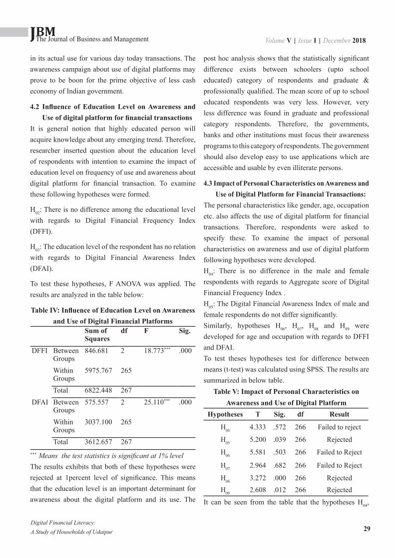
JBMVolume V | Issue I | December 2018The Journal of Business and Management
29
in its actual use for various day today transactions. The awareness campaign about use of digital platforms may prove to be boon for the prime objective of less cash economy of Indian government.
4.2 Influence of Education Level on Awareness and Use of digital platform for financial transactions
It is general notion that highly educated person will acquire knowledge about any emerging trend. Therefore, researcher inserted question about the education level of respondents with intention to examine the impact of education level on frequency of use and awareness about digital platform for financial transaction. To examine these following hypotheses were formed.
H02: There is no difference among the educational level with regards to Digital Financial Frequency Index (DFFI).
H03: The education level of the respondent has no relation with regards to Digital Financial Awareness Index (DFAI).
To test these hypotheses, F ANOVA was applied. The results are analyzed in the table below:
Table IV: Influence of Education Level on Awareness and Use of Digital Financial Platforms
Sum of Squares
df F Sig.
DFFI Between Groups
846.681 2 18.773*** .000
Within Groups
5975.767 265
Total 6822.448 267DFAI Between
Groups575.557 2 25.110*** .000
Within Groups
3037.100 265
Total 3612.657 267*** Means the test statistics is significant at 1% level The results exhibits that both of these hypotheses were rejected at 1percent level of significance. This means that the education level is an important determinant for awareness about the digital platform and its use. The
post hoc analysis shows that the statistically significant difference exists between schoolers (upto school educated) category of respondents and graduate & professionally qualified. The mean score of up to school educated respondents was very less. However, very less difference was found in graduate and professional category respondents. Therefore, the governments, banks and other institutions must focus their awareness programs to this category of respondents. The government should also develop easy to use applications which are accessible and usable by even illiterate persons.
4.3 Impact of Personal Characteristics on Awareness and Use of Digital Platform for Financial Transactions:
The personal characteristics like gender, age, occupation etc. also affects the use of digital platform for financial transactions. Therefore, respondents were asked to specify these. To examine the impact of personal characteristics on awareness and use of digital platform following hypotheses were developed.H04: There is no difference in the male and female respondents with regards to Aggregate score of Digital Financial Frequency Index .H05: The Digital Financial Awareness Index of male and female respondents do not differ significantly.Similarly, hypotheses H06, H07, H08 and H09 were developed for age and occupation with regards to DFFI and DFAI.To test theses hypotheses test for difference between means (t-test) was calculated using SPSS. The results are summarized in below table.
Table V: Impact of Personal Characteristics on Awareness and Use of Digital Platform
Hypotheses T Sig. df Result
H04 4.333 .572 266 Failed to reject
H05 5.200 .039 266 Rejected
H06 5.581 .503 266 Failed to Reject
H07 2.964 .682 266 Failed to Reject
H08 3.272 .000 266 RejectedH09 2.608 .012 266 Rejected
It can be seen from the table that the hypotheses H04,
Digital Financial Literacy: A Study of Households of Udaipur
JBMVolume V | Issue I | December 2018The Journal of Business and Management
30
H06, H08 were related to DFFI (frequency of use). The hypothesis related with occupation H08 was rejected at one percent level of significance while the test failed to reject the rest two hypotheses related with age and gender. Which means that statistical difference in use of digital platforms exist in service and non-service class of occupation. The mean score of service class was found more. It may be due to the fact that service class people have disclosed money thus they do not hesitate in doing transaction through digital platform.
The hypotheses H05, H07 and H09 were related to awareness about digital platform. The hypotheses related with gender and occupation was rejected at 5 percent level of significance. The mean score of male participants was higher as compared to females. It may be due to the fact that females particularly of matured age have less exposure to digital platform. Therefore, awareness programs for female households regarding digital platforms need to be undertaken. The statistically significant difference in awareness about digital platforms exists in service and non-service category. The awareness means score of non-service category was less as compared to service category.
The non-service category has less mean score of awareness as well as utilization of digital financial platforms (DFFI and DFAI). Therefore, it may also be inferred that non service respondents do not use digital platform due to non-awareness. Thus awareness programs for such non service class people must be arranged.
5. ConclusionThe study aims was to map digital financial literacy among the house holds of Udaipur city of Rajasthan state of India. The study has employed descriptive survey research design. A questionnaire consisting of instrument to map the frequency of use of digital platform for financial transactions in form of 11 statements related to variety of expenditures and investments was developed. Similarly one more instrument mapping the awareness about availability of digital platforms was inserted. The
questionnaire was administered on 300 households of Udaipur (Rajasthan). Out of which 32 responses were excluded due insufficient information. From the findings of the research it can be said that male of households were more familiar with digital financial platforms and more aware. Similarly, the age wise distribution was categorized in two category viz. youth and matured. The respondents of age 35and below were categorized as youth and above 35 as matured. Similarly, education and profession wise analysis shows that maximum respondents were graduate and service oriented respectively. Frequency of use of digital platforms of financial activities was named as Digital Financial Frequency Index (DFFI) and Composite score of Awareness was named as Digital Financial Awareness Index (DFAI).
It was found that the education level is an important determinant for awareness about the digital platform and its use. The mean score of up to school educated respondents was very less. However, very less difference was found in graduate and professional category respondents. Therefore, the governments, banks and other institutions must focus their awareness programs to this category of respondents. The government should also develop easy to use applications which are accessible and usable by even illiterate persons. It was also found that the statistical difference in use of digital platforms exist in service and non-service class of occupation. The mean score of service class was found more. It may be due to the fact that service class people have disclosed money thus they do not hesitate in doing transaction through digital platform. Therefore, it may also be inferred that non service respondents do not use digital platform due to non-awareness. Thus awareness programs for such non service class people must be arranged. The mean score of male participants was higher as compared to females. It may be due to the fact that females particularly of matured age have less exposure to digital platform. Therefore, awareness programs for female households regarding digital platforms need to be undertaken
Digital Financial Literacy: A Study of Households of Udaipur

JBMVolume V | Issue I | December 2018The Journal of Business and Management
31
Aggarwal, D., & Gupta, D. (2014). Awareness of Financial Literacy Among College Students. Journal of Management Sciences and Technology, 2(1), 1-13.
Ambarkhane, D., Venkataramani, B., & Singh, A. S. (2015). Financial Literacy Index For College Students. Annual Research Journal of Symbiosis Centre For Management Studies, 3, 1-25.
Arif, K. (2015). Financial Literacy and Other Factors Influencing Individuals’Investment Decision: Evidence From A Developing Economy. Journal of Poverty, Investment And Development, 12, 74-84.
Finau, G., Rika, N., Samuwai, J., & Mcgoon, J. (2016). Perceptions of Digital Financial Services in Rural Fiji. Information Technologies & International Development, 12(4), 11-21.
Ganiger, V. S., & B, R. (2017). Demonetisation and its impact on social development. Indian journal of applied research, 7(1), 770-771.
Guha, S. (2015). The Role of Pradhan Mantri Jan Dhan Yojana in Financial Inclusion: An Evaluative Study. GJRA - Global Journal for Research Analysis, 4(7), 361-362.
Ghaffar, S., & Sharif, S. (2016). The Level Of Financial Literacy In Pakistan. Social Scince Research Netwok, Retrieved from http://Ssrn.Com/Abstract=2724533, 1-29.
Hospido, L., Villanueva, E., & Zamarro, G. (2015). The Impact of Financial Literacy Training In The Impact of Financial Literacy Training In. IZA Discussion Paper No. 8902, 1-44. I, S. T. (2016). International Education & Research Journal [IERJ], 2(12), 17-19.
Lusardi, A., & Mitchell, O. S. (2013). The Economic Importance of Financial Literacy: Theory and Evidence. Journal of Economic Literature, 52(1), 5-44.
M, S., & M, G. (2015 ). A Study on Financial Literacy and Its Determinants Among Gen Y Employees In Coimbatore City. Great Lakes Herald, 9(1), 35-45.
Mahajan, P., & Singla, A. (2017). Effect of demonetization on financial inclusion in India, International Conference on Recent Trends in Engineering, Science & Management, 1282-1287.
Michael , H. E., Hill, R. R., & Perdue, G. (2010). School of Study and Financial Literacy. Journal of Economics and Economic Education Research, 11(3), 29-37.
Morris, T., & Koffi , V. (2015). The Link Between Financial Literacy and Education of Canadian University Students. International Journal of Innovation and Research In Educational Sciences, 2(3), 160-170.
Nash, D. R. (2012). Financial Literacy: An Indian Scenario. Asian Journal of Research In Banking and Finance , 2(4), 70-84.
Park, Y. J. (2011). Digital Literacy and Privacy Behavior Online. Communication Research, 40(2), 215-236.
Press Information Bureau. (2017). Retrieved on Feb 14, 2017, from http://pib.nic.in/newsite/ PrintRelease.aspx?relid=155462
Potrich, A. C., Vieira, M. K., & Kirch, G. (2015). Determinants of Financial Literacy: Analysis of The Influence of Socioeconomic and Demographic Variables. Revista Contabilidade & Finanças, 26(69), 362-377.
Digital Financial Literacy: A Study of Households of Udaipur
References
JBMVolume V | Issue I | December 2018The Journal of Business and Management
32
Shetty, D. S., & Thomas, B. J. (2015, March). A Study of Financial Literacy Amongst The College Students In Mumbai. Tactful Management Research Journal, 6, 6-11.
Shih, T. Y., & Ke, S. C. (2014). Determinates of financial Behavior: Insights Into Consumer Money Attitudes and financial Literacy. Service Business, 8, 217-238.
Subha, D. V., & Priya , P. S. (2014 ). A Study On The Factors Determining Financial Literacy of Households. International Journal of Advanced Information Science and Technology, 22(22), 15-20.
Thard , N., & Singh, J. (2015). Financial Inclusion A Key to Micro Finance. Indian Journal of Appled Reasarch, 5(11), 134-136.
Tomaskova, H., Mohelska, H., & Nemcova, Z. (2011). Issues of Financial Literacy Education. Procedia - Social and Behavioral Sciences, 28, 365-369.
Totenhagen, C. J., Deborah, C. M., Faber, K. M., Bosch, L. A., Wiggs, C. B., & Lynne , B. M. (2015). Youth Financial Literacy: A Review of Key Considerations and Promising Delivery Methods. J Fam Econ Iss, 36, 167-191.
Way, W. L., & Wong, N. (2010). Harnessing the Power of Technology to Enhance Financial Literacy Education and Personal Financial Well-Being: A Review of the Literature, Proposed Model, and Action Agenda. Center for Financial Security WP, 1-100.
Williams , O. J., & Satchell, S. E. (2011). Social Welfare Issues of financial Literacy And Their Implications For Regulation. Journal of Regulatory Economics, 40(1), 1-39.
Digital Financial Literacy: A Study of Households of Udaipur
JBMVolume V | Issue I | December 2018The Journal of Business and Management
33
Market Structure and Performance of Commercial Banks: Empirical Evidence from Nepal
Kripa Kunwar1
Abstract
The study attempts to examine the relationship of market structure variable with the performance of Nepalese commercial banks over the period 2011-2015 using causal research design. The stratified sampling technique has been employed to select sample banks which include 10 commercial banks comprising 5 joint venture and 5 local private banks. A pooled OLS model is specified, and then the indicators of market structure are used as explanatory variables in the regression model. Study results have shown that market concentration has had a negative and significant impact on the performance of the Nepalese commercial banks. Where the Herfindahl-Hirschman index (HHI) is used the market shares as the main variable to measure the concentration (CONC). Empirical results revealed that lower the market concentration higher will be the performance of the bank. On the other hand, study concluded that market power has positive influence on profitability. The Data Envelopment Analysis (DEA) method was used to assess the efficiency scores. On the contrary, empirical results indicated that there is no relationship between the bank’s efficiency and performance in Nepalese commercial banks. As far as the ownership structure is concerned, study found that, ROA differences depend on bank ownership types. Study concluded that performance of the joint venture banks is better than local private banks in sample period.
Keywords: Bank Efficiency, Bank Performance, Market Power, Market Structure
1. IntroductionMarket structure of the banking industry refers to the number of banks in the market, their market share and other features which affect the level of competition in the market. As well as market structure influences the bank’s behavior whether it is efficient, and level of profits it can generate. Considering market structures, modern theory also looks at the firm’s performance and the level of contestability in the market. The theory of Market Power (MP) and the theory of Efficient Structure (ES) explain the relationship between the market structure and performance of the bank. Furthermore, Structure-Conduct-Performance hypothesis (SCP) and Relative Market Power hypothesis (RMP) are concerned with MP theory similarly x-efficiency (XE) and scale efficiency (SE) hypothesis explain the ES theory.
Under structure conduct performance (SCP) analyzing
paradigm, the market structure affects performance. Fu and Heffernan (2009), Ayadi & Ellouze (2013) explain that according to SCP hypothesis the more concentrated the banking system, the more it is able to earn higher profits and thereafter the more it efficient will be. Under RMP hypothesis the banks with a large market share and diversified products that might exercise their market power to determine prices and make profits. As a result, individual market shares accurately determine market power and market imperfections (Mensi & Zouari, 2010). Berger (1995), Mensi & Zouari (2010) explain that under the x-efficiency hypothesis, the costs incurred by banks with efficient management and/or technologies are lower resulting in higher profitability. The better banks x-efficiency is, larger are market shares and higher is concentration. Under the efficiency hypothesis, the difference in performance between two firms is not due to differences in management quality, but to differences at
1Lecturer, School of Business, Pokhara University
ISSN 2350-8868
JBMVolume V | Issue I | December 2018The Journal of Business and Management
34
the level of scale efficiency. Banks costs lower than their competitors result in higher profitability. These banks may acquire extended market shares which increases market concentration.
The history of modern banking practices in Nepal has started after the establishment of Nepal bank Limited in the year 1937. Similarly Nepalese financial system got the new dimension after the establishment of Nepal Rastra Bank as the central bank in the year 1956. With the initiation of financial sector liberalization process during 1980s many joint venture and local private banks entered into the market. Banking industry of Nepal has been characterized by strong competition with the continual increase in the number of banks. After the entry of joint venture banks and then the mushrooming of Nepalese private banks with the new definition of and approach to banking, the whole banking industry in general, and the one-time monopolist government-owned banks in particular are under the pressure to continue their competitive position (Thapa, 2010). As the apex body of financial institution, Nepal Rastra bank (NRB) regulates the activities of financial institution; provide guidelines and suggestion to make them more competitive and efficient. Under the policy adopted by NRB many banks which are operating in Nepal are going for merger and acquisition. As on October 2016, there are 28 commercial banks in Nepal. Out of these 7 are joint venture banks and 3 are state-owned and remaining are local private bank.
Financial system of Nepal is highly dominated by banking sector, particularly commercial banks. As a result the economic stability and growth of the country largely depend on the banking industry. That’s why the policy should focus on banking sector development by enhancing its quality in Nepal (Kharel & Pokhrel, 2012). Market structure of the bank is long consider as the main factor for the development of banking industry that influences the competitiveness of the banking system and companies’ access to funding and thereby their investment (González, 2009).
Pradhan and Gajurel (2011) concluded that Nepalese banking industry is becoming less concentrated and more competitive in recent years. Scenario of banking industry in Nepal is ever changing due to the changing government policy. As a result performances of the banks are affected. This study has been designed to examine the structure-performance relationship of the Nepalese commercial banks. There have been extensive research works on the relationship between
Market Structure and Performance of the bank. Review of large number of previous studies suggests that market structure of banking industry can influence the performance of the banks. Similarly past studies and theory recommend that efficiency and market structure are the key factors for the survival in complex environment in banking industries where market concentration and market share are regarded as the index of market structure of the bank. Herfindahl-Hirshman index (HHI) is used to measure the market concentration and competitiveness (Ayadi & Ellouze, 2013). Likewise Data Envelopment Analysis (DEA) method is used to assess the efficiency scores. Looking at current scenario of Nepalese banking industry, the present study has raised the following research question:
i. Is there a relationship between market structure variable and performance of commercial banks?
On the basis of the above mentioned background and statement of the problem following objective has been set for the study:i. To examine the relationship of market structure
variable with the performance of commercial banks.
2. Literature ReviewTan and Floros (2013) examined the relationship between (i) risk and market power, and (ii) efficiency/ productivity and market power. Study reveals that higher efficiency leads to higher market power for Chinese banks. Furthermore, researcher found that Chinese banks with higher volumes of nontraditional activities normally have lower market power.
Market Structure and Performance of Commercial Banks: Empirical Evidence from Nepal
JBMVolume V | Issue I | December 2018The Journal of Business and Management
35
Ayadi and Ellouze (2013) tested the theory of Market Power (MP) and the theory of Efficient Structure (ES) to explain the relationship between bank performance and market structure. Regarding the theory of MP, it includes two hypotheses: Structure-Conduct-Performance hypothesis (SCP) and Relative Market Power hypothesis (RMP). With regard to the theory (ES), it has also two hypotheses: the hypothesis of x -efficiency (ESX) and the hypothesis of scale efficiency (ESS). And Results showed that x-efficiency has had a positive and significant effect on the performance of the Tunisian commercial banks as well as the hypothesis of x-efficiency.
Zhengchao and Qin (2012) analyzed the relationship between Chinese banking market structure and performance. Researcher employed the methodology of SCP (structure-conduct-performance), introduce macro economics factors into regression model and use the panel data of 14 major commercial banks in China Mainland from 2000 to 2010. The results showed that China banking market is still in the oligopoly status, and the oligopoly degree reduces gradually over time. The oligopoly degree has a negative correlation with the performance which was measured by Herfindahl-Hirschman Index ( HHI ). The deposit-loan ratio and the capital adequacy ratio have both positive correlations with the performance.
Ugwunta, Ani, Ugwuanyi, and Ugwu (2012) measured the market structure and competition in the consolidated Nigerian banking industry, as well as investigated the impact of the banking sector structure on bank performance. Significant findings included that the Nigerian banking sector is oligopolistic in structure and that market concentration positively and significantly impacts on bank performance. These results suggested that market concentration is a major determinant of bank profitability in Nigeria.
Pradhan and Gajurel (2011) tested the structure performance hypotheses in the context of Nepalese banking industry for the period of 2001-2009 under the Berger and Hannan (1993) empirical framework. The empirical results suggested that traditional structure-
conduct-performance hypothesis and quite life hypothesis are better explaining concentration-profitability relation in Nepalese banking industry. Similarly study found that there is weak support for efficiency structure hypotheses.
Thapa (2010) examined strategy-performance relationship in the Nepalese banks. The findings of this study have suggested that there exists a positive relationship between competitive strategies pursued by the banks and their organizational performance. The highest performance seemed to be correlated with cost leadership (cost reduction, operating efficiency and offering competitive prices) strategy, followed by differentiation (in particular through unique and wider range of services offered) strategy, and market-focus strategy respectively. It is further observed that banks have preferred more to pursue the combination of cost-leadership and differentiation strategies than the market-focus strategy to attain their higher performance.
Mensi and Zouari (2010) investigated the market structure-performance relationship within the Tunisian banking system. They distinguished between two theories, namely the Efficient Structure Theory and Market Power Theory using the Data Envelopment Analysis Method, and estimated efficiency measures under X-efficiency, Technical Efficiency, Scale Efficiency and Allocative Efficiency. The empirical investigation is conducted on profit and price regressions for a sample of 10 commercial banks. The results rejected the SCP and Quite life hypotheses under the market power theory but retain the RMP hypotheses. Also, all the hypotheses under Efficient Structure theory are rejected.
3. Hypotheses DevelopmentThe theory of Market Power (MP) and the theory of Efficient Structure (ES) explain the relationship between market structure and performance of the bank. Regarding the theory of MP, it includes two hypotheses: Structure-Conduct-Performance hypothesis (SCP) and Relative Market Power hypothesis (RMP) (Ayadi Ellouze, 2013). Similarly ES theory also includes two hypothesis x-efficiency and scale efficiency. According to structure conduct performance (SCP) analyzing paradigm, the
Market Structure and Performance of Commercial Banks: Empirical Evidence from Nepal
JBMVolume V | Issue I | December 2018The Journal of Business and Management
36
market structure affects performance. Ayadi & Ellouze (2013) explain that under SCP hypothesis the more concentrated the banking system, the more it is able to earn higher profits. Herfindahl-Hirschman Index (HHI) can reflect the comprehensive condition of the whole banking industry that represents market structure. Moreover, the market concentration rate is usually utilized to represent market structure (Zhengchao & Qin, 2012). Bamakhramah (1992) observed a negative correlation between the concentration level and profitability rates in the banking system of Saudi Arabia. Bhatti & Hussain (2010) Using regression analysis, they found a positive relationship between concentration ratio (CR) and profitability in Pakistani commercial banks. On the basis of previous research, study set the first hypothesis to find out the relationship between Bank concentrations with bank performance.
H1: Bank concentration is positively related with bank performance.
From the past studies, market share is one of the important variables that affect the profitability of the firm. Market share is regarded as the index of market structure of the bank. RMP hypothesis states that the banks with relatively larger market share and a range of differentiated product lines are better able to exercise their market power to gain superior profit. RMP emphasize excess profit deriving from larger banks’ individual market share but not necessarily from collusive behaviors (Pradhan & Gajurel, 2011). The study develops the hypothesis on the following manner to support the objective of the study.
H2: There is positive relationship between market share and performance of the bank.
Furthermore Efficient Structure (ES) theory also includes two hypothesis x-efficiency and scale efficiency. X-efficiency hypothesis explain that market concentration is resulted from the efficiency of the bank. Consequently, bank’s higher profit is derived from operational efficiency. Similarly The scale efficiency hypothesis, emphasize more on the level of scale economies. The banks operating at scale efficient level have lower cost per unit which helps to increase profitability. Pradhan & Gajurel (2011)
found that there is weak support for efficiency structure hypotheses. Tan & Floros (2013) reveals that higher efficiency leads to higher market power for Chinese banks. The study examines the following hypothesis on the base of the theories and past studies.
H3: There is positive relationship between efficiency score and performance.
There are many existing studies that investigate the effects of foreign ownership on the efficiencies or stabilities of host country banking industry (Claessens, et al., 2000; Claeys & Hainz, 2007). Many cross-country and case studies, suggest that foreign banks are more efficient than their domestic competitors in developing countries (O’Sullivan, 2012). It is pointed out that foreign ownership could help to increase the soundness and stability of the banking system of the host country because foreign banks are known to have superior business resources and strategies and conduct more active and aggressive risk management and stability oriented businesses. Ownership structure is measured by dummy variable taking value of 0 for foreign joint venture banks and 1 for local private banks in this research study. This study is going to test the following hypothesis on the basis of previous literature.
H4: Foreign ownership positively impacts bank performance.
4. Data and MethodologyThe study attempts to empirically investigate the relationship between market structure and performance of the Nepalese commercial banks over the study period of 2011-2015 using causal research design. The study is based on secondary source of data obtained from published annul reports of the sample banks. The stratified sampling technique has been employed to select sample banks which include 10 commercial banks comprising 5 joint venture and 5 local private banks. The public sector banks have been excluded from the study. The purposively selected joint venture banks are Everest bank Limited (EBL), Nepal SBI bank (NSBI), Nabil bank (NABIL), Nepal Bangladesh bank (NBBL), and Himalyan bank Limited (HBL). Similarly
Market Structure and Performance of Commercial Banks: Empirical Evidence from Nepal

JBMVolume V | Issue I | December 2018The Journal of Business and Management
37
local private banks are Nepal investment bank (NIB), Laxmi Bank (LBL), Kumari Bank (KBL), Sunrise bank Limited (SUNBL) and Siddhartha bank Limited (SBL). To examine the relationship between banking market structure and performance, a pooled OLS model is specified, and then the indicators of market structure are used as explanatory variables in the regression model. The regression model used in the study has the following specification:ROAi,t= α0 + β1 CONCi,t + β2 MSi,t + β3 ESi,t + β4 OWNi,t
+ εi,t ................ (1)Where, ROA is the dependent variable representing bank performance. CONC is market performance measured by Herfindahl Hirschman Index (HHI), MS is market share in terms of deposits, ES is efficiency score computed using DEA and OWN is a dummy variable representing joint venture banks with foreign ownership and local private banks with dichotomous value of 0 and 1 respectively. The subscript i represents ith bank and the subscript t represents tth year in the study period. εit is the residual error.
Bank Efficiency MeasureData Envelopment analysis (DEA) is used in the study which is non-parametric approach based on sample data to measure the efficiency of sample banks. DEA has proven to be a popular technique for efficiency analysis in general, and in the financial services industry in particular. DEA optimizes on each individual observation with the objective of calculating a discrete piecewise linear frontier determined by the set of Pareto-efficient decision making units (DMUs) which are the sample A-class financial institutions in the study. Using this frontier, DEA computes a maximal performance measure for each DMU relative to all other DMUs. The study uses CCR input-oriented variable returns to scale DEA model to reduce the multiple-input, multiple-output situation for each bank to a scalar measure of efficiency. Staff expenses and interest expenses are taken as inputs while investment and loan are taken as output for the purpose of this analysis. Efficiency scores vary between 0 and 1, with 1 representing fully efficient DMU. The efficiency scores are calculated as follows:
max EFFk = (∑urkyrk)/( ∑vikxik) .........(2)Subject to : (∑urkyrj)/( ∑vikxij)< 1; j = 1, ...,n.
∑urk > ∈; r =1, ...,s.∑vik >∈; i =1,...,m.
∈ > 0. Where max EFFk means maximize efficiency of bank k. This model evaluates the relative efficiency of bank k based on the performance of j=1,...,n banks in the population, where the yrj and xij variables in the model represent the observed amounts of the rth output and the ith input, respectively, of the jth bank.
Herfindahl-Hirschman Index (HHI)HHI is the most widely used measure of concentration and a proxy for competition in theoretical research and empirical analysis. It is the sum of the squares of market shares of all the banks and has the following form:
HHIt=N 2i=1 it∑ S .........(3)
Where, Sit is the market share of bank i in year t and N is the total number of banks in the system. In calculating market shares, total assets have been taken as a measure of bank size. Contrary to the n-bank concentration ratios, in the calculation of HHI, all banks in the market are taken into account. HHI stresses the importance of larger banks by giving them a higher weight than smaller banks. Larger value of HHI indicates larger concentration or less competition and vice-versa.
5. Empirical AnalysisAs far as the bank efficiency is concerned, the study focus on the DEA efficiency scores of Nepalese commercial banks in our sample, then the structure –performance relationship is analyzed latter for the period 2011-2015. The mean values of efficiency scores are presented in Table I.Table I shows the sampled 10 commercial bank’s respective average efficiency score. Average efficiency score of the sample banks during the period 2011-2015 is estimated at 0.86178. This result reflected that inefficiency cost is on average around 0.138282 that indicates a waste of resources in the Nepalese banks which is very low.
Market Structure and Performance of Commercial Banks: Empirical Evidence from Nepal
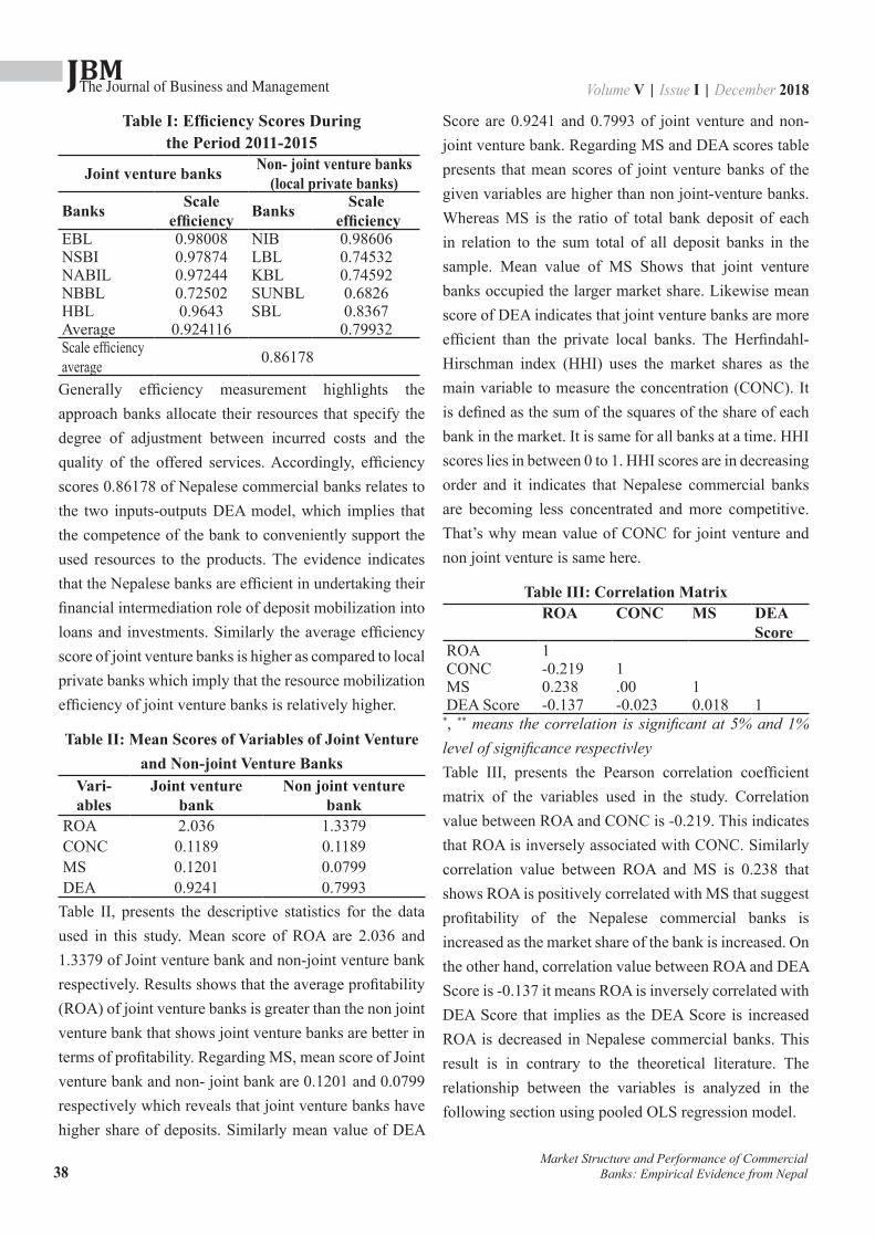
JBMVolume V | Issue I | December 2018The Journal of Business and Management
38
Table I: Efficiency Scores During the Period 2011-2015
Joint venture banks Non- joint venture banks (local private banks)
Banks Scale efficiency Banks Scale
efficiency EBL 0.98008 NIB 0.98606NSBI 0.97874 LBL 0.74532NABIL 0.97244 KBL 0.74592NBBL 0.72502 SUNBL 0.6826HBL 0.9643 SBL 0.8367Average 0.924116 0.79932Scale efficiency average 0.86178
Generally efficiency measurement highlights the approach banks allocate their resources that specify the degree of adjustment between incurred costs and the quality of the offered services. Accordingly, efficiency scores 0.86178 of Nepalese commercial banks relates to the two inputs-outputs DEA model, which implies that the competence of the bank to conveniently support the used resources to the products. The evidence indicates that the Nepalese banks are efficient in undertaking their financial intermediation role of deposit mobilization into loans and investments. Similarly the average efficiency score of joint venture banks is higher as compared to local private banks which imply that the resource mobilization efficiency of joint venture banks is relatively higher.
Table II: Mean Scores of Variables of Joint Venture and Non-joint Venture Banks
Vari-ables
Joint venture bank
Non joint venture bank
ROA 2.036 1.3379CONC 0.1189 0.1189MS 0.1201 0.0799DEA 0.9241 0.7993
Table II, presents the descriptive statistics for the data used in this study. Mean score of ROA are 2.036 and 1.3379 of Joint venture bank and non-joint venture bank respectively. Results shows that the average profitability (ROA) of joint venture banks is greater than the non joint venture bank that shows joint venture banks are better in terms of profitability. Regarding MS, mean score of Joint venture bank and non- joint bank are 0.1201 and 0.0799 respectively which reveals that joint venture banks have higher share of deposits. Similarly mean value of DEA
Score are 0.9241 and 0.7993 of joint venture and non-joint venture bank. Regarding MS and DEA scores table presents that mean scores of joint venture banks of the given variables are higher than non joint-venture banks. Whereas MS is the ratio of total bank deposit of each in relation to the sum total of all deposit banks in the sample. Mean value of MS Shows that joint venture banks occupied the larger market share. Likewise mean score of DEA indicates that joint venture banks are more efficient than the private local banks. The Herfindahl-Hirschman index (HHI) uses the market shares as the main variable to measure the concentration (CONC). It is defined as the sum of the squares of the share of each bank in the market. It is same for all banks at a time. HHI scores lies in between 0 to 1. HHI scores are in decreasing order and it indicates that Nepalese commercial banks are becoming less concentrated and more competitive. That’s why mean value of CONC for joint venture and non joint venture is same here.
Table III: Correlation MatrixROA CONC MS DEA
ScoreROA 1CONC -0.219 1MS 0.238 .00 1DEA Score -0.137 -0.023 0.018 1
*, ** means the correlation is significant at 5% and 1% level of significance respectivleyTable III, presents the Pearson correlation coefficient matrix of the variables used in the study. Correlation value between ROA and CONC is -0.219. This indicates that ROA is inversely associated with CONC. Similarly correlation value between ROA and MS is 0.238 that shows ROA is positively correlated with MS that suggest profitability of the Nepalese commercial banks is increased as the market share of the bank is increased. On the other hand, correlation value between ROA and DEA Score is -0.137 it means ROA is inversely correlated with DEA Score that implies as the DEA Score is increased ROA is decreased in Nepalese commercial banks. This result is in contrary to the theoretical literature. The relationship between the variables is analyzed in the following section using pooled OLS regression model.
Market Structure and Performance of Commercial Banks: Empirical Evidence from Nepal
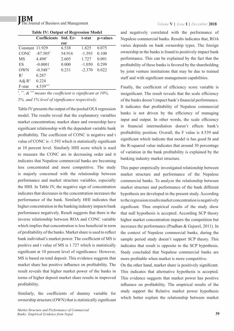
JBMVolume V | Issue I | December 2018The Journal of Business and Management
39
Table IV: Output of Regression ModelCoefficients Std. Er-
rort-stat p-values
Constant 11.929 6.538 1.825 0.075CONC -87.505* 54.916 -1.593 0.100MS 4.498* 2.605 1.727 0.091ES -0.0001 0.000 -1.050 0.299OWN -0.548** 0.231 -2.370 0.022R2 0.287Adj R2 0.224F-stat 4.539***
*, **, & *** means the coefficient is significant at 10%,5%, and 1% level of significance respectively.
Table IV presents the output of the pooled OLS regression model. The results reveal that the explanatory variables market concentration; market share and ownership have significant relationship with the dependent variable bank profitability. The coefficient of CONC is negative and t value of CONC is -1.593 which is statistically significant at 10 percent level. Similarly HHI score which is used to measure the CONC are in decreasing order and it indicates that Nepalese commercial banks are becoming less concentrated and more competitive. The study is majorly concerned with the relationship between performance and market structure variables, especially the HHI. In Table IV, the negative sign of concentration indicates that decreases in the concentration increases the performance of the bank. Similarly HHI indicates that higher concentration in the banking industry impacts bank performance negatively. Result suggests that there is the inverse relationship between ROA and CONC variable which implies that concentration is less beneficial in term of profitability of the banks. Market share is used to reflect bank individual’s market power. The coefficient of MS is positive and t value of MS is 1.727 which is statistically significant at 10 percent level of significance. However, MS is based on total deposit. This evidence suggests that market share has positive influence on profitability. The result reveals that higher market power of the banks in terms of higher deposit market share results in improved profitability.
Similarly, the coefficients of dummy variable for ownership structure (OWN) that is statistically significant
and negatively correlated with the performance of Nepalese commercial banks. Results indicates that, ROA varies depends on bank ownership types. The foreign ownership in the banks is found to positively impact bank performance. This can be explained by the fact that the profitability of these banks is favored by the shareholding by joint venture institutions that may be due to trained staff and with significant management capabilities.
Finally, the coefficient of efficiency score variable is insignificant. The result reveals that the scale efficiency of the banks doesn’t impact bank’s financial performance. It indicates that profitability of Nepalese commercial banks is not driven by the efficiency of managing input and output. In other words, the scale efficiency in financial intermediation doesn’t effects bank’s profitability position. Overall, the F value is 4.539 and significant which indicate that model is has good fit and the R-squared value indicates that around 30 percentage of variation in the bank profitability is explained by the banking industry market structure.
This paper empirically investigated relationship between market structure and performance of the Nepalese commercial banks. To analyze the relationship between market structure and performance of the bank different hypothesis are developed in the present study. According to the regression results market concentration is negatively significant. Thus empirical results of the study show that null hypothesis is accepted. According SCP theory higher market concentration impairs the competition but increases the performance (Pradhan & Gajurel, 2011). In the context of Nepalese commercial banks, during the sample period study doesn’t support SCP theory. This indicates that result is opposite to the SCP hypothesis. Study concluded that Nepalese commercial banks are more profitable when market is more competitive.On the other hand, market share is positively significant. This indicates that alternative hypothesis is accepted. This evidence suggests that market power has positive influence on profitability. The empirical results of the study support the Relative market power hypothesis which better explain the relationship between market
Market Structure and Performance of Commercial Banks: Empirical Evidence from Nepal
JBMVolume V | Issue I | December 2018The Journal of Business and Management
40
structure and performance of the bank in the context of Nepalese commercial banks. Therefore, larger Nepalese banks earn higher profits.
Similarly, the empirical result of the study showed that efficiency score is statistically insignificant. It means null hypothesis is accepted in the study. Evidence indicated that there is no relationship between the efficiency and performance in Nepalese commercial banks which is opposite to the efficiency structure theory. The result indicates that, more efficient banks are unable to make more profit. The reason behind this may be the shorter sample period and low number of sample of the study as well as selection of input and output for the study to assess the DEA efficiency score.
As far as ownership structure is concerned, alternative hypothesis is accepted in the study that stated profitability varies with ownership type. That depicts Joint venture banks are more profitable than local private banks. That may be caused due to the large market share held by the Joint venture banks in Nepal.
6. ConclusionThis study empirically investigated relationship between market structure and performance of the Nepalese commercial banks. Descriptive analysis of the study concluded that joint venture banks (JVC) are better in terms of profitability. In the same way JVC are able to occupy larger market share and seems more efficient. The study revealed that decrease in market concentration
increases the bank profitability in the context of Nepalese commercial banks. On the other hand, study results indicated that market power has positive influence on profitability. Therefore, larger Nepalese banks earn higher profits. On the contrary, empirical results indicated that there is no relationship between the bank’s efficiency and performance in Nepalese commercial banks. The result indicates that, more efficient banks are unable to make more profit. In the context of ownership structure of the bank, results indicate that, ROA differences depend on bank ownership types. Profitability of joint venture bank is larger than local private banks in Nepal.
The empirical results of this study have a number of policy and managerial applications. As the results of the study market concentration is negatively related with performance of the bank so that Policy makers should concentrate on policies that promotes market competition in banking industry and making less market concentration. Similarly Policy maker should focus on promoting foreign investment on banking industry as the study concluded that Profitability of joint venture bank is larger than local private banks in Nepal. Likewise study recommend for further study that can be conducted with larger sample size along with larger time period. Further research can conduct on longitudinal study (i.e before and after liberalization). Moreover researcher can conduct research using DEA efficiency score using intermediation approach and output orientation that may change the result.
Market Structure and Performance of Commercial Banks: Empirical Evidence from Nepal
ReferencesAyadi, I., & Ellouze, A. (2013). Market Structure and
Performance of Tunisian Banks. International Journal of Economics and Financial Issues , 3 (2), 345-354.
Bamakhramah, A. S. (1992). Measurement of Banking Structure in Saudi Arabia and Its Effect on Bank. J. KAU: Econ. & Adm. , 5, 3-29.
Bhatti, G. A., & Hussain, H. (2010). Evidence on Structure Conduct Performance Hypothesis In Pakistani. International Journal of Business and Management , 5 (9).
Claessens, S., Djankov, S., & Lang, L. (2000). The separation of ownership and control in East Asian corporations. Journal of Financial Economics, 58, 81–112.
Claeys, S., & Hainz, C. (2007). Acquisition versus greenfield: The impact of the mode of foreign bank entry on information and bank lending rates. International Review of Finance, 3, 105-29.
González, F. ( 2009). Determinants of Bank-Market

JBMVolume V | Issue I | December 2018The Journal of Business and Management
41
Structure: Efficiency and Political Economy Variables. Journal of money credit and banking , 41 (4), 735 - 754.
Kharel, R. S., & Pokhrel, D. R. (2012). Does Nepal’s
Financial Structure Matter for Economic Growth. NRB Economic Review .
Mensi, S., & Zouari, A. (2010). Efficient Structure versus Market Power: Theories and Empirical Evidence. International Journal of Economics and Finance , 2 (4).
O’Sullivan, J. A. (2012). Corporate governance, performance and risk-taking in the U. S. banking industry (Doctoral dissertations, University of New Orleans). Retrieved from ProQuest Dissertations and Theses Database. (UMI No. 3531151)
Pradhan, R. S., & Gajurel, D. P. (2011). Structure- Performance Relation in Nepalese Banking Industry. International Conference on Economics, Business , 2.
Tan, Y., & Floros, C. (2013). Market power, stability and performance in the Chinese banking industry. Economic Issues , 18 (2).
Thapa, M. (2010). Competitive Strategy and Performance of. PYC Nepal Journal of Management , 3 (1).
Ugwunta, D. O., Ani, W. U., Ugwuanyi, G. O., & Ugwu, J. N. (Eds.). (2012). Journal of Economics and Sustainable Development , 3 (7).
Zhengchao, L., & Qin, L. (Eds.). (2012). China Banking Market Structure and Performance: Based on Panel Data 2000-2010. International Business and Management , 5 (2).
Market Structure and Performance of Commercial Banks: Empirical Evidence from Nepal

JBMVolume V | Issue I | December 2018The Journal of Business and Management
42
Stock Price Behavior of Nepalese Commercial Banks: Random Walk Hypothesis
Nirajan Bam1, Rajesh Kumar Thagurathi2, Bipin Shrestha3
Abstract
Using the data set on daily stock prices during the fiscal year 2015/16 (Sept 23, 2015 through Dec 22, 2015), this paper attempts to analyze the random behavior of stock price of Nepalese Commercial Banks by using run test, serial correlation and run tests and martingale random walk hypothesis under heteroscedasticity assumption of standard error. The results conclude that the proposition of Random Walk Hypothesis (RWH) in Nepalese stock markets does not hold true. This conclusion corroborates with the conclusions of the past studies carried out in Nepalese context.
Key Words: Efficient Market, Nepal, Random Walk. Stock Price Behavior Theories
1. IntroductionFinancial sector has a crucial role to pool scattered savings for capital formation. Stock market in Nepalese financial market assists in mobilizing savings for economic sustainability. It allows the platform for the real sector growth which includes in the major infrastructural development of nation. But, the Nepalese securities market still is in growing stage. Its further development is crucial. In Nepal, the major constituent of the securities market is the shares of commercial banks and behavior of price of commercial banks influences the Nepal Stock Exchange index.
The studies on stock price behavior revealed a considerable interest in the long run time series properties of stock price, with a particular attention being paid to investigate whether stock prices characterized as random walk. If stock prices follow a mean reverting process then there exist a tendency for the price level to return to its trend path over time and investors may be able to forecast future returns by using information on its past returns. On the Contrary, a random walk process indicates that any shock to stock price is permanent and there is no tendency for the price level to return to a trend path over time.Normally, the stock market index is taken as a barometer of an economy. Growth in stock index is
normally considered as a good sign since it implies the investors are confident about the future prospect of the economy. It helps promote investment in the economy. However, a rapid increase in the stock market index is always a matter of concern. If the increase in the index is not justified by the fundamentals, such a rise cannot be sustained and eventually the index will plummet endangering the economic and financial stability.
Random walk hypothesis states that previous price changes or changes in return are useless in predicting future price or return changes. More precisely, this theory contends that successive price changes are independent and prices at any time, on the average, reflect the intrinsic value of security (Fischer & Jordan, 2000). Random walks in stock returns are important for the formulation of rational expectations models and the testing of weak-form market efficiency. Firstly, in an efficient market, prices of stocks fully incorporate all relevant information. Hence, stock returns will display unpredictable (or random walk) behavior. Secondly, the return generating process is dominated by a temporary component in stock prices those are not characterized by a random walk, and therefore, future returns can be predicted by the historical sequence of returns. Finally, the ability of stock markets to play the role that is usually ascribed to them - attracting foreign investment, boosting domestic saving
1 Lecturer, School of Business, Pokhara University, Nepal, 2 Associate Professor, School of Engineering, Pokhara University,3 Research Scholar, School of Business, Pokhara University, Nepal,
ISSN 2350-8868
JBMVolume V | Issue I | December 2018The Journal of Business and Management
43
and improving the pricing and availability of capital - depends upon the presence of random walks.
Efficient-market hypothesis (EMH) states that it is impossible to “beat the market” because stock market efficiency causes existing share prices to always incorporate and reflect all relevant information. According to the EMH, stocks always trade at their fair value on stock exchanges, making it impossible for investors to either purchase undervalued stocks or sell stocks for inflated prices.
The accelerating pace of development of capital market in Nepal has opened the avenues for utilization of funds for corporate sectors. It is well accepted fact that Nepal has abundant resources, both human and natural, to exploit, but at the same it is facing inadequacy of financial resources. As the resource mobilization domestically as well as internationally is crucial for Nepal to speed up its economic development, it is essential that the stock market be efficient.
Nepal stock market has not been researched on the basis of book value of the company. The objective of the paper is to identify the behavior of the Nepalese commercial banks. The study findings are expected to serve investors for gaining profit and enable the policy makers to improve the level of efficiency. The absence and presence of the random walk in the price generation in the stock market is evaluated by using stock market indices of eight banks (Four banks have market share price less than Rs.1000 and four banks have above RS. 1000) from 22-Dec-2015 to 22-Mar-2016.
2. Literature ReviewOyama (1997), Policy Development and Review Development Division has conducted a study entitled on “Determinants of Stock Prices: The Case of Zimbabwe”. The research study done by author focuses on the general relationship between stock prices and macroeconomics variables in Zimbabwe, using error-correction, model, the multi factor return – generating model. From the study author shows that despite the large fluctuation in stock prices since 1991, the analysis indicated that the
Zimbabwe Stock Exchange functioned quite consistently during that period.
Shubiri and Faris (2010) has conducted a study entitled on “Analysis of the Determinants of Market Stock Price Movements: An Empirical Study of Jordanian Commercial Banks”. In the study, simple and multiple regression analysis is conducted to find out the relationship microeconomic factors with the stock price and found highly positive significant relationship between market price of stock and net asset value per share; market price of stock dividend percentage, gross domestic product, and negative significant relationship on inflation and lending interest rate but not always significant on some years of Amman Stock Exchange in Jordan.
Shrestha, (2014) has conducted a study entitled on: “Determinants of Stock Market Performance in Nepal”. This research study empirically observes the determinants of the stock market performance in Nepal using monthly data for the period of mid-August 2000 to mid-July 2014. In the study, the impact of major changes in politics and Nepal Rastra Bank’s policy on lending against share collateral has also been assessed. Empirical results obtained from OLS estimations of behavioral equations disclosed that the performance of stock market is found to respond positively to inflation and broad money growth, and negatively to interest rate.
Islam et al. (2015) has conducted a study entitled on “Determinants of Stock Price Movements”: Evidence from Chittagong Stock Exchange, Bangladesh. The research focus on the incidents of 2010-2011 stock market crash in Bangladesh. The study aims to reexamine the relationship between stock price, dividend and retained earnings of 29 listed banks of Chittagong Stock Exchange, in the post-crash period. Cross-sectional data were collected from secondary sources. Using linear regression method, the study found that both, dividend and retained earnings of sample banks have strong influence over the stock price, though there was moderate explanatory power of those variables. This study concludes that both dividend and retained earnings are strong determinants of stock price at significant level.
Stock Price Behavior of Nepalese Commercial Banks: Random Walk Hypothesis
JBMVolume V | Issue I | December 2018The Journal of Business and Management
44
Baral et al. (2006) has conducted a study entitled on “Daily Stock Price Behavior of Commercial Banks in Nepal”. The study conducted by the authors focuses to analyze the stock price behavior of commercial banks in Nepalese markets. To conduct the study the technical analysis and fundamental analysis is used. The study done by authors reveals that the observations of daily stock prices of sampled banks indicate that there is a large variation in their stock prices in the fiscal year 2005/06 which shows that banks are not doing well in Nepalese stock market. Also looking on the serial coefficients it can be stated that the values are significantly deviated from zero and statistically insignificant. It signifies that the successive price changes are dependent.
Pradhan et al. (2010) has conducted a study entitled on “Efficient market hypothesis and behavior of Share prices: the Nepalese evidence”. The study conducted by authors’ aims to assess equity share price behavior in Nepal and testing the hypothesis that share price changes are independent. In viewing the Auto-correlation test it shows that the random walk hypothesis is true for less frequently traded stocks and the same was not consistent with the prices of highly traded stocks. The study result also indicate that the random walk hypothesis is true for less frequently traded stocks and the same is not consistent with the prices of highly traded stocks.
Dangol (2010) has conducted a study entitled on “Testing Random-Walk Behavior in Nepalese Stock Market”. The study conducted by author aim to measure the behavior of the stock returns in the Nepal Stock Exchange (NEPSE) using Augmented Dickey-Fuller (ADF) and Phillips-Perron (PP) unit root tests. The study of the author reveals that the random walk hypothesis for NEPSE index is rejected during the period of analysis. The Nepalese stock market is inefficient in daily returns series suggesting that past movements in stock prices can be used to predict their future movements.
3. Data and Methodology3.1 DataThere are 231 companies which are listed in NEPSE as on 30th March 2016. The sample firms among the listed
companies selected for the study are A-class financial institutions. In this study, commercial bank represent the population and the number of the banks is 31 during the study period. Stratified sampling technique is used in which population is divided into homogenous groups (strata). Simply strata are designed on the basis of market price of share as: (i) MPS above Rs.1000 and
(ii) MPS below Rs.1000 and among them 8 commercial banks have been selected as a sample employing purposive sampling technique. The sample banks are as follows:
� MPS above Rs.1000• Everest Bank Limited• Nabil Bank Limited• Nepal SBI Bank Limited• Standard Chartered Bank Nepal Limited
� MPS below Rs.1000• Kumari Bank Limited• Laxmi Bank Limited• Bank of Kathmandu• Siddhartha Bank Limited
Closing daily share prices of above mentioned commercial banks during the study period covering three months from 23-Sep-2015 to 22-Dec-2015 are used as observations for the study.
3.2 Research MethodsMany statistical test are performed by the past research scholars to identify the random walk behavior of the stock price however following test are performed in this research.
Runs TestRuns test is a non-parametric test that ignores the magnitude of price changes and observes only direction of changes in a given time series. For the present purpose, a run can be defined as a sequence of price changes of the same sign preceded and followed by price changes of different sign. For stock prices, there are three different possible types of price changes in a series, i.e., positive, negative and no-change, and thus three different types of runs. One sample runs test is a test used to judge the
Stock Price Behavior of Nepalese Commercial Banks: Random Walk Hypothesis

JBMVolume V | Issue I | December 2018The Journal of Business and Management
45
randomness of a sample on the basic of the order in which the observations are taken. The sampling distribution of ‘r’ statistic, the number of runs is to be used and this distribution has its mean and the standard deviation. Here the mean and standard error associated with the sampling distribution of r which can be expressed as:
μ r = (2n1*n2/n1+n2) +1
z = r- μ r / σrσr = √
________________________________
2n1
*n2 (2n1*n2-n1-n2) / (n1+n2)
2 (n1+n2-1) ............... (1)
Upper Limit: μ r + z σr ,Lower Limit: μ r - z σr
Autocorrelation TestIt is now a common practice to treat the terms serial correlation and auto correlation synonymously (Gujarati, 2004). Serial correlation and auto correlation are considered synonymous. The autocorrelation coefficient (ρk) provides a measure of the relationship between the value of a random variable in time‘t’ and its value ‘k’ periods earlier. In other words, it will indicate whether price changes at time‘t’ is influenced by the price changes occurring ‘k’ period earlier. A significant positive autocorrelation indicates the presence of trends. The presence of negative autocorrelation documents the existence of more reversals that might occur randomly. Numbers that are truly random will have zero serial correlation. For example, for the variable μt , defined as the change in log price of a given security from the end of the day ‘t-1’ to the end of the day ‘t’, the autocorrelation coefficient for lag ‘k’ is:
rk = Cov(mt, mt·1 ) Var(mt )
.................... (2)
Box- Ljung testLjung and Box (1978) develop the Box-Ljung test to examine the lack of fit of time series data, which define:Ho: Model doesn’t exhibit lack of fitH1: Model exhibit the lack of fitTest statistics is defined as
.......................(3)
Where rˆ2 k estimated autocorrelation of the series at lag k and m is the number of lags being tested
Martingale Random Walk HypothesisAccording to Arlt and Arltová (2000), martingale model belongs to the earliest models of the financial asset prices. Its origin lies in the birth of the probability theory and the historic of game of chance. It follows a principle of a fair game i.e. the game neither in your favor nor your pennant’s. Martingale is a stochastic process {Pt} which satisfied following condition:E [Pt/Pt-1,Pt-2,…] = Pt ............................(3)Equivalently, it is possible to writeE [Pt - Pt-1/Pt-1, Pt-2, …] = 0......................(4)If Pt is the asset’s price at time t, the martingale hypothesis means that tomorrow’s price is expected to be equal to today’s price under the condition of the entire history development of the asset’s price. The forecasting meaning follows: the martingale hypothesis implies that the “best” forecast (from the point of view of mean square error) of tomorrow’s price is simply today’s price.
Historically, the martingale is closely related to hypothesis of efficient market which means that the information contained in past asset’s prices is completely reflected in the current price. In efficient market it is not possible to profit by trading on the information contained in the asset’s price history. Despite the fact that the modern financial economics considers the necessity of some trade-off between risk and expected returns, martingale is still powerful tool and has important applications in theory of asset prices. Another aspect of martingale is that it is basis for the development of a closely related model which is called random walk.
Lo and Mickinly (1988) develop the special approach of variance ratio test for the null hypothesis of a martingale, which is robust to heteroskedastic standard errors.The time series follows a random walk then the variance should be proportional of the some interval, i.e
....................(6)
The statistical test is given as
...................(7)
Stock Price Behavior of Nepalese Commercial Banks: Random Walk Hypothesis
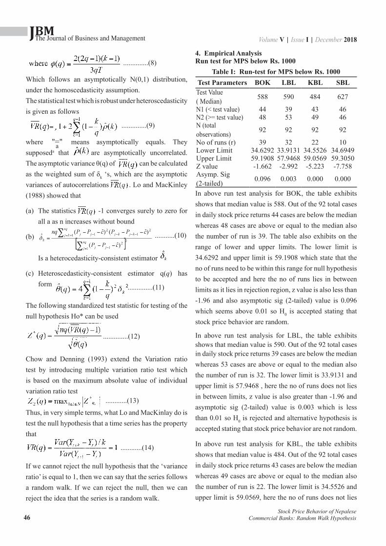
JBMVolume V | Issue I | December 2018The Journal of Business and Management
46
..............(8)
Which follows an asymptotically N(0,1) distribution, under the homoscedasticity assumption.The statistical test which is robust under heteroscedasticity is given as follows
..............(9)
where "="a means asymptotically equals. They supposeda that are asymptotically uncorrelated. The asymptotic variance θ(q) of can be calculated as the weighted sum of δk ‘s, which are the asymptotic variances of autocorrelations . Lo and MacKinley (1988) showed that
(a) The statistics -1 converges surely to zero for all a as n increases without bound
(b) ...........(10)
Is a heterocedasticity-consistent estimator kδ
(c) Heteroscedasticity-consistent estimator q(q) has form ..............(11)
The following standardized test statistic for testing of the null hypothesis Ho* can be used
..............(12)
Chow and Denning (1993) extend the Variation ratio test by introducing multiple variation ratio test which is based on the maximum absolute value of individual variation ratio test
............(13)
Thus, in very simple terms, what Lo and MacKinlay do is test the null hypothesis that a time series has the property that
............(14)
If we cannot reject the null hypothesis that the ‘variance ratio’ is equal to 1, then we can say that the series follows a random walk. If we can reject the null, then we can reject the idea that the series is a random walk.
4. Empirical AnalysisRun test for MPS below Rs. 1000
Table I: Run-test for MPS below Rs. 1000Test Parameters BOK LBL KBL SBLTest Value ( Median) 588 590 484 627
N1 (< test value) 44 39 43 46N2 (>= test value) 48 53 49 46N (total observations) 92 92 92 92
No of runs (r) 39 32 22 10Lower Limit 34.6292 33.9131 34.5526 34.6949Upper Limit 59.1908 57.9468 59.0569 59.3050Z value -1.662 -2.992 -5.223 -7.758Asymp. Sig (2-tailed) 0.096 0.003 0.000 0.000
In above run test analysis for BOK, the table exhibits shows that median value is 588. Out of the 92 total cases in daily stock price returns 44 cases are below the median whereas 48 cases are above or equal to the median also the number of run is 39. The table also exhibits on the range of lower and upper limits. The lower limit is 34.6292 and upper limit is 59.1908 which state that the no of runs need to be within this range for null hypothesis to be accepted and here the no of runs lies in between limits as it lies in rejection region, z value is also less than -1.96 and also asymptotic sig (2-tailed) value is 0.096 which seems above 0.01 so H0 is accepted stating that stock price behavior are random.
In above run test analysis for LBL, the table exhibits shows that median value is 590. Out of the 92 total cases in daily stock price returns 39 cases are below the median whereas 53 cases are above or equal to the median also the number of run is 32. The lower limit is 33.9131 and upper limit is 57.9468 , here the no of runs does not lies in between limits, z value is also greater than -1.96 and asymptotic sig (2-tailed) value is 0.003 which is less than 0.01 so H0 is rejected and alternative hypothesis is accepted stating that stock price behavior are not random.
In above run test analysis for KBL, the table exhibits shows that median value is 484. Out of the 92 total cases in daily stock price returns 43 cases are below the median whereas 49 cases are above or equal to the median also the number of run is 22. The lower limit is 34.5526 and upper limit is 59.0569, here the no of runs does not lies
Stock Price Behavior of Nepalese Commercial Banks: Random Walk Hypothesis
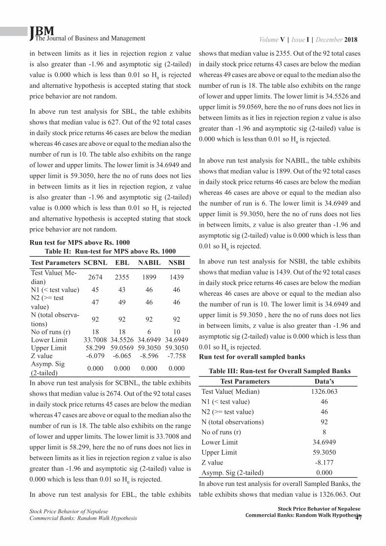
JBMVolume V | Issue I | December 2018The Journal of Business and Management
47
in between limits as it lies in rejection region z value is also greater than -1.96 and asymptotic sig (2-tailed) value is 0.000 which is less than 0.01 so H0 is rejected and alternative hypothesis is accepted stating that stock price behavior are not random.
In above run test analysis for SBL, the table exhibits shows that median value is 627. Out of the 92 total cases in daily stock price returns 46 cases are below the median whereas 46 cases are above or equal to the median also the number of run is 10. The table also exhibits on the range of lower and upper limits. The lower limit is 34.6949 and upper limit is 59.3050, here the no of runs does not lies in between limits as it lies in rejection region, z value is also greater than -1.96 and asymptotic sig (2-tailed) value is 0.000 which is less than 0.01 so H0 is rejected and alternative hypothesis is accepted stating that stock price behavior are not random.
Run test for MPS above Rs. 1000Table II: Run-test for MPS above Rs. 1000
Test Parameters SCBNL EBL NABIL NSBITest Value( Me-dian) 2674 2355 1899 1439
N1 (< test value) 45 43 46 46N2 (>= test value) 47 49 46 46
N (total observa-tions) 92 92 92 92
No of runs (r) 18 18 6 10Lower Limit 33.7008 34.5526 34.6949 34.6949Upper Limit 58.299 59.0569 59.3050 59.3050Z value -6.079 -6.065 -8.596 -7.758Asymp. Sig (2-tailed) 0.000 0.000 0.000 0.000
In above run test analysis for SCBNL, the table exhibits shows that median value is 2674. Out of the 92 total cases in daily stock price returns 45 cases are below the median whereas 47 cases are above or equal to the median also the number of run is 18. The table also exhibits on the range of lower and upper limits. The lower limit is 33.7008 and upper limit is 58.299, here the no of runs does not lies in between limits as it lies in rejection region z value is also greater than -1.96 and asymptotic sig (2-tailed) value is 0.000 which is less than 0.01 so H0 is rejected.
In above run test analysis for EBL, the table exhibits
shows that median value is 2355. Out of the 92 total cases in daily stock price returns 43 cases are below the median whereas 49 cases are above or equal to the median also the number of run is 18. The table also exhibits on the range of lower and upper limits. The lower limit is 34.5526 and upper limit is 59.0569, here the no of runs does not lies in between limits as it lies in rejection region z value is also greater than -1.96 and asymptotic sig (2-tailed) value is 0.000 which is less than 0.01 so H0 is rejected.
In above run test analysis for NABIL, the table exhibits shows that median value is 1899. Out of the 92 total cases in daily stock price returns 46 cases are below the median whereas 46 cases are above or equal to the median also the number of run is 6. The lower limit is 34.6949 and upper limit is 59.3050, here the no of runs does not lies in between limits, z value is also greater than -1.96 and asymptotic sig (2-tailed) value is 0.000 which is less than 0.01 so H0 is rejected.
In above run test analysis for NSBI, the table exhibits shows that median value is 1439. Out of the 92 total cases in daily stock price returns 46 cases are below the median whereas 46 cases are above or equal to the median also the number of run is 10. The lower limit is 34.6949 and upper limit is 59.3050 , here the no of runs does not lies in between limits, z value is also greater than -1.96 and asymptotic sig (2-tailed) value is 0.000 which is less than 0.01 so H0 is rejected.Run test for overall sampled banks
Table III: Run-test for Overall Sampled BanksTest Parameters Data’s
Test Value( Median) 1326.063N1 (< test value) 46N2 (>= test value) 46N (total observations) 92No of runs (r) 8Lower Limit 34.6949Upper Limit 59.3050Z value -8.177Asymp. Sig (2-tailed) 0.000
In above run test analysis for overall Sampled Banks, the table exhibits shows that median value is 1326.063. Out
Stock Price Behavior of Nepalese Commercial Banks: Random Walk Hypothesis
Stock Price Behavior of Nepalese Commercial Banks: Random Walk Hypothesis
JBMVolume V | Issue I | December 2018The Journal of Business and Management
48
of the 92 total cases in daily stock price returns 46 cases are below the median whereas 46 cases are above or equal to the median also the number of run is 8. The table also exhibits on the range of lower and upper limits. The lower limit is 34.6949 and upper limit is 59.3050, here the no of runs does not lies in between limits as it lies in rejection region, z value is also greater than -1.96 and asymptotic sig (2-tailed) value is 0.000 which is less than 0.01 so H0 is rejected stating that stock price behavior are not random.
Serial Correlation Analysis
Serial Correlation MPS below Rs. 1000In serial correlation, different data’s were exhibited as ACF (autocorrelation function), auto-correlation coefficient, standard error, box L-jung statistics and significance level of each of the banks having MPS < Rs1000 were presented. While analysis 16 lags period is observed. The auto-correlation coefficient includes both positive and negative valued data. Since all significance values in box L-jung statistics are below 0.05 level of significance so this results shows that stock price of banks having MPS below Rs.1000 are of non-random nature.
Serial Correlation for MPS above Rs. 1000In serial correlation, different data’s were exhibited as ACF (autocorrelation function), auto-correlation coefficient, standard error, box L-jung statistics and significance level of each of the banks having MPS > Rs1000 were presented. While analysis 16 lags period is observed. The auto-correlation coefficient includes both positive and negative valued data. Since all significance values in box L-jung statistics are below 0.05 level of significance so this results shows that stock price of banks having MPS above Rs.1000 are of non-random nature. The results are shown in Appendix II.
Serial Correlation for Overall Sampled BanksIn serial correlation, different data’s were exhibited as ACF (autocorrelation function), auto-correlation coefficient, standard error, box L-jung statistics and significance level of each of the sampled banks were presented. While analysis 16 lags period is observed. The auto-correlation coefficient includes both positive and negative valued data. Since all significance values in box L-jung statistics fall below 5% level of significance so that stock price of overall sampled banks in aggregate are of non-random nature.
Martingale Variance Ratio TestTable IV : Martingale Variance Ratio Test of Bank having Book Value Rs.(< 1000)
H0 : First Lag of Laxmi Bank is Martingale Ho : First Lag of Bank of Kathmandu is MartingaleHeteroskedasticity robust standard error estimates Heteroskedasticity robust standard error estimatesJoint Tests Value df Probability Joint Tests Value df ProbabilityMax |z| (at period 2)* 3.388468 90 0.0028 Max |z| (at period 4)* 2.778093 91 0.0217
Individual Tests Individual TestsPeriod Var. Ratio Std. Error z-Statistic Probability Period Var. RatioStd. Errorz-StatisticProbability
2 0.442482 0.164534 -3.38847 0.0007 2 0.765324 0.128664 -1.82395 0.06824 0.279876 0.265641 -2.71089 0.0067 4 0.39081 0.219283 -2.77809 0.00558 0.133181 0.377002 -2.29924 0.0215 8 0.237927 0.321737 -2.36862 0.017916 0.060302 0.516398 -1.81972 0.0688 16 0.123951 0.446628 -1.96148 0.0498
Ho : First Lag of Kumari Bank is Random Ho: First Lag of KUMARI Bank is a martingaleStandard error estimates assume no heteroskedasticity Heteroskedasticity robust standard error estimatesJoint Tests Value df Probability Joint Tests Value df ProbabilityMax |z| (at period 2)* 5.341164 90 0 Max |z| (at period 2)* 1.948862 90 0.19Wald (Chi-Square) 28.94446 4 0 Individual TestsIndividual Tests Period Var. RatioStd. Errorz-StatisticProbability
Period Var. Ratio Std. Error z-Statistic Probability 2 0.436992 0.288891 -1.94886 0.05132 0.436992 0.105409 -5.34116 0 4 0.229845 0.452099 -1.70351 0.08854 0.229845 0.197203 -3.9054 0.0001 8 0.135924 0.570213 -1.51536 0.12978 0.135924 0.311805 -2.77121 0.0056 16 0.060214 0.668967 -1.40483 0.1601
16 0.060214 0.46398 -2.02549 0.0428
Stock Price Behavior of Nepalese Commercial Banks: Random Walk Hypothesis
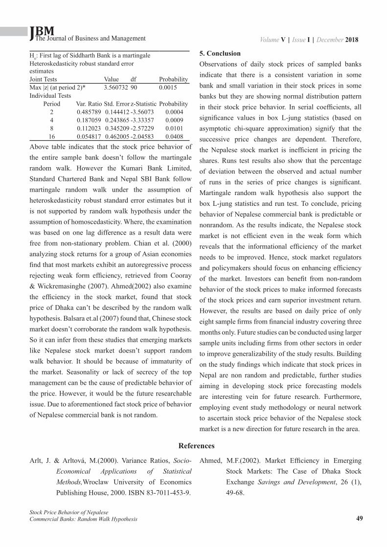
JBMVolume V | Issue I | December 2018The Journal of Business and Management
49Stock Price Behavior of Nepalese Commercial Banks: Random Walk Hypothesis
Ho: First lag of Siddharth Bank is a martingaleHeteroskedasticity robust standard error estimatesJoint Tests Value df ProbabilityMax |z| (at period 2)* 3.560732 90 0.0015Individual Tests
Period Var. Ratio Std. Error z-Statistic Probability2 0.485789 0.144412 -3.56073 0.00044 0.187059 0.243865 -3.33357 0.00098 0.112023 0.345209 -2.57229 0.010116 0.054817 0.462005 -2.04583 0.0408
Above table indicates that the stock price behavior of the entire sample bank doesn’t follow the martingale random walk. However the Kumari Bank Limited, Standard Chartered Bank and Nepal SBI Bank follow martingale random walk under the assumption of heteroskedasticity robust standard error estimates but it is not supported by random walk hypothesis under the assumption of homoscedasticity. Where, the examination was based on one lag difference as a result data were free from non-stationary problem. Chian et al. (2000) analyzing stock returns for a group of Asian economies find that most markets exhibit an autoregressive process rejecting weak form efficiency, retrieved from Cooray & Wickremasinghe (2007). Ahmed(2002) also examine the efficiency in the stock market, found that stock price of Dhaka can’t be described by the random walk hypothesis. Balsara et.al (2007) found that, Chinese stock market doesn’t corroborate the random walk hypothesis. So it can infer from these studies that emerging markets like Nepalese stock market doesn’t support random walk behavior. It should be because of immaturity of the market. Seasonality or lack of secrecy of the top management can be the cause of predictable behavior of the price. However, it would be the future researchable issue. Due to aforementioned fact stock price of behavior of Nepalese commercial bank is not random.
5. ConclusionObservations of daily stock prices of sampled banks indicate that there is a consistent variation in some bank and small variation in their stock prices in some banks but they are showing normal distribution pattern in their stock price behavior. In serial coefficients, all significance values in box L-jung statistics (based on asymptotic chi-square approximation) signify that the successive price changes are dependent. Therefore, the Nepalese stock market is inefficient in pricing the shares. Runs test results also show that the percentage of deviation between the observed and actual number of runs in the series of price changes is significant. Martingale random walk hypothesis also support the box L-jung statistics and run test. To conclude, pricing behavior of Nepalese commercial bank is predictable or nonrandom. As the results indicate, the Nepalese stock market is not efficient even in the weak form which reveals that the informational efficiency of the market needs to be improved. Hence, stock market regulators and policymakers should focus on enhancing efficiency of the market. Investors can benefit from non-random behavior of the stock prices to make informed forecasts of the stock prices and earn superior investment return. However, the results are based on daily price of only eight sample firms from financial industry covering three months only. Future studies can be conducted using larger sample units including firms from other sectors in order to improve generalizability of the study results. Building on the study findings which indicate that stock prices in Nepal are non random and predictable, further studies aiming in developing stock price forecasting models are interesting vein for future research. Furthermore, employing event study methodology or neural network to ascertain stock price behavior of the Nepalese stock market is a new direction for future research in the area.
References
Arlt, J. & Arltová, M.(2000). Variance Ratios, Socio-Economical Applications of Statistical Methods,Wroclaw University of Economics Publishing House, 2000. ISBN 83-7011-453-9.
Ahmed, M.F.(2002). Market Efficiency in Emerging Stock Markets: The Case of Dhaka Stock Exchange Savings and Development, 26 (1), 49-68.

JBMVolume V | Issue I | December 2018The Journal of Business and Management
50
Balsara, N.J., Chen G., & Zheng L.(2007). The Chinese Stock Market: An Examination of the Random Walk Model and Technical Trading Rules. Quarterly Journal of Business and Economics, Vol. 46(2), 43-63.
Baral,K.J.& Shrestha, S.K.(2006) Daily Stock Price Behavior of Commercial Banks Banks in Nepal. The Journal of Nepalese Business Studies, 1, 1-11.
Chiang T. C, Yang, S. Y. & Wang T. S. (2000). Stock Return and Exchange Rate Risk: Evidence from Asian Stock Markets Based on a Bivariate GARCH Model. International Journal of Business 2, 97-1
Chow, K.V. & Denning. K.C. (1993). A simple multiple variance ratio test. Journal of Econometrics ,58, 385-401.
Cooray, A & Wickremasinghe, G.(2007). The Efficiency of Emerging Stock Markets: Empirical Evidence from the South Asian Region. The Journal of Developing Areas, 41, (1), 171-183.
Dangol, J (2010) “Testing Random-Walk Behavior in Nepalese Stock Market”. PYC Nepal Journal of Management, 1, 28-36
Horne, V & Wachowicz,(2000), “Investments. New Delhi: Prentice Hall of India Pvt. Ltd
Islam, Syedul.M. & Dooty. Nusrat, E.( 2015) .Determinants of Stock Price Movements: Evidence from Chittagong Stock Exchange, Bangladesh. Journal of Economics and Business Research, 2, 117-133.
Ljung G & Box G (1978) . On a Measure of Lack of Fit in
Time Series Models, Biometrika, 65, 297-303
Oyama, T (1997). Determinants of Stock Prices: The Case of Zimbabwe.
Pradhan, R.S. & Saraswati, KC (2010) Efficient market hypothesis and behavior of Share prices:the Nepalese evidence, SEBO Journal Vol. IV,104-117
Shrestha,K. P & Subedi, B.R. (2014) Determinants of Stock Market Performance in Nepal. NRB Economic Review, 25-40.
Shrestha,K. P & Subedi, B.R. (2014) Determinants of Stock Market Performance in Nepal. NRB Economic Review, 25-40.
Shubiri, Faris N.(2010).Analysis the Determinants of Market Stock Price Movements: An Empirical Study of Jordanian Commercial Banks. International Journal of Business and Management , 5(10),1-11.
Walter, J. E. (1963) . Dividend Policy: Its influence on the Value of Enterprise, Journal of Finance, XXXI, 280-291.
Weston, J.F. & Brigham, E. F. ( 1 9 8 7 ) . Essentials of Managerial Finance. Chicago: The Dryden Press.
Weston, B. and Brigham, E. F (1995). Essentials of Managerial Finance. New Delhi: Prentice Hall of India Pvt. Ltd.
Zahir, K & Shah, M. (1982). Issues of Book Value Per Share and its Impacts on BFI’s .Journal of Finance, XXXI, 280-291.
Stock Price Behavior of Nepalese Commercial Banks: Random Walk Hypothesis
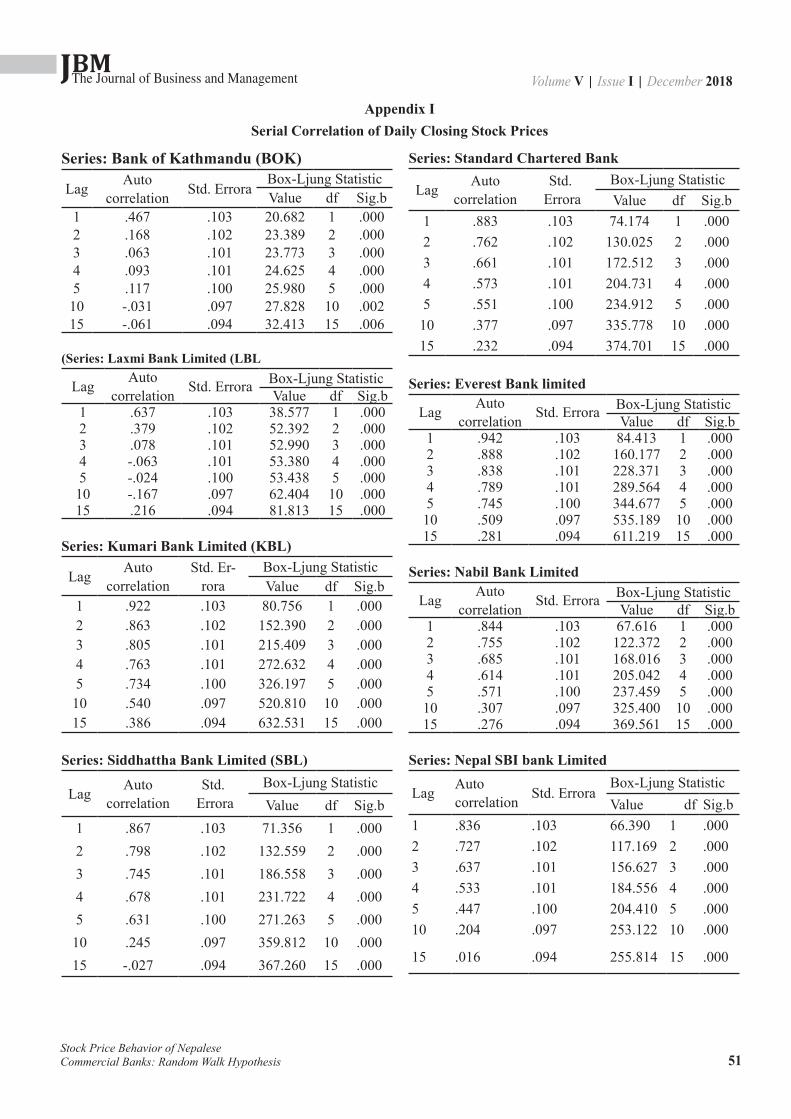
JBMVolume V | Issue I | December 2018The Journal of Business and Management
51Stock Price Behavior of Nepalese Commercial Banks: Random Walk Hypothesis
Series: Bank of Kathmandu (BOK)
Lag Auto correlation Std. Errora
Box-Ljung StatisticValue df Sig.b
1 .467 .103 20.682 1 .0002 .168 .102 23.389 2 .0003 .063 .101 23.773 3 .0004 .093 .101 24.625 4 .0005 .117 .100 25.980 5 .00010 -.031 .097 27.828 10 .00215 -.061 .094 32.413 15 .006
(Series: Laxmi Bank Limited (LBL
Lag Autocorrelation Std. Errora Box-Ljung Statistic
Value df Sig.b1 .637 .103 38.577 1 .0002 .379 .102 52.392 2 .0003 .078 .101 52.990 3 .0004 -.063 .101 53.380 4 .0005 -.024 .100 53.438 5 .00010 -.167 .097 62.404 10 .00015 .216 .094 81.813 15 .000
Series: Kumari Bank Limited (KBL)
Lag Autocorrelation
Std. Er-rora
Box-Ljung StatisticValue df Sig.b
1 .922 .103 80.756 1 .0002 .863 .102 152.390 2 .0003 .805 .101 215.409 3 .0004 .763 .101 272.632 4 .0005 .734 .100 326.197 5 .00010 .540 .097 520.810 10 .00015 .386 .094 632.531 15 .000
Series: Siddhattha Bank Limited (SBL)
Lag Autocorrelation
Std. Errora
Box-Ljung StatisticValue df Sig.b
1 .867 .103 71.356 1 .0002 .798 .102 132.559 2 .0003 .745 .101 186.558 3 .0004 .678 .101 231.722 4 .0005 .631 .100 271.263 5 .00010 .245 .097 359.812 10 .00015 -.027 .094 367.260 15 .000
Series: Standard Chartered Bank
Lag Autocorrelation
Std. Errora
Box-Ljung StatisticValue df Sig.b
1 .883 .103 74.174 1 .0002 .762 .102 130.025 2 .0003 .661 .101 172.512 3 .0004 .573 .101 204.731 4 .0005 .551 .100 234.912 5 .00010 .377 .097 335.778 10 .00015 .232 .094 374.701 15 .000
Series: Everest Bank limited
Lag Autocorrelation Std. Errora Box-Ljung Statistic
Value df Sig.b1 .942 .103 84.413 1 .0002 .888 .102 160.177 2 .0003 .838 .101 228.371 3 .0004 .789 .101 289.564 4 .0005 .745 .100 344.677 5 .00010 .509 .097 535.189 10 .00015 .281 .094 611.219 15 .000
Series: Nabil Bank Limited
Lag Auto correlation Std. Errora Box-Ljung Statistic
Value df Sig.b1 .844 .103 67.616 1 .0002 .755 .102 122.372 2 .0003 .685 .101 168.016 3 .0004 .614 .101 205.042 4 .0005 .571 .100 237.459 5 .00010 .307 .097 325.400 10 .00015 .276 .094 369.561 15 .000
Series: Nepal SBI bank Limited
Lag Autocorrelation Std. Errora
Box-Ljung StatisticValue df Sig.b
1 .836 .103 66.390 1 .0002 .727 .102 117.169 2 .0003 .637 .101 156.627 3 .0004 .533 .101 184.556 4 .0005 .447 .100 204.410 5 .00010 .204 .097 253.122 10 .000
15 .016 .094 255.814 15 .000
Appendix ISerial Correlation of Daily Closing Stock Prices

JBMVolume V | Issue I | December 2018The Journal of Business and Management
52
Series: Average Value
Lag Autocorrelation Std. Errora Box-Ljung Statistic
Value df Sig.b1 .896 .103 76.246 1 .0002 .790 .102 136.182 2 .0003 .690 .101 182.402 3 .0004 .595 .101 217.228 4 .0005 .541 .100 246.282 5 .00010 .357 .097 332.815 10 .00015 .299 .094 386.372 15 .000
Appendix IIMartingale variance ratio test of bank having book value RS.(>1000)
Stock Price Behavior of Nepalese Commercial Banks: Random Walk Hypothesis
H0 : First Lag of Everst Bank is a Martingale Ho : First Lag of Nabil Bank is a MartingaleHeteroskedasticity robust standard error estimates Heteroskedasticity robust standard error estimatesJoint Tests Value df Probability Joint Tests Value df ProbabilityMax |z| (at period 4) 3.145477 90 0.0066 Max |z| (at period 4)* 2.778093 90 0.0217
Individual Tests Individual TestsPeriod Var. Ratio Std. Error z-Statistic Probability Period Var. Ratio Std. Error z-Statistic Probability
2 0.583055 0.150472 -2.77091 0.0056 2 0.45148 0.171538 -3.197767 0.00144 0.209932 0.251176 -3.14548 0.0017 4 0.229646 0.279983 -2.75143 0.00598 0.136045 0.352321 -2.45218 0.0142 8 0.109286 0.373877 -2.38237 0.017216 0.084862 0.483982 -1.89085 0.0586 16 0.071315 0.492117 -1.88712 0.0591
Null Hypothesis: Log of SBI Bank is a Martingale Heteroskedasticity robust standard error estimates
Null Hypothesis: DSBI is a Random WalkStandard error estimates assume ni heteroskedasticit
Joint Tests Value df Probability Joint Tests Value df Probability
Max |z| (at period 2) 1.915913 90 0.02032*** Max |z| (at period 2)* 4.81566 90 0
Individual TestsWald (Chi-square) 23.21851 4 0.0001
Individual TestsPeriod Var. Ratio Std. Error z-Statistic Probability Period Var. Ratio Std. Error z-Statistic Probability
2 0.492385 0.264947 -1.91591 0.0554 2 0.492385 0.105409 -4.81566 04 0.255857 0.41344 -1.79988 0.0719 4 0.255857 0.197203 -3.77349 0.00028 0.138274 0.51187 -1.68349 0.0923 8 0.138274 0.311805 -2.76367 0.005716 0.062445 0.582854 -1.60856 0.1077 16 0.062445 0.46398 -2.02068 0.0433
H0 : Lag of Stancdard Chartered Banks is a Martingale Ho : First Lag of Standard Chartered Bank is RandomHeteroskedasticity robust standard error estimates Stnadard error estimates assume in heteroskedasticitJoint Tests Value df Probability Joint Tests Value df ProbabilityMax |z| (at period 4) 2.09914 90 0.137*** Max |z| (at period 4)* 3.573821 90 0.0014
Individual TestsWald (Chi-square) 23.21851 4 0.0086Individual Tests
Period Var. Ratio Std. Error z-Statistic Probability Period Var. Ratio Std. Error z-Statistic Probability
24816
0.6429310.2952330.1323250.073862
0.21650.3357410.4203220.503956
-1.64928-2.09914-2.06431-1.83774
0.09910.03580.0390.0661
24816
0.6429310.2952330.1323250.073862
0.1054090.1972030.3118050.46398
-3.38745-3.57382-2.78275-1.99507
0.00070.00040.00540.0459

JBMVolume V | Issue I | December 2018The Journal of Business and Management
53
Socio-Cultural, Economic and Environmental Impact of Tibetan Refugee Settlement on Host
Community in PokharaSantosh Kumar Gurung1 , Bal Ram Bhattarai2, Shanti Devi Chhetri3, Anisha Bataju 4, Ganga Ghale5
Abstract
The study attempts to empirically investigate and assess the socio-cultural, economic and environmental impact of the refugee settlements on the local host community who are living around the Tashi Pakhiel Tibetan camp located in Hemja, Kaski district. A questionnaire survey was undertaken to collect opinion of 500 host community members on the issue. The findings reveal that there exists social harmony, mutual co-existence, and bonding between the Tibetan refugees and local residents of Hemja. The two communities involve in social exchange and participate in social events of each other. The social acceptance is revealed from the fact that the practice of intermarriages between the communities is also prevalent. The Tibetan refugee camp is found not to adversely impact the host community culture. Similarly, the refugee settlement has not brought any adverse effect on the local environment. The basic services and facilities like education and health is available on equitable basis to both the communities. Finally, the economic interaction between the communities has resulted in mutually beneficial economic condition for both in terms of increased business and employment opportunities. Moreover, the economic benefits to the host community are found to be relatively higher as compared to the benefits received by the refugees.
Keywords: Environmental Impact, Tibetan refugees, Socio-cultural, Economic
1. Lecturer, School of Business, Pokhara University2. Associate Professor, School of Business, Pokhara University3. Lecturer, School of Business, Pokhara University4. Research Scholar, School of Business, Pokhara University5. Research Scholar, School of Business, Pokhara University
1. IntroductionThe refugee issue is as complex as its causes, solutions and effects. Obviously, it is a clear humanitarian, moral and development issue facing humanity. Millions of people get displaced globally as a result of conflict, violence, and human rights violations. It is generally recognized that there are humanitarian, political, security, and development challenges during the time of displacement and the period after durable solutions have been identified, either in the home country, a neighboring state, or elsewhere. The world refugee problem is caused by a variety of reasons; factors and forces.
The responses of host countries to these mass influxes have varied greatly, both between states and, for single governments, over time and by refugee group. Some governments have received refugees with generosity, providing them with assistance and guaranteeing their
safety. Others have tried to prevent refugees from entering or have treated them harshly, restricting their movements and even endangering their safety (Jacobsen 1996, Aristide 1992). The majority of countries hosting large numbers of refugees are developing and poor countries. Developing countries that host refugees for protracted periods can experience long-term, economic, social and environmental consequences (UNHCR Standing Committee, 1997). Nepal is also not an exception of the refugee problem. Specifically, Nepal has faced problems associated with Tibetans and Bhutanese refugees.
An official record of the Government of Nepal confirms that 12,540 Tibetans living in different parts of Nepal, however the actual number of Tibetan refugees in Nepal at present is estimated to be around 20,000 as the government has not updated the record since 1993. The Tibetan refugees living in Nepal are dispersed in over
ISSN 2350-8868
JBMVolume V | Issue I | December 2018The Journal of Business and Management
54
21 districts of the country in Tibetan refugee camps (NUCRA, 2010). In 1960, upon the request of Nepalese authority, the International Committee of the Red Cross (ICRC) established emergency relief camps. In a similar vein, the Nepalese government, with the assistance of funds donated by the office of the United Nations High Commissioner for Refugee (UNHCR) also set up refugee shelter homes. Till the mid-1980s, the Nepalese government welcomed the Tibetan Refugees with open hands as the latter were not perceived as a threat to Nepalese diplomatic relations with China (IRIN, 2013).
The impact of refugees on host communities has largely been assumed to be negative. On the other hand some also believe that the influx of the refugees create a new context in which hosts devised strategies to gain access to incoming resources and to maintain access to their own resources. It must also be acknowledged that refugees could have a positive impact on the economy by contributing to agricultural production, providing cheap labor and increasing local traders’ income from the sale of essential foodstuffs. Some local populations benefit from access to schools, clinics and other social facilities built by the international community (Beth, 1999).
The presence of refugees compounds the already prevailing economic, environmental, social and difficulties in these countries. The presence of refugees, and demands on the already severely strained economy, services and infrastructure add to the extreme hardship affecting the local populations. In many instances, refugees become an added impediment to, or risk jeopardizing, the development efforts of the host country. Their negative aspects may be felt long after a refugee problem is solved; for example, the damage to environment is a process and does not end with the repatriation of refugees (UNHCR Standing Committee, 1997)
The presence of refugees also contributes to the creation of employment benefiting the local population, directly or indirectly. While it is recognized that there may be some “positive” aspects to the impact of a refugee influx on the economic life of a host country, the large-scale
presence of refugees invariably constitutes a heavy burden for receiving countries, particularly LDCs (UNHCR Standing Committee, 1997). In this context, the study attempts to empirically investigate the social, economic and environmental issues associated with Tibetan refugees settlement in Nepal. Hence, the general objective of the study is to empirically investigate and assess the socio-cultural, economic and environmental impact of the refugee settlements on the local host community who are living around the Tashi Pakhiel Tibetan camp located in Hemja, Kaski district.
2. Literature ReviewLiterature on issues relating to impacts of refugee camps on host communities has received equally limited attention. Maystad & Verwimp, 2009) claims that knowledge and literature on these issues has not improved much since the analysis of Chambers from 1986. Responding to these claims is this research aiming at contributing to the gap in knowledge of the complexity of impacts on host communities by refugee camps, and how this further affects the relationship between hosts and refugees.
Sanjugta (2003) explored the socio-cultural impact of refugees on developing or host communities. This study encompasses the issues of social or relational as well as religious, linguistic and ethnic character which arise when large groups of refugees arrive within a given host community. The study finds that the socio-cultural impact of refugees on the receiving community can occur simply through their presence, in that they can play a role in altering the ethnic balance of the host community, and if the influx is sizeable, pose a threat to the cultural values and norms of the nation.
Werker (2007) in a case study of refugees in Uganda has made the following observations about the Kyangwali refugee camp economy as it tends to give refugees more choice on their settlement relative to many other countries in Africa. He argues that the economy in the settlement is fairly complex. Incomes are produced through a variety of means. Most refugees are either engaged in agricultural production or are receiving food
Socio-Cultural, Economic and Environmental Impact of Tibetan Refugee Settlement on Host Community in Pokhara
JBMVolume V | Issue I | December 2018The Journal of Business and Management
55Socio-Cultural, Economic and Environmental Impact of Tibetan Refugee Settlement on Host Community in Pokhara
rations from charity. Minority of refugees has businesses in the settlement, ranging from small stalls at the weekly market to shops or teahouses in the main trading center. Whitaker (2000) examines the implications of the refugee presence for host communities in Tanzania. Over the years, there have been many calls for strategies linking refugee relief with local development, but a number of factors have impeded their effective integration, including lack of donor support, weak coordination between refugee and development bureaucracies, and increasing numbers of refugees (Betts 1981, 1984; Gorman 1994 see Whitaker 2000). Despite the common assumption that refugees represent a problem or burden (Harrell-Bond 1986), it is clear that refugee migrations bring both costs and benefits to host countries (Kuhlman 1994, Sorenson 1994, J. Baker 1995) as cited in Whitaker (2000). Refugees generally impose a burden on local infrastructure, environment, and resources, but they also provide cheap labour, expand consumer markets, and justify increased foreign aid.
Andrian (2005) in his study of Bonga camp in Ethiopia argues that the most obvious environmental impact of the refugee camp is deforestation, although he believes that this problem was already occurring before the refugees arrived in 1993 but it has increased because of the expansion of slash and burn agriculture into the near by hillsides, mainly for growing sorghum. He noted that both refugee and host people also rely on wood for fuel and construction, and there are high levels of hunting with traditional weapons anddogs.
Williams (1995) performed analysis that showed overall immigration impacts are largely neutral on the macroeconomic level. Another analysis that looked at immigration over a large sample of countries found a positive impact from the diversity of skilled immigration on both the incomes and productivity levels among the richer nations. Among the more detailed-level conclusions of Williams were that immigration does not lead to an increase in the unemployment rate, refuting one of the main criticisms that immigrants and refugees steal native jobs. She furthermore found that immigrants
are net contributors to federal and local government tax revenues in the long-run. However, when the economic impacts of refugees are analyzed on a local or regional level, the positive impacts are more significant.
Refugees are more likely to be entrepreneurial and enjoy higher rates of successful business ventures compared to natives. In many places with large concentration of refugees, there are ethnic restaurants and grocery stores that serve not only immigrants, but also native residents. The connections and social networks of refugees back in their originating countries facilitate the generation of transnational businesses such as international trade, investment,and tourism (Hohn, 2012). The nature of impacts of refugee influx and camp establishments on host communities are many and diverse. Exact knowledge of these impacts and how they affect host communities is nevertheless lacking according to researchers of the field such as Chambers (1986) and Maystadt and Verwimp (2009). Chambers (1986) explains likely cost and benefits for hosts in a refugee-hosting situation into three groups of hosts; surplus famers, subsistence farmers and labors with negligible or no land. Further on Chambers offers five dimensions of analysis of the cost benefit relationship which is accordingly dependent upon food/land, labor/wages, services, common property resources (CPRs) and economic development. World Bank (2011) supports Chambers arguments that social services often are improved in refugee hosting communities, referring to experiences in Mexico in the early 1990s. Similarly UNHCR is arguing that health and sanitation services improve in refugee hosting communities.
Economic development within host communities as a result of refugee presence can vary a great deal. As expressed by Alix-Garcia and Saah (2009) through a World Bank economic review discussing the economic impacts of refugee camps on host communities which can both be positive and negative. New market opportunities for locals to sell local merchandises may have a positive effect for some, while at the same time competition over already scarce resources may bring challenges for others. Cheap labor, trading, framing etc.
JBMVolume V | Issue I | December 2018The Journal of Business and Management
56
can stimulate economic development of the hosting area. Infrastructural improvements such as new roads, access to markets and goods can also raise economic activity. Population growth through non-refugee migration to the area due to opportunities accompanied by the refugee presences may also impact in different ways. The nature of the economic development will nevertheless depend on official policies and interventions of the hosting country (Chambers 1986). This shows some of the complexity of possible impacts refugee influx may have on the economic as well as overall situation for people of host communities.
3. Data and MethodologyQuantitative approach has been employed in this study using descriptive and analytical research design. There are four Tibetan refugee settlements in operation in Pokhara among which the surrounding area of Tashi Palikheil camp of Hemja is the study area. The study is based on an area of 5km radius of routine interaction between the refugee settlement and host community for in-depth analysis of impacts encompassing an area of 5km covering 4 wards in one municipality. All the local people residing in vicinity of the Tashi Palkhiel Tibetan camp located in Hemja, Kaski comprise the universe of study and a total of 500 samples has been taken purposively following stratified sampling procedure. The stratification criteria was gender, ethnicity, education, age and economic activities. The eligibility for being selected as sample unit is respondents should be local people with permanent residence who are 16 and above. A semi-structured questionnaire was used as primary survey instrument. The questionnaires used in the study were self-administered. To facilitate ease on understanding, questionnaire was distributed in Nepali language.
Descriptive statistics like frequency, cross-tabulation and arithmetic mean have been computed. Parametric inferential analysis using Chi-square test has been employed for drawing inferences. Moreover, Cramer’s V has been calculated to examine the degree of association between the variables used in the study.
4. Empirical Analysis
4.1 Description of the RespondentsThe study is based on survey local people residing in vicinity of the Tashi Palkhiel Tibetan camp. The unit of analysis comprise of individuals of households in the study area, willing to participate in the survey after getting informed consent. Table I exhibits the socio-demographic profile of the respondents in the host community. The gender-wise distribution reveals that the sample is representative of both male and female. Similarly, the survey incorporates respondents of different age groups, however, a majority 53.2 percent of the respondents are of 25 to 50 age. The ethnic distribution depicts that Chhetri and Bhramin represent of 64.8 percent of the sample while remaining comprise of janajatis including Newar, Magar, and Gurung. A large majority of the host community people are found to be Hindus. They comprise of 95.2 percent of the respondents. Some Buddhists and Christians are also found to be residing in the host community. Hence, the sample is representative in terms of gender, age, ethnicity and religion.
Most of the households in the study area are found to have nuclear family structure with family size of 3 to 5 persons. It indicates that the influence of urbanization has changed host community family structure from traditional joint family prevalent in rural and sub-urban areas of Nepal. However, still 42 percent of the households in the area are found to live in joint family and 13.2 percent families have size of more than 7 members. Regarding years of residency, around 76 percent of the respondents have lived for a period of more than 15 years in the area. Therefore, the respondents should have interacted with the Tibetan refugees for a longer time period and hence should be in better position to offer opinion of impact of refugee settlement in the host community. The major occupations of the people in host community are business and agriculture. Only 12 percent are employed in different jobs while 6.4 percent are found to be unemployed. Regarding income level, most of the respondents are found to earn Rs. 10,000 to 25,000 per month. Only 8.2
Socio-Cultural, Economic and Environmental Impact of Tibetan Refugee Settlement on Host Community in Pokhara

JBMVolume V | Issue I | December 2018The Journal of Business and Management
57
Table I: Respondents’ Profile
Gender Frequency Percent Age Frequency PercentMale 262 52.4% Below 25 98 19.6Female 238 47.6% 25 to 50 266 53.2
51 to 75 115 23.0Total 500 100% 75 and Above 21 4.2
Ethnicity Frequency Percent Religion Frequency PercentBhramin 157 31.4 Hindu 476 95.2Chhetri 167 33.4 Christian 7 1.4Newar 46 9.2 Buddhism 13 2.6Gurung 17 3.4 Others 4 0.8Magar 21 4.2Others 6 1.2
Family Size Frequency Percent Family Type Frequency PercentBelow 3 31 6.2 Joint 210 42.03 to 5 294 58.8 Nuclear 280 56.05 to 7 109 21.8 Single 10 2.0Above 7 66 13.2
Hemja Living Frequency Percent Income Level Frequency PercentLess than 5 yrs 39 7.8 Less than 10,000 116 23.25 to 10 yrs 43 8.6 10,001 to 25,000 167 33.410 to 15 yrs 40 8.0 25,001 to 50,000 64 12.8More than 15 yrs 378 75.6 More than 50,000 41 8.2Occupational Status
Occupation Frequency Percent Occupation Frequency PercentBusiness 141 28.2 Unemployed 32 6.4Student 65 13 Housewife 47 9.4Farming 120 24 Others 35 7Job holder 60 12
percent have monthly income of more than Rs 50,000. Overall, majority of respondents are Bhramin or Chhetri, male aged 25 to 50 years who live in nuclear family, have
resided for more than 15 years in Hemja and are engaged in business or agriculture.
4.2 Influence of Refugee Settlement on Socio-cultural Environment
Table II presents the results of cross-tabulation, Chi-square test and Cramer’s V used to analyze the association among socio-demographic characteristics of the respondents with their perception on whether the Tibetan
refugee settlement has made impact on host community culture. The null hypothesis is there is no statistically significant association between socio-demographic features of the respondents and their perceived impact of Tibetan refugee settlement on host community.
Socio-Cultural, Economic and Environmental Impact of Tibetan Refugee Settlement on Host Community in Pokhara
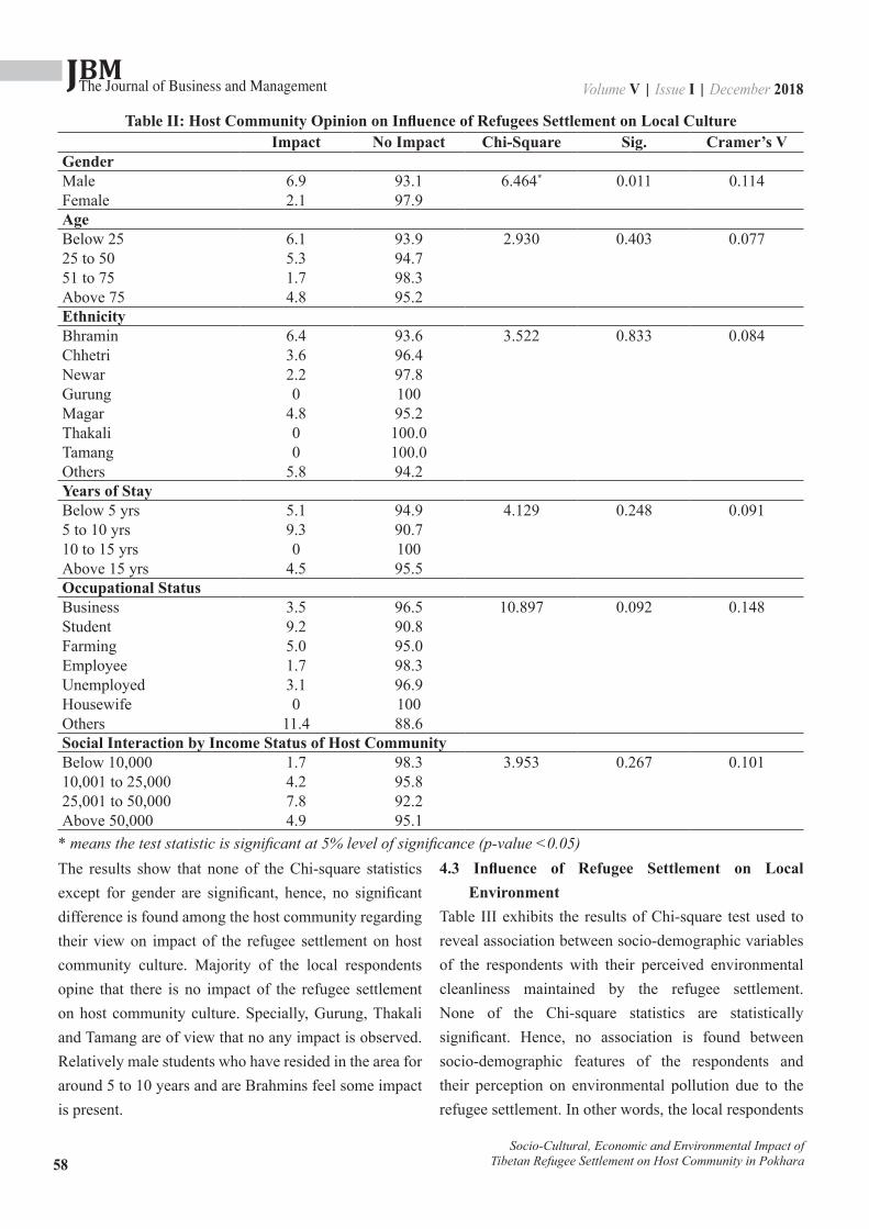
JBMVolume V | Issue I | December 2018The Journal of Business and Management
58
Table II: Host Community Opinion on Influence of Refugees Settlement on Local CultureImpact No Impact Chi-Square Sig. Cramer’s V
GenderMale 6.9 93.1 6.464* 0.011 0.114Female 2.1 97.9AgeBelow 25 6.1 93.9 2.930 0.403 0.07725 to 50 5.3 94.751 to 75 1.7 98.3Above 75 4.8 95.2EthnicityBhramin 6.4 93.6 3.522 0.833 0.084Chhetri 3.6 96.4Newar 2.2 97.8Gurung 0 100Magar 4.8 95.2Thakali 0 100.0Tamang 0 100.0Others 5.8 94.2Years of StayBelow 5 yrs 5.1 94.9 4.129 0.248 0.0915 to 10 yrs 9.3 90.710 to 15 yrs 0 100Above 15 yrs 4.5 95.5Occupational StatusBusiness 3.5 96.5 10.897 0.092 0.148Student 9.2 90.8Farming 5.0 95.0Employee 1.7 98.3Unemployed 3.1 96.9Housewife 0 100Others 11.4 88.6Social Interaction by Income Status of Host CommunityBelow 10,000 1.7 98.3 3.953 0.267 0.10110,001 to 25,000 4.2 95.825,001 to 50,000 7.8 92.2Above 50,000 4.9 95.1
* means the test statistic is significant at 5% level of significance (p-value <0.05)The results show that none of the Chi-square statistics except for gender are significant, hence, no significant difference is found among the host community regarding their view on impact of the refugee settlement on host community culture. Majority of the local respondents opine that there is no impact of the refugee settlement on host community culture. Specially, Gurung, Thakali and Tamang are of view that no any impact is observed. Relatively male students who have resided in the area for around 5 to 10 years and are Brahmins feel some impact is present.
4.3 Influence of Refugee Settlement on Local Environment
Table III exhibits the results of Chi-square test used to reveal association between socio-demographic variables of the respondents with their perceived environmental cleanliness maintained by the refugee settlement. None of the Chi-square statistics are statistically significant. Hence, no association is found between socio-demographic features of the respondents and their perception on environmental pollution due to the refugee settlement. In other words, the local respondents
Socio-Cultural, Economic and Environmental Impact of Tibetan Refugee Settlement on Host Community in Pokhara

JBMVolume V | Issue I | December 2018The Journal of Business and Management
59
have similar opinion regarding environmental hygiene maintained by the refugee settlement. Majority of
the respondents think that the Tibetan refugees have maintained environmental cleanliness.
Table III: Host Community Opinion on Influence of Refugee Settlement on Local EnvironmentYes No Chi-Square Sig. Cramer’s V
GenderMale 90.8 8.4 0.877 0.645 0.042Female 89.1 10.5AgeBelow 25 91.8 8.2 7.212 0.302 0.08525 to 50 88.3 11.351 to 75 90.4 7.8Above 75 100.0 0.0Years of StayBelow 5 yrs 89.7 10.3 3.723 0.714 0.0615 to 10 yrs 83.7 16.310 to 15 yrs 92.5 7.5Above 15 yrs 90.5 9.5Occupational StatusBusiness 91.5 8.5 16.699 0.161 0.129Student 93.8 6.2Farming 93.3 6.7Employee 85.0 15.0Unemployed 81.2 18.8Housewife 87.2 12.8Others 85.7 14.3
* means the test statistic is significant at 5% level of significance (p-value <0.05)
Overall, the results suggest that the Tashi Palkhiel settlement camp has not made adverse impact on the environment. The refugees have maintained environmental cleanliness, preserved natural resources and have not played role in environmental pollution. It means contrary to the findings of similar studies, the Tibetan camp at Hemja has been successful in preservation of the natural environment in their vicinity.
4.4 Influence of Refugee Settlement on Economic ActivitiesTable IV presents the association between socio-economic characteristics of the respondents and their perception on economic benefits received by the host community due the refugee settlement. The Chi-square statistics is found to be significant only in case of religion
and years of stay. It reveals that the view on whether the host community has received economic benefits in terms of increased business and employment opportunity is associated with religion and length of residency of the locals. The Chi-square value of 15.67 (p < 0.01) for the variable years of stay reveals that local residing in the study area for longer period of time perceive the local business and job opportunities have increased due to the refugee settlement. Similarly, the results reveal that Hindus and Christians have favorable view on economic benefits received by the host community due to refugee settlement. No association has been found in case of variables contact frequency, age, occupation and income level.
Socio-Cultural, Economic and Environmental Impact of Tibetan Refugee Settlement on Host Community in Pokhara
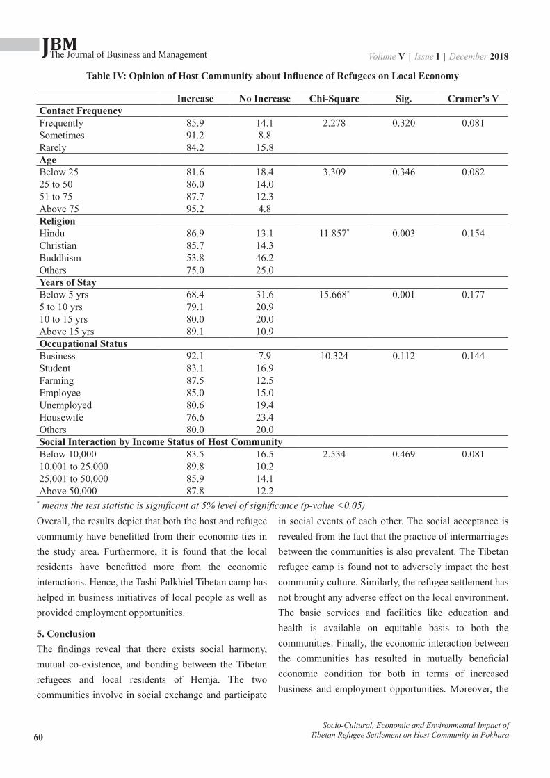
JBMVolume V | Issue I | December 2018The Journal of Business and Management
60
Table IV: Opinion of Host Community about Influence of Refugees on Local Economy
Increase No Increase Chi-Square Sig. Cramer’s VContact FrequencyFrequently 85.9 14.1 2.278 0.320 0.081Sometimes 91.2 8.8Rarely 84.2 15.8AgeBelow 25 81.6 18.4 3.309 0.346 0.08225 to 50 86.0 14.051 to 75 87.7 12.3Above 75 95.2 4.8ReligionHindu 86.9 13.1 11.857* 0.003 0.154Christian 85.7 14.3Buddhism 53.8 46.2Others 75.0 25.0Years of StayBelow 5 yrs 68.4 31.6 15.668* 0.001 0.1775 to 10 yrs 79.1 20.910 to 15 yrs 80.0 20.0Above 15 yrs 89.1 10.9Occupational StatusBusiness 92.1 7.9 10.324 0.112 0.144Student 83.1 16.9Farming 87.5 12.5Employee 85.0 15.0Unemployed 80.6 19.4Housewife 76.6 23.4Others 80.0 20.0Social Interaction by Income Status of Host CommunityBelow 10,000 83.5 16.5 2.534 0.469 0.08110,001 to 25,000 89.8 10.225,001 to 50,000 85.9 14.1Above 50,000 87.8 12.2
* means the test statistic is significant at 5% level of significance (p-value <0.05)Overall, the results depict that both the host and refugee community have benefitted from their economic ties in the study area. Furthermore, it is found that the local residents have benefitted more from the economic interactions. Hence, the Tashi Palkhiel Tibetan camp has helped in business initiatives of local people as well as provided employment opportunities.
5. ConclusionThe findings reveal that there exists social harmony, mutual co-existence, and bonding between the Tibetan refugees and local residents of Hemja. The two communities involve in social exchange and participate
in social events of each other. The social acceptance is revealed from the fact that the practice of intermarriages between the communities is also prevalent. The Tibetan refugee camp is found not to adversely impact the host community culture. Similarly, the refugee settlement has not brought any adverse effect on the local environment. The basic services and facilities like education and health is available on equitable basis to both the communities. Finally, the economic interaction between the communities has resulted in mutually beneficial economic condition for both in terms of increased business and employment opportunities. Moreover, the
Socio-Cultural, Economic and Environmental Impact of Tibetan Refugee Settlement on Host Community in Pokhara
JBMVolume V | Issue I | December 2018The Journal of Business and Management
61
economic benefits to the host community is relatively higher due to the refugee settlement. Overall, the findings reveal that Tashi Palkhiel Tibetan camp has positive impact on social, environmental and economic condition of the host community. The study selects only one Tibetan camp among twelve camps operating in Nepal. The study results will be more generalizable if more camps are included in the study. The study is based on opinion survey of only the local residents. Future studies can explore the issue by incorporating the perspectives
of the Tibetan refugees. Additionally, the study is based on quantitative research approach. In order to get better insights on the research issue, qualitative approach can be more appropriate. Inclusion of further dimensions of social, economic and environmental issues in the research study can offer more insightful findings in order to understand the phenomena. Acknowledgement: This article is the product of Faculty Research Award funded by University Grants Commission (UGC), Nepal in the year 2016.
Socio-Cultural, Economic and Environmental Impact of Tibetan Refugee Settlement on Host Community in Pokhara
Adisa, J. (1996). Rwandan Refugees and Environmental Strategy in the Great Lakes Region. A Report on the Habitat/UNEP Plan of Action. Journal of Refugee Studies, 326-334.
Alexander, A. (2010). Without Refuge: Chin Refugees in India and Malaysia. Retrieved from http://www.fmreview.org/FMRpdfs/FMR30/36-37.pdf
Alix-Garcia, J. (2007). The Effect of Refugee Inflows on Host Country Populations: Evidence fromTanzania. Retrieved from http://irnegotiation0708.pbworks.com/f/SSRN-id836147.pdf
Barth, F. (1994). Ethnic Groups and Boundaries. Retrieved from http://isites.harvard.edu/fs/docs/icb.topic446176.files/Week_4/Barth_Introduction_Et hnic_Groups_and_Boundaries_.pdf
Betts, A. (2006). Comprehensive Plans of Action: Insights from CIREFCA and the Indochinese CPA.Retrieved from http://www.unhcr.org/43eb6a152.pdf
Black, R., & Sessay, M. (1998). Forced Migration, Natural Resource Use and Environmental Change: The Case of the Senegal River Valley. International Journal of Population Geography, 31-47.
Buscher, D., & Heller, L. (2008). DesperateLives: Urban Refugee Women in Malaysia and Egypt.Retrieved from http://www.fmreview.org/en/urban-displacement/20-21.pdf
Chambers, R. (1986). Hidden Losers? The Impact of Rural Refugees and Refugee Programs on Poorer Hosts. International Migration Review, 245-263.
Commission, W. R. (2009). Peril or Protection: The Link Between Livelihoods and Gender based. Retrieved from www.womensrefugeecommission.org/images/stories/GBV_livelihoods_FINAL.pdf
Committee, U. S. (1998). Economic and Social Impact of Massive Refugee Populations on Host Developing Countries, as well as Other Countries: A Quantative Assessment on the Basis of Special Case Studies. UNHCR . Retrieved from http://www.unhcr.org/3ae68cf710.html
Crisp, J. (2003). No Solutions in Sight: The Problem of Protracted Refugee Situations in Africa. Retreved from http://www.unhcr.org/3e2d66c34.pdf
Dev, S. V. (2002). The Reluctant Host: The Socio-cultural Impact of Refugees on DevelopingCommunities. Mots Pluriel. Retrieved from http://motspluriels.arts.uwa.edu.au/MP2102s.html
Dolma, S., Singh, S., Lohfeld, L., Orbinski, J. J., & Mills, E. J. (2006). Dangerous Journey: Documenting the Experience of Tibetan Refugees. American Journal of Public Health , 2061-2064.
References

JBMVolume V | Issue I | December 2018The Journal of Business and Management
62
Ecology, N. A. (2010). Socio-economic and Environmental Impacts of Dadaab Refugee Camps on Host Communities. Retrieved from https://www.drc.dk/media/2108214/socio-economic-environmental-impact-study- of-the-dadaab-refugee-camp-on-the-host-community.pdf
Finnström, S. (2003). Living with bad surroundings: war and existential uncertainty in Acholiland, Northern Uganda (Doctoral dissertation, Acta Universitatis Upsaliensis). http://www.diva-portal.org/smash/record.jsf?pid=diva2%3A163495&dswid=-4457
Hakovirta, H. (1988). The Global Refugee Problem: A Model and Its Application. International PoliticalScience Review (1993) , 35-57.
Hamza, B. M. (2006). A report on the Somali remittance sector in Canada: Prepared for Nathanson Centre for the Study of Organized Crime and Corruption. Retrieved from https://www.library.yorku.ca/find/Record/2036598
Jacobsen, K. (1996). Factors Influencing the Policy Responses of Host Governments to Mass Refugee Influxes. The International Migration Review , 655-678. Retrieved from europepmc.org/abstract/MED/12292015
Kandoh, M. M. (2012). Forced Migration: Socio-economic Implications for Hosts Communities in Southern and Northern Ghana. Retrieved from www.hioa.no/content/download/17625/190127/file/MorforKandoh.pdf
Martin, A. (2005). Environmental Conflict Between Refugee and Host Communities. Journal of Peace Research , 329–346.
Maystadt, J.-F., & Verwimp, P. (2009). Households in Conflict Network (Working Paper 60): Winners and Losers among a Refugee-Hosting. The Institute of Development Studies - at the University of Sussex - Falmer - Brighton - BN1 9RE. Retrieved from http://www.hicn.org/
wordpress/wp-content/uploads/2012/06/wp60.pdf
Miller, S. D. (2018). Assessing the Impacts of Hosting Refugees. Centre for International Governance Innovation World Refugee Council , 1-13.
Mills, E. J., Singh, S., Holtz, T. H., Chase, R. M., Dolma, S., Barbara, J. S., et al. (2005). Prevalence of mental disorders and torture among Tibetan refugees: A systematic review. BMC International Health and Human Rights , 1-8.
Mekuria, W. (2013). The Socio-Economic Impact of South Sudanese refugees on the Host Community in Ethiopia: the Case of Pugnido Refugee Camp: Pugnido, Gambella Region. Retrieved from http://etd.aau.edu.et/bitstream/123456789/6051/1/13.%20Woenu%20Mekuria.pdf
NUCRA. (2010). Refugees in Nepal: A Short Glimpse. Leaflet
Omeokachie, I. V. (2014). The Security implications of the refugee situation in South Africa. MA Thesis, University of Pretoria).Retrieved from https://repository.up.ac.za/bitstream/handle/2263/41367/Omeokachie_Security_2014. pdf?sequence=1
Paljor, T. (2007). Current Situation of Tibetan Refugees in Exile. Retrieved from geography.org.uk/download/GA_Conf07Paljor.doc
Pini, J. (2008). Political Violence and the African Refugee Experience. International Affairs Review. Retrieved from http://www.iar-gwu.org/node/19
Schmeidl, S. (1997). Exploring the Causes of Forced Migration: A Pooled Time-Series Analysis, 1971-1990. Social Science Quarterly, 284-308.
Smith, M. P. 2001 “Preface.” In New Approaches to Migration? Transnational Communities and the Transformation of Home. Ed. N. Al-Ali and K. Koser. London: Routledge.
Socio-Cultural, Economic and Environmental Impact of Tibetan Refugee Settlement on Host Community in Pokhara

JBMVolume V | Issue I | December 2018The Journal of Business and Management
63
TJC. (2002). Tibet’s Stateless Nationals: Tibetan Refugees in Nepal. Retrieved from http://www.tibetjustice.org/reports/nepal.pdf
UNHCR. (1997). Economic and Social Impacts of Massive Refugee Populations on Host Developing Countries, as well as other Countries. Standing Committee. UNHCR, EC/47/SC/CRP.7. Retrieved from https://www.unhcr.org/excom/standcom/3ae68d0e10/social-economic-impact-large- refugee-populations-host-developing-countries.html
Werker, E. (2007). Refugee Camp Economies. Journal of Refugee Studies. Retrieved from http://www.humanitarianinnovation.com/uploads/7/3/4/7/7347321/werker_2007.pdf
Whitaker, B. E. (1999). Changing opportunities: Refugees and Host Communities in Western Tanzania. Retrieved from http://www.unhcr.org/3ae6a0c70.pdf
Whitaker, B. E. (2002). Refugees in Western Tanzania: The Distribution of Burdens and Benefits Among Local Hosts. Journal of Refugee Studies. Retrieved from https://clas-pages.uncc.edu/beth-whitaker/files/.../whitaker-JRS-2002.pdf
Zetter, R. (1995). Incorporation and Exclusion: The Life Cycle of Malawi’s Refugee Assistance Program.World Development, Key: citeulike:8953803 , 1653- 1667.
Zetter, R., & Deikun, G. (2010). Meeting Humanitarian Challenges in Urban Areas: Migration Review issue. Retrieved from file:///E:/course/onsite%20sanitation/zetter-deikun-05-07.pdf
Socio-Cultural, Economic and Environmental Impact of Tibetan Refugee Settlement on Host Community in Pokhara

JBMVolume V | Issue I | December 2018The Journal of Business and Management
64
1. Introduction Nepalese capital market is dominated by financial sector and is characterized by inefficient management, low volume of transactions, unhealthy competition, lack of competitive strength, lack of project financing, lack of skilled human resources, etc. Merger is an appropriate way to overcome these deficiencies. On other hand, Nepal government has opened the door for foreign banks and institutions after becoming the member of WTO. When there is good political and economic environment, no doubt; any time foreign banks would come up with high technical and capital resources. This situation will obviously create competitive pressures for domestic banks. Nepalese government has been offering various supportive policy levels to go for merger and Nepal Rastra Bank also been encouraging the bank and
financial institution for institutionalising the merger and acquisition. Therefore, from strategic view point, the initiative of Nepal government the and NRB for proactive measures to safeguard the position of domestic banks should be appreciated. Nevertheless, with increased liberalization and economic reforms in some countries in the region, more and more banks are getting merged for various reasons. The trend towards merger and acquisition has just started in Nepal from last decade. Laxmi bank merger with HISEF finance in 2004 is a significant milestone in the Nepali corporate sector. Later Nepal Bangladesh bank was merged with NB finance (within same group) in 2007. Likewise, H&B Development Bank came into existence after a merger between Himchuli Finance and Birgunj Finance. Kasthamandap Finance amalgamated with
Event Study of Effect of Merger Announcement on Stock Price in NepalShanti Devi Chhetri1 , Ravindra Prasad Baral2
Abstract
Events like merger and acquisition affect the value of merging firms and also generate a positive or negative wealth effect for shareholders of firms involved. The purpose of this study is to investigate whether a merger announcement has generated wealth effects for the shareholders of bidding and target firms as well as it has aimed to assess the impact on overall banking sector. Two models; mean adjusted model and market risk adjusted model has been used in the study employing the ‘event study’ methodology to examine whether there is presence of abnormal return associated with merger announcement. In this method, 50 days premerger and 30 days post merger period is assumed as estimation period and (-15 and +15 ) days are taken as the window period. Fifteen financial institutions which entered into merger between years 2010 to 2012 are selected as sample. The findings of this study demonstrated that surrounding the announcement of merger proposals, the premerger abnormal return of individual firms is not significant to zero i.e. return is not affected by the merger announcement. Similarly, the abnormal return of bidding and target firms is not significant which indicates there is no impact of merger announcements on shareholder wealth in Nepalese capital market. Finally, the abnormal return during the premerger and post merger period of individual firms as well as the overall banking sector shows the same result, there is no significant difference on return before and after the merger announcement.
Keywords: Abnormal Stock Return, Capital Market, Merger and Acquisition, Signalling Effect
ISSN 2350-8868
1. Lecturer, School of Business, Pokhara University2. Lecturer, School of Business, Pokhara University
JBMVolume V | Issue I | December 2018The Journal of Business and Management
65
Shikhar Finance to become Kasthamandap Development Bank. A merger between Business Development Bank and Universal Finance resulted in the formation ofBusiness Universal Development Bank
Banking reforms have allowed banks to engage in voluntary M&A which has led to high consolidating activity in the banking sector. The sample and methodology of this paper focused to see the relationship between merger announcement and stock returns.
The need for constant change in today’s dynamic business environment propels the companies to look for expansion by acquisition or merging with other companies (Shah & Arora, 2014). With the entry of new private banks, the domestic banks have been facing the pressure of competition. This is one reason why consolidation could be an imperative for Nepalese banks. Higher capital adequacy ratio of a bank indicates its potential for growth, financial solvency and ensures confidence for depositors. Capital deficient bank are unable to grow unless they augment the capital resources (Jayadev & Sensarma, 2007). The way out of this problem is to merge capital deficient bank with a bank of stronger capital base. In order to mitigate the risk of large capital inflows due to full convertibility of rupee on capital account, strong and large banks are needed and their evolvement is possible through consolidation.
Many banks are operating in urban areas, there is high competition on these areas and equally there is a regulatory pressure to expand services in rural part of the country. Banks that have already reached at rural areas and other which has to reach for business expansion; consolidation of banks through merger has been preferred choice for banks to grow and become big. From last few years, Nepalese banks have suffered from high liquidity crisis, many banks became problematic and some were closed down. To maintain the profitability and reduce competitive pressures, bank need to expand their services. Thus, through the merger and acquisition it has easier to go economies of scale for growth and profitability. Wong and Cheung (2009) indicates that corporate takeover is good news for the shareholders of bidding firms but not
regarded as good news for the shareholders of the target firms. In addition, researchers confirm the hypothesis that the abnormal return for the shareholders of bidding firms during the post-announcement period depends on the type of acquisition. The existing empirical literature available on corporate restructuring events in Nepal and their effects on shareholders’ value is scanty; hence, there is a need for more studies on the subject. This study will help researchers to understand the concept of event study methodology and encourage analyzing the impact of corporate restructuring on stock returns. The main objective of this study is to assess the impact of merger announcement effect on share price and abnormal returns of financial institutions of Nepal during the pre and post merger announcement period. This study analyzes stock price behaviour before and after merger activity. It examines the abnormal return of each institution’s share price pre and post merger. It compares the impact of merger announcement on the acquirer and target firms’ stock price. The study focus on whether M&A in the Nepalese banking sector, spurred by the banking reforms, have actually improved bank performance for those banks involved. The stock price is related to only merger event. Specifically, the study adds to the merger literature related to signalling effect of merger announcement on value of the target and acquiring firm.
2. Literature ReviewKhan and Ikram (2012) conducted the study with objective to test the efficiency of the Indian Stock Market with respect to the announcement of mergers and acquisition in the Indian Banking Sector by employing the standard Risk Adjusted Event Study Methodology. Their studies show the efficiency of the market in its semi strong form of EMH by accepting both the null hypothesis. It is observed that neither before nor after the merger announcement investors are able to earn abnormal/excess return. Padmavathy and Ashok (2012) investigated the informational value of merger announcement to the shareholders to earn abnormal return. The study concluded that a merger announcement does not hold important information to the Indian stock market during the study period. Return from the
Event Study of Effect of Merger Announcement on Stock Price in Nepal

JBMVolume V | Issue I | December 2018The Journal of Business and Management
66
announcement of merger and therefore the shareholders don’t reap any abnormal return.
Anand and Jagandeep (2008) have conducted the research on impact of merger announcements on shareholders. Wealth: Evidence from Indian private sector banks. This research report positive merger effects on the total wealth of shareholders in the private banking industry. Joshua (2011) attempted to make a comparative analysis of the impact of mergers and acquisitions on financial efficiency of selected banks in Nigeria. It was found that the post mergers and acquisitions’ period was more financially efficient than the pre-mergers and acquisitions period.
Bhardwaj (2014) studied with the objective to find out whether the merger and acquisition deal between the two banks ie (Centurion Bank and Bank of Punjab ) was successful or not ? The researcher concluded was that the merger activity has become good for both the banks, the overall efficiency and the productivity increases over the years. Sinha, Kaushik, and Chaudhary (2010) examined the impact of mergers and acquisitions on the financial efficiency of the selected financial institutions in India. The result of the study indicate that M&A cases in India show a significant correlation between financial performance and the M&A deal, in the long run, and the acquiring firms were able to generate value.
Gattoufi, Al-Muharrami, and Al-Kiyumi (2009) researched on the impact of mergers and acquisitions on the efficiency of GCC banks. The major result was that, though it was limited, there was a positive impact of M&A on the performance of commercial banks. Moreover, most of the banks involved in M&A realized an improvement higher than the average realized by the full sample, and hence improved their performances faster than the market. Mahmood, Aamir, Hussain, and Sohail (2012) studied the impact of merger/ acquisition on share price - A case study of Pakistan. The results indicate that M&A positively affect the share price of companies.
Sinha and Gupta (2011) studied mergers & acquisitions scenario of the Indian financial services sector. From the study it can be concluded that the M&A activity
in the Indian financial services sector over a period of March 1993- Feb 2010 has had positive effects on the profitability in majority cases but the liquidity position has deteriorated in a period of three years after the merger. Liargovas and Repousis (2011) examined the impact of mergers and acquisitions on the performance of Greek banking sector. The overall results (the weighted average of gains to the bidder and target bank), indicated that bank mergers and acquisitions have no impact and do not create wealth.
3. Data and Methodology
3.1 Nature of Data and SamplingThis study is based on secondary data. The data for mergers and acquisitions is taken from the Nepal Stock Exchange; however, some of merged companies have been delisted by the NEPSE, thus, the Pre merger data of each firm were taken from merolagani.com. Based on the availability of data, following Bank and Financial Institution are selected as sample for the study:
Table I: Sample M & A Events
S.N Pre MergerName
Trading Halt Date AtNEPSE
Post MergerName
1
BusinessDevelopmentBank
29-09-2011
BusinessUniversal DevelopmentBankLtd
Universal Finance 13-09-2011
2Himchuli BikashBank 03-03-2011 H&B Bank Ltd
Birgunj Finance 03-03-2011
3. MBL 11-12-2011 MacchapuchhreBankLtd
Standard Finance 11-12-2011
4
Global bank ltd 02-02-2012 Global IMEIME 02-02-2012Lord BuddhaFinance 09-10-2011
5KastamandapBank 19-06-2011
Kastamandap DevelopmentBankLtd
Shikhar Finance NA
Event Study of Effect of Merger Announcement on Stock Price in Nepal

JBMVolume V | Issue I | December 2018The Journal of Business and Management
67
All of the firms that have gone for merger in Nepalese history has been tried to bring under the study area. However, the companies that have already been delisted from the NEPSE made difficulty to get all price history for the study. Thus, on the basis of data availability, those banks and financial institution that have gone on merger process from January 1, 2010 to December 1, 2012 and have 30 days trading history after the merger completion are taken as a sample. Along with this we have assumed t=0 as an announcement period for the date at which individual bank’s trading has stopped or halted at NEPSE.
3.2 Event Study Method
Event studies method is arguably the best available instrument for measuring the impact of particular event on the phenomena. At any given point in time, security prices might be affected by a large number of randomly generated pieces of new information or events. Here the phenomenon is the shareholder return and merger is the event that could have impact on the shareholder perceptions and motives.
Figure I : Event Windows
Reason for Choosing the 15 Day MeasurementThe reason for choosing a 15 day measurement before and after the announcement is that the Nepalese capital market is not efficient even in weak form. Therefore, there is very few information as publicly available. And in case of merger in Nepal, merger practices are new. Merger proposal has to be passed from the general meetings but the partner is not defined. General meeting gives authority to board to conduct due diligence audit and choose the partner. The board conduct audit to find possible partner. From the day of audit they both request NEPSE to halt their share trade. In such case investor are informed only after the share halt. They play with
the rumours till the official announcement of merger. Therefore, more the event period is taken, more the shareholder or investor are informed and confirmed about the events. In such conditions, 15 day measurement before the announcement is important in order to detect any price movement as a result of any rumours of merger proposals.
3.3 The Market ModelIn this method, value of α and β are calculated from the estimation period. After this, forecast of the return of individual security can be done. εt is the estimation of residual value from which we calculate the abnormal return of a security. Share price performance from the event t=-50 to -15 to t= 15 to 30 days is used to estimate the parameters of the market model, and the abnormal rate of return of the merging firms during the window period (pre and Post announcement period) is estimate using the parameter. The abnormal return captured by residual’s of firm i on day t is expressed as
et = α+ β Rmt ... ... ... ... (1)Where:Rt = daily share return for firm / in day t α = the intercept
termβ = the systematic risk of shareRmt = rate of return on a market index in day t relative to
the announcement of offeret = residual termt = - 15 . . . +15 daysThe daily share return, Rt can be calculated from the formula:
Rt = (P1 – P0) /P0 ............ (2)t = - 15. . . +15 days
Where:P1 = price per share of common stock of firm / at the end of day tP0 = price per share of common stock of firm / at the end of day t-1
Market Retum, Rmt. Can be calculated from the formula
Rmt = (M1 – M0)M0 ... ... ... (3) t = - 15 ,. . . , +15 days
Event Study of Effect of Merger Announcement on Stock Price in Nepal

JBMVolume V | Issue I | December 2018The Journal of Business and Management
68
where:M1 = stock market index at the end of day / M0 = stock market index at the end of day t-1
The abnormal returns for firm I / in day t, ARdit, based on the market model can be defined as:
ARt = Rt – α- β Rm t ... ... ... (4)OR
ARt = Rt - et
whereet and Rt for individual firm are calculated daily by using the equation (1) and (2) from the event t=-15 to t= 15 days.
The cumulative abnormal return, CAR i, for the bidders and the target firms for the period of t = - 15 to t = 15 can be defined as :
CARi= ∑AR ..........(5)
N
t-1
3.4 The Mean adjusted modelThe Mean adjusted model is practically simpler than the market model; it is widely used as a comparison for the market model for some research on event studies. In this model we assumed that the normal return forthe a security equals a constant Kt (Mean Value ) over the estimation period. The expected return for the security is assumed to be constant over time, though ex-ante return will vary among securities. Thus, abnormal return for the security is found:
ARt = Rt - Kt ... ... ... ... (6)Where,Rt = day of return on day tKt = Mean value of the daily return
Daily return can be calculated as:Rt = (P1 – P0) /P0 ... ... ... ... (7)
Where,P1 = price per share of common stock of firm / at the end
of day tP0 = price per share of common stock of firm / at the end
of day t-1t = - 15. . . +15 days
The cumulative abnormal return, CAR i, for the bidders
and the target firms for the period of t = - 15 to t = 15 can be defined as:
CARt = ∑AR .......... (8)N
t-1
3.5 Hypotheses DevelopmentThe study attempts to analyze whether merger announcement made by both bidder and target companies have significant impact on the company’s stock returns. Different t-tests (one sample t-test, independent sample t-test) is used to test the hypothesis presented below. To test for the significance for individual firms, one sample t-test has been conducted in which we have set the following hypothesis assumption:-
H1: Merger announcement have a significant impact on stock returns.
H1: AR ≠ 0
To test the difference in mean abnormal return between target and acquiring firm; Pre and Post merger impact, the Independent Sample T- test has been conducted for testing equality of mean returns.
H2: Merger announcement have significant impact on stock returns between the firms or Pre merger return and Post merger return.
H2: ARFirm(A) ≠ AR(FirmB) OR AR(Pre) ≠ AR(Post)
4. Empirical AnalysisThe Table II exhibits the abnormal return and cumulative abnormal returns calculated using the market adjusted model and mean adjusted model. The values are calculated for the event window period of 15 days. The t-test result is also presented to test if the abnormal returns are significantly different from zero. It is expected that if the positive signalling effect from merger announcement is present than the abnormal stock returns during the period will be positive.
Table II reveals that the average abnormal return (AR) of overall firms from both mean adjusted and Market adjusted models. There is positive return of 0.02501 and 0.02855 after the merger announcement from both models. While we compare the return from both model, we can found highest return from mean model on day
Event Study of Effect of Merger Announcement on Stock Price in Nepal
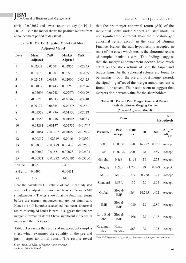
JBMVolume V | Issue I | December 2018The Journal of Business and Management
69
(t=4) of 0.03089 and lowest return on day (t=-10) is -.03281. Both the model shows the positive returns from announcement period to day (t=4).
Table II: Market Adjusted Model and Mean Adjusted Model
Days Mean Adjusted
CAR Market Adjusted
CAR
1 0.02501 0.02501 0.02855 0.02855
2 0.01400 0.03901 0.00570 0.03425
3 0.02453 0.06354 0.02000 0.05425
4 0.03089 0.09443 0.02250 0.07676
5 -0.02696 0.06748 -0.02976 0.04699
6 -0.00715 0.06033 -0.00860 0.03840
7 0.00322 0.06355 -0.00278 0.03561
8 -0.01358 0.04996 -0.01533 0.02028
9 -0.01558 0.03438 -0.01045 0.00983
10 -0.03281 0.00157 -0.02732 -0.01749
11 -0.01864 -0.01707 -0.01057 -0.02806
12 -0.00812 -0.02519 -0.00164 -0.02971
13 0.01030 -0.01489 0.00439 -0.02531
14 -0.00062 -0.01551 0.00028 -0.02503
15 -0.00321 -0.01872 -0.00596 -0.03100
t value -0.251 -.478
Std error 0.0496 0.00431
sig. .805 .640
Here the calculated t – statistic of both mean adjusted and market adjusted return models is -.805 and -.640 simultaneously. The test shows that the abnormal returns before the merger announcement are not significant. Hence the null hypothesis accepted that means abnormal return of sampled banks is zero. It suggests that the pre merger information doesn’t have significant influence in increasing the stock price.
Table III presents the results of independent samples t-test which examines the equality of the pre and post merger abnormal return. The results reveal
that the pre-merger abnormal return (AR) of the individual banks under Market adjusted model is not significantly different than their post-merger abnormal return except in the case of Birgunj Finance. Hence, the null hypothesis is accepted in most of the cases which means the abnormal return of sampled banks is zero. The findings suggest that the merger announcement doesn’t have much effect on the stock returns of both the target and bidder firms. As the abnormal returns are found to be similar in both the pre and post merger period, the signalling effect of the merger announcement is found to be absent. The results seem to suggest that mergers don’t create value for the shareholders.
Table III : Pre and Post Merger Abnormal Return Analysis between Merging Partner
(Market Adjusted Model)
Firm Null Hypothesis
Premerger Post merger
t- statis-tics Df Sig ARpre =
ARpost
BDBL BUDBL 0.88 16.227 0.931 Accept
UF BUDBL .700 28 .489 Accept
Himchuli H&B -1.161 28 .255 Accept
Birgunj H&B -1.705 28 0.099 Reject
MBL MBL .903 20.258 .377 Accept
Standard MBL -.137 28 .892 Accept
Global Global-IME -.864 14.265 .402 Accept
IME Global-IME 1.080 28 .289 Accept
Lord Bud-dha
Global-IME 1.496 28 .146 Accept
Kastaman-dav
Kasta-mandav -.863 28 .395 Accept
Note: Null hypothesis ARpre = ARpost : Premerger AR is equal to Post merger AR
Event Study of Effect of Merger Announcement on Stock Price in Nepal
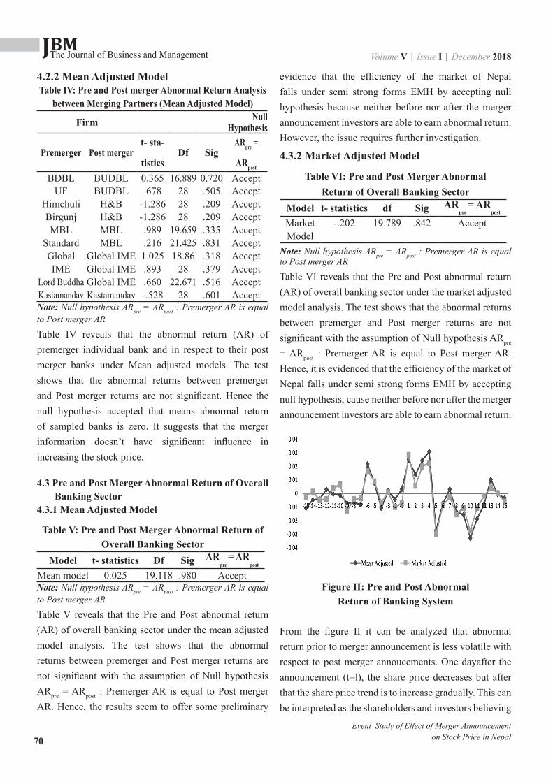
JBMVolume V | Issue I | December 2018The Journal of Business and Management
70
4.2.2 Mean Adjusted ModelTable IV: Pre and Post merger Abnormal Return Analysis
between Merging Partners (Mean Adjusted Model)
Firm Null Hypothesis
Premerger Post mergert- sta-
tisticsDf Sig
ARpre =
ARpost
BDBL BUDBL 0.365 16.889 0.720 AcceptUF BUDBL .678 28 .505 Accept
Himchuli H&B -1.286 28 .209 AcceptBirgunj H&B -1.286 28 .209 AcceptMBL MBL .989 19.659 .335 Accept
Standard MBL .216 21.425 .831 AcceptGlobal Global IME 1.025 18.86 .318 AcceptIME Global IME .893 28 .379 Accept
Lord Buddha Global IME .660 22.671 .516 AcceptKastamandav Kastamandav -.528 28 .601 AcceptNote: Null hypothesis ARpre = ARpost : Premerger AR is equal to Post merger ARTable IV reveals that the abnormal return (AR) of premerger individual bank and in respect to their post merger banks under Mean adjusted models. The test shows that the abnormal returns between premerger and Post merger returns are not significant. Hence the null hypothesis accepted that means abnormal return of sampled banks is zero. It suggests that the merger information doesn’t have significant influence in increasing the stock price.
4.3 Pre and Post Merger Abnormal Return of Overall Banking Sector
4.3.1 Mean Adjusted Model
Table V: Pre and Post Merger Abnormal Return of Overall Banking Sector
Model t- statistics Df Sig ARpre
= ARpost
Mean model 0.025 19.118 .980 AcceptNote: Null hypothesis ARpre = ARpost : Premerger AR is equal to Post merger ARTable V reveals that the Pre and Post abnormal return (AR) of overall banking sector under the mean adjusted model analysis. The test shows that the abnormal returns between premerger and Post merger returns are not significant with the assumption of Null hypothesis ARpre = ARpost : Premerger AR is equal to Post merger AR. Hence, the results seem to offer some preliminary
evidence that the efficiency of the market of Nepal falls under semi strong forms EMH by accepting null hypothesis because neither before nor after the merger announcement investors are able to earn abnormal return. However, the issue requires further investigation.
4.3.2 Market Adjusted Model
Table VI: Pre and Post Merger Abnormal Return of Overall Banking Sector
Model t- statistics df Sig ARpre
= ARpost
Market -.202 19.789 .842 AcceptModel
Note: Null hypothesis ARpre = ARpost : Premerger AR is equal to Post merger ARTable VI reveals that the Pre and Post abnormal return (AR) of overall banking sector under the market adjusted model analysis. The test shows that the abnormal returns between premerger and Post merger returns are not significant with the assumption of Null hypothesis ARpre = ARpost : Premerger AR is equal to Post merger AR. Hence, it is evidenced that the efficiency of the market of Nepal falls under semi strong forms EMH by accepting null hypothesis, cause neither before nor after the merger announcement investors are able to earn abnormal return.
Figure II: Pre and Post Abnormal Return of Banking System
From the figure II it can be analyzed that abnormal return prior to merger announcement is less volatile with respect to post merger annoucements. One dayafter the announcement (t=l), the share price decreases but after that the share price trend is to increase gradually. This can be interpreted as the shareholders and investors believing
Event Study of Effect of Merger Announcement on Stock Price in Nepal
JBMVolume V | Issue I | December 2018The Journal of Business and Management
71
that merger proposals will generate some advantages. This situation also create optimism in shareholders and investors that the merger proposal will drive up the value of their shares which in tum will maximise their wealth effect.
Certain empirical evidence indicates substantial excess returns to the stockholders of the target company after the merger announcement. This wealth increment is due to the premium paid by the acquiring company for the target and synergistic benefits expected to occur due to merger. Typically, the stock price improvement begins prior to the merger announcement. However, for the acquiring company stockholders, the evidence is mixed. For acquiring company the premium paid for the target and its justification in terms of expected synergy and more efficient management of the resources of the target company determines the abnormal returns. This study reveals that the abnormal returns due to merger announcements are not significant and the pre and post merger abnormal returns are not significantly different. The results reveal that merger announcement in Nepal don’t create value for both the merging firms. The positive signalling effect of merger announcement is absent. The theoretical justification of the result is that the stock market of Nepal is not efficient even in weak form. Hence, the information on merger announcement is not fully reflected in share prices of the target and bidding company.
5. Conclusion From market adjusted model, the abnormal return of global bank is higher than the other firms where as IME have lowest and negative abnormal returns. According to the mean adjusted model, IME has the highest abnormal return among the merging companies. However, the assumption of merger impacts on shareholder’s return (AR=0) has been proved caused none of the firms is significant on the basis of analysis. Since the abnormal return of individual bank has been proved as an insignificant, between the merging partner and the abnormal return between the bidder and target firms also found as there is no significance difference on
shareholder’s return due to the merger announcement. Here in context to Nepal, the investor’s motive has not changed on the merging firm’s size, growth and profitability either investor are less informed about the market events. This result has proved that, an involuntary merger activity has not able to grab the attention of investors. Similarly, the Mean adjusted model analysis of abnormal returns between the firm’s pre merger announcement and post merge announcement also, the results are proved according to our assumption i.e. none of the firm’s pre merger abnormal returns different in respect to their post merger firms. While according to the market adjusted model, pre merger Birgunj finance’s abnormal return is different in respect to its post merger firms i.e. H&B. Except the Birgunj and H&B, other firm’s abnormal return between pre and post merger are equal. The entire firm’s test statistics depicts that the null hypothesis is accepted in an assumption of pre merger abnormal return of firms is equal to the post merger abnormal return. The test statistics is insignificant in all cases of selected firms, so it clear that the announcement of merger news has not made impacts on the investor’s perceptions and motives. While talking the merger impacts on overall banking system, from aspects of both Mean and Market adjusted model also the entire firm’s test statistics depicts that the null hypothesis is accepted in an assumption of pre merger abnormal return of firms is equal to the post merger abnormal return. The test statistics is insignificant in all cases of overall banking sector, so it clear that the announcement of merger news has not made impacts on the investor’s perceptions and motives. For strengthen the banking sector, NRB is using the various policies and directives. Involuntarily merger concept is not working; the investors and bankers are not willing in favour of merger policies in such conditions the impact is less effective. And another reality of no impacts on shareholder is, inappropriate partners. Partners should be chosen from same category. Same class partnership could create great impacts on shareholder’s returns. Banks are just fulfilling the compliances of NBB’s Directives not for gaining the advantages of synergy impacts. This study was conducted with the aim to find the market
Event Study of Effect of Merger Announcement on Stock Price in Nepal

JBMVolume V | Issue I | December 2018The Journal of Business and Management
72
efficiencies, the evidence here supports the efficiency of the market in its semi strong from of EMH by accepting both pre and post merger null hypothesis. It is observed that neither before nor after the merger announcement investors are able to earn abnormal/ excess return. Similarly the hubris theory assumptions are not found in Nepalese capital market. Random abnormal returns are found in between the return of bidder and target.At the end it is concluded that the merger practices do not have positive impact on shareholders return. Pre merger abnormal return is not significant with the post merger abnormal return. Neither before nor after the merger announcement, were investors able to earn abnormal
return. From the study it can be inferred that in context of Nepal, a merger activity is unable to create positive impacts on shareholder perception and motives.
This study is significant not only to the shareholders who are an important stakeholder of a banking firm but also to policy makers because in a country like Nepal where public sector banks dominate the banking industry, it is the Government who is the major owner of such enterprises and will incur financial loss if mergers are not creating any wealth. Most of the bank mergers in Nepal are policy driven and not market driven, hence it is important for the policy makers to understand that their policies have added value for all the stakeholders or not.
Event Study of Effect of Merger Announcement on Stock Price in Nepal
ReferencesAnand, M., & Jagandeep, S. (2008). Impact of Merger
Announcements on Shareholders’ Wealth: Ev-idence from Indian Private Sector Banks. Jour-nal for Decision Makers , 35-54.
Andrade, G., Mitchell, M., & Stafford, E. (2001). New Evidence and Perspectives on Mergers. Journal of Economic Perspectives , 103–120.
Bhardwaj, M. M. (2014). A study of Merger and ac-quisition between Centurion Bank with Bank of Punjab: Analysing Premerger and Postmerger Financial Performance. International Journal of In-novation and Scientific Research , 50-63.
Calipha, R., Tarba, S., & Brock, D. (2010). Mergers and Acquisitions: AReview of Phases, Motives, and Success Factors. Advances in Mergers and Acqui-sitions , 1-24.
Fama, E. F. (1998). Market Efficiency,Long-term Returns, and Behavioral Finance. Journal of Financial Economics, 283-306.
Focarelli, D., Panetta, F., & Salleo, C. (2002). Why Do Banks Merge? Journal of Money, Credit and Bank-ing , 1047-1066.
Gattoufi, S., Al-Muharrami, S., & Al-Kiyumi, A. (2009). The Impact of Mergers and Acquisitions on the Efficiency of GCC Banks. Banks and Bank Systems, 94-101.
Healy, P. M., Palepu, K. G., & Rubak, R. C. (1990). Does Corporate Performance Improve After Mergers? The National Bureau of National Research , 135-176.
Jayadev, M., & Sensarma, R. (2007). Mergers in In-dian Banking: An Analysis[dagger]. South Asian Journal of Management . Retrieved from https:// www.questia.com/.../mergers-in-indian-bank-ing-an-analysis-dagger
Joshua, O. (2011). Comparative Analysis of the Impact of Mergers and Acquisitions on Financial Effi-ciency of Banks in Nigeria. Journal of Accounting and Taxation , 1-7.
khan, A. A., & Ikram, S. (2012). Testing the Efficien-cy of Indian Stock Market Vis-ÀVis Merger and Acquisitions - A Study of Indian Banking Sector. International Journal of Latest Trends in Finance & Economic Sciences , 155-168.
Liargovas, P., & Repousis, S. (2011). The Impact of Mergers and Acquisitions on the Performance of the Greek Banking Sector: An Event Study Ap-proach. International Journal of Economics and Finance , 89-100.
JBMVolume V | Issue I | December 2018The Journal of Business and Management
73
Mahmood, I., Aamir, M., Hussain, M., & Sohail, N. (2012). Impact of Merger/ Acquisition on Share Price - A CaseStudy of Pakistan. European Jour-nal of Scientific Research , 617-624.
Padmavathy, D. S., & Ashok, D. J. (2012). Merger Announcements and Stock Price Behavior: Em-pirical Evidence from Indian Stock Market. Inter-national Research Journal of Finance & Economics 153-160.
Shah, P., & Arora, P. (2014). M&A Announcements and Their Effect on Return to Shareholders: An Event Study. Accounting and Finance Research , 170-190. Retrieved from http://dx.doi.org/10.5430/afr. v3n2p170
Sinha, D. N., Kaushik, D. K., & Chaudhary, M. T. (2010). Measuring Post Merger and Acquisition Perfor-mance: An Investigation of Select Financial Sector Organizations in India . International Journal of Economics and Finance , 190-200.
Sinha, P., & Gupta, S. (2011). Mergers and Acquisitions: A pre-post analysis for the Indian financial ser-vices sector. Munich Personal RePEc Archive , 2-36. Retrieved from https://mpra.ub.uni-muenchen.de/31253/1/MPRA_paper_31253.pdf
Wong, A., & Cheung, K. Y. (2009). The Effects of Merger and Acquisition Announcements on the Security Prices of Bidding Firms and Target Firms in Asia. International Journal of Economics and Finance , 274-283.
Event Study of Effect of Merger Announcement on Stock Price in Nepal
JBMVolume V | Issue I | December 2018The Journal of Business and Management
74
Influence of Demographic Factors on Job Satisfaction of Financial Institutions
Workforce of NepalIndira Shrestha1
AbstractThis paper examines the influence of demographic factors on job satisfaction of employees of Nepalese Financial Institutions. The survey instrument was distributed to the employee of commercial banks, development banks and finance companies located at Lekhnath municipality and Pokhara Sub-metropolitan city. The sample size for this study was 150. The sample was selected using strati-fied sampling. This study presented communication, career development, and role of employee, working condition, recognition, and reward, immediate supervisor, and training pro-gram as factors of job satisfaction. Data were analyzed by using statistical tools like frequency, mean, and percentage. Moreover to test the hypothesis presented in this study, independent t-test, ANOVA analysis have been used. This research concluded that demographic variables (gender, job position, and age) influence the level of job satisfaction of employees of Nepalese financial institutions.
Keywords: Demographic Factors, Job Satisfaction, Nepalese Financial Institutions
1 Lecturer, Tribhuvan University
1. Introduction Financial institutions of Nepal are playing important role in the overall economic development of country. In Nepal financial institutions have been growing in sufficient number after the declaration of liberal policy related to financial institutions by Nepal Rastra bank. It seems that job satisfaction of employees is the key to productivity of any kinds of organization. The job satisfaction is one of the important issues for management, organizations and researchers (Locke & Latham, 2000). Job satisfaction is an attitude which shows the level of being happy or unhappy with the workplace, work, and organization. That is satisfied workers have positive perception & attitude toward their organizations (Rocca, & Konstanki, 2001; Dessler, 2005). So organizations must know about the variables which satisfy the employees as well as factors which determine the level of job satisfaction of workers in organizations. Thus a leading stream of research in job satisfaction is about the demographic impacts on the employee’s attitude because these
personal and contextual variables have been found significant in affecting the performance level of any workforce (Sokoya, 2000). The concept on influence of demographic variables on level of job satisfaction is still one of the most challenging and researched concepts in the fields of human resource management, organization behavior. A variety of studies have been conducted to explore, the concept on influence of demographic variables on job satisfaction in many countries besides Nepal. So the objective of this study is to explore demographic variables influencing job satisfaction offinancial workforce of Nepal.
2. Literature ReviewAn array of research is going on to explore the job satisfaction of employees of different kinds of organization because which is directly related to contributions of employees to these organizations.
The literature survey reveals that which contribute to the job satisfaction of any worker or officers are:
ISSN 2350-8868

JBMVolume V | Issue I | December 2018The Journal of Business and Management
75
pay, work, environment, coworkers (Robbins, 1998) Likewise adequate equipment, required resources, training opportunity and an equitable workload all affect an employee’s job satisfaction (Ellickson & Logsdon, 2001). Ellickson and Logsdon (2001) argued that job satisfaction has two major groups of causes: environmental antecedents (work related factors) and personal factors. The job satisfaction like work, pay, supervision, promotion, co-worker and the demographic features of the employees and organization determine job satisfaction (shah &Jalees, 2004, Tsigilis et al. 2006)
Daftuar (2001) stated that in terms of personal characteristics affecting job satisfaction, it appears that higher occupational levels are generally associated with higher job satisfaction.
Beisiegel (2003) found that there was no significant gender difference in job satisfaction. He has stated that it is the specifics of the job impact on job satisfaction and not the gender of the employee itself and this is accounted for the absence of a significant direct correlation between job satisfaction and gender.
Katuwal and Randhawa (2007) their study results revealed that the textile workers in Nepal have a high dissatisfaction with the facets of the job that involved the monetary expenditure of the organization, the behavioral aspects of management and the employment policy of the organization
According to Ali, Ewan and Duska (2008) variables such as age, gender, work experience years, organizational position, types of employment and salaries received and benefits were seen as having effects on their job satisfaction.
Cetin (2006) showed that differences in job satisfaction according to gender, marital status and age was not significant.
Orisatoki and Oguntibeju (2010) found that there was no significant satisfaction difference between gender and age groups. There was positive correlation between
job satisfaction with understanding the goals and the objectives of the management and sense of belonging. There was no significant correlation of job satisfaction with other factors such as knowledge about workplace, work stress, relationship with colleagues but negative correlation of job satisfaction with salary.
Din, Zaman, & Nawaz (2010) found that designation, university sector and gender have significant impact on job satisfaction of the academicians in university of North West Frontier Province (NWFP), Pakistan.
In Nepal there are challenges to motivate employees and make them feel that they are safe and secured in jobs. Except few joint venture banks’ job in Nepalese organizations are not challenging, interesting and motivating to enhance quality of work life (Adhikari & Gautam, 2011).
Ranjit (2012) conducted study on influence of demographic factors on job satisfaction of workers of selected mills registered under South Indian Mills Association (SIMA) and his study results revealed that textile mill workers had moderate level of job satisfaction and found that demographic variables like age, marital status, educational qualification, years of experience, monthly income, nature of industry, welfare facilities and working condition do influence the level of job satisfaction of textile mill workers.
Bhati and Ashok Kumar (2013) studied relationship between demographic variables and job satisfaction of employees of Ceramic Industry and found that age, educational qualification, occupation, years of experience, monthly income, hours of work, overtime hours do influence the level of job satisfaction of workers.
Tabatabaci, Ghaneh, Mohaddes and Khansani (2013) found significant differences in job satisfaction of men and women, single and married, formal and contract recruitment samples & between groups with different salaries .
Influence of Demographic Factors on Job Satisfaction of Financial Institutions Workforce of Nepal
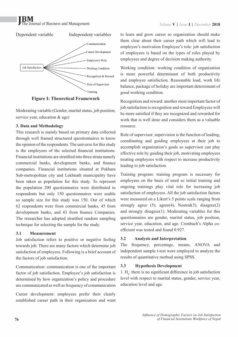
JBMVolume V | Issue I | December 2018The Journal of Business and Management
76
Dependent variable Independent variables
Figure I: Theoretical Framework
Moderating variable (Gender, marital status, job position, service year, education & age)
3. Data and MethodologyThis research is mainly based on primary data collected through well framed structured questionnaires to know the opinion of the respondents. The universe for this study is the employees of the selected financial institutions. Financial institutions are stratified into three strata namely commercial banks, development banks, and finance companies. Financial institutions situated at Pokhara Sub-metropolitan city and Lekhnath municipality have been taken as population for this study. To represent the population 200 questionnaires were distributed to respondents but only 150 questionnaires were usable so sample size for this study was 150. Out of which 62 respondents were from commercial banks, 45 from development banks, and 43 from finance Companies. The researcher has adopted stratified random sampling technique for selecting the sample for the study.
3.1 MeasurementJob satisfaction refers to positive or negative feeling towards job. There are many factors which determine job satisfaction of employees. Following is a brief account of the factors of job satisfaction.
Communication: communication is one of the important factor of job satisfaction. Employee’s job satisfaction is determined by how organization’s policy and procedure are communicated as well as frequency of communication
Career development: employees prefer their clearly established career path in their organization and want
to learn and grow career so organization should make them clear about their career path which will lead to employee’s motivation Employee’s role: job satisfaction of employees is based on the types of roles played by employees and degree of decision making authority.
Working condition: working condition of organization is more powerful determinant of both productivity and employee satisfaction. Reasonable load, work life balance, package of holiday are important determinant of good working condition.
Recognition and reward: another most important factor of job satisfaction is recognition and reward Employees will be more satisfied if they are recognized and rewarded for work that is well done and considers them as a valuable resource.
Role of supervisor: supervision is the function of leading, coordinating and guiding employees at their job to accomplish organization’s goals so supervisor can play effective role by guiding their job, motivating employees treating employees with respect to increase productivity leading to job satisfaction.
Training program: training program is necessary for employees on the basis of need so initial training and ongoing trainings play vital role for increasing job satisfaction of employees. All the job satisfaction factors were measured on a Likert’s 5 points scale ranging from strongly agree (5), agree(4), Neutral(3), disagree(2) and strongly disagree(1). Moderating variables for this questionnaires are gender, marital status, job position, service year, education, and age. Cronbach’s Alpha co-efficient was tested and found 0.927.
3.2 Analysis and InterpretationThe frequency, percentage, means, ANOVA and independent sample t-test were employed to analyze the results of quantitative method using SPSS.
3.3 Hypothesis Development1. H0: there is no significant difference in job satisfaction level with respect to marital status, gender, service year, education level and age.
Influence of Demographic Factors on Job Satisfaction of Financial Institutions Workforce of Nepal

JBMVolume V | Issue I | December 2018The Journal of Business and Management
77
4. Empirical Analysis
Table I: Social-demographic Profiles of Respondents
Personality Respon-dent
Percentage(%)
GenderMale 89 59.33
Female 61 40.67Total 150 100
MaritalStatus
Married 81 54Single 69 46
Divorced 0 0Widow 0 0Total 150 100
Job Position
Assistant 92 61.33Officer 30 20
Sr. officer 13 8.67Manager 15 10
Total 150 100
Service Year
Less than one 12 81-3 69 464-8 56 37.339-15 13 8.67
Over 15 0 0Total 150 100
Education
+2 Level 5 3.33Bachelor 50 33.33Masters 95 63.33M. Phil 0 0
Doctorate 0 0Total 150 100
Age
Under 20 1 0.6720-25 45 3026-30 69 4631-35 20 13.33
Over 35 15 10Total 150 100
With regard to the number of employees from different Nepalese financial institutions, the result showed that 62 from commercial bank, 45 from development bank, and 43 from financial institutions.
The highest percentage of respondents in Nepalese financial Institutions was male with 59.33 percent as compare to female with 40.67. With regard to marital status of respondents, the result showed that married respondent with highest percentage at 54 whereas single were at 46 percent.
With regard to job position the result showed that assistant with highest percentage at 61.33 percent as compare to officer with 20 percent, senior officer with 8.67 percent, and manager with 10 percent.
Regarding the year of service of respondents in the organization, most of the respondents were 1-3 years at 46 percent, whereas 4-8 years at 37.33 percent, 9-15 years at 8.67 percent, less than one year at 8 percent
Regarding the educational level of respondents, result showed that masters with highest percentage at 63.33 percent, whereas bachelor with 33.33 percent, and +2 levels with 3.33 percent.
Regarding the age group of respondents, result showed that respondents were mostly between 26-30 years with 46 percent, 20- 25 years with 30 percent, 31-35 with 13.33 percent, over 35 years with 10 percent and under 20 years with 0.67 percent.
Table II: Demographic Factors and Variables of Job Satisfaction
JobSatisfaction
Socio-Demographic FactorsVariables Gender
(p value)Marital status
(p value)Job position
(p value)Service Year
(p value) Education
(p value)Age
(p value)1 Communication .079* .539 .001*** .065* .740 .001***
2 Careerdevelopment .728 .597 .019** .234 .660 .050**
3 Employee’s role .008* .803 .001*** .376 .424 .038**
4 Working condition .306 .694 .106 .892 .976 .245
5 Recognition andreward .027** .886 .002*** .084* .863 .004***
6 Role of supervisor .339 .497 .096* .480 .609 .1127 Training .236 .729 .168 .317 .224 .062
*, ** &*** means the statistics is significant at 10%, 5% and 1% level of significance respectively.
Influence of Demographic Factors on Job Satisfaction of Financial Institutions Workforce of Nepal

JBMVolume V | Issue I | December 2018The Journal of Business and Management
78
ANOVA analysis shows that there is significant difference in the career development of employees with respect to job position and age of employees at 0.05 level. But there is no significant difference in the career development with respect to service year and education of employees, marital status and gender.
T-test shows that there is no significant difference in the career development with respect to gender and marital status of employees.
T-test shows that there is significant difference in the role of employees with respect to gender at 0.1 level but no significant difference with respect to marital status of employees. ANOVA analysis shows that there is significant difference in the role of employees with respect to job position and age of employees at 0.001, and 0.05 level respectively but no significant difference with respect to years of service and education of employees.
T-test and ANOVA analysis show that there is significant difference in working condition with respect to gender, marital status, job position, service year, education, and age of employee.
T-test shows that there is significant difference in recognition of employee and reward system of organization with respect to gender at 0.05 level but no significant difference with respect to marital status of employees. ANOVA analysis shows that there is significant difference in recognition and reward with respect to job position, service year, and age of employee at 0.05, 0.1, and 0.001 level respectively but no significant difference with respect to education of employees.
T-test shows that there is no significant difference in role of supervisor with respect gender and marital status of employee. ANOVA analysis shows that there is significant difference in role of supervisor with respect to job position at 0.1 level but no significant difference with respect to service year, education, and age of employees.
T-test shows that there is no significant difference in training program with respect to gender and marital status of employees. ANOVA analysis shows that there is significant difference in training program with respect to age at 0.1 level but no significant difference with respect to job positon, service year, and education of employees.
Table III: Demographic Factors and Level of Job Satisfaction
S.N. Variables t-value p-value
1 Gender and jobsatisfaction t=1.997 .048*
2 Marital status and jobsatisfaction t=.249 .769
3 Job position and jobsatisfaction F=5.566 .001**
4 Service year and jobsatisfaction F=1.614 .189
5 Education and jobsatisfaction F=.208 .813
6 Age and job satisfaction F=4.615 .002**
*&** means the statistics is significant at 5% and 1% level of significance respectively.
Table III revealed that there is significant difference in the level of job satisfaction with respect to male and female employees at 0.05 level. It is evident that gender influences the level of satisfaction of the respondents. So hypothesis set for this research has been rejected. In case of marital status there is no significant difference in the level of job satisfaction with respect to married and unmarried employees. So hypothesis set for marital status has been accepted and this finding is not supported by Ranjit (2012).
The ANOVA value (F=5.556) shows that there is significance difference in the level of job satisfaction with respect to job position of employees at 0.001 level. It is inferred that higher the position higher is the level of job satisfaction and vice versa. The hypothesis set for job position has been rejected.
The ANOVA analysis showed that there is no significant difference in the level of job satisfaction among the employees with respect to years of service(p>0.05). The finding shows that years of service of employees does not influence the level of job satisfaction. The hypothesis set for service years has been accepted and this finding is not supported by Ranjit (2012).
The ANOVA analysis showed that there is no significant difference in the level of job satisfaction with respect to education level of employees(p>0.05). The hypothesis set for level of education of employees has been accepted and this finding indicates that level of education does not influence the level of job satisfaction of employees.
Influence of Demographic Factors on Job Satisfaction of Financial Institutions Workforce of Nepal

JBMVolume V | Issue I | December 2018The Journal of Business and Management
79Influence of Demographic Factors on Job Satisfaction of Financial Institutions Workforce of Nepal
However this finding is not supported by Ranjit, (2012) & Sukumar (2009).
The ANOVA analysis showed that there is significant difference between age of employees and level of job satisfaction at 0.01 level. It is concluded that higher the age higher is the level of job satisfaction. This finding is supported by Ranjit (2012), Tom, & Smith (2007).
5. ConclusionThe result revealed the influence of demographic variable (gender, marital status, job position, service years, education, and age) on job satisfaction of employees of Nepalese financial institutions. Communication, career development, role of employee, working condition, recognition and reward, role of supervisor, and training program have been taken as independent variables. In
banking sector in Nepal, gender, job position, service year, age of employees do influence on communication pattern of organizational communication whereas marital status, education do not have any influences. Job position, and age of employees have influence on career development whereas gender, marital status service year, education do not have any influences. Gender, job position, and age of employees have influences but marital status, service year and education do not have any influence. The result revealed that, job position, and age of employees influence the level of job satisfaction in Nepalese financial institutions. This study also reveals that there is no influence of years of service, level of education, and marital status of employees on level of job satisfaction.
References
Adhikari, D.R, & Gautam, D.K. (2011). Employees’ commitment and organizational performance in Nepal: A typology framework. SEBON Journal, 2, 1-17.
Beisiegel, H., (2003). Diversity builds strength.Productivity, 19(2), 26.
Bhati, P. P., & Ashok, M. (2013). Study relationship between demographic variables and job satisfaction of employee of ceramic industry. Global Reserch Analysis International, 2(9), 114-116.
Cetin, M. O. (2006). The relationship between Job Satisfaction, Occupation and Organization Commitment. Academy of Business Journal, 8(1), 78-90.
Daftuar, C. N. (2001). Job satisfaction among government officers: A comparison of three m e a s u r e s . Abhigyan, 19(3), 33 – 39.
Din, S.U., Zaman, K.U & Nawas, A. (2010). Impacts of demographic variables on job satisfaction o f the academicians in University of NWFP. Pakistan Bulletin of Education & Research, 32(1), 53-58.
Ellickson, M., & Logsdon, K. (2001). Determinants of job satisfaction of municipal government employees. State and Local Government Review, 33(3), 173-84.
Katuwal, S. B., & Randhawa, G. (2007). A study of job satisfaction of public & private sector Nepalese textile workers. Indian Journal of Industrial Relations, 43(2), 15-31.
Mosadeghrad, A. M., Ferlie, E., & Rosenberg, D. (2008). A study of the relationship between job satisfaction, organizational commitment and turnover intention among hospital employees. Health Services Management Research, 21(4), 211-227.
Orisatoki, R. O., & Oguntibeju O.O. (2010). Job satisfaction among selected workers in St Lucia, West Indies. Scientific Research and Essays, 5(12), 1436-1441.
Ranjit, L. (2012). Study on influence of demographic factors on job satisfaction of textile mill - workers. Zenith International Journal of Business Economics & Management Research, 2, 14-29.
Tabatabaci, S., Ghaneh, S., Mohaddes, H., & Khansani, M. (2013). Relationship of job satisfaction and demographic variables in Pars Ceram factory. Social and Behavioral Science, 84, 17 9 5 - 1 8 0 0 . Doi: 10:1016/j.sbspro.07.036.
JBMVolume V | Issue I | December 2018The Journal of Business and Management
80
The Semiotics of Contemporary Visual Texts: A Study in New Rhetorical Analysis
Bishwo Raj Parajuli1
AbstractThis paper explores the semiotics of selected typical visual texts of our time and their implicatures. Some theoretical and conceptual tools for textual interpretation with regards to textual elements exist. However, contemporary visual texts are still prospective area of study. Considering such gap, I have chosen the visual texts that we encounter in our day to day and professional life. For delimitation purposes, only three types of visual communication events have been discussed, selected brochures of academic institutions, selected printed advertisements, and selected billboard advertisements. The analytical tools are predominantly critical discourse of the various motifs, images, structures and persuasive strategies used in the texts. The basic architecture of the discussion part is based on thick descriptions of the textual contents highlighting the semiotics of each. Findings of the study focus on semiotic implications and connotations of the key rhetorical elements. The major finding of the study is most of the visual texts principally try to glorify, glamorize and even exoticize the product or service. The conclusion derived is nothing like absolute conclusion. It is just an array of possible interpretations that pave path for a new discourse like– should we take them for granted? All in all, this is a new rhetorical analysis by outlook.
Keywords: New Rhetorical Analysis, Semiotics, Visual Texts,
1. IntroductionSemiotics is the study of sign system in popular arts and other contemporary forms of communication. This practice has taken the firmest hold in approaches to any form of popular culture like movies, television programmes, women’s magazine and tabloids, billboard and printed ads and so on (Green& Lebihan, 2011).
Since the sign systems in semiotics are non-linguistic, they demand special cross-cultural understanding of different walks of life, paralinguistic clues and cues, and an array of visual language among many others. For instance, if a boss wants to cut off his manual work force through automation technology, the technology or medium of change itself can be a powerful message.
A prominent media analyst Marshall McLuhan states that disproportionate use of technology and automation technology in twentieth and twenty first century is not just an indicator of development, this tendency is leading
us towards a menacing age of mechanization. We are bound to destroy the role of human work force and human association in works. In the words of McLuhan, “…it was not the machine, but what one did with the machine, that was its meaning or message (2000)” This is exactly the point where comparatively novel and pragmatic subjects like technical communication are interested.
Practically technical communication activities have been running through ages, probably beginning with the morn of human civilization. The primitive frescos and hieroglyphics for some kind of coded information are ancient form of technical communication activities. Similarly, Aayurvedas, Manusmriti (The Laws of sage Manu), and architectural designs of our ancestors like Araniko etc are other examples our ancient technical communication texts (Adhikari & Upadhyaya, 2014). So much so that even current medical prescriptions of the physicians are also a kind of technical communication.
1 Lecturer, School of Business, Pokhara University
ISSN 2350-8868

JBMVolume V | Issue I | December 2018The Journal of Business and Management
81The Semiotics of Contemporary Visual Texts: A Study in New Rhetorical Analysis
Thanks to illegible handwritings of doctors, we do not have to bother to decode their sign systems; only the pharmacists can read them.
Communication theorists Gerson and Gerson opine that technical communication is oral and written communication for and about business and industry. It focuses on communicating about products and services- how to manufacture them, market then, deliver them, and use them (Gerson and Gerson, 2014).
In this context, one of the interesting questions that trigger our mind is: how do the manufactures design to communicate through a subtle semiotic system? And what are the implications and objectives of such semiotic system? This research paper deals with typical events of technical communication and study implicatures of the major signs (as codes of visual communication) from a new rhetorical analysis point of view.
2. Data and MethodologyThis paper tries to explicate some typical technical communication events focusing on some contemporary visual texts. For delimitation purposes, only three types of representative technical communication texts have been selected. They are representative in the sense that they appear more patternized, frequent, popular and communicative in the present context. So, methodologically, it is convenient sampling. Thick descriptions based on in-depth observation of the selected communication acts will be followed by content analysis. As a whole, the texts will be scrutinized from post structural outlook like new rhetorical analysis.
New Rhetorical Analysis : A Theoretical ReviewRhetorical analysis is a form of criticism with a long tradition shared by scholars from various disciplines. The general focus of rhetorical analysis is to arrive methodically at insights into the performance of a communication event (or assemblage of events) through an investigation of selected features of the event. Rhetorical analysis, therefore, offers scholars a principled approach to describe how communication works in a given instance.
I. Identify the text for analysis
II.Categorize the text according to purpose and type
III.Identify constiuent parts of texts
IV. Interpret and discuss on or more configuratios of the parts and / or whole of the text(s) in relationship with some overarching theoretical concepts
→ → →
Figure I: Basic Approach in Rhetorical Analysis
Rhetorical analysis focuses on the textual components and effects of those components on the perception of the person experiencing it.
There are three waves in rhetorical criticism: traditional, new rhetorical and critical post modern. However, the so-called new rhetorical and critical postmodern theorists climb upon the shoulder of classical theorist Aristotle and try to de- canonize the established ways of interpreting the structurally and strategically functioning constituents of texts.
Referring to Aristotle’s conception about rhetoric, Mark Zachry defines: rhetoric is the use of artful language based means to affect belief. Individuals persuade others through three means: the character or credibility of the source of information (ethos), the stirring of emotions in the individual being persuaded (pathos) and proof of truth through reasonable arguments (logos). Theoretically, these three means of persuasion are popularly known as rhetorical appeals.
Aristotle has also offered classical approaches of rhetorical performance. Rhetoric can be deliberative, forensic and demonstrative or epideictic (2009, p.71).
Deliberative rhetorical performances are concerned with questions like what should be done is a given situation or deciding future courses of actions.
Forensic approach focuses on establishing what is just and unjust through judicial deliberations about things. And, demonstrative or epideictic form of rhetoric is concerned with demonstrating or establishing the merits of something for the public.
In the first half of twentieth century, rhetorical criticism as such was de-canonized as communication got more
JBMVolume V | Issue I | December 2018The Journal of Business and Management
82
complex due to the advancement in industry, science, technology and complicated human relationship. Due to such insights, some theorists considered it as New Rhetorical criticism. This approach is rather a post structural school of criticism rather than individual promulgation of a theorist.
In the second half of twentieth century and throughout twenty first century, almost every walk of human life has been guided by post modern thoughts-obviously including rhetorical criticism. Especially, deconstructionist view believes that meaning is possible only because of privileged use of language and its arbitrary system that guides us to perceive things according to some logo-centric symbolization. Thus, a deconstructionist reading of a text subverts its apparent significance by uncovering contradictions and conflicts within it.
In this paper, rather than interpreting a text or act of communication from structural or formulaic perspectives, we shall create an array of meanings for critiquing purpose and look at them from new rhetorical perspective. For discussion purpose only, selected printed visual texts which can be typically labeled as technical communication, have been presented below.
3. Discussion of the Selected Studies
Study 1: Tertiary level brochures
Now-a-days, it is fashionable as well as ritualistic for academic institutions, especially tertiary and university level colleges to print attractive brochures in glossy booklet forms. Perhaps this is due to the influence of commodification ideology. It is a tell-tale fact that institutions and organizations are judged even on the basis of glamour and quality of the brochure. Just like glamour tabloids and magazines, these publications also aim to glamorize and glorify their selling points.
The masterminds of these texts seem to be interested to glamorize good looking students. A good look of face and anatomy is always a hot selling commodity for fast-growing consumerism. Business houses and industrialist understand this fact very well. So, it is quite common and expected tendency that people from fashion industry and mass media use (and even exploit) skinny and sensuous
models and celebrities to advertise their products. In the present context, education has become mother business of all other businesses. Following the footsteps of other business people, educationists are also using beauty and fanciful presentation of college teenagers in their prospectus.
This tendency was identified after a thorough study of selected brochures over a couple of years (See Exhibit 1, Appendix). Then the focal images were sorted into four groups- images of female student models, images of male student models, mixed images and others. Majority of the images were that of girl students. Almost all the major images in these brochure pages are restricted to three Bs coined as ‘Bold, Big and Beautiful’ by Kaul (2014).
Study 2: Print ads cuts
This is the age of media. Especially popular mass media like social networking sites (facebook, instagram etc.), radio, television programmes, music videos, cinemas, daily newspapers, glamour tabloids, etc. have created a vibe in modern generation and they are considerably successful in brainwashing the mindset of consumers through visual appeals created by human anatomy and face. Especially, print media is notorious in creating media blitz by glamorizing the commonplace and changing it into paramount. In terms of model selection, these advertisements pay more attention to stereotyped images and gender roles. For instance, their first priority is upon fair complexioned skinny models, beautiful housewives. At the bottom of their list is a gentleman with a common apparition. Their basic motive is glorification of the commodities through celebrity endorsement and sensuous models. In other words, plump, short of height, dark skinned or anyone with deformity (as the majority of people think) would hardly fit as models in these cases.
Study3: Billboard ads
Billboard advertisements are not very much different from print advertisements and college brochures. A typical formula or motif in billboard is using a colossal image of a celebrity model (preferably a female) as focal image and placing it somewhere where majority of the public
The Semiotics of Contemporary Visual Texts: A Study in New Rhetorical Analysis
JBMVolume V | Issue I | December 2018The Journal of Business and Management
83The Semiotics of Contemporary Visual Texts: A Study in New Rhetorical Analysis
can have eye contact. It is an attempt of looming over onlookers’ visual selection. Furthermore, in the words of Rutherford, photographs do not necessarily indicate size; some photographs show the objects (referring to the models) next to something common. This is also known as technique of juxtaposition and amplification (Rutherford 2006). Recently, full page photograph of an acclaimed political leader in Nepal was published in most of the national newspapers (See Exhibit 3 in Appendix) and huge billboards in different parts of the city. This unusually celebrated coverage of an acclaimed political leader throughout the media houses and entry points of the town was not a common phenomenon. It was an attempt of stereotyping a celebrated political leader as a hero. The way the leader was projected as a hero or messiah of nation building was questioned by many skeptics. However, from communication point of view, this gigantic projection of a leader who emerged from grassroots level is something like McLuhan’s maxim– ‘Medium is the message’. To rephrase it in a better coinage of McLuhan, it is a hot medium. According to McLuhan, “A hot medium is one that extends one single sense in high definition. High definition is the state to being well filled with data. A photograph is visually high definition (2000, p.30).” So this particular publicity of a political leader is a good example of how media can be used as hot or cold to influence the perceptions of audience.
Furthermore, the billboard or even printed advertisements as such are full of semiotic implications. In the eyes of semioticians, they underlie distinct myths and their structural connotation is distinct. Either they follow social norms or violate social norms. According to the structural analyst John Fiske– “…widely accepted conventions are close to the norms. The unexpected, the non conventional is a deviation from the norm” (1990, p. 101). For example, in Exhibit 3, the halo behind the head of the leader and the semiotics of red color scheme are connotative of the non conventional and deviation from the norm. In other words, it is an attempt of creating a myth of a revolutionary hero.
4. ConclusionLanguage is ineffable means to express human emotions
and feelings despite its pivotal role in successful communication. A visual language is more expressive than written scripts or verbal mode of communication. The verbal mode of communication, i.e. language, has its own limitations. After all language can not express everything we want to convey. What we aim to convey gets conveyed more nonverbally than verbally. So the designers of the discussed communication events have focused on using non-verbal signs of mass persuasion to attract the audience. In general following tendencies can be observed in these texts:The patterns and configuration of the matters are important in the act of communication. They reflect culture and quality through pictures, archives, location and statistics. Even paper and printing quality can not be ignored; After all, medium is the message. However, credibility and acceptability of the asserted messages are always questionable.
� Mostly these texts focus less on written contents. Major focus is given to visual and graphical appeal. Their basic motive is to loom over the visual selection of the onlookers through sensuous appeal. Only a few of them are able to create aesthetical appeal.
� There are attempts to project charisma in the model; and these charismatic projections happen in stereotyped forms. For instance, they have used a traditional concept of a hero or a model.
� Using McLuhan’s terminologies, these texts of technical communication are rich in hot medium of message. However, in Aristotelian rhetorical paradigm, one would grade them as poor in ethos, pathos and logos. Moreover, they are less forensic, slightly deliberative and more demonstrative in nature.
� These pieces aim to create some structural myths such as- A leader as a hero, a model or celebrity as a true brand ambassador of the products in their hands, girls or good looking students as the messenger of success and so on. All these semiotics and stereotyped concepts can be critically examined from New rhetorical point of view.

JBMVolume V | Issue I | December 2018The Journal of Business and Management
84
Adhikari, D. & Upadhyaya, .(2014), Technical Communication. Kathmandu: Buddha Publications.
Fiske, J. (1990). Introduction to Communication Studies. New Delhi:Routledge.
Gerson, S. & Gerson, S. (2014). Communication: Process & Product. New Delhi: Pearson.
Green, K. & Lebihan, J. (2011). Critical theory & practices. New Delhi: Routledge.
Kaul, A. (2014). Business Communication. Delhi: PHI.
Lois, T. ( 2006) Critical Theory Today. Routledge: India.
McLuhan, M. (2000). Understanding Media. Media Studies. CDE, TU: Kathmandu.
Rutherford, Andrea J. (2006). Basic Communication Skills for Technology. Pearson India.
Zachry, M. (2009). Rhetorical Analysis. The Handbook of Business Discourse (ed. by Chiappini, Francesca B.) Edinburgh: Edinburgh University Press.
References
Appendix
Exhibit 1
Exhibit 2 Exhibit 3
The Semiotics of Contemporary Visual Texts: A Study in New Rhetorical Analysis