ITO FORMULAS FOR FRACTIONAL BROWNIAN

MOTIONS

Robert J. Elliott

Haskayne School of Business, University of Calgary

1

ABSTRACT

The difficulty of studying financial models with fractional Brow-

nian motions is partly due to the fact that the stochastic calculus

for fractional Brownian motions is not as well developed as for

traditional models. Ito formulas play an important role in this

stochastic calculus. This paper will review the current state of

knowledge of such formulas and present a new and transparent

approach to the derivation of these generalized Ito formulas. We

will present applications to financial models. This presentation

represents joint work with John van der Hoek from the Univer-

sity of Adelaide.

2

What is FBM ?

For each Hurst index 0 < H < 1

BH =BH(t), t ∈ R

is a Gaussian process with mean 0 for each t and covariance

E[BH(t)BH(s)

]=

1

2

[|t|2H + |s|2H − |t− s|2H

]We now take BH(0) = 0, B

12 is a standard Brownian motion.

E[(BH(t) −BH(s)

)2]= |t− s|2H

defined on a suitable probability space (Ω,F , P ), with expectationoperator E[·]

3

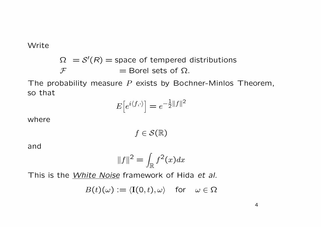
Write

Ω = S′(R) = space of tempered distributions

F = Borel sets of Ω.

The probability measure P exists by Bochner-Minlos Theorem,so that

E[ei〈f,·〉

]= e−

12‖f‖2

where

f ∈ S(R)

and

‖f‖2 =∫R

f2(x)dx

This is the White Noise framework of Hida et al.

B(t)(ω) := 〈I(0, t), ω〉 for ω ∈ Ω

4

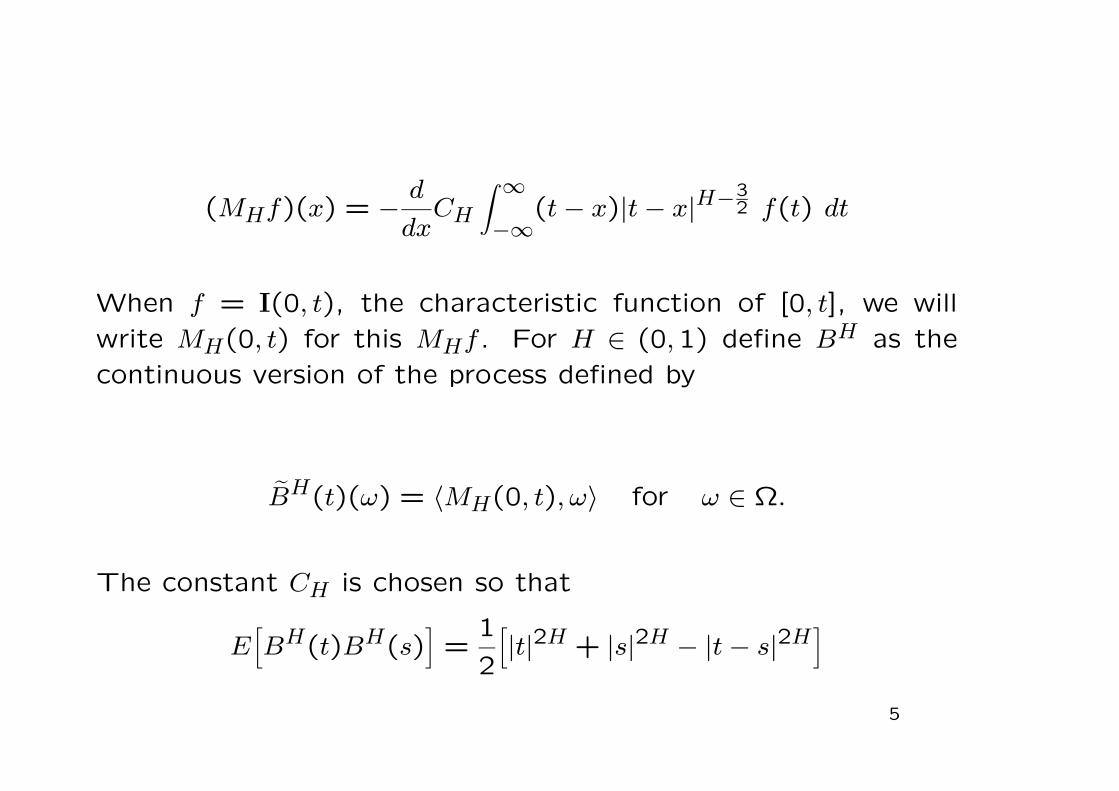
(MHf)(x) = − d

dxCH

∫ ∞−∞

(t− x)|t− x|H−32 f(t) dt

When f = I(0, t), the characteristic function of [0, t], we will

write MH(0, t) for this MHf . For H ∈ (0,1) define BH as the

continuous version of the process defined by

BH(t)(ω) = 〈MH(0, t), ω〉 for ω ∈ Ω.

The constant CH is chosen so that

E[BH(t)BH(s)

]=

1

2

[|t|2H + |s|2H − |t− s|2H

]5

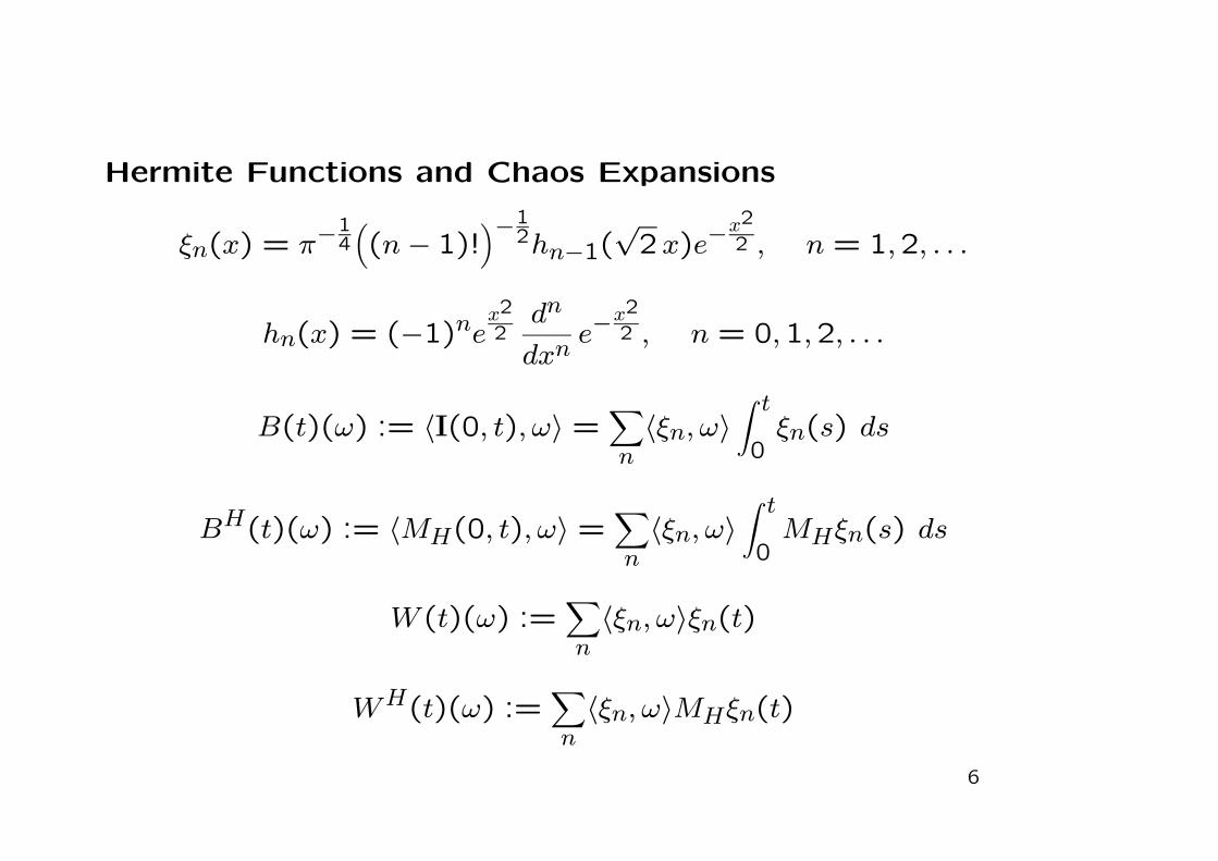
Hermite Functions and Chaos Expansions

ξn(x) = π−14((n− 1)!

)−12hn−1(

√2x)e−

x22 , n = 1,2, . . .

hn(x) = (−1)nex22dn

dxne−

x22 , n = 0,1,2, . . .

B(t)(ω) := 〈I(0, t), ω〉 =∑n〈ξn, ω〉

∫ t

0ξn(s) ds

BH(t)(ω) := 〈MH(0, t), ω〉 =∑n〈ξn, ω〉

∫ t

0MHξn(s) ds

W (t)(ω) :=∑n〈ξn, ω〉ξn(t)

WH(t)(ω) :=∑n〈ξn, ω〉MHξn(t)

6

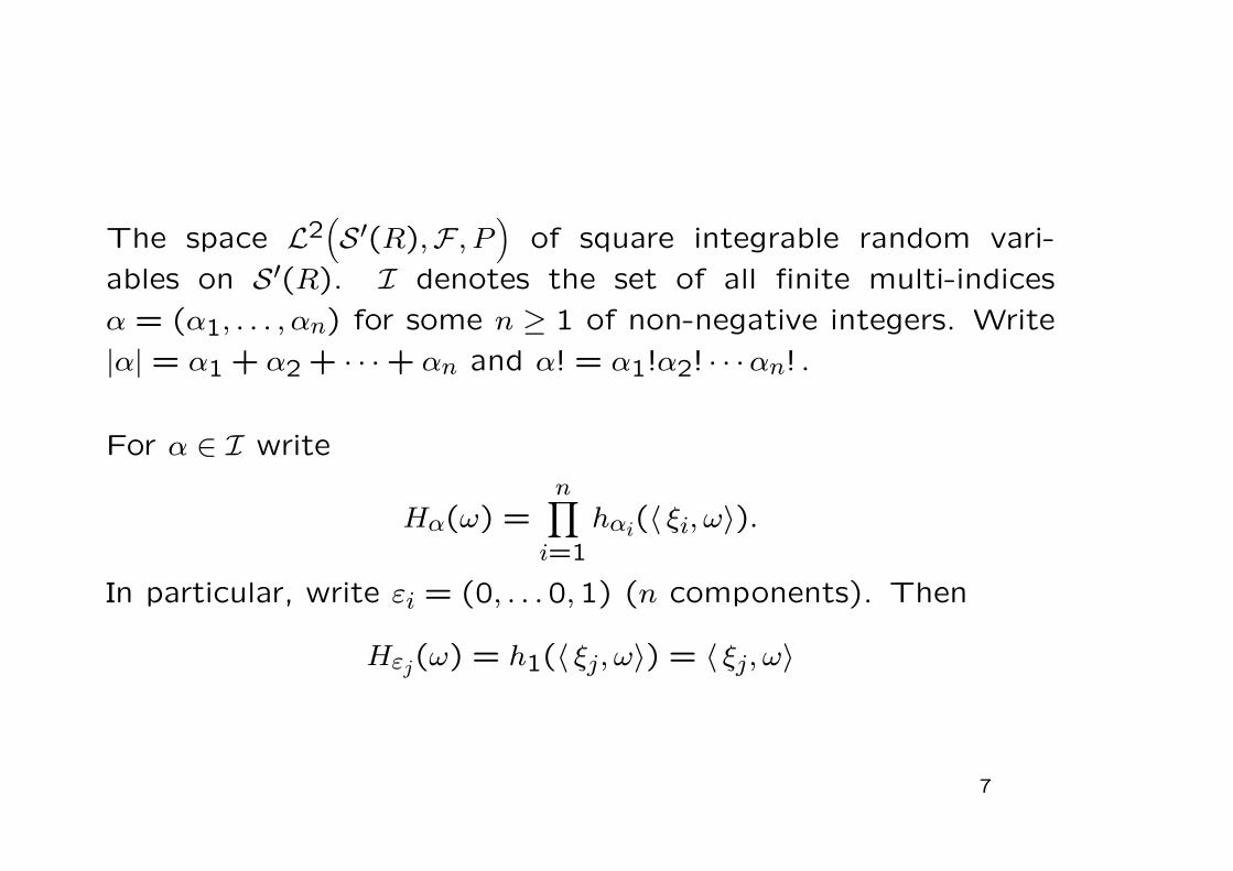
The space L2(S′(R),F , P

)of square integrable random vari-

ables on S′(R). I denotes the set of all finite multi-indices

α = (α1, . . . , αn) for some n ≥ 1 of non-negative integers. Write

|α| = α1 + α2 + · · · + αn and α! = α1!α2! · · ·αn! .

For α ∈ I write

Hα(ω) =n∏i=1

hαi(〈 ξi, ω〉).

In particular, write εi = (0, . . .0,1) (n components). Then

Hεj(ω) = h1(〈 ξj, ω〉) = 〈 ξj, ω〉

7

Every F ∈ L2(S′(R),F , P

)has a unique representation

F (ω) =∑α∈I

cαHα(ω)

=∑αcαhα1(〈 ξ1, ω〉) . . . hαn(〈 ξn, ω〉)

and

E[HαHβ] = α!δα,β

‖F‖2 =∑α∈I

α!c2α

8

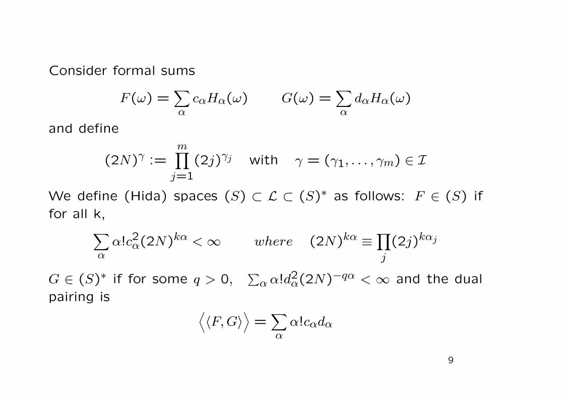
Consider formal sums

F (ω) =∑αcαHα(ω) G(ω) =

∑αdαHα(ω)

and define

(2N)γ :=m∏j=1

(2j)γj with γ = (γ1, . . . , γm) ∈ I

We define (Hida) spaces (S) ⊂ L ⊂ (S)∗ as follows: F ∈ (S) if

for all k,∑αα!c2α(2N)kα <∞ where (2N)kα ≡ ∏

j

(2j)kαj

G ∈ (S)∗ if for some q > 0,∑α α!d

2α(2N)−qα < ∞ and the dual

pairing is ⟨〈F,G〉

⟩=

∑αα!cαdα

9

Suppose Z : R → (S)∗ is such that⟨〈Z(t), F 〉

⟩∈ L1(R) for all

F ∈ (S)

Then∫RZ(t)dt is defined to be that unique element of (S)∗ such

that

⟨〈∫RZ(t)dt, F 〉

⟩=

∫R

⟨〈Z(t), F 〉

⟩dt for all F ∈ (S)

We then say that Z(t) is integrable in (S)∗

10

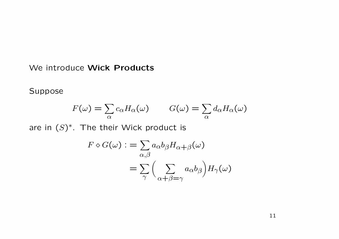
We introduce Wick Products

Suppose

F (ω) =∑αcαHα(ω) G(ω) =

∑αdαHα(ω)

are in (S)∗. The their Wick product is

F G(ω) : =∑α,β

aαbβHα+β(ω)

=∑γ

( ∑α+β=γ

aαbβ

)Hγ(ω)

11

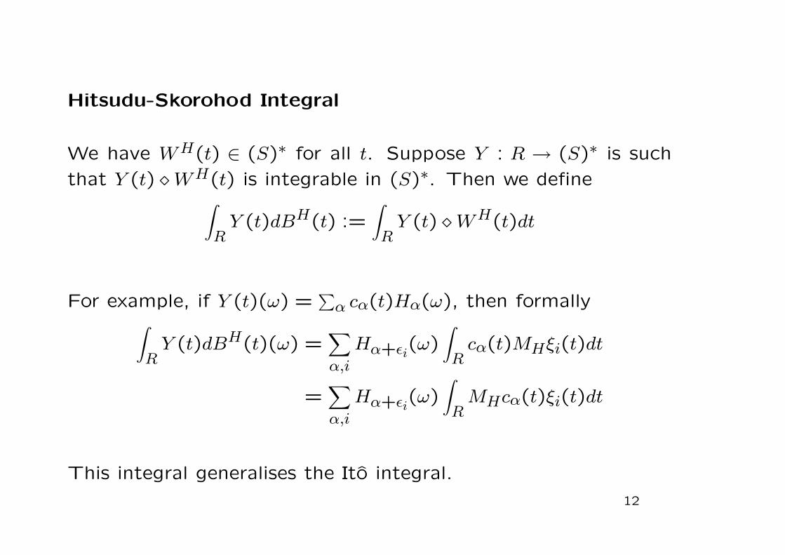
Hitsudu-Skorohod Integral

We have WH(t) ∈ (S)∗ for all t. Suppose Y : R → (S)∗ is such

that Y (t) WH(t) is integrable in (S)∗. Then we define∫RY (t)dBH(t) :=

∫RY (t) WH(t)dt

For example, if Y (t)(ω) =∑α cα(t)Hα(ω), then formally∫

RY (t)dBH(t)(ω) =

∑α,i

Hα+εi(ω)∫Rcα(t)MHξi(t)dt

=∑α,i

Hα+εi(ω)∫RMHcα(t)ξi(t)dt

This integral generalises the Ito integral.

12

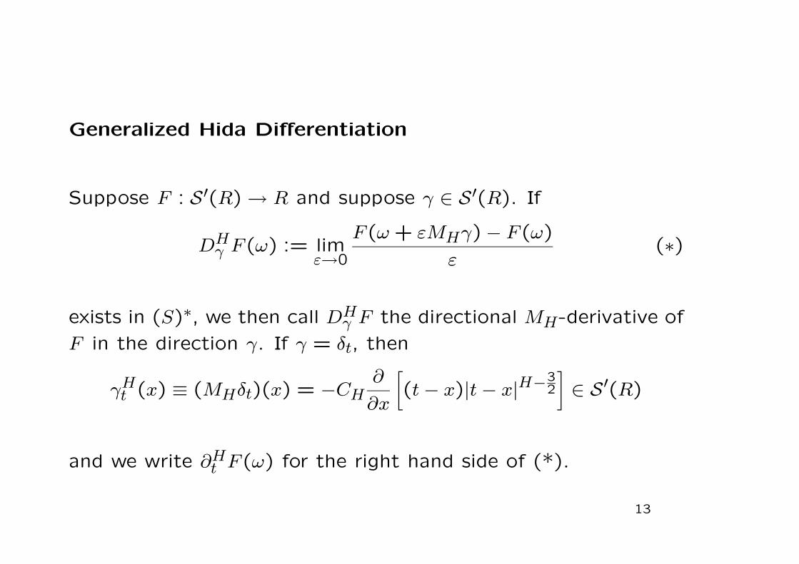
Generalized Hida Differentiation

Suppose F : S′(R) → R and suppose γ ∈ S′(R). If

DHγ F (ω) := lim

ε→0

F (ω+ εMHγ) − F (ω)

ε(∗)

exists in (S)∗, we then call DHγ F the directional MH-derivative of

F in the direction γ. If γ = δt, then

γHt (x) ≡ (MHδt)(x) = −CH∂

∂x

[(t− x)|t− x|H−3

2

]∈ S′(R)

and we write ∂Ht F (ω) for the right hand side of (*).

13

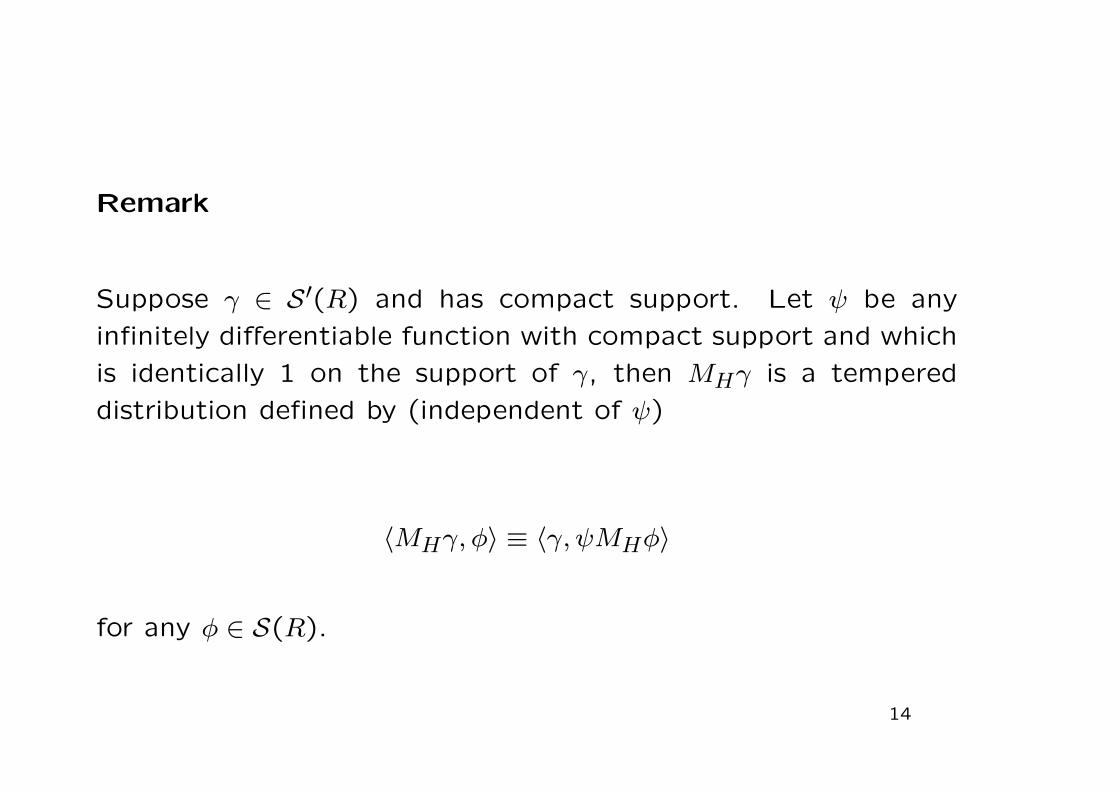
Remark

Suppose γ ∈ S′(R) and has compact support. Let ψ be any

infinitely differentiable function with compact support and which

is identically 1 on the support of γ, then MHγ is a tempered

distribution defined by (independent of ψ)

〈MHγ, φ〉 ≡ 〈γ, ψMHφ〉

for any φ ∈ S(R).

14

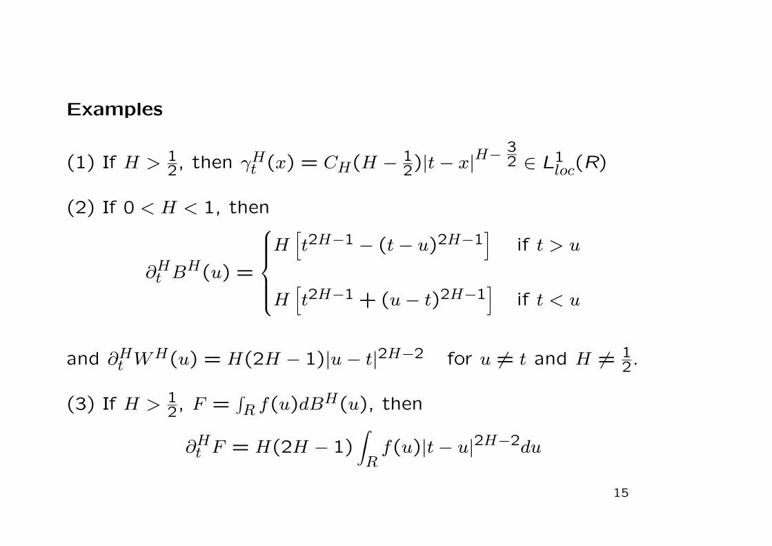
Examples

(1) If H > 12, then γHt (x) = CH(H − 1

2)|t− x|H− 32 ∈ L1

loc(R)

(2) If 0 < H < 1, then

∂Ht BH(u) =

⎧⎪⎪⎪⎨⎪⎪⎪⎩H

[t2H−1 − (t− u)2H−1

]if t > u

H[t2H−1 + (u− t)2H−1

]if t < u

and ∂Ht WH(u) = H(2H − 1)|u− t|2H−2 for u = t and H = 1

2.

(3) If H > 12, F =

∫R f(u)dB

H(u), then

∂Ht F = H(2H − 1)∫Rf(u)|t− u|2H−2du

15

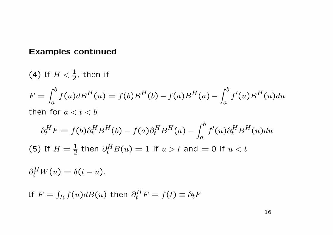
Examples continued

(4) If H < 12, then if

F =∫ b

af(u)dBH(u) = f(b)BH(b)− f(a)BH(a)−

∫ b

af ′(u)BH(u)du

then for a < t < b

∂Ht F = f(b)∂Ht BH(b) − f(a)∂Ht B

H(a) −∫ b

af ′(u)∂Ht BH(u)du

(5) If H = 12 then ∂Ht B(u) = 1 if u > t and = 0 if u < t

∂Ht W (u) = δ(t− u).

If F =∫R f(u)dB(u) then ∂Ht F = f(t) ≡ ∂tF

16

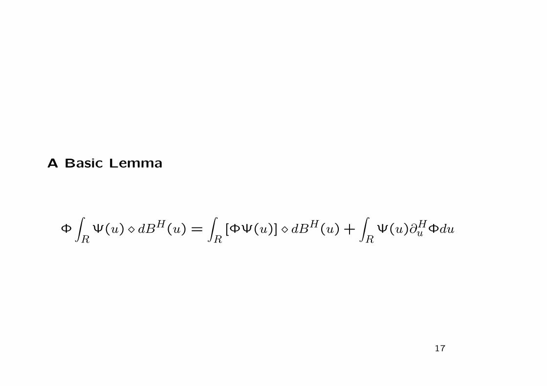
A Basic Lemma

Φ∫R

Ψ(u) dBH(u) =∫R

[ΦΨ(u)] dBH(u) +∫R

Ψ(u)∂Hu Φdu

17

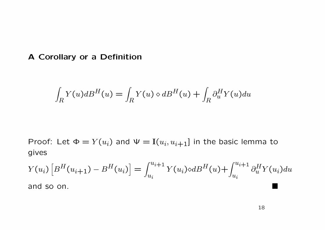
A Corollary or a Definition

∫RY (u)dBH(u) =

∫RY (u) dBH(u) +

∫R∂Hu Y (u)du

Proof: Let Φ = Y (ui) and Ψ = I(ui, ui+1] in the basic lemma to

gives

Y (ui)[BH(ui+1) −BH(ui)

]=

∫ ui+1

uiY (ui) dBH(u)+

∫ ui+1

ui∂Hu Y (ui)du

and so on.

18

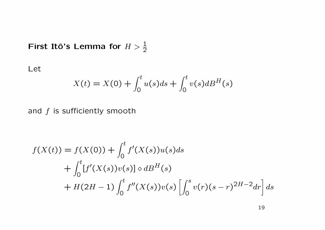
First Ito’s Lemma for H > 12

Let

X(t) = X(0) +∫ t

0u(s)ds+

∫ t

0v(s)dBH(s)

and f is sufficiently smooth

f(X(t)) = f(X(0)) +∫ t

0f ′(X(s))u(s)ds

+∫ t

0[f ′(X(s))v(s)] dBH(s)

+H(2H − 1)∫ t

0f ′′(X(s))v(s)

[∫ s

0v(r)(s− r)2H−2dr

]ds

19

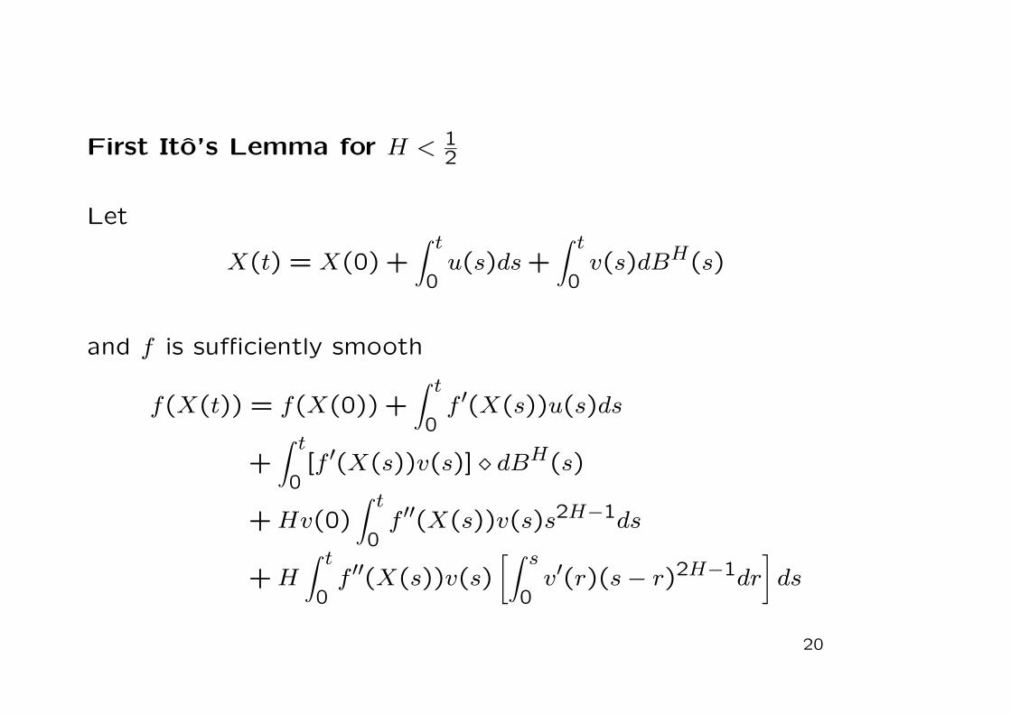
First Ito’s Lemma for H < 12

Let

X(t) = X(0) +∫ t

0u(s)ds+

∫ t

0v(s)dBH(s)

and f is sufficiently smooth

f(X(t)) = f(X(0)) +∫ t

0f ′(X(s))u(s)ds

+∫ t

0[f ′(X(s))v(s)] dBH(s)

+Hv(0)∫ t

0f ′′(X(s))v(s)s2H−1ds

+H∫ t

0f ′′(X(s))v(s)

[∫ s

0v′(r)(s− r)2H−1dr

]ds

20

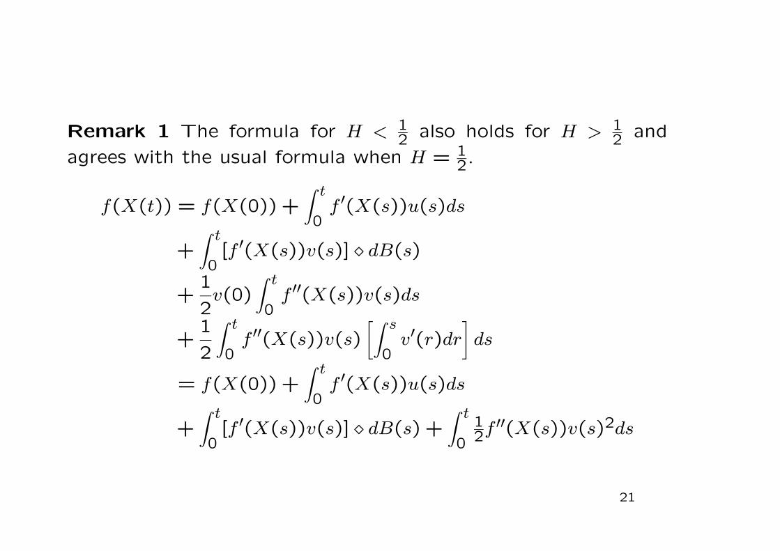
Remark 1 The formula for H < 12 also holds for H > 1

2 and

agrees with the usual formula when H = 12.

f(X(t)) = f(X(0)) +∫ t

0f ′(X(s))u(s)ds

+∫ t

0[f ′(X(s))v(s)] dB(s)

+1

2v(0)

∫ t

0f ′′(X(s))v(s)ds

+1

2

∫ t

0f ′′(X(s))v(s)

[∫ s

0v′(r)dr

]ds

= f(X(0)) +∫ t

0f ′(X(s))u(s)ds

+∫ t

0[f ′(X(s))v(s)] dB(s) +

∫ t

0

12f

′′(X(s))v(s)2ds

21

Remark 2

When X(t) = BH(t), it is now well known that

f(BH(t)) = f(0)+∫ t

0f ′(BH(s)) dBH(s)+H

∫ t

0f ′′(BH(s))s2H−1ds

which again agrees with the usual formula when H = 12.

22

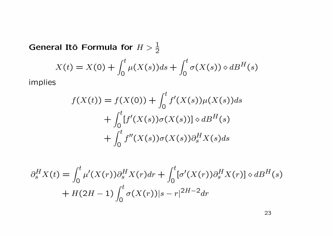
General Ito Formula for H > 12

X(t) = X(0) +∫ t

0µ(X(s))ds+

∫ t

0σ(X(s)) dBH(s)

implies

f(X(t)) = f(X(0)) +∫ t

0f ′(X(s))µ(X(s))ds

+∫ t

0[f ′(X(s))σ(X(s))] dBH(s)

+∫ t

0f ′′(X(s))σ(X(s))∂Hs X(s)ds

∂Hs X(t) =∫ t

0µ′(X(r))∂Hs X(r)dr+

∫ t

0[σ′(X(r))∂Hs X(r)] dBH(s)

+H(2H − 1)∫ t

0σ(X(r))|s− r|2H−2dr

23

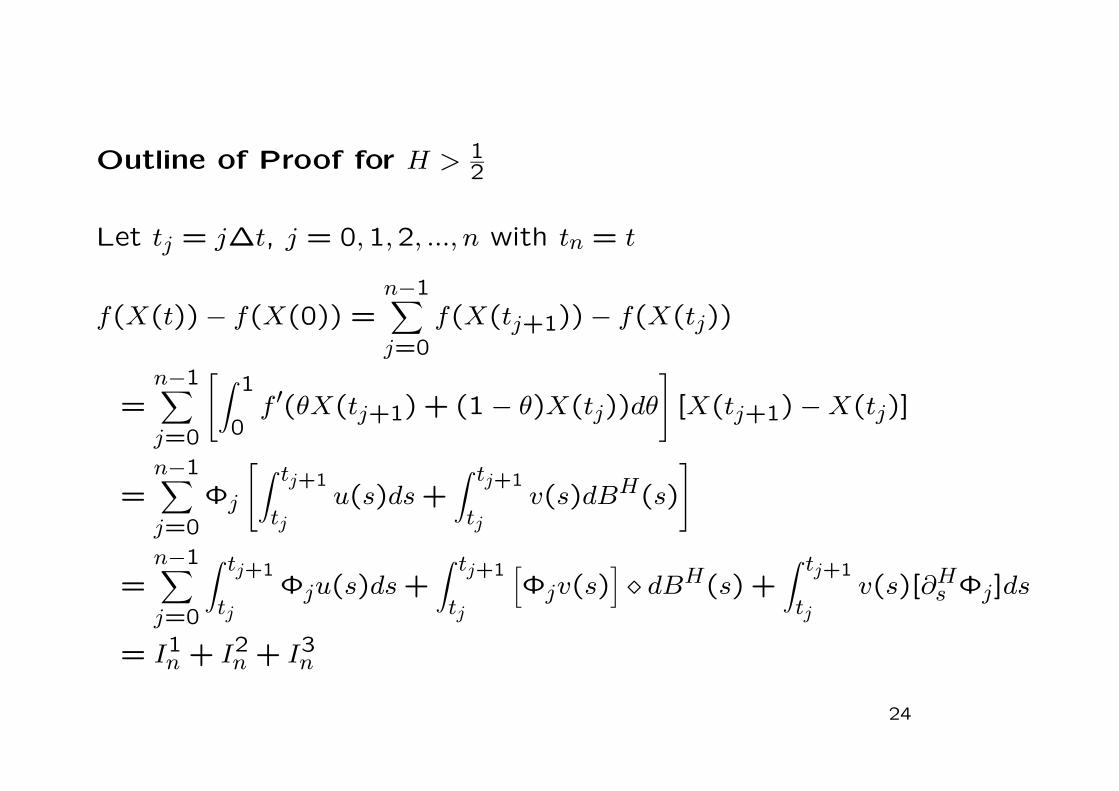
Outline of Proof for H > 12

Let tj = j∆t, j = 0,1,2, ..., n with tn = t

f(X(t)) − f(X(0)) =n−1∑j=0

f(X(tj+1)) − f(X(tj))

=n−1∑j=0

[∫ 1

0f ′(θX(tj+1) + (1 − θ)X(tj))dθ

][X(tj+1) −X(tj)]

=n−1∑j=0

Φj

[∫ tj+1

tju(s)ds+

∫ tj+1

tjv(s)dBH(s)

]

=n−1∑j=0

∫ tj+1

tjΦju(s)ds+

∫ tj+1

tj

[Φjv(s)

] dBH(s) +

∫ tj+1

tjv(s)[∂Hs Φj]ds

= I1n + I2n + I3n

24

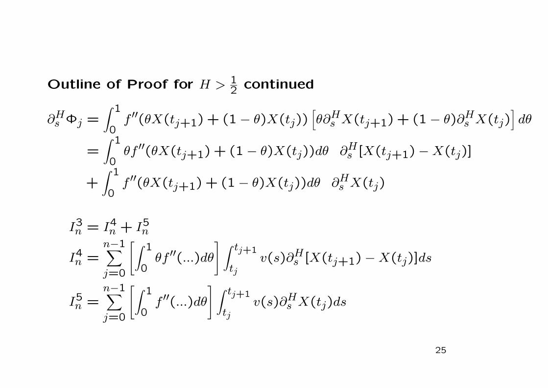
Outline of Proof for H > 12 continued

∂Hs Φj =∫ 1

0f ′′(θX(tj+1) + (1 − θ)X(tj))

[θ∂Hs X(tj+1) + (1 − θ)∂Hs X(tj)

]dθ

=∫ 1

0θf ′′(θX(tj+1) + (1 − θ)X(tj))dθ ∂Hs [X(tj+1) −X(tj)]

+∫ 1

0f ′′(θX(tj+1) + (1 − θ)X(tj))dθ ∂Hs X(tj)

I3n = I4n + I5n

I4n =n−1∑j=0

[∫ 1

0θf ′′(...)dθ

] ∫ tj+1

tjv(s)∂Hs [X(tj+1) −X(tj)]ds

I5n =n−1∑j=0

[∫ 1

0f ′′(...)dθ

] ∫ tj+1

tjv(s)∂Hs X(tj)ds

25

Outline of Proof for H > 12 continued

∂Hs X(t) = H(2H − 1)∫ t

0v(r)|s− r|2H−2dr

∂Hs X(tj) = H(2H − 1)∫ tj

0v(r)(s− r)2H−2dr if tj < s < tj+1

I5n → H(2H − 1)∫ t

0v(s)f ′′(X(s))

[∫ s

0v(r)(s− r)2H−2dr

]ds

∫ tj+1

tjv(s)∂Hs [X(tj+1) −X(tj)]ds ≈ v(tj)

2(tj+1 − tj)2H and 2H > 1

I4n → 0

26

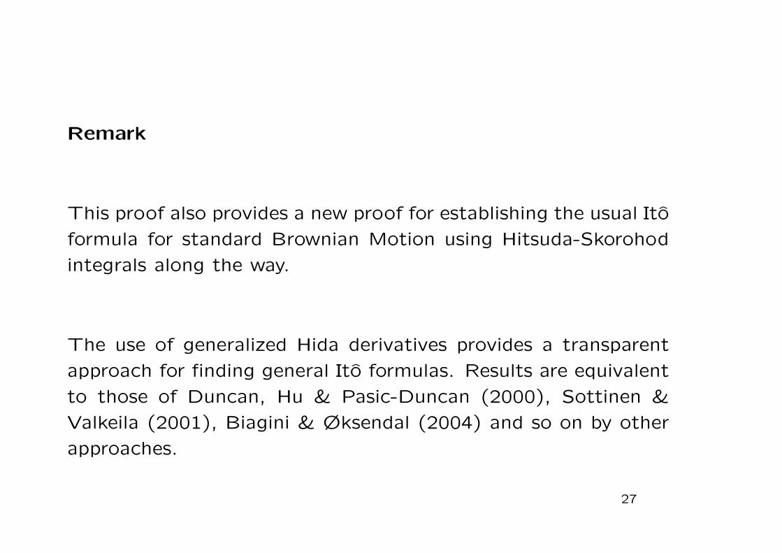
Remark

This proof also provides a new proof for establishing the usual Ito

formula for standard Brownian Motion using Hitsuda-Skorohod

integrals along the way.

The use of generalized Hida derivatives provides a transparent

approach for finding general Ito formulas. Results are equivalent

to those of Duncan, Hu & Pasic-Duncan (2000), Sottinen &

Valkeila (2001), Biagini & Øksendal (2004) and so on by other

approaches.

27

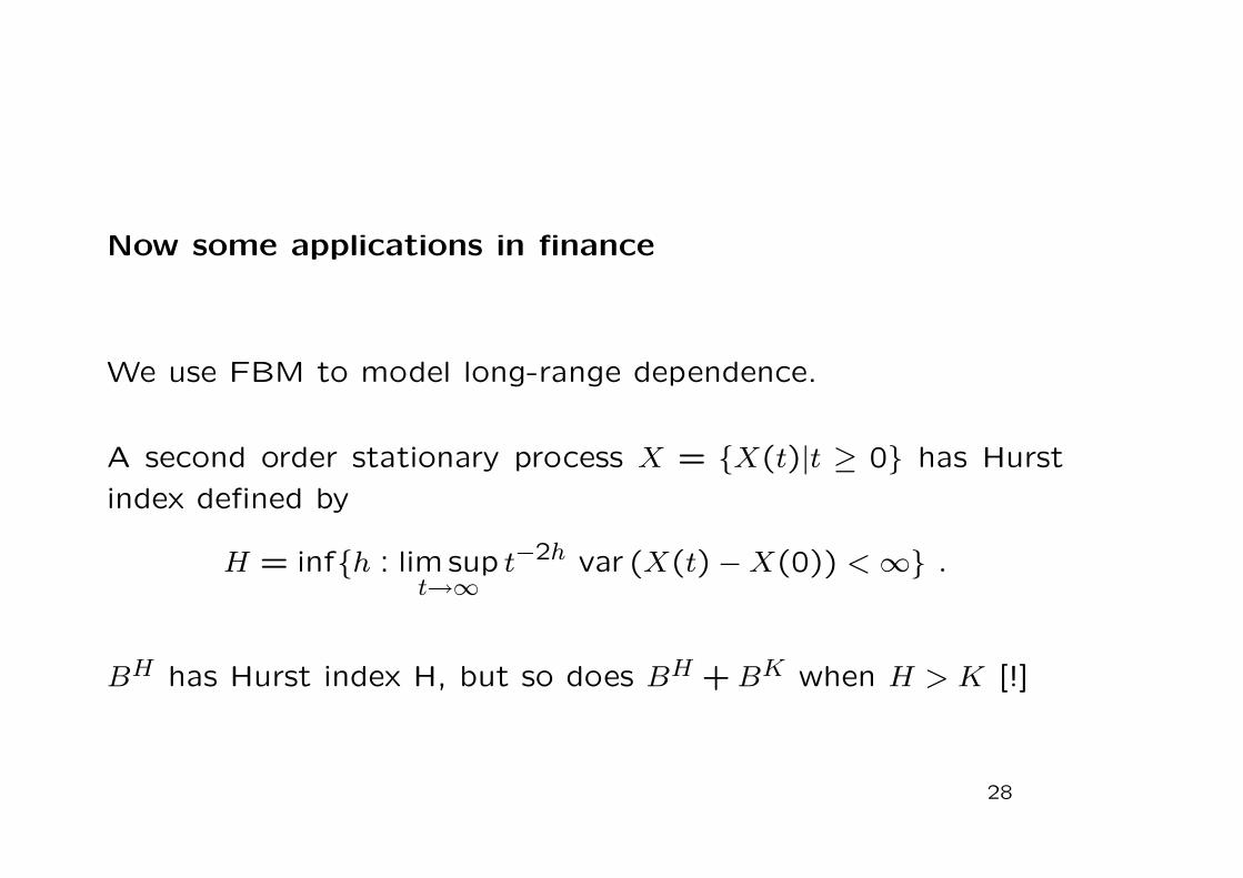
Now some applications in finance

We use FBM to model long-range dependence.

A second order stationary process X = X(t)|t ≥ 0 has Hurst

index defined by

H = infh : lim supt→∞

t−2h var (X(t) −X(0)) <∞ .

BH has Hurst index H, but so does BH +BK when H > K [!]

28

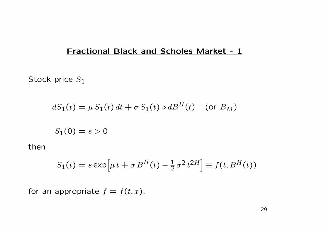
Fractional Black and Scholes Market - 1

Stock price S1

dS1(t) = µS1(t) dt+ σ S1(t) dBH(t) (or BM)

S1(0) = s > 0

then

S1(t) = s exp[µ t+ σ BH(t) − 1

2 σ2 t2H

]≡ f(t, BH(t))

for an appropriate f = f(t, x).

29

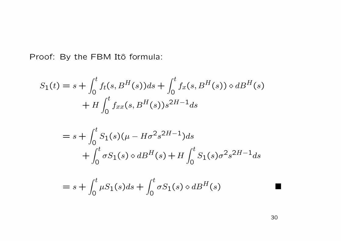
Proof: By the FBM Ito formula:

S1(t) = s+∫ t

0ft(s,B

H(s))ds+∫ t

0fx(s,B

H(s)) dBH(s)

+H∫ t

0fxx(s,B

H(s))s2H−1ds

= s+∫ t

0S1(s)(µ−Hσ2s2H−1)ds

+∫ t

0σS1(s) dBH(s)+H

∫ t

0S1(s)σ

2s2H−1ds

= s+∫ t

0µS1(s)ds+

∫ t

0σS1(s) dBH(s)

30

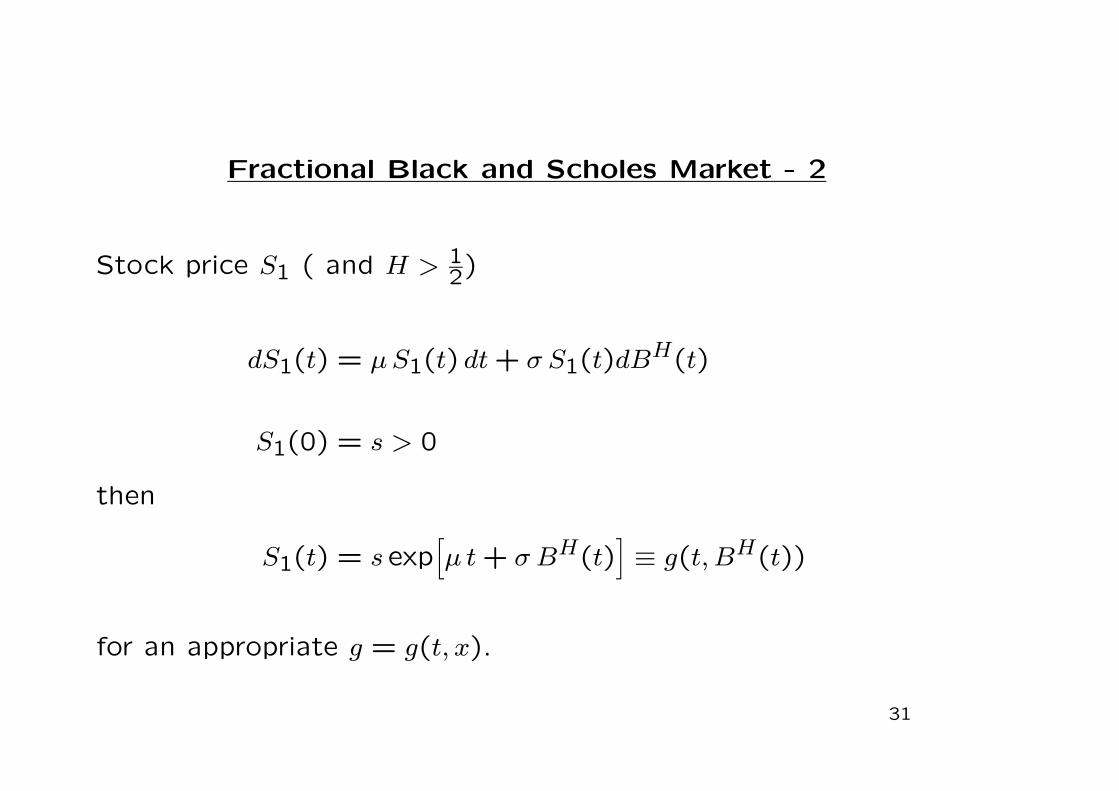
Fractional Black and Scholes Market - 2

Stock price S1 ( and H > 12)

dS1(t) = µS1(t) dt+ σ S1(t)dBH(t)

S1(0) = s > 0

then

S1(t) = s exp[µ t+ σ BH(t)

]≡ g(t, BH(t))

for an appropriate g = g(t, x).

31

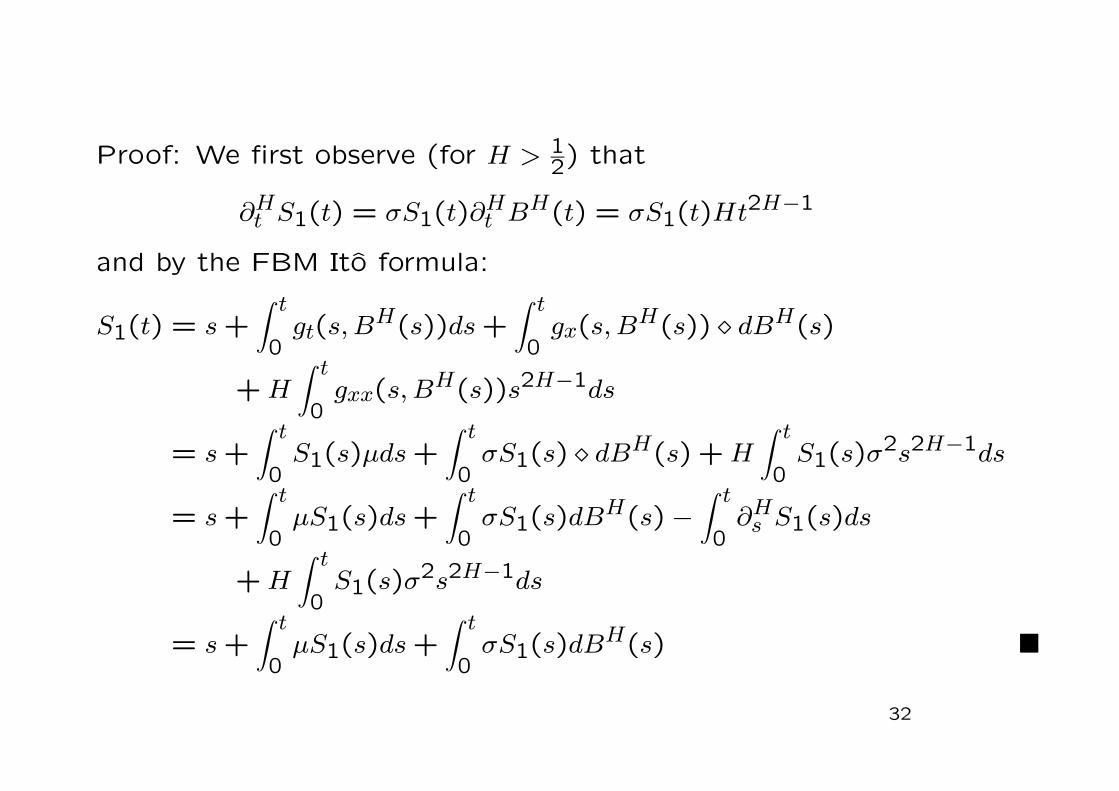
Proof: We first observe (for H > 12) that

∂Ht S1(t) = σS1(t)∂Ht B

H(t) = σS1(t)Ht2H−1

and by the FBM Ito formula:

S1(t) = s+∫ t

0gt(s,B

H(s))ds+∫ t

0gx(s,B

H(s)) dBH(s)

+H∫ t

0gxx(s,B

H(s))s2H−1ds

= s+∫ t

0S1(s)µds+

∫ t

0σS1(s) dBH(s) +H

∫ t

0S1(s)σ

2s2H−1ds

= s+∫ t

0µS1(s)ds+

∫ t

0σS1(s)dB

H(s) −∫ t

0∂Hs S1(s)ds

+H∫ t

0S1(s)σ

2s2H−1ds

= s+∫ t

0µS1(s)ds+

∫ t

0σS1(s)dB

H(s)

32

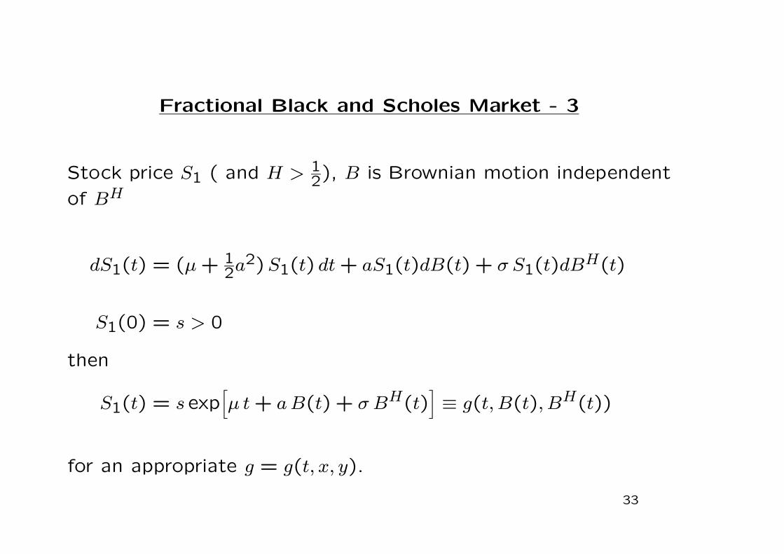
Fractional Black and Scholes Market - 3

Stock price S1 ( and H > 12), B is Brownian motion independent

of BH

dS1(t) = (µ+ 12a

2)S1(t) dt+ aS1(t)dB(t) + σ S1(t)dBH(t)

S1(0) = s > 0

then

S1(t) = s exp[µ t+ aB(t) + σ BH(t)

]≡ g(t, B(t), BH(t))

for an appropriate g = g(t, x, y).

33

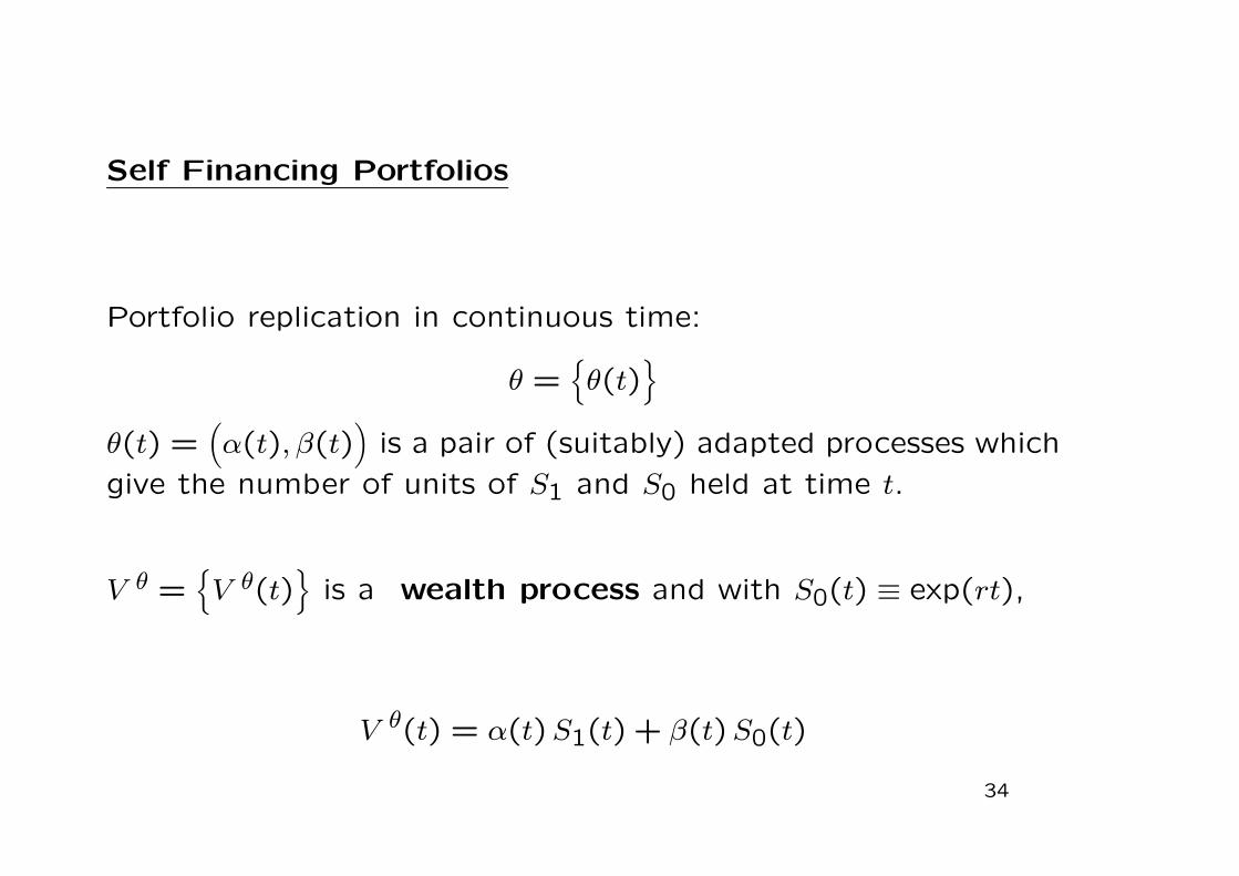
Self Financing Portfolios

Portfolio replication in continuous time:

θ =θ(t)

θ(t) =

(α(t), β(t)

)is a pair of (suitably) adapted processes which

give the number of units of S1 and S0 held at time t.

V θ =V θ(t)

is a wealth process and with S0(t) ≡ exp(rt),

V θ(t) = α(t)S1(t) + β(t)S0(t)

34

θ satisfies certain technical conditions and must be self-financing:

dV θ(t) = α(t) dS1(t) + β(t) dS0(t)

Changes in the wealth process come from changes in the valuesof the underlying assets S0 and S1.

V θ(T ) =[S1(T ) −K

]+

for a European call option, say.

35

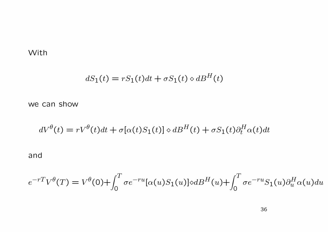
With

dS1(t) = rS1(t)dt+ σS1(t) dBH(t)

we can show

dV θ(t) = rV θ(t)dt+ σ[α(t)S1(t)] dBH(t) + σS1(t)∂Ht α(t)dt

and

e−rTV θ(T ) = V θ(0)+∫ T

0σe−ru[α(u)S1(u)] dBH(u)+

∫ T

0σe−ruS1(u)∂

Hu α(u)du

36

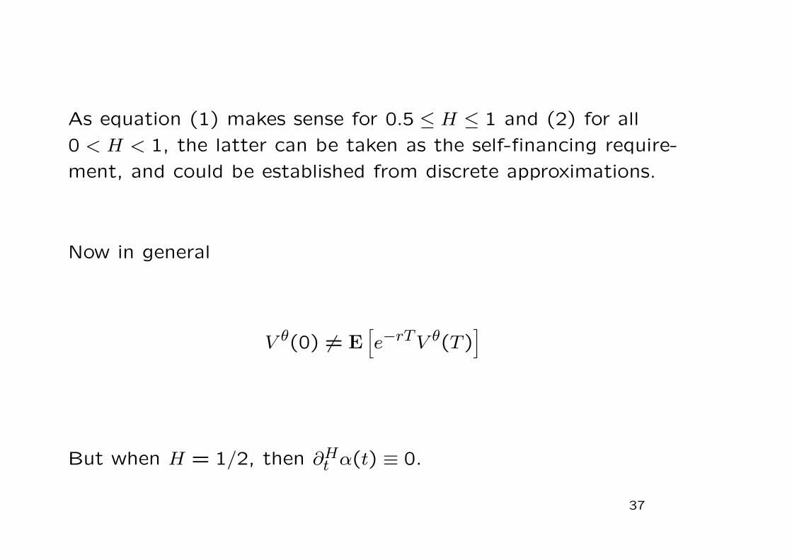
As equation (1) makes sense for 0.5 ≤ H ≤ 1 and (2) for all

0 < H < 1, the latter can be taken as the self-financing require-

ment, and could be established from discrete approximations.

Now in general

V θ(0) = E[e−rTV θ(T )

]

But when H = 1/2, then ∂Ht α(t) ≡ 0.

37

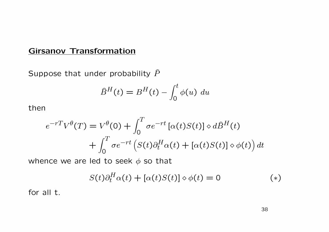
Girsanov Transformation

Suppose that under probability P

BH(t) = BH(t) −∫ t

0φ(u) du

then

e−rTV θ(T ) = V θ(0) +∫ T

0σe−rt [α(t)S(t)] dBH(t)

+∫ T

0σe−rt

(S(t)∂Ht α(t) + [α(t)S(t)] φ(t)

)dt

whence we are led to seek φ so that

S(t)∂Ht α(t) + [α(t)S(t)] φ(t) = 0 (∗)for all t.

38

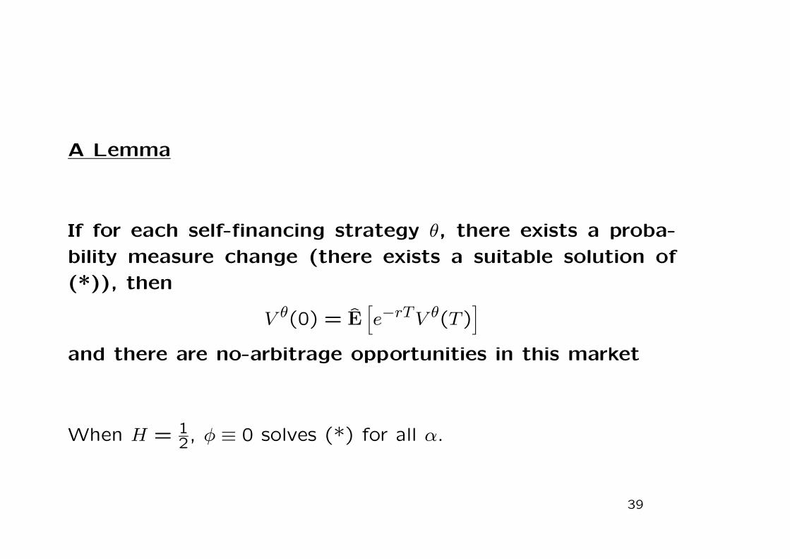
A Lemma

If for each self-financing strategy θ, there exists a proba-

bility measure change (there exists a suitable solution of

(*)), then

V θ(0) = E[e−rTV θ(T )

]and there are no-arbitrage opportunities in this market

When H = 12, φ ≡ 0 solves (*) for all α.

39

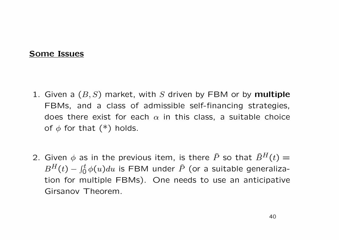
Some Issues

1. Given a (B,S) market, with S driven by FBM or by multiple

FBMs, and a class of admissible self-financing strategies,

does there exist for each α in this class, a suitable choice

of φ for that (*) holds.

2. Given φ as in the previous item, is there P so that BH(t) =

BH(t) − ∫ t0 φ(u)du is FBM under P (or a suitable generaliza-

tion for multiple FBMs). One needs to use an anticipative

Girsanov Theorem.

40

In the (B,S) market, Cheridito(2000) claimed that there are ar-

bitrage opportunities, so one may try to construct α for which

there is no φ. However for some “mixture” models there are no-

arbitrage opportunities (e.g. Kuznetsov(1999), Cheridito(2000),

Androshchuk + Mishura(2005)). For FBM markets, models for

S have to be specified carefully, and the specification of admis-

sible trading strategies.

Our machinery can be adapted to multiple FBM models and

used to study these questions. This is on-going research.

41

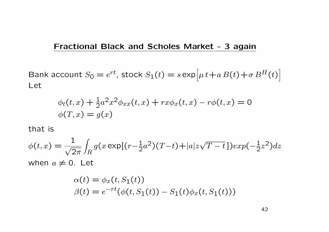
Fractional Black and Scholes Market - 3 again

Bank account S0 = ert, stock S1(t) = s exp[µ t+aB(t)+σ BH(t)

]Let

φt(t, x) + 12a

2x2φxx(t, x) + rxφx(t, x) − rφ(t, x) = 0

φ(T, x) = g(x)

that is

φ(t, x) =1√2π

∫Rg(x exp[(r−1

2a2)(T−t)+|a|z√T − t ])exp(−1

2z2)dz

when a = 0. Let

α(t) = φx(t, S1(t))

β(t) = e−rt(φ(t, S1(t)) − S1(t)φx(t, S1(t)))

42

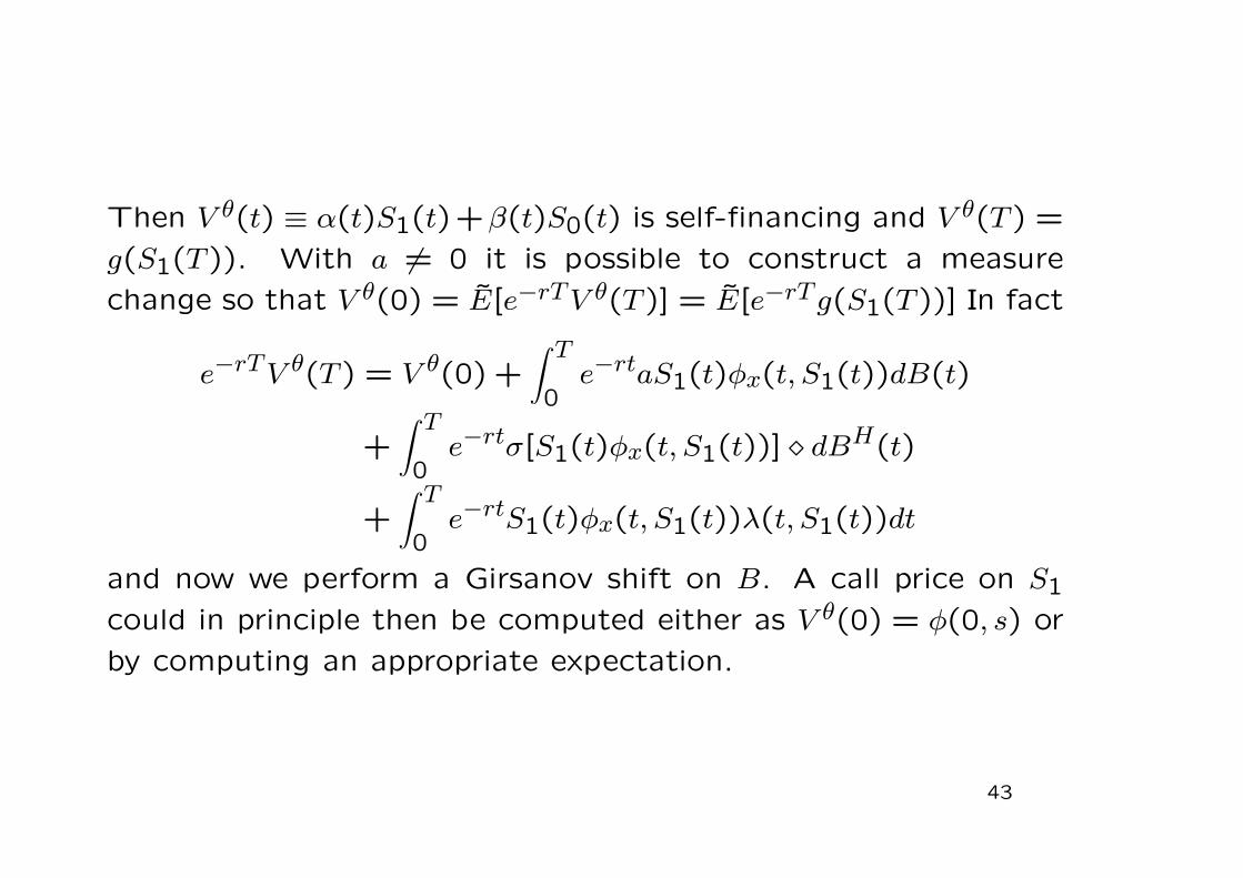
Then V θ(t) ≡ α(t)S1(t)+β(t)S0(t) is self-financing and V θ(T ) =

g(S1(T )). With a = 0 it is possible to construct a measure

change so that V θ(0) = E[e−rTV θ(T )] = E[e−rT g(S1(T ))] In fact

e−rTV θ(T ) = V θ(0) +∫ T

0e−rtaS1(t)φx(t, S1(t))dB(t)

+∫ T

0e−rtσ[S1(t)φx(t, S1(t))] dBH(t)

+∫ T

0e−rtS1(t)φx(t, S1(t))λ(t, S1(t))dt

and now we perform a Girsanov shift on B. A call price on S1

could in principle then be computed either as V θ(0) = φ(0, s) or

by computing an appropriate expectation.

43

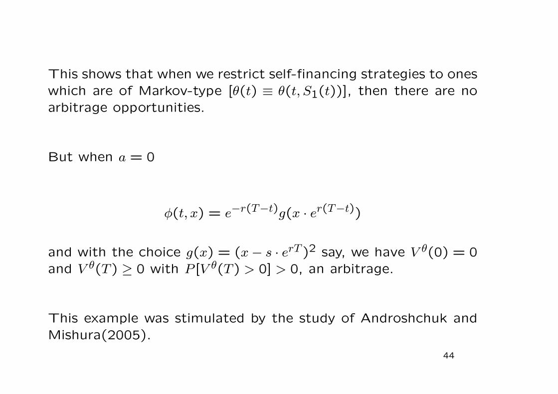
This shows that when we restrict self-financing strategies to oneswhich are of Markov-type [θ(t) ≡ θ(t, S1(t))], then there are noarbitrage opportunities.

But when a = 0

φ(t, x) = e−r(T−t)g(x · er(T−t))

and with the choice g(x) = (x− s · erT )2 say, we have V θ(0) = 0and V θ(T ) ≥ 0 with P [V θ(T ) > 0] > 0, an arbitrage.

This example was stimulated by the study of Androshchuk andMishura(2005).

44

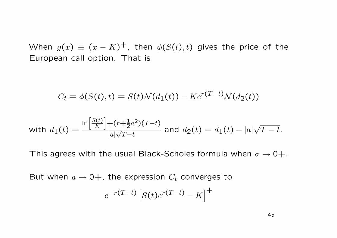
When g(x) ≡ (x − K)+, then φ(S(t), t) gives the price of the

European call option. That is

Ct = φ(S(t), t) = S(t)N (d1(t)) −Ker(T−t)N (d2(t))

with d1(t) =ln

[S(t)K

]+(r+1

2a2)(T−t)

|a|√T−t and d2(t) = d1(t) − |a|√T − t.

This agrees with the usual Black-Scholes formula when σ → 0+.

But when a→ 0+, the expression Ct converges to

e−r(T−t)[S(t)er(T−t) −K

]+45