APPROVED:

Paolo Grigolini, Major Professor Arkadii Krokhin, Committee Member James Roberts, Committee Member Duncan L. Weathers, Committee

Member Floyd McDaniel, Chair of the

Department of Physics Sandra L. Terrell, Dean of the Robert B.

Toulouse School of Graduate Studies

FRACTIONAL BROWNIAN MOTION AND DYNAMIC

APPROACH TO COMPLEXITY

Rasit Cakir

Dissertation Prepared for the Degree of

DOCTOR OF PHILOSOPHY

UNIVERSITY OF NORTH TEXAS

August 2007

Cakir, Rasit, Fractional Brownian motion and dynamic approach to

complexity. Doctor of Philosophy (Physics), August 2007, 103 pp., 42 illustrations,

references, 52 titles.

The dynamic approach to fractional Brownian motion (FBM) establishes a link

between non-Poisson renewal process with abrupt jumps resetting to zero the

system's memory and correlated dynamic processes, whose individual trajectories

keep a non-vanishing memory of their past time evolution. It is well known that the

recrossing times of the origin by an ordinary 1D diffusion trajectory generates a

distribution of time distances between two consecutive origin recrossing times with

an inverse power law with index μ=1.5. However, with theoretical and numerical

arguments, it is proved that this is the special case of a more general condition,

insofar as the recrossing times produced by the dynamic FBM generates process

with μ=2-H. Later, the model of ballistic deposition is studied, which is as a simple

way to establish cooperation among the columns of a growing surface, to show that

cooperation generates memory properties and, at same time, non-Poisson renewal

events. Finally, the connection between trajectory and density memory is discussed,

showing that the trajectory memory does not necessarily yields density memory, and

density memory might be compatible with the existence of abrupt jumps resetting to

zero the system's memory.

Copyright 2007

by

Rasit Cakir

ii

CONTENTS

LIST OF FIGURES v

CHAPTER 1. INTRODUCTION 1

CHAPTER 2. DYNAMIC APPROACH TO FRACTIONAL BROWNIAN MOTION 3

2.1. Di�usion Equation 3

2.2. Long Range Memory over the Stochastic Velocity 4

2.3. Scaling 5

2.4. Renewal Properties 6

2.5. Non-ergodicity 9

CHAPTER 3. NUMERICAL CALCULATIONS 11

3.1. Renewal and Cooperation Model 11

3.2. The Fourier Algorithm 13

3.3. The Voss Algorithm 25

CHAPTER 4. RANDOM SURFACE GROWTH 32

4.1. Collective Properties 34

4.2. Properties of the Jumps 36

4.3. Single Column Properties 38

CHAPTER 5. TRAJECTORY AND DENSITY MEMORY 44

5.1. The Generalized Di�usion Equation from the CTRW Perspective 46

5.2. Auxiliary Fluctuation 50

5.3. On the Dynamical Nature of the Memory Kernel of the Ctrw Generalized

Di�usion Equation 54

5.4. The Stochastic Liouville Approach 57

iii

5.5. Dynamical Origin of the Time Convoluted Di�usion Equation 61

CHAPTER 6. CONCLUSION 65

APPENDIX A. SOLUTION OF THE ORDINARY DIFFUSION EQUATION 67

APPENDIX B. SOLUTION OF THE GENERALIZED DIFFUSION EQUATION

OF FBM 70

APPENDIX C. ASYMPTOTIC SOLUTION OF THE GENERALIZED DIFFUSION

EQUATION OF FBM 73

APPENDIX D. RELATION BETWEEN THE VARIANCE AND THE

STATIONARY CORRELATION FUNCTION OF FBM 75

APPENDIX E. RELATION BETWEEN THE VARIANCE AND THE SCALING

OF FBM 79

APPENDIX F. DIFFUSION ENTROPY 81

APPENDIX G. ON THE PROBABILITY OF THE RECROSSING TIMES 83

APPENDIX H. LAPLACE TRANSFORM OF THE POWER LAW FUNCTION

WITH SLOPE 1 < � < 2 85

APPENDIX I. CORRELATION FUNCTION OF THE DIFFUSION VARIABLE

OF FBM 87

APPENDIX J. RELATION BETWEEN THE MEMORY KERNEL AND THE

POWER LAW DISTRIBUTION OF CTRW 91

APPENDIX K. DERIVATION OF THE AUXILARY FUNCTION 95

APPENDIX L. RELATION BETWEEN THE VARIANCE AND THE MEMORY

KERNEL OF CTRW 98

APPENDIX M. THE FORM OF MEMORY KERNEL OF CTRW 100

REFERENCES 102

iv

LIST OF FIGURES

2.1 Aging experiment. 8

2.2 The correlation of x(t) for normal di�usion, sub- di�usion and super-di�usion. 10

3.1 The correlation function of �(t) for sub-di�usion case, H = 1=3, and

super-di�usion case, H = 2=3, using 107 oscillators in the RC model. 13

3.2 The correlation function of �(t) for the super-di�usion case, H = 2=3. 16

3.3 The correlation function of �(t) for the sub-di�usion case, H = 1=3. 17

3.4 Variance for the super-di�usion case, H = 2=3. 18

3.5 Di�usion entropy for the super-di�usion case, H = 2=3. 18

3.6 Variance for the sub-di�usion case, H = 1=3. 19

3.7 Di�usion entropy for the sub-di�usion case, H = 2=3. 19

3.8 The distributions of recrossing times of x(t). 21

3.9 Correlation functions of recrossing times of x(t) for H = 1=3 and H = 2=3. 21

3.10 Survival probabilities of renewal aging of recrossing times of x(t) for ta = 100. 22

3.11 The distributions of srecrossing time of �(t) for H = 2=3 and for H = 1=3. 23

3.12 Correlation functions of recrossing times of �(t) for H = 1=3 and H = 2=3. 24

3.13 Voss algorithm for m = 3. 25

3.14 The development of x(t) for m = 8. 26

3.15 The correlation functions of the super-di�usion, H = 2=3, and the

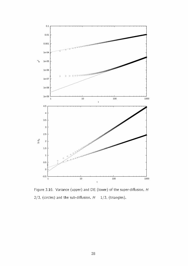
sub-di�usion, H = 1=3, for both normal and log-log scales 27

3.16 Variance and DE of the super-di�usion, H = 2=3, and the sub-di�usion,

H = 1=3. 28

v

3.17 Distributions of recrossing times of x for the super-di�usion, H = 2=3, and

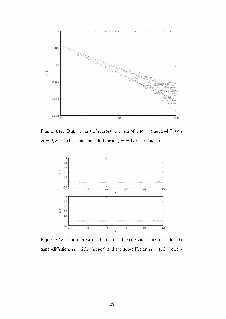
the sub-di�usion, H = 1=3. 29

3.18 The correlation functions of recrossing times of x for the super-di�usion,

H = 2=3, and the sub-di�usion,H = 1=3. 29

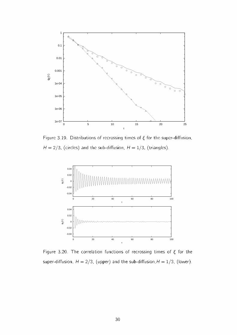
3.19 Distributions of recrossing times of � for the super-di�usion, H = 2=3, and

the sub-di�usion, H = 1=3. 30

3.20 The correlation functions of recrossing times of � for the super-di�usion,

H = 2=3, and the sub-di�usion,H = 1=3. 30

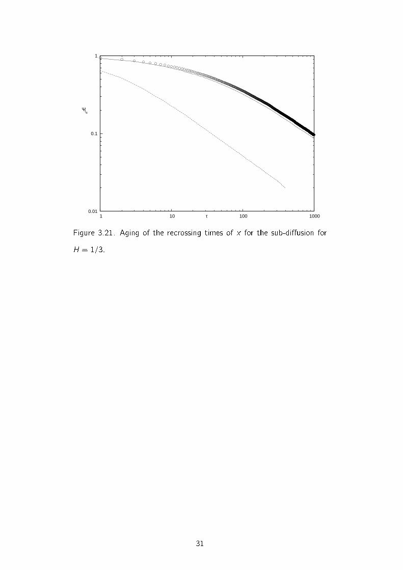
3.21 Aging of the recrossing times of x for the sub-di�usion for H = 1=3. 31

4.1 Model of ballistic deposition. 32

4.2 The surface for L = 1000. 33

4.3 y(t) for L = 1000. 34

4.4 Standard deviation of y(t). 35

4.5 Correlation function of recrossing times of y(t) for L = 1000. 35

4.6 Probability distribution of recrossing times of y(t) when there is aging and

no aging. 36

4.7 Probability distribution of jumps and recrossing of jumps of a single column

in ballistic deposition. 37

4.8 Correlation function of jumps in ballistic deposition for L = 1000 and for

� > 0 and � > 1. 38

4.9 x(t) for L = 1000. 39

4.10 Standard deviation of x for L = 1000. 39

4.11 Standard deviation of x and y for L = 200. 40

4.12 Correlation function of recrossing times of x(t) for L = 1000. 40

4.13 Probability distribution of recrossing times of x(t) when there is aging and

no aging. 41

vi

4.14 Correlation function of ~�(t) for L = 1000. 42

5.1 Auxiliary uctuation �A(t) for � = 1:666 and � = 0:01. 52

5.2 Plot of the motion in Eq. 5.32 for � = 1:666 and � = 0:01. 52

5.3 The time evolution of the second moment of x(t) for CTRW. 53

5.4 F (t)=t2�� and 1=t3��. 57

5.5 Time asymptotic properties of the correlation function of dichotomous

uctuation and original uctuation for H = 1=3. 62

5.6 The DF property of Eq.5.66. 63

vii

CHAPTER 1

INTRODUCTION

This thesis addresses the problem of the dynamic approach to fractional Brownian

motion (FBM), for the main purpose of shedding light into some misleading opinions that

have been haunting this subject, since the original work of Mandelbrot and Van Ness [1].

In fact, FBM is generally considered to be a process generating anomalous di�usion,

either faster or slower than ordinary di�usion, as a consequence of in�nite memory. This

in�nite memory is usually considered to be incompatible with the renewal properties that

many physical processes, from blinking quantum dots (BQD) to the random growth of

surfaces [2], are revealing with increasing theoretical and experimental evidence.

The �rst part of this thesis proves that memory resides in the velocity variable, whose

uctuations generate the di�usion process, whose time asymptotic properties, in turn,

become indistinguishable from the FBM prescription. The space variable x , in the scaling

limit, becomes a renewal variable. Studying the crossings of the space origin, x = 0, and

recording the times at which the crossings occur, it can be proved that the space variable,

x , is a time sequence that is a non-ergodic, non-Poisson process. The rigorous proof of

this important property is obtained by applying to the recorded sequence a method of

analysis, called aging experiment, which has been applied with success to the BQD data

to prove rigorously their renewal nature. As a consequence of our analysis, the process

of x-axis recrossing is proved to be renewal and non-ergodic. In conclusion, the �rst

result proved by this thesis is that the supposedly in�nite memory of FBM is the physical

manifestation of ergodicity breakdown.

The second part of this thesis is a review of some work recently done in the �eld of

random growth of interfaces and proves that the process of random growth of interfaces

shares the same properties as dynamic FBM, with the coexistence of memory and renewal

properties.

1

Finally, the third part of the thesis addresses theoretical issues concerning the formal

equivalence between the generalized master equation of renewal origin and the generalized

master equation of memory origin. It proves that, in spite of the formal equivalence, these

processes are di�erent and the conjecture is made that they will yield di�erent responses

to external perturbations.

2

CHAPTER 2

DYNAMIC APPROACH TO FRACTIONAL BROWNIAN MOTION

FBM is a random process with long memory dependence and with a de�ned scaling.

In this chapter, a dynamic approach to FBM is proposed, to prove that despite a general

conviction to the contrary this generates renewal events.

2.1. Di�usion Equation

The representation of the Brownian motion by means of probability yields,

(2.1)@@tpB(x; t) = D

@2

@x2pB(x; t);

which is the normal di�usion process, where p(x; t) is the probability density and D is

the di�usion constant (App. A). The solution is well known.

(2.2) pB(x; t) =1p

4�Dtexp

(� x2

4Dt

):

FBM can be obtained by generalizing BM as

(2.3) p(x; t) =1p

4�Dt2Hexp

(� x2

4Dt2H

);

where 0 < H < 1. When H = 1=2, it becomes a normal di�usion process.

Let us consider a general form of the di�usion equation:

(2.4)@@t

~p(x; t) = D(∫ t

0d���(�)

)@2

@x2 ~p(x; t) = D(t)@2

@x2 ~p(x; t);

where �� is the correlation function of the stochastic noise which will be de�ned later.

The solution of this equation is (App. B)

(2.5) ~p(x; t) =1√

2�D < x2(t) >exp

(� x2(t)

2D < x2(t) >

):

In App. C, it is also shown that, when t !1, p(x; t) is the solution of the general

di�usion equation. Since limt!1 p(x; t) = ~p(x; y), FBM has long time scale property.

3

2.2. Long Range Memory over the Stochastic Velocity

Let us consider the equation of free di�usion.

(2.6)ddtx(t) = �(t)

The Gaussian random variable � can be thought of the stochastic velocity of a particle

with a time independent Gaussian distribution of zero average and constant variance.

(2.7) p(�) =1√

2� h�2i exp(� �2

2 h�2i):

The properties of the position of the particle, x , simply depend on �. The trajectory for a

single particle is a uctuation around zero so that < x >= 0. Calculation of the variance

�2 =< x2 > by using x(t) =∫ t

0 �(t 0)dt 0 + x(0) gives

(2.8) < x2 >=∫ t

0dt 0

∫ t

0dt 00 < �(t 0)�(t 00) >;

where � and x(0) are uncorrelated. Using the de�nition of the correlation function,

(2.9) ��(t 0; t 00) � < �(t 0)�(t 00) >< �2 >

:

Eq. 2.8 turns into (App. D)

(2.10) < x2 >= 2 < �2 >∫ t

0dt 0

∫ t 0

0dt 00��(t 00):

In case of ordinary BM, �(t) is uncorrelated random variable so ��(t) = �(t), which

gives

(2.11) < x2 >= 2 < �2 > t:

Since there is no dissipating force, x is growing withpt because of the uctuation.

In FBM, ��(t) is no longer a delta function. Since FBM has long range memory,

the auto-correlation of � is chosen as power law. If we calculate the variance, < x2 >=∫1�1 x2p(x; t)dx , using Eq. 2.3, we obtain (App. E)

(2.12) < x2(t) >= 2Dt2H:

For H = 1=2, < x2(t) >= 2Dt, which gives D =< �2 >.

4

Let us go back to Eq. 2.10 for FBM. The second derivative of it is

(2.13)d2

dt2 < x2 >= 2 < �2 > ��(t):

The function �(t) is a stochastic process with power law correlation, ��(t) / 1=t�. Let

us take the derivative of Eq 2.12.

(2.14)d2

dt2 < x2 >= 2D2H(2H � 1)t2H�2 = 2 < �2 > ��(t) / 1=t�:

The relation between the scaling and the power law correlation of � is obtained as

(2.15) � = 2� 2H

and the coe�cient becomes negative when H < 1=2. The general form of the correlation

function becomes

(2.16) ��(t) /

1=t� for 1 > H > 1=2, super-di�usion;

�(t) for H = 1=2, normal di�usion;

�1=t� for 0 < H < 1=2, sub-di�usion:

When H > 1=2, x di�uses faster than the normal di�usion, which is called super-di�usion.

Because of the positive correlation of �, particles tend to di�use in the same direction.

And when H < 1=2, x di�uses slower than the normal di�usion, which is called sub-

di�usion. For H 6= 1=2, �(t) has long range memory that is the reason of the anomalous

di�usion.

2.3. Scaling

The scaling from the probability distribution function is de�ned as � by

(2.17) p(x; t) =1t�F

( xt�

);

where F is an arbitrary function. So Eq. 2.3 gives the scaling � = H. Di�usion entropy

(DE) calculations determine the scaling through the property (App. F):

(2.18) S(t) = �∫p ln(p)dx = A+ � ln(t):

5

The scaling can also be determined using the variance. The variance is de�ned as

(2.19) < x2 >=∫ 1

�1x2p(x; t)dx:

From App. E, we get

(2.20) < x2 >= 2Dt2H:

Since the scaling is an asymptotic property, variance and DE will reach the scaling

regime when t !1. In this work, scaling will be represented as H.

2.4. Renewal Properties

2.4.1. Recrossing Times

The renewal properties of FBM will be �rst shown by the recrossing times of x(t) and

�(t). Recrossing times of a function f is the time distance � between successive time

value when f (t) = 0. Let us �rst make the critical assumption, which will be checked

numerically, that in the scaling regime of Eq. 2.17 the process is renewal, which means

that recrossing times of x(t) are statistically independent.

The trajectory x(t), which at t = 0 starts from x = 0, contributes to the probability

p(0; t), due to successive recrossing of the x axes at later times. The rate of occurrence

of recrossing times is the density at the origin and it can be written as follows (Eq. 2.3):

(2.21) R(t) = p(0; t) / 1=tH:

The distribution of recrossing times will be assumed to be given by the power law

(2.22) (�) = (�� 1)T ��1

(T + �)�;

where T is a constant that de�nes the time scale. Let us �nd the relation between

� and H. The rate of occurrence of recrossing times is the summation of all possible

recrossing times that occur n times with the last occurring exactly at time t.

(2.23) R(t) =1∑n=1

n(t):

6

With this equation, it is assumed that at this time at least one collision occurs after the

initial time. Using (App. G)

(2.24) n(u) = ( (u))n;

Eq. 2.23 can be rewritten as

(2.25) R(t) =1∑n=1

n(u) =1∑n=1

( (u)

)n:

Because of the normalization,∫1

0 (t)dt = 1, with u > 0, (u) =∫1

0 exp(�ut) (t)dt

is a number smaller than 1. Therefore, Eq. 2.25 yields

(2.26) R(t) = (u)

1� (u):

Using power law assumption and from Eq. H.5 in App. H, we have

(2.27) limu!0

(u)1� (u)

� 1� �(2� �)T ��1u��1

1� (1� �(2� �)T ��1u��1)� 1

�(2� �)T ��1u��1 / u1��:

Comparing Eq. 2.21 and Eq. 2.27, and using L[t�H] = �(1�H)uH�1, we get

(2.28) uH�1 / u1��:

so for long time scale

(2.29) H = 2� �:

This relation has been originally derived using FBM theory, and therefore it was

considered to imply trajectory memory on x . We will see that this is not so.

2.4.2. Renewal Aging

The renewal properties of FBM can also be shown by the aging calculation. To see

what is aging, let us look at Fig. 2.1. The time distances �i are from the distribution of

recrossing times, (�).

Consider an ensemble number of the trajectory x(t). Each of the time values of

x(t) = 0 is considered as an event. If the observation starts at t = 0, which is also an

event, the time until next event is �1. So this time is selected from the distribution, (�).

But, if the observation starts from an arbitrary time ta > 0, which is not necessarily an

7

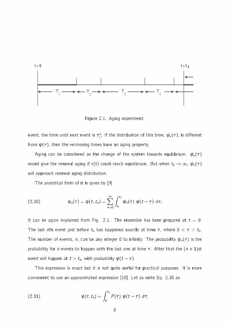
Figure 2.1. Aging experiment.

event, the time until next event is �a1 . If the distribution of this time, a(�), is di�erent

from (�), then the recrossing times have an aging property.

Aging can be considered as the change of the system towards equilibrium. a(�)

would give the renewal aging if x(t) could reach equilibrium. But when ta ! 1, a(�)

will approach renewal aging distribution.

The analytical form of it is given by [9]

(2.30) a(�) = (t; ta) =1∑n=0

∫ ta

0 n(�) (t � �) d�:

It can be again explained from Fig. 2.1. The ensemble has been prepared at t = 0.

The last nth event just before ta has happened exactly at time � , where 0 < � < ta.

The number of events, n, can be any integer 0 to in�nity. The probability n(�) is the

probability for n events to happen with the last one at time � . After that the (n + 1)st

event will happen at t > ta, with probability (t � �).

This expression is exact but it is not quite useful for practical purposes. It is more

convenient to use an approximated expression [10]. Let us write Eq. 2.30 as

(2.31) (t; ta) =∫ ta

0P (�) (t � �) d�;

8

where

(2.32) P (�) =1∑n=0

n(�):

The meaning of P (�) is the probability of an event to occur at t. The Laplace transform

of P (�) has been done for 1 < � < 2. Using App. G, Eq. 2.26 and Eq. 2.27,

(2.33) P (u) =1∑n=0

n(u) =1∑n=0

( (u))n =1

1� (u)� 1

�(2� �)T ��1u��1 :

The inverse Laplace transform simply is

(2.34) P (t) � 1�(2� �)T ��1

1�(�� 1)

1t2��

and �nally Eq. 2.30 becomes

(2.35) (t; ta) � 1�(2� �)T ��1�(�� 1)

∫ ta

0

1t2�� (t � �) d�:

In the numeric calculations, P (t) is considered as constant; therefore

(2.36) (t; ta) � N∫ ta

0 (t � �) d�

is used to compare the simulation results.

2.5. Non-ergodicity

The correlation of x(t) can be obtained from the variance. (App. I)

(2.37) �(t; t0) =< x(t)x(t0) >< x2(t0) >

=12

((tt0

)2H

+ 1�(tt0� 1

)2H)

Let us put t ! t and t0 ! �t. Eq. 2.37 becomes

(2.38)< x(t)x(�t) >< x2(t) >

= 1� 22H�1

When, H = 1=2, for BM, Eq. 2.38 becomes zero and it is non-zero otherwise. This has

been considered a non-Markovian process with the well known property of non-decaying

correlations between future and past [5][6]. And, this property has been accepted as the

memory of individual trajectories because it is zero for BM and nonzero for H 6= 1=2.

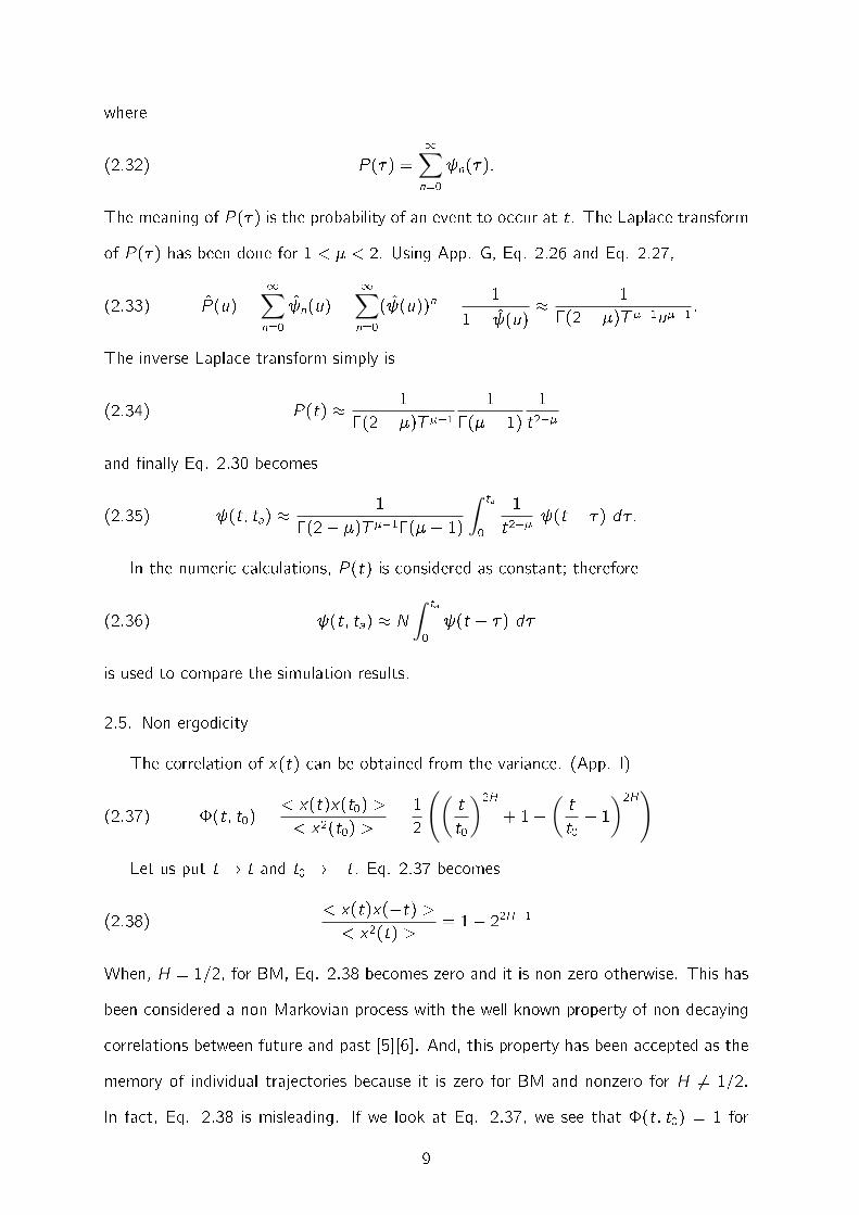
In fact, Eq. 2.38 is misleading. If we look at Eq. 2.37, we see that �(t; t0) = 1 for

9

H = 1=2, which means that the equation being constant doesn't mean memory. Fig.

2.2 shows that there is positive correlation for all of the three cases.

The reason is that the average over ensembles does not a�ord information about the

trajectory x(t), because x(t) is not ergodic. Since the correlation function in Eq. 2.37

depends on the initial time t0, we have

(2.39) �(t; t0) 6= �(jt � t0j);

which means x(t) is not stationary. For a single trajectory x(t) tends to be usually

positive or negative but we know that < x >= 0 so we cannot use the equivalence of

time and ensemble averages. The average over the trajectory time keeps changing and

does not give the ensemble average. Eq. 2.38 does not depend on the trajectory memory.

It depends on the non-ergodic nature of the process. The numerical calculations, indeed,

show that x(t) is renewal, implying that the trajectory does not have memory.

0.6

0.8

1

1.2

1.4

1.6

1.8

2

0 2 4 6 8 10

Φ

t

H=0.5

H=2/3

H=1/3

Figure 2.2. The correlation of x(t) for normal di�usion, sub- di�usion and

super-di�usion. t0 = 1.

10

CHAPTER 3

NUMERICAL CALCULATIONS

3.1. Renewal and Cooperation Model

The Renewal and Cooperation (RC) model is is based on the equation

(3.1) _x = �(t):

The stochastic variable �(t) has a long-range correlation, < �(t)�(t 0) >= �20��(t � t 0).

The long-range properties of the variable �(t) are determined by cooperation. The

variable x is responsible for renewal.

Let us illustrate �rst the cooperative and memory properties of the RC model. �(t)

is derived from the non-Ohmic bath [3]

(3.2) �(t) =∑

i

ci[xi(0) cos!it + vi(0)!�1

i sin!it]:

Here xi(0) and vi(0) are randomly selected from the canonical distribution exp[�(!2i x2i +

v 2i )=kBT )]=Z, and c2

i = !��1i .

Let us assume that the frequencies !i range from !0 = 0 to !D and let us divide the

interval [0; !D] into N small intervals as

(3.3) !i =iN!D:

The average on the Gibbs ensemble, since di�erent oscillators are uncorrelated, yields

(3.4) h�(t)�(t 0)i =∑

i

c2i

[⟨x2i (0)

⟩cos(!it) cos(!it 0) +

hv 2i (0)i!2i

sin(!it) sin(!it 0)]:

The adoption of the canonical condition yields

(3.5)⟨v 2i

⟩= !2

i

⟨x2i

⟩= kbT:

11

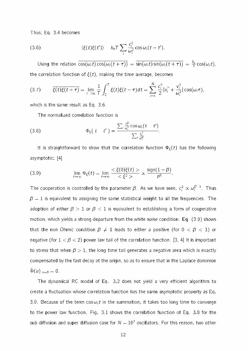
Thus, Eq. 3.4 becomes

(3.6) h�(t)�(t 0)i = kbT∑

i

c2i

!2i

cos!i(t � t 0):

Using the relation cos(!it) cos(!i(t + �)) = sin(!it) sin(!i(t + �)) = �i j2 cos(!it),

the correlation function of �(t), making the time average, becomes

(3.7) �(t)�(t + �) = limT!1

1T

∫ T

0�(t)�(t + �)dt =

N∑

i=1

c2i

2[x2i +

v 2i

!2i

] cos(!i�);

which is the same result as Eq. 3.6.

The normalized correlation function is

(3.8) ��(jt � t 0j) =

∑ic2i!2i

cos!i(t � t 0)∑

ic2i!2i

:

It is straightforward to show that the correlation function ��(t) has the following

asymptotic: [4]

(3.9) limt!1��(t) = lim

t!1< �(0)�(t) >< �2 >

/ sign(1� �)t�

:

The cooperation is controlled by the parameter �. As we have seen, c2i / !��1

i . Thus

� = 1 is equivalent to assigning the same statistical weight to all the frequencies. The

adoption of either � > 1 or � < 1 is equivalent to establishing a form of cooperative

motion, which yields a strong departure from the white noise condition. Eq. (3.9) shows

that the non-Ohmic condition � 6= 1 leads to either a positive (for 0 < � < 1) or

negative (for 1 < � < 2) power law tail of the correlation function. [3, 4] It is important

to stress that when � > 1, the long-time tail generates a negative area which is exactly

compensated by the fast decay at the origin, so as to ensure that in the Laplace dominion

�(u)ju=0 = 0.

The dynamical RC model of Eq. 3.2 does not yield a very e�cient algorithm to

create a uctuation whose correlation function has the same asymptotic property as Eq.

3.9. Because of the term cos!it in the summation, it takes too long time to converge

to the power law function. Fig. 3.1 shows the correlation function of Eq. 3.8 for the

sub-di�usion and super-di�usion case for N = 107 oscillators. For this reason, two other

12

-0.4

-0.2

0

0.2

0.4

0.6

0.8

1

0 20 40 60 80 100

Φ

t

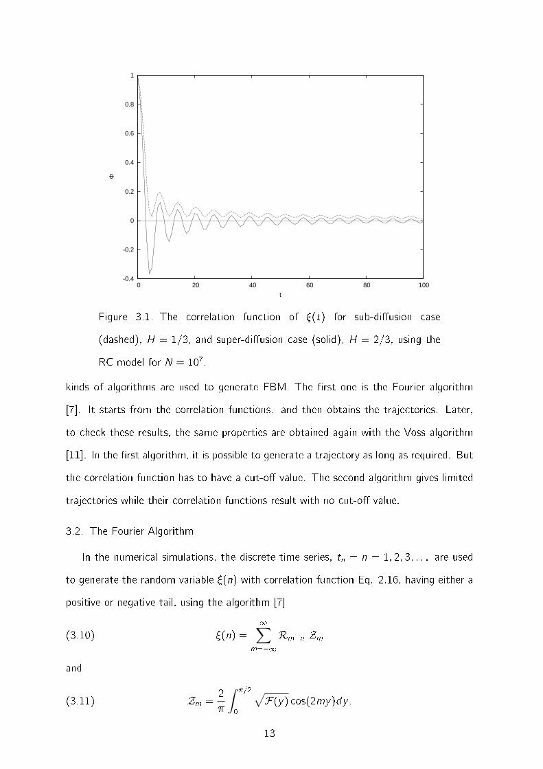
Figure 3.1. The correlation function of �(t) for sub-di�usion case

(dashed), H = 1=3, and super-di�usion case (solid), H = 2=3, using the

RC model for N = 107.

kinds of algorithms are used to generate FBM. The �rst one is the Fourier algorithm

[7]. It starts from the correlation functions. and then obtains the trajectories. Later,

to check these results, the same properties are obtained again with the Voss algorithm

[11]. In the �rst algorithm, it is possible to generate a trajectory as long as required. But

the correlation function has to have a cut-o� value. The second algorithm gives limited

trajectories while their correlation functions result with no cut-o� value.

3.2. The Fourier Algorithm

In the numerical simulations, the discrete time series, tn = n = 1; 2; 3; : : : are used

to generate the random variable �(n) with correlation function Eq. 2.16, having either a

positive or negative tail, using the algorithm [7]

(3.10) �(n) =1∑

m=�1Rm+n Zm

and

(3.11) Zm =2�

∫ �=2

0

√F(y) cos(2my)dy:

13

Here, Rn are Gaussian random numbers with < Rn >= 0 and < R2n >= 1, and Zm =

Z�m. The function F(y) is determined through its Fourier series,

(3.12) F(y) = 1 + 21∑

k=1

��(k) cos(2ky):

Starting from the correlation function �� and using the above algorithm, the series �(n)

and the di�usion trajectory

(3.13) x(n) =n∑

k=1

�(k)

are easily generated.

For the super-di�usion case, �� is chosen as

(3.14) ��(t) =(

TT + t

)�

where� = 2� 2H = 2=3

H = 2=3

T = 1

The correlation function starts from one and is positive since super-di�usion requires

positive correlation.

For the sub-di�usion case, �� is chosen as

(3.15) ��(t) =1b

(T�e��t

� � 1�

(T

T + t

)�)

where� = 2� 2H = 4=3

H = 1=3

T = 1

b = (T� + 1� �)=(� � 1) = 2

� = 1 > (� � 1)=T

The correlation function starts from one and it has a negative tail since sub-di�usion

requires negative correlation. Note that the parameter values are close so as to ensure∫1

0 ��(t)dt = 0 for sub-di�usion. In fact, the negative value is unphysical and it would

produce ordinary di�usion in the long time limit.

14

The index k in Eq. 3.12 goes to 1000 and also m in Eq. 3.10 is in the range

�1000 < m < 1000 so the correlation functions are cut at t = 1000. At the end, the

stochastic x and � values are obtained for required time values.

These analytical forms of �� in Eq. 3.14 and 3.15, and the results from the algorithm

are compared in Fig. 3.2 and Fig. 3.3. They are plotted in normal and log-log scales to

see the values in short and long times.

Variance and DE calculations in Figs. 3.4, 3.6, 3.5 and 3.7 yield the correct slopes,

approaching the expected scaling values, until the cut-o� time. After that they show

that normal di�usion is obtained.

15

0

0.1

0.2

0.3

0.4

0.5

0.6

0.7

0.8

0.9

1

0 20 40 60 80 100

Φ ξ

t

0.001

0.01

0.1

1

1 10 100 1000

Φ ξ

t

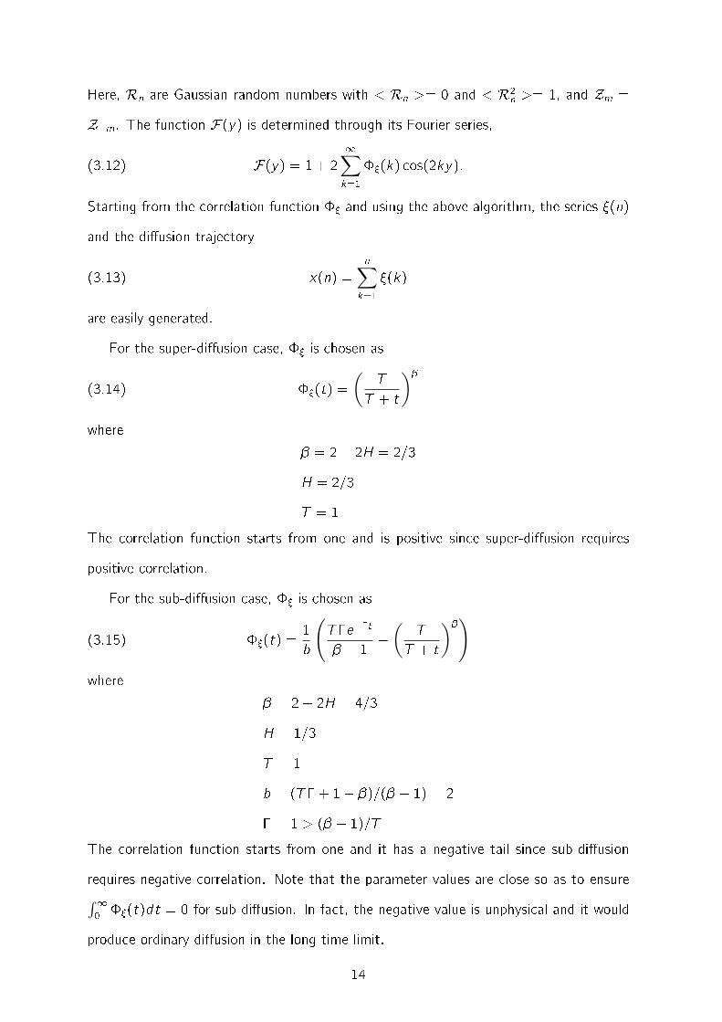
Figure 3.2. The correlation function of �(t) for the super-di�usion case,

H = 2=3 in normal (top) and log-log (bottom) scale. The analytical forms

are solid lines and the correlations from the algorithm are circles and dashed

line.

16

-0.2

0

0.2

0.4

0.6

0.8

1

0 20 40 60 80 100

Φ ξ

t

1e-06

1e-05

1e-04

0.001

0.01

0.1

10 100 1000

Φ ξ

t

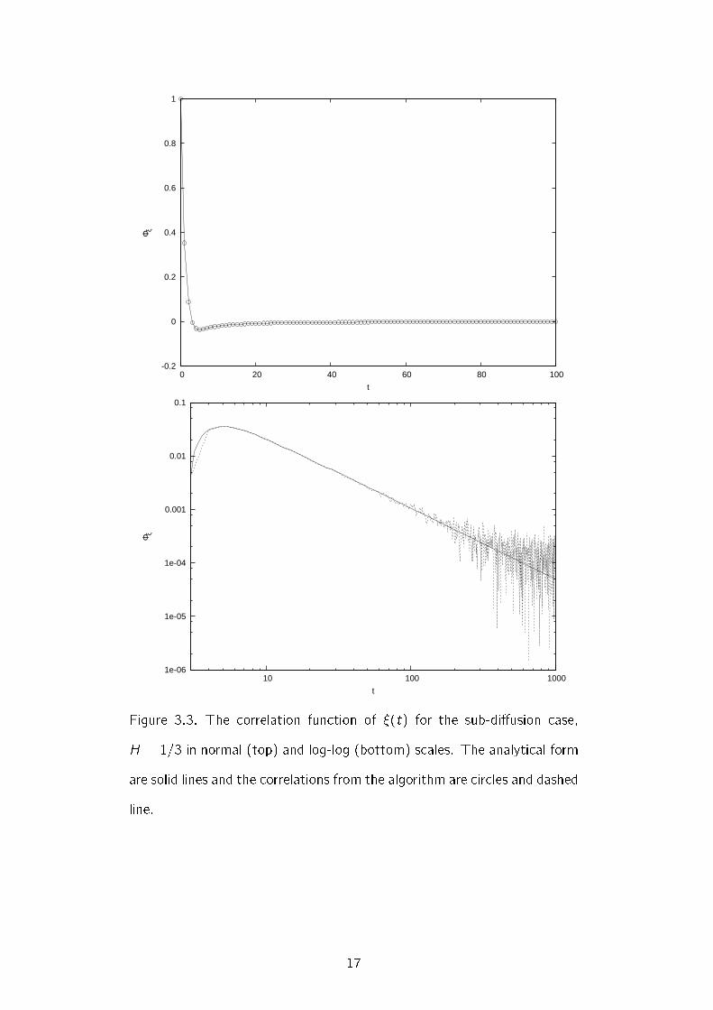
Figure 3.3. The correlation function of �(t) for the sub-di�usion case,

H = 1=3 in normal (top) and log-log (bottom) scales. The analytical form

are solid lines and the correlations from the algorithm are circles and dashed

line.

17

0.1

1

10

100

1000

10000

100000

1e+06

1 10 100 1000 10000

σ2

t

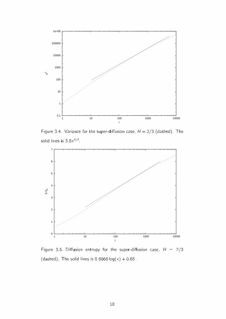
Figure 3.4. Variance for the super-di�usion case, H = 2=3 (dashed). The

solid lines is 3:8x4=3.

0

1

2

3

4

5

6

7

1 10 100 1000 10000

S-S

0

t

Figure 3.5. Di�usion entropy for the super-di�usion case, H = 2=3

(dashed). The solid lines is 0:6666 log(x) + 0:65 .

18

0.1

1

10

100

1000

10000

1 10 100 1000 10000

σ2

t

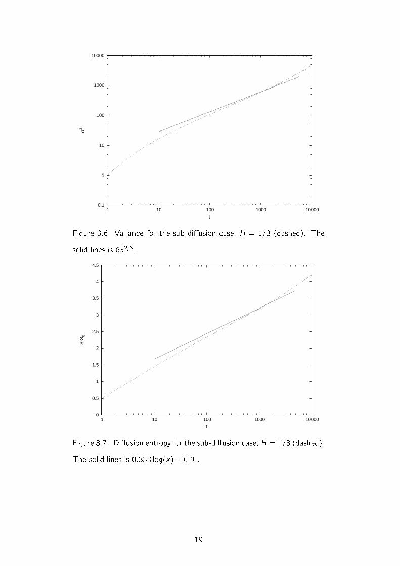
Figure 3.6. Variance for the sub-di�usion case, H = 1=3 (dashed). The

solid lines is 6x2=3.

0

0.5

1

1.5

2

2.5

3

3.5

4

4.5

1 10 100 1000 10000

S-S

0

t

Figure 3.7. Di�usion entropy for the sub-di�usion case, H = 1=3 (dashed).

The solid lines is 0:333 log(x) + 0:9 .

19

The numerical results in Fig. 3.8 show that distribution of recrossing times of x(t)

reaches a power law for larger time values and recrossing times are delta correlated as

shown in Fig. 3.9.

The aging properties are calculated using Eq. 2.36 and are also obtained by aging

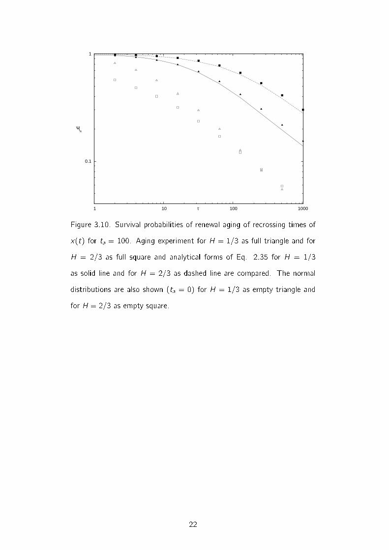
experiment as in Fig. 2.1. Fig. 3.10 shows the survival probabilities, a(�), of recrossing

times of H = 1=3 and H = 2=3 for ta = 100 and ta = 0, where

(3.16) a(�) = (�; ta) = 1�∫ �

0 (�; ta) =

∫ 1

� (�; ta)

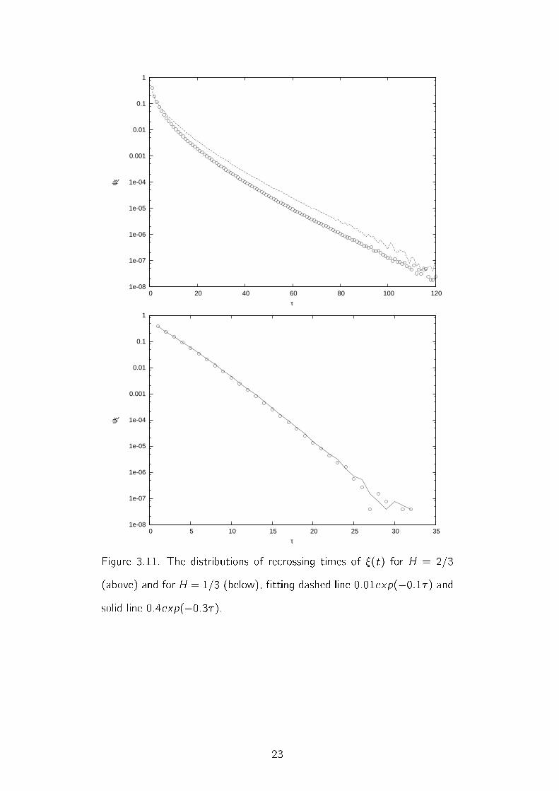
For the case of �(t), the distribution of recrossing times is exponential, which is shown

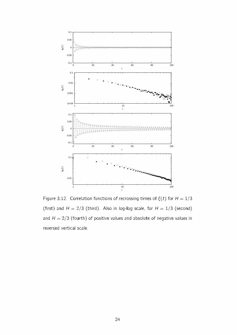
in Fig. 3.11. There is also correlation of recrossing times in Fig. 3.12 due to the memory

on the trajectory �(t). They are also plotted in log scale to see the oscillatory decrease

in power law.

20

10-5

10-4

10-3

10-2

10 100 1000τ

ψ

Figure 3.8. The distributions of recrossing times of x(t) for H = 1=3

(triangle) and for H = 2=3 (square). The former and the latter conditions

�t solid line 2��5=3 and dashed line 0:7��4=3

0

1

0 5 10

0

1

0 5 10

Figure 3.9. Correlation functions of recrossing times of x(t) for H = 1=3

(top) and H = 2=3 (bottom).

21

0.1

1

1 10 100 1000τ

Ψta

Figure 3.10. Survival probabilities of renewal aging of recrossing times of

x(t) for ta = 100. Aging experiment for H = 1=3 as full triangle and for

H = 2=3 as full square and analytical forms of Eq. 2.35 for H = 1=3

as solid line and for H = 2=3 as dashed line are compared. The normal

distributions are also shown (ta = 0) for H = 1=3 as empty triangle and

for H = 2=3 as empty square.

22

1e-08

1e-07

1e-06

1e-05

1e-04

0.001

0.01

0.1

1

0 20 40 60 80 100 120

ψ ξ

τ

1e-08

1e-07

1e-06

1e-05

1e-04

0.001

0.01

0.1

1

0 5 10 15 20 25 30 35

ψ ξ

τ

Figure 3.11. The distributions of recrossing times of �(t) for H = 2=3

(above) and for H = 1=3 (below), �tting dashed line 0:01exp(�0:1�) and

solid line 0:4exp(�0:3�).

23

-0.1

-0.05

0

0.05

0.1

0 20 40 60 80 100φ ξ

(τ)

τ

1e-04

0.001

0.01

0.1

1 10 100

φ ξ(τ

)

τ

-0.1

-0.05

0

0.05

0.1

0 20 40 60 80 100

φ ξ(τ

)

τ

0.01

0.1

1 10 100

φ ξ(τ

)

τ

Figure 3.12. Correlation functions of recrossing times of �(t) for H = 1=3

(�rst) and H = 2=3 (third). Also in log-log scale, for H = 1=3 (second)

and H = 2=3 (fourth) of positive values and absolute of negative values in

reversed vertical scale.

24

3.3. The Voss Algorithm

FBM is also generated by the Voss algorithm [11] to compare the same properties.

But it doesn't give as many numbers as the previous algorithm. It gives the values of

x(t) for t = 0; 1; 2; : : : ; 2m where m is an integer. The process takes m steps. To get

the results close to FBM, m must be large enough.

Fig. 3.13 shows the process for m = 3. In step zero, all x values are zero. In the

�rst step, random x values are given for initial time t = 0, middle time t = 4 and �nal

time t = 2m = 8 and the average of each couple of x values are written to the middle

times t = 2 and t = 6 as shown in the �gure. In the second step, random numbers are

added to the all previously calculated x values and again averaged values are calculated

between those times. And in the �nal step m = 3, random numbers are added to all

times t = 0; 1; 2; : : : ; 2m.

0 1 2 3 4 5 6 7 8

t

step 1

step 2

step 3

Figure 3.13. Voss algorithm for m = 3. The arrows are the magnitudes of

random numbers.

In each step i , a set of random numbers fRig are produced from Gaussian distribution

with zero mean. The variance for the step i is

(3.17) �2i =

(1

2H

)i�1

25

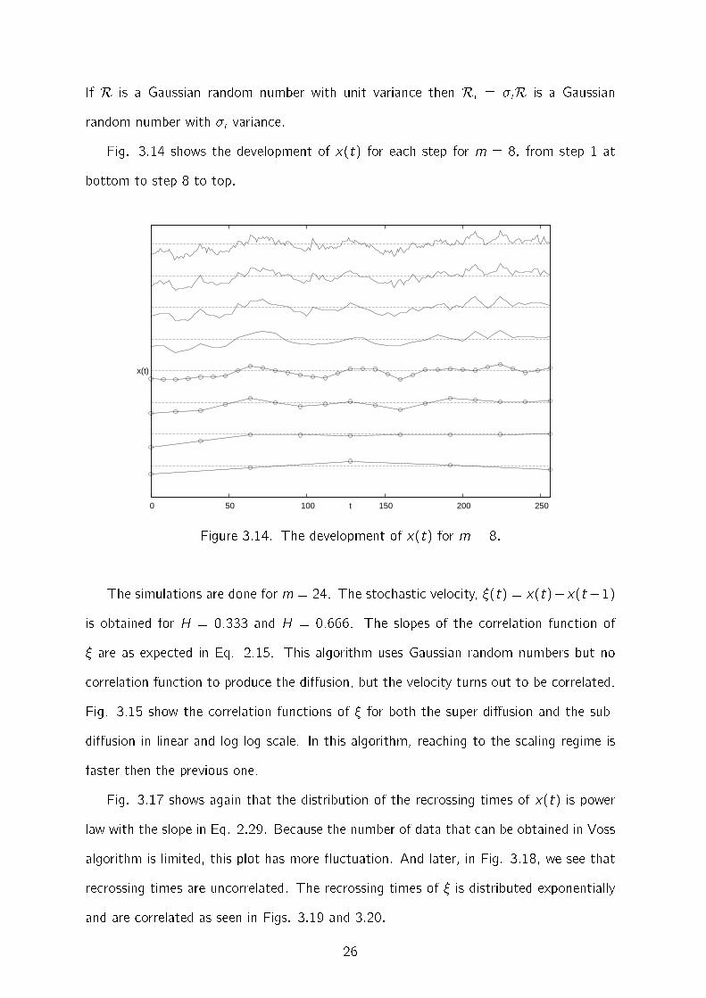
If R is a Gaussian random number with unit variance then Ri = �iR is a Gaussian

random number with �i variance.

Fig. 3.14 shows the development of x(t) for each step for m = 8, from step 1 at

bottom to step 8 to top.

0 50 100 150 200 250t

x(t)

Figure 3.14. The development of x(t) for m = 8.

The simulations are done for m = 24. The stochastic velocity, �(t) = x(t)�x(t�1)

is obtained for H = 0:333 and H = 0:666. The slopes of the correlation function of

� are as expected in Eq. 2.15. This algorithm uses Gaussian random numbers but no

correlation function to produce the di�usion, but the velocity turns out to be correlated.

Fig. 3.15 show the correlation functions of � for both the super-di�usion and the sub-

di�usion in linear and log-log scale. In this algorithm, reaching to the scaling regime is

faster then the previous one.

Fig. 3.17 shows again that the distribution of the recrossing times of x(t) is power

law with the slope in Eq. 2.29. Because the number of data that can be obtained in Voss

algorithm is limited, this plot has more uctuation. And later, in Fig. 3.18, we see that

recrossing times are uncorrelated. The recrossing times of � is distributed exponentially

and are correlated as seen in Figs. 3.19 and 3.20.

26

The aging experiment was possible only for the sub-di�usion because there was not

enough number of recrossing times for the super-di�usion. Fig. 3.21 show that there is

renewal aging for H = 1=3.

-0.12

-0.1

-0.08

-0.06

-0.04

-0.02

0

0 20 40 60 80 100

Φ ξ

t

1e-04

0.001

0.01

0.1

1 10 100

Φ ξ

t

Figure 3.15. The correlation functions of the super-di�usion, H = 2=3,

(circles) and the sub-di�usion, H = 1=3, (triangles) for both normal (up-

per) and log-log (lower) scales.

27

1e-09

1e-08

1e-07

1e-06

1e-05

1e-04

0.001

0.01

0.1

1 10 100 1000

σ2

t

-0.5

0

0.5

1

1.5

2

2.5

3

3.5

4

4.5

1 10 100 1000

S-S

0

t

Figure 3.16. Variance (upper) and DE (lower) of the super-di�usion, H =

2=3, (circles) and the sub-di�usion, H = 1=3, (triangles).

28

1e-05

1e-04

0.001

0.01

0.1

1

10 100 1000

ψ(τ)

τ

Figure 3.17. Distributions of recrossing times of x for the super-di�usion,

H = 2=3, (circles) and the sub-di�usion, H = 1=3, (triangles).

-0.2

0

0.2

0.4

0.6

0.8

1

0 20 40 60 80 100

φ(τ)

τ

-0.2

0

0.2

0.4

0.6

0.8

1

0 20 40 60 80 100

φ(τ)

τ

Figure 3.18. The correlation functions of recrossing times of x for the

super-di�usion, H = 2=3, (upper) and the sub-di�usion,H = 1=3, (lower).

29

1e-07

1e-06

1e-05

1e-04

0.001

0.01

0.1

1

0 5 10 15 20 25

ψ ξ(τ

)

τ

Figure 3.19. Distributions of recrossing times of � for the super-di�usion,

H = 2=3, (circles) and the sub-di�usion, H = 1=3, (triangles).

-0.04

-0.02

0

0.02

0.04

0 20 40 60 80 100

φ ξ(τ

)

τ

-0.04

-0.02

0

0.02

0.04

0 20 40 60 80 100

φ ξ(τ

)

τ

Figure 3.20. The correlation functions of recrossing times of � for the

super-di�usion, H = 2=3, (upper) and the sub-di�usion,H = 1=3, (lower).

30

0.01

0.1

1

1 10 100 1000τ

Ψta

Figure 3.21. Aging of the recrossing times of x for the sub-di�usion for

H = 1=3.

31

CHAPTER 4

RANDOM SURFACE GROWTH

The model of ballistic deposition (BD) is a simple way to establish cooperation among

the columns of a growing surface. It can be used as a model for the birth of cooperation

in complex systems. This model will show that the birth of complexity is associated

with both memory and renewal property. (See the RC model of chapter 2.) It generates

memory properties and non-Poisson renewal events. The variable generating memory can

be regarded as the velocity of a particle driven by a bath with the same time scale, and

the variable generating renewal processes is the corresponding di�usional coordinate.

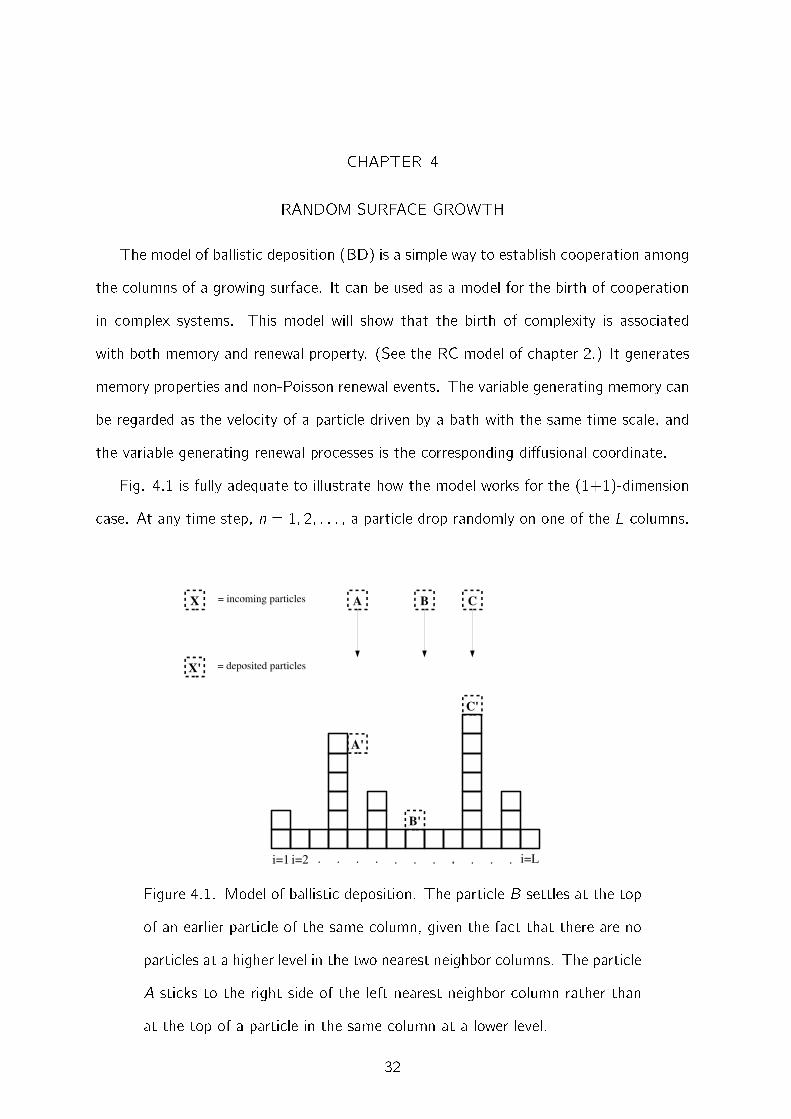
Fig. 4.1 is fully adequate to illustrate how the model works for the (1+1)-dimension

case. At any time step, n = 1; 2; : : : , a particle drop randomly on one of the L columns.

Figure 4.1. Model of ballistic deposition. The particle B settles at the top

of an earlier particle of the same column, given the fact that there are no

particles at a higher level in the two nearest neighbor columns. The particle

A sticks to the right side of the left nearest neighbor column rather than

at the top of a particle in the same column at a lower level.

32

2080

2090

2100

2110

2120

2130

2140

2150

0 100 200 300 400 500 600 700 800 900 1000

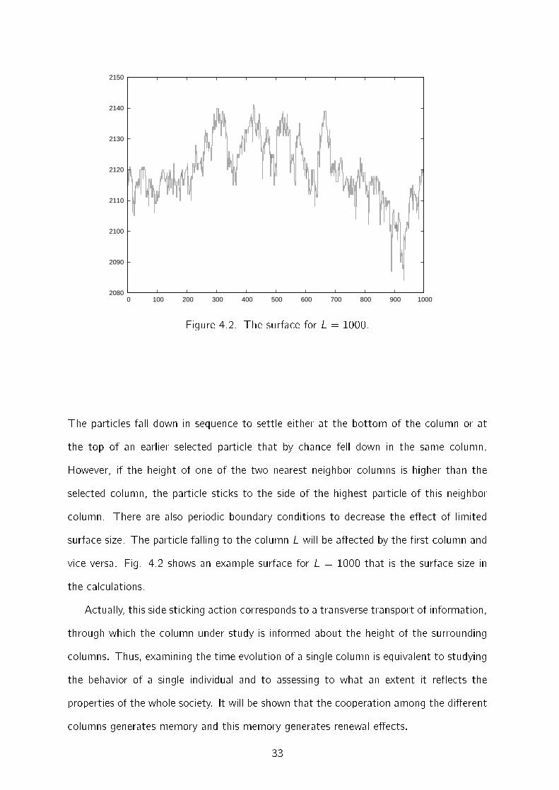
Figure 4.2. The surface for L = 1000.

The particles fall down in sequence to settle either at the bottom of the column or at

the top of an earlier selected particle that by chance fell down in the same column.

However, if the height of one of the two nearest neighbor columns is higher than the

selected column, the particle sticks to the side of the highest particle of this neighbor

column. There are also periodic boundary conditions to decrease the e�ect of limited

surface size. The particle falling to the column L will be a�ected by the �rst column and

vice versa. Fig. 4.2 shows an example surface for L = 1000 that is the surface size in

the calculations.

Actually, this side sticking action corresponds to a transverse transport of information,

through which the column under study is informed about the height of the surrounding

columns. Thus, examining the time evolution of a single column is equivalent to studying

the behavior of a single individual and to assessing to what an extent it re ects the

properties of the whole society. It will be shown that the cooperation among the di�erent

columns generates memory and this memory generates renewal e�ects.

33

4.1. Collective Properties

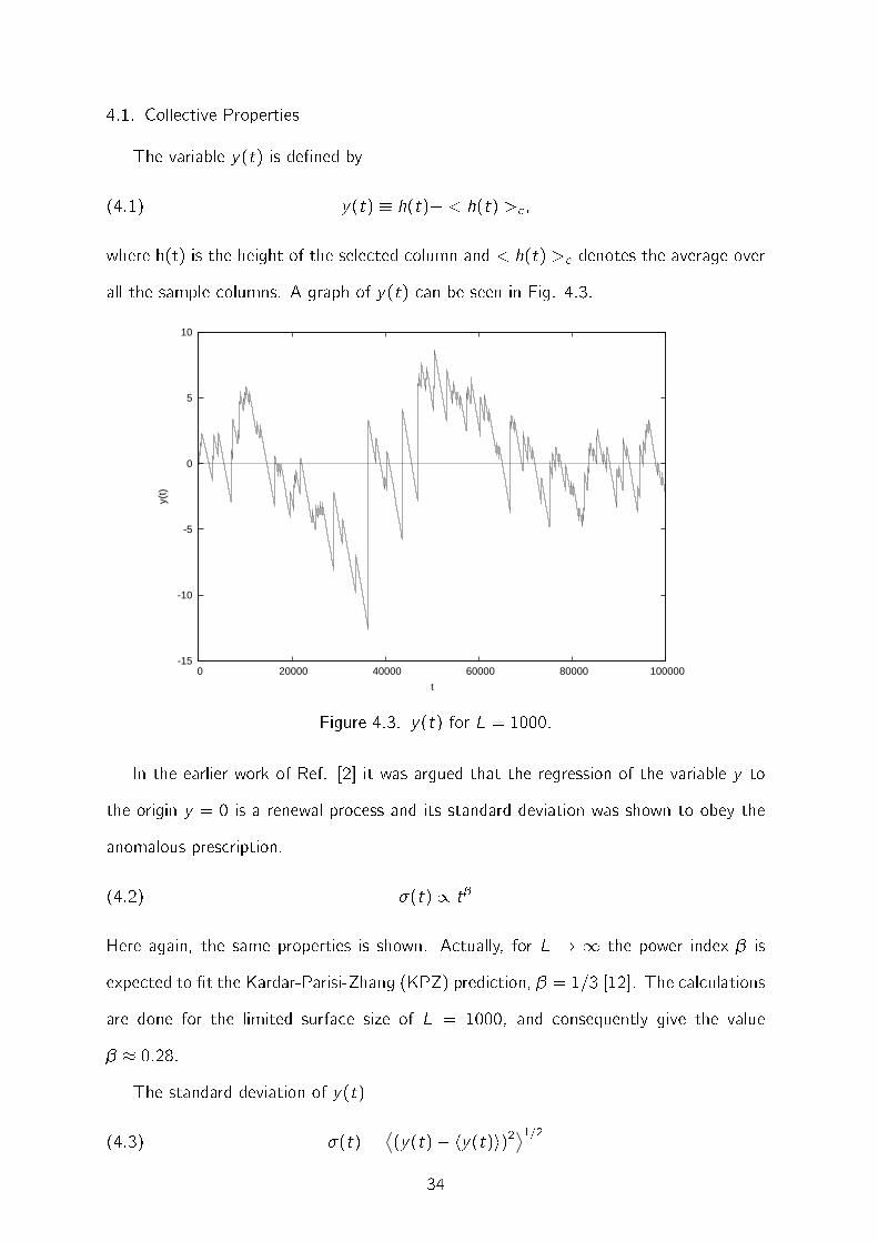
The variable y(t) is de�ned by

(4.1) y(t) � h(t)� < h(t) >c ;

where h(t) is the height of the selected column and < h(t) >c denotes the average over

all the sample columns. A graph of y(t) can be seen in Fig. 4.3.

-15

-10

-5

0

5

10

0 20000 40000 60000 80000 100000

y(t)

t

Figure 4.3. y(t) for L = 1000.

In the earlier work of Ref. [2] it was argued that the regression of the variable y to

the origin y = 0 is a renewal process and its standard deviation was shown to obey the

anomalous prescription.

(4.2) �(t) / t�

Here again, the same properties is shown. Actually, for L ! 1 the power index � is

expected to �t the Kardar-Parisi-Zhang (KPZ) prediction, � = 1=3 [12]. The calculations

are done for the limited surface size of L = 1000, and consequently give the value

� � 0:28.

The standard deviation of y(t)

(4.3) �(t) =⟨

(y(t)� hy(t)i)2⟩1=2

34

1

10

1000 10000 100000 1e+06 1e+07 1e+08

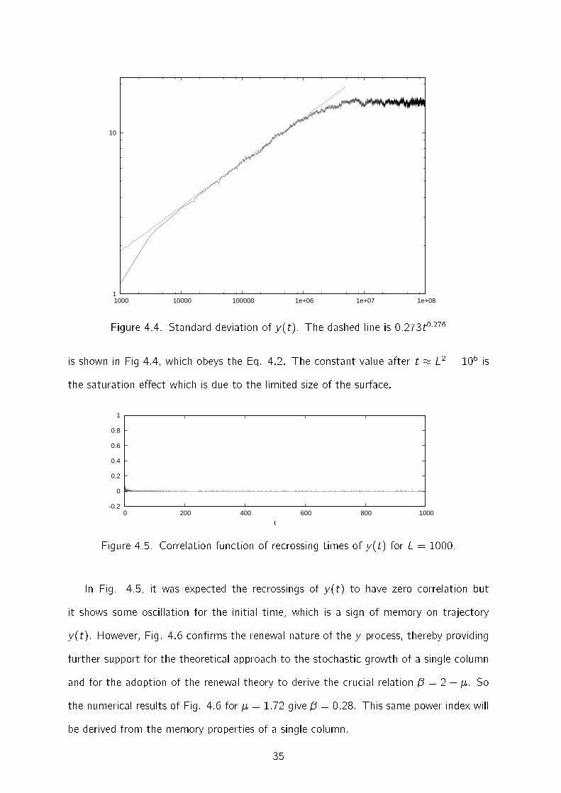
Figure 4.4. Standard deviation of y(t). The dashed line is 0:273t0:276

is shown in Fig 4.4, which obeys the Eq. 4.2. The constant value after t � L2 = 106 is

the saturation e�ect which is due to the limited size of the surface.

-0.2

0

0.2

0.4

0.6

0.8

1

0 200 400 600 800 1000

t

Figure 4.5. Correlation function of recrossing times of y(t) for L = 1000.

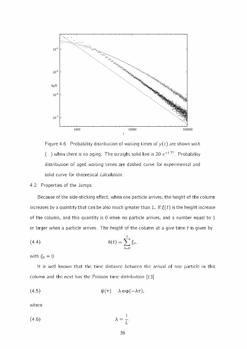
In Fig. 4.5, it was expected the recrossings of y(t) to have zero correlation but

it shows some oscillation for the initial time, which is a sign of memory on trajectory

y(t). However, Fig. 4.6 con�rms the renewal nature of the y -process, thereby providing

further support for the theoretical approach to the stochastic growth of a single column

and for the adoption of the renewal theory to derive the crucial relation � = 2 � �. So

the numerical results of Fig. 4.6 for � = 1:72 give � = 0:28. This same power index will

be derived from the memory properties of a single column.

35

10-7

10-6

10-5

10-4

1000 10000 100000

t

ψa(t)

Figure 4.6. Probability distribution of waiting times of y(t) are shown with

(+) when there is no aging. The straight solid line is 20 x�1:72. Probability

distribution of aged waiting times are dashed curve for experimental and

solid curve for theoretical calculation.

4.2. Properties of the Jumps

Because of the side-sticking e�ect, when one particle arrives, the height of the column

increases by a quantity that can be also much greater than 1. If �(t) is the height increase

of the column, and this quantity is 0 when no particle arrives, and a number equal to 1

or larger when a particle arrives. The height of the column at a give time t is given by

(4.4) h(t) =t∑n=0

�n;

with �0 = 0.

It is well known that the time distance between the arrival of one particle in this

column and the next has the Poisson time distribution [13]

(4.5) (�) = � exp(���);

where

(4.6) � =1L:

36

10-8

10-7

10-6

10-5

10-4

10-3

10-2

10-1

1

1 10 100 1000 10000

t

ψ

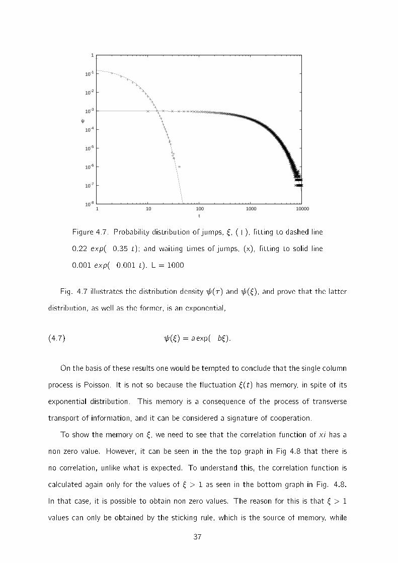
Figure 4.7. Probability distribution of jumps, �, (+), �tting to dashed line

0:22 exp(�0:35 t); and waiting times of jumps, (x), �tting to solid line

0:001 exp(�0:001 t). L = 1000

Fig. 4.7 illustrates the distribution density (�) and (�), and prove that the latter

distribution, as well as the former, is an exponential,

(4.7) (�) = a exp(�b�):

On the basis of these results one would be tempted to conclude that the single column

process is Poisson. It is not so because the uctuation �(t) has memory, in spite of its

exponential distribution. This memory is a consequence of the process of transverse

transport of information, and it can be considered a signature of cooperation.

To show the memory on �, we need to see that the correlation function of xi has a

non-zero value. However, it can be seen in the the top graph in Fig 4.8 that there is

no correlation, unlike what is expected. To understand this, the correlation function is

calculated again only for the values of � > 1 as seen in the bottom graph in Fig. 4.8.

In that case, it is possible to obtain non-zero values. The reason for this is that � > 1

values can only be obtained by the sticking rule, which is the source of memory, while

37

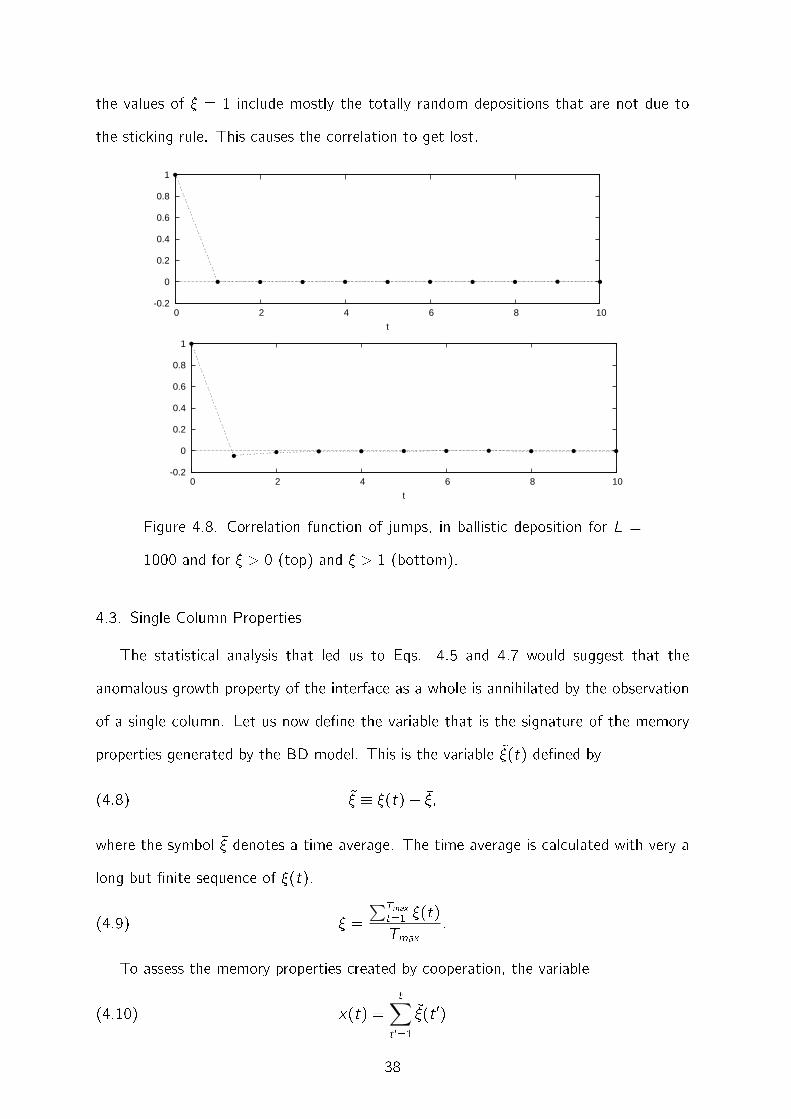
the values of � = 1 include mostly the totally random depositions that are not due to

the sticking rule. This causes the correlation to get lost.

-0.2

0

0.2

0.4

0.6

0.8

1

0 2 4 6 8 10

t

-0.2

0

0.2

0.4

0.6

0.8

1

0 2 4 6 8 10

t

Figure 4.8. Correlation function of jumps, in ballistic deposition for L =

1000 and for � > 0 (top) and � > 1 (bottom).

4.3. Single Column Properties

The statistical analysis that led us to Eqs. 4.5 and 4.7 would suggest that the

anomalous growth property of the interface as a whole is annihilated by the observation

of a single column. Let us now de�ne the variable that is the signature of the memory

properties generated by the BD model. This is the variable ~�(t) de�ned by

(4.8) ~� � �(t)� ��;

where the symbol �� denotes a time average. The time average is calculated with very a

long but �nite sequence of �(t).

(4.9) �� =∑Tmax

t=1 �(t)Tmax

:

To assess the memory properties created by cooperation, the variable

(4.10) x(t) =t∑

t 0=1

~�(t 0)

38

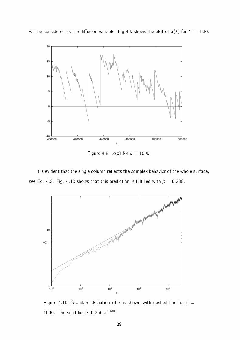
will be considered as the di�usion variable. Fig 4.9 shows the plot of x(t) for L = 1000.

-10

-5

0

5

10

15

20

400000 420000 440000 460000 480000 500000

t

Figure 4.9. x(t) for L = 1000.

It is evident that the single column re ects the complex behavior of the whole surface,

see Eq. 4.2. Fig. 4.10 shows that this prediction is ful�lled with � = 0:288.

1

10

107106105104103

t

w(t)

Figure 4.10. Standard deviation of x is shown with dashed line for L =

1000. The solid line is 0:256 x0:288

39

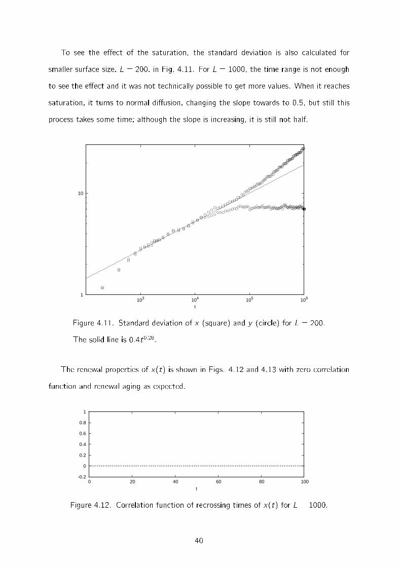
To see the e�ect of the saturation, the standard deviation is also calculated for

smaller surface size, L = 200, in Fig, 4.11. For L = 1000, the time range is not enough

to see the e�ect and it was not technically possible to get more values. When it reaches

saturation, it turns to normal di�usion, changing the slope towards to 0:5, but still this

process takes some time; although the slope is increasing, it is still not half.

1

10

106105104103

t

Figure 4.11. Standard deviation of x (square) and y (circle) for L = 200.

The solid line is 0:4t0:28.

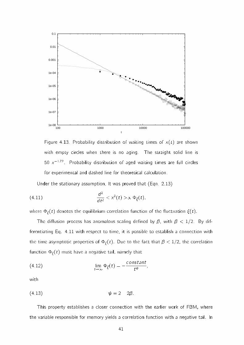
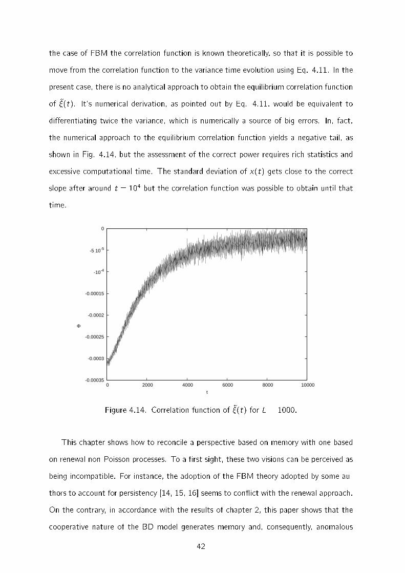
The renewal properties of x(t) is shown in Figs. 4.12 and 4.13 with zero correlation

function and renewal aging as expected.

-0.2

0

0.2

0.4

0.6

0.8

1

0 20 40 60 80 100

t

Figure 4.12. Correlation function of recrossing times of x(t) for L = 1000.

40

1e-08

1e-07

1e-06

1e-05

1e-04

0.001

0.01

0.1

100 1000 10000 100000

t

Figure 4.13. Probability distribution of waiting times of x(t) are shown

with empty circles when there is no aging. The straight solid line is

50 x�1:72. Probability distribution of aged waiting times are full circles

for experimental and dashed line for theoretical calculation.

Under the stationary assumption, It was proved that (Eqn. 2.13)

(4.11)d2

dt2 < x2(t) >/ �~�(t);

where �~�(t) denotes the equilibrium correlation function of the uctuation �(t).

The di�usion process has anomalous scaling de�ned by �, with � < 1=2. By dif-

ferentiating Eq. 4.11 with respect to time, it is possible to establish a connection with

the time asymptotic properties of �~�(t). Due to the fact that � < 1=2, the correlation

function �~�(t) must have a negative tail, namely that

(4.12) limt!1�~�(t) = �constant

t ;

with

(4.13) = 2� 2�:

This property establishes a closer connection with the earlier work of FBM, where

the variable responsible for memory yields a correlation function with a negative tail. In

41

the case of FBM the correlation function is known theoretically, so that it is possible to

move from the correlation function to the variance time evolution using Eq. 4.11. In the

present case, there is no analytical approach to obtain the equilibrium correlation function

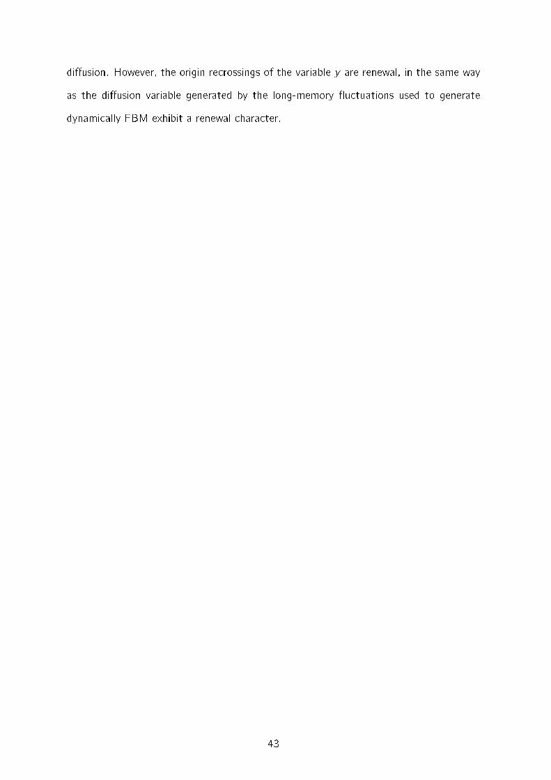
of ~�(t). It's numerical derivation, as pointed out by Eq. 4.11, would be equivalent to

di�erentiating twice the variance, which is numerically a source of big errors. In, fact,

the numerical approach to the equilibrium correlation function yields a negative tail, as

shown in Fig. 4.14, but the assessment of the correct power requires rich statistics and

excessive computational time. The standard deviation of x(t) gets close to the correct

slope after around t = 104 but the correlation function was possible to obtain until that

time.

-0.00035

-0.0003

-0.00025

-0.0002

-0.00015

-10-4

-5 10-5

0

0 2000 4000 6000 8000 10000

t

Φ

Figure 4.14. Correlation function of ~�(t) for L = 1000.

This chapter shows how to reconcile a perspective based on memory with one based

on renewal non-Poisson processes. To a �rst sight, these two visions can be perceived as

being incompatible. For instance, the adoption of the FBM theory adopted by some au-

thors to account for persistency [14, 15, 16] seems to con ict with the renewal approach.

On the contrary, in accordance with the results of chapter 2, this paper shows that the

cooperative nature of the BD model generates memory and, consequently, anomalous

42

di�usion. However, the origin recrossings of the variable y are renewal, in the same way

as the di�usion variable generated by the long-memory uctuations used to generate

dynamically FBM exhibit a renewal character.

43

CHAPTER 5

TRAJECTORY AND DENSITY MEMORY

This chapter discusses the connection between trajectory and density memory. The

�rst form of memory is a property of a stochastic trajectory, whose stationary correlation

function shows that the uctuation at a given time depends on the earlier uctuations.

The density memory is a property of a collection of trajectories, whose density time evo-

lution is described by a time convoluted equation showing that the density time evolution

depends on its past history. It will be shown that the trajectory memory does not nec-

essarily yield density memory, and that density memory might be compatible with the

existence of abrupt jumps resetting to zero the system's memory.

In literature it seems to be widely accepted that density and trajectory memory are

equivalent. However, there are good reasons to not share this conviction. In the last few

years, there has been an increasing interest for the di�usion equations emerging from

the perspective of continuous time random walk (CTRW) [27]. Since the fundamental

work of Kenkre, Shlesinger and Montroll [28], it is well known that the CTRW generates,

for the time evolution of density, the same time convoluted structure as the methods of

Refs. [17, 18, 23, 24]. According to the earlier de�nitions, this is density memory, and

the expected equivalence between trajectory and density memory is clearly violated, if we

keep in mind that the CTRW is a process based on jumps, whose occurrence resets to

zero the system's memory. To make this aspect more evident, the derivation of CTRW

from the di�usion equation will be shown in Section 5.1:

(5.1)@@tp(x; t) = D

∫ t

0d��(�)

@2

@x2p(x; t � �):

Eq.5.1 has the earlier mentioned time convoluted structure, thereby implying that the

time evolution of the probability density p(x; t) depends on the earlier times t � � : this

explains why it is called density memory. What about trajectory memory? As earlier

44

pointed out, there is no such memory here, due to the occurrence of memory erasing

jumps.

Now, let us point out another aspect con icting with the naive conviction that tra-

jectory and density memory are equivalent. Let us go back to the chapter 2 of FBM, or,

more precisely, to the dynamic approach to FBM, to generate the following generalized

di�usion equation

(5.2)@@tp(x; t) = D

(∫ t

0d��(�)

)@2

@x2p(x; t):

Note that the function �(t) in this case is the correlation function of �, and it has

fat tails, indicating the existence of trajectory memory. Yet, the di�usion equation does

not have the time convoluted structure of Eq. 5.1. The work of Ref. [31] shows that

the emergence of the time-convolutionless structure of Eq. 5.2, to compare to the

time-convolution structure of Eq. 5.1, is determined by the fact that the stochastic

variable �(t) is Gaussian in the case of Eq. 5.2. In the recent work of Ref. [32] Kenkre

noticed that, although the two equations might yield the same second moment, the

higher moments are not identical and that Eq. 5.2 cannot produce the transition from

merely di�usive to merely wave-like motion, whereas Eq. 5.1 does.

The main purpose here is to shed some light into the confusion concerning the re-

lations between these two kinds of memory. The solution of the very elusive problem

of establishing the trajectory properties behind Eq. 5.1, when this equation generates

super-di�usion, will also be shown. The trajectory properties of this equation are well

known in the sub-di�usional case [33], but in the super-di�usion case its correct interpre-

tation in terms of CTRW does not exist [34] and there are good reasons to believe that

in this case Eq. 5.1 is incompatible with a CTRW origin. In line with [34], the trajectory

memory picture that explains the dynamical origin of Eq. 5.1 in the super-di�usion case

will be studied.

45

5.1. The Generalized Di�usion Equation from the CTRW Perspective

This process can be simply described by a particle doing random jumps to left or right.

In one dimension, the equation of motion is

(5.3)ddtx = �;

where � is +1 or �1 randomly and time is discrete. Let us imagine a sequel of events

described by

(5.4) p(n) = Mnp(0):

The symbol p denotes a vector with in�nite components pi �tting the normalization

condition

(5.5)1∑

i=�1pi = 1:

The initial condition is when at n = 0, only the site i = 0 is occupied and all the other

sites are empty. At each time step the particle makes a transition from the site i = 0 to

other sites, depending on the form of the matrix M. In this paper, M has the following

speci�c form

(5.6) M �∑ 12

(ji >< i + 1j+ ji + 1 >< i j):

The choice of this quantum-like formalism is done to avoid the cumbersome matrix

notation, and it does not imply any departure from the classical condition. For instance,

since at t = 0 only the site i = 0 is occupied,

(5.7) Mp(0) = Mj0 >=12

(j1 > + < �1j);

which means that the particle at the �rst step will jump with equal probability from the

site i = 0 to the two nearest neighbor sites j1 > and j � 1 >. It should be easy to

consider transition matrices with a di�erent form.

For an individual trajectory, the position x(n) of the particle after n steps will be

(5.8) x(n) =n∑

i

�i :

46

The time distance between two consecutive jumps is �xed and equal to tu. The spatial

distance between two nearest neighbor sites is �xed and is equal to a.

Let us do the experiment with many particles, moving from the same initial site i = 0.

The position x(n) will correspond to a given site with index i . Let us count how many

particles are found in this site and call ni the number of particles occupying this site, and

we divide this number by the total number of trajectories, N. This will give the relation

(5.9)niN

= pi(n) =< i jMnjp(0) > :

With this equivalence between stochastic trajectories and a probabilistic description

in mind, the �rst conclusion is that Eq. 5.9 represents the probability distribution of this

set of random walkers at a given time t = ntu. In accordance with the central limit

theorem, the distribution of x is Gaussian. In this condition, standard deviation is

(5.10) < x2(n) >1=2/ n1=2

and the di�usion equation is

(5.11)@@np(x; n) = D

@2

@x2p(x; n);

which gives the ordinary di�usion.

It is assumed that tu is the minimum possible time, and that the experimental time t is

much larger than tu. Let us now make also the crucial assumption that the time distance

between the occurrence of the nth event, occurring at time tn, and the occurrence of the

(n+ 1)th event, occurring at time tn+1, rather than being �xed, uctuates. The assump-

tion that the time distance between two nearest neighbor events uctuates is physically

plausible. In fact, if the ordinary di�usion generating uctuations are a consequence of

the collision between the particle of interest and the bath molecules, it is reasonable that

these collisions do not occur at regular but at erratic times. Thus the quantity

(5.12) �n = tn+1 � tn

is a stochastic variable with the distribution density (�).

47

The vector p(t) is related to the vector p(0) by means of

(5.13) p(t) =1∑n=0

∫ t

0 n(�)(t � �)Mnp(0)d�:

Note that the function n(t) denotes the probability density for a sequel of n event to

occur, the last of which occurs exactly at t. Due to the statistical independence of these

events (App. G), the Laplace transform of n(t) is ( (u))n, with (u) denoting the

Laplace transform of (t) � 1(t), namely the probability density for one event to occur

at time t. The function (t) is the probability that no event occurs up to time t, and

it is de�ned by

(5.14) (t) �∫ 1

tdt 0 (t 0):

The physical meaning of Eq. 5.13 is made evident by the following remarks. The speci�c

state p(t) is determined by the last of a sequel of collisions occurring prior to time t.

The number of collisions is arbitrary, thereby explaining the index n running from 0 to

1. No further event occurs between � and t. This is taken into account by multiplying

n(�) by (t � �).

It is a straightforward to prove that Eq. 5.13 is equivalent to (App. J)

(5.15)@@t

p(t) = �∫ t

0d��(�)Kp(t � �);

with

(5.16) K = 1�M:

The memory kernel �(t) is related to (t) in the Laplace domain through

(5.17) �(u) =u (u)

1� (u):

These results are obtained by comparing the Laplace transform of Eq. 5.15 to the Laplace

transform of Eq. 5.13.

With the choice of Eq. 5.6, the result of Eq. 5.15 can be expressed in a form

equivalent to that proposed by Kenkre and Knox in Ref. [35]. In fact, if the choice of

48

Eq. 5.6 applies, it becomes

(5.18) �Kpji = �(1�M)pji = �pi +pi+1

2+pi�1

2=

12@2

@x2p(x; t):

Thus, Eq. 5.15 is rewritten as follows

(5.19)@@tp(x; t) = D

∫ t

0d��(�)

@2

@x2p(x; t � �):

Notice that if the value a is assigned to the distance between the nearest neighbor sites

of the model here under discussion, the di�usion coe�cient D reads D = a2=2.

It is worth mentioning that the GDE of Eq. 5.19 drives the density of the di�usion

process described by

(5.20)ddtx(t) = �R(t);

where �R(t) is a uctuation almost always vanishing but in the correspondence of a

collision, where it takes the value 1 or �1, according to the coin tossing prescription.

The di�usion equation of Eq. 5.19 in the time asymptotic limit yields scaling. This

means:

(5.21) p(x; t) =1t�F (xt�

);

with � called scaling coe�cient, and F (y) being a function of y , di�erent in general from

a Gaussian function. This is a formal but rigorous way of assessing that in the time

asymptotic condition x / t�. The deviation from ordinary di�usion is signaled by � 6= 0:5

and/or F (y) departing from the Gaussian form.

It is evident that the departure from ordinary di�usion, when it occurs, takes the form

of sub-di�usion, namely, with � < 0:5: this is so because the longer the recrossing time

in one site, the slower the di�usion process. To make the recrossing in one site as long

as possible, set

(5.22) (�) = (�� 1)T ��1

(� + T )�;

with the power index � meeting the condition

49

(5.23) 1 < � < 2;

so that the mean recrossing time in one site is in�nite.

To evaluate the scaling in the case of Eq. 5.19 it is convenient to study the Fourier-

Laplace transform of p(x; t), with k and u being the variables conjugated to x and t,

respectively. The Fourier-Laplace transform of p(x; t) is denoted p(k; u). Its explicit

form is

(5.24) p(k; u) =1

u + k2D�(u):

Using Eq. 5.17 and the limiting condition u ! 0 of (�) of Eq. 5.22 as in App. H,

when the condition of Eq. 5.23 applies,

(5.25) (u) = 1� �(2� �)(uT )��1;

we obtain

(5.26) p(k; u) =1

u + k2u2��D�(2��)

:

To determine the unknown scaling coe�cient �, let us set k / u� and plug it into Eq.

5.26. The value of � making p(u�; u) proportional to 1=u is

(5.27) � =(�� 1)

2;

which is in fact smaller than 1=2, when condition (5.23) applies.

5.2. Auxiliary Fluctuation

In this section, the memoryless trajectories behind Eq. 5.1, namely, the time con-

voluted di�usion equation generated by the CTRW perspective will be illustraded. The

hypothesis of instantaneous collision made in Section 5.1 is not essential to generate

the sub-di�usional process there described. To double check the theoretical arguments

by means of numerical simulation, it is convenient to adopt a uctuation with the time

50

interval between two consecutive renewal events �lled with auxiliary events. This uctu-

ation is called �A(t). This section is devoted to illustrating a dynamic model producing

this kind of uctuation.

Let us imagine a particle with coordinate y , moving within the interval I � [0; 1],

with the following equation of motion (App.K)

(5.28)ddty = �y z ;

with z � 1, and 0 < � << 1. When the particle reaches the border, y = 1, is injected

back to a new initial condition y0, with uniform probability, it is easy to prove [40, 41]

that the waiting time distribution is given by (5.22) with

(5.29) � =z

(z � 1):

Let us now de�ne a uctuation �A(t) as follows. From time t = 0 to time �1,

corresponding to the particle reaching the border, the uctuation �A(t) is identical to the

velocity dy=dt of the particle, with a sign � depending on the coin tossing prescription,

namely,

(5.30) �A(t) = R �y�=(��1)0[

1� y 1=(��1)0

�(��1)t

]� ;

where y0 is a random number of the interval I and R is �1 randomly. This means that

the system is prepared in such a way that at time t = 0 all the systems of the ensemble

are at the beginning of the deterministic dynamic process, at the end of which a new

back injection will occur. Of course y0 is selected randomly, with uniform distribution

within the interval I. Thus, the time of the second back injection changes from system

to system, and the probability of the �rst sojourn time, �1, is given by Eq. 5.22. From

time t = �1, corresponding to the �rst jump after preparation to time t = �1 + �2, at

which the second jump occurs, the uctuation �(t) goes as follows:

51

(5.31) �A(t) = R �y�=(��1)1[

1� y 1=(��1)1

�(��1) (t � �1)

]� ;

where y1 denotes the initial condition after the �rst back injection, again selected ran-

domly with uniform probability in the interval I, and so on.

-0.01

-0.008

-0.006

-0.004

-0.002

0

0.002

0.004

0.006

0.008

0.01

0 500 1000 1500 2000 2500 3000 3500 4000 4500 5000

t

Figure 5.1. Auxiliary uctuation �A(t) for � = 1:666 and � = 0:01.

-4

-3.5

-3

-2.5

-2

-1.5

-1

-0.5

0

0.5

1

0 500 1000 1500 2000 2500 3000 3500 4000 4500 5000

t

Figure 5.2. Plot of the motion in Eq. 5.32 for � = 1:666 and � = 0:01.

Let us focus now our attention on the di�usion process described by

(5.32)ddtx(t) = �A(t):

Figs. 5.1 and 5.2 show example functions x(t) and �A(t). In this case, it is expected that

the uctuation �A(t) will produce a sub-di�usion process with the anomalous scaling of

Eq. (5.27) with � meeting the condition of (5.23).

Let us explain the intuitive reasons that lead us to make the prediction of Eq. (5.27).

As explained by the arguments of Section 5.1, the generalized di�usion equation of Eq.

52

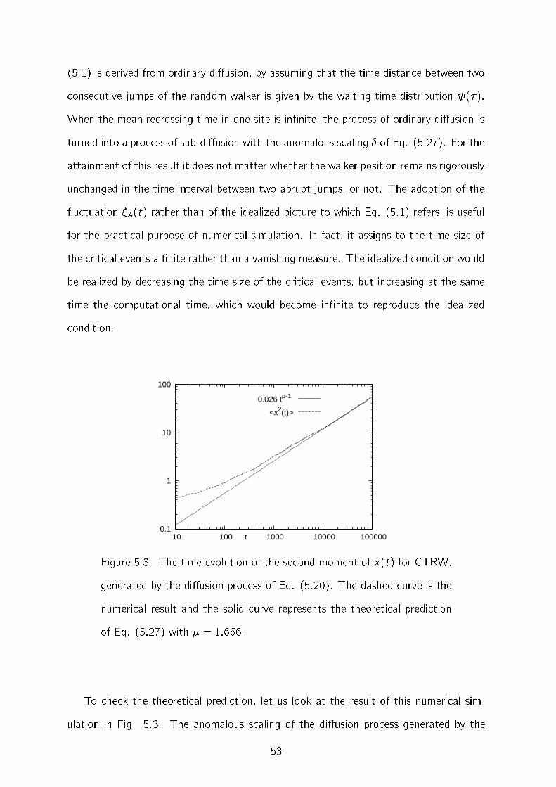
(5.1) is derived from ordinary di�usion, by assuming that the time distance between two

consecutive jumps of the random walker is given by the waiting time distribution (�).

When the mean recrossing time in one site is in�nite, the process of ordinary di�usion is

turned into a process of sub-di�usion with the anomalous scaling � of Eq. (5.27). For the

attainment of this result it does not matter whether the walker position remains rigorously

unchanged in the time interval between two abrupt jumps, or not. The adoption of the

uctuation �A(t) rather than of the idealized picture to which Eq. (5.1) refers, is useful

for the practical purpose of numerical simulation. In fact, it assigns to the time size of

the critical events a �nite rather than a vanishing measure. The idealized condition would

be realized by decreasing the time size of the critical events, but increasing at the same

time the computational time, which would become in�nite to reproduce the idealized

condition.

0.1

1

10

100

10 100 1000 10000 100000t

0.026 tµ-1

<x2(t)>

Figure 5.3. The time evolution of the second moment of x(t) for CTRW,

generated by the di�usion process of Eq. (5.20). The dashed curve is the

numerical result and the solid curve represents the theoretical prediction

of Eq. (5.27) with � = 1:666.

To check the theoretical prediction, let us look at the result of this numerical sim-

ulation in Fig. 5.3. The anomalous scaling of the di�usion process generated by the

53

uctuation �A(t) is evaluated through the second moment of the probability distribu-

tion density, which shows that, in the asymptotic limit, the numerical scaling becomes

identical to the theoretical scaling of Eq. (5.27).

Eq. (5.1), which is an evident expression of density memory emerges from the time

evolution of a bunch of trajectories, with no memory. After a jump, the quantity �A(t)

undergoes a time evolution determined by a random choice of initial condition, with no

memory whatsoever of the time evolution of �A(t) prior to the last jump.

5.3. On the Dynamical Nature of the Memory Kernel of the Ctrw Generalized Di�usion

Equation

This Section shows that the memory kernel �(t) of the generalized di�usion equation

of Eq. (5.1) is not an equilibrium correlation function. Eq. (5.32) gives

(5.33) x(t) =∫ t

0�A(t 0)dt 0:

This means that, as in the earlier section, all the walkers move from x = 0 at t = 0.

The second moment of this di�usion process reads

(5.34) < x(t)2 >=∫ t

0dt 0

∫ t

0dt 00 < �A(t 0)�A(t 00) > :

Since the correlation function of �A is not stationary, the integrand can not be written

in terms of t � t` as in Eq.2.8. By di�erentiating Eq. (5.34) twice with respect to time,

we obtain

(5.35)d2

dt2 < x2(t) >= 2 < �2A(t) > +2

∫ t

0dt 0 ddt

< �A(t)�A(t 0) > :

On the other hand, using Eq. (5.19) (App. L), we get

(5.36)d2

dt2 < x2(t) >= 2D�(t):

By comparing Eq. (5.35) to Eq. (5.36) we arrive at the important equality

(5.37) D�(t) =< �2A(t) > +

∫ t

0dt 0 ddt

< �A(t)�A(t 0) > :

54

This relation shows that �(t) is not a correlation function. �(t) is related to a true

correlation function, < �A(t)�A(t 0) >, by a functional relation, and the true correlation

function is not stationary.

Let us try to �nd the functional form of the memory kernel, �(t). As shown in

Section 5.2, all the systems of the Gibbs ensemble are prepared in the condition where

�(0) = y�=(��1)0 , where y0 is the initial random position. After this initial value, which is

equivalent to the condition created by a jump occurring at t = 0, a long time is required

to meet again another jump. Let us discuss here the ideal condition where the time

interval between two signi�cant uctuations is really empty. To �ll it, in�nitely many

other trajectories must be generated to produce signi�cant uctuations in this empty

time interval. In the book of Feller [42] (see also Ref. [43]), it is shown that the density

of events goes as t2��, which gives

(5.38) < �2A(t) >=

C(t + T )2�� ;

and

(5.39) < �A(t)�A(t 0) >=C

(t + T )2��F (t � t 0);

respectively. With some algebra (App. M), we �nd

(5.40) D�(t) = �(2� �)CF (0)(T + t)3�� +

C(T + t)2��F (t):

The adoption of fractional [47, 48] rather than integer derivatives is becoming more

and more popular to address the study of complex systems. An interesting recent example

is given by the work of Sokolov and KlafterRef in [33]. It is written here with a notation

change so as to make it easier to see the connection with the other results.

(5.41)@@tp(x; t) =

1�(2� �)

ddt

∫ t

0d�

1(t � �)2��

@2

@x2p(x; �);

with the power index � meeting the condition of Eq. 5.23. The term on the right-

hand side of this equation can be expressed by means of the Riemann-Liouville fractional

55

derivative [47, 48] de�ned in general by

(5.42)d�

dt�f (t) =

1�(n � �)

dn

dtn

∫ t

0(t � t 0)n���1f (t 0)dt 0;

with n being the smallest integer exceeding �. With this de�nition, Eq. 5.41 reads

(5.43)@@tp(x; t) =

�(�)�(2� �)

d1��dt1��

@2

@x2p(x; t);

with � = �� 1.

The authors of Ref. [33] found the interesting result that the same di�usion process

can be expressed by means of

(5.44)@�

@t�p(x; t) =

@2

@x2p(x; t);

provided that use is made of the Caputo fractional derivative, advocated by Mainardi

[47, 48], de�ned by

(5.45)d�

dt�f (t) =

1�(n � �)

∫ t

0(t � t 0)n���1 d

n

dtnf (t 0)dt 0:

Sokolov and Klafter [33] compare their GDE to the GDE of Kenkre and Knox [35],

which is formally identical to Eq. 5.19, and point out as striking di�erence between this

equation and the equation proposed by Kenkre and Knox [35] the additional time deriv-

ative in the front of the integral. Actually, their equation is equivalent to the generalized

master equation of Eq. 5.15 and the additional time derivative has a physical meaning

that will be properly explained.

For this purpose, let us write again Eq.5.41 in the slightly di�erent form

(5.46)@@tp(x; t) =

1�(2� �)

ddt

∫ t

0d�

1(T + t � �)2��

@2

@x2p(x; �);

with T denoting a time interval that will be to sent to zero at a given phase of this

discussion. By di�erentiating with respect to time, Eq. 5.46 is written in the following

form

@@tp(x; t) =

1�(2� �)T 2��

@2

@x2p(x; t)(5.47)

� (2� �)�(2� �)

∫ t

0d�

1(T + t � �)3��

@2

@x2p(x; �):

56

This means that this result can be obtained from Eq. 5.15 and so from the form of

Kenkre and Knox [35] by adopting for the memory kernel �(t) the following expression

(5.48) D�(t) =�(t)

�(2� �)T 2�� � (2� �)�(2� �)

1(T + t)3�� :

A complete equivalence with the fractional derivative perspective is established by

assuming

(5.49)C

(T + t)2��F (t) =�(t)

�(2� �)T 2�� :

This is equivalent to assuming that the the decay of F (t)=(T + t)2�� is signi�cantly

faster that 1=t3��.

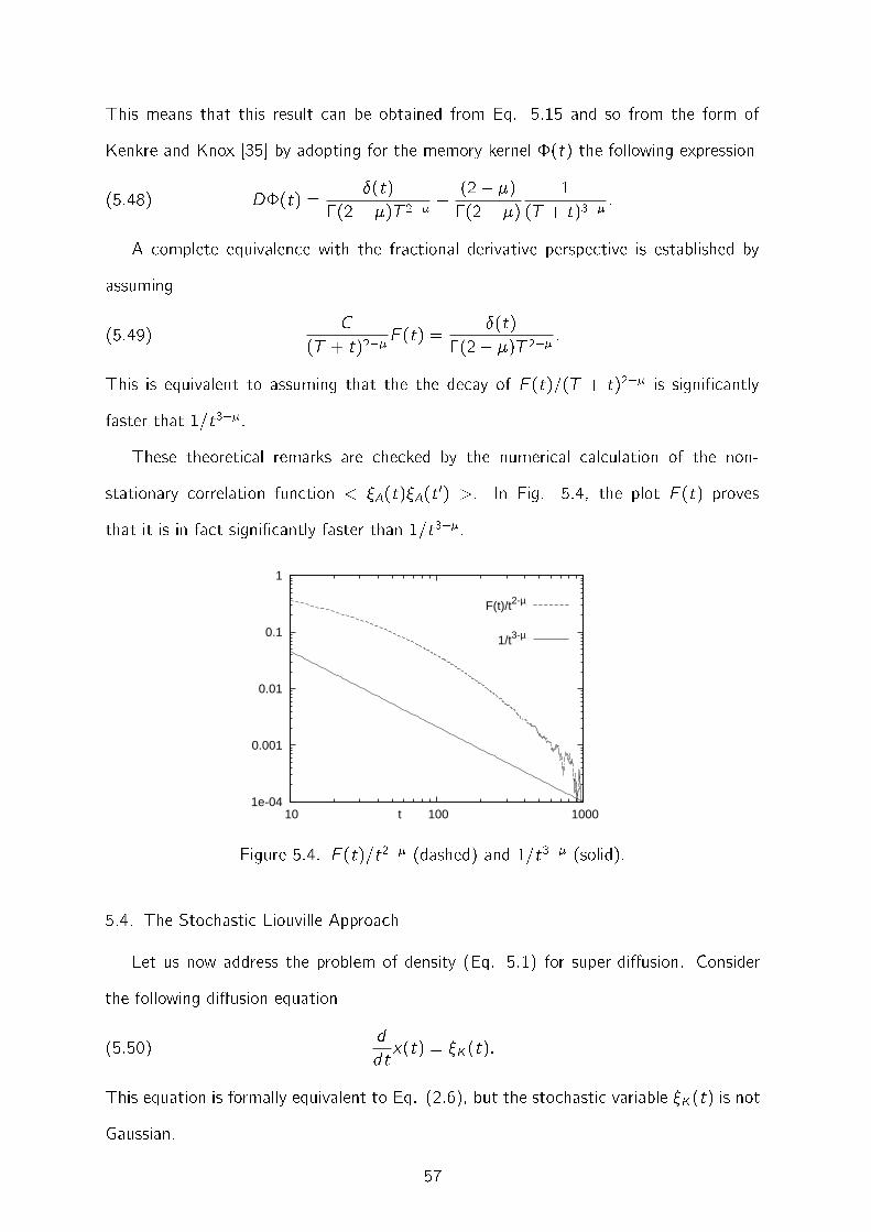
These theoretical remarks are checked by the numerical calculation of the non-

stationary correlation function < �A(t)�A(t 0) >. In Fig. 5.4, the plot F (t) proves

that it is in fact signi�cantly faster than 1=t3��.

1e-04

0.001

0.01

0.1

1

10 100 1000t

F(t)/t2-µ

1/t3-µ

Figure 5.4. F (t)=t2�� (dashed) and 1=t3�� (solid).

5.4. The Stochastic Liouville Approach

Let us now address the problem of density (Eq. 5.1) for super-di�usion. Consider

the following di�usion equation

(5.50)ddtx(t) = �K(t):

This equation is formally equivalent to Eq. (2.6), but the stochastic variable �K(t) is not

Gaussian.

57

Let us adopt the Liouville formalism and let us write the time evolution of the total

probability density �(x; �K; t) as follows

(5.51)ddt�(x; �K; t) = LT�(x; �K; t) �

{��K ddx + LB

}�(x; �K; t):

The operator LB is responsible for the time evolution of the probability density of �K,

namely, it is a bath operator. Following the stochastic Liouville approach of Kubo [36,

37, 38], let us consider the density �(x; �K; t) as a vector state to expand in the basis

set of the eigenstates of LB. In the stationary case the bath operator must have an

eigenstate j0 > with vanishing eigenvalue,

(5.52) LBj0 >= 0:

From within this quantum-like formalism, the out-of-equilibrium properties of the bath

must be taken into account. The non-equilibrium eigenstates j� >, with � 6= 0, are

de�ned by

(5.53) LBj� >= i!�j� > :

With no loss of generality, let us assume

(5.54) !�� = �!�

and

(5.55) j� >= j!� >= j! > :

The variable �K becomes the operator de�ned by

(5.56) �Kj0 >=∑

� 6=0

K�j� >; �Kj� >= j0 >

and the probabilities are set as

(5.57) p0(x; t) �< 0j�(x; �K; t) >

and

(5.58) p�(x; t) �< �j�(x; �K; t) > :

58

The projection over the bath eigenstates create reduced densities corresponding to the

bath at equilibrium, Eq. (5.57), and to the bath in an out of equilibrium condition, Eq.

(5.58). By projecting Eq. (5.51) over the bath equilibrium state and the bath excited

states, we obtain

(5.59)ddtp0(x; t) = �∑

�

< 0j�Kj� > ddxp�(x; t)

and

(5.60)ddtp�(x; t) = i!�p�(x; t)� < 0j�Kj� > d

dxp0(x; t);

with � running from �1 to 1, respectively. The formal solution of Eq. (5.60) is

(5.61) p�(x; t) = �∫ t

0dt 0exp (i!�(t � t 0)) < �j�Kj0 > p0(x; t 0):

By plugging Eq. (5.61) in Eq. (5.59) we get

(5.62)ddtp0(x; t) =

∫ t

0dt 0�K(t � t 0) @2

@x2p0(x; t 0);

where

(5.63) �K �∑�

e i!�t < 0j�Kj� >< �j�Kj0 > :

By moving from the discrete- to the continuous-frequency picture, and using Eq. (5.54)

as well, the memory kernel of Eq. (5.62) is written under the following form

(5.64) �K(t) =∫d!cos(!t)�(!);

where

(5.65) �(!) = 2 < 0j�Kj! >< !j�Kj0 > :

Note that in this case the memory kernel �K(t) is the equilibrium correlation function of

the stochastic variable �K.

According to the work of Ref. [39] the Generalized Di�usion Equation (GDE) of

Eq. (5.62) is the exact equation of motion for the density p(x; t) if the fourth-order

59

correlation functions of �K ful�lls the factorization condition

(5.66) < �k(t4)�k(t3)�k(t2)�k(t1) >=< �k(t4)�k(t3) >< �k(t2)�k(t1) >

and the higher-order correlation functions the analogous factorization conditions, so that

at equilibrium the condition

(5.67) < �2nk >=< �2

k >n

applies. This seems to be the natural property of a dichotomous variable, which is referred

as Dichotomous Factorization (DF) property. It is important to point out that in the

renewal and non-exponential case this condition is violated even if the stochastic variable

has only two values [40].

It is worth making a �nal remark concerning the form of �K(t). The model of non-

Ohmic bath is discussed by several authors [44, 45, 46]. Let us select �(!) / !��1, and

see that in the time asymptotic limit

(5.68) �K(t) / 1t�

for 0 < � < 1

and

(5.69) �K(t) / � 1t�

for 1 < � < 2:

The former state, called sub-Ohmic, is separated from the latter, called super-Ohmic,

by the singular condition � = 1, corresponding the a fast relaxation, given by a delta of

Dirac. In section 7, we will see that �K = sign �G �ts these properties, where �G is the

Gaussian uctuation obtained by using the non-Ohmic prescription.

It is worth remarking that a GDE with the form of Eq. (5.62) was found many years

ago by Kenkre and Knox [35]. These authors pointed out that this equation is exactly

equivalent to the GDE generated by the adoption of the CTRW method. This is a so

important observation as to force us in Section 5.1 to illustrate this argument for the

sake of reader's convenience.

60

5.5. Dynamical Origin of the Time Convoluted Di�usion Equation

In this Section, the form of uctuation yielding Eq. (5.62) will be illustrated. To

establish this form, it is necessary to meet the constraint that the correlation function

�K(t) has the time asymptotic form as that discussed in Section 5.4, and the constraint

that the higher-order correlation functions obey the DF property as well.

To generate the stochastic process �K(t), �rst the Gaussian uctuation is drived

which is responsible for the dynamic derivation of FBM as in chapter 3. To do that, the

standard procedure is adopted as illustrated in Ref. [46],

(5.70) �G(t) =∑

i

ci[xi(0) cos!it + vi(0)!�1

i sin!it]:

This means that the uctuation �G(t) is derived from the sum of in�nitely many oscillator

coordinates. Initial positions and velocities of the oscillators are randomly selected from

a canonical distribution and c2i / !��1

i , thereby making Gaussian the random variable

�(t). It is straightforward to show that the correlation function ��(t) has the following

asymptotic [45],

(5.71) ��(t !1) / sign(1� �)=t�:

Actually, for computational reasons, rather than using Eq. (5.70), the uctuation of

�G(t) with the correlation function of Eq. (5.64) is obtained by means of the algorithm

of Ref. [7]. In the numerical simulations time is discrete, tn = n = 1; 2; 3; : : : . The

random variable �eq(n) with correlation function given by Eq. (5.71) with either positive

or negative tail is generated with the algorithm

(5.72) �eq(n) =2�

1∑m=�1

Zm+n

∫ �=2

0

√�(y) cos(2my)dy :

Here, Zn is a Gaussian ensemble of random numbers with < Zn >= 0 and < Z2n >= �2

0,

and the function �(y) is determined through its Fourier series, �(y) = 1+2∑1

k=1 ��(k) cos(2ky).

Using algorithm (5.72), which serves the purpose of generating a uctuation equiva-

lent to that Eq. (5.70), it is possible for us to �nd the uctuation �K(t), responsible for

the di�usion process of Eq. (5.62).

61

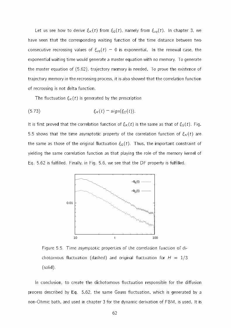
Let us see how to derive �K(t) from �G(t), namely from �eq(t). In chapter 3, we

have seen that the corresponding waiting function of the time distance between two

consecutive recrossing values of �eq(t) = 0 is exponential. In the renewal case, the

exponential waiting time would generate a master equation with no memory. To generate

the master equation of (5.62), trajectory memory is needed. To prove the existence of

trajectory memory in the recrossing process, it is also showed that the correlation function

of recrossing is not delta function.

The uctuation �K(t) is generated by the prescription

(5.73) �K(t) � sign(�G(t)):

It is �rst proved that the correlation function of �K(t) is the same as that of �G(t). Fig.

5.5 shows that the time asymptotic property of the correlation function of �K(t) are

the same as those of the original uctuation �G(t). Thus, the important constraint of

yielding the same correlation function as that playing the role of the memory kernel of

Eq. 5.62 is ful�lled. Finally, in Fig. 5.6, we see that the DF property is ful�lled.

0.01

10 100t

-ΦK(t)

-ΦG(t)

Figure 5.5. Time asymptotic properties of the correlation function of di-

chotomous uctuation (dashed) and original uctuation for H = 1=3

(solid).

In conclusion, to create the dichotomous uctuation responsible for the di�usion

process described by Eq. 5.62, the same Gauss uctuation, which is generated by a

non-Ohmic bath, and used in chapter 3 for the dynamic derivation of FBM, is used. It is

62

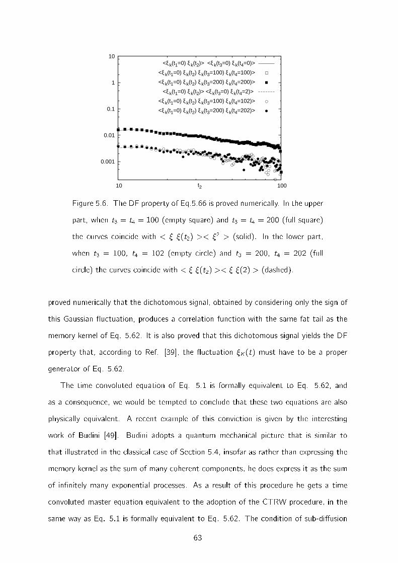
0.001

0.01

0.1

1

10

10 100t2

<ξk(t1=0) ξk(t2)> <ξk(t3=0) ξk(t4=0)>

<ξk(t1=0) ξk(t2) ξk(t3=100) ξk(t4=100)>

<ξk(t1=0) ξk(t2) ξk(t3=200) ξk(t4=200)>

<ξk(t1=0) ξk(t2)> <ξk(t3=0) ξk(t4=2)>

<ξk(t1=0) ξk(t2) ξk(t3=100) ξk(t4=102)>

<ξk(t1=0) ξk(t2) ξk(t3=200) ξk(t4=202)>

Figure 5.6. The DF property of Eq.5.66 is proved numerically. In the upper

part, when t3 = t4 = 100 (empty square) and t3 = t4 = 200 (full square)

the curves coincide with < � �(t2) >< �2 > (solid). In the lower part,

when t3 = 100, t4 = 102 (empty circle) and t3 = 200, t4 = 202 (full

circle) the curves coincide with < � �(t2) >< � �(2) > (dashed).

proved numerically that the dichotomous signal, obtained by considering only the sign of

this Gaussian uctuation, produces a correlation function with the same fat tail as the

memory kernel of Eq. 5.62. It is also proved that this dichotomous signal yields the DF

property that, according to Ref. [39], the uctuation �K(t) must have to be a proper

generator of Eq. 5.62.

The time convoluted equation of Eq. 5.1 is formally equivalent to Eq. 5.62, and

as a consequence, we would be tempted to conclude that these two equations are also

physically equivalent. A recent example of this conviction is given by the interesting

work of Budini [49]. Budini adopts a quantum mechanical picture that is similar to

that illustrated in the classical case of Section 5.4, insofar as rather than expressing the

memory kernel as the sum of many coherent components, he does express it as the sum

of in�nitely many exponential processes. As a result of this procedure he gets a time

convoluted master equation equivalent to the adoption of the CTRW procedure, in the

same way as Eq. 5.1 is formally equivalent to Eq. 5.62. The condition of sub-di�usion

63

makes it legitimate to claim for this equivalence, with the warning though of considering

the results of Section 5.3 proving that within the Liouville perspective the memory kernel

of the time convoluted equation is an equilibrium correlation function, while in the CTRW

perspective is not.

In the case of super-di�usion, it is impossible to derive the time convoluted di�usion

equation of Eq. 5.62 from within the CTRW perspective. This �ts the conclusions of

Balescu [34]. It is interesting to notice that in this case the memory density re ects

correctly the trajectory density. In fact, albeit with the help of numerical rather than

only by means of theoretical arguments, in Section 5.5 it is proved that the dichotomous

uctuation �k , with trajectory memory, generates the di�usion process driven by Eq.

5.62. The search for the dichotomous uctuation responsible for this kind of di�usion

traces back to the work of Ref. [39] and to the earlier work of Ref. [50]. The failure of

these earlier attempts is due to the fact that renewal uctuations, namely memoryless

trajectories, have been searched as generators of this di�usion process. Ref. [51] shows

that the renewal condition violates the DF condition which is essential for the validity

of Eq. 5.62. To solve this long-standing problem, it was necessary to shed light �rst of

all on the confusion, existing in literature, between density and trajectory memory. The

di�usion process described by Eq. 5.62 turned out to be characterized by both trajectory

and density memory.

64

CHAPTER 6

CONCLUSION

In this work, It has been proved that the FBM �ts the constraint of yielding both an

in�nite memory, resulting from the cooperation of the individual bath constituents, and

the renewal aging. To prove that the former property is compatible with the latter it was

necessary to defeat the prejudice that the FBM in�nite memory establishes correlation

among di�erent recrossing of x = 0. The variable x(t) generates non-Poisson renewal

and the highly correlated nature of the variable �(t) is a signature of cooperation. The

important role of cooperation seems to be weakened by the condition H = 0:5, which

generates non-Poisson renewal without involving any cooperation. However, it must be

stress that this is a singularity, and that an even small deviation generates trajectory

memory, as a re ection of cooperation.

Since FBM is a process with in�nitely long range memory dependence, it is not easy

to simulate numerically. The renewal and cooperation model is not successful because of

limited numerical environment but it helps to explain the picture behind the FBM. There

are two successful methods of generating FBM for both sub-di�usion and super-di�usion

case. In the �rst one, using Fourier method, it was possible to generate correlated noise

as much as required but the power law function has to have a cut-o� value. This method

is better used for getting a large enough number of recrossing times. The second one,

the Voss algorithm, has no cut-o� value and it gives better scaling but the trajectory

length is limited.

The process of surface growth is also studied. In that case, particles obey to the

sticking rule and that causes a cooperation among the columns. The study the jumps of

a reference column shows that the process is close to FBM. Also, single column is able

to show the cooperation among the columns.

65

This thesis proves that the generally accepted conviction that FBM is a process with

in�nite memory is incorrect. In fact, the space variable in the asymptotic time regime

yields the FBM scaling in a full agreement with the renewal theory. This thesis establishes

the existence of two forms of memory:

(a) The trajectory memory. The single trajectories have memory of the earlier con-

ditions. An example of this form of memory is the velocity generated by the non-Ohmic

bath. In the non-Ohmic case the time evolution of the variable velocity, described by a

generalized Langevin equation, depends on the past history of the variable itself.

(b) The density memory. In this case the time evolution of a probability distribution

density depends on its past history through a time convoluted structure.

In chapter 5, it has been shown that the trajectory memory does not necessarily yield

density memory. In fact, the di�usion equation generating the FBM scaling has a time

dependent di�usion coe�cient, but does not have a time convoluted structure as seen

in the di�usion equation, Eq. 5.2. FBM is compared with a di�erent kind of di�usion,

CTRW, as seen in Eq. 5.1. The subordination approach to normal di�usion, resting

on trajectory without memory, has, on the contrary, a time convoluted structure. This

means that a non-Poisson renewal process, although corresponding to trajectories with

memory erasing jumps, yields memory at the density level. In the third case, Liouville-

like approach is studied, which shows both trajectory memory and density memory as in

Eqs. 5.69, 5.69 and 5.62. This last approach is used to explain dichotomized fractional

Brownian motion.

66

APPENDIX A

SOLUTION OF THE ORDINARY DIFFUSION EQUATION

67

The di�usion equation can be derived from the continuity equation. It states that a

change in density in any part of the system is due to in ow and out ow of material into

and out of that part of the system. E�ectively, no material is created or destroyed.

(A.1)@@tp(r; t) +r � j = 0;

where j is the ux of the di�using material. The di�usion equation can be obtained easily

from this when combined with the Fick's �rst law, which assumes that the ux of the

di�using material in any part of the system is proportional to the local density gradient.

(A.2) j = �D rp(r; t):

If D is a constant, the equation reduces to the following linear equation:

(A.3)@@tp(r; t) = Dr2p(r; t)

Let us start the solution with the one dimensional equation.

(A.4)@p@t

= D@2p@x2

Take Fourier transform with respect to x using p(k; t) =∫1�1 e�ikxp(x; t)dx . And so

(A.5)∫ 1

�1e�ikx @

2

@x2p(x; t) =∫ 1

�1(�k2)e�ikxp(x; t)dx = �k2p(k; t)

by separation by parts. The equation becomes

(A.6)@@tp(k; t) = �k2Dp(k; t):

This is an �rst order di�erential equation. The solution is simply

(A.7) p(k; t) = C(k)e�Dk2t :

First, the expression of C(k) is required. For t = 0, C(k) = p(k; 0) and

(A.8) p(k; 0) =∫ 1

�1e�ikxp(x; 0)dx:

The initial condition is p(x; 0) = �(x). Since it is a delta function the answer will be the

Green function. So, from the above equation simply, p(k; 0) = 1 = C(k). And so

(A.9) p(k; t) = e�Dk2t :

68

This is the solution of the di�usion equation but it must be converted back to x space.

The inverse Fourier will be

(A.10) p(x; t) =1

2�

∫ 1

�1e ikxp(k; t)dk:

So,

(A.11) p(x; t) =1

2�

∫ 1

�1e ikxe�Dk2tdk =

12�

∫ 1

�1e�Dk2t+ikxdk:

Let's play a little with the exponential part

(A.12)

�Dk2t+ikx = �Dt(k2� ikxDt

) = �Dt[

(k � ix2Dt

)2 +x2

4D2t2

]= �Dt

[(k � ix

2Dt)2

]� x2

4Dt:

and put it into the integral

(A.13) p(x; t) =1

2�e� x2

4Dt

∫ 1

�1e�Dt(k� ix

2Dt )2dk:

Set k � ix2Dt = s and so dk = ds. The integral is

(A.14)∫ 1

�1e�Dts2

ds =√

�Dt

Finally, we get the well-known solution.

(A.15) p(x; t) =1

2�e� x2

4Dt

√�Dt

=1p

4�Dte� x2

4Dt

69

APPENDIX B

SOLUTION OF THE GENERALIZED DIFFUSION EQUATION OF FBM

70

Here will be shown the solution of the generalized di�usion equation,

(B.1)@p@t

= D(∫ t

0��(t)dt 0

)@2p@x2 :

Take Fourier transform with respect to x and the equation becomes

(B.2)@@tp(k; t) = �k2D

(∫ t

0��(t 0)dt 0

)p(k; t):

Similar to App.A, the solution can be obtained as follows:

(B.3)@p(k; t)@t

1p(k; t)

= �k2D(∫ t

0��(t 0)dt 0

)

(B.4) ln p(k; t) = �k2D

(∫ t

0

∫ t 0

0��(t 00)dt 0dt 00

)+ C 0(t)

(B.5) ln p(k; t) = �k2D2< x2(t) > +C 0(t)

(B.6) p(k; t) = C(t) exp(�k2D

2< x2(t) >

):

Using Eqn. D.7, < x2 >= 2 < �2 >∫ t

0 dt0 ∫ t 0

0 ds��(js j) and since � is Gaussian noise

with zero average and unit mean < �2 >= 1, Again, C(k) = 1 for x(t = 0) = 0 and

p(x; 0) = �(x) as App. A, and C(t) = exp(C 0(t)). And so

(B.7) p(k; t) = e�D2 k

2<x2(t)>:

The inverse Fourier will be as follows:

(B.8) p(x; t) =1

2�

∫ 1

�1e ikxe�D

2 k2<x2(t)>dk

(B.9) p(x; t) =1

2�

∫ 1

�1e�

D2 <x

2(t)>[k� ix(t)

D<x2(t)>

]2� x2(t)2D<x2(t)>dk

(B.10) p(x; t) =1

2�e�

x2(t)2D<x2(t)>

∫ 1

�1e�

D2 <x

2(t)>[k� ix(t)

D<x2(t)>

]2

dk

(B.11) p(x; t) =1

2�e�

x2(t)2D<x2(t)>

√�

D2 < x2(t) >

71

(B.12) p(x; t) =1√

2�D < x2(t) >e�

x2(t)2D<x2(t)>

72

APPENDIX C

ASYMPTOTIC SOLUTION OF THE GENERALIZED DIFFUSION EQUATION OF

FBM

73

It will be shown that, when t ! 1, Eqn. 2.3 is solution of Eqn. 2.4. Di�usion

equation for FBM is

(C.1) pt = D C(t) pxx

where C(t) =∫ t

0 dt0�(t 0), p = p(x; t), pt = @p

@t and pxx = @2p@x2 .

Using

p =t�Hp4�D

exp(� x2

4Dt�2H

):(C.2)

pt = � 1p4�D

exp(� x2

4Dt�2H

){Ht�(H+1) +

x2

4Dt�(3H+1)

}(C.3)

px =t�H4�D

exp(� x2

4Dt�2H

)(�2xt�2H

4D

)(C.4)

pxx = � 1p4�D

exp(� x2

4Dt�2H

){1

2Dt�3H +

x2

4D2 t�5H

}(C.5)

we get

C(t) =pt

D pxx=Ht�(H+1) + x2

4D t�(3H+1)

12t�3H + x2

4D t�5H= t2H�1Ht

2H + x2

4D12t2H + x2

4D

:(C.6)

For H = 1=2, C(t)=1, and

limt!1

Ht2H + x2

4D12t2H + x2

4D

= 2H for H < 1=2(C.7)

limt!1

Ht2H + x2

4D12t2H + x2

4D

= limt!1

H + x2

4D t�2H

12 + x2

4D t�2H= 2H for H > 1=2:(C.8)

So, from Eqn. 2.14 for D = h�2i and H = H,

limt!1

ddtC(t) = 2H(2H � 1)t2H�2 =

h�2iD

��(t) = ��(t):(C.9)

74

APPENDIX D

RELATION BETWEEN THE VARIANCE AND THE STATIONARY CORRELATION

FUNCTION OF FBM

75

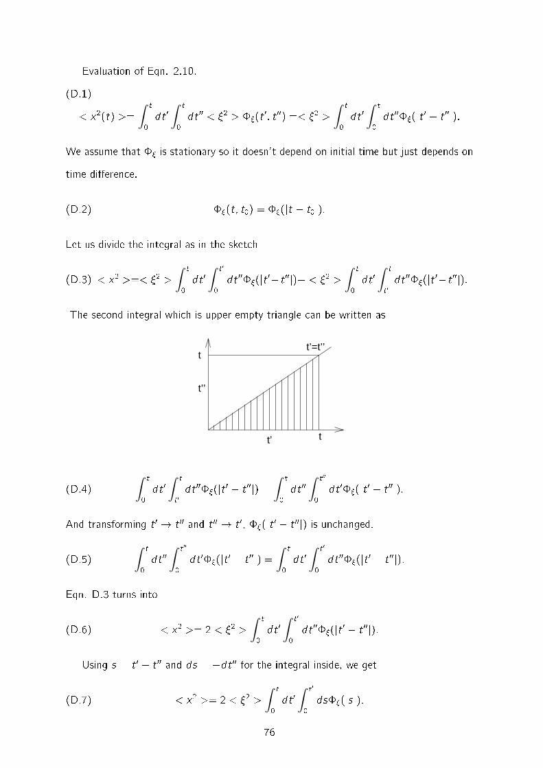
Evaluation of Eqn. 2.10.

(D.1)

< x2(t) >=∫ t

0dt 0

∫ t

0dt 00 < �2 > ��(t 0; t 00) =< �2 >

∫ t

0dt 0

∫ t

0dt 00��(jt 0 � t 00j):

We assume that �� is stationary so it doesn't depend on initial time but just depends on

time di�erence.

(D.2) ��(t; t0) = ��(jt � t0j):

Let us divide the integral as in the sketch

(D.3) < x2 >=< �2 >∫ t

0dt 0

∫ t 0

0dt 00��(jt 0�t 00j)+ < �2 >

∫ t

0dt 0

∫ t

t 0dt 00��(jt 0�t 00j):

The second integral which is upper empty triangle can be written as

t’

t’’

t

t

t’=t’’

(D.4)∫ t

0dt 0

∫ t

t 0dt 00��(jt 0 � t 00j) =

∫ t

0dt 00

∫ t 00

0dt 0��(jt 0 � t 00j):

And transforming t 0 ! t 00 and t 00 ! t 0, ��(jt 0 � t 00j) is unchanged.

(D.5)∫ t

0dt 00

∫ t 00

0dt 0��(jt 0 � t 00j) =

∫ t

0dt 0

∫ t 0

0dt 00��(jt 0 � t 00j):

Eqn. D.3 turns into

(D.6) < x2 >= 2 < �2 >∫ t

0dt 0

∫ t 0

0dt 00��(jt 0 � t 00j):

Using s = t 0 � t 00 and ds = �dt 00 for the integral inside, we get

(D.7) < x2 >= 2 < �2 >∫ t

0dt 0

∫ t 0

0ds��(jsj):

76

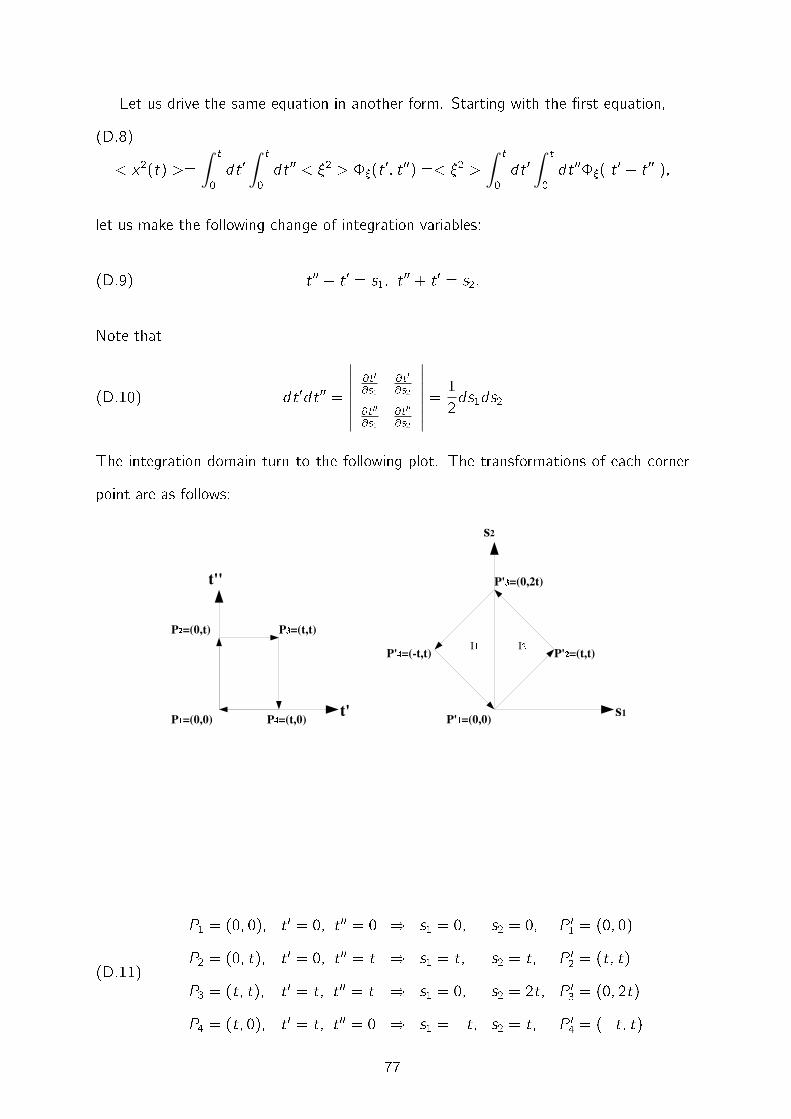
Let us drive the same equation in another form. Starting with the �rst equation,

(D.8)

< x2(t) >=∫ t

0dt 0

∫ t

0dt 00 < �2 > ��(t 0; t 00) =< �2 >

∫ t

0dt 0

∫ t

0dt 00��(jt 0 � t 00j);

let us make the following change of integration variables:

(D.9) t 00 � t 0 = s1; t 00 + t 0 = s2:

Note that

(D.10) dt 0dt 00 =

∣∣∣∣∣∣∣

@t 0@s1

@t 0@s2

@t 00@s1

@t 00@s2

∣∣∣∣∣∣∣=

12ds1ds2

The integration domain turn to the following plot. The transformations of each corner

point are as follows:

(D.11)

P1 = (0; 0); t 0 = 0; t 00 = 0 ) s1 = 0; s2 = 0; P 01 = (0; 0)

P2 = (0; t); t 0 = 0; t 00 = t ) s1 = t; s2 = t; P 02 = (t; t)

P3 = (t; t); t 0 = t; t 00 = t ) s1 = 0; s2 = 2t; P 03 = (0; 2t)

P4 = (t; 0); t 0 = t; t 00 = 0 ) s1 = �t; s2 = t; P 04 = (�t; t)77

The integral is divided into two parts.

(D.12)I1 =

∫ 0�t ds1

∫ s1+2t�s1

�(s1) =∫ 0�t ds1(2t + 2s1)�(s1)

=∫ t

0 ds1(2t � 2s1)�(s1)

with s1 ! �s1 and using �(�s1) = �(s1).

(D.13) I2 =∫ t

0ds1

∫ �s1+2t

s1

�(s1) =∫ t

0ds1(2t � 2s1)�(s1) = I1:

Finally, the result is

(D.14)< x2(t) > = < �2 > 1

2 [I1 + I2] =< �2 > 12 2

∫ t0 ds1(2t � 2s1)�(s1)

= 2 < �2 >∫ t

0 ds1(t � s1)�(s1)

78

APPENDIX E

RELATION BETWEEN THE VARIANCE AND THE SCALING OF FBM

79

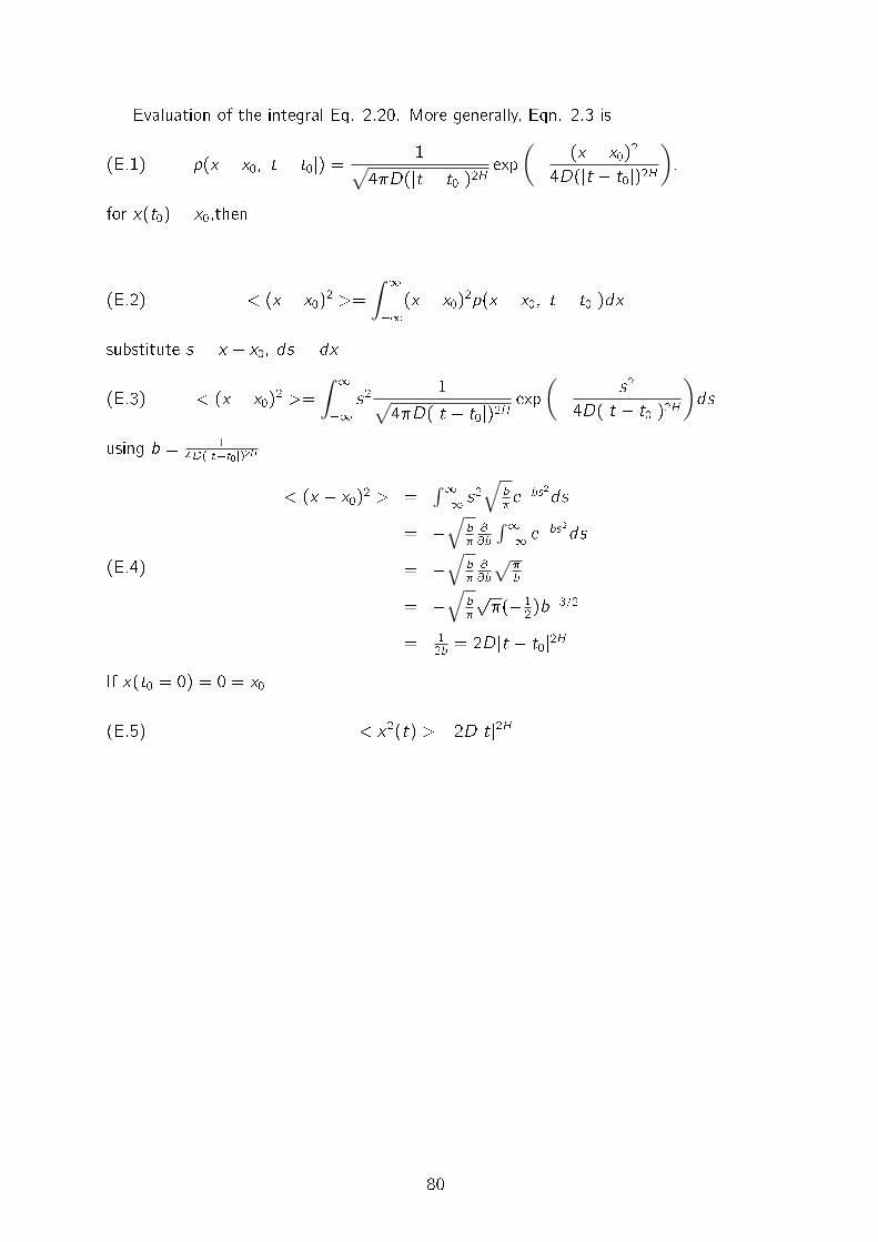
Evaluation of the integral Eq. 2.20. More generally, Eqn. 2.3 is

(E.1) p(x � x0; jt � t0j) =1√

4�D(jt � t0j)2Hexp

(� (x � x0)2

4D(jt � t0j)2H

):

for x(t0) = x0,then

(E.2) < (x � x0)2 >=∫ 1

�1(x � x0)2p(x � x0; jt � t0j)dx

substitute s = x � x0, ds = dx

(E.3) < (x � x0)2 >=∫ 1

�1s2 1√

4�D(jt � t0j)2Hexp

(� s2

4D(jt � t0j)2H

)ds

using b = 14D(jt�t0j)2H

(E.4)

< (x � x0)2 > =∫1�1 s2

√b�e�bs2ds

= �√

b�@@b

∫1�1 e�bs

2ds

= �√

b�@@b

√�b

= �√

b�

p�(�1

2 )b�3=2

= 12b = 2Djt � t0j2H

If x(t0 = 0) = 0 = x0

(E.5) < x2(t) >= 2Djtj2H

80

APPENDIX F

DIFFUSION ENTROPY

81

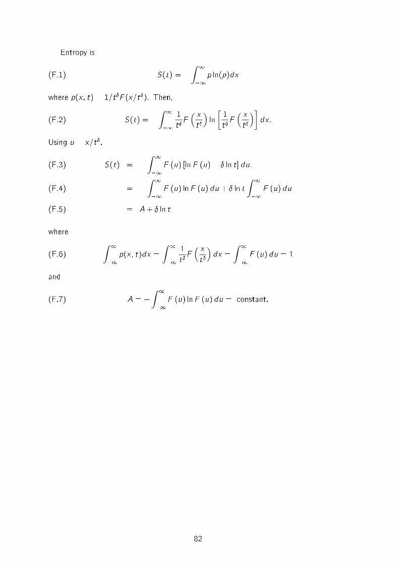
Entropy is

(F.1) S(t) = �∫ 1

�1p ln(p)dx

where p(x; t) = 1=t�F (x=t�). Then,

(F.2) S(t) = �∫ 1

�11t�F

( xt�

)ln

[1t�F

( xt�

)]dx:

Using u = x=t�,

S(t) = �∫ 1

�1F (u) [lnF (u)� � ln t] du:(F.3)

= �∫ 1

�1F (u) lnF (u) du + � ln t

∫ 1

�1F (u) du(F.4)

= A+ � ln t(F.5)

where

(F.6)∫ 1

�1p(x; t)dx =

∫ 1

�11t�F

( xt�

)dx =

∫ 1

�1F (u) du = 1

and

(F.7) A = �∫ 1

�1F (u) lnF (u) du = constant.

82

APPENDIX G

ON THE PROBABILITY OF THE RECROSSING TIMES

83

It is important to calculate the function n(t), the probability density of occurrence

of the nth recrossing at time t. The recrossing times are statistically independent so the

probability of having 2 recrossing times together is 1(�1) 1(�2) = (�1) (�2), where

the probability of having 1 recrossing, 1(�), is just (�).

To get he probability 2(t), all possible intermediate time between 0 and t must be

considered. Let us keep �1 + �2 = t, we have

(G.1) 2(t) =∫ t

0d� 1(�) 1(t � �):

Similarly, the function n(t) is related to n�1(t) by

(G.2) n(t) =∫ t

0d� n�1(�) 1(t � �);

Using the convolution theorem of Laplace transform, we get

(G.3) n(u) = n�1(u) 1(u):

On the other hand,

(G.4) n�1(u) = n�2(u)(�) 1(u):

That gives

(G.5) n(u) = n�2(u)( 1)2(u):

Bay iterating this procedure, we get

(G.6)

n(u) = n�3(u)( 1)3(u):

: : :

n(u) = 0(u)( 1)n(u):

Note that 0(t) = �(t). That means the probability of having the 0th recrossing at t > 0

is zero since it is certainly at t = 0 that is x(t0 = 0) = 0. An so 0(t) = L[�(t)] = 1:

Finally that gives the important result

(G.7) n(u) = ( (u))n:

84

APPENDIX H

LAPLACE TRANSFORM OF THE POWER LAW FUNCTION WITH SLOPE

1 < � < 2

85

Let us consider

(H.1) �(t) =(�� 1)T ��1

(t + T )�:

From the work of Mauro Bologna [8]

(H.2) (u) =(�� 1)�(1� �)

(uT )1��[euT � EuT��1

];

where

(H.3) EuT��1(T ) =1∑n=0

(uT )n+1���(n + 2� �)

:

Using Eqn. H.1, the Taylor series expansion of Eqn. H.3 and �(2��) = (1��)�(1��),

we get:

(H.4)

�(u) = �(�� 1)�(1� �)(uT )1��

{(uT )1���(2� �)

+(uT )2���(3� �)

+(uT )3���(4� �)

+ � � �

�1� uT � 12

(uT )2 � 16

(uT )3 + � � �}

={

1 +�(2� �)(uT )

�(3� �)+

�(2� �)(uT )2

�(4� �)+ � � �

��(2� �)[

(uT )��1 + (uT )� +12

(uT )�+1 +16

(uT )�+2 + � � �]}

:

In the case of range 1 < � < 2, the slowest decay is given by (uT )��1. Thus:

(H.5) limu!0

(u) = 1� �(2� �)T ��1u��1

86

APPENDIX I

CORRELATION FUNCTION OF THE DIFFUSION VARIABLE OF FBM

87

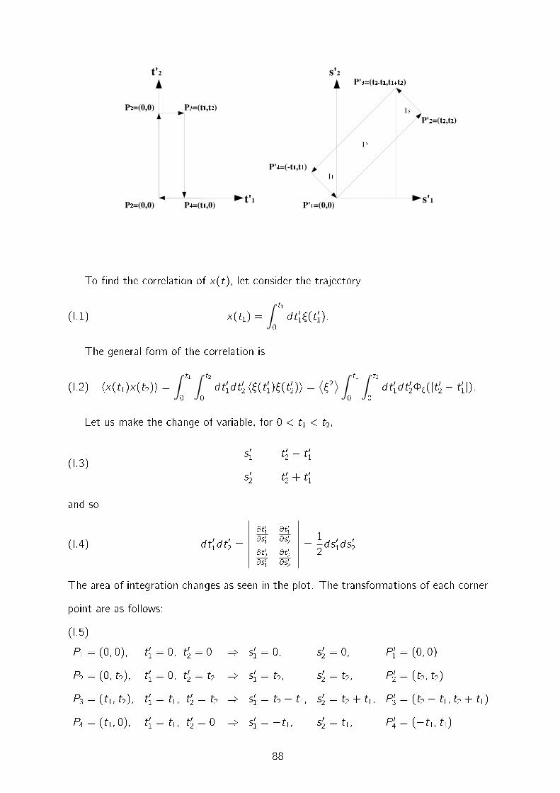
To �nd the correlation of x(t), let consider the trajectory

(I.1) x(t1) =∫ t1

0dt 01�(t 01):

The general form of the correlation is

(I.2) hx(t1)x(t2)i =∫ t1

0

∫ t2

0dt 01dt 02 h�(t 01)�(t 02)i =

⟨�2⟩

∫ t1

0

∫ t2

0dt 01dt 02��(jt 02 � t 01j):

Let us make the change of variable, for 0 < t1 < t2,

(I.3)s 01 = t 02 � t 01s 02 = t 02 + t 01

and so

(I.4) dt 01dt 02 =

∣∣∣∣∣∣∣

@t 01@s 01

@t 01@s 02

@t 02@s 01

@t 02@s 02

∣∣∣∣∣∣∣=

12ds 01ds 02

The area of integration changes as seen in the plot. The transformations of each corner

point are as follows:

(I.5)

P1 = (0; 0); t 01 = 0; t 02 = 0 ) s 01 = 0; s 02 = 0; P 01 = (0; 0)

P2 = (0; t2); t 01 = 0; t 02 = t2 ) s 01 = t2; s 02 = t2; P 02 = (t2; t2)

P3 = (t1; t2); t 01 = t1; t 02 = t2 ) s 01 = t2 � t1; s 02 = t2 + t1; P 03 = (t2 � t1; t2 + t1)

P4 = (t1; 0); t 01 = t1; t 02 = 0 ) s 01 = �t1; s 02 = t1; P 04 = (�t1; t1)

88

After this, the integral is divided into there parts.

(I.6)

I1 =∫ 0�t1 ds

01

∫ (s 01+t1)+t1�(s 01+t1)+t1

ds 02��(s 01)

=∫ 0�t1 ds

012(s 01 + t1)��(s 01)

set s 01 ! �s1 and using �(�s1) = �(s1)

= �2∫ 0t1ds1(t1 � s1)��(s1) = 2

∫ t10 ds1(t1 � s1)��(s1)

(I.7) I2 =∫ t2�t1

0 ds 01∫ s 01+2t1s 01

ds 02��(s 01) = 2t1∫ t2�t1

0 ds 01��(s 01)

(I.8)

I3 =∫ t2t2�t1 ds

01

∫ �(s 01�(t2�t1))+t1+t2s 01

ds 02��(s 01)

= 2∫ t2t2�t1 ds

01(t2 � s 01)��(s 01)

= 2∫ t2

0 ds 01(t2 � s 01)��(s 01)� 2∫ t2�t1

0 ds 01(t2 � s 01)��(s 01)

Let us add the integrals to get the correlation.

(I.9)

hx(t1)x(t2)i = 12 h�2i [I1 + I2 + I3]

= h�2i[∫ t1

0 ds 01(t1 � s 01)��(s 01) +∫ t2�t1

0 ds 01t1��(s 01)

+∫ t2

0 ds 01(t2 � s 01)��(s 01)� ∫ t2�t10 ds 01(t2 � s 01)��(s 01)

]

= h�2i[∫ t1

0 ds 01(t1 � s 01)��(s 01) +∫ t2

0 ds 01(t2 � s 01)��(s 01)� ∫ t2�t10 ds 01(t2 � t1 � s 01)��(s 01)

]

Repeating the same calculation for 0 < t2 < t1, the same result will be obtained as t1

and t2 are interchanged because of the symmetry in Eqn. I.2. As a result, the correlation

is

(I.10)hx(t1)x(t2)i = h�2i

[∫ t10 ds 01(t1 � s 01)��(s 01) +

∫ t20 ds 01(t2 � s 01)��(s 01)

� ∫ jt2�t1j0 ds 01(jt2 � t1j � s 01)��(s 01)

]

Using Eqn.D.14, it can be written as

(I.11) hx(t1)x(t2)i =12

[< x2(jt1j) > + < x2(jt2j) > � < x2(jt1 � t2j) >]

and using Eqn. E.5, it becomes

(I.12) hx(t1)x(t2)i =< �2 >[jt1j2H + jt2j2H � jt1 � t2j2H]

;

which is the popular result found years ago by Mandelbrot and Van Ness [1].

89

If it is normalized to initial time, for t1 = t and t2 = t0, the result is

(I.13)

<x(t)x(t0)><x2(t0)> = (jtj2H + jt0j2H � jt � t0j2H)=2jt0j2H

= 12

(( jtjjt0j)

2H + 1� ( jt�to jjt0j )2H)

= 12

(∣∣∣ tt0∣∣∣

2H+ 1�

∣∣∣ tt0 � 1∣∣∣

2H)

If t0 = �t and t = t in Eqn. I.13, and < x2(�t) >=< x2(jtj) >, from Eqn. E.5

(I.14)< x(t)x(�t) >< x2(t) >

=12

(2� 22H) = 1� 22H�1:

90

APPENDIX J

RELATION BETWEEN THE MEMORY KERNEL AND THE POWER LAW

DISTRIBUTION OF CTRW

91

Let us consider the following picture

(J.1) p(t) =1∑n=0

∫ t

0 n(�)(t � �)Mnp(0)d�:

The time convoluted structure of Eq. J.1 suggests the use of the Laplace transform

method. Let us use the de�nition:

(J.2) �(u) =∫ 1

0e�ut�(t`)dt`:

Using App. G, we use the following result:

(J.3) n(u) = ( (u))n:

Given the important the fact that the last event occurred at t` < t, we have to make

it sure that in the residual time of length t � t` no event does occur. This is the reason

why in Eq. J.1 we have to use the function (t), whose meaning is de�ned by

(J.4) (t) =∫ 1

t 1(t`)dt`:

Note that

(J.5)∫ 1

0 1(t`)dt` = 1:

This is so because the distribution density 1(t) is a probability that one event occurs

somewhere between t = 0 and t = 1 must be 1. We do not know when the event

occurs. We know that it does somewhere between t = 0 and t =1. Thus

(J.6) (t) =∫ 1

t 1(t`)dt` =

∫ 1

0 1(t`)dt �

∫ t

0 1(t`)dt` = 1�

∫ t

0 1(t`)dt`

Using L[∫ t

0 f (t 0)dt 0] = f (t)=u and L[1] = 1=u for u > 0, we �nd

(J.7) (t) =1� (u)

u:

In conclusion, both n(t) and (t) can be expressed in terms of 1(t). This makes

1(t) so important that it is required to adopt a special notation for it, namely,

(J.8) (t) = 1(t):

92

Let us evaluate the Laplace transform of Eq. J.1. We get:

(J.9) p(t) =1∑n=0

n(u)(u)Mnp(0):

Using Eq.J.3 and J.7, and assumption 0(t)�(t), we get:

(J.10)p(t) =

∑1n=0( (u))n 1

u (1� (u))Mnp(0)

=∑1

n=0( (u)Mn)n 1u (1� (u))p(0):

On the other hand,

(J.11)1∑n=0

( (u)Mn)n =1

1� (u)M:

Thus Eq. J.9 becomes:

(J.12) p(t) =1u

1� (u)1� (u)M

p(0):

This is a way to connect the distribution at time t to the initial state p(0). To

establish the equivalence of Eq J.1 to

(J.13)@@t

p(t) = �∫ t

0d��(�)Kp(t � �) = �

∫ t

0d��(t � �)Kp(�);

let us evaluate Laplace transform of Eq. J.13. We get:

(J.14) up(u)� p(0) = ��(u)K � p(u);

yielding:

(J.15) p(u) =1

u + �(u)Kp(0):

By comparing Eq. J.12 and Eq. J.15, we get:

(J.16) u + �(u)K =u(1� (u)M)

(1� (u)):

Thus we get:

(J.17) �(u)K =u (u)(1�M)

(1� (u)):

It is convenient to get

(J.18) K = M� 1

93

and from Eq. J.17,

(J.19) �(u) =u (u)

(1� (u)):

94

APPENDIX K

DERIVATION OF THE AUXILARY FUNCTION

95

Let us �nd the equation of motion of

(K.1)dydt

= �y z ;

where z > 1 and 0 < � � 1. For z = 1, it is ordinary random walk and the solution is

easy. Sabstitute u = y 1�z and so du=dt = dy=dt(1� z)y�z .

(K.2)dudt

y z

1� z = �y z :

By eliminating y z and integrating this equation we get:

(K.3) u = (1� z)�t + C = y 1�z :

For t = 0, y = y0 so it gives C = y 1�z0 . And �nal form becomes:

(K.4) y =[(1� z)�t + y 1�z

0

] 11�z

This is the position variable. To �nd the velocity, which is the stochastic noise, the

derivative of Eq, K.4 is needed. That gives:

(K.5)dydt

= �A =�y z0[

1� (z � 1)�y z�10 t

] z1�z:

Sabstituting

(K.6) � =z

z � 1;

we get:

(K.7) �A(t) =�y

���1

0[1� y 1

��10

���1t

]�

and also for Eq. K.4

(K.8) y(t) =y0[

1� y 1��1

0���1t

]��1 :

The initial position y0 is chosen randomly in [0 : 1] and when y(t = �) = 1, the motion

ends and restarts with a random initial position y0. Now let us �nd the distribution of

96

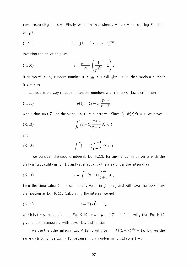
these recrossing times � . Firstly, we know that when y = 1, t = � , so using Eq. K.4,

we get:

(K.9) 1 =[(1� z)�� + y 1�z

0

] 11�z :

Inverting the equation gives:

(K.10) � =�� 1�

1

y1��1

0

� 1

:

It shows that any random number 0 < y0 < 1 will give us another random number

0 < � <1.

Let us see the way to get the random numbers with the power law distribution

(K.11) (t) = (s � 1)T s�1

t + T;

where time unit T and the slope s > 1 are constants. Since∫1

0 (t)dt = 1, we have:

(K.12)∫ r

0(s � 1)

T s�1

t + Tdt < 1

and

(K.13)∫ 1

r(s � 1)

T s�1

t + Tdt < 1

If we consider the second integral, Eq, K.13, for any random number x with the

uniform probability in [0 : 1], and set it equal to the area under the integral as

(K.14) x =∫ 1

r(s � 1)

T s�1

t + Tdt;

then the time value t = r can be any value in [0 : 1] and will have the power law

distribution as Eq. K.11. Calculating the integral we get:

(K.15) r = T (x1

1�s � 1);

which is the same equation as Eq. K.10 for s = � and T = ��1� , showing that Eq. K.10

give random numbers � with power law distribution.

If we use the other integral Eq. K.12, it will give r = T ((1� x)1

1�s � 1). It gives the

same distribution as Eq. K.15, because if x is random in [0 : 1] so is 1� x .

97

APPENDIX L

RELATION BETWEEN THE VARIANCE AND THE MEMORY KERNEL OF CTRW

98

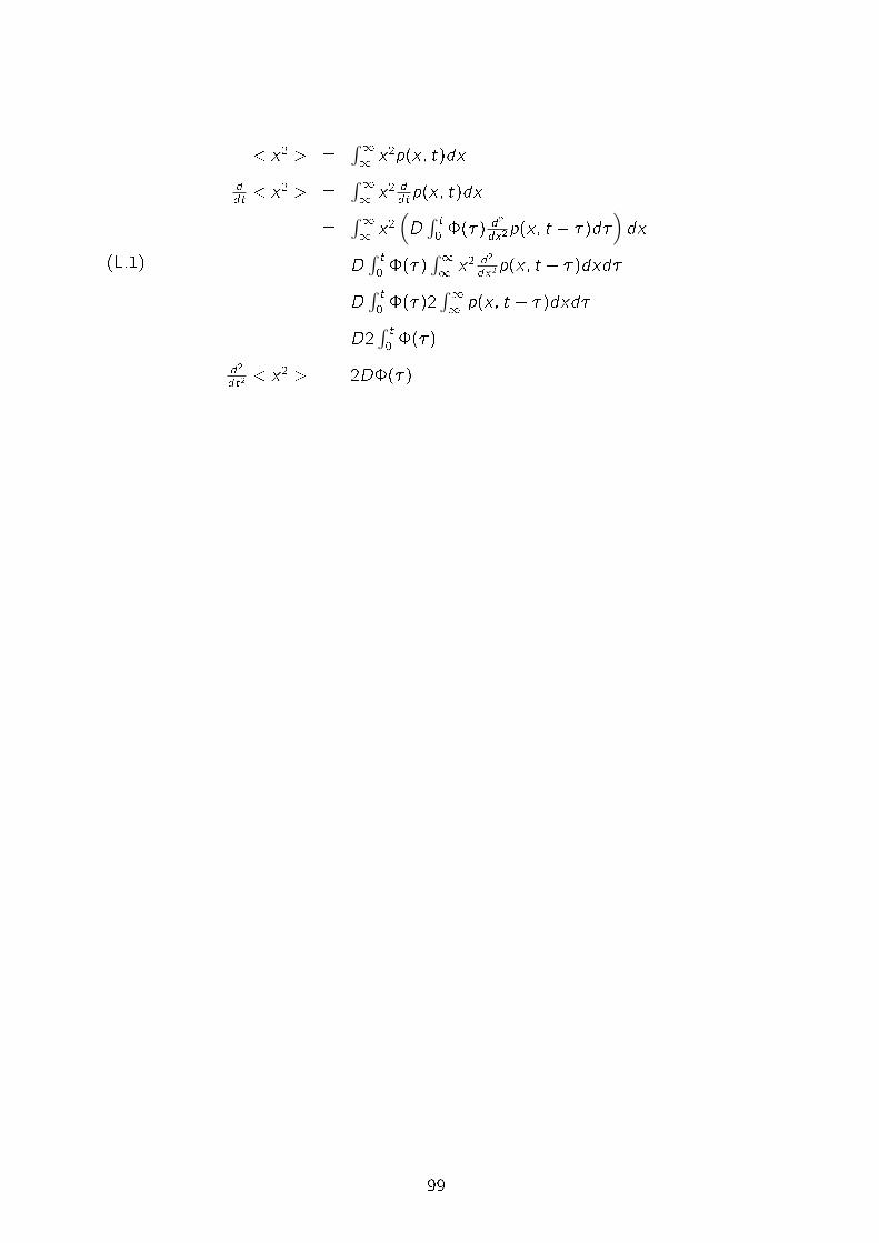
(L.1)

< x2 > =∫11 x2p(x; t)dx

ddt < x2 > =

∫11 x2 d

dtp(x; t)dx

=∫11 x2

(D

∫ t0 �(�) d2

dx2p(x; t � �)d�)dx

= D∫ t

0 �(�)∫11 x2 d2

dx2p(x; t � �)dxd�

= D∫ t

0 �(�)2∫11 p(x; t � �)dxd�

= D2∫ t

0 �(�)

d2

dt2 < x2 > = 2D�(�)

99

APPENDIX M

THE FORM OF MEMORY KERNEL OF CTRW

100

(M.1)

D�(t) = < �2A(t) > +

∫ t0 dt` ddt < �A(t)�A(t`) >

= C(t+T )(2��) +

∫ t0 dt` ddt

[C

(t+T )2��F (t � t`)]

= C(t+T )(2��) +

∫ t0 dt`

[(��2)C

(t+T )3��F (t � t`) + C(t+T )2��

dFdt

]

= C(t+T )(2��) +

∫ t0 dt` (��2)C

(t+T )3��F (t � t`) +∫ t

0 dt` C(t+T )2��

dFdt

= C(t+T )(2��) +

∫ t0 du

(��2)C(t+T )3��F (u) +

∫ t0 du

C(t+T )2��

dFdt

= C(t+T )(2��) � (2��)C

(t+T )3��∫ t

0 F (u)du + C(t+T )2�� [F (t)� F (0)]

= � (2��)C(t+T )3�� F (0) + C

(t+T )2��F (t)

where we used u = t � t`, F (0) = 1 and F (0) =∫ t

0 F (u)du.

101

REFERENCES

[1] Mondelbrot B. B., Van Ness J., The Fractinal Brownian motions, fractional noises, and applications,

SIAM Rev., 10, 422 (1968).

[2] R. Failla, M. Ignaccolo, P. Grigolini and A. Schwettmann, Phys. Rev E 70 R, 010101 (2004).

[3] Weiss U., The Fractal Geometry of Nature, World Scienti�c, Singapore (1999).

[4] Pottier N., Physics A 317, 371 (2003).

[5] Mondelbrot B. B., Quantum Dissipative Systems, Freeman, New York (1977).

[6] Feder J., The Fractals, Plenum Press, New York (1988).

[7] F. M. Izrailev, A.A. Krokhin, and S. E. Ulloa,Phys. Rev. B 63, 041102(R) (2001).

[8] Bologna M., Chem. Phys. B, 284 (2002).

[9] Godreche G., Luck J. M., J. Stat. Phys., 104, 489 (2001).

[10] Aquino G., Bologna M., Grigolini P., West B. J., Phys. Rev. E, 70, 036105 (2004.

[11] Feder J., Fractals, Plenum Press, New York, London (1988).

[12] M. Kardar, G. Parisi, and Y.-C. Zhang, Phys. Rev. Lett. 56 889 (1986).

[13] H.E. Stanley and A. L. Barabasi, Fractal Concepts in Surface Growth, Cambridge University Press,

Cambridge (1995).

[14] S. N. Majumdar and D. Das, Phys. Rev. E 71, 036129 (2005).

[15] M. Constantin, C. Dasgupta, P. P. Chatraphorn, S. N. Majumdar, and S. Das Sarma, Phys. Rev. E

69, 061608 (2004).

[16] J. -F. Muzy, E. Bacry, Phys. Rev. E 66, 056121 (2002).

[17] R. Zwanzig, J. Chem. Phys. 33, 1338 (1960).

[18] R. Zwanzig, Nonequilibrium Statistical Mechanics, Oxford University Press, Oxford (2001).

[19] H. Mori, Prog. Theor. Phys. 33, 423 (1965); 34, 399 (1965).

[20] Memory Function Approaches to Stochastic Problems in Condensed Matter, eds. M. W. Evans, P.

Grigolini, G. Pastori Parravicini, Advances in Chemical Physics, Volume 62, J. Wiley New York (1985).

[21] U. Balucani, M. H. Lee and V. Tognetti, Phys. Rep. 373, 409 (2003).

[22] R. Zwanzig, Physica 30, 1109 (1964).

[23] I. Prigogine and P. R�esibois, Physica 27, 629 (1961).

[24] R. Balescu, Equilibrium and Nonequilibrium Statistical Mechanics, Wiley-Interscience, New York

(1975).

102

[25] B.B. Mandelbrot, The Fractal Geometry of Nature, Freeman, New York (1982).

[26] S. V. Muniandy and S.C. Lim, Phys. Rev. E 66, 021114 (2002).

[27] E.W. Montroll and G. H. Weiss, J. Math. Phys. 6, 167 (1975).

[28] V. M. Kenkre, E.W. Montroll, and M. F. Shlesinger, J. Stat. Phys. 9, 45 (1973).

[29] M. Annunziato, P. Grigolini and J. Riccardi, Phys. Rev. E 61, 4801 (2000).

[30] M. O. C�aceres, Phys. Rev. E 67, 016102 (2003).

[31] P. Grigolini, Phys. Lett. A 119, 157 (1986).

[32] V.M. Kenkre, Granular Matter 3, 23 (2001).

[33] I. M. Sokolov, J. Klafter, Chaos 15, 026103 (2005).

[34] R. Balescu, Aspects of Anomalous Transport in Plasmas, Francis & Taylor, London (2005).

[35] V. M. Kenkre and R.S. Knox, Phys. Rev. B 9, 5279 (1974).

[36] R. Kubo, Adv. Chem. Phys. 16, 101 (1969).

[37] R. Kubo, J. Phys. Soc. (Japan) 26 Suppl, 1 (1969).

[38] P. Grigolini, Chem. Phys. 38, 389 (1979).

[39] M. Bologna, P. Grigolini and B. J. West, Chem. Phys. 284, 115 (2002).

[40] P. Allegrini, P. Grigolini, L. Palatella, and B. J. West Phys. Rev. E 70, 046118 (2004).

[41] P. Allegrini, G. Aquino, P. Grigolini, L. Palatella, and A. Rosa, Phys. Rev. E 68, 056123 (2003).

[42] W. Feller, An Introduction to Probability and Its Applications, vol. 2, Wiley, New York (1971).

[43] M. Ignaccolo, P. Grigolini, and A. Rosa, Phys. Rev. E 64, 026210 (2001).

[44] D. Cohen, Phys. Rev. E 55, 1422 (1997).

[45] N. Pottier, Physica A 317, 371 (2003).

[46] U. Weiss, Quantum Dissipative Systems, 2nd edition, World Scienti�c, Singapore (1999).

[47] F. Mainardi, Chaos, Solitons and Fractals, 7, 1461 (1996).

[48] F. Mainardi, in Fractals and Fractional Calculus in Continuum Mechanics, Springer Verlag, Wien and

New York (1997) A. Carpinteri and F. Mainardi eds., downladable from http://www.fracalmo.org.

[49] A. A. Budini, Phys. Rev. E 72, 056106 (2005).

[50] P. Allegrini, P. Grigolini, B.J. West, Phys. Rev. E 54, 4760 (1996).

[51] P. Allegrini, G. Aquino, P. Grigolini, L. Palatella, A. Rosa, and B. J. West, Phys. Rev. E, 70, 046118

(2004).

103