Time reversal for drifted fractional Brownian motion with ...

$: Time reversal for drifted fractional Brownian motion with ...$
HAL Id: hal-00485652https://hal.archives-ouvertes.fr/hal-00485652

Submitted on 21 May 2010

HAL is a multi-disciplinary open accessarchive for the deposit and dissemination of sci-entific research documents, whether they are pub-lished or not. The documents may come fromteaching and research institutions in France orabroad, or from public or private research centers.

L’archive ouverte pluridisciplinaire HAL, estdestinée au dépôt et à la diffusion de documentsscientifiques de niveau recherche, publiés ou non,émanant des établissements d’enseignement et derecherche français ou étrangers, des laboratoirespublics ou privés.

Time reversal for drifted fractional Brownian motionwith Hurst index H>1/2

Sébastien Darses, Bruno Saussereau

To cite this version:Sébastien Darses, Bruno Saussereau. Time reversal for drifted fractional Brownian motion with Hurstindex H>1/2. Electronic Journal of Probability, Institute of Mathematical Statistics (IMS), 2007, 12,pp.1181-1211. hal-00485652

https://hal.archives-ouvertes.fr/hal-00485652

https://hal.archives-ouvertes.fr

E l e c t r o n ic

Jo

ur n a l

of

Pr

o b a b i l i t y

Vol. 12 (2007), Paper no. 43, pages 1181–1211.

Journal URLhttp://www.math.washington.edu/~ejpecp/

Time reversal for drifted fractional Brownian motion

with Hurst index H > 1/2

Sebastien Darses

Universite Paris VI, LPMA.

4, Place Jussieu, 75252 Paris Cedex 05, France.

[email protected]

Bruno Saussereau

University of Franche-Comte.

UFR Sciences et Techniques. UMR 6623.

16 route de Gray, 25030 Besancon, France.

[email protected]

Abstract

Let X be a drifted fractional Brownian motion with Hurst index H > 1/2. We prove thatthere exists a fractional backward representation of X , i.e. the time reversed process isa drifted fractional Brownian motion, which continuously extends the one obtained in thetheory of time reversal of Brownian diffusions when H = 1/2. We then apply our result tostochastic differential equations driven by a fractional Brownian motion.

Key words: Fractional Brownian motion. Time reversal. Malliavin Calculus.

AMS 2000 Subject Classification: Primary 60G18; 60H07; 60H10; 60J60.

Submitted to EJP on October 27, 2006, final version accepted August 16, 2007.

1181

http://www.math.washington.edu/~ejpecp/

1 Introduction

Time reversal for diffusion processes driven by a Brownian motion (Bm in short) has alreadybeen studied by several authors in the Markovian case (9; 17; 10) and by Follmer (7) in theMarkovian and non Markovian case. The question can be summed up as to know whether thetime reversed process is again a diffusion and how to compute its reversed drift and its reverseddiffusion coefficient. Different approaches have been proposed. Haussmann and Pardoux (9)tackle this problem by means of weak solutions of backward and forward Kolmogorov equations;Pardoux (17) bases its approach on the enlargement of a filtration. In both cases, the reverseddrift, the reversed diffusion coefficient and the Brownian motion driving the reversed diffusion areexplicitely identified. Millet, Nualart and Sanz (10) use the integration by parts from MalliavinCalculus and obtain under mild assumptions the expressions of the reversed drift and diffusioncoefficient.

These approaches find their roots in Follmer’s work (7) for a class of drifted Brownian motions.He gives, under a finite entropy condition, a formula for the reversed drift of a non Markoviandiffusion with a constant diffusion coefficient. He deeply uses the relation between drifts andthe forward and backward derivatives introduced by Nelson (12) in his dynamical theory ofBrownian diffusions. From a dynamical point of view, Nelson’s operators are fundamental toolsas regards Brownian diffusions. Based on these operators, it is possible to define an operatorwhich extends classical differentiation from smooth deterministic functions to classical diffusionprocesses and which allows to give stochastic analogue to standard differential operators (see(3)). Unfortunately these operators fail to exist for a simple fractional Brownian motion (fBmin short) when H 6= 1/2 (cf Proposition 10 of this paper).

The question one may then address is to know if we can obtain a drifted fBm for the time reversedprocess of a drifted fBm, which extends the one obtained in the Brownian case. Despite the nonexistence of Nelson’s derivatives for a fBm, we prove that the answer to this question is positiveby using the transfer principle and Follmer’s formula in the non Markovian Brownian diffusioncase.

Let us explain more precisely our result in the case of a fractional diffusion. This example isfurther described in Section 5. Let 1/2 6 H < 1 and (Y H

t )t∈[0,T ] be the solution of the stochasticdifferential equation

dY Ht = u(Y H

t )dt+ dBHt ,

where the function u is bounded and has bounded first derivative and (BH)H is a family of fBmtransfered from a unique Bm B1/2. When H = 1/2, we know (see (17)) that the time reversed

process Y1/2

defined by Y1/2t = Y

1/2T−t is again a diffusion process given by

dY1/2t =

(−u(Y 1/2

t ) + ∂x log pT−t(Y1/2t )

)dt+ dB

1/2t ,

where pt(·) is the density of the law of the process Y 1/2 at time t and B1/2 is a Brownian motion

with respect to the filtration generated by Y1/2

.

Our main result extends this formula in the following way: we are able to find both a driftprocess uH and a fBm BH such that

dYHt = uH

t dt + dBHt

1182

and such that the following convergences hold in L1(Ω):

limH↓1/2

BHt = B

1/2t , and

limH↓1/2

∫ t

0uH

s ds =

∫ t

0

(−u(Y 1/2

s ) + ∇ log pT−s(Y1/2s )

)ds.

Why this result may be interesting? In the Brownian case, the drift and the time reversed driftare respectively the forward Nelson derivative and minus the backward Nelson derivative whichare actually notions of mean velocities. Although these objects do not exist in the fractionalcase, the drift of a fractional diffusion can be always thought as a forward velocity with respectto the driving process. From this point of view, our structure theorem for the time reversedfractional diffusion gives a backward velocity which is explicit from the initial drift and coherentin the following sense: this quantity is a ”continuous” extension in H of the well known notion ofthe Wiener case. This prevents from non relevant decompositions. Our method of constructionis natural but non trivial. We finally mention that an other notion of velocity based on stochasticderivatives with respect to some ”differentiating” σ-fields, can be found in (4).

Our paper is organized as follows. In Section 2 we present some preliminary definitions andresults about fractional Brownian motion. We recall in Section 3 Follmer’s strategy to tackle thetime reversal problem for Brownian diffusion both in the Markovian and the non Markovian case.In Section 4, we state our main result about the existence of a reversed drift for a drifted fBmwith 1/2 < H < 1 which ”continuously” extends the one obtained in the Wiener case. Moreover,we prove that Nelson’s derivatives are inappropriate tools for a fBm. Section 5 is devoted to theapplication of our result to fractional diffusions. In Section 6, we discuss the way to constructoperators extending Nelson’s operators in the fractional case. For the sake of completeness, wefinally include in an appendix the proofs of some crucial results from Follmer (7).

2 Notations and preliminary results

We briefly recall some basic facts about stochastic integration with respect to a fBm. Onerefers to (14; 1; 2) for further details. Let BH = (BH

t )t∈[0,T ] be a fractional Brownian motion(fBm in short) with Hurst parameter H > 1/2 defined on a complete filtered probability space(Ω,F , (Ft)t∈[0,T ],P). We mean that BH is a centered Gaussian process with the covariance

function E(BHs B

Ht ) = RH(s, t), where

RH(s, t) =1

2

(t2H + s2H − |t− s|2H

). (1)

If H = 1/2, then BH is clearly a Brownian motion (Bm in short). From (1), one can easily seethat E|BH

t − BHs |p = E|G|p.|t − s|pH for any p > 1, where G is a centered Gaussian variable

with variance 1. So the process BH has α−Holder continuous paths for all α ∈ (0,H).

Spaces of deterministic integrands

We denote by E the set of step R−valued functions on [0,T ]. Let H be the Hilbert space definedas the closure of E with respect to the scalar product

⟨1[0,t] , 1[0,s]

⟩H

= RH(t, s).

1183

Then the scalar product between two elements ϕ and ψ of E is given by

〈ϕ,ψ〉H = H(2H − 1)

∫ T

0

∫ T

0|r − u|2H−2ϕrψu drdu. (2)

When H > 1/2, the space H contains L1H (0, T ; R) but its elements may be distributions. How-

ever, Formula (2) holds for ϕ,ψ ∈ L1H (0, T ; R).

The mapping1[0,t] 7→ BH

t

can be extended to an isometry between H and the Gaussian space H1(BH) associated with

BH . We denote this isometry byϕ 7→ BH(ϕ) .

The covariance kernel RH(t, s) introduced in (1) can be written as

RH(t, s) =

∫ s∧t

0KH(s, u)KH (t, u)du ,

where KH(t, s) is the square integrable kernel defined by

KH(t, s) = cHs1/2−H

∫ t

s(u− s)H−3/2uH−1/2du (3)

where cH =( H(2H−1)

β(2−2H,H−1/2)

)1/2, for s < t (β denotes the Beta function). We set KH(t, s) = 0 if

s > t.

We introduce the operator K∗H : E → L2(0, T ; R) defined by:

K∗H

(1[0,t]

)= KH(t, .).

It holds that (see (14)) for any ϕ,ψ ∈ E

〈ϕ,ψ〉H = 〈K∗Hϕ,K∗

Hψ〉L2(0,T ;R) = E(BH(ϕ)BH(ψ)

)

and then K∗H provides an isometry between the Hilbert space H and L2(0, T ; R).

We finally denote by KH the operator defined by

L2(0, T ; R) −→ KH

(L2(0, T ; R)

)

h 7−→ (KH h)(t) :=∫ t0 KH(t, s)h(s)ds .

The space KH

(L2(0, T ; R)

)is the fractional version of the Cameron-Martin space. In the case

of a classical Brownian motion KH(t, s) = 1[0,t](s).

Transfer principle

In this work, we shall often use the link between the stochastic integration of deterministicintegrand with respect to the fBm and with respect to a Wiener process which is naturallyassociated with BH . This correspondence is usually called the transfer principle.

1184

The process W = (Wt)t∈[0,T ] defined by

Wt = BH((K∗

H)−1(1[0,t]))

(4)

is a Wiener process, and the process BH has an integral representation of the form

BHt =

∫ t

0KH(t, s)dWs . (5)

For any ϕ ∈ H, it holds thatBH(ϕ) = W (K∗

Hϕ) . (6)

Fractional Calculus

In order to describe more precisely some spaces related to the integration of deterministic ele-ments of H, we need further notations.

Let a, b ∈ R, a < b. For any p > 1, we denote by Lp(a, b) the usual Lebesgue spaces of functionson [a, b] and |.|Lp(a,b) the associated norm.Let f ∈ L1(a, b) and α > 0. The left fractional Riemann-Liouville integral of f of order α isdefined for almost all x ∈ (a, b) by

Iαa+f(x) =

1

Γ(α)

∫ x

a(x− y)α−1f(y)dy ,

where Γ denotes the Euler function. This integral extends the classical integral of f when α = 1.

Let Iαa+(Lp) the image of Lp(a, b) by the operator Iα

a+. If f ∈ Iαa+(Lp) and α ∈ (0, 1), then for

almost all x ∈ (a, b), the left-sided Riemann-Liouville derivative of f of order α is defined by itsWeyl representation

Dαa+f(x) =

1

Γ(1 − α)

(f(x)

(x− a)α+ α

∫ x

a

f(x) − f(y)

(x− y)α+1dy

)1(a,b)(x) , (7)

and Iαa+

(Dα

a+f)

= f .

In this framework, the operator KH has the following properties. First, the square integrablekernel KH is given by (see (6)):

KH(t, s) = Γ(H +1

2)−1 (t− s)H− 1

2 F

(H − 1

2,1

2−H,H +

1

2, 1 − t

s

),

where F is the Gauss hypergeometric function. The operator KH is an isomorphism from

L2(0, T ) onto IH+ 1

2

0+

(L2(0, T )

)and it can be expressed as follows when H > 1/2:

KHh = I10+s

H− 12 I

H− 12

0+ s12−Hh (8)

where h ∈ L2(0, T ). The inverse operator K−1H is given by

K−1H ϕ = sH− 1

2DH− 1

2

0+ s12−Hϕ′ (9)

1185

for all ϕ ∈ IH+ 1

2

0+

(L2(0, T )

).

A fundamental remark for the sequel is that the expression (8) shows that KHh is an absolutelycontinuous function when H > 1/2. In this case, we then set

(OHh)(s) :=

(d

dtKH

)(h)(s) = sH− 1

2 (IH− 1

2

0+ r12−Hh)(s). (10)

We will need in the sequel the following technical lemma related to the fractional operator OH .

Lemma 1. Set H0 > 1/2. Let f ∈ L1(0, T ) and assume that f satisfies the condition∫ T0 |f(u)|u1/2−H0du < +∞. Then for all t ∈ [0, T ] and H ∈ (1

2 ,H0),

∫ t

0|(OHf)(s)| ds 6 C(H0)

∫ t

0|f(u)|u1/2−H0du (11)

and

limH↓1/2

(KHf)(t) =

∫ t

0f(u)du. (12)

Proof. Fix t ∈ (0, T ). We use (3) and Fubini theorem to write when H > 1/2:

(KHf)(t) = cH

∫ t

0f(u)u1/2−H

∫ t

usH−1/2(s− u)H−3/2dsdu,

where the constant is the one given in the definition of KH : cH =( H(2H−1)

β(2−2H,H−1/2)

)1/2.

But for all H ∈ (1/2,H0),

∣∣∣∣f(u)u1/2−H

∫ t

usH−1/2(s− u)H−3/2ds

∣∣∣∣ 6

|f(u)|(u1/2−H0 ∨ 1

)(tH0−1/2 ∨ 1

) (t− u)H0−1/2 ∨ 1

H − 1/2.

Since cH(H−1/2) → 1 when H ↓ 1/2, we get

cH

∣∣∣∣f(u)u1/2−H

∫ t

usH−1/2(s− u)H−3/2ds

∣∣∣∣ 6

C|f(u)|(u1/2−H0 ∨ 1

)(tH0−1/2 ∨ 1

)2

then the inequality (11). Moreover, using uH−1/2 6 sH−1/2 6 tH−1/2, the following limit holds:

limH↓1/2

cH

∫ t

usH−1/2(s − u)H−3/2ds = 1.

The hypothesis on the function f allows us to apply the dominated convergence theorem, whichyields the convergence (12).

1186

3 Reminder of time reversal on the canonical probability space

In this section, we recall fundamental results on time reversal on the Wiener space. We essentiallyuse the tools and the results stated by Follmer in (7).

Let us denote by (Xt)t∈[0,T ] the coordinate process defined on the canonical probability space(Ω∗, (Ft),W∗) where Ω∗ = C([0, T ]) is the space of real valued continuous functions on [0, T ]endowed with the supremum norm, (Ft)t∈[0,T ] is the canonical filtration (generated by the co-ordinate process X) and W∗ the Wiener measure. Let W be an equivalent measure to W∗. Bythe Girsanov Theorem, there exists an adapted process (bt)t∈[0,T ] satisfying

∫ T

0|bt|2dt <∞ W -a.s.

such that the process defined by

Wt = Xt −∫ t

0bsds (14)

is a Bm under W.

We say that W has finite entropy with respect to W∗ if

H(W|W∗) = EW

(log

dW

dW∗

)<∞. (15)

According to Proposition 2.11 p.122 in (7), this condition is equivalent to the following finiteenergy condition (with respect to W):

Definition 3. A process (bt)t∈[0,T ] is said to have finite energy on [0, τ ], τ 6 T , with respect toa measure Q if

EQ

[∫ τ

0|bs|2ds

]<∞.

When no confusion is possible, we will omit the measure.

We denote by W = W R the image of W under pathwise time reversal R on C([0, T ]) definedby

Xt R = XT−t.

The following result of Follmer (cf Lemma 3.1 in (7)) ensures the existence of this reversed drift:

Lemma 4. If W has finite entropy with respect to W∗, then there exists an adapted process(bt)t∈[0,T ] with finite energy on [0, τ ], for any τ < T , such that

Wt = Xt −∫ t

0bs ds , 0 6 t 6 T

is a (Ft, W)-Bm.

Notice that the reversed drift has only finite energy on [0, τ ] for any τ < T and not on the entiretime interval [0, T ].

1188

Follmer starts from a finite entropy measure and thus produces a finite energy drift. He thenworks with several measures and their ”reversal”. Nevertheless for our main result stated in thenext section, it is important to work with a unique probability measure.

We stress on the obvious fact that the reversed process Xt R = XT−t under W has the samelaw than the process Xt under W. So by considering the reversed processes X t := Xt R, bt R,Wt R and the filtration R(Ft) = σXs, T − t 6 s 6 T we can rewrite Lemma 4 in terms of aunique probability measure.

We start from a drifted Bm defined on a probability space and we have to impose a condition onits drift to obtain the corresponding measure (the one from which Follmer starts). We choosethe Novikov condition, namely

E

[exp

∫ T

0b2sds

]<∞. (16)

The finite energy of the drift is then a straightforward consequence of (16).

We now state a fundamental result of Follmer on which our main result (Theorem 9) is basedon.

Theorem 5. Let (Ω,F , (Ft)t∈[0,T ],P) be a complete filtered probability space and let X be adrifted Bm defined by

Xt = x+

∫ t

0bsds+Wt (17)

where (Wt)t∈[0,T ] is a (Ft)-Bm and the drift (bt)t∈[0,T ] is Ft-adapted and satisfies the Novikov

condition (16). We denote by (Ft)t∈[0,T ] the filtration generated by the reversed process (X t)t∈[0,T ]

defined byX t = XT−t .

Then X is a drifted Bm: there exists a (Ft)-adapted process (bt)t∈[0,T ] and a (Ft)-Bm (Wt)t∈[0,T ]

such that

X t = X0 +

∫ t

0bsds+ Wt.

The process (bt)t∈[0,T ] has finite energy on [0, τ ], 0 < τ < T , and belongs to Lp(Ω × (0, T )) forany p ∈ (1, 2).

The original Follmer’s result only mentions that the time reversed drift has finite energy on[0, τ ], 0 < τ < T . But it turns out to be also in Lp(Ω × (0, T )) for any p ∈ (1, 2). This factinduces significant simplifications in the proof of Lemma 11. We give the proof of this theoremin Appendix A.1.

Under the finite entropy condition (15), one can express the drift process (bt)t∈[0,T ] appearing in(14) in terms of Nelson derivative of the process X.

Definition 6. Let X be a Ft−adapted process and (Gt)t∈[0,T ] be a decreasing filtration with respectto which X is adapted. The forward and backward Nelson derivative of X are respectively definedfor almost all t ∈ (0, T ) as

D+Xt = limh↓0

E

(Xt+h −Xt

h

∣∣∣∣Ft

)in Lp(Ω),

D−Xt = limh↓0

E

(Xt −Xt−h

h

∣∣∣∣Gt

)in Lp(Ω),

1189

for some p > 1, when these limits exist.

The above expressions turn out to be the key point for the explicit computation of the reverseddrift of the diffusion X both in Markovian and non Markovian case.

We henceforth work with Gt := FT−t = σ(Xs; t 6 s 6 T ). We might refer to the filtrations(Ft)t∈[0,T ] and (Gt)t∈[0,T ] as respectively the past of X and the future of X.

The drift process b of X as well as the drift b of X have the following expression in terms ofNelson derivatives.

Proposition 7. Let X be of the form dXt = btdt + dWt where the process (bt)t∈[0,T ] is

Ft−adapted and has finite energy on [0, T ]. We denote by b the drift of X (its existence isensured by Theorem 5). Then for all t ∈ (0, T ),

D+Xt = bt, (18)

D−Xt = −bT−t. (19)

Proof. We refer to Proposition 2.5 p.121 in (7) for a detail proof of (18).

Writing Xt − Xt−h = −(XT−t+h − XT−t) and using that b has finite energy on [0, τ ] for allτ ∈ (0, T ), we deduce that

bT−t = − limh↓0

E

(Xt −Xt−h

h

∣∣∣∣ FT−t

)in L2(Ω) .

and (19) is then proved.

We now recall Follmer’s formula of the reversed drift b. This result will be useful in the lastpart of the paper when we apply our main result to a fractional diffusion process.

To this end, we notice that since the drift satisfies the Novikov condition (16), the GirsanovTheorem insures us that (Xt)t∈[0,T ] is a (Ft,Q)-Bm under the probability measure Q defined bydQ/dP = G where

G = exp

(−∫ T

0bsdWs − 1/2

∫ T

0b2sds

). (20)

We use the classical notations of Malliavin Calculus with respect to the Bm X on(Ω,F , (Ft)t∈[0,T ],Q). More precisely, we denote D the Malliavin derivative operator, D1,2 itsdomain and L1,2 the Hilbert space which is isomorphic to L2([0, T ]; D1,2) as it is defined inDefinition 1.3.2 in (13).

Theorem 8. Let (Ω,F , (Ft)t∈[0,T ],P) be a complete filtered probability space and let X be adrifted Bm which writes:

Xt = x+

∫ t

0bsds+Wt

where (Wt)t∈[0,T ] is a (Ft)-Bm and the drift process (bt)t∈[0,T ] is Ft-adapted and satisfies theNovikov condition (16) and the following conditions:

1. (bt)t∈[0,T ] ∈ L1,2,

1190

2. for almost all t, the process (Dtbs)s∈[0,T ] is Skorohod integrable,

3. there exists a version of the process( ∫ T

0 DtbsdWs

)t∈[0,T ]

in L2([0, T ] × Ω; dt⊗ dQ).

Then the reversed drift reads

bT−t = −E(bt +

1

t

(Wt −

∫ t

0

∫ T

vDvbsdWsdv

)+

∫ T

tDtbsdWs

∣∣∣∣ FT−t

). (21)

For the sake of completeness, we also give the proof of Theorem 8 in Appendix A.2.

4 Existence of a continuously extended drift for the time re-

versed drifted fBm for H > 1/2

In this section, we consider a family of fBm (BH)H∈[1/2,1) defined on a complete filtered proba-bility space (Ω,F , (Ft)t∈[0,T ],P) transfered from a unique Bm W : for all H > 1/2

BHt =

∫ t

0KH(t, s)dWs.

4.1 Main result

We are interested in drifted processes of the form

Y Ht = y +

∫ t

0uH

s ds+BHt , (22)

where y ∈ R and (uHt )t∈[0,T ] is an Ft−adapted process. A natural question is to know if the

time reversed drifted fBm Y H is again a drifted fBm, which extends the one obtained in theBrownian case. We mean that if the formula is parameterized by H, we have to recover theresults stated in Theorem 8 for the drifted Brownian motion defined by (22) when H = 1

2 :

Y1/2t = y +

∫ t

0usds+Wt. (23)

We show in the next theorem that the reversed process of the drifted fBm Y H can be driven

by a fBm BH which is related to the Wiener process B1/2 driving the reversed process Y1/2

(defined by Y t = Yt−t) in the sense that limH→1/2 BHt = B

1/2t in L1(Ω). We will also give a

relation between the drifts of YH

and the one of Y1/2

.

We will need the following conditions:

(i) for all H ∈ [1/2, 1), the process bH := K−1H

(∫ ·0 u

Hs ds

)satisfies the Novikov condition (16),

(ii) There exists H0 > 1/2 such that

1191

a) the process (uHt )t∈[0,T ] has Holder continuous trajectories of order H0−1/2, and there

exists η > H − 12 such that E|uH

t − uHs | 6 c|t− s|η

b) There exists H0 > 1/2 such that

supH∈[1/2,H0]

E

[∫ T

0|bHt |2dt

]< +∞.

c) For almost all t ∈ [0, T ],limH↓ 1

2

E|uHt − ut| → 0 .

Remark that the condition (i) is also given for H = 1/2. This implies that the process (ut)t∈[0,T ]

also satisfies the Novikov condition. Moreover, this condition implies that bH ∈ L2(Ω × [0, T ]).Applying the operator KH we deduce that the drift has the special form

∫ t

0uH

s ds =

∫ t

0KH(t, s)bHs ds .

Besides, this fact will be used in Theorem 9 via Lemma 11 below.

We can now state the main result of our work.

Theorem 9. Given a family of processes (uHt )t∈[0,T ] which satisfies conditions (i) and (ii), let

(Y Ht )t∈[0,t] be a family of processes such that

Y Ht = y +

∫ t

0uH

s ds+BHt .

Then there exists a family of continuous processes(uH)H>1/2

and a family of fBm (BH)H>1/2

such that the time reversed process (YHt )t∈[0,T ] defined by Y

Ht = Y H

T−t satisfies

YHt = Y

H0 +

∫ t

0uH

s ds+ BHt , (24)

with for all t ∈ (0, T )

limH↓1/2

BHt = B1/2 = Wt in L1(Ω), (25)

limH↓1/2

∫ t

0uH

s ds→∫ t

0usds in L1(Ω)

where W and u are respectively the FY1/2

-adapted Bm (reversed drift) produced by the timereversal of the process Y 1/2 defined by

Y1/2t = y +

∫ t

0usds+Wt. (26)

1192

Remark that the assumptions (i) insure us that the results on time reversal for the drifted Bm

XHt = y +

∫ t

0bHs ds+Wt

with bH· := K−1H

(∫ ·0 u

Hs ds

)are valid. Actually, this assumption is sufficient to construct the

reversed drift and the reversed fBm for our drifted fBm Y H .

The assumptions of (ii) are used in order to prove that the drift we construct satisfies a kind ofrobustness with respect to the parameter H as it is explained in the following subsection.

4.2 Remarks and questions

4.2.1 Continuous extension as a structure constraint

The property (25) is important if we want to formalize the idea that the reversed formula (24)has to extend the reversed one in the classical Wiener case. In that sense, we might say thatour formula is a continuously extended formula of the Wiener case. One might think about thisextension as the ”commutativity” of the following informal diagram:

dY Ht = uH

t dt + dBHt

R

lim

H↓1/2// dY

1/2t = utdt + dWt

R

dYHt = uH

t dt+ dBHt

lim

H↓1/2// dY

1/2t = utdt+ dWt ,

where R is the time reversal procedure based on the transfer principle. When H = 1/2, there isno transfer to do.

This notion of continuously extension plays its hole part if we consider the naive and trivialdecomposition

YHt = Y

H0 +

∫ T

T−tuH

s ds+BHT−t −BH

T . (27)

The process BHt := BH

T−t−BHT is a fBm (it is centered Gaussian process and has RH as covariance

function), but (27) is not a formula which extends in our sense the one obtained in the Wienercase since

limH↓1/2

BHt = WT−t −WT 6= Wt in L1(Ω).

Actually, the decomposition Y1/2t = Y

1/20 +

∫ TT−t usds + WT−t − WT is not the Doob-Meyer

decomposition of the semi-martingale Y1/2

with respect to its natural filtration FY1/2

.

Although the decomposition of Theorem 9 is an extension of the classical Wiener formula, wehave lost the structure of adaptation with respect to FY : in the example of the next section wecan show for instance that the fBm BH produced by our theorem is not adapted with respect

to FBH

by showing that the drift is not adapted.

1193

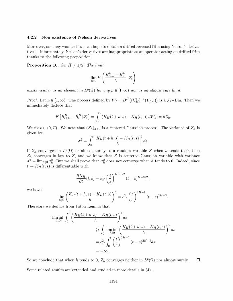
4.2.2 Non existence of Nelson derivatives

Moreover, one may wonder if we can hope to obtain a drifted reversed fBm using Nelson’s deriva-tives. Unfortunately, Nelson’s derivatives are inappropriate as an operator acting on drifted fBmthanks to the following proposition.

Proposition 10. Set H 6= 1/2. The limit

limh↓0

E

(BH

t+h −BHt

h

∣∣∣∣∣Ft

)

exists neither as an element in Lp(Ω) for any p ∈ [1,∞) nor as an almost sure limit.

Proof. Let p ∈ [1,∞). The process defined by Wt = BH((K∗

H)−1(1[0,t]))

is a Ft−Bm. Then weimmediately deduce that

E[BH

t+h −BHt |Ft

]=

∫ t

0(KH(t+ h, s) −KH(t, s)) dWs := hZh.

We fix t ∈ (0, T ). We note that (Zh)h>0 is a centered Gaussian process. The variance of Zh isgiven by:

σ2h =

∫ t

0

∣∣∣∣KH(t+ h, s) −KH(t, s)

h

∣∣∣∣2

ds.

If Zh converges in Lp(Ω) or almost surely to a random variable Z when h tends to 0, thenZh converges in law to Z, and we know that Z is centered Gaussian variable with varianceσ2 = limh↓0 σ

2h. But we shall prove that σ2

h does not converge when h tends to 0. Indeed, sincet 7→ KH(t, s) is differentiable with

∂KH

∂t(t, s) = cH

(t

s

)H−1/2

(t− s)H−3/2 ,

we have:

limh↓0

(KH(t+ h, s) −KH(t, s)

h

)2

= c2H

(t

s

)2H−1

(t− s)2H−3.

Therefore we deduce from Fatou Lemma that

lim infh↓0

∫ t

0


h

)2

ds

>

∫ t

0lim inf

h↓0


h

)2

ds

= c2H

∫ t

0

(t

s

)2H−1

(t− s)2H−3ds

= +∞ .

So we conclude that when h tends to 0, Zh converges neither in Lp(Ω) nor almost surely.

Some related results are extended and studied in more details in (4).

1194

4.2.3 The case H < 1/2

The techniques we have developed may provide a analogous theorem in the case H < 1/2, wheremoreover the formulas and the study of the operators K−1

H are more tractable. However, we lostthe structure of a ”drifted process” for the time reversed representation. As we will see in theproof of Theorem 9, we will construct in the case H > 1/2 a drift uH

· such that∫ ·0 usds = KH(g·),

where g is a process. Actually in the case H < 1/2, the operator KH does not map L2 into aspace of absolutely continuous functions (e.g. see (15) for the expressions of KH when H < 1/2).

So, although we can still write for YH

a continuous extension formula from the Wiener case:

YHt = Y

H0 + UH

t + BHt ,

the process UH is not in general of the form∫ ·0 u

Hs ds.

4.3 Proof of Theorem 9

In the sequel, we will use the letter XH for a semi-martingale driven by the Bm W , and bH todesign its drift. The notation XH means that the semi-martingale depends on H. We will haveX1/2 = Y 1/2.

We need the following lemma:

Lemma 11. Let X be a drifted Bm with drift (bt)t∈[0,T ] satisfying the assumptions of Theorem8:

Xt = x+

∫ t

0bsds+Wt , (28)

and let X its time reversed process:

X t = X0 +

∫ t

0bsds+ Wt.

Then for any 0 6 t 6 T , we have the following formula:∫ T−t

0KH(T − t, s)dXs = −

∫ T

T−tKH(T − t, T − u)dXu.

Proof. We first prove the following equality

∫ δ

γKH(T − t, s)dXs = −

∫ T−γ

T−δKH(T − t, T − u)dXu. (29)

where 0 < γ < δ < T − t. Remind that

KH(T − t, s) =(T − t− s)H−1/2

Γ (H + 1/2)F

(H − 1/2, 1/2 −H,H + 1/2, 1 − T − t

s

)

where F denotes Gauss hypergeometric function (see e.g. (6; 15)). The function z 7→F (H − 1/2, 1/2 −H,H + 1/2, z) is holomorphic on the domain z ∈ C, z 6= 1, |arg(1−z)| < π.It follows that the function

s 7→ F

(H − 1/2, 1/2 −H,H + 1/2, 1 − T − t

s

)

1195

is continuously differentiable on any interval [γ, δ], and so is the function s 7→ KH(T − t, s). Wededuce that s 7→ KH(T − t, s) is C1 on [γ, δ].

The integration by part formula w.r.t. the semimartingale X leads to

∫ δ

γKH(T − t, s)dXs = KH(T − t, δ)Xδ −KH(T − t, γ)Xγ −

∫ δ

γKH(T − t, s)Xsds.

With the definition of X and the change of variable u = T − t, we then write:

∫ δ

γKH(T − t, s)dXs = KH(T − t, δ)XT−δ −KH(T − t, γ)XT−γ

−∫ T−γ

T−δKH(T − t, T − u)Xudu.

We deduce (29) by the integration by part formula w.r.t. the semimartingale X .

To take the limit in (29) when (γ, δ) goes to (0, T − t), we write thanks to Theorem 5:

∫ δ

γKH(T − t, s)bsds +

∫ δ

γKH(T − t, s)dWs

= −∫ T−γ

T−δKH(T − t, T − u)budu−

∫ T−γ

T−δKH(T − t, T − u)dWu.

Since W and W are Brownian motion and s 7→ KH(T − t, s) ∈ L2(0, T ), we can take thedesired limit in the stochastic integrals. Moreover we also have s 7→ KH(T − t, s) ∈ Lq(0, T ) forq ∈ (2, 2/(2H − 1)) and b ∈ Lp(Ω × (0, T )) for p ∈ (1, 2), which concludes the proof.

Now we prove Theorem 9.

Proof. We divide the proof in two steps.

First step. Using the transfer principle and the isometry KH , it holds that

Y Ht = y +

∫ t

0KH(t, s)dXH

s

where

XHt = Wt +

∫ t

0K−1

H

(∫ ·

0uH

s ds

)(r)dr.

Thanks to the condition (i), we can apply Theorem 5 to the drifted Bm XH with finite energydrift process (bHt )t∈[0,T ] defined by

bHt = K−1H

(∫ ·

0uH

s ds

)(t) .

1196

If (Ft)t∈[0,T ] is the filtration generated by the reversed process XHt := XH

T−t, then there exists a

(Ft)-adapted processes (bHt )t∈[0,T ] ∈ Lp(Ω× [0, T ]) for any p ∈ (1, 2), and a (Ft)-Bm (WHt )t∈[0,T ]

such that

WHt = X

Ht −X

H0 −

∫ t

0bHs ds.

We deduce from Lemma 11 that

YHt = −

∫ T−t

0sH−1/2

(∫ s

0(s− r)H−3/2bHT−rr

1/2−Hdr

)ds

−∫ T

tKH(T − t, T − r)dWH

r .

We then write:

YHt − Y

H0 =

∫ t

0uH

s ds+ BHt ,

where

uHs = (T − s)H−1/2

(∫ T−s

0(T − s− r)H−3/2bHT−rr

1/2−Hdr

)

BHt =

∫ T

0KH(T, T − r)dWH

r −∫ T

tKH(T − t, T − r)dWH

r .

We compute the covariance of the centered Gaussian process (BHt )t∈[0,T ]:

E(BHs B

Ht ) =

⟨KH(T, T − ·),KH(T, T − ·)

⟩L2(0,T )

−⟨KH(T, T − ·),KH(T − s, T − ·)1[s,T ]

⟩L2(0,T )

−⟨KH(T − t, T − ·)1[t,T ],KH(T, T − ·)

⟩L2(0,T )

+⟨KH(T − t, T − ·)1[t,T ],KH(T − s, T − ·)1[s,T ]

⟩L2(0,T )

.

Since⟨KH(T − t, T − ·)1[t,T ],KH(T − s, T − ·)1[s,T ]

⟩L2(0,T )

=⟨KH(T − s, ·)1[0,T−s],KH(T − t, ·)1[0,T−t]

⟩L2(0,T )

=⟨1[0,T−t] , 1[0,T−s]

⟩H

= RH(T − t, T − s),

we deduce that

E(BHs B

Ht ) = RH(T, T ) −RH(T − s, T )

−RH(T, T − t) +RH(T − s, T − t)

= 1/2(2T 2H − |T − s|2H − T 2H + s2H − T 2H − |T − t|2H

+ t2H + |T − s|2H + |T − t|2H − |t− s|2H)

= RH(s, t) .

Hence the process (BHt )t∈[0,T ] is a fBm.

Remark moreover that writing the process uH· = OH (bT−·) shows that it is continuous (see (10)).

1197

Second step. Let us show that for all t ∈ (0, T ),∫ t0 u

Hs ds →

∫ t0 usds in L1(Ω) when H tends

to 1/2. We write∫ t

0(uH

s − us)ds =

∫ t

0OH

(bHT−· − uT−·

)(T − s)ds

+

∫ t

0(OH(uT−·)(T − s) − us) ds . (30)

First of all, we study the first term of the r.h.s. of (30). Lemma 1 implies that∣∣∣∣∫ t

0OH

(bHT−· − uT−·

)(T − s)ds

∣∣∣∣ 6

∫ T

0

∣∣∣OH

(bHT−· − uT−·

)(s)∣∣∣ ds

6 C(H0)

∫ T

0

∣∣∣bHT−s − uT−s

∣∣∣ s1/2−H0ds.

We have thanks to Proposition 7:

bHT−s − uT−s = limh↓0

E

[XH

s −XHs−h − (Xs −Xs−h)

h

∣∣∣FT−s

]

= limh↓0

E

[∫ ss−h(bHr − ur)dr

h

∣∣∣FT−s

]

= E[bHs − us

∣∣∣FT−s

].

So, by Jensen inequality and Fubini’s theorem

E

[∫ T

0s1/2−H0

∣∣∣bHT−s − uT−s

∣∣∣ ds]

6 E

[∫ T

0s1/2−H0

∣∣bHs − us

∣∣ ds]

and then

E

∣∣∣∣∫ t

0OH

(bHT−· − uT−·

)(T − s)ds

∣∣∣∣ 6

∫ T

0s1/2−H0E

∣∣bHs − us

∣∣ ds. (31)

We have

bHt − ut = K−1H

(∫ ·

0uH

s ds

)(t) − ut

and since

K−1H

(∫ ·

0uH

s ds

)(t) = tH−1/2D

H−1/20+ (s1/2−HuH

s )(t) ,

we get

∣∣bHt − ut

∣∣ 6∣∣∣∣∣t1/2−HuH

t

Γ(3/2 −H)− ut

∣∣∣∣∣

+t1/2−H(H − 1/2)

Γ(3/2 −H)

∣∣∣∣∣

∫ t

0

t1/2−HuHt − s1/2−HuH

s

(t− s)H+1/2ds

∣∣∣∣∣

6t1/2−H

Γ(3/2 −H)|uH

t − ut| +(

t1/2−H

Γ(3/2 −H)− 1

)|ut|

+t1/2−H(H − 1/2)

Γ(3/2 −H)

(I1(H, t) + I2(H, t)

)(32)

1198

where

I1(H, t) =

∫ t

0

t1/2−H |uHt − uH

s |(t− s)H+1/2

ds,

I2(H, t) =

∫ t

0

|uHs |(s1/2−H − t1/2−H)

(t− s)H+1/2ds.

Using E|uHt −uH

s | 6 C|t− s|η with η > H− 12 implies that E

(I1(H, t)

)is bounded uniformly for

(H, t) ∈ (1/2,H0)× (0, T ). From the inequality |t1/2−H − s1/2−H | 6 (H − 1/2)|t− s|(t/2)−1/2−H

for t > s > t/2 we deduce that

E(I2(H, t)

)6 c

∫ t

t2

(t− s)1/2−Hds + c

∫ t2

0(s1/2−H − t1/2−H)(t− s)1/2−Hds (33)

and E(I2(H, t)

)is also bounded uniformly in (H, t). Now, since E|uH

t −ut| tends to 0 as H ↓ 1/2we have

E∣∣bHt − ut

∣∣ −→ 0 as H ↓ 12 for almost all t. (34)

Let 1 < p < 1H0

< 2, we use Holder inequality

∫ T

0sp(1/2−H0)E|bHs − us|pds 6

(∫ T

0s

2p( 12−H0)

2−p ds

) 2−p2(E

∫ T

0|bHs − us|2ds

) p2

.

Thanks to the hypothesis (ii), s 7→ s1/2−H0E|bHs − us| ; H ∈ [1/2,H0] is bounded inLp([0, T ], dt

T

), thus this family is uniformly integrable.

By (34),s1/2−H0E|bHs − us| → 0 , ds

T a.s.

when H tends to 1/2, so this convergence also holds in L1([0, T ], dt

T

). Reporting this convergence

result in (31),

E

∣∣∣∣∫ t

0OH (bHT−· − uT−·)(T − s)ds

∣∣∣∣ −→ 0

when H tends to 1/2.

We now study the second term of the r.h.s. of (30). We write:∫ t

0OH(uT−·)(T − s)ds =

∫ T

T−tOH(uT−·)(r)dr

= KH(uT−·)(T ) −KH(uT−·)(T − t).

By Theorem 5, u ∈ Lp(0, T ) a.s. for any p ∈ (1, 2), and consequently u satisfies a.s. thehypothesis of Lemma 1 which then yields the following estimation and convergence:

∣∣∣∣∫ t

0OH (uT−·) (T − s)ds

∣∣∣∣ 6

∫ T

0|OH (uT−·) (s)| ds

6 C(H0)

∫ T

0|uT−s|

(s1/2−H0 ∨ 1

)ds,

limH↓1/2

∫ t

0OH(uT−·)(T − s)ds =

∫ T

0uT−rdr −

∫ T−t

0uT−rdr

=

∫ t

0usds a.s.

1199

Since for any p ∈ (1, 2), u ∈ Lp(Ω × (0, T )), we have

∫ T

0|uT−s| (s1/2−H0 ∨ 1)ds ∈ L1(Ω),

and we can apply the dominated convergence theorem and write

limH↓1/2

E

∣∣∣∣∫ t

0OH(uT−·)(T − s)ds−

∫ t

0usds

∣∣∣∣ = 0.

So we conclude that for all t ∈ (0, T ),∫ t0 u

Hs ds→

∫ t0 usds in L1(Ω) when H tends to 1/2.

Using Lemma 3.2 in (5), we have

E|BHt −Wt|2 6 (cT )2|H − 1/2|2

and then BHt tends to Wt in L2(Ω) when H tends to 1/2.

Since YHt = Y H

T−t = y +∫ T−t0 uH

s ds+BHT−t we deduce that Y

Ht tends to Y

1/2t in L1(Ω) when H

tends to 1/2. Hence, for all t ∈ (0, T )

limH↓1/2

BHt = Wt in L1(Ω),

which concludes the proof of the theorem.

5 Application to stochastic differential equations driven by a

fBm

First of all, we apply our result to the reversal of a fBm. We yet consider that BH is a fBmhaving the integral representation BH

t =∫ t0 KH(t, s)dWs. It is well known (see (17)) that the

reversed process W solves:

dW t = − W t

T − tdt+ dWt,

where the Brownian motion Wt is given by

Wt = WT−t −WT +

∫ T

T−t

Ws

sds.

Therefore, thanks to Theorem 9, we deduce that the reversed fBm reads:

BHt = B

H0 +

∫ t

0(T − s)H−1/2

∫ T−s

0r−1/2−H(T − s− r)H−3/2Wrdrds+ BH

t

where the fBm (BHt )t∈[0,T ] is given by

BHt =

∫ T

0KH(T, T − u)dWu −

∫ T

tKH(T − t, T − u)dWu.

This situation can be extended in the case of stochastic differential equations driven by BH .

1200

5.1 SDE driven by a single fBm

Using successively Theorem 9, Theorem 8 and the results in (17), we can state the followingproposition:

Proposition 12. (a) Let Y H be the process defined as the unique solution of

Y Ht = y +

∫ t

0u(Y H

s )ds +BHt , 0 6 t 6 T , (35)

where the function u is bounded with bounded first derivative. Then there exists a family of pro-

cesses(uH)H>1/2

and a family of fBm (BH)H>1/2 such that the time reversed process (YHt )t∈[0,T ]

defined by YHt = Y H

T−t satisfies

YHt = Y

H0 +

∫ t

0uH

s ds+ BHt ,

with the following L1(Ω) convergences

limH↓1/2

BHt = B

1/2T −B

1/2T−t +

∫ T

T−t∂x log ps(Y

1/2s ) ds = B

1/2t , (36)

limH↓1/2

∫ t

0uH

s ds =

∫ t

0

(−u(Y 1/2

s ) + ∂x log pT−s(Y1/2s )

)ds (37)

for all t ∈ (0, T ), where (t, y) 7→ pt(y) is the density of the law of Y1/2t solution of

Y1/2t = y +

∫ t

0u(Y 1/2

s )ds+B1/2t .

(b) The process YH

is not a ”fractional diffusion”, i.e. of the form (12).

Proof. It is proved in (15) that there exists a unique strong solution of stochastic differentialequation (35).

First step. In order to prove (a), we have to verify that all the assumptions of Theorem 9are fulfilled. We recall that

bHt = K−1H

(∫ ·

0u(Y H

s )ds

)(t).

The process (bHt )t∈[0,t] satisfies the Novikov condition (16) as noticed in the section 3.3 p.110−111in (15) and the condition (i) holds true.

We check the assumptions of (ii).

The trajectories of the process (Yt)t∈[0,T ] are Holder continuous of order H − ǫ for all ǫ > 0(see (16; 15)). Since the function u has a bounded first derivative, the process (u(Yt))t∈[0,T ] has

1201

Second step. We now prove (b). We have to use Theorem 8 to obtain the explicit form ofthe drift. In order to verify the conditions 1, 2 and 3 of Theorem 8, we compute the Malliavinderivatives with respect to the process (Xt)t∈[0,T ] defined by

Xt = Wt +

∫ t

0K−1

H

(∫ ·

0u(Ys)ds

)(r)dr

which is a Bm under the probability measure Q defined by dQ/dP = G where G is given by(20). Let Yt =

∫ t0 KH(t, s)dXs where we omit the index H for Y for simplicity. In view of the

form of Y , (Yt)t∈[0,T ] is a fBm with respect to the new probability measure Q and we have thefollowing relations between the Malliavin derivative with respect to X (denoted by D) and theMalliavin derivative with respect to Y (denoted DY ): for any random variable F ∈ D1,2

K∗H

(DY F

)= DF .

Let α = H − 1/2, using (9) one writes

bt = tαDα0+

(s−αu(Ys)

)(t)

=1

Γ(1 − α)

(t−αu(Yt) + αtα

∫ t

0

t−αu(Yt) − s−αu(Ys)

(t− s)α+1ds

),

and one remarks that for any r 6 t

DYr bt =

1

Γ(1 − α)

(t−αu′(Yt)1r6t

+ αtα∫ t

0

t−αu′(Yt)1r6t − s−αu′(Ys)1r6s

(t− s)α+1ds).

The following computations are quite the same one that those carried out in the proof of Lemma14 of (11) in a different framework. For sake of completeness, we include them.

Drbt =1

Γ(1 − α)

(t−αu′(Yt)K∗

H

(1[0,t]

)(r)

+ αtα∫ t

0

t−αu′(Yt)K∗H

(1[0,t]

)(r) − s−αu′(Ys)K∗

H

(1[0,s]

)(r)

(t− s)α+1ds)

=1

Γ(1 − α)

(t−αu′(Yt)KH(t, r)1r6t

+ αtα∫ t

0

t−αu′(Yt)KH(t, r)1r6t − s−αu′(Ys)KH(s, r)1r6s

(t− s)α+1ds)

:= f1(t, r) + f2(t, r) + f3(t, r) + f4(t, r),

where

f1(t, r) =1

Γ(1 − α)u′(Yt)KH(t, r)(t− r)−α

f2(t, r) =αu′(Yt)

Γ(1 − α)

∫ t

r

KH(t, r) −KH(s, r)

(t− s)α+1ds

f3(t, r) =α

Γ(1 − α)

∫ t

r

u′(Yt) − u′(Ys)

(t− s)α+1KH(s, r)ds

f4(t, r) =αtα

Γ(1 − α)

∫ t

r

t−α − s−α

(t− s)α+1u′(Ys)KH(s, r)ds

1203

for r 6 t and the functions fi, i = 1, ..., 4 vanish when r > t. Remind that (see (3)) that

KH(t, r) = cH(H − 1/2

)r−α

∫ t

r(θ − r)α−1θαdθ , (39)

we have

f2(t, r) =cHα

2

Γ(1 − α)u′(Yt)

∫ t

r

r−α∫ ts (θ − r)α−1θαdθ

(t− s)α+1ds

=cHα

2

Γ(1 − α)u′(Yt)r

−α

∫ t

r

∫ θ

r(t− s)−α−1ds(θ − r)α−1θαdθ

= f5(t, r) − f1(t, r) with

f5(t, r) =cHα

Γ(1 − α)u′(Yt)r

−α

∫ t

r(t− θ)−α(θ − r)α−1θαdθ,

and it follows thatDrbt = f3(t, r) + f4(t, r) + f5(t, r). (40)

The above expression implies that the process (Drbt)t∈[0,T ] is adapted with respect to the fil-tration generated by the Bm X because it is the same one that the filtration generated by theprocess Y . Therefore if we have

EQ

∫ T

0

∫ T

0|Drbt|2drdt <∞ , (41)

the assumptions 1, 2 and 3 of Theorem 8 will be checked.

Using the fact that (Yt)t∈[0,T ] is a fBm under the probability Q and Lemma 2, we get that forany ǫ > 0, there exists a square integrable random variable ζH,ǫ such that

|Yt − Ys| 6 ζH,ǫ|t− s|H−ǫ.

Since the function u is Lipschitz, we get for 0 < ǫ < 1/2

EQ

∫ T

0

∫ T

0|f3(t, r)|2drdt 6 EQ

∫ T

0

∫ T

0c ζ2

H,ǫ

∣∣∣∣∫ t

r(t− s)−

12−ǫKH(s, r)ds

∣∣∣∣2

drdt .

Reporting in the expression (39) the fact that θα 6 rα for θ > r yields

|KH(s, r)| 6 cH(s− r)α. (42)

We conclude that

EQ

∫ T

0

∫ T

0|f3(t, r)|2drdt 6 c <∞. (43)

From the inequalities (42) and |t−α − s−α| 6 α(t− s)t−α+1 for t > s > r, we get

|f4(t, r)| 6αcH‖u′‖∞Γ(1 − α)

tα∫ t

r

t−α−1

(t− s)α(s− r)αds 6 c t−1

∫ t

r

(s− r

t− s

)α

ds ,

1204

and the change of variable s = (t− r)ξ + r yields

|f4(t, r)| 6 c t−1(t− r)

∫ 1

0ξα(1 − ξ)−αdξ 6 c β(1 − α,α+ 1) .

We finally get

EQ

∫ T

0

∫ T

0|f4(t, r)|2drdt <∞. (44)

We use another time the inequality θα 6 rα for θ > r and the change of variable θ = (t− r)ξ+ rin order to have

|f5(t, r)| 6αcH‖u′‖∞Γ(1 − α)

(t− r)1−αβ(1 − α,α) ,

and consequently

EQ

∫ T

0

∫ T

0|f5(t, r)|2drdt <∞. (45)

The expression (40) and the inequalities (43), (44) and (45) imply that (41) is satisfied. Con-sequently, Theorem 8 asserts that there exists a reversed drift b of the form (21) for the time

reversal of X. Since the drift uH of YH

reads uH· = OH (bT−·), we deduce that Y

Hcannot be a

”fractional diffusion”.

5.2 A remark on fractional SDE with a non linear diffusion coefficient

We are now interested in fractional SDE with a non linear diffusion coefficient. Let XH be thesolution of

XHt = x0 +

∫ t

0σ(XH

s )dBHs +

∫ t

0b(XH

s ) ds, t ∈ [0, T ], (46)

where the stochastic integral is understood in the Young sense.

Let us assume the conditions given in (10) to ensure that the time reversed process of thediffusion X1/2 is again a diffusion:

1. b : R → R and σ : R → R are Borel measurable functions satisfying the hypothesis: thereexists a constant K > 0 such that for every x, y ∈ R we have

|σ(x) − σ(y)| + |b(x) − b(y)| 6 K |x− y| ,|σ(x)| + |b(x)| 6 K(1 + |x|).

2. For any t ∈ (0, T ), X1/2t has a density pt.

3. For any t0 ∈ (0, T ), for any bounded open set O ⊂ R,

∫ T

t0

∫

O

∣∣∂x(σ2(x)pt(x))∣∣ dxdt < +∞.

1205

Moreover, assume that |σ| ≥ c > 0 does not vanish. As in (15) we set Y Ht = h(XH

t ) whereh(x) =

∫ x0

dyσ(y) . Using the change of variables formula, we obtain that Y verifies

Y Ht = y0 +BH

t +

∫ t

0

b(h−1(Y Hs ))

σ(h−1(Y Hs ))

ds, t ∈ [0, T ].

If b and σ are such that b h−1/σ h−1 is bounded with bounded first derivative, we can apply

our previous theorem and obtain a time reversed representation for YHt (which is continuous in

L1(Ω) when H ↓ 1/2):

YHt = Y

H0 +

∫ t

0uH

s ds+ BHt .

But XHt = h−1(Y

Ht ), so:

XHt = X

H0 +

∫ t

0σ(X

Hs )uH

s ds+

∫ t

0σ(X

Hs )dBH

s .

If we assume that σ is bounded, the derivative of h−1 will also be bounded, hence XHt is

continuous in L1(Ω) when H ↓ 1/2. Those of∫ t0 σ(X

Hs )uH

s ds is ensured by uH ∈ Lp(Ω × [0, T ])

for p ∈ (1, 2) and σ Lipschitz. As a consequence, the stochastic integral∫ t0 σ(X

Hs )dBH

s is alsocontinuous in L1(Ω) when H ↓ 1/2.

6 H-deformation of Nelson derivatives

In this section we explore one possible way to construct dynamical operators acting on diffusionsdriven by a fractional Brownian motion.

For 1/2 6 H < 1 we denote by ΥHy the vector space of all processes Y H of the form

Y Ht = y +

∫ t

0uH

s ds+ σBHt ,

where σ ∈ R and (uHt )t∈[0,T ] is a Ft-adapted squared integrable process such that the process

bH := K−1H

(∫ ·0 u

Hs ds

)satisfies the Novikov condition (16) and the conditions 1, 2 and 3 of

Theorem 8,

In particulary, Υ1/20 is the space of all drifted Bm starting from 0 with a constant diffusion

coefficient and a Ft-adapted square integrable drift satisfying (16).

The following map is then well defined:

TH :

Υ1/20 −→ ΥH

y

X 7−→ y +

∫ ·

0KH(·, s)dXs

Let Y H ∈ ΥHy be of the form Y H

t = y +∫ t0 u

Hs ds + σBH

t , then clearly TH(X) = Y with

Xt =∫ t0 K−1

H (∫ ·0 usds)(r)dr + σWt, so TH is surjective. Assume moreover that TH(X) = 0 with

Xt =∫ t0 bsds + σWt. Thus TH(X)t = y +

∫ t0 usds + σBH

t = 0 with u(s) = KH(b)(s). Since BH

1206

is not absolutely continuous, this implies that σ = 0. By differentiating, we obtain u = 0. SoX = 0 and TH is one to one. Consequently, the application TH is an isomorphism.

In the case H = 1/2, the drift of an element of Υ1/2W has a dynamical meaning in the sense of

Nelson (c.f. Proposition 7). The isomorphism TH provides us a way to introduce an equivalentnotion in the general case H ∈ (1/2, 1).

Definition 13. Let Y ∈ ΥHBH with H ∈ (1/2, 1). The quantities

DH

+Yt = OH D+ T−1H (Y )t,

DH

−Yt = OH D− T−1H (Y )t

are well defined and respectively called the H-forward Nelson and H-backward Nelson derivativeof Y at time t.

The fact that these operators are well defined is a consequence of Theorem 9, and moreover wehave for all t ∈ (0, T ),

ut = DH

+Yt.

So we have constructed an operator which associates to a process Y ∈ ΥHBH its drift. However

this operator does not calculate a difference rate directly on the process Y involved, but via atransfer principle. Moreover the map TH hides difficulties as regards explicit calculation.

A Appendix

A.1 Proof of Theorem 5

Proof. Set dQ = G · dP where

G = exp

(−∫ T

0bsdWs − 1/2

∫ T

0b2sds

).

Since b fulfills the Novikov condition, the Girsanov theorem shows that (Xt)t∈[0,T ] is a (Ft,Q)-Bm.

Lemma 14. Let (Ft) be the natural filtration generated by X. Then the process (W(1)t )t∈[0,T ]

defined by

W(1)t := X t −X0 −

∫ t

0

Xr

T − rdr

is a (Ft,Q)-Bm.

Proof. We have

W(1)t = XT−t −XT +

∫ t

0

XT−r

T − rdr.

We write Fs = σ(XT−s) ∨ GT−s where GT−s = σ(Xr −Xr′ , T − s 6 r < r′ 6 T ). For s < t, wehave:

EQ

[W

(1)t −W (1)

s

∣∣∣Fs

]= EQ

[XT−t −XT−s

∣∣∣Fs

]+

∫ t

s

EQ[XT−r|Fs]

T − rdr.

1207

But XT−t − XT−s is independent of GT−s and for all r ∈ [s, t], XT−r = XT−r − X0 is alsoindependent of GT−s. Therefore:

EQ

[W

(1)t −W (1)

s

∣∣∣Fs

]= EQ [XT−t −XT−s |XT−s ] +

∫ t

s

EQ [XT−r |XT−s ]

T − rdr.

Since (Xt)t∈[0,T ] is a Q-Bm and EQ [(XT−u − α(u)XT−s)XT−s] = 0, we can write

EQ [XT−u −XT−s |XT−s ] = α(u)XT−s =T − u

T − sXT−s

Thus

EQ

[W

(1)t −W (1)

s

∣∣∣Fs

]=

[T − t

T − s− 1 +

∫ t

s

dr

T − s

]XT−s = 0.

andW (1) is a (Ft,Q)-martingale. The fact that the quadratic variation of the continuous (Ft,Q)-martingale W (1) is equal to t together with Levy theorem conclude the proof of the lemma.

Since P ∼ Q, Girsanov theorem insures the existence of a (Ft)-adapted process (at)t∈[0,T ] suchthat

Wt := W(1)t −

∫ t

0asds

is a (Ft,P)-Bm. The process (at)t∈[0,T ] has finite energy with respect to P which has finiteentropy with respect to Q (see Lemma 3.1 in (7)).We then write

Wt = X t −X0 −∫ t

0bsds

where

bs = as +Xs

T − s(47)

is a (Fs)-adapted process with a priori only local finite energy, namely finite energy on any timeinterval [0, τ ] for τ < T .

However, one can prove that b ∈ Lp(Ω × [0, T ]), 1 < p < 2. The expression (47) indeed gives:

|bT−s| 6 |aT−s| +1

s

(|Ws| +

∫ s

0|br|dr

)

6 |aT−s| +1

s

(|Ws| +

√s

√∫ s

0|br|2dr

).

For any p ∈ (1, 2), Wss ∈ Lp(Ω × [0, T ]). Finally, with

∫ T0 s−p/2ds < ∞, b ∈ L2(Ω × [0, T ])

and the Jensen inequality applied with the convex function x 7→ x2/p, one can deduce thatb ∈ Lp(Ω × [0, T ]).

1208

A.2 Proof of Theorem 8

Proof. We follow the ideas of Follmer.

We denote Gt = FT−t = σXu ; t 6 u ≤ T = F[t,T ]∨σXt, where F[t,T ] denotes the sigma-fieldgenerated by the increments of the Bm X between t and T .

Remind that the drift (bt)t∈[0,T ] can be expressed in term of forward Nelson derivative. Thereversed drift is expressed thanks to (backward) Nelson derivative:

bT−t = − limh↓0

E

(Xt −Xt−h

h

∣∣∣∣Gt

)in L2(Ω) . (48)

We introduce the following subset of L2(Ω):

Tt0 =

exp

(αXt0 +

∫ T

t0

hsdXs

); α ∈ R, h ∈ L2(0, T )

.

It is easy to check that Tt0 is a total subset of L2(Ω,Gt0 ,Q).

Then, in order to compute the conditional expectation (48), we have to compute

limh→0+

1

hE (F (Xt0 −Xt0−h))

for any random variable F in Tt0 . It is straightforward that for all t 6 t0, Dt0F = DtF .

We now write for all square integrable deterministic function ht:

E

[F

∫ T

0htdXt

]= EQ

[G−1F

∫ T

0htdXt

]

= EQ

[G−1

∫ T

0DtF.htdt

]+ EQ

[F

∫ T

0Dt(G

−1).htdt

]

= E

[∫ T

0DtF.htdt

]+ E

[GF

∫ T

0Dt(G

−1).htdt

].

using G−1 = exp

(∫ T

0bsdXs − 1/2

∫ T

0b2sds

)and the commutativity relationship between the

Malliavin derivative and the stochastic integral (see (13), p.38) yield

G.Dt(G−1) = bt +

∫ T

tDtbsdXs −

∫ T

0bs.Dtbsds

= bt +

∫ T

tDtbsdWs.

Taking ht = 1[t0−h,t0](t), we thus obtain:

E[F (Xt0 −Xt0−h)] = E

[∫ t0

t0−hDtFdt

]+ E

[F

∫ t0

t0−h

(bt +

∫ T

tDtbsdWs

)dt

].

Since F ∈ Tt0 , we have

E[F (Xt0 −Xt0−h)] = hE [Dt0F ] + E

[F

∫ t0

t0−h

(bt +

∫ T

tDtbsdWs

)dt

]. (49)

1209

With

E[bT−t0F

]= − lim

h→0+

1

hE[F (Xt0 −Xt0−h)] ,

we deduce that

− E[bT−t0F

]= E [Dt0F ] + E

[F

(bt0 +

∫ T

t0

Dt0bsdWs

)]. (50)

From (49), we write:

E [Dt0F ] =1

t0E

[F

(Xt0 −

∫ t0

0

(bt +

∫ T

tDtbsdWs

)dt

)]

=1

t0E

[F

(Wt0 −

∫ t0

0

∫ T

tDtbsdWsdt

)].

Using (49), we conclude that:

− E[(bT−t0 + bt0)F

]= E

[F

(∫ T

t0

Dt0bsdWs

+1

t0

(Wt0 −

∫ t0

0

∫ T

tDtbsdWsdt

))],

and the formula for the reversed drift (21) is proved.

Acknowledgment: We want to thank the anonymous referee for a careful and thorough readingof this work and his constructive remarks.

References

[1] Alos, E. and Nualart, D. Stochastic Integration with respect to the fractional Brownian Mo-tion. Stochastics and stochastics Reports 75, 129-152 (2003). MR1978896

[2] Carmona, P. Coutin, L. and Montseny, G.: Stochastic Integration with respect to the frac-tional Brownian Motion. Ann. Inst. H. Poincare Probab. Statist. 39, no. 1, 27-68 (2003).MR1959841

[3] Cresson J., Darses S.: Plongement stochastique des systemes lagangiens. C.R. Acad. Sci.Paris, Ser. I 342 (2006). MR2201959

[4] Darses S., Nourdin I. : Stochastic derivatives for fractional diffusions. Ann. Prob. To appear.

[5] Decreusefond, L.: Stochastic integration with respect to Volterra processes. Ann. Inst. H.Poincare Probab. Statist. 41, no. 2, 123-149 (2005). MR2124078

[6] Decreusefond, L. and Ustunel, A.S.: Stochastic Analysis of the Fractional Brownian Motion.Potential Analysis 10, no.2, 177-214 (1999). MR1677455

[7] Follmer, H.: Time reversal on Wiener space. In Stochastic processes, mathematics andphysics (Bielefeld, 1984). Lecture Notes in Math. Vol 1158, 119-129 (1986). MR0838561

1210

http://www.ams.org/mathscinet-getitem?mr=1978896






[8] Garsia, A., Rodemich, E. and Rumsey, H.: A real variable lemma and the continuity of pathsof some Gaussian processes. Indiana Univ. Math. Journal 20, 565-578 (1970/71). MR0267632

[9] Haussmann, U.G., Pardoux, E.: Time reversal of diffusions. Ann. Prob. 14, no.4, 1188-1205(1986). MR0866342

[10] Millet, A., Nualart, D., Sanz, M.: Integration by parts and time reversal for diffusionprocesses. Ann. Prob. 17, 208-238 (1989). MR0972782

[11] Moret, S. and Nualart, D.: Onsager-Machlup functional for the fractional Brownian motion.Prob. Theory Related Fields 124, 227-260 (2002). MR1936018

[12] Nelson, E.: Dynamical theory of Brownian motion. Princeton University Press(1967).MR0214150

[13] Nualart, D.: The Malliavin Calculus and Related Topics. Springer Verlag (1996).

[14] Nualart, D.: Stochastic calculus with respect to the fractional Brownian motion and appli-cations. Contemporary Mathematics 336, 3-39 (2003). MR2037156

[15] Nualart, D. and Ouknine, Y.: Regularization of differential equations by fractional noise.Stochastic Processes and their Applications 102, 103-116 (2002). MR1934157

[16] Nualart, D. and Rascanu, A.: Differential Equations driven by fractional Brownian motion.Collect. Math. 53, 1, 55-81 (2002). MR1893308

[17] Pardoux, E.: Grossissement d’une filtration et retournement du temps d’une diffusion.Seminaire de Probabilites, XX, 1984/85, 48-55, Lecture Notes in Math., 1204, Springer,Berlin (1986). MR0942014

1211










Time reversal for drifted fractional Brownian motion with ...

Documents

Transcript of Time reversal for drifted fractional Brownian motion with ...