ISM 270

Service Engineering and Management

Lecture 6: Forecasting

Vijay Mehrotra

Director and Associate Professor, San Francisco University

Author of regular column ‘Analyze This!’ in Analytics Magazine

Former CEO of Onward, Inc, which became part of Blue Pumpkin and Advertising.com

Ph.D. Stanford, 1992

Announcements

Homework 3 due today Project proposal due next week Next week: Qing Wu, Google

Forecasting Demand for Services

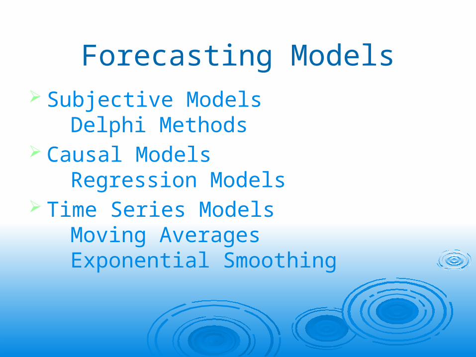
Forecasting Models Subjective Models

Delphi Methods Causal Models

Regression Models Time Series Models

Moving AveragesExponential Smoothing

Delphi ForecastingQuestion: In what future election will a woman become president of the united states for

the first time?

Year 1st Round Positive Arguments 2nd Round Negative Arguments 3rd Round

2008

2012

2016

2020

2024

2028

2032

2036

2040

2044

2048

2052

Never

Total

N Period Moving Average

Let : MAT = The N period moving average at the end of period T AT = Actual observation for period T

Then: MAT = (AT + AT-1 + AT-2 + …..+ AT-N+1)/N

Characteristics: Need N observations to make a forecast Very inexpensive and easy to understand Gives equal weight to all observations Does not consider observations older than N periods

Moving Average Example

Saturday Occupancy at a 100-room Hotel

Three-period Saturday Period Occupancy Moving Average Forecast

Aug. 1 1 79 8 2 84 15 3 83 82 22 4 81 83 82 29 5 98 87 83Sept. 5 6 100 93 87 12 7 93

Exponential Smoothing

Let : ST = Smoothed value at end of period T AT = Actual observation for period T FT+1 = Forecast for period T+1

Feedback control nature of exponential smoothing

New value (ST ) = Old value (ST-1 ) + [ observed error ]

S S A S

S A S

F S

T T- T T

T T T

T T

1 1

1

1

1

[ ]

( )or :

Exponential SmoothingHotel Example

Saturday Hotel Occupancy ( =0.5) Actual Smoothed Forecast Period Occupancy Value Forecast ErrorSaturday t At St Ft |At - Ft|Aug. 1 1 79 79.00 8 2 84 81.50 79 5 15 3 83 82.25 82 1 22 4 81 81.63 82 1 29 5 98 89.81 82 16Sept. 5 6 100 94.91 90 10

Mean Absolute Deviation (MAD) = 6.6 Forecast Error (MAD) = ΣlAt – Ftl/n

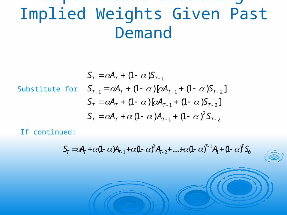
Exponential SmoothingImplied Weights Given Past Demand

S A S

S A A S

S A A S

S A A S

T T T

T T T T

T T T T

T T T T

( )

( )[ ( ) ]

( )[ ( ) ]

( ) ( )

1

1 1

1 1

1 1

1

1 1 2

1 2

12

2

Substitute for

If continued:

S A A A A ST T T TT T ( ) ( ) ..... ( ) ( )1 1 1 11

22

11 0

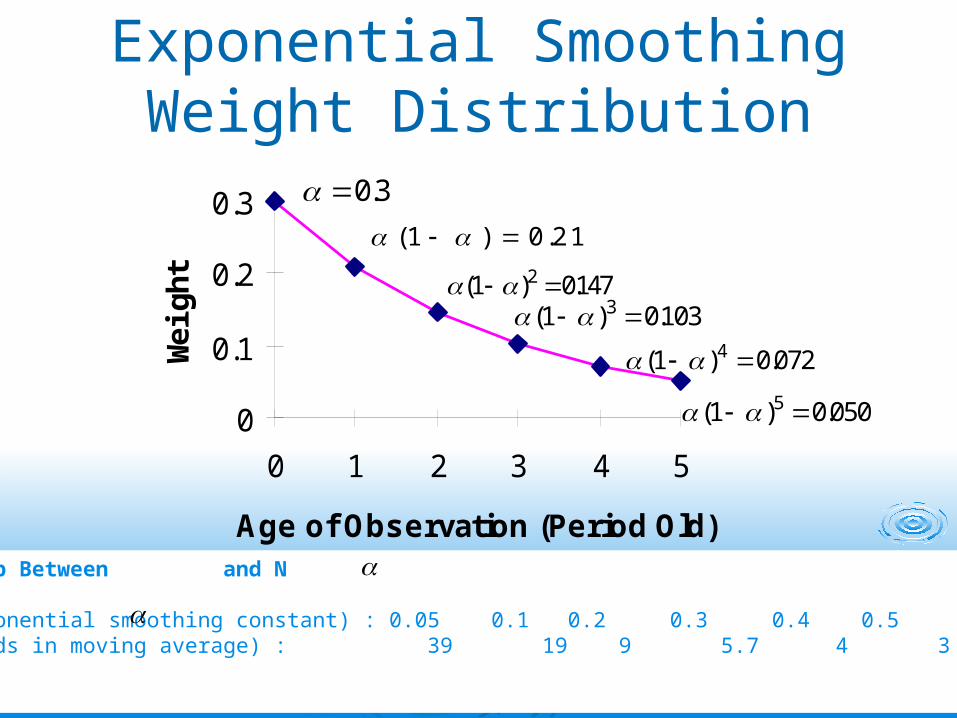
Exponential Smoothing Weight Distribution

0

0.1

0.2

0.3

0 1 2 3 4 5

Age of Observation (Period Old)

Wei

ght

0 3.

( ) .1 0 21

( ) .1 01472 ( ) .1 01033

( ) .1 0 0724

( ) .1 0 0505

Relationship Between and N

(exponential smoothing constant) : 0.05 0.1 0.2 0.3 0.4 0.5 0.67 N (periods in moving average) : 39 19 9 5.7 4 3 2

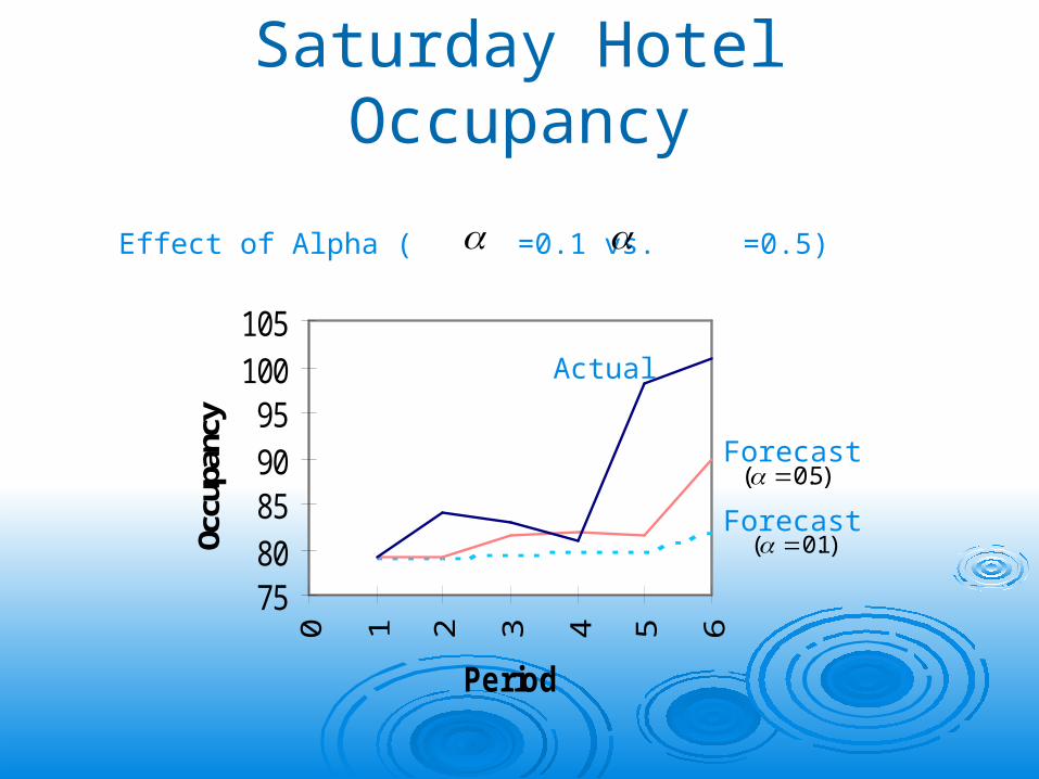
Saturday Hotel Occupancy

Effect of Alpha ( =0.1 vs. =0.5)

7580859095

100105

0 1 2 3 4 5 6Period

Occ

upan

cy

Actual

Forecast

Forecast

( . ) 05

( . ) 01

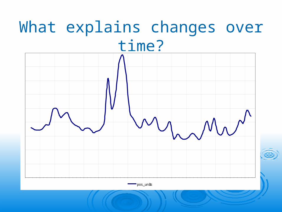
What explains changes over time?

pos_units

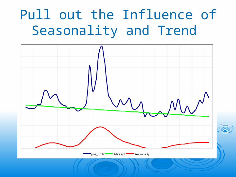
Pull out the Influence of Seasonality and Trend

pos_units Intercept Seasonality

Estimate the relationship of price and promotion changes to volume

pos_units Intercept Seasonality Holiday Price Change Ad Display

Ad Flag

Display Flag

Base Price

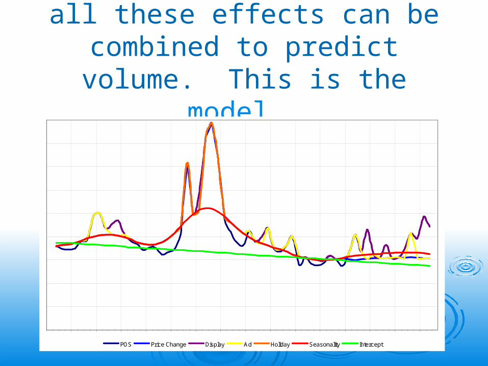
Once estimated separately, all these effects can be combined to

predict volume. This is the model.

POS Price Change Display Ad Holiday Seasonality Intercept

Exponential Smoothing With Trend Adjustment

S A S T

T S S T

F S T

t t t t

t t t t

t t t

( ) ( )( )

( ) ( )

1

11 1

1 1

1

Commuter Airline Load Factor

Week Actual load factor Smoothed value Smoothed trend Forecast Forecast error t At St Tt Ft | At - Ft|

1 31 31.00 0.00 2 40 35.50 1.35 31 9 3 43 39.93 2.27 37 6 4 52 47.10 3.74 42 10 5 49 49.92 3.47 51 2 6 64 58.69 5.06 53 11 7 58 60.88 4.20 64 6 8 68 66.54 4.63 65 3 MAD = 6.7

( . , . ) 05 0 3

Exponential Smoothing with Seasonal Adjustment

S A I S

F S I

IA

SI

t t t L t

t t t L

tt

tt L

( / ) ( )

( )( )

( )

1

1

1

1 1

Ferry Passengers taken to a Resort Island Actual Smoothed Index Forecast ErrorPeriod t At value St It Ft | At - Ft| 2003January 1 1651 ….. 0.837 ….. February 2 1305 ….. 0.662 ….. March 3 1617 ….. 0.820 …..April 4 1721 ….. 0.873 ….. May 5 2015 ….. 1.022 …..June 6 2297 ….. 1.165 ….. July 7 2606 ….. 1.322 ….. August 8 2687 ….. 1.363 ….. September 9 2292 ….. 1.162 …..October 10 1981 ….. 1.005 …..November 11 1696 ….. 0.860 …..December 12 1794 1794.00 0.910 ….. 2004January 13 1806 1866.74 0.876 - - February 14 1731 2016.35 0.721 1236

495March 15 1733 2035.76 0.829 1653 80

( . , . ) 0 2 0 3

More sophisticated forecasting techniques

Nonlinear Regression Data mining Machine Learning Simulation-based

Managing Service Projects

The Nature of Project Management

Characteristics of Projects: purpose, life cycle, interdependencies, uniqueness, and conflict.

Project Management Process: planning (work breakdown structure), scheduling, and controlling.

Selecting the Project Manager: credibility, sensitivity, ability to handle stress, and leadership.

Building the Project Team: Forming, Storming, Norming, and Performing.

Principles of Effective Project Management: direct people individually and as a team, reinforce excitement, keep everyone informed, manage healthy conflict, empower team, encourage risk taking and creativity.

Project Metrics: Cost, Time, Performance

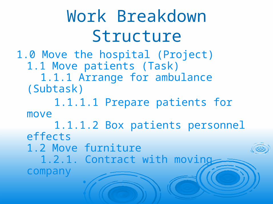
Work Breakdown Structure

1.0 Move the hospital (Project)1.1 Move patients (Task)

1.1.1 Arrange for ambulance (Subtask)1.1.1.1 Prepare patients for move1.1.1.2 Box patients personnel

effects1.2 Move furniture

1.2.1. Contract with moving company•••

Project Management Questions

What activities are required to complete a project and in what sequence?

When should each activity be scheduled to begin and end?

Which activities are critical to completing the project on time?

What is the probability of meeting the project completion due date?

How should resources be allocated to activities?

Example: Planning a Tennis Tournament

What is the earliest / latest each activity can be begin / be completed?

Given the plan, how likely is it that things will run behind schedule?

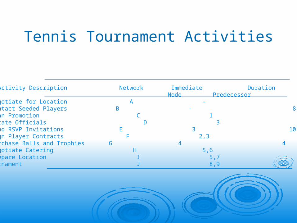
Tennis Tournament Activities

ID Activity Description Network Immediate Duration Node Predecessor (days)1 Negotiate for Location A - 22 Contact Seeded Players B - 83 Plan Promotion C 1 34 Locate Officials D 3 25 Send RSVP Invitations E 3 106 Sign Player Contracts F 2,3 47 Purchase Balls and Trophies G 4 48 Negotiate Catering H 5,6 19 Prepare Location I 5,7 310 Tournament J 8,9 2

Notation for Critical Path Analysis

Item Symbol Definition

Activity duration t The expected duration of an activity

Early start ES The earliest time an activity can begin if all previous activities are begun at their earliest times

Early finish EF The earliest time an activity can be completed if it is started at its early start time

Late start LS The latest time an activity can begin without delaying the completion of the project

Late finish LF The latest time an activity can be completed if it is started at its latest start time

Total slack TS The amount of time an activity can be delayed without delaying the completion of the project

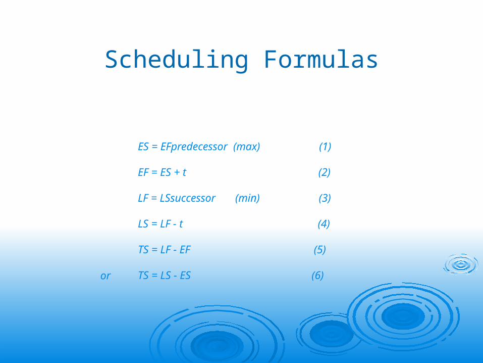
Scheduling Formulas

ES = EFpredecessor (max) (1)

EF = ES + t (2)

LF = LSsuccessor (min) (3)

LS = LF - t (4)

TS = LF - EF (5)

TS = LS - ES (6) or

Tennis Tournament Activity on Node Diagram

J2

B8

START

A2 C3 D2 G4

E10 I3

F4 H1

TS ES EF

LS LF

Early Start Gantt Chart for Tennis Tournament

ID Activity Days Day of Project Schedule 1 2 3 4 5 6 7 8 9 10 11 12 13 14 15 16 17 18 19 20A Negotiate for 2 LocationB Contact Seeded 8 PlayersC Plan Promotion 3

D Locate Officials 2

E Send RSVP 10 InvitationsF Sign Player 4 ContractsG Purchase Balls 4 and TrophiesH Negotiate 1 CateringI Prepare Location 3

J Tournament 2

Personnel Required 2 2 2 2 2 3 3 3 3 3 3 2 1 1 1 2 1 1 1 1

Critical Path ActivitiesActivities with Slack

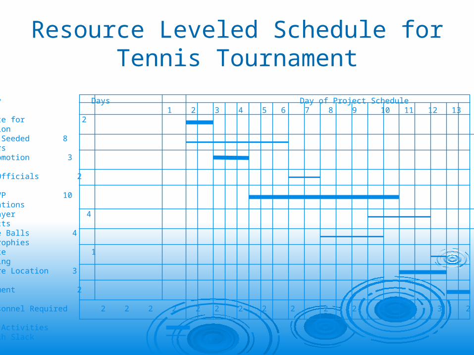
Resource Leveled Schedule for Tennis Tournament

ID Activity Days Day of Project Schedule 1 2 3 4 5 6 7 8 9 10 11 12 13 14 15 16 17 18 19 20A Negotiate for 2 LocationB Contact Seeded 8 PlayersC Plan Promotion 3

D Locate Officials 2

E Send RSVP 10 InvitationsF Sign Player 4 ContractsG Purchase Balls 4 and TrophiesH Negotiate 1 CateringI Prepare Location 3

J Tournament 2

Personnel Required 2 2 2 2 2 2 2 2 2 2 2 2 2 3 2 2 2 2 1 1

Critical Path ActivitiesActivities with Slack

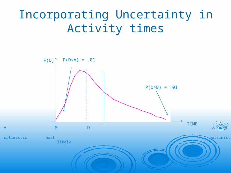
Incorporating Uncertainty in Activity times

A M D B

F(D) P(D<A) = .01

P(D>B) = .01

optimistic most pessimistic likely

TIME

Formulas for Beta Distribution of Activity Duration

Expected Duration

DA M B_

4

6

Variance

VB A

6

2

Note: (B - A )= Range or 6

Activity Means and Variances for Tennis Tournament

Activity A M B D V A 1 2 3 11 .111 B 5 8 11 C 2 3 4 D 1 2 3 E 6 9 18 F 2 4 6 G 1 3 11 H 1 1 1 I 2 2 8 J 2 2 2

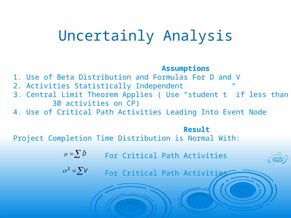
Uncertainly Analysis

Assumptions1. Use of Beta Distribution and Formulas For D and V2. Activities Statistically Independent3. Central Limit Theorem Applies ( Use “student t” if less than 30 activities on CP) 4. Use of Critical Path Activities Leading Into Event Node

ResultProject Completion Time Distribution is Normal With:

For Critical Path Activities

For Critical Path Activities

D_

2 V

Completion Time Distribution for Tennis Tournament

Critical Path Activities D V A 2 4/36 C 3 4/36 E 10 144/36 I 3 36/36 J 2 0

= 20 188/36 = 5.2 = 2

Question

What is the probability of an overrun if a 24 day completion time is promised?

24

P (Time > 24) = .5 - .4599 = .04 or 4%

Days

2 52 .

ZX

Z

Z

24 20

52175

..

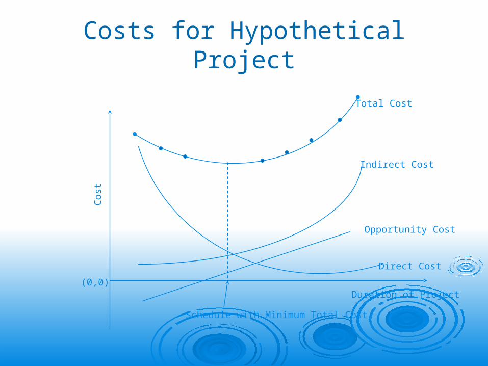
Costs for Hypothetical ProjectC

ost

(0,0)

Schedule with Minimum Total Cost

Duration of Project

Total Cost

Indirect Cost

Opportunity Cost

Direct Cost

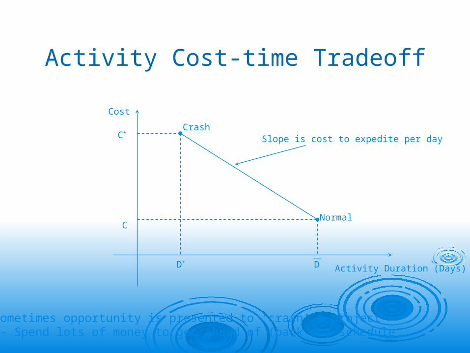
Activity Cost-time Tradeoff

C

C*

D* D Activity Duration (Days)

Normal

CrashSlope is cost to expedite per day

Cost

Sometimes opportunity is presented to ‘crash’ a project - Spend lots of money to get ahead of (back on) schedule

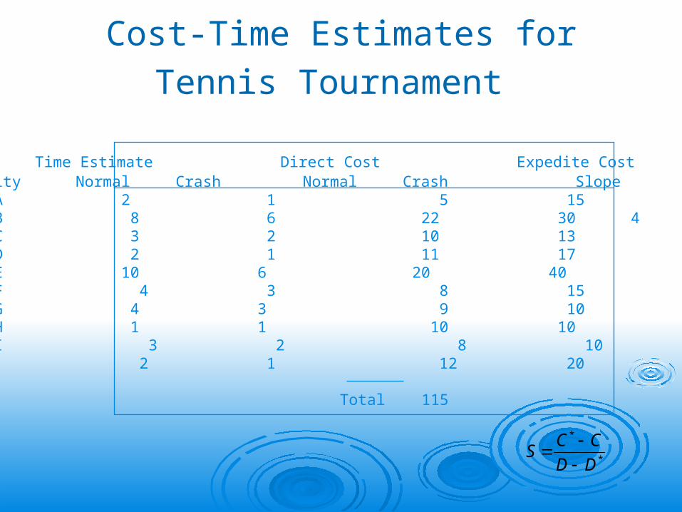
Cost-Time Estimates for Tennis

Tournament

Time Estimate Direct Cost Expedite CostActivity Normal Crash Normal Crash Slope A 2 1 5 15 10 B 8 6 22 30 4 C 3 2 10 13 D 2 1 11 17 E 10 6 20 40 F 4 3 8 15 G 4 3 9 10 H 1 1 10 10 I 3 2 8 10 J 2 1 12 20 Total 115

*

*

DD

CCS

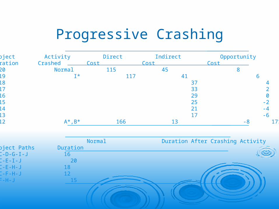
Progressive Crashing

Project Activity Direct Indirect Opportunity TotalDuration Crashed Cost Cost Cost Cost 20 Normal 115 45 8 168 19 I* 117 41 6 164 18 37 4 17 33 2 16 29 0 15 25 -2 14 21 -4 13 17 -6 12 A*,B* 166 13 -8 171

Normal Duration After Crashing ActivityProject Paths DurationA-C-D-G-I-J 16A-C-E-I-J 20A-C-E-H-J 18A-C-F-H-J 12B-F-H-J 15

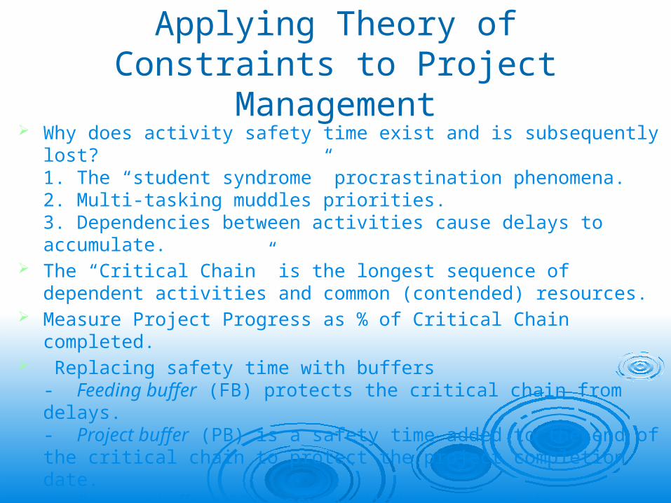
Applying Theory of Constraints to Project Management

Why does activity safety time exist and is subsequently lost?1. The “student syndrome” procrastination phenomena.2. Multi-tasking muddles priorities.3. Dependencies between activities cause delays to accumulate.

The “Critical Chain” is the longest sequence of dependent activities and common (contended) resources.

Measure Project Progress as % of Critical Chain completed. Replacing safety time with buffers

- Feeding buffer (FB) protects the critical chain from delays.- Project buffer (PB) is a safety time added to the end of the critical chain to protect the project completion date.- Resource buffer (RB) ensures that resources (e.g. rental equipment) are available to perform critical chain activities.

Accounting for Resource Contention Using Feeding Buffer

J2

B8

START

A2 C3 D2 G4

E10 I3

F4 H1

FB=7

FB=5

NOTE: E and G cannot be performed simultaneously (same person)

Set feeding buffer (FB) to allow one day total slack

Project duration based on Critical Chain = 24 days

Incorporating Project Buffer

J2

B4

START

A2 C3 D2 G2

E5 I3

F2 H1

FB=2

FB=3

NOTE: Reduce by ½ all activity durations > 3 days to eliminate safety time

Redefine Critical Chain = 17 days

Reset feeding buffer (FB) values

Project buffer (PB) = ½ (Original Critical Chain-Redefined Critical Chain)

PB=4

Sources of Unexpected Problems

Cost Time Performance

Difficulties requiremore resources

Scope of workincreases

Initial bids orestimates were toolow

Reporting was pooror untimely

Budgeting wasinadequate

Corrective controlwas not exercised intime

Price changes ofinputs

Delay owing totechnical difficulties

Initial time estimateswere optimistic

Task sequencingwas incorrect

Required resourcesnot available asneeded

Necessary precedingtasks wereincomplete

Client-generatedchanges

Unforeseengovernmentregulations

Unexpectedtechnical problemsarise

Insufficientresources areavailable

Insurmountabletechnical difficulties

Quality or reliabilityproblems occur

Client requireschanges inspecifications

Complications withfunctional areas

A technologicalbreakthrough occurs