INVESTIGATION AND OPTIMIZATION OF A POROUS SINTERED ...

INVESTIGATION AND OPTIMIZATION OF A POROUS SINTERED

CERAMIC MATERIAL IN A GRINDING APPLICATION

by

Laura Clark

A Thesis

Submitted to the Faculty

of the

WORCESTER POLYTECHNIC INSTITUTE

in partial fulfillment of the requirements for the

Degree of Master of Science

in

Material Science & Engineering

May 2009

APPROVED:

Dr. Diran Apelian, Advisor

Howmet Professor, Director of Metals Processing Institute

Dr. Richard D. Sisson Jr., Head of Department

George F. Fuller Professor, Director of Manufacturing and Materials Engineering

i

Abstract

Porous sintered ceramic foam made of 99.8% Alumina (Al2O3) was investigated for

grinding applications in metallic bearings. The properties of this alumina foam were

investigated and correlated to the grinding performance in an I.D. grinding application.

The mechanical properties, such as density and Young‟s Modulus, were correlated to

grinding performance. The physical properties, investigated with Scanning Electron

Microscope (SEM) analysis and a CT Scan, were used to study sintering behavior and

porosity size and distribution. This work found an optimal friability and sintering

temperature for the alumina foam grinding wheels. This will enable the alumina foam to

become a viable grinding product and compete with the conventional vitrified products.

This would be significant since the alumina foam has mainly one ingredient and is

manufactured with a simpler process. It can also support a higher porosity than

conventional grinding wheels, which has proven to provide better grinding performance

and coolant access, keeping the work piece cooler and avoiding thermal damage.

ii

Acknowledgements

I would like to thank Saint-Gobain for allowing me to conduct my research with them. I

would like to thank my on-site project advisors, Muthu Jeevanantham and Emmanuel

Francois, for their guidance and support. Muthu made this project possible by

coordinating this project with Saint-Gobain and was a key resource. Emmanuel directed

my research and made sure my work was within the guidelines of a thesis.

I would also like to thank Jay Stewart, Steve Fox, and Adam Bujonowski, the Bonded

Research Technicians that helped me run machines and gather data. Also the technicians

and engineers in the Higgins Grinding and Technology Center, Roger Zaleski, Milo

Howard, Greg Lafond, and Kristen Breder who helped conduct the grinding tests.

I would also like to thank Professor Diran Apelian of Worcester Polytechnic Institute,

for being my academic advisor. Professor Apelian helped focus my work to create a

thorough and coherent thesis. He also reviewed my writing and provided constructive

feedback that has improved my thesis and I will keep in mind in future writing.

iii

Table of Contents Table of Figures & Tables .................................................................................................. v

Executive Summary ............................................................................................................ 1

1.0 Introduction ................................................................................................................... 3

2.0 Literature Review.......................................................................................................... 5

2.1 Basics of Grinding ................................................................................................... 5

2.2 Ceramics Used in Grinding ...................................................................................... 5

2.3 Current Limitations .................................................................................................. 6

2.4 Alumina Foam: Fabrication ..................................................................................... 8

2.5 Properties ................................................................................................................. 9

2.6 Current Applications .............................................................................................. 12

2.7 Grinding Performance of Alumina Foam: A Status Report................................... 14

2.8 Summary ................................................................................................................ 16

3.0 Objectives ................................................................................................................... 17

4.0 Procedure .................................................................................................................... 18

4.1 Sample Preparation Phase 1 ................................................................................... 18

4.2 Sample Preparation Phase 2 ................................................................................... 20

4.3 Wheel Fabrication .................................................................................................. 21

4.4 Mechanical Property Evaluation ............................................................................ 23

4.5 Physical Property Evaluation ................................................................................. 26

5.0 Results ......................................................................................................................... 28

5.1 Mechanical Properties - Phase 1 ............................................................................ 28

5.2 Physical Properties - Phase 1 ................................................................................. 34

5.2.1 Scanning Electron Microscope Analysis - Phase 1 ........................................ 34

5.2.2 CT Scan – Phase 1 ......................................................................................... 55

5.3 Grinding Test : Fine Grind – Phase 1 .................................................................... 57

5.3.1 Power (HP/in.) vs. Cumulative MR (in3/in)................................................... 57

5.3.2 Forces: Ft, Fn (lb/in) vs. Cumulative MR (in3/in) ......................................... 59

5.3.3 Surface Roughness: Ra, Rz (µin) vs. Cum. MR (in3/in) ................................ 61

5.3.4 Surface Waviness: Wa, Wt (µin) vs. Cum. MR (in3/in) ................................ 62

5.3.5 Wheel Wear – Phase 1 ................................................................................... 64

iv

5.4 Grinding Test: Rough Grind – Phase 1 .................................................................. 65

5.4.1 Power (HP/in.) vs. Cumulative MR (in3/in) .................................................. 65




5.5 Mechanical Properties – Phase 2 ........................................................................... 67

5.6 Physical Properties – Phase 2 ................................................................................ 69

5.6.1 Scanning Electron Microscope Analysis – Phase 2 ....................................... 69

5.6.2 CT Scan – Phase 2 ......................................................................................... 84

5.7 Grinding Test : Fine Grind – Phase 2 .................................................................... 87

5.7.1 Power (HP/in.) vs. Cumulative MR (in3/in)................................................... 87




5.7.5 Wheel Wear – Phase 2 ................................................................................... 96

6.0 Discussion ................................................................................................................... 98

6.1 Mechanical Properties - Phase 1 ............................................................................ 98

6.2 Physical Properties - Phase 1 ................................................................................. 99

6.3 Grinding Test - Phase 1........................................................................................ 101

6.4 Mechanical Properties - Phase 2 .......................................................................... 102

6.5 Physical Properties - Phase 2 ............................................................................... 103

6.6 Grinding Test – Phase 2 ....................................................................................... 104

7.0 Conclusions ............................................................................................................... 106

8.0 Suggestions for Future Work .................................................................................... 108

Appendix I – Grinding .................................................................................................... 109

Appendix II - Sintering ................................................................................................... 119

Appendix III – Three-point Bend Test Data ................................................................... 132

v

Table of Figures & Tables

Figure 1 : SEM Picture of NorFoam® (150x). [16] ........................................................... 3

Figure 2 : SEM Picture of Current Standard Vitrified Wheel (3000x). [16] ...................... 4

Figure 3: Frictional Components of Grinding. [16] ............................................................ 5

Figure 4: Pre-bonded Clusters of Grain. [17] ..................................................................... 7

Figure 5: SEM Picture of a Vortex Wheel (20x). [16] ....................................................... 7

Figure 6: Alumina Foam Fabrication Process. [16] ............................................................ 8

Figure 7: NorFoam® Properties. [16] ............................................................................... 10

Figure 8: SEM Picture of NorFoam® Structure (150x). [16] ........................................... 10

Figure 9: Interconnected Macropores; Arrows point to Interconnected Pores. [16] ........ 11

Figure 10: Frequency vs. Macropore Length. [16] ........................................................... 11

Figure 11: Permeability of NorFoam®: Pressure Drop vs. Air Flow Rate. [16] .............. 12

Figure 12: NorFoam® compared to current burner block material. [16] ......................... 12

Figure 13: Alumina Foam: EMOD vs. Porosity. [12] ...................................................... 14

Figure 14: Fine Grind: A - Power vs. Cumulative Material Removal; B - Normal Force

vs. Cumulative Material Removal. [12] ............................................................................ 15

Figure 15: Fine Grind: A - Surface Roughness vs. Cumulative Material Removal; B -

Surface Waviness vs. Cumulative Material Removal. [12] .............................................. 15

Figure 16: Rough Grind: A - Unit Power vs. Cumulative Material Removal; B - Normal

Force vs. Cumulative Material Removal. [12].................................................................. 15

Figure 17: Procedure Flowchart........................................................................................ 18

Figure 18: Microstructure Coarsening: Low Initial Packing Density. [9] ........................ 19

Figure 19: Density vs. Time: Wide and Narrow Particle Distribution. [9] ....................... 19

Figure 20: Drill Press…………………………………………………………………….22

Figure 21: Standard Vitrified Wheel. ................................................................................ 21

Figure 22: Alumina Wheels before Grind Test 1: A. CT3000; B. AL260; C. AL261; D.

AL262. .............................................................................................................................. 22

Figure 23: Grinding Test Parameters. ............................................................................... 22

Figure 24: Cellular Solids: A - Two-dimensional honeycomb; B - Three dimensional

foam with open cells. [2] .................................................................................................. 23

Figure 25: Three Point Bend Test and Crush Test Diagram ............................................. 24

Figure 26: Typical Crush Test Data for A - Elastomeric Compression; B - Elastomeric

Tension; C – Plastic Compression; D – Plastic Tension; E – Brittle compression; F –

Brittle Tension. [2] ............................................................................................................ 25

Figure 27: Grindo-Sonic Machine. ................................................................................... 26

Figure 28: Grindo-Sonic sample set-up: A - Probe; B – Striker. ...................................... 26

Figure 29: Scanning Electron Microscope (SEM). ........................................................... 27

Figure 30: Porosity vs. Sample – Phase 1 ......................................................................... 29

Figure 31: EMOD vs. Sample Set Phase 1. ...................................................................... 30

Figure 32: MOR vs. Sample Set – Phase 1. ...................................................................... 31

Figure 33: Young's Modulus vs. Sample from Bar Grindo-sonic Values – Phase 1 ........ 32

Figure 34: Crush Test - Load vs. Time (AL261) – Phase 1. ............................................. 33

Figure 35: Crush Test - Load vs. Time (Initial Section) (AL261) – Phase 1. .................. 33

Figure 36: Crush Test - Stress vs. Strain (AL261) – Phase 1. .......................................... 34

Figure 37: CT3000 (50x) - Macropores ............................................................................ 35

vi

Figure 38: CT 3000 (50x) Interconnected Pores............................................................... 36

Figure 39: CT3000 (100x) Macropore & Interconnected Porosity .................................. 37

Figure 40: CT3000 (500x) Particle Size ........................................................................... 38

Figure 41: AL260 (50x) Macropores. ............................................................................... 39

Figure 42: AL260 (50x) Interconnected Pores. ................................................................ 40

Figure 43: AL260 (1000x) Large Particle. ....................................................................... 41

Figure 44: AL260 (1000x) Particle and Pore Size. ........................................................... 42

Figure 45: AL260 (1000x) Particle Size. .......................................................................... 43




Figure 49: AL261 (1000x) Particle and Innterconnected Pore. ........................................ 47




Figure 53: AL262 (200x) Large Particle in Pore. ............................................................. 51

Figure 54: AL262 (500x) Particle Size at Pore Junction. ................................................. 52

Figure 55: AL262 (500x) Particle Size. ............................................................................ 53

Figure 56: Average Pore Size (µm) vs. Sample – Phase 1. .............................................. 54

Figure 57: Interconnected Pore Size vs. Sample – Phase 1. ............................................. 54

Figure 58: CT Scan – Phase 1 (CT3000 #1). .................................................................... 55

Figure 59: CT Scan – Phase 1 (CT3000 #2) ..................................................................... 56

Figure 60: CT Scan – Phase 1 (CT3000 #3). .................................................................... 57

Figure 61: Phase 1 - Power (Standard #1).........................................................................58

Figure 62: Phase 1: Power (Standard #2)……………………….………...……….…....58

Figure 63: Phase 1 - Power (CT3000 #2)……………………….….……...………...…..58

Figure 64: Phase 1 - Power (CT3000 #3)………………………….………….…...….....58

Figure 65: Phase 1 - Power (AL260#1)………………………………….…………...….58

Figure 66: Phase 1 - Power (AL260#2)……………………………………….………....58

Figure 67: Phase 1 - Power (AL261 #1)…........................................................................59

Figure 68: Phase 1 - Power (AL261 #3)………….. ………………………….……...….59

Figure 69: Phase 1 - Power (AL262 #1)…………………………………………...…….59

Figure 70: Phase 1 - Power (AL262 #2).………………………………………..…….....59

Figure 71: Phase 1 – Forces (Vit. Stand. #1)……………………………………...……..60

Figure 72: Phase 1 - Forces (Vit. Stand. #2)………………………………………...…...59

Figure 73: Phase 1 - Forces (CT3000 #2)……………………………………………......60

Figure 74: Phase 1 - Forces (CT3000 #3)……………………………………………......60

Figure 75: Phase 1 - Forces (AL260 #1)…………………………………………………60

Figure 76: Phase 1 - Forces (AL260 #2)……………………………………………...….60

Figure 77: Phase 1 - Forces (AL261 #1)……………………………………………...….61

Figure 78: Phase 1 - Forces (AL261 #3)………………………………………………....60

Figure 79: Phase 1 - Forces (AL262 #1)…………………………………………………61

Figure 80: Phase 1 - Forces (AL262 #2)………………………………………………....61

Figure 81: Phase 1 - Surface Roughness (Vit. Stand. 1)……………………………...….61

Figure 82: Phase 1 - Surface Roughness (Vit. Stand. 2)…………………………...…….61

vii

Figure 83: Phase 1 - Surface Roughness (CT3000 #2)……………………...…………...62

Figure 84: Phase 1 - Surface Roughness (CT3000 #3)……………………………...…...61

Figure 85: Phase 1 - Surface Roughness (AL260 #1)……………………………………62



Figure 88: Phase 1 - Surface Roughness (AL261 #3)....................................................... 62


Figure 90: Phase 1 - Surface Roughness (AL262 #2)....................................................... 62

Figure 91: Phase 1 - Surface Waviness (Vit. Stand. 1)…………………………………..63

Figure 92: Phase 1 - Surface Waviness (Vit. Stan. 2). ...................................................... 63

Figure 93: Phase - Surface Waviness (CT3000 #2)……………………………………...63

Figure 94: Phase 1 - Surface Waviness (CT3000 #3). ...................................................... 63

Figure 95: Phase 1 - Surface Waviness (AL260 #1)……………………………………..64

Figure 96: Phase 1 - Surface Waviness (AL260 #2)......................................................... 63


Figure 98: Phase 1 - Surface Waviness (AL261 #3)......................................................... 64


Figure 100: Phase 1 - Surface Waviness (AL262 #2). ...................................................... 64

Figure 101: Phase 1 - Rough - Power (Vit. 1)……………………………...……………65

Figure 102: Phase 1 - Rough - Power (Vit. 2). ................................................................. 65

Figure 103: Phase 1 - Rough - Forces (Vit. 1)……………………………...…………....66

Figure 104: Phase 1 - Rough - Forces (Vit. 2). ................................................................. 66

Figure 105: Phase 1 - Rough - Surf. Rough. (Vit. 1)……………………………...……..66

Figure 106: Phase 1 - Rough - Surf. Rough. (Vit. 2). ....................................................... 66

Figure 107: Phase 1 - Rough - Surf. Wav. (Vit. 1)………………………………...…….67

Figure 108: Phase 1 - Rough - Surf. Wav. (Vit. 2). .......................................................... 67

Figure 109: Porosity vs. Sample - Phase 2. ...................................................................... 68

Figure 110: 356A (50x) Macropores. ............................................................................... 69

Figure 111: 356A (50x) Interconnected Pores. ................................................................. 70

Figure 112: 356A (200x) Arrow points to striations. ....................................................... 71

Figure 113: 356A (3000x). ............................................................................................... 72

Figure 114: 356B (50x) Macropores................................................................................. 73

Figure 115: 356B (50x) Interconnected Pores. ................................................................. 74

Figure 116: 356B (100x) Large Particle. .......................................................................... 75

Figure 117: 356B (3000x). ................................................................................................ 76

Figure 118: 356C (50x) Macropores................................................................................. 77

Figure 119: 356C (50x) Interconnected Pores. ................................................................. 78

Figure 120: 356C (100x). .................................................................................................. 79

Figure 121: 356C (3000x). ................................................................................................ 80

Figure 122: 356D (50x) Macropores. ............................................................................... 81

Figure 123: 356D (50x) Interconnected Pores. ................................................................. 82

Figure 124: 356D (100x). ................................................................................................. 83

Figure 125: 356D (3000x). ............................................................................................... 84

Figure 126: CT Scan - Phase 2 (356A). ........................................................................... 85

Figure 127: CT Scan - Phase 2 (356B). ............................................................................ 86

Figure 128: CT Scan - Phase 2 (356C). ............................................................................ 86

viii

Figure 129: CT Scan - Phase 2 (356D). ........................................................................... 87

Figure 130: Phase 2 - (356A #1)…………………………………………………………88

Figure 131: Phase 2 - Power (356A #2)............................................................................ 88

Figure 132: Phase 2 - Power (356A #3)............................................................................ 88

Figure 133: Phase 2 - Power (356B #1)………………………………………………….88

Figure 134: Phase 2 - Power (356B #2). ........................................................................... 88

Figure 135: Phase 2 - Power (356B #3). ........................................................................... 88

Figure 136: Phase 2 - Power (356C #1)………………………………………………….88

Figure 137: Phase 2 - Power (356C #2). ........................................................................... 89

Figure 138: Phase 2 - Power (356C #3). ........................................................................... 89

Figure 139: Phase 2 - Power (356D #1)………………………………………………….89

Figure 140: Phase 2 - Power (356D #2)............................................................................ 89

Figure 141: Phase 2 - Power (356D #3)............................................................................ 89

Figure 142: Phase 2 - Forces (356A #1)……………………………………..…..…....…90

Figure 143: Phase 2 - Forces (356A #2). .......................................................................... 90

Figure 144: Phase 2 - Forces (356A #3). .......................................................................... 90

Figure 145: Phase 2 - Forces (356B #1)………………………………………...….........90

Figure 146: Phase 2 - Forces (356B #2). .......................................................................... 90

Figure 147: Phase 2 - Forces (356B #3). .......................................................................... 91

Figure 148: Phase 2 - Forces (356C #1)…………………………………………… ….91

Figure 149: Phase 2 - Forces (356C #2). .......................................................................... 91

Figure 150: Phase 2 - Forces (356C #3). .......................................................................... 91

Figure 151: Phase 2 - Forces (356D #1)……………………… ………………….……91

Figure 152: Phase 2 - Forces (356D #2). .......................................................................... 91

Figure 153: Phase 2 - Forces (356D #3). .......................................................................... 92

Figure 154: Phase 2 - Surface Roughness (356A #1)……………………………...…….92

Figure 155: Phase 2 - Surface Roughness (356A #2). ...................................................... 92

Figure 156: Phase 2 - Surface Roughness (356A #3). ...................................................... 92

Figure 157: Phase 2 - Surface Roughness (356B #1)…………………………………....93

Figure 158: Phase 2 - Surface Roughness (356B #2). ...................................................... 93

Figure 159: Phase 2 - Surface Roughness (356B #3). ...................................................... 93

Figure 160: Phase 2 - Surface Roughness (356C #1)………………………………........93

Figure 161: Phase 2 - Surface Roughness (356C #2). ...................................................... 93

Figure 162: Phase 2 - Surface Roughness (356C #3). ...................................................... 93

Figure 163: Phase 2 - Surface Roughness (356D #1)…………………………...…….…94

Figure 164: Phase 2 - Surface Roughness (356D #2). ...................................................... 94

Figure 165: Phase 2 - Surface Roughness (356D #3). ...................................................... 94

Figure 166: Phase 2 - Surface Waviness (356A #1)……………………………………..94

Figure 167: Phase 2 - Surface Waviness (356A #2). ........................................................ 94

Figure 168: Phase 2 - Surface Waviness (356A #3). ........................................................ 95

Figure 169: Phase 2 - Surface Waviness (356B #1)………………...……………...……95

Figure 170: Phase 2 - Surface Waviness (356B #2). ........................................................ 95

Figure 171: Phase 2 - Surface Waviness (356B #3). ........................................................ 95

Figure 172: Phase 2 - Surface Waviness (356C #1)………………………………...…...95

Figure 173: Phase 2 - Surface Waviness (356C #2). ........................................................ 95

Figure 174: Phase 2 - Surface Waviness (356C #3). ........................................................ 96

ix

Figure 175: Phase 2 - Surface Waviness (356D #1)……………………………………..96

Figure 176: Phase 2 - Surface Waviness (356D #2). ........................................................ 96

Figure 177: Phase 2 - Surface Waviness (356D #3). ........................................................ 96

Figure 178: Sintering Stages. [9] .................................................................................... 101

Figure 179: Diagram of Basic Grinding. [4] ................................................................... 109

Figure 180: Wheel Depth of Cut vs. Force Intensity. [4] ............................................... 110

Figure 181: Metal Removal Rate vs. Normal Force. [4] ................................................ 111

Figure 182: Metal Removal Parameter vs. Wheelspeed. [4] .......................................... 112

Figure 183: Diagram of Dressing. [4]…………………………………………………..113

Figure 184: Dressing Examples. [4] ............................................................................... 113

Figure 185: Affects of Dressing on Grinding Performance: Metal Removal Rate vs.

Normal Force. [4]............................................................................................................ 114

Figure 186: Effect of the Effective Diamater on Grinding Performance: Material

Removal Rate v.s Force Intensity. [4] ............................................................................ 115

Figure 187: Surface Finish vs. Force Intensity. [4] ........................................................ 117

Figure 188: Surface Finish vs. Metal Removal Rate. [4] ............................................... 118

Figure 189: Stages of Sintering. [9] ................................................................................ 121

Figure 190: SEM pictures of Necking. [9]...................................................................... 122

Figure 191: Necking Model. [9] ..................................................................................... 123

Figure 192: Surface Defects. [9] ..................................................................................... 124

Figure 193: Grain Boundary. [9] .................................................................................... 124

Figure 194: Diffusion vacancy movement. [9] ............................................................... 125

Figure 195: Pore Coarsening. [9] .................................................................................... 126

Figure 196: Densification in different atmospheres. [9] ................................................. 128

Figure 197: Dihedral Angle. [9]...................................................................................... 128

Figure 198: Grain Boundary Movement. [9] .................................................................. 129

Figure 199: Curved Particle. [9] ..................................................................................... 129

Figure 200: Particles Necking. [8] .................................................................................. 130

Figure 201: Flexure Load vs. Flexure Extension - Three-point bend test (CT3000). .... 132

Figure 202: Flexure Load vs. Flexure Extension - Three-point bend test (AL260). ...... 133

Figure 203: Flexure Load vs. Flexure Extension - Three-point bend test (AL261). ...... 134

Figure 204: Flexure Load vs. Flexure Extension - Three-point bend test

(AL262)………………………………………………………………………………....135

Table 1: Alumina Foam Properties [2] ............................................................................... 9 Table 2: Sample Formulation for Friability. ..................................................................... 19

Table 3: Sample Formulation for Porosity Control. ......................................................... 21 Table 4: CT Scan Parameters. ........................................................................................... 27 Table 5: Density - Phase 1 ................................................................................................ 28

Table 6: Porosity Calculations – Phase 1 .......................................................................... 29 Table 7: Three-point Bent Test Phase 1 ............................................................................ 30 Table 8: Wheel Grindo-sonic Values – Phase 1 ............................................................... 31 Table 9: Bar Grindo-sonic Values - Phase 1 ..................................................................... 32 Table 10: Pore Size Range from CT Scan – Phase 1 ........................................................ 55 Table 11: Wheel Wear – Phase 1 ...................................................................................... 65

x

Table 12: Mechanical Properties – Phase 2 ...................................................................... 67

Table 13: Calulated Porosity – Phase 2 ............................................................................ 68 Table 14: Pore Size Range from CT Scan - Phase 2........................................................ 84 Table 15: Wheel Wear – Phase 2 ...................................................................................... 97

Table 16: Sintering Processing Effects. [9] .................................................................... 120 Table 17: Geometric Stages of Sintering. [9] ................................................................. 121 Table 18: Data from Three-point bend test (CT3000). ................................................... 132 Table 19: Data from Three-point bend test (AL260). ..................................................... 133 Table 20: Data from Three-point bend test (AL261). ..................................................... 134

Table 21: Data from Three-point bend test (AL262). ..................................................... 135

1

Executive Summary

Conventional grinding wheels are limited to the amount of porosity they can contain,

which is typically less than 40%. High porosity, over 60%, is desired since it is shown

that a higher porosity can increase the Material Removal Rate (MRR), making the wheel

more efficient. Porosity also increases the permeability of a wheel and provides pockets

for coolant, which will provide more effective cooling of the work piece. If the work

piece is sufficiently cooled then thermal damage of the work piece can be avoided.

Conventional wheels typically consist of abrasive in a bond matrix. However, the bond

does not provide any cutting action, and increased friction, power and temperature during

grinding. A grinding wheel that is 100% abrasive is desired to eliminate the negative

effects of the bond. The abrasive must have a structure that is strong enough to perform

well in a grinding application.

A material that can satisfy the need for a high porosity, 100% abrasive grinding wheel is

NorFoam®, which was developed by Saint-Gobain High Performance Materials (HPM)

at the location in Cree, France. NorFoam® is a ceramic foam made from 1µm alumina

particles, with a density of 0.7g/cc and approximately 83% porosity. This material is

currently available for kiln applications, however this work investigates alterations to

NorFoam® to make it suitable for a grinding application.

From research it was found that a first attempt to alter NorFoam® was made. This was

done by changing the density of the foam to 1.0g/cc with 50% 1µm particles and 50%

tabular alumina. Grinding tests showed that this sample was too hard, or not friable

enough, to perform well in an Inner Diameter (I.D.) grinding application. Based on this

knowledge, a study in friability was conducted.

In phase one of this research the focus was altering the friability of the foam. This was

done by varying the particle size of the foam, with 50% 1µm and 50% 1, 20, 50, or

100µm particles. The mechanical and physical properties of these samples were

investigated and a grinding test was conducted to evaluate the grinding performance. An

optimal friability, or particle size, was chosen based on the results. However, the results

also showed variability in regards to grinding performance, which was due to a variation

in porosity throughout the samples.

An effort to control the porosity was the goal of phase two of this research. This was

done by varying the sintering temperature and studying the effects on the properties and

performance. Based on these results, an optimal sintering temperature was found which

produced the least amount of variance in the performance of the samples, particularly in

regards to surface finish which is very important in I.D. grinding.

2

The research done in this paper could lead to the production of a new type of grinding

wheel, which is highly porous and made of only abrasive. This could provide a

breakthrough in the I.D. grinding application and create a new market for Saint Gobain.

This product would also have a simpler and cleaner manufacturing process than the

current standard. This work could also be expanded to other grinding applications, such

as super-finishing.

Super-finishing is a process that removes an outer layer of metal that has been affected by

high temperatures and pressures. This process requires low material removal, which is

where the alumina foam has excelled. The foam would need little to no alteration in

order to begin testing in this application.

In regards to future work with alumina foam in an I.D. application, there are a few

suggestions. A friability between the samples found in research and the optimum

friability found in phase 1 of this study, sintered at the optimum sintering temperature

found in phase 2, should be tested to see if this formulation will outperform the current

standard products. Also, a study in the addition of secondary particles, such as ZrO2,

MgO, and TiO2, should be conducted to see if the particles would improve the grinding

performance of the foam. Finally, a study on the density of the alumina foam should be

conducted. The higher the density, the lower the porosity, and an optimal porosity has

not yet been found.

3

1.0 Introduction

Conventional grinding wheels consist of abrasive media, such as Alumina, Silicon

Carbide, Diamond, Cubic Boron Nitride, and a gluing agent. The „gluing agent‟, or bond,

could be an organic resin or glass. The role of the „gluing agent‟ is to hold the abrasive

particles in a matrix to form a grinding wheel. The „gluing agent‟ does not do any metal

removal, only the abrasive particles. In many conditions, the „gluing agent‟ interferes

with grinding operation and results in increase in friction, power, and temperature during

grinding. Also, conventional grinding wheels are limited to the amount of porosity they

can contain, which is typically less than 40%, as seen in Figure 2. High porosity, over

60%, is desired since it is shown that a higher porosity can increase the Material Removal

Rate (MRR). Porosity also increases the permeability of a wheel and provides pockets

for coolant, which will provide more efficient cooling of the work piece. An alternative

to the conventional grinding wheel is to use a product that does not have any gluing agent

to eliminate limitations due to the „gluing agent‟. In this respect, NorFoam®, was

developed by Saint-Gobain High Performance Materials (HPM) at the location in Cree,

France.

NorFoam® is fabricated without the use of pore formers or an underlying reticulated

structure upon which ceramic slurry is formed. A mixture of abrasive particles in a

slurry, at least one gelling agent, and at least one foaming agent is formed. Foaming

introduces a large number of bubbles within the mixture, which will later form the

porosity within the final foamed abrasive. After gellation, the mixture is dried and fired

such that a foamed abrasive is obtained. Typically, the firing process includes sintering

of the abrasive grains to bond them to each other at temperatures in excess of 1000ºC and

within a range between about 1400ºC to about 2300ºC. [1]

The finished NorFoam® is a light material, with a density of 0.7 g/cc3 and approximately

83% porosity. The particle size is 1μm, and the pores may have an average size of at

least about 1 micron, and vary in size over a large range between about 10 microns and

about 2000 microns.

Figure 1 : SEM Picture of NorFoam® (150x). [1]

4

Figure 2 : SEM Picture of Current Standard Vitrified Wheel (3000x). [1]

This NorFoam® product is currently available for kiln applications, such as insulation

linings, corrosion resistant linings, and furniture blocks. NorFoam® showed an

improvement over the current Fiber board products with less shrinkage and deformation

at high temperature. NorFoam® is also easy to machine and can be cut with plaster

board tooling. [1] Another market that the NorFoam® may succeed in would be a

grinding wheel application.

NorFoam® has high porosity and no bond, as seen in Figure 1, which would be

beneficial in a grinding wheel application. The absence of a bond will eliminate the

friction associated with the bond during grinding. The high porosity can improve the

MRR and provide better cooling of the work piece. The NorFoam® product has a

structure that is capable of producing this high porosity. This project will focus on

creating an alumina foam product based on the current NorFoam® product that would be

suitable for this application. The properties of this foam and how they affect grinding

performance will be investigated. The friability of the NorFoam® will be tailored for an

Inner Diameter grinding application for bearings. Also, methods to control the porosity

of the foam will be studied to create a dependable product.

5

2.0 Literature Review

2.1 Basics of Grinding

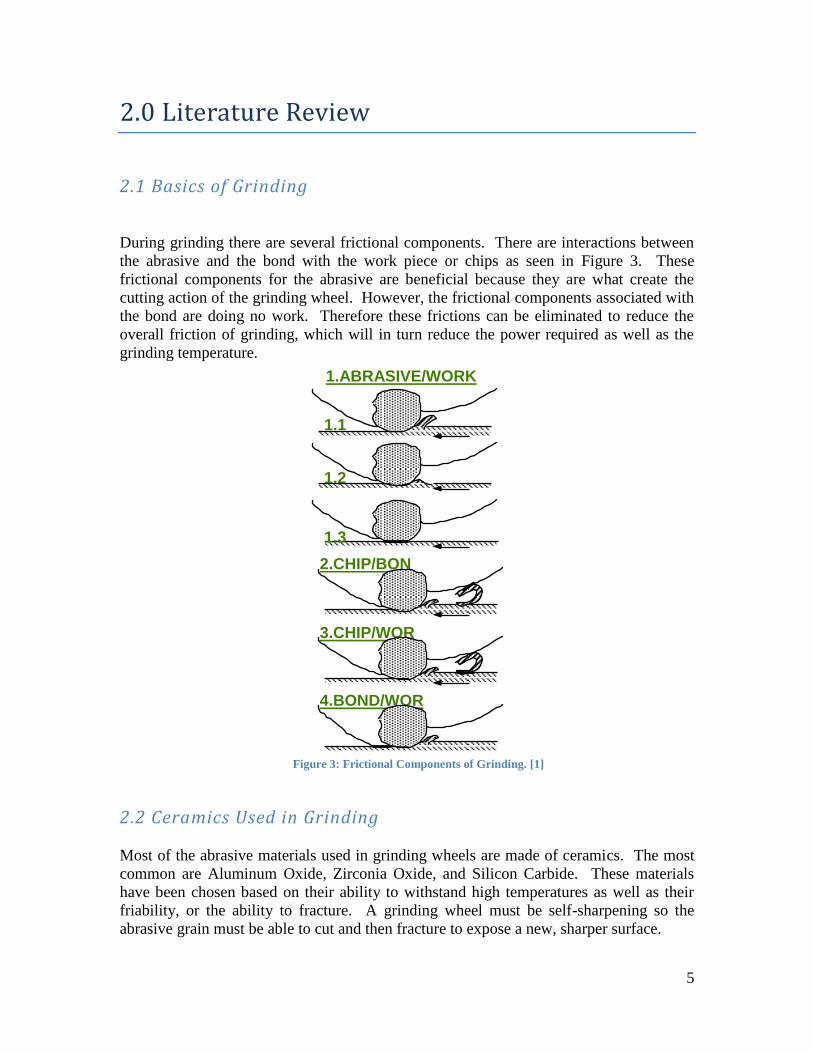
During grinding there are several frictional components. There are interactions between

the abrasive and the bond with the work piece or chips as seen in Figure 3. These

frictional components for the abrasive are beneficial because they are what create the

cutting action of the grinding wheel. However, the frictional components associated with

the bond are doing no work. Therefore these frictions can be eliminated to reduce the

overall friction of grinding, which will in turn reduce the power required as well as the

grinding temperature.

2.2 Ceramics Used in Grinding

Most of the abrasive materials used in grinding wheels are made of ceramics. The most

common are Aluminum Oxide, Zirconia Oxide, and Silicon Carbide. These materials

have been chosen based on their ability to withstand high temperatures as well as their

friability, or the ability to fracture. A grinding wheel must be self-sharpening so the

abrasive grain must be able to cut and then fracture to expose a new, sharper surface.

1.ABRASIVE/WORK

2.CHIP/BOND

3.CHIP/WORK

4.BOND/WORK

1.1

1.2

1.3

Figure 3: Frictional Components of Grinding. [1]

6

These grains must be held together in a matrix to form a grinding wheel; this is done by

adding a bond with the grain. The purpose of the bond is to hold the abrasive grain

during the grinding process, wear at a controlled rate with respect to grain wear, resist

centrifugal forces, and readily expose the grain to the work piece. [2] The five

classifications of bond are vitrified or ceramic, rubber, resinoid, shellac, and organic. [3]

Using one of these five bonds based on the application, wheels are made in varying

amounts of bond, abrasive, and porosity.

The different formulations of grinding wheels are created to have certain properties, such

as hardness and structure. A wheel with high hardness would have a low percentage of

porosity. A wheel with a high or open structure would have a greater percentage of bond

than abrasive. The hardness and the structure of the wheel would affect the friability of

the wheel.

Friability is how easy or difficult it is to break something apart. In the case of a grinding

wheel, there is a certain friability that would allow the wheel to effectively cut a work

piece without significant wear to the grinding wheel. If a wheel is not friable enough,

then the outer layer will not break down and the wheel will become dull. On the other

hand, if a wheel is too friable then the grinding wheel would have significant break down

and would not be able to grind very long, or would have a short life. The friability of a

wheel must be tailored to the desired application to achieve a good grinding performance.

Porosity is another factor that influences grinding performance. “Porosity is typically

present to provide clearance for the chips created during the grinding process, for fluid

transport, and to enhance the various interactions taking place in the grinding zone.” [2]

In order to have good chip clearance, fluid transport and cooling, the porosity must also

be permeable, or have interconnected porosity.

2.3 Current Limitations

There are two common ways of creating high porosity in grinding wheels. First is a

burn-out method where a “pore structure is created by addition of organic pore inducing

media (such as walnut shells) in the wheel mixing stage. These media thermally

decompose upon firing of the green body of abrasive tool, leaving voids or pores in the

cured abrasive tool.” [2] The biggest drawback to this method is the emissions that are

released when the pore inducer is decomposed. Other drawbacks include moisture

absorption in pore inducer, mixing inconsistency, and spring-back after molding.

The second method is the closed cell or bubble method. In this case materials such as

bubble alumina are introduced into the mix which does not need to be burned out. This

eliminates the emissions associated with the first method; however the porosity that is

created is closed porosity, with no interconnected porosity. This means that the wheel

will not be permeable to allow coolant flow and the porosity is typically not large enough

to allow for proper metal chip clearance. [2] The lack of permeability in closed cell

creates higher grinding forces and increased risk of thermal damage. [4] Another method

has been created that is based off the traditional production of grinding wheels, which

7

mixes individual abrasive grains with a bond. This new method takes the grains and

creates pre-bonded clusters of grain, and then bonds the clusters together in the traditional

way to create a grinding wheel with higher porosity. These clusters can be seen in Figure

4.

Figure 4: Pre-bonded Clusters of Grain. [2]

Grinding tests were performed on these wheels, and the results showed a “greater G-ratio,

less chatter, and higher material removal rates, with acceptable surface finish.” [2] This

shows that wheels with a higher porosity have an improved grinding performance.

However, many conventional grinding wheels are unable to achieve high porosity. “Very

porous abrasive composites made with larger grain sizes, higher volume percentages of

grain and softer, organic bond materials have a tendency to slump or stratify during the

intermediate molding and curing stages of manufacturing the grinding tool. For these

reasons, commercially available bonded abrasive tools made with organic bond materials

often are molded to contain no porosity, and typically contain no more than 30 volume%

porosity. They seldom exceed 50 volume% porosity.” [4] A typical structure of a current

grinding wheel can be seen in Figure 5.

Figure 5: SEM Picture of a Vortex Wheel (20x). [1]

8

There is a need to create a grinding product that is able to support high porosity, which

will result in improved grinding performance over the current standard product. The

current burn-out, closed cell, and cluster methods have taken steps towards a higher

porosity grinding wheel. However a larger increase in porosity over the standard that is

interconnected is needed with a method that is simple and has no emissions. One method

that looks promising is an alumina foam, which contains a high amount of porosity that is

interconnected and does not contain any bond. It is created by a simple sintering method

and does not require any organic material to be burned out during the process.

Accordingly, the thesis work focused on studying the key variables in the production of

alumina foam in order to affect grinding performance in respect to the conventional

bonded grinding wheels.

2.4 Alumina Foam: Fabrication

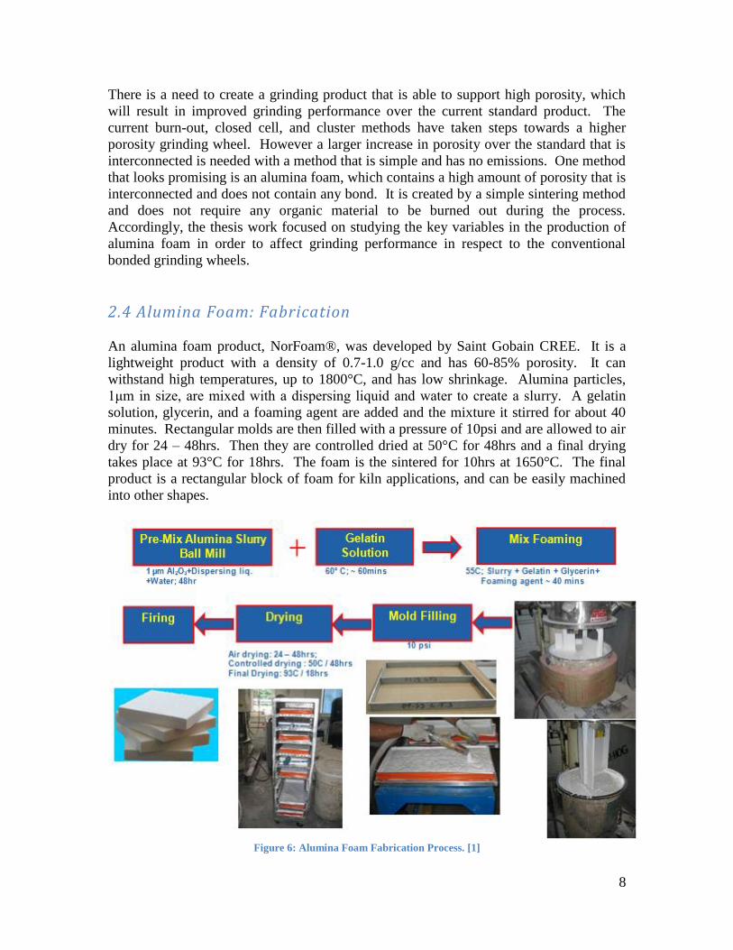
An alumina foam product, NorFoam®, was developed by Saint Gobain CREE. It is a

lightweight product with a density of 0.7-1.0 g/cc and has 60-85% porosity. It can

withstand high temperatures, up to 1800°C, and has low shrinkage. Alumina particles,

1μm in size, are mixed with a dispersing liquid and water to create a slurry. A gelatin

solution, glycerin, and a foaming agent are added and the mixture it stirred for about 40

minutes. Rectangular molds are then filled with a pressure of 10psi and are allowed to air

dry for 24 – 48hrs. Then they are controlled dried at 50°C for 48hrs and a final drying

takes place at 93°C for 18hrs. The foam is the sintered for 10hrs at 1650°C. The final

product is a rectangular block of foam for kiln applications, and can be easily machined

into other shapes.

Figure 6: Alumina Foam Fabrication Process. [1]

9

2.5 Properties

Alumina has some specific properties that make it a successful material in a grinding

application. Alumina has a high Young‟s Modulus and melting temperature, meaning it

will have the ability to grind and withstand the high temperatures associated with

grinding. Other factors that contribute to its success would be its compression strength,

fracture strength, and fracture toughness. These affect the friability of the material, and

show that alumina will resist fracture, but will eventually breakdown as needed in a

grinding application.

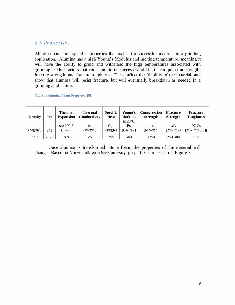
Table 1: Alumina Foam Properties [5]

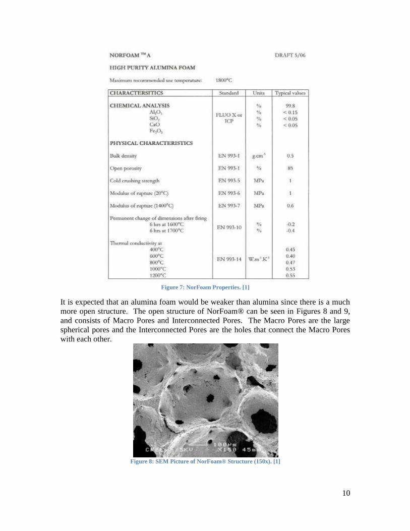
Once alumina is transformed into a foam, the properties of the material will

change. Based on NorFoam® with 85% porosity, properties can be seen in Figure 7.

Density

(Mg/m3)

Tm

(K)

Thermal

Expansion

αsx10^-6

(K^-1)

Thermal

Conductivity

λs

(W/mK)

Specific

Heat

Cps

(J/kgK)

Young's

Modulus

at 20°C

Es

(GN/m2)

Compression

Strength

σcs

(MN/m2)

Fracture

Strength

σfs

(MN/m2)

Fracture

Toughness

K1Cs

(MN/m^(3/2))

3.97 2323 8.8 25 795 380 1750 250-300 3-5

10

Figure 7: NorFoam Properties. [1]

It is expected that an alumina foam would be weaker than alumina since there is a much

more open structure. The open structure of NorFoam® can be seen in Figures 8 and 9,

and consists of Macro Pores and Interconnected Pores. The Macro Pores are the large

spherical pores and the Interconnected Pores are the holes that connect the Macro Pores

with each other.

Figure 8: SEM Picture of NorFoam® Structure (150x). [1]

11

Figure 9: Interconnected Macropores; Arrows point to Interconnected Pores. [1]

Using image analysis, the length and frequency of Macro Pores have been recorded and

is shown in Figure 10. The pores appear to have a wide range of length, typically 150 -

975μm, with the most common lengths being from 150 - 450μm.

Figure 10: Frequency vs. Macropore Length. [1]

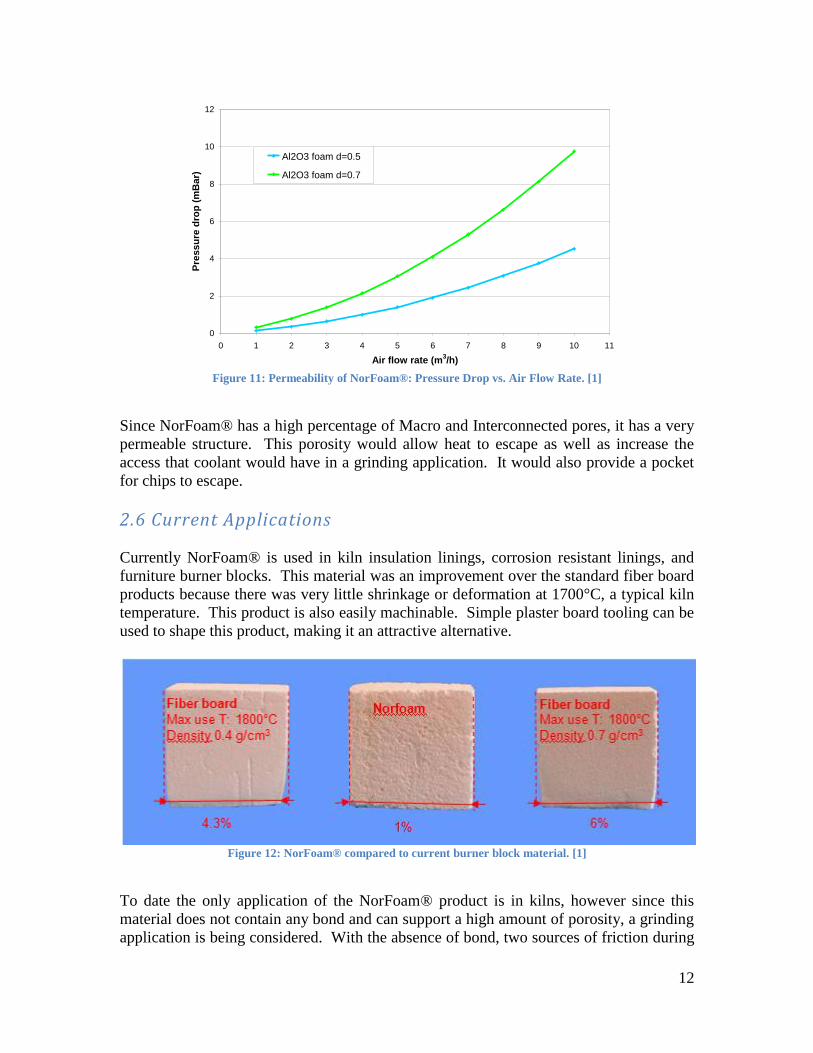
Since Norfoam® has a lot of Interconnected Pores, this increases the permeability of the

foam. Samples of NorFoam® 35x35mm and 12mm thick were tested for their

permeability using air. One sample had a density of 0.5g/cm3 and a second sample had a

density of 0.7g/cm3. As expected, in Figure 11 the foam with the lower density of

0.5g/cm3 had a resulting pressure drop that was lower than the denser sample, showing

that it was more porous or had more interconnected porosity.

0

2

4

6

8

10

12

14

16

18

20

22

24

100 200 300 400 500 600 700 800 900 1000 1100 1200 or more

…

Macropore length (µm)

Fre

qu

en

cy

(%

)

12

Figure 11: Permeability of NorFoam®: Pressure Drop vs. Air Flow Rate. [1]

Since NorFoam® has a high percentage of Macro and Interconnected pores, it has a very

permeable structure. This porosity would allow heat to escape as well as increase the

access that coolant would have in a grinding application. It would also provide a pocket

for chips to escape.

2.6 Current Applications

Currently NorFoam® is used in kiln insulation linings, corrosion resistant linings, and

furniture burner blocks. This material was an improvement over the standard fiber board

products because there was very little shrinkage or deformation at 1700°C, a typical kiln

temperature. This product is also easily machinable. Simple plaster board tooling can be

used to shape this product, making it an attractive alternative.

Figure 12: NorFoam® compared to current burner block material. [1]

To date the only application of the NorFoam® product is in kilns, however since this

material does not contain any bond and can support a high amount of porosity, a grinding

application is being considered. With the absence of bond, two sources of friction during

0

2

4

6

8

10

12

0 1 2 3 4 5 6 7 8 9 10 11

Air flow rate (m3/h)

Pre

ss

ure

dro

p (

mB

ar)

Al2O3 foam d=0.5

Al2O3 foam d=0.7

13

grinding are eliminated between the bond and the work piece, as well as between the chip

and the bond. The high porosity and permeable structure provides better coolant access

and can reduce grinding temperatures. The high porosity can also improve Material

Removal Rate (MRR).

NorFoam® is appealing for a grinding application since it has a high amount of porosity

and no bond. However this is not the first alumina foam product to be invented, nor is it

the first product to deal with these grinding issues. There are many patents that deal with

a similar product.

A patent for a “Ceramic Foam and Method of Preparation” was filed back in 1975 that

focused on creating a filter for molten metals. Alumina was among the ceramics used

and was said to have a controlled permeability and uniformity. This foam was created by

impregnating an organic polymer foam with a refractory, then compressing the foam

through rollers to remove excess refractory. The material is then heated to eliminate the

polymer. The resulting ceramic foam had a permeability ranging from 4,500-5,400 x10-

7cm

2. This foam was said to work very well as a filter, however mentioned issues with

the rolling process. The outer area of the foam became more thinly coated than the inner

area. [6]

Another method describes a “Process of Producing Self-Bonded Ceramic Abrasive

Wheels”. Here it is mentioned that conventional grinding wheels have two firing cycles,

one for the abrasive grits to convert to a crystalline form, and one to develop the bond.

The objective is to eliminate the bond so only one firing cycle is needed. Alumina is hard

and abrasion resistant and is determined as a good candidate and if partially sintered will

have a suitable porosity and structure strength for a grinding tool. Microcrystalline

alumina is used and obtained by the sol-gel process in U.S. patent numbers 4,623,364 and

4,744,802. Other components may be added such as fibrous or particulate ceramics, or

zirconia and metal oxides to serve as toughening agents. The foam is again formed by

infiltrating a foam structure, this time made out of a ceramic, which is coated and heated

to convert alumina to alpha structure and eliminate the pre-form. This method was

chosen since the pre-form can easily escape in the open cell structure, as opposed to using

walnut shells or plastic beads to form the pores. Also, the method of generating foam

with physical or chemical blowing agents was determined too difficult to control. The

resulting wheel was 1.5” in diameter with 42% porosity. It was tested at a speed of

15,700 rpm and had a calculated G-Ratio of 51.3, power draw of 10.1HP/in, and a surface

finish of 41.7μin. [7]

“High Porosity Vitrified Bonded Grinding Wheels” have used similar methods to obtain a

porous structure. A mixture of alumina beads and walnut shells are introduced into the

grinding wheel to get a resulting porosity of 40-70%, with 1-12% of that coming from the

shells and 10-20% coming from the bubble alumina. It was observed that with only

bubble alumina, there were mainly closed pores creating a grinding product that rapidly

deteriorated and porosity that only fluid not chips could enter. Using only the walnut

shells a very open structure was created, however the product did not have the strength

needed for the creep-feed grinding application. Therefore a mixture was used in the

14

wheel, which would possibly be impregnated with a grinding aid after firing, such as

molten sulfur. The resulting wheel was suitable for various steels and metals, and had an

increased wheel life. [8]

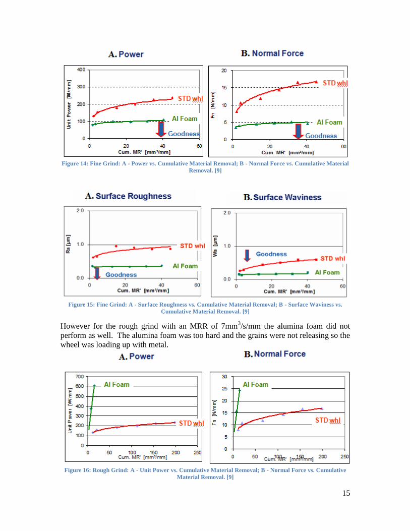
2.7 Grinding Performance of Alumina Foam: A Status Report

Variations of the NorFoam® product have already been created for a grinding

application. In 2006, a foam was made with only CT3000 SG, a density of 0.5g/cm3, and

a firing cycle of 1580°C for 5 hours. This foam was extremely friable, so a new

formulation was created in 2007. This new formulation was a mixture of 50% 1μm

CT3000 SG and 50% tabular alumina with a different diameter. The density was 1g/cm3

and had a firing cycle of 1630°C for 5 hours due to the lower quantity of reactive

alumina. The alumina foam from 2007 showed the following property relationship for

the Young‟s Modulus, or Modulus of Elasticity (EMOD), in Figure 13. [9]

Figure 13: Alumina Foam: EMOD vs. Porosity. [9]

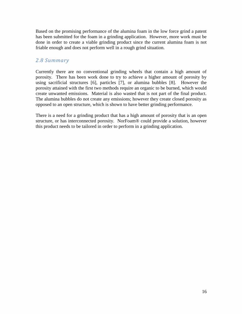
Inner Diameter (I.D.) grinding wheels were cut from the sample and tested in the Higgins

Grinding Technology Center on 5200 steel bearings. For the fine grind with an MRR of

1.5mm3/s/mm the results showed the alumina foam was an improvement over the

standard.

EMOD -Porosity Relationship

0

10

20

30

40

50

60

70

20 30 40 50 60 70 80

Vol% Porosity

EM

OD

(G

Pa)

Al FoamSTD Vitrified

Products

15

Figure 14: Fine Grind: A - Power vs. Cumulative Material Removal; B - Normal Force vs. Cumulative Material

Removal. [9]

Figure 15: Fine Grind: A - Surface Roughness vs. Cumulative Material Removal; B - Surface Waviness vs.

Cumulative Material Removal. [9]

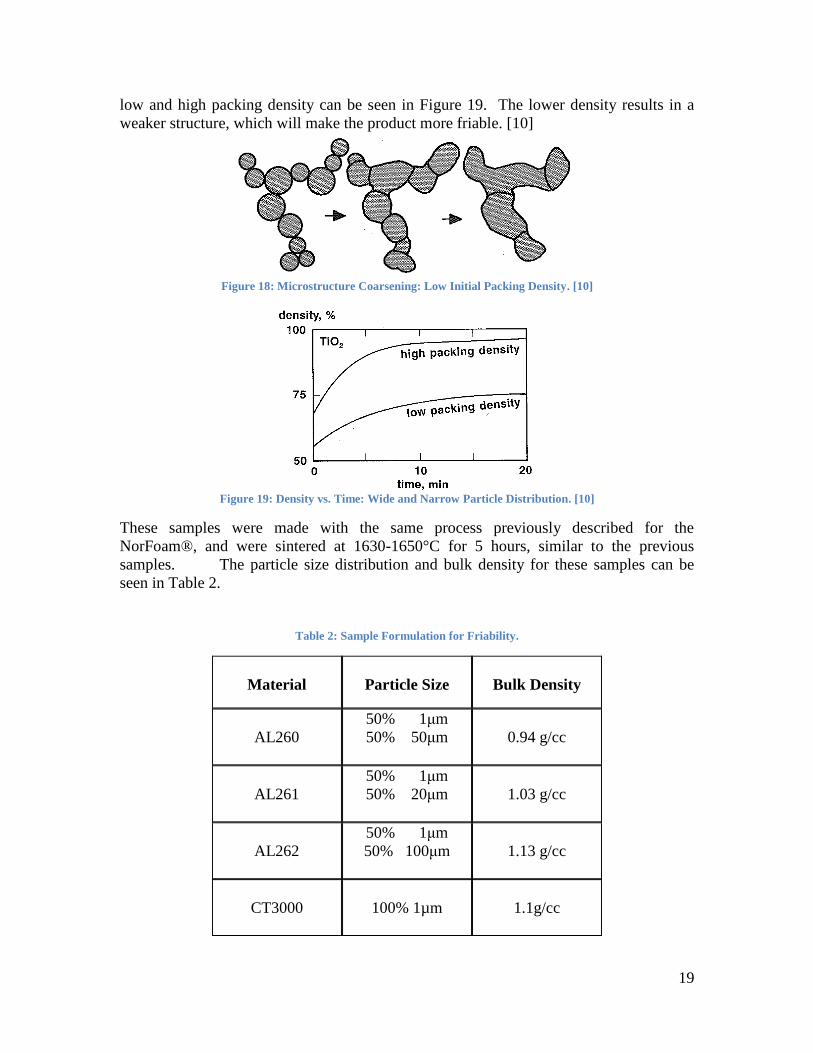
However for the rough grind with an MRR of 7mm3/s/mm the alumina foam did not

perform as well. The alumina foam was too hard and the grains were not releasing so the

wheel was loading up with metal.

Figure 16: Rough Grind: A - Unit Power vs. Cumulative Material Removal; B - Normal Force vs. Cumulative

Material Removal. [9]

16

Based on the promising performance of the alumina foam in the low force grind a patent

has been submitted for the foam in a grinding application. However, more work must be

done in order to create a viable grinding product since the current alumina foam is not

friable enough and does not perform well in a rough grind situation.

2.8 Summary

Currently there are no conventional grinding wheels that contain a high amount of

porosity. There has been work done to try to achieve a higher amount of porosity by

using sacrificial structures [6], particles [7], or alumina bubbles [8]. However the

porosity attained with the first two methods require an organic to be burned, which would

create unwanted emissions. Material is also wasted that is not part of the final product.

The alumina bubbles do not create any emissions; however they create closed porosity as

opposed to an open structure, which is shown to have better grinding performance.

There is a need for a grinding product that has a high amount of porosity that is an open

structure, or has interconnected porosity. NorFoam® could provide a solution, however

this product needs to be tailored in order to perform in a grinding application.

17

3.0 Objectives

The objectives of the thesis are:

Quantify properties of Alumina Foam

Create a friability which is suitable for I.D. grinding

Control porosity to create a dependable product

In terms of the approach followed to meet these objectives, three key steps were taken.

They are summarized below and discussed in greater detail in the procedure and results

sections, respectively.

The first step to creating an alumina foam product is to quantify the properties of alumina

foam. This is a very different product than the standard grinding wheel and alumina

foam‟s mechanical properties need to be correlated to its performance. From this we can

evaluate any trends that occur and compare with behavior of current standard products.

Alumina foam may exhibit different behaviors than current products, or may follow the

same trends.

The next step would be to create a friability that would be suitable for I.D. grinding.

Based on the preliminary tests done with alumina foam it can be seen that the current

friability of the foam had a good grinding performance in the fine grind, or low MRR

test. However the foam did not perform well in the rough grind, or high MRR test. This

was because the wheel did not break down and loaded up with metal, meaning that the

friability was too low for the rough grind situation. A balance between a good friability

for the fine grind and rough grind must be found in order to create a viable grinding

product for I.D. grinding. Based on the conclusion that the current friability is too low

for the rough grind, the friability of the foam must be increased.

Another factor that needs to be taken into consideration is the porosity in the alumina

foam. Currently the porosity size and distribution are not controlled when alumina foam

is manufactured. This is acceptable for the current NorFoam® application where only

the amount of porosity is the concern, however in a grinding application the size and

distribution of porosity can affect the grinding performance. A grinding product must

have repeatable results, so each wheel made should have the same porosity size and

distribution. Efforts must be made to control the porosity; otherwise it would not be

possible to create a dependable grinding product.

18

4.0 Procedure

The procedure includes two different phases of sample preparation, wheel fabrication,

and the evaluation of the mechanical and physical properties. The first sample phase

focused on altering the friability of the foam with various particle size distributions. The

samples were evaluated with mechanical and physical property testing, as well as a

grinding test. From this evaluation an optimal distribution was chosen. Using this

optimal distribution, the second phase of samples focused on controlling the size and

distribution of porosity in the foam by varying the sintering temperature. These samples

were then evaluated using the same methods used for the first phase of samples.

Figure 17: Procedure Flowchart

4.1 Sample Preparation Phase 1

Literature and previous work have established clear that a more friable wheel is needed in

order to perform well in the rough grind cycle. The original alumina foam formulation

contained 50% CT3000 SG 1µm and 50% tabular alumina. To increase the friability of

the material, the tabular alumina was eliminated and replaced with different particle sizes

of CT3000 SG. A distribution of particle sizes will affect the packing density, creating a

lower packing density than the previous samples with a single particle size. This low

packing density will affect the microstructure, and cause grain growth without

densification, as shown in Figure 18. This will result in a lower density after sintering

since the pores are not shrinking. A comparison of the density % with time between a

19

low and high packing density can be seen in Figure 19. The lower density results in a

weaker structure, which will make the product more friable. [10]

Figure 18: Microstructure Coarsening: Low Initial Packing Density. [10]

Figure 19: Density vs. Time: Wide and Narrow Particle Distribution. [10]

These samples were made with the same process previously described for the

NorFoam®, and were sintered at 1630-1650°C for 5 hours, similar to the previous

samples. The particle size distribution and bulk density for these samples can be

seen in Table 2.

Table 2: Sample Formulation for Friability.

Material

Particle Size

Bulk Density

AL260

50% 1μm

50% 50μm

0.94 g/cc

AL261

50% 1μm

50% 20μm

1.03 g/cc

AL262

50% 1μm

50% 100μm

1.13 g/cc

CT3000

100% 1µm

1.1g/cc

20

4.2 Sample Preparation Phase 2

In order to control the porosity throughout the alumina foam, several solutions were

considered. Previous methods that have been used to control porosity in Al2O3 include

chemical control, sacrificial structures, polystyrene beads, and a two-step sintering

process.

The process that used chemical control used carboxylate-alumoxane nanoparticles to

control porosity. These particles contain an alumina core and are surrounded by

carboxylate ligands. The particles can be made from the reaction of boehmite

[Al(O)(OH)]n with a carboxylic acid (HO2CR). Although this process seems to create a

uniform porosity throughout the structure, this process is used commonly for thin films

and would not be applicable for a grinding application. [11]

A sacrificial structure made of an open-cell polymeric structure could be used. This has

been previously used to create SiC based foams, and could possibly be used for an

alumina foam. However, this requires the destruction of a material and could create

emissions. A cleaner process is desired for the alumina foam. [12]

Polystyrene beads have been added to an alumina powder to control the porosity size.

Beads ranging from 1.4 – 2.8mm were added to 0.36µm alumina particles, which had

been modified with 0.5 wt% MgO. These were compacted and heated to 500°C at 1°/min

to remove the organics, and then sintered at 1550°C for 2hr to get a porous ceramic. This

process produced a very controlled porous structure with interconnected porosity,

however this process also requires an organic to be destroyed, so another process is

considered. [13]

A two-step sintering process was developed in an effort to control porosity of sintered

alumina. This process had a precoarsening step where the material was heated at

10°C/min to 800°C for 50hr, and then heated at 4°C/min to 1450°C for sintering. This

study found a larger average pore size with a narrower distribution in pore size. The

amount of closed porosity was lower, meaning that there was a lot of interconnected

porosity. [14]

The two-step sintering process is the most promising for an alumina foam grinding

application. This process led to a study of the effect of the sintering temperature on the

alumina foam. Various sintering temperatures were chosen to study the effect on the

porosity size and distribution. The samples created had the following sintering

temperatures and bulk density as shown in Table 3:

21

Table 3: Sample Formulation for Porosity Control.

Sample

Composition Sintering

Temperature

Bulk Density (g/cc)

356 A 100% 1µm 1700°C/3092°F 1.54

356 B 100% 1µm 1680°C/3056°F 1.55

356 C 100% 1µm 1630°C/2966°F 1.50

356 C 100% 1µm 1590°C/2894°F 1.46

From each of these samples four wheels were made using the same process as described

for the previous set of samples. One of the four wheels was looked at with the CT Scan,

and three of the four went to the HGTC to be tested with the same grinding parameters as

the previous samples. The mechanical and physical properties were investigated using

the same methods as before.

4.3 Wheel Fabrication

Once the alumina foam material has been made, wheels must be cut for I.D. grinding

tests. To make the wheels, a drill press is used with a 15/16” diameter diamond hole saw.

The alumina foam is placed in a container filled with water for better cutting and then

cylinders are cored out from the alumina foam material. Since the material was placed in

water, the cylinders are then dried in an oven at 100°C overnight. Once the cylinders are

dry, they are taken to a machine that is able to drill the I.D. of the wheel to 0.380” and

have the diameter turned down to 1.2”. However, since some of the samples were very

friable, the diameter had to be turned down to 1”. Once the wheels are cut to the correct

specifications, then the samples O.D., I.D., thickness, and weight must be measured.

Figure 20: Drill Press. Figure 21: Standard Vitrified Wheel.

22

Figure 22: Alumina Wheels before Grind Test 1: A. CT3000; B. AL260; C. AL261; D. AL262.

Once the wheels were made, they were sent to the Higgins Grinding Technology Center

(HGTC). There they were tested in an I.D. plunge grind test with the parameters shown

in Figure 23.

Figure 23: Grinding Test Parameters.

Each wheel was initially dressed, and then did five grinds on a part for four sets, or 20

grinds total, unless the wheels loaded up before the 20 grinds. The wheels were not

dressed in between each part, but were dressed in between the fine and rough MRR. Two

23

wheels from each specification were tested along with two standard vitrified wheels with

specification of DG100 428.

4.4 Mechanical Property Evaluation

Once the new alumina foam samples were created, the mechanical properties of the foam

must be investigated. These properties include density, Young‟s Modulus and Modulus

of Rupture.

The density of the foam can be found by measuring the dimensions of a sample and

calculating the volume. Then the weight of the sample is found by placing the sample on

a balance. The density is then calculated by dividing the mass by the volume.

The Young‟s Modulus and Modulus of Rupture affect the stiffness and the wear

resistance of the wheel. These values can be found using a few different tests.

The usual test used to determine the Young‟s Modulus and Modulus of Rupture for

conventional grinding wheels is a three point bend test. This test is performed with an

Instron on samples that are ½in.x 1in.x 4in. in dimension. The load in the Instron was

8kN. The set up can be seen in Figure 25. The modulus values are calculated by the

computer program Bluehill.

Another test that is more common for foams, or cellular solids, is a crush test. The

structure of a cellular solid is shown in Figure 24. The three dimensional foam shown

with open cells closely resembles the structure of alumina foam. Since the structure is

similar, the crush test could provide good results.

Figure 24: Cellular Solids: A - Two-dimensional honeycomb; B - Three dimensional foam with open cells. [5]

The crush test is more commonly used for a foam since a three point bend test could

fracture a layer of the foam and not the entire sample. A crush test will fracture all the

layers of the foam since it compressed the foam until it is flattened. This test can be

performed on the same Instron machine, however different fixturing is used. A large,

flat, circular plunger is used as well as a leveler, which will keep the flat and the force

applied evenly distributed if the sample is slightly uneven. The sample size for this test is

½ in. x ½ in. x ½ in. in dimension. This test also used the 8kN force. A diagram of this

24

procedure can be seen in Figure 25. The output of the test is load vs. time data, which

has an initial fracture line, then multiple fracture points that level off, and then the load

grows exponentially toward the end of the test. The initial fracture line must be isolated

from the rest of the data, converted to Stress vs. Strain, and then the slope of the line is

calculated and is taken as the Young‟s Modulus. Typical data collected with this test can

be seen in Figure 26. It would be expected that the alumina foam would resemble the

data shown for brittle compression.

3 Point Bend Test Crush Test

OLD NEW

sample sample Leveler

Sample size: ½” x ½” x ½” Sample size: ½” x 1” x 4”

LOAD

Figure 25: Three Point Bend Test and Crush Test Diagram

25

Figure 26: Typical Crush Test Data for A - Elastomeric Compression; B - Elastomeric Tension; C – Plastic

Compression; D – Plastic Tension; E – Brittle compression; F – Brittle Tension. [5]

Another way to find the Young‟s Modulus would be to use a Grindo-Sonic Machine.

This machine uses sound waves to calculate a value that can be used in equations to

calculate the Young‟s Modulus. Bars of dimension 1 x ½ x 4in. were used, and three

bars from each specification were tested. The samples were placed on a wooden

apparatus that supported the sample in two places. This is used so that the waves being

measured are not disturbed. The probe from the Grindo-Sonic is placed on the end of the

bar, and the bar is struck on a surface 90° from the probe. The bar is lightly struck until

the same value is obtained three times, and that value is recorded as the Grindo-Sonic

number for that sample.

26

Figure 27: Grindo-Sonic Machine.

Figure 28: Grindo-Sonic sample set-up: A - Probe; B – Striker.

4.5 Physical Property Evaluation

To analyze the physical properties of the alumina foam pictures were taken with a

Scanning Electron Microscope (SEM) as well as X-ray tomography, or a CT Scan. This

analysis is helpful in looking at the sintering behavior, as well as the porosity size and

distribution throughout the sample.

Pictures were taken with an SEM at various magnifications, ranging from 20x – 3000x,

with a 20kV current. The alumina foam samples were first sputter coated with Gold-

Palladium for 90 seconds in order to get a better resolution. These pictures were

analyzed with Orion software, which allowed distances on the picture to be measured.

The size of the grains, the large pores, and the interconnected porosity were measured

using this software.

27

Figure 29: Scanning Electron Microscope (SEM).

The CT Scan was done on wheels that had not been ground with to see the size and

distribution of the pores. This was done using a Phoenix CT Scanner and was run at the

following parameters in Table 4:

Table 4: CT Scan Parameters.

The pore size is recorded and a pore size range is generated. The sample is scanned from

various sections and views to get a good understanding of the porosity throughout the

sample.

28

5.0 Results

The results are presented in the sequence of phase 1 then phase 2. This means that all of

the results for phase 1, including mechanical and physical properties and the grinding

test, will be presented. Then all of the results for phase 2 will be presented in the same

manner.

5.1 Mechanical Properties - Phase 1

Each wheel was measured and weighed before it went through the grinding test. The data

recorded is in Table 5.

Table 5: Density - Phase 1

Sample

O.D.

(in.)

Thickness

(in.)

Hole

(in.)

Weight

(g)

Density

(g/cc)

Bulk

Density

(g/cc)

CT 3000 - 1 1.030 0.942 0.380 11.59 1.04 1.1

CT 3000 - 2 1.030 0.935 0.381 11.48 1.04 1.1

CT 3000 - 3 1.050 0.939 0.376 10.07 0.87 1.1

AVE 0.98

STDEV 0.08

AL 260 - 1 1.030 0.935 0.380 11.54 1.05 0.94

AL 260 - 2 1.050 0.940 0.378 9.94 0.86 0.94

AVE 0.95

STDEV 0.13

AL 261 - 1 1.040 0.935 0.378 10.27 0.91 1.03

AL 261 - 2 1.030 0.936 0.378 10.30 0.93 1.03

AL 261 - 3 1.040 0.935 0.378 10.60 0.94 1.03

AVE 0.93

STDEV 0.02

AL 262 - 1 0.990 0.913 0.388 10.77 1.10 1.13

AL 262 - 2 0.990 0.915 0.388 10.80 1.11 1.13

AL 262 - 3 0.990 0.915 0.385 11.23 1.15 1.13

AVE 1.12

STDEV 0.02

29

From the measured density the percentage of porosity in the wheel can be calculated

using the known density of alumina of 3.97g/cc.

Table 6: Porosity Calculations – Phase 1

Spec

Measured

Density

(g/cc)

Porosity

(%)

CT3000 #1 1.04 74

CT3000 #2 1.04 74

CT3000 #3 0.87 78

AVE 75

STDEV 2.5

AL260 #1 1.05 74

AL260 #2 0.86 78

AVE 76

STDEV 3.4

AL261 #1 0.91 77

AL261 #2 0.93 77

AL261 #3 0.94 76

AVE 77

STDEV 0.4

AL262 #1 1.10 72

AL262 #2 1.11 72

AL262 #3 1.15 71

AVE 72

STDEV 0.7

Figure 30: Porosity vs. Sample – Phase 1

66

68

70

72

74

76

78

80

82

CT3000 AL261 AL260 AL262

Po

rosit

y (

%)

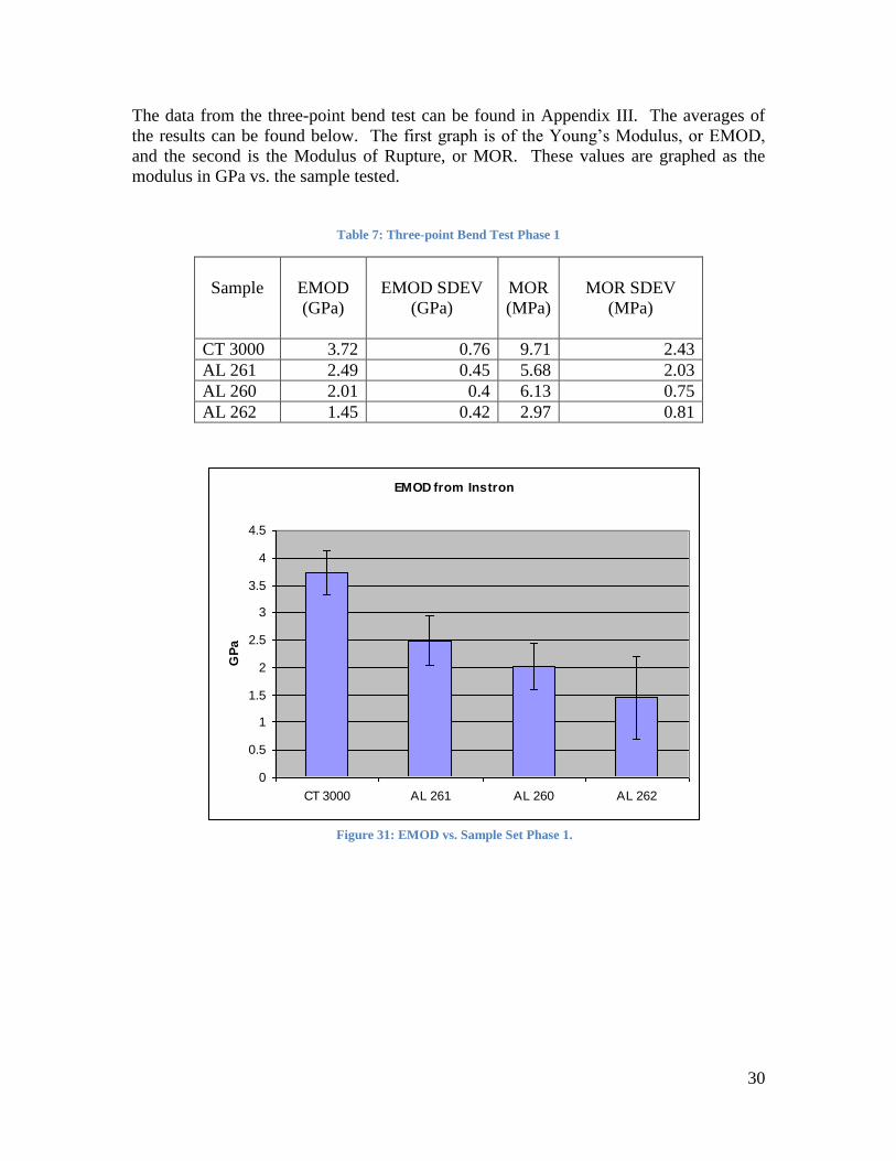
30

The data from the three-point bend test can be found in Appendix III. The averages of

the results can be found below. The first graph is of the Young‟s Modulus, or EMOD,

and the second is the Modulus of Rupture, or MOR. These values are graphed as the

modulus in GPa vs. the sample tested.

Table 7: Three-point Bend Test Phase 1

Sample

EMOD

(GPa)

EMOD SDEV

(GPa)

MOR

(MPa)

MOR SDEV

(MPa)

CT 3000 3.72 0.76 9.71 2.43

AL 261 2.49 0.45 5.68 2.03

AL 260 2.01 0.4 6.13 0.75

AL 262 1.45 0.42 2.97 0.81

EMOD from Instron

0

0.5

1

1.5

2

2.5

3

3.5

4

4.5

CT 3000 AL 261 AL 260 AL 262

GP

a

Figure 31: EMOD vs. Sample Set Phase 1.

31

Grindo-sonic values were recorded for the varied particle size alumina foam wheels.

Note that the inner diameter has not yet been drilled out, yet the equation being used calls

for this measurement.

Table 8: Wheel Grindo-sonic Values – Phase 1

Sample O.D

(in.)

I.D.

(in.)

Thickness

(in.)

Weight

(g)

Grindo

Sonic

Wt/Vol

Young’s

Modulus

(GPa)

AL260 1.960 0.000 1.124 50.72 71 0.913 4.655

AL260 1.960 0.000 1.121 50.48 71 0.911 4.727

AL260 1.960 0.000 1.130 49.96 73 0.894 4.167

AVE 4.52

STDEV 0.30

AL261 1.960 0.000 1.124 65.75 59 1.183 8.739

AL261 1.960 0.000 1.136 56.56 60 1.007 6.706

AL261 1.960 0.000 1.122 57.98 60 1.045 7.551

AVE 7.67

STDEV 1.02

AL262 1.920 0.000 0.975 54.78 75 1.184 10.144

AL262 1.920 0.000 0.967 53.73 79 1.171 9.381

AL262 1.920 0.000 0.935 49.40 81 1.113 9.760

AVE 9.76

STDEV 0.38

Measurements using the Grindo-sonic were also taken on 1x1/2x4in. bars using a

modified equation. Note that there is no value for AL261 and only one value for the

MOR

0

2

4

6

8

10

12

14

CT 3000 AL 261 AL 260 AL 262

MP

a

Figure 32: MOR vs. Sample Set – Phase 1.

32

other foams because there was not a piece of sample large enough to make one or

multiple bars.

Table 9: Bar Grindo-sonic Values - Phase 1

Sample

Weight

(g)

Grindo-

sonic

Density

(g/cc)

EMOD

(GPa)

AL262 33.27 538 1.015 10

CT3000 35.72 416 1.090 18

AL260 26.08 400 0.796 14

Figure 33: Young's Modulus vs. Sample from Bar Grindo-sonic Values – Phase 1

The results from the crush test are below; the first graph is of load or force being applied

to the foam versus time. The initial fracture can be seen, followed by a section of

multiple fractures as each layer is being broken, and then an exponential increase at the

end where the foam is compressed.

0.000

2.000

4.000

6.000

8.000

10.000

12.000

14.000

16.000

18.000

20.000

CT3000 AL260 AL262

Yo

un

g's

Mo

du

lus (

GP

a)

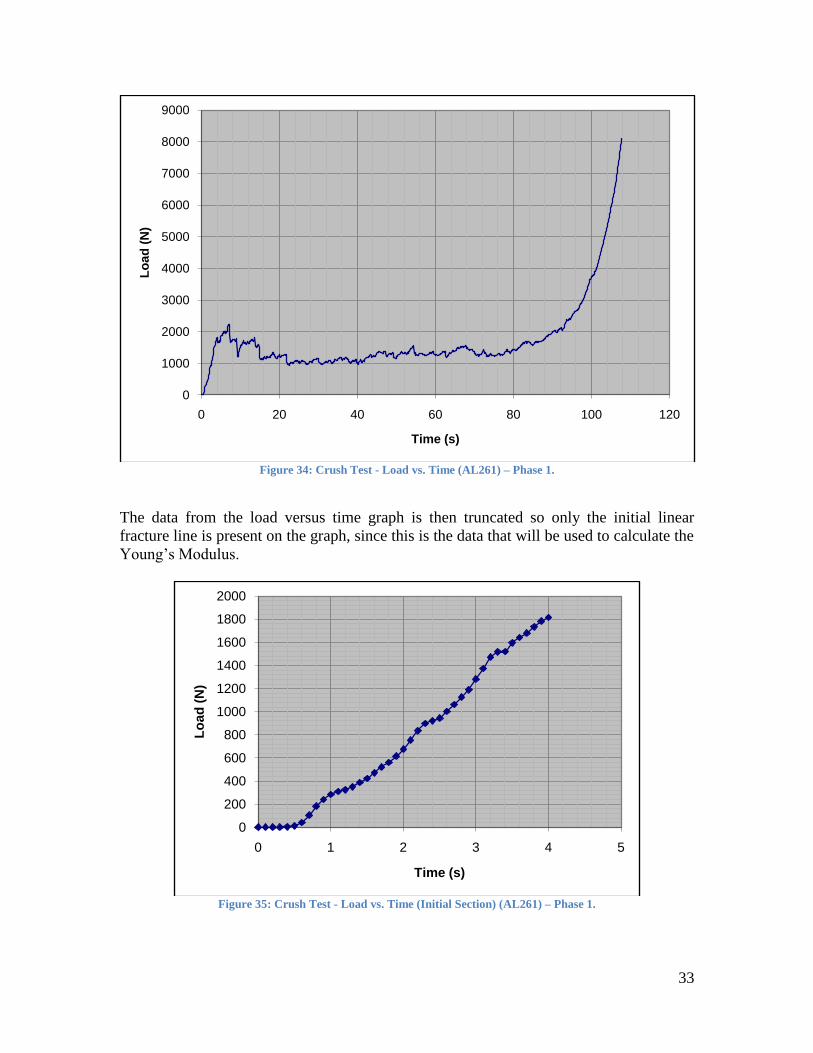
33

Figure 34: Crush Test - Load vs. Time (AL261) – Phase 1.

The data from the load versus time graph is then truncated so only the initial linear

fracture line is present on the graph, since this is the data that will be used to calculate the

Young‟s Modulus.

Figure 35: Crush Test - Load vs. Time (Initial Section) (AL261) – Phase 1.

0

1000

2000

3000

4000

5000

6000

7000

8000

9000

0 20 40 60 80 100 120

Lo

ad

(N

)

Time (s)

0

200

400

600

800

1000

1200

1400

1600

1800

2000

0 1 2 3 4 5

Lo

ad

(N

)

Time (s)

34

The data from Figure 36 is then converted into a Stress vs. Strain graph, where the

equation of the line is calculated, and the slope is taken as the Young‟s Modulus of the

foam in Pascals.

Figure 36: Crush Test - Stress vs. Strain (AL261) – Phase 1.

5.2 Physical Properties - Phase 1

5.2.1 Scanning Electron Microscope Analysis - Phase 1

The results from the SEM analysis are below, where the particles and the porosity of the

foam are investigated. For the porosity, both the macropores and the interconnected

pores have been measured using the Orion Software, where the length is calibrated using

the measurement in the legend of the picture.

The first set of data is from CT3000, where the large range of macropores can be seen, as

well as the large interconnected porosity.

y = 4E+08x - 2E+07

-2000000

0

2000000

4000000

6000000

8000000

10000000

12000000

14000000

0 0.01 0.02 0.03 0.04 0.05 0.06 0.07

Str

ess (

N/m

^2)

Strain

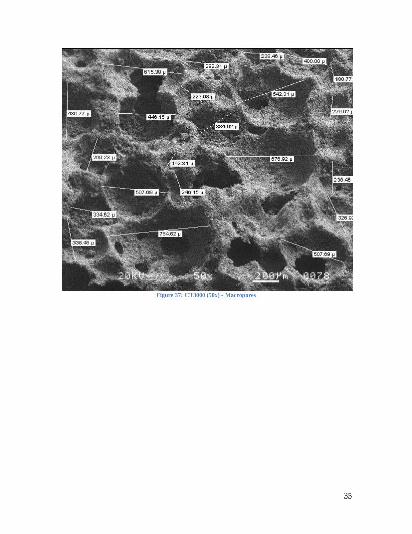
35

Figure 37: CT3000 (50x) - Macropores

36

Figure 38: CT 3000 (50x) Interconnected Pores.

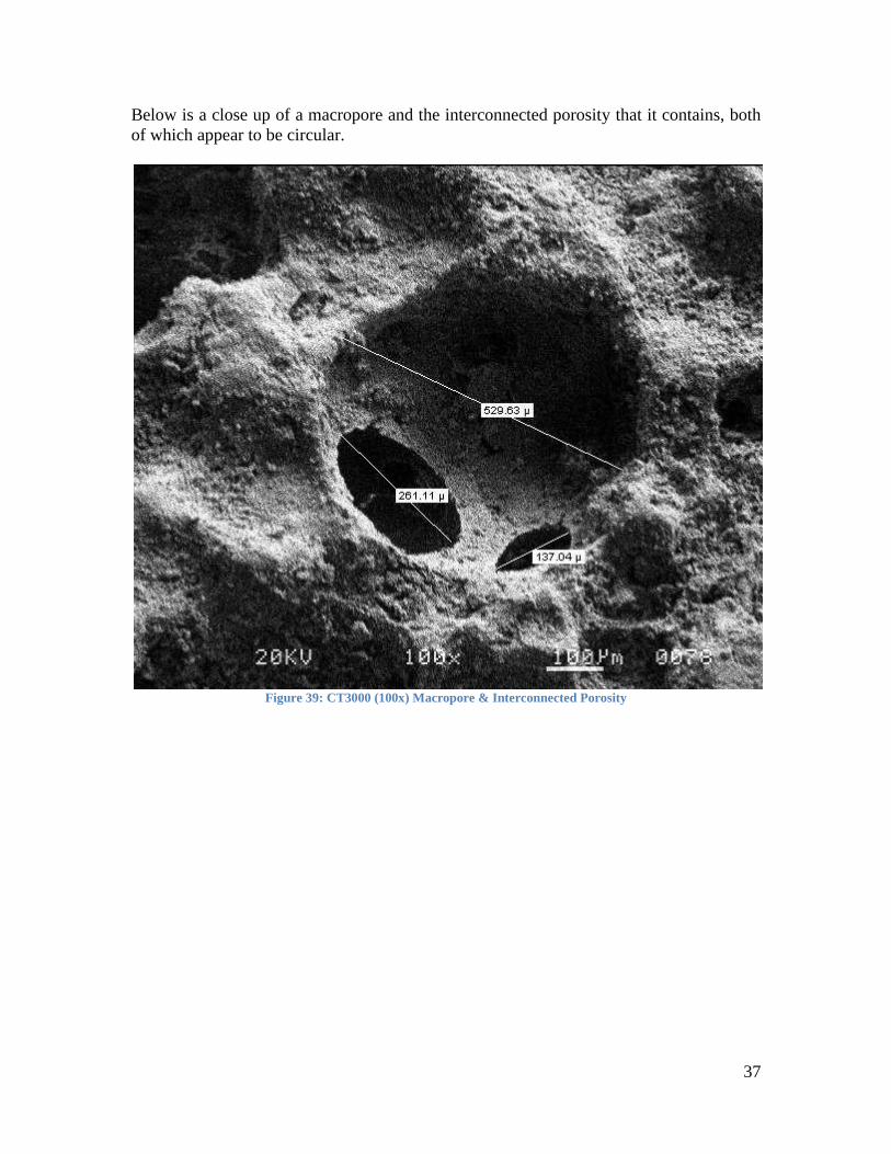
37

Below is a close up of a macropore and the interconnected porosity that it contains, both

of which appear to be circular.

Figure 39: CT3000 (100x) Macropore & Interconnected Porosity

38

In Figure 40 particles can be seen and can be measured. This section of the foam appears

to be a wall between two pores. The particles seem to be evenly distributed, although it

is hard to say at this magnification.

Figure 40: CT3000 (500x) Particle Size

39

The data for AL260 follows, which contains 50% 1µm and 50% 50µm particles. The

same macropore and interconnected porosity measurements were made.

Figure 41: AL260 (50x) Macropores.

40

Figure 42: AL260 (50x) Interconnected Pores.

41

In Figure 43 a large 50µm particle can be seen, surrounded by smaller particles. In this

area the particles seem to be evenly distributed. Also, there are some particles that are

measured in between the two starting particle sizes.

Figure 43: AL260 (1000x) Large Particle.

42

In Figure 44 a close up of a pore and the wall next to it can be seen. The pore seems to

be relatively small in size, and there appears to be an agglomeration of larger particles

beside the opening of the pore.

Figure 44: AL260 (1000x) Particle and Pore Size.

43

Another wall is pictured where the particles range in size with good distribution. The

largest particle measured is about 26.92µm and appears to have different layers that have

been fused together.

Figure 45: AL260 (1000x) Particle Size.

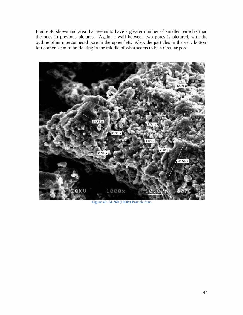
44

Figure 46 shows and area that seems to have a greater number of smaller particles than

the ones in previous pictures. Again, a wall between two pores is pictured, with the

outline of an interconnectd pore in the upper left. Also, the particles in the very bottom

left corner seem to be floating in the middle of what seems to be a circular pore.


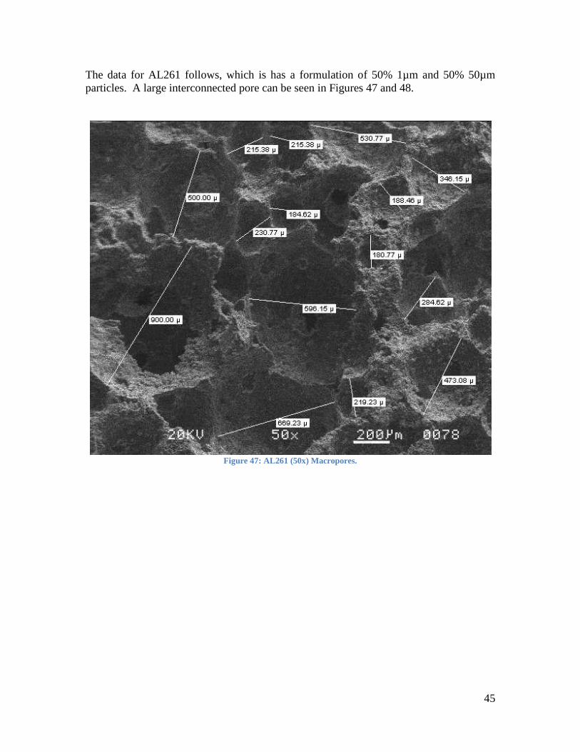
45

The data for AL261 follows, which is has a formulation of 50% 1µm and 50% 50µm

particles. A large interconnected pore can be seen in Figures 47 and 48.


46


47

Below is a picture of a pore and its interconnected pore in the bottom. The particles

through the interconnected pore are blurry, however it can be seen that the interconnected

porosity does indeed connect two pores together. There is also a large particle that

appears near the bottom of the pore.

Figure 49: AL261 (1000x) Particle and Innterconnected Pore.

48

Figure 50 is a close up of the particles, showing that the particles have sintered together

to create larger particles. However in this area there appears to only be 1µm particles that

have stayed the same size or have sintered together, and none of the larger 20µm

particles.


49

The data for AL262 follows, which is comprised of 50% 1µm and 50% 100µm particles.

There is a very large macropore pictured, as well as a very large interconnected pore.


50


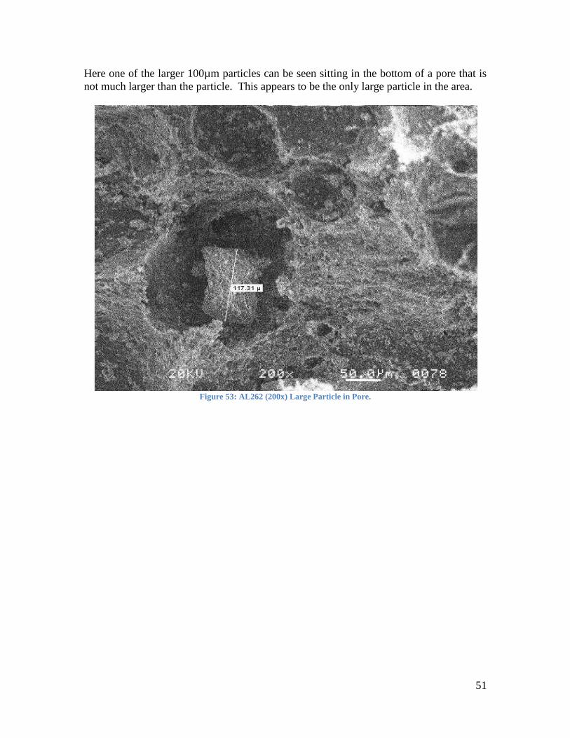
51

Here one of the larger 100µm particles can be seen sitting in the bottom of a pore that is

not much larger than the particle. This appears to be the only large particle in the area.

Figure 53: AL262 (200x) Large Particle in Pore.

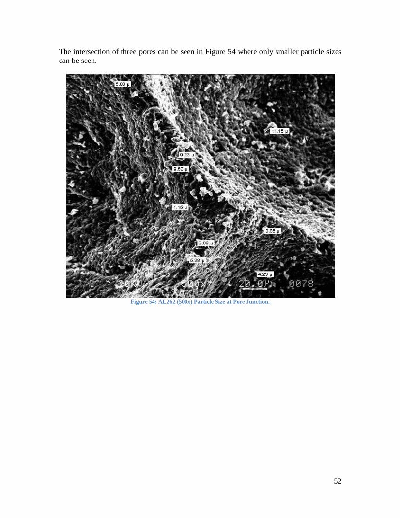
52

The intersection of three pores can be seen in Figure 54 where only smaller particle sizes

can be seen.

Figure 54: AL262 (500x) Particle Size at Pore Junction.

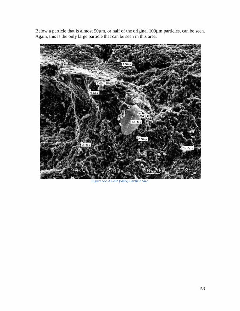
53

Below a particle that is almost 50µm, or half of the original 100µm particles, can be seen.

Again, this is the only large particle that can be seen in this area.


54

All of the data from the measured macropores and interconnected pores was averaged

and plotted. The average pore size is relatively constant across the different samples with

a large standard deviation.

Average Pore Size

0.00

100.00

200.00

300.00

400.00

500.00

600.00

260 261 262 CT3000

m*1

0^-6

Series1

Average Interconnected Pore Size

0.00

50.00

100.00

150.00

200.00

250.00

260 261 262 CT3000

m*1

0^-6

Series1

Figure 57: Interconnected Pore Size vs. Sample – Phase 1.

Figure 56: Average Pore Size (µm) vs. Sample – Phase 1.

55

5.2.2 CT Scan – Phase 1

The pore size ranges recorded for each of the samples scanned can be found in Table 10.

Table 10: Pore Size Range from CT Scan – Phase 1

Sample Pore size Range (µm)

CT 3000 #1 100 – 2500 (most under 1000)

CT 3000 #2 100 – 2500 (most under 1000)

CT 3000 #3 100 - 3600

In Figures 58-60 the images for each of the samples can be seen. There are four different

views; one from a top view, two from a side view at two different depths, and one

isometric view. These different views give an idea of the porosity distribution throughout

the samples.

Figure 58: CT Scan – Phase 1 (CT3000 #1).

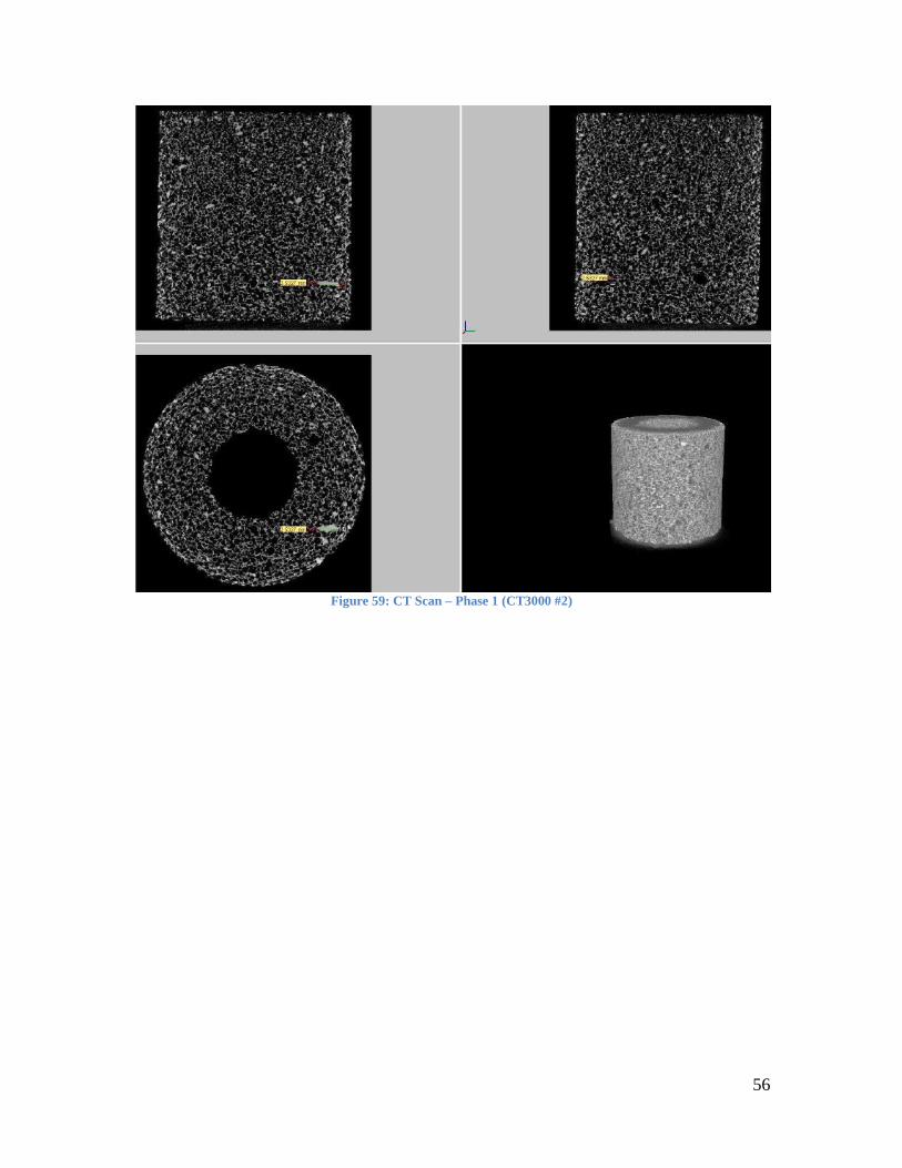
56

Figure 59: CT Scan – Phase 1 (CT3000 #2)

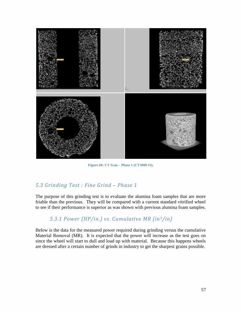
57

Figure 60: CT Scan – Phase 1 (CT3000 #3).

5.3 Grinding Test : Fine Grind – Phase 1

The purpose of this grinding test is to evaluate the alumina foam samples that are more

friable than the previous. They will be compared with a current standard vitrified wheel

to see if their performance is superior as was shown with previous alumina foam samples.

5.3.1 Power (HP/in.) vs. Cumulative MR (in3/in)

Below is the data for the measured power required during grinding versus the cumulative

Material Removal (MR). It is expected that the power will increase as the test goes on

since the wheel will start to dull and load up with material. Because this happens wheels

are dressed after a certain number of grinds in industry to get the sharpest grains possible.

58

Figure 61: Phase 1 - Power (Standard #1). Figure 62: Phase 1: Power (Standard #2).

Figure 63: Phase 1 - Power (CT3000 #2). Figure 64: Phase 1 - Power (CT3000 #3).

Figure 65: Phase 1 - Power (AL260#1). Figure 66: Phase 1 - Power (AL260#2).

0.00

0.50

1.00

1.50

2.00

2.50

3.00

3.50

0.00 0.02 0.04 0.06 0.08Cum. MR' [in³/in]

P' [

Hp

/in

]

DG 100 428-4-1

0.0

1.0

2.0

3.0

4.0

5.0

6.0

7.0

8.0

9.0

0.00 0.02 0.04 0.06 0.08Cum. MR' [in³/in]

P' [H

p/i

n]

DG 100 428-4-2

0.0

1.0

2.0

3.0

4.0

5.0

6.0

7.0

8.0

9.0

0.00 0.02 0.04 0.06 0.08Cum. MR' [in³/in]

P' [H

p/i

n]

CT 3000 #2

0.0

1.0

2.0

3.0

4.0

5.0

6.0

7.0

8.0

9.0

0.00 0.02 0.04 0.06 0.08Cum. MR' [in³/in]

P' [H

p/i

n]

CT 3000 #3

0.0

1.0

2.0

3.0

4.0

5.0

6.0

7.0

8.0

9.0

0.00 0.02 0.04 0.06 0.08Cum. MR' [in³/in]

P' [H

p/i

n]

AL 260 #1

0.0

1.0

2.0

3.0

4.0

5.0

6.0

7.0

8.0

9.0

0.00 0.02 0.04 0.06 0.08Cum. MR' [in³/in]

P' [H

p/i

n]

AL 260 #2

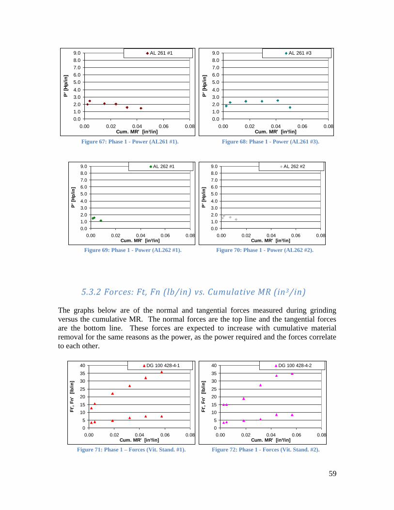
59

Figure 67: Phase 1 - Power (AL261 #1). Figure 68: Phase 1 - Power (AL261 #3).

Figure 69: Phase 1 - Power (AL262 #1). Figure 70: Phase 1 - Power (AL262 #2).

5.3.2 Forces: Ft, Fn (lb/in) vs. Cumulative MR (in3/in)

The graphs below are of the normal and tangential forces measured during grinding

versus the cumulative MR. The normal forces are the top line and the tangential forces

are the bottom line. These forces are expected to increase with cumulative material

removal for the same reasons as the power, as the power required and the forces correlate

to each other.

Figure 71: Phase 1 – Forces (Vit. Stand. #1). Figure 72: Phase 1 - Forces (Vit. Stand. #2).

0.0

1.0

2.0

3.0

4.0

5.0

6.0

7.0

8.0

9.0

0.00 0.02 0.04 0.06 0.08Cum. MR' [in³/in]

P' [H

p/i

n]

AL 261 #1

0.0

1.0

2.0

3.0

4.0

5.0

6.0

7.0

8.0

9.0

0.00 0.02 0.04 0.06 0.08Cum. MR' [in³/in]

P' [H

p/i

n]

AL 261 #3

0.0

1.0

2.0

3.0

4.0

5.0

6.0

7.0

8.0

9.0

0.00 0.02 0.04 0.06 0.08Cum. MR' [in³/in]

P' [H

p/i

n]

AL 262 #1

0.0

1.0

2.0

3.0

4.0

5.0

6.0

7.0

8.0

9.0

0.00 0.02 0.04 0.06 0.08Cum. MR' [in³/in]

P' [H

p/i

n]

AL 262 #2

0

5

10

15

20

25

30

35

40

0.00 0.02 0.04 0.06 0.08Cum. MR' [in³/in]

Ft',

Fn

' [

lb/i

n]

DG 100 428-4-1

0

5

10

15

20

25

30

35

40

0.00 0.02 0.04 0.06 0.08Cum. MR' [in³/in]

Ft',

Fn

' [

lb/i

n]

DG 100 428-4-2

60

Figure 73: Phase 1 - Forces (CT3000 #2). Figure 74: Phase 1 - Forces (CT3000 #3).

Figure 75: Phase 1 - Forces (AL260 #1). Figure 76: Phase 1 - Forces (AL260 #2).


0

5

10

15

20

25

30

35

40

0.00 0.02 0.04 0.06 0.08Cum. MR' [in³/in]

Ft',

Fn

' [

lb/i

n]

CT 3000 #2

0

5

10

15

20

25

30

35

40

0.00 0.02 0.04 0.06 0.08Cum. MR' [in³/in]

Ft',

Fn

' [

lb/i

n]

CT 3000 #3

0

5

10

15

20

25

30

35

40

0.00 0.02 0.04 0.06 0.08Cum. MR' [in³/in]

Ft',

Fn

' [

lb/i

n]

AL 260 #1

0

5

10

15

20

25

30

35

40

0.00 0.02 0.04 0.06 0.08Cum. MR' [in³/in]

Ft',

Fn

' [

lb/i

n]

AL 260 #2

0

5

10

15

20

25

30

35

40

0.00 0.02 0.04 0.06 0.08Cum. MR' [in³/in]

Ft',

Fn

' [

lb/i

n]

AL 261 #1

0

5

10

15

20

25

30

35

40

0.00 0.02 0.04 0.06 0.08Cum. MR' [in³/in]

Ft',

Fn

' [

lb/i

n]

AL 261 #3

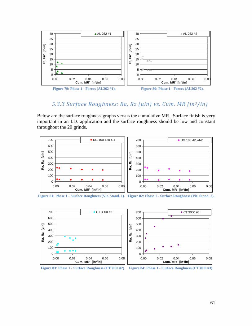
61


5.3.3 Surface Roughness: Ra, Rz (µin) vs. Cum. MR (in3/in)

Below are the surface roughness graphs versus the cumulative MR. Surface finish is very

important in an I.D. application and the surface roughness should be low and constant

throughout the 20 grinds.

Figure 81: Phase 1 - Surface Roughness (Vit. Stand. 1). Figure 82: Phase 1 - Surface Roughness (Vit. Stand. 2).

Figure 83: Phase 1 - Surface Roughness (CT3000 #2). Figure 84: Phase 1 - Surface Roughness (CT3000 #3).

0

5

10

15

20

25

30

35

40

0.00 0.02 0.04 0.06 0.08Cum. MR' [in³/in]

Ft',

Fn

' [

lb/i

n]

AL 262 #1

0

5

10

15

20

25

30

35

40

0.00 0.02 0.04 0.06 0.08Cum. MR' [in³/in]

Ft',

Fn

' [

lb/i

n]

AL 262 #2

0

100

200

300

400

500

600

700

0.00 0.02 0.04 0.06 0.08Cum. MR' [in³/in]

Ra,

Rz

[µin

]

DG 100 428-4-1

0

100

200

300

400

500

600

700

0.00 0.02 0.04 0.06 0.08Cum. MR' [in³/in]

Ra,

Rz

[µin

]

DG 100 428-4-2

0

100

200

300

400

500

600

700

0.00 0.02 0.04 0.06 0.08Cum. MR' [in³/in]

Ra,

Rz

[µin

]

CT 3000 #2

0

100

200

300

400

500

600

700

0.00 0.02 0.04 0.06 0.08Cum. MR' [in³/in]

Ra,

Rz

[µin

]

CT 3000 #3

62

Figure 85: Phase 1 - Surface Roughness (AL260 #1). Figure 86: Phase 1 - Surface Roughness (AL260 #2).



5.3.4 Surface Waviness: Wa, Wt (µin) vs. Cum. MR (in3/in)

Below is the data for surface waviness versus the cumulative MR. The surface waviness

is also very important for an I.D. grinding application and should have a low and constant

value throughout the test.

0

100

200

300

400

500

600

700

0.00 0.02 0.04 0.06 0.08Cum. MR' [in³/in]

Ra,

Rz

[µin

]

AL 260 #1

0

100

200

300

400

500

600

700

0.00 0.02 0.04 0.06 0.08Cum. MR' [in³/in]

Ra,

Rz

[µin

]

AL 260 #2

0

100

200

300

400

500

600

700

0.00 0.02 0.04 0.06 0.08Cum. MR' [in³/in]

Ra,

Rz

[µin

]

AL 261 #1

0

100

200

300

400

500

600

700

0.00 0.02 0.04 0.06 0.08Cum. MR' [in³/in]

Ra,

Rz

[µin

]

AL 261 #3

0

100

200

300

400

500

600

700

0.00 0.02 0.04 0.06 0.08Cum. MR' [in³/in]

Ra,

Rz

[µin

]

AL 262 #1

0

100

200

300

400

500

600

700

0.00 0.02 0.04 0.06 0.08Cum. MR' [in³/in]

Ra,

Rz

[µin

]

AL 262 #2

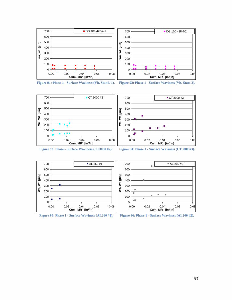
63

Figure 91: Phase 1 - Surface Waviness (Vit. Stand. 1). Figure 92: Phase 1 - Surface Waviness (Vit. Stan. 2).

Figure 93: Phase - Surface Waviness (CT3000 #2). Figure 94: Phase 1 - Surface Waviness (CT3000 #3).

Figure 95: Phase 1 - Surface Waviness (AL260 #1). Figure 96: Phase 1 - Surface Waviness (AL260 #2).

0

100

200

300

400

500

600

700

0.00 0.02 0.04 0.06 0.08Cum. MR' [in³/in]

Wa,

Wt

[µ

in]

DG 100 428-4-1

0

100

200

300

400

500

600

700

0.00 0.02 0.04 0.06 0.08Cum. MR' [in³/in]

Wa,

Wt

[µ

in]

DG 100 428-4-2

0

100

200

300

400

500

600

700

0.00 0.02 0.04 0.06 0.08Cum. MR' [in³/in]

Wa,

Wt

[µ

in]

CT 3000 #2

0

100

200

300

400

500

600

700

0.00 0.02 0.04 0.06 0.08Cum. MR' [in³/in]

Wa,

Wt

[µ

in]

CT 3000 #3

0

100

200

300

400

500

600

700

0.00 0.02 0.04 0.06 0.08Cum. MR' [in³/in]

Wa,

Wt

[µ

in]

AL 260 #1

0

100

200

300

400

500

600

700

0.00 0.02 0.04 0.06 0.08Cum. MR' [in³/in]

Wa,

Wt

[µ

in]

AL 260 #2

64



5.3.5 Wheel Wear – Phase 1

During grinding, wheels should wear down in order to expose sharper grains. However,

if the wheels wear too fast, then they will only be able to grind a few numbers of times

and would not be cost effective. Below in Table 11 is the recorded wheel wear data for

the wheels tested during the find grind in the grinding Test 1.

0

100

200

300

400

500

600

700

0.00 0.02 0.04 0.06 0.08Cum. MR' [in³/in]

Wa,

Wt

[µ

in]

AL 261 #1

0

100

200

300

400

500

600

700

0.00 0.02 0.04 0.06 0.08Cum. MR' [in³/in]

Wa,

Wt

[µ

in]

AL 261 #3

0

100

200

300

400

500

600

700

0.00 0.02 0.04 0.06 0.08Cum. MR' [in³/in]

Wa,

Wt

[µ

in]

AL 262 #1

0

100

200

300

400

500

600

700

0.00 0.02 0.04 0.06 0.08Cum. MR' [in³/in]

Wa,

Wt

[µ

in]

AL 262 #2

65

Table 11: Wheel Wear – Phase 1

Specification Rad. Wheel Wear (in.)

DG 100 428-4-1 0.0001

DG 100 428-4-1 0.00015

CT3000 #2 0.00815

CT3000 #3 0.0099

AL261 #1 0.01

AL261 #3 0.00893

AL260 #2 0.0109

AL260 #1 0.01160 (10 grinds)

AL262 #2 0.01280 (15 grinds)

AL262 #1 0.00800 (5 grinds)

5.4 Grinding Test: Rough Grind – Phase 1 The main reason for performing this grind test is to evaluate how the samples perform in

the rough rate. The samples were made more friable so they would theoretically perform

well in the rough grind without loading up with metal as was observed in the previous

alumina foam samples. Note there is only data from the standard vitrified wheel as the

wheel wear for the alumina foam samples was too high to perform a rough grind.

5.4.1 Power (HP/in.) vs. Cumulative MR (in3/in)

Below is the data for power versus the cumulative MR. This power typically increases

with increasing cumulative MR.

Figure 101: Phase 1 - Rough - Power (Vit. 1). Figure 102: Phase 1 - Rough - Power (Vit. 2).

0.0

1.0

2.0

3.0

4.0

5.0

6.0

7.0

8.0

9.0

0.00 0.10 0.20 0.30 0.40Cum. MR' [in³/in]

P' [H

p/i

n]

DG 100 428-4-1

0.0

1.0

2.0

3.0

4.0

5.0

6.0

7.0

8.0

9.0

0.00 0.10 0.20 0.30 0.40Cum. MR' [in³/in]

P' [H

p/i

n]

DG 100 428-4-2

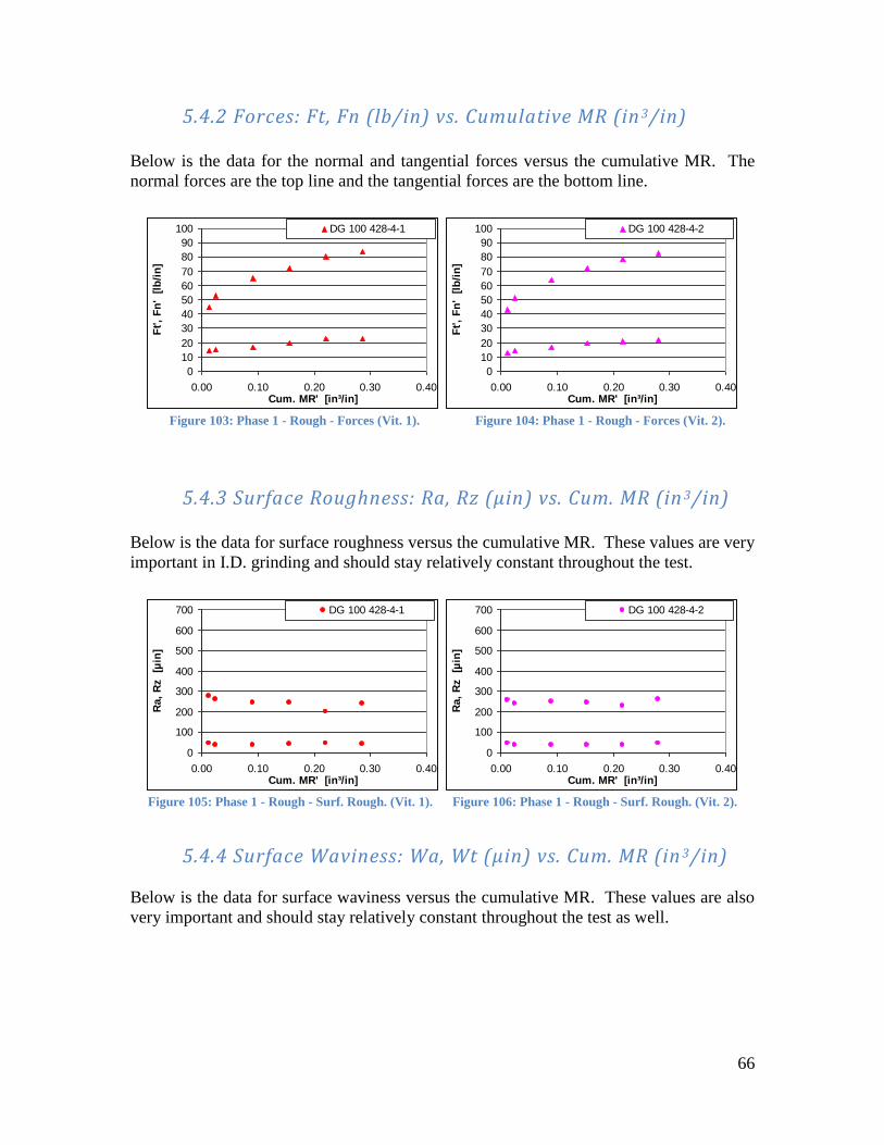
66

5.4.2 Forces: Ft, Fn (lb/in) vs. Cumulative MR (in 3/in) Below is the data for the normal and tangential forces versus the cumulative MR. The

normal forces are the top line and the tangential forces are the bottom line.

Figure 103: Phase 1 - Rough - Forces (Vit. 1). Figure 104: Phase 1 - Rough - Forces (Vit. 2).

5.4.3 Surface Roughness: Ra, Rz (µin) vs. Cum. MR (in 3/in) Below is the data for surface roughness versus the cumulative MR. These values are very

important in I.D. grinding and should stay relatively constant throughout the test.

Figure 105: Phase 1 - Rough - Surf. Rough. (Vit. 1). Figure 106: Phase 1 - Rough - Surf. Rough. (Vit. 2).

5.4.4 Surface Waviness: Wa, Wt (µin) vs. Cum. MR (in 3/in)

Below is the data for surface waviness versus the cumulative MR. These values are also

very important and should stay relatively constant throughout the test as well.

0

10

20

30

40

50

60

70

80

90

100

0.00 0.10 0.20 0.30 0.40Cum. MR' [in³/in]

Ft',

Fn

' [

lb/i

n]

DG 100 428-4-1

0

10

20

30

40

50

60

70

80

90

100

0.00 0.10 0.20 0.30 0.40Cum. MR' [in³/in]

Ft',

Fn

' [

lb/i

n]

DG 100 428-4-2

0

100

200

300

400

500

600

700

0.00 0.10 0.20 0.30 0.40Cum. MR' [in³/in]

Ra,

Rz

[µin

]

DG 100 428-4-1

0

100

200

300

400

500

600

700

0.00 0.10 0.20 0.30 0.40Cum. MR' [in³/in]

Ra,

Rz

[µin

]

DG 100 428-4-2

67

Figure 107: Phase 1 - Rough - Surf. Wav. (Vit. 1). Figure 108: Phase 1 - Rough - Surf. Wav. (Vit. 2).

5.5 Mechanical Properties – Phase 2

The values for density, Grindo-sonic, and Young‟s Modulus are below in Table 11 for

1x1/2x4 in. bars

Table 12: Mechanical Properties – Phase 2

Sample

Weight

(g)

Grindo

Sonic

Density

(g/cc)

Bulk

Density

(g/cc)

EMOD

(GPa)

356A #1 49.24 272 1.502 56.5

356A #2 48.55 272 1.481 55.7

356A #3 48.97 274 1.494 55.3

AVG 1.49 1.54 55.82

STDEV 0.01 0.58

356B #1 49.31 278 1.504 54.1

356B #2 50.10 282 1.528 53.4

356B #3 50.48 275 1.528 56.2

AVG 1.52 1.55 54.59

STDEV 0.01 1.44

356C #1 49.97 311 1.524 44.0

356C #2 48.88 272 1.491 56.1

356C #3 52.19 298 1.592 49.9

AVG 1.54 1.50 49.97

STDEV 0.05 6.03

356D #1 51.24 297 1.563 49.3

356D #2 51.96 283 1.585 55.0

356D #3 50.80 310 1.550 44.8

AVG 1.57 1.46 49.72

STDEV 0.02 5.11

From the measured density the porosity of the wheel was calculated using the known

density of alumina to be 3.97g/cc.

0

100

200

300

400

500

600

700

0.00 0.10 0.20 0.30 0.40Cum. MR' [in³/in]

Wa,

Wt

[µ

in]

DG 100 428-4-1

0

100

200

300

400

500

600

700

0.00 0.10 0.20 0.30 0.40Cum. MR' [in³/in]

Wa,

Wt

[µ

in]

DG 100 428-4-2

68

Table 13: Calulated Porosity – Phase 2

Specification

Measured

Density

(g/cc)

Porosity

(%)

356A #1 1.50 62

356A #2 1.48 63

356A #3 1.49 62

AVE 62

STDEV 0.3

356B #1 1.50 62

356B #2 1.53 62

356B #3 1.53 62

AVE 62

STDEV 0.3

356C #1 1.52 62

356C #2 1.49 62

356C #3 1.59 60

AVE 61

STDEV 1.3

356D #1 1.56 61

356D #2 1.59 60

356D #3 1.55 61

AVE 61

STDEV 0.4

Figure 109: Porosity vs. Sample - Phase 2.

58

58.5

59

59.5

60

60.5

61

61.5

62

62.5

356A 356B 356C 356D

Po

rosit

y (

%)

69

5.6 Physical Properties – Phase 2

5.6.1 Scanning Electron Microscope Analysis – Phase 2

The results from the SEM analysis are below, where the particles and the porosity of the

foam are investigated. For the porosity, both the macropores and the interconnected

pores have been measured using the Orion Software, where the length is calibrated using

the measurement in the legend of the picture.

The data for 356A, with a sintering temperature of 1700°C, follows. In Figures 110 and

112 there seems to be a group of smaller macropores throughout the center surrounded by

larger macropores.

Figure 110: 356A (50x) Macropores.

70

Figure 111: 356A (50x) Interconnected Pores.

71

In Figure 112 it appears that there are some striations on the surface of the foam, which is

from cutting the foam to obtain the sample for the SEM. There also appear to be some

small particles in the pores, about 6-7µm.

Figure 112: 356A (200x) Arrow points to striations.

72

Figure 113 shows the sintering behavior of the particles. It appears that larger particles

have been sintered together, as well as smaller particles on the surface.

Figure 113: 356A (3000x).

73

Below is the data for 356B which was sintered at 1680°C. This foam appears to have

clusters of smaller macropores evenly dispersed throughout the larger macropores,

similar to 356A.

Figure 114: 356B (50x) Macropores.

74

Figure 115: 356B (50x) Interconnected Pores.

75

In Figure 116 a very large particle, about 151µm in size, is seen in the bottom of a large

macropore.

Figure 116: 356B (100x) Large Particle.

76

Figure 117 shows a similar structure to 356A, where larger particles are sintered together

with smaller particles in the surface.

Figure 117: 356B (3000x).

77

The sample 356C was sintered at 1630°C, the same sintering temperature used for the

phase 1 samples. The structure of these samples can be seen in the following pictures.

In Figures 118 and 119 an even distribution of porosity can be seen.

Figure 118: 356C (50x) Macropores.

78

Figure 119: 356C (50x) Interconnected Pores.

79

In Figure 120 some smaller particles, about 20µm, can be seen in the bottom pores, as

well as some interconnected porosity.

Figure 120: 356C (100x).

80

Figure 121 is taken from the wall of a pore, and has larger particles sintered together with

a lot of smaller particles on the surface.

Figure 121: 356C (3000x).

81

The data for the 356D sample, which was sintered at 1590°C, is as follows. A similar

porosity distribution to the previous phase two samples can be seen, however the largest

macropores appear to be smaller than the other samples.

Figure 122: 356D (50x) Macropores.

82

Figure 123: 356D (50x) Interconnected Pores.

83

In Figure 124 large interconnected pores can be seen, one around 100µm and one around

143µm.

Figure 124: 356D (100x).

84

In Figure 125 it appears that the sintered particles are smaller in size than the previous

phase 2 samples. Also, there is a greater amount of particles on the surface, which seem

to be greater in size than the ones found in previous samples.

Figure 125: 356D (3000x).

5.6.2 CT Scan – Phase 2

The pore size ranges found with the CT Scan are shown below in for each of the samples.

Table 14: Pore Size Range from CT Scan - Phase 2

Sample Pore size Range (µm)

356A 100 - 3800

356B 100 - 2100

356C 100 - 3800

356D 100 - 2200

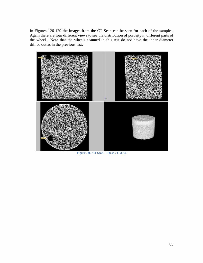
85

In Figures 126-129 the images from the CT Scan can be seen for each of the samples.

Again there are four different views to see the distribution of porosity in different parts of

the wheel. Note that the wheels scanned in this test do not have the inner diameter

drilled out as in the previous test.

Figure 126: CT Scan - Phase 2 (356A).

86

Figure 127: CT Scan - Phase 2 (356B).

Figure 128: CT Scan - Phase 2 (356C).

87

Figure 129: CT Scan - Phase 2 (356D).

5.7 Grinding Test : Fine Grind – Phase 2

The purpose of this test was to evaluate the repeatability of each sample set. Three

wheels from each specification were tested to determine which sintering cycle produced

the foam with the most evenly distributed porosity, or the most repeatable wheel.

5.7.1 Power (HP/in.) vs. Cumulative MR (in 3/in)

Below is the data for the measured power required during grinding versus the cumulative

Material Removal (MR). It is expected that the power will increase as the test goes on

since the wheel will start to dull and load up with material. Because this happens wheels

are dressed after a certain number of grinds in industry to get the sharpest grains possible.

88

Figure 130: Phase 2 - (356A #1). Figure 131: Phase 2 - Power (356A #2).

Figure 132: Phase 2 - Power (356A #3).

Figure 133: Phase 2 - Power (356B #1). Figure 134: Phase 2 - Power (356B #2).

Figure 135: Phase 2 - Power (356B #3).

0

1

2

3

4

5

6

7

8

9

0.00 0.02 0.04 0.06 0.08Cum. MR' [in³/in]

Un

it P

ow

er

[H

p/i

n]

A-1

0

1

2

3

4

5

6

7

8

9

0.00 0.02 0.04 0.06 0.08Cum. MR' [in³/in]

Un

it P

ow

er

[H

p/i

n]

A-2

0

1

2

3

4

5

6

7

8

9

0.00 0.02 0.04 0.06 0.08Cum. MR' [in³/in]

Un

it P

ow

er

[H

p/i

n]

A-3

0

1

2

3

4

5

6

7

8

9

0.00 0.02 0.04 0.06 0.08Cum. MR' [in³/in]

Un

it P

ow

er

[H

p/i

n]

B-1

0

1

2

3

4

5

6

7

8

9

0.00 0.02 0.04 0.06 0.08Cum. MR' [mm³/mm]

Un

it P

ow

er

[W

/mm

]

B-2

0

1

2

3

4

5

6

7

8

9

0.00 0.02 0.04 0.06 0.08Cum. MR' [in³/in]

Un

it P

ow

er

[H

p/i

n]

B-3

89

Figure 136: Phase 2 - Power (356C #1). Figure 137: Phase 2 - Power (356C #2).

Figure 138: Phase 2 - Power (356C #3).

Figure 139: Phase 2 - Power (356D #1). Figure 140: Phase 2 - Power (356D #2).

Figure 141: Phase 2 - Power (356D #3).

0

1

2

3

4

5

6

7

8

9

0.00 0.02 0.04 0.06 0.08Cum. MR' [in³/in]

Un

it P

ow

er

[H

p/i

n]

C-1

0

1

2

3

4

5

6

7

8

9

0.00 0.02 0.04 0.06 0.08Cum. MR' [in³/in]

Un

it P

ow

er

[H

p/i

n]

C-2

0

1

2

3

4

5

6

7

8

9

0.00 0.02 0.04 0.06 0.08Cum. MR' [in³/in]

Un

it P

ow

er

[H

p/i

n]

C-3

0

1

2

3

4

5

6

7

8

9

0.00 0.02 0.04 0.06 0.08Cum. MR' [in³/in]

Un

it P

ow

er

[H

p/i

n]

D-1

0

1

2

3

4

5

6

7

8

9

0.00 0.02 0.04 0.06 0.08Cum. MR' [in³/in]

Un

it P

ow

er

[H

p/i

n]

D-2

0

1

2

3

4

5

6

7

8

9

0.00 0.02 0.04 0.06 0.08Cum. MR' [in³/in]

Un

it P

ow

er

[H

p/i

n]

D-3

90

5.7.2 Forces: Ft, Fn (lb/in) vs. Cumulative MR (in 3/in)

The graphs below are of the normal and tangential forces measured during grinding

versus the cumulative MR. The normal forces are the top line and the tangential forces

are the bottom line. These forces are expected to increase with cumulative material

removal for the same reasons as the power, as the power required and the forces correlate

to each other.

Figure 142: Phase 2 - Forces (356A #1). Figure 143: Phase 2 - Forces (356A #2).

Figure 144: Phase 2 - Forces (356A #3).

Figure 145: Phase 2 - Forces (356B #1. Figure 146: Phase 2 - Forces (356B #2).

-20

0

20

40

60

80

100

0.00 0.02 0.04 0.06 0.08

Cum. MR' [in³/in]

Ft,

Fn

[l

b/i

n]

A-1

-20

0

20

40

60

80

100

0.00 0.02 0.04 0.06 0.08

Cum. MR' [in³/in]

Ft,

Fn

[l

b/i

n]

A-2

-20

0

20

40

60

80

100

0.00 0.02 0.04 0.06 0.08

Cum. MR' [in³/in]

Ft,

Fn

[l

b/i

n]

A-3

-20

0

20

40

60

80

100

0.00 0.02 0.04 0.06 0.08

Cum. MR' [in³/in]

Ft,

Fn

[l

b/i

n]

B-1

-20

0

20

40

60

80

100

0.00 0.02 0.04 0.06 0.08

Cum. MR' [in³/in]

Ft,

Fn

[l

b/i

n]

B-2

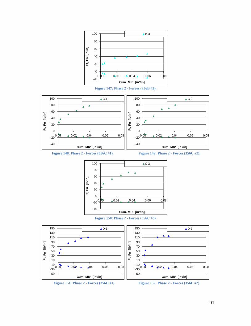
91

Figure 147: Phase 2 - Forces (356B #3).

Figure 148: Phase 2 - Forces (356C #1). Figure 149: Phase 2 - Forces (356C #2).

Figure 150: Phase 2 - Forces (356C #3).

Figure 151: Phase 2 - Forces (356D #1). Figure 152: Phase 2 - Forces (356D #2).

-20

0

20

40

60

80

100

0.00 0.02 0.04 0.06 0.08

Cum. MR' [in³/in]

Ft,

Fn

[l

b/i

n]

B-3

-40

-20

0

20

40

60

80

100

0.00 0.02 0.04 0.06 0.08

Cum. MR' [in³/in]

Ft,

Fn

[l

b/i

n]

C-1

-40

-20

0

20

40

60

80

100

0.00 0.02 0.04 0.06 0.08

Cum. MR' [in³/in]

Ft,

Fn

[l

b/i

n]

C-2

-40

-20

0

20

40

60

80

100

0.00 0.02 0.04 0.06 0.08

Cum. MR' [in³/in]

Ft,

Fn

[l

b/i

n]

C-3

-50

-30

-10

10

30

50

70

90

110

130

150

0.00 0.02 0.04 0.06 0.08

Cum. MR' [in³/in]

Ft,

Fn

[l

b/i

n]

D-1

-50

-30

-10

10

30

50

70

90

110

130

150

0.00 0.02 0.04 0.06 0.08

Cum. MR' [in³/in]

Ft,

Fn

[l

b/i

n]

D-2

92

Figure 153: Phase 2 - Forces (356D #3).

5.7.3 Surface Roughness: Ra, Rz (µin) vs. Cum. MR (in 3/in)

Below are the surface roughness graphs versus the cumulative MR. Surface finish is very

important in an I.D. application and the surface roughness should be low and constant

throughout the 20 grinds.

Figure 154: Phase 2 - Surface Roughness (356A #1). Figure 155: Phase 2 - Surface Roughness (356A #2).

Figure 156: Phase 2 - Surface Roughness (356A #3).

-50

-30

-10

10

30

50

70

90

110

130

150

0.00 0.02 0.04 0.06 0.08

Cum. MR' [in³/in]

Ft,

Fn

[l

b/i

n]

D-3

0

100

200

300

400

500

600

700

0.00 0.02 0.04 0.06 0.08Cum. MR' [in³/in]

Ra,

Rz

[µin

]

A-1

0

100

200

300

400

500

600

700

0.00 0.02 0.04 0.06 0.08Cum. MR' [in³/in]

Ra,

Rz

[µin

]

A-3

93

Figure 157: Phase 2 - Surface Roughness (356B #1). Figure 158: Phase 2 - Surface Roughness (356B #2).

Figure 159: Phase 2 - Surface Roughness (356B #3).

Figure 160: Phase 2 - Surface Roughness (356C #1). Figure 161: Phase 2 - Surface Roughness (356C #2).

Figure 162: Phase 2 - Surface Roughness (356C #3).

0

100

200

300

400

500

600

700

0.00 0.02 0.04 0.06 0.08Cum. MR' [in³/in]

Ra,

Rz

[µm

]

B-1

0

100

200

300

400

500

600

700

0.00 0.02 0.04 0.06 0.08Cum. MR' [in³/in]

Ra,

Rz

[µin

]

B-2

0

100

200

300

400

500

600

700

0.00 0.02 0.04 0.06 0.08Cum. MR' [in³/in]

Ra,

Rz

[µm

]

B-3

0

100

200

300

400

500

600

700

0.00 0.02 0.04 0.06 0.08Cum. MR' [in³/in]

Ra,

Rz

[µin

]

C-1

0

100

200

300

400

500

600

700

0.00 0.02 0.04 0.06 0.08Cum. MR' [in³/in]

Ra,

Rz

[µin

]

C-2

0

100

200

300

400

500

600

700

0.00 0.02 0.04 0.06 0.08Cum. MR' [in³/in]

Ra,

Rz

[µin

]

C-3

94

Figure 163: Phase 2 - Surface Roughness (356D #1). Figure 164: Phase 2 - Surface Roughness (356D #2).

Figure 165: Phase 2 - Surface Roughness (356D #3).

5.7.4 Surface Waviness: Wa, Wt (µin) vs. Cum. MR (in3/in)

Below is the data for surface waviness versus the cumulative MR. The surface waviness

is also very important for an I.D. grinding application and should have a low and constant

value throughout the test.

Figure 166: Phase 2 - Surface Waviness (356A #1). Figure 167: Phase 2 - Surface Waviness (356A #2).

0

100

200

300

400

500

600

700

0.00 0.02 0.04 0.06 0.08Cum. MR' [in³/in]

Ra,

Rz

[µin

]

D-1

0

100

200

300

400

500

600

700

0.00 0.02 0.04 0.06 0.08Cum. MR' [in³/in]

Ra,

Rz

[µin

]

D-2

0

100

200

300

400

500

600

700

0.00 0.02 0.04 0.06 0.08Cum. MR' [in³/in]

Ra,

Rz

[µin

]

D-3

0

100

200

300

400

500

600

700

0.00 0.02 0.04 0.06 0.08Cum. MR' [in³/in]

Wa,

Wt

[µ

in]

A-1

95

Figure 168: Phase 2 - Surface Waviness (356A #3).

Figure 169: Phase 2 - Surface Waviness (356B #1). Figure 170: Phase 2 - Surface Waviness (356B #2).

Figure 171: Phase 2 - Surface Waviness (356B #3).

Figure 172: Phase 2 - Surface Waviness (356C #1). Figure 173: Phase 2 - Surface Waviness (356C #2).

0

100

200

300

400

500

600

700

0.00 0.02 0.04 0.06 0.08Cum. MR' [in³/in]

Wa,

Wt

[µ

in]

A-3

0

100

200

300

400

500

600

700

0.00 0.02 0.04 0.06 0.08Cum. MR' [in³/in]

Wa,

Wt

[µ

in]

B-1

0

100

200

300

400

500

600

700

0.00 0.02 0.04 0.06 0.08Cum. MR' [in³/in]

Wa,

Wt

[µ

in]

B-2

0

100

200

300

400

500

600

700

0.00 0.02 0.04 0.06 0.08Cum. MR' [in³/in]

Wa,

Wt

[µ

in]

B-3

0

100

200

300

400

500

600

700

0.00 0.02 0.04 0.06 0.08Cum. MR' [in³/in]

Wa,

Wt

[µ

in]

C-1

0

100

200

300

400

500

600

700

0.00 0.02 0.04 0.06 0.08Cum. MR' [in³/in]

Wa,

Wt

[µ

in]

C-2

96

Figure 174: Phase 2 - Surface Waviness (356C #3).

Figure 175: Phase 2 - Surface Waviness (356D #1). Figure 176: Phase 2 - Surface Waviness (356D #2).

Figure 177: Phase 2 - Surface Waviness (356D #3).

5.7.5 Wheel Wear – Phase 2

During grinding, wheels wear should wear down in order to expose sharper grains.

However, if the wheels wear too fast, then they will only be able to grind a few numbers

of times and would not be cost effective. The wheel wear calculated during the grinding

test for the phase 2 samples is shown in Table 15.

0

100

200

300

400

500

600

700

0.00 0.02 0.04 0.06 0.08Cum. MR' [in³/in]

Wa,

Wt

[µ

in]

C-3

0

100

200

300

400

500

600

700

0.00 0.02 0.04 0.06 0.08Cum. MR' [in³/in]

Wa,

Wt

[µ

in]

D-1

0

100

200

300

400

500

600

700

0.00 0.02 0.04 0.06 0.08Cum. MR' [in³/in]

Wa,

Wt

[µ

in]

D-2

0

100

200

300

400

500

600

700

0.00 0.02 0.04 0.06 0.08Cum. MR' [in³/in]

Wa,

Wt

[µ

in]

D-3

97

Table 15: Wheel Wear – Phase 2

Sample

Wheel Wear

(in.)

356A #1 0.0015

356A #2 0.0010

356A #3 0.0010

356B #1 0.0014

356B #2 0.0010

356B #3 0.0010

356C #1 0.0015

356C #2 0.0015

356C #3 0.0013

356D #1 0.0015

356D #2 0.0020

356D #3 0.0020

98

6.0 Discussion


Quantifying the properties for alumina foam proved to be a challenge. The structure of

the foam is very different from current grinding wheels, which are less porous than the

foam and contain a matrix of bond and abrasive. Because of these differences some

standard tests had to be altered or disregarded.

The measured densities of the various foam samples were relatively close to the bulk

densities that were given. Although the CT3000 #3 sample was much lower than the

bulk density, at 0.87g/cc where the bulk density was 1.1g/cc. This means that the sample

is more porous.

From the calculated porosity the range was found to be 71 – 78% between the samples.

The CT3000 #3 samples had a high porosity of 78 as expected based on the density

calculations. The AL261 samples had the highest porosity, followed by 260, CT3000,

and then 262. The AL261 and AL262 samples have a lower standard deviation than the

AL260 and CT3000 samples, from 0.02 to 0.13 and 0.08 respectively. This means that it

should be expected that the AL260 samples would have a larger variation in the grinding

test results.

For calculating the Young‟s Modulus and the Modulus of Rupture, the typical test used

for current grinding wheels is the three point bend test using an Instron. The trend

usually seen is with a harder grade wheel, or a less friable wheel, the higher the Young‟s

Modulus. Also, the order of the modulus is usually in the GPa range, the modulus for the

previous alumina foam samples was recorded as 30GPa for a similar amount of porosity.

When the alumina foam samples were tested, they had values in the low GPa range, from

1.45 – 3.72, but did show a similar trend with the least friable sample having the highest

modulus. The same trend is usually seen for the Modulus of Rupture; however the

alumina foam samples did not seem to follow a trend. Also, after the test was completed,

it appeared that some of the samples did not break through the entire bar. The

explanation for this could be that the three point bend test puts a force on a single point,

and could be calculating data from the destruction of a single or multiple layers of the

foam and not the entire structure. This could produce lower than expected values and

could create data that does not seem to have a correlation if a different number of layers

were broken for the various samples. A better test for a foam would a crush test, which

would crush the entire structure.

The crush test is a more typical test for foams. The graph that was created from the

measured data from the Instron had a very similar curve to one typically found for brittle

compression, in fact it had less noise than the example. However, the Young‟s Modulus

values found with the crush test were significantly lower than those found with the three

point bend test, for AL261 on the order of 0.4GPa, or 400MPa. This could be due to the

99

small sample size that was used, and could have had failure due to the corners. However

the sample size was selected based on the capabilities of the machine. If a larger sample

were to be tested, such as 1x1x1in., a larger load would have to be used, which was not

available.

The Grindo-sonic test is the other test that is typically used for conventional wheels and

is cross-checked with the Instron values. At first, alumina foam wheels were tested,

which is a common practice. The highest value calculated was 9.76GPa for AL262, the

second highest was AL261, followed by AL260. This is not the trend that is expected,

AL261 should have the highest modulus and AL262 should have the lowest. Also, the

values obtained for the previous foams was a magnitude of ten higher, around 30GPa.

This could be due to the fact that the wheels were so small and light a repeatable value

could not be obtained.

Another Grindo-sonice test was performed on 1x½x4in. bars, which is also a common

practice. These samples seemed to provide better results, repeatable values could be

found. The Young‟s Modulus was calculated to be 10-18GPa, with CT3000 at 18GPa

and AL262 at 10GPa. These values seem to be reasonable values considering they

follow the expected trend and are a magnitude of ten higher. These values are lower than

the previous samples however, which is to be expected since these samples were

designed to be more friable, or have a lower modulus, than the previous samples.

However there was not enough sample available to test AL261 and more than one sample

per foam formulation. This means that the values for the Young‟s Modulus still need to

be verified by more testing.

Although the Young‟s Modulus was able to be calculated using the Grindo-Sonic test, the

Modulus of Rupture could not be calculated because the fracture load for the material is

needed for the calculation. However this could not be obtained due to machine

constraints.


From the SEM analysis it can be seen that all of the foam samples have both macropores

as well as interconnected porosity. From the measurements taken it seems as if the

macropore size is constant throughout the different samples, ranging from 312-373µm.

The interconnected pore size seems to have more variation, ranging from 83-128µm.

Both of these measurements have high standard deviations due to the wide range of pore

sizes, and the variation in the interconnected pore size could be due to the relatively small

samples size. Although when comparing with the macropore analysis done on

NorFoam®, where most pore sizes range from 100-800µm, with most being around

300µm, the SEM analysis numbers are similar. However, SEM analysis is not the most

accurate test for determining these numbers since you do not know if you are at the

largest diameter of the pore or the angle at which you are looking at the pore, which

could alter the data.

100

The SEM pictures taken of CT3000 show that the particle size is relatively consistent

throughout the sample, and were measured to range from 0.7-2.7µm. Since the original

particle size was 100% 1µm, it seems as if some of the particles fused together during

sintering. Based on the 2.7µm measurement, it could be assumed that maximum number

of particles that fused during sintering was three.

The sample AL260 had 50% 1µm and 50% 50µm particles. Looking at the SEM

pictures, it seems as if the 50µm particles are evenly dispersed throughout the foam,

although they did seem to agglomerate near the opening of a pore. There was a wide

range of particle sizes measured in the sample, ranging from about 1.75-50µm. This

could be explained by the smaller particles sintering together as seen in CT3000, as well

as the possibility of the larger particles possibly being broken during sintering. Other

possibilities include that a greater number of small particles, around 12, are fusing

together, or possibly the larger particles are losing mass to the smaller particles during

sintering.

AL261 had a formulation of 50% 1µm and 50% 20µm particles. The larger particles

seem to be evenly dispersed throughout the sample, and a range from about 1-20µm is

seen as with AL260.

AL262, with 50% 1µm and 50% 100µm particles, shows a range of particle size as well,

from about 1.5-100µm, however most of the particles seem to be <50µm, or around

100µm. It also appears as if the large particles are sitting in the bottom of the pores, and

are not dispersed throughout the foam. It could be that the foam has very narrow walls in

some places, <100µm, where as the pores are typically >100µm, so that is the only place

where the particle can fit.

A better way to look at the porosity size and distribution of the alumina foam is with a

CT Scan. The CT Scan found a larger pore size range than the macropore analysis of

NorFoam®, about 100-3000µm as opposed to 100-800µm. However, it was stated that

from the CT Scan it seemed that most of the pores were under 1000µm, which is what the

macropore analysis showed. The wide range found could be due to the fact that there

appear to be random pores that are much larger than the average pore size. It can also be

seen that there is a definite variance in porosity throughout the same sample, since the

porosity of CT3000 #3 is much larger and more frequent than CT3000 #1 or CT3000#2.

Looking at the stages of sintering described in Appendix II and pictured below in Figure

#178, it appears that the walls of the foam are reaching the final stage of sintering. There

is very little local porosity in the walls, besides interconnected pores, and there seems to

be some grain growth based on the measurements made from the SEM pictures.

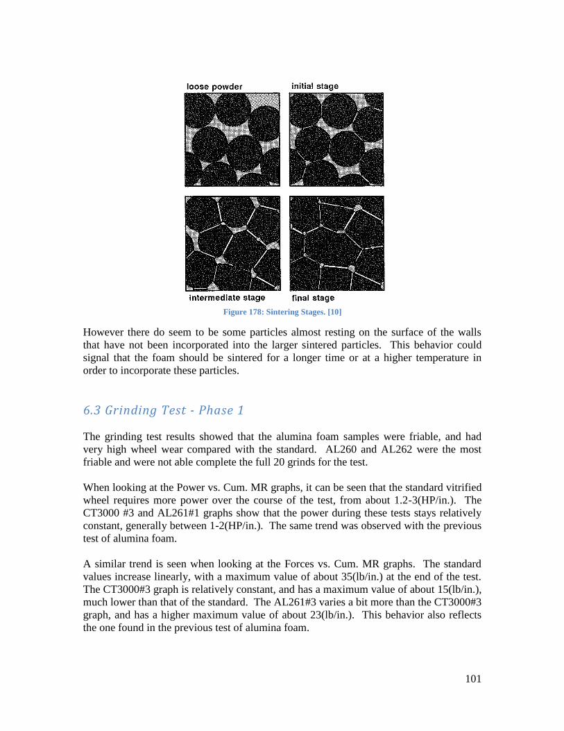
101

Figure 178: Sintering Stages. [10]

However there do seem to be some particles almost resting on the surface of the walls

that have not been incorporated into the larger sintered particles. This behavior could

signal that the foam should be sintered for a longer time or at a higher temperature in

order to incorporate these particles.

6.3 Grinding Test - Phase 1

The grinding test results showed that the alumina foam samples were friable, and had

very high wheel wear compared with the standard. AL260 and AL262 were the most

friable and were not able complete the full 20 grinds for the test.

When looking at the Power vs. Cum. MR graphs, it can be seen that the standard vitrified

wheel requires more power over the course of the test, from about 1.2-3(HP/in.). The

CT3000 #3 and AL261#1 graphs show that the power during these tests stays relatively

constant, generally between 1-2(HP/in.). The same trend was observed with the previous

test of alumina foam.

A similar trend is seen when looking at the Forces vs. Cum. MR graphs. The standard

values increase linearly, with a maximum value of about 35(lb/in.) at the end of the test.

The CT3000#3 graph is relatively constant, and has a maximum value of about 15(lb/in.),

much lower than that of the standard. The AL261#3 varies a bit more than the CT3000#3

graph, and has a higher maximum value of about 23(lb/in.). This behavior also reflects

the one found in the previous test of alumina foam.

102

The Surface Roughness and Surface Waviness vs. Cum. MR show that the standard

wheel had relatively low constant values (max 250 and 100µin), where CT3000 varied

slightly with higher values (max 300 and 230µin), and AL261 increased linearly with the

highest values (max 410 and 550µin). Surface finish is very important in I.D. grinding

and the alumina foam wheels should outperform the standard product.

There is a large variation between the two wheels tested from the same sample, especially

when focusing on the best performing alumina foam sample, CT3000. In terms of power,

the max value was 5(HP/in.) for #2 and barely 2(HP/in.) for #3. For the forces, the max

value for #2 seemed to be greater than 40(lb/in.), where as #3 had a max value of about

15(lb/in.). So in terms of power and forces, #3 seemed to perform the best. However, in

terms of surface roughness and waviness #2 seemed to perform better. For surface

roughness, #2 had a maximum value of 300µin and seemed fairly constant, where as #3

increased linearly to a maximum value of about 650µin. For surface waviness a similar

trend is seen, where #2 maximum value is about 330µin and #3 maximum value of

almost 400µin. This much variance between samples should not occur and in order to

create a dependable grinding product, this should be addressed.

An explanation for the wide variance in performance between the two CT3000 samples

could be due to the fact that there is a wide variation in porosity. CT3000#3 appears to

have a greater amount and size of porosity and performed better in terms of power and

forces. CT3000#2 had less porosity and smaller pore sizes, and performed better in terms

of surface roughness and waviness. Since surface finish is very important in I.D.

grinding a porosity close to that of CT3000#2 should be attained and able to be

repeatable.


All of the measured densities for the new alumina foam samples were close to the bulk

density values except for 356D. The 356D samples averaged a measured 1.57g/cc where

the bulk density was given as 1.46g/cc. This means that these samples would be less

porous than expected based on the bulk density.

For the porosity of the samples, all of them are about the same, with a range of 62-61.

However, the 356A and 356B have the lowest standard deviations with 0.3, and 356D not

far behind with 0.4. Based on this data 356C is the least reliable based on porosity and

should be expected to have the least reliable results in the grind test.

From the Grindo-sonic results, the 356A samples had the highest calculated Young‟s

Modulus with 55.82GPa, and 356D samples had the lowest with 49.72GPa. These values

are higher than the previous set of alumina foam samples, however these samples are also

much denser, at about 1.5g/cc as opposed to around 1g/cc for the previous samples. The

modulus is expected to be higher with a more dense sample. This trend can be seen

within the second sample set, where 356A has the highest bulk density, and 356D had the

lowest bulk density. The density of the foam is a function of sintering temperature, since

103

the higher the temperature the further the densification is allowed to take place because

the sintering process would occur faster. Based on the effects of an increased

temperature as discussed in Table 15 in Appendix II, 356A should exhibit:

- Greater shrinkage

- Grain growth

- Greater expense

- Less precision

- Higher properties

- Furnace limitations

- Pore coarsening

Basically the 356A samples should be the most dense with the highest properties, and the

356D samples should be the least dense and have the lowest properties.

The standard deviation from the Grindo-sonic test shows that 356A has the lowest

standard deviation with 0.58, and the 356B value is also relatively low at 1.44. The 356C

samples were much higher with a value of 6.03 and 356D samples were not far behind

with 5.11. This means that 356A would have the most consistent Young‟s Modulus, or

hardness. The 356A samples would be expected to perform more consistently in the

grinding test based on these results. It is interesting that so far 356A is exhibiting more

consistent properties than the other samples since it was mentioned that a higher sintering

temperature should result in less precision. However, the foam could possibly not go

through the full densification process, causing less shrinkage. Shrinkage during sintering

is somewhat uncontrollable and would result in less precision.


Looking at the CT Scan, the 356A and 356C samples have the largest range in pore size

of 100 - 3800µm. The ranges for the 356B and 356D samples are both about 100 -

2100µm. The scans show that the 356A sample has one large porosity, and the 356B and

356C samples have 2 large porosities each, all having an evenly distributed porosity

otherwise. The 356D sample seems to have a number of medium sized pores which are

distributed throughout the sample.

The porosity was also investigated through the SEM analysis, as well as the particle

sintering behavior. A wide range of macropores was observed, with 356A having the

largest range of about 80-765µm. The 356D samples appeared to have the smallest

macropore range of about 65-473µm. This could be due to the small sampling size, or

could be a function of sintering temperature. The interconnected pores seemed to be in

the same range for all of the samples, about 16-80µm. There also appeared to be more

interconnected pores in the 356C sample, however could be due to the small sample size.

There appear to be some larger particles inside the pores of the second phase samples, as

seen with the phase one sample AL262. There was a particle about 151µm found in

356B, which is comparable to the particle found in AL262. However, AL262 was made

104

from 50% 100µm particles, so this large size was expected. The 356B samples was made

from 100% 1µm particles, which means a large number of particles are sintering together,

or a piece of a wall possibly broke off and settled in the pore. The other particles found

in pores of the other phase two samples are on the order of 20µm, which would most

likely be particles sintering together.

All of the phase two samples had a similar structure looking at the pictures taken at

3000x. However, the 356A samples appeared to have more grain growth and the least

amount surface particles, where the 356D samples had the least grain growth and the

greatest amount of surface particles. This should be expected since 356A was sintered at

the highest temperature, 1700°C, and 356D at the lowest temperature, 1590°C.

Since there are still visible surface particles on 356A, this means the foam could be

sintered at an even higher temperature to eliminate them. However, the melting

temperature of alumina is 2323°C, and it has been found that the strength of sintered

alumina reaches a maximum at about 1800°C. [10] Also, an increase in sintering

temperature means an increase in the cost of manufacturing, so a higher sintering

temperature may not be desired and other factors may be altered.

6.6 Grinding Test – Phase 2

The purpose of the second grind test was to study the repeatability of the foam. If the

performance of the foam is repeatable, then it can be concluded that the porosity

throughout the sample is evenly distributed and controlled throughout.

From the power graphs it can be seen that the shape of the graph for 356A samples varies

from sample to sample, as do the graphs for 356B. The graphs for 356C are relatively the

same, and 356D has very similar graphs. However, the values for 356D increase rapidly,

where the values for 356A have the smallest increase. Based on these graphs 356D

appears to be the most consistent.

When comparing the forces, all of the graphs show similarity in their trend within each of

the samples. Although it should be noted that 356D again has rapidly increasing values,

and 356A has the lowest, and this trend can be observed in the surface finish graphs as

well.

Looking at the surface roughness, the graphs for 356A are somewhat similar, 356B and

356D vary between the different wheels. The samples from 356C produced similar

graphs and are the most consistent for surface roughness.

For surface waviness 356B and 356D were varied and their graphs showed no trend.

The graphs for 356C were varied and two of the three graphs showed no trend. The

graphs for 356A were similar and showed a trend, however one was slightly lower than

the rest. 356A was the most consistent in this category, and a lower value for surface

finish is more desirable, so the one graph that is slightly lower would not be an issue.

105

Based on the results from the second grind test it seems that various samples were more

consistent in different categories. The 356D samples were most consistent in terms of

power, the 356C samples were most consistent in terms of surface roughness, and the

356A were most consistent in terms of surface waviness. In terms of I.D. grinding,

surface finish is most important, so based the data from this grind test the 356A or 356C

samples would be the best.

Comparing the results from phase two with the results for the vitrified standard it can be

seen that 356A is the best performing sample. For the surface roughness, the vitrified

standard had values from 190-230µin and 0-50µin, where as 356A had values from 150-

210µin and 0-50µin. These values are basically the same for both samples and are

constant throughout the test. The surface waviness comparison showed similar results,

with values for both samples from 0-100µin, however the vitrified standard has slightly

lower values. In terms of surface finish, 356A is comparable to the vitrified standard.

However 356A had power and force values towards the high end of the vitrified standard

range, although these values were relatively constant throughout the test. In terms of

wheel wear the vitrified standard still outperforms the alumina foam, with a range of

0.0001 – 0.00015in compared with 0.0010 – 0.0015in for the foam. This is an

improvement over the phase one samples, but still an order of ten off from the vitrified

standard. Also, it should be noted that the wheels were not run in the rough grind test due

to high wheel wear. This means that the wheels are still too friable to be considered a

viable grinding wheel. Further improvements to the friability of the foam should be

made.

106

7.0 Conclusions

The first phase of samples focused on creating a more friable foam by varying the

particle size. Based on the results from the property evaluation and grinding test, the

following conclusions were made.

In terms of mechanical property testing, it can be concluded that the best way to calculate

the Young‟s Modulus is to use a Grindo-sonic test. The sample size that should be used

is 1x1/2x4in. bars in order to ensure consistent readings.

The SEM analysis showed that the larger particles tended to settle in the bottom of the

pores of the foam, which could be the only place they would fit since the pores are much

larger than the walls between the pores. The larger particles were also shown to

agglomerate towards the edge of a pore, but are mostly evenly dispersed. The analysis

also shows that a range of particle sizes can be found, however the sizes do not exceed

the largest particle size in the varied particle size samples. In the sample with 100% 1µm

particles, no more than three particles appear to be sintering together.

The CT Scan showed a variation in porosity size and distribution within the samples.

The variation was significant and affected the grinding performance of the samples.

From the grinding performance of the foams, an optimal friability was determined. The

samples that exhibited this friability were fabricated from 100% 1µm alumina particles.

However there was a large variation in grinding performance due to the variation in

porosity.

Based on the variation in grinding performance a second phase of samples were created

to control the porosity between samples by varying the temperature.

From the mechanical property evaluation of these samples, it was found that the density

calculation for one of the samples was significantly higher than the given bulk density,

signaling that the sample could have varied porosity. Based on the Grindo-sonic values,

one sample proved to be the most consistent in terms of Young‟s Modulus, or hardness.

The CT Scan showed that most of the samples have small, evenly dispersed porosity with

a few random large pores. However one sample had more medium porosity that was

evenly dispersed throughout the sample. This means that the sample was expected to

perform more consistently in terms of grinding performance.

From the SEM analysis, it appears that large amounts of particles are sintering together,

around 20µm. A larger particle was found, around 151µm, which could be particles

sintering together, or a broken piece of a wall. It also appears that the foam could be

sintered at a higher temperature, 1800°C, to reach the strength maximum of sintered

alumina and decrease the friability of the foam.

107

From the results of the second grind test, various samples performed more consistently in

different areas. However in terms of surface finish two samples performed the best,

although one of these was not the sample that appeared to have the most consistent

porosity based on the CT Scan.

Based on all of the results for the second phase of samples, an optimum sintering

temperature was chosen based on the grinding performance in terms of surface finish, as

well as the repeatability of the mechanical properties. The sintering temperature chosen

was 1700°C.

From all of the tests performed, an optimum friability and sintering temperature was

chosen. Theoretically if a sample were made with this friability and sintering

temperature it should outperform the current vitrified standard. However there are still

some investigations that could be done regarding the alumina foam.

108

8.0 Suggestions for Future Work

This thesis has investigated several areas with the alumina foam with regards to friability

and porosity control. Based on this research there are a few suggestions for future work.

First, a friability between that of the CT3000 samples and the previous alumina foam

samples is required. The CT3000 samples were made of 100% 1µm alumina particles,

and the previous alumina foam samples were made of 50% 1µm alumina particles and

50% tabular alumina. Since a friability between the two would be desired, a formulation

of 75% 1µm alumina particles and 25% tabular alumina sintered at 1700°C should be

tested.

Another suggestion would be to introduce secondary particles into the foam such as ZrO2,

MgO, or TiO2. The addition of these particles could improve the grinding performance

of the foam. The formulation including the secondary particles should be 50% 1µm

alumina and 50% 1µm secondary particle, sintered at the optimal temperature found

through this research of 1700°C.

A study to investigate the optimal density for the alumina foam could also be conducted.

Most of the densities chosen have been around 1g/cc, however the samples for the

porosity study were around 1.5g/cc. The wheels have performed well at 1g/cc, however a

full investigation might reveal that a wheel with different density would perform better.

Finally, the alumina foam could be expanded to different applications, such as super-

finishing. Super-finishing is a process that removes an outer layer of metal that has been

affected by high temperatures and pressures, leaving a stable material structure with low

tensile and compressive stresses. This process is typically used for shafts, rollers, and

bearings, and requires a very low surface finish at a low material removal rate. [15]

Alumina foam has excelled in this aspect, and would require little to no alteration to

begin testing in this application.

109

Appendices

Appendix I – Grinding

Grinding wheels have been used by manufacturers for over a hundred years. These self

sharpening wheels are important since they are capable of cutting, shaping, and finishing

products. The basic grinding wheel consists of abrasive grain, which cuts the work piece

material, and bond that holds the grain together in a matrix. Each component provides a

key role in the success of the grinding wheel. A general grinding wheel application can

be seen in Figure 179, showing all of the forces associated with this process.

Figure 179: Diagram of Basic Grinding. [16]

Vs = wheel speed

Vw = work speed

fv = cross slide speed

wv = rate of work radius change

sv = rate of wheel radius change

Kw = work support mechanism

Ks = wheel support system

K = wheel-work contact stiffness

Fn = force normal to contact surface

Ft = force tangential to contact surface

Both the work piece and the grinding wheel are decreasing in diameter, so a steady state

can be can be modeled by:

swf vvv (1) [16]

The abrasive grain is the component that does the most work interacting with the work

piece. There are three processes that occur between the grain and the work piece. First,

Rubbing occurs, creating elastic and/or plastic deformation in the work piece without

removing any material. Next, Ploughing causes plastic flow in the work piece in the

direction of sliding, creating a groove where extruded material has been thrown up and

110

broken off along the sides. This results in low rates of stock removal. Finally, Cutting

takes place when a fracture occurs in the plastically stressed zone just ahead of the

rubbing grain. This results in chip formation and high rates of stock removal. Cutting is

the desired process for grinding wheels, and a plot of Depth of Cut vs. Force Intensity in

Figure 180 shows the distinct region for this process. The graph also shows that there is a

certain Force Intensity that must be obtained in order to reach this region.

Figure 180: Wheel Depth of Cut vs. Force Intensity. [16]

Since in the grinding process both wheel and work piece are losing material, the material

removal rate (MRR) for each is of interest. These rates can be represented by the

following equations in cubic inches per minute:

Work piece: 60 www vWDZ (2) Dw = diameter of work piece

Wheel: 60 sss vWDZ (3) Ds = diameter of wheel

W = width of wheel-work contact [16]

There is a linear relationship between the material removal rate (MRR) and the normal

force in the cutting zone.

Work piece: Zw = Λw (Fn – Fno) (4) Λ = removal parameter (in3/min/lb)

Wheel: Zs = Λs Fn (5) Fno = threshold force [16]

The material removal parameters are further discussed later. The threshold force is the

force required to achieve metal removal, which is the force at the point where the cutting

zone begins. These equations show that as the normal force increases, the metal removal

rates increase. This increase in force has similar effects on surface finish and

horsepower, the higher the force the higher the surface finish values, resulting in a poorer

finish. Also, from Figure 181 it can be concluded that HP is represented by:

HP = 000,33

stVF

(6) [16]

111

And since Ft/Fn can be assumed to be a coefficient of friction, μ, the equation becomes:

HP = 000,33

snVF

(7) [16]

So as the normal force increases, the horsepower required increases. In Figure 181 the

relationship between metal and wheel removal rates and normal force is shown, as well

as the effect on surface finish and horsepower with removal parameters for a material

with Rockwell Hardness of 62.

Figure 181: Metal Removal Rate vs. Normal Force. [16]

The Λw, or metal removal parameter, is an important factor in grinding, and from

Equation 8 it can be seen that to increase MRR, Λw must be increased. It has been shown

that Λw is dependent on wheel speed, work piece hardness, dressing lead and depth.

These parameters can be used to calculate Λw.

112

Λw = 19/2738/547.0304/43

19/11

19/3

304/515

)()(

3

2

.021.0

ce

s

s

w

RdVolD

Vll

CL

V

V

lb

in

(in.

3/min, lb) (8) [16]

Λw = in.3/min, lb

Vw,Vs = work piece and wheel speeds (fpm)

L = dress lead (in/rev)

C = dress compensation (in. on diameter)

De = equivalent diameter (in.)

d = average grain size diameter (in.)

Vol = 1.33H + 2.2S – 8

Is the approximate volume percent of bond in wheel

Where wheel hardness is H, I, J, K, etc. and the value of H is 0, 1, 2, 3, etc. Also

S is the wheel structure number, such as 4, 6, etc.

This parameter can be increased by using a higher wheel speed, dressing lead, and

dressing ratio. Factors that cause this parameter to decrease are higher wheel-work

conformities, larger bond percentages in the grinding wheel and harder work pieces.

Figure 182: Metal Removal Parameter vs. Wheelspeed. [16]

113

Figure 182 shows Λw vs. Wheel speed, showing that increasing speed will increase the

metal removal parameter. The figure also shows the effect of hardness on Λw, where the

harder the material the lower the parameter.

Dressing, or sharpening, a grinding wheel also has an effect on Λw. The dressing lead

can be defined as

L = Table speed while dressing (in/sec)/ Wheel rotational speed (rev/sec) (9) [16]

The depth of dress measured on the diameter is represented by C, and the ratio of L

C

allows a comparison between different dresses. Figures 183 and 184 provide further

explanation of dressing values.

Figure 183: Diagram of Dressing. [16] Figure 184: Dressing Examples. [16]

The depth of dress can affect Λw, and in turn MRR, since it is changing the sharpness of

the wheel. This effect can be seen in Figure 185.

114

Figure 185: Affects of Dressing on Grinding Performance: Metal Removal Rate vs. Normal Force. [16]

From Figure 185 it is clear that by keeping a constant dress lead and increasing the depth

of dress, an increase in Λw occurred. A sharper wheel grinds more efficiently, therefore

increasing the MRR for a certain normal force.

Another factor in grinding is how well the grinding wheel conforms to the surface of the

work piece. This can be established by calculating the equivalent diameter, given by:

De = )/(1 ws

s

DD

D

Ds = wheel diameter Dw = work diameter (10) [16]

For an internal grinding operation, use a minus sign in the equation. For an external

grinding operation, use a plus sign. The better the wheel conforms to the work piece, the

higher the value of De. The effect of De on Λw is small on softer materials; however De

had a big impact on harder materials. These effects can be seen in Figure 186.

115

Figure 186: Effect of the Effective Diamater on Grinding Performance: Material Removal Rate v.s Force

Intensity. [16]

From the graph in Figure 186 it is observed that a higher De will result in a lower Λw.

This can be explained by the fact that when applying a constant feed rate during grinding,

force/inch force intensity is being applied at the wheel – work interface. This means the

larger the contact at the interface, the larger the force that is being applied while grinding.

This means that the rate at which the grinding wheel wears down is increased, and the

changes in the wheel diameter will in turn change the De, or conformity of the interface.

This change during grinding can result in a tapered work piece, so a small De that will

apply a small force at the interface, which decreases the rate that the grinding wheel

wears; creating less variation in the De during grinding is preferred.

Λs is dependent on many of the same variables as Λw, as well as wheel breakdown force

intensity.

Λs =

85.0/2.1

2 '

VolD

VFl

CllA

Vole

sn

(in.3/min, lb) (11) [16]

A = constant dependent upon coolant and grain type of wheel

'nF = force intensity (lbs/in.)

Vs = wheel speed (fpm)

l = dress lead (ipr)

C = dress compensation (in. on diameter)

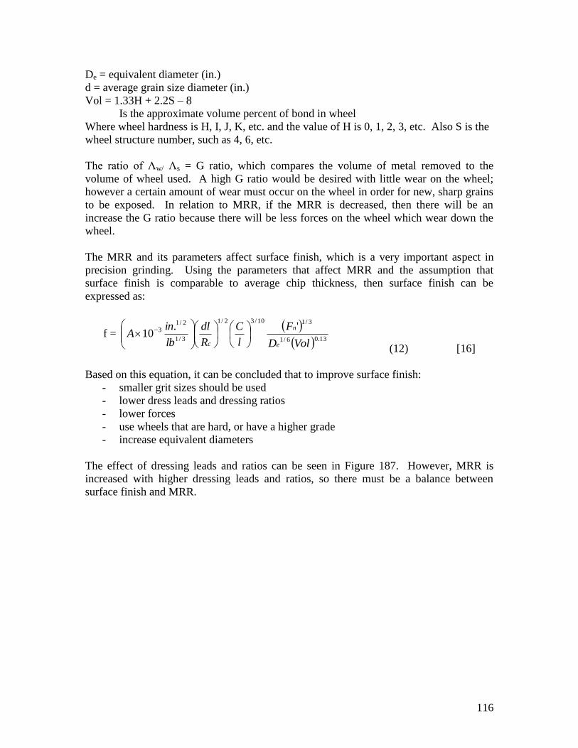
116

De = equivalent diameter (in.)

d = average grain size diameter (in.)

Vol = 1.33H + 2.2S – 8

Is the approximate volume percent of bond in wheel

Where wheel hardness is H, I, J, K, etc. and the value of H is 0, 1, 2, 3, etc. Also S is the

wheel structure number, such as 4, 6, etc.

The ratio of Λw/ Λs = G ratio, which compares the volume of metal removed to the

volume of wheel used. A high G ratio would be desired with little wear on the wheel;

however a certain amount of wear must occur on the wheel in order for new, sharp grains

to be exposed. In relation to MRR, if the MRR is decreased, then there will be an

increase the G ratio because there will be less forces on the wheel which wear down the

wheel.

The MRR and its parameters affect surface finish, which is a very important aspect in

precision grinding. Using the parameters that affect MRR and the assumption that

surface finish is comparable to average chip thickness, then surface finish can be

expressed as:

f =

13.06/1

3/110/32/1

3/1

2/13 '.

10VolD

F

l

C

R

dl

lb

inA

e

n

c

(12) [16]

Based on this equation, it can be concluded that to improve surface finish:

- smaller grit sizes should be used

- lower dress leads and dressing ratios

- lower forces

- use wheels that are hard, or have a higher grade

- increase equivalent diameters

The effect of dressing leads and ratios can be seen in Figure 187. However, MRR is

increased with higher dressing leads and ratios, so there must be a balance between

surface finish and MRR.

117

Figure 187: Surface Finish vs. Force Intensity. [16]

Surface finish compared with MRR at different wheel speeds can be seen Figure 188.

The graph shows that for a certain MRR, increasing the wheel speed will give a better

surface finish.

118

Figure 188: Surface Finish vs. Metal Removal Rate. [16]

Grinding is a balance between many parameters, and each application has a desired

outcome. In precision grinding, surface finish is very important and other parameters

may be sacrificed in order to achieve a good finish.

119

Appendix II - Sintering

Sintering is the process through which the particles are bonded together, or “the

consolidation, densification, recrystallization, and bonding obtained by heating

agglomerated powders during or following compaction, at temperatures below the

melting point of the principal component.” [10] The loose particles from milling are

mixed with additives, then compacted, and then heated at a certain temperature for a

certain amount of time. Typical sintering temperatures are high, such as 1400°C for

example, which is due to the high melting temperatures of ceramics. Alumina oxide has

a melting temperature of 2050°C, and can be sintered at 1600°C. In order to sinter a

ceramic at these temperatures, the ceramic must stay at these high temperatures for an

amount of time on the order of ten hours. Sintering is a complicated process and is

dependent on many different factors, the most obvious being time and temperature.

However, the surface tension and viscosity of the ceramic at the beginning of sintering

play a big role as well, and to control these parameters additives are used.

Additives produce the flow behavior and properties that are desired for forming. There

are many of these additives out there, and they can be broken down into several different

categories based on their functions. A liquid or a solvent medium would be added to

provide a viscous medium and dissolving agent. A surfactant, or wetting agent, would be

used to reduce surface and interfacial tension. This would improve wetting and

dispersion throughout the mixture. A deflocculant increases the repulsive forces between

particles to promote even dispersion. On the other hand, a coagulant is an electrolyte that

reduces the particle repulsion forces to promote agglomeration. A flocculant, or a binder,

will create a bridge between particles which allows it to act as a wetting aid, thickener,

suspension aid, rheological aid, body plasticizer, liquid retention agent, consistency aid,

or a binder. A plasticizer is used to modify viscoelastic properties. A lubricant is used to

reduce the resistance to sliding to improve surface smoothness and minimize adhesion

between surfaces. [17] One or many of these additives may be used in order to achieve

the desired sintering properties. Table 16 is a guide to how other factors can alter the

sintering process.

120

Table 16: Sintering Processing Effects. [10]

In order to fully understand sintering, the reactions between the particles during this

process must be understood. There are three basic stages of sintering, starting with neck

growth between adjacent particles, then material transport or densification, ending with

grain growth and elimination of isolated voids. [13] These are called the initial,

intermediate, and final stages of sintering. Each of these stages has certain geometric

stages that correspond. The initial stage has particles coming into contact with one

another to form a weak adhesive bond. A neck is rapidly formed with a small amount of

mass from the particles. In the intermediate stage, the pore structure becomes smooth

and develops interconnected pores that have a cylindrical shape. Sintering slows because

of a decrease in curvature and surface area. There is a possibility for grain growth at the

end of this stage. The final stage is when the pores collapse and pinch off to form

spherical pores. Densification also takes place during this stage. A summary of these

stages is in Table 17 and a pictorial representation in Figure 189.

121

Table 17: Geometric Stages of Sintering. [10]

Stage Microstructure

Initial - Neck size ratio (neck/particle) usually

less than 0.3

- Grain Size ~ Initial Size

- Surface area at least 50% of original

value

Intermediate - Density 70 – 92% of theoretical

- Grains become larger

- Pores are smoother

Final - Pores are closed

- Grain growth

- Total porosity < 8%

Figure 189: Stages of Sintering. [10]

122

Neck growth is an important aspect for sintering. This occurs when two particles come

into contact and mass transport takes place. The neck grows throughout the sintering

process and the larger the neck, the stronger the ceramic. If the neck is given enough

time to grow, the two particles will coalesce, creating a single particle that is larger than

the original particle size. These stages can be seen in Figure 191. Actual necking of

nickel spheres has been captured in a SEM picture, shown in Figure 190.

Figure 190: SEM pictures of Necking. [10]

123

Figure 191: Necking Model. [10]

In order for necking to occur, mass transport must take place during sintering. There are

six of these mechanisms that have been used to model mass transport during sintering.

These mechanisms are as follows: surface diffusion, grain boundary diffusion, plastic

flow, volume diffusion, viscous flow, and vapor transport.

Surface diffusion is a “motion of atoms between surface defects and is an initial

contributor in sintering of most materials.” [14] The surface defects that can be found on

an atom include ledges, kinks, vacancies, and adatoms. These defects can be seen in

figure 11. During diffusion, an atom will break away, typically at a kink, and will begin

to randomly move across the surface. The number of atoms that break away is dependent

on surface orientation and temperature. The atom will then reattach itself at an available

surface site. As sintering progresses, the significance of surface diffusion decreases,

however “it may play a role in affecting pore mobility during grain growth. Atomic

migration is from the low-curvature to the high-curvature regions on the pore surface

while it is being pulled by a moving grain boundary.” [10]

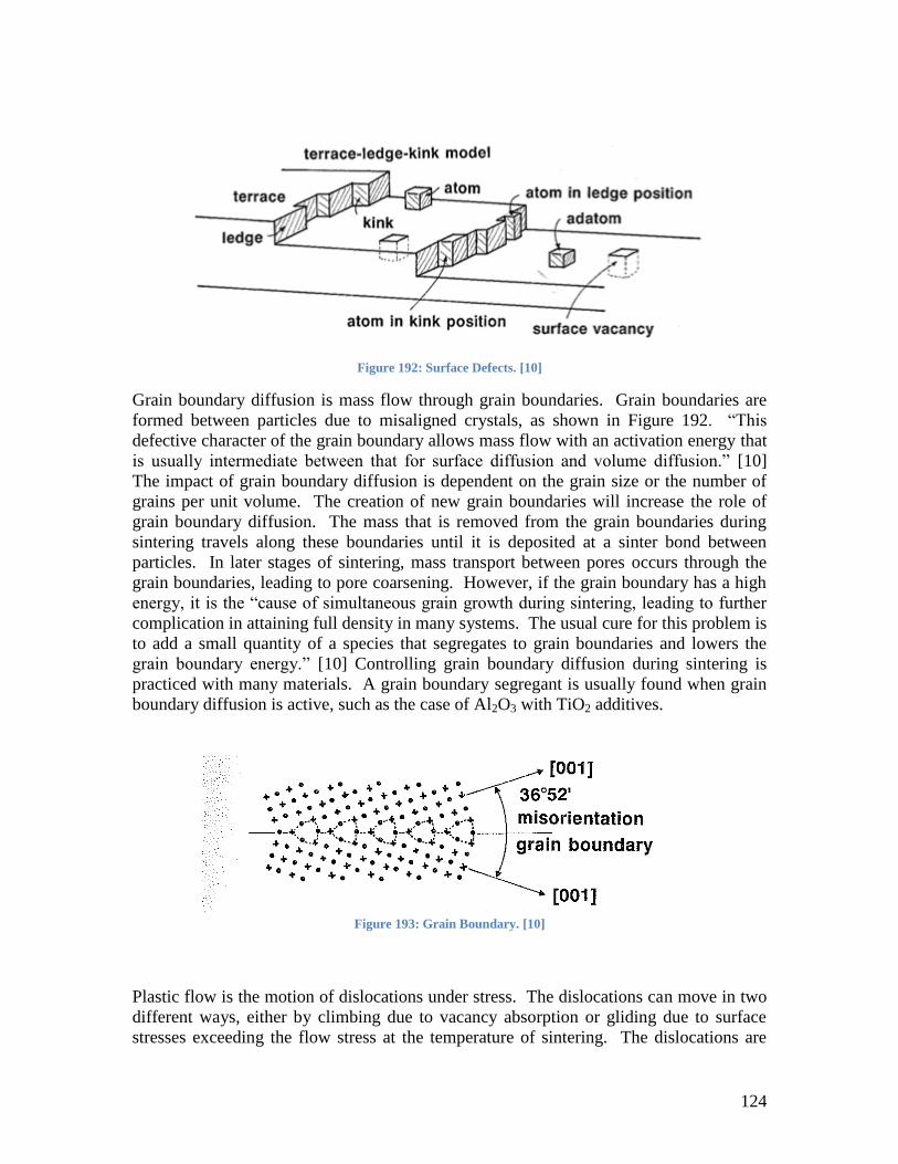
124

Figure 192: Surface Defects. [10]

Grain boundary diffusion is mass flow through grain boundaries. Grain boundaries are

formed between particles due to misaligned crystals, as shown in Figure 192. “This

defective character of the grain boundary allows mass flow with an activation energy that

is usually intermediate between that for surface diffusion and volume diffusion.” [10]

The impact of grain boundary diffusion is dependent on the grain size or the number of

grains per unit volume. The creation of new grain boundaries will increase the role of

grain boundary diffusion. The mass that is removed from the grain boundaries during

sintering travels along these boundaries until it is deposited at a sinter bond between

particles. In later stages of sintering, mass transport between pores occurs through the

grain boundaries, leading to pore coarsening. However, if the grain boundary has a high

energy, it is the “cause of simultaneous grain growth during sintering, leading to further

complication in attaining full density in many systems. The usual cure for this problem is

to add a small quantity of a species that segregates to grain boundaries and lowers the

grain boundary energy.” [10] Controlling grain boundary diffusion during sintering is

practiced with many materials. A grain boundary segregant is usually found when grain

boundary diffusion is active, such as the case of Al2O3 with TiO2 additives.

Figure 193: Grain Boundary. [10]

Plastic flow is the motion of dislocations under stress. The dislocations can move in two

different ways, either by climbing due to vacancy absorption or gliding due to surface

stresses exceeding the flow stress at the temperature of sintering. The dislocations are

125

able to climb due to “the absorption of vacancies emitted from the pores, leading to the

annihilation of the vacancies and dislocation motion to a new slip plane.” [10] This leads

to an improvement in mass transport, however this process causes the elimination of

dislocations, which leads to the termination of this process. Dislocation climb can also

improve densification rates, which can be modeled based on the rate of pore elimination

as shown in Equation 13.

2kTL

D

dt

dV VeP

(13) [10]

Where VP is the fractional volume of porosity, t is the time, σe is the effective surface

stress, Ω is the atomic volume, DV is the volume diffusion coefficient, k is Boltzmann‟s

constant, T is the absolute temperature, and L is the mean distance between mobile

dislocations. Plastic flow is more important during the beginning stages of sintering

when compaction and thermal stresses contribute to the overall stress of sintering. This

flow is favored by conditions when the heating rate is over 10°C/min, the particle size is

less than 100μm, or the sintering is pressure assisted. This type of flow has been

observed for Al2O3 when stress was applied during heating, however some scientists

disagree that plastic flow takes place during sintering.

Volume diffusion is the movement of vacancies through a crystalline structure. There are

three paths that the vacancies can take: through dislocations, free surfaces, or grain

boundaries. These can be seen in Figure 194. The rate at which these vacancies move is

dependent on temperature, composition, and curvature (or pressure).

Figure 194: Diffusion vacancy movement. [10]

The temperature determines the equilibrium number of vacancies; however the curvature

also has some effect. Because of this, mass flow into the neck region between particles

due to vacancy concentration difference in the microstructure. This vacancy

concentration, C, can be estimated by the curvature in Equation 14

126

21

111

RRkTCC o

(14) [10]

Where Co is the equilibrium vacancy concentration, γ is the surface energy, Ω is the

atomic volume, k is Boltzmann‟s constant, and T is the absolute temperature. This

vacancy concentration gradient in conjunction with a higher temperature creates vacancy

mobility, which leads to volume diffusion. The sintering rate due to volume diffusion

can be modeled using Fick‟s first law:

dx

dCDJ V (15) [10]

Where J is the flux in terms of atoms or vacancies per unit area per unit time, DV is the

diffusivity, and dC is the vacancy concentration change over a distance dx. In later stages

of the sintering process, pores can be thought of a collection of vacancies, unless there is

a gas trapped inside. If there are two adjacent pores that are different in size, the larger

pore will grow at the expense of the smaller pore, creating pore coarsening as show in

Figure 195. Volume diffusion is present in sintering of most materials; however the

activation energy for surface diffusion is usually the lowest, followed by grain boundary

diffusion.

Figure 195: Pore Coarsening. [10]

Viscous flow is observed when an amorphous material is under applied stress. An

amorphous material will show a decrease in viscosity as temperature increases. Sintering

puts stress on glass and polymer particles at high temperatures, and the lower the

viscosity of the material, the faster the sintering process. The viscosity of an amorphous

material can be represented by

kT

Qo exp (16) [10]

Where η is the viscosity, ηo is a proportionality coefficient, Q is the activation energy, k

is Boltzmann‟s constant, and T is the absolute temperature. The viscosity also plays a

role in neck size, as shown in Equation 17

127

D

t

D

X 32

(17) [10]

Where X is the neck diameter between particles with diameter D, γ is the surface energy,

and t is time. “As neck growth proceeds, amorphous materials can readily achieve a zero

curvature condition where the convex and concave radii are equal but opposite in sign.

This occurs at a neck size ratio of approximately X/D = 2/3 leading to greatly reduced

sintering near that point. As a practical consequence, low-packing-density structures can

not fully densify by viscous flow.” [9] The densification of a material based on viscosity

has been modeled as

D

t

V

V

Po

P

log (18) [18]

Where VP is the porosity after sintering and VPo is the initial porosity.

Vapor transport leads to the repositioning of atoms located on the particle surface without

densification. Evaporation and condensation occurs over pore space, and over time there

is a decrease in total surface area as bonds grow between particles. The equilibrium

vapor pressure, P, can be modeled using an Arrhenius equation

kT

QPP o exp (19) [10]

Where Po is a pre-exponential material constant, Q is the activation energy for

evaporation, k is Boltzmann‟s constant, and T is the absolute temperature. From this

dependence it can be determined that the higher the temperature, the higher the vapor

pressure, leading to an increase in vapor transport. During vapor transport, evaporation

usually takes place from flat or convex particles surfaces, and deposition at concave

necks between particles. In many instances vapor transport is slow, however small

powders with high surface areas and vapor pressures can be dominated by this transport.

Also, if a material is sintered in an atmosphere containing certain chemicals, then the role

of this transport is increased. When this occurs, then bonds can be created without

densification of the material, as shown in Figure 196.

128

Figure 196: Densification in different atmospheres. [10]

Figure 197: Dihedral Angle. [10]

The solid-vapor dihedral angle, , from Figure 197 is what dictates the neck growth. The

neck will grow until this angle reaches a force equilibrium with the surface and grain

boundary energies as shown in Equation 20.

2cos2

svss (20) [10]

Where γss is the grain boundary energy and γsv is the solid-vapor surface energy. The

grain size and neck size are also in balance as

2sin

GX (21) [10]

Where X is the neck size and G is the grain size. After the bond size ratio X/G as defined

by the dihedral angle is reached, then further neck growth is dependent on grain growth.

In the final stages of sintering, vapor transport contributes to pore motion, which is

modeled in Figure 198. “Mass evaporates from the lower curvature surface and deposits

on the higher curvature surface, giving an effective pore motion in the direction of the

129

moving grain boundary. Final stage densification is critically dependent on minimized

grain growth and attachment of the pores to grain boundaries.”

Figure 198: Grain Boundary Movement. [10]

During sintering there is a lot of stress present due to curved surfaces. The Laplace

equation models these stresses as

21

11

RR (22) [10]

Where σ is the stress associated with the curved surfaces, γ is the surface energy, and R1

and R2 are the principle radii of curvature for the surface, as shown in Figure 199.

Figure 199: Curved Particle. [10]

Convex surfaces have a positive value, meaning a tensile stress is present, and concave

surfaces have a negative value, indicating a compressive stress is present. A flat surface

will have no stress, so during sintering surfaces will try to flatten to decrease the amount

of stress.

130

When looking at two particles during sintering, the surface away from the neck has a

constant curvature, or R1=R2, and the Laplace equation can be re-written as

D

4 (23) [10]

where D is the diameter of the particle. For the stress due to the curvature at the neck, it

is assumed that the neck radius is circular and is labeled p, as shown in Figure 200. This

radius p can be approximated by X2/4D, and the stress becomes:

2

42

X

D

X (24) [10]

Figure 200: Particles Necking. [8]

There is a high stress gradient in the neck since there is a large change of curvature over a

small distance. This stress gradient provides a driving force for mass flow to the neck,

creating another mechanism for neck growth. As the neck grows the curvature flattens

out, the cylindrical pores then provide the driving force. In the final stage of sintering the

spherical pores drives shrinkage.

The pores and the grains in the final stage of sintering contribute to the sintering stress.

This can be modeled as

p

svss

dG

42 (25) [10]

where G is the grain size, γss is the grain boundary energy and γsv is the solid-vapor

surface energy, and dp is the pore size. Concave pores are given a negative sign, and

convex pores are given a positive sign.

Sintering stresses range from 0.05 to 60 MPa, largely depending on the pore size of the

material. Small pores and particles produce the highest stresses, which can lead to a

creep process. External stresses can also be applied during sintering, such as the case in

pressure-assisted sintering.

131

In summary, the basic stages of sintering are neck growth between adjacent particles,

material transport or densification, then grain growth with elimination of isolated voids.

These are also referred to as the initial, intermediate, and final stages of sintering. The

mechanism for sintering is mass transport, which can be defined with six diffusion and

transport mechanisms. They are surface diffusion, grain boundary diffusion, plastic flow,

volume diffusion, viscous flow, and vapor transport. During sintering stresses are

present, which are associated with curved surfaces, the neck radius, as well as pore and

grain size. There is also pressure-assisted sintering, which is when the material has a

stress applied during the sintering process. Sintering is an important process for the

ceramic materials we have today, and there is a lot of ongoing research into this subject

to create new materials for tomorrow.

132

Appendix III – Three-point Bend Test Data

CT3000:

Table 18: Data from Three-point bend test (CT3000).

Figure 201: Flexure Load vs. Flexure Extension - Three-point bend test (CT3000).

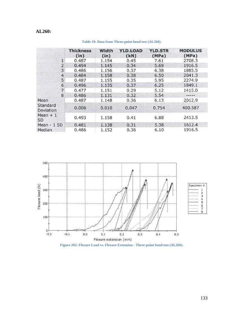
133

AL260:

Table 19: Data from Three-point bend test (AL260).

Figure 202: Flexure Load vs. Flexure Extension - Three-point bend test (AL260).

134

AL261:



135

AL262:



136

Bibliography

[1] Saint-Gobain. "Alumina Foam for Grinding." September 2007.

[2] Webster, M. Tricard and J. "Innovations in Abrasive Products for Precision Grinding." CIRP

Annals (2004).

[3] Gitzen, Walter H. Alumina as a Ceramic Material. The American Ceramic Society, 1970.

[4] Anne M. Bonner, Eric Bright, Edward L. Lambert, Dean S. Matsumoto, Xavier Orlhac, and

David A. Sheldon. Abrasive Articles with Novel Structures and Methods for Grinding. Unites

States of America: Patent US 7,275,980 B2. 2 October 2007.

[5] Ashby, Lorna J. Gibson and Michael F. Cellular Solids: Structure and Properties 2nd Ed. New

York: Cambridge University Press, 1997.

[6] James E. Dore, John C. Yarwood and Robert K. Preuss. Ceramic Foam and Method of

Preparation. Switzerland: Patent 4,024,212. 17 May 1977.

[7] Lee A. Carman, William S. Coblenz, and Janet L. Hammarstrom. Process of Producing Self-

Bonded Ceramic Abrasive Wheels. United States of America: Patent 5,221,294. 22 June 1993.

[8] David A. Sheldon, Carole J. Markhoff-Matheny, and Renato Terragni. High Porosity Vitrified

Bonded Grinding Wheels. United States of America: Patent 5,203,886. 20 April 1993.

[9] Jeevanantham, Muthu. Alumina Foam for Grinding - Bonded Abrasives. Status Report.

Worcester: Saint-Gobain, 2008.

[10] German, Randall M. Sintering Theory and Practice. New York: John Wiley & Sons, Inc., 1996.

[11] Barron, Rhonda L. Callender and Andrew R. "Chemical Control over Ceramic Porosity Using

Carboxylate-Alumoxane Nanoparticles." Advance Materials (2000): 734-8 Vol. 10.

[12] Boccaccini, Aldo R. Glass-Containing Composite Materials. Alternative Reinforcement

Concepts. London, UK: Imperial College London, n.d.

[13] Miao, Jianli Liu and Xigeng. "Porous alumina ceramics prepared by slurry infiltration of

expanded polystyrene beads." Journal of Materials Science (2005): 6145-50 Vol. 40.

[14] Frank J. T. Lin, Lutgard C. De Jonghe and Mohamed N. Rahaman. "Microstructure

Refinement of Sintered Alumina by a Two-Step Sintering Technique." Journal of the American

Ceramic Society (1997 ): 2269-77 Vol. 80.

137

[15] Dirk M. Shchibisch, Uwe Friedrich. Superfinishing Technology. Germany: Verlag Moderne

Industrie, 2006.

[16] Bhateja, Richard P. Lindsay and Chander P. Grinding: Theory, Techniques, and

Troubleshooting. Dearborn: Society of Manufacturing Engineers, 1982.

[17] Reed, James S. Introduction to the Principles of Ceramic Processing. New York: John Wiley

& Sons, 1988.

[18] Zagar, L. "Theoretical Aspects of Sintering Glass Powders." Sintering: New Developments

(1979): 57-64.

INVESTIGATION AND OPTIMIZATION OF A POROUS SINTERED ...

Documents

Transcript of INVESTIGATION AND OPTIMIZATION OF A POROUS SINTERED ...