
Introductory Geophysical Inverse Theory - Colorado School of Mines
208
Introductory Geophysical Inverse Theory John A. Scales, Martin L. Smith and Sven Treitel Samizdat Press
Transcript of Introductory Geophysical Inverse Theory - Colorado School of Mines

Introductory Geophysical Inverse Theory
John A. Scales, Martin L. Smith and Sven Treitel
SamizdatPress

2
Introductory Geophysical Inverse Theory
John A. Scales, Martin L. Smith and Sven Treitel
Samizdat Press Golden · White River Junction

3
Published by the Samizdat Press
Center for Wave PhenomenaDepartment of GeophysicsColorado School of MinesGolden, Colorado 80401
andNew England Research
76 Olcott DriveWhite River Junction, Vermont 05001
c©Samizdat Press, 2001
Samizdat Press publications are available via FTPfrom samizdat.mines.edu
Or via the WWW from http://samizdat.mines.eduPermission is given to freely copy these documents.

Contents
1 What Is Inverse Theory 1
1.1 Too many models . . . . . . . . . . . . . . . . . . . . . . . . . . . . . . 4
1.2 No unique answer . . . . . . . . . . . . . . . . . . . . . . . . . . . . . . 4
1.3 Implausible models . . . . . . . . . . . . . . . . . . . . . . . . . . . . . 5
1.4 Observations are noisy . . . . . . . . . . . . . . . . . . . . . . . . . . . 6
1.5 The beach is not a model . . . . . . . . . . . . . . . . . . . . . . . . . . 7
1.6 Summary . . . . . . . . . . . . . . . . . . . . . . . . . . . . . . . . . . 8
1.7 Beach Example . . . . . . . . . . . . . . . . . . . . . . . . . . . . . . . 8
2 A Simple Inverse Problem that Isn’t 11
2.1 A First Stab at ρ . . . . . . . . . . . . . . . . . . . . . . . . . . . . . . 12
2.1.1 Measuring Volume . . . . . . . . . . . . . . . . . . . . . . . . . 12
2.1.2 Measuring Mass . . . . . . . . . . . . . . . . . . . . . . . . . . . 12
2.1.3 Computing ρ . . . . . . . . . . . . . . . . . . . . . . . . . . . . 13
2.2 The Pernicious Effects of Errors . . . . . . . . . . . . . . . . . . . . . . 13
2.2.1 Errors in Mass Measurement . . . . . . . . . . . . . . . . . . . . 13
2.3 What is an Answer? . . . . . . . . . . . . . . . . . . . . . . . . . . . . 15
2.3.1 Conditional Probabilities . . . . . . . . . . . . . . . . . . . . . . 15
2.3.2 What We’re Really (Really) After . . . . . . . . . . . . . . . . . 16
2.3.3 A (Short) Tale of Two Experiments . . . . . . . . . . . . . . . . 16
ii CONTENTS
2.3.4 The Experiments Are Identical . . . . . . . . . . . . . . . . . . 17
2.4 What does it mean to condition on the truth? . . . . . . . . . . . . . . 20
2.4.1 Another example . . . . . . . . . . . . . . . . . . . . . . . . . . 21
3 Example: A Vertical Seismic Profile 25
3.0.2 Travel time fitting . . . . . . . . . . . . . . . . . . . . . . . . . 29
4 A Little Linear Algebra 33
4.1 Linear Vector Spaces . . . . . . . . . . . . . . . . . . . . . . . . . . . . 33
4.1.1 Matrices . . . . . . . . . . . . . . . . . . . . . . . . . . . . . . . 35
4.1.2 Matrices With Special Structure . . . . . . . . . . . . . . . . . . 38
4.2 Matrix and Vector Norms . . . . . . . . . . . . . . . . . . . . . . . . . 39
4.3 Projecting Vectors Onto Other Vectors . . . . . . . . . . . . . . . . . . 42
4.4 Linear Dependence and Independence . . . . . . . . . . . . . . . . . . . 45
4.5 The Four Fundamental Spaces . . . . . . . . . . . . . . . . . . . . . . . 46
4.5.1 Spaces associated with a linear system Ax = y . . . . . . . . . . 47
4.6 Matrix Inverses . . . . . . . . . . . . . . . . . . . . . . . . . . . . . . . 48
4.7 Eigenvalues and Eigenvectors . . . . . . . . . . . . . . . . . . . . . . . 49
4.8 Orthogonal decomposition of rectangular matrices . . . . . . . . . . . . 52
4.9 Orthogonal projections . . . . . . . . . . . . . . . . . . . . . . . . . . . 54
4.10 A few examples . . . . . . . . . . . . . . . . . . . . . . . . . . . . . . . 55
5 SVD and Resolution in Least Squares 59
5.0.1 A Worked Example . . . . . . . . . . . . . . . . . . . . . . . . . 59
5.0.2 The Generalized Inverse . . . . . . . . . . . . . . . . . . . . . . 61
5.0.3 Examples . . . . . . . . . . . . . . . . . . . . . . . . . . . . . . 66
5.0.4 Resolution . . . . . . . . . . . . . . . . . . . . . . . . . . . . . . 67

CONTENTS iii
6 A Summary of Probability and Statistics 71
6.1 Sets . . . . . . . . . . . . . . . . . . . . . . . . . . . . . . . . . . . . . 71
6.1.1 More on Sets . . . . . . . . . . . . . . . . . . . . . . . . . . . . 72
6.2 Random Variables . . . . . . . . . . . . . . . . . . . . . . . . . . . . . . 74
6.2.1 A Definition of Random . . . . . . . . . . . . . . . . . . . . . . 75
6.2.2 Generating random numbers on a computer . . . . . . . . . . . 75
6.3 Bayes’ Theorem . . . . . . . . . . . . . . . . . . . . . . . . . . . . . . . 78
6.4 Probability Functions and Densities . . . . . . . . . . . . . . . . . . . . 79
6.4.1 Expectation of a Function With Respect to a Probability Law . 82
6.4.2 Multi-variate probabilities . . . . . . . . . . . . . . . . . . . . . 83
6.5 Random Sequences . . . . . . . . . . . . . . . . . . . . . . . . . . . . . 86
6.5.1 The Central Limit Theorem . . . . . . . . . . . . . . . . . . . . 87
6.6 Expectations and Variances . . . . . . . . . . . . . . . . . . . . . . . . 89
6.7 Bias . . . . . . . . . . . . . . . . . . . . . . . . . . . . . . . . . . . . . 90
6.8 Correlation of Sequences . . . . . . . . . . . . . . . . . . . . . . . . . . 93
6.9 Random Fields . . . . . . . . . . . . . . . . . . . . . . . . . . . . . . . 96
6.10 Probabilistic Information About Earth Models . . . . . . . . . . . . . . 98
6.11 Other Common Analytic Distributions . . . . . . . . . . . . . . . . . . 101
6.12 Computer Exercise . . . . . . . . . . . . . . . . . . . . . . . . . . . . . 105
7 Linear Inverse Problems With Uncertain Data 107
7.0.1 Model Covariances . . . . . . . . . . . . . . . . . . . . . . . . . 109
7.1 The World’s Second Smallest Inverse Problem . . . . . . . . . . . . . . 109
7.1.1 The Damped Least Squares Problem . . . . . . . . . . . . . . . 112
8 Tomography 117
8.1 The X-ray Absorber . . . . . . . . . . . . . . . . . . . . . . . . . . . . 117

iv CONTENTS
8.1.1 The Forward Problem . . . . . . . . . . . . . . . . . . . . . . . 118
8.1.2 Linear Absorption . . . . . . . . . . . . . . . . . . . . . . . . . 119
8.1.3 Model Representation . . . . . . . . . . . . . . . . . . . . . . . 121
8.1.4 Some Numerical Results . . . . . . . . . . . . . . . . . . . . . . 122
8.2 Travel Time Tomography . . . . . . . . . . . . . . . . . . . . . . . . . . 124
8.3 Computer Example: Cross-well tomography . . . . . . . . . . . . . . . 125
9 From Bayes to Weighted Least Squares 131
10 Bayesian versus Frequentist Methods of Inference 135
10.0.1 Bayesian Inversion in Practice . . . . . . . . . . . . . . . . . . . 136
10.0.2 Bayes vs Frequentist . . . . . . . . . . . . . . . . . . . . . . . . 138
10.1 What Difference Does the Prior Make? . . . . . . . . . . . . . . . . . . 139
10.1.1 Bayes Risk . . . . . . . . . . . . . . . . . . . . . . . . . . . . . . 139
10.1.2 What is the Most Conservative Prior? . . . . . . . . . . . . . . 141
10.2 Example: A Toy Inverse Problem . . . . . . . . . . . . . . . . . . . . . 141
10.2.1 Bayes Risk . . . . . . . . . . . . . . . . . . . . . . . . . . . . . . 142
10.2.2 The Flat Prior is Informative . . . . . . . . . . . . . . . . . . . 142
10.3 Priors in High Dimensional Spaces: The Curse of Dimensionality . . . . 144
11 Iterative Linear Solvers 151
11.1 Classical Iterative Methods . . . . . . . . . . . . . . . . . . . . . . . . . 151
11.2 Conjugate Gradient . . . . . . . . . . . . . . . . . . . . . . . . . . . . . 154
11.2.1 Inner Products . . . . . . . . . . . . . . . . . . . . . . . . . . . 154
11.2.2 Quadratic Forms . . . . . . . . . . . . . . . . . . . . . . . . . . 154
11.2.3 Quadratic Minimization . . . . . . . . . . . . . . . . . . . . . . 155
11.2.4 Computer Exercise: Steepest Descent . . . . . . . . . . . . . . . 159
11.2.5 The Method of Conjugate Directions . . . . . . . . . . . . . . . 160

CONTENTS v
11.2.6 The Method of Conjugate Gradients . . . . . . . . . . . . . . . 162
11.2.7 Finite Precision Arithmetic . . . . . . . . . . . . . . . . . . . . 164
11.2.8 CG Methods for Least-Squares . . . . . . . . . . . . . . . . . . 166
11.2.9 Computer Exercise: Conjugate Gradient . . . . . . . . . . . . . 167
11.3 Practical Implementation . . . . . . . . . . . . . . . . . . . . . . . . . . 168
11.3.1 Sparse Matrix Data Structures . . . . . . . . . . . . . . . . . . . 168
11.3.2 Data and Parameter Weighting . . . . . . . . . . . . . . . . . . 169
11.3.3 Regularization . . . . . . . . . . . . . . . . . . . . . . . . . . . . 169
11.3.4 Jumping Versus Creeping . . . . . . . . . . . . . . . . . . . . . 171
11.3.5 How Smoothing Affects Jumping and Creeping . . . . . . . . . 172
11.4 Sparse SVD . . . . . . . . . . . . . . . . . . . . . . . . . . . . . . . . . 174
11.4.1 The Symmetric Eigenvalue Problem . . . . . . . . . . . . . . . . 174
11.4.2 Finite Precision Arithmetic . . . . . . . . . . . . . . . . . . . . 176
11.4.3 Explicit Calculation of the Pseudo-Inverse . . . . . . . . . . . . 179
12 More on the Resolution-Variance Tradeoff 183
12.1 A Surfer’s Guide to Backus-Gilbert Theory . . . . . . . . . . . . . . . . 183
12.2 Using the SVD . . . . . . . . . . . . . . . . . . . . . . . . . . . . . . . 185

vi CONTENTS
List of Figures
1.1 We think that gold is buried under the sand so we make measurementsof gravity at various locations on the surface. . . . . . . . . . . . . . . . 2
1.2 Inverse problems usually start with some procedure for predicting theresponse of a physical system with known parameters. Then we ask:how can we determine the unknown parameters from observed data? . 3
1.3 An idealized view of the beach. The surface is flat and the subsurfaceconsists of little blocks containing either sand or gold. . . . . . . . . . . 3
1.4 Our preconceptions as to the number of bricks buried in the sand. Thereis a possibility that someone has already dug up the gold, in which casethe number of gold blocks is zero. But we thing it’s most likely thatthere are 6 gold blocks. Possibly 7, but definitely not 3, for example.Since this preconception represents information we have independent ofthe gravity data, or prior to the measurements, it’s an example of whatis called a priori information. . . . . . . . . . . . . . . . . . . . . . . . . 5
1.5 Pirate chests were well made. And gold, being rather heavy, is unlikelyto move around much. So we think it’s mostly likely that the gold barsare clustered together. It’s not impossible that the bars have becomedispersed, but it seems unlikely. . . . . . . . . . . . . . . . . . . . . . . 6
1.6 The path connecting nature and the corrected observations is long anddifficult. . . . . . . . . . . . . . . . . . . . . . . . . . . . . . . . . . . . 7
1.7 The true distribution of gold bricks. . . . . . . . . . . . . . . . . . . . . 9
1.8 An unreasonable model that predicts the data. . . . . . . . . . . . . . . 10
2.1 A chunk of kryptonite. Unfortunately, kryptonite’s properties do notappear to be in the handbooks. . . . . . . . . . . . . . . . . . . . . . . 11
2.2 A pycnometer is a device that measures volumes via a calibrated beakerpartially filled with water. . . . . . . . . . . . . . . . . . . . . . . . . . 12
viii LIST OF FIGURES
2.3 A scale may or may not measure mass directly. In this case, it actuallymeasures the force of gravity on the mass. This is then used to infermass via Hooke’s law. . . . . . . . . . . . . . . . . . . . . . . . . . . . . 12
2.4 Pay careful attention to the content of this figure: It tells us the distri-bution of measurement outcomes for a particular true value. . . . . . . 14
2.5 Two apparently different experiments. . . . . . . . . . . . . . . . . . . 17
2.6 PT |O, the probability that the true density is x given some observed value. 18
2.7 A priori we know that the density of kryptonite cannot be less than 5.1or greater than 5.6. If we’re sure of this than we can reject any observeddensity outside of this region. . . . . . . . . . . . . . . . . . . . . . . . 20
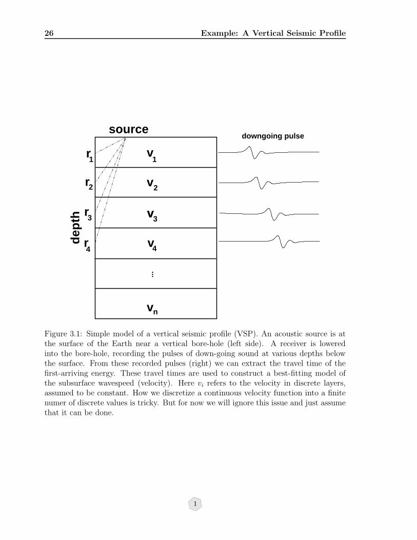
3.1 Simple model of a vertical seismic profile (VSP). An acoustic source is atthe surface of the Earth near a vertical bore-hole (left side). A receiver islowered into the bore-hole, recording the pulses of down-going sound atvarious depths below the surface. From these recorded pulses (right) wecan extract the travel time of the first-arriving energy. These travel timesare used to construct a best-fitting model of the subsurface wavespeed(velocity). Here vi refers to the velocity in discrete layers, assumed to beconstant. How we discretize a continuous velocity function into a finitenumer of discrete values is tricky. But for now we will ignore this issueand just assume that it can be done. . . . . . . . . . . . . . . . . . . . 26
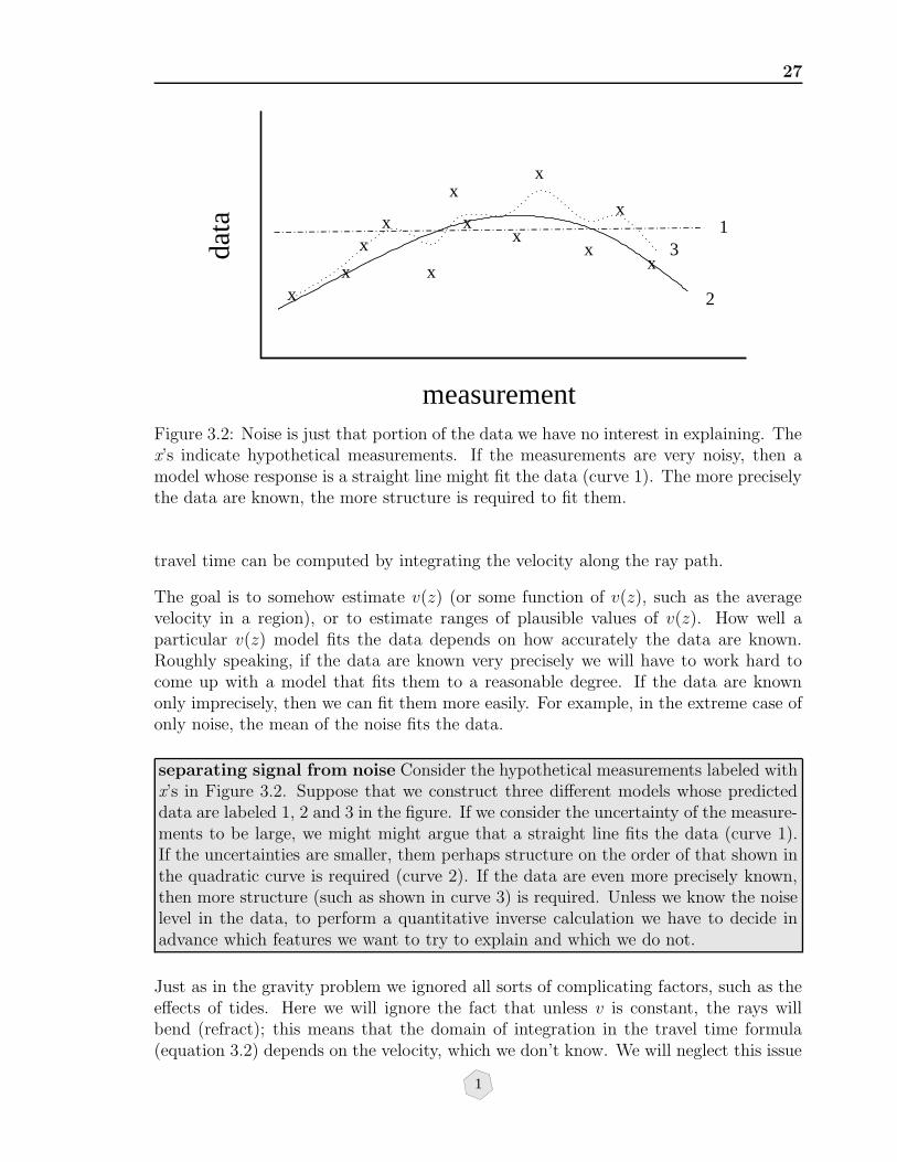
3.2 Noise is just that portion of the data we have no interest in explain-ing. The x’s indicate hypothetical measurements. If the measurementsare very noisy, then a model whose response is a straight line might fitthe data (curve 1). The more precisely the data are known, the morestructure is required to fit them. . . . . . . . . . . . . . . . . . . . . . . 27
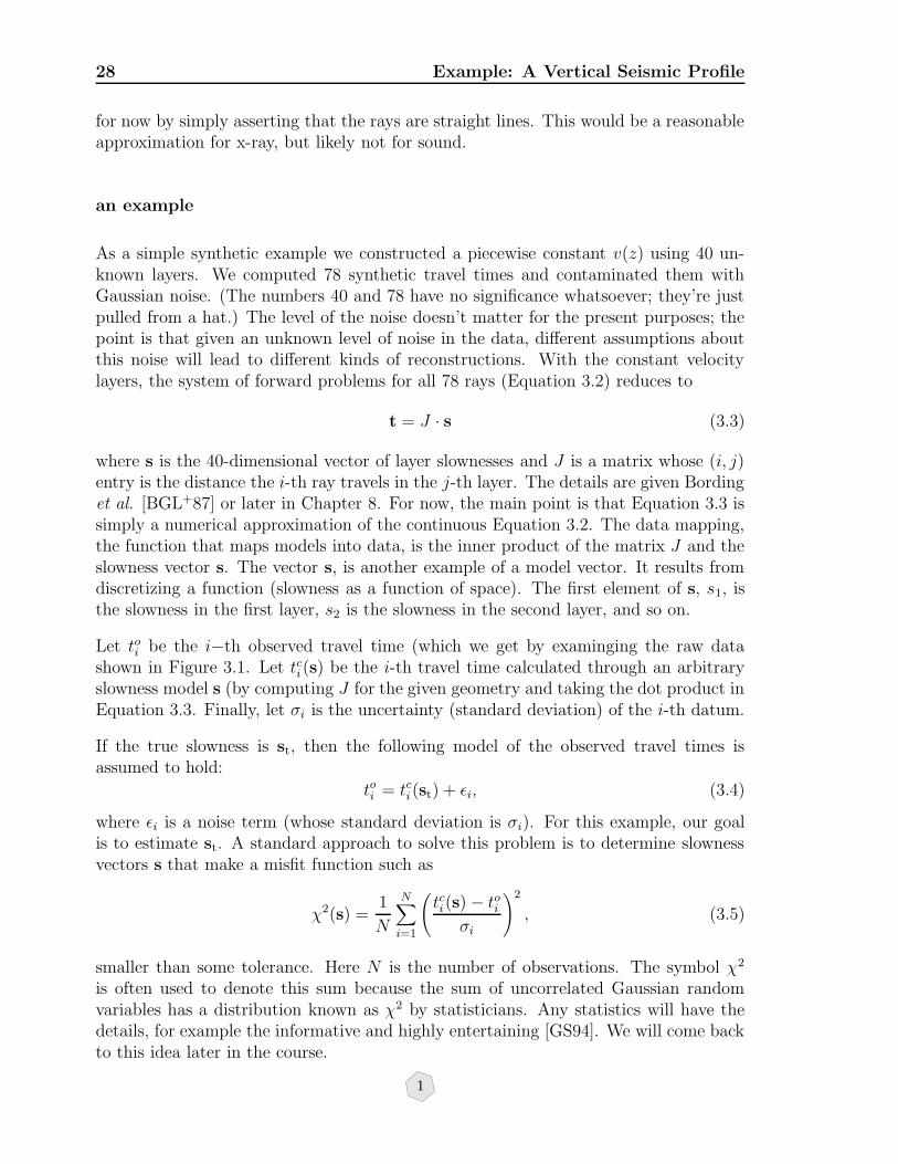
3.3 Observed data (solid curve) and predicted data for two different assumedlevels of noise. In the optimistic case (dashed curve) we assume the dataare accurate to 0.3 ms. In the more pessimistic case (dotted curve), weassume the data are accurate to only 1.0 ms. In both cases the predictedtravel times are computed for a model that just fits the data. In otherwords we perturb the model until the RMS misfit between the observedand predicted data is about N times 0.3 or 1.0, where N is the numberof observations. Here N = 78. I.e., Nχ2 = 78 × 1.0 for the pessimisticcase, and Nχ2 = 78× .3 for the optimistic case. . . . . . . . . . . . . . 30
LIST OF FIGURES ix
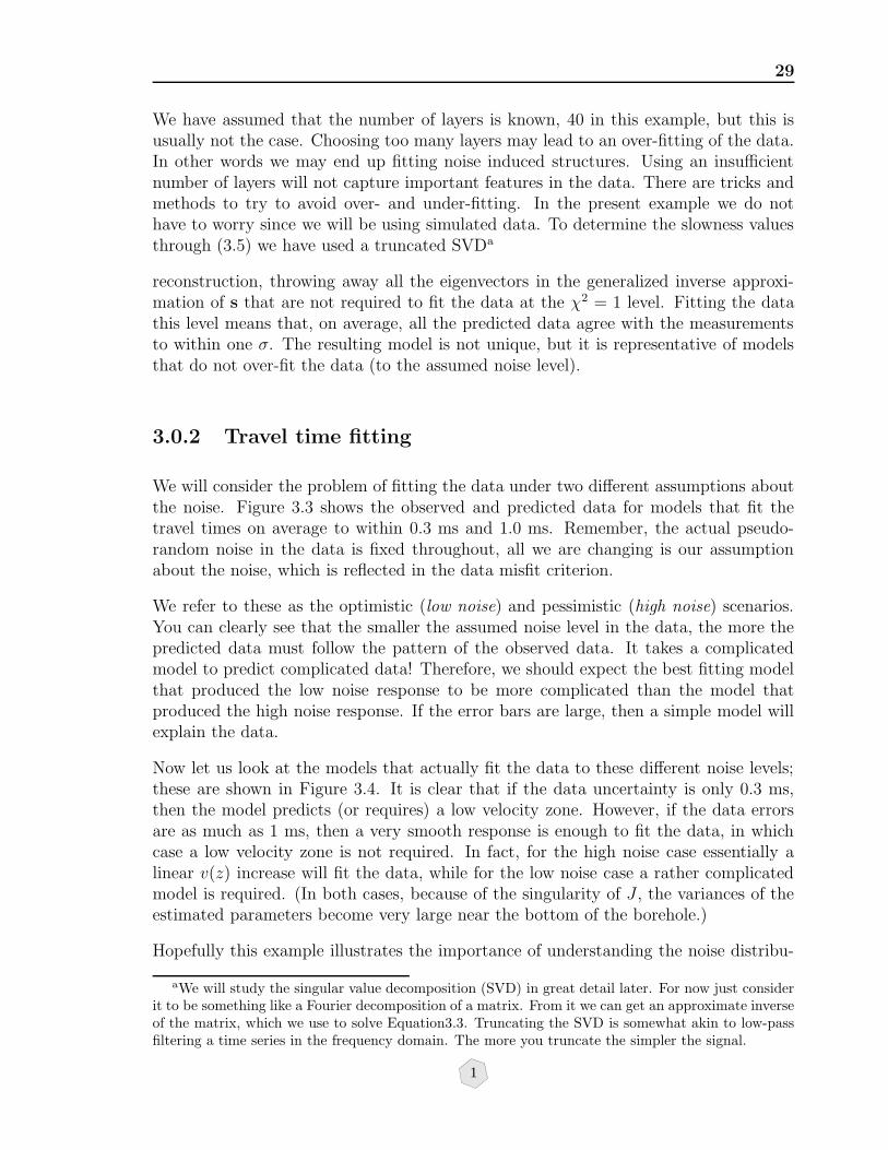
3.4 The true model (solid curve) and the models obtained by a truncatedSVD expansion for the two levels of noise, optimistic (0.3 ms, dashedcurve) and pessimistic (1.0 ms, dotted curve). Both of these models justfit the data in the sense that we eliminate as many singular vectors aspossible and still fit the data to within 1 standard deviation (normalizedχ2 = 1). An upper bound of 4 has also been imposed on the velocity.The data fit is calculated for the constrained model. . . . . . . . . . . . 31
4.1 Family of `p norm solutions to the optimization problem for various val-ues of the parameter λ. In accordance with the uniqueness theorem, wecan see that the solutions are indeed unique for all values of p > 1, butthat for p = 1 this breaks down at the point λ = 1. For λ = 1 there is acusp in the curve. . . . . . . . . . . . . . . . . . . . . . . . . . . . . . 41
4.2 Shape of the generalized Gaussian distribution for several values of p. . 43
4.3 Let a and b be any two vectors. We can always represent one, say b,in terms of its components parallel and perpendicular to the other. Thelength of the component of b along a is ‖b‖ cos θ which is also bTa/‖a‖. 44
6.1 Examples of the intersection, union, and complement of sets. . . . . . . 72
6.2 The title of Bayes’ article, published posthumously in the PhilosophicalTransactions of the Royal Society, Volume 53, pages 370–418, 1763 . . . 80
6.3 Bayes’ statement of the problem. . . . . . . . . . . . . . . . . . . . . . 80
6.4 A normal distribution of zero mean and unit variance. Almost all thearea under this curve is contained within 3 standard deviations of themean. . . . . . . . . . . . . . . . . . . . . . . . . . . . . . . . . . . . . 87
6.5 Ouput from the coin-flipping program. The histograms show the out-comes of a calculation simulating the repeated flipping of a fair coin.The histograms have been normalized by the number of trials, so whatwe are actually plotting is the relative probability of of flipping k headsout of 100. The central limit theorem guarantees that this curve has aGaussian shape, even though the underlying probability of the randomvariable is not Gaussian. . . . . . . . . . . . . . . . . . . . . . . . . . . 88
6.6 Two Gaussian sequences (top) with approximately the same mean, stan-dard deviation and 1D distributions, but which look very different. Inthe middle of this figure are shown the autocorrelations of these two se-quences. Question: suppose we took the samples in one of these timeseries and sorted them in order of size. Would this preserve the nicebell-shaped curve? . . . . . . . . . . . . . . . . . . . . . . . . . . . . . 94
x LIST OF FIGURES
6.7 38 realizations of an ultrasonic wave propagation experiment in a spa-tially random medium. Each trace is one realization of an unknownrandom process U(t). . . . . . . . . . . . . . . . . . . . . . . . . . . . . 97
6.8 A black box for generating pseudo-random Earth models that agree withour a priori information. . . . . . . . . . . . . . . . . . . . . . . . . . . 99
6.9 Three models of reflectivity as a function of depth which are consistentwith the information that the absolute value of the reflection coefficientmust be less than .1. On the right is shown the histogram of values foreach model. The top two models are uncorrelated, while the bottommodel has a correlation length of 15 samples. . . . . . . . . . . . . . . . 100
6.10 The lognormal is a prototype for asymmetrical distributions. It arisesnaturally when considering the product of a number of iid random vari-ables. This figure was generated from Equation 6.62 for s = 2. . . . . . 101
6.11 The generalized Gaussian family of distributions. . . . . . . . . . . . . 102
8.1 An x-ray source shoots x-rays across a target to a detector where theintensity (energy) of the beam is measured. . . . . . . . . . . . . . . . . 118
8.2 The fractional error of the linearized absorption as a function of ρexact. 120
8.3 Geometry of the tomography problem. The model is specified by blocksof constant absorption. . . . . . . . . . . . . . . . . . . . . . . . . . . . 121
8.4 A perspective view of the model. . . . . . . . . . . . . . . . . . . . . . 122
8.5 The model and shot geometry. . . . . . . . . . . . . . . . . . . . . . . . 123
8.6 . . . . . . . . . . . . . . . . . . . . . . . . . . . . . . . . . . . . . . . . 123
8.7 Plan view of the model showing one source and five receivers. . . . . . 124
8.8 Jacobian matrix for a cross hole tomography experiment involving 25×25rays and 20 × 20 cells (top). Black indicates zeros in the matrix andwhite nonzeros. Cell hit count (middle). White indicates a high totalray length per cell. The exact model used in the calculation (bottom).Starting with a model having a constant wavespeed of 1, the task is toimage the perturbation in the center. . . . . . . . . . . . . . . . . . . . 126
8.9 SVD reconstructed solutions. Using the first 10 singular values (top).Using the first 50 (middle). Using all the singular values above themachine precision (bottom). . . . . . . . . . . . . . . . . . . . . . . . . 128
LIST OF FIGURES xi
8.10 The distribution of singular values (top). A well resolved model singularvector (middle) and a poorly resolved singular vector (bottom). In thiscross well experiment, the rays travel from left to right across the figure.Thus, features which vary with depth are well resolved, while featureswhich vary with the horizontal distance are poorly resolved. . . . . . . 129
10.1 For square error loss, the Bayes risk associated with a uniform prioris shown along with the upper and lower bounds on the minimax riskas a function of the size of the bounding interval [−β, β]. When β iscomparable to or less than the variance (1 in this case), the risk associatedwith a uniform prior is optimistic . . . . . . . . . . . . . . . . . . . . . 143
11.1 Contours of the quadratic form associated with the linear system Ax =h where A = diag(10, 1) and h = (1,−1). Superposed on top of thecontours are the solution vectors for the first few iterations. . . . . . . . 159

xii LIST OF FIGURES

Chapter 1
What Is Inverse Theory
This course is an introduction to some of the balkanized family of techniques andphilosophies that reside under the umbrella of inverse theory. In this section we presentthe central threads that bind all of these singular items together in a harmonious whole.That’s impossible of course, but what we will do is provide a point of view that, while itwill break from time-to-time, is good enough to proceed with. The goal of this chapteris to introduce a real inverse problem and explore some of the issues that arise in anon-technical way. Later, we explore the resulting complications in greater depth.
Suppose that we find ourselves on a gleaming white beach somewhere in the Caribbeanwith
• time on our hands,
• a gravimeter (a little device that measures changes in gravitational acceleration),and
• the certain conviction that a golden blob of pirate booty lies somewhere beneathus.
In pursuit of wealth we make a series of measurements of gravity at several points alongthe surface. Our mental picture looks like Figure 1.1. And although we don’t knowwhere the gold actually is, or what amount is present, we’re pretty sure something isthere.
How can we use these observations to decide where the pirate gold lies and how muchis present? It’s not enough to know that gold (ρ = 19.3gm/cm3) is denser than sand(ρ = 2.2gm/cm3) and that the observed gravity should be greater above our futurewealth. Suppose that we observe relative gravity values of (from left to right)
22, 34, 30, 24, and 55µ gals
1

2 What Is Inverse Theory
x x
x x
Sand
Measurements
Surface
Figure 1.1: We think that gold is buried under the sand so we make measurements ofgravity at various locations on the surface.
respectively.a There’s no simple formula, (at least not that we know) into which we canplug five observed gravity observations and receive in return the depth and size of ourtarget.
So what shall we do? One thing we do know is
φ(r) =∫Gρ(r′)
|r− r′|dV′ (1.1)
that is, Newtonian gravitation. (If you didn’t know it before, you know it now.) Equa-tion 1.1 relates the gravitational potential, φ, to density, ρ. Equation 1.1 has twointeresting properties:
• it expresses something we think is true about the physics of a continuum, and
• it can be turned into an algorithm which we can apply to a given density field
So although we don’t know how to turn our gravity measurements into direct infor-mation about the density in the earth beneath us, we do know how to go in the otherdirection: given the density in the earth beneath us, we know how to predict the gravityfield we should observe. Inverse theory begins here, as in Figure 1.2.
For openers, we might write a computer program that accepts densities as inputs andproduces predicted gravity values as outputs. Once we have such a tool we can playwith different density values to see what kind of gravity observations we would get. Wemight assume that the gold is a rectangular block of the same dimensions as a standard
aA gal is a unit of acceleration equal to one centimeter per second per second. It is named afterGalileo but was first used in this century.
1

3
densitygravity
observed
densitypredicted
gravity
want:
have:
Figure 1.2: Inverse problems usually start with some procedure for predicting the re-sponse of a physical system with known parameters. Then we ask: how can we deter-mine the unknown parameters from observed data?
x x x x x
surface
sand
unknown
predictions
Figure 1.3: An idealized view of the beach. The surface is flat and the subsurfaceconsists of little blocks containing either sand or gold.
pirate’s chest and we could move the block to different locations, varying both depthand horizontal location, to see if we can match our gravity observations.
Part of writing the gravity program is defining the types of density models we’re goingto use. We’ll use a simplified model of the beach that has a perfectly flat surface,and has a subsurface that consists of a cluster of little rectangles of variable densitysurrounded by sand with a constant density. We’ve chosen the cluster of little rectanglesto include all of the likely locations of the buried treasure. (Did we mention we have amanuscript fragment which appears to be part of a pirate’s diary?) In order to modelhaving the buried treasure at a particular spot in the model we’ll set the density inthose rectangles to be equal to the density of gold and we’ll set the density in the restof the little rectangles to the density of sand. Here’s what the model looks like: The x’sare the locations for which we’ll compute the gravitational field. Notice that the valuesproduced by our program are referred to as predictions, rather than observations.
Now we have to get down to business and use our program to figure out where thetreasure is located. Suppose we embed our gravity program into a larger programwhich will
1
4 What Is Inverse Theory
• generate all possible models by trying all combinations of sand and gold densitiesin our little rectangles, and
• compare the predicted gravity values to the observed gravity values and tell uswhich models, if any, agreed well with the observations.
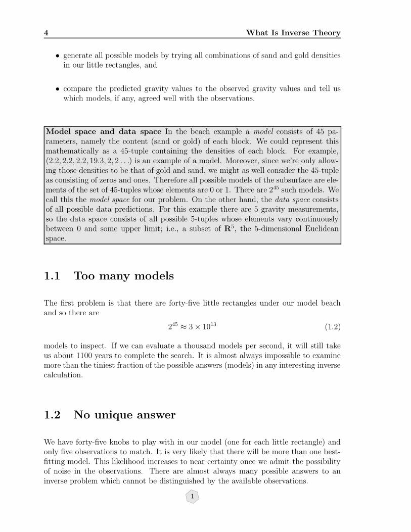
Model space and data space In the beach example a model consists of 45 pa-rameters, namely the content (sand or gold) of each block. We could represent thismathematically as a 45-tuple containing the densities of each block. For example,(2.2, 2.2, 2.2, 19.3, 2, 2 . . .) is an example of a model. Moreover, since we’re only allow-ing those densities to be that of gold and sand, we might as well consider the 45-tupleas consisting of zeros and ones. Therefore all possible models of the subsurface are ele-ments of the set of 45-tuples whose elements are 0 or 1. There are 245 such models. Wecall this the model space for our problem. On the other hand, the data space consistsof all possible data predictions. For this example there are 5 gravity measurements,so the data space consists of all possible 5-tuples whose elements vary continuouslybetween 0 and some upper limit; i.e., a subset of R5, the 5-dimensional Euclideanspace.
1.1 Too many models
The first problem is that there are forty-five little rectangles under our model beachand so there are
245 ≈ 3× 10¹³ (1.2)
models to inspect. If we can evaluate a thousand models per second, it will still takeus about 1100 years to complete the search. It is almost always impossible to examinemore than the tiniest fraction of the possible answers (models) in any interesting inversecalculation.
1.2 No unique answer
We have forty-five knobs to play with in our model (one for each little rectangle) andonly five observations to match. It is very likely that there will be more than one best-fitting model. This likelihood increases to near certainty once we admit the possibilityof noise in the observations. There are almost always many possible answers to aninverse problem which cannot be distinguished by the available observations.
1

1.3 Implausible models 5
someone elsefound it
it’s a little biggerthan we thought
relativelikelihood
0 1 2 3 4 5 6 7 8
number of gold rectangles in model
it’s all here
Figure 1.4: Our preconceptions as to the number of bricks buried in the sand. Thereis a possibility that someone has already dug up the gold, in which case the number ofgold blocks is zero. But we thing it’s most likely that there are 6 gold blocks. Possibly7, but definitely not 3, for example. Since this preconception represents information wehave independent of the gravity data, or prior to the measurements, it’s an example ofwhat is called a priori information.
1.3 Implausible models
On the basis of outside information (which we can’t reproduce here because we un-fortunately left it back at the hotel), we think that the total treasure was about theequivalent of six little rectangles worth of gold. We also think that it was buried in achest which is probably still intact (they really knew how to make pirate’s chests backthen). We can’t, however, be absolutely certain of either belief because storms couldhave rearranged the beach or broken the chest and scattered the gold about. It’s alsopossible that someone else has already found it. Based on this information we thinkthat some models are more likely to be correct than others. If we attach a relative like-lihood to different number of gold rectangles, our prejudices might look like Figure 1.4.You can imagine a single Olympic judge holding up a card as each model is displayed.
Similarly, since we think the chest is probably still intact we favor models which have allof the gold rectangles in the two-by-three arrangement typical of pirate chests, and wewill regard models with the gold spread widely as less likely. Qualitatively, our thoughtstend towards some specification of the relative likelihood of models, even before we’remade any observations, as illustrated in Figure 1.5. This distinction is hard to capturein a quasi-quantitative way.
1

6 What Is Inverse Theory
x x xx x x
x xx x x x
xx
x
xx
x
plausible
possible
unlikely
Figure 1.5: Pirate chests were well made. And gold, being rather heavy, is unlikelyto move around much. So we think it’s mostly likely that the gold bars are clusteredtogether. It’s not impossible that the bars have become dispersed, but it seems unlikely.
A priori information Information which is independent of the observations, such asthat models with the gold bars clustered are more likely than those in which the barsare dispersed, is called a priori information. We will continually make the distinctionbetween a priori (or simply prior, meaning before) and a posteriori (or simply posterior,meaning after) information. Posterior information is the result of the inferences wemake from data and the prior information.
What we’ve called plausibility really amounts to information about the subsurface thatis independent of the gravity observations. Here the information was historic and tookthe form of prejudices about how likely certain model configurations were with respectto one another. This information is independent of, and should be used in addition to,the gravity observations we have.
1.4 Observations are noisy
Most observations are subject to noise and gravity observations are particularly delicate.If we have two models that produce predicted values that lie within reasonable errorsof the observed values, we probably don’t want to put much emphasis on the possibilitythat one of the models may fit slightly better than the other. Clearly learning what theobservations have to tell us requires that we take account of noise in the observations.
1
1.5 The beach is not a model 7
Nature
(real beach)
real physics real gravity
observed gravity
transducer
(gravimeter)
corrections
for reality corrected
observed
gravity
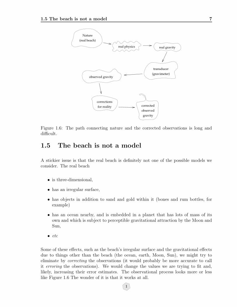
Figure 1.6: The path connecting nature and the corrected observations is long anddifficult.
1.5 The beach is not a model
A stickier issue is that the real beach is definitely not one of the possible models weconsider. The real beach
• is three-dimensional,
• has an irregular surface,
• has objects in addition to sand and gold within it (bones and rum bottles, forexample)
• has an ocean nearby, and is embedded in a planet that has lots of mass of itsown and which is subject to perceptible gravitational attraction by the Moon andSun,
• etc
Some of these effects, such as the beach’s irregular surface and the gravitational effectsdue to things other than the beach (the ocean, earth, Moon, Sun), we might try toeliminate by correcting the observations (it would probably be more accurate to callit erroring the observations). We would change the values we are trying to fit and,likely, increasing their error estimates. The observational process looks more or lesslike Figure 1.6 The wonder of it is that it works at all.
1
8 What Is Inverse Theory
Other effects, such as the three-dimensionality of reality, we might handle by alteringthe model to make each rectangle three-dimensional or by attaching modeling errors tothe predicted values.
1.6 Summary
Inverse theory is concerned with the problem of making inferences about physical sys-tems from data (usually remotely sensed). Since nearly all data are subject to someuncertainty, these inferences are usually statistical. Further, since one can only recordfinitely many (noisy) data and since physical systems are usually modeled by continuumequations, if there is a single model that fits the data there will be an infinity of them.To make these inferences quantitative one must answer three fundamental questions.How accurately are the data known? I.e., what does it mean to “fit” the data. Howaccurately can we model the response of the system? In other words, have we includedall the physics in the model that contribute significantly to the data. Finally, whatis known about the system independent of the data? Because for any sufficiently fineparameterization of a system there will be unreasonable models that fit the data too,there must be a systematic procedure for rejecting these unreasonable models.
1.7 Beach Example
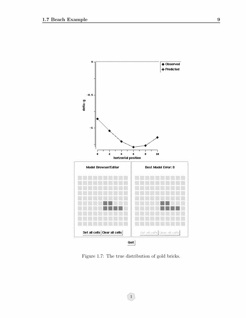
Here we show an example of the beach calculation. With the graphical user interfaceshown in Figure 1.7 we can fiddle with the locations of the gold/sand rectangles andvisually try to match the “observed” data. For this particular calculation, the truemodel has 6 buried gold bricks as shown in Figure 1.7. In Figure 1.8 we show but oneexample of a model that predicts the data essentially as well. The difference betweenthe observed and predicted data is not exactly zero, but given the noise that would bepresent in our measurements, it’s almost certainly good enough. So we see that twofundamentally different models predict the data about equally well.
1
1.7 Beach Example 9
Figure 1.7: The true distribution of gold bricks.
1

10 What Is Inverse Theory
Figure 1.8: An unreasonable model that predicts the data.
1

Chapter 2
A Simple Inverse Problem that Isn’t
Now we’re going to take a look at another inverse problem: estimating the density of thematerial in a body from information about the body’s weight and volume. Althoughthis sounds like a problem that is too simple to be of any interest to real inverters,we are going to show you that it is prey to exactly the same theoretical problems asan attempt to model the three-dimensional elastic structure of the earth from seismicobservations.
Here’s a piece of something (Figure 2.1): It’s green, moderately heavy, and it appearsto glow slightly (as indicated by the tastefully drawn rays in the figure). The chunkis actually a piece of kryptonite, one of the few materials for which physical propertiesare not available in handbooks. Our goal is to estimate the chunk’s density (which isjust the mass per unit volume). Density is just a scalar, such as 7.34, and we’ll use ρto denote various estimates of its value. Let’s use K to denote the chunk (so we don’thave to say chunk again and again).
Figure 2.1: A chunk of kryptonite. Unfortunately, kryptonite’s properties do not appearto be in the handbooks.
1

12 A Simple Inverse Problem that Isn’t
V
K
fluid level
Figure 2.2: A pycnometer is a device that measures volumes via a calibrated beakerpartially filled with water.
m = (kd)/gd
Figure 2.3: A scale may or may not measure mass directly. In this case, it actuallymeasures the force of gravity on the mass. This is then used to infer mass via Hooke’slaw.
2.1 A First Stab at ρ
In order to estimate the chunk’s density we need to learn its volume and its mass.
2.1.1 Measuring Volume
We measure volume with an instrument called a pycnometer. Our pycnometer consistsof a calibrated beaker partially filled with water. If we put K in the beaker, it sinks(which tells us right away that K is denser than water). If the fluid level in the beakeris high enough to completely cover K, and if we record the volume of fluid in the beakerwith and without K in it, then the difference in apparent fluid volume is equal to thevolume of K. Figure 2.2 shows a picture of everyman’s pycnometer. V denotes thechange in volume due to adding K to the beaker.
2.1.2 Measuring Mass
We seldom actually measure mass. What we usually measure is the force exerted onan object by the local gravitational field, that is, we put it on a scale and record theresultant force on the scale (Figure 2.3).
In this instance, we measure the force by measuring the compression of the spring hold-ing K up. We then convert that to mass by knowing (1) the local value of the Earth’sgravitational field, and (2) the (presumed linear) relation between spring extension and
1
2.2 The Pernicious Effects of Errors 13
force.
2.1.3 Computing ρ
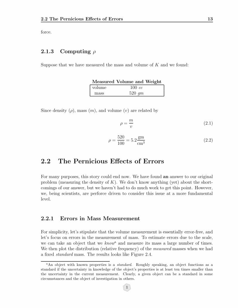
Suppose that we have measured the mass and volume of K and we found:
Measured Volume and Weightvolume 100 ccmass 520 gm
Since density (ρ), mass (m), and volume (v) are related by
ρ =m
v(2.1)
ρ =520
100= 5.2
gm
cm3(2.2)
2.2 The Pernicious Effects of Errors
For many purposes, this story could end now. We have found an answer to our originalproblem (measuring the density of K). We don’t know anything (yet) about the short-comings of our answer, but we haven’t had to do much work to get this point. However,we, being scientists, are perforce driven to consider this issue at a more fundamentallevel.
2.2.1 Errors in Mass Measurement
For simplicity, let’s stipulate that the volume measurement is essentially error-free, andlet’s focus on errors in the measurement of mass. To estimate errors due to the scale,we can take an object that we knowa and measure its mass a large number of times.We then plot the distribution (relative frequency) of the measured masses when we hada fixed standard mass. The results looks like Figure 2.4.
aAn object with known properties is a standard. Roughly speaking, an object functions as astandard if the uncertainty in knowledge of the object’s properties is at least ten times smaller thanthe uncertainty in the current measurement. Clearly, a given object can be a standard in somecircumstances and the object of investigation in others.
1

14 A Simple Inverse Problem that Isn’t
when the correct value is 5.2
probability of measuring x
probability of measuring 5.2
x5.2 5.4
probability of measuring 5.4
p(x)
Figure 2.4: Pay careful attention to the content of this figure: It tells us the distributionof measurement outcomes for a particular true value.
Physics News Number 183 by Phillip F. Schewe Improved mass values fornine elements and for the neutron have been published by an MIT research team,opening possibilities for a truly fundamental definition of the kilogram as well asthe most precise direct test yet of Einstein’s equation E = mc2. The new massvalues, for elements such as hydrogen, deuterium, and oxygen-16, are 20-1000 timesmore accurate than previous ones, with uncertainties in the range of 100 parts pertrillion. To determine the masses, the MIT team, led by David Pritchard, traps singleions in electric and magnetic fields and obtains each ion’s mass-to-charge ratio bymeasuring its cyclotron frequency, the rate at which it circles about in the magneticfield. The trapped ions, in general, are charged molecules containing the atoms ofinterest, and from their measurements the researchers can extract values for individualatomic masses. One important atom in the MIT mass table is silicon-28. With thenew mass value and comparably accurate measurements of the density and the latticespacing of ultrapure Si-28, a new fundamental definition of the kilogram (replacing thekilogram artifact in Paris) could be possible. The MIT team also plans to participate ina test of E = mc2 by using its mass values of nitrogen-14, nitrogen-15, and a neutron.When N-14 and a neutron combine, the resulting N- 15 atom is not as heavy as thesum of its parts, because it converts some of its mass into energy by releasing gammarays. In an upcoming experiment in Grenoble, France there are plans to measure the”E” side of the equation by making highly accurate measurements of these gammarays. (F. DeFilippo et al, Physical Review Letters, 12 September.)
1
2.3 What is an Answer? 15
2.3 What is an Answer?
Let’s consider how we can use this information to refine the results of our experiment.Since we have an observation (namely 5.2) we’d like to know the probability that thetrue density has a particular value, say 5.4.
This is going to be a little tricky, and it’s going to lead us into some unusual topics.We need to proceed with caution, and for that we need to sort out some notation.
2.3.1 Conditional Probabilities
Let ρO be the value of density we compute after measuring the volume and mass of K;we will refer to ρO as the observed density. Let ρT be the actual value of K’s density;we will refer to ρT as the true density.b
Let PO|T (ρO, ρT ) denote the conditional probability that we would measure ρO if thetrue density was ρT . The quantity plotted above is PO|T (ρO, 5.2), the probability thatwe would observe ρO if the true density was 5.2.
A few observations
First, keep in mind that in general we don’t know what the true value of the densityis. But if we nonetheless made repeated measurements we would still be mappingout PO|T , only this time it would be PO|T (ρO, ρT ). And secondly, you’ll notice in thefigure above that the true value of the density does not lie exactly at the peak of ourdistribution of observations. This must be the result of some kind of systematic errorin the experiment. Perhaps the scale is biased; perhaps we’ve got a bad A/D converter;perhaps there was a steady breeze blowing in the window of the lab that day.
A distinction is usually made between modeling or theoretical errors and random errors.A good example of a modeling error, would be assuming that K were pure kryptonite,when in fact it is an alloy of kryptonite and titanium. So in this case our theory isslightly wrong. In fact, we normally think of random noise as being the small scalefluctuations which occur when a measurement is repeated. Unfortunately this distinc-tion is hard to maintain in practice. Few experiments are truly repeatable. So whenwe try to repeat it, we’re actually introducing small changes into the assumptions; aswe repeatedly pick up K and put it back down on the scale, perhaps little bits fleck off,or some perspiration from our hands sticks to the sample, or we disturb the balance ofthe scale slightly by touching it. An even better example would be the positions of thegravimeters in the buried treasure example. We need to know these to do the modeling.
bWe will later consider whether this definition must be made more precise, but for now we willavoid the issue.
1

16 A Simple Inverse Problem that Isn’t
But every time we pick up the gravimeter and put it back to repeat the observation,we misposition it slightly. Do we regard these mispositionings as noise or do we regardthem as actual model parameters that we wish to infer? Do we regard the wind blowingnear the trees during our seismic experiment as noise, or could we actually infer thespeed of the wind from the seismic data? In fact, recent work in meterology has shownhow microseismic noise (caused by waves at sea) can be used to make inferences aboutclimate.
As far as we can tell, the distinction between random errors and theoretical errors issomewhat arbitrary and up to us to decide on a case by case. What it boils down toare: what features are we really interested in? Noise consists of those features of thedata we have no intest in explaining. For more details see the commentary: What isNoise? [SS98].
2.3.2 What We’re Really (Really) After
What we want is PT |O(ρT , ρO), the probability that ρT has a particular value giventhat we have the observed value ρO. Because PT |O and PO|T appear to be relationsbetween the same quantities, and because they look symmetric, it’s tempting to makethe connection
PT |O(ρT , ρO) = PO|T (ρO, ρT ) ?
but unfortunately it’s not true.
What is the correct expression for PT |O? More important, how can we think our waythrough issues like this?
We’ll start with the last question. One fruitful way to think about these issues is interms of a simple, repeated experiment. Consider the quantity we already have: PO|T ,which we plotted earlier. It’s easy to imagine the process of repeatedly weighing a massand recording the results. If we did this, we could directly construct tables of PO|T .
2.3.3 A (Short) Tale of Two Experiments
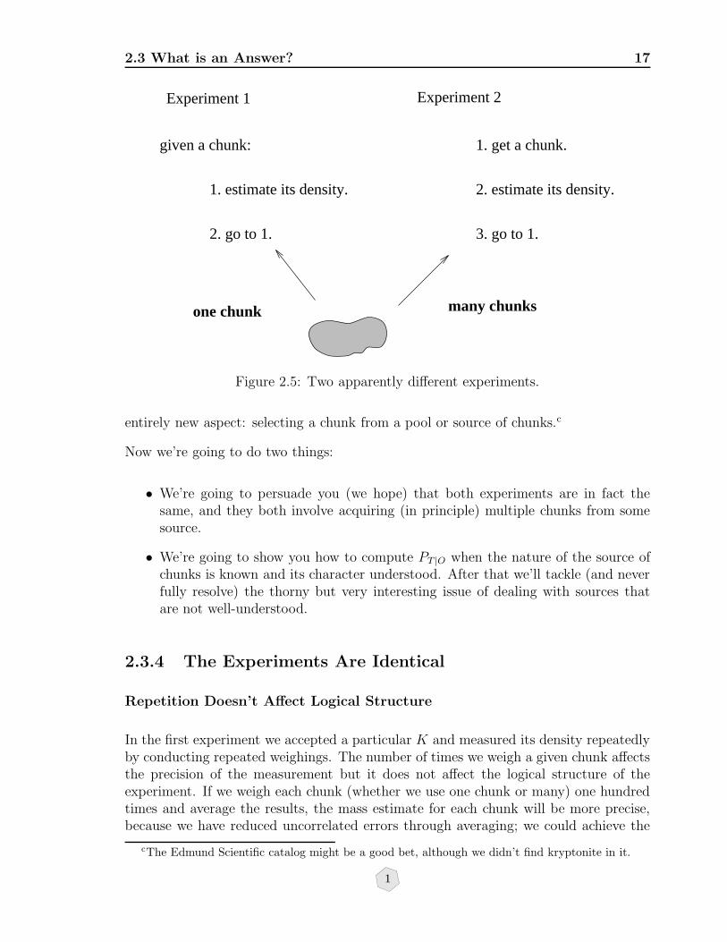
Now consider repeatedly estimating density. There are two ways we might think of this.In one experiment we repeatedly estimate the density of a particular, given chunk ofkryptonite. In the second experiment we repeatedly draw a chunk of kryptonite fromsome source and estimate its density.
These experiments appear to be quite different. The first experiment sounds just likethe measurements we (or someone) made to estimate errors in the scale, except in thiscase we don’t know the object’s mass to begin with. The second experiment has an
1
2.3 What is an Answer? 17
given a chunk:
1. estimate its density.
2. go to 1.
1. get a chunk.
2. estimate its density.
3. go to 1.
many chunksone chunk
Experiment 1 Experiment 2
Figure 2.5: Two apparently different experiments.
entirely new aspect: selecting a chunk from a pool or source of chunks.c
Now we’re going to do two things:
• We’re going to persuade you (we hope) that both experiments are in fact thesame, and they both involve acquiring (in principle) multiple chunks from somesource.
• We’re going to show you how to compute PT |O when the nature of the source ofchunks is known and its character understood. After that we’ll tackle (and neverfully resolve) the thorny but very interesting issue of dealing with sources thatare not well-understood.
2.3.4 The Experiments Are Identical
Repetition Doesn’t Affect Logical Structure
In the first experiment we accepted a particular K and measured its density repeatedlyby conducting repeated weighings. The number of times we weigh a given chunk affectsthe precision of the measurement but it does not affect the logical structure of theexperiment. If we weigh each chunk (whether we use one chunk or many) one hundredtimes and average the results, the mass estimate for each chunk will be more precise,because we have reduced uncorrelated errors through averaging; we could achieve the
cThe Edmund Scientific catalog might be a good bet, although we didn’t find kryptonite in it.
1

18 A Simple Inverse Problem that Isn’t
x5.2 5.4
p(x)
probability of a true density of x
when the observed value is 5.2
probability of true density of 5.2
probability of true density of 5.4
Figure 2.6: PT |O, the probability that the true density is x given some observed value.
same effect by using a correspondingly better scale. This issue is experimentally signif-icant but it is irrelevant to understanding the probabilistic structure of the experiment.For simplicity, then, we will assume that in both experiments, a particular chunk ismeasured only once.
Answer is Always a Distribution
In the (now slightly modified) first experiment, we are given a particular chunk, K, andwe make a single estimate of its mass, namely ρO. Since the scale is noisy, we have toexpress our knowledge of ρT , the true density, as a distribution showing the probabilitythat the true density has some value given that the observed density has some othervalue. Our first guess is that it might have the gaussianish form that we had for PO|TinFigure 2.4. So Figure 2.6 shows the suggested form for PT |O constructed by cloningthe earlier figure.
A Priori Pops Up
This looks pretty good until we consider whether or not we know anything about thedensity of kryptonite outside of the measurements we have made.
1
2.3 What is an Answer? 19
Suppose ρT is Known
Suppose that we know that the density of kryptonite is exactly
ρT = 1.7π
In that case, we must have
PT |O(ρT , ρO) = δ(ρT − 1.7π)
(where δ(x) is the Dirac delta-function) no matter what the observed value ρO is.
We are not asserting that the observed densities are all equal to 1.7π: the observationsare still subject to measurement noise. We do claim that the observations must alwaysbe consistent with the required value of ρT (or that some element of this theory iswrong). This shows clearly that PT |O 6= PO|T since one is a delta function, while theother must show the effects of experimental errors.
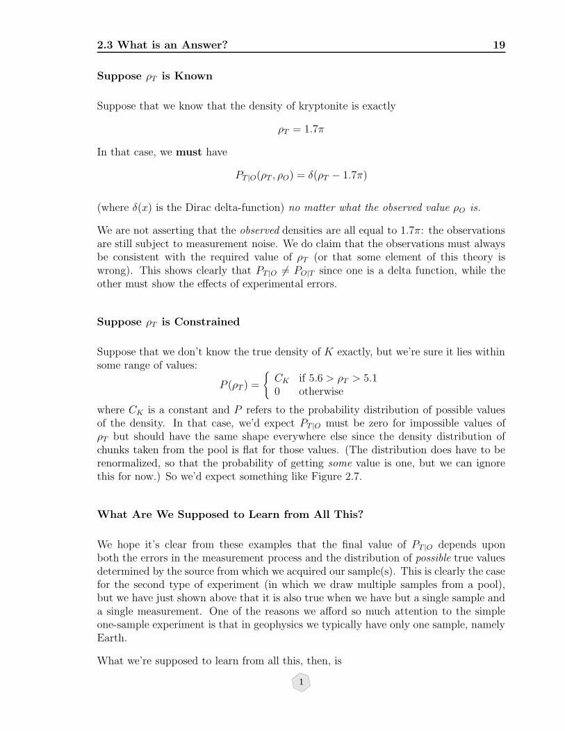
Suppose ρT is Constrained
Suppose that we don’t know the true density of K exactly, but we’re sure it lies withinsome range of values:
P (ρT ) =
CK if 5.6 > ρT > 5.10 otherwise
where CK is a constant and P refers to the probability distribution of possible valuesof the density. In that case, we’d expect PT |O must be zero for impossible values ofρT but should have the same shape everywhere else since the density distribution ofchunks taken from the pool is flat for those values. (The distribution does have to berenormalized, so that the probability of getting some value is one, but we can ignorethis for now.) So we’d expect something like Figure 2.7.
What Are We Supposed to Learn from All This?
We hope it’s clear from these examples that the final value of PT |O depends uponboth the errors in the measurement process and the distribution of possible true valuesdetermined by the source from which we acquired our sample(s). This is clearly the casefor the second type of experiment (in which we draw multiple samples from a pool),but we have just shown above that it is also true when we have but a single sample anda single measurement. One of the reasons we afford so much attention to the simpleone-sample experiment is that in geophysics we typically have only one sample, namelyEarth.
What we’re supposed to learn from all this, then, is
1
20 A Simple Inverse Problem that Isn’t
x =
0
5.65.4
5.65.4
Probability of a true density of x
when the observed value is 5.2
probability of a true density of 5.2
probability of a true density of 5.4
probability of a true density < 5.1 is zero
5.2
5.25.1
5.1
P(x)
x
CK
Figure 2.7: A priori we know that the density of kryptonite cannot be less than 5.1 orgreater than 5.6. If we’re sure of this than we can reject any observed density outsideof this region.
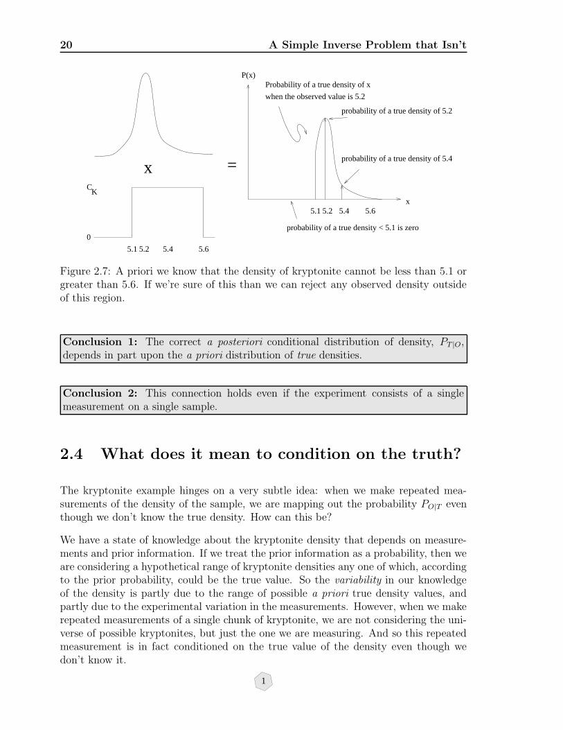
Conclusion 1: The correct a posteriori conditional distribution of density, PT |O,depends in part upon the a priori distribution of true densities.
Conclusion 2: This connection holds even if the experiment consists of a singlemeasurement on a single sample.
2.4 What does it mean to condition on the truth?
The kryptonite example hinges on a very subtle idea: when we make repeated mea-surements of the density of the sample, we are mapping out the probability PO|T eventhough we don’t know the true density. How can this be?
We have a state of knowledge about the kryptonite density that depends on measure-ments and prior information. If we treat the prior information as a probability, then weare considering a hypothetical range of kryptonite densities any one of which, accordingto the prior probability, could be the true value. So the variability in our knowledgeof the density is partly due to the range of possible a priori true density values, andpartly due to the experimental variation in the measurements. However, when we makerepeated measurements of a single chunk of kryptonite, we are not considering the uni-verse of possible kryptonites, but just the one we are measuring. And so this repeatedmeasurement is in fact conditioned on the true value of the density even though wedon’t know it.
1

2.4 What does it mean to condition on the truth? 21
Let us consider the simplest possible case, one observation, one parameter connectedby the forward problem:
d = m+ ε.
Assume that the prior distribution for m is N(0, β2) (the normal or Gaussian probabilitywith 0 mean and variance β2). Assume that the experimental error ε is N(0, σ2). Ifwe make repeated measurement of d on the same physical system (fixed m), then themeasurements will be centered about m (assuming no systematic errors) with variancejust due to the experimental errors, σ2. So we conclude that the probability (which wewill call f) of d given m is
f(d|m) = N(m, σ2). (2.3)
The definition of conditional probability is that
f(d,m) = f(d|m)f(m) (2.4)
where f(d,m) is the joint probability for model and data and f(m) is the probabilityon models independent of data; that’s our prior probability. So in this case the jointdistribution f(m, d) is
f(d,m) = N(m, σ2)×N(0, β2) ∝ exp[− 1
2σ2(d−m)2
]× exp
[− 1
2β2m2
]. (2.5)
So, if measuring the density repeatedly maps out f(d|m), then what is f(d)? We canget f(d) formally by just integrating f(d,m) over all m:
f(d) ≡∫f(d,m)dm =
∫ ∞
−∞exp
[− 1
2σ2(d−m)2
]× exp
[− 1
2β2m2
]dm.
This is the definition of a marginal probability. But now you can see that the variationsin f(d) depend on the a priori variations in m—we’re integrating over the universe ofpossible m values. This is definitely not what we do when we make a measurement.
2.4.1 Another example
Here is a more complicated example of the same idea, which we extend to the solutionof a toy “inverse” problem. It involves using n measurements and a normal prior toestimate a normal mean.
Assume that there are n observations d = (d1, d2, ...dn) which are iidd N(a, σ2) andthat we want to estimate the mean a given that the prior on a f(a) is N(µ, β2). Up toa constant factor, the joint distribution for a and d is:
dThe term iid is used to denote independent, identically distributed random variables. This meansthat the random variables are statistically independent of one another and they all have the sameprobability law.
1
22 A Simple Inverse Problem that Isn’t
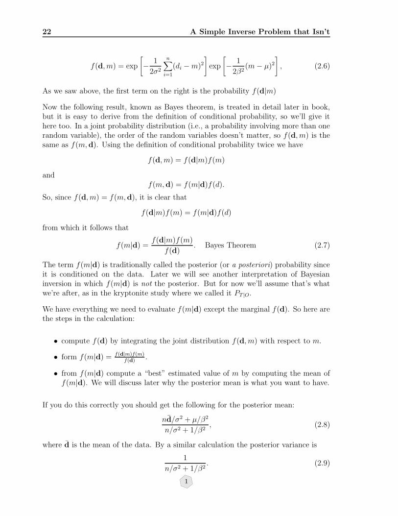
f(d, m) = exp
[− 1
2σ2
n∑
i=1
(di −m)2
]exp
[− 1
2β2(m− µ)2
], (2.6)
As we saw above, the first term on the right is the probability f(d|m)
Now the following result, known as Bayes theorem, is treated in detail later in book,but it is easy to derive from the definition of conditional probability, so we’ll give ithere too. In a joint probability distribution (i.e., a probability involving more than onerandom variable), the order of the random variables doesn’t matter, so f(d, m) is thesame as f(m,d). Using the definition of conditional probability twice we have
f(d, m) = f(d|m)f(m)
andf(m,d) = f(m|d)f(d).
So, since f(d, m) = f(m,d), it is clear that
f(d|m)f(m) = f(m|d)f(d)
from which it follows that
f(m|d) =f(d|m)f(m)
f(d). Bayes Theorem (2.7)
The term f(m|d) is traditionally called the posterior (or a posteriori) probability sinceit is conditioned on the data. Later we will see another interpretation of Bayesianinversion in which f(m|d) is not the posterior. But for now we’ll assume that’s whatwe’re after, as in the kryptonite study where we called it PT |O.
We have everything we need to evaluate f(m|d) except the marginal f(d). So here arethe steps in the calculation:
• compute f(d) by integrating the joint distribution f(d, m) with respect to m.
• form f(m|d) = f(d|m)f(m)f(d)
.
• from f(m|d) compute a “best” estimated value of m by computing the mean off(m|d). We will discuss later why the posterior mean is what you want to have.
If you do this correctly you should get the following for the posterior mean:
nd/σ2 + µ/β2
n/σ2 + 1/β2, (2.8)
where d is the mean of the data. By a similar calculation the posterior variance is
1
n/σ2 + 1/β2. (2.9)
1

BIBLIOGRAPHY 23
Notice that the posterior variance is always reduced by the presence of a nonzero β.The posterior mean can also be written as
[n/σ2
n/σ2 + 1/β2
]d +
[1/β2
n/σ2 + 1/β2
]µ.
Later we will see that the posterior mean has a special significance in that it minimizesa certain average error (called the risk). Because of this, the posterior mean has its ownname: it is called the Bayes estimator. In this example the Bayes estimator is a weightedaverage of the mean of the data and the mean of the Bayesian prior distribution; thelatter is the Bayes estimator before any data have been recorded.
Note also that as β → 0, increasingly strong prior information, the estimate convergesto the prior mean. As β →∞, increasingly weak prior information, the Bayes estimateconverges to the mean of the data.
Bibliography
[SS98] J.A. Scales and R. Snieder. What is noise? Geophysics, 63:1122–1124, 1998.
1

24 BIBLIOGRAPHY
1

Chapter 3
Example: A Vertical Seismic Profile
Here we will look at another simple example of a geophysical inverse calculation. Wewill cover the technical issues in due course. The goal here is simply to illustrate thefundamental role of data uncertainties in any inverse calculation. In this example wewill see that a certain model feature is near the limit of the resolution of the data.Depending on whether we are bold or conservative in assessing the errors of our data,this feature will or will not be required to fit the data.
We use a vertical seismic profile (VSP–used in exploration seismology to image theEarth’s near surface) experiment to illustrate how a fitted response depends on theassumed noise level in the data. Figure 3.1 shows the geometry of a VSP. A sourceof acoustic energy is at the surface near a vertical bore-hole (left side). A receiver islowered into a bore-hole, recording the travel time of the down-going acoustic pulse.These times are used to construct a “best-fitting” model of the wavespeed as a functionof depth v(z).
Of course the real velocity is a function of x, y, and z, but since in this example the rayspropagate almost vertically, there will be no point in trying ot resolve lateral variationsin v. If the Earth is not laterally invariant, this assumption introduces a systematicerror into the calculation.
For each observation (and hence each ray) the problem of data prediction boils downto computing the following integral:
t =∫
ray
1
v(z)d`. (3.1)
We can simplify the analysis somewhat by introducing the reciprocal velocity (calledslowness): s = 1/v. Now the travel time integral is linear in slowness:
t =∫
rays(z)d`. (3.2)
If the velocity model v(z) (or slowness s(z)) and the ray paths are known, then the
1
26 Example: A Vertical Seismic Profile
r
r
r
r
v
v
vv
v
1
2
3
n
downgoing pulse
4
3
2
1
source
dep
th
v4
...
Figure 3.1: Simple model of a vertical seismic profile (VSP). An acoustic source is atthe surface of the Earth near a vertical bore-hole (left side). A receiver is loweredinto the bore-hole, recording the pulses of down-going sound at various depths belowthe surface. From these recorded pulses (right) we can extract the travel time of thefirst-arriving energy. These travel times are used to construct a best-fitting model ofthe subsurface wavespeed (velocity). Here vi refers to the velocity in discrete layers,assumed to be constant. How we discretize a continuous velocity function into a finitenumer of discrete values is tricky. But for now we will ignore this issue and just assumethat it can be done.
1
27
xx
xx
x
x
x
x
x
x
x
x
1
2
3data
measurementFigure 3.2: Noise is just that portion of the data we have no interest in explaining. Thex’s indicate hypothetical measurements. If the measurements are very noisy, then amodel whose response is a straight line might fit the data (curve 1). The more preciselythe data are known, the more structure is required to fit them.
travel time can be computed by integrating the velocity along the ray path.
The goal is to somehow estimate v(z) (or some function of v(z), such as the averagevelocity in a region), or to estimate ranges of plausible values of v(z). How well aparticular v(z) model fits the data depends on how accurately the data are known.Roughly speaking, if the data are known very precisely we will have to work hard tocome up with a model that fits them to a reasonable degree. If the data are knownonly imprecisely, then we can fit them more easily. For example, in the extreme case ofonly noise, the mean of the noise fits the data.
separating signal from noise Consider the hypothetical measurements labeled withx’s in Figure 3.2. Suppose that we construct three different models whose predicteddata are labeled 1, 2 and 3 in the figure. If we consider the uncertainty of the measure-ments to be large, we might might argue that a straight line fits the data (curve 1).If the uncertainties are smaller, them perhaps structure on the order of that shown inthe quadratic curve is required (curve 2). If the data are even more precisely known,then more structure (such as shown in curve 3) is required. Unless we know the noiselevel in the data, to perform a quantitative inverse calculation we have to decide inadvance which features we want to try to explain and which we do not.
Just as in the gravity problem we ignored all sorts of complicating factors, such as theeffects of tides. Here we will ignore the fact that unless v is constant, the rays willbend (refract); this means that the domain of integration in the travel time formula(equation 3.2) depends on the velocity, which we don’t know. We will neglect this issue
1
28 Example: A Vertical Seismic Profile
for now by simply asserting that the rays are straight lines. This would be a reasonableapproximation for x-ray, but likely not for sound.
an example
As a simple synthetic example we constructed a piecewise constant v(z) using 40 un-known layers. We computed 78 synthetic travel times and contaminated them withGaussian noise. (The numbers 40 and 78 have no significance whatsoever; they’re justpulled from a hat.) The level of the noise doesn’t matter for the present purposes; thepoint is that given an unknown level of noise in the data, different assumptions aboutthis noise will lead to different kinds of reconstructions. With the constant velocitylayers, the system of forward problems for all 78 rays (Equation 3.2) reduces to
t = J · s (3.3)
where s is the 40-dimensional vector of layer slownesses and J is a matrix whose (i, j)entry is the distance the i-th ray travels in the j-th layer. The details are given Bordinget al. [BGL+87] or later in Chapter 8. For now, the main point is that Equation 3.3 issimply a numerical approximation of the continuous Equation 3.2. The data mapping,the function that maps models into data, is the inner product of the matrix J and theslowness vector s. The vector s, is another example of a model vector. It results fromdiscretizing a function (slowness as a function of space). The first element of s, s1, isthe slowness in the first layer, s2 is the slowness in the second layer, and so on.
Let toi be the i−th observed travel time (which we get by examinging the raw datashown in Figure 3.1. Let tci(s) be the i-th travel time calculated through an arbitraryslowness model s (by computing J for the given geometry and taking the dot product inEquation 3.3. Finally, let σi is the uncertainty (standard deviation) of the i-th datum.
If the true slowness is st, then the following model of the observed travel times isassumed to hold:
toi = tci(st) + εi, (3.4)
where εi is a noise term (whose standard deviation is σi). For this example, our goalis to estimate st. A standard approach to solve this problem is to determine slownessvectors s that make a misfit function such as
χ2(s) =1
N
N∑
i=1
(tci(s)− toi
σi
)2
, (3.5)
smaller than some tolerance. Here N is the number of observations. The symbol χ2
is often used to denote this sum because the sum of uncorrelated Gaussian randomvariables has a distribution known as χ2 by statisticians. Any statistics will have thedetails, for example the informative and highly entertaining [GS94]. We will come backto this idea later in the course.
1
29
We have assumed that the number of layers is known, 40 in this example, but this isusually not the case. Choosing too many layers may lead to an over-fitting of the data.In other words we may end up fitting noise induced structures. Using an insufficientnumber of layers will not capture important features in the data. There are tricks andmethods to try to avoid over- and under-fitting. In the present example we do nothave to worry since we will be using simulated data. To determine the slowness valuesthrough (3.5) we have used a truncated SVDa
reconstruction, throwing away all the eigenvectors in the generalized inverse approxi-mation of s that are not required to fit the data at the χ2 = 1 level. Fitting the datathis level means that, on average, all the predicted data agree with the measurementsto within one σ. The resulting model is not unique, but it is representative of modelsthat do not over-fit the data (to the assumed noise level).
3.0.2 Travel time fitting
We will consider the problem of fitting the data under two different assumptions aboutthe noise. Figure 3.3 shows the observed and predicted data for models that fit thetravel times on average to within 0.3 ms and 1.0 ms. Remember, the actual pseudo-random noise in the data is fixed throughout, all we are changing is our assumptionabout the noise, which is reflected in the data misfit criterion.
We refer to these as the optimistic (low noise) and pessimistic (high noise) scenarios.You can clearly see that the smaller the assumed noise level in the data, the more thepredicted data must follow the pattern of the observed data. It takes a complicatedmodel to predict complicated data! Therefore, we should expect the best fitting modelthat produced the low noise response to be more complicated than the model thatproduced the high noise response. If the error bars are large, then a simple model willexplain the data.
Now let us look at the models that actually fit the data to these different noise levels;these are shown in Figure 3.4. It is clear that if the data uncertainty is only 0.3 ms,then the model predicts (or requires) a low velocity zone. However, if the data errorsare as much as 1 ms, then a very smooth response is enough to fit the data, in whichcase a low velocity zone is not required. In fact, for the high noise case essentially alinear v(z) increase will fit the data, while for the low noise case a rather complicatedmodel is required. (In both cases, because of the singularity of J , the variances of theestimated parameters become very large near the bottom of the borehole.)
Hopefully this example illustrates the importance of understanding the noise distribu-
aWe will study the singular value decomposition (SVD) in great detail later. For now just considerit to be something like a Fourier decomposition of a matrix. From it we can get an approximate inverseof the matrix, which we use to solve Equation3.3. Truncating the SVD is somewhat akin to low-passfiltering a time series in the frequency domain. The more you truncate the simpler the signal.
1

30 Example: A Vertical Seismic Profile
0 10 20 30 40depth (m)
0
5
10
15
20
tim
e (m
s)
datahigh noise responselow noise response
Figure 3.3: Observed data (solid curve) and predicted data for two different assumedlevels of noise. In the optimistic case (dashed curve) we assume the data are accurateto 0.3 ms. In the more pessimistic case (dotted curve), we assume the data are accurateto only 1.0 ms. In both cases the predicted travel times are computed for a model thatjust fits the data. In other words we perturb the model until the RMS misfit betweenthe observed and predicted data is about N times 0.3 or 1.0, where N is the numberof observations. Here N = 78. I.e., Nχ2 = 78 × 1.0 for the pessimistic case, andNχ2 = 78× .3 for the optimistic case.
tion to properly interpret inversion estimates. In this particular case, we didn’t simplypull these standard deviations out of hat. The low value (0.3 ms) is what you happento get if you assume that the only uncertainties in the data are normally distributedfluctuations about the running mean of the travel times. However, keep in mind thatnature doesn’t really know about travel times. Travel times are approximations to thetrue properties (i.e., finite bandwidth) of waveforms. Further, the travel times them-selves are usually assigned by a human interpreter looking at the waveforms. Basedon these considerations, one might be led to conclude that a more reasonable estimateof the uncertainties for real data would be closer to 1 ms than 0.3 ms. In any event,the interpretation of the presence of a low velocity zone should be viewed with somescepticism unless the smaller uncertainty level can be justified.
1

31
0 10 20 30 40depth (m)
0
1
2
3
4
5
wav
e sp
eed
(m
/s)
true modelhigh noiselow noise
Figure 3.4: The true model (solid curve) and the models obtained by a truncated SVDexpansion for the two levels of noise, optimistic (0.3 ms, dashed curve) and pessimistic(1.0 ms, dotted curve). Both of these models just fit the data in the sense that weeliminate as many singular vectors as possible and still fit the data to within 1 standarddeviation (normalized χ2 = 1). An upper bound of 4 has also been imposed on thevelocity. The data fit is calculated for the constrained model.
1

32 BIBLIOGRAPHY
Bibliography
[BGL+87] R.P. Bording, A. Gersztenkorn, L.R. Lines, J.A. Scales, and S. Treitel. Ap-plications of seismic travel time tomography. Geophysical Journal of theRoyal Astronomical Society, 90:285–303, 1987.
[GS94] L. Gonick and W. Smith. Cartoon Guide to Statistics. HarperCollins, 1994.
1

Chapter 4
A Little Linear Algebra
Linear algebra background The parts of this chapter dealing with linear algebrafollow the outstanding book by Strang [Str88] closely. If this summary is too con-densed, you would be well advised to spend some time working your way throughStrang’s book. One difference to note however is that Strang’s matrices are m × n,whereas ours are n ×m. This is not a big deal, but it can be confusing. We’ll stickwith n×m because that is common in geophysics and later we will see that m is thenumber of model parameters in an inverse calculation.
4.1 Linear Vector Spaces
The only kind of mathematical spaces we will deal with in this course are linear vectorspaces. You are already well familiar with concrete examples of such spaces, at least inthe geometrical setting of vectors in three-dimensional space. We can add any two, say,force vectors and get another force vector. We can scale any such vector by a numericalquantity and still have a legitimate vector. However, in this course we will use vectorsto encapsulate discrete information about models and data. If we record one seismictrace, one second in length at a sample rate of 1000 samples per second, and let eachsample be defined by one byte, then we can put these 1000 bytes of information in a1000-tuple
(s1, s2, s3, · · · , s1000) (4.1)
where si is the i-th sample, and treat it just as we would a 3-component physical vector.That is, we can add any two such vectors together, scale them, and so on. When we“stack” seismic traces, we’re just adding these n-dimensional vectors component bycomponent, say trace s plus trace t,
s+ t = (s1 + t1, s2 + t2, s3 + t3, · · · , s1000 + t1000). (4.2)
0
34 A Little Linear Algebra
Now, the physical vectors have a life independent of the particular 3-tuple we use torepresent them. We will get a different 3-tuple depending on whether we use cartesianor spherical coordinates, for example; but the force vector itself is independent of theseconsiderations. On the other hand, our use of vector spaces is purely abstract. Thereis no physical seismogram vector; all we have is the n-tuple sampled from the recordedseismic trace.
Further, the mathematical definition of a vector space is sufficiently general to incor-porate objects that you might not consider as vectors at first glance–such as functionsand matrices. The definition of such a space actually requires two sets of objects: a setof vectors V and a one of scalars F . For our purposes the scalars will always be eitherthe real numbers R or the complex numbers C. For this definition we need the idea ofa Cartesian product of two sets.
Definition 1 Cartesian product The Cartesian product A×B of two sets A and Bis the set of all ordered pairs (a, b) where a ∈ A and b ∈ B.
Definition 2 Linear Vector Space A linear vector space over a set F of scalarsis a set of elements V together with a function called addition from V × V into Vand a function called scalar multiplication from F × V into V satisfying the followingconditions for all x, y, z ∈ V and all α, β ∈ F :
V1: (x + y) + z = x + (y + z)
V2: x + y = y + x
V3: There is an element 0 in V such that x + 0 = x for all x ∈ V .
V4: For each x ∈ V there is an element −x ∈ V such that x + (−x) = 0.
V5: α(x + y) = αx+ αy
V6: (α + β)x = αx + βx
V7: α(βx) = (αβ)x
V8: 1 · x = x
The simplest example of a vector space is Rn, whose vectors are n-tuples of real numbers.Addition and scalar multiplication are defined component-wise:
(x1, x2, · · · , xn) + (y1, y2, · · · , yn) = (x1 + y1, x2 + y2, · · · , xn + yn) (4.3)
andα(x1, x2, · · · , xn) = (αx1, αx2, · · · , αxn). (4.4)
0
4.1 Linear Vector Spaces 35
In the case of n = 1 the vector space V and the scalars F are the same. So trivially, Fis a vector space over F .
A few observations: first, by adding −x to both sides of x + y = x, you can show thatx+ y = x if and only if y = 0. This implies the uniqueness of the zero element and alsothat α · 0 = 0 for all scalars α.
Functions themselves can be vectors. Consider the space of functions mapping somenonempty set onto the scalars, with addition and multiplication defined by:
[f + g](t) = f(t) + g(t) (4.5)
and
[αf ](t) = αf(t). (4.6)
We use the square brackets to separate the function from its arguments. In this case,the zero element is the function whose value is zero everywhere. And the minus elementis inherited from the scalars: [−f ](t) = −f(t).
4.1.1 Matrices
The set of all n×m matrices with scalar entries is a linear vector space with additionand scalar multiplication defined component-wise. We denote this space by Rn×m.Two matrices have the same dimensions if they have the same number of rows andcolumns. We use upper case roman letters to denote matrices, lower case romana todenote ordinary vectors and greek letters to denote scalars. For example, let
A =
2 53 81 0
. (4.7)
Then the components of A are denoted by Aij. The transpose of a matrix, denoted byAT , is achieved by exchanging the columns and rows. In this example
AT =
[2 3 15 8 0
]. (4.8)
Thus A21 = 3 = AT12.
You can prove for yourself that
(AB)T = BTAT . (4.9)
aFor emphasis, and to avoid any possible confusion, we will henceforth also use bold type forordinary vectors.
0

36 A Little Linear Algebra
A matrix which equals its transpose (AT = A) is said to be symmetric. If AT = −Athe matrix is said to be skew-symmetric. We can split any square matrix A into a sumof a symmetric and a skew-symmetric part via
A =1
2(A + AT ) +
1
2(A− AT ). (4.10)
The Hermitian transpose of a matrix is the complex conjugate of its transpose. Thus if
A =
[4− i 8 12 + i−12 −8 −4− i
](4.11)
then
AT ≡ AH =
4 + i −128 −8
12− i −4 + i
. (4.12)
Sometimes it is useful to have a special notation for the columns of a matrix. So if
A =
2 53 81 0
(4.13)
then we writeA =
[a1 a2
](4.14)
where
a1 =
231
. (4.15)
Addition of two matrices A and B only makes sense if they have the same number ofrows and columns, in which case we can add them component-wise
(A+B)ij = [Aij +Bij] . (4.16)
For example if
A =
[1 2 3−3 −2 −1
](4.17)
and
B =
[0 6 21 1 1
](4.18)
Then
A+B =
[1 8 5−2 −1 0
]. (4.19)
Scalar multiplication, once again, is done component-wise. If
A =
[1 2 3−3 −2 −1
](4.20)
0

4.1 Linear Vector Spaces 37
and α = 4 then
αA =
[4 8 12−12 −8 −4
]. (4.21)
So both matrices and vectors can be thought of as vectors in the abstract sense. Matricescan also be thought of as operators acting on vectors in Rn via the matrix-vector inner(or “dot”) product. If A ∈ Rn×m and x ∈ Rm, then A · x = y ∈ Rn is defined by
yi =m∑
j=1
Aijxj. (4.22)
This is an algebraic definition of the inner product. We can also think of it geometrically.Namely, the inner product is a linear combination of the columns of the matrix. Forexample,
A · x =
a11 a12
a21 a22
a31 a32
·[x1
x2
]= x1
a11
a21
a31
+ x2
a12
a22
a32
. (4.23)
A special case of this occurs when A is just an ordinary vector. We can think of thisas A ∈ Rn×m with n = 1. Then y ∈ R1 is just a scalar. A vector z in R1×m looks like
(z1, z2, z3, · · · , zm) (4.24)
so the inner product of two vectors z and x is just
[z1, z2, z3, · · · , zn] ·
x1
x2
x3...xn
= [z1x1 + z2x2 + z3x3 + · · ·+ znxn] . (4.25)
By default, a vector x is regarded as a column vector. So this vector-vector innerproduct is also written as zTx or as (z,x). Similarly if A ∈ Rn×m and B ∈ Rm×p, thenthe matrix-matrix AB product is defined to be a matrix in Rn×p with components
(AB)ij =m∑
k=1
aikbkj. (4.26)
For example,
AB =
[1 23 4
] [0 12 3
]=
[4 78 15
]. (4.27)
On the other hand, note well that
BA =
[0 12 3
] [1 23 4
]=
[3 411 16
]6= AB. (4.28)
0

38 A Little Linear Algebra
This definition of matrix-matrix product even extends to the case in which both matricesare vectors. If x ∈ Rm and y ∈ Rn, then xy (called the “outer” product and usuallywritten as xyT ) is
(xy)ij = xiyj. (4.29)
So if
x =
[−11
](4.30)
and
y =
130
(4.31)
then
xyT =
[−1 −3 01 3 0
]. (4.32)
4.1.2 Matrices With Special Structure
The identity element in the space of square n×n matrices is a matrix with ones on themain diagonal and zeros everywhere else
In =
1 0 0 0 . . .0 1 0 0 . . .0 0 1 0 . . ....
. . .
0 . . . 0 0 1
. (4.33)
Even if the matrix is not square, there is still a main diagonal of elements given by Aii
where i runs from 1 to the smaller of the number of rows and columns. We can takeany vector in Rn and make a diagonal matrix out of it just by putting it on the maindiagonal and filling in the rest of the elements of the matrix with zeros. There is aspecial notation for this:
diag(x1, x2, · · · , xn) =
x1 0 0 0 . . .0 x2 0 0 . . .0 0 x3 0 . . ....
. . .
0 . . . 0 0 xn
. (4.34)
A matrix Q ∈ Rn×n is said to be orthogonal if QTQ = In. In this case, each column ofQ is an orthornormal vector: qi · qi = 1. So why are these matrices called orthogonal?No good reason. As an example
Q =1√2
[1 −11 1
]. (4.35)
0
4.2 Matrix and Vector Norms 39
Now convince yourself that QTQ = In implies that QQT = In as well. In this case therows of Q must be orthonormal vectors too.
Another interpretation of the matrix-vector inner product is as a mapping from onevector space to another. Suppose A ∈ Rn×m, then A maps vectors in Rm into vectorsin Rn. An orthogonal matrix has an especially nice geometrical interpretation. To seethis first notice that for any matrix A, the inner product (A · x) · y, which we write as(Ax,y), is equal to (x, ATy), as you will verify in one of the exercises at the end of thechapter. Similarly
(ATx,y) = (x, Ay). (4.36)
As a result, for an orthogonal matrix Q
(Qx, Qx) = (QTQx,x) = (x,x). (4.37)
Now, as you already know, and we will discuss shortly, the inner product of a vectorwith itself is related to the length, or norm, of that vector. Therefore an orthogonalmatrix maps a vector into another vector of the same norm. In other words it does arotation.
4.2 Matrix and Vector Norms
We need some way of comparing the relative “size” of vectors and matrices. For scalars,the obvious answer is the absolute value. The absolute value of a scalar has the propertythat it is never negative and it is zero if and only if the scalar itself is zero. For vectorsand matrices both we can define a generalization of this concept of length called anorm. A norm is a function from the space of vectors onto the scalars, denoted by ‖ · ‖satisfying the following properties for any two vectors v and u and any scalar α:
Definition 3 Norms
N1: ‖v‖ > 0 for any v 6= 0 and ‖v‖ = 0⇔ v = 0
N2: ‖αv‖ = |α|‖v‖
N3: ‖v + u‖ ≤ ‖v‖+ ‖u‖
Here we use the symbol ⇔ to mean if and only if. Property N3 is called the triangleinequality.
The most useful class of norms for vectors in Rn is the `p norm defined for p ≥ 1 by
‖x‖`p =
(n∑
i=1
|xi|p)1/p
. (4.38)
0
40 A Little Linear Algebra
For p = 2 this is just the ordinary euclidean norm: ‖x‖2 =√
xTx. A finite limit of the`p norm exists as p→∞ called the `∞ norm:
‖x‖`∞ = max1≤i≤n
|xi| (4.39)
Any norm on vectors in Rn induces a norm on matrices via
‖A‖ = maxx6=0
‖Ax‖‖x‖ . (4.40)
A matrix norm that is not induced by any vector norm is the Frobenius norm definedfor all A ∈ Rn×m as
‖A‖F =
m∑
i=1
n∑
j=1
A2ij
1/2
. (4.41)
Some examples (see [GvL83]): ‖A‖1 = maxj ‖aj‖1 where aj is the j-th column of A.Similarly ‖A‖∞ is the maximum 1-norm of the rows of A. For the euclidean normwe have (‖A‖2)2 = maximum eigenvalue of ATA. The first two of these examples arereasonably obvious. The third is far from so, but is the reason the `2 norm of a matrixis called the spectral norm. We will prove this latter result shortly after we’ve reviewedthe properties of eigenvalues and eigenvectors.
Minor digression: breakdown of the `p norm
Since we have alluded in the previous footnote to some difficulty with the `p norm forp < 1 it might be worth a brief digression on this point in order to emphasize that thisdifficulty is not merely of academic interest. Rather, it has important consequences forthe algorithms that we will develop in the chapter on “robust estimation” methods. Forthe rectangular (and invariably singular) linear systems we will need to solve in inversecalculations, it is useful to pose the problem as one of optimization; to wit,
minx‖Ax− y‖. (4.42)
It can be shown that for the `p family of norms, if this optimization problem has asolution, then it is unique: provided the matrix has full column rank and p > 1. (Byfull column rank we mean that all the columns are linearly independent.) For p = 1the norm loses, in the technical jargon, strict convexity. A proof of this result can befound in [SG88]. It is easy to illustrate. Suppose we consider the one parameter linearsystem: [
1λ
]x =
[10
]. (4.43)
0
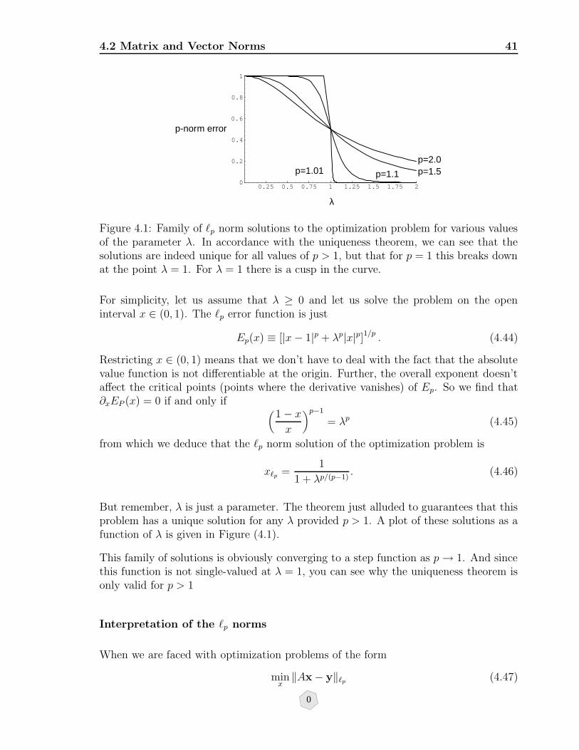
4.2 Matrix and Vector Norms 41
0.25 0.5 0.75 1 1.25 1.5 1.75 20
0.2
0.4
0.6
0.8
1
p=1.01 p=1.1 p=1.5 p=2.0
λ
p-norm error
Figure 4.1: Family of `p norm solutions to the optimization problem for various valuesof the parameter λ. In accordance with the uniqueness theorem, we can see that thesolutions are indeed unique for all values of p > 1, but that for p = 1 this breaks downat the point λ = 1. For λ = 1 there is a cusp in the curve.
For simplicity, let us assume that λ ≥ 0 and let us solve the problem on the openinterval x ∈ (0, 1). The `p error function is just
Ep(x) ≡ [|x− 1|p + λp|x|p]1/p . (4.44)
Restricting x ∈ (0, 1) means that we don’t have to deal with the fact that the absolutevalue function is not differentiable at the origin. Further, the overall exponent doesn’taffect the critical points (points where the derivative vanishes) of Ep. So we find that∂xEP (x) = 0 if and only if (
1− xx
)p−1
= λp (4.45)
from which we deduce that the `p norm solution of the optimization problem is
x`p =1
1 + λp/(p−1). (4.46)
But remember, λ is just a parameter. The theorem just alluded to guarantees that thisproblem has a unique solution for any λ provided p > 1. A plot of these solutions as afunction of λ is given in Figure (4.1).
This family of solutions is obviously converging to a step function as p→ 1. And sincethis function is not single-valued at λ = 1, you can see why the uniqueness theorem isonly valid for p > 1
Interpretation of the `p norms
When we are faced with optimization problems of the form
minx‖Ax− y‖`p (4.47)
0

42 A Little Linear Algebra
the question naturally arises: which p is best? There are two aspects of this question.The first is purely numerical. It turns out that some of the `p norms have more stablenumerical properties than others.
In particular, as we will see, p values near 1 are more stable than p values near 2.On the other hand, there is an important statistical aspect of this question. When weare doing inverse calculations, the vector y is associated with our data. If our datahave, say, a Gaussian distribution, then `2 is optimal in a certain sense to be describedshortly. On the other hand, if our data have the double-exponential distribution, then`1 is optimal. This optimality can be quantified in terms of the entropy or informationcontent of the distribution. For the Gaussian distribution we are used to thinking ofthis in terms of the variance or standard deviation. More generally, we can define the`p norm dispersion of a given probability density ρ(x) as
(σp)p ≡
∫ ∞
−∞|x− x0|pρ(x) dx (4.48)
where x0 is the center of the distribution. (The definition of the center need notconcern us here. The point is simply that the dispersion is a measure of how spreadout a probability distribution is.)
One can show (cf. [Tar87], Chapter 1) that for a fixed `p norm dispersion, the probabilitydensity with the minimum information content is given by the generalized gaussian
ρp(x) =p1−1/p
2σpΓ(1/p)exp
(−1
p
|x− x0|p(σp)p
)(4.49)
where Γ is the Gamma function [MF53]. These distributions are shown in Figure 4.2 forfour different values of p, 1, 2, 10, and ∞. The reason information content is so impor-tant is that being naturally conservative, we want to avoid jumping to any unduly riskyconclusions about our data. One way to quantify simplicity is in terms of informationcontent, or entropy: given two (or more) models which fit the data to the same degree,we may want to choose the one with the least information content in order to avoidover-interpreting the data. This is an important caveat for all of inverse theory.b Laterin the course we will come back to what it means to be “conservative” and see that thematter is more complicated than it might first appear.
4.3 Projecting Vectors Onto Other Vectors
Figure 4.3 illustrates the basic idea of projecting one vector onto another. We canalways represent one, say b, in terms of its components parallel and perpendicular tothe other. The length of the component of b along a is ‖b‖ cos θ which is also bTa/‖a‖
bThis is a caveat for all of life too. It is dignified with the title Occam’s razor after William ofOccam, an English philosopher of the early 14th century. What Occam actually wrote was: “Entianon sunt multiplicanda praeter necessitatem” (things should not be presumed to exist, or multiplied,beyond necessity).
0

4.3 Projecting Vectors Onto Other Vectors 43
p=10
p=2
p=infinity
p=1
Figure 4.2: Shape of the generalized Gaussian distribution for several values of p.
0

44 A Little Linear Algebra
b
a
a - b
b cos θθ
x
y
Figure 4.3: Let a and b be any two vectors. We can always represent one, say b, interms of its components parallel and perpendicular to the other. The length of thecomponent of b along a is ‖b‖ cos θ which is also bTa/‖a‖.
Now suppose we want to construct a vector in the direction of a but whose length isthe component of b along ‖b‖. We did this, in effect, when we computed the tangentialforce of gravity on a simple pendulum. What we need to do is multiply ‖b‖ cos θ by aunit vector in the a direction. Obviously a convenient unit vector in the a direction isa/‖a‖, which equals
a√aTa
.
So a vector in the a with length ‖b‖ cos θ is given by
‖b‖ cos θa =aTb
‖a‖a
‖a‖ (4.50)
=a
‖a‖aTb
‖a‖ =aaTb
aTa=
aaT
aTab (4.51)
As an exercise verify that in general a(aTb) = (aaT )b. This is not completely obvioussince in one expression there is an inner product in the parenthesis and in the otherthere is an outer product.
What we’ve managed to show is that the projection of the vector b into the directionof a can be achieved with the following matrix (operator)
aaT
aTa.
This is our first example of a projection operator.
0
4.4 Linear Dependence and Independence 45
4.4 Linear Dependence and Independence
Suppose we have n vectors
x1,x2, · · · ,xn (4.52)
of the same dimension. The question is, under what circumstances can the linearcombination of these vectors be zero:
α1x1 + α2x2 + · · ·αnxn = 0. (4.53)
If this is true with at least one of the coefficients αi nonzero, then we could isolatea particular vector on the right hand side, expressing it as a linear combination ofthe other vectors. In this case the original set of n vectors are said to be linearlydependent. On the other hand, if the only way for this sum of vectors to be zero isfor all the coefficients themselves to be zero, then we say that the vectors are linearlyindependent.
Now, this linear combination of vectors can also be written as a matrix-vector innerproduct. With a = (α1, α2, · · · , αn), and X = (x1,x2, · · · ,xn) we have the condition forlinear dependence being
Xa = 0 (4.54)
for some nonzero vector a, and the condition for linear independence being
Xa = 0⇒ a = 0. (4.55)
As a result, if we are faced with a linear system of equations to solve
Ax = b (4.56)
we can think in two different ways. On the one hand, we can investigate the equationin terms of the existence of a vector x satisfying the equation. On the other hand, wecan think in terms of the compatibility of the right hand side with the columns of thematrix.
Linear independence is also central to the notion of how big a vector space is–its di-mension. It’s intuitively clear that no two linearly independent vectors are adequateto represent an arbitrary vector in R3. For example, (1, 0, 0) and (0, 1, 0) are linearlyindependent, but there are no scalar coefficients that will let us write (1, 1, 1) as a linearcombination of the first two. Conversely, since any vector in R3 can be written as acombination of the three vectors (1, 0, 0), (0, 1, 0), and (0, 0, 1), it is impossible to havemore than three linearly independent vectors in R3.
The dimension of a space is the number of linearly independent vectors required torepresent an arbitrary element.
0

46 A Little Linear Algebra
4.5 The Four Fundamental Spaces
Suppose you have an n−dimensional space and n linearly independent vectors in thatspace. These vectors are said to be basis vectors since any element of the space canbe written as a linear combination of the basis vectors. For instance, two basis vectorsfor R2 are (1, 0) and (0, 1). Any element of R2 can be written as some constant times(1, 0) plus another constant times (0, 1). Any other pair of linearly independent vectorswould also work, such as (2, 0) and (1, 15).
OK, so take two basis vectors for R2 and consider all possible linear combinations ofthem. This the set of all vectors
α(1, 0) + β(0, 1),
where α and β are arbitrary scalars. This is called the span of the two vectors and inthis case it obviously consists of all of R2. The span of (1, 0) is just the x-axis in R2.
On the other hand, if we consider these two vectors as being in R3, so that we writethem as (1, 0, 0) and (0, 1, 0), then their span clearly doesn’t fill up all of R3. It does,however, fill up a subspace of R3, the x−y plane. The technical definition of a subspaceis that it is a subset closed under addition and scalar multiplication:
Definition 4 Subspaces: A subspace of a vector space is a nonempty subset S thatsatisfies
S1: The sum of any two elements from S is in S, and
S2: The scalar multiple of any element from S is in S.
If we take a general matrix A ∈ Rn×m, then the span of the columns must be asubspace of Rn. Whether this subspace amounts to the whole of Rn obviously dependson whether the columns are linearly independent or not. This subspace is called thecolumn space of the matrix and is usually denoted by R(A), for “range”. The dimensionof the column space is called the rank of the matrix.
Another fundamental subspace associated with any matrix A is associated with thesolutions of the homogeneous equation Ax = 0. Why is this a subspace? Take any twosuch solutions, say x and y and we have
A(x + y) = Ax + Ay = 0. (4.57)
Hence Similarly,A(αx) = αAx. (4.58)
This subspace is called the nullspace or kernel and is extremely important from thepoint of view of inverse theory. As we shall see, in an inverse calculation the right
0

4.5 The Four Fundamental Spaces 47
hand side of a matrix equations is usually associated with perturbations to the data.Vectors in the nullspace have no effect on the data and are therefore unresolved in anexperiment. Figuring out what features of a model are unresolved is a major goal ofinversion.
4.5.1 Spaces associated with a linear system Ax = y
The span of the columns is a subset of Rn and the span of the rows is a subset ofRm. In other words the rows of A have m components while the columns of A have ncomponents. Now the column space and the nullspace are generated by A. What aboutthe column space and the null space of AT ? These are, respectively, the row space andthe left nullspace of A. The nullspace and row space are subspaces of Rm, while thecolumn space and the left nullspace are subspaces of Rn.
Here is probably the most important result in linear algebra: For any matrix whatso-ever, the number of linearly independent rows equals the number of linearly independentcolumns. We summarize this by saying that row rank = column rank. For a genericn×m matrix, this is not an obvious result. If you haven’t encountered this before, itwould be a good idea to review a good linear algebra book, such as [Str88]. We cansummarize these spaces as follows:
Theorem 1 Fundamental Theorem of Linear Algebra Let A ∈ Rn×m. Then
1: Dimension of column space equals r, the rank.
2: Dimension of nullspace equals m− r.
3: Dimension of row space equals r.
4: Dimension of left nullspace equals n− r.
A Geometrical Picture
Any vector in the null space of a matrix, must be orthogonal to all the rows (since eachcomponent of the matrix dotted into the vector is zero). Therefore all the elements inthe null space are orthogonal to all the elements in the row space. In mathematical ter-minology, the null space and the row space are orthogonal complements of one another.Or, to say the same thing, they are orthogonal subspaces of Rm. Similarly, vectors inthe left null space of a matrix are orthogonal to all the columns of this matrix. Thismeans that the left null space of a matrix is the orthogonal complement of the columnspace; they are orthogonal subspaces of Rn. In other words, orthogonal complement ofa subspace S consists of all the vectors x such that (x, y) = 0 for y ∈ S.
0
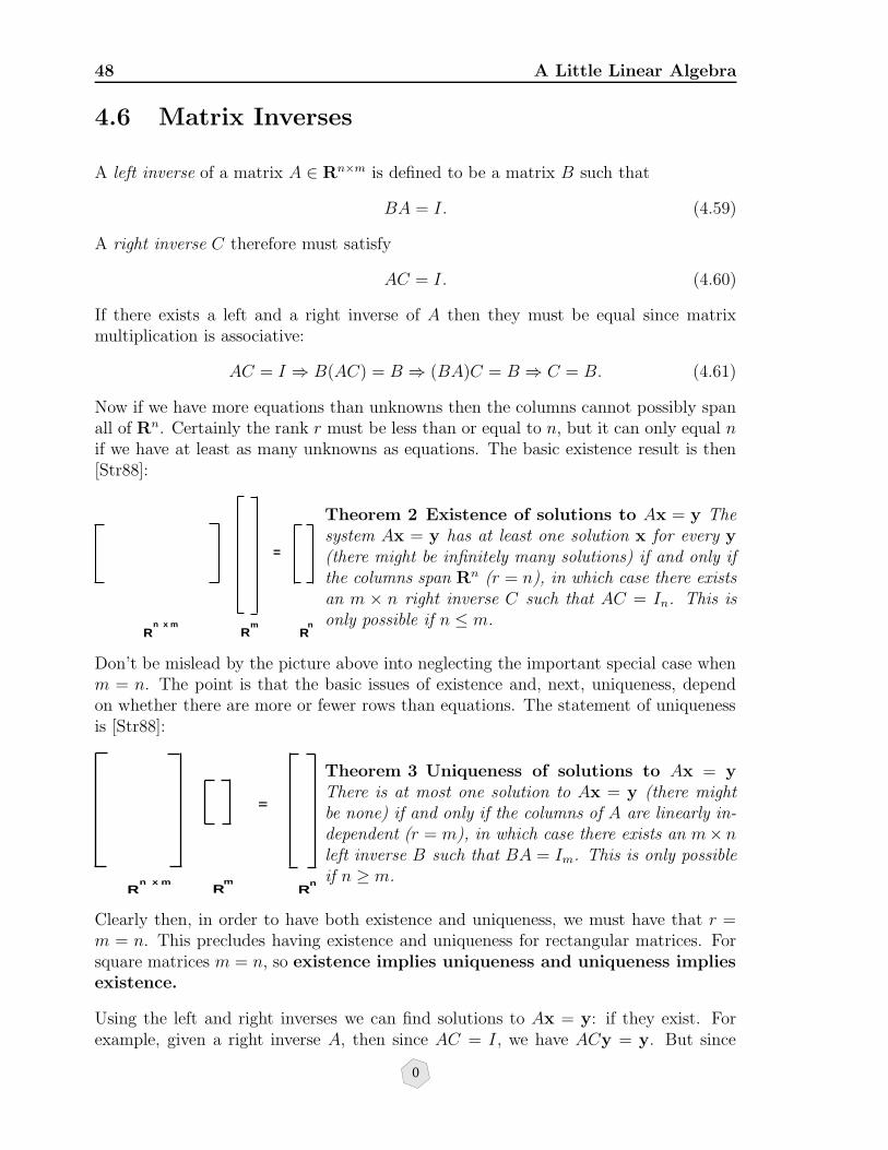
48 A Little Linear Algebra
4.6 Matrix Inverses
A left inverse of a matrix A ∈ Rn×m is defined to be a matrix B such that
BA = I. (4.59)
A right inverse C therefore must satisfy
AC = I. (4.60)
If there exists a left and a right inverse of A then they must be equal since matrixmultiplication is associative:
AC = I ⇒ B(AC) = B ⇒ (BA)C = B ⇒ C = B. (4.61)
Now if we have more equations than unknowns then the columns cannot possibly spanall of Rn. Certainly the rank r must be less than or equal to n, but it can only equal nif we have at least as many unknowns as equations. The basic existence result is then[Str88]:
R R R n x m n m
=
Theorem 2 Existence of solutions to Ax = y Thesystem Ax = y has at least one solution x for every y(there might be infinitely many solutions) if and only ifthe columns span Rn (r = n), in which case there existsan m × n right inverse C such that AC = In. This isonly possible if n ≤ m.
Don’t be mislead by the picture above into neglecting the important special case whenm = n. The point is that the basic issues of existence and, next, uniqueness, dependon whether there are more or fewer rows than equations. The statement of uniquenessis [Str88]:
R R R n x m n m
=
Theorem 3 Uniqueness of solutions to Ax = yThere is at most one solution to Ax = y (there mightbe none) if and only if the columns of A are linearly in-dependent (r = m), in which case there exists an m× nleft inverse B such that BA = Im. This is only possibleif n ≥ m.
Clearly then, in order to have both existence and uniqueness, we must have that r =m = n. This precludes having existence and uniqueness for rectangular matrices. Forsquare matrices m = n, so existence implies uniqueness and uniqueness impliesexistence.
Using the left and right inverses we can find solutions to Ax = y: if they exist. Forexample, given a right inverse A, then since AC = I, we have ACy = y. But since
0
4.7 Eigenvalues and Eigenvectors 49
Ax = y it follows that x = Cy. But C is not necessarily unique. On the other hand,if there exists a left inverse BA = I, then BAx = By, which implies that x = By.
Some examples. Consider first the case of more equations than unknowns n > m. Let
A =
−1 00 30 0
(4.62)
Since the columns are linearly independent and there are more rows than columns,there can be at most one solution. You can readily verify that any matrix of the form
[−1 0 γ0 1/3 ι
](4.63)
is a left inverse. The particular left inverse given by the formula (ATA)−1AT (cf. theexercise at the end of this chapter) is the one for which γ and ι are zero. But thereare infinitely many other left inverses. As for solutions of Ax = y, if we take the innerproduct of A with the vector (x1, x2)T we get
−x1
3x2
0
=
y1
y2
y3
(4.64)
So, clearly, we must have x1 = −y1 and x2 = 1/3y2. But, there will not be any solutionunless y3 = 0.
Next, let’s consider the case of more columns (unknowns) than rows (equations) n < m.Let
A =
[−1 0 00 3 0
](4.65)
Here you can readily verify that any matrix of the form−1 00 1/3γ ι
(4.66)
is a right inverse. The particular right inverse (shown in the exercise at the end of thischapter) AT (AAT )−1 corresponds to γ = ι = 0.
Now if we look at solutions of the linear system Ax = y with x ∈ R3 and y ∈ R2 wefind that x1 = −y1, x2 = 1/3y2, and that x3 is completely undetermined. So there isan infinite set of solutions corresponding to the different values of x3.
4.7 Eigenvalues and Eigenvectors
Usually when a matrix operates on a vector, it changes the direction of the vector. Butfor a special class of vectors, eigenvectors, the action of the matrix is to simply scale
0

50 A Little Linear Algebra
the vector:
Ax = λx. (4.67)
If this is true, then x is an eigenvector of the matrix A associated with the eigenvalueλ. Now, λx equals λIx so we can rearrange this equation and write
(A− λI)x = 0. (4.68)
Clearly in order that x be an eigenvector we must choose λ so that (A − λI) has anullspace and we must choose x so that it lies in that nullspace. That means we mustchoose λ so that Det(A − λI) = 0. This determinant is a polynomial in λ, called thecharacteristic polynomial. For example if
A =
[5 34 5
](4.69)
then the characteristic polynomial is
λ2 − 10λ+ 13 (4.70)
whose roots are
λ = 5 + 2√
3, and λ = 5− 2√
3. (4.71)
Now all we have to do is solve the two homogeneous systems:
[2√
3 3
4 2√
3
] [x1
x2
]= 0 (4.72)
and [−2√
3 3
4 −2√
3
] [x1
x2
]= 0 (4.73)
from which we arrive at the two eigenvectors
[ √3
2
1
],
[−√
32
1
](4.74)
But note well, that these eigenvectors are not unique. Because they solve a homogeneoussystem, we can multiply them by any scalar we like and not change the fact that theyare eigenvectors.
This exercise was straightforward. But imagine what would have happened if we hadneeded to compute the eigenvectors/eigenvalues of a 10× 10 matrix. Can you imaginehaving to compute the roots of a 10-th order polynomial? In fact, once you get pastorder 4, there is no algebraic formula for the roots of a polynomial. The eigenvalueproblem is much harder than solving Ax = y.
The following theorem gives us the essential computational tool for using eigenvectors.
0

4.7 Eigenvalues and Eigenvectors 51
Theorem 4 Matrix diagonalization Let A be an n× n matrix with n linearly inde-pendent eigenvectors. Let S be a matrix whose columns are these eigenvectors. ThenS−1AS is a diagonal matrix Λ whose elements are the eigenvalues of A.
The proof is easy. The elements in the first column of the product matrix AS areprecisely the elements of the vector which is the inner product of A with the firstcolumn of S. The first column of S, say s1, is, by definition, an eigenvector of A.Therefore the first column of AS is λ1s1. Since this is true for all the columns, itfollows that AS is a matrix whose columns are λisi. But now we’re in business since
[λ1s1 λ2s2 · · ·λnsn] = [s1 s2 · · · sn] diag(λ1, λ2, · · · , λn) ≡ SΛ. (4.75)
Therefore AS = SΛ which means that S−1AS = Λ. S must be invertible since we’veassumed that all it’s columns are linearly independent.
Some points to keep in mind:
• Any matrix in Rn×n with n distinct eigenvalues can be diagonalized.
• Because the eigenvectors themselves are not unique, the diagonalizing matrix Sis not unique.
• Not all square matrices possess n linearly independent eigenvectors.
• A matrix can be invertible without being diagonalizable.
We can summarize these ideas with a theorem whose proof can be found in linearalgebra books.
Theorem 5 Linear independence of eigenvectors If n eigenvectors of an n × nmatrix correspond to n different eigenvalues, then the eigenvectors are linearly indepen-dent.
An important class of matrices for inverse theory are the real symmetric matrices. Thereason is that since we have to deal with rectangular matrices, we often end up treatingthe matrices ATA and AAT instead. And these two matrices are manifestly symmetric.In the case of real symmetric matrices, the eigenvector/eigenvalue decomposition isespecially nice, since in this case the diagonalizing matrix S can be chosen to be anorthogonal matrix Q.
Theorem 6 Orthogonal decomposition of a real symmetric matrix A real sym-metric matrix A can be factored into
A = QΛQT (4.76)
with orthonormal eigenvectors in Q and real eigenvalues in Λ.
0
52 A Little Linear Algebra
4.8 Orthogonal decomposition of rectangular ma-
trices
For dimensional reasons there is clearly no hope of the kind of eigenvector decompositiondiscussed above being applied to rectangular matrices. However, there is an amazinglyuseful generalization that pertains if we allow a different orthogonal matrix on each sideof A. It is called the Singular Value Decomposition (SVD) and works for any matrixwhatsoever. Essentially the singular value decomposition generates orthogonal basesof Rm and Rn simultaneously.
Theorem 7 Singular value decomposition Any matrix A ∈ Rn×m can be factoredas
A = UΛV T (4.77)
where the columns of U ∈ Rn×n are eigenvectors of AAT and the columns of V ∈ Rm×m
are the eigenvectors of ATA. Λ ∈ Rn×m is a rectangular matrix with the singular valueson its main diagonal and zero elsewhere. The singular values are the square roots of theeigenvalues of ATA, which are the same as the nonzero eigenvalues of AAT . Further,there are exactly r nonzero singular values, where r is the rank of A.
The columns of U and V span the four fundamental subspaces. The column space of Ais spanned by the first r columns of U . The row space is spanned by the first r columnsof V . The left nullspace of A is spanned by the last n − r columns of U . And thenullspace of A is spanned by the last m− r columns of V .
A direct approach to the SVD, due to the physicist Lanczos[Lan61], is to make asymmetric matrix out of the rectangular matrix A as follows: Let
S =
[0 AAT 0
]. (4.78)
Since A is in Rn×m, S must be in R(n+m)×(n+m).
m by n or n by m? For the rest of this book we will interpret the matrix Aas mapping from the space of model parameters into the space of data–the forwardproblem. So there are m parameters and n data. But, obviously this is unnecessaryfor the interpretation of the results. Model space is simply Rm and data space is Rn.
And since S is symmetric it has orthogonal eigenvectors wi with real eigenvalues λi
Swi = λiwi. (4.79)
If we split up the eigenvector wi, which is in Rn+m, into an n-dimensional data partand an m-dimensional model part
wi =
[uivi
](4.80)
0
4.8 Orthogonal decomposition of rectangular matrices 53
then the eigenvalue problem for S reduces to two coupled eigenvalue problems, one forA and one for AT
ATui = λivi (4.81)
Avi = λiui. (4.82)
We can multiply the first of these equations by A and the second by AT to get
ATAvi = λi2vi (4.83)
AATui = λi2ui. (4.84)
So we see, once again, that the model eigenvectors ui are eigenvectors of AAT and thedata eigenvectors vi are eigenvectors of ATA. Also note that if we change sign of theeigenvalue we see that (−ui,vi) is an eigenvector too. So if there are r pairs of nonzeroeigenvalues ±λi then there are r eigenvectors of the form (ui,vi) for the positive λi andr of the form (−ui,vi) for the negative λi.
Keep in mind that the matrices U and V whose columns are the date and modeleigenvectors are square (respectively n× n and m×m) and orthogonal. Therefore wehave UTU = UUT = In and V TV = V V T = Im. But it is important to distinguishbetween the eigenvectors associated with zero and nonzero eigenvalues. Let Ur andVr be the matrices whose columns are the r model and data eigenvectors associatedwith the r nonzero eigenvalues and U0 and V0 be the matrices whose columns arethe eigenvectors associated with the zero eigenvalues, and let Λr be the r × r square,diagonal matrix containing the r nonzero eigenvalues. Then we have by 4.81 and 4.82the following eigenvalue problem
AVr = UrΛr (4.85)
ATUr = VrΛr (4.86)
AV0 = 0 (4.87)
ATU0 = 0. (4.88)
Since the full matrices U and V satisfy UTU = UUT = In and V TV = V V T = Im itcan be readily seen that AV = UΛ implies A = UΛV T and therefore
A = [Ur, U0]
[Λr 00 0
] [V Tr
V T0
]= UrΛrV
Tr , (4.89)
This is the singular value decomposition. Notice that 0 represent rectangular matricesof zeros. Since Λr is r × r and Λ is n × m then the lower left block of zeros must ben− r× r, the upper right must be r×m− r and the lower right must be n− r×m− r.
It is important to keep the subscript r in mind since the fact that A can be recon-structed from the eigenvectors associated with the nonzero eigenvalues means that the
0
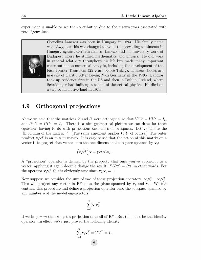
54 A Little Linear Algebra
experiment is unable to see the contribution due to the eigenvectors associated withzero eigenvalues.
Cornelius Lanczos was born in Hungary in 1893. His family namewas Lowy, but this was changed to avoid the prevailing sentiments inHungary against German names. Lanczos did his university work atBudapest where he studied mathematics and physics. He did workin general relativity throughout his life but made many importantcontributions to numerical analysis, including the development of theFast Fourier Transform (25 years before Tukey). Lanczos’ books aremarvels of clarity. After fleeing Nazi Germany in the 1930s, Lanczostook up residence first in the US and then in Dublin, Ireland, whereSchrodinger had built up a school of theoretical physics. He died ona trip to his native land in 1974.
4.9 Orthogonal projections
Above we said that the matrices V and U were orthogonal so that V TV = V V T = Imand UTU = UUT = In. There is a nice geometrical picture we can draw for theseequations having to do with projections onto lines or subspaces. Let vi denote theith column of the matrix V . (The same argument applies to U of course.) The outerproduct viv
Ti is an m×m matrix. It is easy to see that the action of this matrix on a
vector is to project that vector onto the one-dimensional subspace spanned by vi:
(viv
Ti
)x = (vTi x)vi.
A “projection” operator is defined by the property that once you’ve applied it to avector, applying it again doesn’t change the result: P (Px) = Px, in other words. Forthe operator viv
Ti this is obviously true since vTi vi = 1.
Now suppose we consider the sum of two of these projection operators: vivTi + vjv
Tj .
This will project any vector in Rm onto the plane spanned by vi and vj. We cancontinue this procedure and define a projection operator onto the subspace spanned byany number p of the model eigenvectors:
p∑
i=1
vivTi .
If we let p = m then we get a projection onto all of Rm. But this must be the identityoperator. In effect we’ve just proved the following identity:
m∑
i=1
vivTi = V V T = I.
0
4.10 A few examples 55
On the other hand, if we only include the terms in the sum associated with the r nonzerosingular values, then we get a projection operator onto the non-null space (which is therow space). So
r∑
i=1
vivTi = VrV
Tr
is a projection operator onto the row space. By the same reasoning
m∑
i=r+1
vivTi = V0V
T0
is a projection operator onto the null space. Putting this all together we can say that
VrVTr + V0V
T0 = I.
This says that any vector in Rm can be written in terms of its component in the nullspace and its component in the row space of A. Let x ∈ Rm, then
x = Ix =(VrV
Tr + V0V
T0
)x = (x)row + (x)null. (4.90)
4.10 A few examples
This example shows that often matrices with repeated eigenvalues cannot be diagonal-ized. But symmetric matrices can always be diagonalized.
A =
[3 10 3
](4.91)
The eigenvalues of this matrix are obviously 3 and 3. This matrix has a one-dimensionalfamily of eigenvectors; any vector of the form (x, 0)T will do. So it cannot be diagonal-ized, it doesn’t have enough eigenvectors.
Now consider
A =
[3 00 3
](4.92)
The eigenvalues of this matrix are still 3 and 3. But it will be diagonalized by anyinvertible matrix! So, of course, to make our lives simple we will choose an orthogonalmatrix. How about
[0 11 0
]? (4.93)
0

56 A Little Linear Algebra
That will do. But so will1√2
[−1 11 1
]. (4.94)
So, as you can see, repeated eigenvalues give us choice. And for symmetric matrices wenearly always choose to diagonalize with orthogonal matrices.
Exercises
1. Give specific (nonzero) examples of 2 by 2 matrices satisfying the following prop-erties:
A2 = 0, A2 = −I2, and AB = −BA (4.95)
2. Let A be an upper triangular matrix. Suppose that all the diagonal elementsare nonzero. Show that the columns must be linearly independent and that thenull-space contains only the zero vector.
3. Figure out the column space and null space of the following two matrices:[
1 −10 0
]and
[0 0 00 0 0
](4.96)
4. Which of the following two are subspaces of Rn: the plane of all vectors whosefirst component is zero; the plane of all vectors whose first component is 1.
5. Let
x =
[9−12
]. (4.97)
Compute ‖x‖1, ‖x‖2, and ‖x‖∞.
6. Define the unit `p-ball in the plane R2 as the set of points satisfying
‖x‖`p ≤ 1. (4.98)
Draw a picture of this ball for p = 1, 2, 3 and ∞.
7. Show that B = (ATA)−1AT is a left inverse and C = AT (AAT )−1 is a right inverseof a matrix A, provided that AAT and ATA are invertible. It turns out that ATAis invertible if the rank of A is equal to n, the number of columns; and AAT isinvertible if the rank is equal to m, the number of rows.
8. Consider the matrix [a bc d
](4.99)
The trace of this matrix is a + d and the determinant is ad− cb. Show by directcalculation that the product of the eigenvalues is equal to the determinant andthe sum of the eigenvalues is equal to the trace.
0
BIBLIOGRAPHY 57
9. As we have seen, an orthogonal matrix corresponds to a rotation. Consider theeigenvalue problem for a simple orthogonal matrix such as
Q =
[0 −11 0
](4.100)
How can a rotation map a vector into a multiple of itself?
10. Show that the eigenvalues of Aj are the j-th powers of the eigenvalues of A.
11. Using the SVD show thatAAT = UΛΛTU (4.101)
andATA = V ΛTΛV. (4.102)
The diagonal matrices ΛΛT ∈ Rm×m and ΛTΛ ∈ Rn×n have different dimensions,but they have the same r nonzero elements: σ1, σ2, · · · , σr.
12. Compute the SVD of the matrix
A =
1 1 00 0 10 0 −1
(4.103)
directly by computing the eigenvectors of ATA and AAT . Show that the pseu-doinverse solution to the linear system Ax = y where y = (1, 2, 1)T is given byaveraging the equations.
13. Prove that (Ax,y) = (x, ATy).
14. Prove that if Q is an orthogonal matrix, that Qx is a rotation of x.
15. What happens to the `p norm if p < 1? For example, is
(n∑
i=1
|xi|1/2)2
(4.104)
a norm?
Bibliography
[GvL83] G. Golub and C. van Loan. Matrix Computations. Johns Hopkins, Baltimore,1983.
[Lan61] C. Lanczos. Linear Differential Operators. D. van Nostrand, 1961.
[MF53] P.M. Morse and H. Feshbach. Methods of Theoretical Physics. McGraw Hill,1953.
0

58 BIBLIOGRAPHY
[SG88] J.A. Scales and A. Gersztenkorn. Robust methods in inverse theory. InverseProblems, 4:1071–1091, 1988.
[Str88] G. Strang. Linear Algebra and its Application. Saunders College Publishing,Fort Worth, 1988.
[Tar87] A. Tarantola. Inverse Problem Theory. Elsevier, New York, 1987.
0

Chapter 5
SVD and Resolution in LeastSquares
In section 4.8 we introduced the singular value decomposition (SVD). The SVD is anatural generalization of the eigenvector decomposition to arbitrary (even rectangular)matrices. It plays a fundamental role in linear inverse problems.
5.0.1 A Worked Example
Let’s begin by doing a worked example. Suppose that
A =
[1 1 00 0 1
]
and hence that
AT =
1 01 00 1
, ATA =
1 1 01 1 00 0 1
, AAT =
[2 00 1
]
The eigenvalue problem for AAT is easy; since it is diagonal, its diagonal entries arethe eigenvalues. To find the eigenvalues of ATA we need to find the roots of thecharacteristic polynomial
Det
∣∣∣∣∣∣∣
1− λ 1 01 1− λ 00 0 1− λ
∣∣∣∣∣∣∣= (1− λ)
[(1− λ)2 − 1
]= 0
which are 2, 1 and 0.
Now we can compute the data eigenvectors ui by solving the eigenvalue problem
1
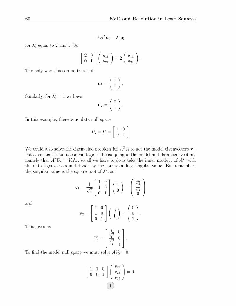
60 SVD and Resolution in Least Squares
AATui = λ2iui
for λ2i equal to 2 and 1. So
[2 00 1
](u11
u21
)= 2
(u11
u21
).
The only way this can be true is if
u1 =
(10
).
Similarly, for λ2i = 1 we have
u2 =
(01
).
In this example, there is no data null space:
Ur = U =
[1 00 1
]
We could also solve the eigenvalue problem for ATA to get the model eigenvectors vi,but a shortcut is to take advantage of the coupling of the model and data eigenvectors,namely that ATUr = VrΛr, so all we have to do is take the inner product of AT withthe data eigenvectors and divide by the corresponding singular value. But remember,the singular value is the square root of λ2, so
v1 =1√2
1 01 00 1
(
10
)=
1√2
1√2
0
and
v2 =
1 01 00 1
(
01
)=
001
.
This gives us
Vr =
1√2
01√2
0
0 1
.
To find the model null space we must solve AV0 = 0:
[1 1 00 0 1
]v13
v23
v33
= 0.
1

61
This means that v13 + v23 = 0 and v33 = 0, so the normalized model null space singularvector is
V0 =
− 1√2
1√2
0
.
We can verify the SVD directlyA = UrΛrV
Tr
=
[1 00 1
] [ √2 0
0 1
]
1√2
01√2
0
0 1
T
=
[1 1 00 0 1
]
Remember, the only way that there can be no null space at all (no U0 or V0) is ifn = m = r.
5.0.2 The Generalized Inverse
Recall the SVD of A is A = UΛV T . U is n× n, V is m ×m and Λ is n×m. If thereare no zero singular values the following matrix provides a one-sided inverse of A:
A† = V Λ−1UT
where Λ−1 refers to the m × n matrix with 1/λi on its main diagonal. The matrix A†
is called the generalized inverse of A, or the pseudo-inverse. Be careful to keep thedimensions straight; in the SVD
A = UΛV T
we know that V must be m×m (its columns span model space) and U must be n× n(its columns span data space). Therefore Λ must be n×m. Similarly if we write
V Λ−1UT
it is clear that Λ−1 must refer to an m× n matrix. a
Whether A† will be a left inverse or a right inverse depends on whether there are moreequations than unknowns (n ≥ m) or fewer (m ≥ n). There is a two-sided (ordinary)inverse if and only if m = n = r, where r is the rank. To see how this goes consider aconcrete case, m = 3 and n = r = 2 So
Λ =
[λ1 0 00 λ2 0
]n×m
aFor this reason perhaps it is an abuse of notation to write Λ−1. Perhaps we should write Λ† instead.The main danger of the current notation is that one is tempted to assume that Λ−1Λ = ΛΛ−1 = I ,which, as we have seen is not true in general.
1

62 SVD and Resolution in Least Squares
and hence
Λ−1 =
1/λ1 00 1/λ2
0 0
. m× n
Since A† is V Λ−1UT then
A†A = V Λ−1UTUΛV T = V Λ−1ΛV T .
Unfortunately we cannot simply replace Λ−1Λ by the identity:
1/λ1 00 1/λ2
0 0
[λ1 0 00 λ2 0
]=
1 0 00 1 00 0 0
.
ThereforeV Λ−1ΛV T 6= I.
On the other hand if we multiply A on the right by A† we get
AA† = UΛΛ−1UT .
And
ΛΛ−1 =
[λ1 0 00 λ2 0
]
1/λ1 00 1/λ2
0 0
=
[1 00 1
].
So in this case we can see that A† is a right inverse but not a left inverse. You canverify for yourself that if there were more unknowns than data (n ≥ m), A† would bea left inverse of A.
If there are zero singular values, then the only thing different we must do is project outthose components. The SVD then becomes:
A = UrΛrVTr .
The generalized inverse is then defined to be
A† ≡ VrΛ−1r UT
r .
Note that in this case Λr is an r × r matrix so
A†A = VrVTr
andAA† = UrU
Tr .
The first of these is an identity matrix only if r = m and the second only if r = n. Youwill show in an exercise however that in any case
A†AA† = A†
AA†A = A
Let us explore the significance of the generalized inverse bit by bit. This discussion ispatterned on that in Chapter 12 of [AR80].
1

63
No Null Space
First consider the case in which there is no data or model null space. This can onlyhappen when r = m = n, in which case the generalized inverse is the ordinary inverse.
A Data Null Space
Next consider the case in which there is a data null space U0 but no model null space(n > m). Since ATU0 = 0, it follows that UT
0 A = 0. And hence, the forward operatorA always maps models into vectors that have no component in U0. That means that ifthere is a data null space, and if the data have a component in this null space,then it will be impossible to fit them exactly.
That being the case, it would seem reasonable to try to minimize the misfit betweenobserved and predicted data, say,
min ‖Am− d‖2, (5.1)
where m is an element of the model space. I.e., least-squares. A least-squares minimiz-ing model must be associated with a critical point of this mis-fit function. Differenti-ating Equation 5.1 with respect to m and setting the result equal to zero results in thenormal equations:
ATAm = ATd. (5.2)
There are many ways to derive the normal equations. In the next section we will derivethem without using any calculus. But it is not too hard to do the differentiation inEquation 5.1. First, write the norm-squared as an inner product:
‖Am− d‖2 = (Am− d, Am− d).
Expand this. You’ll get a sum of 4 inner products, such as (Am, Am). You candifferentiate these with respect to each of the components of m if you like, but youcan do this in vector notation with a little practice. For instance, the derivative of(m,m) with respect to m is 2m. The derivative of (m, a) (which equals (a,m))with respect to m is a. Further, since (Am, Am) = (ATAm,m) = (m, ATAm), thederivative of (Am, Am) with respect to m is 2ATAm. You can move A back and forthacross the inner product just by taking the transpose.
Now, by Equation 4.89
ATA = (UrΛrVTr )TUrΛrV
Tr = VrΛ
Tr U
Tr UrΛrV
Tr .
At this point we have to be a bit careful. We can be sure that UUT = UTU = In, ann-dimensional identity. And that V V T = V TV = Im. But this is not true of Vr if there
1
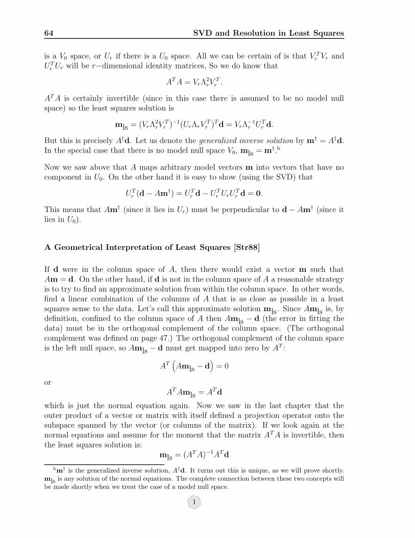
64 SVD and Resolution in Least Squares
is a V0 space, or Ur if there is a U0 space. All we can be certain of is that V Tr Vr and
UTr Ur will be r−dimensional identity matrices, So we do know that
ATA = VrΛ2rV
Tr .
ATA is certainly invertible (since in this case there is assumed to be no model nullspace) so the least squares solution is
mls = (VrΛ2rV
Tr )−1(UrΛrV
Tr )Td = VrΛ
−1r UT
r d.
But this is precisely A†d. Let us denote the generalized inverse solution by m† = A†d.In the special case that there is no model null space V0, mls = m†.b
Now we saw above that A maps arbitrary model vectors m into vectors that have nocomponent in U0. On the other hand it is easy to show (using the SVD) that
UTr (d− Am†) = UT
r d− UTr UrU
Tr d = 0.
This means that Am† (since it lies in Ur) must be perpendicular to d− Am† (since itlies in U0).
A Geometrical Interpretation of Least Squares [Str88]
If d were in the column space of A, then there would exist a vector m such thatAm = d. On the other hand, if d is not in the column space of A a reasonable strategyis to try to find an approximate solution from within the column space. In other words,find a linear combination of the columns of A that is as close as possible in a leastsquares sense to the data. Let’s call this approximate solution mls. Since Amls is, bydefinition, confined to the column space of A then Amls − d (the error in fitting thedata) must be in the orthogonal complement of the column space. (The orthogonalcomplement was defined on page 47.) The orthogonal complement of the column spaceis the left null space, so Amls − d must get mapped into zero by AT :
AT(Amls − d
)= 0
orATAmls = ATd
which is just the normal equation again. Now we saw in the last chapter that theouter product of a vector or matrix with itself defined a projection operator onto thesubspace spanned by the vector (or columns of the matrix). If we look again at thenormal equations and assume for the moment that the matrix ATA is invertible, thenthe least squares solution is:
mls = (ATA)−1ATd
bm† is the generalized inverse solution, A†d. It turns out this is unique, as we will prove shortly.mls is any solution of the normal equations. The complete connection between these two concepts willbe made shortly when we treat the case of a model null space.
1

65
Now A applied to the least squares solution is the approximation to the data fromwithin the column space. So Amls is precisely the projection of the data d onto thecolumn space:
Amls = A(ATA)−1ATd.
Before when we did orthogonal projections, the projecting vectors/matrices were or-thogonal, so the ATA term would have been the identity, but the outer product structurein Amls is evident.
The generalized inverse projects the data onto the column space of A.
A few observations:
• When A is invertible (square, full rank) A(ATA)−1AT = AA−1(AT )−1AT = I, soevery vector projects onto itself.
• ATA has the same null space as A. Proof: clearly if Am = 0, then ATAm = 0.Going the other way, suppose ATAm = 0. Then mTATAm = 0. But this canalso be written as (Am, Am) = ‖Am‖2 = 0. By the properties of the norm,‖Am‖2 = 0⇒ Am = 0.
• As a corollary of this, if A has linearly independent columns (i.e., the rank r = m)then ATA is invertible.
A Model Null Space
Now let us consider the existence of a model null space V0 (but no data null space U0),so m > n ≥ r. Once again, using the SVD, we can show that (since m† = A†d)
Am† = AA†d = UrΛrVTr VrΛ
−1r UT
r d = d
since V Tr Vr = Ir and UrU
Tr = Ir = In. But since m† is expressible in terms of the Vr
vectors (and not the V0 vectors), it is clear that the generalized inverse solution is amodel that satisfies Am† = d but is entirely confined to Vr.
A consequence of this is that an arbitrary least squares solution (i.e., any solution ofthe normal equations) can be represented as the sum of the generalized solution withsome component in the model null space:
mls = m† +M∑
i=r+1
αivi (5.3)
1
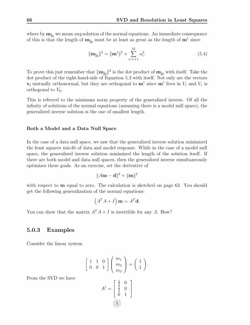
66 SVD and Resolution in Least Squares
where by mls we mean any solution of the normal equations. An immediate consequenceof this is that the length of mls must be at least as great as the length of m† since
‖mls‖2 = ‖m†‖2 +M∑
i=r+1
α2i . (5.4)
To prove this just remember that ‖mls‖2 is the dot product of mls with itself. Take thedot product of the right-hand-side of Equation 5.3 with itself. Not only are the vectorsvi mutually orthonormal, but they are orthogonal to m† since m† lives in Vr and Vr isorthogonal to V0.
This is referred to the minimum norm property of the generalized inverse. Of all theinfinity of solutions of the normal equations (assuming there is a model null space), thegeneralized inverse solution is the one of smallest length.
Both a Model and a Data Null Space
In the case of a data null space, we saw that the generalized inverse solution minimizedthe least squares mis-fit of data and model response. While in the case of a model nullspace, the generalized inverse solution minimized the length of the solution itself. Ifthere are both model and data null spaces, then the generalized inverse simultaneouslyoptimizes these goals. As an exercise, set the derivative of
‖Am− d‖2 + ‖m‖2
with respect to m equal to zero. The calculation is sketched on page 63. You shouldget the following generalization of the normal equations:
(ATA+ I
)m = ATd.
You can show that the matrix ATA+ I is invertible for any A. How?
5.0.3 Examples
Consider the linear system
[1 1 00 0 1
]m1
m2
m3
=
(11
).
From the SVD we have
A† =
12
012
00 1
.
1

67
It is obvious that m3 = 1 and that there are not enough equations to specify m1 or m2.All we can say at this point is that m1 + m2 = 1. Some possible solutions then are:m1 = 0, m2 = 1, m1 = 1, m2 = 0, m1 = .5, m2 = .5, and so on. All of these choicesexplain the “data”.
The generalized inverse solution is A†d = (1/2, 1/2, 1)T . Here we see the key feature ofleast squares (or generalized inverses): when faced with uncertainty least squares splitsthe difference.
5.0.4 Resolution
Resolution is all about how precisely one can infer model parameters from data. Theissue is complicated by all of the uncertainties that exist in any inverse problem: un-certainties in the forward modeling, the discretization of the model itself (i.e., replacingcontinuous functions by finite-dimensional vectors), noise in the data, and uncertain-ties in the constraints or a priori information we have. This is why we need a fairlyelaborate statistical machinery to tackle such problems. However, there are situationsin which resolution becomes relatively straightforward–whether these situations pertainin practice is another matter.
One of these occurs when the problem is linear and the only uncertainties arise fromrandom noise in the data. In this case the true Earth model is linearly related to theobserved data by d = Am+e where e is an n-dimensional vector of random errors. Themeaning of this equation is as follows: if there were no random noise in the problem,e would be zero and the true Earth model would predict the data exactly (d = Am).We could then estimate the true model by applying the pseudo-inverse of A to themeasurements. On the other hand, if e is nonzero, d = Am + e, we still get thegeneralized inverse solution by applying the pseudo-inverse to the data: m† = A†d. Itfollows that
m† = A† (Am + e) . (5.5)
Later on we will discuss the error term explicitly. For now we can finesse the issue byassuming that the errors have zero mean, in which case if we simply take the averageof Equation 5.5 the error term goes away.c For now let’s simply assume that the errorsare zero
m† = A†Am. (5.6)
This result can be interpreted as saying that the matrix A†A acts as a kind of filterrelating the true Earth model to the computed Earth model. Thus, if A†A were equal
cAfter we discuss probability in more detail we would take expectations as follows:
E[m†] = E[A† (Am + e)] = A†Am +A†E[e] = A†Am
since if the data have zero mean, E[e] = 0.
1

68 SVD and Resolution in Least Squares
to the identity matrix, we would have perfect resolution. Using the SVD we have
m† = VrΛ−1r UT
r UrΛrVTr m = VrV
Tr m.
We can use UTr Ur = I whether there is a data null space or not. So in any case the
matrix VrVTr is the “filter” relating the computed Earth parameters to the true ones.
In the example above, with
A =
[1 1 00 0 1
]
the resolution matrix VrVTr is equal to
1√2
1√2
01√2
1√2
0
0 0 1
.
This says that the model parameter m3 is perfectly well resolved, but that we can onlyresolve the average of the first two parameters m1 and m2. The more nonzero terms thatappear in the rows of the resolution matrix, the more broadly averaged our inferencesof the model parameters.
Data resolution is connected to the fact that the observed data may be different thanthe data predicted by the generalized inverse. The latter is just Am†. But this is AA†d.So if we call this d†, then we have a relation very similar to that given by the resolutionmatrix:
d† = AA†d = UrΛrVTr VrΛ
−1r UT
r d = UrUTr d
so we can think of the matrix UrUTr as telling us about how well the data are predicted
by the computed model. In our example above, there is no data null space, so the dataare predicted perfectly. But if there is a data null space then the row vectors of UrU
Tr
will represent averages of the data.Exercises
1. Verify the following two “Penrose conditions”:
A†AA† = A†
AA†A = A
2. Show that minimizing‖Am− d‖2 + λ‖m‖2
with respect to m leads to the following generalized “normal equations”(ATA+ λI
)m = ATd.
3. Show that ATA + λI is always an invertible matrix.
1

BIBLIOGRAPHY 69
Bibliography
[AR80] K. Aki and P. Richards. Quantitave Seismology: Theory and Practice. Freeman,1980.
[Str88] G. Strang. Linear Algebra and its Application. Saunders College Publishing,Fort Worth, 1988.
1

70 BIBLIOGRAPHY
1

Chapter 6
A Summary of Probability andStatistics
Collected here are a few basic definitions and ideas. Fore more details consult a textbookon probability or mathematical statistics, for instance [Sin91], [Par60], and [Bru65].We begin with a discussion of discrete probabilites, which involves counting sets. Thenwe introduce the notion of a numerical valued random variable and random physicalphenomena. The main goal of this chapter is to develope the tools we need to charac-terize the uncertainties in both geophysical data sets and in the description of Earthmodels—at least when we have our Bayesian hats on. So the chapter culminates with adiscussion of various descriptive statistics numerical data (means, variances, etc). Mostof the problems that we face in geophysics involves spatially or temporally varyingrandom phenomena, also known as stochastic processes; e.g., velocity as a function ofspace. For everything we will do in this course, however, it suffices to consider only finitedimensional vector-valued random variables, such as we would measure by sampling arandom function at discrete times or spatial locations.
6.1 Sets
Probability is fundamentally about measuring sets. The sets can be finite, as in thepossible outcomes of a toss of a coin, or infinite, as in the possible values of a measuredP-wave impedance. The space of all possible outcomes of a given experiment is calledthe sample space. We will usually denote the sample space by Ω. If the problem issimple enough that we can enumerate all possible outcomes, then assigning probabilitiesis easy.
0

72 A Summary of Probability and Statistics
!#"#$#%#&#'!#"#$#%#&#'!#"#$#%#&#'!#"#$#%#&#'!#"#$#%#&#'
Ω
A
B
C
(*)*+*,*-*.*/*0(*)*+*,*-*.*/*0(*)*+*,*-*.*/*0(*)*+*,*-*.*/*0(*)*+*,*-*.*/*0(*)*+*,*-*.*/*0
A U (B - C) C - B B C - (A U B U C)
U
Ω
Figure 6.1: Examples of the intersection, union, and complement of sets.
Example 1
Toss a fair die twice. By “fair” we mean that each of the 6 possible outcomes is equallylikely. The sample space for this experiment consists of 1, 2, 3, 4, 5, 6. There are sixpossible equally likely outcomes of tossing the die. There is only one way to get anygiven number 1 − 6, therefore if A is the event that we toss a 4, then the probabilityassociated with A, which we will call P (A) is
P (A) =N(A)
N(Ω)=
1
6(6.1)
where we use N(A) to denote the number of possible ways of achieving event A andN(Ω) is the size of the sample space.
6.1.1 More on Sets
The union of two sets A and B consists of all those elements which are either in A orB; this is denoted by A∪B or A+B The intersection of two sets A and B consists ofall those elements which are in both A and B; this is denoted by A ∩B or simply AB.The complement of a set A relative to another set B consists of those elements whichare in A but not in B; this is denoted by A− B. Often, the set B is this relationshipis the entire sample space, in which case we speak simply of the complement of A anddenote this by Ac. These ideas are illustrated in Figure 6.1
0

6.1 Sets 73
The set with no elements in it is called the empty set and is denoted ∅. Its probabilityis always 0
P (∅) = 0. (6.2)
Since, by definition, the sample space contains all possible outcomes, its probabilitymust always be 1
P (Ω) = 1. (6.3)
The other thing we need to be able to do is combine probabilities:a
P (A ∪ B) = P (A) + P (B)− P (AB). (6.4)
P (AB) is the probability of the event A intersect B, which means the event A and B.In particular, if the two events are exclusive, i.e., if AB = 0 then
P (A ∪ B) = P (A) + P (B). (6.5)
This result extends to an arbitrary number of exclusive events Ai
P (A1 ∪ A2 ∪ · · · ∪ An) =n∑
i=1
P (Ai). (6.6)
This property is called additivity. Events A and B are said to be independent ifP (AB) = P (A)P (B).
Example 2
Toss the fair die twice. The sample space for this experiment consists of
1, 1, 1, 2, . . .6, 5, 6, 6. (6.7)
Let A be the event that the first number is a 1. Let B be the event that the secondnumber is a 2. The the probability of both A and B occurring is the probability of theintersection of these two sets. So
P (AB) =N(AB)
N(Ω)=
1
36(6.8)
Example 3
A certain roulette wheel has 4 numbers on it: 1, 2, 3, and 4. The even numbers arewhite and the odd numbers are black. The sample space associated with spinning thewheel twice is
1, 1, 1, 2, 1, 3, 1, 4aThat P (A ∪B) = P (A) + P (B) for exclusive events is a fundamental axiom of probability.
0

74 A Summary of Probability and Statistics
2, 1, 2, 2, 2, 3, 2, 43, 1, 3, 2, 3, 3, 3, 44, 1, 4, 2, 4, 3, 4, 4
Now, in terms of black and white, the different outcomes are
black, black, black,white, black, black, black,white
white, black, white,white, white, black, white,whiteblack, black, black,white, black, black, black,whitewhite, black, white,white, white, black, white,white
Let A be the event that the first number is white, and B the event that the secondnumber is white. Then N(A) = 8 and N(B) = 8. So P (A) = 8/16 and P (B) = 8/16.The event that both numbers are white is the intersection of A and B and P (AB) =4/16.
Suppose we want to know the probability of the second number being white given thatthe first number is white. We denote this conditional probability by P (B|A). The onlyway for this conditional event to be true if both B and A are true. Therefore, P (B|A)is going to have to be equal to N(AB) divided by something. That something cannotbe N(Ω) since only half of these have a white number in the first slot, so we must divideby N(A) since these are the only events for which the event B given A could possiblybe true. Therefore we have
P (B|A) =N(AB)
N(A)=P (AB)
P (A)(6.9)
assuming P (A) is not zero, of course. The latter equality holds because we can divide
the top and the bottom of N(AB)N(A)
by N(Ω).
As we saw above, for independent events P (AB) = P (A)P (B). Therefore it followsthat for independent events P (B|A) = P (B).
6.2 Random Variables
If we use a variable to denote the outcome of a random trial, then we call this a randomvariable. For example, let d denote the outcome of a flip of a fair coin. Then d isa random variable with two possible values, heads and tails. A given outcome of arandom trial is called a realization. Thus if we flip the coin 100 times, the result is 100realizations of the random variable d. Later in this book we will find it necessary toinvent a new notation so as to distinguish a realization of a random process from therandom process itself, the later being usually unknown.
0
6.2 Random Variables 75
6.2.1 A Definition of Random
It turns out to be difficult to give a precise mathematical definition of randomness, sowe won’t try. (A brief perusal of randomness in Volume 2 of Knuth’s great The Art ofComputer Programming is edifying and frustrating in equal measures.) In any case it isundoubtedly more satisfying to think in terms of observations of physical experiments.Here is Parzen’s (1960) definition, which is as good as any:
A random (or chance) phenomenon is an empirical phenomenon character-ized by the property that its observation under a given set of circumstancesdoes not always lead to the same observed outcomes (so that there is nodeterministic regularity) but rather to different outcomes in such a way thatthere is statistical regularity. By this is meant that numbers exist between0 and 1 that represent the relative frequency with which the different pos-sible outcomes may be observed in a series of observations of independentoccurrences of the phenomenon. ... A random event is one whose relativefrequency of occurrence, in a very long sequence of observations of randomlyselected situations in which the event may occur, approaches a stable limitvalue as the number of observations is increased to infinity; the limit valueof the relative frequency is called the probability of the random event
It is precisely this lack of deterministic reproducibility that allows us to reduce randomnoise by averaging over many repetitions of the experiment.
6.2.2 Generating random numbers on a computer
Typically computers generate “pseudo-random” numbers according to deterministicrecursion relations called Congruential Random Number Generators, of the form
X(n+ 1) = (aX(n) + c) mod m (6.10)
where a and b are constants and m is called the modulus. (E.g., 24 = 12 (mod 12).)The value at the step n is determined by the value and step n− 1.
The modulus defines the maximum period of the sequence; but the multiplier a and theshift b must be properly chosen in order that the sequence generate all possible integersbetween 0 and m− 1. For badly chosen values of these constants there will be hiddenperiodicities which show up when plotting groups of k of these numbers as points ink-dimensional space.
To implement Equation 6.10 We need four magic numbers:
• m, the modulus m > 0
0
76 A Summary of Probability and Statistics
• a, the multiplier 0 ≤ a < m
• c, the increment 0 ≤ c < m
• X(0), the starting value (seed) 0 ≤ X(0) < m.
Here’s an example. Take X(0) = a = c = 7 and take m = 10. Then the sequence ofnumbers generated by our recursion is:
7, 6, 9, 0, 7, 6, 9, 0, ...
Woops. The sequence begins repeating on the fourth iteration. This is called a period-icity. Fortunately, for better choices of the magic numbers, we can generate sequencesthat do not repeat until n is quite large. Perhaps as large as 264 or larger. But in allcases, such linear congruential “random number” generators are periodic.
A large portion of Volume II of Knuth’s treatise on computer programming [Knu81]is devoted to computer tests of randomness and to theoretical defintions. We will notdiscuss here how good choices of the magic numbers are made, except to quote TheoremA, from section 3.2.1.2, volume 2 of [Knu81].
Theorem 8 The linear congruential sequence defined by m, a, c, and X(0) has periodlength m if and only if
• c is relatively prime to m [i.e., if the greatest common divisor of c and m is 1]
• b = a− 1 is a multiple of p, for every prime p dividing m
• b is a multiple of 4, if m is a multiple of 4.
In any case, the key point is that when you use a typical random number generator,you are tapping into a finite sequence of numbers. The place where you jump intothe queue is called the seed. The sequence is purely deterministic (being generated byrecursion), and we must rely on some other analysis to see whether or not the numbersreally do look “random.”
This led to a famous quote by one of the fathers of modern computing:
Anyone who considers arithmetical methods of producing random digits is, of course,in a state of sin. – John von Neumann (1951)
Any deterministic number generator, such as the recursion above, which is designedto mimic a random process (i.e., to produce a sequence of numbers with no apparentpattern) is called a pseudo-random number generator (PRNG). Virtually all of the
0

6.2 Random Variables 77
so-called random number generators used today are in fact pseudo-random numbergenerators. This may seem like an minor point until you consider that many importantnumerical algorithms (so-called Monte Carlo methods) rely fundamentally on beingable to make prodigious use of random numbers. Unsuspected periodicities in pseudo-random number generators have led to several of important physics papers being calledinto question.
Can we do better than PRNG? Yes and no. Yes we can, but not practically at thescale required by modern computing. To see a pretty good random process, watch thelottery drawing on TV some time. State lotteries usually make use of the classic “wellstirred urn”. How about aiming an arrow at a distant target. Surely the spread of thearrows is random. In fact, one of the words we use for random phenomena (stochastic)comes from a Greek word which means to aim. Or tune your radio to an unallocatedchannel and listen to the static. Amplify this static, feed it through an A/D board intoyour computer and voila: random numbers. Suspend a small particle (a grain of pollenfor instance) in a dish of water and watch the particle under a microscope. (This iscalled Brownian motion, after Robert Brown, the 19th century Scottish botanist whodiscovered it.) Turn on a Geiger counter (after Hans Geiger, the 20th century Germanphysicist) near some source of radioactivity and measure the time between clicks. Puta small marker in a turbulent fluid flow, then measure the position of the marker.The fluctuations in sea height obtained from satellite altimetry. There are countlesssimilarly unpredictable phenomena, but the question is: could we turn any of these intouseful RNG? It’s been tried (see Knuth, 1973). But the appetite of modern physicalmeans of computing random numbers may not be able to keep up with the voraciousneeds of Monte Carlo computer codes. Further, we would have to store all the numbersin a big table so that we could have them to reuse, else we couldn’t debug our codes(they wouldn’t be repeatable).
Under Linux, true random numbers are available by reading /dev/random. This gen-erator gathers environmenal noise (from hardware devices, such as mouse movements,keystrokes, etc.) and keeps track of how much disorder (entropy) is available. Whenthe entropy pool is empty, further reads to /dev/random will be blocked. (For moreinformation see the man page for random.) This means that the number of strong ran-dom numbers is limited; it may be inadequate for numerical simulations, such as MonteCarlo calculuations, that require vast quantities of such numbers. For a more extensivediscussion of “true radom numbers” see the web page www.random.org, from which youcan download true random numers or surf to other sites that provide them.
0

78 A Summary of Probability and Statistics
Here is a simple Scilab function for generating normally distributed pseudo-randomnumbers, by transforming uniformly distributed numbers.
function [z] = gaussiansamples(n,m,s)
// returns n pseudorandom samples from a normal distribution
// with mean m and standard deviation s. This is based on the
// Box-Muller transformation algorithm which is well-known to
// be a poor choice.
uniform1 = rand(n,1);
uniform2 = rand(n,1);
Pi = atan(1) * 4;
gauss1 = cos(Pi * uniform1) .* sqrt(-2 * log(uniform2));
// gauss2 = sin(2 *Pi * uniform1) .* sqrt(-2 * log(uniform2));
z = (s .* gauss1) + m;
// you can return the 2n samples generated by using gauss2 if you want
6.3 Bayes’ Theorem
Above we showed with a simple example that the conditional probability P (B|A) wasgiven by
P (B|A) =N(AB)
N(A)=P (AB)
P (A). (6.11)
Let’s write this asP (AB) = P (B|A)P (A). (6.12)
Now, the intersection of A and B is clearly the same as the intersection of B and A.So P (AB) = P (BA). Therefore
P (AB) = P (B|A)P (A) = P (BA) = P (A|B)P (B). (6.13)
So we have the following relations between the two different conditional probabilitiesP (A|B) and P (B|A)
P (B|A) =P (A|B)P (B)
P (A). (6.14)
and
P (A|B) =P (B|A)P (A)
P (B). (6.15)
0

6.4 Probability Functions and Densities 79
These are known as Bayes’ theorem.
Suppose we have n mutually exclusive and exhaustive events Ci. By mutually exclusivewe meant that the intersection of any two of the Ci is the empty set (the set with noelements)
CiCj = ∅. (6.16)
By exhaustive we meant that the union of all the Ci fills up the entire sample space(i.e., the certain event)
C1 ∪ C2 ∪ · · · ∪ Cn = Ω. (6.17)
It is not difficult to see that for any event B, we have
P (B) = P (BC1) + P (BC2) + · · ·P (BCn). (6.18)
You can think of this as being akin to writing a vector as the sum of its projectionsonto orthogonal (independent) directions (sets). Since the Ci are independent andexhaustive, every element in B must be in one of the intersections BCi; and no elementcan appear in more than one. Therefore B = BC1 ∪ · · ·BCn, and the result followsfrom the additivity of probabilities. Finally, since we know that for any Ci P (BCi) =P (B|Ci)P (Ci) it follows that
P (B) = P (B|C1)P (C1) + P (B|C2)P (C2) + · · ·P (B|Cn)P (Cn). (6.19)
This gives us the following generalization of Bayes’ Theorem
P (Ci|B) =P (BCi)
P (B)=
P (B|Ci)P (Ci)∑nj=1 P (B|Cj)P (Cj)
. (6.20)
Thomas Bayes (1702-1761) is best known for his theory of probabil-ity outlined in his Essays towards solving a problem in the doctrineof chances published in the Philosophical transactions of the RoyalSociety (1763). He wrote a number of other mathematical essays butnone were published during his lifetime. Bayes was a nonconcormistminister who preached at the Presbyterian Chapel in Turbridge Wells(south of London) for over 30 years. He was elected a fellow of theRoyal Society in 1742.
6.4 Probability Functions and Densities
So far in this chapter we have dealt only with discrete probabilities. The sample spaceΩ has consisted of individual events to which we can assign probabilities. We canassign probabilities to collections of events by using the rules for the union, intersectionand complement of events. So the probability is a kind of measure on sets. 1) It’s
0

80 A Summary of Probability and Statistics
Figure 6.2: The title of Bayes’ article, published posthumously in the PhilosophicalTransactions of the Royal Society, Volume 53, pages 370–418, 1763
Figure 6.3: Bayes’ statement of the problem.
0

6.4 Probability Functions and Densities 81
always positive, 2) it’s zero on the null set (the impossible event), 3) it’s one on thewhole sample space (the certain event), 4) and it satisfies the additivity property foran arbitrary collection of mutually independent events Ai:
P (A1 ∪ A2 ∪ · · · ∪ An) = P (A1) + P (A2) + · · ·P (An). (6.21)
These defining properties of a probability function are already well known to us inother contexts. For example, consider a function M which measures the length of asubinterval of the unit interval I = [0, 1]. If 0 ≤ x1 ≤ x2 ≤ 1, then A = [x1, x2] is asubinterval of I. Then M(A) = x2 − x1 is always positive unless the interval is empty,x1 = x2, in which case it’s zero. If A = I, then M(A) = 1. And if two intervals aredisjoint, the measure (length) of the union of the two intervals is the sum of the lengthof the individual intervals. So it looks like a probability function is just a special kindof measure, a measure normalized to one.
Now let’s get fancy and write the length of an interval as the integral of some functionover the interval.
M(A) =∫
Aµ(x) dx ≡
∫ x2
x1
µ(x) dx. (6.22)
In this simple example using cartesian coordinates, the density function µ is equal to aconstant one. But it suggests that more generally we can define a probability densitysuch that the probability of a given set is the integral of the probability density overthat set
P (A) =∫
Aρ(x) dx (6.23)
or, more generally,
P (A) =∫
Aρ(x1, x2, . . . , xn) dx1 dx2 · · ·dxn. (6.24)
Of course there is no reason to restrict ourselves to cartesian coordinates. The setitself is independent of the coordinates used and we can transform from one coordinatesystem to another via the usual rules for a change of variables in definite integrals.
Yet another representation of the probability law of a numerical valued random phe-nomenon is in terms of the distribution function F (x). F (x) is defined as the probabilitythat the observed value of the random variable will be less than x:
F (x) = P (X < x) =∫ x
−∞ρ(x′) dx′. (6.25)
Clearly, F must go to zero as x goes to −∞ and it must go to one as x goes to +∞.Further, F ′(x) = ρ(x).
Example
∫ ∞
−∞e−x
2
dx =√π. (6.26)
0
82 A Summary of Probability and Statistics
This integral is done on page 104. Let Ω be the real line −∞ ≤ x ≤ ∞. Thenρ(x) = 1√
πe−x
2is a probability density on Ω. The probability of the event x ≥ 0, is
then
P (x ≥ 0) =1√π
∫ ∞
0e−x
2
dx =1
2. (6.27)
The probability of an arbitrary interval I ′ is
P (x ∈ I ′) =1√π
∫
I′e−x
2
dx (6.28)
Clearly, this probability is positive; it is normalized to one
P (−∞ ≤ x ≤ ∞) =1√π
∫ ∞
−∞e−x
2
dx = 1; (6.29)
the probability of an empty interval is zero.
6.4.1 Expectation of a Function With Respect to a Probability
Law
Henceforth, we shall be interested primarily in numerical valued random phenomena;phenomena whose outcomes are real numbers. A probability law for such a phenomenaP , can be thought of as determining a (in general non-uniform) distribution of a unitmass along the real line. This extends immediately to vector fields of numerical valuedrandom phenomena, or even functions. Let ρ(x) be the probability density associatedwith P , then we define the expectation of a function f(x) with respect to P as
E[f(x)] =∫ ∞
−∞f(x)ρ(x) dx. (6.30)
Obviously this expectation exists if and only if the improper integral converges. Themean of the probability P is the expectation of x
E[x] =∫ ∞
−∞xρ(x) dx. (6.31)
For any real number ξ, we define the n-th moment of P about ξ as E[(x − ξ)n]. Themost common moments are the central moments, which correspond to E[(x− x)n]. Thesecond central moment is called the variance of the probability law.
Keep in mind the connection between the ordinary variable x and the random variableitself; let us call the latter X. Then the probability law P and the probability densityp are related by
P (X < x) =∫ x
−∞ρ(x′) dx′. (6.32)
We will summarize the basic results on expectations and variances later in this chapter.
0
6.4 Probability Functions and Densities 83
6.4.2 Multi-variate probabilities
We can readily generalize a one-dimensional distribution such
P (x ∈ I1) =1√π
∫
I1e−x
2
dx, (6.33)
where I1 is a subset of R1, the real line, to two dimensions:
P ((x, y) ∈ I2) =1
π
∫ ∫
I2e−(x2+y2) dx dy (6.34)
where I2 is a subset of the real plane R2. So ρ(x, y) = 1πe−(x2+y2) is an example of a joint
probability density on two variables. We can extend this definition to any number ofvariables. In general, we denote by ρ(x1, x2, ...xN) a joint density for the N -dimensionalrandom variable. Sometimes we will write this as ρ(x). By definition, the probabilitythat the N−vector x lies in some subset A of RN is given by:
P [x ∈ A] =∫
Aρ(x) dx (6.35)
where dx refers to some N−dimensional volume element.
independence
We saw above that conditional probabilities were related to joint probabilities by
P (AB) = P (B|A)P (A) = P (A|B)P (B)
from which result Bayes theorem follows. The same result holds for random variables.If a random variable X is independent of event Y , the probability of Y does not dependon the probability of X. That is, P (x|y) = P (x) and P (y|x) = P (y). Hence forindependent events, P (x, y) = P (x)Py).
Once we have two random variables X and Y , with a joint probability P (x, y), we canthink of their moments. The joint n−m moment of X and Y about 0 is just
E[xnym] =∫ ∫
xnymρ(x, y)dxdy. (6.36)
The 1-1 moment about zero is called the correlation of the two random variables:
ΓXY = E[xy] =∫ ∫
xyρ(x, y)dxdy. (6.37)
On the other hand, the 1-1 moment about the means is called the covariance:
CXY = E[(x− E(x))(y − E(y)) = ΓXY − E[x]E[y]. (6.38)
0

84 A Summary of Probability and Statistics
The covariance and the correlation measure how similar the two random variables are.This similarity is distilled into a dimensionless number called the correlation coefficient:
r =CXYσXσY
(6.39)
where σX is the variance of X and σY is the variance of Y .
Using Schwarz’s inequality, namely that
∣∣∣∣∫ ∫
f(x, y)g(x, y)dxdy∣∣∣∣2
≤∫ ∫|f(x, y)|2 dxdy
∫ ∫|g(x, y)|2 dxdy (6.40)
and taking
f = (x− E(x))√
(ρ(x, y))
andg = (y − E(x))
√(ρ(x, y))
it follows that|CXY | ≤ σxσy. (6.41)
This proves that 0 ≤ r ≤ 1. A correlation coefficient of 1 means that the fluctuations inX and Y are essentially identical. This is perfect correlation. A correlation coefficientof -1 means that the fluctuations in X and Y are essentially identical but with theopposite sign. This is perfect anticorrelation. A correlation coefficient of 0 means Xand Y are uncorrelated.
Two independent random variables are always uncorrelated. But dependent randomvariables can be uncorrelated too.
Here is an example from [Goo00]. Let Θ be uniformly distributed on [−π/2, π/2]. LetX = cos Θ and Y = sin Θ. Since knowledge of Y completely determines X, these tworandom variables are clearly dependent. But
CXY =1
π
∫ π/2
−π/2cos θ sin θdθ = 0
.
marginal probabilities
From an n−dimensional joint distribution, we often wish to know the probability thatsome subset of the variables take on certain values. These are called marginal proba-bilities. For example, from ρ(x, y), we might wish to know the probability P (x ∈ I1).To find this all we have to do is integrate out the contribution from y. In other words
P (x ∈ I1) =1
π
∫
I1
∫ ∞
−∞e−(x2+y2) dx dy. (6.42)
0
6.4 Probability Functions and Densities 85
covariances
The multidimensional generalization of the variance is the covariance. Let ρ(x) =ρ(x1, x2, ...xn) be a joint probability density. The the i−j components of the covariancematrix are defined to be:
Cij(m) =∫
(xi −mi)(xj −mj)ρ(x) dx (6.43)
where m is the mean of the distribution
m =∫
xρ(x) dx. (6.44)
Equivalently we could say that
C = E[(x−m)(x−m)T ]. (6.45)
From this definition it is obvious that C is a symmetric matrix. The diagonal ele-ments of the covariance matrix are just the ordinary variances (squares of the standarddeviations) of the components:
Cii(m) = (σi)2. (6.46)
The off-diagonal elements describe the dependence of pairs of components.
As a concrete example, the n-dimensional normalized gaussian distribution with meanm and covariance C is given by
ρ(x) =1
(2π detC)N/2exp
[−1
2(x−m)TC−1(x−m)
]. (6.47)
This result and many other analytic calculations involving multi-dimensional Gaussiandistributions can be found in [MGB74] and [Goo00].
An aside, diagonalizing the covariance
Since the covariance matrix is symmetric, we can always diagonalize it with an orthog-onal transformation involving real eigenvalues. It we transform to principal coordinates(i.e., rotate the coordinates using the diagonalizing orthogonal transformation) then thecovariance matrix becomes diagonal. So in these coordinates correlations vanish sincethey are governed by the off-diagonal elements of the covariance matrix. But supposeone or more of the eigenvalues is zero. This means that the standard deviation of thatparameter is zero; i.e., our knowledge of this parameter is certain. Another way to saythis is that one or more of the parameters is deterministically related to the others. Thisis not a problem since we can always eliminate such parameters from the probabilisticdescription of the problems. Finally, after diagonalizing C we can scale the parametersby their respective standard deviations. In this new rotated, scaled coordinate systemthe covariance matrix is just the identity. In this sense, we can assume in a theoreticalanalysis that the covariance is the identity since in priciple we can arrange so that it is.
0
86 A Summary of Probability and Statistics
6.5 Random Sequences
Often we are faced with a number of measurements xi that we want to use to estimatethe quantity being measured x. A seismometer recording ambient noise, for example,is sampling the velocity or displacement as a function of time associated with somepiece of the earth. We don’t necessarily know the probability law associated with theunderlying random process, we only know its sampled values. Fortunately, measuressuch as the mean and standard deviation computed from the sampled values convergeto the true mean and standard deviation of the random process.
The sample average or sample mean is defined to be
x ≡ 1
N
N∑
i=1
xi
sample moments: Let x1, x2, ...xN be a random random sample from the probabilitydensity ρ. Then the r-th sample moment about 0, is given by
1
N
N∑
i=1
xri .
If r = 1 this is the sample mean, x. Further, the r-th sample moment about x, isgiven by
Mr ≡1
N
N∑
i=1
(xi − x)r.
How is the sample mean x related to the mean of the underlying random variable(what we will shortly call the expectation, E[X])? This is the content of the law oflarge numbers; here is one form due to Khintchine (see [Bru65] or [Par60]):
Theorem 9 Khintchine’s Theorem: If x is the sample mean of a random sample ofsize n from the population induced by a random variable x with mean µ, and if ε > 0then:
P [‖x− µ‖ ≥ ε]→ 0 as n→∞.
In the technical language of probability the sample mean x is said to converge in prob-ability to the population mean µ. The sample mean is said to be an “estimator” of truemean.
A related result is
Theorem 10 Chebyshev’s inequality: If a random variable X has finite mean x and
0
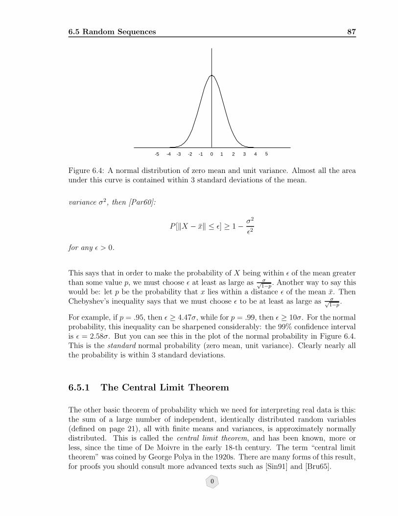
6.5 Random Sequences 87
-5 -4 -3 -1 1 2 3 4 5 -2 0
Figure 6.4: A normal distribution of zero mean and unit variance. Almost all the areaunder this curve is contained within 3 standard deviations of the mean.
variance σ2, then [Par60]:
P [‖X − x‖ ≤ ε] ≥ 1− σ2
ε2
for any ε > 0.
This says that in order to make the probability of X being within ε of the mean greaterthan some value p, we must choose ε at least as large as σ√
1−p . Another way to say thiswould be: let p be the probability that x lies within a distance ε of the mean x. ThenChebyshev’s inequality says that we must choose ε to be at least as large as σ√
1−p .
For example, if p = .95, then ε ≥ 4.47σ, while for p = .99, then ε ≥ 10σ. For the normalprobability, this inequality can be sharpened considerably: the 99% confidence intervalis ε = 2.58σ. But you can see this in the plot of the normal probability in Figure 6.4.This is the standard normal probability (zero mean, unit variance). Clearly nearly allthe probability is within 3 standard deviations.
6.5.1 The Central Limit Theorem
The other basic theorem of probability which we need for interpreting real data is this:the sum of a large number of independent, identically distributed random variables(defined on page 21), all with finite means and variances, is approximately normallydistributed. This is called the central limit theorem, and has been known, more orless, since the time of De Moivre in the early 18-th century. The term “central limittheorem” was coined by George Polya in the 1920s. There are many forms of this result,for proofs you should consult more advanced texts such as [Sin91] and [Bru65].
0

88 A Summary of Probability and Statistics
123456789101112131415161718192021222324252627282930313233343536373839404142434445464748495051525354555657585960616263646566676869707172737475767778798081828384858687888990919293949596979899100
0.02
0.04
0.06
0.08
123456789101112131415161718192021222324252627282930313233343536373839404142434445464748495051525354555657585960616263646566676869707172737475767778798081828384858687888990919293949596979899100
0.02
0.04
0.06
0.08
0.1
123456789101112131415161718192021222324252627282930313233343536373839404142434445464748495051525354555657585960616263646566676869707172737475767778798081828384858687888990919293949596979899100
0.02
0.04
0.06
0.08
0 50 100 0 50 100 0 50 100
100 Trials 1000 Trials 10000 Trials
Figure 6.5: Ouput from the coin-flipping program. The histograms show the outcomesof a calculation simulating the repeated flipping of a fair coin. The histograms havebeen normalized by the number of trials, so what we are actually plotting is the relativeprobability of of flipping k heads out of 100. The central limit theorem guarantees thatthis curve has a Gaussian shape, even though the underlying probability of the randomvariable is not Gaussian.
Theorem 11 Central Limit Theorem: If x is the sample mean of a sample of size nfrom a population with mean µ and standard deviation σ, then for any real numbers aand b with a < b
P
[µ+
aσ√n< x < µ+
bσ√n
]→ 1√
2π
∫ b
ae−z
2/2dz.
This just says that the sample mean is approximately normally distributed.
Since the central limit theorem says nothing about the particular distribution involved,it must apply to even something as apparently non-Gaussian as flipping a coin. Supposewe flip a fair coin 100 times and record the number of heads which appear. Now, repeatthe experiment a large number of times, keeping track of how many times there were 0heads, 1, 2, and so on up to 100 heads. Obviously if the coin is fair, we expect 50 headsto be the peak of the resulting histogram. But what the central limit theorem says isthat the curve will be a Gaussian centered on 50.
This is illustrated in Figure 6.5 via a little code that flips coins for us. For comparison,the exact probability of flipping precisely 50 heads is
100!
50!50!
(1
2
)100
≈ .076. (6.48)
What is the relevance of the Central Limit Theorem to real data? Here are threeconflicting views quoted in [Bra90]. From Scarborough (1966): “The truth is that, forthe kinds of errors considered in this book (errors of measurement and observation),the Normal Law is proved by experience. Several substitutes for this law have beenproposed, but none fits the facts as well as it does.”
From Press et al. (1986): “This infatuation [of statisticians with Gaussian statistics]tended to focus interest away from the fact that, for real data, the normal distribution
0

6.6 Expectations and Variances 89
is often rather poorly realized, if it is realized at all.”
And perhaps the best summary of all, Gabriel Lippmann speaking to Henri Poincare:“Everybody believes the [normal law] of errors: the experimenters because they believethat it can be proved by mathematics, and the mathematicians because they believe ithas been established by observation.”
6.6 Expectations and Variances
Notation: we use E[x] to denote the expectation of a random variable with respect toits probability law f(x). Sometimes it is useful to write this as Ef [x] if we are dealingwith several probability laws at the same time.
If the probability is discrete then
E[x] =∑
i
xif(xi).
If the probability is continuous then
E[x] =∫ ∞
−∞xf(x) dx.
Mixed probabilities (partly discrete, partly continuous) can be handled in a similar wayusing Stieltjes integrals [Bar76].
We can also compute the expectation of functions of random variables:
E[φ(x)] =∫ ∞
−∞φ(x)f(x) dx.
It will be left as an exercise to show that the expectation of a constant a is a (E[a] = a)and the expectation of a constant a times a random variable x is a times the expectationof x (E[ax] = aE[x]).
Recall that the variance of x is defined to be
V (x) = E[(x− E(x))2] = E[(x− µ)2]
where µ = E[x].
Here is an important result for expectations: E[(x − µ)2] = E[x2] − µ2. The proof iseasy.
E[(x− µ)2] = E[x2 − 2xµ+ µ2] (6.49)
= E[x2]− 2µE[x] + µ2 (6.50)
= E[x2]− 2µ2 + µ2 (6.51)
= E[x2]− µ2 (6.52)
0
90 A Summary of Probability and Statistics
An important result that we need is the variance of a sample mean. For this we usethe following lemma, the proof of which will be left as an exercise:
Lemma 1 If a is a real number and x a random variable, then V (ax) = a2V (x).
From this it follows immediately that
V (x) =1
n2
n∑
i=1
V (xi).
In particular, if the random variables are identically distributed, with mean µ thenV (x) = σ2/n.
6.7 Bias
In statistics, the bias of an estimator of some parameter is defined to be the expectationof the difference between the parameter and the estimator:
B[θ] ≡ E[θ − θ] (6.53)
where θ is the estimator of θ. In a sense, we want the bias to be small so that we havea faithful estimate of the quantity of interest.
An estimator θ of θ is unbiased if E[θ] = θ
For instance, it follows from the law of large numbers that the sample mean is anunbiased estimator of the population mean. In symbols,
E[x] = µ. (6.54)
However, the sample variance
s2 ≡ 1
N
N∑
i=1
(xi − x)2 (6.55)
turns out not to be unbiased (except asymptotically) since E[s2] = n−1nσ2. To get an
unbiased estimator of the variance we use E[ nn−1
s2]. To see this note that
s2 =1
N
n∑
i=1
(xi − x)2 =1
N
∑
i=1
x2i − 2xix + x2 =
(1
N
n∑
i=1
x2i
)− x2.
Hence the expected value of s2 is
E[s2] =1
N
n∑
i=1
E[x2i ]− E[x2].
0
6.7 Bias 91
Using a previous result, for each of the identically distributed xi we have
E[x2i ] = V (x) + E[x]2 = σ2 + µ2.
And
E[x2] = V (x) + E[x]2 =1
nσ2 + µ2.
So
E[s2] = σ2 + µ2 − 1
nσ2 − µ2 =
n− 1
nσ2.
Finally, there is the notion of the consistency of an estimator. An estimator θ of θ isconsistent if for every ε > 0
P [|θ − θ| < ε]→ 1 as n→∞.
Consistency just means that if the sample size is large enough, the estimator will beclose to the thing being estimated.
Later on, when we talk about inverse problems we will see that bias represents a po-tentially significant component of the uncertainty in the results of the calculations.Since the bias depends on something we do not know, the true value of the unknownparameter, it will be necessary to use a priori information in order to estimate it.
Mean-squared error, bias and variance
The mean-squared error (MSE) for an estimator m of mT is defined to be
MSE(m) ≡ E[(m−mT )2] = E[m2 − 2mmT +m2T ] = m2 − 2mmT +m2
T . (6.56)
By doing a similar analysis of the variance and bias we have:
Bias(m) ≡ E[m−mT ] = m−mT (6.57)
andVar(m) ≡ E[(m− m)2] = E[m2 − 2mm+ m2] = m2 − m2. (6.58)
So you can see that we have: MSE = Var + Bias2. As you can see, for a given mean-squared error, there is a trade-off between variance and bias. The following exampleillustrates this trade-off.
Example: Estimating the derivative of a smooth function
We start with a simple example to illustrate the effects of noise and prior information inthe performance of an estimator. Later we will introduce tools from statistical decisiontheory to study the performance of estimators given different types of prior information.
0
92 A Summary of Probability and Statistics
Suppose we have noisy observations of a smooth function, f , at the equidistant pointsa ≤ x1 ≤ . . . ≤ xn ≤ b
yi = f(xi) + εi, i = 1, ..., n, (6.59)
where the errors, εi, are assumed to be iid N(0, σ2)b. We want to use these observationsto estimate the derivative, f ′. We define the estimator
f ′(xmi) =yi+1 − yi
h, (6.60)
where h is the distance between consecutive points, and xmi = (xi+1+xi)/2. To measurethe performance of the estimator (6.60) we use the mean square error (MSE), which isthe sum of the variance and squared bias. The variance and bias of (6.60) are
Var[f ′(xmi)] =Var(yi+1) + Var(yi)
h2=
2σ2
h2,
Bias[f ′(xmi)] ≡ E[f ′(xmi)− f ′(xmi)]
=f(xi+1)− f(xi)
h− f ′(xmi) = f ′(αi)− f ′(xmi),
for some αi ∈ [xi, xi+1] (by the mean value theorem) . We need some information on f ′
to assess the size of the bias. Let us assume that the second derivative is bounded on[a, b] by M
|f ′′(x)| ≤M, x ∈ [a, b].
It then follows that
|Bias[f ′(xmi)]| = |f ′(αi)− f ′(xmi)| = |f ′′(βi)(αi − βi)| ≤Mh,
for some βi between αi and xmi . As h→ 0 the variance goes to infinity while the biasgoes to zero. The MSE is bounded by
2σ2
h2≤ MSE[f ′(xmi)] = Var[f ′(xmi)] + Bias[f ′(xmi)]
2 ≤ 2σ2
h2+M2h2. (6.61)
It is clear that choosing the smallest h possible does not lead to the best estimate;the noise has to be taken into account. The lowest upper bound is obtained with
h = 21/4√σ/M . The larger the variance of the noise, the wider the spacing between
the points.
We have used a bound on the second derivative to bound the MSE. It is a fact that sometype of prior information, in addition to model (6.59), is required to bound derivativeuncertainties. Take any smooth function, g, which vanishes at the points x1, ..., xn.Then, the function f = f + g satisfies the same model as f , yet their derivatives couldbe very different. For example, choose an integer, m, and define
g(x) = sin
[2πm(x− x1)
h
].
bIndependent, identically distributed random variables, normally distributed with mean 0 and vari-ance σ2.
0

6.8 Correlation of Sequences 93
Then, f(xi) + g(xi) = f(xi) and
f ′(x) = f ′(x) +2πm
hcos
[2πm(x− x1)
h
].
By choosing m large enough, we can make the difference, f ′(xmi) − f ′(xmi), as largeas we want; without prior information the derivative can not be estimated with finiteuncertainty.
6.8 Correlation of Sequences
Many people think that “random” and uncorrelated are the same thing. Randomsequences need not be uncorrelated. Correlation of sequences is measured by looking atthe correlation of the sequence with itself, the autocorrelation.c If this is approximatelya δ-function, then the sequence is uncorrelated. In a sense, this means that the sequencedoes not resemble itself for any lag other than zero. But suppose we took a deterministicfunction, such as sin(x), and added small (compared to 1) random perturbations to it.The result would have the large-scale structure of sin(x) but with a lot of random junksuperimposed. The result is surely still random, even though it will not be uncorrelated.
If the autocorrelation is not a δ-function, then the sequence is correlated. Figure 6.6shows two pseudo-random Gaussian sequences with approximately the same mean,standard deviation and 1D distributions: they look rather different. In the middle ofthis figure are shown the autocorrelations of these two sequences. Since the autocor-relation of the right-hand sequence drops off to approximately zero in 10 samples, wesay the correlation length of this sequence is 10. In the special case that the autocorre-lation of a sequence is an exponential function, the the correlation length is defined asthe (reciprocal) exponent of the best-fitting exponential curve. In other words, if theautocorrelation can be fit with an exponential e−z/`, then the best-fitting value of ` isthe correlation length. If the autocorrelation is not an exponential, then the correlationlength is more difficult to define. We could say that it is the number of lags of theautocorrelation within which the autocorrelation has most of its energy. It is oftenimpossible to define meaningful correlation lengths from real data.
A simple way to generate a correlated sequence is to take an uncorrelated one (this iswhat pseudo-random number generators produce) and apply some operator that cor-relates the samples. We could, for example, run a length-` smoothing filter over theuncorrelated samples. The result would be a series with a correlation length approxi-mately equal to `. A fancier approach would be to build an analytic covariance matrixand impose it on an uncorrelated pseudo-random sample.
cFrom the convolution theorem, it follows that the autocorrelation is just the inverse Fourier trans-form of the periodogram (absolute value squared of the Fourier transform).
0
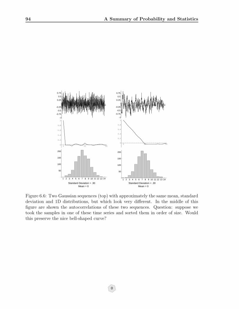
94 A Summary of Probability and Statistics
200 400 600 800 1000
-1
-0.75
-0.5
-0.25
0.25
0.5
0.75
200 400 600 800 1000
-1
-0.75
-0.5
-0.25
0.25
0.5
0.75
Standard Deviation = .30 Mean = 0 Mean = 0
1 2 3 4 5 6 7 8 9 10 11 12 13 14
50
100
150
200
1 2 3 4 5 6 7 8 9 10 11 12 13 14
50
100
150
200
Standard Deviation = .30
0 10 200
0.2
0.4
0.6
0.8
1
0 10 200
0.2
0.4
0.6
0.8
1
Figure 6.6: Two Gaussian sequences (top) with approximately the same mean, standarddeviation and 1D distributions, but which look very different. In the middle of thisfigure are shown the autocorrelations of these two sequences. Question: suppose wetook the samples in one of these time series and sorted them in order of size. Wouldthis preserve the nice bell-shaped curve?
0

6.8 Correlation of Sequences 95
For example, an exponential covariance matrix could be defined by Ci,j = σ2e−‖i−j‖/`
where σ2 is the (in this example) constant variance and ` is the correlation length.To impose this correlation on an uncorrelated, Gaussian sequence, we do a Choleskydecomposition of the covariance matrix and dot the lower triangular part into theuncorrelated sequence [Par94]. If A is a symmetric matrix, then we can always write
A = LLT ,
where L is lower triangular [GvL83]. This is called the Cholesky decomposition ofthe matrix A. You can think of the Cholesky decomposition as being somewhat likethe square root of the matrix. Now suppose we apply this to the covariance matrixC = LLT . Let x be a mean zero pseudo-random vector whose covariance is the identity.We will use L to transform x: z ≡ Lx. The covariance of z is given by
Cov(z) = E[zzT ] = E[(Lx)(Lx)T ] = LE[xxT ]LT = LILT = C
which is what we wanted.
Here is a simple Scilab code that builds an exponential covariance matrix Ci,j =σ2e−‖i−j‖/l and then returns n pseudo-random samples drawn from a Gaussian pro-cess with this covariance (and mean zero).
function [z] = correlatedgaussian(n,s,l)
// returns n samples of an exponentially correlated gaussian process
// with variance s^2 and correlation length l.
// first build the covariance matrix.
C = zeros(n,n);
for i = 1:n
for j = 1:n
C(i,j) = s^2 * exp(-abs(i-j)/l);
end
end
L = chol(C);
x = rand(n,1,’normal’);
z = L*x;
We would call this, for example, by:
z = correlatedgaussian(200,1,10);
0

96 A Summary of Probability and Statistics
The vector z should now have a standard deviation of approximately 1 and a correlationlength of 10. To see the autocorrelation of the vector you could do:
plot(corr(z,200))
the autocorrelation function will be approximately exponential for short lags. For longerlags you will see oscillatory departures from exponential behavior—even though thesamples are drawn from an analytic exponential covariance. This is due to the smallnumber of realizations. From the exponential part of the autocorrelation you can esti-mate the correlation length by simply looking for the point at which the autocorrelationhas decayed by 1/e. Or you can fit the log of the autocorrelation with a straight line.
6.9 Random Fields
If we were to make N measurements of, say, the density of a substance, we could plotthese N data as a function of the sample number. This plot might look somethinglike the top left curve in Figure 6.6. But these are N measurements of the same thing,unless we belive that the density of the sample is changing with time. So a histogram ofthe measurements would approximate the probability density function of the parameterand that would be the end of the story.
On the other hand, curves such as those in Figure 6.6 might result from measuring arandom, time-varying process. For instance, these might be measurements of a noisyaccelerometer, in which case the plot would be N samples of voltage versus time. Butthen these would not be N measurements of the same parameter, rather they wouldconstitute a single measurement of a random function of time, sampled at N times.The distinction we are making here is the distinction between a scalar-valued randomprocess and a random function. Now when we measure a function we always measureit at a finite number of locations (in space or time). So our measurements of randomfunction result in finite-dimensional random vectors. This is why the sampling of atime series of voltage, say, at N times, is really the realization of an N -dimensionalrandom process. For such a process it is not sufficient to simply make a histogram ofthe samples. We need higher order characterizations of the probability law behind thetime-series in order to account for the correlations of the measured values. This is thestudy of random fields or stochastic processes.
A real-data example of measurements of a random field is shown in Figure 6.7. Thesetraces represent 38 realizations of a time series recorded in a random medium. In thiscase the randomness is spatial: each realization is made at a different location in themedium. But you could easily imagine the same situation arising with a temporalrandom process. For example, these could be measurements of wave propagation in amedium undergoing random fluctuations in time, such as the ocean or the atmosphere.
0

6.9 Random Fields 97
0
0.05
0.10
0.15
0.20
time
(ms)
10 20 30realization
Figure 6.7: 38 realizations of an ultrasonic wave propagation experiment in a spatiallyrandom medium. Each trace is one realization of an unknown random process U(t).
The study of random processes is both conceptually and notationally difficult. Thereare advanced mathematical books such as Pugachev’s Theory of Random Functions[Pug65] which explain the situation, but from a physical point of view, one of theclearest explanations is in the book Statistical Optics by Goodman [Goo00]. We willfollow his lead.
So let us assume that there is an underlying random process U(t) (or U(r) if we wantto think about spatial randomness, it doesn’t matter for our purposes), the probabilitylaw of which we do not know. The notation U(t) is used to represent the ensemble of allpossible outcomes of the random process along with their probabilities. Each outcomewould be a function of time, say u(t). It is as if t is an index and u labels the sampledescription space of the random process.
If we don’t know the probability law of the random process, perhaps it is possibleto nevertheless characterize U by means, covariances, that sort of thing. Here is thetheorem, which you can find in [Pug65]. To completely characterize the probability lawof a stochastic process we must know the joint probability distribution
ρU(u1, u2, . . . , un, . . . ; t1, t2, . . . , tn, . . .)
for all n, where u1 = u(t1), etc. Of course, in practice, we only make measurements ofU at a finite numer of samples, so in practice we must make due with the n− th orderρU .d Now, the first-order PDF (probability density function) is ρU (u; t). Knowing this
dIt is sometimes convenient to label the joint distribution by the random process, and sometimesby the order. So,
ρU (u1, u2, . . . , un; t1, t2, . . . , tn) ≡ ρn(u1, u2, . . . , un; t1, t2, . . . , tn)
0

98 A Summary of Probability and Statistics
we can compute E[u], E[u2], etc. The second-order PDF involves two times, t1 and t2,and is the joint PDF of U(t1) and U(t2): ρ2(u1, u2; t1, t2). With this we can computequantities such as:
E[u1u2] =∫ ∫
u1u2ρU (u1, u2; t1, t2)du1du2.
It is relatively uncommon to go beyond second order statistical characterizations (meansand covariances) and we will not do so in this class.
Time versus statistical autocorrelation
Given a known function u(t) (or this could be discrete samples of a known functionu(ti)), the time autocorrelation function of u is defined as:
Γu(τ) = limT←∞
1
T
∫ T/2
−T/2u(t+ τ)u(t)dt.
This measures the similarity of u(t+τ) and u(t) averaged over all time. Closely relatedis the statistical autocorrelation function. Let U(t) be a random process. Implicitythe random process consistutes the set of all possible sample functions u(t) and theirassociated probability measure.
Γu(t1, t2) ≡ E[u(t1)u(t2)] =∫ ∞
−∞
∫ ∞
−∞u2u1ρU(u1, u2; t1, t2)du1du2.
Γu(t1, t2) measures the statistical similarity of u(t1) and u(t2) over the ensemble of allpossible realizations of U(t).
For stationary processes, Γu(t1, t2) depends only on τ ≡ t2 − t1. And for ergodicprocesses:
Γ(τ) = Γu(τ)
6.10 Probabilistic Information About Earth Models
In geophysics there is a large amount of a priori information that could be used toinfluence inverse calculations. Here, a priori refers to the assumption that this infor-mation is known independently of the data. Plausible geologic models can be based onrock outcrops, models of sedimentological deposition, subsidence, etc. There are alsooften in situ and laboratory measurements of rock properties that have a direct bearingon macroscopic seismic observations, such as porosity, permeability, crack orientation,etc. There are other, less quantitative, forms of information as well, the knowledge ofexperts for instance.
This prior information can be deterministic or probabilistic. Examples of deterministicinformation include: density is positive, wave velocity is positive (and less than the
0
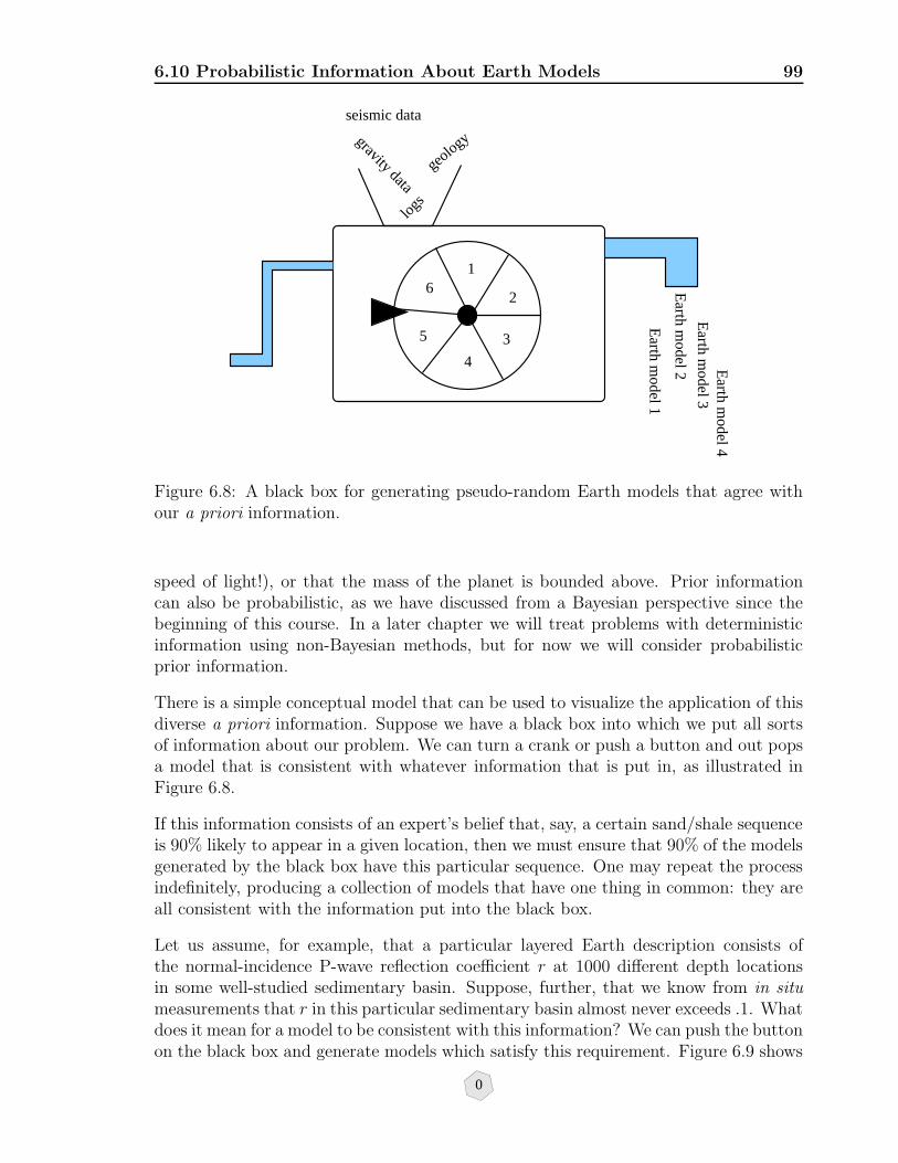
6.10 Probabilistic Information About Earth Models 99
1
3
4
5
6
logs
gravity datageo
logy
seismic data
2
Earth m
odel 2
Earth m
odel 3E
arth model 4
Earth m
odel 1
Figure 6.8: A black box for generating pseudo-random Earth models that agree withour a priori information.
speed of light!), or that the mass of the planet is bounded above. Prior informationcan also be probabilistic, as we have discussed from a Bayesian perspective since thebeginning of this course. In a later chapter we will treat problems with deterministicinformation using non-Bayesian methods, but for now we will consider probabilisticprior information.
There is a simple conceptual model that can be used to visualize the application of thisdiverse a priori information. Suppose we have a black box into which we put all sortsof information about our problem. We can turn a crank or push a button and out popsa model that is consistent with whatever information that is put in, as illustrated inFigure 6.8.
If this information consists of an expert’s belief that, say, a certain sand/shale sequenceis 90% likely to appear in a given location, then we must ensure that 90% of the modelsgenerated by the black box have this particular sequence. One may repeat the processindefinitely, producing a collection of models that have one thing in common: they areall consistent with the information put into the black box.
Let us assume, for example, that a particular layered Earth description consists ofthe normal-incidence P-wave reflection coefficient r at 1000 different depth locationsin some well-studied sedimentary basin. Suppose, further, that we know from in situmeasurements that r in this particular sedimentary basin almost never exceeds .1. Whatdoes it mean for a model to be consistent with this information? We can push the buttonon the black box and generate models which satisfy this requirement. Figure 6.9 shows
0
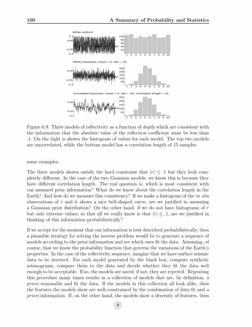
100 A Summary of Probability and Statistics
200 400 600 800 1000
-0.1
-0.05
0.05
0.1
200 400 600 800 1000
-0.1
-0.05
0.05
1 2 3 4 5 6 7 8 9 10
20
40
60
80
100
1 2 3 4 5 6 7 8 9 10
50
100
150
200
250
1 2 3 4 5 6 7 8 9 10
50
100
150
200
250
200 400 600 800 1000
-0.1
-0.05
0.05
White uniform
White Gaussian, mean = 0, std = .03
Correlated Gaussian, mean = 0, std = .03, correlation length = 15
Figure 6.9: Three models of reflectivity as a function of depth which are consistent withthe information that the absolute value of the reflection coefficient must be less than.1. On the right is shown the histogram of values for each model. The top two modelsare uncorrelated, while the bottom model has a correlation length of 15 samples.
some examples.
The three models shown satisfy the hard constraint that |r| ≤ .1 but they look com-pletely different. In the case of the two Gaussian models, we know this is because theyhave different correlation length. The real question is, which is most consistent withour assumed prior information? What do we know about the correlation length in theEarth? And how do we measure this consistency? If we make a histogram of the in situobservations of r and it shows a nice bell-shaped curve, are we justified in assuminga Gaussian prior distribution? On the other hand, if we do not have histograms of rbut only extreme values, so that all we really know is that |r| ≤ .1, are we justified inthinking of this information probabilistically?
If we accept for the moment that our information is best described probabilistically, thena plausible strategy for solving the inverse problem would be to generate a sequence ofmodels according to the prior information and see which ones fit the data. Assuming, ofcourse, that we know the probability function that governs the variations of the Earth’sproperties. In the case of the reflectivity sequence, imagine that we have surface seismicdata to be inverted. For each model generated by the black box, compute syntheticseismograms, compare them to the data and decide whether they fit the data wellenough to be acceptable. If so, the models are saved; if not, they are rejected. Repeatingthis procedure many times results in a collection of models that are, by definition, apriori reasonable and fit the data. If the models in this collection all look alike, thenthe features the models show are well-constrained by the combination of data fit and apriori information. If, on the other hand, the models show a diversity of features, then
0
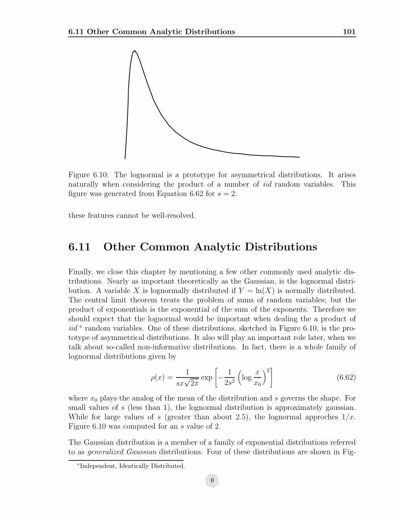
6.11 Other Common Analytic Distributions 101
Figure 6.10: The lognormal is a prototype for asymmetrical distributions. It arisesnaturally when considering the product of a number of iid random variables. Thisfigure was generated from Equation 6.62 for s = 2.
these features cannot be well-resolved.
6.11 Other Common Analytic Distributions
Finally, we close this chapter by mentioning a few other commonly used analytic dis-tributions. Nearly as important theoretically as the Gaussian, is the lognormal distri-bution. A variable X is lognormally distributed if Y = ln(X) is normally distributed.The central limit theorem treats the problem of sums of random variables; but theproduct of exponentials is the exponential of the sum of the exponents. Therefore weshould expect that the lognormal would be important when dealing the a product ofiid e random variables. One of these distributions, sketched in Figure 6.10, is the pro-totype of asymmetrical distributions. It also will play an important role later, when wetalk about so-called non-informative distributions. In fact, there is a whole family oflognormal distributions given by
ρ(x) =1
sx√
2πexp
[− 1
2s2
(log
x
x0
)2]
(6.62)
where x0 plays the analog of the mean of the distribution and s governs the shape. Forsmall values of s (less than 1), the lognormal distribution is approximately gaussian.While for large values of s (greater than about 2.5), the lognormal approches 1/x.Figure 6.10 was computed for an s value of 2.
The Gaussian distribution is a member of a family of exponential distributions referredto as generalized Gaussian distributions. Four of these distributions are shown in Fig-
eIndependent, Identically Distributed.
0
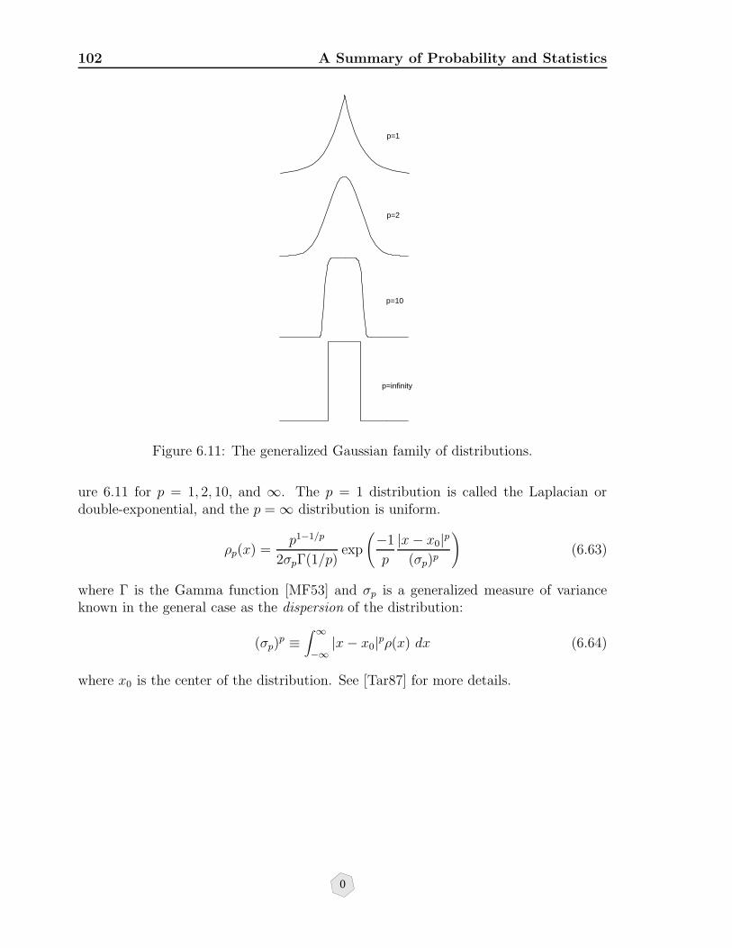
102 A Summary of Probability and Statistics
p=10
p=2
p=infinity
p=1
Figure 6.11: The generalized Gaussian family of distributions.
ure 6.11 for p = 1, 2, 10, and ∞. The p = 1 distribution is called the Laplacian ordouble-exponential, and the p =∞ distribution is uniform.
ρp(x) =p1−1/p
2σpΓ(1/p)exp
(−1
p
|x− x0|p(σp)p
)(6.63)
where Γ is the Gamma function [MF53] and σp is a generalized measure of varianceknown in the general case as the dispersion of the distribution:
(σp)p ≡
∫ ∞
−∞|x− x0|pρ(x) dx (6.64)
where x0 is the center of the distribution. See [Tar87] for more details.
0
6.11 Other Common Analytic Distributions 103
Exercises
1. Show that for any two events A and B
P (ABc) = P (A)− P (BA) (6.65)
2. Show that for any event A, P (Ac) = 1− P (A).
3. Show that 1/x is a measure, but not a probability density.
4. Show that the truth of the following formula for any two sets A and B
P (A ∪ B) = P (A) + P (B)− P (A ∪B) (6.66)
follows from the fact that for independent sets A′ and B′
P (A′ ∪ B′) = P (A′) + P (B′). (6.67)
Hint. The union of any two sets A and B can be written as the sum of threeindependent sets of elements: the elements in A but not in B; the elements in Bbut not in A; and the elements in both A and B.
5. Show that all the central moments of the normal distribution beyond the secondare either zero or can be written in terms of the mean and variance.
6. You have made n different measurements of the mass of an object. You wantto find the mass that best “fits” the data. Show that the mass estimator whichminimizes the sum of squared errors is given by the mean of the data, while themass estimator which minimizes the sum of the absolute values of the errors isgiven by the median of the data. Feel free to assume that you have an odd numberof data.
7. Show that Equation 6.47 is normalized.
8. Take the n data you recorded above and put them in numerical order: x1 ≤ x2 ≤... ≤ xn. Compute the sensitivity of the two different estimators, average andmedian, to perturbations in xn.
What does this say about how least squares and least absolute values treat “out-liers” in the data?
9. Find the normalization constant that will make
p(x) = e−(x2−x0x+x20) (6.68)
a probability density on the real line. x0 is a constant.
What are the mean and variance?
0
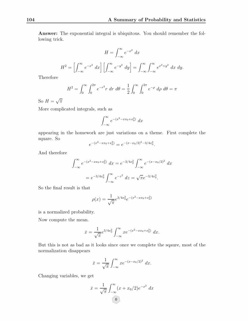
104 A Summary of Probability and Statistics
Answer: The exponential integral is ubiquitous. You should remember the fol-lowing trick.
H =∫ ∞
−∞e−x
2
dx
H2 =[∫ ∞
−∞e−x
2
dx] [∫ ∞
−∞e−y
2
dy]
=∫ ∞
−∞
∫ ∞
−∞ex
2+y2
dx dy.
Therefore
H2 =∫ ∞
0
∫ 2π
0e−r
2
r dr dθ =1
2
∫ ∞
0
∫ 2π
0e−ρ dρ dθ = π
So H =√π
More complicated integrals, such as∫ ∞
−∞e−(x2−xx0+x2
0) dx
appearing in the homework are just variations on a theme. First complete thesquare. So
e−(x2−xx0+x20) = e−(x−x0/2)2−3/4x2
0 .
And therefore∫ ∞
−∞e−(x2−xx0+x2
0) dx = e−3/4x20
∫ ∞
−∞e−(x−x0/2)2
dx
= e−3/4x20
∫ ∞
−∞e−z
2
dz =√πe−3/4x2
0 .
So the final result is that
ρ(x) =1√πe3/4x2
0e−(x2−xx0+x20)
is a normalized probability.
Now compute the mean.
x =1√πe3/4x2
0
∫ ∞
−∞xe−(x2−xx0+x2
0) dx.
But this is not as bad as it looks since once we complete the sqaure, most of thenormalization disappears
x =1√π
∫ ∞
−∞xe−(x−x0/2)2
dx.
Changing variables, we get
x =1√π
∫ ∞
−∞(x+ x0/2)e−x
2
dx
0

6.12 Computer Exercise 105
=1√π
∫ ∞
−∞xe−x
2
dx+1√πx0/2
∫ ∞
−∞e−x
2
dx.
The first integral is exactly zero, while the second (using our favorite formula) isjust x0/2, so x = x0/2.
Similarly, to compute the variance we need to do
σ2 =1√π
∫ ∞
−∞(x− x0/2)2e−(x−x0/2)2
dx =1√π
∫ ∞
−∞z2e−z
2
dz.
Anticipating an integration by parts, we can write this integral as
−1
2
∫ ∞
−∞zd(e−z
2)
=1
2
∫ ∞
−∞e−z
2
dz =1
2
√π
using, once again, the exponential integral result. So the variance is just 1/2.
some common exponential integrals[Dwi61]
∫ ∞
0e−r
2x2
dx =
√π
2rr > 0 throughout this box (6.69)
∫ ∞
0xe−r
2x2
dx =1
2r2(6.70)
∫ ∞
0x2a+1e−r
2x2
dx =a!
2r2a+2a = 1, 2, . . . (6.71)
∫ ∞
0x2ae−r
2x2
dx =1 · 3 · 5 · · · (2a− 1)
2a+1r2a+1
√π a = 1, 2, . . . (6.72)
Normal probability integral ≡ 1√2π
∫ x
−xe−t
2/2dt = erfx√2
(6.73)
Error function ≡ erfx ≡ 2√π
∫ x
0e−t
2/2dt =2x√π
[1− x2
1!3+x4
2!5− x6
3!7· · ·]
(6.74)
erfx ≈ 1− e−x2
x√π
[1− 2!
1!(2x)2+
4!
2!(2x)4+
6!
3!(2x)6· · ·]
(6.75)
6.12 Computer Exercise
Write a program that computes the sample covariance matrix of repeated recordings ofa time series. To test your code, generate 25 correlated time series of length 100 anduse these as data. In other words the sample size will be 25 and the covariance matrixwill be of order 100.
0

106 BIBLIOGRAPHY
Bibliography
[Bar76] R.G. Bartle. The Elements of Real Analysis. Wiley, 1976.
[Bra90] R. Branham. Scientific Data Analysis. Springer-Verlag, 1990.
[Bru65] H.D. Brunk. An Introduction to Mathematical Statistics. Blaisdell, 1965.
[Dwi61] H.B. Dwight. Tables of Integrals and Other Mathematical Data. MacmillanPublishers, 1961.
[Goo00] J.W. Goodman. Statistical Optics. Wiley, 2000.
[GvL83] G. Golub and C. van Loan. Matrix Computations. Johns Hopkins, Baltimore,1983.
[Knu81] D. Knuth. The Art of Computer Programming, Vol II. Addison Wesley, 1981.
[MF53] P.M. Morse and H. Feshbach. Methods of Theoretical Physics. McGraw Hill,1953.
[MGB74] A.M. Mood, F.A. Graybill, and D.C. Boes. Introduction to the Theory ofStatistics. McGraw-Hill, 1974.
[Par60] E. Parzen. Modern Probability Theory and its Applications. Wiley, 1960.
[Par94] R.L. Parker. Geophysical Inverse Theory. Princeton University Press, 1994.
[Pug65] S. Pugachev, V.˙ Theory of random functions and its application to controlproblems. Pergamon, 1965.
[Sin91] Y.G. Sinai. Probability Theory: and Introductory Course. Springer, 1991.
[Tar87] A. Tarantola. Inverse Problem Theory. Elsevier, New York, 1987.
0

Chapter 7
Linear Inverse Problems WithUncertain Data
In Chapter 5 we showed that the SVD could be used to solve a linear inverse problem inwhich the only uncertainties were associated with the data. The canonical formulationof such a problem is
d = Am + ε (7.1)
where it is assumed that the forward operator A is linear and exactly known andthat the uncertainties arise from additive noise in the data. In most geophysical inverseproblems, the vector m is properly defined in an infinite dimensional space of functions;for example, the elastic tensor as a function of space. As a practical matter the modelspace is usually discretized so that the problem is numerically finite dimensional. This isa potential source of error (bias, discretization error), but for now we will ignore this andassume that the discretization is very fine, but nevertheless finite. This is equivalent toassuming a priori that the true Earth model is confined to a finite dimensional subspaceof the model space.
If there are no discretization errors, and if the forward model is linear and known,then the observations d are the response of the true model mT under the action of A,provided there are no measurement or other systematic errors.
As defined in Section 6.5 m† is a pseudo-inverse estimator of the true model: thegeneralized solution of Equation 7.1 is given by m† = A†d. Since d is the response ofthe true model, mtrue, it follows that
m† ≡ A†d = A†(Amtrue + ε) = A†Amtrue + A†ε.
In terms of the SVD, the resolution matrix A†A can be written VrVTr and so represents
a projection operator onto the non-null space of the forward problem (i.e., the rowspace). Since none of the columns of Vr lie in the null space of A, the net result of this
1
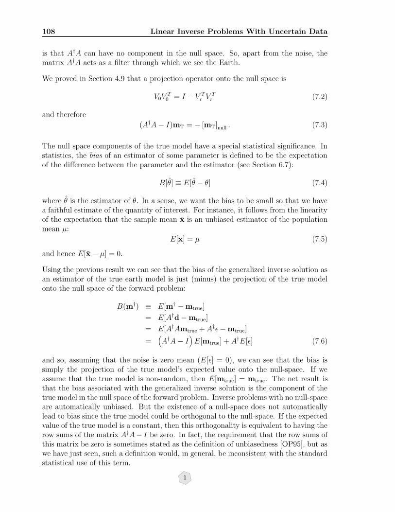
108 Linear Inverse Problems With Uncertain Data
is that A†A can have no component in the null space. So, apart from the noise, thematrix A†A acts as a filter through which we see the Earth.
We proved in Section 4.9 that a projection operator onto the null space is
V0VT
0 = I − V Tr V
Tr (7.2)
and therefore
(A†A− I)mT = − [mT]null . (7.3)
The null space components of the true model have a special statistical significance. Instatistics, the bias of an estimator of some parameter is defined to be the expectationof the difference between the parameter and the estimator (see Section 6.7):
B[θ] ≡ E[θ − θ] (7.4)
where θ is the estimator of θ. In a sense, we want the bias to be small so that we havea faithful estimate of the quantity of interest. For instance, it follows from the linearityof the expectation that the sample mean x is an unbiased estimator of the populationmean µ:
E[x] = µ (7.5)
and hence E[x− µ] = 0.
Using the previous result we can see that the bias of the generalized inverse solution asan estimator of the true earth model is just (minus) the projection of the true modelonto the null space of the forward problem:
B(m†) ≡ E[m† −mtrue]
= E[A†d−mtrue]
= E[A†Amtrue + A†ε−mtrue]
=(A†A− I
)E[mtrue] + A†E[ε] (7.6)
and so, assuming that the noise is zero mean (E[ε] = 0), we can see that the bias issimply the projection of the true model’s expected value onto the null-space. If weassume that the true model is non-random, then E[mtrue] = mtrue. The net result isthat the bias associated with the generalized inverse solution is the component of thetrue model in the null space of the forward problem. Inverse problems with no null-spaceare automatically unbiased. But the existence of a null-space does not automaticallylead to bias since the true model could be orthogonal to the null-space. If the expectedvalue of the true model is a constant, then this orthogonality is equivalent to having therow sums of the matrix A†A− I be zero. In fact, the requirement that the row sums ofthis matrix be zero is sometimes stated as the definition of unbiasedness [OP95], but aswe have just seen, such a definition would, in general, be inconsistent with the standardstatistical use of this term.
1

7.1 The World’s Second Smallest Inverse Problem 109
7.0.1 Model Covariances
Estimators are functions of the data and therefore random variables. The covarianceof a random variable x is the second central moment:
C = E[(x− E[x])(x− E[x])T ]. (7.7)
The covariance of the generalized inverse estimate m† ≡ A†d is easy to compute. Firstrealize that if d has zero mean than so does m† a and therefore assuming zero meanerrors
Cov(m) = E[m†m†T
] = A†Cov(d)A†T
(7.8)
If the data are uncorrelated, then Cov(d) is a diagonal matrix whose elements are thestandard deviations of the data. If we go one step further and assume that all thesestandard deviations are the same, σ2
d,b then the covariance of the generalized inverse
estimate takes on an especially simple form:
Cov(m†) = σ2dA†A† = σ2
dVrΛ−2r V T
r .
We can see that the uncertainties in the estimated model parameters (expressed asCov(δm†)) are proportional to the data uncertainties and inversely proportional tothe squared singular values. This is as one would expect: as the noise increases, theuncertainty in our parameter estimates increases; and further, the parameters associatedwith the smallest singular values will be less well resolved than those associated withthe largest.
7.1 The World’s Second Smallest Inverse Problem
Suppose we wanted to use sound to discover the depth to bedrock below our feet. Wecould set off a loud bang at the surface and wait to see how long it would take for theecho from the top of the bedrock to return to the surface. Then, assuming that thegeologic layers are horizontal, can we compute the depth to bedrock z from the traveltime of the reflected bang t? Suppose we do not know the speed with which soundspropagates beneath us, so that all we can say is that the travel time must depend bothon this speed and on the unknown depth
t = 2z/c.
Since this toy problem involves many of the complications of more realistic inversecalculations, it will be useful to go through the steps of setting up and solving thecalculation. We can absorb the factor of two into a new sound speed c and write
t = z/c. (7.9)
aWhy? since m† = A†, E[m†] = A†E[d].bI.e., assume that the data are iid with mean zero and standard deviation σd.
1

110 Linear Inverse Problems With Uncertain Data
So the model vector m is (z, c) since c and z are both unknown, and the data vector dis simply t. The forward problem is g(m) = z/c. Notice that g is linear in depth, butnonlinear in sound speed c. We can linearize the forward problem by doing a Taylorseries expansion about some model (z0, c0) and retaining only the first order term:
t = t0 +z0
c0
[1
z0,− 1
c0
] [δzδc
](7.10)
where t0 = z0/c0. Pulling the t0 over to the left side and diving by t0 we have
δt
t0= [1,−1]
[δzz0δcc0
](7.11)
In this particular case the linearization is independent of the starting model (z0, c0)since by computing the total derivative of of t we get
δt
t=δz
z− δc
c. (7.12)
In other words, by defining new parameters to be the logarithms of the old parameters,or the dimensionless perturbations, (but keeping the same symbols for convenience) wehave
t = z − c. (7.13)
In any case, the linear(-ized) forward operator is the 1× 2 matrix A = (1,−1) and
ATA =
[1 −1−1 1
]. (7.14)
Let’s work out the SVD of A by hand. First, let us make the convention that modelvectors and data vectors are column vectors. We could make them row vectors too, butwe must keep to some convention in order to avoid getting confused. So
The forward operator matrix A must be a 1 by 2 matrix
A = [1 − 1]
since d ∈ R1 and m ∈ R2. Therefore
ATA =
[1−1
][1 − 1] =
[1 −1−1 1
]
and
AAT = [1 − 1]
[1−1
]= 2.
So the eigenvalue of a 1 × 1 matrix (a scalar) is just this number. The eigenvalues ofAAT are the squares of the singular values, so the one and only non-zero singular valueis√
2.
1

7.1 The World’s Second Smallest Inverse Problem 111
Now since the data space is one-dimensional, the data-space eigenvector is just a nor-malized vector in R1–which is just 1. So Ur = 1. To get Vr we don’t even need ATAsince we know that
ATUr = VrΛr.
So [1−1
]· 1 =
√2Vr ⇒ Vr =
1√2
[1−1
].
The complete SVD then is
A = 1 ·√
2 · 1√2
[1−1
]T= 1 ·
√2 · 1√
2[1 − 1] .
where Ur = 1, Λr =√
2, and Vr = 1/√
2[1 − 1]T .
So, the eigenvalues of ATA are 2 and 0. 2 is the eigenvalue of the (unnormalized)eigenvector (1,−1)T , while 0 is the eigenvalue of (1, 1)T . The latter follows from thefact that AV0 = 0 so
[1 − 1]
[v0
v1
]= 0⇒ V0 =
[11
]
This has a simple physical interpretation. An out-of-phase perturbation of velocityand depth (increase one and decrease the other) changes the travel time, while an inphase perturbation (increase both) does not. Since an in phase perturbation must beproportional to (1, 1)T , it stands to reason that this vector would be in the null spaceof A. But notice that we have made this physical argument without reference to thelinearized (log parameter) problem. However, since we spoke in terms of perturbationsto the model, the assumption of a linear problem was implicit. In other words, bythinking of the physics of the problem we were able to guess the singular vectors of thelinearized problem without even considering the linearization explicitly.
In the notation we developed for the SVD, we can say that Vr, the matrix of non-null-space model singular vectors is (1,−1)T , while V0, the matrix of null-space singularvectors is (1, 1)T . And hence, using the normalized singular vectors, the resolutionoperator is
VrVTr =
1√2
[1 −1−1 1
]. (7.15)
The covariance matrix of the depth/velocity model is
A†Cov(d)A†T = σ2A†A†T (7.16)
assuming the single travel time datum has normally distributed error. Hence the co-variance matrix is
Cov(m) =(σ
2
)2[
1 −1−1 1
]. (7.17)
1

112 Linear Inverse Problems With Uncertain Data
The important thing to notice here is that this says the velocity and depth are com-pletely correlated (off diagonal entries magnitude equal to 1), and that the correlationis negative. This means that increasing one is the same as decreasing the other. Thecovariance matrix itself has the following eigenvalue/eigenvector decomposition.
Cov(m) =(σ
2
)2[
1 1−1 1
] [1 00 0
] [1 −11 1
]. (7.18)
These orthogonal matrices correspond to rotations of the velocity/depth axes. Theseaxes are associated with the line z/c = t. So for a given travel time t, we can beanywhere on the line z = tc: there is complete uncertainty in model space along thisline and this uncertainty is reflected in the zero eigenvalue of the covariance matrix.
For a two-dimensional problem such as this the correlation coefficient measures the sim-ilarity in the fluctuations in the two random variables. Here the two random variablesare our estimates of z and c. Formally the correlation coefficient is defined to be:
r =Czcσzσc
.
Since the covariance matrix is symmetric Czc = Ccz. σz and σc are just the standarddeviations of the corresponding parameter estimates: σz =
√Czz and σc =
√Ccc. So
r =−1
1.
It is not hard to show that for a two-dimensional Gaussian probability density, thelevel surfaces (contours of constant probability) are ellipses (circles and lines beingspecial cases of ellipses). If the two random variables are zero-mean and have the samevariances, then the level surfaces fall into one of three classes depending on the sizeof the correlation coefficient. First note that the correlation coefficient is always lessthan or equal to one in absolute value. If r = 0 then the level surfaces are circles. If0 < |r| < 1, then the level surfaces are true ellipses. Finally, if |r| = 1 the level surfacesare lines, as in the example above.
7.1.1 The Damped Least Squares Problem
The generalized inverse solution of the two-parameter problem is
m† = A†t =t
2
[1−1
]. (7.19)
As we have seen before, least squares tends to want to average over ignorance. Sincewe cannot determine velocity and depth individually, but only their ratio, least squaresputs half the data into each. Damping does not change this, it is still least squares, butit does change the magnitude of the computed solution. Since damping penalizes the
1
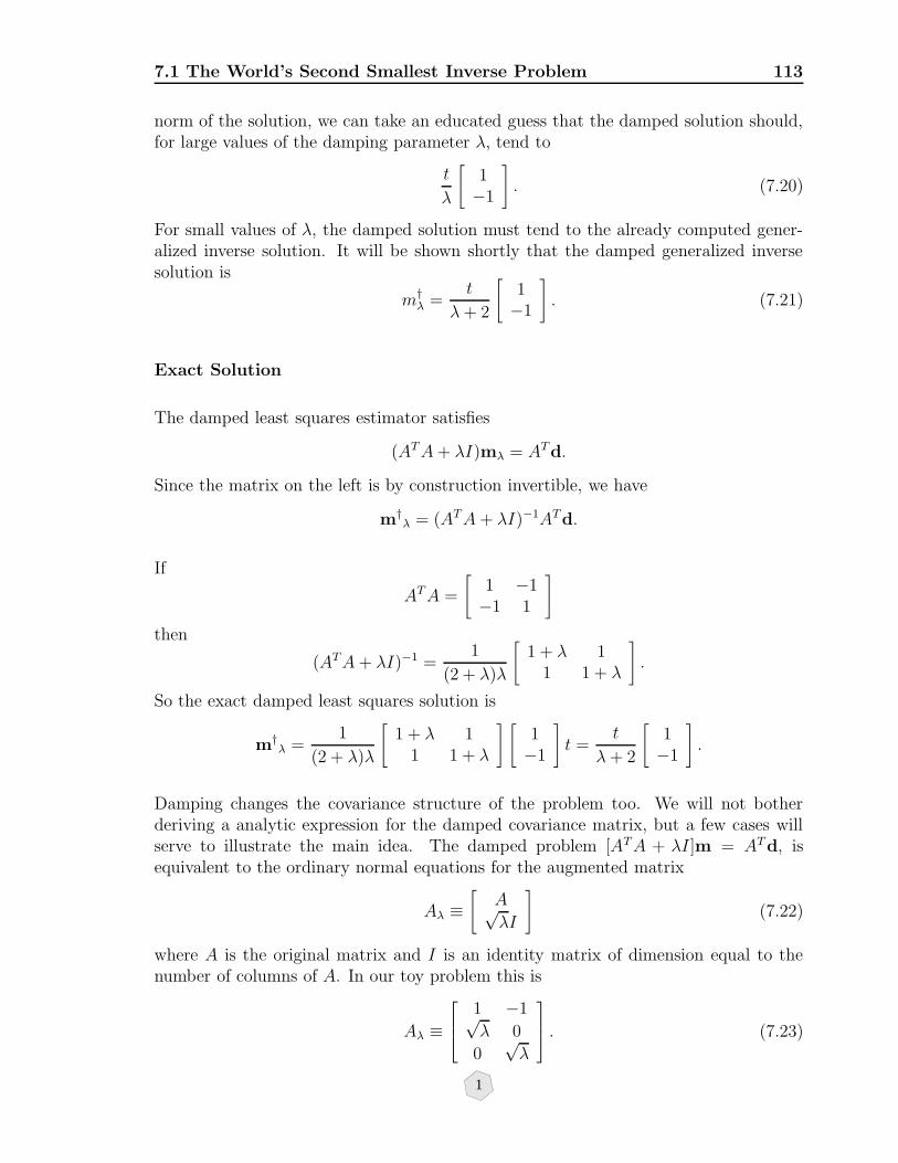
7.1 The World’s Second Smallest Inverse Problem 113
norm of the solution, we can take an educated guess that the damped solution should,for large values of the damping parameter λ, tend to
t
λ
[1−1
]. (7.20)
For small values of λ, the damped solution must tend to the already computed gener-alized inverse solution. It will be shown shortly that the damped generalized inversesolution is
m†λ =t
λ+ 2
[1−1
]. (7.21)
Exact Solution
The damped least squares estimator satisfies
(ATA+ λI)mλ = ATd.
Since the matrix on the left is by construction invertible, we have
m†λ = (ATA + λI)−1ATd.
If
ATA =
[1 −1−1 1
]
then
(ATA+ λI)−1 =1
(2 + λ)λ
[1 + λ 1
1 1 + λ
].
So the exact damped least squares solution is
m†λ =1
(2 + λ)λ
[1 + λ 1
1 1 + λ
] [1−1
]t =
t
λ+ 2
[1−1
].
Damping changes the covariance structure of the problem too. We will not botherderiving a analytic expression for the damped covariance matrix, but a few cases willserve to illustrate the main idea. The damped problem [ATA + λI]m = ATd, isequivalent to the ordinary normal equations for the augmented matrix
Aλ ≡[
A√λI
](7.22)
where A is the original matrix and I is an identity matrix of dimension equal to thenumber of columns of A. In our toy problem this is
Aλ ≡
1 −1√λ 0
0√λ
. (7.23)
1

114 Linear Inverse Problems With Uncertain Data
The covariance matrix for the augmented system is
Cov(m) = A†λCov(d)A†Tλ . (7.24)
For example, with λ = 1 the velocity/depth covariance is
Cov(z, c) =σ2
3
[2 11 2
]. (7.25)
Right away we can see that since the eigenvalues of this matrix are 1 and 3, instead ofa degenerate ellipsoid (infinite aspect ratio), the error ellipsoid of the damped problemhas an aspect ratio of 3. As the damping increases, the covariance matrix becomesincreasingly diagonal, resulting in a circular error ellipsoid. You will calculate theanalytic result as an exercise. Your result should become degenerate as λ→ 0.
Exercises
• Extend the two-parameter travel time inversion problem to the case in whichthe ray reflects from the flat interface at an angle of θ, measured relative to thevertical. I.e, θ = 0 would correspond to a ray that goes straight up and down.Assume that the travel time can be measured with an uncertainty of σ second.
• Compute the pseudoinverse and resolution matrix of(
1 −1 2 04 −4 0 0
)
Assuming the right hand side is (0, 1)T , what is the least squares estimator of the4-dimensional model vector.
• Compute the pseudoinverse and resolution matrix of
1. −14 −40 10 −1
Assuming the right hand side is (0, 1,−1, 0)T , what is the least squares estimatorof the 4-dimensional model vector.
• Assuming the data covariance matrix is
1 0 0 00 .5 0 00 0 .1 00 0 0 .0001
compute the covariance of matrix of the least squares estimator.
1

BIBLIOGRAPHY 115
• Find the inverse of the covariance matrix in Equation 7.25. Now see if you canfind the square root of this matrix. I.e., a matrix such that when you square it,you get the inverse of the covariance matrix.
• Compute the exact covariance and resolution for the damped two-parameter prob-lem.
Bibliography
[OP95] J. Ory and R. Pratt. Are our parameter estimators biased? the significance offinite-difference regularization operators. Inverse Problems, 11:397–424, 1995.
1

116 BIBLIOGRAPHY
1
Chapter 8
Examples: Absorption and TravelTime Tomography
Before we go any further, it will be useful to motivate all the work we’re doing with anexample that is sufficiently simple that we can do all the calculations without too muchstress. We will consider and example of “tomography”. The word tomography comesfrom the Greek tomos meaning section or slice. The idea is to use observed values ofsome quantity which is related via a line integral to the physical parameter we wish toinfer. Here we will study seismic travel time tomography, is is a widely used method ofimaging the earth’s interior. Mathematically this problem is identical to other types oftomography such as used in X-ray CAT scans.
8.1 The X-ray Absorber
Most of the examples shown here are based on an idealized two-dimensional x-rayabsorption experiment. This experiment consists of the measurement of the power lossof x-ray beams passing through a domain filled with an x-ray absorber.
We suppose that the absorber is confined to the unit square,
(x, y) ∈ [0, 1] ⊗ [0, 1];
we will represent this domain by DX. We also suppose that the sensing beam followsa perfectly straight path from transmitter to receiver and that the transmitter andreceiver are located on the perimeter of the unit square. The geometry of a single x-rayabsorption measurement looks like Figure 8.1.
1

118 Tomography
transmitter
receiver
Figure 8.1: An x-ray source shoots x-rays across a target to a detector where theintensity (energy) of the beam is measured.
8.1.1 The Forward Problem
Let c(x, y) be the absorption coefficient in DX; we assume that c(x, y) is non-negativeeverywhere. Let IT be the emitted beam intensity from a transmitter, T ; and let IR bethe received intensity at some receiver, R. Then the absorption law is exactly
IR = IT e−∫ TRc(x,y)dλ (8.1)
where the integral is along the (perfectly straight) path from T to R and dλ is arc-lengthalong the path. (Note that c(x, y) = 0 in a vacuum and the exponent in equation (8.1)vanishes.)
It is convenient to replace intensities with
ρ =IT − IR
IT, (8.2)
which is just the fractional intensity drop. ρ has the virtues that
• ρ is independent of transmitter strength, IT ,
• ρ = 0 for a beam which passes only through a vacuum,
• ρ ≥ 0 for all reasonable mediaa and, in fact, 0 ≤ ρ < 1, if c(x, y) is everywherenon-negative and finite.
aA “reasonable” medium is one which does not add energy to beams passing through. A laser isnot a reasonable medium.
1
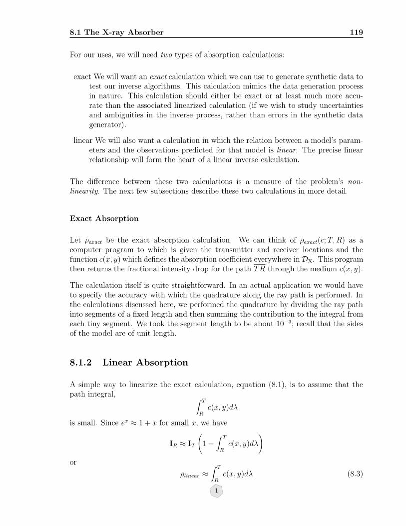
8.1 The X-ray Absorber 119
For our uses, we will need two types of absorption calculations:
exact We will want an exact calculation which we can use to generate synthetic data totest our inverse algorithms. This calculation mimics the data generation processin nature. This calculation should either be exact or at least much more accu-rate than the associated linearized calculation (if we wish to study uncertaintiesand ambiguities in the inverse process, rather than errors in the synthetic datagenerator).
linear We will also want a calculation in which the relation between a model’s param-eters and the observations predicted for that model is linear. The precise linearrelationship will form the heart of a linear inverse calculation.
The difference between these two calculations is a measure of the problem’s non-linearity. The next few subsections describe these two calculations in more detail.
Exact Absorption
Let ρexact be the exact absorption calculation. We can think of ρexact(c;T,R) as acomputer program to which is given the transmitter and receiver locations and thefunction c(x, y) which defines the absorption coefficient everywhere inDX. This programthen returns the fractional intensity drop for the path TR through the medium c(x, y).
The calculation itself is quite straightforward. In an actual application we would haveto specify the accuracy with which the quadrature along the ray path is performed. Inthe calculations discussed here, we performed the quadrature by dividing the ray pathinto segments of a fixed length and then summing the contribution to the integral fromeach tiny segment. We took the segment length to be about 10−3; recall that the sidesof the model are of unit length.
8.1.2 Linear Absorption
A simple way to linearize the exact calculation, equation (8.1), is to assume that thepath integral, ∫ T
Rc(x, y)dλ
is small. Since ex ≈ 1 + x for small x, we have
IR ≈ IT
(1−
∫ T
Rc(x, y)dλ
)
or
ρlinear ≈∫ T
Rc(x, y)dλ (8.3)
1

120 Tomography
Exact
% E
rror
0.0 0.1 0.2 0.3 0.4 0.5 0.6
010
2030
4050
Figure 8.2: The fractional error of the linearized absorption as a function of ρexact.
This result is a good approximation to the extent that the total relative absorption ismuch less than one.
An exact linearization can be had by changing the observable quantity from ρ tolog(IR/IT ). Simply involves taking the logarithm of equation 8.1 leads to
log(IR/IT ) = −∫ T
Rc(x, y)dλ
which assures us that the logarithms of the observed intensities are exactly linear inthe absorption coefficient distribution (c(x, y)). We chose the approximate form, (8.3),when we developed the examples in order to induce some non-linearity into the calcu-lation.
Linearization Errors
It is very easy to compute the errors due to linearization in this case, since ρexact canbe easily related to ρlinear as
ρexact = 1− e−ρlinear .
A plot of the fractional error of the linearized absorption,
ρlinear − ρexactρexact
as a function of ρexact is shown in Figure 8.2
1
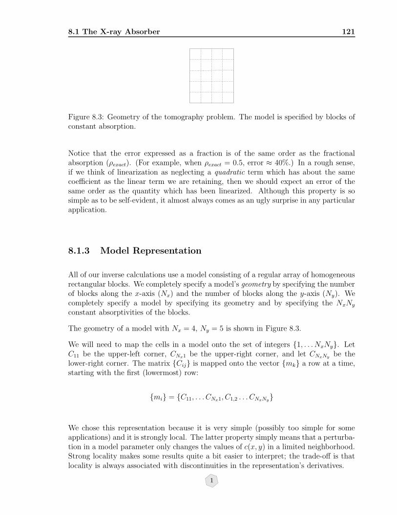
8.1 The X-ray Absorber 121
Figure 8.3: Geometry of the tomography problem. The model is specified by blocks ofconstant absorption.
Notice that the error expressed as a fraction is of the same order as the fractionalabsorption (ρexact). (For example, when ρexact = 0.5, error ≈ 40%.) In a rough sense,if we think of linearization as neglecting a quadratic term which has about the samecoefficient as the linear term we are retaining, then we should expect an error of thesame order as the quantity which has been linearized. Although this property is sosimple as to be self-evident, it almost always comes as an ugly surprise in any particularapplication.
8.1.3 Model Representation
All of our inverse calculations use a model consisting of a regular array of homogeneousrectangular blocks. We completely specify a model’s geometry by specifying the numberof blocks along the x-axis (Nx) and the number of blocks along the y-axis (Ny). Wecompletely specify a model by specifying its geometry and by specifying the NxNy
constant absorptivities of the blocks.
The geometry of a model with Nx = 4, Ny = 5 is shown in Figure 8.3.
We will need to map the cells in a model onto the set of integers 1, . . . NxNy. LetC11 be the upper-left corner, CNx1 be the upper-right corner, and let CNxNy be thelower-right corner. The matrix Cij is mapped onto the vector mk a row at a time,starting with the first (lowermost) row:
mi = C11, . . . CNx1, C1,2 . . . CNxNy
We chose this representation because it is very simple (possibly too simple for someapplications) and it is strongly local. The latter property simply means that a perturba-tion in a model parameter only changes the values of c(x, y) in a limited neighborhood.Strong locality makes some results quite a bit easier to interpret; the trade-off is thatlocality is always associated with discontinuities in the representation’s derivatives.
1
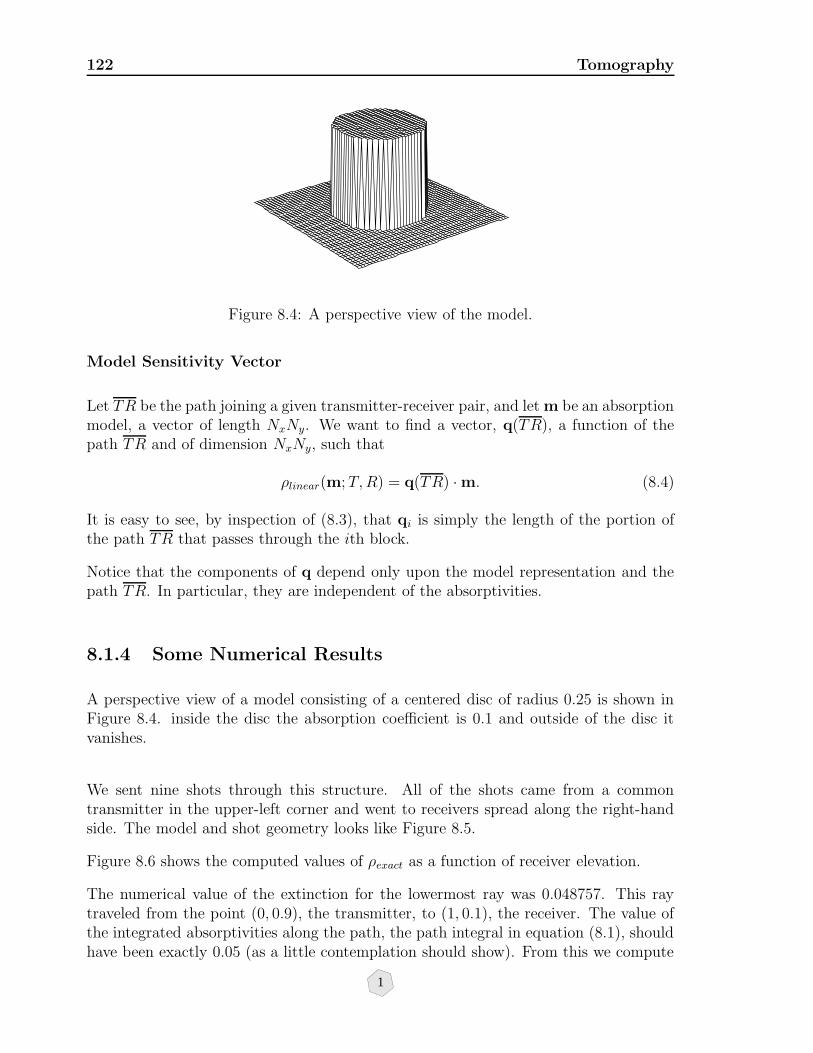
122 Tomography
Figure 8.4: A perspective view of the model.
Model Sensitivity Vector
Let TR be the path joining a given transmitter-receiver pair, and let m be an absorptionmodel, a vector of length NxNy. We want to find a vector, q(TR), a function of thepath TR and of dimension NxNy, such that
ρlinear(m;T,R) = q(TR) ·m. (8.4)
It is easy to see, by inspection of (8.3), that qi is simply the length of the portion ofthe path TR that passes through the ith block.
Notice that the components of q depend only upon the model representation and thepath TR. In particular, they are independent of the absorptivities.
8.1.4 Some Numerical Results
A perspective view of a model consisting of a centered disc of radius 0.25 is shown inFigure 8.4. inside the disc the absorption coefficient is 0.1 and outside of the disc itvanishes.
We sent nine shots through this structure. All of the shots came from a commontransmitter in the upper-left corner and went to receivers spread along the right-handside. The model and shot geometry looks like Figure 8.5.
Figure 8.6 shows the computed values of ρexact as a function of receiver elevation.
The numerical value of the extinction for the lowermost ray was 0.048757. This raytraveled from the point (0, 0.9), the transmitter, to (1, 0.1), the receiver. The value ofthe integrated absorptivities along the path, the path integral in equation (8.1), shouldhave been exactly 0.05 (as a little contemplation should show). From this we compute
1

8.1 The X-ray Absorber 123
•
•
Figure 8.5: The model and shot geometry.
• ••
•
•
•
• • •
Receiver0.2 0.4 0.6 0.8
0.0
0.01
0.02
0.03
0.04
0.05
Figure 8.6:
1

124 Tomography
r
r
r
r
r
s
Figure 8.7: Plan view of the model showing one source and five receivers.
ρtrue = 0.048771, which is in satisfactory agreement. (Note that the linearized estimateis exactly 0.05 and it is about 1% high.)
8.2 Travel Time Tomography
Along the same lines as the x-ray absorption problem, the time-of-flight of a wavepropagating through a medium with wavespeed v(x, y, z) is given by the line integralalong the ray of the reciprocal wavespeed (slowness or index of refraction)
∫
v(x,y,z)
dλ
v(x, y, z).
The problem is to infer the unknown wavespeed of the medium from repeated obser-vations of the time-of-flight for various transmitter/detector locations. For the sakeof definiteness, let’s suppose that the source emits pressure pulses, the receiver is ahydrophone, and the medium is a fluid.
Figure (8.7) shows a 2D model of an anomaly embedded in a homogeneous medium.Also shown are 5 hypothetical rays between a source and 5 detectors. This is an idealizedview on two counts. The first is that not only is the raypath unknown–rays refract–butthe raypath depends on the unknown wavespeed. This is what makes the travel timeinversion problem nonlinear. On the other hand, if we can neglect the refraction of theray, then the problem of determining the wavespeed from travel time observations iscompletely linear.
1
8.3 Computer Example: Cross-well tomography 125
The second complicating factor is that a “travel time” is only unambiguously defined atasymptotically high frequencies. In general, we could define the travel time in variousways: first recorded energy above a threshold, first peak after the threshold value issurpassed, and others. Further, the travel times themselves must be inferred from therecorded data, although it is possible in some cases that this can be done automatically;perhaps by using a triggering mechanism which records a time whenever some thresholdof activity is crossed.
For purposes of this example, we will neglect both of these difficulties. We will computethe travel times as if we were dealing with an infinite frequency (perfectly localized)pulse, and we will assume straight ray propagation. The first assumption is made inmost travel time inversion calculations since there is no easy way around the difficultywithout invoking a more elaborate theory of wave propagation. The second assumption,that of linearity, is easily avoided in practice by numerically tracing rays through theapproximate medium. But we won’t worry about this now.
8.3 Computer Example: Cross-well tomography
In the code directory you will find various implementations of straight-ray tomography.These are extensive codes and will not be described in detail here. They begin bysetting up the source/receiver geometry of the problem, computing a Jacobian matrixand fake travel times, adding noise to these and doing the least squares problem viaSVD. Here we just show some of the results that you will be able to get.
In Figure (8.8) you see a plot of the Jacobian matrix itself. The i − j element of thismatrix is the length the i-th ray travels in the j-th cell. This comes from discretizingthe travel time integral (t =
∫s(r)d`) along each ray (one for each travel time). Black
indicates zero elements and white nonzero. This particular matrix is about 95% sparse,so until we take advantage of this fact, we’ll be doing a lot of redundant operations,e.g., 0× 0 = 0.
Below this we show the “hit count”. This is the summation of the ray segments withineach cell of the model and represents the total “illumination” of each cell.
Below this we show the exact model whose features we will attempt to reconstruct viaa linear inversion.
Finally, before we can do an inversion, we need some data to invert. First we’ll computethe travel times in the true model shown above, then we’ll compute the travel timesthrough a background model which is presumed to be correct except for the absence ofthe anomaly. It’s the difference between these two that we take to be the right handside of the linear system
Jδm = δd
relating model perturbations to data perturbations. The computed solutions are shown
1
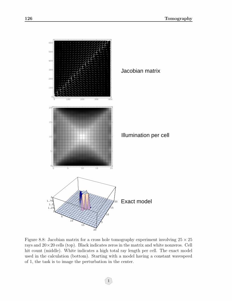
126 Tomography
0 100 200 300 4000
100
200
300
400
500
600
0 5 10 15 200
5
10
15
20
5
10
15
20
5
10
15
20
1
1.25
1.5
1.75
2
5
10
15
20
5
10
15
20
1
1.25
1.5
1.75
2
Jacobian matrix
Illumination per cell
Exact model
Figure 8.8: Jacobian matrix for a cross hole tomography experiment involving 25× 25rays and 20×20 cells (top). Black indicates zeros in the matrix and white nonzeros. Cellhit count (middle). White indicates a high total ray length per cell. The exact modelused in the calculation (bottom). Starting with a model having a constant wavespeedof 1, the task is to image the perturbation in the center.
1

8.3 Computer Example: Cross-well tomography 127
in Figure 8.9.
Finally, in Figure (8.10), we show the spectrum of singular values present in the jacobianmatrix, and one well resolved and one poorly resolved model singular vectors. Notewell that in the cross hole situation, vertically stratified features are well resolved whilehorizontally stratified features are poorly resolved. Imagine the limiting case of purelyhorizontal rays. A v(z) model would be perfectly well resolved, but a v(x) model wouldbe completely ambiguous.
1

128 Tomography
5
10
15
20
5
10
15
20
0.91
1.11.21.3
5
10
15
20
5
10
15
20
0.91
1.11.21.3
5
10
15
20
5
10
15
20
1
1.2
1.4
5
10
15
20
5
10
15
20
1
1.2
1.4
5
10
15
20
5
10
15
20
11.251.5
1.75
2
5
10
15
20
5
10
15
20
11.251.5
1.75
2
SVD reconstructions
First 10 singular values
First 50 singular values
All singular values above tolerance
Figure 8.9: SVD reconstructed solutions. Using the first 10 singular values (top).Using the first 50 (middle). Using all the singular values above the machine precision(bottom).
1
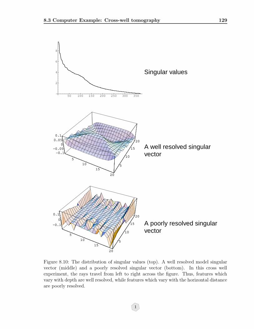
8.3 Computer Example: Cross-well tomography 129
50 100 150 200 250 300 350
2
4
6
8
5
10
15
20
5
10
15
20
-0.1-0.05
00.050.1
5
10
15
20
5
10
15
20
-0.1-0.05
00.050.1
5
10
15
20
5
10
15
20
-0.1
0
0.1
5
10
15
20
5
10
15
20
-0.1
0
0.1
Singular values
A well resolved singular vector
A poorly resolved singular vector
Figure 8.10: The distribution of singular values (top). A well resolved model singularvector (middle) and a poorly resolved singular vector (bottom). In this cross wellexperiment, the rays travel from left to right across the figure. Thus, features whichvary with depth are well resolved, while features which vary with the horizontal distanceare poorly resolved.
1

130 Tomography
1

Chapter 9
From Bayes to Weighted LeastSquares
In the last chapters we have developed the theory of least squares estimators for linearinverse problems in which the only uncertainty was the random errors in the data. Nowwe return to our earlier discussion of Bayes theorem and show how within the Bayesianstrategy we can incorporate prior information on model parameters and still get awaywith solving weighted least squares calculations.
Denote by f(m,d) the joint distribution on models and data. Recall that from Bayes’theorem, the conditional probability on m given d is
p(m|d) =f(d|m)ρ(m)
h(d),
where f(d|m) measures how well a model fits the data, ρ(m) is the prior model distri-bution, and h(d) is the marginal density of d. The conditional probability p(m|d) isthe so-called Bayesian posterior probability, expressing the idea that p(m|d) assimilatesthe data and prior information.
For now we will assume that all uncertainties (model and data) can be described byGaussian distributions. Since any Gaussian distribution can be characterized by itsmean and covariance, this means that we must specify a mean and covariance for boththe a priori distribution and the data uncertainties.
In this case the Bayesian posterior probability is the normalized product of the followingtwo functions:
√(2π)−n
detCDexp
[−1
2(g(m)− dobs)TC−1
D (g(m)− dobs)],
(9.1)
where dobs is the vector of observed data which dimension is n, CD is the data covari-
1

132 From Bayes to Weighted Least Squares
ance matrix and g(m) is the forward operator; and
√(2π)−m
detCMexp
[−1
2(m−mprior)TC−1
M (m−mprior)],
(9.2)
where m is the number of model parameters and CM is the covariance matrix describingthe distribution of models about the prior model mprior. If the forward operator islinear, then the posterior distribution is itself a Gaussian. If the forward operator isnonlinear, then the posterior is non-Gaussian.
The physical interpretation of Equation 9.1 is that it represents the probability that agiven model predicts the data. Remember that
d = g(mtrue) + e
where e is the noise. If we take expectations of both sides then
E[d] = g(mtrue) + E[e].
So if the errors are zero mean then the true model predicts the mean of the data. Ofcourse, we don’t know the true model, but if we have an estimate of it, say m theng(m) is an estimate of the mean of the data and d− g(m) is an estimate of e.
If we want to estimate the true model we still have the problem of defining what sortof estimator we want to use. Maybe this is not what we want. It may suffice to findregions in model space which have a high probability, as measured by the posterior.But for now let’s consider the problem of estimating the true model. A reasonablechoice turns out to be: look for the mean of the posterior.a If the forward operator islinear (so that g(m) = Gm for some matrix G), then Tarantola [Tar87] shows that thenormalized product
σ(m) ∝ exp−1
2
[(Gm− dobs)
TC−1D (Gm− dobs)
+ (m−mprior)TC−1
M (m−mprior)]. (9.3)
can be written as
σ(m) ∝ exp[(m−mmap)TC−1
M ′(m−mmap)], (9.4)
where
CM ′ =[GTC−1
D G+ C−1M
]−1, (9.5)
is the covariance matrix of the posterior probability. This is approximately true evenwhen g is nonlinear, provided it’s not too nonlinear.
aWe will take up the reasonableness of this choice later.
1

BIBLIOGRAPHY 133
Here mmap is the maximum of the posterior distribution, which for a Gaussian is alsothe mean. So to find our estimator we need to optimize Equation 9.3. But that isequivalent to minimizing the exponent:
minm
[(Gm− dobs)
TC−1D (Gm− dobs) + (m−mprior)
TC−1M (m−mprior)
]. (9.6)
But this is nothing but a weighted least squares problem. This is even easier to see ifwe introduce the square roots of the covariance matrices. Then the first term above is
((C−1/2D )T (Gm− dobs), C
−1/2D (Gm− dobs)
)= ‖C−1/2
D (Gm− dobs)‖2
while the second term is‖C−1/2
M (m−mprior)‖2.
Here we have used two important facts. This first is that the inverse of a symmetricmatrix is symmetric. The second is that every symmetric matrix has a square root. Tosee this consider the diagonalization of such a matrix via an orthogonal transformation:
A = QΛQT .
So it is not too hard to see that
A =(QΛ1/2QT
) (QΛ1/2QT
)= QΛ1/2Λ1/2QT = QΛQT
where the meaning of Λ1/2 is clear since it is diagonal with real elements. So QΛ1/2QT
is the square root of A.
Bibliography
[Tar87] A. Tarantola. Inverse Problem Theory. Elsevier, New York, 1987.
1

134 BIBLIOGRAPHY
1
Chapter 10
Bayesian versus FrequentistMethods of Inference
If we are Bayesians, then all prior information about models must be cast in the formof probabilities. However, in some cases, prior information is purely deterministic. Forexample, we know based on definition, that mass density and wavespeed are positive.There is nothing uncertain about this information. On the other hand, we know fromobservation that the average mass density of the Earth is less than 7g/cm2. In priciplewe can convert these pieces of deterministic information into probabilities. In thischapter we will compare and contrast the Bayesian and frequentist views of inference.This chapter is adapted from [SS97b] and [ST01].
There are two fundamentally different meanings of the term ‘probability’ in commonusage [SS97a]. If we toss a coin N times, where N is large, and see roughly N/2heads, then we say the probability of getting a head in a given toss is about 50%. Thisinterpretation of probability, based on the frequency of outcomes of random trails, istherefore called ‘frequentist’. On the other hand it is common to hear statements suchas: ‘the probability of rain tomorrow is 50%’. Since this statement does not refer to therepeated outcome of a random trial, it is not a frequentist use of the term probability.Rather, it conveys a statement of information (or lack thereof). This is the Bayesian useof ‘probability’. Both ideas seem natural to some degree, so it is perhaps unfortunatethat the same term is used to describe them.
Bayesian inversion has gained considerable popularity in its application to geophysicalinverse problems. The philosophy of this procedure is as follows. Suppose one knowssomething about a model before observing the data. This knowledge is cast in a prob-abilistic form and is called the prior probability model (prior means before the datahave been observed.) Bayesian inversion then provides a framework for combining theprobabilistic prior information with the information contained in the observed data inorder to update the prior information. The updated distribution is the posterior con-ditional model distribution given the data; it is what we know about the model after
1

136 Bayesian versus Frequentist Methods of Inference
we have assimilated the data and the prior information. The point of using the datais that the posterior information hopefully constrains the model more tightly than theprior model distribution.
However, the selection of a prior statistical model can in practice be somewhat shaky.For example, in a seismic survey we may have a fairly accurate idea of the realisticranges of seismic velocity and density, and perhaps even of the vertical correlationlength (if bore-hole measurements are available). However, the horizontal length scaleof the velocity and density variation is to a large extent unknown. Given this, how canBayesian inversion be so popular when our prior knowledge is often so poor? The reasonfor this is that in practice the prior model is used to regularize the posterior solution.Via a succession of different calculations, the characteristics of the prior model are oftentuned in such a way that the retrieved model has subjectively agreeable features. Butlogically, the prior distribution must be fixed before hand. The features used to tunethe prior should in fact be included as part of the prior information [GS97]. So, thepractice of using the data to tune the prior suggests that the reason for the popularityof Bayesian inversion within the Earth sciences is inconsistent with the underlyingphilosophy. A common attitude seems to be: ‘If I hadn’t believed it, I wouldn’t haveseen it.’
Since Bayesian statistics relies completely on the specification of a prior statisticalmodel, the flexibility taken in using the prior model as a knob to tune properties ofthe retrieved model is completely at odds with the philosophy of Bayesian inversion.One can, however, use an empirical Bayes approach to use data to help determine aprior distribution. But having used the data to select a prior, one has to correct theuncertainty estimates so as not to be overconfident [see Carlin and Louis [CL96]]. Thiscorrection is not usually done in geophysical Bayesian inversion.
10.0.1 Bayesian Inversion in Practice
There are two important questions that have to be addressed in any Bayesian inversion:
• How do we represent the prior information? This applies both to the prior modelinformation and to the description of the data statistics.
• How do we summarize the posterior information?
The second question is the easiest one to answer, at least in principle. It is just a matterof applying Bayes’ theorem to compute the posterior distribution. We then use thisdistribution to study the statistics of different parameter estimates. For example, we canfind credible regions for the model parameters given the data, or simply use posteriormeans as estimates and posterior standard deviations as ‘error bars’. However, veryseldom will we be able to compute all the posterior estimates analytically; we often
1

137
have to use computer-intensive approximations based on Markov Chain Monte Carlomethods [see for example, Tanner [Tan93]]. But still, a complete Bayesian analysis maybe computationally intractable.
The first question is a lot more difficult to answer. A first strategy is a subjectiveBayesian one: prior probabilities are designed to represent states of mind, prejudicesor prior experience. But, depending on the amount and type of prior information, thechoice of prior may or may not be clear. For example, if an unknown parameter, µ, mustlie between a and b, is it justified to assume that µ has a uniform prior distributionon the interval [a, b]? We will address this question in an example below, but fornow simply observe that there are infinitely many probability distributions consistentwith µ being in the interval [a, b]. To pick one may be an over-specification of theavailable information. Even an apparently conservative approach, such as taking theprobability distribution that maximizes the entropy subject to the constraint that µlies in the interval, may lead to pathologies in high-dimensional problems. This showshow difficult it may be to unambiguously select a prior statistical model. One way outof this dilemma is to sacrifice objectivity and presume that ‘probability lies in the eyeof the beholder’. Of course, this means that our posterior probability will be differentfrom yours.
A second approach attempts to make a somewhat more objective choice of priors by re-lying on theoretical considerations such as maximum entropy a [Jay82] , transformationinvariance [Tar87], or by somehow using observations to estimate a prior. This latterapproach is the empirical Bayes mentioned in a previous section. For example, supposeone is doing a gravity inversion to estimate mass density in some reservoir. Supposefurther that there are available a large number of independent, identically distributedlaboratory measurements of density for rocks taken from this reservoir (a big if!). Thenone could use the measurements to estimate a probability distribution for mass densitythat could be used as a prior for the gravity inversion. This is the approach taken in[GS98], where in-situ (bore-hole) measurements are used to derive an empirical priorfor surface seismic data.
An empirical Bayes analysis is basically an approximation to a full hierarchical Bayesanalysis based on the joint probability distribution of all parameters and available data.In other words, in a full Bayesian analysis the prior distribution may depend on someparamaters which in turn follow a second-stage prior. This latter prior can also dependon some third-stage prior, etc. This hierachical model ends when all the remainingparameters are assumed known. We can use the empirical Bayes approach when thelast parameters can not be assumed to be known. Instead, we use the data to estimatethe remaining parameters and stop the sequence of priors. We then proceed as in thestandard Bayesian procedure. For an introduction to empirical and hierarchical Bayesmethods see Casella [Cas85], Gelman et al. [GCSR97] and references therein. For areview on the development of objective priors see Kass and Wasserman [KW96].
aSee the appendix on entropy.
1

138 Bayesian versus Frequentist Methods of Inference
A third strategy is to abandon Bayes altogether and use only deterministic prior infor-mation about models: wave-speed is positive (a matter of definition); velocity is lessthan the speed of light (a theoretical prediction); the Earth’s average mass density isless than 7 g/cm3 (a combination of observation and theory that is highly certain).The inference problem is still statistical since random data uncertainties are taken intoaccount. Essentially the idea is to look at the set of all models that fit the data. Thenperform surgery on this set, cutting away those models that violate the deterministiccriteria, e.g., have negative density. The result will be a (presumably smaller and morerealistic) set of models that fit the data and satisfy the prior considerations. We chooseany model that fits the data to a desired level and satisfies the prior model constraints.Tikhonov’s regularization is one way of obtaining an inversion algorithm by restrictingthe family of models that fit the data; for example, among all the models that fit thedata, we choose one that has particular features, the smoothest, the shortest, etc.
10.0.2 Bayes vs Frequentist
In the Bayesian approach, probability distributions are the fundamental tools. Bayesianscan speak of the probability of a hypothesis given some evidence, and are able to conductpre-data and post-data inferences. Frequentists, on the other hand, are more concernedwith pre-data inference and run into difficulties when trying to give post-data interpre-tations to their pre-data formulation. In other words, uncertainty estimates, such asconfidence sets, are based on the error distribution, which is assumed to be known apriori, and on hypothetical repetitions of the data gathering process.
We have seen that the choice of prior distributions is not always well defined. In thiscase it would seem more reasonable to follow a frequentist approach. But it may also bethe case that the determinism that frequentists rely on in the definition of parametersmay be ill-defined. For instance, if we are trying to estimate the mass of the earth, isthis a precisly defined, non-random quantity? Perhaps, but does the definition includethe atmosphere? If so, how much of the atmosphere? If not, does it take into accountthat the mass is constantly changing (slightly) from, for example, micrometeorites?Even if you make the ‘true mass of the Earth’ well-defined (it will still be arbitrary tosome extent), it can never be precisely known.
So, which approach is better? Bayesians are happy to point to some well known in-consistencies in the frequentist methodology and to difficulties frequentists face to useavailable prior information. Some Bayesians even go as far as claiming that anyone inher/his right frame of mind should be a Bayesian. Frequentists, on the other hand,complain about the sometimes subjective choice of priors and about the computationalcomplexity of the Bayesian approach. In real down-to-earth data analysis we prefer tokeep an open mind. Different methods may be better than others depending on theproblem. Both schools of inference have something to offer. For colorful discussions onthe comparison of the two approaches see Efron [Efr86] and Lindley [Lin75].
1

10.1 What Difference Does the Prior Make? 139
10.1 What Difference Does the Prior Make?
In a Bayesian calculation, whatever estimator we use depends on the prior and condi-tional distributions given the data. There is no clear established procedure to checkhow much information a prior injects into the posterior estimates. [This is one of theopen problems mentioned in Kass and Wasserman [KW96].] In this example we willcompare the risks of the estimators.
To measure the performance of an estimator, m, of m we define the loss function,L(m, m); L is a non-negative function which is zero for the true model. That is, forany other model m1, L(m,m1) ≥ 0 and L(m,m) ≡ 0. The loss is a measure of the costof estimating the true model with m when it is actually m. For example, a commonloss function is the square error: L(m, m) = (m − m)2. But there are other choiceslike `p-norm error: L(m, m) = ‖m− m‖p.
The loss, L(m, m), is a random variable since m depends on the data. We average overthe data to obtain an average loss. This is called the risk of m given the model m
R(m, m) = EP L(m, m), (10.1)
where P is the error probability distribution and EP the expectation with respect tothis distribution. For square error loss the risk is the usual mean square error.
10.1.1 Bayes Risk
The expected loss depends on the chosen model. Some estimators may have small risksfor some models but not for others. To compare estimators we need a global measurethat takes all plausible models into account. A natural choice is to take the expectedvalue of the loss with respect to the posterior distribution, p(m|d), of the model giventhe data. This is called the posterior risk
rm|d = Em|d L[m, m(d)].
Alternatively we can take a weighted average of the risk (10.1) using the prior modeldistribution as weight function. This is the Bayes risk
rρ = Eρ R(m, m),
where ρ is the prior model distribution. An estimator with the smallest Bayes risk iscalled a Bayes estimator. Note that we have used a frequentist approach to definethe Bayes risk, since we have not conditioned on the observed data. It does makesense, however, to expect good frequentist behavior if the Bayesian approach is to beused repeatedly with different data sets. In addition, it can be shown that, under verygeneral conditions, minimizing the Bayes risk is equivalent to minimizing the posteriorrisk [Ber85].
1

140 Bayesian versus Frequentist Methods of Inference
Let f denote the joint distribution of models and data. The distribution (marginal) ofthe data is obtained by integrating f over the models
h(d) =∫
Mf(m,d)dm,
where M is the space of models. From Bayes’ theorem, the conditional distribution ofm given d is
p(m|d) =f(d|m)ρ(m)
h(d),
where ρ(m), the prior distribution, is the marginal of f with respect to m. The con-ditional distribution, p(m|d), is the so-called Bayesian posterior distribution, whichupdates the prior information in view of the data.
One can define a number of reasonable estimators of m based on p(m|d). For example,the m that maximizes p(m|d) (or that is close, in probability, to m.) Or one couldcompute the estimator that gives the smallest Bayes risk for a given prior and lossfunction. It can be shown [Lehmann [Leh83], p.239] that, for square error loss function,the Bayes estimator is the posterior mean.
Here is a simple example of using a normal prior to estimate a normal mean. Assumethat there are n observations, (d1, d2, ..., dn) = d, which are iid N(η, σ2) and that wewant to estimate the mean, η, given that the prior, ρ, is N(µ, β2). Up to a constantfactor, the joint distribution of η and d is [Lehmann [Leh83], p.243]
f(d, η) = exp
[− 1
2σ
n∑
i=1
(di − η)2
]exp
[− 1
2β(η − µ)2
],
The posterior mean is
η = E(η|d) =nd/σ2 + µ/β2
n/σ2 + 1/β2,
where d is the arithmetic mean of the data. The posterior variance is
Var(η|d) =1
n/σ2 + 1/β2.
Notice that the posterior variance is always reduced by the presence of a nonzero β.The posterior mean, which is the Bayes estimator for square error loss, can be writtenas
η(d) =
[n/σ2
n/σ2 + 1/β2
]d +
[1/β2
n/σ2 + 1/β2
]µ.
We see that the Bayes estimator is a weighted average of the mean of the data andthe mean of the Bayesian prior distribution; the latter is the Bayes estimator beforeany data have been observed. The Bayes risk is the integral, over the data, of theposterior variance of η. Since the posterior variance does not depend of d, the Bayesrisk is just the posterior variance. Note also that as β → 0, increasingly strong priorinformation, the estimate converges to the prior mean. As β → ∞, increasingly weakprior information, the Bayes estimate converges to the mean of the data. Also notethat as β →∞ the prior becomes improper (not normalizable).
1
10.2 Example: A Toy Inverse Problem 141
10.1.2 What is the Most Conservative Prior?
It often happens that there is not enough information to choose a prior density for theunknown parameters, or that the information available is not easily translated into aprobabilistic statement; yet we need a prior to be able to apply Bayes’ theorem. Inthis case we try to find a ‘noninformative’, or ‘conservative’, prior that will allow usto conduct the Bayesian inference while injecting a minimum of artificial information;that is, information which is not justified by the physical process.
We have defined the Bayes risk, rρ, and the Bayes estimator for a given prior density.It stands to reason that the more informative the prior the smaller its associated risk;we therefore say that a prior, ρ, is least favorable if rρ ≥ rρ′ for any other prior, ρ′. Aleast favorable prior is associated with the greatest unavoidable loss.
In the frequentist approach the greatest unavoidable loss is associated with the maxi-mum of the risk (10.1) over all the possible models. An estimator that minimizes thismaximum risk is called a minimax estimator. Under certain conditions the Bayes es-timator corresponding to a least favorable prior actually minimizes the maximum risk[see Lehmann [Leh83]]. This is true, for example, when the Bayes estimator has a con-stant risk. In this sense we can think of a least favorable prior as being a route to themost conservative Bayesian estimator.
How does one find a conservative (noninformative) prior? There is no easy answer, eventhe terms ‘conservative’ and ‘noninformative’ are not well defined. One possibility isto define a measure of information (e.g., entropy) and determine a prior which mini-mizes/maximizes this measure (e.g., maximum entropy). We could also look for priorswhich are invariant under some family of transformations.
10.2 Example: A Toy Inverse Problem
We consider a simple example of estimating the mean, η, of a unit variance normaldistribution, N(η, 1), with an observation, d, from N(η, 1) given that |η| is known tobe bounded by β. Following Stark [Sta97], we will use this as a model of an inverseproblem with a prior constraint. Without the prior bound, d is an estimator of η butwe hope to do better (obtain a smaller risk) by including the bound information. Howcan we include this information in the estimation procedure? One possibility is to usea Bayesian approach and assign a prior distribution to η which is uniform on [−β, β].We will show that this distribution injects stronger information than might be evident.
1
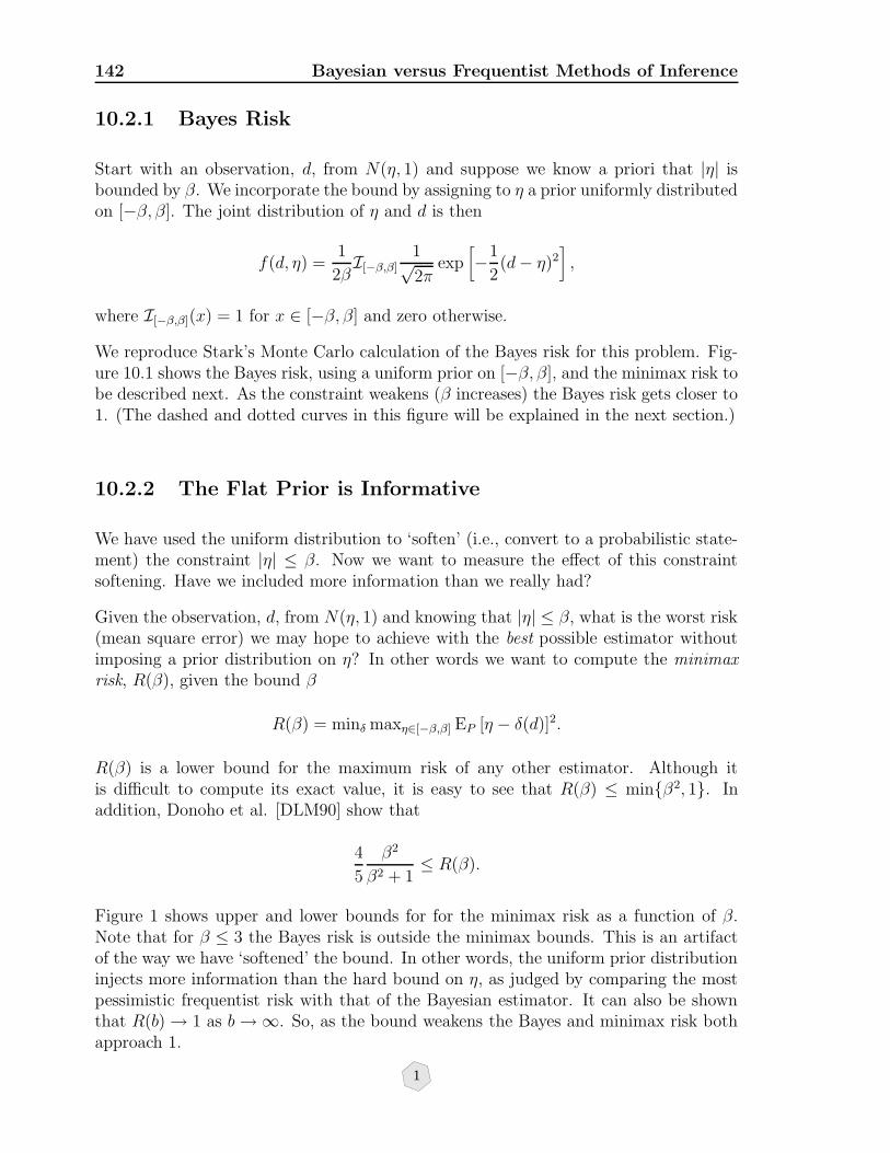
142 Bayesian versus Frequentist Methods of Inference
10.2.1 Bayes Risk
Start with an observation, d, from N(η, 1) and suppose we know a priori that |η| isbounded by β. We incorporate the bound by assigning to η a prior uniformly distributedon [−β, β]. The joint distribution of η and d is then
f(d, η) =1
2βI[−β,β]
1√2π
exp[−1
2(d− η)2
],
where I[−β,β](x) = 1 for x ∈ [−β, β] and zero otherwise.
We reproduce Stark’s Monte Carlo calculation of the Bayes risk for this problem. Fig-ure 10.1 shows the Bayes risk, using a uniform prior on [−β, β], and the minimax risk tobe described next. As the constraint weakens (β increases) the Bayes risk gets closer to1. (The dashed and dotted curves in this figure will be explained in the next section.)
10.2.2 The Flat Prior is Informative
We have used the uniform distribution to ‘soften’ (i.e., convert to a probabilistic state-ment) the constraint |η| ≤ β. Now we want to measure the effect of this constraintsoftening. Have we included more information than we really had?
Given the observation, d, from N(η, 1) and knowing that |η| ≤ β, what is the worst risk(mean square error) we may hope to achieve with the best possible estimator withoutimposing a prior distribution on η? In other words we want to compute the minimaxrisk, R(β), given the bound β
R(β) = minδ maxη∈[−β,β] EP [η − δ(d)]2.
R(β) is a lower bound for the maximum risk of any other estimator. Although itis difficult to compute its exact value, it is easy to see that R(β) ≤ minβ2, 1. Inaddition, Donoho et al. [DLM90] show that
4
5
β2
β2 + 1≤ R(β).
Figure 1 shows upper and lower bounds for for the minimax risk as a function of β.Note that for β ≤ 3 the Bayes risk is outside the minimax bounds. This is an artifactof the way we have ‘softened’ the bound. In other words, the uniform prior distributioninjects more information than the hard bound on η, as judged by comparing the mostpessimistic frequentist risk with that of the Bayesian estimator. It can also be shownthat R(b)→ 1 as b→∞. So, as the bound weakens the Bayes and minimax risk bothapproach 1.
1
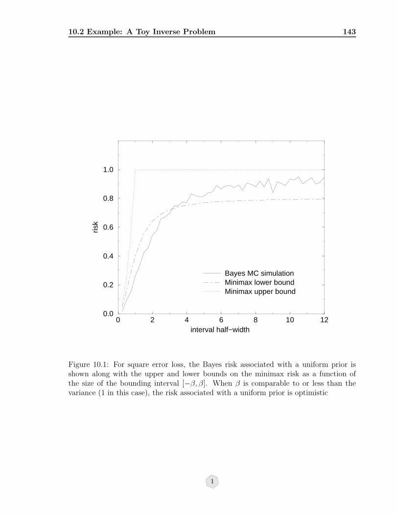
10.2 Example: A Toy Inverse Problem 143
0 2 4 6 8 10 12interval half−width
0.0
0.2
0.4
0.6
0.8
1.0
risk
Bayes MC simulationMinimax lower boundMinimax upper bound
Figure 10.1: For square error loss, the Bayes risk associated with a uniform prior isshown along with the upper and lower bounds on the minimax risk as a function ofthe size of the bounding interval [−β, β]. When β is comparable to or less than thevariance (1 in this case), the risk associated with a uniform prior is optimistic
1
144 Bayesian versus Frequentist Methods of Inference
10.3 Priors in High Dimensional Spaces: The Curse
of Dimensionality
As we have just seen, most probability distributions usually have more informationthan implied by a hard constraint. To say, for instance, that any model with ‖m‖ ≤ 1is feasible is certainly not the same thing as saying that all models with ‖m‖ ≤ 1 areequally likely. And while we could look for the most conservative or least favorablesuch probabilistic assignment, Backus [Bac88] makes an interesting argument againstany such probabilistic replacement in high- or infinite-dimensional model spaces. Hispoint can be illustrated with a simple example. Suppose that all we know about an n-dimensional model vector, m, is that its length, m ≡ ‖m‖, is less than some particularvalue–unity for the sake of definiteness. In other words, suppose we know a priorithat m is constrained to be within the n-dimensional unit ball, Bn. Backus considersvarious probabilistic replacements of this hard constraint; this is called ‘softening’ theconstraint. We could for example choose a prior probability on m which is uniform onBn. Namely, the probability that m will lie in some small volume, δV ∈ Bn, shall beequal to δV divided by the volume of Bn. Choosing this uniform prior on the ball, it isnot difficult to show that the expectation of m2 for an n-dimensional m is
E(m2) =n
n + 2
which converges to 1 as n increases. Unfortunately, the variance of m2 goes as 1/nfor large n, and thus we seem to have introduced a piece of information that was notimplied by the original constraint; namely that for large n, the only likely vectors, m,will have length equal to one. The reason for this apparently strange behavior has todo with the way volumes behave in high dimensional spaces. The volume, Vn(R), ofthe R− diameter ball in n dimensional space is
Vn(R) = CnRn,
where Cn is a constant that depends only on the dimension n, not on the radius. [Thisis a standard result in statistical mechanics; e.g., Becker [Bec67].] If we compute thevolume, Vε,n, of an n-dimensional shell of thickness ε just inside an R-diameter ball wecan see that
Vε,n ≡ Vn(R)− Vn(R− ε) = Cn(Rn − (R− ε)n)
= Vn(R)(
1−(
1− ε
R
)n). (10.2)
Now, for ε/R 1 and n 1 we have
Vε,n ≈ Vn(R)(1− e−nε/R
).
This says that as n gets large, nearly all of the volume of the ball is compressed into athin shell just inside the radius.
1
10.3 Priors in High Dimensional Spaces: The Curse of Dimensionality 145
But even this objection can be overcome with a different choice of probability distri-bution to soften the constraint. For example, choose m to be uniformly distributed on[0, 1] and choose the n−1 spherical polar angles uniformly on their respective domains.This probability is uniform on ‖m‖, but non-uniform on the ball. However it is con-sistent with the constraint and has the property that the mean and variance of m2 isindependent of the dimension of the space.
So, as Backus has said, we must be very careful in replacing a hard constraint witha probability distribution, especially in a high-dimensional model space. Apparentlyinnocent choices may lead to unexpected behavior.
Appendix: Entropy
This appendix is a brief introduction to entropy as it relates to inversion. For moredetails see [GMS01]. In Bayesian inversion we use probabilities to represent states ofinformation. But just how does one quantify such a state? Is it possible to say thatone probability has more information than another?
Consider an experiment with N possible outcomes each occuring with a probability pi.In analogy with the statistical mechanical definition of entropy, [Sha48] introduced thefollowing definition of the entropy for such discrete probabilities:
H(p) = −∑
i
pi log pi. (10.3)
Following Shannon, three postulates should be satisfied by H(p) or any other measureof information. Those are:
1. Continuity;
2. Monotonicity, and
3. Composition Law.
These postulates are discussed in detail in [GMS01], here a qualitative understanding issufficient. The first postulate requires that we should not gain or loose a large amountof information by making a small change to the probabilities. The second postulate,monotonicity, refers to the information associated with a collection of independent,equally likely events. It is clear that in such a case the uncertainty must increasemonotonically with the number of possible outcomes. The third postulate requires thatit should not matter how one regroups the events of a given set. The entropy of the setshould stay the same.
To see the meaning of Equation 10.3, consider an experiment whose outcome is knownwith absolute certainty. Then, the corresponding probability density is a Kronecker
1
146 Bayesian versus Frequentist Methods of Inference
delta pi = δiq, where q is the certain event, and H(p) = 0 (no uncertainty). If thereare two equally likely outcomes, then H(p) = −1/2 log(1/2) − 1/2 log(1/2) = log 2.Whereas if one of the events has a probability 1/10 and one has probability 9/10 thenthe entropy is H(p) = −1/10 log(1/10) − 9/10 log(9/10) = log 10 − .9 log 9, which isabout half that in the equally likely case. For M equally likely events H(p) = logM .And in the limit that M goes to infinity, then the uncertainty must too.
The usefulness of the definition 10.3 depends on the definition of the probability p. If thep is a 1D distribution associated with the frequency of outcomes of the possible events,then p is not affected by the correlation of the points. E.g., if we sample 10 pointspseudo-randomly from a probability distribution with two equally likely outcomes 0and 1, we might see something like the following
0010110110.
As luck would have it there are 5 0’s and 5 1’s. Now sort these outcomes in increasingorder
0000011111.
There are still 5 0’s and 5 1’s but we certainly would not regard the latter experimentas representing the same degree of uncertainty as the former. Similarly, if we sample1000 points independently from a Gaussian we’ll see a nice bell-shaped curve. But thefrequencies of the binned events are independent of their order. So, once again, sortingthem into monotonic order will not change the entropy. of course, the dependence(correlation) among events is not being considered by an unidimensional probabilitydistribution. Once multidimensional probabilities are used in definition (10.3), suchcorrelation can be accounted for in entropy calculations.
Now, in inverse theory we are always comparing one state of information to another—what we know before relative to what we know after. So it is more appropriate tomeasure the relative information of one probability compared to another. Let us there-fore revise the original definition of discrete entropy (Equation (10.3)), and introducethe concept of relative entropy. Thus,
H[pi; qi] = −∑
i
pi logpiqi. (10.4)
Here, qi is a discrete probability characterizing a reference state of information. Theextension of Equation (10.4) to the continuous case is clean and straightforward:
H[p(x); q(x)] = −∑
i
p(xi)∆xi logp(xi)∆xiq(xi)∆xi
= −∑
i
p(xi) logp(xi)
q(xi)∆xi
= −∫ b
ap(x) log
p(x)
q(x)dx, (10.5)
as ∆xi → 0 (or n→∞)
1
10.3 Priors in High Dimensional Spaces: The Curse of Dimensionality 147
which is finite.
We will adopt Equation (10.4) as the definition of relative entropy in the discrete case,and, as commonly done, the last expression of Equation (10.6) as the definition ofrelative entropy in the continuous case. q(x), or qi, represents a state of informationagainst which we make comparisons. Finally it is worth mentioning that the negativeof the quantity H[p(x); q(x)], known as cross-entropy, was first defined by Kullback[Kul59] as the directed divergence. This quantity defines the amount of information ofthe probability density p(x) with respect to q(x). See also [SJ81].
Convinced that entropy is a suitable measure for the uncertainty of a probability dis-tribution, Jaynes [Jay57] showed that a useful tool for conservatively assigning proba-bilities was to maximize the entropy of the unknown distribution subject to constraintson its moments.
Mathematically this variational problem can be expressed by maximizing Equation (10.4)subjected to the normalization of the distribution
N∑
i=1
p(xi) = 1, (10.6)
and to other constraints given in the form of expectations
〈wk(x)〉 =N∑
i=1
wk(xi)p(xi), k = 1, ..., K. (10.7)
This is equivalent to the unconstrained problem, given by
S(p;λ, q) = −N∑
i=1
p (xi) lnp (xi)
q (xi)
−(λ0 − 1)
[N∑
i=1
p (xi)− 1
]
−K∑
k=1
λk
[N∑
i=1
wk(xi) p (xi)− µk], (10.8)
where µk are sample estimates of 〈wk(x)〉 and the λk are the Lagrange multipliersassociated with the constraints. Note that the term (λ0− 1) is just a redefinition of thezero-order Lagrange multiplier introduced for convenience. If we take the first variationof the functional S(p;λ, q) with respect to the probabilities, we get that δS(p;λ, q)equals
N∑
i=1
[∂H
∂p(xi)− (λ0 − 1)−
K∑
k=1
λkwk(xi)
]δp(xi), (10.9)
with∂H
∂p(xi)= −
[lnp (xi)
q (xi)+ 1
]. (10.10)
1
148 BIBLIOGRAPHY
The solution to the problem can be found in the usual way by letting δS(p) = 0, whichyields
p(xi) = q(xi) exp
[−λ0 −
K∑
k=1
λkwk(xi)
], (10.11)
or
p(xi) = Z−1q(xi) exp
[−
K∑
k=1
λkwk(xi)
], (10.12)
with
Z ≡ exp(λ0) =N∑
i=1
q(xi) exp
[−
K∑
k=1
λkwk(xi)
]. (10.13)
However, to determine the maximum-entropy probability function we still need to findthe values for the other Lagrange multipliers and to specify the prior probability q(xi).Techniques and examples of maximum entropy calculations of this sort are describedin [GMS01].
Bibliography
[Bac88] G. Backus. Hard and soft prior bounds in geophysical inverse problems.Geophysical Journal, 94:249–261, 1988.
[Bec67] Richard Becker. Theory of Heat. Springer-Verlag, 1967.
[Ber85] L. O. Berger. Statistical Decision Theory and Bayesian Analysis. Springer-Verlag, 1985.
[Cas85] G. Casella. An introduction to empirical Bayes data analysis. The AmericanStatistician, 39:83–87, 1985.
[CL96] B. P. Carlin and T. A. Louis. Bayes and Empirical Bayes Methods for DataAnalysis. Chapmann & Hall, 1996.
[DLM90] D. L. Donoho, R. C. Liu, and K. B. MacGibbon. Mimimax risk over hyper-rectangles, and implications. Annals of Statistics, 18:1416–1437, 1990.
[Efr86] B. Efron. Why isn’t everyone a Bayesian. American Statistician, 40(1):1–11,1986.
[GCSR97] A. Gelman, J. B. Carlin, H. S. Stern, and D. B. Rubin. Bayesian DataAnalysis. Chapman & Hall, 1997.
[GMS01] W. Gouveia, F. Moraes, and J. A. Scales. Entropy, Information and Inver-sion. 2001. http://samizdat.mines.edu.
[GS97] W. Gouveia and J. A. Scales. Resolution in seismic waveform inversion:Bayes vs occam. Inverse Problems, 13:323–349, 1997.
1

BIBLIOGRAPHY 149
[GS98] W.P. Gouveia and J.A. Scales. Bayesian seismic waveform inversion: Pa-rameter estimation and uncertainty analysis. JGR, 103:2759–2779, 1998.
[Jay57] E. T. Jaynes. Information theory and statistical mechanics. Phys. Rev.,106:171–190, 1957.
[Jay82] E. T. Jaynes. On the rationale of maximum entropy methods. Proceedingsof IEEE, 70:939–952, 1982.
[Kul59] S. Kullback. Information Theory and Statistics. Wiley, New York, N. Y.,1959. Plublished by Dover in 1968.
[KW96] R. Kass and L. Wasserman. The selection of prior distributions by formalrules. Journal of the American Statistical Association, 91:1342–1370, 1996.
[Leh83] E. Lehmann. Theory of point estimation. Wiley, 1983.
[Lin75] D. V. Lindley. The future of statistics–A Bayesian 21st century. In Proceed-ings of the Conference on Directions for Mathematical Statistics. 1975.
[Sha48] C. E. Shannon. A mathematical theory of communication. Bell SystemsTechnical Jour., 27:379–423,623–656, 1948.
[SJ81] J. E. Shore and R. W. Johnson. Properties of cross–entropy minimization.IEEE Trans. on Information Theory, IT-27:472–482, 1981.
[SS97a] J. A. Scales and R. Snieder. To Bayes or not to Bayes? Geophysics, 63:1045–1046, 1997.
[SS97b] J.A. Scales and R. Snieder. To Bayes or not to Bayes. Geophysics, 62:1045–1046, 1997.
[ST01] J.A. Scales and L. Tenorio. Prior information and uncertainty in inverseproblems. Geophyusics, 66:389–397, 2001.
[Sta97] P. B. Stark. Does God play dice with the Earth? (And if so, are theyloaded?). Talk given at the 1997 SIAM Geosciences Meeting, Albuquerque,NM, 1997. http://www.stat.Berkeley.EDU/users/stark/.
[Tan93] M. A. Tanner. Tools for Statistical Inference. Methods for the Explorationof Posterior Distributions and Likelihood Functions. Springer-Verlag, 1993.
[Tar87] A. Tarantola. Inverse Problem Theory. Elsevier, New York, 1987.
1

150 BIBLIOGRAPHY
1

Chapter 11
Iterative Linear Solvers
We have seen throughout the course that least squares problems are ubiquitous in in-verse theory for two main reasons. First, least squares gives rise to linear problems,which are relatively easy to deal with. And secondly, finding the maximum of a Gaus-sian distribution is a least squares problem. That means that if the final a posterioriprobability on the models is Gaussian, then finding the maximum a posteriori (MAP)model amounts to solving a weighted least squares problem. For both reasons, leastsquares is very important and a number of specialized numerical techniques have beendeveloped. In this chapter we digress and discuss a very useful class of iterative algo-rithms for solving linear systems. These methods are at the core of most large-scaleinverse calculations.
11.1 Classical Iterative Methods for Large Systems
of Linear Equations
A direct method for solving linear systems involves a finite sequence of steps, thenumber of which is known in advance and does not depend on the matrix involved.Usually nothing can be gained by halting a direct method early; it’s all or nothing.If the matrix is sparse, direct methods will almost always result in intermediate fill,the creation of new nonzero matrix elements during the solution. Fill can usually bemitigated by carefully ordering operations and/or the matrix elements. Even so, directmethods for sparse linear systems require a certain amount of sophistication and carefulprogramming. On the other hand, iterative methods start with some approximation,perhaps random, to the solution of the linear system and refine it successively until some“stopping criterion” is satisfied. Most iterative methods do not require the matrix tobe explicitly defined; it often suffices to know the action of the matrix (and perhaps itstranspose) on arbitrary vectors. As a result, fill does not occur and the data structuresnecessary to store and manipulate the matrix elements can be quite simple. The general
1

152 Iterative Linear Solvers
subject of iterative methods is vast and in no sense will a survey be attempted. The aimof the first section is simply to get the ball rolling and introduce a few classical methodsbefore diving into conjugate gradient. In addition, the classical iterative methods aremostly based on matrix “splitting” which plays a key role in preconditioned conjugategradient. This brief discussion is patterned on Chapter 8 of [SB80] and Chapter 4of [You71]. Young is the pioneer in computational linear algebra and his book is thestandard reference in the field.
Let A be a nonsingular n×n matrix and x = A−1h be the exact solution of the system
Ax = h. (11.1)
A general class of iterative methods is of the form
xi+1 = Φ(xi), i = 0, 1, 2, . . . (11.2)
where Φ is called the iteration function. A necessary and sufficient condition for (11.2)to converge is that the spectral radiusa of Φ be less than one. For example, taking(11.1), introduce an arbitrary nonsingular matrix B via the identity
Bx + (A−B)x = h. (11.4)
Then, by making the ansatz
Bxi+1 + (A− B)xi = h (11.5)
one has
xi+1 = xi − B−1(Axi − h) = (I −B−1A)xi +B−1h. (11.6)
In order for this to work one must be able to solve (11.5). Further, the closer B is toA, the smaller the moduli of the eigenvalues of I −B−1A will be, and the more rapidlywill (11.6) converge. Many of the common iterative methods can be illustrated withthe following splitting.
A = D − E − F (11.7)
where D = diag(A), −E is the lower triangular part of A and−F is the upper triangularpart of A. Now, using the abbreviations
L ≡ D−1E, U ≡ D−1F, J ≡ L+ U, H ≡ (I − L)−1U (11.8)
and assuming ai,i 6= 0 ∀i, one has
aThe spectral radius of an operator is the least upper bound of its spectrum σ:
ρ(Φ) ≡ supλ∈σ(Φ)
| λ | (11.3)
1

11.1 Classical Iterative Methods 153
Algorithm 1 Jacobi’s Method
B = D, I − B−1A = J (11.9)
aj,jxj(i+1) +∑
k 6=jaj,kxk(i) = hj j = 1, 2, . . . , n, i = 0, 1, . . . (11.10)
where the subscript in parentheses refers to the iteration number. Jacobi’s method isalso called the “total step method.” To get the “single step” or Gauss-Seidel methodchoose B to be the lower triangular part of A including the diagonal:
Algorithm 2 Gauss-Seidel Method
B = D − E, I − B−1A = (I − L)−1U = H (11.11)∑
k<j
aj,kxk(i+1) + aj,jxj(i+1) +∑
k>j
aj,kxk(i) = hj j = 1, 2, . . . , n, i = 0, 1, . . . (11.12)
More generally still, one may consider using a class of splitting matrices B(ω) dependingon a parameter ω, and choosing ω in such a way as to make the spectral radius ofI−B−1(ω)A as small as possible. The “relaxation” methods are based on the followingchoice for B:
Algorithm 3 Relaxation Methods
B(ω) =1
ωD(I − ωL) (11.13)
B(ω)xi+1 = (B(ω)− A)xi + h i = 0, 1, . . . (11.14)
For ω > 1 this is called overrelaxation, while for ω < 1 it is called underrelaxation.For ω = 1 (11.14) reduces to Gauss-Seidel. The rate of convergence of this method isdetermined by the spectral radius of
I −B−1(ω)A = (I − ωL)−1[(1− ω)I + ωU ] (11.15)
The books by Young [You71] and Stoer & Bulirsch [SB80] have many convergenceresults for relaxation methods. An important one, due to Ostrowski and Reich is:
Theorem 12 For positive definite matrices Ab
ρ(I −B−1(ω)A) < 1 ∀ 0 < ω < 2. (11.16)
In particular, the Gauss-Seidel method (ω = 1) converges for positive definite matrices.
For a proof of this result, see [SB80], pages 547–548. This result can be considerablysharpened for what Young calls type-A matrices or the “consistently ordered” matrices(see, for example, [You71], chapter 5).
bA matrix A is positive if (x,Ax) ≥ 0 for all x. It is positive definite if the inequality is strict.
1

154 Iterative Linear Solvers
11.2 Conjugate Gradient
Conjugate gradient is by far the most widely used iterative method for solving largelinear systems. In its simplest forms it is easy to program and use, yet retains theflexibility to tackle some very demanding problems. Theoretically, CG is a descendantof the method of steepest descent, which is where the discussion begins. But first, afew definitions.
11.2.1 Inner Products
We will assume that vectors lie in finite dimensional Cartesian spaces such as Rn. Aninner product is a scalar-valued function on Rn × Rn, whose values are denoted by(x,y), which has the following properties:
positivity (x,x) ≥ 0; (x,x) = 0⇔ x = 0 (11.17)
symmetry (x,y) = (y,x) (11.18)
linearity (x,y + z) = (x,y) + (x, z) (11.19)
continuity (αx,y) = α(x,y). (11.20)
This definition applies to general linear spaces. A specific inner product for Cartesianspaces is (x,y) ≡ xT · y =
∑ni=1 xiyi
11.2.2 Quadratic Forms
A quadratic form on Rn is defined by
f(x) =1
2(x, Ax)− (h,x) + c (11.21)
where A ∈ Rn×n; h,x ∈ Rn; and c is a constant. The quadratic form is said to besymmetric, positive, or positive definite, according to whether the matrix A has theseproperties. The gradient of a symmetric quadratic form f is
f ′(x) = Ax− h. (11.22)
This equation leads to the key observation: finding critical points of quadratic forms(i.e., vectors x where f ′(x) vanishes) is very closely related to solving linear systems.
1
11.2 Conjugate Gradient 155
11.2.3 Quadratic Minimization
The fact that solutions of Ax = h can be maxima or saddle points complicates thingsslightly. We will use the concept of positivity for a matrix. A matrix A is said to bepositive if (x, Ax) ≥ 0 for all x. So one must make a few assumptions which are clarifiedby the following lemma.
Lemma 2 Suppose that z is a solution of the system Az = h, A is positive and sym-metric, and f(x) is the quadratic form associated with A, then
f(x) = f(z) +1
2((x− z), A(x− z)). (11.23)
This means that z must be a minimum of the quadratic form since the second term onthe right is positive. Thus the value of f at an arbitrary point x must be greater thanits value at z. To prove this, let x = z + p where Az = h. Then
f(x) = f(z + p) =1
2((z + p), A(z + p))− (h, (z + p)) + c.
= f(z) +1
2(z, Ap) + (p, Az) + (p, Ap) − (h,p).
If A is symmetric, the first two terms in brackets are equal, hence:
f(x) = f(z) +1
2(p, Ap) + (Az,p)− (h,p).
But by assumption Az = h, so that
f(x) = f(z) +1
2(p, Ap) = f(z) +
1
2((x− z), A(x− z))
which completes the proof.
As a corollary one observes that if A is positive definite as well as symmetric, then z isthe unique minimum of f(z) since in that case the term ((x− z), A(x− z)) is equal tozero if and only if x = z. It will be assumed, unless otherwise stated, that the matricesare symmetric and positive definite.
The level surfaces of a positive definite quadratic form (i.e, the locus of points for whichf(x) is constant) is an ellipsoid centered about the global minimum. And the semiaxesof this ellipsoid are related to the eigenvalues of the defining matrix.
The negative gradient of any function points in the direction of steepest descent of thefunction. Calling this direction r one has
r = −f ′(x) = h− Ax = A(z− x) (11.24)
since Az = h. The idea behind the method of steepest descents is to repeatedlyminimize f along lines defined by the residual vector. A prescription for this is givenby the following lemma.
1

156 Iterative Linear Solvers
Lemma 3 For some choice of a constant α
f(x) = f(x + 2αr) (11.25)
f(x + αr)− f(x) ≤ 0 (11.26)
where r is the residual vector and x is arbitrary.
In other words, there exists a constant α such that by moving by an amount 2α alongthe residual, one ends up on the other side of the ellipsoid f(x) = constant. Andfurther, if one moves to the midpoint of this line, one is assured of being closer to (or atthe very least, not farther away from) the global minimum. The proof of this assertionis by construction. From the definition of f one has for arbitrary x, α
f(x + 2αr) =1
2((x + 2αr), A(x + 2αr))− (h, (x + 2αr)) + c
= f(x) +1
2(2αr, Ax) + (2αr, A2αr) + (x, A2αr) − (h, 2αr)
= f(x) + 2α(r, Ax) + 2α2(r, Ar)− 2α(h, r)
= f(x)− 2α(r, r) + 2α2(r, Ar)
using Ax = h− r.
Therefore, choosing α to be (r, r)/(r, Ar) implies that f(x + 2αr) = f(x). Repeatingthe argument for f(x + αr) with the same choice of α, one sees immediately that
f(x + αr) = f(x)− 1
2
(r, r)2
(r, Ar)≤ f(x)
which completes the proof for A symmetric and positive definite.
This lemma provides all that is necessary to construct a globally convergent gradi-ent algorithm for finding the solutions of symmetric, positive definite linear systems,or equivalently, finding the minima of positive definite quadratic forms. By globallyconvergent we mean that it converges for any starting value.
Algorithm 4 Method of Steepest Descent Choose x0. This gives r0 = h − Ax0.Then for k = 1, 2, 3, . . .
αk = (rk−1, rk−1)/(rk−1, Ark−1),xk = xk−1 + αkrk−1
rk = h− Axk
(11.27)
Since it has already been shown that f(x + αr) ≤ f(x) for any x, it follows that
f(x0) ≥ f(x1) ≥ . . . ≥ f(xk) . . . (11.28)
1
11.2 Conjugate Gradient 157
is a monotone sequence which is bounded below by the unique minimum f(z). Thatsuch a sequence must converge is intuitively clear and indeed follows from the MonotoneConvergence Theorem. The proof of this theorem relies on a surprisingly deep propertyof real numbers: any nonempty set of real numbers which has a lower bound, has agreatest lower bound (called the infinum). Having thus established the convergence off(xk) to f(z), the convergence of xk to z follows from Lemma 2 and the properties ofinner products:
f(z)− f(xk) = −1
2(xk − z, A(xk − z))→ 0⇒ xk − z→ 0 (11.29)
since A is positive definite.
There is a drawback to steepest descent, which occurs when the ratio of the largestto the smallest eigenvalue (the condition number κ) is very large; the following resultquantifies ill-conditioning for quadratic minimization problems.
Theorem 13 Let λmax and λmin be the largest and smallest eigenvalues of the sym-metric positive definite matrix A. Let z be the minimum of f(x) and r the residualassociated with an arbitrary x. Then
‖ r ‖2λmax
≤ f(x)− f(z) ≤ ‖ r ‖2λmin
(11.30)
where ‖ x ‖2≡ (x,x) is the Euclidean norm.
If all the eigenvalues of A were the same, then the level surfaces of f would be spheres,and the steepest descent direction would point towards the center of the sphere for anyinitial vector x. Similarly, if there are clusters of nearly equal eigenvalues, then steep-est descent will project out the spherical portion of the level surfaces associated withthose eigenvalues nearly simultaneously. But if there are eigenvalues of very differentmagnitude then the portions of the level surfaces associated with them will be longthin ellipsoids. As a result, the steepest descent direction will not point towards thequadratic minimum. Depending upon the distribution of eigenvalues, steepest descenthas a tendency to wander back and forth across the valleys, with the residual changingvery little from iteration to iteration.
The proof of this result is as follows. Let x = z+p where x is arbitrary. From Lemma 2,
f(x)− f(z) =1
2(p, Ap)
Now, p = −A−1r, so that
1
2(A−1r, r) =
1
2(p, Ap)
1
158 Iterative Linear Solvers
Symmetric, positive definite matrices can be diagonalized by orthogonal matrices: A =RDRT , A−1 = RD−1RT , where D is the diagonal matrix of the eigenvalues of A, andR is orthogonal. Using the diagonalization of A,
1
2(p, Ap) =
1
2(D−1y,y)
where y ≡ RT r. This last inner product can be written explicitly as
1
2(D−1y,y) =
1
2
n∑
i=1
λ−1i y2
i
where λi is the i-th eigenvalue of A. Next, we have the bounds
1
2λmax
n∑
i=1
y2i ≤
1
2
n∑
i=1
λ−1i y2
i ≤1
2λmin
n∑
i=1
y2i .
Since the vector y is related to the residual r by rotation, they must have the samelength (‖ y ‖2=‖ Rr ‖2= (Rr, Rr) = (r, RTRr) = (r, r) =‖ r ‖2 .) Recalling that
f(x)− f(z) =1
2(p, Ap) =
1
2(D−1y,y)
one has
1
2λmax‖ r ‖2≤ f(x)− f(z) ≤ 1
2λmin‖ r ‖2
which completes the proof.
We can get a complete picture of what’s really happening in this method by consideringa simple example. Suppose we wish to solve
Ax = h (11.31)
where A = diag(10, 1) and h = (1,−1). If we start the steepest descent iterationswith x0 = (0, 0) then the first few residuals vectors are: (1,−1) , (−9/11,−9/11),(81/121, 81/121) and so on. In general the even residuals are proportional to (1,−1)and the odd ones are proportional to (−1,−1). The coefficients are (9/11)n, so thenorm of the residual vector at the i-th step is ri =
√2(9/11)i. If the matrix were
A = diag(100, 1) instead, the norm of the i-th residual would be ri =√
2(99/101)i:steepest descent would be very slow to converge.
This can be seen graphically from a plot of the solution vector as a function of iterationsuperposed onto a contour plot of the quadratic form associated with the matrix A,shown in Figure (11.1).
It is not a coincidence that the residuals at each step of steepest descent are orthogonalto the residuals before and after. We can prove this generally:
rk = h− Axk (11.32)
= h− A(xk−1 + αkrk−1) (11.33)
= rk−1 − αkArk−1. (11.34)
1
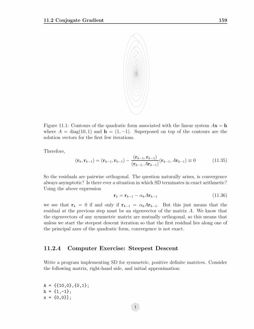
11.2 Conjugate Gradient 159
Figure 11.1: Contours of the quadratic form associated with the linear system Ax = hwhere A = diag(10, 1) and h = (1,−1). Superposed on top of the contours are thesolution vectors for the first few iterations.
Therefore,
(rk, rk−1) = (rk−1, rk−1)−(rk−1, rk−1)
(rk−1, Ark−1)(rk−1, Ark−1) ≡ 0 (11.35)
So the residuals are pairwise orthogonal. The question naturally arises, is convergencealways asymptotic? Is there ever a situation in which SD terminates in exact arithmetic?Using the above expression
rk = rk−1 − αkArk−1 (11.36)
we see that rk = 0 if and only if rk−1 = αkArk−1. But this just means that theresidual at the previous step must be an eigenvector of the matrix A. We know thatthe eigenvectors of any symmetric matrix are mutually orthogonal, so this means thatunless we start the steepest descent iteration so that the first residual lies along one ofthe principal axes of the quadratic form, convergence is not exact.
11.2.4 Computer Exercise: Steepest Descent
Write a program implementing SD for symmetric, positive definite matrices. Considerthe following matrix, right-hand side, and initial approximation:
A = 10,0,0,1;
h = 1,-1;
x = 0,0];
1

160 Iterative Linear Solvers
Symbolic arithmetic packages, including Mathematica, can solve the problem in exactarithmetic. This is very useful for analysis of the effects of rounding errors.
Figure out geometrically what steepest descent is doing. Does SD ever converge infinitely many steeps on this problem in exact arithmetic? In this case you should beable to derive an analytic expression for the residual vector. Make plots showing thelevel curves of the quadratic form associated with A. Then plot the solution vector asa function of iteration. The changes should always be normal to the contours. Underwhat circumstances can the residual vector be exactly zero? What is the geometricalinterpretation of this?
Do your conclusions generalize to symmetric non-diagonal matrices?
What happens if you change the matrix from diag(10,1) to diag(100,1)?
11.2.5 The Method of Conjugate Directions
The problem with steepest descent (SD) is that for ill-conditioned matrices the residualvector doesn’t change much from iteration to iteration. A simple scheme for improvingits performance goes back to Fox, Husky, and Wilkinson [FHW49] and is called theconjugate direction (CD) method. Instead of minimizing along the residual vector, asin SD, minimize along “search vectors” pk which are assumed (for now) to be orthogonalwith respect to the underlying matrix. This orthogonality will guarantee convergenceto the solution in at most n steps, where n is the order of the matrix.
So replace the step
xk = xk−1 + αkrk−1
with
xk = xk−1 + αkpk−1
where p is to be defined. As in SD the idea is to minimize f along these lines. The scalefactors α, as in SD, are determined by the minimization. Using the proof of Lemma 2,
f(xk + αpk) = f(xk) +1
2(αpk, Aαpk)− (αpk, rk) (11.37)
= f(xk) +1
2α2(pk, Apk)− α(pk, rk)
Setting ∂f(xk+αpk)∂α
= 0 gives
α ≡ αk+1 =(pk, rk)
(pk, Apk)=
(rk, rk)
(pk, Apk).
The last expression for α is part of Lemma 4
1

11.2 Conjugate Gradient 161
So, provided the scale factors αk satisfy the last equation, one is guaranteed to minimizethe residual along the search vector pk. The conditions necessary for the search vectorsare given by the following theorem.
Theorem 14 Conjugate Direction Theorem Suppose that the search vectors arechosen such that (pi, Apj) = 0 if i 6= j (A-orthogonality), then the CD method convergesto the exact solution in at most n steps.
Proof. Using the CD iteration
xk = xk−1 + αkpk−1, k = 1, 2, . . .
one has by induction
xk − x0 = α1p0 + α2p1 + · · ·+ αkpk−1
for any x0 chosen. Since the p vectors are A-orthogonal, it follows that
(pk, A(xk − x0)) = 0.
The A-orthogonality also implies that the p vectors must be linearly independent. Thusany vector in Rn can be represented as an expansion in the pkn−1
k=0. In particular, theunknown solution z of the linear system can be written
z = γ0p0 + · · ·+ γn−1pn−1.
Taking the inner product of this equation with first A and then pi, and using theA-orthogonality gives
(pi, Az) = γi(pi, Api)⇒ γi =(pi, Az)
(pi, Api).
The idea of the proof is to show that these numbers, namely the γi, are precisely thecoefficients of the CD algorithm; that would automatically yield convergence since byproceeding with CD we would construct this expansion of the solution. Just as anarbitrary vector x can be expanded in terms of the linearly independent search vectors,so can z− x0 where x0 is still the initial approximation. Thus,
z− x0 =n−1∑
i=0
(pi, A(z− x0))
(pi, Api)pi ≡
n−1∑
i=0
ξipi (11.38)
where
ξk =(pk, A(z− x0))
(pk, Apk). (11.39)
1

162 Iterative Linear Solvers
It was shown above that (pk, A(xk − x0)) = 0. Therefore one can subtract
(pk, A(xk − x0))/(pk, Apk)
from the expression for ξk without changing it. Thus,
ξk =(pk, A(z− x0))
(pk, Apk)− (pk, A(xk − x0))
(pk, Apk)
=(pk, A(z− xk))
(pk, Apk)
=(pk, rk)
(pk, Apk).
This is precisely the scale factor αk used in the CD iterations, which completes theproof. Thus we have
Algorithm 5 Method of Conjugate Directions Choose x0. This gives r0 = h −Ax0. Let piNi=1 be a set of A-orthogonal vectors. Then for k = 1, 2, 3, . . .
αk = (rk−1, rk−1)/(pk−1, Apk−1),xk = xk−1 + αkpk−1
rk = h− Axk
(11.40)
The A-orthogonality can be seen to arise geometrically from the fact that the vectorwhich points from the current location x to the global minimum of the quadratic formz must be A-orthogonal to the tangent plane of the quadratic form. To see this observethat since since the residual r must be normal to the surface, a tangent t must satisfy(t, r) = 0. Therefore 0 = (t, Ax− h) = (t, Ax− Az) = (t, Ap), where p = x− z.
So far, all this shows is that if n vectors, orthogonal with respect to the matrix Acan be found, then the conjugate direction algorithm will give solutions to the linearsystems of the matrix. One can imagine applying a generalized form of Gram-Schmidtorthogonalization to an arbitrary set of linearly independent vectors. In fact Hestenesand Stiefel [HS52] show that A-orthogonalizing the n unit vectors in Rn and usingthem in CD leads essentially to Gaussian elimination. But this is no real solution sinceGram-Schmidt requires O(n3) operations, and the search vectors, which will generallybe dense even when the matrix is sparse, must be stored. The real advance to CD wasmade by Hestenes and Stiefel, who showed that A-orthogonal search vectors could becomputed on the fly. This is the conjugate gradient method.
11.2.6 The Method of Conjugate Gradients
Using the machinery that has been developed, it is a relatively easy task to describethe conjugate gradient (CG) algorithm as originally proposed by Hestenes and Stiefel
1
11.2 Conjugate Gradient 163
[HS52].c In going from steepest descent to conjugate directions, minimization along theresiduals was replaced by minimization along the search vectors. So it makes sense toconsider computing the search vectors iteratively from residuals. Suppose we make theansatz p0 = r0 and
pk+1 = rk+1 + βk+1pk. (11.41)
Can the coefficients β be chosen so as to guarantee the A-orthogonality of the p vectors?Using (11.41), one has
(pk, Apk+1) = (pk, Ark+1) + βk+1(pk, Apk). (11.42)
If one chooses
βk+1 = −(pk, Ark+1)
(pk, Apk)
then the A-orthogonality is guaranteed. In Lemma 4 it will be shown that
βk+1 = −(rk+1, Apk)
(pk, Apk)=
(rk+1, rk+1)
(rk, rk)
As a final touch, notice that the residuals can be calculated recursively; by induction
rk+1 ≡ h− Axk+1
= h− A(xk + αk+1pk)
= (h− Axk)− αk+1Apk
= rk − αk+1Apk.
The result of all this work is:
Algorithm 6 Method of Conjugate Gradients Choose x0. Put p0 = r0 = h−Ax0.Then for k = 0, 1, 2, . . .
αk+1 = (rk,rk)(pk ,Apk)
xk+1 = xk + αk+1pkrk+1 = rk − αk+1Apkβk+1 = (rk+1,rk+1)
(rk,rk)
pk+1 = rk+1 + βk+1pk
(11.43)
The α coefficients are the same as in the CD algorithm, whereas the β coefficients arisefrom the CG ansatz: p0 = r0,pk+1 = rk+1 + βk+1pk. From a computational point ofview, note the simplicity of the algorithm. It involves nothing more than:
• The inner product of a matrix and a vector; and only one per iteration since Apkcan be calculated once and stored.
cThe method was invented independently by M. Hestenes [Hes51] and E. Stiefel [Sti52], who latercollaborated on the famous paper of 1952.
1
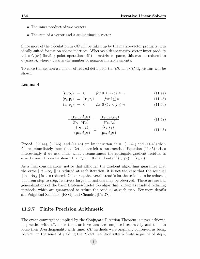
164 Iterative Linear Solvers
• The inner product of two vectors.
• The sum of a vector and a scalar times a vector.
Since most of the calculation in CG will be taken up by the matrix-vector products, it isideally suited for use on sparse matrices. Whereas a dense matrix-vector inner producttakes O(n2) floating point operations, if the matrix is sparse, this can be reduced toO(nzero), where nzero is the number of nonzero matrix elements.
To close this section a number of related details for the CD and CG algorithms will beshown.
Lemma 4
(ri,pj) = 0 for 0 ≤ j < i ≤ n (11.44)
(ri,pi) = (ri, ri) for i ≤ n (11.45)
(ri, rj) = 0 for 0 ≤ i < j ≤ n (11.46)
−(rk+1, Apk)
(pk, Apk)=
(rk+1, rk+1)
(rk, rk)(11.47)
(pk, rk)
(pk, Apk)=
(rk, rk)
(pk, Apk)(11.48)
Proof. (11.44), (11.45), and (11.46) are by induction on n. (11.47) and (11.48) thenfollow immediately from this. Details are left as an exercise. Equation (11.45) arisesinterestingly if we ask under what circumstances the conjugate gradient residual isexactly zero. It can be shown that ri+1 = 0 if and only if (ri,pi) = (ri, ri).
As a final consideration, notice that although the gradient algorithms guarantee thatthe error ‖ z − xk ‖ is reduced at each iteration, it is not the case that the residual‖ h−Axk ‖ is also reduced. Of course, the overall trend is for the residual to be reduced,but from step to step, relatively large fluctuations may be observed. There are severalgeneralizations of the basic Hestenes-Stiefel CG algorithm, known as residual reducingmethods, which are guaranteed to reduce the residual at each step. For more detailssee Paige and Saunders [PS82] and Chandra [Cha78].
11.2.7 Finite Precision Arithmetic
The exact convergence implied by the Conjugate Direction Theorem is never achievedin practice with CG since the search vectors are computed recursively and tend toloose their A-orthogonality with time. CD methods were originally conceived as being“direct” in the sense of yielding the “exact” solution after a finite sequence of steps,
1

11.2 Conjugate Gradient 165
the number of which was known in advance. It soon became apparent that CG couldbe used as an iterative method. One can show that [Cha78]:
‖ x− xk ‖A≤‖ x− x0 ‖A(
1−√κ1 +√κ
)2k
(11.49)
where κ ≡ λmax/λmin is the condition number of the matrix and ‖ x ‖A≡√
(x, Ax). If
the condition number is very nearly one, then (1−√κ)/(1 +√κ) is very small and the
iteration converges rapidly. On the other hand if κ = 105 it may take several hundrediterations to get a single digit’s improvement in the solution. But (11.49) is only anupper bound and probably rather pessimistic unless the eigenvalues of the matrix arewell separated. For some problems, a comparatively small number of iterations willyield acceptable accuracy. And in any event, the convergence can be accelerated by atechnique known as preconditioning.
The idea behind preconditioning is to solve a related problem having a much smallercondition number, and then transform the solution of the related problem into the oneyou want. If one is solving Ax = h, then write this instead as
Ax = h (11.50)
AC−1Cx = h
A′x′ = h
where A′ ≡ AC−1 and Cx ≡ x′. To be useful, it is necessary that
• κ(A′) κ(A)
• Cx = h should be easily solvable.
In this case, CG will converge much more rapidly to a solution of A′x′ = h than ofAx = h and one will be able to recover x by inverting Cx = x′. Alternatively, onecould write the preconditioned equations as
Ax = h (11.51)
DAx = Dh
A′x = h′
where DA ≡ A′ and Dh ≡ h′.
The most effective preconditioner would be the inverse of the original matrix, sincethen CG would converge in a single step. At the other extreme, the simplest precondi-tioner from a computational standpoint would be a diagonal matrix; whether any usefulpreconditioning can be obtained from so simple a matrix is another matter. Betweenthese two extremes lies a vast array of possible methods many of which are based uponan approximate factorization of the matrix. For example one could imagine doing a
1

166 Iterative Linear Solvers
Cholesky decomposition of the matrix and simply throwing away any nonzero elementswhich appear where the original matrix had a zero. In other words, one could en-force the sparsity pattern of A on its approximate factorization. For details on these“incomplete factorization” methods see [Man80],[Ker78], and [GvL83], for example.
11.2.8 CG Methods for Least-Squares
Conjugate gradient can be extended to the least squares solution of arbitrary linearsystems. Solutions of the normal equations
ATAx = ATh (11.52)
are critical points of the function
‖ Ax− h ‖2≡ ((Ax− h), (Ax− h)). (11.53)
Note that ATA is always symmetric and nonnegative. The basic facts for least-squaressolutions are these: if the system Ax = h is overdetermined, i.e., if there are more rowsthan columns, and if the columns are linearly independent, then there is a unique least-squares solution. On the other hand, if the system is underdetermined or if some of thecolumns are linearly dependent then the least-squares solutions are not unique. (For acomplete discussion see the book by Campbell and Meyer [CM79].) In the latter case,the solution to which CG converges will depend on the initial approximation. Hestenes[Hes75] shows that if x0 = 0, the usual case, then CG converges to the least-squaressolution of smallest Euclidean norm.
In applying CG to the normal equations avoid explicitly forming the products ATA.This is because the matrix ATA is usually dense even when A is sparse. But CG doesnot actually require the matrix, only the action of the matrix on arbitrary vectors. Soone could imagine doing the matrix-vector vector multiplies ATAx by first doing Ax andthen dotting AT into the resulting vector. Unfortunately, since the condition numberof ATA is the square of the condition number of A, this results in slowly convergentiteration if κ(A) is reasonably large. The solution to this problem is contained, onceagain, in Hestenes’ and Stiefel’s original paper [HS52]. The idea is to apply CG to thenormal equations, but to factor terms of the form ATh−ATAx into AT (h−Ax), doingthe subtraction before the final matrix multiplication. The result is
Algorithm 7 Conjugate Gradient Least Squares (CGLS) Choose x0. Put s0 =
1
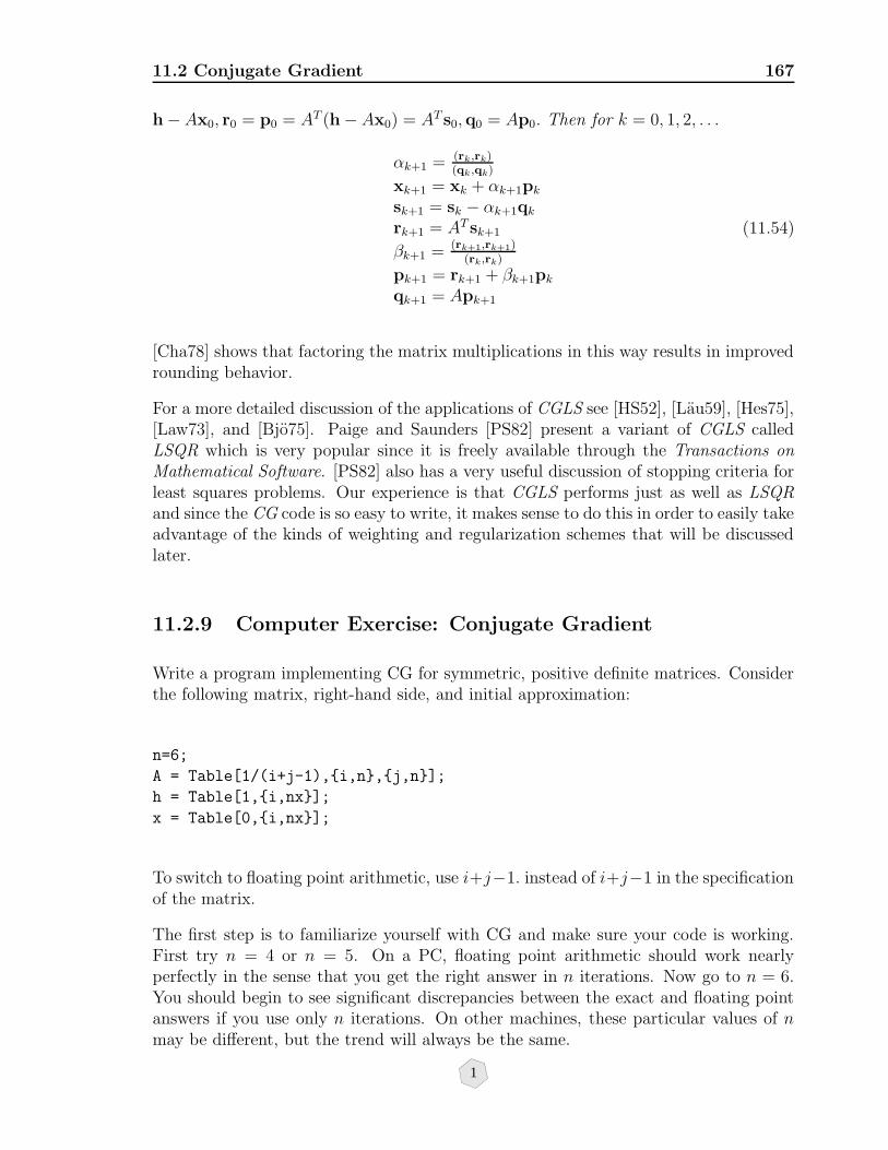
11.2 Conjugate Gradient 167
h− Ax0, r0 = p0 = AT (h− Ax0) = AT s0,q0 = Ap0. Then for k = 0, 1, 2, . . .
αk+1 = (rk ,rk)(qk ,qk)
xk+1 = xk + αk+1pksk+1 = sk − αk+1qkrk+1 = AT sk+1
βk+1 = (rk+1,rk+1)(rk,rk)
pk+1 = rk+1 + βk+1pkqk+1 = Apk+1
(11.54)
[Cha78] shows that factoring the matrix multiplications in this way results in improvedrounding behavior.
For a more detailed discussion of the applications of CGLS see [HS52], [Lau59], [Hes75],[Law73], and [Bjo75]. Paige and Saunders [PS82] present a variant of CGLS calledLSQR which is very popular since it is freely available through the Transactions onMathematical Software. [PS82] also has a very useful discussion of stopping criteria forleast squares problems. Our experience is that CGLS performs just as well as LSQRand since the CG code is so easy to write, it makes sense to do this in order to easily takeadvantage of the kinds of weighting and regularization schemes that will be discussedlater.
11.2.9 Computer Exercise: Conjugate Gradient
Write a program implementing CG for symmetric, positive definite matrices. Considerthe following matrix, right-hand side, and initial approximation:
n=6;
A = Table[1/(i+j-1),i,n,j,n];
h = Table[1,i,nx];
x = Table[0,i,nx];
To switch to floating point arithmetic, use i+j−1. instead of i+j−1 in the specificationof the matrix.
The first step is to familiarize yourself with CG and make sure your code is working.First try n = 4 or n = 5. On a PC, floating point arithmetic should work nearlyperfectly in the sense that you get the right answer in n iterations. Now go to n = 6.You should begin to see significant discrepancies between the exact and floating pointanswers if you use only n iterations. On other machines, these particular values of nmay be different, but the trend will always be the same.
1

168 Iterative Linear Solvers
Try to assess what’s going on here in terms of the numerical loss of A-orthogonality ofthe search vectors. You’ll need to do more than look at adjacent search vectors. Youmight try comparing p0 with all subsequent search vectors.
Now see if you can fix this problem simply by doing more iterations. If you get theright answer ultimately, why? What are the search vectors doing during these extraiterations. This is a subtle problem. Don’t be discouraged if you have trouble comingup with a compelling answer.
Are the residuals monotonically decreasing? Should they be?
What’s the condition number of the matrix for n = 6?
11.3 Practical Implementation
11.3.1 Sparse Matrix Data Structures
Clearly one needs to store all of the nonzero elements of the sparse matrix and enoughadditional information to be able to unambiguously reconstruct the matrix. But thesetwo principles leave wide latitude for data structures.d It would seem that the moresophisticated a data structure, and hence the more compact its representation of thematrix, the more difficult are the matrix operations. Probably the simplest scheme isto store the row and column indices in separate integer arrays. Calling the three arrayselem (a real array containing the nonzero elements of A), irow and icol, one has
elem(i) = A(irow(i), icol(i)) i = 1, 2, . . . , NZ (11.55)
where NZ is the number of nonzero elements in the matrix. Thus if the matrix is
1 0 0 43 −2 0 00 0 −1 0
then elem = (1, 4, 3,−2,−1), irow = (1, 1, 2, 2, 3), and icol = (1, 4, 1, 2, 3). The storagerequirement for this scheme is nzero real words plus 2 × nzero integer words. Butclearly there is redundant information in this scheme. For example, instead of storingall of the row indices one could simply store a pointer to the beginning of each newrow within elem. Then irow would be (1, 3, 5, 6). The 6 is necessary so that one knowshow many nonzero elements there are in the last row of A. The storage requirement forthis scheme (probably the most common in use) is nzero real words plus nzero+nrowinteger words, where nrow is the number of rows in A. In the first scheme, call it the
dA well-written and thorough introduction to sparse matrix methods is contained in Serge Pissanet-sky’s book Sparse Matrix Technology [Pis84].
1
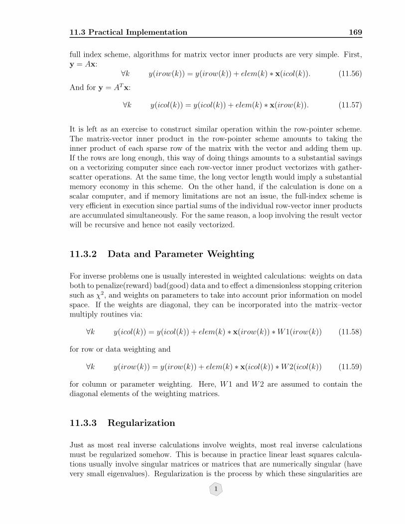
11.3 Practical Implementation 169
full index scheme, algorithms for matrix vector inner products are very simple. First,y = Ax:
∀k y(irow(k)) = y(irow(k)) + elem(k) ∗ x(icol(k)). (11.56)
And for y = ATx:
∀k y(icol(k)) = y(icol(k)) + elem(k) ∗ x(irow(k)). (11.57)
It is left as an exercise to construct similar operation within the row-pointer scheme.The matrix-vector inner product in the row-pointer scheme amounts to taking theinner product of each sparse row of the matrix with the vector and adding them up.If the rows are long enough, this way of doing things amounts to a substantial savingson a vectorizing computer since each row-vector inner product vectorizes with gather-scatter operations. At the same time, the long vector length would imply a substantialmemory economy in this scheme. On the other hand, if the calculation is done on ascalar computer, and if memory limitations are not an issue, the full-index scheme isvery efficient in execution since partial sums of the individual row-vector inner productsare accumulated simultaneously. For the same reason, a loop involving the result vectorwill be recursive and hence not easily vectorized.
11.3.2 Data and Parameter Weighting
For inverse problems one is usually interested in weighted calculations: weights on databoth to penalize(reward) bad(good) data and to effect a dimensionless stopping criterionsuch as χ2, and weights on parameters to take into account prior information on modelspace. If the weights are diagonal, they can be incorporated into the matrix–vectormultiply routines via:
∀k y(icol(k)) = y(icol(k)) + elem(k) ∗ x(irow(k)) ∗W1(irow(k)) (11.58)
for row or data weighting and
∀k y(irow(k)) = y(irow(k)) + elem(k) ∗ x(icol(k)) ∗W2(icol(k)) (11.59)
for column or parameter weighting. Here, W1 and W2 are assumed to contain thediagonal elements of the weighting matrices.
11.3.3 Regularization
Just as most real inverse calculations involve weights, most real inverse calculationsmust be regularized somehow. This is because in practice linear least squares calcula-tions usually involve singular matrices or matrices that are numerically singular (havevery small eigenvalues). Regularization is the process by which these singularities are
1

170 Iterative Linear Solvers
tamed. We saw two different examples of regularization in Chapter 5. The first wastruncating the SVD. We can throw away zero or small singular values and that regu-larizes the problem. But we also found that in the presence of a model null space itwas useful to be able to penalize the size of the solution as well as the data misfit.
In other words we replaced the minimization problem
min ‖ Ax− h ‖2 (11.60)
with
min ‖ Ax− h ‖2 + ‖ x ‖2 . (11.61)
The first term is the data misfit, and the second is the “regularization” term. As shownhere, the two aspects of the minimization (make the data misfit small, make the modelnorm small) get equal weight.
Now let us go two steps beyond this. First, let us introduce a fudge factor λ to controlthe tradeoff between the two terms. Next, let us consider the possibility of minimizingnot the norm of the model itself, but the norm of some linear function of the modelRh.
min ‖ Ax− h ‖2 +λ ‖ Rx ‖2 (11.62)
If R = I, then we’re back to our familiar regularization. But now suppose that R ≡∂n, n = 0, 1, 2, . . . and ∂n is an n− th order discrete difference operator. In this case theterm ‖ Rx ‖2 penalizes the slope, roughness, or higher order derivative of the model.Penalizing roughness would be useful if we want a smooth solution.
The “normal equations” associated with this generalized objective function, obtainedby setting the derivative of (11.62) equal to zero, are
(ATA + λRTR)x = ATh. (11.63)
This sort of regularization is straightforward to implement in a sparse matrix frameworkby augmenting the matrix with the regularization term:
A ≡(
A√λR
).
From this you can tell right away that R must have the same number of columns as A.But in principle it can have any number of rows. For example, we might use
R =
1 −1 0 · · ·0 1 −1 · · ·
...0 · · · 1 −10 0 · · · 1
1
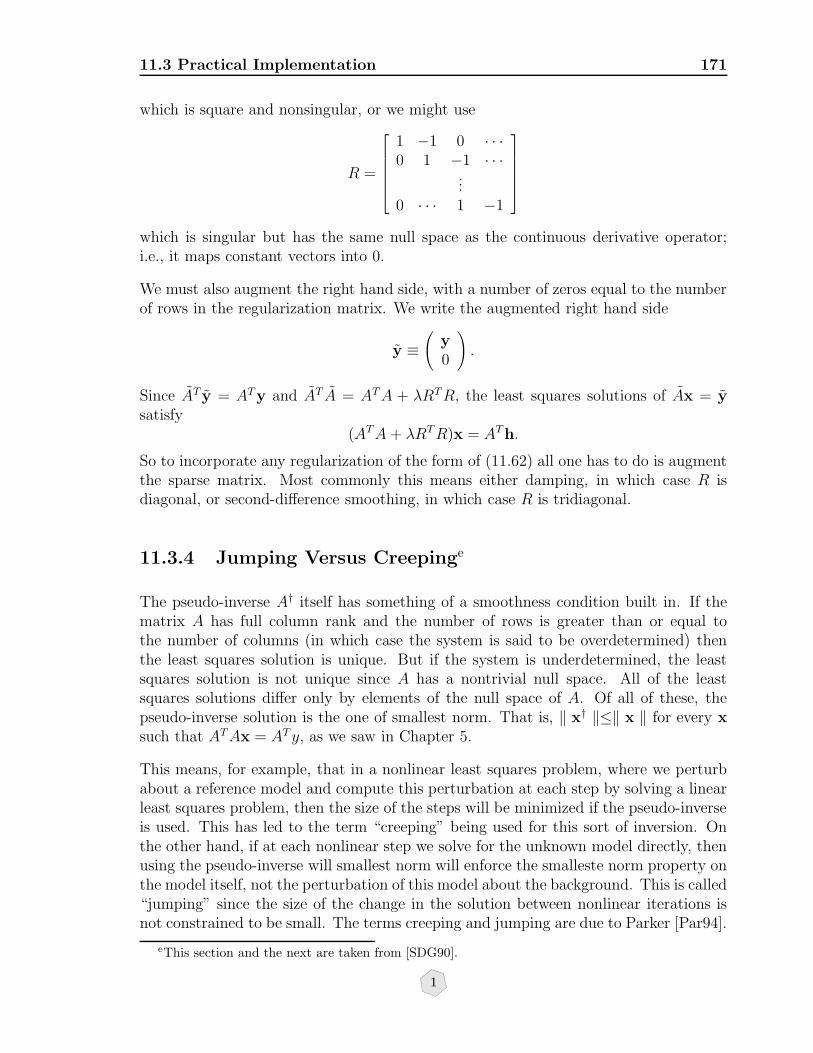
11.3 Practical Implementation 171
which is square and nonsingular, or we might use
R =
1 −1 0 · · ·0 1 −1 · · ·
...0 · · · 1 −1
which is singular but has the same null space as the continuous derivative operator;i.e., it maps constant vectors into 0.
We must also augment the right hand side, with a number of zeros equal to the numberof rows in the regularization matrix. We write the augmented right hand side
y ≡(
y0
).
Since AT y = ATy and AT A = ATA + λRTR, the least squares solutions of Ax = ysatisfy
(ATA + λRTR)x = ATh.
So to incorporate any regularization of the form of (11.62) all one has to do is augmentthe sparse matrix. Most commonly this means either damping, in which case R isdiagonal, or second-difference smoothing, in which case R is tridiagonal.
11.3.4 Jumping Versus Creepinge
The pseudo-inverse A† itself has something of a smoothness condition built in. If thematrix A has full column rank and the number of rows is greater than or equal tothe number of columns (in which case the system is said to be overdetermined) thenthe least squares solution is unique. But if the system is underdetermined, the leastsquares solution is not unique since A has a nontrivial null space. All of the leastsquares solutions differ only by elements of the null space of A. Of all of these, thepseudo-inverse solution is the one of smallest norm. That is, ‖ x† ‖≤‖ x ‖ for every xsuch that ATAx = ATy, as we saw in Chapter 5.
This means, for example, that in a nonlinear least squares problem, where we perturbabout a reference model and compute this perturbation at each step by solving a linearleast squares problem, then the size of the steps will be minimized if the pseudo-inverseis used. This has led to the term “creeping” being used for this sort of inversion. Onthe other hand, if at each nonlinear step we solve for the unknown model directly, thenusing the pseudo-inverse will smallest norm will enforce the smalleste norm property onthe model itself, not the perturbation of this model about the background. This is called“jumping” since the size of the change in the solution between nonlinear iterations isnot constrained to be small. The terms creeping and jumping are due to Parker [Par94].
eThis section and the next are taken from [SDG90].
1
172 Iterative Linear Solvers
This point merits a brief digression since the effects of damping or smoothing will bedifferent according as one is doing jumping or creeping. Suppose the nonlinear inverseproblem is: given y, find x such that y− F (x) is minimized in some sense. Expandingthe forward problem F to first order in a Taylor series about some model x0 gives
y = y0 + F ′(x0)(x− x0) (11.64)
where y0 ≡ F (x0). Denoting the Jacobian F ′ by A, there are two alternative leastsquares solutions of the linearized equations
Jumping xj = A†(Ax0 + y− y0) (11.65)
Creeping xc = x0 + A†(y− y0) (11.66)
differing only in how the pseudo-inverse is applied.
In creeping x− x0 is a minimum norm least squares solution of the linearized forwardequations, whereas in jumping the updated model x is itself a minimum norm leastsquares solution. The difference between the jumping and creeping (in the absence ofregularization) is readily seen to be
xj − xc = (A†A− I)x0. (11.67)
Expressing the initial model in terms of its components in the row space and null spaceof A,
x0 = xrow0 + xnull0 (11.68)
and noting that
xrow0 = A†Ax0 (11.69)
then
xj = xrow0 + A†(y − y0) (11.70)
and (11.67) becomes
xj − xc = −xnull0 . (11.71)
Thus, the creeping and jumping solutions differ by the component of the initial modelthat lies in the null space of A: some remnants of the initial model that appear in xc
are not present in xj. Only if A is of full column rank (giving A†A = I ) will the twosolutions be the same for any initial guess. In the next sections it will be seen that thisanalysis must be modified when regularization is employed.
11.3.5 How Smoothing Affects Jumping and Creeping
In the absence of regularization, the jumping and creeping solutions differ only by thecomponent of the initial model in the null space of the Jacobian matrix. Regulariza-tion changes things somewhat since the matrix associated with the regularized forward
1

11.3 Practical Implementation 173
problem has no nontrivial null space. Recall that for jumping, the linearized problem,with solution xj, is
Axj = Ax0 + y − y0 (11.72)
whereas for creepingA(xc − x0) = y − y0. (11.73)
The addition of regularization produces the augmented systems
Axj =
(y− y0 + Ax0
0
)(11.74)
and
A(xc − x0) =
(y − y0
0
). (11.75)
Inverting, one has
xj = A†(
y − y0 + Ax0
0
)= A†
(y − y0
0
)+ A†
(Ax0
0
). (11.76)
and
xc − x0 = A†(
y − y0
0
). (11.77)
Thus
xj − xc = A†(Ax0
0
)− x0. (11.78)
For λ > 0 the augmented matrix is nonsingular,f therefore one can write
x0 = A†Ax0.
Using the definition of A
x0 = A†(
A√λR
)x0 = A†
(Ax0
0
)+ A†
(0√λRx0
). (11.79)
Finally from (11.78) and (11.79) one obtains
xj − xc = −A†(
0√λRx0
). (11.80)
As in (11.71), the difference between the two solutions depends on the initial model.But when smoothing is applied, the creeping solution possesses components related tothe slope of x0 (first difference smoothing) or to the roughness of x0 (second differencesmoothing) which are not present in the jumping solution. An important corollary ofthis result is that for smooth initial models, jumping and creeping will give the sameresults when roughness penalties are employed to regularize the calculation. Exam-ples illustrating the comparative advantages of jumping and creeping are contained in[SDG90].
fIf the columns of the regularization operator are linearly independent, then the columns of theaugmented matrix are too.
1
174 Iterative Linear Solvers
11.4 Sparse Singular Value Calculationsg
The singular value decomposition is one of the most useful items in the inverter’stoolkit. With the SVD one can compute the pseudo-inverse solution of rectangularlinear systems, analyze resolution (within the linear and Gaussian assumptions), studythe approximate null space of the forward problem, and more. The now classical Golub-Reinsch approach to SVD [GR70] begins by reducing the matrix to block bidiagonalform via a sequence of transformations known as Householder transformations. TheHouseholder transformations annihilate matrix elements below the diagonal, one col-umn at a time. Unfortunately, after each transformation has been applied, the sparsitypattern in the remaining lower triangular part of the matrix is the union of the sparsitypattern of the annihilated column and the rest of the matrix. After a very few steps,one is working with nearly full intermediate matrices. This makes conventional SVDunsuitable for large, sparse calculations. On the other hand, for some problems, suchas studying the approximate null space of the forward problem, one doesn’t really needthe entire SVD; it suffices to compute the singular vectors associated with the smallsingular values (“small” here is defined relative the level of noise in the data). Or per-haps from experience one knows that one must iterate until all those eigenvectors downto a certain eigenvalue level have been included in the solution. Conventional SVDgives no choice in this matter, it’s all or nothing. In this section we shall consider theuse of iterative methods such as conjugate gradient for computing some or all singularvalue/singular vector pairs.
11.4.1 The Symmetric Eigenvalue Problem
For convenience (actually, to be consistent with the notation in [Sca89]) here is anequivalent form of the CG algorithm for symmetric, positive-definite systems Ax = y.
Algorithm 8 Method of Conjugate Gradients Let x0 = 0, r0 = p1 = y andβ1 = 0. Then for i = 1, 2, . . .
βi = (ri−1,ri−1)(ri−2,ri−2)
pi = ri−1 + βipi−1
αi = (ri−1,ri−1)(pi,Api)
xi = xi−1 + αipiri = ri−1 − αiApi
(11.81)
Now define two matrices Rk and Pk whose columns are, respectively, the residual andsearch vectors at the k− th step of CG; Rk = (r0, . . . , rk−1) and Pk = (p1, . . . ,pk). LetBk be the bidiagonal matrix with ones on the main diagonal and (−βi, i = 2, . . . , k)
gThis section is based upon [Sca89]
1

11.4 Sparse SVD 175
on the superdiagonal (βi are the CG scale factors). Finally, let ∆k be the matrixdiag(ρ0, . . . , ρk−1), where ρi ≡‖ ri ‖.
Using the recursionpi+1 = ri + βi+1pi i = 2, . . . , k
and the fact that p1 = r0, it follows by direct matrix multiplication that
Rk = PkBk.
ThereforeRk
TARk = BkTPk
TAPkBk.
The reason for looking at RkTARk is that since Rk is orthogonal (cf. Lemma 4), the
matrix RkTARk must have the same eigenvalues as A itself.
But since the p vectors are A-orthogonal, it follows that
PkTAPk = diag[(p1, Ap1), . . . , (pk, Apk)].
Using this and normalizing the R matrix with ∆ gives the following tridiagonalizationof A
Tk = ∆k−1Bk
Tdiag[(p1, Ap1), . . . , (pk, Apk)]Bk∆k−1. (11.82)
Carrying through the matrix multiplications gives the elements of Tk
(Tk)i,i =
[1
αi+
βiαi−1
i = 1, . . . , k
](11.83)
(Tk)i,i+1 = (Tk)i+1,i =
[−√βi+1
αii = 1, . . . , k − 1
](11.84)
In other words, just by doing CG one gets a symmetric tridiagonalization of the matrixfor free. Needless to say, computing the eigenvalues of a symmetric tridiagonal matrixis vastly simpler and less costly than extracting them from the original matrix. Forrectangular matrices, simply apply the least squares form of CG and use the α and βscale factors in (11.83) and (11.84), to get a symmetric tridiagonalization of the normalequations. Then, just take their positive square roots to get the singular values. Thecalculation of the eigenvalues of symmetric tridiagonal matrices is the subject of a ratherlarge literature. See [Sca89] for details.
The following example illustrates the idea of iterative eigenvalue computation. We willconsider the Hilber matrix, whose i − j element is 1
i+j+1. This matrix arises in the
theory of approximation and is known to be highly ill-conditioned.h
The matrix in question is an eighth-order Hilbert matrix:
hA simple explanation for this was contributed to the Usenet news group sci.math by Zdislav V.Kovarik. The idea is you can interpret the i − j element as the inner product of xi and xj on theinterval [0, 1]. Now, the cosine of the angle between xk and x(k+ 1) is just 1
2∗k+2 . So you can see thatas k increases, this matrix. which consists of the scalar products of these almost linearly dependentvectors, is bound to be nearly singular.
1

176 Iterative Linear Solvers
nx =8;
A = Table[1/(i+j-1.),i,nx,j,nx];
The condition number of this matrix is 1010. The exact solution to the system Ax = y,where y consists of all ones is:
(−8, 504,−7560, 46200,−138600, 216216,−168168, 51480).
After just 5 iterations, using 16 digits of precision, CG produces the following solution:
(0.68320,−4.01647,−127.890, 413.0889,−19.3687,−498.515,−360.440, 630.5659)
which doesn’t look very promising. However, even after only 5 iterations we haveexcellent approximations to the first 4 eigenvalues. The progression towards theseeigenvalues is illustrated in the following table, which shows the fractional error in eacheigenvalue as a function of CG iterations. Even after only one iteration, we’ve alreadygot the first eigenvalue to within 12%. After 3 iterations, we have the first eigenvalueto within 1 part in a million and the second eigenvalue to within less than 1%.
Eigenvalue 1.6959389 0.2981252 0.0262128 0.0014676 0.0000543 IterationFractional 0.122 1
error in 0.015 0.52720 2CG-computed 1.0 10−5 0.006 1.284 3
eigenvalues 9.0 10−12 1.9 10−7 0.002 1.184 40.0 7.3 10−15 1.13 10−8 8.0 10−4 1.157 5
11.4.2 Finite Precision Arithmetic
Using CG or Lanczos methods to compute the spectrum of a matrix, rather than simplysolving linear systems, gives a close look at the very peculiar effects of rounding erroron these algorithms. Intuitively one might think that the main effects of finite preci-sion arithmetic would be a general loss of accuracy of the computed eigenvalues. Thisdoes not seem to be the case. Instead, “spurious” eigenvalues are calculated. Thesespurious eigenvalues fall into two categories. First, there are numerically multiple eigen-values; in other words duplicates appear in the list of computed eigenvalues. Secondly,and to a much lesser extent, there are extra eigenvalues. The appearance of spuriouseigenvalues is associated with the loss of orthogonality of the CG search vectors. Adetailed explanation of this phenomenon, which was first explained by Paige [Pai71] isbeyond the scope of this discussion. For an excellent review see ([CW85], Chapter 4).In practice, the duplicate eigenvalues are not difficult to detect and remove. Variousstrategies have been developed for identifying the extra eigenvalues. These rely eitheron changes in the T matrix from iteration to iteration (in other words, on changes inTm as m increases), or differences in the spectra between T (at a given iteration) andthe principle submatrix of T formed by deleting its first row and column. An extensive
1

11.4 Sparse SVD 177
discussion of the tests used for detecting spurious eigenvalues is given by [CW85]. It isalso not obvious how many iterations of CG are necessary to generate a given numberof eigenvalues. At best it appears that for “large enough [number of iterations] m, everydistinct eigenvalue of A is an eigenvalue of Tm”—the Lanczos phenomenon[CW80]. Onthe other hand, the spurious eigenvalues crop up because one has been content to letthe search vectors lose orthogonality: computing a lot of iterations, throwing away alot of duplicate eigenvalues, and relying on the Lanczos phenomenon to assure thateventually one will calculate all of the relevant eigenvalues. The examples in [CW85]and the example that will be shown presently would seem to indicate that that is notan unreasonable goal. On the other hand, many (perhaps most) practitioners of theLanczos method advocate some sort of partial or selective reorthogonalization. In otherwords, orthogonalize by hand the current search vector with respect to the last, say, Nvectors, which then must be stored. Some examples of reorthogonalized Lanczos aregiven by [Par80]. It is difficult to do justice to the controversy which surrounds thispoint; suffice it to say, whether one uses reorthogonalized methods or not, care must betaken to insure, on the one hand, that spurious eigenvalues are not mistakenly included,and on the other, that reorthogonalization is sufficiently selective that the speed of themethod is not completely lost.
Here is a simple example of the use of CG-tridiagonalization from [Sca89]. The problemis a small, 1500 or so rays, travel time inversion of reflection seismic data. The modelhas about 400 unknown elastic parameters. In the table below are listed the first 40singular values of the Jacobian matrix computed with an SVD (on a Cray X-MP) andusing Conjugate Gradient. Duplicate singular values have been removed. The resultsare extremely close except for the three spurious singular values 7, 24, and 38. In all Iwas able to compute about half of the nonzero singular values without difficulty. Mostof these were accurate to at least 6 or 7 decimal places.
1

178 Iterative Linear Solvers
SINGULAR VALUES SVD CG1 23.762031619755 23.76203161975670502 19.768328927112 19.76832892710781313 16.578534293957 16.57853429396164564 14.354045541174 14.35404554117357575 13.006121206565 13.00612120656864606 12.293303623664 12.29330362366727887 11.610930621056 12.15923027679064558 10.895471779225 11.61093062105453319 10.670981506845 10.895471779226897410 10.334874696665 10.670981506845439411 10.123412306695 10.334874696673731312 9.955310042953 10.123412306700557913 9.6454782226432 9.9553100429538792214 9.5529461513199 9.6454782226493129815 9.4273903010306 9.5529461513285911516 9.3371719187833 9.4273903010327284617 9.2486487219101 9.3371719187878961018 9.2020745407381 9.2486487219158706219 9.1365345361384 9.2020745407449910920 9.1105716770474 9.1365345361448160321 8.9573315416959 9.1105716770518634422 8.897862083302 8.9573315417023997623 8.6901794080491 8.8978620833082433524 8.6263321041541 8.8677090744391438025 8.3362097313284 8.6901794080581378226 8.253249495322 8.6263321041555518527 8.1701784446507 8.3362097313391594328 8.009740159019 8.2532494953281221329 7.9256810850057 8.1701784446558241030 7.8102692299697 8.0097401590299579531 7.6624515175111 7.9256810850050418732 7.5651235246644 7.8102692299672935633 7.348695068023 7.6624515175115932634 7.2070814800585 7.5651235246624151135 7.1082737154214 7.3486950680223988036 6.9528330413513 7.2070814800576636937 6.9267489577491 7.1082737154202491138 6.7567717799808 7.0539497539678146539 6.7316199620107 6.9528330413509125140 6.6700456432165 6.92674895774645272
1
11.4 Sparse SVD 179
11.4.3 Explicit Calculation of the Pseudo-Inverse
Finally, we point out a clever result of Hestenes which seems to have been largelyignored. In the paper [Hes75] he proves the following. Let r be the rank of A anarbitrary matrix, and let p and q be the CGLS search vectors, and let x0 = 0. Then
A† =
[p0p0
(q0,q0)+
p1p1
(q1,q1)+ · · · pr−1pr−1
(qr−1,qr−1)
]AT (11.85)
is the generalized pseudo-inverse of A. A generalized pseudo-inverse satisfies only twoof the four Penrose conditions, to wit:
A†AA† = A† (11.86)
AA†A = A (11.87)
To illustrate this result, consider the following least squares problem:
1 2−4 5−1 32 −7
[xy
]=
565−12
.
The column rank of the matrix is 2. It is straightforward to show that
[ATA
]−1=
1
689
[22 3535 87
].
Therefore the pseudo-inverse is
A† =[ATA
]−1AT =
1
689
[157 −173 18 −7179 −30 31 −84
].
Now apply the CGLS algorithm. The relevant calculations are
p0 =
[−48139
], q0 =
230887465−1069
.
p1 =
[9.976014.28871
], q1 =
18.55343−18.46049
2.89012−10.06985
, x2 =
[1.000002.00000
],
which is the solution. Recalling (11.85)
A† =
[p0p0
(q0,q0)+
p1p1
(q1,q1)+ · · · pr−1pr−1
(qr−1,qr−1)
]AT (11.88)
1
180 BIBLIOGRAPHY
one has [p0p0
(q0,q0)+
p1p1
(q1,q1)
]=
[0.12627 0.050800.05080 0.03193
].
But this is nothing more than[ATA
]−1which was previously calculated:
[ATA
]−1=
1
689
[22 3535 87
]=
[0.12627 0.050800.05080 0.03193
].
In this particular case A†A = I so the parameters are perfectly well resolved in theabsence of noise.
Exercises
1. Prove Equation (11.22).
2. Show that
f(z)− f(xk) = −1
2(xk − z, A(xk − z))
where z is a solution to Ax = h and A is a symmetric, positive definite matrix.
3. Prove Lemma 4.
4. With steepest descent, we saw that in order for the residual vector to be exactlyzero, it was necessary for the initial approximation to the solution to lie on oneof the principle axes of the quadratic form. Show that with CG, in order for theresidual vector to be exactly zero we require that
(ri,pi) = (ri, ri)
which is always true by virtue of Lemma 3.
Bibliography
[Bjo75] A. Bjork. Methods for sparse linear least-squares problems. In J. Bunch andD. Rose, editors, Sparse Matrix Computations. Academic, New York, 1975.
[Cha78] R. Chandra. Conjugate gradient methods for partial differential equations.PhD thesis, Yale University, New Haven, CT, 1978.
[CM79] S. Campbell and C. Meyer. Generalized inverses of linear transformations.Pitman, London, 1979.
[CW80] J. Cullum and R. Willoughby. The Lanczos phenomenon—an interpretationbased upon conjugate gradient optimization. Linear Albegra and Applica-tions, 29:63–90, 1980.
1
BIBLIOGRAPHY 181
[CW85] J. Cullum and R. Willoughby. Lanczos Algorithms for Large SymmetricEigenvalue Computations. Birkhauser, Boston, 1985.
[FHW49] L. Fox, H. Huskey, and J. Wilkinson. Notes on the solution of algebraic linearsimultaneous equations. Q. J. Mech. Appl. Math, 1:149–173, 1949.
[GR70] G. Golub and C. Reinsch. Singular value decomposition. Numerische Math.,14:403–420, 1970.
[GvL83] G. Golub and C. van Loan. Matrix Computations. Johns Hopkins, Baltimore,1983.
[Hes51] M. Hestenes. Iterative methods for solving linear equations. Technical report,National Bureau of Standards, 1951.
[Hes75] M. Hestenes. Pseudoinverses and conjugate gradients. Communications ofthe ACM, 18:40–43, 1975.
[HS52] M. Hestenes and E. Stiefel. Methods of conjugate gradients for solving linearsystems. NBS J. Research, 49:409–436, 1952.
[Ker78] D. Kershaw. The incomplete Cholesky-conjugate gradient method for theiterative solution of systems of linear equations. Journal of ComputationalPhysics, 26:43–65, 1978.
[Lau59] P. Lauchli. Iterative Losung und Fehlerabschatzung in der Ausgleichsrech-nung. Zeit. angew. Math. Physik, 10:245–280, 1959.
[Law73] C. Lawson. Sparse matrix methods based on orthogonality and conjugacy.Technical Report 33-627, Jet Propulsion Laboratory, 1973.
[Man80] T.A. Manteuffel. An incomplete factorization technique for positive definitelinear systems. Mathematics of Computation, 34:473–497, 1980.
[Pai71] C. Paige. The computation of eigenvalues and eigenvectors of very largesparse matrices. PhD thesis, University of London, London, England, 1971.
[Par80] B. Parlett. The Symmetric Eigenvalue Problem. Prentice-Hall, 1980.
[Par94] R.L. Parker. Geophysical Inverse Theory. Princeton University Press, 1994.
[Pis84] S. Pissanetsky. Sparse Matrix Technology. Academic, N.Y., 1984.
[PS82] C. Paige and M Saunders. LSQR: An algorithm for sparse linear equationsand sparse least squares. ACM Trans. Math. Softw., 8:43–71, 1982.
[SB80] J. Stoer and R. Bulirsch. Introduction to Numerical Analysis. Springer, N.Y.,1980.
1

182 BIBLIOGRAPHY
[Sca89] J.A. Scales. Using conjugate gradient to calculate the eigenvalues and singularvalues of large, sparse matrices. Geophysical Journal, 97:179–183, 1989.
[SDG90] J.A. Scales, P. Docherty, and A. Gersztenkorn. Regularization of nonlinearinverse problems: imaging the near-surface weathering layer. Inverse Prob-lems, 6:115–131, 1990.
[Sti52] E. Stiefel. Uber einige Methoden der Relaxationsrechnung. Zeit. angew.Math. Physik, 3, 1952.
[You71] D. M. Young. Iterative Solution of Large Linear Systems. Academic, N.Y.,1971.
1

Chapter 12
More on the Resolution-VarianceTradeoff
12.1 A Surfer’s Guide to Backus-Gilbert Theory
The basic reference is [BG67]. The standard discrete inverse problem is
d = Am + e (12.1)
where A is the derivative of the forward problem (an n by m matrix), m is a vector ofunknown model parameters, and d contains the observed data. m is a vector in Rm.However, it represents a discretization of the model slowness s(r), which is a scalarfunction defined on a closed subset Ω of RD, D ∈ (1, 2, 3 . . .). It will be assumed thatthe set of all possible models lies in some linear function space M.
It is useful to introduce an orthonormal basis of functions (we will use our oldfriends the pixel functions) which span the model space M. Suppose that Ω is com-pletely covered by m closed, convex, mutually disjoint sets (cells) σ ∈ RD : Ω = ∪ σisuch that σi ∩ σj = if i 6= j. The basis functions are then defined to be
hi(r) =
ν−1/2i if r ∈ σi
0 otherwise
where νi is the volume of the ith cell. The choice of the normalization ν−1/2i is made
to remove bias introduced by cell size. If a constant cell size is adopted, ν−1/2i can be
replaced with 1. Given the definition of hi, it is clear that∫
Ωhi(r)hj(r)dDr = δij.
Thus an arbitrary function can be written as an expansion in hi
m(r) =∞∑
i=1
mihi(r) ≡ m · h(r). (12.2)
1

184 More on the Resolution-Variance Tradeoff
In practice this sum will usually be truncated at a finite number of terms. For infinitedimensional vectors it is more traditional to write the inner product as (m,h(r)) butwe will continue to use the dot notation.
A basic took of BG theory is the point spread function A. The point spread function(PSF) is defined in a formal manner by noting that a local average of the model m(r) canbe obtained at any point r0 by integrating the model and a locally defined unimodularfunction
〈m(r0)〉 =∫
ΩA(r, r0)m(r)dDr. (12.3)
Unimodular means that the function integrates to 1.∫
ΩA(r, r0)dDr = 1.
Also, it is assumed that A(r, r0) ∈ M for each r0 ∈ Ω and that the support of A isconcentrated at the point r0. Naturally, the more accurately the model is determinedat each point, the more closely the PSF resembles a delta function – at that point. Soestimating the PSF is equivalent to estimating a local average of the model. The moredelta function-like is the PSF, the more precise our estimate of the model.
Like any other function in M, the PSF can be expanded in terms of hi.
A(r, r0) =∞∑
i=1
ai (r0) hi (r) ≡ a(r0) · h(r).
Thus (12.2) and (12.3) imply that
〈m(r0)〉 =∞∑
i=1
ai (r0)mi = a (r0) ·m. (12.4)
It is clear that one can construct a PSF which will yield a local average of the model– any approximation to a delta function will do. Unfortunately, there is a tradeoffbetween the sharpness of the PSF and the variance, or RMS error, of the solution. Toshow this, BG assume that the local average of the model is a linear function of thedata
〈m(r0)〉 =n∑
i=1
bi (r0) di = b (r0) · d = (b (r0) , Am + e) (12.5)
where b is to be determined. For the moment let’s neglect the noise–for zero meannoise we can just take expectations. Comparing (12.4) and (12.5) one sees that theexpansion coefficients of the PSF are simply
a (r0) = ATb (r0) (12.6)
Now, how one measures the “width” of the PSF is largely a matter of taste. Nolet[Nol85] makes the following natural choice
W (r0) = cD
∫
ΩA (r, r0)2 |r− r0|D+1 dDr
1

12.2 Using the SVD 185
where cD is a scale factor chosen to make W have as simple a form as possible. Forexample, Nolet chooses c3 = 56π/9. Plugging the definition of the pixel functions andof the PSF into (12.6) it follows that
W (r0) =∑
i,j,k
fiAjiAkibj (r) bk (r0) (12.7)
wherefi = cD
∫
Ω|r− r0|D+1 hi (r)2 dDr ≈ cD |ri − r0|D+1
and where ri is the centroid of the ith cell. Equation (12.7) shows how the width of thePSF depends on the b coefficients. Now all one needs is a similar expression for theerror of the average model value 〈m (r0)〉
σ2 = Var〈m (r0)〉 =n∑
i,j=1
bi (r0) bj (r0) Cov(di, dj) = b (r0) · b (r0) .
The last equality follows since if one assumes that the data are uncorrelated, thenweights can always be chosen such that Cov(di, dj) = δij. Thus, it has been shownthat both the width of the PSF and the variance of the solution depend on b; Thusone cannot tighten up the PSF without affecting the variance. The solution, at leastformally, is to introduce a tradeoff parameter, say w, and jointly minimize
J(w, r0) ≡ W (r0) + w2σ2(r0).
This last problem is straightforwardly solved but note that to compute the coefficientsb which jointly minimize the variance and the width of the PSF requires the solutionof a (large) least squares problem at each point in the model where the resolving poweris desired. For large, sparse operators A, a far more efficient approach would be usingthe conjugate gradient methods outlined in Chapter 11.
12.2 Using the SVD
Now let us look at this tradeoff for a finite-dimensional problem using the SVD. Let Abe the forward modeling operator, now assumed to map Rm to Rn:
d = Am + e
where e is an n-vector of random errors. The least squares estimated model m is givenby A†d, where A† is the pseudo-inverse of A.
The covariance of m is E[mmT ].a We can get a simple result for this matrix using thesingular value decomposition. The singular value decomposition of A is
A = UΛV T
aAssuming that the errors are zero mean since then E[m] = E[A†d] = A†E[d] = 0.
1

186 More on the Resolution-Variance Tradeoff
where U is an orthogonal matrix of “data” eigenvectors (i.e., they span Rn) and V isan orthogonal matrix of “model” eigenvectors (they span Rm). Λ is the n×m diagonalmatrix of singular values λi. The pseudo-inverse of A is
A† = V Λ−1UT
where Λ−1 where denotes the m×n diagonal matrix obtained by inverting the nonzerosingular values. To keep things simple, let’s assume that the covariance of the dataerrors is just the identity matrix. This will let us look at the structure of the covarianceof m as a function of the forward operator alone. It is easy to see that in this case
Cov(m) = E[mmT ] = A†Cov(d)A†T
= V Λ−2V T =m∑
i=1
λ−2i viv
Ti .
The last term on the right is the sum of the outer products of the columns of V(these are the model space eigenvectors). So the covariance can be seen as a weightedprojection operator onto the row space of A, with weights given by the inverse-squareof the singular values.
With this it is not difficult to see that the j-th diagonal element of Cov(m), which isthe variance of the j-th model parameter is
Var(mj) =m∑
i=1
λ−2i (vi)
2j
where (vi)j is the j-th component of the i-th eigenvector.
If the rank of A is less than m, say r, then all of the sums involving the pseudo-inverseare really only over the r eigenvectors/eigenvalues. In particular
Var(mj) =r∑
i=1
λ−2i (vi)
2j .
This is because A = UΛV T = UrΛrVTr where the subscript r means that we have
eliminated the terms associated with zero singular values.
Now suppose we decide not to use all the r model eigenvectors spanning the row spaceof A?b For example we might need only p eigenvectors to actually fit the data. Letus denote by mp the resulting estimate of m (which is obviously confined to the p-dimensional subspace of Rm spanned by the first p model singular vectors):
mp ≡p∑
i=1
viuTi d
λi
where ui is the i-th column of U (i.e., the i-th data eigenvector). Using the result abovefor the variance of the j-th component of m we can see that
Var(mpj) =
p∑
i=1
λ−2i (vi)
2j .
bRemember that if a vector is in the null space of a matrix, then it is orthogonal to all the rows ofthe matrix. Hence the row space and the null space are orthogonal complements of one another.
1

BIBLIOGRAPHY 187
It follows that the variance of the j-th component of mp is monotonically nondecreasingwith p. So, while we can formally decrease the variance by using fewer eigenvectors, weend up with a less resolution because we won’t have enough structure in the remainingeigenvectors to characterize the model.
In general we cannot compute the bias for an estimate of the true model without takinginto account the discretization, but let’s neglect this for the moment and assume that Arepresents the exact forward problem and that the true model lies within Rm. The biasof mr is the component of the true model in the row space of A, assuming zero-meanerrors.c So, apart from the component of the true model in the row space of A, the biasof mp is
bias(mp) = E[mp − mr] =r∑
i=p+1
viuTi d
λi.
Bibliography
[BG67] G. Backus and F. Gilbert. Numerical applications of a formalism for geophys-ical inverse problems. Geophysical Journal of the Royal Astronomical Society,13:247–276, 1967.
[Nol85] G. Nolet. Journal of Computational Physics, 1985.
cE[m−m] = E[A†Am +A†d−m] = (A†A− I)m. Now A†A projects onto the null space of A, soA†A− I projects onto the orthogonal complement of this, which is the row space.
1

188 BIBLIOGRAPHY
Bibliography
[AR80] K. Aki and P. Richards. Quantitave Seismology: Theory and Practice. Free-man, 1980.
[Bac88] G. Backus. Hard and soft prior bounds in geophysical inverse problems.Geophysical Journal, 94:249–261, 1988.
[Bar76] R.G. Bartle. The Elements of Real Analysis. Wiley, 1976.
[Bec67] Richard Becker. Theory of Heat. Springer-Verlag, 1967.
[Ber85] L. O. Berger. Statistical Decision Theory and Bayesian Analysis. Springer-Verlag, 1985.
[Bjo75] A. Bjork. Methods for sparse linear least-squares problems. In J. Bunch andD. Rose, editors, Sparse Matrix Computations. Academic, New York, 1975.
[Bra90] R. Branham. Scientific Data Analysis. Springer-Verlag, 1990.
[Bru65] H.D. Brunk. An Introduction to Mathematical Statistics. Blaisdell, 1965.
[Cas85] G. Casella. An introduction to empirical Bayes data analysis. The AmericanStatistician, 39:83–87, 1985.
[Cha78] R. Chandra. Conjugate gradient methods for partial differential equations.PhD thesis, Yale University, New Haven, CT, 1978.
[CL96] B. P. Carlin and T. A. Louis. Bayes and Empirical Bayes Methods for DataAnalysis. Chapmann & Hall, 1996.
[CM79] S. Campbell and C. Meyer. Generalized inverses of linear transformations.Pitman, London, 1979.
[CW80] J. Cullum and R. Willoughby. The Lanczos phenomenon—an interpretationbased upon conjugate gradient optimization. Linear Albegra and Applica-tions, 29:63–90, 1980.
[CW85] J. Cullum and R. Willoughby. Lanczos Algorithms for Large SymmetricEigenvalue Computations. Birkhauser, Boston, 1985.
[DLM90] D. L. Donoho, R. C. Liu, and K. B. MacGibbon. Mimimax risk over hyper-rectangles, and implications. Annals of Statistics, 18:1416–1437, 1990.
[Dwi61] H.B. Dwight. Tables of Integrals and Other Mathematical Data. MacmillanPublishers, 1961.
[Efr86] B. Efron. Why isn’t everyone a Bayesian. American Statistician, 40(1):1–11,1986.
1
BIBLIOGRAPHY 189
[FHW49] L. Fox, H. Huskey, and J. Wilkinson. Notes on the solution of algebraiclinear simultaneous equations. Q. J. Mech. Appl. Math, 1:149–173, 1949.
[GCSR97] A. Gelman, J. B. Carlin, H. S. Stern, and D. B. Rubin. Bayesian DataAnalysis. Chapman & Hall, 1997.
[GMS01] W. Gouveia, F. Moraes, and J. A. Scales. Entropy, Information and Inver-sion. 2001. http://samizdat.mines.edu.
[Goo00] J.W. Goodman. Statistical Optics. Wiley, 2000.
[GR70] G. Golub and C. Reinsch. Singular value decomposition. Numerische Math.,14:403–420, 1970.
[GS97] W. Gouveia and J. A. Scales. Resolution in seismic waveform inversion:Bayes vs occam. Inverse Problems, 13:323–349, 1997.
[GS98] W.P. Gouveia and J.A. Scales. Bayesian seismic waveform inversion: Pa-rameter estimation and uncertainty analysis. JGR, 103:2759–2779, 1998.
[GvL83] G. Golub and C. van Loan. Matrix Computations. Johns Hopkins, Balti-more, 1983.
[Hes51] M. Hestenes. Iterative methods for solving linear equations. Technical re-port, National Bureau of Standards, 1951.
[Hes75] M. Hestenes. Pseudoinverses and conjugate gradients. Communications ofthe ACM, 18:40–43, 1975.
[HS52] M. Hestenes and E. Stiefel. Methods of conjugate gradients for solving linearsystems. NBS J. Research, 49:409–436, 1952.
[Jay57] E. T. Jaynes. Information theory and statistical mechanics. Phys. Rev.,106:171–190, 1957.
[Jay82] E. T. Jaynes. On the rationale of maximum entropy methods. Proceedingsof IEEE, 70:939–952, 1982.
[Ker78] D. Kershaw. The incomplete Cholesky-conjugate gradient method for theiterative solution of systems of linear equations. Journal of ComputationalPhysics, 26:43–65, 1978.
[Knu81] D. Knuth. The Art of Computer Programming, Vol II. Addison Wesley,1981.
[Kul59] S. Kullback. Information Theory and Statistics. Wiley, New York, N. Y.,1959. Plublished by Dover in 1968.
[KW96] R. Kass and L. Wasserman. The selection of prior distributions by formalrules. Journal of the American Statistical Association, 91:1342–1370, 1996.
1

190 BIBLIOGRAPHY
[Lan61] C. Lanczos. Linear Differential Operators. D. van Nostrand, 1961.
[Lau59] P. Lauchli. Iterative Losung und Fehlerabschatzung in der Ausgleichsrech-nung. Zeit. angew. Math. Physik, 10:245–280, 1959.
[Law73] C. Lawson. Sparse matrix methods based on orthogonality and conjugacy.Technical Report 33-627, Jet Propulsion Laboratory, 1973.
[Leh83] E. Lehmann. Theory of point estimation. Wiley, 1983.
[Lin75] D. V. Lindley. The future of statistics–A Bayesian 21st century. In Proceed-ings of the Conference on Directions for Mathematical Statistics. 1975.
[Man80] T.A. Manteuffel. An incomplete factorization technique for positive definitelinear systems. Mathematics of Computation, 34:473–497, 1980.
[MF53] P.M. Morse and H. Feshbach. Methods of Theoretical Physics. McGraw Hill,1953.
[MGB74] A.M. Mood, F.A. Graybill, and D.C. Boes. Introduction to the Theory ofStatistics. McGraw-Hill, 1974.
[Nol85] G. Nolet. Journal of Computational Physics, 1985.
[Pai71] C. Paige. The computation of eigenvalues and eigenvectors of very largesparse matrices. PhD thesis, University of London, London, England, 1971.
[Par60] E. Parzen. Modern Probability Theory and its Applications. Wiley, 1960.
[Par80] B. Parlett. The Symmetric Eigenvalue Problem. Prentice-Hall, 1980.
[Par94] R.L. Parker. Geophysical Inverse Theory. Princeton University Press, 1994.
[Pis84] S. Pissanetsky. Sparse Matrix Technology. Academic, N.Y., 1984.
[PS82] C. Paige and M Saunders. LSQR: An algorithm for sparse linear equationsand sparse least squares. ACM Trans. Math. Softw., 8:43–71, 1982.
[Pug65] S. Pugachev, V.˙ Theory of random functions and its application to controlproblems. Pergamon, 1965.
[SB80] J. Stoer and R. Bulirsch. Introduction to Numerical Analysis. Springer,N.Y., 1980.
[Sca89] J.A. Scales. Using conjugate gradient to calculate the eigenvalues and singu-lar values of large, sparse matrices. Geophysical Journal, 97:179–183, 1989.
[SDG90] J.A. Scales, P. Docherty, and A. Gersztenkorn. Regularization of nonlin-ear inverse problems: imaging the near-surface weathering layer. InverseProblems, 6:115–131, 1990.
1
BIBLIOGRAPHY 191
[SG88] J.A. Scales and A. Gersztenkorn. Robust methods in inverse theory. InverseProblems, 4:1071–1091, 1988.
[Sha48] C. E. Shannon. A mathematical theory of communication. Bell SystemsTechnical Jour., 27:379–423,623–656, 1948.
[Sin91] Y.G. Sinai. Probability Theory: and Introductory Course. Springer, 1991.
[SJ81] J. E. Shore and R. W. Johnson. Properties of cross–entropy minimization.IEEE Trans. on Information Theory, IT-27:472–482, 1981.
[SS97a] J. A. Scales and R. Snieder. To Bayes or not to Bayes? Geophysics, 63:1045–1046, 1997.
[SS97b] J.A. Scales and R. Snieder. To Bayes or not to Bayes. Geophysics, 62:1045–1046, 1997.
[SS98] J.A. Scales and R. Snieder. What is noise? Geophysics, 63:1122–1124, 1998.
[ST01] J.A. Scales and L. Tenorio. Prior information and uncertainty in inverseproblems. Geophyusics, 66:389–397, 2001.
[Sta97] P. B. Stark. Does God play dice with the Earth? (And if so, are theyloaded?). Talk given at the 1997 SIAM Geosciences Meeting, Albuquerque,NM, 1997. http://www.stat.Berkeley.EDU/users/stark/.
[Sti52] E. Stiefel. Uber einige Methoden der Relaxationsrechnung. Zeit. angew.Math. Physik, 3, 1952.
[Str88] G. Strang. Linear Algebra and its Application. Saunders College Publishing,Fort Worth, 1988.
[Tan93] M. A. Tanner. Tools for Statistical Inference. Methods for the Explorationof Posterior Distributions and Likelihood Functions. Springer-Verlag, 1993.
[Tar87] A. Tarantola. Inverse Problem Theory. Elsevier, New York, 1987.
[You71] D. M. Young. Iterative Solution of Large Linear Systems. Academic, N.Y.,1971.
1

Index
autocorrelation, 93autocorrelation, statistical vs time, 98
Backus-Gilbert theory, 183Bayes estimator, 139Bayes risk, 139Bayes theorem, 22Bayes’ theorem, 78Bayesian philosophy, 135bias, 90bias-variance tradeoff, 91, 185bounded normal mean, 141buried treasure, 1
cartesian product, 34central limit theorem, 87central limit theorem, relevance to real
data, 89CG, 163CGLS, 166Chebyshev’s inequality, 86column space, 47condition number, 157conditional probabilities, 15conditioning on the truth, 20conjugate direction method, 160conjugate direction theorem, 161conjugate gradient, 154conjugate gradient least-squares, 166conjugate gradient method, 162consistency, 91correlation coefficient, 84correlation length, 93correlation, defined, 83covariance, 85covariance, defined, 83creeping, 171curse of dimensionality, 144
De Moivre, 87diagonalization, 51dispersion, 42
eigenvalues, 49eigenvectors, 49empirical Bayes methods, 137entropy, 145ergodic processes, 98existance of solutions, 48expectation, 82, 89
finite precision arithmetic, 164flat prior, 142four fundamental subspaces, 46frequentist interpretation of probability,
135Frobenius norm, 40fundamental theorem of linear algebra,
47
Gauss-Seidel method, 153Gaussian/Bayesian posterior, 131generalized gaussian, 42generalized Gaussian family of distribu-
tions, 102gravimetry, 2
iid: independent, identically distributed,101
implausible models, 5information content of a distribution, 42invariant priors, 137iterative eigenvalue calculation, 174iterative pseudo-inverse calculation, 179iterative solution of linear systems, 151
Jacobi’s method, 153jumping, 171
1

INDEX 193
Khintchine’s theorem, 86kryptonite, 11
l-p norm, 39Lanzcos decomposition, 52Lanzcos phenomenon, 177law of large numbers, 86least favorable prior, 141left nullspace, 47level surfaces, 155linear dependence, 45linear vector spaces, 33linear vector spaces, properties, 34linearization errors, 120lognormal distribution, 101
marginal probabilities, 84matrices, as vector spaces, 35matrices, orthogonal, 38matrix splitting, 152maximum a posterior model and weighted
least squares, 133maximum entropy, 137mean-squared error, 91measurement errors, 13minimax risk, 141models, 3moments, sample, 86monotone convergence theorem, 157
nonuniqueness, 4norm, 39norm, Frobenius, 40nullspace, 47
Occam’s razor, 42
periodogram, 93pixel basis, 183point spread function, 184Polya, 87posterior mean, 140preconditioning, 165prior information to bound the MSE, 92prior information, in bounding bias, 91probability theory, 71
pseudo-inverses, iterative calculation, 179pseudo-random simulations, 95
quadratic forms, 154quadratic minimization, 155
random fields, 96random sequences, 86rank, 47regularization, 169relaxation methods, 153risk, 139robust estimation, 40roughness penalty, 170row space, 47
sample moments, 86singular value decomposition, 52sparse eigenvalue calculations, 174sparse matrices, 168spectral radius, 152square root of a symmetric matrix, 133steepest descent direction, 155steepest descent method, 156, 162stochastic processes, 96subspace, 46
Tikhonov regularization, 170tomography, absorption, 117tomography, travel time, 124tomography, x-ray, 117travel time tomography, 124triangle inequality, 39
uniqueness of solutions, 48
variance, sample, 90variance-bias tradeoff, 91, 185
weighted least squares, 131weighting data and parameters, 169
1


![GEOPHYSICAL SURVEY REPORT onSUMMARY ] This report 1s a geophysical survey as required by T Ministry of Northern Development and Mines for assess-ent work purposes, following the reccn-endation](https://static.fdocuments.net/doc/165x107/5f6d0d17921e3a5d8c25c0d5/geophysical-survey-report-on-summary-this-report-1s-a-geophysical-survey-as-required.jpg)


