Geophysical Methods to Detect Stress in Underground Mines
23
RI 9661 Report of Investigations/2004 Geophysical Methods to Detect Stress in Underground Mines Department of Health and Human Services Centers for Disease Control and Prevention National Institute for Occupational Safety and Health
Transcript of Geophysical Methods to Detect Stress in Underground Mines
RI 9661 Report of Investigations/2004
Geophysical Methods to Detect
Stress in Underground Mines
Department of Health and Human ServicesCenters for Disease Control and Prevention National Institute for Occupational Safety and Health

Report of Investigations 9661
Geophysical Methods to Detect Stress in Underground Mines
Douglas F. Scott, Theodore J. Williams, Douglas Tesarik, David K. Denton, Steven J. Knoll, and John Jordan
U.S. DEPARTMENT OF HEALTH AND HUMAN SERVICES Centers for Disease Control and Prevention
National Institute for Occupational Safety and Health Spokane Research Laboratory
Spokane, WA
March 2004

ORDERING INFORMATION Copies of National Institute for Occupational Safety and Health (NIOSH)
documents and information about occupational safety and health are available from
NIOSH–Publications Dissemination 4676 Columbia Parkway
Cincinnati, OH 45226-1998
FAX: 513-533-8573 Telephone: 1-800-35-NIOSH
(1-800-356-4674) E-mail: [email protected] Web site: www.cdc.gov/niosh
This document is the public domain and may be freely copied or reprinted.
Disclaimer: Mention of any company or product does not constitute endorsement by NIOSH.
DHHS (NIOSH) Publication No. 2004-133
CONTENTS
Abstract . . . . . . . . . . . . . . . . . . . . . . . . . . . . . . . . . . . . . . . . . . . . . . . . . . . . . . . . . . . . . . . . . . . . . . . . . . . . . . . . . . . . . .
Page
1 Introduction . . . . . . . . . . . . . . . . . . . . . . . . . . . . . . . . . . . . . . . . . . . . . . . . . . . . . . . . . . . . . . . . . . . . . . . . . . . . . . . . . . . 2 Validation of seismic tomography . . . . . . . . . . . . . . . . . . . . . . . . . . . . . . . . . . . . . . . . . . . . . . . . . . . . . . . . . . . . . . . . . . 2
Site geology . . . . . . . . . . . . . . . . . . . . . . . . . . . . . . . . . . . . . . . . . . . . . . . . . . . . . . . . . . . . . . . . . . . . . . . . . . . . . . . . . 2 Ultrasonic core velocity measurements . . . . . . . . . . . . . . . . . . . . . . . . . . . . . . . . . . . . . . . . . . . . . . . . . . . . . . . . . . . . 3 Finite-difference analysis . . . . . . . . . . . . . . . . . . . . . . . . . . . . . . . . . . . . . . . . . . . . . . . . . . . . . . . . . . . . . . . . . . . . . . 3 Seismic wave analysis . . . . . . . . . . . . . . . . . . . . . . . . . . . . . . . . . . . . . . . . . . . . . . . . . . . . . . . . . . . . . . . . . . . . . . . . . 5 Seismic refraction survey . . . . . . . . . . . . . . . . . . . . . . . . . . . . . . . . . . . . . . . . . . . . . . . . . . . . . . . . . . . . . . . . . . . . . . 5 Discussion . . . . . . . . . . . . . . . . . . . . . . . . . . . . . . . . . . . . . . . . . . . . . . . . . . . . . . . . . . . . . . . . . . . . . . . . . . . . . . . . . . 6
Investigation of electromagnetic emissions . . . . . . . . . . . . . . . . . . . . . . . . . . . . . . . . . . . . . . . . . . . . . . . . . . . . . . . . . . . 8 Background . . . . . . . . . . . . . . . . . . . . . . . . . . . . . . . . . . . . . . . . . . . . . . . . . . . . . . . . . . . . . . . . . . . . . . . . . . . . . . . . . 8 Previous studies . . . . . . . . . . . . . . . . . . . . . . . . . . . . . . . . . . . . . . . . . . . . . . . . . . . . . . . . . . . . . . . . . . . . . . . . . . . . . . 8
EM source mechanisms . . . . . . . . . . . . . . . . . . . . . . . . . . . . . . . . . . . . . . . . . . . . . . . . . . . . . . . . . . . . . . . . . . . . . 9 Earthquakes . . . . . . . . . . . . . . . . . . . . . . . . . . . . . . . . . . . . . . . . . . . . . . . . . . . . . . . . . . . . . . . . . . . . . . . . . . . . . . 9 Laboratory tests . . . . . . . . . . . . . . . . . . . . . . . . . . . . . . . . . . . . . . . . . . . . . . . . . . . . . . . . . . . . . . . . . . . . . . . . . . . 9 Theoretical work . . . . . . . . . . . . . . . . . . . . . . . . . . . . . . . . . . . . . . . . . . . . . . . . . . . . . . . . . . . . . . . . . . . . . . . . . . . 10 Underground . . . . . . . . . . . . . . . . . . . . . . . . . . . . . . . . . . . . . . . . . . . . . . . . . . . . . . . . . . . . . . . . . . . . . . . . . . . . . . 10
Technical approach . . . . . . . . . . . . . . . . . . . . . . . . . . . . . . . . . . . . . . . . . . . . . . . . . . . . . . . . . . . . . . . . . . . . . . . . . . . 11 Results . . . . . . . . . . . . . . . . . . . . . . . . . . . . . . . . . . . . . . . . . . . . . . . . . . . . . . . . . . . . . . . . . . . . . . . . . . . . . . . . . . . . . 12
Waveform identification . . . . . . . . . . . . . . . . . . . . . . . . . . . . . . . . . . . . . . . . . . . . . . . . . . . . . . . . . . . . . . . . . . . . . 12 Downhole antenna without filters . . . . . . . . . . . . . . . . . . . . . . . . . . . . . . . . . . . . . . . . . . . . . . . . . . . . . . . . . . . . . . 13 Downhole antenna with filters . . . . . . . . . . . . . . . . . . . . . . . . . . . . . . . . . . . . . . . . . . . . . . . . . . . . . . . . . . . . . . . . 13 Suspended antenna without filters . . . . . . . . . . . . . . . . . . . . . . . . . . . . . . . . . . . . . . . . . . . . . . . . . . . . . . . . . . . . . 13 Suspended antenna with filters . . . . . . . . . . . . . . . . . . . . . . . . . . . . . . . . . . . . . . . . . . . . . . . . . . . . . . . . . . . . . . . . 13
Discussion . . . . . . . . . . . . . . . . . . . . . . . . . . . . . . . . . . . . . . . . . . . . . . . . . . . . . . . . . . . . . . . . . . . . . . . . . . . . . . . . . . 13 Conclusions . . . . . . . . . . . . . . . . . . . . . . . . . . . . . . . . . . . . . . . . . . . . . . . . . . . . . . . . . . . . . . . . . . . . . . . . . . . . . . . . . . . 14 Acknowledgments . . . . . . . . . . . . . . . . . . . . . . . . . . . . . . . . . . . . . . . . . . . . . . . . . . . . . . . . . . . . . . . . . . . . . . . . . . . . . . 14 References . . . . . . . . . . . . . . . . . . . . . . . . . . . . . . . . . . . . . . . . . . . . . . . . . . . . . . . . . . . . . . . . . . . . . . . . . . . . . . . . . . . . 15 Appendix A: Pressure cell installation . . . . . . . . . . . . . . . . . . . . . . . . . . . . . . . . . . . . . . . . . . . . . . . . . . . . . . . . . . . . . . 17 Appendix B: Slot development . . . . . . . . . . . . . . . . . . . . . . . . . . . . . . . . . . . . . . . . . . . . . . . . . . . . . . . . . . . . . . . . . . . . 18
ILLUSTRATIONS
1. Location of Edgar Experimental Mine . . . . . . . . . . . . . . . . . . . . . . . . . . . . . . . . . . . . . . . . . . . . . . . . . . . . . . . . . 2 2. Plan view of Edgar Mine pillar . . . . . . . . . . . . . . . . . . . . . . . . . . . . . . . . . . . . . . . . . . . . . . . . . . . . . . . . . . . . . . . 3 3. Geology of Edgar Mine . . . . . . . . . . . . . . . . . . . . . . . . . . . . . . . . . . . . . . . . . . . . . . . . . . . . . . . . . . . . . . . . . . . . 4 4. P-wave velocities . . . . . . . . . . . . . . . . . . . . . . . . . . . . . . . . . . . . . . . . . . . . . . . . . . . . . . . . . . . . . . . . . . . . . . . . . . 4 5 Creating a source of seismic waves . . . . . . . . . . . . . . . . . . . . . . . . . . . . . . . . . . . . . . . . . . . . . . . . . . . . . . . . . . . . 5 6. Recording seismic waves . . . . . . . . . . . . . . . . . . . . . . . . . . . . . . . . . . . . . . . . . . . . . . . . . . . . . . . . . . . . . . . . . . . . 5 7. Source locations . . . . . . . . . . . . . . . . . . . . . . . . . . . . . . . . . . . . . . . . . . . . . . . . . . . . . . . . . . . . . . . . . . . . . . . . . . . 6 8. Receiver locations . . . . . . . . . . . . . . . . . . . . . . . . . . . . . . . . . . . . . . . . . . . . . . . . . . . . . . . . . . . . . . . . . . . . . . . . . 6 9. Tomogram taken after flatjack installation . . . . . . . . . . . . . . . . . . . . . . . . . . . . . . . . . . . . . . . . . . . . . . . . . . . . . . 7
10. Tomogram taken at pressure cell reading of 20.7 MPa . . . . . . . . . . . . . . . . . . . . . . . . . . . . . . . . . . . . . . . . . . . . . 7 11. Tomogram comparing differences between figure 12 and figure 11 . . . . . . . . . . . . . . . . . . . . . . . . . . . . . . . . . . . 8 12. Location of Galena Mine . . . . . . . . . . . . . . . . . . . . . . . . . . . . . . . . . . . . . . . . . . . . . . . . . . . . . . . . . . . . . . . . . . . . 9 13. Data acquisition system setup . . . . . . . . . . . . . . . . . . . . . . . . . . . . . . . . . . . . . . . . . . . . . . . . . . . . . . . . . . . . . . . . 11 14. Plan view of downhole antenna location . . . . . . . . . . . . . . . . . . . . . . . . . . . . . . . . . . . . . . . . . . . . . . . . . . . . . . . . 11 15. Waveform generated by air door . . . . . . . . . . . . . . . . . . . . . . . . . . . . . . . . . . . . . . . . . . . . . . . . . . . . . . . . . . . . . . 12 16. Waveform generated by barbeque lighter . . . . . . . . . . . . . . . . . . . . . . . . . . . . . . . . . . . . . . . . . . . . . . . . . . . . . . . 12 17. Possible EM waveform . . . . . . . . . . . . . . . . . . . . . . . . . . . . . . . . . . . . . . . . . . . . . . . . . . . . . . . . . . . . . . . . . . . . . 13 18. Summary of waveforms collected . . . . . . . . . . . . . . . . . . . . . . . . . . . . . . . . . . . . . . . . . . . . . . . . . . . . . . . . . . . . . 14

ILLUSTRATIONS–Continued
A1. Installed pressure cell . . . . . . . . . . . . . . . . . . . . . . . . . . . . . . . . . . . . . . . . . . . . . . . . . . . . . . . . . . . . . . . . . . . . . .
Page
17 A2. Hydraulic jack connected to pressure cell . . . . . . . . . . . . . . . . . . . . . . . . . . . . . . . . . . . . . . . . . . . . . . . . . . . . . . . 17
TABLES
1. P-wave velocities from core samples . . . . . . . . . . . . . . . . . . . . . . . . . . . . . . . . . . . . . . . . . . . . . . . . . . . . . . . . . . . 5 2. Material properties used in finite-difference analysis . . . . . . . . . . . . . . . . . . . . . . . . . . . . . . . . . . . . . . . . . . . . . . 6 3. Summary of 1998 P-wave seismic data . . . . . . . . . . . . . . . . . . . . . . . . . . . . . . . . . . . . . . . . . . . . . . . . . . . . . . . . . 6 4. Attenuation of EM emissions . . . . . . . . . . . . . . . . . . . . . . . . . . . . . . . . . . . . . . . . . . . . . . . . . . . . . . . . . . . . . . . . 12
UNIT OF MEASURE ABBREVIATIONS USED IN THIS REPORT
cm centimeter MPa megapascal
cm3 cubic centimeter mV millivolt
cm2 square centimeter V volt
g/cm3 gram per cubic centimeter in inch
Hz hertz in2 square inch
kHz kilohertz in3 cubic inch
kg kilogram ft foot
km kilometer ft/s foot per second
km/s kilometer per second lb pound
m meter lb/ft3 pound per cubic foot
MHz megahertz mi mile
m/sec meter per second psi pound per square inch
mm millimeter
GEOPHYSICAL METHODS TO DETECT STRESS IN UNDERGROUND MINES
By Douglas F. Scott,1
1Geologist, Spokane Research Laboratory, National Institute for Occupational Safety and Health, Spokane, WA.
Theodore J. Williams,2 David K. Denton,2
2Mining engineer, Spokane Research Laboratory, National Institute for Occupational Safety and Health, Spokane, WA.
Douglas Tesarik,3
3Mechanical engineer, Spokane Research Laboratory, National Institute for Occupational Safety and Health, Spokane, WA.
Steven J. Knoll,4
4Rock burst technician, Galena Mine, Wallace, ID.
and John Jordan5
5Mining engineer, Stillwater Mine, Nye, MT.
ABSTRACT
Highly stressed rock in stopes continues to be a primary safety risk for miners in underground mines because this condition can result in failures of ground that lead to both injuries and death. Personnel from the Spokane Research Laboratory of the National Institute for Occupational Safety and Health studied two methods for identifying stress in rock. A seismic tomographic survey, finite-difference analysis, laboratory measurements of compression wave (ultrasonic) velocities in rock cores, and site geology were integrated to evaluate the use of seismic tomography for identifying induced pressures in an underground pillar at the Edgar Mine, Idaho Springs, CO. Electromagnetic (EM) emissions were also investigated in the Galena Mine, a deep underground mine in Idaho, in an effort to determine if these emissions could be used as indicators of impending catastrophic ground failure.
Results of this research indicated that (1) seismic tomography appears to be a useful tool for determining relative stress in underground pillars, while (2) EM emissions do not appear to be significant precursors of impending catastrophic ground failure.
2
INTRODUCTION
This Report of Investigations describes two types of geophysical studies conducted by researchers from the Spokane Research Laboratory (SRL) of the National Institute for Occupational Safety and Health (NIOSH). In the first study, a series of measurements was collected from the Edgar Mine, Idaho Springs, CO, to determine if
changes in seismic velocity correlated with stress changes in a rock mass subjected to known induced pressures. In the second study, measurements of electromagnetic (EM) emissions were collected at the Galena Mine, Wallace, ID, to determine whether these emis-sions were valid precursors to imminent ground failure.
VALIDATION OF SEISMIC TOMOGRAPHY
Previous seismic tomographic studies (Friedel and others, 1995a; Friedel and others, 1996, 1997; Jackson and others, 1995a; Jackson and others, 1995b; Scott and others, 1997a; Scott and others, 1997b; Scott and others, 1998) have shown that seismic tomography can be used to determine relative stress. Friedel and others (1995b) explained the use of seismic tomography as follows:
The increase in velocity is related to the closure of void space, e.g., pores and cracks. In general, the rate of velocity increase is nonlinear and greatest with an early incremental increase in stress. As stress increases further, the rate at which velocity increases is reduced in response to the formation of new cracks (yield point) parallel to loading. These observations suggest that regions of high velocity are likely to indicate zones of high stress concentration, whereas low-velocity regions indicate zones of stress relief.
However, to date, no researchers have attempted to validate the use of seismic tomography to map stress in an underground mine by comparing pressure changes (induced pressure) in a pillar to velocity changes in settings where geologic features, such as differing rock types, fractures, and stress, can influence velocity. Neither have induced stress, predictive models, ultra-sonic core velocity measurements, and geology been integrated with each other to quantify the relationship between seismic tomography and stress.
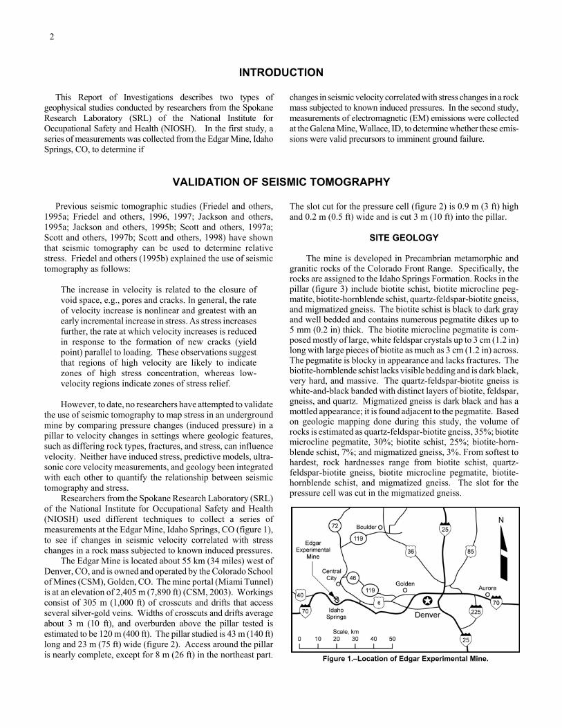
Researchers from the Spokane Research Laboratory (SRL) of the National Institute for Occupational Safety and Health (NIOSH) used different techniques to collect a series of measurements at the Edgar Mine, Idaho Springs, CO (figure 1), to see if changes in seismic velocity correlated with stress changes in a rock mass subjected to known induced pressures.
Figure 1.–Location of Edgar Experimental Mine.
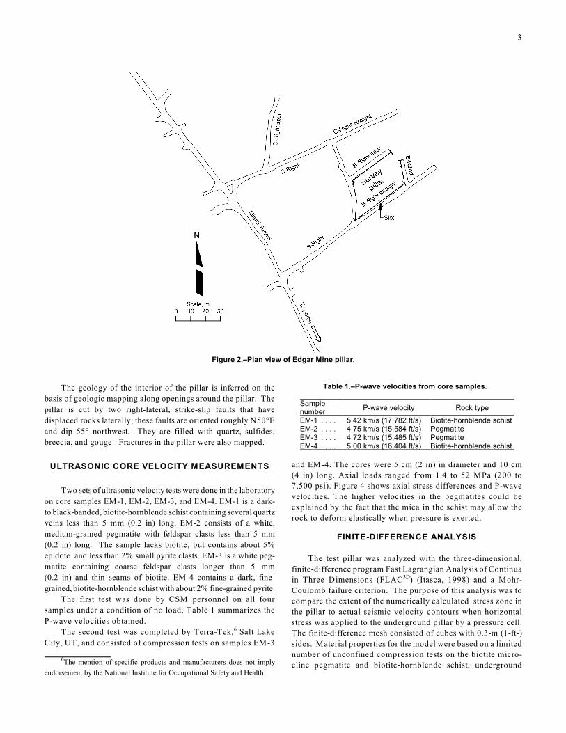
The Edgar Mine is located about 55 km (34 miles) west of Denver, CO, and is owned and operated by the Colorado School of Mines (CSM), Golden, CO. The mine portal (Miami Tunnel) is at an elevation of 2,405 m (7,890 ft) (CSM, 2003). Workings consist of 305 m (1,000 ft) of crosscuts and drifts that access several silver-gold veins. Widths of crosscuts and drifts average about 3 m (10 ft), and overburden above the pillar tested is estimated to be 120 m (400 ft). The pillar studied is 43 m (140 ft) long and 23 m (75 ft) wide (figure 2). Access around the pillar is nearly complete, except for 8 m (26 ft) in the northeast part.
The slot cut for the pressure cell (figure 2) is 0.9 m (3 ft) high and 0.2 m (0.5 ft) wide and is cut 3 m (10 ft) into the pillar.
SITE GEOLOGY
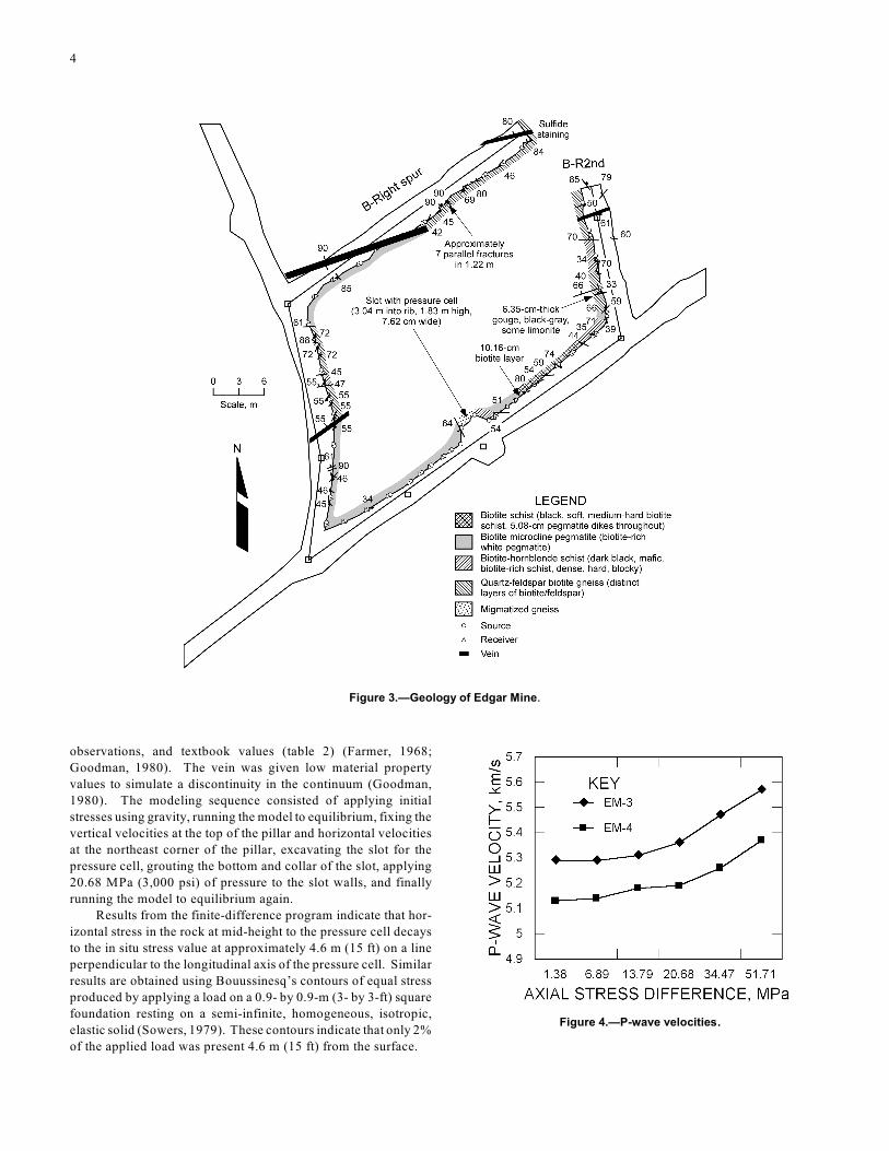
The mine is developed in Precambrian metamorphic and granitic rocks of the Colorado Front Range. Specifically, the rocks are assigned to the Idaho Springs Formation. Rocks in the pillar (figure 3) include biotite schist, biotite microcline peg-matite, biotite-hornblende schist, quartz-feldspar-biotite gneiss, and migmatized gneiss. The biotite schist is black to dark gray and well bedded and contains numerous pegmatite dikes up to 5 mm (0.2 in) thick. The biotite microcline pegmatite is com-posed mostly of large, white feldspar crystals up to 3 cm (1.2 in) long with large pieces of biotite as much as 3 cm (1.2 in) across. The pegmatite is blocky in appearance and lacks fractures. The biotite-hornblende schist lacks visible bedding and is dark black, very hard, and massive. The quartz-feldspar-biotite gneiss is white-and-black banded with distinct layers of biotite, feldspar, gneiss, and quartz. Migmatized gneiss is dark black and has a mottled appearance; it is found adjacent to the pegmatite. Based on geologic mapping done during this study, the volume of rocks is estimated as quartz-feldspar-biotite gneiss, 35%; biotite microcline pegmatite, 30%; biotite schist, 25%; biotite-horn-blende schist, 7%; and migmatized gneiss, 3%. From softest to hardest, rock hardnesses range from biotite schist, quartz-feldspar-biotite gneiss, biotite microcline pegmatite, biotite-hornblende schist, and migmatized gneiss. The slot for the pressure cell was cut in the migmatized gneiss.
3
Figure 2.–Plan view of Edgar Mine pillar.
The geology of the interior of the pillar is inferred on the
basis of geologic mapping along openings around the pillar. The
pillar is cut by two right-lateral, strike-slip faults that have
displaced rocks laterally; these faults are oriented roughly N50°E
and dip 55° northwest. They are filled with quartz, sulfides,
breccia, and gouge. Fractures in the pillar were also mapped.
ULTRASONIC CORE VELOCITY MEASUREMENTS
Two sets of ultrasonic velocity tests were done in the laboratory
on core samples EM-1, EM-2, EM-3, and EM-4. EM-1 is a dark-
to black-banded, biotite-hornblende schist containing several quartz
veins less than 5 mm (0.2 in) long. EM-2 consists of a white,
medium-grained pegmatite with feldspar clasts less than 5 mm
(0.2 in) long. The sample lacks biotite, but contains about 5%
epidote and less than 2% small pyrite clasts. EM-3 is a white peg
matite containing coarse feldspar clasts longer than 5 mm
(0.2 in) and thin seams of biotite. EM-4 contains a dark, fine-
grained, biotite-hornblende schist with about 2% fine-grained pyrite.
The first test was done by CSM personnel on all four
samples under a condition of no load. Table 1 summarizes the
P-wave velocities obtained.
Table 1.–P-wave velocities from core samples.
Sample number
P-wave velocity Rock type
EM-1 EM-2 EM-3 EM-4
. . . .
. . . .
. . . .
. . . .
5.42 km/s (17,782 ft/s) 4.75 km/s (15,584 ft/s) 4.72 km/s (15,485 ft/s) 5.00 km/s (16,404 ft/s)
Biotite-hornblende schist Pegmatite Pegmatite Biotite-hornblende schist
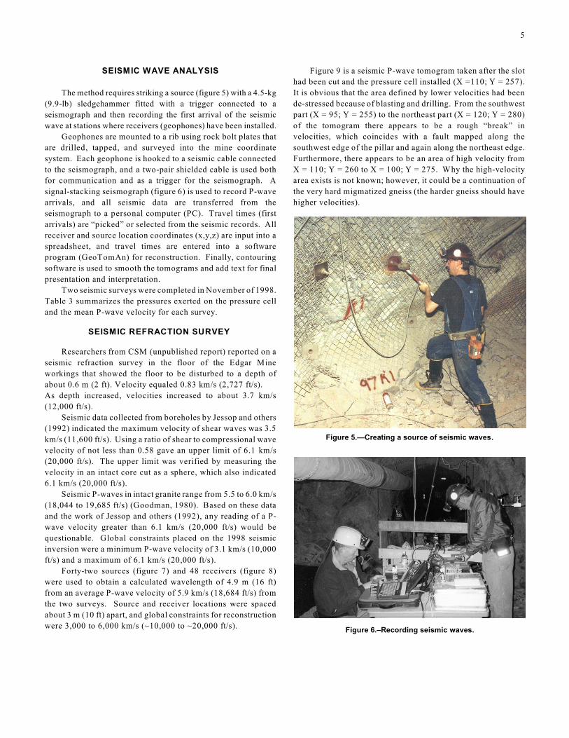
The second test was completed by Terra-Tek,6
6The mention of specific products and manufacturers does not imply
endorsement by the National Institute for Occupational Safety and Health.
Salt Lake
City, UT, and consisted of compression tests on samples EM-3
and EM-4. The cores were 5 cm (2 in) in diameter and 10 cm
(4 in) long. Axial loads ranged from 1.4 to 52 MPa (200 to
7,500 psi). Figure 4 shows axial stress differences and P-wave
velocities. The higher velocities in the pegmatites could be
explained by the fact that the mica in the schist may allow the
rock to deform elastically when pressure is exerted.
FINITE-DIFFERENCE ANALYSIS
The test pillar was analyzed with the three-dimensional,
finite-difference program Fast Lagrangian Analysis of Continua
in Three Dimensions (FLAC3D) (Itasca, 1998) and a Mohr-
Coulomb failure criterion. The purpose of this analysis was to
compare the extent of the numerically calculated stress zone in
the pillar to actual seismic velocity contours when horizontal
stress was applied to the underground pillar by a pressure cell.
The finite-difference mesh consisted of cubes with 0.3-m (1-ft-)
sides. Material properties for the model were based on a limited
number of unconfined compression tests on the biotite micro-
cline pegmatite and biotite-hornblende schist, underground
4
observations, and textbook values (table 2) (Farmer, 1968;
Goodman, 1980). The vein was given low material property
values to simulate a discontinuity in the continuum (Goodman,
1980). The modeling sequence consisted of applying initial
stresses using gravity, running the model to equilibrium, fixing the
vertical velocities at the top of the pillar and horizontal velocities
at the northeast corner of the pillar, excavating the slot for the
pressure cell, grouting the bottom and collar of the slot, applying
20.68 MPa (3,000 psi) of pressure to the slot walls, and finally
running the model to equilibrium again.
Figure 3.—Geology of Edgar Mine.
Figure 4.—P-wave velocities.
Results from the finite-difference program indicate that hor
izontal stress in the rock at mid-height to the pressure cell decays
to the in situ stress value at approximately 4.6 m (15 ft) on a line
perpendicular to the longitudinal axis of the pressure cell. Similar
results are obtained using Bouussinesq’s contours of equal stress
produced by applying a load on a 0.9- by 0.9-m (3- by 3-ft) square
foundation resting on a semi-infinite, homogeneous, isotropic,
elastic solid (Sowers, 1979). These contours indicate that only 2%
of the applied load was present 4.6 m (15 ft) from the surface.
5
SEISMIC WAVE ANALYSIS
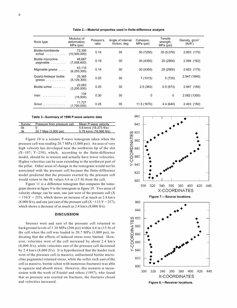
The method requires striking a source (figure 5) with a 4.5-kg
(9.9-lb) sledgehammer fitted with a trigger connected to a
seismograph and then recording the first arrival of the seismic
wave at stations where receivers (geophones) have been installed.
Figure 5.—Creating a source of seismic waves.
Geophones are mounted to a rib using rock bolt plates that
are drilled, tapped, and surveyed into the mine coordinate
system. Each geophone is hooked to a seismic cable connected
to the seismograph, and a two-pair shielded cable is used both
for communication and as a trigger for the seismograph. A
signal-stacking seismograph (figure 6) is used to record P-wave
arrivals, and all seismic data are transferred from the
seismograph to a personal computer (PC).
Figure 6.–Recording seismic waves.
Travel times (first
arrivals) are “picked” or selected from the seismic records. All
receiver and source location coordinates (x,y,z) are input into a
spreadsheet, and travel times are entered into a software
program (GeoTomAn) for reconstruction. Finally, contouring
software is used to smooth the tomograms and add text for final
presentation and interpretation.
Two seismic surveys were completed in November of 1998.
Table 3 summarizes the pressures exerted on the pressure cell
and the mean P-wave velocity for each survey.
SEISMIC REFRACTION SURVEY
Researchers from CSM (unpublished report) reported on a
seismic refraction survey in the floor of the Edgar Mine
workings that showed the floor to be disturbed to a depth of
about 0.6 m (2 ft). Velocity equaled 0.83 km/s (2,727 ft/s).
As depth increased, velocities increased to about 3.7 km/s
(12,000 ft/s).
Seismic data collected from boreholes by Jessop and others
(1992) indicated the maximum velocity of shear waves was 3.5
km/s (11,600 ft/s). Using a ratio of shear to compressional wave
velocity of not less than 0.58 gave an upper limit of 6.1 km/s
(20,000 ft/s). The upper limit was verified by measuring the
velocity in an intact core cut as a sphere, which also indicated
6.1 km/s (20,000 ft/s).
Seismic P-waves in intact granite range from 5.5 to 6.0 km/s
(18,044 to 19,685 ft/s) (Goodman, 1980). Based on these data
and the work of Jessop and others (1992), any reading of a P-
wave velocity greater than 6.1 km/s (20,000 ft/s) would be
questionable. Global constraints placed on the 1998 seismic
inversion were a minimum P-wave velocity of 3.1 km/s (10,000
ft/s) and a maximum of 6.1 km/s (20,000 ft/s).
Forty-two sources (figure 7) and 48 receivers (figure 8)
were used to obtain a calculated wavelength of 4.9 m (16 ft)
from an average P-wave velocity of 5.9 km/s (18,684 ft/s) from
the two surveys. Source and receiver locations were spaced
about 3 m (10 ft) apart, and global constraints for reconstruction
were 3,000 to 6,000 km/s (~10,000 to ~20,000 ft/s).
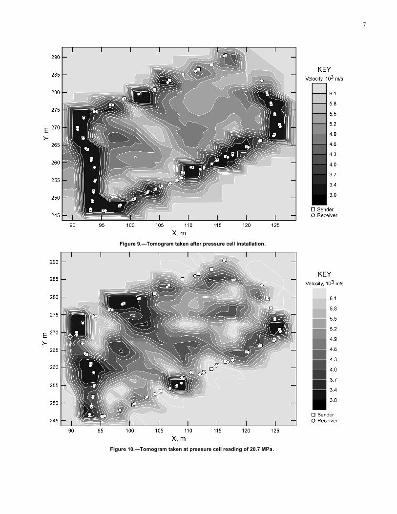
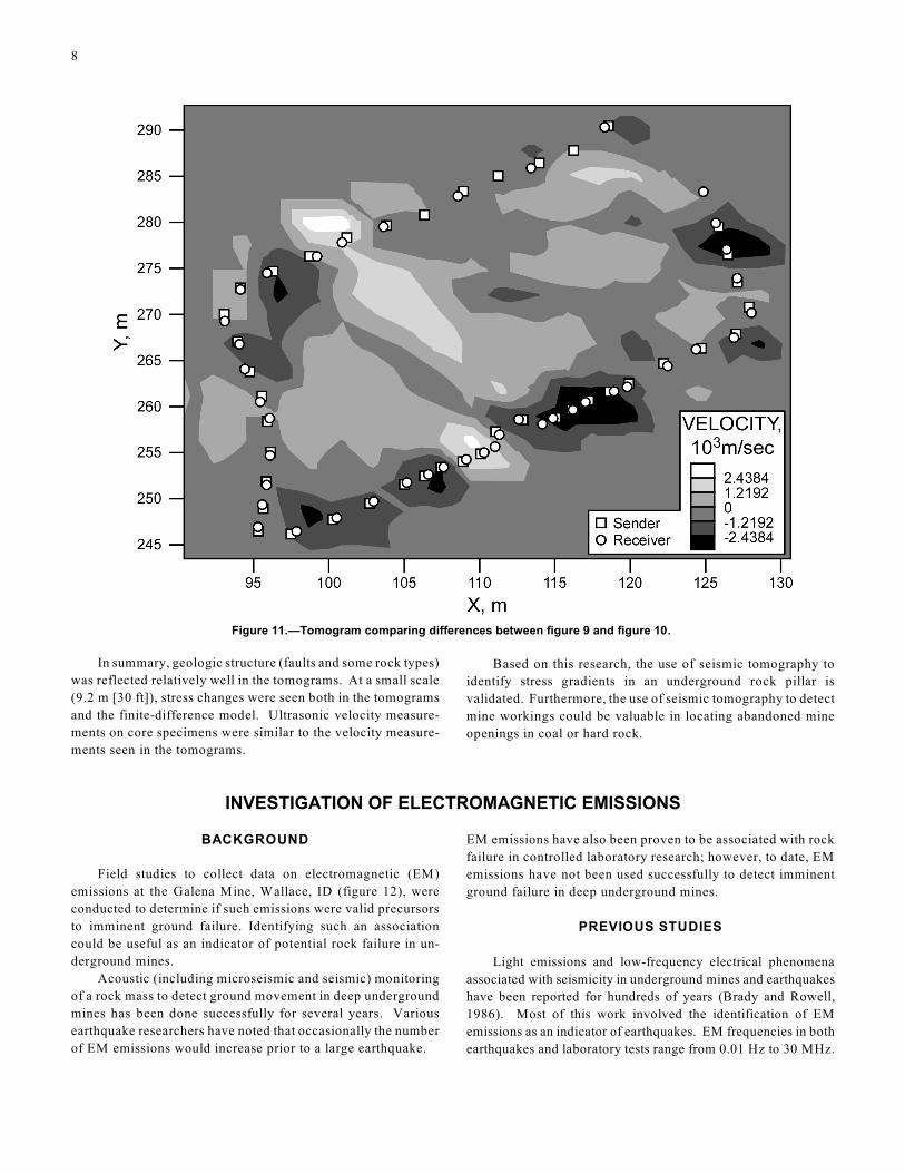
Figure 9 is a seismic P-wave tomogram taken after the slot
had been cut and the pressure cell installed (X =110; Y = 257).
It is obvious that the area defined by lower velocities had been
de-stressed because of blasting and drilling. From the southwest
part (X = 95; Y = 255) to the northeast part (X = 120; Y = 280)
of the tomogram there appears to be a rough “break” in
velocities, which coincides with a fault mapped along the
southwest edge of the pillar and again along the northeast edge.
Furthermore, there appears to be an area of high velocity from
X = 110; Y = 260 to X = 100; Y = 275. Why the high-velocity
area exists is not known; however, it could be a continuation of
the very hard migmatized gneiss (the harder gneiss should have
higher velocities).
6
Table 2.—Material properties used in finite-difference analysis
Rock type Modulus of
deformation, MPa (psi)
Poisson’s ratio
Angle of internalfriction, deg
Cohesion, MPa (psi)
Tensile strength,MPa (psi)
Density, g/cm3
(lb/ft )3
Biotite-hornblende schist . . . . . . . . . . .
72,395 (10,500,000)
0.14 35 50 (7250) 35 (5,076) 2.803 (175)
Biotite microcline pegmatite . . . . . . . .
48,667 (7,058,600)
0.19 30 30 (4350) 20 (2900) 2.594 (162)
Migmatite gneiss . . . . 43,115
(6,253,300) 0.14 30 30 (4350) 20 (2900) 2.803 (175)
Quartz-feldspar biotitegneiss . . . . . . . . . . .
35,365 (5,129,300)
0.25 30 7 (1015) 5 (725) 2.947 (1840)
Biotite schist . . . . . . . 22,063
(3,200,000) 0.25 30 2.5 (363) 0.5 (973) 2.947 (184)
Vein . . . . . . . . . . . . . 134
(19,500) 0.30 30 0 0 2.082 (1300)
Grout . . . . . . . . . . . . . 11,721
(1,700,000) 0.25 35 11.5 (1670) 4.4 (640) 2.403 (150)
Table 3.–Summary of 1998 P-wave seismic data
Survey Pressure from pressure cell Mean P-wave velocity 0k 0 5.6 km/s (18,373 ft/s) 3k 20.7 Mpa (3,000 psi) 5.79 km/s (18,996 ft/s)
Figure 7.—Source locations.
Figure 8.—Receiver locations.
Figure 10 is a seismic P-wave tomogram taken when the
pressure cell was reading 20.7 MPa (3,000 psi). An area of very
high velocity has developed near the northwest tip of the slot
(X~107; Y~258), which, according to the finite-difference
model, should be in tension and actually have lower velocities.
Higher velocities can be seen extending to the northwest part of
the pillar. Other areas of change in the tomogram would not be
associated with the pressure cell because the finite-difference
model predicted that the pressure exerted by the pressure cell
would return to the 0k values 4.6 m (15 ft) from the cell.
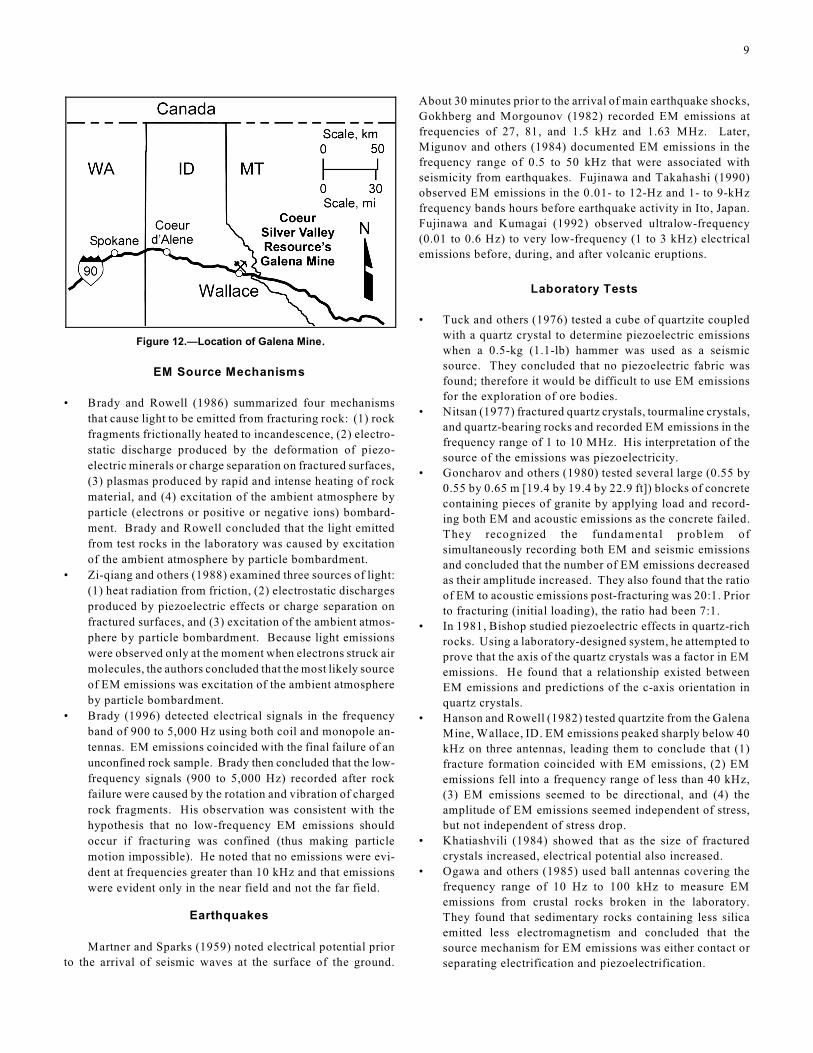
Figure 11 is a difference tomogram that compares the tomo
gram shown in figure 9 to the tomogram in figure 10. Two areas of
velocity change can be seen, one just west of the pressure cell (X
= 110;Y = 255), which shows an increase of as much as 2.4 km/s
(8,000 ft/s), and one just east of the pressure cell (X =115;Y = 257),
which shows a decrease of as much as 2.4 km/s (8,000 ft/s).
DISCUSSION
Stresses west and east of the pressure cell returned to
background levels of 1.38 MPa (200 psi) within 4.6 m (15 ft) of
the cell when the cell was loaded to 20.7 MPa (3,000 psi), in
dicating that the effects of induced stress were limited. How
ever, velocities west of the cell increased by about 2.4 km/s
(8,000 ft/s), while velocities east of the pressure cell decreased
by 2.4 km/s (8,000 ft/s). It is hypothesized that the harder rock
west of the pressure cell (a massive, unfractured biotite micro-
cline pegmatite) retained stress, while the softer rock east of the
cell (a massive, biotite schist with numerous fractures) was able
to squeeze and absorb stress. However, this scenario is incon
sistent with the work of Friedel and others (1997), who found
that as pressure was exerted on fractures, the fractures closed
and velocities increased.
7
Figure 9.—Tomogram taken after pressure cell installation.
Figure 10.—Tomogram taken at pressure cell reading of 20.7 MPa.
8
Figure 11.—Tomogram comparing differences between figure 9 and figure 10.
In summary, geologic structure (faults and some rock types)
was reflected relatively well in the tomograms. At a small scale
(9.2 m [30 ft]), stress changes were seen both in the tomograms
and the finite-difference model. Ultrasonic velocity measure-
ments on core specimens were similar to the velocity measure-
ments seen in the tomograms.
Based on this research, the use of seismic tomography to
identify stress gradients in an underground rock pillar is
validated. Furthermore, the use of seismic tomography to detect
mine workings could be valuable in locating abandoned mine
openings in coal or hard rock.
INVESTIGATION OF ELECTROMAGNETIC EMISSIONS
BACKGROUND
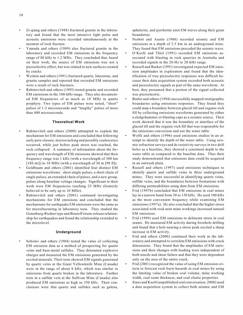
Field studies to collect data on electromagnetic (EM)
emissions at the Galena Mine, Wallace, ID (figure 12), were
conducted to determine if such emissions were valid precursors
to imminent ground failure. Identifying such an association
could be useful as an indicator of potential rock failure in un
derground mines.
Acoustic (including microseismic and seismic) monitoring
of a rock mass to detect ground movement in deep underground
mines has been done successfully for several years. Various
earthquake researchers have noted that occasionally the number
of EM emissions would increase prior to a large earthquake.
EM emissions have also been proven to be associated with rock
failure in controlled laboratory research; however, to date, EM
emissions have not been used successfully to detect imminent
ground failure in deep underground mines.
PREVIOUS STUDIES
Light emissions and low-frequency electrical phenomena
associated with seismicity in underground mines and earthquakes
have been reported for hundreds of years (Brady and Rowell,
1986). Most of this work involved the identification of EM
emissions as an indicator of earthquakes. EM frequencies in both
earthquakes and laboratory tests range from 0.01 Hz to 30 MHz.
9
Figure 12.—Location of Galena Mine.
EM Source Mechanisms
• Brady and Rowell (1986) summarized four mechanisms
that cause light to be emitted from fracturing rock: (1) rock
fragments frictionally heated to incandescence, (2) electro
static discharge produced by the deformation of piezo
electric minerals or charge separation on fractured surfaces,
(3) plasmas produced by rapid and intense heating of rock
material, and (4) excitation of the ambient atmosphere by
particle (electrons or positive or negative ions) bombard
ment. Brady and Rowell concluded that the light emitted
from test rocks in the laboratory was caused by excitation
of the ambient atmosphere by particle bombardment.
• Zi-qiang and others (1988) examined three sources of light:
(1) heat radiation from friction, (2) electrostatic discharges
produced by piezoelectric effects or charge separation on
fractured surfaces, and (3) excitation of the ambient atmos
phere by particle bombardment. Because light emissions
were observed only at the moment when electrons struck air
molecules, the authors concluded that the most likely source
of EM emissions was excitation of the ambient atmosphere
by particle bombardment.
• Brady (1996) detected electrical signals in the frequency
band of 900 to 5,000 Hz using both coil and monopole an
tennas. EM emissions coincided with the final failure of an
unconfined rock sample. Brady then concluded that the low-
frequency signals (900 to 5,000 Hz) recorded after rock
failure were caused by the rotation and vibration of charged
rock fragments. His observation was consistent with the
hypothesis that no low-frequency EM emissions should
occur if fracturing was confined (thus making particle
motion impossible). He noted that no emissions were evi
dent at frequencies greater than 10 kHz and that emissions
were evident only in the near field and not the far field.
Earthquakes
Martner and Sparks (1959) noted electrical potential prior
to the arrival of seismic waves at the surface of the ground.
About 30 minutes prior to the arrival of main earthquake shocks,
Gokhberg and Morgounov (1982) recorded EM emissions at
frequencies of 27, 81, and 1.5 kHz and 1.63 MHz. Later,
Migunov and others (1984) documented EM emissions in the
frequency range of 0.5 to 50 kHz that were associated with
seismicity from earthquakes. Fujinawa and Takahashi (1990)
observed EM emissions in the 0.01- to 12-Hz and 1- to 9-kHz
frequency bands hours before earthquake activity in Ito, Japan.
Fujinawa and Kumagai (1992) observed ultralow-frequency
(0.01 to 0.6 Hz) to very low-frequency (1 to 3 kHz) electrical
emissions before, during, and after volcanic eruptions.
Laboratory Tests
• Tuck and others (1976) tested a cube of quartzite coupled
with a quartz crystal to determine piezoelectric emissions
when a 0.5-kg (1.1-lb) hammer was used as a seismic
source. They concluded that no piezoelectric fabric was
found; therefore it would be difficult to use EM emissions
for the exploration of ore bodies.
• Nitsan (1977) fractured quartz crystals, tourmaline crystals,
and quartz-bearing rocks and recorded EM emissions in the
frequency range of 1 to 10 MHz. His interpretation of the
source of the emissions was piezoelectricity.
• Goncharov and others (1980) tested several large (0.55 by
0.55 by 0.65 m [19.4 by 19.4 by 22.9 ft]) blocks of concrete
containing pieces of granite by applying load and record
ing both EM and acoustic emissions as the concrete failed.
They recognized the fundamental problem of
simultaneously recording both EM and seismic emissions
and concluded that the number of EM emissions decreased
as their amplitude increased. They also found that the ratio
of EM to acoustic emissions post-fracturing was 20:1. Prior
to fracturing (initial loading), the ratio had been 7:1.
• In 1981, Bishop studied piezoelectric effects in quartz-rich
rocks. Using a laboratory-designed system, he attempted to
prove that the axis of the quartz crystals was a factor in EM
emissions. He found that a relationship existed between
EM emissions and predictions of the c-axis orientation in
quartz crystals.
• Hanson and Rowell (1982) tested quartzite from the Galena
Mine, Wallace, ID. EM emissions peaked sharply below 40
kHz on three antennas, leading them to conclude that (1)
fracture formation coincided with EM emissions, (2) EM
emissions fell into a frequency range of less than 40 kHz,
(3) EM emissions seemed to be directional, and (4) the
amplitude of EM emissions seemed independent of stress,
but not independent of stress drop.
• Khatiashvili (1984) showed that as the size of fractured
crystals increased, electrical potential also increased.
• Ogawa and others (1985) used ball antennas covering the
frequency range of 10 Hz to 100 kHz to measure EM
emissions from crustal rocks broken in the laboratory.
They found that sedimentary rocks containing less silica
emitted less electromagnetism and concluded that the
source mechanism for EM emissions was either contact or
separating electrification and piezoelectrification.
10
• Zi-qiang and others (1988) fractured granite in the labora
tory and found that the most intensive light pulse and
acoustic emissions were recorded simultaneously at the
moment of rock fracture.
• Yamada and others (1989) also fractured granite in the
laboratory and recorded EM emissions in the frequency
range of 80 kHz to 1.2 MHz. They concluded that, based
on their work, the source of EM emissions was not a
piezoelectric effect, but was related to new surfaces created
by cracks.
• Weimin and others (1991) fractured quartz, limestone, and
granite samples and reported that recorded EM emissions
were a result of rock fractures.
• Rabinovitch and others (1995) tested granite and recorded
EM emissions in the 100-kHz range. They also document
ed EM frequencies of as much as 10 MHz in quartz
porphyry. Two types of EM pulses were noted, “short”
pulses of 1-3 microseconds and “lengthy” pulses of more
than 400 microseconds.
Theoretical Work
• Rabinovitch and others (2000) attempted to explain the
mechanism for EM emissions and concluded that following
early pore closure, microcracking and possibly coalescence
occurred, while just before peak stress was reached, the
rock collapsed. A summary of information about the fre
quency and wavelength of EM emissions showed that their
frequency range was 1 kHz (with a wavelength of 300 km
[186 mi]) to 10 MHz (with a wavelength of 30 m [98 ft]).
• Goldbaum and others (2001) identified four distinct EM
emissions waveforms: short single pulses, a short chain of
single pulses, an extended chain of pulses, and a new group,
pulses along baseline voltage changes. Significant to their
work were EM frequencies reaching 25 MHz (formerly
believed to be only up to 10 MHz).
• Rabinovitch and others (2001) continued investigating
mechanisms for EM emissions and concluded that the
mechanisms for earthquake EM emissions were the same as
for microfracturing in laboratory tests. They studied the
Gutenburg-Richter type and Benioff strain-release relation
ship for earthquakes and found the relationship extended to
the microlevel.
Underground
• Sobolev and others (1984) tested the value of collecting
EM emission data as a method of prospecting for quartz
veins and base-metal sulfides. They detonated explosive
charges and measured the EM emissions generated by the
excited minerals. Their tests showed EM signals generated
by quartz veins at the Giant Yellowknife Mine (Canada)
were in the range of about 8 kHz, which was similar to
emissions from quartz broken in the laboratory. Further
tests in a sulfide vein at the Sullivan Mine (Canada) also
produced EM emissions as high as 350 kHz. Their con
clusions were that quartz and sulfides such as galena,
sphalerite, and pyrrhotite emit EM waves along their grain
boundaries.
• Nesbitt and Austin (1988) recorded seismic and EM
emissions at a depth of 2.5 km in an underground mine.
They found that EM emissions preceded the seismic wave.
• O’Keefe and Thiel (1991) recorded EM emissions as
sociated with blasting in rock quarries in Australia and
recorded signals in the 20-Hz to 20-kHz range.
• Russell and Barker (1991) investigated expected EM emis
sion amplitudes in exploration and found that the iden
tification of true piezoelectric responses was difficult be
cause their data acquisition system recorded both acoustic
and piezoelectric signals as part of the same waveform. At
best, they presumed that a portion of the signal collected
was piezoelectric.
• Butler and others (1994) successfully mapped stratigraphic
boundaries using emissions responses. They found they
could map a boundary between glacial till and organic-rich
fill by collecting emissions waveforms generated by either
a sledgehammer or blasting caps as a seismic source. Their
work showed that it was the boundary or interface of the
glacial till and the organic-rich fill that was responsible for
the emissions conversion and not the water table.
• Wolfe and others (1996) used emissions studies in an at
tempt to identify the depth of the water table. Using seis
mic refraction surveys and dc resistivity surveys in two drill
holes as a baseline, they showed a consistent depth to the
water table as compared to the baseline data. Thus their
study demonstrated that emissions data could be acquired
in an outwash plain.
• Russell and others (1997) used emissions techniques to
identify quartz and sulfide veins in three underground
mines. They were successful in identifying quartz veins,
sulfide veins, and the boundaries between formations with
differing permeabilities using data from EM emissions.
• Frid (1997b) concluded that EM emissions in coal mines
lay in a narrow band from 30 to 150 kHz. He used 100 kHz
as the most convenient frequency while examining EM
emissions (1997a). He also concluded that the higher stress
associated with rock near mine workings increased natural
EM emissions.
• Frid (1999) used EM emissions to delineate stress in coal
seams. He measured EM activity during borehole drilling
and found that a hole nearing a stress peak excited a sharp
increase in EM activity.
• Frid and others (2000) continued their work in the lab
oratory and attempted to correlate EM emissions with crack
dimensions. They found that the amplitudes of EM emis
sions and their changes with loading were independent of
both tensile and shear failure and that they were dependent
only on the area of the entire crack.
• Frid (2001) recognized the value of using EM emission cri
teria to forecast rock burst hazards in coal mines by using
the limiting value of broken coal volume, mine working
width, coal seam thickness, and coal elastic properties.
• Sines and Knoll (unpublished oral conversation, 2000) used
a data acquisition system to collect both seismic and EM
11
emissions on the 4600 level of the Galena Mine. They
sampled at a rate of about 7,200 samples per second (a
Nyquist frequency of 3,500 Hz) using two monopole
antennas 12.5 and 15.2 m (41 and 49.9 ft) long. They used
no filters to eliminate low-frequency emissions and found
numerous triggers on the EM antenna, which were initially
thought to be coincident with seismic activity. However,
when the EM and seismic waveforms were analyzed, they
found that most of the seismic emissions had actually
preceded the EM emissions, which is physically impossible.
Further evaluation of the collected waveforms showed that
most of the EM emissions were caused by mine cultural
noise, which included the opening and closing of air doors
(60-Hz solenoid), locomotive activity, and chute loading.
• Butler and others (2001) conducted field studies at the
Brunswick No. 12 Mine in Canada in an attempt to link EM
emissions with seismic activity and also to delineate sulfide
ore. They used various antennas covering a range of
frequencies from 1 Hz to 4.5 MHz. They found that
broadband EM emissions with frequencies up to 800 kHz
could be induced by seismicity and blasting. However,
results did not confirm that EM emissions preceded
seismicity.
• Vozoff (2002) attempted to demonstrate the use of EM
monitoring as a warning system for roof failure in a large
coal seam in Australia. He collected three complete data
sets and concluded that of the three, one set coincided with
a roof fall and was correlated with EM activity, one set
might have had a “weak correlation at best,” and one set
had no EM correlations with roof falls.
TECHNICAL APPROACH
As noted above, many researchers have attempted to
capture EM emissions before, during, or after ground failure
(i.e., rock bursts) in underground mines. However, to date, none
have conclusively linked rock breaking underground with EM
emissions. The following work describes the methods and re
sults of a study at the Galena Mine, Wallace, ID. It builds on
the work of previous researchers, but uses new methods in an
attempt to capture EM emissions from either blasting or rock
bursting.
The equipment used included an ESG data acquisition
system, ULTRAQ, capable of sampling up to 10 million samples
per second (Nyquist frequency of 5 million samples per second)
on four channels and a Pentium 166 computer. The system was
enclosed in a box to keep it as clean and dry as possible; fans
were installed to keep air moving in the box. Voltages for
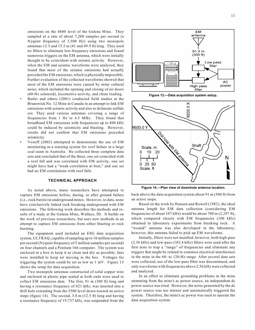
triggering the system could be set as low as 1 mV. Figure 13
shows the setup for data acquisition.
Figure 13.—Data acquisition system setup.
Two monopole antennas constructed of solid copper wire
and enclosed in plastic pipe sealed at both ends were used to
collect EM emissions data. The first, 91 m (300 ft) long and
having a resonance frequency of 821 kHz, was inserted into a
drill hole extending from the 5500 level down toward an active
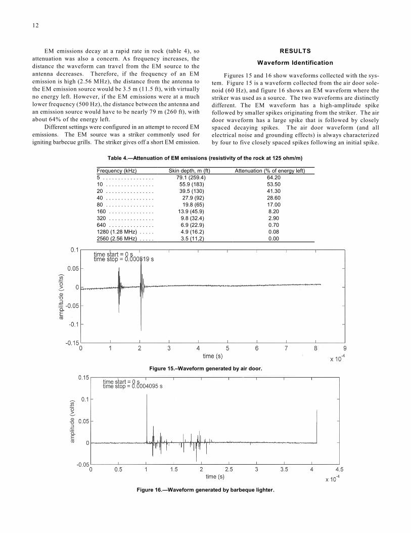
stope (figure 14).
Figure 14.—Plan view of downhole antenna location.
The second, 3.8 m (12.5 ft) long and having
a resonance frequency of 19,737 kHz, was suspended from the
back above the data acquisition system about 91 m (300 ft) from
an active stope.
Based on the work by Hanson and Rowell (1982), the ideal
antenna length for EM data collection (considering EM
frequencies of about 107 kHz) would be about 700 m (2,297 ft),
which compared closely with EM frequencies (100 kHz)
obtained in laboratory experiments from breaking rock. A
“wound” antenna was also developed in the laboratory;
however, this antenna failed to pick up EM waveforms.
Initially, filters were not installed; however, both high-pass
(2.56 kHz) and low-pass (102.4 kHz) filters were used after the
first tests to trap a “range” of frequencies and eliminate any
triggers that might be related to common electrical interference
in the mine in the 60- to 120-Hz range. After several data sets
were collected, use of the low-pass filter was discontinued, and
only waveforms with frequencies above 2.56 kHz were collected
and analyzed.
In an effort to eliminate grounding problems in the mine
stemming from the mine's ac power source, an independent dc
power source was tried. However, the noise generated by the dc
power source was too intense and automatically triggered the
system. Therefore, the mine's ac power was used to operate the
data acquisition system.
12
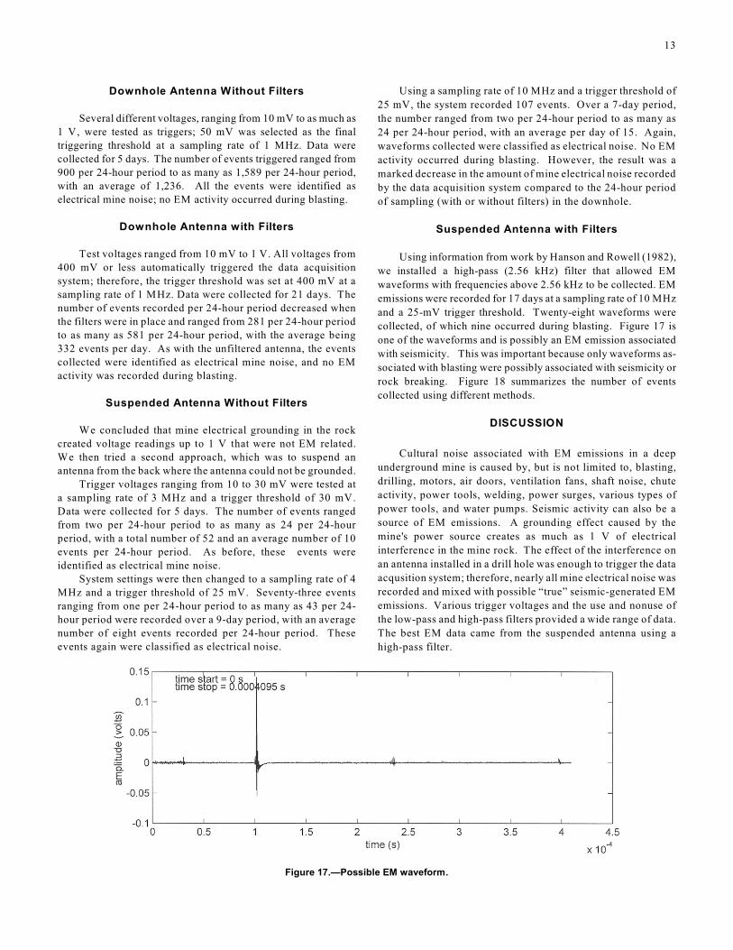
EM emissions decay at a rapid rate in rock (table 4), so
attenuation was also a concern.
Table 4.—Attenuation of EM emissions (resistivity of the rock at 125 ohm/m)
Frequency (kHz) Skin depth, m (ft) Attenuation (% of energy left)
5 . . . . . . . . . . . . . . . . . 79.1 (259.4) 64.20
10 . . . . . . . . . . . . . . . . 55.9 (183) 53.50
20 . . . . . . . . . . . . . . . . 39.5 (130) 41.30
40 . . . . . . . . . . . . . . . . 27.9 (92) 28.60
80 . . . . . . . . . . . . . . . . 19.8 (65) 17.00
160 . . . . . . . . . . . . . . . 13.9 (45.9) 8.20
320 . . . . . . . . . . . . . . . 9.8 (32.4) 2.90
640 . . . . . . . . . . . . . . . 6.9 (22.9) 0.70
1280 (1.28 MHz) . . . . . 4.9 (16.2) 0.08
2560 (2.56 MHz) . . . . . 3.5 (11,2) 0.00
As frequency increases, the
distance the waveform can travel from the EM source to the
antenna decreases. Therefore, if the frequency of an EM
emission is high (2.56 MHz), the distance from the antenna to
the EM emission source would be 3.5 m (11.5 ft), with virtually
no energy left. However, if the EM emissions were at a much
lower frequency (500 Hz), the distance between the antenna and
an emission source would have to be nearly 79 m (260 ft), with
about 64% of the energy left.
Different settings were configured in an attempt to record EM
emissions. The EM source was a striker commonly used for
igniting barbecue grills. The striker gives off a short EM emission.
RESULTS
Waveform Identification
Figures 15 and 16 show waveforms collected with the system. Figure 15 is a waveform collected from the air door solenoid (60 Hz), and figure 16 shows an EM waveform where the striker was used as a source.
Figure 15.–Waveform generated by air door.
Figure 16.—Waveform generated by barbeque lighter.
The two waveforms are distinctly different. The EM waveform has a high-amplitude spike followed by smaller spikes originating from the striker. The air door waveform has a large spike that is followed by closely spaced decaying spikes. The air door waveform (and all electrical noise and grounding effects) is always characterized by four to five closely spaced spikes following an initial spike.
13
Downhole Antenna Without Filters
Several different voltages, ranging from 10 mV to as much as
1 V, were tested as triggers; 50 mV was selected as the final
triggering threshold at a sampling rate of 1 MHz. Data were
collected for 5 days. The number of events triggered ranged from
900 per 24-hour period to as many as 1,589 per 24-hour period,
with an average of 1,236. All the events were identified as
electrical mine noise; no EM activity occurred during blasting.
Downhole Antenna with Filters
Test voltages ranged from 10 mV to 1 V. All voltages from
400 mV or less automatically triggered the data acquisition
system; therefore, the trigger threshold was set at 400 mV at a
sampling rate of 1 MHz. Data were collected for 21 days. The
number of events recorded per 24-hour period decreased when
the filters were in place and ranged from 281 per 24-hour period
to as many as 581 per 24-hour period, with the average being
332 events per day. As with the unfiltered antenna, the events
collected were identified as electrical mine noise, and no EM
activity was recorded during blasting.
Suspended Antenna Without Filters
We concluded that mine electrical grounding in the rock
created voltage readings up to 1 V that were not EM related.
We then tried a second approach, which was to suspend an
antenna from the back where the antenna could not be grounded.
Trigger voltages ranging from 10 to 30 mV were tested at
a sampling rate of 3 MHz and a trigger threshold of 30 mV.
Data were collected for 5 days. The number of events ranged
from two per 24-hour period to as many as 24 per 24-hour
period, with a total number of 52 and an average number of 10
events per 24-hour period. As before, these events were
identified as electrical mine noise.
System settings were then changed to a sampling rate of 4
MHz and a trigger threshold of 25 mV. Seventy-three events
ranging from one per 24-hour period to as many as 43 per 24
hour period were recorded over a 9-day period, with an average
number of eight events recorded per 24-hour period. These
events again were classified as electrical noise.
Using a sampling rate of 10 MHz and a trigger threshold of
25 mV, the system recorded 107 events. Over a 7-day period,
the number ranged from two per 24-hour period to as many as
24 per 24-hour period, with an average per day of 15. Again,
waveforms collected were classified as electrical noise. No EM
activity occurred during blasting. However, the result was a
marked decrease in the amount of mine electrical noise recorded
by the data acquisition system compared to the 24-hour period
of sampling (with or without filters) in the downhole.
Suspended Antenna with Filters
Using information from work by Hanson and Rowell (1982),
we installed a high-pass (2.56 kHz) filter that allowed EM
waveforms with frequencies above 2.56 kHz to be collected. EM
emissions were recorded for 17 days at a sampling rate of 10 MHz
and a 25-mV trigger threshold. Twenty-eight waveforms were
collected, of which nine occurred during blasting. Figure 17 is
one of the waveforms and is possibly an EM emission associated
with seismicity.
Figure 17.—Possible EM waveform.
This was important because only waveforms as
sociated with blasting were possibly associated with seismicity or
rock breaking. Figure 18 summarizes the number of events
collected using different methods.
DISCUSSION
Cultural noise associated with EM emissions in a deep
underground mine is caused by, but is not limited to, blasting,
drilling, motors, air doors, ventilation fans, shaft noise, chute
activity, power tools, welding, power surges, various types of
power tools, and water pumps. Seismic activity can also be a
source of EM emissions. A grounding effect caused by the
mine's power source creates as much as 1 V of electrical
interference in the mine rock. The effect of the interference on
an antenna installed in a drill hole was enough to trigger the data
acqusition system; therefore, nearly all mine electrical noise was
recorded and mixed with possible “true” seismic-generated EM
emissions. Various trigger voltages and the use and nonuse of
the low-pass and high-pass filters provided a wide range of data.
The best EM data came from the suspended antenna using a
high-pass filter.
14
Figure 18.–Summary of waveforms collected.
However, results to date suggest that (1) the number of EM
emissions prior to recorded seismic activity does not increase,
(2) some EM signals are generated during blasting, (3)
interference from mine electrical sources mask true EM signals,
(4) EM emissions do not give enough warning (compared to
seismic monitoring) to permit miners to leave a stope, (5) the
distance an EM signal can travel in the rock is between 18 and
40 m (58 and 130 ft), and (6) current data acquisition systems do
not differentiate between EM signals generated from seismic
activity and random mine electrical noise. In summary, these
results preclude monitoring EM emissions as precursors of
impending catastrophic ground failure.
CONCLUSIONS
This Report of Investigations describes two geophysical
methods examined by NIOSH researchers to identify and
characterize conditions that might lead to ground failure in
highly stressed rock in underground mines. Such studies are
important in that identification of precursors to rock failure
could lead to measures that could reduce or prevent injuries and
deaths among miners.
Key findings concerning the use of seismic tomography
were that (1) seismic tomograms showed that seismic velocities
in rock adjacent to mine openings were low, (2) a difference
tomogram in which in situ stresses on the east and west sides of
the slot were compared showed that velocities increased west of
the slot, but decreased east of the slot, (3) geologic features
(rock types and a fault) identified through geologic mapping
were recognizable in the seismic tomograms, (4) ultrasonic
velocity measurements on the rock cores agreed with seismic
velocity measurements in the tomograms, and (5) results from
the finite-difference analysis compared well to the seismic
tomograms west of the slot, but not east of the slot.
Results from studies of the use of EM emissions as
precursors to seismic activity indicated that (1) the number of
EM emissions does not increase prior to recorded seismic
activity, (2) some EM signals are generated during blasting,
(3) interference from mine electrical sources mask seismic-
generated EM signals, (4) EM emissions do not give enough
warning to permit miners to leave a stope, (5) the distance an
EM signal can travel in rock is between 18 and 40 m (58 and
130 ft), and (6) current data acquisition systems do not
differentiate between EM signals generated from seismic
activity and random mine electrical noise.
ACKNOWLEDGMENTS
The authors wish to thank Harry Cougher (general manager,
Galena Mine) for access to the Galena Mine. The authors also
wish to thank Mr. Bill Matthews of Golden Drilling, Canon
City, CO, for providing diamond drill experience during
installation of the pressure cell. CSM provided mine access,
utilities, geologic and mine maps, and engineering students who
mapped the coordinates for the geophone receiver locations.
Dr. Michael Friedel, USGS, Lakewood, CO, provided valuable
editing input for the final manuscript.
15
REFERENCES
Bishop, J.R. 1981. Piezoelectric Effects in Quartz-Rich Rocks. Tectonophysics, vol. 77, pp. 297-321.
Brady, B.T. 1992. Electrodynamics of Rock Fracture: Implications for Models of Rock Fracture. In Proceedings, Workshop on Low-Frequency Electrical Precursors, ed. by S.K. Park. Report 92-15, IGPP, Univ. of California-Riverside, 1992.
Brady, B.T., and G.A. Rowell. 1986. Laboratory Investigation of the Electrodynamics of Rock Failure. Nature, vol. 321, no. 6069, May 29, pp. 1-5.
Butler, K.E., R.D. Russell, A.W. Kepic, and M. Maxwell. 1994. Mapping of a Stratigraphic Boundary by its Seismo-electric Response. In Proceedings of the Symposium on the Application of Geophysics to Engineering and Environmental Problems, ed. by R.S. Bell and C.M. Lepper (Boston, MA, Mar. 27-31, 1994). Environ. and Eng. Geophys. Soc., vol. 2, pp. 689-699.
Butler, K.E., Bradford Simser, and Roger Bowes. 2001. An Experimental Field Trial of Passive Seismoelectric Monitoring. Canadian Geophysical Union, Ottawa, ON, Canada, May 14-17, 2001.
Colorado School of Mines. 2003. Idaho Springs Tunnel Detection Test Facility Constructed and Maintained for the U.S. Army Belvoir Research and Development Center by the Department of Mining Engineering, Colorado School of Mines. Brochure prepared by the Colorado School of Mines, 13 pp.
Farmer, I.W. 1968. Engineering Properties of Rock. Butler and Tanner, London, 180 pp.
Frid, V. 1997a. Rockburst Hazard Forecast by Electromagnetic Radiation Excited by Rock Fracture. Rock Mechanics Rock Engineering, vol. 30, No. 4, pp. 229-236.
Frid, V. 1997b. Electromagnetic Radiation Method for Rock and Gas Outburst Forecast. Journal of Applied Geophysics, vol. 38, pp. 97-104.
Frid, V. 2000. Electromagnetic Radiation Method Water-Infusion Control in Rockburst-Prone Strata. Journal of Applied Geophysics, vol. 43, 2000 , pp. 5-13.
Frid, V. 2001. Calculation of Electromagnetic Radiation Criterion for Rockburst Hazard Forecast in Coal Mines. Pure and Applied Geophysics, vol. 158, pp. 931-944.
Frid, V., D. Bahat, J. Goldbaum, and A. Rabinovitch. 2000. Experimental and Theoretical Investigations of Electromagnetic Radiation Induced by Rock Fracture. Israel Journal of Earth Science, vol. 49, pp. 9-19.
Friedel, M.J., M.J. Jackson, D.F. Scott, T.J. Williams, and M.S. Olson. 1995a. 3D Tomographic Imaging of Anomalous Conditions in a Deep Silver Mine. Applied Geophysics, vol. 34, pp. 1-21.
Friedel, M.J., D.F. Scott, M.J. Jackson, T.J. Williams, and S.M. Killen. 1995b. 3D Seismic Tomographic Imaging of Mechanical Conditions in a Deep U.S. Gold Mine. In Mechanics of Jointed and Faulted Rock-2. Proceedings of the International Conference on Mechanics o f Jointed and Faulted Rock (Tech. Univ. of Vienna, Vienna, Austria, April 13-17, 1995). Balkema, Rotterdam, pp. 689-695.
Friedel, M.J., D.F. Scott, M.J. Jackson, T.J. Williams, and S.M. Killen. 1996. 3D Seismic Tomographic Imaging of Anomalous Stress Conditions in a Deep U.S. Gold Mine. Applied Geophysics, vol. 36, pp. 1-17.
Friedel, M.J., D.F. Scott, and T.J. Williams. 1997. Temporal Imaging of Mine-Induced Stress Change Using Seismic Tomography. Engineering Geology, vol. 46, pp. 131-141.
Fujinawa, Y., and T. Kumagai. 1992. A Study of Anomalous Underground Electric Field Variations Associated with a Volcanic Eruption. Geophysical Research Letters, vol. 19, No. 1, pp. 9-12.
Fujinawa, Y., and K. Takahashi. 1990. Emission of Electromagnetic Radiation Preceding the Ito Seismic Swarm of 1989. Nature, vol. 347, Sept.
Gokhberg, M.B., and V.A. Morgounov. 1982. Experimental Measurement of Electromagnetic Emissions Possibly Related to Earthquakes in Japan. Journal of Geophysical Research, vol. 87, No. B9, pp. 7824-7828.
Goldbaum, J., V. Frid, A. Rabinovitch, and D. Bahat. 2001. Electromagnetic Radiation Induced by Percussion Drilling. International Journal of Fracture, vol. 111, pp. L15-L20.
Goncharov, A.I., V.P. Koryavov, V. M. Kuznetsov, V. Ya. Libin, L. D. Livshits, A. A. Semerchan, and A. G. Fomichev. 1980. Translated from Akusticheskaya emissiya I elektromagnitnoye izlucheniye pri odnoosnom szhatii. Doklady Akademii, Nauk SSSR, vol. 255, No. 4, pp. 821-824.
Goodman, R.E. 1980. Introduction to Rock Mechanics. John Wiley and Sons, New York, NY, 478 pp.
Hanson, D. R., and G. A. Rowell. 1982. Electromagnetic Radiation from Rock Failure. U.S. Bureau of Mines Report of Investigations 8594, 21 pp.
Itasca Consulting Group (Minneapolis, MN). 1998. FLAC - Fast Lagrangian Analysis of Continua, Version 3.40.
Jackson, M.J., M.J. Friedel, D. Tweeton, D.F., Scott, and T.J. Williams. 1995a. Three-Dimensional Imaging of Underground Mine Structures Using Geophysical Tomography, with Tests for Resolution and Robustness. In Computer Applications in the Mineral Industry, Proceedings, 3rd Canadian Conference on Computer Applications in the Mineral Industry, ed. by H.S. Mitri (Montreal, PQ, Oct. 22-25, 1995). Dept. Min. and Metall. Eng., McGill Univ, Montreal, Quebec, 10 pp.
Jackson, M.J., M.J. Friedel, D. Tweeton, D.F. Scott, and T.J. Williams. 1995b. Three-Dimensional Imaging of Underground Mine Structures Using Seismic Tomography. In Proceedings of the Symposium on the Application of Geophysics to Engineering and Environmental Problems, compiled by R.S. Bell (Orlando, FL, April 23-26, 1995). Environ. and Eng. Geophys. Soc., pp. 221-230.
Jessop, James A., M.J. Friedel, M.J. Jackson, and Tweeton, D.R. 1992. Fracture Detection with Seismic Crosshole Tomography for Solution Control in a Stope. In Proceedings of the Symposium on the Application of Geophysics to Engineering and Environmental Problems (April 26-29, 1992). Environ. and Eng. Geophys. Soc., pp. 487-507.
Khatiashvili, N. G. 1984. The Electromagnetic Effect Accompanying the Fracturing of Alkaline-Haloid Crystals and Rock. Physics of the Solid Earth, vol. 20, No. 9, pp. 656-661.
Martner, S.T., and N.R. Sparks. 1959. The Electroseismic Effect. Geophysics, vol. 24, April, pp. 297-308.
Migunov, N.I., G.A. Sobolev, and A.A. Khromov. 1984. Natural Electromagnetic Radiation in Seismically Active Regions.
Nesbitt, A.C., and B.A. Austin. 1988. The Emission and Propagation of Electromagnetic Energy from Stressed Quartzite Rock Underground. Transactions of the SA Institute of Electrical Engineers, vol. 79, No. 2, pp. 53-57.
Nitsan, U. 1977. Electromagnetic Emission Accompanying Fracture of Quartz-Bearing Rocks. Geophysical Letters, vol. 4, No. 8, pp. 333-336.
Ogawa, T., K. Oike, and T. Miura. 1985. Electromagnetic Radiations from Rocks. Journal of Geophysical Research, vol. 90, No. D4, pp. 6245-6249.
O’Keefe, S.G., and D.V. Thiel. 1991. Electromagnetic Emissions During Rock Blasting. Geophysical Research Letters, vol. 18, No. 5, pp. 889-892.
Rabinovitch, A., D. Bahat, and V. Frid. 1995. Comparison of Electromagnetic Radiation and Acoustic Emission in Granite Fracturing. International Journal of Fracture, vol. 71, pp. R33-R41.
Rabinovitch, A., V. Frid, D. Bahat, and J. Goldbaum. 2000. Fracture Area Calculation from Electromagnetic Radiation and its Use in Chalk Failure Analysis. International Journal of Rock Mechanics and Mining Sciences, vol. 37, pp. 1149-1154.
Rabinovitch, A., V. Frid, and D. Bahat. 2001. Gutenberg-Richter-Type Relation for Laboratory Fracture-Induced Electromagnetic Radiation. Physical Review E, vol. 65, 4 pp.
Russell, R.D. and A.S. Barker, Jr. 1991. Seismo-Electric Exploration: Expected Signal Amplitudes. Geophysical Prospecting, vol. 38, pp. 105-118.
Russell, R.D., K.E. Butler, A.W. Kepic, and M. Maxwell. 1997. Seismoelectric Exploration. The Leading Edge, Nov., pp. 1611-1615.
Scott, D.F., T.J. Williams, M.J. Friedel, and D.K. Denton. 1997a. Relative Stress Conditions in an Underground Pillar, Homestake Mine, Lead, SD. Proceedings, International Journal of Rock Mechanics and Mining Sciences, Special Issue, ed. by J.A. Hudson. Columbia University, New York, 14 pp.
Scott, D. F., T. J. Williams, and M. J. Friedel. 1997b. Investigation of a Rock-Burst Site, Sunshine Mine, Kellogg, Idaho. In Rockbursts and Seismicity in Mines, Proceedings of the 4th International Symposium on Rockbursts and Seismicity in Mines, ed. by S. J. Gibowicz and S. Lasocki (Kracow, Poland, Aug. 11-14, 1997). Balkema, Rotterdam, pp. 311-315.
Scott, D.F., T.J. Williams, and D.K. Denton. 1998. Use of Seismic Tomography to Identify Geologic Hazards in Underground Mines. The Professional Geologist, vol. 35, No. 7, pp. 3-5.
16
Sines, Clinton D., and Knoll, Steven, 2000. Oral communication. Sobolev, G.A., V.M. Demin, B.B. Narod, and P. Whaite. 1984. Tests of
Piezoelectric and Pulsed-Radio Methods for Quartz Vein and Base-Metal Sulfides Prospecting at Giant Yellowknife Mine, N.W.T., and Sullivan Mine, Kimberly, Canada. Geophysics, vol. 49, No. 12, pp. 2178-2185.
Sowers, George F. 1979. Introductory Soil Mechanics: Geotechnical Engineering. Macmillan, New York, NY, p. 457.
Tuck, G.J., F.D. Stacey, and J. Starkey. 1976. A Search for the Piezoelectric Effect in Quartz-Bearing Rocks. Tecnophysics, vol. 39, pp. T7-T11.
Vozoff, K. 2002. Electromagnetic Emissions Monitoring to Warn of Wind and Gas Outs. ACARP Final Report C9005, 25 pp.
Weimin, X., T. Wushen, and W. Peizhi. 1991. Experimental Study of Electromagnetic Emission During Rock Fracture. Advances in Geophysical Research, vol. 2, pp. 73-83.
Wolfe, P. J., J. Yu, and N. Gershenzon. 1996 . Seismoelectric Studies in an Outwash Plain. In Proceedings of the Symposium on the Application of Geophysics to Engineering and Environmental Problems, ed. by R.S. Bell and M.H. Cramer (Keystone, CO, May 2, 1996). Environ. and Eng. Geophys. Soc., pp. 21-30.
Yamada, I., K. Masuda, and H. Mizutani. 1989. Electromagnetic and Acoustic Emission Associated with Rock Fracture. Physics of the Earth and Planetary Interiors, vol. 57, pp. 157-168.
Zi-qiang, G., Z. Da-zhuang, S. Xing-jue, M. Fu-sheng, X. Duan, C. Chun-jie, X. Dao-ying, and Z. Zhi-wen. 1988. Light and Acoustic Emission Effects During Rock Fracture. Chinese Journal of Geophysics, vol. 31, No. 1, pp. 69-75.
17
APPENDIX A: PRESSURE CELL INSTALLATION
The Department of Mining Engineering at CSM was
contacted by researchers from NIOSH to assist in validating
seismic tomographic methods by conducting several seismic
tomographic surveys using controlled pressure. The approach
was to place a pressure cell in a slot drilled into an existing
pillar at the Edgar Experimental Mine. The pressure cell meas
ured 81.3 cm2 by 1 cm (32 in2 by 0.38 in) and was used to
induce pressure against the walls of the slot.
To maximize the area affected by the pressure cell and to
reduce the effects of fractures created during blasting, a slot was
drilled 3 m (10 ft) into the pillar, and the pressure cell was
installed to a depth of 2.1 m (7 ft). Grout was pumped around
the pressure cell to allow it to press against the walls of the slot
without expanding excessively. Figure A1 shows the installed
pressure cell, and figure A2 shows the hydraulic jack attached
to the pressure cell.
Figure A1.—Installed pressure cell. Figure A2.—Hydraulic jack connected to pressure cell.
18
APPENDIX B: SLOT DEVELOPMENT
Several methods for cutting the slot were investigated. The
first approach was to use a diamond saw. However, even the
smallest commercial saw available proved to be too large to fit
through the Edgar Mine portal. The second approach was to
create the slot by using a diamond drill and overlapping the
holes. To create adequate clearance in the slot for the pressure
cell and a grout capsule, it was decided to drill NX-sized holes
7.6 cm (2.98 in) in diameter on 6.4-cm (2.5-in) centers.
DRILL HOLE DEVIATION
The primary concern was that drill hole deviation could
create areas where a web of rock would be left in the slot, which
could cause protruding points in the slot to puncture the pressure
cells as they expanded under loading.
To minimize hole deviation, a two-post and single-bar
mount for the diamond drill was used. Precollaring the drill
holes was accomplished with a jumbo-mounted percussion drill.
A wooden template was built with 2.5-cm (1-in) holes on 6.4-cm
(2.5-in) centers. This template was then wedged into place as
close to the face as possible and used to control collar placement
of the 2.5-cm (1-in) pilot holes, which were drilled to a depth of
45.7 cm (18 in).
Reaming
A percussion drill fitted with a button-bit reamer having a
30.5-cm (12-in) long, 2.5-cm (1-in) in diameter pilot lead was
used to ream the holes. The pilot lead was inserted into the hole
and the feed shell leveled and aligned using plumb bobs. The
pilot holes were then reamed to a depth of about 15.2 cm (6 in)
to create a full slot 15.2 cm (6 in) deep.
This technique worked so well that we considered creating
the entire slot using the percussion drill. This was attractive for
two reasons: first, it would be much faster than diamond drilling,
and second, the overlapping holes had a tendency to crumble at
the points of overlap so that there were no sharp points that might
puncture the pressure cell. To test this approach, the top four
pilot holes were extended to a depth of 1.2 m (4 ft) and reamed to
a diameter of 7.6 cm (3 in) in 15.2-cm (6-in) stages. However,
this approach did not work because when the hole approached a
depth of 30 cm (12 in), it became obvious that the pilot holes had
diverged from each other and would never maintain alignment
well enough to be able to complete the slot to the desired depth of
3 m (10 ft). This approach was then abandoned.
DRILLING PROBLEMS
Unfortunately, the 1.2-m (4-ft) pilot holes previously drilled
became a problem. Possibly due to the left-hand rotation of the
percussion drill, the pilot holes had a tendency to drift off to the
right side of the slot. The diamond drill holes were drilled with
a right-hand rotation and appeared to have a tendency to drift to
the left. Thus, the pilot holes wandered out of the drill path as
they were extended. This caused irregular pieces of rock to
break into the core barrel and plug the barrel as the slot was
extended. This was overcome by constantly pulling the barrel
and cleaning and replacing it.
When using the diamond drill and starting at the bottom of the
slot, the bit used was found to be poorly suited to the rock, which
caused the drill to bind and allowed the hole to wander off-line.
Alternating holes were then drilled from the bottom to the
top of the slot. Drilling then proceeded between the intervening
webs. The major problem encountered was that the alternating
layers of mica and quartz in the gneiss caused enough deviation
for the hole to wander off-line, in some cases leaving a web of
intact rock in the slot. In two cases, an additional hole was
targeted at the webs, and they were removed with the diamond
drill. However, in two other cases, the loss of rock at the top
and bottom of the hole would not allow development of enough
of a shoulder to keep the drill string on-line, and it became
apparent that the diamond drill would not be successful in
removing them. At this point, the slot was 3 m (10 ft) deep, but
had two webs of rock in the middle that prevented insertion of
the pressure cell more than 1.7 m (5.5 ft) into the slot.
Finally, a 12.7-cm (5-in) in diameter reamer for the
percussion drill with a 7.3-cm (2.8-in) in diameter pilot lead was
built. Using this reamer, the webs of rock were removed to a
depth of 2.3 m (7.5 ft). However, a second pass with the
diamond drill was needed to remove the web, and there was not
enough shoulder in the hole to allow the reamer to stay on
course. It jumped off track at 2.3 m (7.5 ft), and no efforts to
hold it on course were successful. At this point, it was apparent
the pressure cell could not be successfully installed to a depth of
3 m (10 ft) in the slot; therefore, the pressure cell would be
installed at a depth of 2.1 m (7 ft).
GROUTING
The remaining work involved grouting the pressure cell in
place. The pressure cell was inserted into the slot, wedged into
place with wooden wedges to maintain alignment while the
grout was pumped, and surveyed to determine its exact position.
Two support beams were bolted to the face using Hilti-style
expansion bolts, and a retaining wall was built to hold the grout
in the slot. Rags were used adjacent to the wall to seal the
cracks, and wet sand was packed against the rags to prevent the
grout from getting to the rags. However, the sand was
ineffective, and grout reached the wall. Leaks were sealed with
minimal grout loss. The wall was initially 0.6 m (2 ft) high and
was raised in stages as the grout pour filled the slot. A concrete
vibrator was used to prevent air pockets from forming in the
grout, and the wooden wedges were removed as the slot filled.
The pressure cell was then hooked to a hand pump fitted with a
gauge that could induce pressures ranging from 0 to 68.95 MPa
(0 to 10,000 psi).