Geophysical Journal International - Inside Mines
19
Geophysical Journal International Geophys. J. Int. (2014) 197, 1770–1788 doi: 10.1093/gji/ggu088 Advance Access publication 2014 April 17 GJI Seismology On estimating attenuation from the amplitude of the spectrally whitened ambient seismic field Cornelis Weemstra, 1, 2 Willem Westra, 3 Roel Snieder 4 and Lapo Boschi 5, 6 1 Spectraseis, Denver, CO, USA. E-mail: [email protected] 2 Institute of Geophysics, ETH, Sonneggstrasse 5, CH-8092 Z¨ urich, Switzerland 3 Department of Mathematics, University of Iceland - Dunhaga 3, 107 Reykjavik, Iceland 4 Center for Wave Phenomena, Colorado School of Mines, Golden, CO 80401, USA 5 UPMC, Universit´ e Paris 06, ISTEP, F-75005 Paris, France 6 CNRS, UMR 7193, F-75005, Paris, France Accepted 2014 March 7. Received 2014 March 7; in original form 2013 July 18 SUMMARY Measuring attenuation on the basis of interferometric, receiver–receiver surface waves is a non-trivial task: the amplitude, more than the phase, of ensemble-averaged cross-correlations is strongly affected by non-uniformities in the ambient wavefield. In addition, ambient noise data are typically pre-processed in ways that affect the amplitude itself. Some authors have recently attempted to measure attenuation in receiver–receiver cross-correlations obtained after the usual pre-processing of seismic ambient-noise records, including, most notably, spectral whitening. Spectral whitening replaces the cross-spectrum with a unit amplitude spectrum. It is generally assumed that cross-terms have cancelled each other prior to spectral whitening. Cross-terms are peaks in the cross-correlation due to simultaneously acting noise sources, that is, spurious traveltime delays due to constructive interference of signal coming from different sources. Cancellation of these cross-terms is a requirement for the successful retrieval of interferometric receiver–receiver signal and results from ensemble averaging. In practice, ensemble averaging is replaced by integrating over sufficiently long time or averaging over several cross-correlation windows. Contrary to the general assumption, we show in this study that cross-terms are not required to cancel each other prior to spectral whitening, but may also cancel each other after the whitening procedure. Specifically, we derive an analytic approximation for the amplitude difference associated with the reversed order of cancellation and normalization. Our approximation shows that an amplitude decrease results from the reversed order. This decrease is predominantly non-linear at small receiver– receiver distances: at distances smaller than approximately two wavelengths, whitening prior to ensemble averaging causes a significantly stronger decay of the cross-spectrum. Key words: Interferometry; Surface waves and free oscillations; Seismic attenuation. 1 INTRODUCTION Over the last decade the research field of ambient seismic noise has flourished. Its success in geophysics dates back to the derivation of Claerbout (1968), who relates the transmission response of a horizontally layered medium to the reflection response of the same medium. He later generalized his theory to the cross-correlation of noise recorded at two locations making an analogous conjecture for the 3-D Earth (Rickett & Claerbout 1999). The response that is retrieved by cross-correlating two receiver recordings can therefore be interpreted as the response that would be measured at one of the receiver locations as if there were a source at the other. This is now known as passive seismic interferometry (SI) and its first success- ful application in seismology is due to Campillo & Paul (2003). The technique is successfully applied to other media than the Earth: among others, solar seismology (Duvall et al. 1993), underwater acoustics (Roux & Fink 2003), ultrasonics (Weaver & Lobkis 2001, 2002), retrieving the building response (Snieder & ˚ A˘ zafak 2006; Kohler et al. 2007) and infrasound (Haney 2009). While Campillo & Paul (2003) used earthquake coda to extract empirical Green’s functions (EGFs), Shapiro & Campillo (2004) showed that broad-band Rayleigh waves emerge by simple cross- correlation of continuous recordings of ambient seismic noise. These surface waves can be used for velocity inversion on a conti- nental scale (e.g. Shapiro et al. 2005; Yang et al. 2007) as well as on a local scale (e.g. Brenguier et al. 2007; Bussat & Kugler 2009). More recently, it has been shown that, under certain circumstances and for specific locations and bandwidths, also body waves can be 1770 C The Authors 2014. Published by Oxford University Press on behalf of The Royal Astronomical Society. by guest on May 29, 2014 http://gji.oxfordjournals.org/ Downloaded from
Transcript of Geophysical Journal International - Inside Mines

Geophysical Journal InternationalGeophys. J. Int. (2014) 197, 1770–1788 doi: 10.1093/gji/ggu088Advance Access publication 2014 April 17
GJI
Sei
smol
ogy
On estimating attenuation from the amplitude of the spectrallywhitened ambient seismic field
Cornelis Weemstra,1,2 Willem Westra,3 Roel Snieder4 and Lapo Boschi5,6
1Spectraseis, Denver, CO, USA. E-mail: [email protected] of Geophysics, ETH, Sonneggstrasse 5, CH-8092 Zurich, Switzerland3Department of Mathematics, University of Iceland - Dunhaga 3, 107 Reykjavik, Iceland4Center for Wave Phenomena, Colorado School of Mines, Golden, CO 80401, USA5UPMC, Universite Paris 06, ISTEP, F-75005 Paris, France6CNRS, UMR 7193, F-75005, Paris, France
Accepted 2014 March 7. Received 2014 March 7; in original form 2013 July 18
S U M M A R YMeasuring attenuation on the basis of interferometric, receiver–receiver surface waves is anon-trivial task: the amplitude, more than the phase, of ensemble-averaged cross-correlationsis strongly affected by non-uniformities in the ambient wavefield. In addition, ambient noisedata are typically pre-processed in ways that affect the amplitude itself. Some authors haverecently attempted to measure attenuation in receiver–receiver cross-correlations obtainedafter the usual pre-processing of seismic ambient-noise records, including, most notably,spectral whitening. Spectral whitening replaces the cross-spectrum with a unit amplitudespectrum. It is generally assumed that cross-terms have cancelled each other prior to spectralwhitening. Cross-terms are peaks in the cross-correlation due to simultaneously acting noisesources, that is, spurious traveltime delays due to constructive interference of signal comingfrom different sources. Cancellation of these cross-terms is a requirement for the successfulretrieval of interferometric receiver–receiver signal and results from ensemble averaging.In practice, ensemble averaging is replaced by integrating over sufficiently long time oraveraging over several cross-correlation windows. Contrary to the general assumption, weshow in this study that cross-terms are not required to cancel each other prior to spectralwhitening, but may also cancel each other after the whitening procedure. Specifically, wederive an analytic approximation for the amplitude difference associated with the reversedorder of cancellation and normalization. Our approximation shows that an amplitude decreaseresults from the reversed order. This decrease is predominantly non-linear at small receiver–receiver distances: at distances smaller than approximately two wavelengths, whitening priorto ensemble averaging causes a significantly stronger decay of the cross-spectrum.
Key words: Interferometry; Surface waves and free oscillations; Seismic attenuation.
1 I N T RO D U C T I O N
Over the last decade the research field of ambient seismic noise hasflourished. Its success in geophysics dates back to the derivationof Claerbout (1968), who relates the transmission response of ahorizontally layered medium to the reflection response of the samemedium. He later generalized his theory to the cross-correlationof noise recorded at two locations making an analogous conjecturefor the 3-D Earth (Rickett & Claerbout 1999). The response that isretrieved by cross-correlating two receiver recordings can thereforebe interpreted as the response that would be measured at one of thereceiver locations as if there were a source at the other. This is nowknown as passive seismic interferometry (SI) and its first success-ful application in seismology is due to Campillo & Paul (2003).
The technique is successfully applied to other media than the Earth:among others, solar seismology (Duvall et al. 1993), underwateracoustics (Roux & Fink 2003), ultrasonics (Weaver & Lobkis 2001,2002), retrieving the building response (Snieder & Azafak 2006;Kohler et al. 2007) and infrasound (Haney 2009).
While Campillo & Paul (2003) used earthquake coda to extractempirical Green’s functions (EGFs), Shapiro & Campillo (2004)showed that broad-band Rayleigh waves emerge by simple cross-correlation of continuous recordings of ambient seismic noise.These surface waves can be used for velocity inversion on a conti-nental scale (e.g. Shapiro et al. 2005; Yang et al. 2007) as well ason a local scale (e.g. Brenguier et al. 2007; Bussat & Kugler 2009).More recently, it has been shown that, under certain circumstancesand for specific locations and bandwidths, also body waves can be
1770 C© The Authors 2014. Published by Oxford University Press on behalf of The Royal Astronomical Society.
by guest on May 29, 2014
http://gji.oxfordjournals.org/D
ownloaded from

Spectral whitening of ambient noise 1771
retrieved from the ambient seismic wavefield (e.g. Draganov et al.2007, 2009; Nakata et al. 2011; Poli et al. 2012; Lin et al. 2013).
Much attention has been paid to the pre-processing of data,which includes spectral whitening and time-domain normalization(Bensen et al. 2007). Time-domain normalization involves a varietyof methods to remove earthquake signals and instrumental irregu-larities from the recordings. Such events interrupt the stationarityof time-series. The first successful applications employed the so-called one-bit normalization (Campillo & Paul 2003; Larose et al.2004; Shapiro & Campillo 2004), while later studies used moreinvolved time-domain normalization techniques (e.g. Sabra et al.2005; Yang et al. 2007). Whitening of the spectra prior to cross-correlation, without any time-domain normalization, turns out to bevery effective (Brenguier et al. 2007; Prieto et al. 2009; Lawrence& Prieto 2011; Verbeke et al. 2012). Recently, Seats et al. (2012)have shown that spectral whitening alone gives a faster convergenceto year-long EGFs than spectral whitening combined with runningnormalization or one-bit normalization.
In recent years, several researchers have focused on estimating at-tenuation based on interferometric measurements of surface waves(Prieto et al. 2009; Lawrence & Prieto 2011; Weemstra et al. 2013).The methodology is based on the derivation of the normalized spa-tial autocorrelation (SPAC) by Aki (1957). He showed that, givena stationary wavefield over a laterally homogenous medium, thenormalized azimuthally averaged cross-spectrum coincides with aBessel function of the first kind of order zero (henceforth Besselfunction). A large amount of literature discussing the SPAC can befound (e.g. Chavez-Garcıa et al. 2005; Asten 2006) and an exten-sive review is given by Okada (2003). Nakahara (2012) formulatesthe SPAC method in dissipative media for 1-, 2- and 3-D scalarwavefields. The relation between the SPAC on one hand and SI onthe other hand is shown by Yokoi & Margaryan (2008) and Tsai &Moschetti (2010).
The studies of Prieto et al. (2009), Lawrence & Prieto (2011)and Weemstra et al. (2013) estimate subsurface attenuation by fit-ting a damped Bessel function to the real part of the azimuthallyaveraged coherency. The azimuthally averaged coherency varies asa function of distance for individual frequencies. This leads to anestimation of the quality factor, Q, as a function of frequency. Theobtained Q-values are indicative of the depth variation of attenua-tion and correlate with the geology in the survey area (Prieto et al.2009; Lawrence & Prieto 2011; Weemstra et al. 2013). It shouldbe noted that, despite these results, it is now well understood thatthe distribution of noise sources has a significant effect on the be-haviour of the azimuthally averaged coherency (Tsai 2011; Weaver2012).
An apparent inconsistency arises from the study of Weemstraet al. (2013): they require the real part of the azimuthally aver-aged coherency to be fit by a downscaled version of the dampedBessel function instead of a damped Bessel function with a valueof 1 at zero distance. That is, the damped Bessel function coin-cides with the real part of the azimuthally averaged coherency upto a proportionality constant. The objective of this study is to ex-plain this inconsistency, that is, the required proportionality con-stant. This factor is not predicted by theory (e.g. Aki 1957; Tsai2011), which suggests that either one (or more) of the assumptionsmade in these theoretical studies is violated by Weemstra et al.(2013) or that the theory is simply wrong. The first suggestion iscorrect: we show in this study that the inconsistency observed byWeemstra et al. (2013) can be explained by the employed normal-ization procedure in the cross-correlation, whitening and stackingprocess.
A commonly made assumption in SI studies is that noise sourcesare uncorrelated. This assumption implies that ‘cross-terms’, that ispeaks in the cross-correlation originating from simultaneously act-ing noise sources, cancel after ensemble-averaging (e.g. Aki 1957;Snieder 2004; Tsai 2011; Wapenaar et al. 2011; Hanasoge 2013).Mathematically (e.g. Wapenaar et al. 2010), this cancellation canbe written as 〈Nj(t) ∗ Nk( − t)〉 = δjk[Nj(t) ∗ Nk( − t)], where δjk isthe Kronecker delta function, 〈.〉 denotes ensemble averaging andNj(t) is the noise produced by a noise source at x j . The asteriskdenotes temporal convolution, but the time reversal of the secondnoise series turns this into a cross-correlation. Given uncorrelatednoise sources, ensemble averaging on one hand and cancellation ofcross-terms on the other hand are therefore closely related; in fact,the latter is the result of the former. Ensemble averages can be takenover time, azimuth or a combination of these. In all cases, however,averaging needs to be sufficient for cross-terms to cancel out.
In practice, cross-correlations are often computed in the fre-quency domain: noise recordings are Fourier transformed and thespectrum at one station is multiplied by the complex conjugate ofthe spectrum at another station. Spectral whitening involves an ad-ditional step where the amplitude of the obtained cross-spectrum isset to unity for all frequencies. Ensemble averaging, combined withspectral whitening, yields the complex coherency computed in theattenuation studies mentioned above (Prieto et al. 2009; Lawrence& Prieto 2011; Weemstra et al. 2013). In this paper, we show thatthe behaviour of the coherency as a function of distance dependson the order of these two procedures: spectral normalization of in-dividual cross-spectra prior to averaging yields a lower amplitudecoherency than spectral normalization after ensemble averaging.This lower amplitude can be attributed to the involvement of cross-terms in the normalization procedure. Specifically, we find that theamplitude decrease is non-linear, which results in an excess decay ofthe coherency at small receiver separations. Our results suggest thatthe normalization procedure employed by Weemstra et al. (2013)included cross-terms.
We use the model introduced by Tsai (2011) to evaluate the dif-ference between spectral whitening after cancellation of the cross-terms and whitening prior to cancellation of the cross-terms. Afterintroduction of this model (Section 2), we derive an expression forthe two just mentioned cases (Section 3). Finally, we verify theobtained analytical expressions numerically (Section 4).
2 C RO S S - C O R R E L AT I O N S I N A NA M B I E N T S E I S M I C F I E L D
We start with the definition of the time-domain cross-correlationCxy: for recordings uT (x) and uT ( y), captured at surface locationsx and y,
CTxy(t) ≡ 1
2T
∫ T
−TuT (x, τ )uT ( y, τ + t) dτ, (1)
where t is time, τ is integration time and where we have normal-ized with respect to the length of the employed cross-correlationwindow, that is, T. We assume the length of this cross-correlationwindow to be sufficiently long with respect to the longest periodwithin the frequency range of interest, that is, T � 1/ω, with ω
the angular frequency. In case of monochromatic signal oscillatingwith angular frequency ω this implies that the term that includes the‘sinc’ function can be neglected (see e.g. eq. 6 of Tsai & Moschetti2010). We define the frequency domain cross-correlation, that is,
by guest on May 29, 2014
http://gji.oxfordjournals.org/D
ownloaded from

1772 C. Weemstra et al.
the cross-spectrum as CT
xy(ω) ≡ F[CTxy(t)], where F is the temporal
Fourier transform.We will now describe how the displacement at the surface due to
ambient vibrations can be written as a sum over sources. This de-scription is similar to the model introduced by Tsai (2011). Becausewe allow for attenuation, we base our discussion on the dampedwave equation:
1
c2
∂2u
∂t2+ 2α
c
∂u
∂t= ∇2u. (2)
Ocean microseisms, the main source of ambient seismic noise onthe Earth, excite surface waves much more effectively than all otherseismic phases; we therefore apply (2) to an elastic membrane (Peteret al. 2007), interpreting u as any single-mode displacement, forexample, Rayleigh waves. We assume c(ω) and α(ω) to be laterallyinvariant (or sufficiently smooth as to such that an approximatesolution can be obtained). The Green’s function associated with the2-D damped wave equation is approximated, for a single frequency,by (Tsai 2011),
G(0)(x; s, ω) = i
4H0
(rsxω
c
√1 + 2iαc
ω
)
≈ i
4H0
(rsxω
c
)e−αrsx , (3)
where the approximation holds for weak attenuation, that is, ω/c �α. H0 is a zero-order Hankel function of the first kind (henceforthHankel function) and rsx ≡ |s − x| is the distance from the source(s) to the receiver (x). Note that both c and α may change as afunction of ω, but that we drop this dependency in the expressionsfor simplicity. Alternatively, the constraint on the attenuation can bewritten in the form 2π/λ � α, where λ denotes the wavelength andrelates to the phase velocity and angular frequency as λ = 2πc/ω.
We consider the displacement at x due to N sources. Each source’ssignal is described by a cosine oscillating with an angular frequencyω0 and amplitude A, but with a different random phase φj; thesubscript refers to the source. The randomness of the phases impliesthat we assume uncorrelated sources. Assuming each source to beoscillating for a period of Ta seconds, the Fourier transform of itssignal is computed in Appendix A; we refer to Ta as the ‘realizationtime’. We write the total displacement at x due to sources at s j ,where j = 1, . . . , N, by
u(x, ω) =N∑
j=1
S j (ω) eiφ j G(0)(x; s j , ω)
= i
4
N∑j=1
S j (ω)eiφ j H0
(r j xω
c
)e−αr j x , (4)
where the amplitude due to the source at s j is denoted by S j (ω), itsphase by φj and the distance between that source and the receiver byrjx. We assume the phases φj to be random variables homogeneouslydistributed between 0 and 2π . Note that S j includes the amplitudespectrum associated with the Fourier transformation of the randomphase cosine, that is,
S j (ω) = A j Ta sinc [(ω0 − ω) Ta/2]
2√
2π, (5)
where Aj is the actual amplitude of the source. Although the sourceonly oscillates at a single frequency ω0, spectral leakage occurs dueto the finite nature of its signal. This leakage is captured by the sincfunction. Note that this is different from the analysis performed by
Tsai (2011), who considers the cross-spectrum of the limiting case,Ta → ∞. Furthermore, we note that site amplification is ignored,but could be accounted for by multiplying the right-hand side of eq.(4) with an extra function of x and ω (Tsai 2011).
The displacement at x may also consist of non-propagating noise,that is, noise that is local to x and hence is not accounted for bythe damped wave equation. This non-propagating noise could bedue to local environmental sources (see e.g. Olofsson 2010) orinstrument noise (e.g. Sleeman et al. 2006; Ringler & Hutt 2010).It can be incorporated by adding a term to eq. (4) which describes itsamplitude and phase (Tsai 2011). We neglect this non-propagatingnoise however. This assumption might not be valid for frequenciesfor which the ambient field has little power, but may be a reasonableassumption for frequencies in the range of the microseismic peaks(e.g. Peterson 1993; McNamara & Buland 2004; Sleeman et al.2006; Ringler & Hutt 2010).
The displacement model of eq. (4) enables us to derive expres-sions for the cross-correlation and autocorrelations associated witha single ‘source correlation time’. The source correlation time givesthe time required for the phase of a noise source’s signal to becomeuncorrelated with the phase of the signal emitted by that same sourceat an earlier time. Our model’s analogue to source correlation timeis realization time and, accordingly, phases φj are referred to as‘realizations’. By definition, then, the phase φj of a source at s j
changes randomly between realizations. Note that Ta may be fre-quency dependent and, also, may change from one source (region)to another. For simplicity, however, we assume all sources to haveequal realization times. The power of a source is assumed constantbetween realizations.
For simplification, we first isolate the source phases in eq. (4) andwrite the displacement associated with a single realization at x as,
u(x, ω) =N∑
j=1
f j x eiφ j , (6)
with the phase independent part described by fjx, that is,
f j x (ω) ≡ i
4S j (ω)H0
(r j xω
c
)e−αr j x . (7)
The frequency dependence of fjx is henceforth omitted because weonly consider a single frequency.
We calculate the cross-spectrum for a single realization and fre-quency ω,
C xy = u(x)u∗( y)
=⎛⎝ N∑
j=1
f j x eiφ j
⎞⎠ ×
(N∑
k=1
f ∗kye−iφk
)
=N∑
j=1
N∑k=1
f j x f ∗kyeiφ j −φk , (8)
where the complex conjugate of a variable z is denoted z∗. Notethat we explicitly omit the superscript T since this cross-correlationis computed over Ta. This sum can be split in two summations:one sum over N cross-correlations of signal associated with the Nsources and another sum over N(N − 1) cross-correlations of signalassociated with different sources. The latter sum is over the so-called ‘cross-terms’ (explained in more detail by Wapenaar et al.2010). Splitting eq. (8) gives
C xy =N∑
j=1
f j x f ∗j y +
N∑j=1
∑k = j
f j x f ∗kyei(φ j −φk ). (9)
by guest on May 29, 2014
http://gji.oxfordjournals.org/D
ownloaded from

Spectral whitening of ambient noise 1773
The first summation does not depend on the phases of the sourcesand hence does not differ from one realization to the other. We willrefer to this term as the ‘coherent term’ and it will be denoted byC xyC , that is,
C xyC ≡N∑
j=1
f j x f ∗j y . (10)
The second summation however, does change from one realizationto the other. Each of the cross-terms in this summation has a differentrandom phase and, also, a different amplitude. Consequently, thissummation will result in a random walk of N(N − 1) differentsized steps in the complex plane. We will refer to this term as the‘incoherent term’ and it will be denoted C xy I , that is,
C xy I ≡N∑
j=1
∑k = j
f j x f ∗kyei(φ j −φk ). (11)
We now consider the Fourier decomposition of the displacementassociated with a cross-correlation window of length T, that is,F[uT ], denoted by uT . The frequency-domain source displacementover a time window of length T, with T coinciding with a totalof M realization times (T ≡ M × Ta), is simply a sum of thedisplacements associated with the individual realizations, that is,individual u (see Appendix A). Note that we, for simplicity, assumeT an integer multiple of Ta. The displacement at x over a cross-correlation window of length T can then be written as
uT (x, ω) =M∑
p=1
N∑j=1
f j x h peiφ j p , (12)
where φjp is the phase of the signal emitted by source j in the p-th re-alization. Further, the term h p(ω) ≡ ei(ω0−ω)(pTa−Ta/2), accounts forthe phase shift originating from the difference in onset between thep-th realization and the cross-correlation window (see Appendix A).Recall that in our formulation different realizations are analogousto different time windows of length Ta where source phases areassumed to have changed (randomly) from one time window tothe next and that source amplitudes are assumed constant betweenrealizations. Using this frequency-domain expression for the dis-placement, the cross-correlation defined in eq. (1) is, for a singlefrequency, obtained by
CT
xy (ω) = uT (x)u∗T ( y)
=M∑
p=1
M∑q=1
N∑j=1
N∑k=1
f j x f ∗kyh ph∗
q ei(φ j p−φkq ). (13)
We can write CT
xy in terms of the coherent term defined in eq.
(10) and an incoherent term associated with CT
xy , that is,
CT
xy (ω) = M(
C xyC + CT
xy I
), (14)
where CT
xy I is given by
CT
xy I ≡ 1
M
M∑p=1
∑q =p
N∑j=1
f j x f ∗j yh ph∗
q ei(φ j p−φ jq )
+ 1
M
M∑p=1
M∑q=1
N∑j=1
∑k = j
f j x f ∗kyh ph∗
q ei(φ j p−φkq ). (15)
In the decomposition of CT
xy we use the fact that the elements forwhich j = k and p = q are independent of the random source phases,
whereas the other elements, captured in CT
xy I , remain dependent on
these phases. Similarly, CT
xx I and CT
yy I are given by the right-handside of eq. (15) with y replaced by x and x by y, respectively.
Note that eq. (14) suggests that averaging over long time, insteadof over many different time windows, does not make cross-terms
disappear: both the coherent term and incoherent term of CT
xy , that
is, MC xyC and MCT
xyI , respectively, grow linearly with M. Here
it should be understood that the 1/M factor included in CT
xy I isbalanced by a factor M arising from the 2-D random walk of M2
steps associated with the double sum over the M2 random phases.Since T scales linearly with M, this implies that increasing the lengthof the cross-correlation window does not render the cross-terms ofC
T
xy negligible. This perhaps surprising behaviour is discussed inmore detail at the end of Section 3.
3 S P E C T R A L W H I T E N I N G A N DE N S E M B L E AV E R A G I N G
A frequently made assumption in SI studies is one of mutu-ally uncorrelated noise sources (e.g. Aki 1957; Snieder 2004;Wapenaar et al. 2011; Hanasoge 2013). This assumption implies that
cross-terms, that is, CT
xy I in our formulation, cancel after ensembleaveraging. In our framework, the ensemble average is defined as
⟨CT
xy
⟩ ≡ 1
W
W∑v=1
CTxyv
, (16)
where W is the number of computed cross-correlations and eachCT
xyvis a different cross-correlation, that is, a cross-correlation as-
sociated with a different moment in time.By means of the model introduced in the last section, we will
now evaluate the relation between (i) the employed cross-correlationwindow T, (ii) the realization time Ta and (iii) the spectral whiteningprocedure. Specifically, we focus on two end-member cases. Thefirst is dubbed the ‘whitened averaged coherency’ and assumesthat cross-terms have vanished prior to spectral whitening. Thesecond we dub the ‘averaged whitened coherency’ and assumes thatnormalization takes place while the cross-terms are still present inthe cross-spectrum. Note, however, that in both cases cross-termseventually cancel each other out in the stacking process; it is simplythe order of cancellation and normalization that is reversed.
3.1 Whitened averaged coherency
The whitened averaged coherency between recordings captured atsurface locations x and y is defined as
ρ(x, y, ω) ≡⟨C
T
xy(ω)⟩
√⟨C
T
xx (ω)⟩√⟨
CT
yy(ω)⟩ . (17)
Note that local (site) amplification at the receivers, due to mediuminhomogeneities, is corrected for by this normalization (Okada2003; Weaver 2012). This is because any such amplification wouldbe present in both the numerator and denominator of (17).
The azimuthal average, denoted Av[ . . . ], is computed using all xand y for which |x − y| = r . The azimuthal average of ρ we denoteρ. If we assume a spatially and temporally stochastic wavefield overa loss-less medium, we get (Okada 2003; Aki 1957),
ρ(r, ω) ≡ Av [ρ(x, y, ω)] = J0
(rω
c(ω)
), (18)
by guest on May 29, 2014
http://gji.oxfordjournals.org/D
ownloaded from

1774 C. Weemstra et al.
where J0 denotes the 0-th order Bessel function of the first kind andc(ω) the wave velocity as a function of angular frequency (whichimplies that c is assumed to be independent of the surface locationsx and y). It is useful to note that in case of a uniform illuminationof the receivers at x and y, that is, an isotropic wavefield, ρ(x, y, ω)coincides with a Bessel function for any orientation of the lineconnecting the receivers at x and y (Tsai 2011).
Tsai (2011) shows how ρ behaves in the presence of attenuation,that is, a lossy instead of a loss-less medium, and finds that thesource distribution strongly determines its rate of decay with dis-tance. He shows for a number of source distributions how the realpart of ρ behaves as a function of distance for a laterally invari-ant c(ω) and attenuation (we explicitly mention ‘laterally invariant’,because phase velocity and attenuation may still vary as a functionof depth). He proves mathematically that for small α(ω) and for ahomogeneous distribution of sources that
� [ρ(r, ω)] = J0
(rω
c(ω)
)e−α(ω)r , (19)
where attenuation is included through multiplication of J0 with anexponential factor e−α(ω)r and where the operator �[ . . . ] maps itscomplex argument into its real part. The attenuation coefficientα(ω) accounts for a more rapid decrease of the Bessel function withinter-receiver distance r and hence the effect of energy dissipationand scattering. Importantly, the imaginary component of ρ(r, ω) iszero for such a distribution of sources.
Calculation of ρ involves computation of the ensemble averages
of CT
xy , CT
xx and CT
xx individually. Tsai (2011) implicitly assumesT = Ta, that is, M = 1, in eq. (13), and evaluates the ensemble aver-age of C xy . He concludes that the cross-terms in expression (9) canbe neglected in the limit of infinite realizations. More explicitly, heassumes two random walks associated with the ensemble averageof CxyI: one where the steps are associated with different realiza-tions and the other the earlier mentioned random walk associatedwith the cross-terms. Due to the correlation between cross-termsf j x f ∗
kyei(φ j −φk ) and fkx f ∗j yei(φk−φ j ) this random walk will be a so-
called ‘biased random walk’ however. Because of this and becausewe do not necessarily require T = Ta, we choose a different approach
than Tsai (2011) to evaluate the ensemble average of CT
xy .We define the source phases φjp in eq. (13) to be random variables
that are independent and identically distributed (i.i.d.) and describedby a uniform distribution between 0 and 2π . The cross-correlation
CT
xy therefore depends on N × M random variables and hence CT
xy
is a random variable itself. These phases are the only variables ineq. (13) that vary between the different cross-correlation windows.
Substituting (13) in (16), the ensemble average of CT
xy is thereforegiven by
⟨C
T
xy
⟩= 1
W
W∑v=1
M∑p=1
M∑q=1
N∑j=1
N∑k=1
f j x f ∗kyh ph∗
q ei(φ j pv−φkqv ), (20)
where φjpv is the phase of source j for realization p within cross-correlation window v.
For large W, the ensemble average of CT
xy will tend to its ex-pected value. Since we assume the phases to be independent identi-cally distributed random variables, the expected value of the cross-
correlation, denoted E[CT
xy], can be computed by integrating eq.(14) from 0 to 2π over φ11, φ12, . . . , φ1M , . . . , φN1, . . . , φN M . Toreduce notational burden, we refer to this series of N × M randomvariables by φN ,M . The expected value is computed,
E[C
T
xy
]= 1
(2π )N×M
∫ 2π
0C
T
xy(φN ,M ) dφN ,M
= MCxyC + 1
(2π )N×M
∫ 2π
0
M∑p=1
∑q =p
N∑j=1
f j x f ∗j yh ph∗
q ei(φ j p−φ jq )
+M∑
p=1
M∑q=1
N∑j=1
∑k = j
f j x f ∗kyh ph∗
q ei(φ j p−φkq ) dφN ,M . (21)
Because the integrands in eq. (21) traverse a circle in the complexplane from 0 to 2π , integration yields zero for these elements.Consequently, we find that cross-terms indeed vanish and that onlythe coherent term C xyC , multiplied by M, survives. Similarly, the
expected values of the autocorrelations CT
xx and CT
yy coincide with
M × C xxC and M × C yyC , respectively. We therefore conclude, inagreement with Tsai (2011), that,
ρ(x, y, ω) = C xyC√C xxC C yyC
. (22)
Tsai (2011) shows how the source distribution determines the decayof the real part of this identity with distance between x and y. For anumber of specific (end-member) examples he explicitly computesthis decay.
It should be understood that the fact that the expected value of
CT
xy coincides with MCxyC for any value of M does not imply that
its convergence towards MCxyC is equally fast for any value of M.
In fact, the expected fluctuations associated with CT
xy I scale linearlywith M because the expected absolute distance covered by a 2-Drandom walk of M2 steps coincides with M. Consequently, for largerM, it may well be that more averaging is required to converge toMCxyC .
3.2 Averaged whitened coherency
We will now evaluate the effect of spectral whitening of the cross-spectrum prior to cancellation of the cross-terms. We denote this byγ and in the context of our model it is defined as
γ (x, y, ω, T ) ≡⟨
CT
xy (ω)√C
T
xx (ω)√
CT
yy (ω)
⟩. (23)
Note that this expression coincides with 〈C xy/|C xy |〉 in case M = 1.Clearly, from a model perspective, γ is different from ρ. Becausewe aim to explain the proportionality constant required in the studyof Weemstra et al. (2013), we briefly put the difference between γ
and ρ in the context of their results.Weemstra et al. (2013) employed cross-correlation windows with
a length of 60 s. Discrete Fourier transforms (DFTs) of these noiseseries were computed for all stations and cross-correlation win-dows. For each individual station pair and cross-correlation win-dow, the spectrally whitened cross-spectrum was computed by mul-tiplication of the spectrum associated with the first station withthe complex conjugate of the spectrum associated with the sec-ond station and subsequent normalization. For each discrete fre-quency, the coherency was obtained by subsequent averaging of thenormalized cross-spectra over different cross-correlation windows.This procedure implies that their results should be interpreted asγ . We anticipate on the final result of this section by introducingthe azimuthally averaged averaged whitened coherency, denoted γ .Similarly as for the whitened averaged coherency, it is defined as
by guest on May 29, 2014
http://gji.oxfordjournals.org/D
ownloaded from

Spectral whitening of ambient noise 1775
γ (r, ω) ≡ Av [γ (x, y, ω)] and averaging is over all x and y forwhich |x − y| = r . The results of the data analysis by Weemstraet al. (2013) indicate that
� [γ (r, ω)] = P(ω)J0
(rω
c(ω)
)e−α(ω)r , (24)
where P(ω) is a frequency-dependent proportionality factor. Thatis to say, other than (19), they require multiplication of the dampedBessel function with a proportionality constant.
We note that the coherency formulated and computed by Prietoet al. (2009) and Lawrence & Prieto (2011) differs from both ρ
and γ . That is, in these studies cross-spectra are normalized withrespect to the smoothed power-spectral densities at x and y. These
narrow-bandwidth averages of individual CT
xx (ω) and CT
yy(ω) may
well approximate the respective expected values, that is, C xxC andC yyC , at the centre frequencies of these bandwidths to a fair degree.Consequently, the results obtained by these researchers may beexplained better by the behaviour of ρ than by that of γ . This isdiscussed in more detail at the end of this section and in Section 5.We now turn to solving for γ analytically.
Similar to the ensemble average of CT
xy , the ensemble average of
CT
xy/√
CTxx C
Tyy tends to its expected value. In order to find a solution
for γ , we therefore need to evaluate the integrals of CT
xy/√
CTxx C
Tyy
over the φN ,M from 0 to 2π , that is,
γ = 1
(2π )N×M
∫ 2π
0
CT
xy√C
T
xx
√C
T
yy
dφN ,M . (25)
As it stands, solving these integrals is not a trivial exercise and wetherefore resort to perturbation theory: we will rewrite the integrandas a Taylor series in the incoherent terms. Let us therefore first writethe cross-correlation and autocorrelations in terms of their coherentand incoherent terms, that is,
CT
xy√C
T
xx CT
yy
= C xyC + CT
xy I√C xxC + C
T
xx I
√C yyC + C
T
yy I
, (26)
Based on empirical arguments (Weemstra et al. 2013), we suspectthe solution for ρ not an unreasonable proxy for γ and thereforepretend the incoherent terms in the right-hand side of eq. (26) to besmall. To that end, we introduce the auxiliary parameter ε,
C xyC +CT
xy I√C xxC +C
T
xx I
√C yyC +C
T
yy I
→ C xyC +ε CT
xy I√C xxC +ε C
T
xx I
√C yyC +ε C
T
yy I
.
(27)
Note that ε = 0 implies that the solution for γ coincides with thatfor ρ.
A Taylor expansion in the small parameter ε yields a power seriesthat quantifies the deviation of (26) from the solution for ρ: a so-called perturbation series. The right-hand side of the mapping in(27) we denote γ ε and its Taylor series about ε = 0 is given inAppendix B. This Taylor series can be reformulated in terms of ρ
multiplied by a power series in ε [see eq. (B6)]. The coefficientsof this power series are denoted γε0 , γε1 , γε2 , .... Coefficients areexplicitly computed up to degree two and given by eqs (B7)–(B9),respectively.
Rewriting (26) as a power series in ε, that is, a perturbation withrespect to the solution for ρ, is simply a vehicle to be able to evaluatethe integrals over the random phases φN ,M . We do not actually expectthe incoherent terms to be small for individual realizations. That is to
say, if we set ε to 1, the perturbation associated with the amplitude ofthe incoherent terms might not be so small. Importantly however, wedo anticipate the expected value of the perturbation to be small. Withthis rationale we therefore set ε = 1 in eq. (B6). This implies thatwe can compute γ by simply calculating the expected value of thecoefficients γε0 , γε1 , γε2 , .... The independent identically distributedsource phases φjp allow us to follow the same procedure as for theearlier calculation of the expected value of the cross-correlation:the expected value of γ ε (with ε = 1) is obtained by integrating thecoefficients over the phases φjp from 0 to 2π , that is,
γ = E [γε=1] = ρ
(2π )N
∫ 2π
0γε0 + γε1 + γε2 + O (γε3 ) dφN ,M .
(28)
We neglect the expected values of terms that or of order higher thanthe second degree and denote this approximation γap, that is,
γap = ρ (E [γε0 ] + E [γε1 ] + E [γε2 ]) . (29)
The calculation of the expected values of the higher order termsis technically involved and their behaviour is slightly peculiar. Re-summations or other techniques might be needed, these issues arecurrently under investigation. Numerical calculations of γ presentedin Section 4 suggest, however, that E[γ ε=1] (and hence γ ) is suf-ficiently approximated by γap. Actually, we will show later in thissection that E[γ ε=1] can be approximated even further by approxi-mating the expected value of γε2 .
The expected values of γε0 , γε1 and γε2 are given by the integralsin eq. (28), and are calculated in Appendix C. The expected valueof γε0 equals 1 and the expected value of γε1 , given by eq. (C1),equates to zero. The expected value of γε2 is computed accordingto eq. (C2) and results in summations over source contributions asis shown in eqs (C3) and (C4). The expected values in eq. (C2) aregiven by eqs (C5)–(C9). We rewrite the first term in these equationsto account for the k = j exception of the second sum, that is,
N∑j=1
∑k = j
f j x f ∗ky fkx f ∗
j y =N∑
j=1
N∑k=1
f j x f ∗ky fkx f ∗
j y −N∑
j=1
f j x f ∗j y f j x f ∗
j y .
(30)
Consequently, the second term of each of the eqs (C5)–(C9) reducesin amplitude from (1 − 1/M) to 1/M.
The behaviour of γ (and hence γ ap) as a function of distancebetween x and y is dictated by the distribution of sources andtheir amplitudes. In order to be able to explicitly solve for specificdistributions of sources, we transform the summations over sourcesinto integrations over these sources. The summation over N discretesources at locations s j turns into an integral
∫S ds over surface
area s. To that end, we transform the discrete fjx into a continuousdistribution fsx using the continuous equivalent of the right-hand-side of eq. (7), that is,
fsx ≡ i
4As H0
(rsxω
c
)e−αrsx . (31)
As is the source density as a function of location s and replaces S ineq. (7) because we consider a single frequency only; rsx denotes thedistance between that location and receiver x. Note that As includesan implicit normalization dependent on the density of the discretesources (i.e. a constant with units m−2), which ensures that the eval-uation of the integrals and the result of the summations give equalvalues and have equal units. Using the continuous fsx, the coherentterms, defined in eq. (10), become,
C xyC =∫
Sfsx f ∗
sy ds, (32)
by guest on May 29, 2014
http://gji.oxfordjournals.org/D
ownloaded from

1776 C. Weemstra et al.
C xxC =∫
Sfsx f ∗
sx ds (33)
and
C yyC =∫
Sfsy f ∗
sy ds. (34)
Interestingly, the double sum in the right-hand side of eq. (30)can be written as the product of two sums, or, equivalently, theproduct of two integrals. For example, the double sum associated
with E[CT 2
xx I ], that is, eq. (C5), can be written as∑N
j=1 f j x f ∗j x ×∑N
k=1 f ∗kx fkx . This product translates to
∫S fsx f ∗
sx ds × ∫S f ∗
s′x fs′x ds′
which coincides with C2
xxC . The expected values of the products ofthe incoherent terms in γε2 , that is, eqs (C5)–(C9), therefore translateto the following integrals, respectively,
E[C
T 2
xx I
]=
∫S
∫S
fsx f ∗s′x fs′x f ∗
sx ds ds′ − 1
M
∫S
f 2sx f ∗ 2
sx ds
= C2
xxC − 1
M
∫S
f 2sx f ∗ 2
sx ds, (35)
E[C
T 2
yy I
]=
∫S
∫S
fsy f ∗s′ y fs′ y f ∗
sy ds ds′ − 1
M
∫S
f 2sy f ∗ 2
sy ds
= C2
yyC − 1
M
∫S
f 2sy f ∗ 2
sy ds, (36)
E[C
T
xy I CT
xx I
]=
∫S
∫S
fsx f ∗s′ y fs′x f ∗
sx ds ds′ − 1
M
∫S
f 2sx f ∗
sy f ∗sx ds
= C xxC C xyC − 1
M
∫S
f 2sx f ∗
sy f ∗sx ds, (37)
E[C
T
xy I CT
yy I
]=
∫S
∫S
fsx f ∗s′ y fs′ y f ∗
sy ds ds′ − 1
M
∫S
f ∗ 2sy fsx fsy ds
= C yyC C xyC − 1
M
∫S
f ∗ 2sy fsx fsy ds (38)
and
E[C
T
xx I CT
yy I
]=
∫S
∫S
fsx f ∗s′x fs′ y f ∗
sy ds ds′− 1
M
∫S
fsx f ∗sx fsy f ∗
sy ds
= C xyC C yxC − 1
M
∫S
fsx f ∗sx fsy f ∗
sy ds. (39)
In Appendix D we calculate γ ap for sources distributed uniformlyon a ring in the far field. The integrals in eqs (32)–(34) are explicitlysolved for such a source distribution in Appendix E. In Appendix Fthe behaviour of (35)–(39) is explicitly computed. It becomes clearfrom the expressions obtained in Appendix F that the single integralsof products of four fsx, y in eqs (35)–(39) only add small correctionsto the final solution for γ ap (see Appendix D). Moreover, for M > 1,the corrections’s amplitudes decreases as 1/M and hence will besmaller even. Although the corrections are found to be small, specif-ically assuming sources distributed randomly on a ring in the farfield, we believe that that finding can be generalized to any sourcedistribution. This belief stems from the excellent fit we obtain to nu-merically computed values of γ without accounting for these terms.This comparison is made in Section 4 for two arbitrary source distri-butions. We will therefore neglect these single integrals in (35)–(39)and hence obtain an approximation of E [γε2 ]. This approximation
is obtained by substituting the coherent terms associated with thedouble integrals for the expected values in eq. (C2),
E [γε2 ] ∼= 3C2
xxC
8C2
xxC
+ 3C2
yyC
8C2
yyC
− C xyC C xxC
2C xyC C xxC
− C xyC C yyC
2C xyC C yyC
+ C xyC C yxC
4C xxC C yyC
= −1
4+ 1
4
C xyC C yxC
C xxC C yyC
. (40)
Since, by definition, CyxC = C∗xyC , we recognize, using eq. (22),
that (40) coincides with −1/4 + (1/4)|ρ|2. We introduce the ‘co-herent approximation’, denoted γ apC, which approximates γ ap inthe sense that E [γε2 ] in (29) is approximated by (40). Note that thisapproximation is exact in case M tends to infinity. Substituting thisapproximation and the expected values of γε0 and γε1 , that is, 1 and0, respectively (see Appendix C), in eq. (29), we obtain,
γapC = 3
4ρ + |ρ|2
4ρ. (41)
It is useful to note that, in case of an isotropic distribution of sources,ρ is purely real (Tsai 2011), which implies that |ρ|2 = ρ2. We there-fore recognize that for such a distribution of sources γ apC = (3/4)ρ+ (1/4)ρ3.
We can next use the results of Tsai (2011) who demonstrates howthe source distribution governs the behaviour of ρ as a function ofinter-receiver distance rxy. The source distribution is described withrespect to the point centred between the two receivers at x and y.In cases with sufficient sources sufficiently far away, ρ behaves as adecaying oscillating function. For example, for an isotropic distri-bution of sources, ρ behaves as a decaying Bessel function of orderzero, where the decay depends on the subsurface attenuation, thatis, α, and the radial distribution of sources. For an anisotropic dis-tribution of sources, in turn, the behaviour of ρ can be described bya series of Bessel functions of order 1 . . . n where the weight of thehigher order Bessel functions scales with the degree of anisotropyof the source distribution (see, e.g. also Harmon et al. 2010). Thebottom line is that for greater receiver separations, the second termon the right-hand side of (41) will tend to zero significantly fasterthan the first term. Our result therefore suggests that, irrespective ofthe source distribution, the behaviour of γ is dominated by the firstterm on the right-hand side of (41) for greater receiver separations.
By computing γ numerically for two arbitrary source distribu-tions, we confirm in Section 4 that, despite our approximations, thebehaviour of γ is well described by eq. (41). First, however, webriefly discuss a somewhat surprising result arising from our anal-ysis. We showed in Section 3.1 that averaging the cross-correlationover many different time windows renders the amplitude of thecross-terms negligible, that is, their expected values are zero. Aspointed out at the end of Section 2, however, eq. (14) suggeststhat averaging over very long time, instead of over many differenttime windows, does not reduce the relative amplitude of the cross-terms. We believe, however, that the fact that the cross-terms ofthe cross-spectrum do not cancel for large T does not imply thatthe cross-terms of the cross-correlation do not cancel for large T.In fact, we suspect that this cancellation is inherent in the computa-tion of the inverse Fourier transform. Although it will not be provenexplicitly here, qualitatively it can be understood by considering(i) the leakage to adjacent frequencies associated with the finite
by guest on May 29, 2014
http://gji.oxfordjournals.org/D
ownloaded from

Spectral whitening of ambient noise 1777
realization time Ta and (ii) the sampling in the frequency domaindue to the length of the chosen cross-correlation window T.
The leakage due to the finite realization time results in a squaredsinc function in the cross-spectrum, that is, sinc2 [(ω0 − ω) Ta/2].The peak of this function has an approximate width of ω
Ta≡
2π/Ta . In practice, DFTs are often computed in order to calcu-late the cross-correlation: the spectrum at x is multiplied by thecomplex conjugate of the spectrum at y after which the cross-correlation is obtained through computation of the inverse DFT ofthe cross-spectrum. The DFT associated with a cross-correlationwindow of length T � TA has a sampling interval in the frequencydomain of ω
T ≡ 2π/T . Expressing ωTa
in terms of T and Ta, we
have, ωTa
= M ωT . Computation of the inverse DFT of C
T
xy over abandwidth ω
Tamay well cause cross-terms to become vanishingly
small in the time domain. Similarly, we expect the cross-terms of theautocorrelation to stack incoherently in case an M-point smoothedspectral density function is computed (i.e. conform Lawrence &Prieto 2011). A formal derivation, however, is beyond the scope ofthis work.
4 N U M E R I C A L V E R I F I C AT I O N
For two arbitrary source distributions we calculate ρ and γ numer-ically, using eqs (17) and (23), respectively. We assume T = Ta
(M = 1) and hence the cross-spectrum is given by eq. (8), that is,
CT
xy = C xy , which implies that the coherent and incoherent termsare given by eqs (10) and (11), respectively. The phase velocity c isassumed spatially invariant and, since our model is monochromatic,we prescribe the geometry in terms of the wavelength considered.Cross-spectra are calculated for pairs of receivers equidistant fromthe centre of the distribution of sources (see Fig. 1). Inter-receiverdistances are incremented by λ/30, starting at rxy = 0. For eachreceiver, we simply compute eq. (4) with source contributions com-puted using the exact Green’s function given by eq. (3). Thesesources are given random phases between 0 and 2π .
Figure 1. The setup of the numerical experiment. Sources, in blue, arerandomly placed [with the probability defined by (42) in this case] on acircle with outer radius 250λ and inner radius 25λ. The bottom right zoomsin on the very centre of the experiment and shows a blow-up of the line ofreceivers. The receiver separation increments with λ/30.
A total of two-and-a-half million sources (N = 2.5 × 10⁶) are ran-domly placed with the probability prescribed by the source densityfunction As(θ , r), which in a first experiment we define,
As(θ, r ) ={
34 + 1
4 cos(θ − 5π
6 ), 25λ < r < 250λ
0, otherwise,(42)
and in the following experiment we define,
As(θ, r ) ={
12 + 1
2 cos(2θ ), 25λ < r < 250λ
0, otherwise.(43)
We subsequently calculate the autocorrelations and cross-correlations, that is, we compute expression (8). Averaging overa total of 25 000 realizations (W = 2.5 × 10⁴), where source phaseschange randomly between realizations, we then calculate ρ and γ
using eqs (17) and (23), respectively. Note that we do not averageover the azimuth (and hence do not compute ρ and γ ), because allour receivers are placed along a single line.
Fig. 2 shows the results for both experiments for a prescribedattenuation of α = 0.15/λ. Both the real (circles) and imaginary(triangles) parts of ρ (blue) and γ (green) are plotted. The blackcurves are calculated by substituting the obtained values for ρ in eq.(41). Despite our approximations, we observe that γ apC coincideswell with the behaviour of the numerically computed γ values forboth source distributions. The red curve gives the behaviour solelydue to the first term at the right-hand side of this equation, thatis, three quarters of ρ. For greater distances, the behaviour of thenumerically computed γ values is well explained by this term only.The high amplitudes of the real part in b can be explained by therelatively high number of sources in the stationary-phase directionsin the second experiment, that is, source density function (43).Fig. 3 exemplifies the distribution of individual C xy/
√〈C xx 〉〈C yy 〉 and
individual C xy/|C xy | for a station separation of ∼1.6λ. It illustrateshow the collapse of individual C xy on the unit circle results in anamplitude decrease of ∼25 per cent.
5 D I S C U S S I O N A N D C O N C LU S I O N S
The theoretical framework provided by Tsai (2011) illustrates howthe whitened averaged coherency behaves as a function of inter-receiver distance for different source distributions. Most notably,he derives how its decay, and hence that of its azimuthal average,varies as a function of source distribution in the presence of atten-uation. His results are very useful, but, in order to make proper useof them, one needs to make sure that the whitened averaged co-herency is properly obtained from the data. That is to say, the dataprocessing needs to be adequate in the sense that the cross-terms(i.e. the incoherent parts in our model) cancel out and expression(22) is effectively implemented. This is, in practice, not a trivialtask, especially since the (average) source correlation time is un-known. The length of the interval over which the ambient seismicfield needs to be averaged to make the cross-terms cancel out istherefore unknown.
There are two additional issues that make it difficult to retrieve thewhitened averaged coherency as defined by eq. (22) from ambientseismic noise data. First, time-series are frequently interrupted bytransient large-amplitude pulses, for example, earthquake signals.Second, the ambient seismic field is essentially non-stationary, alsoat the frequencies dominated by microseismic signal. It might bestationary over shorter intervals, ranging from a few hours to a few
by guest on May 29, 2014
http://gji.oxfordjournals.org/D
ownloaded from

1778 C. Weemstra et al.
days, but over timespans of months to years, which generally arethe periods for which data are collected in interferometric surfacewave studies, it is rather non-stationary. This has been recognized byresearchers in the SPAC community before (see e.g. Okada 2003).The rate at which the power of the ambient seismic field fluctuatesmay even be higher than the time needed for cross-terms to cancelout. It is, for that reason, rather useful that normalization and can-cellation can be reversed. The newly derived approximation, thatis, expression (41), accounts for the amplitude decrease associatedwith this reversal.
An alternative normalization procedure may provide a satisfac-tory solution to the above-mentioned difficulties in retrieving thewhitened averaged coherency. As noted previously, substituting thesmoothed spectral density functions for the actual spectral density
Figure 2. Behaviour of the whitened averaged coherency and the aver-aged whitened coherency for an attenuating medium with α = 0.15/λ. Wehave assumed a coinciding realization time and measurement time, that is,T/Ta = 1. The result of the first experiment, with the source distributionprescribed by eq. (42), and shown in Fig. 1, is shown in (a) and that of thesecond experiment, with the source distribution prescribed by eq. (43), in(b). The green dots and triangles present the real and imaginary parts ofthe averaged whitened coherency, respectively, as obtained from our numer-ical experiment. Similarly, the blue dots and triangles present the real andimaginary parts of the whitened averaged coherency, respectively. The blacklines depict the behaviour of our analytical approximation of the averagedwhitened coherency, that is, eq. (41). The red curves show the behaviourof our approximation in case the second term on the right-hand side of eq.(41) is neglected. For inter-receiver distances larger than approximately twowavelengths, the averaged whitened coherency is approximated correctlyby three quarters of the whitened averaged coherency. Distributions of nor-malized cross-spectra for individual realizations are given in Fig. 3 for thestation separation for which Re[ρ] and Re[γ ] are depicted by diamonds.
functions in the normalization, may yield fairly correct estimatesof the whitened averaged coherency; for example, conform Prietoet al. (2009) and Lawrence & Prieto (2011). Of course, the widthof the employed frequency band is a parameter that needs to bedetermined carefully in such case. The relation between this band-width, the cancellation of cross-terms, the length of the employedcross-correlation windows and the source correlation time will bea topic of future work.
Our result enables us to reinterpret earlier results by Weemstraet al. (2013). The procedure adopted by these researchers involvedneither averaging of power spectral densities over different cross-correlation windows nor averaging over different discrete frequen-cies. Their procedure therefore did not allow cross-terms to cancelprior to normalization, which may very well explain the fact thatthey require the real part of their azimuthally averaged spectrallywhitened cross-correlations to be fit by a downscaled, decayingBessel function, that is, as in eq. (24). They find that the propor-tionality constant generally varies smoothly with frequency and hasvalues between 0.4 and 0.75. The fact that values below 3/4 arefound can be explained by (i) local, non-propagating noise (e.g.instrument noise) and/or (ii) strong (earthquake) events present inthe recordings. The fact that we employ a 2-D model in this study, isanother potential reason why proportionality constants below 0.75are required. That is, our model does not take into account possibleambient body wave energy.
Our approximation for the behaviour of the averaged whitenedcoherency indicates that fitting a downscaled, decaying Bessel func-tion, that is, as in eq. (24), will only result in significant error onthe attenuation estimate at relatively small inter-receiver distance.Since surface waves in Weemstra et al. (2013) are retrieved fromcross-correlations of ambient vibrations recorded over a reservoir,offshore Norway, the aperture of the array of ocean-bottom seis-mometers is only about 12 km. For frequencies increasing from0.20 to 0.25 Hz, they find that phase velocities decrease from 1200to 800 m s−1. This allows for the computation of the azimuthally av-eraged spectrally whitened cross-correlations up to a maximum of∼2λ and ∼4λ for surface wave frequencies of 0.20 and 0.25 Hz, re-spectively. Weemstra et al. (2013) find surface wave quality factorsincreasing from 8 at 0.20 Hz to 15 at 0.25 Hz. They attribute these(relatively) low-quality factors to the local geology. Since the spec-trally whitened cross-correlations computed by these researchersshould be interpreted as the averaged whitened coherency, insteadof the whitened averaged coherency, the employed model was incor-rect. In retrospect, a downscaled decaying Bessel function shouldnot have been fitted to the obtained values of at such short inter-receiver distances (with respect to the wavelengths).
Quality factor estimates for pressure-component recordings, re-ported in the same study, have reasonable values for frequencies be-tween 1.5 and 2.2 Hz. Since phase velocities vary around 2 km s−1
for those frequencies, however, up to ∼10 wavelengths are sampledby the array of ocean-bottom seismometers. The attenuation coeffi-cient estimates are therefore, contrary to the estimates at ∼0.20 Hz,barely biased by the strong decay of azimuthally averaged averagedwhitened coherency over the first wavelengths.
In recent years, spectrally whitened cross-spectra associated withsingle receiver pairs have been used successfully to determinedispersion curves (Ekstrom et al. 2009; Tsai & Moschetti 2010;Boschi et al. 2013). The method is based on Aki’s derivation forthe whitened averaged coherency (Aki 1957). The zeros of thereal part of the time-averaged and whitened cross-spectrum are as-sociated with the zeros of a Bessel function to obtain estimatesof phase velocity at discrete frequencies. From our derivation it
by guest on May 29, 2014
http://gji.oxfordjournals.org/D
ownloaded from

Spectral whitening of ambient noise 1779
Figure 3. Individual C xy/
√〈C xx 〉〈C yy〉 (a) and individual C xy/|C xy | (b) for a station separation of ∼1.6λ (see Fig. 2). The geometric mean of the values, that
is, ρ in (a) and γ in (b), are shown by a green and yellow dot, respectively. For comparison ρ is also depicted in (b).
follows explicitly that the zero crossings remain unchanged in casecross-terms did not cancel prior to spectral whitening.
Many factors complicate the behaviour of the complex coherency,which recently has been used to estimate subsurface attenuation(Prieto et al. 2009; Weemstra et al. 2013). Especially the illumi-nation pattern has a significant impact (Tsai 2011). Irrespective ofsuch factors, however, our derivation shows that explicit averag-ing of the power spectral densities involved in the normalizationprocess is required in order to correctly retrieve the complex co-herency. Importantly, if cross-terms do not cancel prior to spectralwhitening, our analysis reveals that the retrieved coherency is pro-portional to the complex coherency at inter-receiver distances largerthan two wavelengths. At shorter distances, however, the presenceof cross-terms in the normalization process causes the coherency todecay more rapidly. This decay could erroneously be interpreted assubsurface attenuation.
A C K N OW L E D G E M E N T S
We gratefully acknowledge support from the QUEST Initial Train-ing Network funded within the EU Marie Curie actions programme.We warmly thank Victor Tsai and Michael Ritzwoller for theircareful reading and help in improving the manuscript. LB thanksDomenico Giardini for his constant support and encouragement.This study benefitted from interactions with Stefan Hiemer, YaverKamer and Stefano Marano. We owe gratitude to Kuan Li for his pa-tient help with difficult mathematical constructs. Finally, we wouldlike to thank Max Rietmann and Dave May for advising us on par-allel computing. Part of the figures were generated with the help ofGeneric Mapping Tools (Wessel & Smith 1991).
R E F E R E N C E S
Abramowitz, M. & Stegun, I.A., 1964. Handbook of Mathematical Func-tions with Formulas, Graphs, and Mathematical Tables, National Bureauof Standards Applied Mathematics Series.
Aki, K., 1957. Space and time spectra of stationary stochastic waves, withspecial reference to microtremors, Bull. Earthq. Res. Inst. Univ. Tokyo,35, 415–457.
Arfken, G.B. & Weber, H.J., 2005. Mathematical Methods for Physicists,6th edn, Elsevier Academic Press.
Asten, M.W., 2006. On bias and noise in passive seismic data from finitecircular array data processed using SPAC methods, Geophysics, 71(6),V153–V162.
Bensen, G.D., Ritzwoller, M.H., Barmin, M.P., Levshin, A.L., Lin, F.,Moschetti, M.P., Shapiro, N.M. & Yang, Y., 2007. Processing seismicambient noise data to obtain reliable broad-band surface wave dispersionmeasurements, Geophys. J. Int., 169(3), 1239–1260.
Boschi, L., Weemstra, C., Verbeke, J., Ekstrom, G., Zunino, A. & Giar-dini, D., 2013. On measuring surface wave phase velocity from station-station cross-correlation of ambient signal, Geophys. J. Int., 192(1), 346–358.
Brenguier, F., Shapiro, N.M., Campillo, M., Nercessian, A. & Ferrazzini, V.,2007. 3-D surface wave tomography of the Piton de la Fournaise volcanousing seismic noise correlations, Geophys. Res. Lett., 34(2), L02305,doi:10.1029/2006GL028586.
Bussat, S. & Kugler, S., 2009. Recording noise: estimating shear-wavevelocities: feasibility of offshore ambient-noise surface-wave tomography(ANSWT) on a reservoir scale, SEG Tech. Prog. Exp. Abstr., 28(1), 1627–1631.
Campillo, M. & Paul, A., 2003. Long-range correlations in the diffuseseismic coda, Science, 299(5606), 547–549.
Chavez-Garcıa, F.J., Rodrıguez, M. & Stephenson, W.R., 2005. An alterna-tive approach to the SPAC analysis of microtremors: exploiting stationar-ity of noise, Bull. seism. Soc. Am., 95(1), 277–293.
Claerbout, J.F., 1968. Synthesis of a layered medium from its acoustic trans-mission response, Geophysics, 33(2), 264–269.
Draganov, D., Campman, X., Thorbecke, J., Verdel, A. & Wapenaar, K.,2009. Reflection images from ambient seismic noise, Geophysics, 74(5),A63–A67.
Draganov, D., Wapenaar, K., Mulder, W., Singer, J. & Verdel, A., 2007.Retrieval of reflections from seismic background-noise measurements,Geophys. Res. Lett., 34(4), L04305, doi:10.1029/2006GL028735.
Duvall, T.L., Jefferies, S.M., Harvey, J.W. & Pomerantz, M.A., 1993. Time-distance helioseismology, Nature, 362(6419), 430–432.
Ekstrom, G., Abers, G. & Webb, S., 2009. Determination of surface-wavephase velocities across USArray from noise and Aki’s spectral formula-tion, Geophys. Res. Lett., 36, L18301, doi:10.1029/2009GL039131.
Hanasoge, S.M., 2013. The influence of noise sources on cross-correlationamplitudes, Geophys. J. Int., 192(1), 295–309.
Haney, M.M., 2009. Infrasonic ambient noise interferometry from cor-relations of microbaroms, Geophys. Res. Lett., 36(19), doi:10.1029/2009GL040179.
Harmon, N., Rychert, C. & Gerstoft, P., 2010. Distribution of noisesources for seismic interferometry, Geophys. J. Int., 183(3), 1470–1484.
Kohler, M.D., Heaton, T.H. & Bradford, S.C., 2007. Propagating wavesin the steel, moment-frame factor building recorded during earthquakes,Bull. seism. Soc. Am., 97(4), 1334–1345.
Larose, E., Derode, A., Campillo, M. & Fink, M., 2004. Imaging from one-bit correlations of wideband diffuse wave fields, J. appl. Phys., 95(12),8393–8399.
by guest on May 29, 2014
http://gji.oxfordjournals.org/D
ownloaded from

1780 C. Weemstra et al.
Lawrence, J.F. & Prieto, G.A., 2011. Attenuation tomography of the westernUnited States from ambient seismic noise, J. geophys. Res., 116(B6),B06302, doi:10.1029/2010JB007836.
Lin, F.-C., Tsai, V.C., Schmandt, B., Duputel, Z. & Zhan, Z., 2013. Extractingseismic core phases with array interferometry, Geophys. Res. Lett., 40(6),1049–1053.
McNamara, D.E. & Buland, R.P., 2004. Ambient noise levels in the conti-nental United States, Bull. seism. Soc. Am., 94(4), 1517–1527.
Nakahara, H., 2012. Formulation of the spatial autocorrelation (SPAC)method in dissipative media, Geophys. J. Int., 190(3), 1777–1783.
Nakata, N., Snieder, R., Tsuji, T., Larner, K. & Matsuoka, T., 2011. Shearwave imaging from traffic noise using seismic interferometry by cross-coherence, Geophysics, 76(6), SA97–SA106.
Okada, H., 2003. The Microtremor Survey Method, Geophysical Mono-graph, No. 12, Society of Exploration Geophysicists.
Olofsson, B., 2010. Marine ambient seismic noise in the frequency range1–10 Hz, Leading Edge, 29(4), 418–435.
Peter, D., Tape, C., Boschi, L. & Woodhouse, J.H., 2007. Surface wavetomography: global membrane waves and adjoint methods, Geophys. J.Int., 171(3), 1098–1117.
Peterson, J., 1993. Observation and modeling of seismic background noise.Open-File Rep, U.S. Geol. Surv., 93-322.
Poli, P., Pedersen, H.A., Campillo, M. & the POLENET/LAPNET WorkingGroup, 2012. Emergence of body waves from cross-correlation of shortperiod seismic noise, Geophys. J. Int., 188(2), 549–558.
Prieto, G.A., Lawrence, J.F. & Beroza, G.C., 2009. Anelastic Earth structurefrom the coherency of the ambient seismic field, J. geophys. Res., 114,B07303, doi:10.1029/2008JB006067.
Rickett, J. & Claerbout, J., 1999. Acoustic daylight imaging via spectralfactorization: helioseismology and reservoir monitoring, Leading Edge,18(8), 957–960.
Ringler, A.T. & Hutt, C.R., 2010. Self-noise models of seismic instruments,Seism. Res. Lett., 81(6), 972–983.
Roux, P. & Fink, M., 2003. Green’s function estimation using secondarysources in a shallow water environment, J. acoust. Soc. Am., 113(3),1406–1416.
Sabra, K., Gerstoft, P., Roux, P., Kuperman, W. & Fehler, M., 2005. Extract-ing time-domain Green’s function estimates from ambient seismic noise,Geophys. Res. Lett., 32, L03310, doi:10.1029/2004GL021862.
Seats, K.J., Lawrence, J.F. & Prieto, G.A., 2012. Improved ambient noisecorrelation functions using Welch’s method, Geophys. J. Int., 188(2),513–523.
Shapiro, N.M. & Campillo, M., 2004. Emergence of broadband Rayleighwaves from correlations of the ambient seismic noise, Geophys. Res. Lett.,31(7), L07614, doi:10.1029/2004GL019491.
Shapiro, N.M., Campillo, M., Stehly, L. & Ritzwoller, M.H., 2005. High-resolution surface-wave tomography from ambient seismic noise, Science,307(5715), 1615–1618.
Sleeman, R., van Wettum, A. & Trampert, J., 2006. Three-channel correla-tion analysis: a new technique to measure instrumental noise of digitizersand seismic sensors, Bull. seism. Soc. Am., 96(1), 258–271.
Snieder, R., 2004. Extracting the Green’s function from the correlation ofcoda waves: a derivation based on stationary phase, Phys. Rev. E, 69(4),doi:10.1103/PhysRevE.69.046610.
Snieder, R. & Azafak, E., 2006. Extracting the building response usingseismic interferometry: theory and application to the Millikan Library inPasadena, California, Bull. seism. Soc. Am., 96(2), 586–598.
Tsai, V.C., 2011. Understanding the amplitudes of noise correlation measure-ments, J. geophys. Res., 116(B9), B09311, doi:10.1029/2011JB008483.
Tsai, V.C. & Moschetti, M.P., 2010. An explicit relationship between time-domain noise correlation and spatial autocorrelation (SPAC) results, Geo-phys. J. Int., 182(1), 454–460.
Verbeke, J., Boschi, L., Stehly, L., Kissling, E. & Michelini, A., 2012. High-resolution Rayleigh-wave velocity maps of central Europe from a denseambient-noise data set, Geophys. J. Int., 188(3), 1173–1187.
Wapenaar, C., Draganav, D., Snieder, R., Campman, X. & Verdel, A., 2010.Tutorial on seismic interferometry: part 1—basic principles and applica-tions, Geophysics, 75(5), 75A195–75A209.
Wapenaar, K., van der Neut, J., Ruigrok, E., Draganov, D., Hunziker, J.,Slob, E., Thorbecke, J. & Snieder, R., 2011. Seismic interferometry bycrosscorrelation and by multidimensional deconvolution: a systematiccomparison, Geophys. J. Int., 185(3), 1335–1364.
Weaver, R.L., 2012. On the retrieval of attenuation from the azimuthallyaveraged coherency of a diffuse field, preprint, arXiv:1206.6513.
Weaver, R.L. & Lobkis, O.I., 2001. Ultrasonics without a source: thermalfluctuation correlations at MHz Frequencies, Phys. Rev. Lett., 87(13),134301, doi:10.1103/PhysRevLett.87.134301.
Weaver, R. & Lobkis, O., 2002. On the emergence of the Green’s functionin the correlations of a diffuse field: pulse-echo using thermal phonons,Ultrasonics, 40(1-8), 435–439.
Weemstra, C., Boschi, L., Goertz, A. & Artman, B., 2013. Seismic attenua-tion from recordings of ambient noise, Geophysics, 78(1), Q1–Q14.
Wessel, P. & Smith, W., 1991. Free software helps map and display data,EOS Trans., 72, 441–446.
Yang, Y., Ritzwoller, M.H., Levshin, A.L. & Shapiro, N.M., 2007. Ambientnoise Rayleigh wave tomography across Europe, Geophys. J. Int., 168(1),259–274.
Yokoi, T. & Margaryan, S., 2008. Consistency of the spatial autocorrela-tion method with seismic interferometry and its consequence, Geophys.Prospect., 56(3), 435–451.
A P P E N D I X A : F O U R I E R T R A N S F O R M O F A S O U RC E ’ S S I G NA L
We define the Fourier transform of a real function g(t) as
g(ω) ≡ 1√2π
∫ ∞
−∞g(t)e−iωt dt. (A1)
Consider a time-limited cosine oscillating with an angular frequency of ω0 and with arbitrary phase φ over a period of Ta seconds, that is
u(t) ≡
⎧⎪⎨⎪⎩
0, t < −Ta/2
A cos (ω0t + φ) , −Ta/2 ≤ t ≤ Ta/2
0, t > Ta/2,
(A2)
where A denotes the amplitude of the cosine. The Fourier transform of this function is obtained by convolving the Fourier transform of a boxcarwith that of an infinite cosine oscillating with the same frequency ω0. The Fourier transform of a unit amplitude boxcar with width Ta andcentred around t = 0 is given by (Ta/
√2π)sinc(ωTa/2). The Fourier transform of a cosine function oscillating with an angular frequency ω0,
phase shift φ and amplitude A is given by (Aπ/√
2π )[δ(ω0 − ω)eiφ + δ(ω0 + ω)e−iφ]. Convolving the two results and ignoring the negativefrequency contribution, because we are dealing with real functions only, yields
u(ω, Ta) = ATa sinc[(ω0 − ω) Ta/2]
2√
2πeiφ. (A3)
by guest on May 29, 2014
http://gji.oxfordjournals.org/D
ownloaded from

Spectral whitening of ambient noise 1781
Note that the convolution includes multiplication by a factor 1/√
2π due to the normalization convention of the Fourier transform adopted ineq. (A1). The sinc function formalizes the leakage to frequencies adjacent to ω0, which is due to the finite nature of the time window. Thisleakage decreases as Ta increases.
Let us now consider a sequence of M cosines oscillating with the same angular frequency ω0 and constant amplitude A, but with differentrandom phases φj. With this sequence starting at t = 0 we have:
uT (t) ≡
⎧⎪⎪⎪⎪⎪⎪⎪⎪⎪⎨⎪⎪⎪⎪⎪⎪⎪⎪⎪⎩
A cos (ω0t + φ1) , 0 ≤ t < Ta
......
A cos(ω0t + φ j
), ( j − 1)Ta ≤ t < jTa
......
A cos (ω0t + φM ) , (M − 1)Ta ≤ t < MTa .
(A4)
The Fourier transform of this sequence is hence computed by
uT (ω, Ta) = A√2π
M∑j=1
∫ jTa
( j−1)Ta
cos(ω0t + φ j
)e−iωt dt. (A5)
By changing the integration variable t = t ′ + jTa − Ta/2 for each element of the sum, the integrals in eq. (A5) can be evaluated using ourresult in eq. (A3). The Fourier transform of the boxcar experiences a phase shift of (ω − ω0)(jTa − Ta/2) due to the change of integrationvariable. This phase shift accounts for the change in starting time (t = 0 instead of t = Ta/2) and the forward stepping in time with steps jTa.Again only considering the positive frequencies, we find,
uT (ω, Ta) = ATa sinc[(ω0 − ω) Ta/2]
2√
2π
M∑j=1
eiφ j ei(ω0−ω)( jTa−Ta/2). (A6)
A P P E N D I X B : S E R I E S A P P ROX I M AT I O N F O R γ
The Taylor expansion about ε = 0 is given by,
γε ≡ C xyC + ε CT
xy I√C xxC + ε C
T
xx I
√C yyC + ε C
T
yy I
= γ (0)ε (ε = 0) + γ (1)
ε (ε = 0) ε + γ (2)ε (ε = 0)
2!ε2 + . . . + γ (n)
ε (ε = 0)
n!εn + . . . , (B1)
where γ (n)ε denotes the n-th derivative of γ ε and n! the factorial of n.
We calculate the derivatives of γ ε up to the second order and substitute ε = 0 to obtain,
γ (0)ε (0) = C xyC√
C xxC C yyC
, (B2)
γ (1)ε (0) = C
T
xy I√C xxC C yyC
−C xyC
(C
T
xx I C yyC + C xxC CT
yy I
)2C xxC C yyC
√C xxC C yyC
, (B3)
and
γ (2)ε (0) = 3C
T 2
xx I C xyC C2
yyC − 4C xxC CT
xx I CT
xy I C2
yyC
4C2
xxC C2
yyC
√C xxC C yyC
+ 2C xxC CT
xx I C xyC C yyC CT
yy I − 4C2
xxC CT
xy I C yyC CT
yy I + 3C2
xxC C xyC CT 2
yy I
4C2
xxC C2
yyC
√C xxC C yyC
, (B4)
respectively.We recognize that ρ can be extracted from the expressions γ (n)
ε (0) and account for the division by the factorials, defining
γεn ≡ 1
n!
γ (n)ε (0)
ρ. (B5)
Substituting these expressions in the series in eq. (B1), this series is written as a power series in ε multiplied by ρ, that is,
γε = ρ[γε0 + γε1ε + γε2ε2 + O (
ε3)]
. (B6)
by guest on May 29, 2014
http://gji.oxfordjournals.org/D
ownloaded from

1782 C. Weemstra et al.
Substituting expressions (B2)–(B4) in eq. (B5), we obtain the coefficients γε0 , γε1 and γε2 , respectively. We find:
γε0 = 1, (B7)
γε1 = CT
xy I
C xyC
− CT
xx I
2C xxC
− CT
yy I
2C yyC
(B8)
and
γε2 = 3CT 2
xx I
8C2
xxC
+ 3CT 2
yy I
8C2
yyC
− CT
xy I CT
xx I
2C xyC C xxC
− CT
xy I CT
yy I
2C xyC C yyC
+ CT
xx I CT
yy I
4C xxC C yyC
. (B9)
A P P E N D I X C : C O M P U TAT I O N O F T H E E X P E C T E D VA LU E S
We calculate the expected values of γε0 , γε1 and γε2 which are given by eqs (B7)–(B9), respectively. The zeroth-order coefficient γε0 is equalto 1 and hence E [γε0 ] = 1. The expected value of γε1 is the sum of the expected values of the three terms in eq. (B8). Because the individualelements of the summations associated with these three terms traverse a circle in the complex plane from 0 to 2π , we get [similar to integrandsin eq. (21)]
E [γε1 ] = 1
(2π )N×M
∫ 2π
0
CT
xy I
C xyC
− CT
xx I
2C xxC
− CT
yy I
2C yyC
dφN ,M
= 0. (C1)
Similar to the expected value of γε1 , the expected value of γε2 is obtained by summing the expected values of the individual terms ineq. (B9). While the denominators consist of products of coherent terms, they are independent of the φjp and hence can be excluded from theexpected value computation, that is,
E [γε2 ] = 3
8C2
xxC
E[C
T 2
xx I
]+ 3
8C2
yyC
E[C
T 2
yy I
]− 1
2C xyC C xxC
E[C
T
xy I CT
xx I
]
− 1
2C xyC C yyC
E[C
T
xy I CT
yy I
]+ 1
4C xxC C yyC
E[C
T
xx I CT
yy I
]. (C2)
In general, the expected value of the product of two incoherent terms can be computed by
E[C
T 2
xy I
]= 1
(2π )N×M
∫ 2π
0C
T 2
xy I (φN ,M ) dφN ,M
= 1
(2π )N×M × M2
∫ 2π
0
M∑p=1
∑q =p
M∑r=1
∑s =r
N∑j=1
N∑k=1
f j x f ∗j y fkx f ∗
kyh ph∗q hr h∗
s ei(φ j p−φ jq +φkr −φks )
+M∑
p=1
M∑q=1
M∑r=1
M∑s=1
N∑j=1
∑k = j
N∑l=1
∑m =l
f j x f ∗ky flx f ∗
myh ph∗q hr h∗
s ei(φ j p−φkq +φlr −φms )
+M∑
p=1
∑q =p
M∑r=1
M∑s=1
N∑j=1
N∑k=1
∑l =k
f j x f ∗j y fkx f ∗
lyh ph∗q hr h∗
s ei(φ j p−φ jq +φkr −φls )
+M∑
p=1
M∑q=1
M∑r=1
∑s =r
N∑j=1
∑k = j
N∑l=1
f j x f ∗ky flx f ∗
lyh ph∗q hr h∗
s ei(φ j p−φkq +φlr −φls ) dφN ,M . (C3)
These four summations originate from the square of the two summations in eq. (15). Only elements that are independent of all φN ,M survive.For the first summation this implies that only elements for which jp = ks and jq = kr survive. Integration of the first summation hence gives(2π )N×M × M(M − 1) × ∑N
j=1 f j x f ∗j y f j x f ∗
j y . For the second summation, only elements for which jp = ms and kq = lr survive. Integration
therefore results in (2π )N×M × M2 × ∑Nj=1
∑k = j f j x f ∗
ky fkx f ∗j y . The third and fourth summation contribute elements for which jp = ls and
jq = kr and for which jp = ls and kq = lr, respectively. Such elements do not exist and hence the expected values of these summations evaluate
to zero. Consequently, E[CT 2
xy I ] is given by
E[C
T 2
xy I
]=
N∑j=1
∑k = j
f j x f ∗ky fkx f ∗
j y +N∑
j=1
f j x f ∗j y f j x f ∗
j y − 1
M
N∑j=1
f j x f ∗j y f j x f ∗
j y . (C4)
by guest on May 29, 2014
http://gji.oxfordjournals.org/D
ownloaded from

Spectral whitening of ambient noise 1783
The result in eq. (C4) can be applied to all products of incoherent terms by simply substituting x and y accordingly. We get for the expectedvalues in eq. (C2), respectively:
E[C
T 2
xx I
]=
N∑j=1
∑k = j
f j x f ∗kx fkx f ∗
j x +(
1 − 1
M
) N∑j=1
f j x f ∗j x f j x f ∗
j x , (C5)
E[C
T 2
yy I
]=
N∑j=1
∑k = j
f j y f ∗ky fky f ∗
j y +(
1 − 1
M
) N∑j=1
f j y f ∗j y f j y f ∗
j y, (C6)
E[C
T
xy I CT
xx I
]=
N∑j=1
∑k = j
f j x f ∗ky fkx f ∗
j x +(
1 − 1
M
) N∑j=1
f j x f ∗j y f j x f ∗
j x , (C7)
E[C
T
xy I CT
yy I
]=
N∑j=1
∑k = j
f j x f ∗ky fky f ∗
j y +(
1 − 1
M
) N∑j=1
f j x f ∗j y f j y f ∗
j y (C8)
and
E[C
T
xx I CT
yy I
]=
N∑j=1
∑k = j
f j x f ∗kx fky f ∗
j y +(
1 − 1
M
) N∑j=1
f j x f ∗j x f j y f ∗
j y . (C9)
A P P E N D I X D : E X P L I C I T C O M P U TAT I O N O F γap F O R A H O M O G E N O U SD I S T R I B U T I O N O F FA R - F I E L D S O U RC E S
In order to compute γ ap explicitly, we need to solve for a specific distribution of sources. The result that is obtained in this appendix revealsthat the second term on the right-hand side of each of the eqs (35)–(39) tends to be small with respect to the first term. That is to say, evenfor M = 1, we find that the corrections associated with the single integrals of products of four fsx, y are relatively small. This, combined witha good fit of our approximation to the numerically obtained behaviour of γ for an arbitrary distribution of sources in Section 4, justifiesdropping these terms in our final approximation.
For simplicity, we assume a homogeneous distribution of far-field sources (see Fig. 1). Identical to Tsai (2011), we assume a constantAs = A along a circle with radius R � rxy centred between x and y, where rxy is the distance between the receivers at x and y (see Fig. D1).As is assumed zero for locations, s, not situated on this circle. We define θ the azimuth of the source relative to the line connecting thereceivers. For sources situated in the far field, the source–receiver distances rsx and rsy are accurately approximated by R + cos (θ )rxy/2 andR − cos (θ )rxy/2, respectively.
For the assumed distribution of far-field sources, we can safely assume the source–receiver distances large compared to the wavelengthconsidered (rsx � c/ω). This allows us to approximate the Hankel function by (Arfken & Weber 2005),
H0
(rsxω
c
) ∼=√
2c
πrsxωei(rsx ω/c−π/4). (D1)
We use this approximation and the geometrical approximations for rsx and rsy to calculate the integrals associated with the coherent terms,that is, eqs (32)–(34). We evaluate these integrals in Appendix E and recover the result of Tsai (2011) for ρ, that is, eq. (E1).
Eq. (29) shows that γ ap is obtained by summing the expected values of γε0 , γε1 and γε1 and subsequent multiplication by ρ. The expectedvalues of the former two, that is, γε0 , γε1 , coincide with 1 and 0, respectively (see Appendix C). The expected value of γε2 is obtained through
solving eqs (35)–(39). These solutions are explicitly computed in Appendix F. We use the fact that E[CT 2
yy I ] coincides with E[CT 2
xx I ] and C2
yyC
Figure D1. Receivers at x and y are separated a distance rxy. Sources (not drawn) at distances R from the centre are sufficiently distant to assume the angle θ
to be equal at x and y for an incoming wave.
by guest on May 29, 2014
http://gji.oxfordjournals.org/D
ownloaded from

1784 C. Weemstra et al.
Figure D2. Behaviour of ρ (blue), γ ap (green) and γ apC (black) for sources randomly placed on a ring in the far field and an attenuation coefficient of 0.15/λ.M is assumed to have a value of one. The green and black line display the behaviour of eq. (D3) with and without the last term, respectively.
with C2
xxC and find:
E [γε2 ] = E
⎡⎣ 3C
T 2
xx I
4C2
xxC
+ CT
xx I CT
yy I
4C xxC C yyC
− CT
xy I CT
xx I
2C xyC C xxC
− CT
xy I CT
yy I
2C xyC C yyC
⎤⎦
∼= −1
4+ 1
I 20
(αrxy
)[
1
4J 2
0
(ωrxy
c
)− 3
8π MI0
(2αrxy
) − 1
16π 2 M
]
+ 1
2π M J0
( ωrxy
c
) × I0
(αrxy
)� [J0
(ωrxy/c + iαrxy
)], (D2)
where we use the relation J0(z) + J0(z∗) = 2�[J0(z)]. Substituting this result and the expected values of γε0 and γε1 in expression (29), weobtain,
γap = 3
4 I0
(αrxy
) J0
(ωrxy
c
)+ 1
4 I 30
(αrxy
) J 30
(ωrxy
c
)
+ 1
MJ0
(ωrxy
c
)[� [
J0
(ωrxy/c + iαrxy
)]2π J0
( ωrxy
c
) × I 20
(αrxy
) − 3 I0
(2αrxy
)8π I 3
0
(αrxy
) − 1
16π 2 I 30
(αrxy
)]. (D3)
Note that this result is real and hence that �[γ ap] = 0 for all ωrxy/c (with the operator �[ . . . ] mapping its complex argument into its imaginarypart). Note that in the absence of attenuation, expression (D3) reduces to
γap = 3
4J0
(ωrxy
c
)+ 1
4J 3
0
(ωrxy
c
)+ 1
M
(1
2π− 3
8π− 1
16π 2
)J0
(ωrxy
c
). (D4)
The last term on the right-hand side of expression (D3) is small compared to the combined effect of the first two for all ωrxy/c. At ωrxy/c = 0and for M = 1 it has a value of ∼0.033 and, due to the I 2
0 in the denominator, it also decays more rapidly with increasing ωrxy/c. In eq. (41)we introduce the ‘coherent approximation’, dubbed γ apC. It neglects the contribution of the single integrals in eqs (35)–(39) to the solutionfor γ ap. For our distribution of sources situated on a ring in the far field this implies that the last, lengthy term in (D3) is dropped. Fig. D2presents the theoretical behaviour of ρ, γ ap and γ apC with M set to one.
From Appendix F we understand that the reason that the single integrals over the sources in eqs (35)–(39) only give small contributionsis twofold. First, the double integrals result in a product of a sum of 2 (modified) Bessel functions, that is, a product of two coherent terms.The amplitude associated with this double integral term therefore includes a factor 4 (22). This factor is also included in the products ofthe coherent terms in the denominators of E[γε2 ], but is lacking in the result of the single integrals, which only evaluate to a single sum oftwo (modified) Bessel functions or no (modified) Bessel function at all. Second, a factor 1/π2 in the integrand of the single integrals furtherdecreases the amplitude of this term. We find that the single integrals in eqs (35)–(38) only give contributions with an amplitude of 1/2π
as can be seen in eqs (F7), (F9), (F12) and (F15), respectively. In case of E[CT
xx I CT
yy I ], which result is given by eq. (F18), only a 1/4π2
contribution of the single integral is found.
A P P E N D I X E : C O M P U TAT I O N O F C xyC, C xxC A N D C yyC
We use the approximation of the Hankel function in eq. (D1) and the geometrical approximations rsx∼= R + cos (θ )rxy/2 and rsy
∼=R − cos (θ )rxy/2 (see Fig. D1) to compute explicitly the integrals in eqs (32)–(34). We assume a constant As = A. Using similar approximations
by guest on May 29, 2014
http://gji.oxfordjournals.org/D
ownloaded from

Spectral whitening of ambient noise 1785
(i.e. a uniform distribution of far-field sources on a ring), Tsai (2011) explicitly calculates the time-domain coherent terms CxyC, CxxC andCyyC. A subsequent Fourier decomposition gives him the following approximation for ρ:
ρ(ω, rxy) = 1
I0
(αrxy
) J0
(ωrxy
c
), (E1)
where I0 denotes a 0-th order modified Bessel function of the first kind (henceforth modified Bessel function).Substituting the Hankel function approximation in the expression for fsx, that is, eq. (31), and subsequently substituting the approximations
for rsx and rxy, we get,
C xyC =∫
Sfsx f ∗
sy ds
∼= cA2
8πω
∫ 2π
0
e−2αR/R√1 − cos2(θ)r2
xy
4R2
eiω cos(θ)rxy/c dθ
∼= cA2e−2αR
8πωR
∫ 2π
0eiω cos(θ)rxy/c dθ
= cA2e−2αR
4ωRJ0
(ωrxy
c
), (E2)
where we have recognized an integral expression of the Bessel function [eq. (11.30c) of Arfken & Weber (2005)]. We have neglectedcos2 (θ ) r 2
xy/4R2 in the denominator, because we assume R � rxy. Similarly, CxxC is approximated by
C xxC =∫
Sfsx f ∗
sx ds
∼= cA2
8πω
∫ 2π
0
e−α[2R+cos(θ)rxy]/R
1 + cos(θ)rxy
2R
dθ
∼= cA2e−2αR
8πωR
∫ 2π
0e−α cos(θ)rxy dθ
= cA2e−2αR
4ωRI0
(αrxy
), (E3)
where we have made use of the fact that the cosine function is an even function around π and hence recognized two integral expressions ofthe modified Bessel function [eq. (9.6.16) of Abramowitz & Stegun (1964)]. We have neglected cos (θ )rxy/2R in the denominator, becausewe assume R � rxy. Following the same procedure we find for CyyC,
C yyC∼= cA2e−2αR
4ωRI0
(αrxy
). (E4)
Substituting the computed C xyC , C xxC and C yyC in eq. (22), we recover the expression for ρ obtained by Tsai (2011), that is, eq. (E1).
A P P E N D I X F : C O M P U TAT I O N O F T H E T E R M S O F T H E E X P E C T E D VA LU E O F γε2
Using again the approximation of the Hankel function in eq. (D1) and the geometrical approximations rsx∼= R + cos (θ )rxy/2 and rsy
∼=R − cos (θ )rxy/2 (see Fig. D1), we solve the integrals in eqs (35)–(39). While the corrections associated with the single integrals of productsof four fsx, y contain squares of fsx, y and f ∗
sx,y , we first calculate these separately. The obtained expressions are substituted when evaluating thesingle integrals to give:
f 2sx =
[ i
4AH0
(rsxω
c
)e−αrsx
]2
∼= −cA2
8πωrsxe−2αrsx ei(2rsx ω/c−π/2), (F1)
f ∗ 2sx =
[−i
4AH ∗
0
(rsxω
c
)e−αrsx
]2
∼= −cA2
8πωrsxe−2αrsx e−i(2rsx ω/c−π/2), (F2)
by guest on May 29, 2014
http://gji.oxfordjournals.org/D
ownloaded from

1786 C. Weemstra et al.
f 2sy =
[ i
4AH0
(rsyω
c
)e−αrsy
]2
∼= −cA2
8πωrsye−2αrsy ei(2rsyω/c−π/2), (F3)
f ∗ 2sy =
[−i
4AH ∗
0
(rsyω
c
)e−αrsy
]2
∼= −cA2
8πωrsye−2αrsy e−i(2rsyω/c−π/2). (F4)
In order to calculate the incoherent terms we write the double integral over sources as the product of two integrals. We subsequently
substitute the appropriate coherent terms [eq. (E2), (E3) or (E4), or a combination of these]. For E[CT 2
xx I ], that is, eq. (35), we get,
E[C
T 2
xx I
]=
∫S
fsx f ∗sx ds ×
∫S
f ∗s′x fs′x ds′ − 1
M
∫S
f 2sx f ∗ 2
sx ds
∼=[
cA2e−2αR
4ωRI0
(αrxy
)]2
− 1
M
∫S
f 2sx f ∗ 2
sx ds. (F5)
We use eqs (F1) and (F2) and approximate the integral of f 2sx f ∗ 2
sx ,
∫S
f 2sx f ∗ 2
sx ds ∼= c2 A4
64π 2ω2
∫ 2π
0
e−4α[R+cos(θ)rxy/2][R + cos(θ)rxy
2
]2dθ
= c2 A4
64π 2ω2e−4αR
∫ 2π
0
e−2α cos(θ)rxy /R2
1 + cos(θ)rxy
R + cos2(θ)r2xy
R2
dθ
∼= c2 A4
64π 2ω2
e−4αR
R2
∫ 2π
0e−2α cos(θ)rxy dθ
= c2 A4e−4αR
32πω2 R2I0
(2αrxy
), (F6)
where we have made use of the fact that the cosine function is an even function around π and hence recognized two integral expressionsof the modified Bessel function [eq. (9.6.16) of Abramowitz & Stegun (1964)]. We have neglected cos (θ ) rxy/R + cos2 (θ ) r 2
xy/R2 in thedenominator, because we assume R � rxy. Substituting this expression in eq. (F5) we arrive at,
E[C
T 2
xx I
] ∼= c2 A4e−4αR
16ω2 R2
[I 2
0
(αrxy
) − 1
2π MI0
(2αrxy
)]. (F7)
The integral of f 2sy f ∗ 2
sy gives an identical result to the one of f 2sx f ∗ 2
sx although we neglect − cos (θ ) rxy/R + cos2 (θ ) r 2xy/R2 in the denominator
in this case, that is,
∫S
f 2sy f ∗ 2
sy ds ∼= c2 A4
64π 2ω2
∫ 2π
0
e−4α[R−cos(θ)rxy/2][R − cos(θ)rxy
2
]2dθ
= c2 A4
64π 2ω2e−4αR
∫ 2π
0
e2α cos(θ)rxy /R2
1 − cos(θ)rxy
R + cos2(θ)r2xy
R2
dθ
∼= c2 A4
64π 2ω2
e−4αR
R2
∫ 2π
0e2α cos(θ)rxy dθ
= c2 A4e−4αR
32πω2 R2I0
(2αrxy
). (F8)
by guest on May 29, 2014
http://gji.oxfordjournals.org/D
ownloaded from

Spectral whitening of ambient noise 1787
For E[CT 2
yy I ], that is, eq. (36), we therefore obtain,
E[C
T 2
yy I
]=
∫S
fsy f ∗sy ds ×
∫S
f ∗s′ y fs′ yds′ − 1
M
∫S
f 2sy f ∗ 2
sy ds
∼=[
cA2e−2αR
4ωRI0
(αrxy
)]2
− c2 A4e−4αR
32πω2 R2 MI0
(2αrxy
)
= c2 A4e−4αR
16ω2 R2
[I 2
0
(αrxy
) − 1
2π MI0
(2αrxy
)]. (F9)
We calculate E[CT
xy I CT
xx I ], that is, eq. (37), substituting the result for C xyC and C xxC ,
E[C
T
xy I CT
xx I
]=
∫S
fsx f ∗sy ds ×
∫S
fs′x f ∗s′x ds′ − 1
M
∫S
f 2sx f ∗
sx f ∗sy ds
∼= c2 A4e−4αR
16ω2 R2
[J0
(ωrxy
c
)× I0
(αrxy
)] − 1
M
∫S
f 2sx f ∗
sx f ∗sy ds. (F10)
We use (F1) and approximate the integral∫
S f 2sx f ∗
sx f ∗sy ds,
∫S
f 2sx f ∗
sx f ∗sy ds ∼= c2 A4
64π 2ω2
∫ 2π
0
e−α[4R+cos(θ)rxy][R + cos(θ)rxy
2
] √[R2 − cos2(θ)r2
xy
4
] eiωrxy cos(θ)/c dθ
= c2 A4
64π 2ω2
∫ 2π
0
e−α[4R+cos(θ)rxy]/R[1 + cos(θ)rxy
2R
] √[1 − cos2(θ)r2
xy
4R2
] eiωrxy cos(θ)/c dθ
∼= c2 A4e−4αR
64π 2ω2 R2
∫ 2π
0ei cos(θ)[ωrxy/c+iαrxy] dθ
= c2 A4e−4αR
32πω2 R2J0
(ωrxy/c + iαrxy
), (F11)
where we have approximated [1 + cos (θ ) rxy/2R]√[
1 − cos2 (θ ) r 2xy/4R2
] ∼= 1 in the denominator and recognized an integral expression of
the Bessel function [eq. (11.30c) of Arfken & Weber (2005)]. We arrive at
E[C
T
xy I CT
xx I
] ∼= c2 A4e−4αR
16ω2 R2
[J0
(ωrxy
c
)I0
(αrxy
) − 1
2π MJ0
(ωrxy/c + iαrxy
) ]. (F12)
The expression for E[CT
xy I CT
yy I ], that is, eq. (38), can be obtained in a similar way,
E[C
T
xy I CT
yy I
]=
∫S
fsx f ∗sy ds ×
∫S
fs′ y f ∗s′ yds′ − 1
M
∫S
f ∗ 2sy fsx fsy ds
∼= c2 A4e−4αR
16ω2 R2
[J0
(ωrxy
c
)× I0
(αrxy
)] − 1
M
∫S
f ∗ 2sy fsx fsy ds, (F13)
where we have simply substituted the result for C xyC and C yyC . We use (F4) and approximate the integral∫
S f ∗ 2sy fsx fsy ds,
∫S
f ∗ 2sy fsx fsy ds ∼= c2 A4
64π 2ω2
∫ 2π
0
e−α[4R−cos(θ)rxy][R − cos(θ)rxy
2
] √[R2 − cos2(θ)r2
xy
4
] eiωrxy cos(θ)/c dθ
= c2 A4
64π 2ω2
∫ 2π
0
e−α[4R−cos(θ)rxy]/R[1 − cos(θ)rxy
2R
] √[1 − cos2(θ)r2
xy
4R2
] eiωrxy cos(θ)/c dθ
∼= c2 A4e−4αR
64π 2ω2 R2
∫ 2π
0ei cos(θ)[ωrxy/c−iαrxy] dθ
= c2 A4e−4αR
32πω2 R2J0
(ωrxy/c − iαrxy
), (F14)
by guest on May 29, 2014
http://gji.oxfordjournals.org/D
ownloaded from
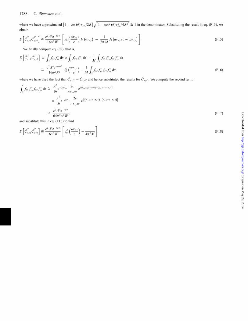
1788 C. Weemstra et al.
where we have approximated[1 − cos (θ ) rxy/2R
]√[1 − cos2 (θ ) r 2
xy/4R2] ∼= 1 in the denominator. Substituting the result in eq. (F13), we
obtain
E[C
T
xy I CT
yy I
] ∼= c2 A4e−4αR
16ω2 R2
[J0
(ωrxy
c
)I0
(αrxy
) − 1
2π MJ0
(ωrxy/c − iαrxy
) ]. (F15)
We finally compute eq. (39), that is,
E[C
T
xx I CT
yy I
]=
∫S
fsx f ∗sy ds ×
∫S
fs′ y f ∗s′x ds′ − 1
M
∫S
fsx f ∗sx fsy f ∗
sy ds
∼= c2 A4e−4αR
16ω2 R2J 2
0
(ωrxy
c
)− 1
M
∫S
fsx f ∗sx fsy f ∗
sy ds, (F16)
where we have used the fact that C yxC = C xyC and hence substituted the results for C xyC . We compute the second term,∫S
fsx f ∗sx fsy f ∗
sy ds ∼= A2
16e−2αrsx
2c
πrsxωei[(rsx ω/c−π/4)−(rsx ω/c−π/4)]
× A2
16e−2αrsy
2c
πrsyωei[(rsyω/c−π/4)−(rsyω/c−π/4)]
∼= c2 A4e−4αR
64π 2ω2 R2, (F17)
and substitute this in eq. (F16) to find
E[C
T
xx I CT
yy I
] ∼= c2 A4e−4αR
16ω2 R2
[J 2
0
(ωrxy
c
)− 1
4π 2 M
]. (F18)
by guest on May 29, 2014
http://gji.oxfordjournals.org/D
ownloaded from