Introduction to Dyna

Computational Linguistics

July 3, 2013

1 What is Dyna?

Dyna is a simple and straightforward programming language that you’ll be using in theassignments for this course. It’s being developed at Johns Hopkins by Prof. Jason Eisner,Nathaniel Wesley Filardo, and Tim Vieira, among other contributors.

If you have any experience programming, then Dyna will probably look very differentfrom other languages you’ve seen. That’s because Dyna is very high-level, and because it’sa declarative language. The rest of this section explains what those terms mean, for thosewho are curious. You’re also welcome to skip directly to Section 2, which explains the basicsof Dyna and shows you some simple examples. After that, Section 3 shows you how to useDyna to compute unigram and bigram probabilities from a corpus.

1.1 High-Level Languages

A high-level language is a programming language where the computer does much of thework for you. High-level languages abstract away from the messy details; the higher-level aprogramming language is, the more levels of abstraction it will contain.

When computer science first began, only very low-level languages existed. In the lowest-level languages, called assembly languages, programmers had to provide a detailed set ofinstructions for the computer to follow. In order to add two numbers, for instance, theprogrammer might have to write something that looked like “load the first number frommemory location X; load the second number from memory location Y; add them together;store the result in memory location Z”.

As you might imagine, these kinds of programs were quite cumbersome to write, andso programmers developed higher-level languages that could abstract away some of thesedetails. In these languages, a compiler or interpreter is used to translate from high-levelinstructions down into low-level assembly language commands. The compiler or interpreter’schallenge is to find the most efficient low-level instructions that it can. This is harder forhigher-level languages, since the compiler has to do more translation to get the programsdown to assembly code. But over time, as compilers have gotten smarter and computers havegotten faster, programmers have been able to switch to progressively higher-level languageswithout needing to worry about efficiency. More and more messy details of the programmingprocess have been abstracted away.

To give you some examples, C is an old compiled language that is still widely used. It’shigher-level than assembly, because you can write “Z = X + Y” instead of the sequenceof load/add/store instructions shown above, but you still have to deal with some memorymanagement. Languages like Java and Python are higher-level than C. In both Java and

1

Python, you don’t need to worry about managing the memory explicitly, and a lot of commonprogramming tools (for instance data structures like lists, hash tables, and sets) are builtin. The highest-level language of all would be a natural language; you would simply tell thecomputer, in English, what you wanted the program to do, and the compiler would go off,with no further effort on your part, and figure out how to do what you asked.

“Programming” using plain English will have to wait until we’ve solved NLP, but in themeantime, a language like Dyna is about as close as you’re going to get. In Dyna, if youwant to know the value of something, you don’t need to give explicit instructions on how tocompute it. You just describe what the value looks like, and the Dyna interpreter will figureout on its own how to find it efficiently. We realize this is a bit vague; you’ll see exampleslater in the tutorial. In particular, if you’ve encountered Dijkstra’s algorithm for findingthe shortest path in a graph, you may be surprised to learn that the Dyna version can bewritten in just three lines.

1.2 Declarative Languages

Dyna is a declarative language. Declarative programming is one of many programmingparadigms. Like high-level vs. low-level, programming paradigms are another way in whichlanguages can differ from one another. When you write a program, you are asking thecomputer to calculate a specific answer for you. Different programming paradigms expressthis request in different ways.

If you have any programming experience, then you’ve probably encountered the imper-ative paradigm. In this paradigm, a program is a list of instructions that the computerneeds to execute: “while condition is true, do something”. There’s also the object-orientedparadigm, used by languages like Java, where computation involves the creation and manip-ulation of objects. Languages like Lisp and Haskell follow the functional paradigm, whereeverything is expressed in terms of functions.

And Dyna follows the declarative paradigm, where instead of giving the computer in-structions, you just describe what the solution looks like. Instead of telling the computerhow to do something, you just tell it what you want it to compute, and it figures out the“how” part for you. For example, in most languages, if you want to sort a list of values,you’ll need to write out a sorting algorithm like bubblesort or mergesort. In a declarativelanguage, you might specify list sorting as follows:

given a list L, find a new list M such that:

- M is a permutation of L

- M’s elements appear in sorted order

The compiler would need to figure out a sorting algorithm on its own. As you mightimagine, declarative languages are necessarily very high-level, and writing efficient compil-ers/interpreters for them is quite challenging.

Jason teaches a whole course on declarative languages, so if you’re curious, make sureto check out the website: http://cs.jhu.edu/~jason/325/.

2

2 The Basics of Dyna

This section will explain the basics of Dyna. You’re encouraged to follow along with thetutorial by trying everything out yourself.

To use Dyna, first log into your account on the CLSP server. When you’re on themachine a14, type dyna at the command line (it might take a few seconds to load). Youwill then see the Dyna prompt.

username@a14:~$ dyna

>

To exit Dyna, you can type exit at the Dyna prompt:

> exit

username@a14:~$

2.1 Defining Items in Dyna

Dyna is a lot like a (very powerful) spreadsheet. In a spreadsheet, you have cells, and youcan give them values in two ways: by assigning them values directly, or by defining them interms of other chart cells. For instance, you might define the cell C1 to be the sum of cellsA1 and B1, whose values you have typed in by hand.

Let’s try this in Dyna. The Dyna equivalent of a chart cell is called an item. So let’screate three items in Dyna, called a, b, and c. First we’ll define a and b:

> a := 5.

Changes

=======

a = 5.

> b := 7.

Changes

=======

b = 7.

Note: to follow along with this tutorial, whenever you see a line that starts with theprompt >, you can type in the part of the line which follows the prompt (and then pressenter). Every line that does not begin with > is a reply from the Dyna intepreter. So, inthis example, you can enter the line a := 5., and Dyna will respond to it and then giveyou another prompt, at which point you can type b := 7.

The lines of Dyna code that we typed (a := 5. and b := 7.) are called rules. Eachtime you type a rule into Dyna, the interpreter tells you which values have been updated asa result. In the case of a := 5. the value of a has been updated to 5. (Previously, a didn’teven exist, and so it had no value.)

Now let’s define c as the sum of a and b:

3

> c += a + b.

Changes

=======

c = 12.

This rule is similar to the previous two, but as you can see, the first two rules defined a

and b using numeric values, while this rule defines c in terms of other Dyna items.You’ll also notice that the first two rules use :=, while the last rule uses +=. These are

called aggregators. Each Dyna rule helps to define the value of an item. The item appearsto the aggregator’s left, and a contribution to its value appears to the aggregator’s right.

A single item may appear on the left of many rules, so it may get many contributions.The aggregator specifies how to aggregate (combine) those contributions into a single valuefor the item. The aggregator += says to add up the contributions, so each += rule says“augment this item’s definition by adding in this new contribution”. The aggregator :=

says to use the last contribution only, so each := rule says “redefine this item to equal thisnew contribution”.

When there is only one contribution to an item, it usually doesn’t matter how thecontributions are aggregated. So the rules above just define a, b, and c to each equal asingle contribution. But we’ll see examples later on where += and := do have differenteffects; we’ll also see different aggregators.

2.1.1 Watch Out for Errors

Make sure to end your rules with a period, or you’ll get an error:

> a := 5

ERROR: Line doesn’t end with period.

It’s also important to get the syntax of the rule correct. A rule in Dyna should containthese five things in this order:

• an item (such as a)

• an aggregator (such as +=)

• a value (such as 5), oran expression which has a value (such as a + b)

• an optional condition (we haven’t seen these yet)

• a period to end the line

This means that you can’t, for instance, type 5 := a. If you do this, it will confuse Dynagreatly:

4

> 5 := a.

DynaCompilerError:

Terribly sorry, but you’ve hit an unsupported feature

This is almost assuredly not your fault! Please contact a TA.

The rule at <repl> is beyond my abilities.

new rule(s) were not added to program.

(Actually, this would be your fault, but Dyna errs on the side of friendliness. And if youare having trouble writing a program in Dyna, you are always welcome to contact a TA.)

2.1.2 Dyna is Dynamic

Now let’s return to our example. We’ve defined three items, a, b, and c. The item c isdefined in terms of a and b. Like a spreadsheet, Dyna is dynamic, so if you change thevalue of a or b, c changes accordingly:

> a := 1.

Changes

=======

a = 1.

c = 8.

Again, after you type a rule into Dyna, it prints out all the items whose values havebeen updated. This time two items’ values were updated, a and c.

2.1.3 Defining an Item over Multiple Lines

Earlier, we defined c in one line, like this:

c += a + b.

But we also could have defined it in two lines, like this:

c += a.

c += b.

The += aggregator is designed to be used in multi-line definitions like this. Recall thateach time you use +=, it updates the item’s value by adding the new value into it.

It may seem strange to define c over two lines instead of one. In Section 2.2, you’ll seean example of why this ability is useful. It turns out that it makes the += aggregator (andall the other aggregators) very powerful. In fact, this is why they’re called aggregators: theyaggregate a collection of rules into a single definition for an item.

5

2.1.4 Retracting a Rule

Suppose we want to try changing the definition of c from

c += a + b.

to

c += a.

c += b.

as shown in the previous section. We can’t just type in the rules from the second box,because c already has the value a + b, and adding more rules will just add to this value:

> c += a.

Changes

=======

c = 9.

> c += b.

Changes

=======

c = 16.

So what do we do if we want to switch c’s definition to the new version? We have toretract the rule c += a + b. We can do this using the retract_rule command in Dyna:

> retract_rule X

Here, X is the index of the rule you want to retract. You can find out a rule’s index bytyping the command rules, which lists all the rules that have been defined so far.

> rules

Rules

=====

0: a := 5.

1: b := 7.

2: c += a + b.

3: a := 1.

4: c += a.

5: c += b.

From this, we know that we want to retract rule 2:

6

> retract_rule 2

Changes

=======

c = 8.

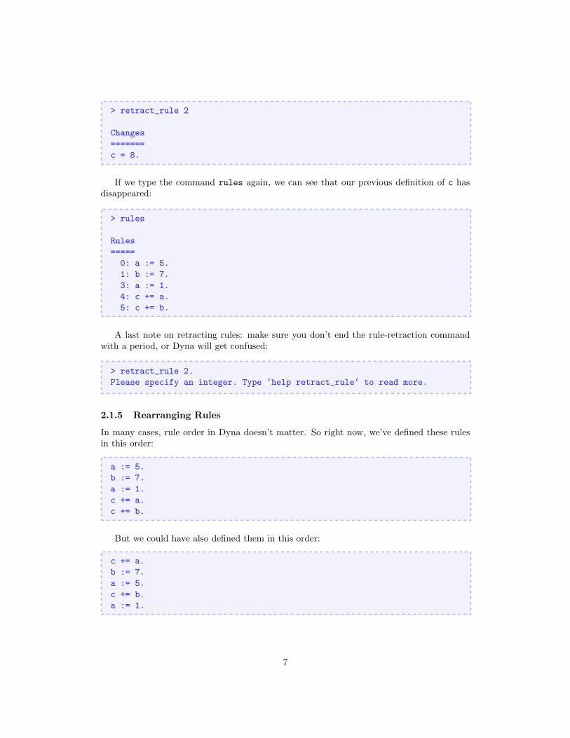
If we type the command rules again, we can see that our previous definition of c hasdisappeared:

> rules

Rules

=====

0: a := 5.

1: b := 7.

3: a := 1.

4: c += a.

5: c += b.

A last note on retracting rules: make sure you don’t end the rule-retraction commandwith a period, or Dyna will get confused:

> retract_rule 2.

Please specify an integer. Type ‘help retract_rule‘ to read more.

2.1.5 Rearranging Rules

In many cases, rule order in Dyna doesn’t matter. So right now, we’ve defined these rulesin this order:

a := 5.

b := 7.

a := 1.

c += a.

c += b.

But we could have also defined them in this order:

c += a.

b := 7.

a := 5.

c += b.

a := 1.

7

Here, we’ve made a number of changes. For one thing, we’ve switched the order of therules a := 5. and b := 7.. Unsurprisingly, this doesn’t affect their values.

What might be more surprising is that we can move the rule c += a. to the beginning,before a is even defined. (We could have also moved the rule c += b. to the beginning ifwe had wanted to.)

How does this work? Well, when we first type c += a., a’s value is undefined. Thismeans that c is the sum of something undefined, making c’s value undefined as well. Butnot for long! As soon as we add the rule a := 5., then c’s value, which depends on thevalue of a, gets updated. (The addition of the rules c += b. and a := 1. also update thevalue of c, of course.)

To make this clear, let’s retract all the rules we added before, and now add them in thenew order. This is what Dyna prints out:

> c += a.

> b := 7.

Changes

=======

b = 7.

> a := 5.

Changes

=======

a = 5.

c = 5.

> c += b.

Changes

=======

c = 12.

> a := 1.

Changes

=======

a = 1.

c = 8.

As you can see, some of the intermediate values are different. In particular, Dyna printsnothing after we add c += a. That’s because nothing has changed, since c’s value wasundefined before we added the rule, and it’s undefined after we’ve added the rule too.

The important thing to note is that the final result remains unchanged. These five rules,taken together as a set, define the values of a, b, and c. For the most part, reordering therules within the set won’t affect the values.

The big exception is the := aggregator. It defines an item’s value as the last rule thatapplies to that item. So, if we had switched the order of the a rules like this:

8

a := 1.

a := 5.

then a’s final value would be 5, and c’s value would reflect this as well.A final note on terminology: a, b, and c are all terms. When a term has a value, we

call it an item. When a term’s value is undefined, we say that the term has the value null.

2.2 Items with Variables

As we said at the beginning, Dyna is a lot like a very powerful spreadsheet. But an Excelspreadsheet has a fixed 2D structure of rows and columns. This means that every cell in aspreadsheet is defined in terms of a letter and a number, e.g. A1 or H75.

A Dyna program, on the other hand, is not restricted in this way. So far, we’ve seenitems named a, b, c, and you can also have longer names like sum and veryLongName. Butall of these names are just plain strings of text. Often, you will want to define more complexnames, to give your items more structure:

> d(1) := 5.

Changes

=======

d(1) = 5.

> d(2) := 10.

Changes

=======

d(2) = 10.

> d(3) := 19.

Changes

=======

d(3) = 19.

In this example, d is called a functor. The functor d takes one argument. Functorsmake it possible to refer to many items at the same time:

> dtotal += d(I).

Changes

=======

dtotal = 34.

As you can see, this rule adds up d(1), d(2), and d(3). How does it do this? Itturns out that the rule dtotal += d(I). doesn’t just describe a single addition to dtotal’s

9

value, but a whole set of additions, one for each item that pattern-matches to d(I). I isa variable that will match any argument of the functor d. So, in this example, the linedtotal += d(I). is equivalent to the following three rules:

dtotal += d(1).

dtotal += d(2).

dtotal += d(3).

But this takes a lot longer to write, and is much less general. With the original definition,if we added a new item d(4), it would automatically update dtotal:

> d(4) := 6.

Changes

=======

d(4) = 6.

dtotal = 40.

This wouldn’t work for the three-line definition. You’d have to add a new line like this:

dtotal += d(4).

The rule dtotal += d(I). is much like the mathematical equation dtotal =∑

I d(I),while using three separate rules is like writing dtotal = d(1) + d(2) + d(3). If d(4) is defined,the first equation would include it in the sum automatically, while the second equation qouldignore it.

In the next section, we’ll look at some more examples with variables. First, though,how can we tell a variable from a functor? It’s easy: a variable always starts with a capitalletter, and a functor always starts with a lowercase letter.

So, earlier, we wrote dtotal += d(I). If we now write dtotal2 += d(a), we will seethat it gives a completely different answer:

> dtotal2 += d(a).

Changes

=======

dtotal2 = 5.

What happened here? Well, a is a functor, not a variable. Recall from earlier that a hasthe value 1. So, in this example, a evaluates to 1, and thus d(a) becomes equal to d(1),which equals 5.

Exercise: What does d(2*a+1) evaluate to?

10

2.2.1 Some More Examples with Variables

Here’s another example containing a Dyna rule with a variable:

e(1) := 1.

e(2) := 2.

f(1) := 4.

f(2) := 5.

g += e(I)*f(I).

This turns out to be equivalent to:

g += e(1)*f(1).

g += e(2)*f(2).

That is, the variable I appears twice in g += e(I)*f(I)., so both instances of I have topattern-match to the same thing. That’s because the rule is saying “for all I such that e(I)and f(I) are defined, add e(I)*f(I) to the definition of g”. (Note: the * is a multiplicationsign.)

If you use two different variables, the result will be different, because the variables canpattern-match independently:

h += e(I)*f(J).

This is equivalent to:

h += e(1)*f(1).

h += e(1)*f(2).

h += e(2)*f(1).

h += e(2)*f(2).

In other words, the rule h += e(I)*f(J). says “for all I, J pairs such that e(I) andf(J) are both defined, add e(I)*f(J) to the definition of h”.

2.2.2 Functors with Multiple Arguments

So far, we’ve seen functors with one argument, such as d(1). We’ve also seen functors withzero arguments — it turns out that the items a, b, and c that we defined at the beginningare actually just functors with no arguments. a is equivalent to a(), but Dyna allows youto leave out the parentheses for zero-argument functors, to make them easier to type.

Of course, in Dyna, you aren’t limited to zero- or one-argument functors. You can definefunctors with as many arguments as you like. For instance, if you were making the Dynaequivalent of a grading spreadsheet, you might have a functor with two arguments that listseach student’s grade on each exam:

11

grade("Steve", "midterm") := 85.

grade("Steve", "final") := 90.

grade("Jamie", "midterm") := 94.

grade("Jamie", "final") := 97.

grade("Anna", "midterm") := 82.

grade("Anna", "final") := 89.

Now suppose we want to compute each student’s total score. Also, to make things moreinteresting, suppose that the two exams are weighted differently. So let’s add a new functorspecifying the percent each exam contributes to the student’s final grade in the class.

weight("midterm") := 0.35.

weight("final") := 0.65.

Then we can compute the final grade for each student like this:

finalgrade(I) += grade(I,J)*weight(J).

The names of the variables don’t matter; we’ve just chosen I and J because they’reconventional variable names. But often, you’ll want to choose more meaningful variablenames to make your rules more readable. The following rule is equivalent to the previousone:

finalgrade(Student) += grade(Student,Exam)*weight(Exam).

We can also have rules which contain both variables and atoms. (An atom is an argu-ment to a functor. Types of atoms include strings in quotes, like "Steve", and numbers,like 903 or 3.14159. Variables don’t count as atoms, because they stand in place of atoms.)For an example of a rule which contains both variables and atoms, suppose we only wantedto compute Steve’s grade, and we didn’t care about Jamie or Anna. Then we could use thefollowing rule:

finalgrade("Steve") += grade("Steve",Exam)*weight(Exam).

So now we’ve seen functors with zero, one, and two arguments. But remember, functorscan have as many arguments as you like:

> x(1,2,3,4,5,6,7,8,9,"panda") := 2.

Changes

=======

x(1,2,3,4,5,6,7,8,9,"panda") := 2

12

Also, it’s important to note that the same functor can appear with different numbers ofarguments. So, instead of

finalgrade(Student) += grade(Student,Exam)*weight(Exam).

we could have written

grade(Student) += grade(Student,Exam)*weight(Exam).

Now we have two versions of the functor grade, one with one argument and anotherwith two arguments. This is similar to how the English verb “eat” has both intransive andtransitive versions.

Note that these two versions of grade don’t interfere with each other during patternmatching, since any use of grade must either pattern match to the one-argument version orthe two-argument version, but it can’t pattern match to both at the same time. So supposewe say:

allgrades += grade(Student).

This rule can only match the one-argument version of grade.

2.3 Writing a Program in Dyna

We’ve seen a lot of basic examples in this section, and we’re almost ready to move on toreal NLP applications. First, though, you’ll need to know how to write an actual programin Dyna. So far, we’ve just been typing rules directly into the Dyna interpreter. This isvery useful for playing around with Dyna, but it’s quite inconvenient if you want to runthe same program more than once. You would have to retype the rules into the interpreterevery time you wanted to run it.

Fortunately, you can save your rules in a file, and Dyna will read them. For instance,open up your favorite command line text editor (e.g. nano, vim, emacs), and type the rulesfrom our grading example:

grade("Steve", "midterm") := 85.

grade("Steve", "final") := 90.

grade("Jamie", "midterm") := 94.

grade("Jamie", "final") := 97.

grade("Anna", "midterm") := 82.

grade("Anna", "final") := 89.

weight("midterm") := 0.35.

weight("final") := 0.65.

finalgrade(Student) += grade(Student,Exam)*weight(Exam).

13

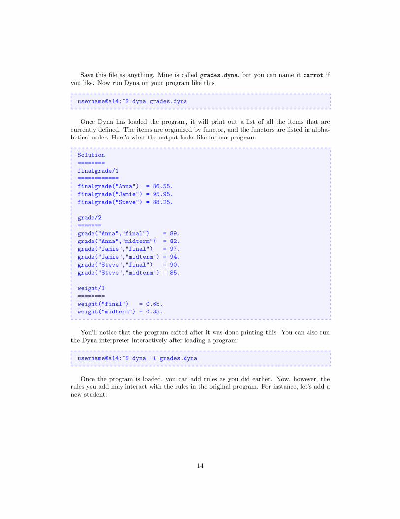
Save this file as anything. Mine is called grades.dyna, but you can name it carrot ifyou like. Now run Dyna on your program like this:

username@a14:~$ dyna grades.dyna

Once Dyna has loaded the program, it will print out a list of all the items that arecurrently defined. The items are organized by functor, and the functors are listed in alpha-betical order. Here’s what the output looks like for our program:

Solution

========

finalgrade/1

============

finalgrade("Anna") = 86.55.

finalgrade("Jamie") = 95.95.

finalgrade("Steve") = 88.25.

grade/2

=======

grade("Anna","final") = 89.

grade("Anna","midterm") = 82.

grade("Jamie","final") = 97.

grade("Jamie","midterm") = 94.

grade("Steve","final") = 90.

grade("Steve","midterm") = 85.

weight/1

========

weight("final") = 0.65.

weight("midterm") = 0.35.

You’ll notice that the program exited after it was done printing this. You can also runthe Dyna interpreter interactively after loading a program:

username@a14:~$ dyna -i grades.dyna

Once the program is loaded, you can add rules as you did earlier. Now, however, therules you add may interact with the rules in the original program. For instance, let’s add anew student:

14

> grade("Keith","midterm") := 76.

Changes

=======

finalgrade("Keith") = 26.599999999999998.

grade("Keith","midterm") = 76.

> grade("Keith","final") := 87.

Changes

=======

finalgrade("Keith") = 83.15.

grade("Keith","final") = 87.

As you can see, when we add grade("Keith","midterm"), it creates an itemfinalgrade("Keith"), using the rules finalgrade(Student) += grade(Student,Exam)*

weight(Exam). and weight("midterm") := 0.35. in the program we loaded.Now observe what happens when we add the following rule:

> grade("Vanessa", "makeup midterm") := 100.

Changes

=======

grade("Vanessa","makeup midterm") = 100.

As you can see, it does not create an item finalgrade("Vanessa"). Why is this? Con-sider what happens when the rule finalgrade(Student) += grade(Student,Exam)*weight(Exam).

tries its pattern-matching on grade("Vanessa", "makeup midterm"). The variable Studentbinds to "Vanessa" and the variable Exam binds to "makeup midterm". But there’s no itemweight("makeup midterm") in our program, so the overall pattern-matching fails.

2.3.1 What is a Dyna Program?

We are finally in a position to state what a Dyna program actually is. A Dyna program issimply a list of rules which define a set of items. (As we saw earlier, an item may be definedusing multiple rules.)

When you use the Dyna interpreter, you are slowly specifying a Dyna program, one ruleat a time. If you’re using the Dyna interpreter with a program that you loaded from file,then each rule you type into the interpreter extends that program.

Note that when you close the Dyna interpreter, it doesn’t save any of the rules that youtyped. They exist for that session only and don’t affect the original program. So if you lookat the file grades.dyna, you will see that it contains no mention of Keith or Vanessa.

2.4 The Help Command

One final note before we continue on to the next section. We have covered some commandsalready in this tutorial, and we will cover more in the next section, but we won’t have

15

time to explain every feature of Dyna. Fortunately, Dyna contains documentation whichwill help you if you don’t understand how to use a command. To see which commands aredocumented, you can type help at the Dyna prompt like this:

> help

Documented commands (type help <topic>):

========================================

EOF exit load post query retract_rule rules run sol trace vquery

Undocumented commands:

======================

help

To get help for a specific command, you can type help followed by that command’sname:

> help exit

Exit REPL by typing exit or control-d. See also EOF.

3 Counting Words in a Corpus

In this section, we’ll use Dyna to calculate unigram and bigram probabilities for a very smallsubset of the Brown corpus.

3.1 The Brown Corpus

First, let’s take a look at the corpus. We’ve stored it in a file called brown.txt, which youcan get by typing the following command:

wget http://cs.jhu.edu/~jason/licl/brown.txt

(The wget command retrieves a file from the internet, specified by its URL.)In order to look at the file’s contents, you can use this command:

username@a14:~$ less brown.txt

(The program less allows you to scroll up and down through a long piece of text to seewhat’s in it. You can type q to quit less and return to the command line.)

As you can see, the file contains lines like this:

You should hear the reverence in Fran’s voice when she said ‘‘ Baccarat

’’ or ‘‘ Steuben ’’ or ‘‘ Madame Alexander ’’ .

16

This looks like an ordinary sentence, except that something strange has happened to thepunctuation. That’s because this sentence has been tokenized, which means that it’s beensplit into meaningful units that the computer can process more easily. If we’re countingup the occurrences of the word “house” in the corpus, for instance, we don’t want to haveto consider “house” and “house,” and “house.”. (Note that tokenization is not as simpleas just detaching punctuation from words. For instance, we can’t just make a rule thatseparates all periods, because we want them to stay attached in titles like “Dr.”.)

Different tasks will call for different kinds of tokenization. Some corpora will separateout the possessive clitic, so “Fran’s” in the above sentence would be “Fran ’s”. One couldalso tokenize the corpus by morpheme instead of word.

People who are creating or using corpora might use other preprocessing techniquesas well. Many corpora remove the capitalization from the beginning of the sentence; theBrown corpus hasn’t done this.

3.2 Loading the Brown Corpus into Dyna

Now we need to load the corpus into Dyna. Fortunately, Dyna has a feature called loaderswhich makes this very easy.

In order to load our small subset of the Brown corpus, you can type the following intothe Dyna interpreter:

> load brown = matrix("brown.txt", astype=str)

If you type sol at the Dyna prompt like this:

> sol

then Dyna will print out a full list of all the items and their values. If you do this, you cansee that the data we loaded is very long, and that the bottom looks like this:

17

...

brown(1052,0) = "From".

brown(1052,1) = "what".

brown(1052,2) = "I".

brown(1052,3) = "was".

brown(1052,4) = "able".

brown(1052,5) = "to".

brown(1052,6) = "gauge".

brown(1052,7) = "in".

brown(1052,8) = "a".

brown(1052,9) = "swift".

brown(1052,10) = ",".

brown(1052,11) = "greedy".

brown(1052,12) = "glance".

brown(1052,13) = ",".

brown(1052,14) = "the".

brown(1052,15) = "figure".

brown(1052,16) = "inside".

brown(1052,17) = "the".

brown(1052,18) = "coral-colored".

brown(1052,19) = "boucle".

brown(1052,20) = "dress".

brown(1052,21) = "was".

brown(1052,22) = "stupefying".

brown(1052,23) = ".".

Each item in the data takes the form brown(Sentence,Position), and its value is theword at that position of that sentence. (The indices start at 0, so the first word in thissentence is brown(1052,0), not brown(1052,1). Similarly, words in the first sentence takethe form brown(0,Position).)

Now let’s look at the load command in more detail. Recall that it looks like this:

> load brown = matrix("brown.txt", astype=str)

The word load at the beginning tells Dyna that we want to use a loader. brown is thename of the functor to load the data into. If we had typed load red = ... instead, wewould have gotten items that looked like red(1052,0) and so on. matrix is the name of thespecific loader we are using; it loads each word as a separate item. As you might imagine,"brown.txt" tells Dyna which file to load. Lastly, astype=str tells Dyna to treat the wordsin the file as strings, and not, for instance, as numbers.

You may also find the tsv loader useful at some point. Instead of loading each wordas an item, it loads each line as an item. For instance, suppose you had a text file whichcontained the rules of a context free grammar, along with their probabilities:

18

1 S NP VP

0.5 ROOT S .

0.25 ROOT S !

0.25 ROOT VP !

0.5 VP V

0.5 VP V NP

...

In this (imaginary) file, the first column is the probability, the second column is theleft-hand side of the rule, and the remaining columns form the right-hand-side of the rule.You could load in this data using tsv like this:

> load grammar_rule = tsv("grammar.txt")

> sol

grammar_rule/4

==============

grammar_rule(4,"0.5","VP","V") = true.

grammar_rule/5

==============

grammar_rule(0,"1","S","NP","VP") = true.

grammar_rule(1,"0.5","ROOT","S",".") = true.

grammar_rule(2,"0.25","ROOT","S","!") = true.

grammar_rule(3,"0.25","ROOT","VP","!") = true.

grammar_rule(5,"0.5","VP","V","NP") = true.

...

There are a few things to note. First of all, the words in the file must be separatedby tabs in order for tsv to work. (This is why the loader is called tsv — it’s a standardabbreviation for “tab-separated values”.) Secondly, since the rules of this grammar havedifferent numbers of nonterminals, we get two versions of the grammar_rule functor, onewith four arguments and another with five. Lastly, the first argument to the functor isalways the row number in the file.

We will not actually be using tsv in this tutorial, but you may find it helpful for yourhomework.

3.3 Counting Words

Now that we’ve loaded the corpus using the matrix loader, we can use Dyna to collect theunigram counts (that is, we’ll determine how many times each word appears in the corpus):

count(W) += 1 for W is brown(Sentence,Position).

(We’ll explain how this rule works in Section 3.5, so don’t worry if it doesn’t make anysense.)

19

When you enter this rule, Dyna prints out a long list containing the count for each wordtype that appears in the corpus. The bottom of the list should look like this:

...

count("written") = 1.

count("wrong") = 2.

count("wrote") = 7.

count("wry") = 1.

count("yapping") = 1.

count("yaws") = 1.

count("year") = 8.

count("yearly") = 1.

count("yearning") = 1.

count("years") = 21.

count("yelled") = 1.

count("yellow") = 1.

count("yelping") = 1.

count("yes") = 1.

count("yet") = 3.

count("yore") = 1.

count("you") = 131.

count("you’ll") = 1.

count("you’re") = 9.

count("you’ve") = 4.

count("young") = 4.

count("youngest") = 1.

count("your") = 38.

count("yours") = 2.

count("yourself") = 1.

count("yourselves") = 4.

count("youth") = 2.

count("zounds") = 2.

These counts might seem a bit strange. The word “yore” appears just as often as“yourself” does, for instance. That’s because we used a very small subset of the Browncorpus (just 1053 sentences). The smaller the corpus, the less reliable the counts will be.With only 1053 sentences, it’s no wonder that we find some anomalies! But in a corpus ofa million sentences, it’s very unlikely that we’d still see “yore” as frequently as “yourself”.

By the way, in Computational Linguistics terminology, the brown(Sentence,Position)

items represent word tokens while the count(W) items range over word type. A token is aspecific instance of a generic word type. For instance, brown(1052,14) and brown(1052,17)

both have the value “the”. These two items represent two different tokens, but only oneword type.

3.4 Querying Dyna

As you’ve presumably noticed, the list of counts that Dyna printed is very long. What ifyou wanted to know the count of the word and? Would you have to scroll all the way up tothe top of the list?

20

It turns out that Dyna has a more convenient way of checking an item’s value, called aquery:

> query count("and")

count("and") = 512

Queries are very simple. You just type the word query followed by the item whose valueyou want to know, and Dyna will print that value.

If you query an item that doesn’t exist or has no contributions, Dyna will inform youthat there are no results:

> query pajamas

No results.

You can also make more complicated queries, where you ask Dyna for the value of awhole expression, instead of just a single item:

> query count("year") + count("years")

count("year") + count("years") = 29

Note that while rules end with a period, queries do not:

> query count("year") + count("years").

Queries don’t end with a dot.

Like rules, queries can contain variables. The following query would show us the countof every word:

> query count(W)

We can also mix atoms and variables in queries, just as we did with rules:

21

> query brown(57,Position)

brown(57,0) = "With"

brown(57,1) = "greater"

brown(57,10) = "this"

brown(57,11) = "time"

brown(57,12) = "a"

brown(57,13) = "little"

brown(57,14) = "more"

brown(57,15) = "to"

brown(57,16) = "the"

brown(57,17) = "left"

brown(57,18) = "."

brown(57,2) = "precision"

brown(57,3) = "he"

brown(57,4) = "again"

brown(57,5) = "paced"

brown(57,6) = "off"

brown(57,7) = "a"

brown(57,8) = "location"

brown(57,9) = ","

As you can see, this shows us the entirety of sentence 57, albeit not in the correct order.We can also view the first word of each sentence using the following query:

> query brown(Sentence,0)

3.5 Rules with Conditions

Let’s return to our word-counting rule, and look at the details of how it works. Recall thatthe rule looks like this:

count(W) += 1 for W is brown(Sentence,Position).

This is our first example of a rule with a condition. The condition tells you when therule should apply. In this case, it applies once for each word token in the corpus, because eachtoken will pattern-match to a different brown(Sentence,Position) item. You can think ofthis rule as saying “For each Sentence and Position such that brown(Sentence,Position)is defined, let W be the value of brown(Sentence,Position), and add 1 to count(W).”

How does this rule work, exactly? A condition contains the word for followed by aboolean expression (that is, an expression whose value is either true or false). The ex-pression count("year") + count("years") is not a boolean, since its value is the number29. The expression count("year") > count("years"), on the other hand, is a booleanwhose value is false:

22

> query count("year") > count("years")

count("year") > count("years") = false

Returning again to our word-counting rule, the expression W is brown(Sentence,Position)

is true when W is the value of brown(Sentence,Position). For instance, "what" is the valueof brown(1052,1), so the expression W is brown(1052,1) is true when W pattern-matchesto "what".

For a slightly more complicated example, suppose you only wanted the counts of thewords from the first 50 sentences of the corpus. You would have to add an extra restrictionto the condition:

count2(W) += 1 for (W is brown(Sentence,Position)) & (Sentence < 50).

Now, an item of the form brown(Sentence,Position) won’t pattern-match this ruleunless Sentence < 50. (Note that we put parentheses around the two conditions to keepthe Dyna parser from getting confused. If the Dyna parser is getting confused, this is onething you can try.)

Exercise: How many different word types appear in the corpus?

3.6 Creating Probabilities from Unigram Counts

Now that we have the unigram counts, we can use them to determine the unigram proba-bilities for each word in the corpus.

Recall that the unigram probability p(w) of a word w is c(w)c , where c(w) is the count

of word w, and c is the total number of word tokens in the corpus.Exercise: How can you use Dyna to count the total number of word tokens in the

corpus? (Hint: the correct number turns out to be 21695.)After completing this exercise, you can use the total count of words in the corpus to

compute the probability of each word:

unigram_prob(W) := count(W) / totalcount.

3.7 Finding the Most Frequent Word

These counts and probabilities are nice because we can use them to discover interesting factsabout the corpus. For instance, we might ask, what is the most common word? What isthat word’s frequency? What is that word’s probability?

We’ll first compute the mystery word’s frequency, using the following rule:

> highest_frequency max= count(W).

Changes

=======

highest_frequency = 1331.

23

As you can see, we’ve used a new aggregator, max=. The rule says that highest_frequency’svalue should be defined as maximum value of all the counts. That is, out of every item thatpattern-matches to count(W), max= picks the one with the highest value, and assigns thatvalue to highest_frequency. Note that there is also a similar aggregator called min= thatfinds the minimum.

The most common word in the corpus appears 1331 times. We can now use a query tocheck which word it is:

> query W for count(W) == highest_frequency

"," for count(",") == highest_frequency = ","

As you can see, the most frequent word is. . . a comma. Well, that’s pretty boring. Onthe bright side, the query we used to find it has an interesting structure. In particular, thisexample reveals that queries can contain conditions, and those conditions work exactly thesame way as they do in rules.

For another query with a condition, consider the following example, where we ask Dynato show us all rules whose counts are greater than 1000.

> query W for count(W) > 1000

"," for count(",") > 1000 = ","

Turns out it’s just the comma. If we lower the threshold to 900, we also get “the”:

> query W for count(W) > 900

"," for count(",") > 900 = ","

"the" for count("the") > 900 = "the"

Finally, to complete the example from this section, we can ask what the probability ofthe comma is:

> query unigram_prob(",")

unigram_prob(",") = 0.061350541599446876

It seems that approximately 6% of all the words in our corpus are commas.Exercise: Comma is the most common word overall. But what is the most common

word to start a sentence with?

3.8 Computing Bigram Probabilities

Now let’s compute the bigram probabilities for this corpus. First, we’ll need to collect thebigram counts:

24

in_vocab(W) := true for count(W) > 0.

bigram_count(V,W) += 0 for in_vocab(V) & in_vocab(W).

bigram_count(V,W) += 1 for (V is brown(Sentence,Position)) &

(W is brown(Sentence,Position+1)).

The third line should be the most straightforward. It increases the bigram count for thepair of words V, W whenever W follows V in the corpus (i.e. they are in the same sentenceand W’s position is V’s position plus 1).

The first and second line are a bit more complicated; they work together to make surethe count of each bigram starts out at 0. This is important because, if a bigram neverappears in the corpus, we want its count to be 0 instead of undefined.

The first line determines which words appear in the corpus. It sets in_vocab(W) to thelogical value true for each word W that appears in the corpus.

The second line adds 0 to the bigram count for each pair of words in the vocabulary.The second and third lines work together to define bigram_count(V,W). Specifically, thesecond line adds 0 to the count of each bigram that could appear in the corpus. The thirdline adds 1 whenever the bigram actually does appear.

(Unfortunately, at the time of writing this tutorial, Dyna is too slow to compute theresults of the second rule in a reasonable amount of time. When we tried this rule out, wegot tired of waiting for Dyna, and so we typed Ctrl-C, which tells Dyna to cancel whateverit’s currently doing.

Why is Dyna so slow here? Well, there are 5017 word types in the corpus, meaningthat there are approximately 50172 = 25170289 possible bigrams. Dyna naively tries tocompute zeros for all of these. The right approach would be to compute only the countsof bigrams that actually occur, and simply return zero by default for any other bigram. Afuture version of Dyna will be able to figure that out.)

Now that we have the bigram counts, we can use them and the original counts to computethe bigram probabilities:

bigram_prob(V,W) := bigram_count(V,W) / count(V).

As you can see, “the man” has a probability of around 0.002, while “man the” has aprobablity of 0, because it never appears in this corpus and we haven’t used any smoothing:

> query bigram_prob("the","man")

bigram_prob("the","man") = 0.002150537634408602

> query bigram_prob("man","the")

bigram_prob("man","the") = 0

Exercise: What word is most likely after “the”, and how likely is it? What word ismost likely after “of”? How about before “.”?

Exercise: Define estimates of bigram probabilities that use add-λ smoothing. (Hint:define lambda := 1 and write your defs in terms of lambda. You can change lambda and

25

the estimated probabilities will change as well.) Can you compute cross-entropy on a devel-opment corpus?

Exercise: Using a similar approach to the one in this section, compute the trigramprobabilities.

3.9 VQuery and Trace

We’ve now seen many examples of queries, both with and without conditions. In additionto the query command, Dyna also has two other commands that you might find helpful:vquery and trace.

The regular query is designed for querying the value of an expression. On the other hand,vquery is designed for investigating the variables that pattern-match to an expression.

To see the difference, suppose you want to know which bigrams have a count greaterthan zero, and what their counts are. You could use a regular query like this:

> query bigram_count(V,W) for bigram_count(V,W) > 0

and it will spew something ugly like this:

...

bigram_count("yourself","to") for bigram_count("yourself","to") > 0 = 1

bigram_count("yourselves",",") for bigram_count("yourselves",",") > 0 = 1

bigram_count("yourselves","into") for bigram_count("yourselves","into") > 0 = 1

bigram_count("yourselves","of") for bigram_count("yourselves","of") > 0 = 1

bigram_count("yourselves","on") for bigram_count("yourselves","on") > 0 = 1

bigram_count("youth","is") for bigram_count("youth","is") > 0 = 1

bigram_count("youth","worked") for bigram_count("youth","worked") > 0 = 1

bigram_count("zounds","’’") for bigram_count("zounds","’’") > 0 = 2

Or you could use vquery, which gives a much cleaner answer, in sorted order (thoughhere, V and W are backwards):

> vquery bigram_count(V,W) for bigram_count(V,W) > 0

...

57 where W="I", V=","

76 where W="the", V=","

76 where W="?", V="?"

88 where W="the", V="in"

106 where W=",", V="’’"

111 where W=".", V="’’"

115 where W="the", V="of"

130 where W="and", V=","

Another useful command is trace, which shows where an item got its value. The follow-ing trace will tell you which sentences in the corpus contributed to the count for the bigram“through the”:

26

> trace bigram_count("through","the")

3.10 Another Way of Writing Some Rules

Earlier, to count the words in the corpus, we wrote the following:

count(W) += 1 for W is brown(Sentence,Position).

But there’s another way we could have written this rule:

count( brown(Sentence,Position) ) += 1.

What’s going on here? First, the brown(Sentence,Position) part pattern-matches toone of the words in the corpus, like brown(1052,11). So, after pattern-matching, we get arule that looks like this:

count( brown(1052,11) ) += 1.

The value of brown(1052,11) is "greedy". How does Dyna figure out that it needs toincrement the count of the word "greedy"? Well, first it has to evaluate brown(1052,11)

(i.e. replace the item with its value). After evaluating, the rule looks like this:

count("greedy") += 1.

At first, it may not be intuitive that this rule works. How does this rule get the countsright? Why doesn’t it just set each word’s count to 1 or something?

What happens is that the rule pattern-matches once for each word token in the corpus(each brown(Sentence,Position) item). So, if the word “each” appears nine times inthe corpus (which it does), then there will be nine brown(Sentence,Position) items thatevaluate to "each". This means that count("each") will be incremented nine times.

We can write a rule like this for the bigram counts also. Recall that the original rulelooked like this:

bigram_count(V,W) += 1 for (V is brown(Sentence,Position)) &

(W is brown(Sentence,Position+1)).

Our new rule will look like this:

bigram_count(brown(Sentence,Position), brown(Sentence,Position+1)) += 1.

27