Intr oductory Lectures on Quantum Field Theory · Intr oductory Lectures on Quantum Field Theory...

Introductory Lectures on Quantum Field Theory

Luis Álvarez-Gaumé a and Miguel A. Vázquez-Mozo b

a CERN, Geneva, Switzerlandb Universidad de Salamanca, Salamanca, Spain

AbstractIn these lectures we present a few topics in Quantum Field Theory in detail.Some of them are conceptual and some more practical. They have been se-lected because they appear frequently in current applications to Particle Physicsand String Theory.

1 IntroductionThese notes summarize lectures presented at the 2005 CERN-CLAF school in Malargüe, Argentina, the2009 CERN-CLAF school in Medellín, Colombia, the 2011 CERN-CLAF school in Natal (Brazil), andthe 2012 Asia-Europe-Pacific School of High Energy Physics in Fukuoka (Japan). The audience in alloccasions was composed to a large extent by students in experimental High Energy Physics with animportant minority of theorists. In nearly ten hours it is quite difficult to give a reasonable introductionto a subject as vast as Quantum Field Theory. For this reason the lectures were intended to provide areview of those parts of the subject to be used later by other lecturers. Although a cursory acquaitancewith th subject of Quantum Field Theory is helpful, the only requirement to follow the lectures it is aworking knowledge of Quantum Mechanics and Special Relativity.

The guiding principle in choosing the topics presented (apart to serve as introductions to latercourses) was to present some basic aspects of the theory that present conceptual subtleties. Those topicsone often is uncomfortable with after a first introduction to the subject. Among them we have selected:

- The need to introduce quantum fields, with the great complexity this implies.- Quantization of gauge theories and the rôle of topology in quantum phenomena. We have included

a brief study of the Aharonov-Bohm effect and Dirac’s explanation of the quantization of theelectric charge in terms of magnetic monopoles.

- Quantum aspects of global and gauge symmetries and their breaking.- Anomalies.- The physical idea behind the process of renormalization of quantum field theories.- Some more specialized topics, like the creation of particle by classical fields and the very basics

of supersymmetry.

These notes have been written following closely the original presentation, with numerous clarifi-cations. Sometimes the treatment given to some subjects has been extended, in particular the discussionof the Casimir effect and particle creation by classical backgrounds. Since no group theory was assumed,we have included an Appendix with a review of the basics concepts.

By lack of space and purpose, few proofs have been included. Instead, very often we illustrate aconcept or property by describing a physical situation where it arises. A very much expanded versionof these lectures, following the same philosophy but including many other topics, has appeared in bookform in [1]. For full details and proofs we refer the reader to the many textbooks in the subject, and inparticular in the ones provided in the bibliography [2–11]. Specially modern presentations, very muchin the spirit of these lectures, can be found in references [5, 6, 10, 11]. We should nevertheless warn thereader that we have been a bit cavalier about references. Our aim has been to provide mostly a (notexhaustive) list of reference for further reading. We apologize to those authors who feel misrepresented.

1

1.1 A note about notationBefore starting it is convenient to review the notation used. Through these notes we will be using themetric ηµν = diag (1,−1,−1,−1). Derivatives with respect to the four-vector xµ = (ct, x) will bedenoted by the shorthand

∂µ ≡ ∂

∂xµ=

(1

c

∂

∂t, ∇). (1)

As usual space-time indices will be labelled by Greek letters (µ, ν, . . . = 0, 1, 2, 3) while Latin indiceswill be used for spatial directions (i, j, . . . = 1, 2, 3). In many expressions we will use the notationσµ = (1, σi) where σi are the Pauli matrices

σ1 =

(0 11 0

), σ2 =

(0 −ii 0

), σ3 =

(1 00 −1

). (2)

Sometimes we use of the Feynman’s slash notation /a = γµaµ. Finally, unless stated otherwise, we workin natural units ℏ = c = 1.

2 Why do we need Quantum Field Theory after all?In spite of the impressive success of Quantum Mechanics in describing atomic physics, it was immedi-ately clear after its formulation that its relativistic extension was not free of difficulties. These problemswere clear already to Schrödinger, whose first guess for a wave equation of a free relativistic particle wasthe Klein-Gordon equation

(∂2

∂t2− ∇2 +m2

)ψ(t, x) = 0. (3)

This equation follows directly from the relativistic “mass-shell” identity E2 = p 2 +m2 using the corre-spondence principle

E → i∂

∂t,

p → −i∇. (4)

Plane wave solutions to the wave equation (3) are readily obtained

ψ(t, x) = e−ipµxµ= e−iEt+ip·x with E = ±ωp ≡ ±

√p 2 +m2. (5)

In order to have a complete basis of functions, one must include plane wave with both E > 0 and E < 0.This implies that given the conserved current

jµ =i

2

(ψ∗∂µψ − ∂µψ

∗ ψ), (6)

its time-component is j0 = E and therefore does not define a positive-definite probability density.

A complete, properly normalized, continuous basis of solutions of the Klein-Gordon equation (3)labelled by the momentum p can be defined as

fp(t, x) =1

(2π)32√

2ωp

e−iωpt+ip·x,

f−p(t, x) =1

(2π)32√

2ωp

eiωpt−ip·x. (7)

2

L. ÁLVAREZ-GAUMÉ AND M.A. VÁZQUEZ-MOZO

2

Energy

m

0

−m

Fig. 1: Spectrum of the Klein-Gordon wave equation.

Given the inner product

⟨ψ1|ψ2⟩ = i

∫d3x(ψ∗

1∂0ψ2 − ∂0ψ∗1 ψ2

)

the states (7) form an orthonormal basis

⟨fp|fp′⟩ = δ(p− p ′),

⟨f−p|f−p′⟩ = −δ(p− p ′), (8)

⟨fp|f−p′⟩ = 0. (9)

The wave functions fp(t, x) describes states with momentum p and energy given by ωp =√p 2 +m2.

On the other hand, the states |f−p⟩ not only have a negative scalar product but they actually correspondto negative energy states

i∂0f−p(t, x) = −√p 2 +m2 f−p(t, x). (10)

Therefore the energy spectrum of the theory satisfies |E| > m and is unbounded from below (see Fig.1). Although in a case of a free theory the absence of a ground state is not necessarily a fatal problem,once the theory is coupled to the electromagnetic field this is the source of all kinds of disasters, sincenothing can prevent the decay of any state by emission of electromagnetic radiation.

The problem of the instability of the “first-quantized” relativistic wave equation can be heuristi-cally tackled in the case of spin-1

2 particles, described by the Dirac equation(

−iβ ∂∂t

+ α · ∇ −m

)ψ(t, x) = 0, (11)

where α and β are 4 × 4 matrices

αi =

(0 iσi

−iσi 0

), β =

(0 11 0

), (12)

3

INTRODUCTORY LECTURES ON QUANTUM FIELD THEORY

3

Energy

m

−m

particle

antiparticle (hole)

photon

Dirac Sea

Fig. 2: Creation of a particle-antiparticle pair in the Dirac sea picture.

with σi the Pauli matrices, and the wave function ψ(t, x) has four components. The wave equation (11)can be thought of as a kind of “square root” of the Klein-Gordon equation (3), since the latter can beobtained as

(−iβ ∂

∂t+ α · ∇ −m

)†(−iβ ∂

∂t+ α · ∇ −m

)ψ(t, x) =

(∂2

∂t2− ∇2 +m2

)ψ(t, x). (13)

An analysis of Eq. (11) along the lines of the one presented above for the Klein-Gordon equationleads again to the existence of negative energy states and a spectrum unbounded from below as in Fig.1. Dirac, however, solved the instability problem by pointing out that now the particles are fermionsand therefore they are subject to Pauli’s exclusion principle. Hence, each state in the spectrum can beoccupied by at most one particle, so the states with E = m can be made stable if we assume that all thenegative energy states are filled.

If Dirac’s idea restores the stability of the spectrum by introducing a stable vacuum where allnegative energy states are occupied, the so-called Dirac sea, it also leads directly to the conclusion that asingle-particle interpretation of the Dirac equation is not possible. Indeed, a photon with enough energy(E > 2m) can excite one of the electrons filling the negative energy states, leaving behind a “hole” inthe Dirac sea (see Fig. 2). This hole behaves as a particle with equal mass and opposite charge thatis interpreted as a positron, so there is no escape to the conclusion that interactions will produce pairsparticle-antiparticle out of the vacuum.

In spite of the success of the heuristic interpretation of negative energy states in the Dirac equationthis is not the end of the story. In 1929 Oskar Klein stumbled into an apparent paradox when trying todescribe the scattering of a relativistic electron by a square potential using Dirac’s wave equation [12] (forpedagogical reviews see [13, 14]). In order to capture the essence of the problem without entering intounnecessary complication we will study Klein’s paradox in the context of the Klein-Gordon equation.

Let us consider a square potential with height V0 > 0 of the type showed in Fig. 3. A solution tothe wave equation in regions I and II is given by

ψI(t, x) = e−iEt+ip1x +Re−iEt−ip1x,

ψII(t, x) = Te−iEt+p2x, (14)

4


4

x

V(x)

V0Incoming

Reflected

Transmited

Fig. 3: Illustration of the Klein paradox.

where the mass-shell condition implies that

p1 =√E2 −m2, p2 =

√(E − V0)2 −m2. (15)

The constants R and T are computed by matching the two solutions across the boundary x = 0. Theconditions ψI(t, 0) = ψII(t, 0) and ∂xψI(t, 0) = ∂xψII(t, 0) imply that

T =2p1

p1 + p2, R =

p1 − p2

p1 + p2. (16)

At first sight one would expect a behavior similar to the one encountered in the nonrelativisticcase. If the kinetic energy is bigger than V0 both a transmitted and reflected wave are expected, whereaswhen the kinetic energy is smaller than V0 one only expect to find a reflected wave, the transmitted wavebeing exponentially damped within a distance of a Compton wavelength inside the barrier.

Indeed this is what happens if E − m > V0. In this case both p1 and p2 are real and we have apartly reflected, and a partly transmitted wave. In the same way, if V0 − 2m < E −m < V0 then p2 isimaginary and there is total reflection.

However, in the case when V0 > 2m and the energy is in the range 0 < E − m < V0 − 2ma completely different situation arises. In this case one finds that both p1 and p2 are real and thereforethe incoming wave function is partially reflected and partially transmitted across the barrier. This is ashocking result, since it implies that there is a nonvanishing probability of finding the particle at anypoint across the barrier with negative kinetic energy (E −m − V0 < 0)! This weird result is known asKlein’s paradox.

As with the negative energy states, the Klein paradox results from our insistence in giving a single-particle interpretation to the relativistic wave function. Actually, a multiparticle analysis of the paradox[13] shows that what happens when 0 < E − m < V0 − 2m is that the reflection of the incomingparticle by the barrier is accompanied by the creation of pairs particle-antiparticle out of the energy ofthe barrier (notice that for this to happen it is required that V0 > 2m, the threshold for the creation of aparticle-antiparticle pair).

5


5

R1R2

x

t

Fig. 4: Two regions R1, R2 that are causally disconnected.

Actually, this particle creation can be understood by noticing that the sudden potential step in Fig.3 localizes the incoming particle with mass m in distances smaller than its Compton wavelength λ = 1

m .This can be seen by replacing the square potential by another one where the potential varies smoothlyfrom 0 to V0 > 2m in distances scales larger than 1/m. This case was worked out by Sauter shortly afterKlein pointed out the paradox [15]. He considered a situation where the regions with V = 0 and V = V0

are connected by a region of length d with a linear potential V (x) = V0xd . When d > 1

m he found thatthe transmission coefficient is exponentially small1.

The creation of particles is impossible to avoid whenever one tries to locate a particle of mass mwithin its Compton wavelength. Indeed, from Heisenberg uncertainty relation we find that if ∆x ∼ 1

m ,the fluctuations in the momentum will be of order ∆p ∼ m and fluctuations in the energy of order

∆E ∼ m (17)

can be expected. Therefore, in a relativistic theory, the fluctuations of the energy are enough to allowthe creation of particles out of the vacuum. In the case of a spin-1

2 particle, the Dirac sea picture showsclearly how, when the energy fluctuations are of order m, electrons from the Dirac sea can be excited topositive energy states, thus creating electron-positron pairs.

It is possible to see how the multiparticle interpretation is forced upon us by relativistic invariance.In non-relativistic Quantum Mechanics observables are represented by self-adjoint operator that in theHeisenberg picture depend on time. Therefore measurements are localized in time but are global inspace. The situation is radically different in the relativistic case. Because no signal can propagate fasterthan the speed of light, measurements have to be localized both in time and space. Causality demandsthen that two measurements carried out in causally-disconnected regions of space-time cannot interferewith each other. In mathematical terms this means that if OR1 and OR2 are the observables associatedwith two measurements localized in two causally-disconnected regions R1, R2 (see Fig. 4), they satisfy

[OR1 ,OR2 ] = 0, if (x1 − x2)2 < 0, for all x1 ∈ R1, x2 ∈ R2. (18)

1In section (9.1) we will see how, in the case of the Dirac field, this exponential behavior can be associated with the creationof electron-positron pairs due to a constant electric field (Schwinger effect).

6


6

Hence, in a relativistic theory, the basic operators in the Heisenberg picture must depend on thespace-time position xµ. Unlike the case in non-relativistic quantum mechanics, here the position x is notan observable, but just a label, similarly to the case of time in ordinary quantum mechanics. Causality isthen imposed microscopically by requiring

[O(x),O(y)] = 0, if (x− y)2 < 0. (19)

A smeared operator OR over a space-time region R can then be defined as

OR =

∫d4xO(x) fR(x) (20)

where fR(x) is the characteristic function associated with R,

fR(x) =

1 x ∈ R0 x /∈ R

. (21)

Eq. (18) follows now from the microcausality condition (19).

Therefore, relativistic invariance forces the introduction of quantum fields. It is only when weinsist in keeping a single-particle interpretation that we crash against causality violations. To illustratethe point, let us consider a single particle wave function ψ(t, x) that initially is localized in the positionx = 0

ψ(0, x) = δ(x). (22)

Evolving this wave function using the Hamiltonian H =√

−∇2 +m2 we find that the wave functioncan be written as

ψ(t, x) = e−it√

−∇2+m2δ(x) =

∫d3k

(2π)3eik·x−it

√k2+m2

. (23)

Integrating over the angular variables, the wave function can be recast in the form

ψ(t, x) =1

2π2|x|

∫ ∞

−∞k dk eik|x| e−it

√k2+m2

. (24)

The resulting integral can be evaluated using the complex integration contour C shown in Fig. 5. Theresult is that, for any t > 0, one finds that ψ(t, x) = 0 for any x. If we insist in interpreting the wavefunction ψ(t, x) as the probability density of finding the particle at the location x in the time t we findthat the probability leaks out of the light cone, thus violating causality.

3 From classical to quantum fieldsWe have learned how the consistency of quantum mechanics with special relativity forces us to abandonthe single-particle interpretation of the wave function. Instead we have to consider quantum fields whoseelementary excitations are associated with particle states, as we will see below.

In any scattering experiment, the only information available to us is the set of quantum numberassociated with the set of free particles in the initial and final states. Ignoring for the moment otherquantum numbers like spin and flavor, one-particle states are labelled by the three-momentum p andspan the single-particle Hilbert space H1

|p⟩ ∈ H1, ⟨p|p ′⟩ = δ(p− p ′) . (25)

The states |p⟩ form a basis of H1 and therefore satisfy the closure relation∫d3p |p⟩⟨p| = 1 (26)

7


7

k

mi

C

Fig. 5: Complex contour C for the computation of the integral in Eq. (24).

The group of spatial rotations acts unitarily on the states |p⟩. This means that for every rotation R ∈SO(3) there is a unitary operator U(R) such that

U(R)|p⟩ = |Rp⟩ (27)

where Rp represents the action of the rotation on the vector k, (Rp)i = Rijk

j . Using a spectral decom-position, the momentum operator P i can be written as

P i =

∫d3p |p⟩ pi ⟨p| (28)

With the help of Eq. (27) it is straightforward to check that the momentum operator transforms as avector under rotations:

U(R)−1 P i U(R) =

∫d3p |R−1p⟩ pi ⟨R−1p| = Ri

jPj , (29)

where we have used that the integration measure is invariant under SO(3).

Since, as we argued above, we are forced to deal with multiparticle states, it is convenient tointroduce creation-annihilation operators associated with a single-particle state of momentum p

[a(p), a†(p ′)] = δ(p− p ′), [a(p), a(p ′)] = [a†(p), a†(p ′)] = 0, (30)

such that the state |p⟩ is created out of the Fock space vacuum |0⟩ (normalized such that ⟨0|0⟩ = 1) bythe action of a creation operator a†(p)

|p⟩ = a†(p)|0⟩, a(p)|0⟩ = 0 ∀p. (31)

Covariance under spatial rotations is all we need if we are interested in a nonrelativistic theory.However in a relativistic quantum field theory we must preserve more that SO(3), actually we needthe expressions to be covariant under the full Poincaré group ISO(1, 3) consisting in spatial rotations,boosts and space-time translations. Therefore, in order to build the Fock space of the theory we needtwo key ingredients: first an invariant normalization for the states, since we want a normalized state in

8


8

one reference frame to be normalized in any other inertial frame. And secondly a relativistic invariantintegration measure in momentum space, so the spectral decomposition of operators is covariant underthe full Poincaré group.

Let us begin with the invariant measure. Given an invariant function f(p) of the four-momentumpµ of a particle of mass m with positive energy p0 > 0, there is an integration measure which is invariantunder proper Lorentz transformations2

∫d4p

(2π)4(2π)δ(p2 −m2) θ(p0) f(p), (32)

where θ(x) represent the Heaviside step function. The integration over p0 can be easily done using theδ-function identity

δ[f(x)] =∑

xi=zeros of f

1

|f ′(xi)|δ(x− xi), (33)

which in our case implies that

δ(p2 −m2) =1

2p0δ(p0 −

√p 2 +m2

)+

1

2p0δ(p0 +

√p 2 +m2

). (34)

The second term in the previous expression correspond to states with negative energy and therefore doesnot contribute to the integral. We can write then

∫d4p

(2π)4(2π)δ(p2 −m2) θ(p0) f(p) =

∫d3p

(2π)31

2√p 2 +m2

f(√

p 2 +m2, p). (35)

Hence, the relativistic invariant measure is given by∫

d3p

(2π)31

2ωpwith ωp ≡

√p 2 +m2. (36)

Once we have an invariant measure the next step is to find an invariant normalization for the states.We work with a basis |p⟩ of eigenstates of the four-momentum operator Pµ

P 0|p⟩ = ωp|p⟩, P i|p⟩ = p i|p⟩. (37)

Since the states |p⟩ are eigenstates of the three-momentum operator we can express them in terms of thenon-relativistic states |p⟩ that we introduced in Eq. (25)

|p⟩ = N(p)|p⟩ (38)

with N(p) a normalization to be determined now. The states |p⟩ form a complete basis, so they shouldsatisfy the Lorentz invariant closure relation

∫d4p

(2π)4(2π)δ(p2 −m2) θ(p0) |p⟩ ⟨p| = 1 (39)

At the same time, this closure relation can be expressed, using Eq. (38), in terms of the nonrelativisticbasis of states |p⟩ as

∫d4p

(2π)4(2π)δ(p2 −m2) θ(p0) |p⟩ ⟨p| =

∫d3p

(2π)31

2ωp|N(p)|2 |p⟩ ⟨p|. (40)

2The factors of 2π are introduced for later convenience.

9


9

Using now Eq. (28) for the nonrelativistic states, expression (39) follows provided

|N(p)|2 = (2π)3 (2ωp). (41)

Taking the overall phase in Eq. (38) so that N(p) is real, we define the Lorentz invariant states |p⟩ as

|p⟩ = (2π)32

√2ωp |p⟩, (42)

and given the normalization of |p⟩ we find the normalization of the relativistic states to be

⟨p|p′⟩ = (2π)3(2ωp)δ(p− p ′). (43)

Although not obvious at first sight, the previous normalization is Lorentz invariant. Although itis not difficult to show this in general, here we consider the simpler case of 1+1 dimensions where thetwo components (p0, p1) of the on-shell momentum can be parametrized in terms of a single hyperbolicangle λ as

p0 = m coshλ, p1 = m sinhλ. (44)

Now, the combination 2ωpδ(p1 − p1′) can be written as

2ωpδ(p1 − p1′) = 2m coshλ δ(m sinhλ−m sinhλ′) = 2δ(λ− λ′), (45)

where we have made use of the property (33) of the δ-function. Lorentz transformations in 1 + 1 di-mensions are labelled by a parameter ξ ∈ R and act on the momentum by shifting the hyperbolic angleλ → λ+ ξ. However, Eq. (45) is invariant under a common shift of λ and λ′, so the whole expression isobviously invariant under Lorentz transformations.

To summarize what we did so far, we have succeed in constructing a Lorentz covariant basis ofstates for the one-particle Hilbert space H1. The generators of the Poincaré group act on the states |p⟩ ofthe basis as

Pµ|p⟩ = pµ|p⟩, U(Λ)|p⟩ = |Λµν p

ν⟩ ≡ |Λp⟩ with Λ ∈ SO(1, 3). (46)

This is compatible with the Lorentz invariance of the normalization that we have checked above

⟨p|p′⟩ = ⟨p|U(Λ)−1U(Λ)|p′⟩ = ⟨Λp|Λp′⟩. (47)

On H1 the operator Pµ admits the following spectral representation

Pµ =

∫d3p

(2π)31

2ωp|p⟩ pµ ⟨p| . (48)

Using (47) and the fact that the measure is invariant under Lorentz transformation, one can easily showthat Pµ transform covariantly under SO(1, 3)

U(Λ)−1PµU(Λ) =

∫d3p

(2π)31

2ωp|Λ−1p⟩ pµ ⟨Λ−1p| = Λµ

νPν . (49)

A set of covariant creation-annihilation operators can be constructed now in terms of the operatorsa(p), a†(p) introduced above

α(p) ≡ (2π)32

√2ωpa(p), α†(p) ≡ (2π)

32

√2ωpa

†(p) (50)

with the Lorentz invariant commutation relations

[α(p), α†(p ′)] = (2π)3(2ωp)δ(p− p ′),

10


10

[α(p), α(p ′)] = [α†(p), α†(p ′)] = 0. (51)

Particle states are created by acting with any number of creation operators α(p) on the Poincaré invariantvacuum state |0⟩ satisfying

⟨0|0⟩ = 1, Pµ|0⟩ = 0, U(Λ)|0⟩ = |0⟩, ∀Λ ∈ SO(1, 3). (52)

A general one-particle state |f⟩ ∈ H1 can be then written as

|f⟩ =

∫d3p

(2π)31

2ωpf(p)α†(p)|0⟩, (53)

while a n-particle state |f⟩ ∈ H⊗ n1 can be expressed as

|f⟩ =

∫ n∏

i=1

d3pi

(2π)31

2ωpi

f(p1, . . . , pn)α†(p1) . . . α†(pn)|0⟩. (54)

That this states are Lorentz invariant can be checked by noticing that from the definition of the creation-annihilation operators follows the transformation

U(Λ)α(p)U(Λ)† = α(Λp) (55)

and the corresponding one for creation operators.

As we have argued above, the very fact that measurements have to be localized implies the ne-cessity of introducing quantum fields. Here we will consider the simplest case of a scalar quantum fieldϕ(x) satisfying the following properties:

- Hermiticity.

ϕ†(x) = ϕ(x). (56)

- Microcausality. Since measurements cannot interfere with each other when performed in causallydisconnected points of space-time, the commutator of two fields have to vanish outside the relativeligth-cone

[ϕ(x), ϕ(y)] = 0, (x− y)2 < 0. (57)

- Translation invariance.

eiP ·aϕ(x)e−iP ·a = ϕ(x− a). (58)

- Lorentz invariance.

U(Λ)†ϕ(x)U(Λ) = ϕ(Λ−1x). (59)

- Linearity. To simplify matters we will also assume that ϕ(x) is linear in the creation-annihilationoperators α(p), α†(p)

ϕ(x) =

∫d3p

(2π)31

2ωp

[f(p, x)α(p) + g(p, x)α†(p)

]. (60)

Since ϕ(x) should be hermitian we are forced to take f(p, x)∗ = g(p, x). Moreover, ϕ(x) satisfiesthe equations of motion of a free scalar field, (∂µ∂

µ +m2)ϕ(x) = 0, only if f(p, x) is a completebasis of solutions of the Klein-Gordon equation. These considerations leads to the expansion

ϕ(x) =

∫d3p

(2π)31

2ωp

[e−iωpt+ip·xα(p) + eiωpt−ip·xα†(p)

]. (61)

11


11

Given the expansion of the scalar field in terms of the creation-annihilation operators it can bechecked that ϕ(x) and ∂tϕ(x) satisfy the equal-time canonical commutation relations

[ϕ(t, x), ∂tϕ(t, y)] = iδ(x− y) (62)

The general commutator [ϕ(x), ϕ(y)] can be also computed to be

[ϕ(x), ϕ(x′)] = i∆(x− x′). (63)

The function ∆(x− y) is given by

i∆(x− y) = −Im

∫d3p

(2π)31

2ωpe−iωp(t−t′)+ip·(x−x ′)

=

∫d4p

(2π)4(2π)δ(p2 −m2)ε(p0)e−ip·(x−x′), (64)

where ε(x) is defined as

ε(x) ≡ θ(x) − θ(−x) =

1 x > 0

−1 x < 0. (65)

Using the last expression in Eq. (64) it is easy to show that i∆(x − x′) vanishes when x and x′

are space-like separated. Indeed, if (x− x′)2 < 0 there is always a reference frame in which both eventsare simultaneous, and since i∆(x − x′) is Lorentz invariant we can compute it in this reference frame.In this case t = t′ and the exponential in the second line of (64) does not depend on p0. Therefore, theintegration over k0 gives

∫ ∞

−∞dp0ε(p0)δ(p2 −m2) =

∫ ∞

−∞dp0

[1

2ωpε(p0)δ(p0 − ωp) +

1

2ωpε(p0)δ(p0 + ωp)

]

=1

2ωp− 1

2ωp= 0. (66)

So we have concluded that i∆(x− x′) = 0 if (x− x′)2 < 0, as required by microcausality. Notice thatthe situation is completely different when (x − x′)2 ≥ 0, since in this case the exponential depends onp0 and the integration over this component of the momentum does not vanish.

3.1 Canonical quantizationSo far we have contented ourselves with requiring a number of properties to the quantum scalar field:existence of asymptotic states, locality, microcausality and relativistic invariance. With these only ingre-dients we have managed to go quite far. The previous can also be obtained using canonical quantization.One starts with a classical free scalar field theory in Hamiltonian formalism and obtains the quantumtheory by replacing Poisson brackets by commutators. Since this quantization procedure is based on theuse of the canonical formalism, which gives time a privileged rôle, it is important to check at the end ofthe calculation that the resulting quantum theory is Lorentz invariant. In the following we will brieflyoverview the canonical quantization of the Klein-Gordon scalar field.

The starting point is the action functional S[ϕ(x)] which, in the case of a free real scalar field ofmass m is given by

S[ϕ(x)] ≡∫d4xL(ϕ, ∂µϕ) =

1

2

∫d4x

(∂µϕ∂

µϕ−m2ϕ2). (67)

12


12

The equations of motion are obtained, as usual, from the Euler-Lagrange equations

∂µ

[∂L

∂(∂µϕ)

]− ∂L∂ϕ

= 0 =⇒ (∂µ∂µ +m2)ϕ = 0. (68)

The momentum canonically conjugated to the field ϕ(x) is given by

π(x) ≡ ∂L∂(∂0ϕ)

=∂ϕ

∂t. (69)

In the Hamiltonian formalism the physical system is described not in terms of the generalized coordinatesand their time derivatives but in terms of the generalized coordinates and their canonically conjugatedmomenta. This is achieved by a Legendre transformation after which the dynamics of the system isdetermined by the Hamiltonian function

H ≡∫d3x

(π∂ϕ

∂t− L

)=

1

2

∫d3x

[π2 + (∇ϕ)2 +m2

]. (70)

The equations of motion can be written in terms of the Poisson rackets. Given two functionalA[ϕ, π], B[ϕ, π] of the canonical variables

A[ϕ, π] =

∫d3xA(ϕ, π), B[ϕ, π] =

∫d3xB(ϕ, π). (71)

Their Poisson bracket is defined by

A,B ≡∫d3x

[δA

δϕ

δB

δπ− δA

δπ

δB

δϕ

], (72)

where δδϕ denotes the functional derivative defined as

δA

δϕ≡ ∂A∂ϕ

− ∂µ

[∂A

∂(∂µϕ)

](73)

Then, the canonically conjugated fields satisfy the following equal time Poisson brackets

ϕ(t, x), ϕ(t, x ′) = π(t, x), π(t, x ′) = 0,

ϕ(t, x), π(t, x ′) = δ(x− x ′). (74)

Canonical quantization proceeds now by replacing classical fields with operators and Poissonbrackets with commutators according to the rule

i·, · −→ [·, ·]. (75)

In the case of the scalar field, a general solution of the field equations (68) can be obtained by workingwith the Fourier transform

(∂µ∂µ +m2)ϕ(x) = 0 =⇒ (−p2 +m2)ϕ(p) = 0, (76)

whose general solution can be written as3

ϕ(x) =

∫d4p

(2π)4(2π)δ(p2 −m2)θ(p0)

[α(p)e−ip·x + α(p)∗eip·x]

3In momentum space, the general solution to this equation is ϕ(p) = f(p)δ(p2 − m2), with f(p) a completely generalfunction of pµ. The solution in position space is obtained by inverse Fourier transform.

13


13

=

∫d3p

(2π)31

2ωp

[α(p )e−iωpt+p·x + α(p )∗eiωpt−p·x

](77)

and we have required ϕ(x) to be real. The conjugate momentum is

π(x) = − i

2

∫d3p

(2π)3

[α(p )e−iωpt+p·x + α(p )∗eiωpt−p·x

]. (78)

Now ϕ(x) and π(x) are promoted to operators by replacing the functions α(p), α(p)∗ by thecorresponding operators

α(p ) −→ α(p ), α(p )∗ −→ α†(p ). (79)

Moreover, demanding [ϕ(t, x), π(t, x ′)] = iδ(x − x ′) forces the operators α(p), α(p)† to have thecommutation relations found in Eq. (51). Therefore they are identified as a set of creation-annihilationoperators creating states with well-defined momentum p out of the vacuum |0⟩. In the canonical quanti-zation formalism the concept of particle appears as a result of the quantization of a classical field.

Knowing the expressions of ϕ and π in terms of the creation-annihilation operators we can proceedto evaluate the Hamiltonian operator. After a simple calculation one arrives to the expression

H =

∫d3p

[ωpα

†(p)α(p) +1

2ωp δ(0)

]. (80)

The first term has a simple physical interpretation since α†(p)α(p) is the number operator of particleswith momentum p. The second divergent term can be eliminated if we defined the normal-orderedHamiltonian :H: with the vacuum energy subtracted

:H:≡ H − ⟨0|H|0⟩ =

∫d3pωp α

†(p ) α(p ) (81)

It is interesting to try to make sense of the divergent term in Eq. (80). This term have two sourcesof divergence. One is associated with the delta function evaluated at zero coming from the fact that weare working in a infinite volume. It can be regularized for large but finite volume by replacing δ(0) ∼ V .Hence, it is of infrared origin. The second one comes from the integration of ωp at large values ofthe momentum and it is then an ultraviolet divergence. The infrared divergence can be regularized byconsidering the scalar field to be living in a box of finite volume V . In this case the vacuum energy is

Evac ≡ ⟨0|H|0⟩ =∑

p

1

2ωp. (82)

Written in this way the interpretation of the vacuum energy is straightforward. A free scalar quantumfield can be seen as a infinite collection of harmonic oscillators per unit volume, each one labelled byp. Even if those oscillators are not excited, they contribute to the vacuum energy with their zero-pointenergy, given by 1

2ωp. This vacuum contribution to the energy add up to infinity even if we work atfinite volume, since even then there are modes with arbitrary high momentum contributing to the sum,pi = niπ

Li, with Li the sides of the box of volume V and ni an integer. Hence, this divergence is of

ultraviolet origin.

3.2 The Casimir effectThe presence of a vacuum energy is not characteristic of the scalar field. It is also present in other cases,in particular in quantum electrodynamics. Although one might be tempted to discarding this infinitecontribution to the energy of the vacuum as unphysical, it has observable consequences. In 1948 Hendrik

14


14

Region I Region II

Conducting plates

Region III

d

Fig. 6: Illustration of the Casimir effect. In regions I and II the spetrum of modes of the momentum p⊥ iscontinuous, while in the space between the plates (region II) it is quantized in units of π

d .

Casimir pointed out [16] that although a formally divergent vacuum energy would not be observable, anyvariation in this energy would be (see [17] for comprehensive reviews).

To show this he devised the following experiment. Consider a couple of infinite, perfectly con-ducting plates placed parallel to each other at a distance d (see Fig. 6). Because the conducting plates fixthe boundary condition of the vacuum modes of the electromagnetic field these are discrete in betweenthe plates (region II), while outside there is a continuous spectrum of modes (regions I and III). In orderto calculate the force between the plates we can take the vacuum energy of the electromagnetic fieldas given by the contribution of two scalar fields corresponding to the two polarizations of the photon.Therefore we can use the formulas derived above.

A naive calculation of the vacuum energy in this system gives a divergent result. This infinity canbe removed, however, by substracting the vacuum energy corresponding to the situation where the platesare removed

E(d)reg = E(d)vac − E(∞)vac (83)

This substraction cancels the contribution of the modes outside the plates. Because of the boundaryconditions imposed by the plates the momentum of the modes perpendicular to the plates are quantizedaccording to p⊥ = nπ

d , with n a non-negative integer. If we consider that the size of the plates is muchlarger than their separation d we can take the momenta parallel to the plates p∥ as continuous. For n > 0we have two polarizations for each vacuum mode of the electromagnetic field, each contributing like12

√p 2

∥ + p2⊥ to the vacuum energy. On the other hand, when p⊥ = 0 the corresponding modes of the

field are effectively (2+1)-dimensional and therefore there is only one polarization. Keeping this in mind,we can write

E(d)reg = S

∫d2p∥(2π)2

1

2|p∥| + 2S

∫d2p∥(2π)2

∞∑

n=1

1

2

√p 2

∥ +(nπd

)2

15


15

− 2Sd

∫d3p

(2π)31

2|p | (84)

where S is the area of the plates. The factors of 2 take into account the two propagating degrees offreedom of the electromagnetic field, as discussed above. In order to ensure the convergence of integralsand infinite sums we can introduce an exponential damping factor4

E(d)reg =1

2S

∫d2p⊥(2π)2

e−1Λ

|p∥ ||p∥ | + S

∞∑

n=1

∫d2p∥(2π)2

e− 1

Λ

√p 2

∥ +(nπd )

2√p 2

∥ +(nπd

)2

− Sd

∫ ∞

−∞

dp⊥2π

∫d2p∥(2π)2

e− 1

Λ

√p 2

∥ +p2⊥√p 2

∥ + p2⊥ (85)

where Λ is an ultraviolet cutoff. It is now straightforward to see that if we define the function

F (x) =1

2π

∫ ∞

0y dy e−

1Λ

√y2+(xπ

d )2√y2 +

(xπd

)2=

1

4π

∫ ∞

(xπd )

2dz e−

√z

Λ√z (86)

the regularized vacuum energy can be written as

E(d)reg = S

[1

2F (0) +

∞∑

n=1

F (n) −∫ ∞

0dxF (x)

](87)

This expression can be evaluated using the Euler-MacLaurin formula [19]

∞∑

n=1

F (n) −∫ ∞

0dxF (x) = −1

2[F (0) + F (∞)] +

1

12

[F ′(∞) − F ′(0)

]

− 1

720

[F ′′′(∞) − F ′′′(0)

]+ . . . (88)

Since for our function F (∞) = F ′(∞) = F ′′′(∞) = 0 and F ′(0) = 0, the value of E(d)reg isdetermined by F ′′′(0). Computing this term and removing the ultraviolet cutoff, Λ → ∞ we find theresult

E(d)reg =S

720F ′′′(0) = − π2S

720d3. (89)

Then, the force per unit area between the plates is given by

PCasimir = − π2

240

1

d4. (90)

The minus sign shows that the force between the plates is attractive. This is the so-called Casimir effect.It was experimentally measured in 1958 by Sparnaay [18] and since then the Casimir effect has beenchecked with better and better precission in a variety of situations [17].

4 Theories and LagrangiansUp to this point we have used a scalar field to illustrate our discussion of the quantization procedure.However, nature is richer than that and it is necessary to consider other fields with more complicated be-havior under Lorentz transformations. Before considering other fields we pause and study the propertiesof the Lorentz group.

4Actually, one could introduce any cutoff function f(p2⊥ + p2

∥) going to zero fast enough as p⊥, p∥ → ∞. The result isindependent of the particular function used in the calculation.

16


16

4.1 Representations of the Lorentz groupIn four dimensions the Lorentz group has six generators. Three of them correspond to the generatorsof the group of rotations in three dimensions SO(3). In terms of the generators Ji of the group a finiterotation of angle φ with respect to an axis determined by a unitary vector e can be written as

R(e, φ) = e−iφ e·J , J =

J1

J2

J3

. (91)

The other three generators of the Lorentz group are associated with boosts Mi along the three spatialdirections. A boost with rapidity λ along a direction u is given by

B(u, λ) = e−iλ u·M , M =

M1

M2

M3

. (92)

These six generators satisfy the algebra

[Ji, Jj ] = iϵijkJk,

[Ji,Mk] = iϵijkMk, (93)

[Mi,Mj ] = −iϵijkJk,

The first line corresponds to the commutation relations of SO(3), while the second one implies that thegenerators of the boosts transform like a vector under rotations.

At first sight, to find representations of the algebra (93) might seem difficult. The problem isgreatly simplified if we consider the following combination of the generators

J±k =

1

2(Jk ± iMk). (94)

Using (93) it is easy to prove that the new generators J±k satisfy the algebra

[J±i , J

±j ] = iϵijkJ

±k ,

[J+i , J

−j ] = 0. (95)

Then the Lorentz algebra (93) is actually equivalent to two copies of the algebra of SU(2) ≈ SO(3).Therefore the irreducible representations of the Lorentz group can be obtained from the well-known rep-resentations of SU(2). Since the latter ones are labelled by the spin s = k + 1

2 , k (with k ∈ N), anyrepresentation of the Lorentz algebra can be identified by specifying (s+, s−), the spins of the represen-tations of the two copies of SU(2) that made up the algebra (93).

To get familiar with this way of labelling the representations of the Lorentz group we study someparticular examples. Let us start with the simplest one (s+, s−) = (0,0). This state is a singlet underJ±

i and therefore also under rotations and boosts. Therefore we have a scalar.

The next interesting cases are (12 ,0) and (0, 1

2). They correspond respectively to a right-handedand a left-handed Weyl spinor. Their properties will be studied in more detail below. In the case of(12 ,

12), since from Eq. (94) we see that Ji = J+

i + J−i the rules of addition of angular momentum

tell us that there are two states, one of them transforming as a vector and another one as a scalar underthree-dimensional rotations. Actually, a more detailed analysis shows that the singlet state correspondsto the time component of a vector and the states combine to form a vector under the Lorentz group.

There are also more “exotic” representations. For example we can consider the (1,0) and (0,1)representations corresponding respectively to a selfdual and an anti-selfdual rank-two antisymmetrictensor. In Table 1 we summarize the previous discussion.

17


17

Table 1: Representations of the Lorentz group.

Representation Type of field

(0,0) Scalar

(12 ,0) Right-handed spinor

(0, 12) Left-handed spinor

(12 ,

12) Vector

(1,0) Selfdual antisymmetric 2-tensor

(0,1) Anti-selfdual antisymmetric 2-tensor

To conclude our discussion of the representations of the Lorentz group we notice that under aparity transformation the generators of SO(1,3) transform as

P : Ji −→ Ji, P : Mi −→ −Mi (96)

this means that P : J±i −→ J∓

i and therefore a representation (s1, s2) is transformed into (s2, s1). Thismeans that, for example, a vector (1

2 ,12) is invariant under parity, whereas a left-handed Weyl spinor

(12 ,0) transforms into a right-handed one (0, 1

2) and vice versa.

4.2 SpinorsWeyl spinors. Let us go back to the two spinor representations of the Lorentz group, namely (1

2 ,0) and(0, 1

2). These representations can be explicitly constructed using the Pauli matrices as

J+i =

1

2σi, J−

i = 0 for (12 ,0),

J+i = 0, J−

i =1

2σi for (0, 1

2). (97)

We denote by u± a complex two-component object that transforms in the representation s± = 12 of J i

±.If we define σµ

± = (1,±σi) we can construct the following vector quantities

u†+σ

µ+u+, u†

−σµ−u−. (98)

Notice that since (J±i )† = J∓

i the hermitian conjugated fields u†± are in the (0, 1

2) and (12 ,0) respectively.

To construct a free Lagrangian for the fields u± we have to look for quadratic combinations of thefields that are Lorentz scalars. If we also demand invariance under global phase rotations

u± −→ eiθu± (99)

we are left with just one possibility up to a sign

L±Weyl = iu†

±(∂t ± σ · ∇

)u± = iu†

±σµ±∂µu±. (100)

18


18

This is the Weyl Lagrangian. In order to grasp the physical meaning of the spinors u± we write theequations of motion

(∂0 ± σ · ∇

)u± = 0. (101)

Multiplying this equation on the left by(∂0 ∓ σ · ∇

)and applying the algebraic properties of the Pauli

matrices we conclude that u± satisfies the massless Klein-Gordon equation

∂µ∂µ u± = 0, (102)

whose solutions are:

u±(x) = u±(k)e−ik·x, with k0 = |k|. (103)

Plugging these solutions back into the equations of motion (101) we find(|k| ∓ k · σ

)u± = 0, (104)

which implies

u+ :σ · k|k|

= 1,

u− :σ · k|k|

= −1. (105)

Since the spin operator is defined as s = 12 σ, the previous expressions give the chirality of the states

with wave function u±, i.e. the projection of spin along the momentum of the particle. Therefore weconclude that u+ is a Weyl spinor of positive helicity λ = 1

2 , while u− has negative helicity λ = −12 .

This agrees with our assertion that the representation (12 ,0) corresponds to a right-handed Weyl fermion

(positive chirality) whereas (0, 12) is a left-handed Weyl fermion (negative chirality). For example, in

the Standard Model neutrinos are left-handed Weyl spinors and therefore transform in the representation(0, 1

2) of the Lorentz group.

Nevertheless, it is possible that we were too restrictive in constructing the Weyl Lagrangian (100).There we constructed the invariants from the vector bilinears (98) corresponding to the product repre-sentations

(12 ,

12) = (1

2 ,0) ⊗ (0, 12) and (1

2 ,12) = (0, 1

2) ⊗ (12 ,0). (106)

In particular our insistence in demanding the Lagrangian to be invariant under the global symmetryu± → eiθu± rules out the scalar term that appears in the product representations

(12 ,0) ⊗ (1

2 ,0) = (1,0) ⊕ (0,0), (0, 12) ⊗ (0, 1

2) = (0,1) ⊕ (0,0). (107)

The singlet representations corresponds to the antisymmetric combinations

ϵabua±u

b±, (108)

where ϵab is the antisymmetric symbol ϵ12 = −ϵ21 = 1.

At first sight it might seem that the term (108) vanishes identically because of the antisymmetryof the ϵ-symbol. However we should keep in mind that the spin-statistic theorem (more on this later)demands that fields with half-integer spin have to satisfy the Fermi-Dirac statistics and therefore satisfyanticommutation relations, whereas fields of integer spin follow the statistic of Bose-Einstein and, as a

19


19

consequence, quantization replaces Poisson brackets by commutators. This implies that the componentsof the Weyl fermions u± are anticommuting Grassmann fields

ua±u

b± + ub

±ua± = 0. (109)

It is important to realize that, strictly speaking, fermions (i.e., objects that satisfy the Fermi-Dirac statis-tics) do not exist classically. The reason is that they satisfy the Pauli exclusion principle and thereforeeach quantum state can be occupied, at most, by one fermion. Therefore the naïve definition of the clas-sical limit as a limit of large occupation numbers cannot be applied. Fermion field do not really makesense classically.

Since the combination (108) does not vanish and we can construct a new Lagrangian

L±Weyl = iu†

±σµ±∂µu± − m

2ϵabu

a±u

b± + h.c. (110)

This mass term, called of Majorana type, is allowed if we do not worry about breaking the global U(1)symmetry u± → eiθu±. This is not the case, for example, of charged chiral fermions, since the Majoranamass violates the conservation of electric charge or any other gauge U(1) charge. In the Standard Model,however, there is no such a problem if we introduce Majorana masses for right-handed neutrinos, sincethey are singlet under all standard model gauge groups. Such a term will break, however, the global U(1)lepton number charge because the operator ϵabν

aRν

bR changes the lepton number by two units

Dirac spinors. We have seen that parity interchanges the representations (12 ,0) and (0, 1

2), i.e. itchanges right-handed with left-handed fermions

P : u± −→ u∓. (111)

An obvious way to build a parity invariant theory is to introduce a pair or Weyl fermions u+ and u+.Actually, these two fields can be combined in a single four-component spinor

ψ =

(u+

u−

)(112)

transforming in the reducible representation (12 ,0) ⊕ (0, 1

2).

Since now we have both u+ and u− simultaneously at our disposal the equations of motion foru±, iσµ

±∂µu± = 0 can be modified, while keeping them linear, to

iσµ+∂µu+ = mu−

iσµ−∂µu− = mu+

=⇒ i

(σµ

+ 00 σµ

−

)∂µψ = m

(0 11 0

)ψ. (113)

These equations of motion can be derived from the Lagrangian density

LDirac = iψ†(σµ

+ 00 σµ

−

)∂µψ −mψ†

(0 11 0

)ψ. (114)

To simplify the notation it is useful to define the Dirac γ-matrices as

γµ =

(0 σµ

−σµ

+ 0

)(115)

and the Dirac conjugate spinor ψ

ψ ≡ ψ†γ0 = ψ†(

0 11 0

). (116)

20


20

Now the Lagrangian (114) can be written in the more compact form

LDirac = ψ (iγµ∂µ −m)ψ. (117)

The associated equations of motion give the Dirac equation (11) with the identifications

γ0 = β, γi = iαi. (118)

In addition, the γ-matrices defined in (115) satisfy the Clifford algebra

γµ, γν = 2ηµν . (119)

In D dimensions this algebra admits representations of dimension 2[D2

]. When D is even the Diracfermions ψ transform in a reducible representation of the Lorentz group. In the case of interest, D = 4this is easy to prove by defining the matrix

γ5 = −iγ0γ1γ2γ3 =

(1 00 −1

). (120)

We see that γ5 anticommutes with all other γ-matrices. This implies that

[γ5, σµν ] = 0, with σµν = − i

4[γµ, γν ]. (121)

Because of Schur’s lemma (see Appendix) this implies that the representation of the Lorentz groupprovided by σµν is reducible into subspaces spanned by the eigenvectors of γ5 with the same eigenvalue.If we define the projectors P± = 1

2(1 ± γ5) these subspaces correspond to

P+ψ =

(u+

0

), P−ψ =

(0u−

), (122)

which are precisely the Weyl spinors introduced before.

Our next task is to quantize the Dirac Lagrangian. This will be done along the lines used forthe Klein-Gordon field, starting with a general solution to the Dirac equation and introducing the cor-responding set of creation-annihilation operators. Therefore we start by looking for a complete basis ofsolutions to the Dirac equation. In the case of the scalar field the elements of the basis were labelled bytheir four-momentum kµ. Now, however, we have more degrees of freedom since we are dealing witha spinor which means that we have to add extra labels. Looking back at Eq. (105) we can define thehelicity operator for a Dirac spinor as

λ =1

2σ · k

|k|

(1 00 1

). (123)

Hence, each element of the basis of functions is labelled by its four-momentum kµ and the correspondingeigenvalue s of the helicity operator. For positive energy solutions we then propose the ansatz

u(k, s)e−ik·x, s = ±1

2, (124)

where uα(k, s) (α = 1, . . . , 4) is a four-component spinor. Substituting in the Dirac equation we obtain

(/k −m)u(k, s) = 0. (125)

In the same way, for negative energy solutions we have

v(k, s)eik·x, s = ±1

2, (126)

21


21

where v(k, s) has to satisfy

(/k +m)v(k, s) = 0. (127)

Multiplying Eqs. (125) and (127) on the left respectively by (/k ∓ m) we find that the momentum ison the mass shell, k2 = m2. Because of this, the wave function for both positive- and negative-energysolutions can be labeled as well using the three-momentum k of the particle, u(k, s), v(k, s).

A detailed analysis shows that the functions u(k, s), v(k, s) satisfy the properties

u(k, s)u(k, s) = 2m, v(k, s)v(k, s) = −2m,

u(k, s)γµu(k, s) = 2kµ, v(k, s)γµv(k, s) = 2kµ, (128)∑

s=± 12

uα(k, s)uβ(k, s) = (/k +m)αβ ,∑

s=± 12

vα(k, s)vβ(k, s) = (/k −m)αβ ,

with k0 = ωk =√k 2 +m2. Then, a general solution to the Dirac equation including creation and

annihilation operators can be written as:

ψ(t, x) =

∫d3k

(2π)31

2ωk

∑

s=± 12

[u(k, s) b(k, s)e−iωkt+ik·x + v(k, s) d†(k, s)eiωkt−ik·x

]. (129)

The operators b†(k, s), b(k) respectively create and annihilate a spin-12 particle (for example, an

electron) out of the vacuum with momentum k and helicity s. Because we are dealing with half-integerspin fields, the spin-statistics theorem forces canonical anticommutation relations for ψ which meansthat the creation-annihilation operators satisfy the algebra5

b(k, s), b†(k ′, s′) = δ(k − k ′)δss′ ,

b(k, s), b(k ′, s′) = b†(k, s), b†(k ′, s′) = 0. (130)

In the case of d(k, s), d†(k, s) we have a set of creation-annihilation operators for the correspond-ing antiparticles (for example positrons). This is clear if we notice that d†(k, s) can be seen as theannihilation operator of a negative energy state of the Dirac equation with wave function vα(k, s). Aswe saw, in the Dirac sea picture this corresponds to the creation of an antiparticle out of the vacuum (seeFig. 2). The creation-annihilation operators for antiparticles also satisfy the fermionic algebra

d(k, s), d†(k ′, s′) = δ(k − k ′)δss′ ,

d(k, s), d(k ′, s′) = d†(k, s), d†(k ′, s′) = 0. (131)

All other anticommutators between b(k, s), b†(k, s) and d(k, s), d†(k, s) vanish.

The Hamiltonian operator for the Dirac field is

H =1

2

∑

s=± 12

∫d3k

(2π)3

[b†(k, s)b(k, s) − d(k, s)d†(k, s)

]. (132)

At this point we realize again of the necessity of quantizing the theory using anticommutators insteadof commutators. Had we use canonical commutation relations, the second term inside the integral in(132) would give the number operator d†(k, s)d(k, s) with a minus sign in front. As a consequence theHamiltonian would be unbounded from below and we would be facing again the instability of the theory

5To simplify notation, and since there is no risk of confusion, we drop from now on the hat to indicate operators.

22


22

already noticed in the context of relativistic quantum mechanics. However, because of the anticommuta-tion relations (131), the Hamiltonian (132) takes the form

H =∑

s=± 12

∫d3k

(2π)31

2ωk

[ωkb

†(k, s)b(k, s) + ωkd†(k, s)d(k, s)

]− 2

∫d3k ωkδ(0). (133)

As with the scalar field, we find a divergent vacuum energy contribution due to the zero-point energyof the infinite number of harmonic oscillators. Unlike the Klein-Gordon field, the vacuum energy isnegative. In section 9.2 we will see that in certain type of theories called supersymmetric, where thenumber of bosonic and fermionic degrees of freedom is the same, there is a cancellation of the vacuumenergy. The divergent contribution can be removed by the normal order prescription

:H:=∑

s=± 12

∫d3k

(2π)31

2ωk

[ωkb

†(k, s)b(k, s) + ωkd†(k, s)d(k, s)

]. (134)

Finally, let us mention that using the Dirac equation it is easy to prove that there is a conservedfour-current given by

jµ = ψγµψ, ∂µjµ = 0. (135)

As we will explain further in sec. 6 this current is associated to the invariance of the Dirac Lagrangianunder the global phase shift ψ → eiθψ. In electrodynamics the associated conserved charge

Q = e

∫d3x j0 (136)

is identified with the electric charge.

4.3 Gauge fieldsIn classical electrodynamics the basic quantities are the electric and magnetic fields E, B. These can beexpressed in terms of the scalar and vector potential (φ, A)

E = −∇φ− ∂A

∂t,

B = ∇ × A. (137)

From these equations it follows that there is an ambiguity in the definition of the potentials given by thegauge transformations

φ(t, x) → φ(t, x) +∂

∂tϵ(t, x), A(t, x) → A(t, x) − ∇ϵ(t, x). (138)

Classically (φ, A) are seen as only a convenient way to solve the Maxwell equations, but without physicalrelevance.

The equations of electrodynamics can be recast in a manifestly Lorentz invariant form using thefour-vector gauge potential Aµ = (φ, A) and the antisymmetric rank-two tensor: Fµν = ∂µAν − ∂νAµ.Maxwell’s equations become

∂µFµν = jµ,

ϵµνση∂νFση = 0, (139)

23


23

where the four-current jµ = (ρ, ȷ) contains the charge density and the electric current. The field strengthtensor Fµν and the Maxwell equations are invariant under gauge transformations (138), which in covari-ant form read

Aµ −→ Aµ + ∂µϵ. (140)

Finally, the equations of motion of charged particles are given, in covariant form, by

mduµ

dτ= eFµνuν , (141)

where e is the charge of the particle and uµ(τ) its four-velocity as a function of the proper time.

The physical rôle of the vector potential becomes manifest only in Quantum Mechanics. Usingthe prescription of minimal substitution p → p−eA, the Schrödinger equation describing a particle withcharge e moving in an electromagnetic field is

i∂tΨ =

[− 1

2m

(∇ − ieA

)2+ eφ

]Ψ. (142)

Because of the explicit dependence on the electromagnetic potentials φ and A, this equation seemsto change under the gauge transformations (138). This is physically acceptable only if the ambiguitydoes not affect the probability density given by |Ψ(t, x)|2. Therefore, a gauge transformation of theelectromagnetic potential should amount to a change in the (unobservable) phase of the wave function.This is indeed what happens: the Schrödinger equation (142) is invariant under the gauge transformations(138) provided the phase of the wave function is transformed at the same time according to

Ψ(t, x) −→ e−ie ϵ(t,x)Ψ(t, x). (143)

Aharonov-Bohm effect. This interplay between gauge transformations and the phase of the wavefunction give rise to surprising phenomena. The first evidence of the rôle played by the electromagneticpotentials at the quantum level was pointed out by Yakir Aharonov and David Bohm [20]. Let us considera double slit experiment as shown in Fig. 7, where we have placed a shielded solenoid just behind thefirst screen. Although the magnetic field is confined to the interior of the solenoid, the vector potential isnonvanishing also outside. Of course the value of A outside the solenoid is a pure gauge, i.e. ∇× A = 0,however because the region outside the solenoid is not simply connected the vector potential cannot begauged to zero everywhere. If we denote by Ψ

(0)1 and Ψ

(0)2 the wave functions for each of the two electron

beams in the absence of the solenoid, the total wave function once the magnetic field is switched on canbe written as

Ψ = eie

∫Γ1

A·dxΨ

(0)1 + e

ie∫Γ2

A·dxΨ

(0)2

= eie

∫Γ1

A·dx[Ψ

(0)1 + eie

∮Γ A·dxΨ

(0)2

], (144)

where Γ1 and Γ2 are two curves surrounding the solenoid from different sides, and Γ is any closed loopsurrounding it. Therefore the relative phase between the two beams gets an extra term depending on thevalue of the vector potential outside the solenoid as

U = exp

[ie

∮

ΓA · dx

]. (145)

Because of the change in the relative phase of the electron wave functions, the presence of the vectorpotential becomes observable even if the electrons do not feel the magnetic field. If we perform thedouble-slit experiment when the magnetic field inside the solenoid is switched off we will observe the

24


24

Γ1

Γ2

Screen

Electron Ssource

Fig. 7: Illustration of an interference experiment to show the Aharonov-Bohm effect. S represent the solenoid inwhose interior the magnetic field is confined.

usual interference pattern on the second screen. However if now the magnetic field is switched on,because of the phase (144), a change in the interference pattern will appear. This is the Aharonov-Bohmeffect.

The first question that comes up is what happens with gauge invariance. Since we said that Acan be changed by a gauge transformation it seems that the resulting interference patters might dependon the gauge used. Actually, the phase U in (145) is independent of the gauge although, unlike othergauge-invariant quantities like E and B, is nonlocal. Notice that, since ∇ × A = 0 outside the solenoid,the value of U does not change under continuous deformations of the closed curve Γ, so long as it doesnot cross the solenoid.

The Dirac monopole. It is very easy to check that the vacuum Maxwell equations remain invariantunder the transformation

E − iB −→ eiθ(E − iB), θ ∈ [0, 2π] (146)

which, in particular, for θ = π2 interchanges the electric and the magnetic fields: E → B, B → −E.

This duality symmetry is however broken in the presence of electric sources. Nevertheless the Maxwellequations can be “completed” by introducing sources for the magnetic field (ρm, ȷm) in such a way thatthe duality (146) is restored when supplemented by the transformation

ρ− iρm −→ eiθ(ρ− iρm), ȷ− iȷm −→ eiθ(ȷ− iȷm). (147)

Again for θ = π/2 the electric and magnetic sources get interchanged.

In 1931 Dirac [21] studied the possibility of finding solutions of the completed Maxwell equationwith a magnetic monopoles of charge g, i.e. solutions to

∇ · B = g δ(x). (148)

Away from the position of the monopole ∇ · B = 0 and the magnetic field can be still derived locallyfrom a vector potential A according to B = ∇ × A. However, the vector potential cannot be regular

25


25

Dirac string

Γ

g

Fig. 8: The Dirac monopole.

everywhere since otherwise Gauss law would imply that the magnetic flux threading a closed surfacearound the monopole should vanish, contradicting (148).

We look now for solutions to Eq. (148). Working in spherical coordinates we find

Br =g

|x|2 , Bφ = Bθ = 0. (149)

Away from the position of the monopole (x = 0) the magnetic field can be derived from the vectorpotential

Aφ =g

|x| tanθ

2, Ar = Aθ = 0. (150)

As expected we find that this vector potential is actually singular around the half-line θ = π (see Fig.8). This singular line starting at the position of the monopole is called the Dirac string and its positionchanges with a change of gauge but cannot be eliminated by any gauge transformation. Physically wecan see it as an infinitely thin solenoid confining a magnetic flux entering into the magnetic monopolefrom infinity that equals the outgoing magnetic flux from the monopole.

Since the position of the Dirac string depends on the gauge chosen it seems that the presence ofmonopoles introduces an ambiguity. This would be rather strange, since Maxwell equations are gaugeinvariant also in the presence of magnetic sources. The solution to this apparent riddle lies in the fact thatthe Dirac string does not pose any consistency problem as far as it does not produce any physical effect,i.e. if its presence turns out to be undetectable. From our discussion of the Aharonov-Bohm effect weknow that the wave function of charged particles pick up a phase (145) when surrounding a region wheremagnetic flux is confined (for example the solenoid in the Aharonov-Bohm experiment). As explainedabove, the Dirac string associated with the monopole can be seen as a infinitely thin solenoid. Thereforethe Dirac string will be unobservable if the phase picked up by the wave function of a charged particle isequal to one. A simple calculation shows that this happens if

ei e g = 1 =⇒ e g = 2πn with n ∈ Z. (151)

26


26

Interestingly, this discussion leads to the conclusion that the presence of a single magnetic monopolessomewhere in the Universe implies for consistency the quantization of the electric charge in units of 2π

g ,where g the magnetic charge of the monopole.

Quantization of the electromagnetic field. We now proceed to the quantization of the electro-magnetic field in the absence of sources ρ = 0, ȷ = 0. In this case the Maxwell equations (139) can bederived from the Lagrangian density

LMaxwell = −1

4FµνF

µν =1

2

(E 2 − B 2

). (152)

Although in general the procedure to quantize the Maxwell Lagrangian is not very different from theone used for the Klein-Gordon or the Dirac field, here we need to deal with a new ingredient: gaugeinvariance. Unlike the cases studied so far, here the photon field Aµ is not unambiguously definedbecause the action and the equations of motion are insensitive to the gauge transformations Aµ → Aµ +∂µε. A first consequence of this symmetry is that the theory has less physical degrees of freedom thanone would expect from the fact that we are dealing with a vector field.

The way to tackle the problem of gauge invariance is to fix the freedom in choosing the electro-magnetic potential before quantization. This can be done in several ways, for example by imposing theLorentz gauge fixing condition

∂µAµ = 0. (153)

Notice that this condition does not fix completely the gauge freedom since Eq. (153) is left invariantby gauge transformations satisfying ∂µ∂

µε = 0. One of the advantages, however, of the Lorentz gaugeis that it is covariant and therefore does not pose any danger to the Lorentz invariance of the quantumtheory. Besides, applying it to the Maxwell equation ∂µF

µν = 0 one finds

0 = ∂µ∂µAν − ∂ν (∂µA

µ) = ∂µ∂µAν , (154)

which means that since Aµ satisfies the massless Klein-Gordon equation the photon, the quantum of theelectromagnetic field, has zero mass.

Once gauge invariance is fixed Aµ is expanded in a complete basis of solutions to (154) and thecanonical commutation relations are imposed

Aµ(t, x) =∑

λ=±1

∫d3k

(2π)31

2|k|

[ϵµ(k, λ)a(k, λ)e−i|k|t+ik·x + ϵµ(k, λ)∗ a†(k, λ)ei|k|t−ik·x

](155)

where λ = ±1 represent the helicity of the photon, and ϵµ(k, λ) are solutions to the equations of motionwith well defined momentum an helicity. Because of (153) the polarization vectors have to be orthogonalto kµ

kµϵµ(k, λ) = kµϵµ(k, λ)∗ = 0. (156)

The canonical commutation relations imply that

[a(k, λ), a†(k ′, λ′)] = (2π)3(2|k|)δ(k − k ′)δλλ′

[a(k, λ), a(k ′, λ′)] = [a†(k, λ), a†(k ′, λ′)] = 0. (157)

Therefore a(k, λ), a†(k, λ) form a set of creation-annihilation operators for photons with momentum kand helicity λ.

Behind the simple construction presented above there are a number of subleties related with gaugeinvariance. In particular the gauge freedom seem to introduce states in the Hilbert space with negative

27


27

probability. A careful analysis shows that when gauge invariance if properly handled these spurious statesdecouple from physical states and can be eliminated. The details can be found in standard textbooks [1]-[11].

Coupling gauge fields to matter. Once we know how to quantize the electromagnetic field weconsider theories containing electrically charged particles, for example electrons. To couple the DiracLagrangian to electromagnetism we use as guiding principle what we learned about the Schrödingerequation for a charged particle. There we saw that the gauge ambiguity of the electromagnetic potentialis compensated with a U(1) phase shift in the wave function. In the case of the Dirac equation we knowthat the Lagrangian is invariant under ψ → eieεψ, with ε a constant. However this invariance is brokenas soon as one identifies ε with the gauge transformation parameter of the electromagnetic field whichdepends on the position.

Looking at the Dirac Lagrangian (117) it is easy to see that in order to promote the global U(1)symmetry into a local one, ψ → e−ieε(x)ψ, it suffices to replace the ordinary derivative ∂µ by a covariantone Dµ satisfying

Dµ

[e−ieε(x)ψ

]= e−ieε(x)Dµψ. (158)

This covariant derivative can be constructed in terms of the gauge potential Aµ as

Dµ = ∂µ + ieAµ. (159)

The Lagrangian of a spin-12 field coupled to electromagnetism is written as

LQED = −1

4FµνF

µν + ψ(i/D −m)ψ, (160)

invariant under the gauge transformations

ψ −→ e−ieε(x)ψ, Aµ −→ Aµ + ∂µε(x). (161)

Unlike the theories we have seen so far, the Lagrangian (160) describe an interacting theory. Byplugging (159) into the Lagrangian we find that the interaction between fermions and photons to be

L(int)QED = −eAµ ψγ

µψ. (162)

As advertised above, in the Dirac theory the electric current four-vector is given by jµ = eψγµψ.

The quantization of interacting field theories poses new problems that we did not meet in the caseof the free theories. In particular in most cases it is not possible to solve the theory exactly. When thishappens the physical observables have to be computed in perturbation theory in powers of the couplingconstant. An added problem appears when computing quantum corrections to the classical result, sincein that case the computation of observables are plagued with infinities that should be taken care of. Wewill go back to this problem in section 8.

Nonabelian gauge theories. Quantum electrodynamics (QED) is the simplest example of a gaugetheory coupled to matter based in the abelian gauge symmetry of local U(1) phase rotations. However, itis possible also to construct gauge theories based on nonabelian groups. Actually, our knowledge of thestrong and weak interactions is based on the use of such nonabelian generalizations of QED.

Let us consider a gauge groupG with generators T a, a = 1, . . . , dimG satisfying the Lie algebra6

[T a, T b] = ifabcT c. (163)

6Some basics facts about Lie groups have been summarized in Appendix A.

28


28

A gauge field taking values on the Lie algebra of G can be introduced Aµ ≡ AaµT

a which transformsunder a gauge transformations as

Aµ −→ − 1

igU∂µU

−1 + UAµU−1, U = eiχ

a(x)T a, (164)

where g is the coupling constant. The associated field strength is defined as

F aµν = ∂µA

aν − ∂νA

aµ + gfabcAb

µAcν . (165)

Notice that this definition of the F aµν reduces to the one used in QED in the abelian case when fabc = 0.

In general, however, unlike the case of QED the field strength is not gauge invariant. In terms of Fµν =F a

µνTa it transforms as

Fµν −→ UFµνU−1. (166)

The coupling of matter to a nonabelian gauge field is done by introducing again a covariant deriva-tive. For a field in a representation of G

Φ −→ UΦ (167)

the covariant derivative is given by

DµΦ = ∂µΦ − igAaµT

aΦ. (168)

With the help of this we can write a generic Lagrangian for a nonabelian gauge field coupled to scalarsϕ and spinors ψ as

L = −1

4F a

µνFµν a + iψ/Dψ +DµϕD

µϕ− ψ [M1(ϕ) + iγ5M2(ϕ)]ψ − V (ϕ). (169)

In order to keep the theory renormalizable we have to restrict M1(ϕ) and M2(ϕ) to be at most linear in ϕwhereas V (ϕ) have to be at most of quartic order. The Lagrangian of the Standard Model is of the form(169).

4.4 Understanding gauge symmetryIn classical mechanics the use of the Hamiltonian formalism starts with the replacement of generalizedvelocities by momenta

pi ≡ ∂L

∂qi=⇒ qi = qi(q, p). (170)

Most of the times there is no problem in inverting the relations pi = pi(q, q). However in some systemsthese relations might not be invertible and result in a number of constraints of the type

fa(q, p) = 0, a = 1, . . . , N1. (171)

These systems are called degenerate or constrained [23, 24].

The presence of constraints of the type (171) makes the formulation of the Hamiltonian formalismmore involved. The first problem is related to the ambiguity in defining the Hamiltonian, since theaddition of any linear combination of the constraints do not modify its value. Secondly, one has to makesure that the constraints are consistent with the time evolution in the system. In the language of Poissonbrackets this means that further constraints have to be imposed in the form

fa,H ≈ 0. (172)

29


29

Following [23] we use the symbol ≈ to indicate a “weak” equality that holds when the constraintsfa(q, p) = 0 are satisfied. Notice however that since the computation of the Poisson brackets involvesderivatives, the constraints can be used only after the bracket is computed. In principle the conditions(172) can give rise to a new set of constraints gb(q, p) = 0, b = 1, . . . , N2. Again these constraintshave to be consistent with time evolution and we have to repeat the procedure. Eventually this finisheswhen a set of constraints is found that do not require any further constraint to be preserved by the timeevolution7.

Once we find all the constraints of a degenerate system we consider the so-called first class con-straints ϕa(q, p) = 0, a = 1, . . . ,M , which are those whose Poisson bracket vanishes weakly

ϕa, ϕb = cabcϕc ≈ 0. (173)

The constraints that do not satisfy this condition, called second class constraints, can be eliminated bymodifying the Poisson bracket [23]. Then the total Hamiltonian of the theory is defined by

HT = piqi − L+

M∑

a=1

λ(t)ϕa. (174)

What has all this to do with gauge invariance? The interesting answer is that for a singular systemthe first class constraints ϕa generate gauge transformations. Indeed, because ϕa, ϕb ≈ 0 ≈ ϕa,Hthe transformations

qi −→ qi +M∑

a

εa(t)qi, ϕa,

pi −→ pi +

M∑

a

εa(t)pi, ϕa (175)

leave invariant the state of the system. This ambiguity in the description of the system in terms ofthe generalized coordinates and momenta can be traced back to the equations of motion in Lagrangianlanguage. Writing them in the form

∂2L

∂qi∂qjqj = − ∂2L

∂qi∂qjqj +

∂L

∂qi, (176)

we find that order to determine the accelerations in terms of the positions and velocities the matrix ∂2L∂qi∂qj

has to be invertible. However, the existence of constraints (171) precisely implies that the determinantof this matrix vanishes and therefore the time evolution is not uniquely determined in terms of the initialconditions.

Let us apply this to Maxwell electrodynamics described by the Lagrangian

L = −1

4

∫d3 FµνF

µν . (177)

The generalized momentum conjugate to Aµ is given by

πµ =δL

δ(∂0Aµ)= F 0µ. (178)

In particular for the time component we find the constraint π0 = 0. The Hamiltonian is given by

H =

∫d3x [πµ∂0Aµ − L] =

∫d3x

[1

2

(E 2 + B 2

)+ π0∂0A0 +A0∇ · E

]. (179)

7In principle it is also possible that the procedure finishes because some kind of inconsistent identity is found. In this casethe system itself is inconsistent as it is the case with the Lagrangian L(q, q) = q.

30


30

Requiring the consistency of the constraint π0 = 0 we find a second constraint

π0,H ≈ ∂0π0 + ∇ · E = 0. (180)

Together with the first constraint π0 = 0 this one implies Gauss’ law ∇ · E = 0. These two constrainshave vanishing Poisson bracket and therefore they are first class. Therefore the total Hamiltonian is givenby

HT = H +

∫d3x

[λ1(x)π

0 + λ2(x)∇ · E], (181)

where we have absorbed A0 in the definition of the arbitrary functions λ1(x) and λ2(x). Actually, wecan fix part of the ambiguity taking λ1 = 0. Notice that, becauseA0 has been included in the multipliers,fixing λ1 amounts to fixing the value of A0 and therefore it is equivalent to taking a temporal gauge. Inthis case the Hamiltonian is

HT =

∫d3x

[1

2

(E 2 + B 2

)+ ε(x)∇ · E

](182)

and we are left just with Gauss’ law as the only constraint. Using the canonical commutation relations

Ai(t, x), Ej(t, x′) = δijδ(x− x ′) (183)

we find that the remaining gauge transformations are generated by Gauss’ law

δAi = Ai,

∫d3x′ ε ∇ · E = ∂iε, (184)

while leaving A0 invariant, so for consistency with the general gauge transformations the function ε(x)should be independent of time. Notice that the constraint ∇ · E = 0 can be implemented by demanding∇ · A = 0 which reduces the three degrees of freedom of A to the two physical degrees of freedom ofthe photon.

So much for the classical analysis. In the quantum theory the constraint ∇ · E = 0 has to beimposed on the physical states |phys⟩. This is done by defining the following unitary operator on theHilbert space

U(ε) ≡ exp

(i

∫d3x ε(x) ∇ · E

). (185)

By definition, physical states should not change when a gauge transformations is performed. This isimplemented by requiring that the operator U(ε) acts trivially on a physical state

U(ε)|phys⟩ = |phys⟩ =⇒ (∇ · E)|phys⟩ = 0. (186)

In the presence of charge density ρ, the condition that physical states are annihilated by Gauss’ lawchanges to (∇ · E − ρ)|phys⟩ = 0.

The role of gauge transformations in the quantum theory is very illuminating in understanding thereal rôle of gauge invariance [25]. As we have learned, the existence of a gauge symmetry in a theoryreflects a degree of redundancy in the description of physical states in terms of the degrees of freedomappearing in the Lagrangian. In Classical Mechanics, for example, the state of a system is usuallydetermined by the value of the canonical coordinates (qi, pi). We know, however, that this is not the casefor constrained Hamiltonian systems where the transformations generated by the first class constraintschange the value of qi and pi withoug changing the physical state. In the case of Maxwell theory for everyphysical configuration determined by the gauge invariant quantities E, B there is an infinite number ofpossible values of the vector potential that are related by gauge transformations δAµ = ∂µε.

31


31

... ...

.

8 8(a) (b)

Fig. 9: Compactification of the real line (a) into the circumference S1 (b) by adding the point at infinity.

In the quantum theory this means that the Hilbert space of physical states is defined as the result ofidentifying all states related by the operator U(ε) with any gauge function ε(x) into a single physical state|phys⟩. In other words, each physical state corresponds to a whole orbit of states that are transformedamong themselves by gauge transformations.

This explains the necessity of gauge fixing. In order to avoid the redundancy in the states a furthercondition can be given that selects one single state on each orbit. In the case of Maxwell electrodynamicsthe conditions A0 = 0, ∇ · A = 0 selects a value of the gauge potential among all possible ones givingthe same value for the electric and magnetic fields.

Since states have to be identified by gauge transformations the topology of the gauge group playsan important physical rôle. To illustrate the point let us first deal with a toy model of a U(1) gauge theoryin 1+1 dimensions. Later we will be more general. In the Hamiltonian formalism gauge transformationsg(x) are functions defined on R with values on the gauge group U(1)

g : R −→ U(1). (187)

We assume that g(x) is regular at infinity. In this case we can add to the real line R the point at infinityto compactify it into the circumference S1 (see Fig. 9). Once this is done g(x) are functions defined onS1 with values on U(1) = S1 that can be parametrized as

g : S1 −→ U(1), g(x) = eiα(x), (188)

with x ∈ [0, 2π].

Because S1 does have a nontrivial topology, g(x) can be divided into topological sectors. Thesesectors are labelled by an integer number n ∈ Z and are defined by

α(2π) = α(0) + 2π n . (189)

Geometrically n gives the number of times that the spatial S1 winds around the S1 defining the gaugegroup U(1). This winding number can be written in a more sophisticated way as

∮

S1

g(x)−1dg(x) = 2πn , (190)

where the integral is along the spatial S1.

In R3 a similar situation happens with the gauge group8 SU(2). If we demand g(x) ∈ SU(2) to beregular at infinity |x| → ∞ we can compactify R3 into a three-dimensional sphere S3, exactly as we didin 1+1 dimensions. On the other hand, the function g(x) can be written as

g(x) = a0(x)1 + a(x) · σ (191)8Although we present for simplicity only the case of SU(2), similar arguments apply to any simple group.

32


32

and the conditions g(x)†g(x) = 1, det g = 1 implies that (a0)2 + a 2 = 1. Therefore SU(2) is athree-dimensional sphere and g(x) defines a function

g : S3 −→ S3. (192)

As it was the case in 1+1 dimensions here the gauge transformations g(x) are also divided into topolog-ical sectors labelled this time by the winding number

n =1

24π2

∫

S3

d3x ϵijkTr[(g−1∂ig

) (g−1∂ig

) (g−1∂ig

)]∈ Z. (193)

In the two cases analyzed we find that due to the nontrivial topology of the gauge group manifoldthe gauge transformations are divided into different sectors labelled by an integer n. Gauge transforma-tions with different values of n cannot be smoothly deformed into each other. The sector with n = 0corresponds to those gauge transformations that can be connected with the identity.

Now we can be a bit more formal. Let us consider a gauge theory in 3+1 dimensions with gaugegroup G and let us denote by G the set of all gauge transformations G = g : S3 → G. At the sametime we define G0 as the set of transformations in G that can be smoothly deformed into the identity. Ourtheory will have topological sectors if

G/G0 = 1. (194)

In the case of the electromagnetism we have seen that Gauss’ law annihilates physical states. For anonabelian theory the analysis is similar and leads to the condition

U(g0)|phys⟩ ≡ exp

[i

∫d3xχa(x)∇ · Ea

]|phys⟩ = |phys⟩, (195)

where g0(x) = eiχa(x)T a

is in the connected component of the identity G0. The important point to realizehere is that only the elements of G0 can be written as exponentials of the infinitesimal generators. Sincethis generators annihilate the physical states this implies that U(g0)|phys⟩ = |phys⟩ only when g0 ∈ G0.

What happens then with the other topological sectors? If g ∈ G/G0 there is still a unitary operatorU(g) that realizes gauge transformations on the Hilbert space of the theory. However since g is not in theconnected component of the identity, it cannot be written as the exponential of Gauss’ law. Still gaugeinvariance is preserved if U(g) only changes the overall global phase of the physical states. For example,if g1 is a gauge transformation with winding number n = 1

U(g1)|phys⟩ = eiθ|phys⟩. (196)

It is easy to convince oneself that all transformations with winding number n = 1 have the same valueof θ modulo 2π. This can be shown by noticing that if g(x) has winding number n = 1 then g(x)−1 hasopposite winding number n = −1. Since the winding number is additive, given two transformations g1,g2 with winding number 1, g−1

1 g2 has winding number n = 0. This implies that

|phys⟩ = U(g−11 g2)|phys⟩ = U(g1)

†U(g2)|phys⟩ = ei(θ2−θ1)|phys⟩ (197)

and we conclude that θ1 = θ2 mod 2π. Once we know this it is straightforward to conclude that a gaugetransformation gn(x) with winding number n has the following action on physical states

U(gn)|phys⟩ = einθ|phys⟩, n ∈ Z. (198)

To find a physical interpretation of this result we are going to look for similar things in otherphysical situations. One of then is borrowed from condensed matter physics and refers to the quantum

33


33

states of electrons in the periodic potential produced by the ion lattice in a solid. For simplicity wediscuss the one-dimensional case where the minima of the potential are separated by a distance a. Whenthe barrier between consecutive degenerate vacua is high enough we can neglect tunneling betweendifferent vacua and consider the ground state |na⟩ of the potential near the minimum located at x = na(n ∈ Z) as possible vacua of the theory. This vacuum state is, however, not invariant under latticetranslations

eiaP |na⟩ = |(n+ 1)a⟩. (199)

However, it is possible to define a new vacuum state

|k⟩ =∑

n∈Ze−ikna|na⟩, (200)

which under eiaP transforms by a global phase

eiaP |k⟩ =∑

n∈Ze−ikna|(n+ 1)a⟩ = eika|k⟩. (201)

This ground state is labelled by the momentum k and corresponds to the Bloch wave function.

This looks very much the same as what we found for nonabelian gauge theories. The vacuumstate labelled by θ plays a rôle similar to the Bloch wave function for the periodic potential with theidentification of θ with the momentum k. To make this analogy more precise let us write the Hamiltonianfor nonabelian gauge theories

H =1

2

∫d3x

(πa · πa + Ba · Ba

)=

1

2

∫d3x

(Ea · Ea + Ba · Ba

), (202)

where we have used the expression of the canonical momenta πia and we assume that the Gauss’ law

constraint is satisfied. Looking at this Hamiltonian we can interpret the first term within the brackets asthe kinetic energy T = 1

2 πa · πa and the second term as the potential energy V = 12Ba · Ba. Since V ≥ 0

we can identify the vacua of the theory as those A for which V = 0, modulo gauge transformations. Thishappens wherever A is a pure gauge. However, since we know that the gauge transformations are labelledby the winding number we can have an infinite number of vacua which cannot be continuously connectedwith one another using trivial gauge transformations. Taking a representative gauge transformation gn(x)in the sector with winding number n, these vacua will be associated with the gauge potentials

A = − 1

iggn(x)∇gn(x)−1, (203)

modulo topologically trivial gauge transformations. Therefore the theory is characterized by an infinitenumber of vacua |n⟩ labelled by the winding number. These vacua are not gauge invariant. Indeed, agauge transformation with n = 1 will change the winding number of the vacua in one unit

U(g1)|n⟩ = |n+ 1⟩. (204)

Nevertheless a gauge invariant vacuum can be defined as

|θ⟩ =∑

n∈Ze−inθ|n⟩, with θ ∈ R (205)

satisfying

U(g1)|θ⟩ = eiθ|θ⟩. (206)

34


34

We have concluded that the nontrivial topology of the gauge group have very important physi-cal consequences for the quantum theory. In particular it implies an ambiguity in the definition of thevacuum. Actually, this can also be seen in a Lagrangian analysis. In constructing the Lagrangian forthe nonabelian version of Maxwell theory we only consider the term F a

µνFµν a. However this is not the

only Lorentz and gauge invariant term that contains just two derivatives. We can write the more generalLagrangian

L = −1

4F a

µνFµν a − θg2

32π2F a

µνFµν a, (207)

where F aµν is the dual of the field strength defined by

F aµν =

1

2ϵµνσλF

σλ. (208)

The extra term in (207), proportional to E a · B a, is actually a total derivative and does not change theequations of motion or the quantum perturbation theory. Nevertheless it has several important physicalconsequences. One of them is that it violates both parity P and the combination of charge conjugationand parity CP . This means that since strong interactions are described by a nonabelian gauge theorywith group SU(3) there is an extra source of CP violation which puts a strong bound on the value of θ.One of the consequences of a term like (207) in the QCD Lagrangian is a nonvanishing electric dipolemoment for the neutron [26]. The fact that this is not observed impose a very strong bound on the valueof the θ-parameter

|θ| < 10−9 (209)

From a theoretical point of view it is still to be fully understood why θ either vanishes or has a very smallvalue.

Finally, the θ-vacuum structure of gauge theories that we found in the Hamiltonian formalism canbe also obtained using path integral techniques form the Lagrangian (207). The second term in Eq. (207)gives then a contribution that depends on the winding number of the corresponding gauge configuration.

5 Towards computational rules: Feynman diagramsAs the basic tool to describe the physics of elementary particles, the final aim of Quantum Field Theoryis the calculation of observables. Most of the information we have about the physics of subatomicparticles comes from scattering experiments. Typically, these experiments consist of arranging two ormore particles to collide with a certain energy and to setup an array of detectors, sufficiently far awayfrom the region where the collision takes place, that register the outgoing products of the collision andtheir momenta (together with other relevant quantum numbers).

Next we discuss how these cross sections can be computed from quantum mechanical amplitudesand how these amplitudes themselves can be evaluated in perturbative Quantum Field Theory. We keepour discussion rather heuristic and avoid technical details that can be found in standard texts [2]- [11].The techniques described will be illustrated with the calculation of the cross section for Compton scat-tering at low energies.

5.1 Cross sections and S-matrix amplitudesIn order to fix ideas let us consider the simplest case of a collision experiment where two particles collideto produce again two particles in the final state. The aim of such an experiments is a direct measurementof the number of particles per unit time dN

dt (θ, φ) registered by the detector flying within a solid angledΩ in the direction specified by the polar angles θ, φ (see Fig. 10). On general grounds we know that

35


35

detector

Ω(θ,ϕ)d

Interactionregion

detector

Fig. 10: Schematic setup of a two-to-two-particles single scattering event in the center of mass reference frame.

this quantity has to be proportional to the flux of incoming particles9, fin. The proportionality constantdefines the differential cross section

dN

dt(θ, φ) = fin

dσ

dΩ(θ, φ). (210)

In natural units fin has dimensions of (length)−3, and then the differential cross section has dimensionsof (length)2. It depends, apart from the direction (θ, φ), on the parameters of the collision (energy, impactparameter, etc.) as well as on the masses and spins of the incoming particles.

Differential cross sections measure the angular distribution of the products of the collision. It isalso physically interesting to quantify how effective the interaction between the particles is to producea nontrivial dispersion. This is measured by the total cross section, which is obtained by integrating thedifferential cross section over all directions

σ =

∫ 1

−1d(cos θ)

∫ 2π

0dφ

dσ

dΩ(θ, φ). (211)

To get some physical intuition of the meaning of the total cross section we can think of the classicalscattering of a point particle off a sphere of radius R. The particle undergoes a collision only when theimpact parameter is smaller than the radius of the sphere and a calculation of the total cross section yieldsσ = πR2. This is precisely the cross area that the sphere presents to incoming particles.

In Quantum Mechanics in general and in Quantum Field Theory in particular the starting point forthe calculation of cross sections is the probability amplitude for the corresponding process. In a scatteringexperiment one prepares a system with a given number of particles with definite momenta p1, . . . , pn. Inthe Heisenberg picture this is described by a time independent state labelled by the incoming momentaof the particles (to keep things simple we consider spinless particles) that we denote by

|p1, . . . , pn; in⟩. (212)

9This is defined as the number of particles that enter the interaction region per unit time and per unit area perpendicular tothe direction of the beam.

36


36

On the other hand, as a result of the scattering experiment a number k of particles with momentap1

′, . . . , pk′ are detected. Thus, the system is now in the “out” Heisenberg picture state

|p1′, . . . , pk

′; out⟩ (213)

labelled by the momenta of the particles detected at late times. The probability amplitude of detecting kparticles in the final state with momenta p1

′, . . . , pk′ in the collision of n particles with initial momenta

p1, . . . , pn defines the S-matrix amplitude

S(in → out) = ⟨p1′, . . . , pk

′; out|p1, . . . , pn; in⟩. (214)

It is very important to keep in mind that both the (212) and (213) are time-independent states inthe Hilbert space of a very complicated interacting theory. However, since both at early and late times theincoming and outgoing particles are well apart from each other, the “in” and “out” states can be thoughtas two states |p1, . . . , pn⟩ and |p1

′, . . . , pk′⟩ of the Fock space of the corresponding free theory in which

the coupling constants are zero. Then, the overlaps (214) can be written in terms of the matrix elementsof an S-matrix operator S acting on the free Fock space

⟨p1′, . . . , pk

′; out|p1, . . . , pn; in⟩ = ⟨p1′, . . . , pk

′|S|p1, . . . , pn⟩. (215)

The operator S is unitary, S† = S−1, and its matrix elements are analytic in the external momenta.

In any scattering experiment there is the possibility that the particles do not interact at all and thesystem is left in the same initial state. Then it is useful to write the S-matrix operator as

S = 1 + iT , (216)

where 1 represents the identity operator. In this way, all nontrivial interactions are encoded in the matrixelements of the T -operator ⟨p1

′, . . . , pk′|iT |p1, . . . , pn⟩. Since momentum has to be conserved, a global

delta function can be factored out from these matrix elements to define the invariant scattering amplitudeiM

⟨p1′, . . . , pk

′|iT |p1, . . . , pn⟩ = (2π)4δ(4)

( ∑

initial

pi −∑

final

p′f

)iM(p1, . . . , pn; p1

′, . . . , pk′) (217)

Total and differential cross sections can be now computed from the invariant amplitudes. Here weconsider the most common situation in which two particles with momenta p1 and p2 collide to producea number of particles in the final state with momenta pi

′. In this case the total cross section is given by

σ =1

(2ωp1)(2ωp2)|v12|

∫ [ ∏

finalstates

d3p′i

(2π)31

2ωp′i

]∣∣∣Mi→f

∣∣∣2(2π)4δ(4)

(p1 + p2 −

∑

finalstates

p′i

), (218)

where v12 is the relative velocity of the two scattering particles. The corresponding differential crosssection can be computed by dropping the integration over the directions of the final momenta. We willuse this expression later in Section 5.3 to evaluate the cross section of Compton scattering.

We seen how particle cross sections are determined by the invariant amplitude for the correspond-ing proccess, i.e. S-matrix amplitudes. In general, in Quantum Field Theory it is not possible to computeexactly these amplitudes. However, in many physical situations it can be argued that interactions are weakenough to allow for a perturbative evaluation. In what follows we will describe how S-matrix elementscan be computed in perturbation theory using Feynman diagrams and rules. These are very convenientbookkeeping techniques allowing both to keep track of all contributions to a process at a given order inperturbation theory, and computing the different contributions.

37


37

5.2 Feynman rulesThe basic quantities to be computed in Quantum Field Theory are vacuum expectation values of productsof the operators of the theory. Particularly useful are time-ordered Green functions,

⟨Ω|T[O1(x1) . . .On(xn)

]|Ω⟩, (219)

where |Ω⟩ is the the ground state of the theory and the time ordered product is defined

T[Oi(x)Oj(y)

]= θ(x0 − y0)Oi(x)Oj(y) + θ(y0 − x0)Oj(y)Oi(x). (220)

The generalization to products with more than two operators is straightforward: operators are alwaysmultiplied in time order, those evaluated at earlier times always to the right. The interest of these kind ofcorrelation functions lies in the fact that they can be related to S-matrix amplitudes through the so-calledreduction formula. To keep our discussion as simple as possible we will not derived it or even writeit down in full detail. Its form for different theories can be found in any textbook. Here it suffices tosay that the reduction formula simply states that any S-matrix amplitude can be written in terms of theFourier transform of a time-ordered correlation function. Morally speaking

⟨p1′, . . . , pm

′; out|p1, . . . , pn; in⟩

⇓ (221)∫d4x1 . . .

∫d4yn⟨Ω|T

[ϕ(x1)

† . . . ϕ(xm)†ϕ(y1) . . . ϕ(yn)]|Ω⟩ eip1

′·x1 . . . e−ipn·yn ,

where ϕ(x) is the field whose elementary excitations are the particles involved in the scattering.

The reduction formula reduces the problem of computing S-matrix amplitudes to that of evaluatingtime-ordered correlation functions of field operators. These quantities are easy to compute exactly in thefree theory. For an interacting theory the situation is more complicated, however. Using path integrals,the vacuum expectation value of the time-ordered product of a number of operators can be expressed as

⟨Ω|T[O1(x1) . . .On(xn)

]|Ω⟩ =

∫DϕDϕ† O1(x1) . . .On(xn) eiS[ϕ,ϕ†]

∫DϕDϕ† eiS[ϕ,ϕ†]

. (222)

For an theory with interactions, neither the path integral in the numerator or in the denominator is Gaus-sian and they cannot be calculated exactly. However, Eq. (222) is still very useful. The action S[ϕ, ϕ†]can be split into the free (quadratic) piece and the interaction part

S[ϕ, ϕ†] = S0[ϕ, ϕ†] + Sint[ϕ, ϕ

†]. (223)

All dependence in the coupling constants of the theory comes from the second piece. Expanding nowexp[iSint] in power series of the coupling constant we find that each term in the series expansion of boththe numerator and the denominator has the structure

∫DϕDϕ†

[. . .]eiS0[ϕ,ϕ†], (224)

where “. . .” denotes certain monomial of fields. The important point is that now the integration measureonly involves the free action, and the path integral in (224) is Gaussian and therefore can be computedexactly. The same conclusion can be reached using the operator formalism. In this case the correlationfunction (219) can be expressed in terms of correlation functions of operators in the interaction picture.The advantage of using this picture is that the fields satisfy the free equations of motion and therefore

38


38

can be expanded in creation-annihilation operators. The correlations functions are then easily computedusing Wick’s theorem.

Putting together all the previous ingredients we can calculate S-matrix amplitudes in a perturbativeseries in the coupling constants of the field theory. This can be done using Feynman diagrams and rules,a very economical way to compute each term in the perturbative expansion of the S-matrix amplitudefor a given process. We will not detail the the construction of Feynman rules but just present themheuristically.

For the sake of concreteness we focus on the case of QED first. Going back to Eq. (160) weexpand the covariant derivative to write the action

SQED =

∫d4x

[−1

4FµνF

µν + ψ(i/∂ −m)ψ + eψγµψAµ

]. (225)

The action contains two types of particles, photons and fermions, that we represent by straight and wavylines respectively

The arrow in the fermion line does not represent the direction of the momentum but the flux of (negative)charge. This distinguishes particles form antiparticles: if the fermion propagates from left to right (i.e.in the direction of the charge flux) it represents a particle, whereas when it does from right to left itcorresponds to an antiparticle. Photons are not charged and therefore wavy lines do not have orientation.

Next we turn to the interaction part of the action containing a photon field, a spinor and its conju-gate. In a Feynman diagram this corresponds to the vertex

Now, in order to compute an S-matrix amplitude to a given order in the coupling constant e for a processwith certain number of incoming and outgoing asymptotic states one only has to draw all possible dia-grams with as many vertices as the order in perturbation theory, and the corresponding number and typeof external legs. It is very important to keep in mind that in joining the fermion lines among the differentbuilding blocks of the diagram one has to respect their orientation. This reflects the conservation of theelectric charge. In addition one should only consider diagrams that are topologically non-equivalent, i.e.that they cannot be smoothly deformed into one another keeping the external legs fixed10.

To show in a practical way how Feynman diagrams are drawn, we consider Bhabha scattering, i.e.the elastic dispersion of an electron and a positron:

e+ + e− −→ e+ + e−.

Our problem is to compute the S-matrix amplitude to the leading order in the electric charge. Becausethe QED vertex contains a photon line and our process does not have photons either in the initial or the

10From the point of view of the operator formalism, the requirement of considering only diagrams that are topologicallynonequivalent comes from the fact that each diagram represents a certain Wick contraction in the correlation function ofinteraction-picture operators.

39


39

final states we find that drawing a Feynman diagram requires at least two vertices. In fact, the leadingcontribution is of order e2 and comes from the following two diagrams, each containing two vertices:

e−

e+

e−

e+

+ (−1) ×e−

e+

e−

e+

Incoming and outgoing particles appear respectively on the left and the right of this diagram. Noticehow the identification of electrons and positrons is done comparing the direction of the charge flux withthe direction of propagation. For electrons the flux of charges goes in the direction of propagation,whereas for positrons the two directions are opposite. These are the only two diagrams that can bedrawn at this order in perturbation theory. It is important to include a relative minus sign betweenthe two contributions. To understand the origin of this sign we have to remember that in the operatorformalism Feynman diagrams are just a way to encode a particular Wick contraction of field operatorsin the interaction picture. The factor of −1 reflects the relative sign in Wick contractions represented bythe two diagrams, due to the fermionic character of the Dirac field.

We have learned how to draw Feynman diagrams in QED. Now one needs to compute the con-tribution of each one to the corresponding amplitude using the so-called Feynman rules. The idea issimple: given a diagram, each of its building blocks (vertices as well as external and internal lines) hasan associated contribution that allows the calculation of the corresponding diagram. In the case of QEDin the Feynman gauge, we have the following correspondence for vertices and internal propagators:

α β =⇒(

i

/p−m+ iε

)

βα

µ ν =⇒ −iηµν

p2 + iε

α

β

µ =⇒ −ieγµβα(2π)4δ(4)(p1 + p2 + p3).

A change in the gauge would reflect in an extra piece in the photon propagator. The delta functionimplementing conservation of momenta is written using the convention that all momenta are entering thevertex. In addition, one has to perform an integration over all momenta running in internal lines with themeasure

∫ddp

(2π)4, (226)

and introduce a factor of −1 for each fermion loop in the diagram11.11The contribution of each diagram comes also multiplied by a degeneracy factor that takes into account in how many ways

a given Wick contraction can be done. In QED, however, these factors are equal to 1 for many diagrams.

40


40

In fact, some of the integrations over internal momenta can actually be done using the delta func-tion at the vertices, leaving just a global delta function implementing the total momentum conservation inthe diagram [cf. Eq. (217)]. It is even possible that all integrations can be eliminated in this way. This isthe case when we have tree level diagrams, i.e. those without closed loops. In the case of diagrams withloops there will be as many remaining integrations as the number of independent loops in the diagram.

The need to perform integrations over internal momenta in loop diagrams has important conse-quences in Quantum Field Theory. The reason is that in many cases the resulting integrals are ill-defined,i.e. are divergent either at small or large values of the loop momenta. In the first case one speaks of in-frared divergences and usually they cancel once all contributions to a given process are added together.More profound, however, are the divergences appearing at large internal momenta. These ultravioletdivergences cannot be cancelled and have to be dealt through the renormalization procedure. We willdiscuss this problem in some detail in Section 8.

Were we computing time-ordered (amputated) correlation function of operators, this would be all.However, in the case of S-matrix amplitudes this is not the whole story. In addition to the previousrules here one needs to attach contributions also to the external legs in the diagram. These are the wavefunctions of the corresponding asymptotic states containing information about the spin and momenta ofthe incoming and outgoing particles. In the case of QED these contributions are:

Were we computing time-ordered (amputated) correlation function of operators, this would be all.However, in the case of S-matrix amplitudes this is not the whole story. In addition to the previousrules here one needs to attach contributions also to the external legs in the diagram. These are the wavefunctions of the corresponding asymptotic states containing information about the spin and momenta ofthe incoming and outgoing particles. In the case of QED these contributions are:

Incoming fermion: α =⇒ uα(p, s)

Incoming antifermion: α =⇒ vα(p, s)

Outgoing fermion: α =⇒ uα(p, s)

Outgoing antifermion: α =⇒ vα(p, s)

Incoming photon: µ =⇒ ϵµ(k, λ)

41


41

Outgoing photon: µ =⇒ ϵµ(k, λ)∗

Here we have assumed that the momenta for incoming (resp. outgoing) particles are entering (resp.leaving) the diagram. It is important also to keep in mind that in the computation of S-matrix amplitudesall external states are on-shell. In Section 5.3 we illustrate the use of the Feynman rules for QED withthe case of the Compton scattering.

The application of Feynman diagrams to carry out computations in perturbation theory is ex-tremely convenient. It provides a very useful bookkeeping technique to account for all contributions toa process at a given order in the coupling constant. This does not mean that the calculation of Feynmandiagrams is an easy task. The number of diagrams contributing to the process grows very fast with theorder in perturbation theory and the integrals that appear in calculating loop diagrams also get very com-plicated. This means that, generically, the calculation of Feynman diagrams beyond the first few ordersvery often requires the use of computers.

Above we have illustrated the Feynman rules with the case of QED. Similar rules can be com-puted for other interacting quantum field theories with scalar, vector or spinor fields. In the case of thenonabelian gauge theories introduced in Section 4.3 we have:

α, i β, j =⇒(

i

/p−m+ iε

)

βα

δij

µ, a ν, b =⇒ −iηµν

p2 + iεδab

α, i

β, j

µ, a =⇒ −igγµβαt

aij

ν, b

σ, c

µ, a =⇒ g fabc[ηµν(pσ

1 − pσ2 ) + permutations

]

µ, a

σ, c

ν, b

λ, d

=⇒ −ig2[fabef cde

(ηµσηνλ − ηµληνσ

)+ permutations

]

42


42

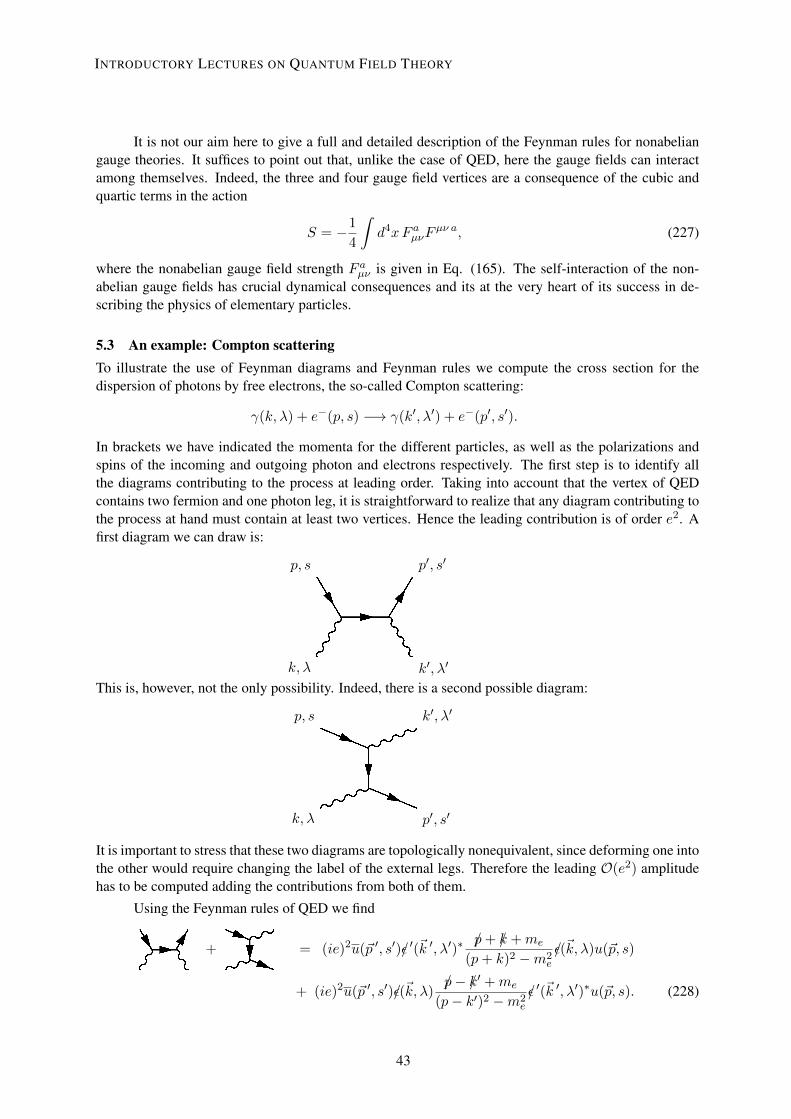
It is not our aim here to give a full and detailed description of the Feynman rules for nonabeliangauge theories. It suffices to point out that, unlike the case of QED, here the gauge fields can interactamong themselves. Indeed, the three and four gauge field vertices are a consequence of the cubic andquartic terms in the action

S = −1

4

∫d4xF a

µνFµν a, (227)

where the nonabelian gauge field strength F aµν is given in Eq. (165). The self-interaction of the non-

abelian gauge fields has crucial dynamical consequences and its at the very heart of its success in de-scribing the physics of elementary particles.

5.3 An example: Compton scatteringTo illustrate the use of Feynman diagrams and Feynman rules we compute the cross section for thedispersion of photons by free electrons, the so-called Compton scattering:

γ(k, λ) + e−(p, s) −→ γ(k′, λ′) + e−(p′, s′).

In brackets we have indicated the momenta for the different particles, as well as the polarizations andspins of the incoming and outgoing photon and electrons respectively. The first step is to identify allthe diagrams contributing to the process at leading order. Taking into account that the vertex of QEDcontains two fermion and one photon leg, it is straightforward to realize that any diagram contributing tothe process at hand must contain at least two vertices. Hence the leading contribution is of order e2. Afirst diagram we can draw is:

k, λ

p, s

k′, λ′

p′, s′

This is, however, not the only possibility. Indeed, there is a second possible diagram:

k, λ

p, s

p′, s′

k′, λ′

It is important to stress that these two diagrams are topologically nonequivalent, since deforming one intothe other would require changing the label of the external legs. Therefore the leading O(e2) amplitudehas to be computed adding the contributions from both of them.

Using the Feynman rules of QED we find

+ = (ie)2u(p ′, s′)/ϵ ′(k ′, λ′)∗ /p+ /k +me

(p+ k)2 −m2e

/ϵ(k, λ)u(p, s)

+ (ie)2u(p ′, s′)/ϵ(k, λ)/p− /k′ +me

(p− k′)2 −m2e

/ϵ ′(k ′, λ′)∗u(p, s). (228)

43


43

Because the leading order contributions only involve tree-level diagrams, there is no integration overinternal momenta and therefore we are left with a purely algebraic expression for the amplitude. To getan explicit expression we begin by simplifying the numerators. The following simple identity turns outto be very useful for this task

/a/b = −/b/a+ 2(a · b)1. (229)

Indeed, looking at the first term in Eq. (228) we have

(/p+ /k +me)/ϵ(k, λ)u(p, s) = −/ϵ(k, λ)(/p−me)u(p, s) + /k/ϵ(k, λ)u(p, s)

+ 2p · ϵ(k, λ)u(p, s), (230)

where we have applied the identity (229) on the first term inside the parenthesis. The first term onthe right-hand side of this equation vanishes identically because of Eq. (125). The expression can befurther simplified if we restrict our attention to the Compton scattering at low energy when electrons arenonrelativistic. This means that all spatial momenta are much smaller than the electron mass

|p|, |k|, |p ′|, |k ′| ≪ me. (231)

In this approximation we have that pµ, p′µ ≈ (me, 0) and therefore

p · ϵ(k, λ) = 0. (232)

This follows from the absence of temporal photon polarization. Then we conclude that at low energies

(/p+ /k +me)/ϵ(k, λ)u(p, s) = /k/ϵ(k, λ)u(p, s) (233)

and similarly for the second term in Eq. (228)

(/p− /k′ +me)/ϵ′(k′, λ′)∗u(p, s) = −/k′/ϵ ′(k′, λ′)∗u(p, s). (234)

Next, we turn to the denominators in Eq. (228). As it was explained in Section 5.2, in computingscattering amplitudes incoming and outgoing particles should have on-shell momenta,

p2 = m2e = p′2 and k2 = 0 = k′2. (235)

Then, the two denominator in Eq. (228) simplify respectively to

(p+ k)2 −m2e = p2 + k2 + 2p · k −m2

e = 2p · k = 2ωp |k| − 2p · k (236)

and

(p− k′)2 −m2e = p2 + k′2 + 2p · k′ −m2

e = −2p · k′ = −2ωp |k ′| + 2p · k ′. (237)

Working again in the low energy approximation (231) these two expressions simplify to

(p+ k)2 −m2e ≈ 2me |k|, (p− k′)2 −m2

e ≈ −2me |k ′|. (238)

Putting together all these expressions we find that at low energies

+≈ (ie)2

2meu(p ′, s′)

[/ϵ ′(k ′λ′)∗ /k

|k|ϵ(k, λ) + ϵ(k, λ)

/k′

|k ′|/ϵ ′(k ′λ′)∗

]u(p, s). (239)

44


44

Using now again the identity (229) a number of times as well as the transversality condition of thepolarization vectors (156) we end up with a handier equation + ≈ e2

me

[ϵ(k, λ) · ϵ′(k ′, λ′)∗

]u(p ′, s′)

/k

|k|u(p, s)

+e2

2meu(p ′, s′)/ϵ(k, λ)/ϵ ′(k ′, λ′)∗

(/k

|k|− /k′

|k ′|

)u(p, s). (240)

With a little bit of effort we can show that the second term on the right-hand side vanishes. First wenotice that in the low energy limit |k| ≈ |k ′|. If in addition we make use the conservation of momentumk − k ′ = p ′ − p and the identity (125)

u(p ′, s′)/ϵ(k, λ)/ϵ ′(k ′, λ′)∗(/k

|k|− /k′

|k ′|

)u(p, s)

≈ 1

|k|u(p ′, s′)/ϵ(k, λ)/ϵ ′(k ′, λ′)∗(/p′ −me)u(p, s). (241)

Next we use the identity (229) to take the term (/p′ −me) to the right. Taking into account that in the lowenergy limit the electron four-momenta are orthogonal to the photon polarization vectors [see Eq. (232)]we conclude that

u(p ′, s′)/ϵ(k, λ)/ϵ ′(k ′, λ′)∗(/p′ −me)u(p, s)

= u(p ′, s′)(/p′ −me)/ϵ(k, λ)/ϵ ′(k ′, λ′)∗u(p, s) = 0 (242)

where the last identity follows from the equation satisfied by the conjugate positive-energy spinor,u(p ′, s′)(/p′ −me) = 0.

After all these lengthy manipulations we have finally arrived at the expression of the invariantamplitude for the Compton scattering at low energies

iM =e2

me

[ϵ(k, λ) · ϵ′(k ′, λ′)∗

]u(p ′, s′)

/k

|k|u(p, s). (243)

The calculation of the cross section involves computing the modulus squared of this quantity. For manyphysical applications, however, one is interested in the dispersion of photons with a given polarizationby electrons that are not polarized, i.e. whose spins are randomly distributed. In addition in manysituations either we are not interested, or there is no way to measure the final polarization of the outgoingelectron. This is for example the situation in cosmology, where we do not have any information aboutthe polarization of the free electrons in the primordial plasma before or after the scattering with photons(although we have ways to measure the polarization of the scattered photons).

To describe this physical situations we have to average over initial electron polarization (since wedo not know them) and sum over all possible final electron polarization (because our detector is blind tothis quantum number),

|iM|2 =1

2

(e2

me |k|

)2 ∣∣∣ϵ(k, λ) · ϵ′(k ′, λ′)∗∣∣∣2 ∑

s=± 12

∑

s′=± 12

∣∣∣u(p ′, s′)/ku(p, s)∣∣∣2. (244)

The factor of 12 comes from averaging over the two possible polarizations of the incoming electrons.

The sums in this expression can be calculated without much difficulty. Expanding the absolute valueexplicitly

∑

s=± 12

∑

s′=± 12

∣∣∣u(p ′, s′)/ku(p, s)∣∣∣2

=∑

s=± 12

∑

s′=± 12

[u(p, s)†/k†u(p ′, s′)†

][u(p ′, s′)/ku(p, s)

], (245)

45


45

using that γµ† = γ0γµγ0 and after some manipulation one finds that

∑

s=± 12

∑

s′=± 12

∣∣∣u(p ′, s′)/ku(p, s)∣∣∣2

=

∑

s=± 12

uα(p, s)uβ(p, s)

(/k)βσ

∑

s′=± 12

uσ(p ′, s′)uρ(p′, s′)

(/k)ρα

= Tr[(/p+me)/k(/p

′ +me)/k], (246)

where the final expression has been computed using the completeness relations in Eq. (128). The finalevaluation of the trace can be done using the standard Dirac matrices identities. Here we compute itapplying again the relation (229) to commute /p′ and /k. Using that k2 = 0 and that we are working in thelow energy limit we have12

Tr[(/p+me)/k(/p

′ +me)/k]

= 2(p · k)(p′ · k)Tr1 ≈ 8m2e |k|2. (247)

This gives the following value for the invariant amplitude

|iM|2 = 4e4∣∣∣ϵ(k, λ) · ϵ′(k ′, λ′)∗

∣∣∣2

(248)

Plugging |iM|2 into the formula for the differential cross section we get

dσ

dΩ=

1

64π2m2e

|iM|2 =

(e2

4πme

)2 ∣∣∣ϵ(k, λ) · ϵ′(k ′, λ′)∗∣∣∣2. (249)

The prefactor of the last equation is precisely the square of the so-called classical electron radius rcl. Infact, the previous differential cross section can be rewritten as

dσ

dΩ=

3

8πσT

∣∣∣ϵ(k, λ) · ϵ′(k ′, λ′)∗∣∣∣2, (250)

where σT is the total Thomson cross section

σT =e4

6πm2e

=8π

3r2cl. (251)

The result (250) is relevant in many areas of Physics, but its importance is paramount in the studyof the cosmological microwave background (CMB). Just before recombination the universe is filled bya plasma of electrons interacting with photons via Compton scattering, with temperatures of the order of1 keV. Electrons are then nonrelativistic (me ∼ 0.5 MeV) and the approximations leading to Eq. (250)are fully valid. Because we do not know the polarization state of the photons before being scattered byelectrons we have to consider the cross section averaged over incoming photon polarizations. From Eq.(250) we see that this is proportional to

1

2

∑

λ=1,2

∣∣∣ϵ(k, λ) · ϵ′(k ′, λ′)∗∣∣∣2

=

1

2

∑

λ=1,2

ϵi(k, λ)ϵj(k, λ)∗

ϵj(k ′, λ′)ϵi(k ′, λ′)∗. (252)

The sum inside the brackets can be computed using the normalization of the polarization vectors, |ϵ (k, λ)|2 =1, and the transversality condition k · ϵ(k, λ) = 0

1

2

∑

λ=1,2

∣∣∣ϵ(k, λ) · ϵ′(k ′, λ′)∗∣∣∣2

=1

2

(δij − kikj

|k|2

)ϵ′j(k

′, λ′)ϵ′i(k′, λ′)∗

12We use also the fact that the trace of the product of an odd number of Dirac matrices is always zero.

46


46

=1

2

[1 − |ℓ · ϵ ′(k ′, λ′)|2

], (253)

where ℓ = k

|k| is the unit vector in the direction of the incoming photon.

From the last equation we conclude that Thomson scattering suppresses all polarizations parallel tothe direction of the incoming photon ℓ, whereas the differential cross section reaches the maximum in theplane normal to ℓ. If photons would collide with the electrons in the plasma with the same intensity fromall directions, the result would be an unpolarized CMB radiation. The fact that polarization is actuallymeasured in the CMB carries crucial information about the physics of the plasma before recombinationand, as a consequence, about the very early universe (see for example [22] for a throughout discussion).

6 Symmetries6.1 Noether’s theoremIn Classical Mechanics and Classical Field Theory there is a basic result that relates symmetries andconserved charges. This is called Noether’s theorem and states that for each continuous symmetry of thesystem there is conserved current. In its simplest version in Classical Mechanics it can be easily proved.Let us consider a Lagrangian L(qi, qi) which is invariant under a transformation qi(t) → q′

i(t, ϵ) labelledby a parameter ϵ. This means that L(q′, q′) = L(q, q) without using the equations of motion13. If ϵ ≪ 1we can consider an infinitesimal variation of the coordinates δϵqi(t) and the invariance of the Lagrangianimplies

0 = δϵL(qi, qi) =∂L

∂qiδϵqi +

∂L

∂qiδϵqi =

[∂L

∂qi− d

dt

∂L

∂qi

]δϵqi +

d

dt

(∂L

∂qiδϵqi

). (254)

When δϵqi is applied on a solution to the equations of motion the term inside the square brackets vanishesand we conclude that there is a conserved quantity

Q = 0 with Q ≡ ∂L

∂qiδϵqi. (255)

Notice that in this derivation it is crucial that the symmetry depends on a continuous parameter sinceotherwise the infinitesimal variation of the Lagrangian in Eq. (254) does not make sense.

In Classical Field Theory a similar result holds. Let us consider for simplicity a theory of a singlefield ϕ(x). We say that the variations δϵϕ depending on a continuous parameter ϵ are a symmetry of thetheory if, without using the equations of motion, the Lagrangian density changes by

δϵL = ∂µKµ. (256)

If this happens then the action remains invariant and so do the equations of motion. Working out now thevariation of L under δϵϕ we find

∂µKµ =

∂L∂(∂µϕ)

∂µδϵϕ+∂L∂ϕ

δϵϕ = ∂µ

(∂L

∂(∂µϕ)δϵϕ

)+

[∂L∂ϕ

− ∂µ

(∂L

∂(∂µϕ)

)]δϵϕ. (257)

If ϕ(x) is a solution to the equations of motion the last terms disappears, and we find that there is aconserved current

∂µJµ = 0 with Jµ =

∂L∂(∂µϕ)

δϵϕ−Kµ. (258)

13The following result can be also derived a more general situations where the Lagrangian changes by a total time derivative.

47


47

Actually a conserved current implies the existence of a charge

Q ≡∫d3xJ0(t, x) (259)

which is conserved

dQ

dt=

∫d3x ∂0J

0(t, x) = −∫d3x ∂iJ

i(t, x) = 0, (260)

provided the fields vanish at infinity fast enough. Moreover, the conserved charge Q is a Lorentz scalar.After canonical quantization the charge Q defined by Eq. (259) is promoted to an operator that generatesthe symmetry on the fields

δϕ = i[ϕ,Q]. (261)

As an example we can consider a scalar field ϕ(x) which under a coordinate transformation x → x′

changes as ϕ′(x′) = ϕ(x). In particular performing a space-time translation xµ ′= xµ + aµ we have

ϕ′(x) − ϕ(x) = −aµ∂µϕ+ O(a2) =⇒ δϕ = −aµ∂µϕ. (262)

Since the Lagrangian density is also a scalar quantity, it transforms under translations as

δL = −aµ∂µL. (263)

Therefore the corresponding conserved charge is

Jµ = − ∂L∂(∂µϕ)

aν∂νϕ+ aµL ≡ −aνTµν , (264)

where we introduced the energy-momentum tensor

Tµν =∂L

∂(∂µϕ)∂νϕ− ηµνL. (265)

We find that associated with the invariance of the theory with respect to space-time translations thereare four conserved currents defined by Tµν with ν = 0, . . . , 3, each one associated with the translationalong a space-time direction. These four currents form a rank-two tensor under Lorentz transformationssatisfying

∂µTµν = 0. (266)

The associated conserved charges are given by

P ν =

∫d3xT 0ν (267)

and correspond to the total energy-momentum content of the field configuration. Therefore the energydensity of the field is given by T 00 while T 0i is the momentum density. In the quantum theory the Pµ

are the generators of space-time translations.

Another example of a symmetry related with a physically relevant conserved charge is the globalphase invariance of the Dirac Lagrangian (117), ψ → eiθψ. For small θ this corresponds to variationsδθψ = iθψ, δθψ = −iθψ which by Noether’s theorem result in the conserved charge

jµ = ψγµψ, ∂µjµ = 0. (268)

48


48

Thus implying the existence of a conserved charge

Q =

∫d3xψγ0ψ =

∫d3xψ†ψ. (269)

In physics there are several instances of global U(1) symmetries that act as phase shifts on spinors.This is the case, for example, of the baryon and lepton number conservation in the Standard Model. Amore familiar case is the U(1) local symmetry associated with electromagnetism. Notice that althoughin this case we are dealing with a local symmetry, θ → eα(x), the invariance of the Lagrangian holdsin particular for global transformations and therefore there is a conserved current jµ = eψγµψ. InEq. (162) we saw that the spinor is coupled to the photon field precisely through this current. Its timecomponent is the electric charge density ρ, while the spatial components are the current density vector ȷ.

This analysis can be carried over also to nonabelian unitary global symmetries acting as

ψi −→ Uijψj , U †U = 1 (270)

and leaving invariant the Dirac Lagrangian when we have several fermions. If we write the matrix U interms of the hermitian group generators T a as

U = exp (iαaTa) , (T a)† = T a, (271)

we find the conserved current

jµ a = ψiTaijγ

µψj , ∂µjµ = 0. (272)

This is the case, for example of the approximate flavor symmetries in hadron physics. The simplestexample is the isospin symmetry that mixes the quarks u and d

(ud

)−→ M

(ud

), M ∈ SU(2). (273)

Since the proton is a bound state of two quarks u and one quark d while the neutron is made out ofone quark u and two quarks d, this isospin symmetry reduces at low energies to the well known isospintransformations of nuclear physics that mixes protons and neutrons.

6.2 Symmetries in the quantum theoryWe have seen that in canonical quantization the conserved charges Qa associated to symmetries byNoether’s theorem are operators implementing the symmetry at the quantum level. Since the charges areconserved they must commute with the Hamiltonian

[Qa,H] = 0. (274)

There are several possibilities in the quantum mechanical realization of a symmetry:

Wigner-Weyl realization. In this case the ground state of the theory |0⟩ is invariant under thesymmetry. Since the symmetry is generated by Qa this means that

U(α)|0⟩ ≡ eiαaQa |0⟩ = |0⟩ =⇒ Qa|0⟩ = 0. (275)

At the same time the fields of the theory have to transform according to some irreducible representationof the group generated by the Qa. From Eq. (261) it is easy to prove that

U(α)ϕiU(α)−1 = Uij(α)ϕj , (276)

49


49

where Uij(α) is an element of the representation in which the field ϕi transforms. If we consider nowthe quantum state associated with the operator ϕi

|i⟩ = ϕi|0⟩ (277)

we find that because of the invariance of the vacuum (275) the states |i⟩ transform in the same represen-tation as ϕi

U(α)|i⟩ = U(α)ϕiU(α)−1U(α)|0⟩ = Uij(α)ϕj |0⟩ = Uij(α)|j⟩. (278)

Therefore the spectrum of the theory is classified in multiplets of the symmetry group. In addition, since[H,U(α)] = 0 all states in the same multiplet have the same energy. If we consider one-particle states,then going to the rest frame we conclude that all states in the same multiplet have exactly the same mass.

Nambu-Goldstone realization. In our previous discussion the result that the spectrum of thetheory is classified according to multiplets of the symmetry group depended crucially on the invarianceof the ground state. However this condition is not mandatory and one can relax it to consider theorieswhere the vacuum state is not left invariant by the symmetry

eiαaQa |0⟩ = |0⟩ =⇒ Qa|0⟩ = 0. (279)

In this case it is also said that the symmetry is spontaneously broken by the vacuum.

To illustrate the consequences of (279) we consider the example of a number scalar fields φi

(i = 1, . . . , N ) whose dynamics is governed by the Lagrangian

L =1

2∂µφ

i∂µφi − V (φ), (280)

where we assume that V (ϕ) is bounded from below. This theory is globally invariant under the transfor-mations

δφi = ϵa(T a)ijφ

j , (281)

with T a, a = 1, . . . , 12N(N − 1) the generators of the group SO(N).

To analyze the structure of vacua of the theory we construct the Hamiltonian

H =

∫d3x

[1

2πiπi +

1

2∇φi · ∇φi + V (φ)

](282)

and look for the minimum of

V(φ) =

∫d3x

[1

2∇φi · ∇φi + V (φ)

]. (283)

Since we are interested in finding constant field configurations, ∇φ = 0 to preserve translational invari-ance, the vacua of the potential V(φ) coincides with the vacua of V (φ). Therefore the minima of thepotential correspond to the vacuum expectation values14

⟨φi⟩ : V (⟨φi⟩) = 0,∂V

∂φi

∣∣∣∣φi=⟨φi⟩

= 0. (284)

We divide the generators T a of SO(N ) into two groups: Those denoted by Hα (α = 1, . . . , h)that satisfy

(Hα)ij⟨φj⟩ = 0. (285)

14For simplicity we consider that the minima of V (ϕ) occur at zero potential.

50


50

This means that the vacuum configuration ⟨φi⟩ is left invariant by the transformation generated by Hα.For this reason we call them unbroken generators. Notice that the commutator of two unbroken genera-tors also annihilates the vacuum expectation value, [Hα,Hβ]ij⟨φj⟩ = 0. Therefore the generators Hαform a subalgebra of the algebra of the generators of SO(N ). The subgroup of the symmetry groupgenerated by them is realized à la Wigner-Weyl.

The remaining generators KA, with A = 1, . . . , 12N(N − 1) − h, by definition do not preserve

the vacuum expectation value of the field

(KA)ij⟨φj⟩ = 0. (286)

These will be called the broken generators. Next we prove a very important result concerning the brokengenerators known as the Goldstone theorem: for each generator broken by the vacuum expectation valuethere is a massless excitation.

The mass matrix of the excitations around the vacuum ⟨φi⟩ is determined by the quadratic part ofthe potential. Since we assumed that V (⟨φ⟩) = 0 and we are expanding around a minimum, the firstterm in the expansion of the potential V (φ) around the vacuum expectation values is given by

V (φ) =∂2V

∂φi∂φj

∣∣∣∣φ=⟨φ⟩

(φi − ⟨φi⟩)(φj − ⟨φj⟩) + O[(φ− ⟨φ⟩)3

](287)

and the mass matrix is:

M2ij ≡ ∂2V

∂φi∂φj

∣∣∣∣φ=⟨φ⟩

. (288)

In order to avoid a cumbersome notation we do not show explicitly the dependence of the mass matrixon the vacuum expectation values ⟨φi⟩.

To extract some information about the possible zero modes of the mass matrix, we write down theconditions that follow from the invariance of the potential under δφi = ϵa(T a)i

jφj . At first order in ϵa

δV (φ) = ϵa∂V

∂φi(T a)i

jφj = 0. (289)

Differentiating this expression with respect to φk we arrive at

∂2V

∂φi∂φk(T a)i

jφj +

∂V

∂φi(T a)i

k = 0. (290)

Now we evaluate this expression in the vacuum φi = ⟨φi⟩. Then the derivative in the second term cancelswhile the second derivative in the first one gives the mass matrix. Hence we find

M2ik(T

a)ij⟨φj⟩ = 0. (291)

Now we can write this expression for both broken and unbroken generators. For the unbroken ones, since(Hα)i

j⟨φj⟩ = 0, we find a trivial identity 0 = 0. On the other hand for the broken generators we have

M2ik(K

A)ij⟨φj⟩ = 0. (292)

Since (KA)ij⟨φj⟩ = 0 this equation implies that the mass matrix has as many zero modes as broken

generators. Therefore we have proven Goldstone’s theorem: associated with each broken symmetrythere is a massless mode in the theory. Here we have presented a classical proof of the theorem. In thequantum theory the proof follows the same lines as the one presented here but one has to consider theeffective action containing the effects of the quantum corrections to the classical Lagrangian.

51


51

As an example to illustrate this theorem, we consider a SO(3) invariant scalar field theory with a“mexican hat” potential

V (φ) =λ

4

(φ 2 − a2

)2. (293)

The vacua of the theory correspond to the configurations satisfying ⟨φ⟩ 2 = a2. In field space this equa-tion describes a two-dimensional sphere and each solution is just a point in that sphere. Geometricallyit is easy to visualize that a given vacuum field configuration, i.e. a point in the sphere, is preservedby SO(2) rotations around the axis of the sphere that passes through that point. Hence the vacuumexpectation value of the scalar field breaks the symmetry according to

⟨φ⟩ : SO(3) −→ SO(2). (294)

Since SO(3) has three generators and SO(2) only one we see that two generators are broken and there-fore there are two massless Goldstone bosons. Physically this massless modes can be thought of ascorresponding to excitations along the surface of the sphere ⟨φ⟩ 2 = a2.

Once a minimum of the potential has been chosen we can proceed to quantize the excitationsaround it. Since the vacuum only leaves invariant a SO(2) subgroup of the original SO(3) symmetrygroup it seems that the fact that we are expanding around a particular vacuum expectation value of thescalar field has resulted in a lost of symmetry. This is however not the case. The full quantum theoryis symmetric under the whole symmetry group SO(3). This is reflected in the fact that the physicalproperties of the theory do not depend on the particular point of the sphere ⟨φ⟩ 2 = a2 that we havechosen. Different vacua are related by the full SO(3) symmetry and therefore should give the samephysics.

It is very important to realize that given a theory with a vacuum determined by ⟨φ⟩ all otherpossible vacua of the theory are unaccessible in the infinite volume limit. This means that two vacuumstates |01⟩, |02⟩ corresponding to different vacuum expectation values of the scalar field are orthogonal⟨01|02⟩ = 0 and cannot be connected by any local observable Φ(x), ⟨01|Φ(x)|02⟩ = 0. Heuristicallythis can be understood by noticing that in the infinite volume limit switching from one vacuum intoanother one requires changing the vacuum expectation value of the field everywhere in space at the sametime, something that cannot be done by any local operator. Notice that this is radically different to ourexpectations based on the Quantum Mechanics of a system with a finite number of degrees of freedom.

In High Energy Physics the typical example of a Goldstone boson is the pion, associated withthe spontaneous breaking of the global chiral isospin SU(2)L × SU(2)R symmetry. This symmetry actsindependently in the left- and right-handed spinors as

(uL,R

dL,R

)−→ ML,R

(uL,R

dL,R

), ML,R ∈ SU(2)L,R (295)

Presumably since the quarks are confined at low energies this symmetry is spontaneously broken downto the diagonal SU(2) acting in the same way on the left- and right-handed components of the spinors.Associated with this symmetry breaking there is a Goldstone mode which is identified as the pion. No-tice, nevertheless, that the SU(2)L×SU(2)R would be an exact global symmetry of the QCD Lagrangianonly in the limit when the masses of the quarks are zero mu,md → 0. Since these quarks have nonzeromasses the chiral symmetry is only approximate and as a consequence the corresponding Goldstone bo-son is not massless. That is why pions have masses, although they are the lightest particle among thehadrons.

Symmetry breaking appears also in many places in condensed matter. For example, when a solidcrystallizes from a liquid the translational invariance that is present in the liquid phase is broken to adiscrete group of translations that represent the crystal lattice. This symmetry breaking has Goldstone

52


52

bosons associated which are identified with phonons which are the quantum excitation modes of thevibrational degrees of freedom of the lattice.

The Higgs mechanism. Gauge symmetry seems to prevent a vector field from having a mass.This is obvious once we realize that a term in the Lagrangian like m2AµA

µ is incompatible with gaugeinvariance.

However certain physical situations seem to require massive vector fields. This happened forexample during the 1960s in the study of weak interactions. The Glashow model gave a common de-scription of both electromagnetic and weak interactions based on a gauge theory with group SU(2)×U(1)but, in order to reproduce Fermi’s four-fermion theory of the β-decay it was necessary that two of thevector fields involved would be massive. Also in condensed matter physics massive vector fields arerequired to describe certain systems, most notably in superconductivity.

The way out to this situation is found in the concept of spontaneous symmetry breaking discussedpreviously. The consistency of the quantum theory requires gauge invariance, but this invariance can berealized à la Nambu-Goldstone. When this is the case the full gauge symmetry is not explicitly present inthe effective action constructed around the particular vacuum chosen by the theory. This makes possiblethe existence of mass terms for gauge fields without jeopardizing the consistency of the full theory, whichis still invariant under the whole gauge group.

To illustrate the Higgs mechanism we study the simplest example, the Abelian Higgs model: aU(1) gauge field coupled to a self-interacting charged complex scalar field Φ with Lagrangian

L = −1

4FµνF

µν +DµΦDµΦ − λ

4

(ΦΦ − µ2

)2, (296)

where the covariant derivative is given by Eq. (159). This theory is invariant under the gauge transfor-mations

Φ → eiα(x)Φ, Aµ → Aµ + ∂µα(x). (297)

The minimum of the potential is defined by the equation |Φ| = µ. We have a continuum of differentvacua labelled by the phase of the scalar field. None of these vacua, however, is invariant under thegauge symmetry

⟨Φ⟩ = µeiϑ0 → µeiϑ0+iα(x) (298)

and therefore the symmetry is spontaneously broken Let us study now the theory around one of thesevacua, for example ⟨Φ⟩ = µ, by writing the field Φ in terms of the excitations around this particularvacuum

Φ(x) =

[µ+

1√2σ(x)

]eiϑ(x). (299)

Independently of whether we are expanding around a particular vacuum for the scalar field we shouldkeep in mind that the whole Lagrangian is still gauge invariant under (297). This means that perform-ing a gauge transformation with parameter α(x) = −ϑ(x) we can get rid of the phase in Eq. (299).Substituting then Φ(x) = µ+ 1√

2σ(x) in the Lagrangian we find

L = −1

4FµνF

µν + e2µ2AµAµ +

1

2∂µσ∂

µσ − 1

2λµ2σ2

− λµσ3 − λ

4σ4 + e2µAµA

µσ + e2AµAµσ2. (300)

What are the excitation of the theory around the vacuum ⟨Φ⟩ = µ? First we find a massive real scalarfield σ(x). The important point however is that the vector field Aµ now has a mass given by

m2γ = 2e2µ2. (301)

53


53

The remarkable thing about this way of giving a mass to the photon is that at no point we have given upgauge invariance. The symmetry is only hidden. Therefore in quantizing the theory we can still enjoy allthe advantages of having a gauge theory but at the same time we have managed to generate a mass forthe gauge field.

It is surprising, however, that in the Lagrangian (300) we did not find any massless mode. Since thevacuum chosen by the scalar field breaks theU(1) generator of U(1) we would have expected one maslessparticle from Goldstone’s theorem. To understand the fate of the missing Goldstone boson we have torevisit the calculation leading to Eq. (300). Were we dealing with a global U(1) theory, the Goldstoneboson would correspond to excitation of the scalar field along the valley of the potential and the phaseϑ(x) would be the massless Goldstone boson. However we have to keep in mind that in computing theLagrangian we managed to get rid of ϑ(x) by shifting it into Aµ using a gauge transformation. Actuallyby identifying the gauge parameter with the Goldstone excitation we have completely fixed the gaugeand the Lagrangian (300) does not have any gauge symmetry left.

A massive vector field has three polarizations: two transverse ones k · ϵ (k,±1) = 0 plus a longi-tudinal one ϵL(k) ∼ k. In gauging away the massless Goldstone boson ϑ(x) we have transformed it intothe longitudinal polarization of the massive vector field. In the literature this is usually expressed sayingthat the Goldstone mode is “eaten up” by the longitudinal component of the gauge field. It is importantto realize that in spite of the fact that the Lagrangian (300) looks pretty different from the one we startedwith we have not lost any degrees of freedom. We started with the two polarizations of the photon plusthe two degrees of freedom associated with the real and imaginary components of the complex scalarfield. After symmetry breaking we end up with the three polarizations of the massive vector field and thedegree of freedom of the real scalar field σ(x).

We can also understand the Higgs mechanism in the light of our discussion of gauge symmetryin section 4.4. In the Higgs mechanism the invariance of the theory under infinitesimal gauge trans-formations is not explicitly broken, and this implies that Gauss’ law is satisfied quantum mechanically,∇ · Ea|phys⟩ = 0. The theory remains invariant under gauge transformations in the connected com-ponent of the identity G0, the ones generated by Gauss’ law. This does not pose any restriction on thepossible breaking of the invariance of the theory with respect to transformations that cannot be continu-ously deformed to the identity. Hence in the Higgs mechanism the invariance under gauge transformationthat are not in the connected component of the identity, G/G0, can be broken. Let us try to put it in moreprecise terms. As we learned in section 4.4, in the Hamiltonian formulation of the theory finite energygauge field configurations tend to a pure gauge at spatial infinity

Aµ(x)−→ − 1

igg(x)∇g(x)−1, |x| → ∞ (302)

The set transformations g0(x) ∈ G0 that tend to the identity at infinity are the ones generated by Gauss’law. However, one can also consider in general gauge transformations g(x) which, as |x| → ∞, approachany other element g ∈ G. The quotient G∞ ≡ G/G0 gives a copy of the gauge group at infinity. Thereis no reason, however, why this group should not be broken, and in general it is if the gauge symmetryis spontaneously broken. Notice that this is not a threat to the consistency of the theory. Propertieslike the decoupling of unphysical states are guaranteed by the fact that Gauss’ law is satisfied quantummechanically and are not affected by the breaking of G∞.

The Abelian Higgs model discussed here can be regarded as a toy model of the Higgs mechanismresponsible for giving mass to theW± and Z0 gauge bosons in the Standard Model. In condensed matterphysics the symmetry breaking described by the nonrelativistic version of the Abelian Higgs model canbe used to characterize the onset of a superconducting phase in the BCS theory, where the complex scalarfield Φ is associated with the Cooper pairs. In this case the parameter µ2 depends on the temperature.Above the critical temperature Tc, µ2(T ) > 0 and there is only a symmetric vacuum ⟨Φ⟩ = 0. When,on the other hand, T < Tc then µ2(T ) < 0 and symmetry breaking takes place. The onset of a nonzero

54


54

mass of the photon (301) below the critical temperature explains the Meissner effect: the magnetic fieldscannot penetrate inside superconductors beyond a distance of the order 1

mγ.

7 AnomaliesSo far we did not worry too much about how classical symmetries of a theory are carried over to thequantum theory. We have implicitly assumed that classical symmetries are preserved in the process ofquantization, so they are also realized in the quantum theory.

This, however, does not have to be necessarily the case. Quantizing an interacting field theoryis a very involved process that requires regularization and renormalization and sometimes, it does notmatter how hard we try, there is no way for a classical symmetry to survive quantization. When thishappens one says that the theory has an anomaly (for a review see [28]). It is important to avoid here themisconception that anomalies appear due to a bad choice of the way a theory is regularized in the processof quantization. When we talk about anomalies we mean a classical symmetry that cannot be realized inthe quantum theory, no matter how smart we are in choosing the regularization procedure.

In the following we analyze some examples of anomalies associated with global and local sym-metries of the classical theory. In Section 8 we will encounter yet another example of an anomaly, thistime associated with the breaking of classical scale invariance in the quantum theory.

7.1 Axial anomalyProbably the best known examples of anomalies appear when we consider axial symmetries. If weconsider a theory of two Weyl spinors u±

L = iψ∂/ψ = iu†+σ

µ+∂µu+ + iu†

−σµ−∂µu− with ψ =

(u+

u−

)(303)

the Lagrangian is invariant under two types of global U(1) transformations. In the first one both helicitiestransform with the same phase, this is a vector transformation:

U(1)V : u± −→ eiαu±, (304)

whereas in the second one, the axial U(1), the signs of the phases are different for the two chiralities

U(1)A : u± −→ e±iαu±. (305)

Using Noether’s theorem, there are two conserved currents, a vector current

JµV = ψγµψ = u†

+σµ+u+ + u†

−σµ−u− =⇒ ∂µJ

µV = 0 (306)

and an axial vector current

JµA = ψγµγ5ψ = u†

+σµ+u+ − u†

−σµ−u− =⇒ ∂µJ

µA = 0. (307)

The theory described by the Lagrangian (303) can be coupled to the electromagnetic field. Theresulting classical theory is still invariant under the vector and axial U(1) symmetries (304) and (305).Surprisingly, upon quantization it turns out that the conservation of the axial current (307) is spoiled byquantum effects

∂µJµA ∼ ℏ E · B. (308)

To understand more clearly how this result comes about we study first a simple model in twodimensions that captures the relevant physics involved in the four-dimensional case [29]. We work in

55


55

Minkowski space in two dimensions with coordinates (x0, x1) ≡ (t, x) and where the spatial directionis compactified to a circle S1. In this setup we consider a fermion coupled to the electromagnetic field.Notice that since we are living in two dimensions the field strength Fµν only has one independent com-ponent that corresponds to the electric field along the spatial direction, F 01 ≡ E (in two dimensions thereare no magnetic fields!).

To write the Lagrangian for the spinor field we need to find a representation of the algebra ofγ-matrices

γµ, γν = 2ηµν with η =

(1 00 −1

). (309)

In two dimensions the dimension of the representation of the γ-matrices is 2[ 22] = 2. Here take

γ0 ≡ σ1 =

(0 11 0

), γ1 ≡ iσ2 =

(0 1

−1 0

). (310)

This is a chiral representation since the matrix γ5 is diagonal15

γ5 ≡ −γ0γ1 =

(1 00 −1

)(311)

Writing the two-component spinor ψ as

ψ =

(u+

u−

)(312)

and defining as usual the projectors P± = 12(1±γ5) we find that the components u± of ψ are respectively

a right- and left-handed Weyl spinor in two dimensions.

Once we have a representation of the γ-matrices we can write the Dirac equation. Expressing it interms of the components u± of the Dirac spinor we find

(∂0 − ∂1)u+ = 0, (∂0 + ∂1)u− = 0. (313)

The general solution to these equations can be immediately written as

u+ = u+(x0 + x1), u− = u−(x0 − x1). (314)

Hence u± are two wave packets moving along the spatial dimension respectively to the left (u+) andto the right (u−). Notice that according to our convention the left-moving u+ is a right-handed spinor(positive helicity) whereas the right-moving u− is a left-handed spinor (negative helicity).

If we want to interpret (313) as the wave equation for two-dimensional Weyl spinors we have thefollowing wave functions for free particles with well defined momentum pµ = (E, p).

u(E)± (x0 ± x1) =

1√Le−iE(x0±x1) with p = ∓E. (315)

As it is always the case with the Dirac equation we have both positive and negative energy solutions. Foru+, since E = −p, we see that the solutions with positive energy are those with negative momentump < 0, whereas the negative energy solutions are plane waves with p > 0. For the left-handed spinor u−the situation is reversed. Besides, since the spatial direction is compact with length L the momentum pis quantized according to

p =2πn

L, n ∈ Z. (316)

56


56

+ −

p p

E E

v v

Fig. 11: Spectrum of the massless two-dimensional Dirac field.

p

E E

p

0,+ 0,−

Fig. 12: Vacuum of the theory.

The spectrum of the theory is represented in Fig. 11.

Once we have the spectrum of the theory the next step is to obtain the vacuum. As with the Diracequation in four dimensions we fill all the states with E ≤ 0 (Fig. 12). Exciting of a particle in the Diracsee produces a positive energy fermion plus a hole that is interpreted as an antiparticle. This gives us theclue on how to quantize the theory. In the expansion of the operator u± in terms of the modes (315) weassociate positive energy states with annihilation operators whereas the states with negative energy are

15In any even number of dimensions γ5 is defined to satisfy the conditions γ25 = 1 and γ5, γ

µ = 0.

57


57

associated with creation operators for the corresponding antiparticle

u±(x) =∑

E>0

[a±(E)v

(E)± (x) + b†±(E)v

(E)± (x)∗

]. (317)

The operator a±(E) acting on the vacuum |0,±⟩ annihilates a particle with positive energy E and mo-mentum ∓E. In the same way b†±(E) creates out of the vacuum an antiparticle with positive energy Eand spatial momentum ∓E. In the Dirac sea picture the operator b±(E)† is originally an annihilationoperator for a state of the sea with negative energy −E. As in the four-dimensional case the problem ofthe negative energy states is solved by interpreting annihilation operators for negative energy states ascreation operators for the corresponding antiparticle with positive energy (and vice versa). The operatorsappearing in the expansion of u± in Eq. (317) satisfy the usual algebra

aλ(E), a†λ′(E

′) = bλ(E), b†λ′(E′) = δE,E′δλλ′ , (318)

where we have introduced the label λ, λ′ = ±. Also, aλ(E), a†λ(E) anticommute with bλ′(E′), b†λ′(E′).

The Lagrangian of the theory

L = iu†+(∂0 + ∂1)u+ + iu†

−(∂0 − ∂1)u− (319)

is invariant under both U(1)V , Eq. (304), and U(1)A, Eq. (305). The associated Noether currents are inthis case

JµV =

(u†

+u+ + u†−u−

−u†+u+ + u†

−u−

), Jµ

A =

(u†

+u+ − u†−u−

−u†+u+ − u†

−u−

). (320)

The associated conserved charges are given, for the vector current by

QV =

∫ L

0dx1

(u†

+u+ + u†−u−

)(321)

and for the axial current

QA =

∫ L

0dx1

(u†

+u+ − u†−u−

). (322)

Using the orthonormality relations for the modes v(E)± (x)

∫ L

0dx1 v

(E)± (x) v

(E′)± (x) = δE,E′ (323)

we find for the conserved charges:

QV =∑

E>0

[a†

+(E)a+(E) − b†+(E)b+(E) + a†−(E)a−(E) − b†−(E)b−(E)

],

QA =∑

E>0

[a†

+(E)a+(E) − b†+(E)b+(E) − a†−(E)a−(E) + b†−(E)b−(E)

]. (324)

We see that QV counts the net number (particles minus antiparticles) of positive helicity states plus thenet number of states with negative helicity. The axial charge, on the other hand, counts the net number ofpositive helicity states minus the number of negative helicity ones. In the case of the vector current wehave subtracted a formally divergent vacuum contribution to the charge (the “charge of the Dirac sea”).

In the free theory there is of course no problem with the conservation of eitherQV orQA, since theoccupation numbers do not change. What we want to study is the effect of coupling the theory to electric

58


58

p

E

Fig. 13: Effect of the electric field.

field E . We work in the gauge A0 = 0. Instead of solving the problem exactly we are going to simulatethe electric field by adiabatically varying in a long time τ0 the vector potential A1 from zero value to−Eτ0. From our discussion in section 4.3 we know that the effect of the electromagnetic coupling in thetheory is a shift in the momentum according to

p −→ p− eA1, (325)

where e is the charge of the fermions. Since we assumed that the vector potential varies adiabatically,we can assume it to be approximately constant at each time.

Then, we have to understand what is the effect of (325) on the vacuum depicted in Fig. (12). Whatwe find is that the two branches move as shown in Fig. (13) resulting in some of the negative energystates of the v+ branch acquiring positive energy while the same number of the empty positive energystates of the other branch v− will become empty negative energy states. Physically this means that theexternal electric field E creates a number of particle-antiparticle pairs out of the vacuum. Denoting byN ∼ eE the number of such pairs created by the electric field per unit time, the final values of the chargesQV and QA are

QA(τ0) = (N − 0) + (0 −N) = 0,

QV (τ0) = (N − 0) − (0 −N) = 2N. (326)

Therefore we conclude that the coupling to the electric field produces a violation in the conservation ofthe axial charge per unit time given by ∆QA ∼ eE . This implies that

∂µJµA ∼ eℏE , (327)

where we have restored ℏ to make clear that the violation in the conservation of the axial current is aquantum effect. At the same time ∆QV = 0 guarantees that the vector current remains conserved alsoquantum mechanically, ∂µJ

µV = 0.

59


59

We have just studied a two-dimensional example of the Adler-Bell-Jackiw axial anomaly [30].The heuristic analysis presented here can be made more precise by computing the quantity

Cµν = ⟨0|T[Jµ

A(x)JνV (0)

]|0⟩ =Jµ

Aγ

(328)

The anomaly is given then by ∂µCµν . A careful calculation yields the numerical prefactor missing in Eq.

(327) leading to the result

∂µJµA =

eℏ2πενσFνσ, (329)

with ε01 = −ε10 = 1.

The existence of an anomaly in the axial symmetry that we have illustrated in two dimensions ispresent in all even dimensional of space-times. In particular in four dimensions the axial anomaly it isgiven by

∂µJµA = − e2

16π2εµνσλFµνFσλ. (330)

This result has very important consequences in the physics of strong interactions as we will see in whatfollows

7.2 Chiral symmetry in QCDOur knowledge of the physics of strong interactions is based on the theory of Quantum Chromodynamics(QCD) [32]. This is a nonabelian gauge theory with gauge group SU(Nc) coupled to a number Nf ofquarks. These are spin-1

2 particlesQi f labelled by two quantum numbers: color i = 1, . . . , Nc and flavorf = 1, . . . , Nf . The interaction between them is mediated by the N2

c − 1 gauge bosons, the gluons Aaµ,

a = 1, . . . , N2c − 1. In the real world Nc = 3 and the number of flavors is six, corresponding to the

number of different quarks: up (u), down (d), charm (c), strange (s), top (t) and bottom (b).

For the time being we are going to study a general theory of QCD with Nc colors and Nf flavors.Also, for reasons that will be clear later we are going to work in the limit of vanishing quark masses,mf → 0. In this cases the Lagrangian is given by

LQCD = −1

4F a

µνFa µν +

Nf∑

f=1

[iQ

fLD/ Q

fL + iQ

fRD/ Q

fR

], (331)

where the subscripts L andR indicate respectively left and right-handed spinors,QfL,R ≡ P±Qf , and the

field strength F aµν and the covariant derivativeDµ are respectively defined in Eqs. (165) and (168). Apart

from the gauge symmetry, this Lagrangian is also invariant under a global U(Nf )L×U(Nf )R acting onthe flavor indices and defined by

U(Nf )L :

QfL → ∑

f ′(UL)ff ′Qf ′L

QfR → Qf

R

U(Nf )R :

QfL → Qf

L

QrR → ∑

f ′(UR)ff ′Qf ′R

(332)

60


60

with UL, UR ∈ U(Nf ). Actually, since U(N )=U(1)×SU(N ) this global symmetry group can be writtenas SU(Nf )L×SU(Nf )R×U(1)L×U(1)R. The abelian subgroup U(1)L×U(1)R can be now decomposedinto their vector U(1)B and axial U(1)A subgroups defined by the transformations

U(1)B :

QfL → eiαQf

L

QfR → eiαQf

R

U(1)A :

QfL → eiαQf

L

QfR → e−iαQf

R

(333)

According to Noether’s theorem, associated with these two abelian symmetries we have two conservedcurrents:

JµV =

Nf∑

f=1

QfγµQf , Jµ

A =

Nf∑

f=1

Qfγµγ5Q

f . (334)

The conserved charge associated with vector charge JµV is actually the baryon number defined as the

number of quarks minus number of antiquarks.

The nonabelian part of the global symmetry group SU(Nf )L×SU(Nf )R can also be decomposedinto its vector and axial subgroups, SU(Nf )V × SU(Nf )A, defined by the following transformations ofthe quarks fields

SU(Nf )V :

QfL → ∑


QfR → ∑

f ′(UL)ff ′Qf ′R

SU(Nf )A :

QfL → ∑


QfR → ∑

f ′(U−1R )ff ′Qf ′

R

(335)

Again, the application of Noether’s theorem shows the existence of the following nonabelian conservedcharges

JI µV ≡

Nf∑

f,f ′=1

Qfγµ(T I)ff ′Qf ′

, JI µA ≡

Nf∑

f,f ′=1

Qfγµγ5(T

I)ff ′Qf ′. (336)

To summarize, we have shown that the initial chiral symmetry of the QCD Lagrangian (331) can bedecomposed into its chiral and vector subgroups according to

U(Nf )L × U(Nf )R = SU(Nf )V × SU(Nf )A × U(1)B × U(1)A. (337)

The question to address now is which part of the classical global symmetry is preserved by the quantumtheory.

As argued in section 7.1, the conservation of the axial currents JµA and Ja µ

A can in principle bespoiled due to the presence of an anomaly. In the case of the abelian axial current Jµ

A the relevant quantityis the correlation function

Cµνσ ≡ ⟨0|T[Jµ

A(x)ja νgauge(x

′)jb σgauge(0)

]|0⟩ =

Nf∑

f=1

Jµ

A

Qf

g

Qf

g

Qf

symmetric

(338)

Here ja µgauge is the nonabelian conserved current coupling to the gluon field

ja µgauge ≡

Nf∑

f=1

QfγµτaQf , (339)

61


61

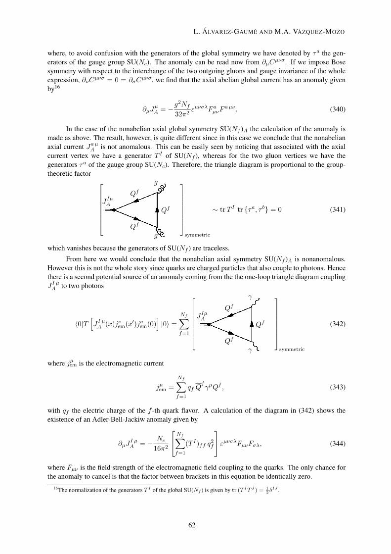
where, to avoid confusion with the generators of the global symmetry we have denoted by τa the gen-erators of the gauge group SU(Nc). The anomaly can be read now from ∂µC

µνσ. If we impose Bosesymmetry with respect to the interchange of the two outgoing gluons and gauge invariance of the wholeexpression, ∂νC

µνσ = 0 = ∂σCµνσ, we find that the axial abelian global current has an anomaly given

by16

∂µJµA = −g

2Nf

32π2εµνσλF a

µνFa µν . (340)

In the case of the nonabelian axial global symmetry SU(Nf )A the calculation of the anomaly ismade as above. The result, however, is quite different since in this case we conclude that the nonabelianaxial current Ja µ

A is not anomalous. This can be easily seen by noticing that associated with the axialcurrent vertex we have a generator T I of SU(Nf ), whereas for the two gluon vertices we have thegenerators τa of the gauge group SU(Nc). Therefore, the triangle diagram is proportional to the group-theoretic factor

JIµ

A

Qf

g

Qf

g

Qf

symmetric

∼ trT I tr τa, τ b = 0 (341)

which vanishes because the generators of SU(Nf ) are traceless.

From here we would conclude that the nonabelian axial symmetry SU(Nf )A is nonanomalous.However this is not the whole story since quarks are charged particles that also couple to photons. Hencethere is a second potential source of an anomaly coming from the the one-loop triangle diagram couplingJI µ

A to two photons

⟨0|T[JI µ

A (x)jνem(x′)jσ

em(0)]|0⟩ =

Nf∑

f=1

JIµ

A

Qf

γ

Qf

γ

Qf

symmetric

(342)

where jµem is the electromagnetic current

jµem =

Nf∑

f=1

qf QfγµQf , (343)

with qf the electric charge of the f -th quark flavor. A calculation of the diagram in (342) shows theexistence of an Adler-Bell-Jackiw anomaly given by

∂µJI µA = − Nc

16π2

Nf∑

f=1

(T I)ff q2f

εµνσλFµνFσλ, (344)

where Fµν is the field strength of the electromagnetic field coupling to the quarks. The only chance forthe anomaly to cancel is that the factor between brackets in this equation be identically zero.

16The normalization of the generators T I of the global SU(Nf ) is given by tr (T IT J) = 12δIJ .

62


62

Before proceeding let us summarize the results found so far. Because of the presence of anomaliesthe axial part of the global chiral symmetry, SU(Nf )A and U(1)A are not realized quantum mechanicallyin general. We found that U(1)A is always affected by an anomaly. However, because the right-handside of the anomaly equation (340) is a total derivative, the anomalous character of Jµ

A does not explainthe absence of U(1)A multiplets in the hadron spectrum, since a new current can be constructed whichis conserved. In addition, the nonexistence of candidates for a Goldstone boson associated with theright quantum numbers indicates that U(1)A is not spontaneously broken either, so it has be explicitlybroken somehow. This is the so-called U(1)-problem which was solved by ’t Hooft [33], who showedhow the contribution of quantum transitions between vacua with topologically nontrivial gauge fieldconfigurations (instantons) results in an explicit breaking of this symmetry.

Due to the dynamics of the SU(Nc) gauge theory the axial nonabelian symmetry is spontaneouslybroken due to the presence at low energies of a vacuum expectation value for the fermion bilinear Qf

Qf

⟨0|QfQf |0⟩ = 0 (No summation in f !). (345)

This nonvanishing vacuum expectation value for the quark bilinear actually breaks chiral invariancespontaneously to the vector subgroup SU(Nf )V , so the only subgroup of the original global symmetrythat is realized by the full theory at low energy is

U(Nf )L × U(Nf )R −→ SU(Nf )V × U(1)B. (346)

Associated with this breaking a Goldstone boson should appear with the quantum numbers of the brokennonabelian current. For example, in the case of QCD the Goldstone bosons associated with the sponta-neously symmetry breaking induced by the vacuum expectation values ⟨uu⟩, ⟨dd⟩ and ⟨(ud− du)⟩ havebeen identified as the pions π0, π±. These bosons are not exactly massless because of the nonvanishingmass of the u and d quarks. Since the global chiral symmetry is already slightly broken by mass terms inthe Lagrangian, the associated Goldstone bosons also have masses although they are very light comparedto the masses of other hadrons.

In order to have a better physical understanding of the role of anomalies in the physics of stronginteractions we particularize now our analysis of the case of real QCD. Since the u and d quarks aremuch lighter than the other four flavors, QCD at low energies can be well described by including onlythese two flavors and ignoring heavier quarks. In this approximation, from our previous discussion weknow that the low energy global symmetry of the theory is SU(2)V ×U(1)B , where now the vector groupSU(2)V is the well-known isospin symmetry. The axial U(1)A current is anomalous due to Eq. (340)with Nf = 2. In the case of the nonabelian axial symmetry SU(2)A, taking into account that qu = 2

3eand qd = −1

3e and that the three generators of SU(2) can be written in terms of the Pauli matrices asTK = 1

2σK we find

∑

f=u,d

(T 1)ff q2f =

∑

f=u,d

(T 1)ff q2f = 0,

∑

f=u,d

(T 3)ff q2f =

e2

6. (347)

Therefore J3 µA is anomalous.

Physically, the anomaly in the axial current J3 µA has an important consequence. In the quark

model, the wave function of the neutral pion π0 is given in terms of those for the u and d quark by

|π0⟩ =1√2

(|u⟩|u⟩ − |d⟩|d⟩

). (348)

The isospin quantum numbers of |π0⟩ are those of the generator T 3. Actually the analogy goes furthersince ∂µJ

3 µA is the operator creating a pion π0 out of the vacuum

|π0⟩ ∼ ∂µJ3 µA |0⟩. (349)

63


63

This leads to the physical interpretation of the triangle diagram (342) with J3 µA as the one loop contribu-

tion to the decay of a neutral pion into two photons

π0 −→ 2γ . (350)

This is an interesting piece of physics. In 1967 Sutherland and Veltman [34] presented a calcula-tion, using current algebra techniques, according to which the decay of the pion into two photons shouldbe suppressed. This however contradicted the experimental evidence that showed the existence of sucha decay. The way out to this paradox, as pointed out in [30], is the axial anomaly. What happens is thatthe current algebra analysis overlooks the ambiguities associated with the regularization of divergencesin Quantum Field Theory. A QED evaluation of the triangle diagram leads to a divergent integral thathas to be regularized somehow. It is in this process that the Adler-Bell-Jackiw axial anomaly appearsresulting in a nonvanishing value for the π0 → 2γ amplitude17.

The existence of anomalies associated with global currents does not necessarily mean difficultiesfor the theory. On the contrary, as we saw in the case of the axial anomaly it is its existence whatallows for a solution of the Sutherland-Veltman paradox and an explanation of the electromagnetic decayof the pion. The situation, however, is very different if we deal with local symmetries. A quantummechanical violation of gauge symmetry leads to all kinds of problems, from lack of renormalizability tonondecoupling of negative norm states. This is because the presence of an anomaly in the theory impliesthat the Gauss’ law constraint ∇ · Ea = ρa cannot be consistently implemented in the quantum theory.As a consequence states that classically are eliminated by the gauge symmetry become propagating fieldsin the quantum theory, thus spoiling the consistency of the theory.

Anomalies in a gauge symmetry can be expected only in chiral theories where left and right-handed fermions transform in different representations of the gauge group. Physically, the most interest-ing example of such theories is the electroweak sector of the Standard Model where, for example, lefthanded fermions transform as doublets under SU(2) whereas right-handed fermions are singlets. On theother hand, QCD is free of gauge anomalies since both left- and right-handed quarks transform in thefundamental representation of SU(3).

We consider the Lagrangian

L = −1

4F a µνF a

µν + i

N+∑

i=1

ψi+D/

(+)ψi+ + i

N−∑

j=1

ψj−D/

(−)ψj−, (351)

where the chiral fermions ψi± transform according to the representations τa

i,± of the gauge group G

(a = 1, . . . , dimG). The covariant derivatives D(±)µ are then defined by

D(±)µ ψi

± = ∂µψi± + igAK

µ τKi,±ψ

i±. (352)

As for global symmetries, anomalies in the gauge symmetry appear in the triangle diagram with oneaxial and two vector gauge current vertices

⟨0|T[ja µA (x)jb ν

V (x′)jc σV (0)

]|0⟩ =

jaµ

A

jbνV

jcσV

symmetric

(353)

17An early computation of the triangle diagram for the electromagnetic decay of the pion was made by Steinberger in [31].

64


64

where gauge vector and axial currents ja µV , ja µ

A are given by

jaµV =

N+∑

i=1

ψi+τ

a+γ

µψi+ +

N−∑

j=1

ψj−τ

a−γ

µψj−,

jaµA =

N+∑

i=1

ψi+τ

a+γ

µψi+ −

N−∑

i=1

ψj−τ

a−γ

µψj−. (354)

Luckily, we do not have to compute the whole diagram in order to find an anomaly cancellation condition,it is enough if we calculate the overall group theoretical factor. In the case of the diagram in Eq. (353)for every fermion species running in the loop this factor is equal to

tr[τai,±τ b

i,±, τci,±

], (355)

where the sign ± corresponds respectively to the generators of the representation of the gauge group forthe left and right-handed fermions. Hence the anomaly cancellation condition reads

N+∑

i=1

tr[τai,+τ b

i,+, τci,+

]−

N−∑

j=1

tr[τaj,−τ b

j,−, τcj,−

]= 0. (356)

Knowing this we can proceed to check the anomaly cancellation in the Standard ModelSU(3)×SU(2)×U(1). Left handed fermions (both leptons and quarks) transform as doublets with respectto the SU(2) factor whereas the right-handed components are singlets. The charge with respect to theU(1) part, the hypercharge Y , is determined by the Gell-Mann-Nishijima formula

Q = T3 + Y, (357)

where Q is the electric charge of the corresponding particle and T3 is the eigenvalue with respect to thethird generator of the SU(2) group in the corresponding representation: T3 = 1

2σ3 for the doublets and

T3 = 0 for the singlets. For the first family of quarks (u, d) and leptons (e, νe) we have the followingfield content

quarks:(uα

dα

)

L, 16

uαR, 2

3

dαR, 2

3

leptons:(νe

e

)

L,− 12

eR,−1 (358)

where α = 1, 2, 3 labels the color quantum number and the subscript indicates the value of the weakhypercharge Y . Denoting the representations of SU(3)×SU(2)×U(1) by (nc, nw)Y , with nc and nw

the representations of SU(3) and SU(2) respectively and Y the hypercharge, the matter content of theStandard Model consists of a three family replication of the representations:

left-handed fermions: (3, 2)L16

(1, 2)L− 1

2

(359)

right-handed fermions: (3, 1)R23

(3, 1)R− 1

3

(1, 1)R−1.

In computing the triangle diagram we have 10 possibilities depending on which factor of the gauge group

65


65

SU(3)×SU(2)×U(1) couples to each vertex:

SU(3)3 SU(2)3 U(1)3

SU(3)2 SU(2) SU(2)2 U(1)

SU(3)2 U(1) SU(2) U(1)2

SU(3) SU(2)2

SU(3) SU(2) U(1)

SU(3) U(1)2

It is easy to check that some of them do not give rise to anomalies. For example the anomaly for theSU(3)3 case cancels because left and right-handed quarks transform in the same representation. In thecase of SU(2)3 the cancellation happens term by term because of the Pauli matrices identity σaσb =δab + iεabcσc that leads to

tr[σaσb, σc

]= 2 (trσa) δbc = 0. (360)

However the hardest anomaly cancellation condition to satisfy is the one with three U(1)’s. In this casethe absence of anomalies within a single family is guaranteed by the nontrivial identity

∑

left

Y 3+ −

∑

right

Y 3− = 3 × 2 ×

(1

6

)3

+ 2 ×(

−1

2

)3

− 3 ×(

2

3

)3

− 3 ×(

−1

3

)3

− (−1)3

=

(−3

4

)+

(3

4

)= 0. (361)

It is remarkable that the anomaly exactly cancels between leptons and quarks. Notice that this resultholds even if a right-handed sterile neutrino is added since such a particle is a singlet under the wholeStandard Model gauge group and therefore does not contribute to the triangle diagram. Therefore we seehow the matter content of the Standard Model conspires to yield a consistent quantum field theory.

In all our discussion of anomalies we only considered the computation of one-loop diagrams.It may happen that higher loop orders impose additional conditions. Fortunately this is not so: theAdler-Bardeen theorem [35] guarantees that the axial anomaly only receives contributions from one loopdiagrams. Therefore, once anomalies are canceled (if possible) at one loop we know that there will beno new conditions coming from higher-loop diagrams in perturbation theory.

The Adler-Bardeen theorem, however, only applies in perturbation theory. It is nonetheless possi-ble that nonperturbative effects can result in the quantum violation of a gauge symmetry. This is preciselythe case pointed out by Witten [36] with respect to the SU(2) gauge symmetry of the Standard Model.In this case the problem lies in the nontrivial topology of the gauge group SU(2). The invariance ofthe theory with respect to gauge transformations which are not in the connected component of the iden-tity makes all correlation functions equal to zero. Only when the number of left-handed SU(2) fermiondoublets is even gauge invariance allows for a nontrivial theory. It is again remarkable that the familystructure of the Standard Model makes this anomaly to cancel

3 ×(ud

)

L

+ 1 ×(νe

e

)

L

= 4 SU(2)-doublets, (362)

where the factor of 3 comes from the number of colors.

66


66

8 Renormalization8.1 Removing infinitiesFrom its very early stages, Quantum Field Theory was faced with infinities. They emerged in the calcula-tion of most physical quantities, such as the correction to the charge of the electron due to the interactionswith the radiation field. The way these divergences where handled in the 1940s, starting with Kramers,was physically very much in the spirit of the Quantum Theory emphasis in observable quantities: sincethe observed magnitude of physical quantities (such as the charge of the electron) is finite, this numbershould arise from the addition of a “bare” (unobservable) value and the quantum corrections. The factthat both of these quantities were divergent was not a problem physically, since only its finite sum wasan observable quantity. To make thing mathematically sound, the handling of infinities requires the in-troduction of some regularization procedure which cuts the divergent integrals off at some momentumscale Λ. Morally speaking, the physical value of an observable Ophysical is given by

Ophysical = limΛ→∞

[O(Λ)bare + ∆O(Λ)ℏ] , (363)

where ∆O(Λ)ℏ represents the regularized quantum corrections.

To make this qualitative discussion more precise we compute the corrections to the electric chargein Quantum Electrodynamics. We consider the process of annihilation of an electron-positron pair tocreate a muon-antimuon pair e−e+ → µ+µ−. To lowest order in the electric charge e the only diagramcontributing is

!e− µ+

e+

γ

µ−

However, the corrections at order e4 to this result requires the calculation of seven more diagrams

"e− µ+

e+ µ−

+#e− µ+

e+

µ−

+$µ+e−

µ−e+

+%e− µ+

e+ µ−

+&e− µ+

e+

µ−+'µ+e+

µ−e−

+(µ+e+

µ−e−

In order to compute the renormalization of the charge we consider the first diagram which takesinto account the first correction to the propagator of the virtual photon interchanged between the pairs

67


67

due to vacuum polarization. We begin by evaluating

)=

−iηµα

q2 + iϵ

*α β

−iηβν

q2 + iϵ, (364)

where the diagram between brackets is given by

+α β ≡ Παβ(q) = i2(−ie)2(−1)

∫d4k

(2π)4Tr (/k +me)γ

α(/k + /q +me)γβ

[k2 −m2e + iϵ] [(k + q)2 −m2

e + iϵ]. (365)

Physically this diagram includes the correction to the propagator due to the polarization of the vacuum,i.e. the creation of virtual electron-positron pairs by the propagating photon. The momentum q is thetotal momentum of the electron-positron pair in the intermediate channel.

It is instructive to look at this diagram from the point of view of perturbation theory in nonrela-tivistic Quantum Mechanics. In each vertex the interaction consists of the annihilation (resp. creation)of a photon and the creation (resp. annihilation) of an electron-positron pair. This can be implementedby the interaction Hamiltonian

Hint = e

∫d3xψγµψAµ. (366)

All fields inside the integral can be expressed in terms of the corresponding creation-annihilation oper-ators for photons, electrons and positrons. In Quantum Mechanics, the change in the wave function atfirst order in the perturbation Hint is given by

|γ, in⟩ = |γ, in⟩0 +∑

n

⟨n|Hint|γ, in⟩0Ein −En

|n⟩ (367)

and similarly for |γ, out⟩, where we have denoted symbolically by |n⟩ all the possible states of theelectron-positron pair. Since these states are orthogonal to |γ, in⟩0, |γ, out⟩0, we find torder e2

⟨γ, in|γ′, out⟩ = 0⟨γ, in|γ′, out⟩0 +∑

n

0⟨γ, in|Hint|n⟩ ⟨n|Hint|γ′, out⟩0(Ein − En)(Eout − En)

+ O(e4). (368)

Hence, we see that the diagram of Eq. (364) really corresponds to the order-e2 correction to the photonpropagator ⟨γ, in|γ′, out⟩

,γ γ′−→ 0⟨γ, in|γ′, out⟩0

-γ γ′−→

∑

n

⟨γ, in|Hint|n⟩ ⟨n|Hint|γ′, out⟩(Ein −En)(Eout − En)

. (369)

68


68

Once we understood the physical meaning of the Feynman diagram to be computed we proceedto its evaluation. In principle there is no problem in computing the integral in Eq. (364) for nonzerovalues of the electron mass. However since here we are going to be mostly interested in seeing howthe divergence of the integral results in a scale-dependent renormalization of the electric charge, wewill set me = 0. This is something safe to do, since in the case of this diagram we are not inducingnew infrared divergences in taking the electron as massless. Implementing gauge invariance and usingstandard techniques in the computation of Feynman diagrams (see references [1]- [11]) the polarizationtensor Πµν(q) defined in Eq. (365) can be written as

Πµν(q) =(q2ηµν − qµqν

)Π(q2) (370)

with

Π(q) = 8e2∫ 1

0dx

∫d4k

(2π)4x(1 − x)

[k2 −m2 + x(1 − x)q2 + iϵ]2(371)

To handle this divergent integral we have to figure out some procedure to render it finite. This can bedone in several ways, but here we choose to cut the integrals off at a high energy scale Λ, where newphysics might be at work, |p| < Λ. This gives the result

Π(q2) ≃ e2

12π2log

(q2

Λ2

)+ finite terms. (372)

If we would send the cutoff to infinity Λ → ∞ the divergence blows up and something has to be doneabout it.

If we want to make sense out of this, we have to go back to the physical question that led us tocompute Eq. (364). Our primordial motivation was to compute the corrections to the annihilation of twoelectrons into two muons. Including the correction to the propagator of the virtual photon we have

. =/ +0= ηαβ (veγ

αue)e2

4πq2

(vµγ

βuµ

)+ ηαβ (veγ

αue)e2

4πq2Π(q2)

(vµγ

βuµ

)

= ηαβ (veγαue)

e2

4πq2

[1 +

e2

12π2log

(q2

Λ2

)](vµγ

βuµ

). (373)

Now let us imagine that we are performing a e− e+ → µ−µ+ with a center of mass energy µ. From theprevious result we can identify the effective charge of the particles at this energy scale e(µ) as

1 = ηαβ (veγαue)

[e(µ)2

4πq2

](vµγ

βuµ

). (374)

This charge, e(µ), is the quantity that is physically measurable in our experiment. Now we can makesense of the formally divergent result (373) by assuming that the charge appearing in the classical La-grangian of QED is just a “bare” value that depends on the scale Λ at which we cut off the theory,e ≡ e(Λ)bare. In order to reconcile (373) with the physical results (374) we must assume that thedependence of the bare (unobservable) charge e(Λ)bare on the cutoff Λ is determined by the identity

e(µ)2 = e(Λ)2bare

[1 +

e(Λ)2bare

12π2log

(µ2

Λ2

)]. (375)

69


69

If we still insist in removing the cutoff, Λ → ∞ we have to send the bare charge to zero e(Λ)bare → 0in such a way that the effective coupling has the finite value given by the experiment at the energy scaleµ. It is not a problem, however, that the bare charge is small for large values of the cutoff, since theonly measurable quantity is the effective charge that remains finite. Therefore all observable quantitiesshould be expressed in perturbation theory as a power series in the physical coupling e(µ)2 and not inthe unphysical bare coupling e(Λ)bare.

8.2 The beta-function and asymptotic freedomWe can look at the previous discussion, an in particular Eq. (375), from a different point of view. In orderto remove the ambiguities associated with infinities we have been forced to introduce a dependence ofthe coupling constant on the energy scale at which a process takes place. From the expression of thephysical coupling in terms of the bare charge (375) we can actually eliminate the cutoff Λ, whose valueafter all should not affect the value of physical quantities. Taking into account that we are working inperturbation theory in e(µ)2, we can express the bare charge e(Λ)2bare in terms of e(µ)2 as

e(Λ)2bare = e(µ)2[1 − e(µ)2

12π2log

(µ2

Λ2

)]+ O[e(µ)6]. (376)

This expression allow us to eliminate all dependence in the cutoff in the expression of the effective chargeat a scale µ by replacing e(Λ)bare in Eq. (375) by the one computed using (376) at a given referenceenergy scale µ0

e(µ)2 = e(µ0)2

[1 +

e(µ0)2

12π2log

(µ2

µ20

)]. (377)

From this equation we can compute, at this order in perturbation theory, the effective value of thecoupling constant at an energy µ, once we know its value at some reference energy scale µ0. In the caseof the electron charge we can use as a reference Thompson’s scattering at energies of the order of theelectron massme ≃ 0.5 MeV, at where the value of the electron charge is given by the well known value

e(me)2 ≃ 1

137. (378)

With this we can compute e(µ)2 at any other energy scale applying Eq. (377), for example at the electronmass µ = me ≃ 0.5 MeV. However, in computing the electromagnetic coupling constant at any otherscale we must take into account the fact that other charged particles can run in the loop in Eq. (373).Suppose, for example, that we want to calculate the fine structure constant at the mass of the Z0-bosonµ = MZ ≡ 92 GeV. Then we should include in Eq. (377) the effect of other fermionic Standard Modelfields with masses below MZ . Doing this, we find18

e(MZ)2 = e(me)2

[1 +

e(me)2

12π2

(∑

i

q2i

)log

(M2

Z

m2e

)], (379)

where qi is the charge in units of the electron charge of the i-th fermionic species running in the loopand we sum over all fermions with masses below the mass of the Z0 boson. This expression shows howthe electromagnetic coupling grows with energy. However, in order to compare with the experimentalvalue of e(MZ)2 it is not enough with including the effect of fermionic fields, since also the W± bosons

18In the first version of these notes the argument used to show the growing of the electromagnetic coupling constant couldhave led to confusion to some readers. To avoid this potential problem we include in the equation for the running couplinge(µ)2 the contribution of all fermions with masses below MZ . We thank Lubos Motl for bringing this issue to our attention.

70


70

can run in the loop (MW < MZ). Taking this into account, as well as threshold effects, the value of theelectron charge at the scale MZ is found to be [37]

e(MZ)2 ≃ 1

128.9. (380)

This growing of the effective fine structure constant with energy can be understood heuristicallyby remembering that the effect of the polarization of the vacuum shown in the diagram of Eq. (364)amounts to the creation of a plethora of electron-positron pairs around the location of the charge. Thesevirtual pairs behave as dipoles that, as in a dielectric medium, tend to screen this charge and decreasingits value at long distances (i.e. lower energies).

The variation of the coupling constant with energy is usually encoded in Quantum Field Theoryin the beta function defined by

β(g) = µdg

dµ. (381)

In the case of QED the beta function can be computed from Eq. (377) with the result

β(e)QED =e3

12π2. (382)

The fact that the coefficient of the leading term in the beta-function is positive β0 ≡ 16π > 0 gives

us the overall behavior of the coupling as we change the scale. Eq. (382) means that, if we start at anenergy where the electric coupling is small enough for our perturbative treatment to be valid, the effectivecharge grows with the energy scale. This growing of the effective coupling constant with energy meansthat QED is infrared safe, since the perturbative approximation gives better and better results as we go tolower energies. Actually, because the electron is the lighter electrically charged particle and has a finitenonvanishing mass the running of the fine structure constant stops at the scale me in the well-knownvalue 1

137 . Would other charged fermions with masses below me be present in Nature, the effective valueof the fine structure constant in the interaction between these particles would run further to lower valuesat energies below the electron mass.

On the other hand if we increase the energy scale e(µ)2 grows until at some scale the coupling is oforder one and the perturbative approximation breaks down. In QED this is known as the problem of theLandau pole but in fact it does not pose any serious threat to the reliability of QED perturbation theory:a simple calculation shows that the energy scale at which the theory would become strongly coupled isΛLandau ≃ 10277 GeV. However, we know that QED does not live that long! At much lower scales weexpect electromagnetism to be unified with other interactions, and even if this is not the case we willenter the uncharted territory of quantum gravity at energies of the order of 1019 GeV.

So much for QED. The next question that one may ask at this stage is whether it is possible tofind quantum field theories with a behavior opposite to that of QED, i.e. such that they become weaklycoupled at high energies. This is not a purely academic question. In the late 1960s a series of deep-inelastic scattering experiments carried out at SLAC showed that the quarks behave essentially as freeparticles inside hadrons. The apparent problem was that no theory was known at that time that wouldbecome free at very short distances: the example set by QED seem to be followed by all the theoriesthat were studied. This posed a very serious problem for Quantum Field Theory as a way to describesubnuclear physics, since it seemed that its predictive power was restricted to electrodynamics but failedmiserably when applied to describe strong interactions.

Nevertheless, this critical time for Quantum Field Theory turned out to be its finest hour. In 1973David Gross and Frank Wilczek [38] and David Politzer [39] showed that nonabelian gauge theories canactually display the required behavior. For the QCD Lagrangian in Eq. (331) the beta function is given

71


71

g

g

β( )g

g*1

g*2

*3

Fig. 14: Beta function for a hypothetical theory with three fixed points g∗1 , g∗

2 and g∗3 . A perturbative analysis

would capture only the regions shown in the boxes.

by19

β(g) = − g3

16π2

[11

3Nc − 2

3Nf

]. (383)

In particular, for real QCD (NC = 3, Nf = 6) we have that β(g) = − 7g3

16π2 < 0. This means thatfor a theory that is weakly coupled at an energy scale µ0 the coupling constant decreases as the energyincreases µ → ∞. This explain the apparent freedom of quarks inside the hadrons: when the quarksare very close together their effective color charge tend to zero. This phenomenon is called asymptoticfreedom.

Asymptotic free theories display a behavior that is opposite to that found above in QED. At highenergies their coupling constant approaches zero whereas at low energies they become strongly coupled(infrared slavery). This features are at the heart of the success of QCD as a theory of strong interactions,since this is exactly the type of behavior found in quarks: they are quasi-free particles inside the hadronsbut the interaction potential potential between them increases at large distances.

Although asymptotic free theories can be handled in the ultraviolet, they become extremely com-plicated in the infrared. In the case of QCD it is still to be understood (at least analytically) how thetheory confines color charges and generates the spectrum of hadrons, as well as the breaking of the chiralsymmetry (345).

In general, the ultraviolet and infrared properties of a theory are controlled by the fixed points ofthe beta function, i.e. those values of the coupling constant g for which it vanishes

β(g∗) = 0. (384)

Using perturbation theory we have seen that for both QED and QCD one of such fixed points occursat zero coupling, g∗ = 0. However, our analysis also showed that the two theories present radicallydifferent behavior at high and low energies. From the point of view of the beta function, the differencelies in the energy regime at which the coupling constant approaches its critical value. This is in factgoverned by the sign of the beta function around the critical coupling.

19The expression of the beta function of QCD was also known to ’t Hooft [40]. There are even earlier computations in therussian literature [41].

72


72

We have seen above that when the beta function is negative close to the fixed point (the case ofQCD) the coupling tends to its critical value, g∗ = 0, as the energy is increased. This means that thecritical point is ultraviolet stable, i.e. it is an attractor as we evolve towards higher energies. If, on thecontrary, the beta function is positive (as it happens in QED) the coupling constant approaches the criticalvalue as the energy decreases. This is the case of an infrared stable fixed point.

This analysis that we have motivated with the examples of QED and QCD is completely generaland can be carried out for any quantum field theory. In Fig. 14 we have represented the beta function fora hypothetical theory with three fixed points located at couplings g∗

1 , g∗2 and g∗

3 . The arrows in the linebelow the plot represent the evolution of the coupling constant as the energy increases. From the analysispresented above we see that g∗

1 = 0 and g∗3 are ultraviolet stable fixed points, while the fixed point g∗

2 isinfrared stable.

In order to understand the high and low energy behavior of a quantum field theory it is then crucialto know the structure of the beta functions associated with its couplings. This can be a very difficulttask, since perturbation theory only allows the study of the theory around “trivial" fixed points, i.e. thosethat occur at zero coupling like the case of g∗

1 in Fig. 14. On the other hand, any “nontrivial” fixedpoint occurring in a theory (like g∗

2 and g∗3) cannot be captured in perturbation theory and requires a full

nonperturbative analysis.

The moral to be learned from our discussion above is that dealing with the ultraviolet divergencesin a quantum field theory has the consequence, among others, of introducing an energy dependence inthe measured value of the coupling constants of the theory (for example the electric charge in QED).This happens even in the case of renormalizable theories without mass terms. These theories are scaleinvariant at the classical level because the action does not contain any dimensionful parameter. In thiscase the running of the coupling constants can be seen as resulting from a quantum breaking of classicalscale invariance: different energy scales in the theory are distinguished by different values of the couplingconstants. Remembering what we learned in Section 7, we conclude that classical scale invariance is ananomalous symmetry. One heuristic way to see how the conformal anomaly comes about is to noticethat the regularization of an otherwise scale invariant field theory requires the introduction of an energyscale (e.g. a cutoff). This breaking of scale invariance cannot be restored after renormalization.

Nevertheless, scale invariance is not lost forever in the quantum theory. It is recovered at thefixed points of the beta function where, by definition, the coupling does not run. To understand howthis happens we go back to a scale invariant classical field theory whose field ϕ(x) transform undercoordinate rescalings as

xµ −→ λxµ, ϕ(x) −→ λ−∆ϕ(λ−1x), (385)

where ∆ is called the canonical scaling dimension of the field. An example of such a theory is a masslessϕ4 theory in four dimensions

L =1

2∂µϕ∂

µϕ− g

4!ϕ4, (386)

where the scalar field has canonical scaling dimension ∆ = 1. The Lagrangian density transforms as

L −→ λ−4L[ϕ] (387)

and the classical action remains invariant20.

If scale invariance is preserved under quantization, the Green’s functions transform as

⟨Ω|T [ϕ′(x1) . . . ϕ′(xn)]|Ω⟩ = λnΛ⟨Ω|T [ϕ(λ−1x1) . . . ϕ(λ−1xn)]|Ω⟩. (388)

20In a D-dimensional theory the canonical scaling dimensions of the fields coincide with its engineering dimension: ∆ =D−2

2for bosonic fields and ∆ = D−1

2for fermionic ones. For a Lagrangian with no dimensionful parameters classical scale

invariance follows then from dimensional analysis.

73


73

Fig. 15: Systems of spins in a two-dimensional square lattice.

This is precisely what happens in a free theory. In an interacting theory the running of the couplingconstant destroys classical scale invariance at the quantum level. Despite of this, at the fixed points ofthe beta function the Green’s functions transform again according to (388) where ∆ is replaced by

∆anom = ∆ + γ∗. (389)

The canonical scaling dimension of the fields are corrected by γ∗, which is called the anomalous dimen-sion. They carry the dynamical information about the high-energy behavior of the theory.

8.3 The renormalization groupIn spite of its successes, the renormalization procedure presented above can be seen as some kind of pre-scription or recipe to get rid of the divergences in an ordered way. This discomfort about renormalizationwas expressed in occasions by comparing it with “sweeping the infinities under the rug”. However thanksto Ken Wilson to a large extent [42] the process of renormalization is now understood in a very profoundway as a procedure to incorporate the effects of physics at high energies by modifying the value of theparameters that appear in the Lagrangian.

Statistical mechanics. Wilson’s ideas are both simple and profound and consist in thinking aboutQuantum Field Theory as the analog of a thermodynamical description of a statistical system. To bemore precise, let us consider an Ising spin system in a two-dimensional square lattice as the one depictedin Fig 15. In terms of the spin variables si = ±1

2 , where i labels the lattice site, the Hamiltonian of thesystem is given by

H = −J∑

⟨i,j⟩si sj , (390)

where ⟨i, j⟩ indicates that the sum extends over nearest neighbors and J is the coupling constant betweenneighboring spins (here we consider that there is no external magnetic field). The starting point to studythe statistical mechanics of this system is the partition function defined as

Z =∑

sie−βH , (391)

where the sum is over all possible configurations of the spins and β = 1T is the inverse temperature.

For J > 0 the Ising model presents spontaneous magnetization below a critical temperature Tc, in anydimension higher than one. Away from this temperature correlations between spins decay exponentiallyat large distances

⟨sisj⟩ ∼ e− |xij |

ξ , (392)

74


74

Fig. 16: Decimation of the spin lattice. Each block in the upper lattice is replaced by an effective spin computedaccording to the rule (394). Notice also that the size of the lattice spacing is doubled in the process.

with |xij | the distance between the spins located in the i-th and j-th sites of the lattice. This expressionserves as a definition of the correlation length ξ which sets the characteristic length scale at which spinscan influence each other by their interaction through their nearest neighbors.

Suppose now that we are interested in a macroscopic description of this spin system. We cancapture the relevant physics by integrating out somehow the physics at short scales. A way in which thiscan be done was proposed by Leo Kadanoff [43] and consists in dividing our spin system in spin-blockslike the ones showed in Fig 16. Now we can construct another spin system where each spin-block of theoriginal lattice is replaced by an effective spin calculated according to some rule from the spins containedin each block Ba

si : i ∈ Ba −→ s (1)a . (393)

For example we can define the effective spin associated with the block Ba by taking the majority rulewith an additional prescription in case of a draw

s (1)a =

1

2sgn

(∑

i∈Ba

si

), (394)

where we have used the sign function, sign(x) ≡ x|x| , with the additional definition sgn(0) = 1. This

procedure is called decimation and leads to a new spin system with a doubled lattice space.

The idea now is to rewrite the partition function (391) only in terms of the new effective spinss

(1)a . Then we start by splitting the sum over spin configurations into two nested sums, one over the spin

blocks and a second one over the spins within each block

Z =∑

se−βH[si] =

∑

s (1)

∑

s∈Baδ

[s (1)a − sign

(∑

i∈Ba

si

)]e−βH[si]. (395)

75


75

The interesting point now is that the sum over spins inside each block can be written as the exponentialof a new effective Hamiltonian depending only on the effective spins, H(1)[s

(1)a ]

∑

s∈Baδ

[s (1)a − sign

(∑

i∈Ba

si

)]e−βH[si] = e−βH(1)[s

(1)a ]. (396)

The new Hamiltonian is of course more complicated

H(1) = −J (1)∑

⟨i,j⟩s(1)i s

(1)j + . . . (397)

where the dots stand for other interaction terms between the effective block spins. This new terms appearbecause in the process of integrating out short distance physics we induce interactions between the neweffective degrees of freedom. For example the interaction between the spin block variables s(1)

i will ingeneral not be restricted to nearest neighbors in the new lattice. The important point is that we havemanaged to rewrite the partition function solely in terms of this new (renormalized) spin variables s (1)

interacting through a new Hamiltonian H(1)

Z =∑

s (1)e−βH(1)[s

(1)a ]. (398)

Let us now think about the space of all possible Hamiltonians for our statistical system includingall kinds of possible couplings between the individual spins compatible with the symmetries of the sys-tem. If denote by R the decimation operation, our previous analysis shows that R defines a map in thisspace of Hamiltonians

R : H → H(1). (399)

At the same time the operation R replaces a lattice with spacing a by another one with double spacing2a. As a consequence the correlation length in the new lattice measured in units of the lattice spacing isdivided by two, R : ξ → ξ

2 .

Now we can iterate the operation R an indefinite number of times. Eventually we might reach aHamiltonian H⋆ that is not further modified by the operation R

HR−→ H(1) R−→ H(2) R−→ . . .

R−→ H⋆. (400)

The fixed point Hamiltonian H⋆ is scale invariant because it does not change as R is performed. Noticethat because of this invariance the correlation length of the system at the fixed point do not change underR. This fact is compatible with the transformation ξ → ξ

2 only if ξ = 0 or ξ = ∞. Here we will focusin the case of nontrivial fixed points with infinite correlation length.

The space of Hamiltonians can be parametrized by specifying the values of the coupling constantsassociated with all possible interaction terms between individual spins of the lattice. If we denote byOa[si] these (possibly infinite) interaction terms, the most general Hamiltonian for the spin system understudy can be written as

H[si] =∞∑

a=1

λaOa[si], (401)

where λa ∈ R are the coupling constants for the corresponding operators. These constants can be thoughtof as coordinates in the space of all Hamiltonians. Therefore the operation R defines a transformation inthe set of coupling constants

R : λa −→ λ(1)a . (402)

76


76

For example, in our case we started with a Hamiltonian in which only one of the coupling constantsis different from zero (say λ1 = −J). As a result of the decimation λ1 ≡ −J → −J (1) while someof the originally vanishing coupling constants will take a nonzero value. Of course, for the fixed pointHamiltonian the coupling constants do not change under the scale transformation R.

Physically the transformation R integrates out short distance physics. The consequence for physicsat long distances is that we have to replace our Hamiltonian by a new one with different values for thecoupling constants. That is, our ignorance of the details of the physics going on at short distances resultin a renormalization of the coupling constants of the Hamiltonian that describes the long range physicalprocesses. It is important to stress that although R is sometimes called a renormalization group trans-formation in fact this is a misnomer. Transformations between Hamiltonians defined by R do not forma group: since these transformations proceed by integrating out degrees of freedom at short scales theycannot be inverted.

In statistical mechanics fixed points under renormalization group transformations with ξ = ∞are associated with phase transitions. From our previous discussion we can conclude that the spaceof Hamiltonians is divided in regions corresponding to the basins of attraction of the different fixedpoints. We can ask ourselves now about the stability of those fixed points. Suppose we have a statisticalsystem described by a fixed-point Hamiltonian H⋆ and we perturb it by changing the coupling constantassociated with an interaction term O. This is equivalent to replace H⋆ by the perturbed Hamiltonian

H = H⋆ + δλO, (403)

where δλ is the perturbation of the coupling constant corresponding to O (we can also consider pertur-bations in more than one coupling constant). At the same time thinking of the λa’s as coordinates in thespace of all Hamiltonians this corresponds to moving slightly away from the position of the fixed point.

The question to decide now is in which direction the renormalization group flow will take theperturbed system. Working at first order in δλ there are three possibilities:

– The renormalization group flow takes the system back to the fixed point. In this case the corre-sponding interaction O is called irrelevant.

– R takes the system away from the fixed point. If this is what happens the interaction is calledrelevant.

– It is possible that the perturbation actually does not take the system away from the fixed point atfirst order in δλ. In this case the interaction is said to be marginal and it is necessary to go to higherorders in δλ in order to decide whether the system moves to or away the fixed point, or whetherwe have a family of fixed points.

Therefore we can picture the action of the renormalization group transformation as a flow in thespace of coupling constants. In Fig. 17 we have depicted an example of such a flow in the case of asystem with two coupling constants λ1 and λ2. In this example we find two fixed points, one at theorigin O and another at F for a finite value of the couplings. The arrows indicate the direction in whichthe renormalization group flow acts. The free theory at λ1 = λ2 = 0 is a stable fix point since anyperturbation δλ1, δλ2 > 0 makes the theory flow back to the free theory at long distances. On theother hand, the fixed point F is stable with respect to certain type of perturbations (along the line withincoming arrows) whereas for any other perturbations the system flows either to the free theory at theorigin or to a theory with infinite values for the couplings.

Quantum field theory. Let us see now how these ideas of the renormalization group apply toField Theory. Let us begin with a quantum field theory defined by the Lagrangian

L[ϕa] = L0[ϕa] +∑

i

giOi[ϕa], (404)

77


77

λ

λ2

1

F

OFig. 17: Example of a renormalization group flow.

where L0[ϕa] is the kinetic part of the Lagrangian and gi are the coupling constants associated with theoperators Oi[ϕa]. In order to make sense of the quantum theory we introduce a cutoff in momenta Λ. Inprinciple we include all operators Oi compatible with the symmetries of the theory.

In section 8.2 we saw how in the cases of QED and QCD, the value of the coupling constantchanged with the scale from its value at the scale Λ. We can understand now this behavior along the linesof the analysis presented above for the Ising model. If we would like to compute the effective dynamicsof the theory at an energy scale µ < Λ we only have to integrate out all physical models with energiesbetween the cutoff Λ and the scale of interest µ. This is analogous to what we did in the Ising model byreplacing the original spins by the block spins. In the case of field theory the effective action S[ϕa, µ] atscale µ can be written in the language of functional integration as

eiS[ϕ′a,µ] =

∫

µ<p<Λ

∏

a

Dϕa eiS[ϕa,Λ]. (405)

Here S[ϕa,Λ] is the action at the cutoff scale

S[ϕa,Λ] =

∫d4x

L0[ϕa] +

∑

i

gi(Λ)Oi[ϕa]

(406)

and the functional integral in Eq. (405) is carried out only over the field modes with momenta in therange µ < p < Λ. The action resulting from integrating out the physics at the intermediate scalesbetween Λ and µ depends not on the original field variable ϕa but on some renormalized field ϕ′

a. Atthe same time the couplings gi(µ) differ from their values at the cutoff scale gi(Λ). This is analogous towhat we learned in the Ising model: by integrating out short distance physics we ended up with a newHamiltonian depending on renormalized effective spin variables and with renormalized values for thecoupling constants. Therefore the resulting effective action at scale µ can be written as

S[ϕ′a, µ] =

∫d4x

L0[ϕ

′a] +

∑

i

gi(µ)Oi[ϕ′a]

. (407)

This Wilsonian interpretation of renormalization sheds light to what in section 8.1 might have lookedjust a smart way to get rid of the infinities. The running of the coupling constant with the energy scalecan be understood now as a way of incorporating into an effective action at scale µ the effects of fieldexcitations at higher energies E > µ.

78


78

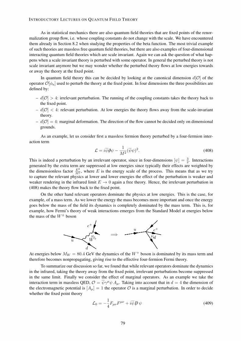
As in statistical mechanics there are also quantum field theories that are fixed points of the renor-malization group flow, i.e. whose coupling constants do not change with the scale. We have encounteredthem already in Section 8.2 when studying the properties of the beta function. The most trivial exampleof such theories are massless free quantum field theories, but there are also examples of four-dimensionalinteracting quantum field theories which are scale invariant. Again we can ask the question of what hap-pens when a scale invariant theory is perturbed with some operator. In general the perturbed theory is notscale invariant anymore but we may wonder whether the perturbed theory flows at low energies towardsor away the theory at the fixed point.

In quantum field theory this can be decided by looking at the canonical dimension d[O] of theoperator O[ϕa] used to perturb the theory at the fixed point. In four dimensions the three possibilities aredefined by:

– d[O] > 4: irrelevant perturbation. The running of the coupling constants takes the theory back tothe fixed point.

– d[O] < 4: relevant perturbation. At low energies the theory flows away from the scale-invarianttheory.

– d[O] = 4: marginal deformation. The direction of the flow cannot be decided only on dimensionalgrounds.

As an example, let us consider first a massless fermion theory perturbed by a four-fermion inter-action term

L = iψ∂/ψ − 1

M2(ψψ)2. (408)

This is indeed a perturbation by an irrelevant operator, since in four-dimensions [ψ] = 32 . Interactions

generated by the extra term are suppressed at low energies since typically their effects are weighted bythe dimensionless factor E2

M2 , where E is the energy scale of the process. This means that as we tryto capture the relevant physics at lower and lower energies the effect of the perturbation is weaker andweaker rendering in the infrared limit E → 0 again a free theory. Hence, the irrelevant perturbation in(408) makes the theory flow back to the fixed point.

On the other hand relevant operators dominate the physics at low energies. This is the case, forexample, of a mass term. As we lower the energy the mass becomes more important and once the energygoes below the mass of the field its dynamics is completely dominated by the mass term. This is, forexample, how Fermi’s theory of weak interactions emerges from the Standard Model at energies belowthe mass of the W± boson

2ue+

d

W+νe

=⇒3u e+

dνe

At energies below MW = 80.4 GeV the dynamics of the W+ boson is dominated by its mass term andtherefore becomes nonpropagating, giving rise to the effective four-fermion Fermi theory.

To summarize our discussion so far, we found that while relevant operators dominate the dynamicsin the infrared, taking the theory away from the fixed point, irrelevant perturbations become suppressedin the same limit. Finally we consider the effect of marginal operators. As an example we take theinteraction term in massless QED, O = ψγµψAµ. Taking into account that in d = 4 the dimension ofthe electromagnetic potential is [Aµ] = 1 the operator O is a marginal perturbation. In order to decidewhether the fixed point theory

L0 = −1

4FµνF

µν + iψD/ ψ (409)

79


79

is restored at low energies or not we need to study the perturbed theory in more detail. This we havedone in section 8.1 where we learned that the effective coupling in QED decreases at low energies. Thenwe conclude that the perturbed theory flows towards the fixed point in the infrared.

As an example of a marginal operator with the opposite behavior we can write the Lagrangian fora SU(Nc) gauge theory, L = −1

4FaµνF

a µν , as

L = −1

4

(∂µA

aν − ∂νA

aµ

)(∂µAa ν − ∂νAa µ) − 4gfabcAa

µAbν ∂

µAc ν

+ g2fabcfadeAbµA

cνA

d µAe ν ≡ L0 + Og, (410)

i.e. a marginal perturbation of the free theory described by L0, which is obviously a fixed point underrenormalization group transformations. Unlike the case of QED we know that the full theory is asymp-totically free, so the coupling constant grows at low energies. This implies that the operator Og becomesmore and more important in the infrared and therefore the theory flows away the fixed point in this limit.

It is very important to notice here that in the Wilsonian view the cutoff is not necessarily regardedas just some artifact to remove infinities but actually has a physical origin. For example in the case ofFermi’s theory of β-decay there is a natural cutoff Λ = MW at which the theory has to be replaced bythe Standard Model. In the case of the Standard Model itself the cutoff can be taken at Planck scaleΛ ≃ 1019 GeV or the Grand Unification scale Λ ≃ 1016 GeV, where new degrees of freedom areexpected to become relevant. The cutoff serves the purpose of cloaking the range of energies at whichnew physics has to be taken into account.

Provided that in the Wilsonian approach the quantum theory is always defined with a physicalcutoff, there is no fundamental difference between renormalizable and nonrenormalizable theories. Ac-tually, a renormalizable field theory, like the Standard Model, can generate nonrenormalizable operatorsat low energies such as the effective four-fermion interaction of Fermi’s theory. They are not sourcesof any trouble if we are interested in the physics at scales much below the cutoff, E ≪ Λ, since theircontribution to the amplitudes will be suppressed by powers of E

Λ .

9 Special topics9.1 Creation of particles by classical fieldsParticle creation by a classical source. In a free quantum field theory the total number of particlescontained in a given state of the field is a conserved quantity. For example, in the case of the quantumscalar field studied in section 3 we have that the number operator commutes with the Hamiltonian

n ≡∫

d3k

(2π)31

2ωkα†(k)α(k), [H, n] = 0. (411)

This means that any states with a well-defined number of particle excitations will preserve this numberat all times. The situation, however, changes as soon as interactions are introduced, since in this caseparticles can be created and/or destroyed as a result of the dynamics.

Another case in which the number of particles might change is if the quantum theory is coupledto a classical source. The archetypical example of such a situation is the Schwinger effect, in which aclassical strong electric field produces the creation of electron-positron pairs out of the vacuum. However,before plunging into this more involved situation we can illustrate the relevant physics involved in thecreation of particles by classical sources with the help of the simplest example: a free scalar field theorycoupled to a classical external source J(x). The action for such a theory can be written as

S =

∫d4x

[1

2∂µϕ(x)∂µϕ(x) − m2

2ϕ(x)2 + J(x)ϕ(x)

], (412)

80


80

where J(x) is a real function of the coordinates. Its identification with a classical source is obvious oncewe calculate the equations of motion

(∇2 +m2

)ϕ(x) = J(x). (413)

Our plan is to quantize this theory but, unlike the case analyzed in section 3, now the presence of thesource J(x) makes the situation a bit more involved. The general solution to the equations of motion canbe written in terms of the retarded Green function for the Klein-Gordon equation as

ϕ(x) = ϕ0(x) + i

∫d4x′GR(x− x′)J(x′), (414)

where ϕ0(x) is a general solution to the homogeneous equation and

GR(t, x) =

∫d4k

(2π)4i

k2 −m2 + iϵ sign(k0)e−ik·x

= i θ(t)

∫d3k

(2π)31

2ωk

(e−iωkt+k·x − eiωkt−ip·x

), (415)

with θ(x) the Heaviside step function. The integration contour to evaluate the integral over p0 surroundsthe poles at p0 = ±ωk from above. Since GR(t, x) = 0 for t < 0, the function ϕ0(x) corresponds to thesolution of the field equation at t → −∞, before the interaction with the external source21

To make the argument simpler we assume that J(x) is switched on at t = 0, and only last for atime τ , that is

J(t, x) = 0 if t < 0 or t > τ. (416)

We are interested in a solution of (413) for times after the external source has been switched off, t > τ .In this case the expression (415) can be written in terms of the Fourier modes J(ω, k) of the source as

ϕ(t, x) = ϕ0(x) + i

∫d3k

(2π)31

2ωk

[J(ωk, k)e

−iωkt+ik·x − J(ωk, k)∗eiωkt−ik·x

]. (417)

On the other hand, the general solution ϕ0(x) has been already computed in Eq. (77). Combining thisresult with Eq. (417) we find the following expression for the late time general solution to the Klein-Gordon equation in the presence of the source

ϕ(t, x) =

∫d3k

(2π)31√2ωk

[α(k) +

i√2ωk

J(ωk, k)

]e−iωkt+ik·x

+

[α∗(k) − i√

2ωkJ(ωk, k)

∗]eiωkt−ik·x

. (418)

We should not forget that this is a solution valid for times t > τ , i.e. once the external source has beendisconnected. On the other hand, for t < 0 we find from Eqs. (414) and (415) that the general solutionis given by Eq. (77).

Now we can proceed to quantize the theory. The conjugate momentum π(x) = ∂0ϕ(x) can becomputed from Eqs. (77) and (418). Imposing the canonical equal time commutation relations (74) wefind that α(k), α†(k) satisfy the creation-annihilation algebra (51). From our previous calculation wefind that for t > τ the expansion of the operator ϕ(x) in terms of the creation-annihilation operatorsα(k), α†(k) can be obtained from the one for t < 0 by the replacement

α(k) −→ β(k) ≡ α(k) +i√2ωk

J(ωk, k),

21We could have taken instead the advanced propagator GA(x) in which case ϕ0(x) would correspond to the solution to theequation at large times, after the interaction with J(x).

81


81

α†(k) −→ β†(k) ≡ α†(k) − i√2ωk

J(ωk, k)∗. (419)

Actually, since J(ωk, k) is a c-number, the operators β(k), β†(k) satisfy the same algebra as α(k), α†(k)and therefore can be interpreted as well as a set of creation-annihilation operators. This means that wecan define two vacuum states, |0−⟩, |0+⟩ associated with both sets of operators

α(k)|0−⟩ = 0

β(k)|0+⟩ = 0

∀ k. (420)

For an observer at t < 0, α(k) and α(k) are the natural set of creation-annihilation operatorsin terms of which to expand the field operator ϕ(x). After the usual zero-point energy subtraction theHamiltonian is given by

H(−) =1

2

∫d3k

(2π)3α†(k)α(k) (421)

and the ground state of the spectrum for this observer is the vacuum |0−⟩. At the same time, a secondobserver at t > τ will also see a free scalar quantum field (the source has been switched off at t = τ ) andconsequently will expand ϕ in terms of the second set of creation-annihilation operators β(k), β†(k). Interms of this operators the Hamiltonian is written as

H(+) =1

2

∫d3k

(2π)3β†(k)β(k). (422)

Then for this late-time observer the ground state of the Hamiltonian is the second vacuum state |0+⟩.In our analysis we have been working in the Heisenberg picture, where states are time-independent

and the time dependence comes in the operators. Therefore the states of the theory are globally defined.Suppose now that the system is in the “in” ground state |0−⟩. An observer at t < 0 will find that thereare no particles

n(−)|0−⟩ = 0. (423)

However the late-time observer will find that the state |0−⟩ contains an average number of particles givenby

⟨0−|n(+)|0−⟩ =

∫d3k

(2π)31

2ωk

∣∣∣J(ωk, k)∣∣∣2. (424)

Moreover, |0−⟩ is no longer the ground state for the “out” observer. On the contrary, this state have avacuum expectation value for H(+)

⟨0−|H(+)|0−⟩ =1

2

∫d3k

(2π)3

∣∣∣J(ωk, k)∣∣∣2. (425)

The key to understand what is going on here lies in the fact that the external source breaks theinvariance of the theory under space-time translations. In the particular case we have studied here whereJ(x) has support over a finite time interval 0 < t < τ , this implies that the vacuum is not invariantunder time translations, so observers at different times will make different choices of vacuum that willnot necessarily agree with each other. This is clear in our example. An observer in t < τ will choose thevacuum to be the lowest energy state of her Hamiltonian, |0−⟩. On the other hand, the second observerat late times t > τ will naturally choose |0+⟩ as the vacuum. However, for this second observer, the

82


82

E

x

e + 0

Dirac sea

e −

−m

m

E

0 L

Fig. 18: Pair creation by a electric field in the Dirac sea picture.

state |0−⟩ is not the vacuum of his Hamiltonian, but actually an excited state that is a superposition ofstates with well-defined number of particles. In this sense it can be said that the external source has theeffect of creating particles out of the “in” vacuum. Besides, this breaking of time translation invarianceproduces a violation in the energy conservation as we see from Eq. (425). Particles are actually createdfrom the energy pumped into the system by the external source.

The Schwinger effect. A classical example of creation of particles by a external field was pointedout by Schwinger [44] and consists of the creation of electron-positron pairs by a strong electric field. Inorder to illustrate this effect we are going to follow a heuristic argument based on the Dirac sea pictureand the WKB approximation.

In the absence of an electric field the vacuum state of a spin-12 field is constructed by filling all the

negative energy states as depicted in Fig. 2. Let us now connect a constant electric field E = E ux in therange 0 < x < L created by a electrostatic potential

V (r) =

0 x < 0−Ex 0 < x < L−EL x > L

(426)

After the field has been switched on, the Dirac sea looks like in Fig. 18. In particular we find that ifeEL > 2m there are negative energy states at x > L with the same energy as the positive energy statesin the region x < 0. Therefore it is possible for an electron filling a negative energy state with energyclose to −2m to tunnel through the forbidden region into a positive energy state. The interpretation ofsuch a process is the production of an electron-positron pair out of the electric field.

We can compute the rate at which such pairs are produced by using the WKB approximation.Focusing for simplicity on an electron on top of the Fermi surface near x = L with energy E0, thetransmission coefficient in this approximation is given by22

TWKB = exp

[−2

∫ 1eE

(E0+

√m2+p 2

T

)

1eE

(E0−

√m2+p 2

T

) dx

√m2 − [E0 − eE(x− x0)]

2 + p 2T

]

22Notice that the electron satisfy the relativistic dispersion relation E =√

p 2 + m2 + V and therefore −p2x = m2 − (E −

V )2 + p 2T . The integration limits are set by those values of x at which px = 0.

83


83

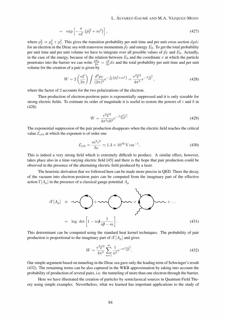
= exp[− π

eE(p 2

T +m2)], (427)

where p2T ≡ p2

y + p2z . This gives the transition probability per unit time and per unit cross section dydz

for an electron in the Dirac sea with transverse momentum pT and energyE0. To get the total probabilityper unit time and per unit volume we have to integrate over all possible values of pT and E0. Actually,in the case of the energy, because of the relation between E0 and the coordinate x at which the particlepenetrates into the barrier we can write dE0

2π = eE2πdx and the total probability per unit time and per unit

volume for the creation of a pair is given by

W = 2

(eE2π

)∫d2pT

(2π)2e−

πeE (p 2

T +m2) =e2E2

4π3e−

π m2

eE , (428)

where the factor of 2 accounts for the two polarizations of the electron.

Then production of electron-positron pairs is exponentially suppressed and it is only sizeable forstrong electric fields. To estimate its order of magnitude it is useful to restore the powers of c and ℏ in(428)

W =e2E2

4π3cℏ2e−

π m2c3

ℏeE (429)

The exponential suppression of the pair production disappears when the electric field reaches the criticalvalue Ecrit at which the exponent is of order one

Ecrit =m2c3

ℏe≃ 1.3 × 1016 V cm−1. (430)

This is indeed a very strong field which is extremely difficult to produce. A similar effect, however,takes place also in a time-varying electric field [45] and there is the hope that pair production could beobserved in the presence of the alternating electric field produced by a laser.

The heuristic derivation that we followed here can be made more precise in QED. There the decayof the vacuum into electron-positron pairs can be computed from the imaginary part of the effectiveaction Γ[Aµ] in the presence of a classical gauge potential Aµ

iΓ[Aµ] ≡4+5 +6 + . . .

= log det

[1 − ie/A

1

i∂/−m

]. (431)

This determinant can be computed using the standard heat kernel techniques. The probability of pairproduction is proportional to the imaginary part of iΓ[Aµ] and gives

W =e2E2

4π3

∞∑

n=1

1

n2e−n π m2

eE . (432)

Our simple argument based on tunneling in the Dirac sea gave only the leading term of Schwinger’s result(432). The remaining terms can be also captured in the WKB approximation by taking into account theprobability of production of several pairs, i.e. the tunneling of more than one electron through the barrier.

Here we have illustrated the creation of particles by semiclassical sources in Quantum Field The-ory using simple examples. Nevertheless, what we learned has important applications to the study of

84


84

quantum fields in curved backgrounds. In Quantum Field Theory in Minkowski space-time the vacuumstate is invariant under the Poincaré group and this, together with the covariance of the theory underLorentz transformations, implies that all inertial observers agree on the number of particles containedin a quantum state. The breaking of such invariance, as happened in the case of coupling to a time-varying source analyzed above, implies that it is not possible anymore to define a state which would berecognized as the vacuum by all observers.

This is precisely the situation when fields are quantized on curved backgrounds. In particular, ifthe background is time-dependent (as it happens in a cosmological setup or for a collapsing star) differentobservers will identify different vacuum states. As a consequence what one observer call the vacuum willbe full of particles for a different observer. This is precisely what is behind the phenomenon of Hawkingradiation [46]. The emission of particles by a physical black hole formed from gravitational collapse ofa star is the consequence of the fact that the vacuum state in the asymptotic past contain particles for anobserver in the asymptotic future. As a consequence, a detector located far away from the black holedetects a stream of thermal radiation with temperature

THawking =ℏc3

8πGN kM(433)

where M is the mass of the black hole, GN is Newton’s constant and k is Boltzmann’s constant. Thereare several ways in which this results can be obtained. A more heuristic way is perhaps to think of thisparticle creation as resulting from quantum tunneling of particles across the potential barrier posed bygravity [47].

9.2 SupersymmetryOne of the things that we have learned in our journey around the landscape of Quantum Field Theoryis that our knowledge of the fundamental interactions in Nature is based on the idea of symmetry, andin particular gauge symmetry. The Lagrangian of the Standard Model can be written just including allpossible renormalizable terms (i.e. with canonical dimension smaller o equal to 4) compatible with thegauge symmetry SU(3)×SU(2)×U(1) and Poincaré invariance. All attempts to go beyond start with thequestion of how to extend the symmetries of the Standard Model.

As explained in Section 5.1, in a quantum field theoretical description of the interaction of elemen-tary particles the basic observable quantity to compute is the scattering or S-matrix giving the probabilityamplitude for the scattering of a number of incoming particles with a certain momentum into some finalproducts

A(in −→ out) = ⟨p1′, . . . ; out|p1, . . . ; in⟩. (434)

An explicit symmetry of the theory has to be necessarily a symmetry of the S-matrix. Hence it is fair toask what is the largest symmetry of the S-matrix.

Let us ask this question in the simple case of the scattering of two particles with four-momenta p1

and p2 in the t-channel

7p1

p2

p′1

p′2

We will make the usual assumptions regarding positivity of the energy and analyticity. Invariance of thetheory under the Poincaré group implies that the amplitude can only depend on the scattering angle ϑthrough

t = (p′1 − p1)

2 = 2(m2

1 − p1 · p′1

)= 2

(m2

1 − E1E′1 + |p1||p1

′| cosϑ). (435)

85


85

If there would be any extra bosonic symmetry of the theory it would restrict the scattering angle to a setof discrete values. In this case the S-matrix cannot be analytic since it would vanish everywhere exceptfor the discrete values selected by the extra symmetry.

Actually, the only way to extend the symmetry of the theory without renouncing to the analyticityof the scattering amplitudes is to introduce “fermionic” symmetries, i.e. symmetries whose generatorsare anticommuting objects [48]. This means that in addition to the generators of the Poincaré group23

Pµ,Mµν and the ones for the internal gauge symmetriesG, we can introduce a number of fermionic gen-erators QI

a, Qa I (I = 1, . . . ,N ), where Qa I = (QIa)

†. The most general algebra that these generatorssatisfy is the N -extended supersymmetry algebra [49]

QIa, Qb J = 2σµ

abPµδ

IJ ,

QIa, Q

Jb = 2εabZIJ , (436)

QIa, Q

Jb = 2εabZ

IJ, (437)

where ZIJ ∈ C commute with any other generator and satisfies ZIJ = −ZJI . Besides we have thecommutators that determine the Poincaré transformations of the fermionic generators QI

a, Qa J

[QIa, P

µ] = [Qa I , Pµ] = 0,

[QIa,M

µν ] =1

2(σµν) b

a QIb , (438)

[Qa I ,Mµν ] = −1

2(σµν) b

a Qb I ,

where σ0i = −iσi, σij = εijkσk and σµν = (σµν)†. These identities simply mean that QIa, Qa J

transform respectively in the (12 ,0) and (0, 1

2) representations of the Lorentz group.

We know that the presence of a global symmetry in a theory implies that the spectrum can beclassified in multiplets with respect to that symmetry. In the case of supersymmetry start with the casecase N = 1 in which there is a single pair of supercharges Qa, Qa satisfying the algebra

Qa, Qb = 2σµ

abPµ, Qa, Qb = Qa, Qb = 0. (439)

Notice that in the N = 1 case there is no possibility of having central charges.

We study now the representations of the supersymmetry algebra (439), starting with the masslesscase. Given a state |k⟩ satisfying k2 = 0, we can always find a reference frame where the four-vector kµ

takes the form kµ = (E, 0, 0, E). Since the theory is Lorentz covariant we can obtain the representationof the supersymmetry algebra in this frame where the expressions are simpler. In particular, the right-hand side of the first anticommutator in Eq. (439) is given by

2σµ

abPµ = 2(P 0 − σ3P 3) =

(0 00 4E

). (440)

Therefore the algebra of supercharges in the massless case reduces to

Q1, Q†1 = Q1, Q

†2 = 0,

Q2, Q†2 = 4E. (441)

The commutator Q1, Q†1 = 0 implies that the action of Q1 on any state gives a zero-norm state of the

Hilbert space ||Q1|Ψ⟩|| = 0. If we want the theory to preserve unitarity we must eliminate these null

23The generators Mµν are related with the ones for boost and rotations introduced in section 4.1 by J i ≡ M0i, M i =12εijkM jk. In this section we also use the “dotted spinor” notation, in which spinors in the (1

2,0) and (0, 1

2) representations

of the Lorentz group are indicated respectively by undotted (a, b, . . .) and dotted (a, b, . . .) indices.

86


86

states from the spectrum. This is equivalent to setting Q1 ≡ 0. On the other hand, in terms of the secondgenerator Q2 we can define the operators

a =1

2√EQ2, a† =

1

2√EQ†

2, (442)

which satisfy the algebra of a pair of fermionic creation-annihilation operators, a, a† = 1, a2 =(a†)2 = 0. Starting with a vacuum state a|λ⟩ = 0 with helicity λ we can build the massless multiplet

|λ⟩, |λ+ 12⟩ ≡ a†|λ⟩. (443)

Here we consider two important cases:

– Scalar multiplet: we take the vacuum state to have zero helicity |0+⟩ so the multiplet consists of ascalar and a helicity-1

2 state

|0+⟩, | 12⟩ ≡ a†|0+⟩. (444)

However, this multiplet is not invariant under the CPT transformation which reverses the sign ofthe helicity of the states. In order to have a CPT-invariant theory we have to add to this multipletits CPT-conjugate which can be obtain from a vacuum state with helicity λ = −1

2

|0−⟩, | −12⟩. (445)

Putting them together we can combine the two zero helicity states with the two fermionic ones intothe degrees of freedom of a complex scalar field and a Weyl (or Majorana) spinor.

– Vector multiplet: now we take the vacuum state to have helicity λ = 12 , so the multiplet contains

also a massless state with helicity λ = 1

| 12⟩, |1⟩ ≡ a†| 1

2⟩. (446)

As with the scalar multiplet we add the CPT conjugated obtained from a vacuum state with helicityλ = −1

| − 12⟩, | − 1⟩, (447)

which together with (446) give the propagating states of a gauge field and a spin-12 gaugino.

In both cases we see the trademark of supersymmetric theories: the number of bosonic and fermionicstates within a multiplet are the same.

In the case of extended supersymmetry we have to repeat the previous analysis for each supersym-metry charge. At the end, we have N sets of fermionic creation-annihilation operators aI , a†

I = δIJ ,

(aI)2 = (a†

I)2 = 0. Let us work out the case of N = 8 supersymmetry. Since for several reasons we do

not want to have states with helicity larger than 2, we start with a vacuum state |−2⟩ of helicity λ = −2.The rest of the states of the supermultiplet are obtained by applying the eight different creation operatorsa†

I to the vacuum:

λ = 2 : a†1 . . . a

†8| − 2⟩

(8

8

)= 1 state,

λ =3

2: a†

I1. . . a†

I7| − 2⟩

(8

7

)= 8 states,

λ = 1 : a†I1. . . a†

I6| − 2⟩

(8

6

)= 28 states,

87


87

λ =1

2: a†

I1. . . a†

I5| − 2⟩

(8

5

)= 56 states,

λ = 0 : a†I1. . . a†

I4| − 2⟩

(8

4

)= 70 states, (448)

λ = −1

2: a†

I1a†

I2a†

I3| − 2⟩

(8

3

)= 56 states,

λ = −1 : a†I1a†

I2| − 2⟩

(8

2

)= 28 states,

λ = −3

2: a†

I1| − 2⟩

(8

1

)= 8 states,

λ = −2 : | − 2⟩ 1 state.

Putting together the states with opposite helicity we find that the theory contains:

– 1 spin-2 field gµν (a graviton),– 8 spin-3

2 gravitino fields ψIµ,

– 28 gauge fields A[IJ ]µ ,

– 56 spin-12 fermions ψ[IJK],

– 70 scalars ϕ[IJKL],

where by [IJ...] we have denoted that the indices are antisymmetrized. We see that, unlike the masslessmultiplets of N = 1 supersymmetry studied above, this multiplet is CPT invariant by itself. As in thecase of the massless N = 1 multiplet, here we also find as many bosonic as fermionic states:

bosons: 1 + 28 + 70 + 28 + 1 = 128 states,fermions: 8 + 56 + 56 + 8 = 128 states.

Now we study briefly the case of massive representations |k⟩, k2 = M2. Things become simplerif we work in the rest frame where P 0 = M and the spatial components of the momentum vanish. Then,the supersymmetry algebra becomes:

QIa, Qb J = 2Mδabδ

IJ . (449)

We proceed now in a similar way to the massless case by defining the operators

aIa ≡ 1√

2MQI

a, a†a I ≡ 1√

2MQa I . (450)

The multiplets are found by choosing a vacuum state with a definite spin. For example, for N = 1 andtaking a spin-0 vacuum |0⟩ we find three states in the multiplet transforming irreducibly with respect tothe Lorentz group:

|0⟩, a†a|0⟩, εaba†

aa†b|0⟩, (451)

which, once transformed back from the rest frame, correspond to the physical states of two spin-0 bosonsand one spin-1

2 fermion. For N -extended supersymmetry the corresponding multiplets can be workedout in a similar way.

The equality between bosonic and fermionic degrees of freedom is at the root of many of theinteresting properties of supersymmetric theories. For example, in section 4 we computed the divergentvacuum energy contributions for each real bosonic or fermionic propagating degree of freedom is24

Evac = ±1

2δ(0)

∫d3pωp, (452)

24For a boson, this can be read off Eq. (80). In the case of fermions, the result of Eq. (134) gives the vacuum energycontribution of the four real propagating degrees of freedom of a Dirac spinor.

88


88

where the sign ± corresponds respectively to bosons and fermions. Hence, for a supersymmetric the-ory the vacuum energy contribution exactly cancels between bosons and fermions. This boson-fermiondegeneracy is also responsible for supersymmetric quantum field theories being less divergent than non-supersymmetric ones.

Appendix: A crash course in Group TheoryIn this Appendix we summarize some basic facts about Group Theory. Given a group G a representationof G is a correspondence between the elements of G and the set of linear operators acting on a vectorspace V , such that for each element of the group g ∈ G there is a linear operator D(g)

D(g) : V −→ V (453)

satisfying the group operations

D(g1)D(g2) = D(g1g2), D(g−11 ) = D(g1)

−1, g1, g2 ∈ G. (454)

The representation D(g) is irreducible if and only if the only operators A : V → V commuting with allthe elements of the representation D(g) are the ones proportional to the identity

[D(g), A] = 0, ∀g ⇐⇒ A = λ1, λ ∈ C (455)

More intuitively, we can say that a representation is irreducible if there is no proper subspace U ⊂ V(i.e. U = V and U = ∅) such that D(g)U ⊂ U for every element g ∈ G.

Here we are specially interested in Lie groups whose elements are labelled by a number of con-tinuous parameters. In mathematical terms this means that a Lie group is a manifold M together withan operation M × M −→ M that we will call multiplication that satisfies the associativity propertyg1 · (g2 · g3) = (g1 · g2) · g3 together with the existence of unity g1 = 1g = g,for every g ∈ M andinverse gg−1 = g−1g = 1.

The simplest example of a Lie group is SO(2), the group of rotations in the plane. Each elementR(θ) is labelled by the rotation angle θ, with the multiplication acting as R(θ1)R(θ2) = R(θ1 + θ2).Because the angle θ is defined only modulo 2π, the manifold of SO(2) is a circumference S1.

One of the interesting properties of Lie groups is that in a neighborhood of the identity elementthey can be expressed in terms of a set of generators T a (a = 1, . . . , dimG) as

D(g) = exp(−iαaTa) ≡

∞∑

n=0

(−i)n

n!αa1 . . . αanT

a1 . . . T an , (456)

where αa ∈ C are a set of coordinates of M in a neighborhood of 1. Because of the general Baker-Campbell-Haussdorf formula, the multiplication of two group elements is encoded in the value of thecommutator of two generators, that in general has the form

[T a, T b] = ifabcT c, (457)

where fabc ∈ C are called the structure constants. The set of generators with the commutator operationform the Lie algebra associated with the Lie group. Hence, given a representation of the Lie algebraof generators we can construct a representation of the group by exponentiation (at least locally near theidentity).

We illustrate these concept with some particular examples. For SU(2) each group element islabelled by three real number αi, i = 1, 2, 3. We have two basic representations: one is the fundamentalrepresentation (or spin 1

2 ) defined by

D 12(αi) = e−

i2αiσ

i, (458)

89


89

with σi the Pauli matrices. The second one is the adjoint (or spin 1) representation which can be writtenas

D1(αi) = e−iαiJi, (459)

where

J1 =

0 0 00 0 10 −1 0

, J2 =

0 0 −10 0 01 0 0

, J3 =

0 1 0−1 0 00 0 0

. (460)

Actually, J i (i = 1, 2, 3) generate rotations around the x, y and z axis respectively. Representations ofspin j ∈ N + 1

2 can be also constructed with dimension

dimDj(g) = 2j + 1. (461)

As a second example we consider SU(3). This group has two basic three-dimensional representa-tions denoted by 3 and 3 which in QCD are associated with the transformation of quarks and antiquarksunder the color gauge symmetry SU(3). The elements of these representations can be written as

D3(αa) = ei2αaλa , D3(αa) = e−

i2αaλT

a (a = 1, . . . , 8), (462)

where λa are the eight hermitian Gell-Mann matrices

λ1 =

0 1 01 0 00 0 0

, λ2 =

0 −i 0i 0 00 0 0

, λ3 =

1 0 00 −1 00 0 0

,

λ4 =

0 0 10 0 01 0 0

, λ5 =

0 0 −i0 0 0i 0 0

, λ6 =

0 0 00 0 10 1 0

, (463)

λ7 =

0 0 00 0 −i0 i 0

, λ8 =

1√3

0 0

0 1√3

0

0 0 − 2√3

.

Hence the generators of the representations 3 and 3 are given by

T a(3) =1

2λa, T a(3) = −1

2λT

a . (464)

Irreducible representations can be classified in three groups: real, complex and pseudoreal.

– Real representations: a representation is said to be real if there is a symmetric matrix S which actsas intertwiner between the generators and their complex conjugates

Ta

= −ST aS−1, ST = S. (465)

This is for example the case of the adjoint representation of SU(2) generated by the matrices (460)– Pseudoreal representations: are the ones for which an antisymmetric matrix S exists with the

property

Ta

= −ST aS−1, ST = −S. (466)

As an example we can mention the spin-12 representation of SU(2) generated by 1

2σi.

90


90

– Complex representations: finally, a representation is complex if the generators and their complexconjugate are not related by a similarity transformation. This is for instance the case of the twothree-dimensional representations 3 and 3 of SU(3).

There are a number of invariants that can be constructed associated with an irreducible represen-tation R of a Lie group G and that can be used to label such a representation. If T a

R are the generatorsin a certain representation R of the Lie algebra, it is easy to see that the matrix

∑dim Ga=1 T a

RTaR commutes

with every generator T aR. Therefore, because of Schur’s lemma, it has to be proportional to the identity25.

This defines the Casimir invariant C2(R) as

dim G∑

a=1

T aRT

aR = C2(R)1. (467)

A second invariant T2(R) associated with a representation R can also be defined by the identity

TrT aRT

bR = T2(R)δab. (468)

Actually, taking the trace in Eq. (467) and combining the result with (468) we find that both invariantsare related by the identity

C2(R) dimR = T2(R) dimG, (469)

with dimR the dimension of the representation R.

These two invariants appear frequently in quantum field theory calculations with nonabelian gaugefields. For example T2(R) comes about as the coefficient of the one-loop calculation of the beta-functionfor a Yang-Mills theory with gauge group G. In the case of SU(N), for the fundamental representation,we find the values

C2(fund) =N2 − 1

2N, T2(fund) =

1

2, (470)

whereas for the adjoint representation the results are

C2(adj) = N, T2(adj) = N. (471)

A third invariant A(R) is specially important in the calculation of anomalies. As discussed in sec-tion (7), the chiral anomaly in gauge theories is proportional to the group-theoretical factor Tr

[T a

RT bR, T

cR].

This leads us to define A(R) as

Tr[T a

RT bR, T

cR]

= A(R)dabc, (472)

where dabc is symmetric in its three indices and does not depend on the representation. Therefore, thecancellation of anomalies in a gauge theory with fermions transformed in the representation R of thegauge group is guaranteed if the corresponding invariant A(R) vanishes.

It is not difficult to prove thatA(R) = 0 if the representationR is either real or pseudoreal. Indeed,if this is the case, then there is a matrix S (symmetric or antisymmetric) that intertwins the generatorsT a

R and their complex conjugates T aR = −ST a

RS−1. Then, using the hermiticity of the generators we can

write

Tr[T a

RT bR, T

cR]

= Tr[T a

RT bR, T

cR]T

= Tr[T

aRT b

R, TcR]. (473)

25Schur’s lemma states that if there is a matrix A that commutes with all elements of an irreducible representation of a Liealgebra, then A = λ1, for some λ ∈ C.

91


91

Now, using (465) or (466) we have

Tr[T

aRT b

R, TcR]

= −Tr[ST a

RS−1ST b

RS−1, ST c

RS−1]

= −Tr[T a

RT bR, T

cR], (474)

which proves that Tr[T a

RT bR, T

cR]

and thereforeA(R) = 0 whenever the representation is real or pseu-doreal. Since the gauge anomaly in four dimensions is proportional to A(R) this means that anomaliesappear only when the fermions transform in a complex representation of the gauge group.

AcknowlegmentsL.A.-G would like to thank the organizers of the 2012 Asia-Europe-Pacific School of High EnergyPhysics for their kindness and hospitality, and in particular Nick Ellis, Hellen Haller, Masami Yokoyama,Lydia Roos and Francesco Riva for plenty of interesting discussion. The work of M.A.V.-M. has beenpartially supported by Spanish Science Ministry Grants FPA2009-10612, FPA2012-34456, and FIS2012-30926, Basque Government Grant IT-357-07, and Spanish Consolider-Ingenio 2010 Programme CPAN(CSD2007-00042).

References[1] L. Álvarez-Gaumé and M. A. Vázquez-Mozo, An Invitation to Quantum Field Theory, Springer

2011.[2] J. D. Bjorken and S. D. Drell, Relativistic Quantum Fields, McGraw-Hill 1965.[3] C. Itzykson and J.-B. Zuber, Quantum Field Theory, McGraw-Hill 1980.[4] P. Ramond, Field Theory: A Modern Primer, Addison-Wesley 1990.[5] M. E. Peskin and D. V. Schroeder, An Introduction to Quantum Field Theory, Addison Wesley

1995.[6] S. Weinberg, The Quantum Theory of Fields, Vols. 1-3, Cambridge 1995[7] P. Deligne et al. (editors), Quantum Fields and Strings: a Course for Mathematicians, American

Mathematical Society 1999.[8] A. Zee, Quantum Field Theory in a Nutshell, Princeton 2003.[9] B. S. DeWitt, The Global Approach to Quantum Field Theory, Vols. 1 & 2, Oxford 2003.

[10] V. P. Nair, Quantum Field Theory. A Modern Perspective, Springer 2005.[11] T. Banks, Modern Quantum Field Theory, Cambridge 2008.[12] O. Klein, Die Reflexion von Elektronen an einem Potentialsprung nach der Relativischen Dynamik

von Dirac, Z. Phys. 53 (1929) 157.[13] B. R. Holstein, Klein’s paradox, Am. J. Phys. 66 (1998) 507.[14] N. Dombey and A. Calogeracos, Seventy years of the Klein paradox, Phys. Rept. 315 (1999) 41.

N. Dombey and A. Calogeracos, History and Physics of the Klein Paradox, Contemp. Phys. 40(1999) 313 (quant-ph/9905076).

[15] F. Sauter, Zum Kleinschen Paradoxon, Z. Phys. 73 (1932) 547.[16] H. B. G. Casimir, On the attraction between two perfectly conducting plates, Proc. Kon. Ned. Akad.

Wet. 60 (1948) 793.[17] G. Plunien, B. Müller and W. Greiner, The Casimir Effect, Phys. Rept. 134 (1986) 87.

K. A. Milton, The Casimir Effect: Physical Manifestation of Zero-Point Energy,(hep-th/9901011).K. A. Milton, The Casimir effect: recent controversies and progress, J. Phys. A37 (2004) R209(hep-th/0406024).S. K. Lamoreaux, The Casimir force: background, experiments, and applications, Rep. Prog. Phys.68 (2005) 201.

92


92

[18] M. J. Sparnaay, Measurement of attractive forces between flat plates, Physica 24 (1958) 751.[19] M. Abramowitz and I. A. Stegun, Handbook of Mathematical Functions, Dover 1972.[20] Y. Aharonov and D. Bohm, Significance of the electromagnetic potentials in the quantum theory,

Phys. Rev. 115 (1955) 485.[21] P. A. M. Dirac, Quantised Singularities in the Electromagnetic Field, Proc. Roy. Soc. 133 (1931)

60.[22] S. Dodelson, Modern Cosmology, Academic Press 2003.[23] P. A. M. Dirac, Lectures on Quantum Mechanics, Dover 2001.[24] M. Henneaux and C. Teitelboim, Quantization of Gauge Systems, Princeton 1992.[25] R. Jackiw, Quantum meaning of classical field theory, Rev. Mod. Phys. 49 (1977) 681

R. Jackiw, Introduction to the Yang-Mills quantum theory, Rev. Mod. Phys. 52 (1980) 661.[26] P. Ramond, Journeys Beyond the Standard Model, Perseus Books 1999.

R. .N . Mohapatra, Unification and Supersymmetry. The Frontiers of Quark-Lepton Physics,Springer 2003.

[27] C. P. Burguess, Goldstone and pseudogoldstone bosons in nuclear, particle and condensed matterphysics, Phys. Rept. 330 (2000) 193 (hep-th/9808176).

[28] L. Álvarez-Gaumé, An introduction to anomalies, in: “Fundamental problems of gauge field the-ory”, eds. G. Velo and A. S. Wightman, Plenum Press 1986.

[29] R. Jackiw, Topological investigations of quantized gauge theories, in: “Current Algebra andAnomalies”, eds. S. B. Treiman, R. Jackiw, B. Zumino and E. Witten, Princeton 1985.

[30] S. Adler, Axial-Vector Vertex in Spinor Electrodynamics, Phys. Rev. 177 (1969) 2426.J. S. Bell and R. Jackiw, A PCAC puzzle: π0 → 2γ in the sigma model, Nuovo Cimento A60 (1969)47.

[31] J. Steinberger, On the Use of Substraction Fiels and the Lifetimes of Some Types of Meson Decay,Phys. Rev. 76 (1949) 1180.

[32] F. J. Ynduráin, The Theory of Quark and Gluon Interactions, Springer 1999.[33] G. ’t Hooft, How the instantons solve the U(1) problem, Phys. Rept. 142 (1986) 357.[34] D. G. Sutherland, Current Algebra and Some Nonstrong Mesonic Decays, Nucl. Phys. B2 (1967)

433.M. J. G. Veltman, Theoretical aspects of high-energy neutrino interactions, Proc. R. Soc. A301(1967) 107.

[35] S. L. Adler and W. A. Bardeen, Absence of higher order corrections in the anomalous axial vectordivergence equation, Phys. Rev. 182 (1969) 1517.

[36] E. Witten, An SU(2) anomaly, Phys. Lett. B117 (1982) 324.[37] S. Eidelman et al. Review of Particle Phhysics, Phys. Lett. B592 (2004) 1 (http://pdg.lbl.gov).[38] D. J. Gross and F. Wilczek, Ultraviolet behavior of nonabelian gauge theories, Phys. Rev. Lett. 30

(1973) 1343.[39] H. D. Politzer, Reliable perturbative results for strong interations?, Phys. Rev. Lett. 30 (1973)

1346.[40] G. ’t Hooft, remarks at the Colloquium on Renormalization of Yang-Mills fields and applications to

particle physics, Marseille 1972.[41] I. B. Khriplovich, Green’s functions in theories with a non-abelian gauge group, Yad. Fiz. 10 (1969)

409 [Sov. J. Nucl. Phys. 10 (1970) 235].M. V. Terentiev and V. S. Vanyashin, The vacuum polarization of a charged vector field, Zh. Eskp.Teor. Fiz. 48 (1965) 565 [Sov. Phys. JETP 21 (1965) 375].

[42] K. G. Wilson, Renormalization group and critical phenomena 1. Renormalization group and the

93


93

Kadanoff scaling picture, Phys. Rev. B4 (1971) 3174.K. G. Wilson, Renormalization group and critical phenomena 2. Phase space cell analysis of criti-cal behavior, Phys. Rev. B4 (1971) 3184K. G. Wilson, The renormalization group and critical phenomena, Rev. Mod. Phys. 55 (1983) 583.

[43] L. P. Kadanoff, Scaling Laws for Ising Models Near Tc, Physics 2 (1966) 263.[44] J. Schwinger, On Gauge Invariance and Vacuum Polarization, Phys. Rev. 82 (1951) 664.[45] E. Brezin and C. Itzykson, Pair Production in Vacuum by an Alternating Field, Phys. Rev. D2

(1970) 1191.[46] S. W. Hawking, Particle Creation by Black Holes, Commun. Math. Phys. 43 (1975) 199.[47] M. K. Parikh and F. Wilczek, Hawking Radiation as Tunneling, Phys. Rev. Lett. 85 (2000) 5042

(hep-th/9907001)[48] Yu. A. Golfand and E. P. Likhtman, Extension of the Algebra of Poincaré group generators and

violations of P-invariance, JETP Lett. 13 (1971) 323.D. V. Volkov and V. P. Akulov, Is the Neutrino a Goldstone Particle, Phys. Lett. B46 (1973) 109.J. Wess and B. Zumino, A Lagrangian Model Invariant under Supergauge Transformations, Phys.Lett. B49 (1974) 52.

[49] R. Haag, J. Łopuszanski and M. Sohnius, All possible generators of supersymmetries of the S-matrix, Nucl. Phys. B88 (1975) 257.

94


94

Intr oductory Lectures on Quantum Field Theory · Intr oductory Lectures on Quantum Field Theory...

Documents

Transcript of Intr oductory Lectures on Quantum Field Theory · Intr oductory Lectures on Quantum Field Theory...