Institutionen för systemteknik - DiVA...
87
Institutionen för systemteknik Department of Electrical Engineering Examensarbete Modelling and control of an advanced camera gimbal Examensarbete utfört i Reglerteknik vid Tekniska högskolan vid Linköpings universitet av Jakob Johansson LiTH-ISY-EX--12/4644--SE Linköping 2012 Department of Electrical Engineering Linköpings tekniska högskola Linköpings universitet Linköpings universitet SE-581 83 Linköping, Sweden 581 83 Linköping
Transcript of Institutionen för systemteknik - DiVA...
Institutionen för systemteknikDepartment of Electrical Engineering
Examensarbete
Modelling and control of an advanced camera gimbal
Examensarbete utfört i Reglerteknikvid Tekniska högskolan vid Linköpings universitet
av
Jakob Johansson
LiTH-ISY-EX--12/4644--SE
Linköping 2012
Department of Electrical Engineering Linköpings tekniska högskolaLinköpings universitet Linköpings universitetSE-581 83 Linköping, Sweden 581 83 Linköping


Modelling and control of an advanced camera gimbal
Examensarbete utfört i Reglerteknikvid Tekniska högskolan vid Linköpings universitet
av
Jakob Johansson
LiTH-ISY-EX--12/4644--SE
Handledare: Mårten SvanfeldtIntuitive Aerial
Manon Kokisy, Linköpings universitet
Examinator: David Törnqvistisy, Linköpings universitet
Linköping, 27 november 2012


Avdelning, InstitutionDivision, Department
Institutionen för systemteknikDepartment of Electrical EngineeringSE-581 83 Linköping
DatumDate
2012-11-27
SpråkLanguage
Svenska/Swedish
Engelska/English
RapporttypReport category
Licentiatavhandling
Examensarbete
C-uppsats
D-uppsats
Övrig rapport
URL för elektronisk version
http://urn.kb.se/resolve?urn=urn:nbn:se:liu:diva-85952
ISBN
—
ISRN
LiTH-ISY-EX--12/4644--SE
Serietitel och serienummerTitle of series, numbering
ISSN
—
TitelTitle
Modellering och styrning av en avancerad kameragimbal
Modelling and control of an advanced camera gimbal
FörfattareAuthor
Jakob Johansson
SammanfattningAbstract
This thesis is about the modelling and control of three axis camera pan-roll-tilt unit (gimbal)which was meant to be attached to a multi rotor platform for aerial photography. The goalof the thesis was to develop a control structure for steering and active gyro stabilization ofthe gimbal, with aid from a mathematical model of the gimbal. Lagrange equations, togetherwith kinematic equations and data from CAD drawings, were used to calculate a dynamicsmodel of the gimbal. This model was set up as a Simulink simulation environment. Code forsensor reading and actuator control was written to the gimbal’s microprocessor and the codefor the control structure in the gimbal was developed in parallel with a control structure inthe simulation environment. The thesis resulted in a method for mathematical modelling ofthe gimbal and a control structure, for steering and active gyro stabilization of the gimbal,implemented in its control unit as well as in the simulation environment.
NyckelordKeywords gimbal, control, modelling, kinematics, dynamics


Abstract
This thesis is about the modelling and control of three axis camera pan-roll-tiltunit (gimbal) which was meant to be attached to a multi rotor platform for aerialphotography. The goal of the thesis was to develop a control structure for steeringand active gyro stabilization of the gimbal, with aid from a mathematical modelof the gimbal. Lagrange equations, together with kinematic equations and datafrom CAD drawings, were used to calculate a dynamics model of the gimbal.This model was set up as a Simulink simulation environment. Code for sensorreading and actuator control was written to the gimbal’s microprocessor and thecode for the control structure in the gimbal was developed in parallel with acontrol structure in the simulation environment. The thesis resulted in a methodfor mathematical modelling of the gimbal and a control structure, for steeringand active gyro stabilization of the gimbal, implemented in its control unit aswell as in the simulation environment.
iii


Sammanfattning
Detta examensarbete handlar om modellering och styrning av av en 3-axlig s.k.pan-roll-tilt-enhet (gimbal) till en kamera för flygfotografering från en multikop-ter. Målet med examensarbetet var att utveckla en struktur för styrning och aktivgyrostabilisering av gimbalen med hjälp av en matematisk modell av den. Lag-rangeekvationer, tillsammans med kinematiska ekvationer och data frånCAD-ritningar, användes till att räkna fram en modell av gimbalens dynamik.Denna modell sattes upp som en simuleringsmiljö i Simulink. Programmerings-kod för sensoravläsning och aktuatorstyrning skrevs till gimbalens egna mikro-processor och koden för styrstrukturen till gimbalen utveckades parallellt meden styrstruktur i simuleringsmiljön. Examensarbetet resulterade i en metod förmatematisk modellering av en gimbal och en struktur för styrning och aktiv gy-rostabilisering implementerad i gimbalens styrenhet samt i en simuleringsmiljö.
v


Acknowledgments
First of all, I would like to thank Intuitive Aerial for the opportunity to do thisthesis and the valuable experience of a young company in a very exciting phase.My thanks goes to my supervisor Manon Kok and examiner David Törnqvist atISY, for their great patience valuable input on the report, and Per Skoglar at ISY,for his input early in the thesis. Last by not least I would like to thank my parentsand the rest of the family for their everlasting love and support.
Linköping, November 2012Jakob Johansson
vii


Contents
Notation xi
1 Introduction 11.1 General introduction . . . . . . . . . . . . . . . . . . . . . . . . . . 1
1.1.1 Background . . . . . . . . . . . . . . . . . . . . . . . . . . . 11.1.2 The camera gimbal . . . . . . . . . . . . . . . . . . . . . . . 11.1.3 Outline of the thesis . . . . . . . . . . . . . . . . . . . . . . 2
1.2 Purpose of the thesis . . . . . . . . . . . . . . . . . . . . . . . . . . 21.2.1 Goals . . . . . . . . . . . . . . . . . . . . . . . . . . . . . . . 21.2.2 Limitations . . . . . . . . . . . . . . . . . . . . . . . . . . . . 31.2.3 Changes from original goals . . . . . . . . . . . . . . . . . . 4
1.3 Earlier work . . . . . . . . . . . . . . . . . . . . . . . . . . . . . . . 41.3.1 Mechanical modelling . . . . . . . . . . . . . . . . . . . . . 41.3.2 Gimbal control . . . . . . . . . . . . . . . . . . . . . . . . . 5
2 Modelling 72.1 Gimbal Properties . . . . . . . . . . . . . . . . . . . . . . . . . . . . 7
2.1.1 Mechanics . . . . . . . . . . . . . . . . . . . . . . . . . . . . 72.1.2 Sensors . . . . . . . . . . . . . . . . . . . . . . . . . . . . . . 92.1.3 User Input . . . . . . . . . . . . . . . . . . . . . . . . . . . . 10
2.2 Kinematics . . . . . . . . . . . . . . . . . . . . . . . . . . . . . . . . 112.2.1 Forward Kinematics . . . . . . . . . . . . . . . . . . . . . . 122.2.2 Inverse Kinematics . . . . . . . . . . . . . . . . . . . . . . . 16
2.3 Dynamics . . . . . . . . . . . . . . . . . . . . . . . . . . . . . . . . . 192.3.1 Lagrange Dynamics . . . . . . . . . . . . . . . . . . . . . . . 192.3.2 Dynamics of the gimbal . . . . . . . . . . . . . . . . . . . . 22
2.4 Identification . . . . . . . . . . . . . . . . . . . . . . . . . . . . . . . 252.4.1 Friction tuning . . . . . . . . . . . . . . . . . . . . . . . . . 252.4.2 Sensor noise . . . . . . . . . . . . . . . . . . . . . . . . . . . 32
3 Implementation and control 353.1 Simulation . . . . . . . . . . . . . . . . . . . . . . . . . . . . . . . . 35
3.1.1 Dynamics in Simulink . . . . . . . . . . . . . . . . . . . . . 35
ix

x CONTENTS
3.1.2 Control structure . . . . . . . . . . . . . . . . . . . . . . . . 363.1.3 Gyro stabilization . . . . . . . . . . . . . . . . . . . . . . . . 42
3.2 Hardware Implementation . . . . . . . . . . . . . . . . . . . . . . . 463.2.1 Numerical representation . . . . . . . . . . . . . . . . . . . 463.2.2 Code structure . . . . . . . . . . . . . . . . . . . . . . . . . . 463.2.3 Control tuning . . . . . . . . . . . . . . . . . . . . . . . . . . 493.2.4 Gyro stabilization . . . . . . . . . . . . . . . . . . . . . . . . 57
4 Conclusions and discussion 634.1 About the modelling . . . . . . . . . . . . . . . . . . . . . . . . . . 63
4.1.1 What could had been done differently . . . . . . . . . . . . 644.1.2 Suggested future work . . . . . . . . . . . . . . . . . . . . . 64
4.2 About the control structure . . . . . . . . . . . . . . . . . . . . . . . 644.2.1 What could have been done differently . . . . . . . . . . . . 654.2.2 Suggested future work . . . . . . . . . . . . . . . . . . . . . 65
A Simulink control structure 67
Bibliography 69
Notation
Operators and functions
Notation Meaning
X The time derivative of X1n An identity matrix of size n.I Mass moment of inertia
BrP The coordinate P expressed in coordinate frame B.ri The skew-symmetric matrix form of vector riGTB Rotational (R), translational (d) or homogeneous (T)
transformation from coordinate frame B to frame G.T Ti Transpose of matrix TiΘ Joint angular position vector.θi Component i of vector Θ (joint parameter).
BGΩB Joint angular velocity vector of coordinate frame B
with respect to frame G, expressed in frame B.ωi Component i of vector Ω.α Attitude of the IMU relative the ground.Φ Angular velocity of the IMU around its own axes.φi Component i of vector Φ.Γ Cartesian acceleration of the IMU.
xi

xii Notation
Abbreviations
Abbreviation Meaning
CAD Computer Aided DesignIA Intuitive Aerial
DOF Degrees of FreedomIMU Inertial Measurement UnitMBS Multi body SystemUAV Unmanned Aerial VehicleCM Center of mass
PWM Pulse-width modulationrad radians

1Introduction
This chapter covers the background of this thesis as well as its original purposes,goals and limitations. A survey of earlier work in scientific literature is also in-cluded in this chapter.
1.1 General introduction
1.1.1 Background
Intuitive Aerial AB, henceforth referred to as IA, develops a UAV system for aerialphotography comprising a multi-rotor aerial vehicle, ground station and a remotecontrol system. The vehicle, hereafter referred to as the platform, is made out ofcarbon fiber composites and ABS plastics and is controlled by a built in elec-tronic control system that keeps the platform balanced as well as on course toan intended target. An important part of the UAV system, and the basis for thisthesis, is a three axis camera mount, henceforth called the gimbal attached to theplatform.
1.1.2 The camera gimbal
The basis for this thesis is a prototype three axis (yaw, roll, pitch) camera gim-bal designed by IA parallel to the thesis work for mounting of different typesof cameras. Each of the three axes is independently driven by motors and gearswith encoder feedback which gives angular position and velocity feedback. Thegimbal is also equipped with an Inertial Measurement Unit (IMU), consisting ofgyroscopes and accelerometers and is placed at the camera mounting point.
1

2 1 Introduction
1.1.3 Outline of the thesis
This thesis is divided into four chapters:
This chapter (Chapter 1) is the introduction part where the original purposesand goals (section 1.2) are listed together with the later changes to these goalsthat were made during the thesis work. The chapter also contains a short surveyof the earlier work within the field (section 1.3).
Chapter 2 is about the mathematic Modelling of the gimbal where the mechani-cal, sensory and input properties (section 2.1) of the gimbal are presented. Sec-tion 2.2 is about the kinematic equations used in the dynamics as well as in thecontrol structure of the gimbal. Section 2.3 is about how Lagrange equations andactuator dynamics are used to calculate the mathematical model of the gimbal.Section 2.4 is how the unknown friction parameters in the gimbal joints and sen-sory noise are identified using measurements from experiments.
Chapter 3 is about the development of control structures in the simulation envi-ronment (section 3.1) and in the gimbal control unit (section 3.2).
Chapter 4 contains the conclusions drawn from the thesis, what could be donedifferently and suggestions for future work.
1.2 Purpose of the thesis
This thesis aims to design, implement and evaluate a stabilization and controlsystem for a three axis camera gimbal attached to a multi-rotor helicopter. Thecontrol system should compute an optimal set of control outputs to aim the cam-era under given constraints such as maximal possible velocities, accelerations,angles etc. The control system should also keep the camera stable in reference tothe ground. The system design must also consider implementation limitations in-cluding processing power requirements and limitations in accuracy of availablesensor data.
To aid the control design, a model of the gimbal should be developed based onmechanical equations and experiments.
1.2.1 Goals
The thesis aims to accomplish the following goals:
Model
A model of the gimbal based on dynamic equations and experimental results.The model is meant to be presented in a Simulink model that can be integratedwith the already by IA developed platform models for use in later work.

1.2 Purpose of the thesis 3
Gyro stabilization
One goal is to develop a system for compensation of small motional disturbanceson the gimbal using active control. One possible definition is that the gimbalshould be stable enough to aim the camera within a small angular tolerance whileit is disturbed by a motion of a certain frequency. The goal is that the gimbal willbe stable enough for a camera to still take good pictures.
Steering
The gimbal should be able to switch targets as quickly and smoothly as possible.
Dynamic targeting
The gimbal should be able to aim at a dynamic point, e.g. a continuous func-tion of coordinates, given motion constraints such as maximal possible velocities,accelerations, angles etc.
Other challenges
• The control system should be robust enough to cope with various types ofcameras, with different moments of inertia, without the need to manuallychange parameters. It should also show some robustness to when the masscenter of the camera is not in the gimbal’s rotational center.
• The control system should be able to function under the constraints im-posed by the limited processing power of the control unit and the angularlimitations of the gimbal.
1.2.2 Limitations
Aiming of the camera is a complex interaction between the gimbal and the plat-form. Turning the gimbal will, due to its size, create large disturbances, consist-ing of inertial forces on the platform. This will lead to a motion of the platformthat will disturb the aiming of the gimbal that has to be compensated by the plat-form control system. However, the platform control system is considered to be asubject outside of this thesis so the platform will be assumed to be able to handlethese disturbances. A simple test on the actual platform should however be madeto get some knowledge of which motions that can be used without creating toomuch disturbance on the platform. Control strategies where the platform itselfis used to gain better performance, e.g. faster pan motion over ground, will notbe considered due to this simplification. A feed-forward signal from the gimbalto the platform may be discussed to be used in later development of the platformcontrol system.
Another simplification is that the gimbal is viewed as a system of rigid bodies.

4 1 Introduction
1.2.3 Changes from original goals
When the initial research and modelling was done (chapter 2) it was time to im-plement a control structure in a simulation environment (chapter 3), togetherwith the mathematical model of the gimbal (chapter 2). It was also time to cre-ate a similar control structure in the real gimbal’s control unit. However, it tooksome time before all parts of the gimbal were delivered, including the actuators.This delayed the code development as well as the development of the simulationenvironment due to missing friction data. When the actuators finally arrived itbecame clear that they were much too weak and could not produce the powerneeded for a good control performance of the gimbal. It was however decidedthat the project would continue but without the weight from a camera. The nextbig delay in the project came when the Pulse-Width Modulation (PWM) ports ofthe control unit failed. As these were not functional again until several weekslater, this resulted in a loss of time and momentum in the project.
The thesis was initially meant to focus on the control of the gimbal and the modelwas not intended for use outside of simulation of control in joint space. Due tothe problems mentioned above, the entire control structure had to be developedin the simulation environment, rather than directly on the gimbal control unit.Thus, the goal of the control structure became to get a good active gyro stabi-lization around α = (0, 0, 0), whereas the steering was much less prioritized andthe targeting goal was abandoned. Also, there was no longer any focus on moreadvanced control structures such as LQR control or linearization.
1.3 Earlier work
There is not much written about modelling and control of three-axis gimbals.Most development of gimbal control is for military applications and is guardedby secrecy. It is also hard to find any useful information from the commercialuses of gimbals such as mobile camera platforms at big sporting events. Mostpublic papers in this field are about two-axis gimbals.
1.3.1 Mechanical modelling
In literature there are mainly two approaches to gimbal model:In Kwon et al. [2007] a practical approach is introduced where the gimbal is pre-sented as series of unknown moments of inertia, dampers and stiffnesses. Theseparameters are identified experimentally.In Skoglar [2002] and Parveen [2009] a more theoretical approach is used wherethe gimbal is viewed as a robotic system. The model is developed by a com-bination of forward and inverse kinematics and dynamic equations, using theLagrange approach. Remaining unknown parameters are then determined exper-imentally.
1.3 Earlier work 5
1.3.2 Gimbal control
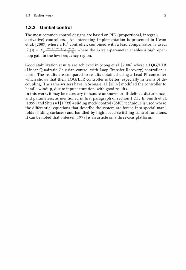
The most common control designs are based on PID (proportional, integral,derivative) controllers. An interesting implementation is presented in Kwonet al. [2007] where a PI2 controller, combined with a lead compensator, is used:Gs(s) = Kp
(s+ω1)(s+ω2)s2
a (s+ω3)(s+ω4) where the extra I-parameter enables a high open-
loop gain in the low frequency region.
Good stabilization results are achieved in Seong et al. [2006] where a LQG/LTR(Linear Quadratic Gaussian control with Loop Transfer Recovery) controller isused. The results are compared to results obtained using a Lead-PI controllerwhich shows that their LQG/LTR controller is better, especially in terms of de-coupling. The same writers have in Seong et al. [2007] modified the controller tohandle windup, due to input saturation, with good results.In this work, it may be necessary to handle unknown or ill-defined disturbancesand parameters, as mentioned in first paragraph of section 1.2.1. In Smith et al.[1999] and Shtessel [1999] a sliding mode control (SMC) technique is used wherethe differential equations that describe the system are forced into special mani-folds (sliding surfaces) and handled by high speed switching control functions.It can be noted that Shtessel [1999] is an article on a three-axis platform.


2Modelling
A mathematical model of the gimbal is important to deriving control strategies.It is for instance very difficult to tune PID parameters directly on a real systemwithout some knowledge about it. A common approach is to use step responsesand base the parameters on these. However, tests on a physical system are oftencomplicated and time consuming, especially when the system is nonlinear whichdemands tests in several linearization points. A simulation model environmentmakes the control design process easier and faster. There are also some modelbased control strategies where the model itself is a part of the control loop.
A model of the system is also important for correct interpretation of the sensorinputs.
The modelling of the gimbal is divided into kinematics and dynamics. The kine-matics will be used to interpret the sensors and will also be a part of the dynamicswhich in turn will be used in a simulation model.
2.1 Gimbal Properties
This section is a presentation of the gimbal properties without going into muchdetails.
2.1.1 Mechanics
The gimbal was mainly made of aluminium profiles and consisted of four bodies(body (0)-(3) in Figure 2.1 and 2.2) connected by three revolute joints. Each jointwas driven by a dc-motor (not shown in the figures below) via a gearbox. Themounting point of the camera on body (3) in the θ2 direction. The box on body(1) containded the electronics including the control card.
7

8 2 Modelling
Body (0) was supposed to be attached to the platform via a dampening jointwhich was supposed to cancel out some of the disturbances, e.g. from wind andmotor vibrations. However, the gimbal was not attached to a platform duringthis thesis so body (0) became the part of the gimbal which was held by hand orfixed during tests.
The dimensions (l1, h1, b2 and h3) in Figure 2.1 and 2.2, and the mass, mass mo-ment of inertia and center of mass for each body were given by the CAD modelsof the gimbal.
Figure 2.1: The gimbal in configuration θ = (0, 0, 0) viewed from the sidewith coordinate axes and distances between them. The direction of the jointsis indicated by the double arrows.
2.1 Gimbal Properties 9
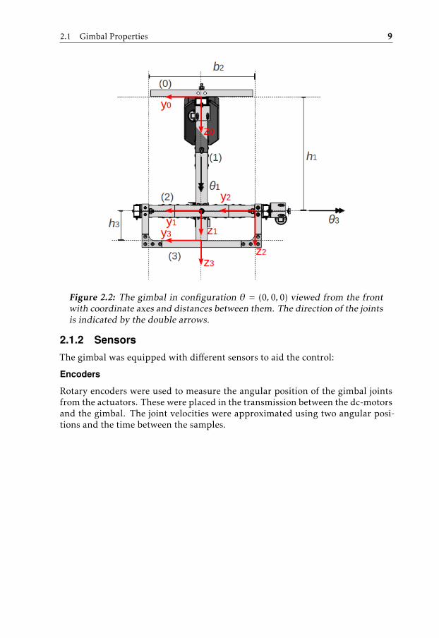
Figure 2.2: The gimbal in configuration θ = (0, 0, 0) viewed from the frontwith coordinate axes and distances between them. The direction of the jointsis indicated by the double arrows.
2.1.2 Sensors
The gimbal was equipped with different sensors to aid the control:
Encoders
Rotary encoders were used to measure the angular position of the gimbal jointsfrom the actuators. These were placed in the transmission between the dc-motorsand the gimbal. The joint velocities were approximated using two angular posi-tions and the time between the samples.

10 2 Modelling
IMU
The gimbal was equipped with an Inertial Measurement Unit (IMU) close to thecamera mounting point (origin of coordinate frame (3) in Figure 2.1). An IMUconsists of gyroscopes (gyros) and accelerometers measuring accelerations andchanges in attitude such as roll, pitch and yaw. The unit can with this infor-mation calculate the angular velocity of the device it is mounted on. The gyros(gyroscopes) were used to measure the angular velocities of the camera and thesevelocities were integrated to calculate the camera’s angular position relative tothe ground (attitude). However, a simple integration of the calculated velocities("dead reckoning") also leads to accumulation of the errors present in them. Theaccumulated errors creates an ever-increasing difference between the calculatedattitude and the actual attitude (drift). The drift is usually corrected using othersensors such as a GPS, which not available. A filter solution from IA using ac-celerometer data was used to get more correct attitudes (section 3.2.2).
2.1.3 User Input
User input to the gimbal consisted of two modes with either the desired angularvelocities, or the desired attitude.
The first of these control modes was supposed to be used when the photographeruses a hand controller to control the yaw, pitch and roll of the camera in referenceto its image output, i.e. the velocities are first defined in the camera’s coordinateframe. The input from the hand controller consists three values that are inter-preted as desired angular velocities of the camera. The gimbal control unit thencalculates new reference velocities of the gimbal joints. When input ceases, sodoes the change in attitude.
The second input mode was a desired angular position relative to the ground(attitude). These angles are transformed to the gimbal’s reference frames usingthe information from the IMU and new reference joint angles are given to thecontrol.

2.2 Kinematics 11
2.2 Kinematics
The kinematics of a mechanical system is, according to Jazar [2007], the descrip-tion of the system’s translational and angular position and their time derivativestaking only geometry into account. The forces that cause the motion of the systemare not taken into consideration but the kinematics can be used in the derivationof the dynamics of the system (section 2.3) which take into account all forces act-ing upon it. The basics of the kinematics of a rigid multi body system (MBS) is todescribe the motion of a body in a coordinate frame attached in another body (e.g.a global fixed reference frame) using matrix algebra. The approach to do this isto combine a series of individual transformations between the body-attached co-ordinate systems. These transformations are a description of the relative rotationand distance between the bodies and consist of variable parameters according tothe degrees of freedom (DOF) between the bodies. The gimbal in this thesis (seeFigures 2.1 and 2.2) consists only of three revolute joints (R-joints) that individ-ually have only one DOF (see Figure 2.3). This gives the whole MBS a total ofthree DOF, yaw, roll and pitch (θ1, θ2, θ3). These are the joint parameters thathenceforth will be used to describe the system. The kinematics can be dividedinto forward and inverse kinematics.
(B)
(A)
θB
θB
Figure 2.3: Principal sketch of a revolute joint (R-joint) with index [B] wherebody (B) is rotated an angle indicated by the joint parameter θB. It has inthis case its zero value on the axis orthogonal to the length of body (A). θBindicates the direction of the joint (the thumb in the right-hand-rule). A R-joint has only one degree of freedom and therefore only one joint parameter.

12 2 Modelling
2.2.1 Forward Kinematics
Forward kinematics of an MBS is how the configuration of the joint parametersaffects the translational and angular position of an end effector. In robotics, theend effector is often the point where the robot’s tools are attached and the "tool"of the gimbal was a camera. The forward kinematics can be described by transfor-mation matrices. Serial robots are often described using the Denavit-Hartenbergmethod Jazar [2007][p. 199] which uses a sets of rules to systematically derive theforward kinematics in a standardized form. This method places the coordinatesystems of each body according to the directions of the joints, for instance thez-axis parallel to the joint direction θ. However, since these coordinate systemsand joint parameters seemed counterintuitive for this application, the methodwas abandoned in favour of for a more traditional rigid body mechanics methodwhere the coordinate systems in the bodies are placed more freely.
Relation between axes and joint parameters
In Figures 2.1 and 2.2 there are two types of axes: the coordinate axes (xi , yi , zi),indicated by an one-headed arrow, and the joint parameter axes (θ1, θ2, θ3), indi-cated by the double-headed arrows. The joint parameters describe the angularposition of the three joints in the gimbal, according to Figure 2.3. For the wholegimbal, motions in these joints are called yaw (θ1), roll (θ2) and pitch (θ3). Ac-cording to a common flight convention (Jazar [2007][p. 41]) yaw, roll, and pitchare defined such that yaw is a motion around a body’s z-axis, roll around its x-axis and pitch around its y-axis. Each body can only move in one DOF so the jointparameters are defined in the following way: θ1 as body (1)’s motion around thez0-axis (yaw), θ2 as body (2)’s motion around the x1-axis (roll) and θ3 as body(3)’s motion around the y2-axis (pitch). The coordinate systems in the bodies ofthe gimbal (Figures 2.1 and 2.2) are placed in a way that they are parallel to eachother in the configuration (θ1, θ2, θ3) = (0, 0, 0). The forward kinematic matricesderived in this section are used in the dynamic modelling in section 2.3 as wellas in the inverse kinematics described in section 2.2.2.
Homogeneous Transformations
The coordinate of an arbitrary point P of a rigid body in a local coordinate frameB is in this thesis denoted as the coordinate vector BrP . The point can be de-scribed in a different coordinate frame G using the rotation matrix GRB and thetranslation vector GdB between the frames.
GrP = GRBBrP +G dB, (2.1)
where in a 3D environment
BrP =
BxPByPBzP
. (2.2)
The expression (2.1) is called the transformation of the coordinate P from frameB to frame G.

2.2 Kinematics 13
It is often required to do several intermediate transformations to get the finaltransformation between two frames:
2.1 ExampleThe transformation between frame B2 and frame B0 is described by
0r = 0R22r + 0d2, (2.3)
where the components can be described using an intermediate coordinate frameB1
0R2 = 0R11R2 (2.4)
0d2 = 0R11d2 + 0d1. (2.5)
The expressions for the transformations get very messy even if with relativelyfew intermediate frames. A convenient way to describe a transformation is to usehomogeneous transformation matrices GTB, where for a 3D environment
GTB =[GRB
GdB01×3 1
]. (2.6)
The coordinate vector Br that is being transformed must also be in a homogeneousform
Bhr =
[Br1
]. (2.7)
2.2 ExampleThe transformation between frame B2 and frame B0 is described by
0hr = 0T2
2hr, (2.8)
where
0hr =
[0r1
], 2
hr =[
2r1
](2.9)
and0T2 = 0T1
1T2. (2.10)
14 2 Modelling
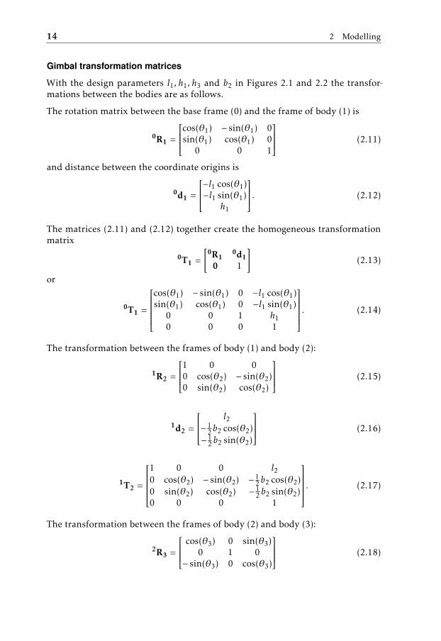
Gimbal transformation matrices
With the design parameters l1, h1, h3 and b2 in Figures 2.1 and 2.2 the transfor-mations between the bodies are as follows.
The rotation matrix between the base frame (0) and the frame of body (1) is
0R1 =
cos(θ1) − sin(θ1) 0sin(θ1) cos(θ1) 0
0 0 1
(2.11)
and distance between the coordinate origins is
0d1 =
−l1 cos(θ1)−l1 sin(θ1)
h1
. (2.12)
The matrices (2.11) and (2.12) together create the homogeneous transformationmatrix
0T1 =[
0R10d1
0 1
](2.13)
or
0T1 =
cos(θ1) − sin(θ1) 0 −l1 cos(θ1)sin(θ1) cos(θ1) 0 −l1 sin(θ1)
0 0 1 h10 0 0 1
. (2.14)
The transformation between the frames of body (1) and body (2):
1R2 =
1 0 00 cos(θ2) − sin(θ2)0 sin(θ2) cos(θ2)
(2.15)
1d2 =
l2−1
2b2 cos(θ2)−1
2b2 sin(θ2)
(2.16)
1T2 =
1 0 0 l20 cos(θ2) − sin(θ2) −1
2b2 cos(θ2)0 sin(θ2) cos(θ2) −1
2b2 sin(θ2)0 0 0 1
. (2.17)
The transformation between the frames of body (2) and body (3):
2R3 =
cos(θ3) 0 sin(θ3)0 1 0
− sin(θ3) 0 cos(θ3)
(2.18)

2.2 Kinematics 15
2d3 =
h3 sin(θ3)12b2
h3 cos(θ3)
(2.19)
2T3 =
cos(θ3) 0 sin(θ3) h3 sin(θ3)
0 1 0 12b2
− sin(θ3) 0 cos(θ3) h3 cos(θ3)0 0 0 1
. (2.20)
The total transformation between body (3) and the base is
0T3 =[
0R30d3
0 1
]= 0T1
1T22T3, (2.21)
where, with the notation ci = cos(θi) and si = sin(θi),
0R3 =
c1c3 − s1s2s3 −c2s1 c1s3 + c3s1s2c3s1 + c1s2s3 c1c2 s1s3 − c1c3s2−c2s3 s2 c2c3
(2.22)
and
0d3 =
c1l2 − c1l1 + c1h3s3 + c3h3s1s2l2s1 − l1s1 + h3s1s3 − c1c3h3s2
h1 + c2c3h3
. (2.23)
0R3 is a pitch-roll-yaw rotation matrix. It can also more generally be called aZXY triple rotation matrix Jazar [2007][p. 40] due to the order in which the ro-tation matrices are successively multiplied. These transformations are used inthe derivation of the inverse kinematics in section 2.2.2 as well as the dynamics insection 2.3.
One other transformation that is used in the Inverse kinematics in section 2.2.2is the rotation between body (3) and the ground, viewed as an imaginary bodycalled (g). The angular position of body (3) is derived using the informationfrom the gyros and accelerometers on the IMU attached to the body which arerepresented by a pitch-roll-yaw matrix, similar to matrix (2.22).
gR3 =
cα1cα3 − sα1sα2sα3 −cα2sα1 cα1sα3 + cα3sα1sα2cα3sα1 + cα1sα2sα3 cα1cα2 sα1sα3 − cα1cα3sα2
−cα2sα3 sα2 cα2cα3
, (2.24)
where sαi and cαi are short for sin(αi) and cos(αi) and α1 = yaw, α2 = roll andα3 = pitch derived using the information from the IMU. There exist a total of12 possible independent orientation representation of this type, but this one waschosen due to its similarity to matrix (2.22).

16 2 Modelling
2.2.2 Inverse Kinematics
The opposite of forward kinematics is when the joint parameters are determinedfrom the translational and angular position of the end-effector. This is called in-verse kinematics. In a common robotic application the goal is to move a tool toa certain position and hold it in a certain orientation. This is often a difficultproblem because it leads to multiple solutions which are often avoided by lettingthe robot "learn" the configuration of the joint parameters instead of computingthem. Inverse kinematics in the gimbal application is simpler, because in thiscase it is only concerned with the orientation (in this thesis called angular posi-tion) of the camera. Thus multiple solutions of trigonometric functions can beavoided. The inverse kinematics will be used to generate the reference signals tothe gimbal control.
Angular position
According to the second user input mode described in section 2.1.3 one goal isto change the attitude of the camera relative to the ground. This will result ina control error between the desired attitude and with gyros and accelerometersderived current attitude described by (2.24). This can be presented as a newrotation matrix in the camera’s reference frame.
3Re =
cε1cε3 − sε1sε2sε3 −cε2sε1 cε1sε3 + cε3sε1sε2cε3sε1 + cε1sε2sε3 cε1cε2 sε1sε3 − cε1cε3sε2
−cε2sε3 sε2 cε2cε3
, (2.25)
where ε1, ε2 and ε3 are the errors (ε = αdes − α) of yaw, roll and pitch in thecamera’s reference frame. e denotes an imagined error coordinate frame.
The total rotation matrix between the error frame (e) and the gimbal base frame(0) is then
0Re(Θ, ε) = 0R3(Θ) 3Re(ε), (2.26)
where Θ are the current angles of the joints (θ1, θ2, θ3) (Figures 2.1, 2.2 and 2.3).
A new joint configuration Θnew is chosen such that0R3(Θnew) = 0Re(Θ, ε), (2.27)
which means that coordinate frame (3) becomes in the same frame as (e), i.e thedesired attitude is reached.

2.2 Kinematics 17
Equation (2.27) gives together with (2.26)0R3(Θnew =0 R3(Θ) 3Re. (2.28)
If the right hand side of (2.28) is expressed as
0R3(Θ) 3Re =
r11 r12 r13r21 r22 r23r31 r32 r31
, (2.29)
where rij is the matrix component ij of 0R3(Θ) 3Re, then (2.28) together with(2.22), in section 2.2.1, gives the new joint parameters:
θ1new = arctan2(−r12, r22), (2.30a)
θ2new = arcsin(r32), (2.30b)
θ3new = arctan2(−r31, r33), (2.30c)
where arctan2(y,x) is a function that places the computed angle in the correctquadrant of the unit circle.
These angles will be the angular position reference signals for the individualjoints.
Angular velocity
According to the first user input mode described in section 2.1.3, the input canbe a set of desired angular velocities Φ of the camera in its own coordinate frame:
33Φ =
ϕxϕyϕz
=
ϕrollϕpitchϕyaw
. (2.31)
The relationship between the local angular velocitiesΩ in the joints and the cam-era angular velocity can be expressed using a Jacobian matrix J
33Φ = JΩ, (2.32)
where
Ω = (ω1, ω2, ω3)T = (θ1, θ2, θ3)T . (2.33)

18 2 Modelling
As in Jazar [2007][p. 351] the Jacobian J can be viewed as the angular velocitydirections of the joints presented in the camera’s coordinate frame and becausethe gimbal consists only of R-joints it can be written as
J =[3θ1
3θ23θ3
]=
[3R1
1θ13R2
2θ23θ3
]=
[(1R2
2R3
)T 1θ12RT
32θ2
3θ3
], (2.34)
where
1θ1 =
001
, 2θ2 =
100
, 3θ3 =
010
, (2.35)
which are the directions of the joints (Figures 2.1, 2.2 and 2.3).
(2.32) is then ϕrollϕpitchϕyaw
=
− cos(θ2) sin(θ3) cos(θ3) 0sin(θ2) 0 1
cos(θ2) cos(θ3) sin(θ3) 0
ω1ω2ω3
, (2.36)
which is then reordered to ϕyawϕrollϕpitch
=
cos(θ2) cos(θ3) sin(θ3) 0− cos(θ2) sin(θ3) cos(θ3) 0
sin(θ2) 0 1
ω1ω2ω3
. (2.37)
The desired joint velocities Ω can then be expressed as
Ω = J−1
ϕyawϕpitchϕroll
. (2.38)
It is also possible to derive the current translational velocity X of the end-effectorwith another Jacobian matrix Jd
X = JDΩ =[3θ0 × 3d1
3θ1 × 3d23θ2 × 3d3
]Ω. (2.39)
This can be useful if the translational velocity is needed, e.g. in applications suchas positional tracking and sensor filtering. Translational Jacobians are used in thedynamics in section 2.3.

2.3 Dynamics 19
2.3 Dynamics
The dynamics of an MBS is how its motion is affected by external forces such asgravity and torque from the joint actuators. It is presented as a system of differen-tial equations obtained using either Newton-Euler equations Jazar [2007][p. 447],which use Newton’s second law of motion, or Lagrange equationsJazar [2007][p. 478], which uses the kinetic and potential energies of the MBS.The method using Lagrange equations was chosen in this thesis. The reason forthis is mainly the writer’s desire to learn this method.
2.3.1 Lagrange Dynamics
A systematic way to obtain the equations of motion of a robot with n joints isaccording to Jazar [2007][p. 528] to use the Lagrange equation:
ddt
(∂L∂ωi
)− ∂L∂θi
= Qi i = 1, 2, . . . n. (2.40)
L is the Lagrangian which is defined as the difference between the kinetic energyK and potential energy V
L = K − V . (2.41)
θi are the coordinates of the system (which in the gimbal application are thecurrent angles in joints i = 1, 2, 3). ωi is the time derivative θi of the coordi-nates and Qi is the non-potential force driving θi . Qi are external forces such astorques from actuators while internal forces such as gravity and Coriolis effectsJazar [2007][p. 451] are already a part of the left hand side of equation (2.40).
According to the proof in Jazar [2007][p. 529] the kinetic energy of the wholerobot can be expressed as
K =12ΩTj DΩj j = 1, 2, . . . n, (2.42)
where Ω = (ω1, ω1, ω3)T and D is the n × n matrix
D =n∑j=1
(JTDj mj JDj +
12
JTRj0Ij JRj
), (2.43)
which is called the inertial-type matrix. JDj and JRj are the Jacobians of body (j)that transform the joint angular velocities into the translational and rotationalvelocities of the body’s center of mass (CM) (similar to the jacobians in section2.2.2). The component mj is the mass of body (j) and 0Ij is the Mass moment ofinertia matrix about its CM and expressed in the base coordinate frame (0).

20 2 Modelling
The potential energy can according to the same proof [Jazar, 2007, p. 529] bewritten as
V =n∑i=1
Vi = −n∑i=1
mi0gT 0ri , (2.44)
where 0g is the gravitational acceleration vector in the base frame (0) and 0ri arethe coordinates of the center of mass of each body expressed in the base frame(0).
If equations (2.41) to (2.44) are inserted in (2.40) the result can with some rear-rangement (done in Jazar [2007][p. 529]) and Θ = (θ1, θ2, θ3)T be presented in amatrix form
D(Θ)Ω+ H(Θ,Ω) + G(Θ) = Q, (2.45)
or in summation formn∑j=1
Dij (θ)ωj +n∑k=1
n∑l=1
Hiklωkωl + Gi = Qi . (2.46)
The index i = 1, 2, . . . n indicates the row of the equation.
Vector H is called the Velocity coupling vector and is
Hi =n∑k=1
n∑l=1
Hijkωkωl
= Hi11ω1ω1 + . . . + Hin1ωnω1 + . . . + Hinnωnωn, (2.47)
(2.48)
where
Hijk =n∑j=1
n∑k=1
(∂Dij∂θk
− 12
∂Djk∂θi
). (2.49)
The last term in (2.46) is the Gravitational vector Gi
Gi =n∑j=1
mj0gT J(i)
Dj . (2.50)
Equation (2.46) can in theory be viewed as how reaction torques Q in each jointare affected. The n × n inertial-type matrix D is how the reaction torques areaffected by a given set of accelerations Ω due to the inertias of the bodies andevery component outside the diagonal are coupling effects. The n × 1 Velocitycoupling vector H contains the reactions due to a given set of angular velocitiesΩ and the bodies’ inertias and coupling effects. H can often be referred as aChristoffel operator Jazar [2007][p. 533]. The n × 1 Gravitational vector G containsthe reaction torques in the joints due to the gravitational pull 0g.
2.3 Dynamics 21
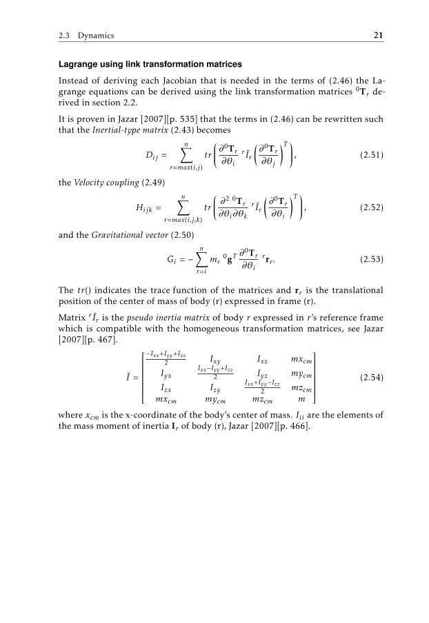
Lagrange using link transformation matrices
Instead of deriving each Jacobian that is needed in the terms of (2.46) the La-grange equations can be derived using the link transformation matrices 0Tr de-rived in section 2.2.
It is proven in Jazar [2007][p. 535] that the terms in (2.46) can be rewritten suchthat the Inertial-type matrix (2.43) becomes
Dij =n∑
r=max(i,j)
tr
∂0Tr∂θi
r Ir
(∂0Tr∂θj
)T , (2.51)
the Velocity coupling (2.49)
Hijk =n∑
r=max(i,j,k)
tr
∂2 0Tr∂θi∂θk
r Ir
(∂0Tr∂θi
)T , (2.52)
and the Gravitational vector (2.50)
Gi = −n∑r=i
mr0gT
∂0Tr∂θi
rrr . (2.53)
The tr() indicates the trace function of the matrices and rr is the translationalposition of the center of mass of body (r) expressed in frame (r).
Matrix r Ir is the pseudo inertia matrix of body r expressed in r’s reference framewhich is compatible with the homogeneous transformation matrices, see Jazar[2007][p. 467].
I =
−Ixx+Iyy+Izz
2 Ixy Ixz mxcmIyx
Ixx−Iyy+Izz2 Iyz mycm
Izx IzyIxx+Iyy−Izz
2 mzcmmxcm mycm mzcm m
(2.54)
where xcm is the x-coordinate of the body’s center of mass. Iii are the elements ofthe mass moment of inertia Ir of body (r), Jazar [2007][p. 466].

22 2 Modelling
2.3.2 Dynamics of the gimbal
One difference between the gimbal application and most robotic applications isthe gravitational vector 0g. The direction of it is in most applications constantstraight down (along the global z-axis). The gimbal is however supposed to be inflight which means that 0g varies with the attitude of platform. The gravitationalvector (0, 0, g)T on the ground is therefore transformed to the base frame (0) viagyro and accelerometer data from the IMU.
0g = 0R3gRT
3
00g
= 0R3
−cα2sα3sα2
cα2cα3
g (2.55)
where 0R3 is (2.22), gRT3 the inverse of (2.24) and g is the gravitational accelera-
tion (9.81m/s2). This gives that G in (2.45) becomes a function of both the jointparameters Θ and the IMU attitude α, G(Θ, α).
With the aid of Matlab symbolic toolbox and Mathematica, the terms D(Θ)Ω,H(Θ,Ω) and G(Θ, α) were obtained using the kinematics in section 2.2. The de-sign parameters described in section 2.1, such as masses, lengths and momentsof inertia I were taken from the CAD-models of the gimbal.
The Lagrange equations (2.45) were rearranged to
Ω = D−1(Q −H −G) (2.56)
and a state vector was defined to describe the dynamics
x =[Ω
Θ
]=
ω1ω2ω3θ1θ2θ3
. (2.57)
With (2.56) and one derivation of (2.57) the system of differential equations thatdescribes the dynamics of the gimbal were obtained
x =[D(x4:6)−1(Q −H(x) −G(x4:6, α))
x1:3
]. (2.58)
The IMU attitude α could have been a set of states among (2.57) but is not directlya part of the joint states and is therefore viewed as a separate set of states.

2.3 Dynamics 23
Camera mechanics
A camera attached to the gimbal is in the dynamic calculations viewed as a partof body (3), Figure 2.1. If the camera is changed the mass m3, center of masscoordinates 3r3 and the mass moment of inertia I3 of body (3) will also change.The new mass of the body is simply the addition of the masses of the camera andthe original body:
m3 = m3org + mc. (2.59)
According to Jazar [2007][p. 449] the combined center of mass of a rigid body Bis defined as
Brcm =1m
∫B
r dm. (2.60)
If the masses mi and the center of masses ri = (xcm, ycm, zcm)T are known for eachpart of the body, equation (2.60) can be written as
Brcm =1∑mi
∑rimi , (2.61)
where the summations are of each body (i) incuded in body B.
In the gimbal application the center of mass of body (3) with a camera attachedbecomes
3r3 =1m3
(r3orgm3org + rcmc). (2.62)
Vector r3org is the coordinate of the original body’s center of mass expressed inthe coordinate frame (3) (see Figure 2.2) and rc is the center of mass of the cameraexpressed in coordinate frame (3).
The total mass moment of inertia of body (3) is obtained using the parallel-axestheorem, also called Huygens-Steiner’s theorem (Jazar [2007][p. 473]).
I3 = I3org + m3org r3org rT3org + Ic + mc rc rTc , (2.63)
where
ri =
0 −zcm ycmzcm 0 −xcm−ycm xcm 0
. (2.64)
ri is the skew-symmetric matrix form of ri .
The shape of the camera can be simplified to be a cuboid and the mass momentof inertia can be looked up in a table of moments of inertias. If a camera objectiveis used the total camera properties can be calculated as in equations (2.59), (2.62)and (2.63).

24 2 Modelling
The same theory can be applied if other parts of the gimbal are not included inthe original body. It can for instance be useful to treat the motors of the gim-bal as separate bodies if simulation tests of different actuators (motors and gear-boxes) are desired. Instead of generating a whole new model, with a differentset of actuators or a different camera, their mechanical properties are treated assymbolic quantities, and given appropriate values in the simulation environment.The model in this thesis allows for interchangeable cameras, but not actuators, asthese are included in the original gimbal bodies.
Friction
The torques Q on the gimbal are affected by friction which is assumed to be linear
Q = τa − τ f sgn(Ω) − µΩ (2.65)
where τa are the torques from the actuators, τf the static frictions in the jointsand µ is a diagonal matrix containing the kinetic friction coefficients of the joints.
The combined torques in a joint need in reality overcome the static friction τfin order to create a motion. The condition for the gimbal to behave according to(2.58) from a standstill is therefore according to Algorithm 2.1.
Algorithm 2.1 Condition for motion in joint i due to static friction
if(∣∣∣∣[τa −DΩ−H −G)
]i
∣∣∣∣ < τf (i))
&& (ωi == 0) then
ωi = 0;else
ωi =[D−1(Q −H −G)
]i;
end if
Actuator dynamics
According to Mohan et al. [2003] dc-motor drives can be described using thefollowing equations:
τm = Kt i, (2.66)
where τm is the output torque from the motors, Kt the torque constant and i thecurrent. The current is expressed in the differential equation
didt
=1L
(u − Rmi − e), (2.67)
where u is the input voltage, Rm the resistance of the motor circuit, e the back-emfof the motor and L the motors inductance. e is produced by the angular velocityωm
e = Keωm, (2.68)
where Ke the back-emf constant.
2.4 Identification 25
With the coupling ratio a = ωmω = τa
τmof the gearboxes the equations of the actua-
tors becomes
τa = Ktai (2.69)
anddidt
=1L
(u − Rmi − Keaω) (2.70)
The constants Kt , Ke L, Rm and a are taken from the data sheets of the motor andthe gearbox.
2.4 Identification
If the data from the CAD-models, mentioned in section 2.3.2, is assumed to becorrect, the only unknown parameters in equations (2.58) to (2.70) that need tobe estimated are the friction parameters τf and µ for each axis. The noise in thegimbal’s sensors was identified in this section and was later added as disturbancein the simulation environment.
2.4.1 Friction tuning
In order to estimate the friction in each axis a series of voltage step responsetests were made. The results from these tests were compared to the results fromthe same steps in the simulation environment. The static and dynamic frictionparameters in the model, τf and µ mentioned in section 2.3.2, were then simplytuned to get a simulation result that fitted the results from the real measurements.All tests were done around θ = (0, 0, 0).
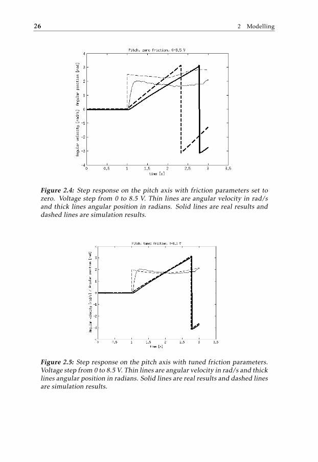
Figure 2.4 shows that the simulation results were quite close to the real measure-ments but the overall angular velocity was too high. The static friction parameterτf was tuned to reduce the overall angular velocity and the dynamic friction pa-rameter µ was tuned to set a penalty on higher angular velocities. The result isshown in Figure 2.5.
26 2 Modelling
Figure 2.4: Step response on the pitch axis with friction parameters set tozero. Voltage step from 0 to 8.5 V. Thin lines are angular velocity in rad/sand thick lines angular position in radians. Solid lines are real results anddashed lines are simulation results.
Figure 2.5: Step response on the pitch axis with tuned friction parameters.Voltage step from 0 to 8.5 V. Thin lines are angular velocity in rad/s and thicklines angular position in radians. Solid lines are real results and dashed linesare simulation results.

2.4 Identification 27
The behaviour was somewhat different when the voltage to the motors were re-versed, as shown in Figure 2.6. Negative directions of the torque on the axesneeded separate sets of friction parameters. The results of friction tuning in thenegative direction on the pitch axis is shown in Figure 2.7.
Figure 2.6: Negative step response on the pitch axis with same friction pa-rameters as the positive step. Voltage step from 0 to -8.5 V. Thin lines areangular velocity in rad/s and thick lines angular position in radians. Solidlines are real results and dashed lines are simulation results.
Figure 2.7: Negative step response on the pitch axis with tuned friction pa-rameters. Voltage step from 0 to -8.5 V. Thin lines are angular velocity inrad/s and thick lines angular position in radians. Solid lines are real resultsand dashed lines are simulation results.

28 2 Modelling
The results from the roll and yaw axes are shown in Figure 2.8 to 2.13.
Figure 2.8: Step response on the roll axis with friction parameters set tozero. Voltage step from 5.1 to 17 V. Thin lines are angular velocity in rad/sand thick lines angular position in radians. Solid lines are real results anddashed lines are simulation results.
Figure 2.9: Step response on the roll axis with with tuned friction parame-ters. Voltage step from 5.1 to 17 V. Thin lines are angular velocity in rad/sand thick lines angular position in radians. Solid lines are real results anddashed lines are simulation results.
2.4 Identification 29
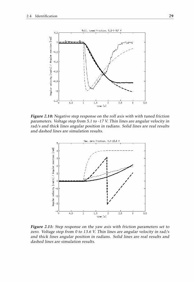
Figure 2.10: Negative step response on the roll axis with with tuned frictionparameters. Voltage step from 5.1 to -17 V. Thin lines are angular velocity inrad/s and thick lines angular position in radians. Solid lines are real resultsand dashed lines are simulation results.
Figure 2.11: Step response on the yaw axis with friction parameters set tozero. Voltage step from 0 to 13.6 V. Thin lines are angular velocity in rad/sand thick lines angular position in radians. Solid lines are real results anddashed lines are simulation results.

30 2 Modelling
Figure 2.12: Step response on the yaw axis with tuned friction parameters.Voltage step from 0 to 13.6 V. Thin lines are angular velocity in rad/s andthick lines angular position in radians. Solid lines are real results and dashedlines are simulation results.
Figure 2.13: Negative step response on the yaw axis with tuned friction pa-rameters. Voltage step from 0 to -13.6 V. Thin lines are angular velocity inrad/s and thick lines angular position in radians. Solid lines are real resultsand dashed lines are simulation results.
2.4 Identification 31
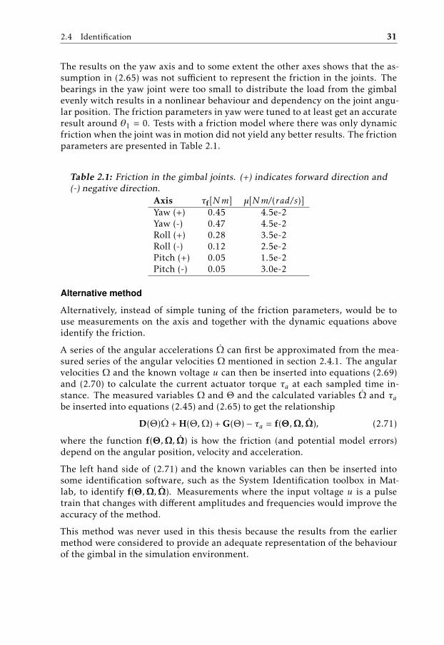
The results on the yaw axis and to some extent the other axes shows that the as-sumption in (2.65) was not sufficient to represent the friction in the joints. Thebearings in the yaw joint were too small to distribute the load from the gimbalevenly witch results in a nonlinear behaviour and dependency on the joint angu-lar position. The friction parameters in yaw were tuned to at least get an accurateresult around θ1 = 0. Tests with a friction model where there was only dynamicfriction when the joint was in motion did not yield any better results. The frictionparameters are presented in Table 2.1.
Table 2.1: Friction in the gimbal joints. (+) indicates forward direction and(-) negative direction.
Axis τf[Nm] µ[Nm/(rad/s)]Yaw (+) 0.45 4.5e-2Yaw (-) 0.47 4.5e-2Roll (+) 0.28 3.5e-2Roll (-) 0.12 2.5e-2Pitch (+) 0.05 1.5e-2Pitch (-) 0.05 3.0e-2
Alternative method
Alternatively, instead of simple tuning of the friction parameters, would be touse measurements on the axis and together with the dynamic equations aboveidentify the friction.
A series of the angular accelerations Ω can first be approximated from the mea-sured series of the angular velocities Ωmentioned in section 2.4.1. The angularvelocities Ω and the known voltage u can then be inserted into equations (2.69)and (2.70) to calculate the current actuator torque τa at each sampled time in-stance. The measured variables Ω and Θ and the calculated variables Ω and τabe inserted into equations (2.45) and (2.65) to get the relationship
D(Θ)Ω+ H(Θ,Ω) + G(Θ) − τa = f(Θ,Ω, Ω), (2.71)
where the function f(Θ,Ω, Ω) is how the friction (and potential model errors)depend on the angular position, velocity and acceleration.
The left hand side of (2.71) and the known variables can then be inserted intosome identification software, such as the System Identification toolbox in Mat-lab, to identify f(Θ,Ω, Ω). Measurements where the input voltage u is a pulsetrain that changes with different amplitudes and frequencies would improve theaccuracy of the method.
This method was never used in this thesis because the results from the earliermethod were considered to provide an adequate representation of the behaviourof the gimbal in the simulation environment.

32 2 Modelling
2.4.2 Sensor noise
Sensor noise was added to the model as sets of variances taken from the measure-ments in Figures 2.14 to 2.17 there the gimbal was held in a fixed configuration.
Figure 2.14: Noise from an encoder measurement after filtering in the gim-bal controller. The signal with small variance is the angular position of theencoder and the signal with much bigger variance is the angular velocitywhich is the filtered derivative of the angular position.
Figure 2.15: Measurement of the noise in the yaw magnetometer in the IMUwhen the gimbal was held stationary.
2.4 Identification 33
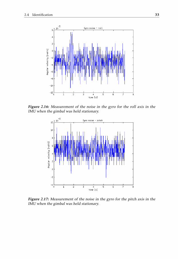
Figure 2.16: Measurement of the noise in the gyro for the roll axis in theIMU when the gimbal was held stationary.
Figure 2.17: Measurement of the noise in the gyro for the pitch axis in theIMU when the gimbal was held stationary.

34 2 Modelling
It is shown in figure 2.14 that the angular position noise is mainly due to the lastsampled bit in in the signal from the encoder. The real value was somewherebetween the value when the least significant bit in the binary signal was 1 or thevalue when the bit was 0 and the signal jumped between these values. The angu-lar velocity was simply a derivative of the angular position. As a simplificationthe noise was modelled as white noise with bias and variance according to table2.2. The noise of the angular position and velocities was also simplified to beviewed as independent.
The largest part of the angular velocity bias was compensated for using the mea-surements of the IMU. However, a small bias remains after compensation Thebiases and variances are presented in table 2.2.
The noise on the sensor signals was relatively small due to filtering and bias com-pensations present in the gimbal controller and can in most cases be disregarded,see section 3.1.
Table 2.2: Bias and variances of the noise in the encoders and the IMU.Signal Bias [rad(/s)] Variance [(rad(/s))2]Encoder angular position -5.5632e-04 1.2617e-06Encoder angular velocity -4.5697e-03 4.5971e-04Magnetometer yaw 6.7044e-04 4.1017e-06Gyro roll -3.1824e-03 5.9804e-06Gyro pitch 4.9598e-03 4.0390e-06

3Implementation and control
When the modelling described in chapter 2 was done, a simulation environmentwas constructed. This simulation environment was then used as a tool in devel-opment of the gimbal control structure for the gimbal in the simulation environ-ment and in the gimbal hardware.
3.1 Simulation
The model obtained in section 2.3 was included as in Figure 3.1 in a control struc-ture shown in appendix A. Due to the much too weak motors, the "camera" re-ferred to below can be considered a weightless object mounted on body (3) inFigure 2.1.
3.1.1 Dynamics in Simulink
The dynamic model of the gimbal is set up as a Simulink model (Figure 3.1)
Figure 3.1: Dynamics of the gimbal presented in Simulink.
35

36 3 Implementation and control
The block called gimbalmod is an S-function which contains the differential equa-tions (2.58) and the friction handling. The input is the current state vector x,the generated attitude angles to the ground α, the torque from the actuators τmand a check if the angular velocity has reached zero which is used in the frictionhandling. The output of the function is the derivative state x. The differentialequations are solved using an integrator and a solver such as ode45.
The motors block is set up according to Figure 3.2 and the differential equation ofthe current i is solved with an integrator.
Figure 3.2: Dynamics of the actuators presented in Simulink.
3.1.2 Control structure
The control structure shown in Figure A.1 in appendix A is a joint angular ve-locity and position controller in cascade with an output signal between -1 and 1.The output signal is then multiplied with the battery voltage input to the gimbalmotors. This is to get the same behaviour as a by pulse-width modulation (pwm)controlled voltage. There are also input signals for the desired angular positionsand velocities in the camera’s coordinate frame which are transformed to the jointframes. The last part of the structure in Figure A.1 is a model of how gyros closeto the camera would behave when the entire gimbal is disturbed. This structurecan be compared to the block diagram in Figure 3.14.
3.1 Simulation 37
Controllers
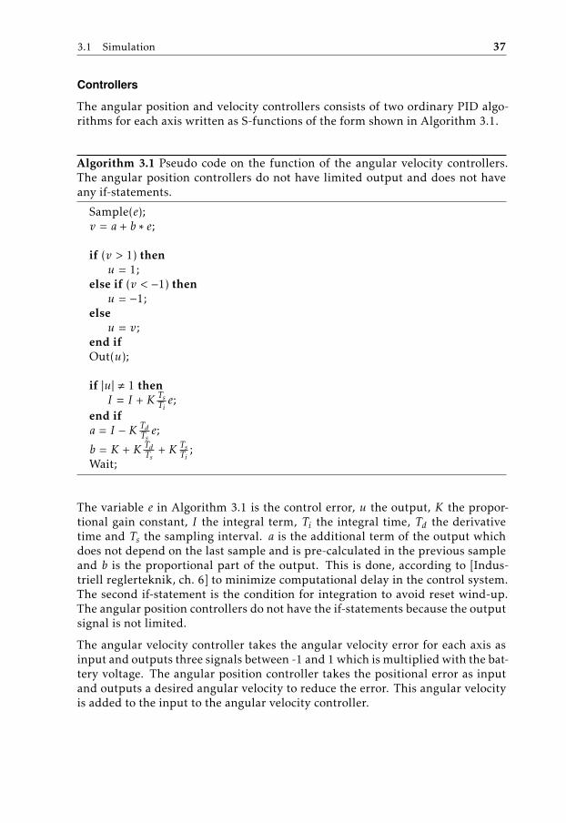
The angular position and velocity controllers consists of two ordinary PID algo-rithms for each axis written as S-functions of the form shown in Algorithm 3.1.
Algorithm 3.1 Pseudo code on the function of the angular velocity controllers.The angular position controllers do not have limited output and does not haveany if-statements.
Sample(e);v = a + b ∗ e;
if (v > 1) thenu = 1;
else if (v < −1) thenu = −1;
elseu = v;
end ifOut(u);
if |u| , 1 thenI = I + K Ts
Tie;
end ifa = I − K Td
Tse;
b = K + K TdTs
+ K TsTi
;Wait;
The variable e in Algorithm 3.1 is the control error, u the output, K the propor-tional gain constant, I the integral term, Ti the integral time, Td the derivativetime and Ts the sampling interval. a is the additional term of the output whichdoes not depend on the last sample and is pre-calculated in the previous sampleand b is the proportional part of the output. This is done, according to [Indus-triell reglerteknik, ch. 6] to minimize computational delay in the control system.The second if-statement is the condition for integration to avoid reset wind-up.The angular position controllers do not have the if-statements because the outputsignal is not limited.
The angular velocity controller takes the angular velocity error for each axis asinput and outputs three signals between -1 and 1 which is multiplied with the bat-tery voltage. The angular position controller takes the positional error as inputand outputs a desired angular velocity to reduce the error. This angular velocityis added to the input to the angular velocity controller.

38 3 Implementation and control
IMU
In order to disturb the simulation with a motion on the zero frame a block wasrequired that transformed a given angular velocity in zero frame to how the gy-roscopes on an IMU close to the camera would measure it. First the componentsof the angular velocity Φ0 were transformed to the joints. This can be viewed asif the joints themselves produce the motion ΩΦ and the zero frame is fixed.
ΩΦ = jointsJ0Φ0, (3.1)
where jointsJ0 is the Jacobian
jointsJ0 =
1 0 00 sin(θ1) cos(θ1)
sin(θ2) cos(θ1) cos(θ2) − cos(θ2) sin(θ1)
. (3.2)
Then, the angular velocities Ω, which are actually produced by the joints, areadded to ΩΦ. These are then transformed to the camera frame using equation(2.32). The angular velocity that the gyros on the IMU detects is then
33Φ = J(ΩΦ + Ω). (3.3)
Equation (3.3) is then implemented in the imusim block in Figure A.1. The an-gular position is (as in the hardware implementation) the integral of the angularvelocity.
Input
There are a number of inputs to the controller system. The simplest ones are thedesired angular positions and velocities in joint space. These require no trans-formations and are sent directly to the controllers. The angular position controloutput is, to avoid conflict, simply set to 0 when only angular velocity controlis desired. Steering the gimbal to a new angular position using angular velocitycontrol and setting this as the new desired angular position is not implementedin the simulation environment due to the increase in simulation time this brings.
The other input signals are in the camera space according to the modes in sec-tion 2.1.3. The difference between the desired angular velocity Φd and the, bygyro measured, angular velocity Φ is calculated to determine the required veloc-ity change Φe. Φe is then in the invvel block transformed to joint space usingequation (2.38) and added to the current joint angular velocities according to theequation
Ωd = J−1Φe + Ω. (3.4)
The desired angular position αd is transformed to Θd in joint space in the invposblock according to section 2.2.2.

3.1 Simulation 39
Control tuning
The controllers were tuned manually. The nonlinear behaviour of the modelmade it hard to perform tests (such as transient responses or stable limit cycletests) in order to determine parameters to be used in tuning methods such asZiegler-Nichols or Åström-Hägglund [Glad and Ljung, 2006, p. 56]. The angularvelocity controller needed to be tuned first and required a proportional gain Kand an integral term I with an integral time Ti as input. The parameters werealso set differently depending on the sign of the desired angular velocity. Theimbalance in the roll axis made the tuning a little bit harder and resulted in anovershoot that could not be reduced by a derivative part. The angular positioncontrollers only needed proportional gains to reach the target which means thatit was quite simple to tune a desired "smoothness" on the motion by only loweringthe gain K .
Figure 3.3: Step responses of the Yaw axis angular velocity control on stepsfrom 0 to π/4 rad/s in both positive and negative direction. The desiredsteps are shown as well as the curved responses.

40 3 Implementation and control
Figure 3.4: Step responses of the Roll axis angular velocity control on stepsfrom 0 to π/4 rad/s in both positive and negative direction. The desiredsteps are shown as well as the curved responses.
Figure 3.5: Step responses of the Pitch angular velocity control on steps from0 to π/4 rad/s in both positive and negative direction. The desired steps areshown as well as the curved responses.
3.1 Simulation 41
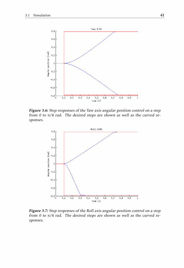
Figure 3.6: Step responses of the Yaw axis angular position control on a stepfrom 0 to π/4 rad. The desired steps are shown as well as the curved re-sponses.
Figure 3.7: Step responses of the Roll axis angular position control on a stepfrom 0 to π/4 rad. The desired steps are shown as well as the curved re-sponses.

42 3 Implementation and control
Figure 3.8: Step responses of the Pitch axis angular position control on astep from 0 to π/4 rad. The desired steps are shown as well as the curvedresponses.
3.1.3 Gyro stabilization
A cosine wave on each axis, representing a angular velocity in zero frame, was fedinto the imusim block described in 3.1.2. In order to counter this distortion thecontrol system had to subtract the, by the gyro, measured angular velocity andposition from the reference signals and then transform them to controller inputs.Figures 3.9 to 3.12 show the results for gyro stabilization around the angularpositions Ω = (0, 0, 0).

3.1 Simulation 43
Figure 3.9: Simulated gyro stabilization of a positional distortion in Pitch inzero frame as a sine wave with a frequency of 5 Hz and an amplitude of 10degrees. The thin curve is the distortion in zero frame and the bold is theangular position integrated from the IMU signal.
Figure 3.10: Simulated gyro stabilization of a positional distortion in Roll inzero frame as a sine wave with a frequency of 2 Hz and an amplitude of 10degrees. The thin curve is the distortion in zero frame and the bold is theangular position integrated from the IMU signal.

44 3 Implementation and control
Figure 3.11: Simulated gyro stabilization of a positional distortion in Yaw inzero frame as a sine wave with a frequency of 1.215 Hz and an amplitude of10 degrees. The thin curve is the distortion in zero frame and the bold is theangular position integrated from the IMU signal.
Figure 3.12: Simulated gyro stabilization of a positional distortion in Rollin zero frame as a sine wave with a frequency of 2 Hz and an amplitudeof 10 degrees. Thin curve is the desired joint angular velocity to the to thecontroller and bold curve is the output angular velocity in the roll joint.

3.1 Simulation 45
Figures 3.9 to 3.11 show distortion in frequencies when the gyro stabilization isstill "acceptable". The ability of gyro stabilization depends on the angular velocitycapability of the joints. The pitch axis has a good stabilization due to its highspeed whereas the other two axes have much lower stabilization ability at higherfrequencies. This is particularly evident in the unbalanced roll axis (Figure 3.10)where the speed capability is greater when the desired angular velocity is in thenegative direction, see Figure 3.12 and Figure 3.4. These simulations show thatthe motors are much too weak to obtain a good gimbal performance.
Influence by increased noise
The noise measured in section 2.4.2 is relatively small and does not have muchimpact on the gyro stabilization simulations. If the variances of the noise in theIMU’s gyros are multiplied by a factor of 1e6 the results are as shown in Figure3.13. The drift in the angular position is because the control system is entirely re-lying on the accuracy of the IMU gyro measurements and has no other reference.Increased noise in the joint encoders does not have any significant impact on thegyro stabilization. This is because the control system only uses the control errorfrom the IMU. This would not be the case if the IMU gyros and the encoders wereread at different sample rates or if the joints are controlled directly, for instanceduring initiations and calibrations.
Figure 3.13: Gyro stabilization test on pitch where the variance of the mea-surement noise in the IMU gyros was multiplied by a factor of 1e6 (all axes).The thin curve is the angular position, as integrated from the IMU signals,and the bold curve is the angular position, as measured without any noise.

46 3 Implementation and control
3.2 Hardware Implementation
The control implementation on the gimbal controller card is written in C-codeand uses the same kinematic functions (section 2.2.2) as the control structurein the simulation environment. The major challenge in hardware programmingwas to implement the encoders and the gyros and accelerometers on the IMUcorrectly and use their data to derive the different angles and angular velocitiesneeded. The controllers were then tuned with the simulation results in section3.1.2 as a starting reference.
3.2.1 Numerical representation
To eliminate the need for floating-point calculations, floating-point numbers arerepresented as Texas Instruments (TI) IQ24 numbers:
IQ24(number) = number × 224. (3.5)
The IQ number can be treated as any integer or used by TI-special functions suchas correct multiplications and trigonometric functions. The scale 224 is a tradeoffbetween numerical accuracy and the range of possible values, in this case range±128 and accuracy 6 · 10−8. The scaling factor can vary between 21 and 230 wherea larger scaling factor means higher accuracy but a smaller range.
3.2.2 Code structure
Figure 3.14 shows a block diagram over the control structure in the hardwareimplementation. It can be compared to Figure A.1. A flow chart of the programcode is shown in Figure 3.15. The program contains the following parts:
Input reading
The gimbal controller has the ability to read input data from a computer via se-rial communication (USB converted to UART). The input data consists of stringswhich are interpreted by the controller. The data is usually a new desired angleαd or angular velocity Φd in the camera space but it has also been used for settingdesired joint positions Θd or joint angular velocities Ωd and new PID controllerparameters.
Update of joint states
The rotary encoder on gimbal axis i measures its current angular position andsends it as a 10 bit binary number to the control unit. The control unit scales thenumber to an angle θi in radians (in IQ24 presentation, section 3.2.1). θi , whichoriginally lies in the range 0...2π, is also converted to lie in the range −π...π. Thismeans θi = 0 on the gimbal is 180 degrees from angle 0 on the encoder.
3.2 Hardware Implementation 47
If the angular distance between two measurements at sample k and k − 1 is largeenough it is used to approximate the angular velocity ωi using the sample fre-quency Fs = 100 Hz.
ωi(k) = (θi(k) − θi(k − 1)) Fs (3.6)
The angles θi and the angular velocities ωi are filtered using a simple exponentialmoving average:
θi =12θi +
12θi,raw (3.7)
and
ωi =34ωi +
14ωi,raw, (3.8)
where θi,raw and ωi,raw are the unfiltered angular position and velocity in thecurrent sample. The smoothing factors a = 1
2 and a = 14 were only roughly tuned
until an acceptable balance between accuracy and smoothness was believed to befound.
Update of IMU states
The gyros on the IMU close to the camera mounting point measures the current
yaw, roll and pitch angular velocities Φ =[φyaw, φroll , φpitch
]Tof body 3 around
its own axes. It is set to measure in the range of 0... ± 2000 /s and sends themeasured angular velocities to the control unit as 15 bit binary numbers whichare then scaled to radians in the IQ24 representation (section 3.2.1). The mea-surements are calibrated by subtracting a bias measured at the beginning of eachgimbal session.
Φ is used to calculate the current angular position relative to the ground α. Asmentioned in section 2.1.2 attitude calculations using the measured angular ve-locities suffer from angular drift due to accumulated measurement errors. A sim-ple approximate integration of Φ using the sample frequency Fs in this case alsocaused problem with angular drift. This was however solved by the use of a com-plementary filter already written by IA. The details of this filter were not studiedenough to be presented in this thesis but basic function is to integrate the by gyromeasured angular velocity to an attitude which is filtered using the translationalacceleration Γ . This acceleration is measured by accelerometers on the IMU andare sent to the control unit in a similar way as the angular velocities.
Inverse kinematics
The desired camera angular position αd or the desired camera angular velocityΦd is transformed to reference signals to the joint controllers in the same way asin section 3.1.2 using equations in section 2.2.2 and equation (3.4).

48 3 Implementation and control
Update of control signals
The code for the PID-controllers was written in according to Algorithm 3.1. Theaccumulated integral term I , the additional term a and the proportional part pare stored in a static structure to be used in the next sample. In total there are 6structures, one for each joint state.
As in the simulation environment in section 3.1.2 the angular position controllertakes the desired angular positions from the inverse kinematics as reference sig-nals and outputs the desired angular velocity for each axis. These angular veloc-ities are added to the desired angular velocities Ωd from the inverse kinematicswhich become reference signals to the angular velocity controller. The outputfrom the angular velocity controller is a number between 0 and ±1 in the IQ24representation. This number is rescaled to an integer between 0 and ±1000 whichis the permille (‰) of the PWM signal to the motor output ports, or the permilleof the maximum voltage to the motors. The voltages create a torque on eachmotor according to section 2.3.2, which sets the gimbal in motion.
Figure 3.14: Block diagram of the control structure in the gimbal hardwareimplementation.

3.2 Hardware Implementation 49
Figure 3.15: Flow chart of one loop in the gimbal control code after initiationand calibration.
3.2.3 Control tuning
The PID-controllers of the gimbal were tuned by first applying the PID parame-ters which were tuned in the simulations described in section 3.1.2. These werethen adjusted to attain acceptable performance in the real application.
Angular velocity
The PID-parameters from the simulations (section 3.1.2) yielded unstable resultswhen used in the real gimbal control. The approach to tune the controller pa-rameters on each axis was to keep the proportional gains K from the simulationsand adjust the integral time Ti until performance was deemed acceptable. Thisresulted in the responses in Figures 3.16 to 3.18 and the parameters in table 3.1.Two of the gain parameters K were also slightly adjusted. The results of theangular velocity control became somewhat oscillative but still but were still con-sidered acceptable with a balance between rise time, oscillations and accuracy.Worth mentioning is the difference in behaviour between the first and secondtransients in Figure 3.16 where the angular velocity in yaw axis steps back 0rad/s are much more oscillative than the first steps. A possible explanation is thenonlinear behaviour in the Yaw axis. The gimbal turns to around 180 degreesduring both motions and stops in the same angular position where the behaviourof the joint is different from the behaviour when the yaw axis is in angular posi-tion 0 degrees. Another set of controller parameters would be more appropriatein this angular position. It is also worth to notice that the pitch signal in Figure3.18 is much noisier when the gimbal is given a angular velocity than when the

50 3 Implementation and control
angular velocity is zero. A possible explanation is that the motion itself inducessmall vibrations in the joint and in the body.
Table 3.1: Angular velocity PI parameters in the real gimbal control, param-eters from simulations in parentheses.
Axis (direction) K TiYaw (+) 1.5(1.5) 0.05(0.007)Yaw (-) 1.5(1.8) 0.05(0.008)Roll (+) 0.8(0.8) 0.05(0.02)Roll (-) 0.4(0.5) 0.05(0.02)Pitch (+) 0.08(0.08) 0.01(0.005)Pitch (-) 0.07(0.07) 0.01(0.005)
The relatively large difference between the Ti parameters from the real controland from the simulations can be explained by looking at the angular velocityrise times in the figures with the adjusted friction parameters in section (2.4.1).The rise time of the simulation in Figure 2.5 is for instance relatively close tozero whereas the actual rise time is longer. In tuning methods, such as Ziegler-Nichols or Åström-Hägglund [Glad and Ljung, 2006, p. 56] where step responsesare used to get reasonable values of the control parameters, the integral time Tiis proportional to the rise time which means that a longer rise time demands alonger integral time. If Ti is too small, it will create a too large integral term inthe control (see Algorithm 3.1).

3.2 Hardware Implementation 51
(a) Positive step.
(b) Negative step.
Figure 3.16: Step responses of the angular velocity in the yaw axis withtuned PID parmeters. Figure a) shows a step from 0 to π/4 rad and b) astep from 0 to −π/4 rad.

52 3 Implementation and control
(a) Positive step.
(b) Negative step.
Figure 3.17: Step responses of the angular velocity in the roll axis with tunedPID parmeters. Figure a) shows a step from 0 to π/4 rad and b) a step from0 to −π/4 rad.

3.2 Hardware Implementation 53
(a) Positive step.
(b) Negative step.
Figure 3.18: Step responses of the angular velocity in the pitch axis withtuned PID parmeters. Figure a) shows a step from 0 to π/4 rad and b) a stepfrom 0 to −π/4 rad.

54 3 Implementation and control
Angular position
The gains K for the angular positions of the gimbals axes were adjusted from 50to 40 in order to obtain smoother results. Figures 3.19 to 3.21 show the desiredangular position and with IMU estimated angular position of the camera. Figure3.21b also shows the desired and measured angular position in the pitch joint toillustrate the nature of the angular position estimates. The overshoots in Figure3.21b occur because the complementary filter mentioned in 3.2.2. The filter usesboth integration of the angular velocities from the gyros and the direction of thetranslational acceleration from the accelerometers. The angular velocity part isvery sensitive to changes but the acceleration part reacts much slower so it takesa while before the estimates are adjusted. The positional control follows thisadjustment.
Figure 3.19: Step response of the angular position in the yaw axis with tunedPID parmeters. Step from 0 to π/4 rad.
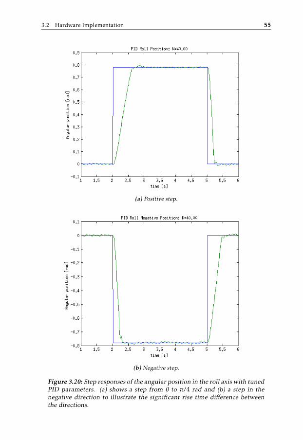
3.2 Hardware Implementation 55
(a) Positive step.
(b) Negative step.
Figure 3.20: Step responses of the angular position in the roll axis with tunedPID parameters. (a) shows a step from 0 to π/4 rad and (b) a step in thenegative direction to illustrate the significant rise time difference betweenthe directions.

56 3 Implementation and control
(a) IMU space
(b) Joint space.
Figure 3.21: Step responses of the angular position in the pitch axis withtuned PID parameters. (a) shows the angular position estimated in the com-plementary filter (Section 3.2.2). (b) Shows the angular position in jointspace (bold curve) and the desired joint angular position (solid, thin curve).The dashed curve is the angular position in IMU space, same as in (a).

3.2 Hardware Implementation 57
3.2.4 Gyro stabilization
Tests were done to determine the gimbal controller’s ability to perform activestabilization of the camera. This was done by comparing a measured motion inbody frame (0) to the motion in body frame (3) (see Figures 2.1 and 2.2). Themeasurements in frame (3) were done with the IMU connected to the gimbalcontrol unit and the measurements in frame (0) were done with a second IMUconnected to a separate control unit. The two control units were not synchronizedso the same disturbance motion was recorded at different times by the two units.This time difference was about 1.5 seconds. There was also an angular drift inthe yaw axis of the IMU on body (0) but, as testing was mainly concerned withthe local amplitudes and frequencies and not the angular position, this did notcause a problem.
Figures 3.22 to 3.24 show the results from tests where the entire gimbal was givena motion in one axis at a time. The gimbal was held by hand in body (0) and wasturned in the yaw axis or rocked in the roll and pitch axis of that body. Figure3.25 shows the results when the gimbal was moved in all three axes. All thesemeasurement started in the IMU angular position α = (0, 0, 0)T .

58 3 Implementation and control
(a) Motion measured in body (0).
(b) Motion measured in body (3).
Figure 3.22: The result from a test of the gyro stabilization in the yaw axis.(a) shows the measurement of the motion of the entire gimbal measured witha IMU attached to body (0) (Figure 2.1). (b) shows the motion of body (3)measured with the IMU there. The measurements were not synchronized,the upper measurement started about 1.5 s before the lower.
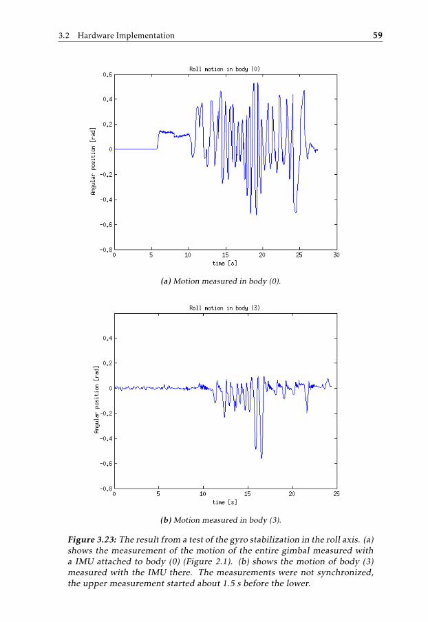
3.2 Hardware Implementation 59
(a) Motion measured in body (0).
(b) Motion measured in body (3).
Figure 3.23: The result from a test of the gyro stabilization in the roll axis. (a)shows the measurement of the motion of the entire gimbal measured witha IMU attached to body (0) (Figure 2.1). (b) shows the motion of body (3)measured with the IMU there. The measurements were not synchronized,the upper measurement started about 1.5 s before the lower.

60 3 Implementation and control
(a) Motion measured in body (0).
(b) Motion measured in body (3).
Figure 3.24: The result from a test of the gyro stabilization in the pitch axis.(a) shows the measurement of the motion of the entire gimbal measured witha IMU attached to body (0) (Figure 2.1). (b) shows the motion of body (3)measured with the IMU there. The measurements were not synchronized,the upper measurement started about 1.5 s before the lower.

3.2 Hardware Implementation 61
(a) Yaw measured in body (0). (b) Yaw measured in body (3).
(c) Roll measured in body (0). (d) Roll measured in body (3).
(e) Pitch measured in body (0). (f) Pitch measured in body (3).
Figure 3.25: The results from a test of the gyro stabilization in all three axeswhere the gimbal was rocked in all three directions. The figures to the leftshow the measurements of the motion of the entire gimbal measured witha IMU attached to body (0) (Figure 2.1). The figures to the right show themotion of body (3) measured with the IMU there. The measurements werenot synchronized, the measurements to the left started about 1.5 s before theones to the right.

62 3 Implementation and control
The results are similar to the results from the simulations in section 3.1.3. Theability to stabilize differs between the axes. The pitch axis has a very good stabi-lization while the ability in the roll and yaw axis is poorer when the frequencyis increased to somewhere around 1 to 2 Hz. This, again illustrates the need formuch stronger actuators to obtain the needed angular velocities.

4Conclusions and discussion
This final chapter contains some conclusions drawn in this thesis, thoughts onwhat could have been done differently, and suggestions for future work.
4.1 About the modelling
The model of the gimbal derived in chapter 2 in this thesis does not exactly matchthe behaviour of the real gimbal but is, for instance, sufficient for developmentof control structures. One of the hardest parts of this work was to verify that thetransformations between the different coordinate frames were correct. This wasdone by moving the joints of a crude little physical model of the gimbal and per-forming the same motions in the simulation environment. It was important thatthis was done before the hardware implementation in order to avoid damages tothe gimbal due to unexpected motions.
The method using Lagrange equations with link transformation matrices in sec-tion 2.3.1 provides a way to calculate the dynamic model using fairly simple pro-gramming in Matlab. However the calculation did take a lot of time, especiallyif simplification algorithms were used in the process. The expressions did alsobecame very cumbersome. They was improved slightly by transferring them toMathematica and using the simplification algorithms included in the program.The results would probably be even better, in terms of faster computations andmore compact expressions, if all calculations had been done using Mathematicaor other tools for symbolic calculations.
63

64 4 Conclusions and discussion
4.1.1 What could had been done differently
As mentioned in the end of section 2.3.2 the actuators could be treated as separatebodies in the model, this to to allow testing of different motors and gearboxeswithout the need to calculate an entirely new model. This would also have beenuseful to find more powerful actuators and also test how the performance wasaffected by their increased size and mass..
Parameters of the gimbal were taken from drawings in CAD software. The samekind of software could be used to simulate a multi body systems and even de-velop control systems around them. However, this possibility was not studied inthis thesis. One argument for the mathematical modelling method used in thisthesis is that it is, in principle independent of expensive software (even tough thedimensions and masses could be less accurate if measured by hand and the calcu-lations would be tedious without proper linear algebra software). The accuracy ofthe model would probably increase with more powerful tools for identificationof unknown parameters, mentioned in section 2.4. Simulations could also bedone in any programming language, provided differential equation solvers wereavailable.
4.1.2 Suggested future work
As explained in section 2.4.1 model accuracy can be improved by more sophisti-cated identification methods. This would create a model accurate enough to beused in model based control methods or as residuals in diagnostics systems. Im-plementing the model in hardware would probably require a more powerful pro-cessor and better simplification algorithms to get less complicated expressions.
Modelling methods where powerful mechanics software is used should also beevaluated.
4.2 About the control structure
The control system of the gimbal was only developed to perform around onepoint (α = (0, 0, 0)) and did not get more advanced controllers than a P-controllerfor angular position and a PI-controller for angular velocity of each axis. Onebig advantage of PI(D)-controllers is that they are relatively simple to work withfor someone with limited prior knowledge of control theory. The hardest part ofthe control design, apart from the work of writing the code, was to derive andverify the transformations between camera and joint frames. This needed to bedone with great care to avoid unexpected motions that could potentially damagethe gimbal. The implementation was successful and no unexpected motions wereobserved.

4.2 About the control structure 65
4.2.1 What could have been done differently
The sample rate in the control system was set quite low (100 Hz). Higher samplerates would probably give some performance improvement. The low sample ratewas mainly to avoid data loss in the serial communication between the gimbaland a computer.
4.2.2 Suggested future work
The performance would probably be improved if linearization was used. It wassuggested during the thesis to have different sets of control parameters for differ-ent configurations of the gimbal, however, this was not implemented. Changes inthe mass moments of inertia resulting from camera reorientation would lead tovarying performance at different angular positions of the camera. Linearizationwould be done by having a number of angles as linearization points and havinga catalogue of control parameters which become active in the vicinity of theirassigned linearization points. Interpolation between the points has also been dis-cussed.
Other types of controllers, such as lead-lag or LQ-controllers, should be evalu-ated. With better performance of the actuators and therefore higher accelerations,coupling effects between the joint states would become a bigger problem. The re-sults from Seong et al. [2006] suggests that a LQG/LTR control (Linear QuadraticGaussian control with Loop Transfer Recovery) would perform better in terms ofdecoupling.
With more powerful microprocessors it would be interesting to use model basedcontrol, as suggested in 4.1.2. One other possibility would also be to send a modelbased feed-forward signal to the platform with information about the gimbalmotion so the platform control could counteract platform motion due to motionof the gimbal. This would reduce the risk of unstable oscillations induced bythe control systems. The model would be a Newton-Euler dynamic model of thereaction forces in the yaw joint.

ASimulink control structure
Figure A.1 shows the control structure in the Simulink environment. In broadstrokes, it can be interpreted in the following way: The blocks in the upper partof the structure pertain to states in joint coordinate space; control of joint angularposition and velocity in interaction with the mathematical model of the gimbal.The "invpos" and "invel" blocks in the middle of the structure are the transfor-mations between IMU coordinate space and joint space. The blocks in the lowerright corner model the behaviour of the gyros (and the magnetometer) in theIMU and external manipulation of the gimbal. More detailed descriptions of thecontrol structure can be found in section 3.1.2.
67

68 A Simulink control structure
Figure A.1: Control structure in Simulink.
Bibliography
T Glad and L Ljung. Reglerteknik: grundläggande teori. Studentlitteratur, 2006.Cited on pages 39 and 50.
Industriell reglerteknik. Kurskompendium. Reglerteknik, Institutionen för sys-temteknik, Linköpings Universitet, 581 83 Linköping, 2009. Cited on page37.
R N Jazar. Theory of Applied Robotics: Kinematics, Dynamics, and Control.Springer, 2007. Cited on pages 11, 12, 15, 18, 19, 20, 21, and 23.
Y S Kwon, H Y Hwang, and Y S Choi. Stabilization loop design on direct drivegimbaled platform with low stiffness and heavy inertia. In International Con-ference on Control, Automation and Systems, 2007. Cited on pages 4 and 5.
N Mohan, T M Undeland, and W P Robbins. Power Electronics, Converters, Ap-plications, and design. Wiley, 2003. Cited on page 24.
T Parveen. Dynamic analysis of 8-joint gimbal system executing 4 dof motion.In International Bhurban Conference on Applied Sciences & Technology, 2009.Cited on page 4.
K J Seong, H G Kang, B Y Yeo, and H P Lee. The stabilization loop design for a two-axis gimbal system using LQG/LTR controller. In SICE-ICASE InternationalJoint Conference, 2006. Cited on pages 5 and 65.
K J Seong, H G Kang, B Y Yeo, and H P Lee. The digital anti-windup LQG/LTRcontroller design for a two axis gimbal system. In International Conference onControl, Automation and Systems, 2007. Cited on page 5.
Y B Shtessel. Sliding mode stabilization of three axis inertial platform. In SystemTheory, 1994., Proceedings of the 26th Southeastern Symposium, 1999. Citedon page 5.
P Skoglar. Modelling and control of IR/EO-gimbal for UAV surveillance appli-cations. master’s thesis lith-isy-ex-3258-2002. Master’s thesis, Department ofElectrical Engineering, Linköpings Universitet, 2002. Cited on page 4.
69

70 Bibliography
B J Smith, W J Schrenk, W B Gass, and Y B Shtessel. Sliding mode control ina two axis gimbal system. In Aerospace Conference, 1999. Proceedings. 1999IEEE, 1999. Cited on page 5.

Upphovsrätt
Detta dokument hålls tillgängligt på Internet — eller dess framtida ersättare —under 25 år från publiceringsdatum under förutsättning att inga extraordinäraomständigheter uppstår.
Tillgång till dokumentet innebär tillstånd för var och en att läsa, ladda ner,skriva ut enstaka kopior för enskilt bruk och att använda det oförändrat för icke-kommersiell forskning och för undervisning. Överföring av upphovsrätten viden senare tidpunkt kan inte upphäva detta tillstånd. All annan användning avdokumentet kräver upphovsmannens medgivande. För att garantera äktheten,säkerheten och tillgängligheten finns det lösningar av teknisk och administrativart.
Upphovsmannens ideella rätt innefattar rätt att bli nämnd som upphovsmani den omfattning som god sed kräver vid användning av dokumentet på ovanbeskrivna sätt samt skydd mot att dokumentet ändras eller presenteras i sådanform eller i sådant sammanhang som är kränkande för upphovsmannens litteräraeller konstnärliga anseende eller egenart.
För ytterligare information om Linköping University Electronic Press se förla-gets hemsida http://www.ep.liu.se/
Copyright
The publishers will keep this document online on the Internet — or its possi-ble replacement — for a period of 25 years from the date of publication barringexceptional circumstances.
The online availability of the document implies a permanent permission foranyone to read, to download, to print out single copies for his/her own use andto use it unchanged for any non-commercial research and educational purpose.Subsequent transfers of copyright cannot revoke this permission. All other usesof the document are conditional on the consent of the copyright owner. Thepublisher has taken technical and administrative measures to assure authenticity,security and accessibility.
According to intellectual property law the author has the right to be men-tioned when his/her work is accessed as described above and to be protectedagainst infringement.
For additional information about the Linköping University Electronic Pressand its procedures for publication and for assurance of document integrity, pleaserefer to its www home page: http://www.ep.liu.se/
© Jakob Johansson