A R C H I V E S O F M E T A L L U R G Y A N D M A T E R I A L S

Volume 58 2013 Issue 1

DOI: 10.2478/v10172-012-0159-4

B. HADAŁA∗, Z. MALINOWSKI∗, T. TELEJKO∗, A. CEBO-RUDNICKA∗, A. SZAJDING∗

INFLUENCE OF THE FINITE ELEMENT MODEL ON THE INVERSE DETERMINATION OF THE HEAT TRANSFERCOEFFICIENT DISTRIBUTION OVER THE HOT PLATE COOLED BY THE LAMINAR WATER JETS

WPŁYW MODELU METODY ELEMENTÓW SKOŃCZONYCH NA WSPÓŁCZYNNIKA WYMIANY CIEPŁAWYZNACZANY Z ROZWIĄZANIA ODWROTNEGO PROCESU LAMINARNEGO CHŁODZENIA PŁYTY METALOWEJ

The industrial hot rolling mills are equipped with systems for controlled cooling of hot steel products. In the case ofstrip rolling mills the main cooling system is situated at run-out table to ensure the required strip temperature before coiling.One of the most important system is laminar jets cooling. In this system water is falling down on the upper strip surface.The proper cooling rate affects the final mechanical properties of steel which strongly dependent on microstructure evolutionprocesses. Numerical simulations can be used to determine the water flux which should be applied in order to control striptemperature. The heat transfer boundary condition in case of laminar jets cooling is defined by the heat transfer coefficient,cooling water temperature and strip surface temperature. Due to the complex nature of the cooling process the existing heattransfer models are not accurate enough. The heat transfer coefficient cannot be measured directly and the boundary inverseheat conduction problem should be formulated in order to determine the heat transfer coefficient as a function of coolingparameters and strip surface temperature. In inverse algorithm various heat conduction models and boundary condition modelscan be implemented. In the present study two three dimensional finite element models based on linear and non-linear shapefunctions have been tested in the inverse algorithm. Further, two heat transfer boundary condition models have been employedin order to determine the heat transfer coefficient distribution at the hot plate cooled by laminar jets. In the first model heattransfer coefficient distribution over the cooled surface has been approximated by the witch of Agnesi type function with theexpansion in time of the approximation parameters. In the second model heat transfer coefficient distribution over the cooledplate surface has been approximated by the surface elements serendipity family with parabolic shape functions. The heat transfercoefficient values at surface element nodes have been expanded in time by the cubic-spline functions. The numerical tests haveshown that in the case of heat conduction model based on linear shape functions inverse solution differs significantly fromthe searched boundary condition. The dedicated finite element heat conduction model based on non-linear shape functions hasbeen developed to ensure inverse determination of heat transfer coefficient distribution over the cooled surface in the time ofcooling. The heat transfer coefficient model based on surface elements serendipity family is not limited to a particular formof the heat flux distribution. The solution has been achieved for measured temperatures of the steel plate cooled by 9 laminarjets.

Keywords: head transfer coefficient, finite element model, inverse solution

Nowoczesne linie walcowania blach na gorąco posiadają instalacje do wymuszonego chłodzenia. Jego celem jest kontro-lowanie szybkości zmian temperatury blachy w całej objętości zapewniając tym wymaganą strukturę i własności mechaniczne.Chłodzenie jest prowadzone w końcowej części linii technologicznej, w której nad górną i pod dolną powierzchnią gorącegopasma umieszczone są urządzenia dostarczające wodę chłodzącą. Z uwagi na sposób podawania wody chłodzącej można jepodzielić na trzy główne systemy: chłodzenie laminarne, chłodzenie z użyciem kurtyn wodnych oraz chłodzenie natryskiemwodnym. W istniejących liniach walcowniczych można spotkać kombinacje poszczególnych systemów. Projektowanie systemówchłodniczych jest trudne i musi być wspomagane przez modele matematyczne i numeryczne wymiany ciepła między gorącąpowierzchnią blachy a wodą i otoczeniem. Podstawowe znaczenie dla symulacji procesu ma przyjęcie poprawnych wartościwspółczynników wymiany ciepła, których znajomość w dużej mierze determinuje dokładność obliczeń. Współczynnik wymianyciepła nie może być zmierzony bezpośrednio i konieczne jest zastosowanie rozwiązańodwrotnych zagadnienia przewodzeniaciepła. W algorytmach odwrotnych możliwe jest użycie różnych modeli do rozwiązania równania przewodzenia ciepła. Za-stosowane modele w istotnym stopniu wpływają na jakość rozwiązania odwrotnego. W pracy przedstawiono wyniki testówdwóch modeli przewodzenia ciepła opartych na liniowych i nieliniowych funkcjach kształtu w algorytmie metody elementówskończonych. Testowano również dwa modele aproksymacji warunku brzegowego. Wybrany model warunku brzegowego i mo-del metody elementów skończonych wykorzystujący nieliniowe funkcje kształtu zastosowano do wyznaczenia współczynnikawymiany ciepła w procesie chłodzenia gorącej płyty stalowej 9 strumieniami wody swobodnie opadającej na jej powierzchnię.

∗ AGH UNIVERSITY OF SCIENCE AND TECHNOLOGY, DEPARTMENT OF HEAT ENGINEERING AND ENVIRONMENT PROTECTION, 30-059 KRAKÓW, AL. MICKIEWICZA 30, POLAND

106

Uzyskano rozwiązanie przedstawiające rozkład współczynnika wymiany ciepła i gęstości strumienia ciepła na powierzchnipłyty w czasie jej chodzenia.

1. Introduction

During the hot rolling operations the strip losses heatmainly by radiation and convection to surrounding air andcooling water. In the roll gap the strip also losses heat tothe rolls, but the time of contact is very short (milliseconds)and the total heat losses are relatively small. However, thestrip surface temperature drop can be high to about 600◦C.More dramatic changes of the strip surface temperature areobserved during descaling with high pressure water jets wherethe strip surface temperature falls to about 100◦C. At the endof hot rolling line the strip temperature is in the range of800-1000◦C and the strip must be cooled down to the re-quired coiling temperature [1]. During water cooling the stripundergoes rapid changes of temperature which have signifi-cant effect on material structure and properties. Thus, the striptemperature control in the hot rolling operations is very im-portant and involves computer modeling. The most importantis a proper determination of heat transfer boundary conditionsduring water cooling at run-out table before coiling. Thereare several methods of cooling one of them are laminar flowcylindrical water jets or water curtains placed above the strip.Hatta et al. [2, 3] have developed empirical equations for heattransfer coefficient (HTC) while cooling 18Cr-8Ni steel plate10 mm thick with water curtain. Two equations have beenproposed, one for nucleate and transition boiling when wateris in direct contact with the plate surface (wetting zone). Thesecond equations have been proposed for film boiling. The heattransfer coefficient for wetting zone has been approximated bythe local Nusselt number for laminar flow of water over theplate surface. The heat transfer boundary condition model hasbeen verified based on the plate temperature measurementsby 3 thermocouples attached to the bottom plate surface (notcooled by water). The assumption of the laminar flow of wa-ter and model validation by temperature measurements 10 mmbelow the water cooled surface are the primary drawbacks inthe heat transfer model. The inverse solution for heat trans-fer coefficient determination while cooling AISI 304L steelby one axially symmetrical water jet have been presented byWang et al. [4]. The plate thickens was 25 mm and the platetemperature was measured by 4 thermocouples located 2.5mm below the cooled surface. The solution has been obtainedon the basis of axially symmetrical heat conduction model.Similar inverse solution for one spray nozzle was proposed byMalinowski at al. [5]. Inverse solutions based on axially sym-metrical models are limited to one spray or jet nozzle only.Inverse solution based on three dimensional heat conductionmodel are required for heat transfer coefficient determinationfor plate cooling by a set of water jets, water sprays or watercurtains. This class of solutions have been presented by Kimet al. [6] and Zhou et al. [7] but only for the simulated tem-perature sensor indications. The solutions have been obtainedfor a large number of simulated sensors, at least one sensor isrequired in element or at element node in the plane of simu-lated sensors locations. Such a large number of sensors willchange material structure and its properties in case of phys-ical experiment. In the paper the inverse solution based on

three dimensional heat conduction model for measured platetemperatures has been obtained.

2. Plate cooling model

The temperature field in the plate cooled by laminar waterjets has been determined from the transient heat conductionequation:

∂T∂τ

=λ

ρc

∂2T∂x2

1

+∂2T∂x2

2

+∂2T∂x2

3

+ qv (1)

where: c – specific heat, T – temperature, qv – internal heatsource, x, y, z – rectangular coordinates, τ – time, λ – thermalconductivity, ρ – density.

The solution of equation (1) gives the plate tempera-ture field for the specified boundary conditions at the platesurfaces. At the water cooled upper plate surface convectionboundary condition has been specified:

q (x1 = h, x2, x3, τ) = α (x1 = h, x2, x3, τ) (Ts − Ta) (2)

where: h – plate height, Ts – plate surface temperature, Tp –water temperature.

Heat transfer coefficient α at the water cooled surface hasbeen defined as a function of surface coordinates and the timeof cooling. Two boundary condition models have been testedin the inverse solution to the heat conduction problem (IHCP).

In the first boundary condition model (Model A) for theapproximation of the HTC distribution over the cooled surfacethe witch of Agnesi type function has been chosen:

α(x1 = h, x2, x3, τ) =[αmax(τ)]3

(c (τ) (x2 − b/2))2 + [αmax(τ)]2(3)

where: b determines width of the plate, c(τ) is a time depen-dent parameter and αmax(τ) is the maximum value of the heattransfer coefficient at x2 = b/2. Cubic-spline functions havebeen chosen for the expansion in time of the parameters c(τ)and αmax(τ):

c (τ) =

4∑

i=1

Hi(η)pi (4)

αmax (τ) =

4∑

j=1

H j(η)p j for η ∈ (0, 1) (5)

Accuracy of the HTC distribution in the time of coolingcan be improved dividing the cooling time into periods forwhich τ ∈ (τ1,τ2). In this case the local coordinate η is givenby:

η =τ − τ1

τ2 − τ1(6)

The cubic-spline functions H j have the following form:

H1 = 1 − 3η2 + 2η3

H2 = 3η2 − 2η3

H3 = η − 2η2 + η3

H4 = −η2 + η3

(7)

107

The parameters p j define the values of c and αmax parametersand their derivatives with respect to time at nodes of approx-imation.

The boundary condition model A is limited to the HTCdistributions for which maximum value of HTC takes placeat the water jets line for x2 = b/2. However, HTC stronglydepends on the cooled surface temperature and the model Amight not be able correctly reflect HTC distribution for boil-ing heat transfer. More general model B has been developedfor which the HTC distribution over the cooled surface hasbeen approximated by surface elements with quadratic shapefunctions serendipity family:

α (x1 = h, x2, x3, τ) =

8∑

i=1

NiPi (τ) (8)

where Ni are quadratic shape functions serendipity family:

N1= (1−ξ1) (1−ξ2) (−ξ1−ξ2−1) /4

N2=(1−ξ2

1

)(1−ξ2) /2

N3 = (1 + ξ1) (1 + ξ2) (ξ1 − ξ2 − 1) /4

N4=(1−ξ2

2

)(1+ξ1) /2 (9)

N5= (1+ξ1) (1+ξ2) (ξ1+ξ2−1) /4

N6=(1−ξ2

1

)(1+ξ2) /2

N7= (1−ξ1) (1+ξ2) (−ξ1+ξ2−1) /4

N8=(1−ξ2

2

)(1−ξ1) /2 for ξ1∈ (−1, +1) and ξ2∈ (−1,+1)

where ξ1, ξ2 are natural coordinates of the surface element.In the case of boundary condition model B the cooled surfaceis divided into rectangular elements. For each element equa-tion (8) has been used to approximate the HTC distribution.Functions Pi(τ) describe the heat transfer coefficient variationat nodes of elements in the time of cooling. At each elementnode the functionPi(τ) has the following form:

Pi (τ) =

3∑

j=1

W j(η)pi j (10)

where the parabolic-spline functions W j are given by:

W1 = 1 − 3η + 2η2

W2 = 4η − 4η2

W3 = 2η2 − η for 0 6 η 6 1.(11)

In the case of the boundary condition model B the setof unknown parameters pi j which have to be determined inthe inverse heat conduction model is composed of the heattransfer coefficient values at nodes of approximation.

At the lower plate surface, which is free from water, ra-diation boundary condition has been specified:

q (x1 = 0, x2, x3, τ) = 5, 67 ·10−8T 4

s − T 4k

1εs

+SsSk

(1εk− 1

) (12)

where: Sk – cooling chamber surface, Ss – plate surface,Tk –cooling chamber surface temperature, εs – emissivity of the

plate surface, εk – emissivity of the cooling chamber surface.The heat flux at the lower plate surface which is not cooledby water is very small (about 0.5%) compared to heat flux forwater cooling and natural convection neglected in equation(12) and possible inaccuracy in emissivity determination willnot have any practical influence on the inverse solution to theHTC at the water cooled surface.

In the IHCP solution only part of the plate is consideredas shown in Fig. 1. At the side surfaces of the plate whichcover less than 13% of the total boundary surface zero heatflux boundary conditions have been assumed:

q (x1, x2 = 0, x3, τ) = −λ ∂T∂x2

= 0 (13)

q (x1, x2 = b, x3, τ) = −λ ∂T∂x2

= 0 (14)

q (x1, x2, x3 = 0, τ) = −λ ∂T∂x3

= 0 (15)

q (x1, x2, x3 = l, τ) = −λ ∂T∂x3

= 0 (16)

where: b – width of the plate, l – length of the plate.

Fig. 1. The plate cooling model employed in the inverse solution tothe 3D heat conduction problem

It is expected that the heat gains at the side surfaces ofthe plate neglected in the IHCP will be less than 0.05% of theheat flux for water cooling.

In the heat conduction equation (1) qv represents the in-ternal heat source. In the case of steel plate cooling heat gen-eration due to phase transformation should be included in theIHCP. However, it would require a separate model for heatgeneration dedicated for the inverse solution. In the presentstudy inconel alloy and steel grade which do not involve phasetransformation in the examined temperature range has beenselected to avoid influence of heat generation on the HTCdetermination. In such cases qv =0.

The unknown parameters p j or pi j which define the HTCdistribution in developed boundary conduction models A andB have to be determined by minimizing the objective function:

E (pi) =

Nt∑

m=1

Np∑

n=1

(Tem

n − Tmn

)2 (17)

where: pi is the vector of the unknown parameters composedof parameters p j or pi j, Nt – number of the temperaturesensors, Np – number of the temperature measurements per-formed by one sensor in the time of cooling, Tem

n – the platetemperature measured by the sensor m at the time τn, Tm

n –

108

the plate temperature at the location of the sensor m at thetime τn calculated from the finite element solution to the heatconduction equation (1).

To solve the heat conduction equation (1) finite elementmethod has been used. By employing the weighted residualsmethod to Eq. (1) two finite element models have been devel-oped. In the first model linear shape function has been used.In the second model non linear weighting and shape functionshave been employed. The detailed description of the two finiteelement models has been presented in [8, 9].

3. Inverse solutions to simulated temperature sensorindications

The developed model for the inverse determination ofheat transfer coefficient has been first tested based on simulat-ed temperature sensor indications. The simulations have beenperformed for the inconel alloy with the conductivity and spe-cific heat presented in Fig. 2. The inconel density has beenassumed as 8470 kg/m3. Simulations have been performed forthe plate with the dimensions of h =10 mm, b =100 mmand l =200 mm. It has been assumed that the initial platetemperature is To =700◦C. The simulated temperature sensorsindications have been achieved in direct simulations of theplate cooling. The temperature variations have been simulatedat 12 points located 1 mm below the cooled surface at x1 =9mm. Locations of points in x2 – x3 plane have been presentedin Fig. 3. In the simulated plate cooling the boundary condi-tion at the upper plate surface has been described by Eq. (3)with the parameter αmax = 1000 W/(m2·K) and c = 50000.At the other boundary surfaces heat loses has been neglect-ed. The assumed parameters describe constant in time heattransfer coefficient distribution over the cooled surface withthe thermal symmetry at the plane x2 = b/2. Since there is nochange of the HTC in x3 direction the temperature variation atpoint P1 is the same as at points: P4, P5, P8, P9, P12. At pointP2 temperature varies in time in the same way as at points:P3, P6, P7, P10, P11. Simulated temperature sensor indicationsobtained in the direct solution have been presented in Fig. 4.Two numerical tests S1 and S2 have been performed based onsimulated temperature sensor indications. Finite element mod-els based on linear (Simulation S1) and non linear (SimulationS2) form functions have been tested in the inverse solution tothe heat conduction problem.

Fig. 2. Heat conduction coefficient and specific heat as functions oftemperature for the inconel alloy

Fig. 3. Locations of the simulated temperature sensors in the x2 –x3

plane 1 mm below the cooled surface

Fig. 4. Simulated temperature sensor indications at point P1 and P2

for the modeled boundary condition described by equation (3) withαmax = 1000 W/(m2·K) and c = 50000

• Simulation S1 – linear weighting and shape functions havebeen employed in the finite element solution to the heatconduction equation (1). The plate has been divided into11×10×2 isoperimetric elements as shown in Fig. 5. Thesolution to the heat conduction problem depends on 396degrees of freedom, which are temperatures at elementsnodes.

• Simulation S2 – non linear weighting and shape functionshave been employed in the finite element solution to theheat conduction equation (1). The plate has been dividedinto 2×2×1 prism elements in x1, x2 and x3 direction,respectively. The solution to the heat conduction problemdepends on 144 degrees of freedom composed of tem-peratures and temperature derivatives at prism elementsnodes.

109

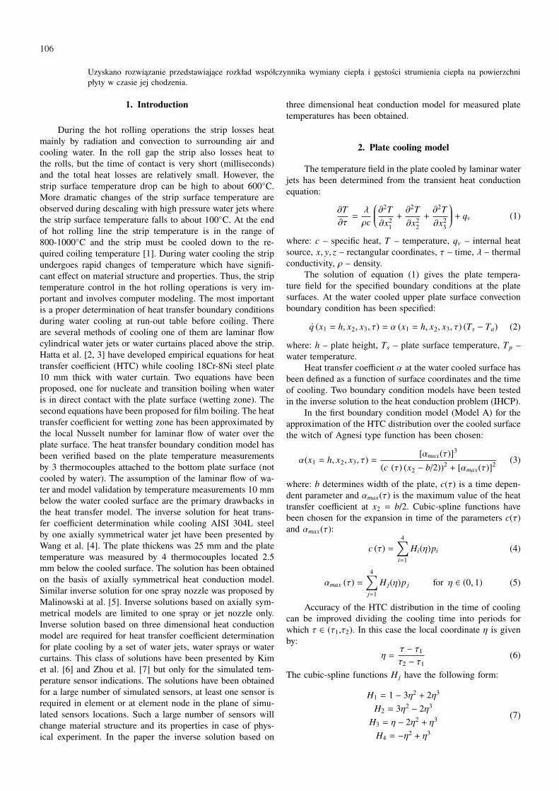
Fig. 5. Division of the cooled plate into linear elements employed inthe simulation S1

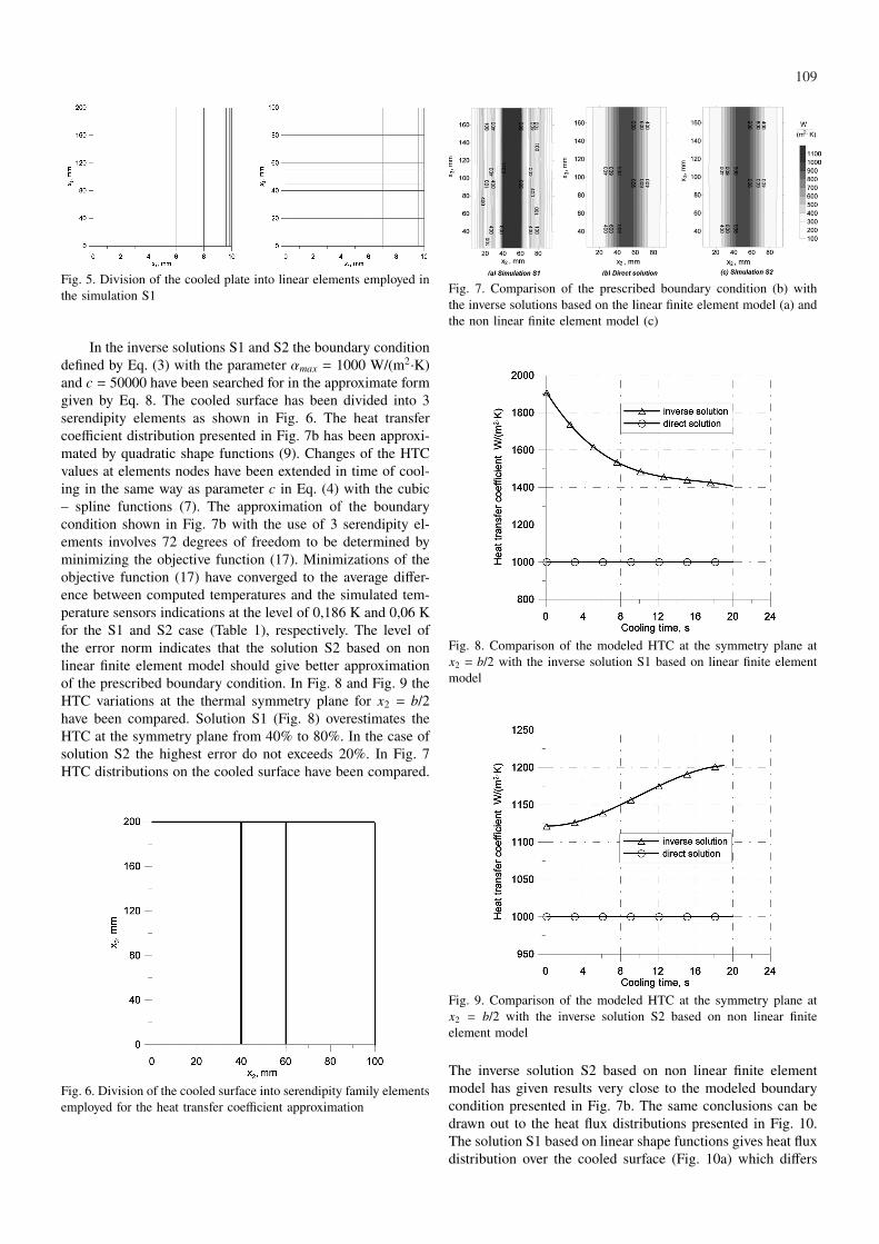
In the inverse solutions S1 and S2 the boundary conditiondefined by Eq. (3) with the parameter αmax = 1000 W/(m2·K)and c = 50000 have been searched for in the approximate formgiven by Eq. 8. The cooled surface has been divided into 3serendipity elements as shown in Fig. 6. The heat transfercoefficient distribution presented in Fig. 7b has been approxi-mated by quadratic shape functions (9). Changes of the HTCvalues at elements nodes have been extended in time of cool-ing in the same way as parameter c in Eq. (4) with the cubic– spline functions (7). The approximation of the boundarycondition shown in Fig. 7b with the use of 3 serendipity el-ements involves 72 degrees of freedom to be determined byminimizing the objective function (17). Minimizations of theobjective function (17) have converged to the average differ-ence between computed temperatures and the simulated tem-perature sensors indications at the level of 0,186 K and 0,06 Kfor the S1 and S2 case (Table 1), respectively. The level ofthe error norm indicates that the solution S2 based on nonlinear finite element model should give better approximationof the prescribed boundary condition. In Fig. 8 and Fig. 9 theHTC variations at the thermal symmetry plane for x2 = b/2have been compared. Solution S1 (Fig. 8) overestimates theHTC at the symmetry plane from 40% to 80%. In the case ofsolution S2 the highest error do not exceeds 20%. In Fig. 7HTC distributions on the cooled surface have been compared.

Fig. 6. Division of the cooled surface into serendipity family elementsemployed for the heat transfer coefficient approximation

Fig. 7. Comparison of the prescribed boundary condition (b) withthe inverse solutions based on the linear finite element model (a) andthe non linear finite element model (c)

Fig. 8. Comparison of the modeled HTC at the symmetry plane atx2 = b/2 with the inverse solution S1 based on linear finite elementmodel

Fig. 9. Comparison of the modeled HTC at the symmetry plane atx2 = b/2 with the inverse solution S2 based on non linear finiteelement model

The inverse solution S2 based on non linear finite elementmodel has given results very close to the modeled boundarycondition presented in Fig. 7b. The same conclusions can bedrawn out to the heat flux distributions presented in Fig. 10.The solution S1 based on linear shape functions gives heat fluxdistribution over the cooled surface (Fig. 10a) which differs

110

essentially from the modeled case shown in Fig. 10b. The platesurface temperature after 20 s of cooling has been shown inFig. 11. The average temperature error presented in Table 1is low for both simulations S1 and S2. However, as it can beseen in Fig. 11 good agreement between modeled temperaturefield (Fig. 11b) and the inverse solution based on linear finiteelement model has been obtained only at locations of simulat-ed measurement points. Inverse solution based on non linearshape functions has given temperature field (Fig. 11c) verysimilar to the modeled case (Fig. 11b). The conducted numer-ical test have shown that the inverse solution based on nonlinear form functions can be employed in determining heattransfer boundary conditions at the cooled plate with goodaccuracy.

Fig. 10. Comparison of the prescribed heat flux (b) with the inversesolutions based on the linear finite element model (a) and the nonlinear finite element model (c)

Fig. 11. Comparison of the cooled surface temperature obtained inthe direct simulation (b) with the inverse solutions based on the linearfinite element model (a) and the non linear finite element model (c)

TABLE 1Average differences between computed temperatures and the

simulated temperature sensors indications

Maximum value of HTC,W/(m2· K) Heat condition model Average error, K

1000S1 0,186

S3 0,06

4. Inverse solution to measured temperatures while waterjets cooling

The developed inverse method based on non linear shapefunctions has been employed to determine the heat transfer

coefficient while cooling steel plate with 9 water jets. Steelplate 210 mm in width, 300 mm in length and 8 mm inheight has been heated in the electric furnace to the uniformtemperature of 811◦C. Hot plate has been pulled from thefurnace and cooled by 9 water jets placed in lines at themiddle of the plate (Fig. 12.). Water jets have been situated0,39 m above the plate. Water flux was 39,04 dm3/(s·m2) andwater temperature was 16,9◦C. The plate temperature havebeen measured by 20 thermocouples located 2 mm below thecooled surface. Thermocouples have been situated in 5 rows.Distance between thermocouples in a row was 20 mm andthe distance between rows was 50 mm. The test sample hasbeen made from H13JS steel. The heat conductivity (Fig. 13),specific heat (Fig. 13) and density (Fig. 14) as functions oftemperature for H13JS steel have been determined from thedata published in [10]. The cooled surface has been dividedinto 4 serendipity elements in x3 direction and 2 elements inx2 direction. Thus, the distribution of the HTC coefficient de-fined by Eq. (8) has been approximated by 8 surface elements.The HTC approximation in time at each node of the surfaceelements has been achieved dividing the time of cooling into 6periods. The model of the HTC approximation over the cooledsurface and in the time of cooling requires 481 pi j parametersin Eq. 10. The parameters have been determined by minimiz-ing the error norm (17). The inverse solution converged tothe average error of 3.01 K between measured and computedtemperatures. In Fig. 15 temperatures measured by one row ofthermocouples situated at the middle of the plate length havebeen compared with the computed temperatures. The com-puted temperatures compare very well to the measured dataover the time of cooling. The inverse solution has given com-plete information about the heat transfer coefficient and heatflux variations over the cooled surface as functions of time. InFig. 16 the HTC distribution over the cooled surface after 20 s

Fig. 12. Schematic for the plate cooling by 9 water jets employed inthe 3D inverse solution to the measured data

Fig. 13. Heat conduction coefficient and specific heat as functions oftemperature for H13JS steel

111

Fig. 14. Density as function of temperature for H13JS steel

Fig. 15. Comparison of the measured and computed temperatures forthe thermocouples located at the middle of the plate length 2 mmbelow the cooled surface

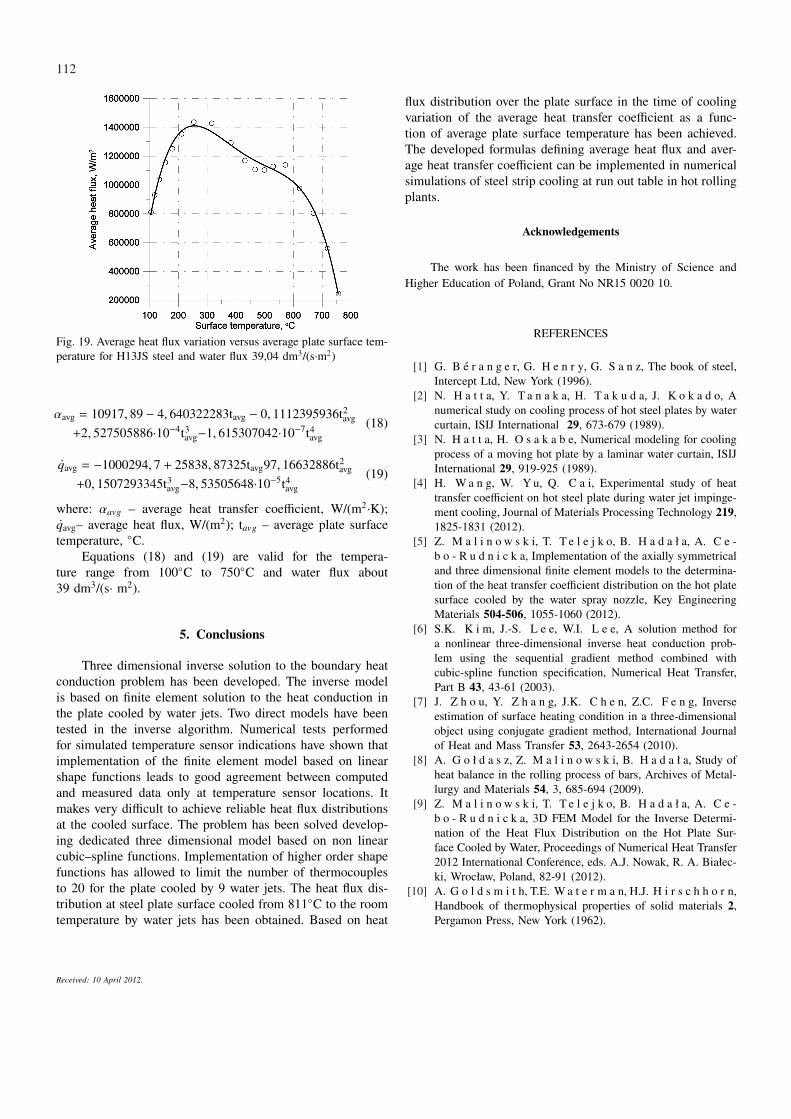
of cooling has been presented. The HTC varies significantlyfrom 100 W/(m2· K) to 12000 W/(m2· K) over the cooledsurface. It affects the cooled surface temperature as it hasbeen shown in Fig. 17. The plate temperature below the waterjets has dropped to about 50◦C but at the distance of 40 mmfrom the water jets the plate temperature at the same time isstill very height and reaches 750◦C. Presented HTC and tem-perature distributions over the cooled surface have shown thatthe plate cooling with the water jets results in significant nonuniformity of the heat transfer boundary conditions. Numericalmodeling of such processes will encounter serious problemswith the boundary condition determination. For practical im-plementations average values can be used. In Fig. 18 averageheat transfer coefficient as function of average surface tem-perature determined based on obtained inverse solution hasbeen presented. The average heat transfer coefficient has beencalculated from the average heat flux (Fig. 19) over the squareof 80×80 mm below the water jets. Presented in Fig. 18 andFig. 19 average heat transfer coefficient and average heat fluxas functions of the average surface temperature can be calcu-lated from the equations:

Fig. 16. Heat transfer coefficient distribution over the plate surfaceafter 20 s of water jets cooling for H13JS steel and water flux 39,04dm3/(s·m2)

Fig. 17. Temperature distribution at the plate surface after 20 s ofwater jets cooling for H13JS steel and water flux 39,04 dm3/(s·m2)

Fig. 18. Average heat transfer coefficient variation versus averageplate surface temperature for H13JS steel and water flux 39,04dm3/(s·m2)

112

Fig. 19. Average heat flux variation versus average plate surface tem-perature for H13JS steel and water flux 39,04 dm3/(s·m2)

αavg = 10917, 89 − 4, 640322283tavg − 0, 1112395936t2avg+2, 527505886·10−4t3avg−1, 615307042·10−7t4avg

(18)

qavg = −1000294, 7 + 25838, 87325tavg97, 16632886t2avg+0, 1507293345t3avg−8, 53505648·10−5t4avg

(19)

where: αavg – average heat transfer coefficient, W/(m2·K);qavg– average heat flux, W/(m2); tavg – average plate surfacetemperature, ◦C.

Equations (18) and (19) are valid for the tempera-ture range from 100◦C to 750◦C and water flux about39 dm3/(s· m2).

5. Conclusions

Three dimensional inverse solution to the boundary heatconduction problem has been developed. The inverse modelis based on finite element solution to the heat conduction inthe plate cooled by water jets. Two direct models have beentested in the inverse algorithm. Numerical tests performedfor simulated temperature sensor indications have shown thatimplementation of the finite element model based on linearshape functions leads to good agreement between computedand measured data only at temperature sensor locations. Itmakes very difficult to achieve reliable heat flux distributionsat the cooled surface. The problem has been solved develop-ing dedicated three dimensional model based on non linearcubic–spline functions. Implementation of higher order shapefunctions has allowed to limit the number of thermocouplesto 20 for the plate cooled by 9 water jets. The heat flux dis-tribution at steel plate surface cooled from 811◦C to the roomtemperature by water jets has been obtained. Based on heat

flux distribution over the plate surface in the time of coolingvariation of the average heat transfer coefficient as a func-tion of average plate surface temperature has been achieved.The developed formulas defining average heat flux and aver-age heat transfer coefficient can be implemented in numericalsimulations of steel strip cooling at run out table in hot rollingplants.

Acknowledgements

The work has been financed by the Ministry of Science andHigher Education of Poland, Grant No NR15 0020 10.

REFERENCES

[1] G. B e r a n g e r, G. H e n r y, G. S a n z, The book of steel,Intercept Ltd, New York (1996).

[2] N. H a t t a, Y. T a n a k a, H. T a k u d a, J. K o k a d o, Anumerical study on cooling process of hot steel plates by watercurtain, ISIJ International 29, 673-679 (1989).

[3] N. H a t t a, H. O s a k a b e, Numerical modeling for coolingprocess of a moving hot plate by a laminar water curtain, ISIJInternational 29, 919-925 (1989).

[4] H. W a n g, W. Y u, Q. C a i, Experimental study of heattransfer coefficient on hot steel plate during water jet impinge-ment cooling, Journal of Materials Processing Technology 219,1825-1831 (2012).

[5] Z. M a l i n o w s k i, T. T e l e j k o, B. H a d a ł a, A. C e -b o - R u d n i c k a, Implementation of the axially symmetricaland three dimensional finite element models to the determina-tion of the heat transfer coefficient distribution on the hot platesurface cooled by the water spray nozzle, Key EngineeringMaterials 504-506, 1055-1060 (2012).

[6] S.K. K i m, J.-S. L e e, W.I. L e e, A solution method fora nonlinear three-dimensional inverse heat conduction prob-lem using the sequential gradient method combined withcubic-spline function specification, Numerical Heat Transfer,Part B 43, 43-61 (2003).

[7] J. Z h o u, Y. Z h a n g, J.K. C h e n, Z.C. F e n g, Inverseestimation of surface heating condition in a three-dimensionalobject using conjugate gradient method, International Journalof Heat and Mass Transfer 53, 2643-2654 (2010).

[8] A. G o ł d a s z, Z. M a l i n o w s k i, B. H a d a ł a, Study ofheat balance in the rolling process of bars, Archives of Metal-lurgy and Materials 54, 3, 685-694 (2009).

[9] Z. M a l i n o w s k i, T. T e l e j k o, B. H a d a ł a, A. C e -b o - R u d n i c k a, 3D FEM Model for the Inverse Determi-nation of the Heat Flux Distribution on the Hot Plate Sur-face Cooled by Water, Proceedings of Numerical Heat Transfer2012 International Conference, eds. A.J. Nowak, R. A. Białec-ki, Wrocław, Poland, 82-91 (2012).

[10] A. G o l d s m i t h, T.E. W a t e r m a n, H.J. H i r s c h h o r n,Handbook of thermophysical properties of solid materials 2,Pergamon Press, New York (1962).

Received: 10 April 2012.