Improving Adversarial Robustness via Guided Complement Entropy

Hao-Yun Chen*1, Jhao-Hong Liang*1, Shih-Chieh Chang1, 2, Jia-Yu Pan3, Yu-Ting Chen3, Wei Wei3,and Da-Cheng Juan3

1Department of Computer Science, National Tsing-Hua University, Hsinchu, Taiwan

2Electronic and Optoelectronic System Research Laboratories, ITRI, Hsinchu, Taiwan3Google Research, Mountain View, CA, USA

{haoyunchen,jayveeliang}@gapp.nthu.edu.twscchang@cs.nthu.edu.tw

{jypan, yutingchen, wewei, dacheng}@google.com

Abstract

Adversarial robustness has emerged as an importanttopic in deep learning as carefully crafted attack sam-ples can significantly disturb the performance of a model.Many recent methods have proposed to improve adversar-ial robustness by utilizing adversarial training or modeldistillation, which adds additional procedures to modeltraining. In this paper, we propose a new trainingparadigm called Guided Complement Entropy (GCE) thatis capable of achieving “adversarial defense for free,” whichinvolves no additional procedures in the process of im-proving adversarial robustness. In addition to maximizingmodel probabilities on the ground-truth class like cross-entropy, we neutralize its probabilities on the incorrectclasses along with a “guided” term to balance betweenthese two terms. We show in the experiments that ourmethod achieves better model robustness with even bet-ter performance compared to the commonly used cross-entropy training objective. We also show that our methodcan be used orthogonal to adversarial training across well-known methods with noticeable robustness gain. To thebest of our knowledge, our approach is the first one thatimproves model robustness without compromising perfor-mance.

1. Introduction

Deep neural networks have been adopted to improvethe performance of state-of-the-arts on a wide varietyof tasks in computer vision, including image classifica-tion [9], segmentation [13], and image generations [6]. Al-beit triumphing on predictive performance, recent liter-

*The authors contribute equally to this paper.

ature [1, 5, 16] has shown that deep neural models arevulnerable to adversarial attacks. In an adversarial at-tack, undetectable but targeted perturbations are addedto input samples which can drastically degrade the per-formance of a model. Such attacks have imposed seriousthreats to the safety and robustness of technologies en-abled by deep neural models. Taking deep learning basedself-driving cars, for example, models might mistakenlyrecognize a “stop sign” as a “green light” when adversarialexamples are present. Needless to say, improving adver-sarial robustness is critical as it saves not only the modelperformance but the lives of people in many cases.

Figure 1. Latent space of the models trained by different objec-tive functions on CIFAR10. Visualization is done using t-SNE.Left: the latent space of model trained with cross-entropy (XE).Right: the latent space of model trained with GCE. Comparedto XE, more distinct clusters (less overlap) are formed for eachclass from the training with GCE.

A wide range of work has been proposed to address theissue of adversarial robustness. One method to improvethe model robustness is “adversarial training” [11, 14, 20]where the model is trained with either adversarial ex-amples [14] or a combination of both natural examples1

1The “natural examples” mentioned in this paper are the normalsamples in the original dataset, which contrasts to the “adversarial ex-amples.”

1

arX

iv:1

903.

0979

9v3

[cs

.LG

] 7

Aug

201

9

and adversarial examples as a form of data augmenta-tion [20]. Here, adversarial examples refer to the arti-ficially samples by adding targeted perturbations to theoriginal data [1, 4, 5, 10, 14, 16]. Other defense methodssuch as Defensive Distillation [17, 18] adopt the conceptof model distillation to teach a smaller version of the orig-inal learned network that is less sensitive to input pertur-bations in order to make the model more robust.

One caveat for using the existing defense mechanism isthat they usually require additional processes, relying oneither adversarial training or an additional teacher modelin the distillation case. The fact that such a procedure isdependent on a specific implementation makes robust-ness improvement less flexible and more computation-ally intensive. The question we ask ourselves in this pa-per is, can we construct a training procedure that is ca-pable of achieving “adversarial defense for free,” meaningthat model robustness is improved in a model-agnosticway without the presence of an attack model or a teachermodel. Another issue with the existing methods is thatadversarial robustness usually come at the cost of modelperformance. A recent analysis [15, 21] has shown thatadversarial training hurts model generalization, and im-provement on robustness is approximately at the samescale as the amount of performance degradation.

In this paper, we propose a novel training paradigmto improve adversarial robustness that achieves adver-sarial defense for free without using additional trainingprocedures. Specifically, we propose a carefully designedtraining objective called “Guided Complement Entropy”(GCE). Different to the usual choice of cross-entropy,which focuses on optimizing the model’s likelihood onthe correct class, we additionally add penalty that sup-presses the model’s probabilities on incorrect classes.Those two terms are balanced through a “guided” termthat scales exponentially. Such a formulation helps towiden the gap in the manifold between ground-truthclasses and incorrect classes, which has been proved to beeffective in recent studies on minimum adversarial dis-tortion [23]. This can be illustrated in Fig 1 where GCEclearly makes the clusters more separable compares tocross-entropy. Training with GCE for model robustnesshas several advantages compares to prior methods: (a) noadditional computational cost is incurred as no adversar-ial example is involved and no extra model is required,and (b) contrary to prior analysis [15, 21] , improvingmodel robustness no longer comes at a cost of model per-formance and we see sometimes better performance assupported in our experiment section.

The contributions of our paper are three-fold. Firstly,to the best of our knowledge, GCE is the first work thatachieves adversarial robustness without compromisingmodel performance. Compares to the widely used meth-

ods which usually incur significant performance drop,our method can maintain or even beat the performance ofmodels trained with cross-entropy. Secondly, our methodis the first approach that is capable of achieving adversar-ial defense for free, which means improving robustnessdoes not incur additional training procedures or com-putational cost, making the method agnostic to attackmechanisms. Finally, our proposed method managed toimprove on top of a wide range of state-of-the-art defensemechanisms. Future work in the field can boost robust-ness improvements across different methods and pushthe frontiers of the adversarial defense forward.

2. Related Work

Adversarial Attacks. Several adversarial attack methodshave been proposed in the “white-box” setting, which as-sumes the structure of the model being attacked is knownin advance. As an iteration-based attack, [5] first in-troduces a fast method to crafting adversarial examplesby perturbing the pixel’s intensity according to the gradi-ent of the loss function. [5] is an example of the single-step adversarial attack. As an extension to [5], [10] it-eratively applies the gradient-based perturbation step bystep, each with a small step size. A further extension to[10] is [4] which adds gradient-based method with mo-mentum to boost the success rates of the generated ad-versarial examples. In addition, an iterative method [16]has been proposed that uses Jacobian matrices to con-struct the saliency map for selecting pixels to modify ateach iteration. As an optimization-based attack, the C&Wattack [1] is one of the most powerful attacks using the ob-jective function to craft adversarial examples to fool themodels.

Adversarial Defenses. Several defense strategies againstadversarial attacks have been proposed to increase themodel’s robustness. In [11], the model’s robustness is en-hanced by using adversarial training on large scale mod-els and datasets. [14] formulates the defense of model ro-bustness as a min-max optimization problem, in whichthe adversary is constructed to achieve high loss valueand the model is optimized to minimize the adversar-ial loss. [20] proposes an ensemble method which in-corporates perturbed inputs transferred from other mod-els, and yields model with strong robustness to black-box attacks. Besides improving the robustness by trainingwith adversarial examples, Defensive Distillation [17, 18]is another effective defense approach. The idea is togenerate a “smooth" model which can reduce the sensi-tivity of the model to the perturbed inputs. In details,a “teacher" model is proposed with a modified softmaxfunction with a temperature constant. Then, using thesoft labels produced by the teacher network, a “smooth”

2

model is trained and is found to be more resistant to ad-versarial examples.

Complement Objective Training. The proposedGuided Complement Entropy loss takes inspirationsfrom Complement Objective Training (COT) [2] whichemploys not only a primary loss function of cross-entropy (XE), but also a “complement” loss function toachieve better generalization. In COT, while the XE losswas to increase the output weight of the ground-truthclass (and therefore, to learn to predict accurately), the“complement” loss function was designed with the in-tention to neutralize the output weights on the incorrectclasses (and therefore facilitates the training processand improves the final model accuracy). Althoughthe complement loss function in COT was originallydesigned to make the ground-truth class stands out fromthe other classes, it has also been shown that the modelstrained using COT have achieved good robustness againstsingle-step adversarial attacks.

Despite the good robustness that COT achieved onsingle-step adversarial attacks, the two loss objectivesthat COT employs do not have a coordinating mechanismto efficiently work together to achieve robustness againststronger attacks, e.g., multiple-step adversarial attacks.We conjecture that the gradients from the two loss objec-tives may compete with each other and potentially com-promise the improvements.

Based on the insight mentioned above, in this work,we propose GCE as an approach to reconcile the com-petition between the intentions of COT’s two loss objec-tives. Rather than letting the two loss objectives work in-dependently and coordinate merely via the normalizationof output weights, our proposed GCE loss function uni-fies the core intentions of COT’s two loss objectives, andexplicitly formulates a mechanism to coordinate thesecore intentions. We argue that, by eliminating the com-petitions from COT’s two loss objectives, the intention of"complement" loss can be maximumly expressed duringthe training phase to achieve better robustness.

3. Guided Complement Entropy

In this section, we introduce the proposed GuidedComplement Entropy loss function, and discuss the in-tuition behind it. We will first review the concept of Com-plement Entropy [2] before explaining the details of GCE.

Complement Entropy. In [2], the Complement En-tropy loss was introduced to facilitate the primary cross-entropy loss during the training process. It was shownthat by introducing the Complement Entropy loss, thetraining process can generate models with better predic-

Symbol Meaningyi The predicted probability for the i th sample.g Index of the ground-truth class.yi j or yi j The j th class (element) of yi or yi .N and K Total number of samples and total number of classes

Table 1. Basic Notations used in this section.

tion accuracy as well as better robustness against single-step adversarial attacks.

− 1

N

N∑i=1

K∑j=1, j 6=g

(yi j

1− yi g) log(

yi j

1− yi g) (1)

Eq (1) shows the mathematical formula of the Comple-ment Entropy and notations are summarized in Table 1.We note that the idea behind the design of ComplementEntropy is to flatten out the weight distribution amongthe incorrect classes (“neutralize" the predicted weightson those classes). Mathematically, a distribution is flat-tened when its entropy is maximized, so Complement En-tropy incorporates a negative sign to make it a loss func-tion to be minimized.

Observing the results reported in [2], we argue thatthe improvement on the robustness of the model comesmostly from the property of the Complement Entropyon neutralizing the distributional weights on incorrectclasses. Following this thought process, in this work, weformulate the property of the Complement Entropy ex-plicitly into a new loss function that (a) is a standalonetraining objective with good empirical convergence be-havior and (b) is explicitly designed to achieve robustnessagainst various adversarial attacks (including both single-step and multi-step attacks).

Guided Complement Entropy. Based on our observa-tions mentioned above, we propose a novel training ob-jective, Guided Complement Entropy (GCE), which wewill show that accomplishes our two original design goals:being a standalone training objective, and is inherentlydesigned for achieving robustness against adversarial at-tacks. Eq(2) shows the mathematical formula of the pro-posed GCE:

− 1

N

N∑i=1

yαi g

K∑j=1, j 6=g

(yi j

1− yi g) log(

yi j

1− yi g) (2)

It can be seen that the Eq(2) shares some similaritywith the formula of the Complement Entropy in Eq(1),specifically the inner summation term, which we will callit the complement loss factor of the GCE loss. This sim-ilarity is intended, because it is our goal to make a lossfunction that explicitly takes advantage of the property ofcomplement entropy on defending against adversarial at-tacks. The main difference is that GCE also introduces a

3

guiding factor of yαi g to modulate the effect of the com-

plement loss factor, according to the model’s predictionquality during the training iterations.

The intuition behind the formula of GCE is that, ona training instance where the predicted value for theground-truth class is low, we consider that the model isnot yet confident to its performance. So, we argue that, atthis instance, it is not strongly required to have the opti-mizer to optimize eagerly according to the loss value. In-tuitively, the proposed guiding factor serves as the controlknob that uses the predicted value for the ground-truthclass to modulate the amount of “eagerness” that the op-timizer should treat the loss value.

Mathematically, on the instance that the model is notconfident (when yi g is small), the guiding factor yαi g is

also a small value, reducing the impact of the comple-ment loss factor. On the other hand, as the model grad-ually improves and assigns larger values to the ground-truth class, the guiding factor will gradually increase theimpact of the complement loss factor, which will encour-age the optimizer to become more aggressive on neutral-izing the weights on the incorrect classes, explicitly train-ing towards a more robust model against adversarial at-tacks.

Analysis on the number of classes. The value of the pro-posed GCE loss as defined in Eq(2) depends on the num-ber of classes, K , of the learning task. When using Eq(2)directly in a training task, because the dynamic range ofthe training loss is different from that of other trainingtasks, additional efforts are needed on tuning the learn-ing schedule for achieving good performance.

Rather than using the GCE loss directly and fine-tuningthe learning schedule for every training task, we mathe-matically divide the complement loss factor with a nor-malizing term log(K−1) to make the dynamic range of thisnormalized complement loss factor between 0 and -1. Wecalled the resulting loss function, the normalized GuidedComplement Entropy (Eq(3)), which is defined as

− 1

N

N∑i=1

yαi g ·1

log(K −1)

K∑j=1, j 6=g

(yi j

1− yi g) log(

yi j

1− yi g) (3)

where K is the number of classes for a training task.

By using the normalized GCE loss, we found that, with-out the extra effort of tuning the learning schedule, theoptimizing algorithm can converge to a well-performingmodel, in terms of both the testing accuracy and the ad-versarial robustness. Based on this analysis, we conductall of our experiments with the normalized Guided Com-plement Entropy in the following sections when we men-tion GCE.

Synthetic Data Analysis. To further study the effect ofthe guiding factor of the GCE loss, yαi g , as well as how the

exponent termα influences the loss function, we visualizethe landscape of the GCE loss of a 3-class distribution andobserve:

1. How does the landscape of GCE loss differ to that ofComplement Entropy loss?

2. How does the α value modify the shape of the losslandscape of GCE?

3. What are the implications on the convergence be-havior, given the different loss landscapes of differ-ent α values?

The synthetic training data we used in this exploratorystudy has only three classes, and we set that the class 0 bethe ground-truth label, while the classes 1 and 2 are incor-rect classes. To visualize the landscape of a loss functionover this 3-class synthetic data, we do a grid-sample overthe weight distributions of the three classes, and plot theloss value on every sample point.

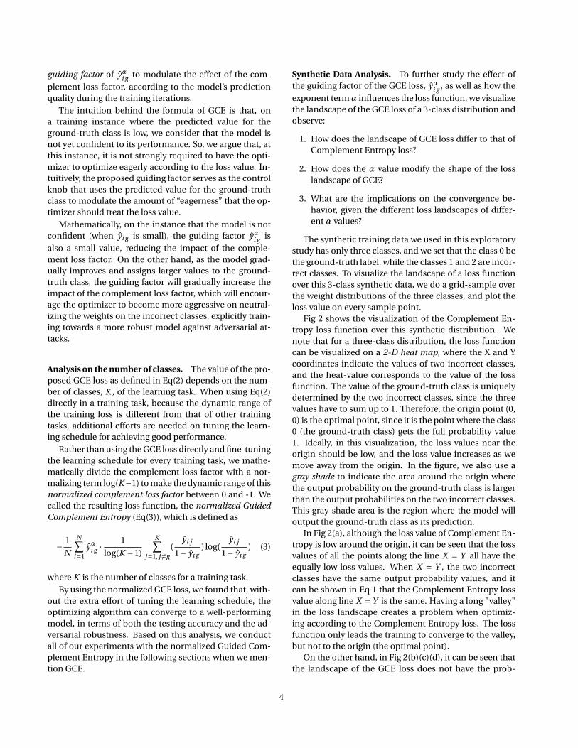
Fig 2 shows the visualization of the Complement En-tropy loss function over this synthetic distribution. Wenote that for a three-class distribution, the loss functioncan be visualized on a 2-D heat map, where the X and Ycoordinates indicate the values of two incorrect classes,and the heat-value corresponds to the value of the lossfunction. The value of the ground-truth class is uniquelydetermined by the two incorrect classes, since the threevalues have to sum up to 1. Therefore, the origin point (0,0) is the optimal point, since it is the point where the class0 (the ground-truth class) gets the full probability value1. Ideally, in this visualization, the loss values near theorigin should be low, and the loss value increases as wemove away from the origin. In the figure, we also use agray shade to indicate the area around the origin wherethe output probability on the ground-truth class is largerthan the output probabilities on the two incorrect classes.This gray-shade area is the region where the model willoutput the ground-truth class as its prediction.

In Fig 2(a), although the loss value of Complement En-tropy is low around the origin, it can be seen that the lossvalues of all the points along the line X = Y all have theequally low loss values. When X = Y , the two incorrectclasses have the same output probability values, and itcan be shown in Eq 1 that the Complement Entropy lossvalue along line X = Y is the same. Having a long "valley"in the loss landscape creates a problem when optimiz-ing according to the Complement Entropy loss. The lossfunction only leads the training to converge to the valley,but not to the origin (the optimal point).

On the other hand, in Fig 2(b)(c)(d), it can be seen thatthe landscape of the GCE loss does not have the prob-

4

(a) Complement Entropy (b) GCE with α= 1 (c) GCE with α= 1/3 (d) GCE with α= 1/10

Figure 2. Characteristics of GCE under different α values. Loss values are calculated assuming three classes, with class 0 being theground-truth and class 1 & 2 being incorrect classes. The X axis represents the predicted probability of class 1 and the Y axis for class2. The shaded area (at the bottom left of each sub-figure) represents the prediction being correct (i.e., ground-truth class receives thepredicted probability higher than class 1 or 2). Notice that in (a) and (d) the region of minimal loss (dark blue) does not overlap withthe shaded region, which is not ideal as the loss function couldn’t precisely reflect the prediction being correct. On the other hand,(b)(c) represent a preferred behavior of a loss function.

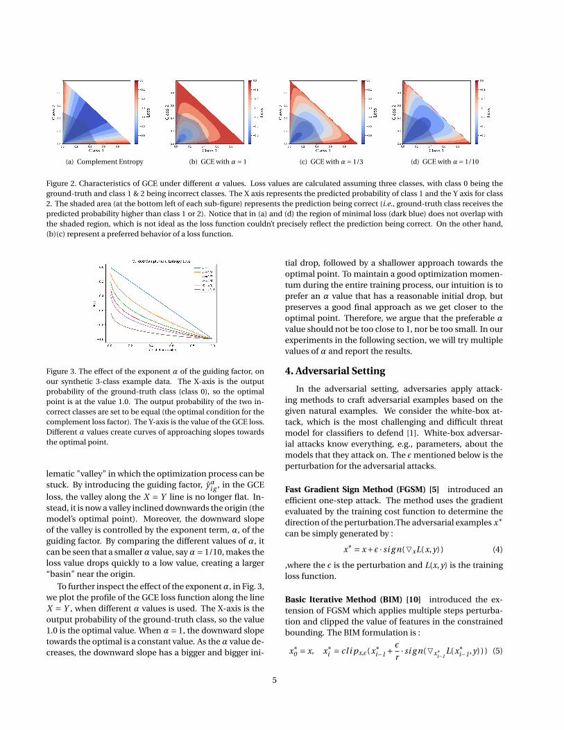
Figure 3. The effect of the exponent α of the guiding factor, onour synthetic 3-class example data. The X-axis is the outputprobability of the ground-truth class (class 0), so the optimalpoint is at the value 1.0. The output probability of the two in-correct classes are set to be equal (the optimal condition for thecomplement loss factor). The Y-axis is the value of the GCE loss.Different α values create curves of approaching slopes towardsthe optimal point.

lematic "valley" in which the optimization process can bestuck. By introducing the guiding factor, yαi g , in the GCE

loss, the valley along the X = Y line is no longer flat. In-stead, it is now a valley inclined downwards the origin (themodel’s optimal point). Moreover, the downward slopeof the valley is controlled by the exponent term, α, of theguiding factor. By comparing the different values of α, itcan be seen that a smallerα value, sayα= 1/10, makes theloss value drops quickly to a low value, creating a larger“basin" near the origin.

To further inspect the effect of the exponentα, in Fig. 3,we plot the profile of the GCE loss function along the lineX = Y , when different α values is used. The X-axis is theoutput probability of the ground-truth class, so the value1.0 is the optimal value. When α= 1, the downward slopetowards the optimal is a constant value. As theα value de-creases, the downward slope has a bigger and bigger ini-

tial drop, followed by a shallower approach towards theoptimal point. To maintain a good optimization momen-tum during the entire training process, our intuition is toprefer an α value that has a reasonable initial drop, butpreserves a good final approach as we get closer to theoptimal point. Therefore, we argue that the preferable αvalue should not be too close to 1, nor be too small. In ourexperiments in the following section, we will try multiplevalues of α and report the results.

4. Adversarial Setting

In the adversarial setting, adversaries apply attack-ing methods to craft adversarial examples based on thegiven natural examples. We consider the white-box at-tack, which is the most challenging and difficult threatmodel for classifiers to defend [1]. White-box adversar-ial attacks know everything, e.g., parameters, about themodels that they attack on. The ε mentioned below is theperturbation for the adversarial attacks.

Fast Gradient Sign Method (FGSM) [5] introduced anefficient one-step attack. The method uses the gradientevaluated by the training cost function to determine thedirection of the perturbation.The adversarial examples x∗can be simply generated by :

x∗ = x+ε · si g n(OxL(x,y) ) (4)

,where the ε is the perturbation and L(x,y) is the trainingloss function.

Basic Iterative Method (BIM) [10] introduced the ex-tension of FGSM which applies multiple steps perturba-tion and clipped the value of features in the constrainedbounding. The BIM formulation is :

x∗0 = x, x∗

i = cl i px,ε(x∗i−1+

ε

r· si g n(Ox∗i−1

L(x∗i−1,y) ) ) (5)

5

where the r is the number of iterations and clipx,ε(·) isthe clipping function to keep the value of features beingbounded.

Projected Gradient Descent (PGD) [14] proposed amore powerful adversary method which is the multi-stepvariant FGSMk. The process of crafting the adversarial ex-amples in PGD is similar to BIM. The difference is that thex∗

0 is a uniformly random point in `∞-ball around x.

Momentum Iterative Method (MIM) [4] integrated themomentum property into the iterative gradient-based at-tack to craft the adversarial examples. The method notonly stabilize the update directions during the iterativeprocess but also improve the situation about sticking inthe local maximum in BIM. The MIM formulation is:

gt =µ ·gt−1 +OxL(x∗

t−1,y)

‖OxL(x∗t−1,y)‖1

(6)

x∗t = cl i px,ε(x∗

t−1 +ε

r· si g n(gt ) ) (7)

where gt is the gradient which accumulating the velocityvector in the direction and µ is the decay factor.

Jacobian-based Saliency Map Attack (JSMA) [16] pro-posed the powerful target attack which can just perturbfewer pixels. The method identify the features that cansignificantly affect output classification by the evaluationof the saliency map. Through modifying the input fea-tures iterative, JSMA craft the adversarial example whichcause the model misclassified in specific targets.

Carlini & Wagner (C&W) [1] introduce a optimization-based attack and can effective defeat defensive distilla-tion [1]. To ensure the perturbation for images is avail-able, the method defines the box constraints to make thepixels value in a constrained bounding. They define:

x∗ = 1

2( tanh(w) +1) (8)

in terms of w and let 0 ≤ x∗ ≤ 1 to make the sample is validand optimize w with the formulation:

minw

‖1

2( tanh(w) +1) −x‖2

2 + c · f (1

2( tanh(w) +1)) (9)

where c is the constant. The f ( ·) is the objective function

f (x) = max(max{Zpre(x)i : i 6= y}−Zpre(x)i,−κ) (10)

where the κ is the confidence and Zpre(x)i is the modeloutput logits.

5. Experiments

We conduct experiments to demonstrate that:

1. Models trained with GCE can achieve better classifi-cation performance, compared to the baseline mod-els trained using the XE loss function.

2. In addition to achieving good classification perfor-mance on the natural, non-adversarial examples, themodels trained with GCE are also robust against sev-eral kinds of "white-box" adversarial attacks.

3. In the setting of "adversarial training", we show thatsubstituting the GCE loss function in the PGD adver-sarial training, the resulting models are more robustthan the previous results.

5.1. Performance on natural examples

In this section, we give experimental results show-ing that models trained using GCE, in the natural, non-adversarial setting, can outperform the previously re-ported best models trained using XE. Specifically, wecompared the model accuracy on several image classifica-tion datasets of different scales, ranging from MNIST [12],CIFAR10, CIFAR100 [8] and Tiny ImageNet2.

In our experiments, for each data set, we take the bestmodel previously published (the baseline model), andsubstitute the loss function from the original XE to theproposed GCE. For MNIST, we use the model Lenet-5 [12]with Adam Optimizer. For CIFAR10 and CIFAR100, we useResNet-56 [7]; while for Tiny ImageNet, it is trained withResNet-50. The ResNet-56 and ResNet-50 models weretrained following the standard settings described in [7].In details, the models were trained using SGD optimizerwith momentum of 0.9, and weight decay is set to be0.0001. The learning rate is set to start at 0.1, then is di-vided by 10 at the 100th and 150th epochs.

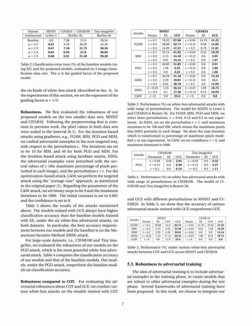
Table 2 compares the classification error rates of thebaseline models and those of GCE’s models. We foundthat the performance achieved by GCE’s models are usu-ally as good or outperforming the models from XE, whenthe guided factor, controlled by α, is appropriately cho-sen. For example, on Tiny ImageNet, our proposed modelachieves 38.56% error rate, atα= 1/3, which is better thanthe 39.54% error rate of the baseline model.

5.2. Robustness to White-box attacks

The main motivation of the proposed GCE loss, is totrain models that are robust to adversarial attacks. In thissection, we took the models that were trained above as de-scribed in Sec. 5.1, and evaluated their robustness against

2https://tiny-imagenet.herokuapp.com, a subset of Ima-geNet [3]

6

Dataset MNIST CIFAR10 CIFAR100 Tiny ImageNetArchitecture LeNet-5 ResNet-56 ResNet-50

Baseline 0.8 7.99 31.9 39.54α= 1/2 0.61 9.18 40.59 43.36α= 1/3 0.67 7.18 31.75 38.56α= 1/4 0.64 6.93 31.8 38.69α= 1/5 0.68 6.91 31.48 38.26

Table 2. Classification error rates (%) of the baseline models (us-ing XE) and the proposed models, evaluated on 4 image classi-fication data sets. The α is the guided factor of the proposedmodel.

the six kinds of white-box attack (described in Sec. 4). Inthe experiments of this section, we set the exponent of theguiding factor α= 1/3.

Robustness. We first evaluated the robustness of ourproposed models on the two smaller data sets, MNISTand CIFAR10. Following the preprocessing that is com-mon in previous work, the pixel values in both data setswere scaled to the interval [0,1]. For the iteration-basedattacks using gradients, e.g., FGSM, BIM, PGD and MIM,we crafted adversarial examples in the non-targeted way,with respect to the perturbation ε. The iterations are setto be 10 for BIM, and 40 for both PGD and MIM. Forthe iteration-based attack using Jacobian matrix, JSMA,the adversarial examples were perturbed with the sev-eral values of γ (the maximum percentage of pixels per-turbed in each image), and the perturbation ε=1. For theoptimization-based attack, C&W, we perform the targetedattack using the "average case" approach, as mentionedin the original paper [1]. Regarding the parameters of theC&W attack, we set binary steps to be 9 and the maximumiterations to be 1000. The initial constant is set to 0.001and the confidence is set to 0.

Table 3 shows the results of the attacks mentionedabove. The models trained with GCE always have higherclassification accuracy than the baseline models trainedwith XE, under the six white-box adversarial attacks, onboth datasets. In particular, the best accuracy improve-ment between our models and the baseline is on the Mo-mentum Iterative Method (MIM) attack.

For large-scale datasets, i.e., CIFAR100 and Tiny Ima-geNet, we evaluated the robustness of our models on thePGD attack, which is the most powerful white-box adver-sarial attack. Table 4 compares the classification accuracyof our models and that of the baseline models. Our mod-els, under the PGD attack, outperform the baseline mod-els on classification accuracy.

Robustness compared to COT. For evaluating the ad-versarial robustness about COT and GCE, we conduct var-ious white-box attacks on the models trained with COT

AttacksMNIST CIFAR10

Param. XE GCE Param. XE GCE

FGSMε= 0.1ε= 0.2ε= 0.3

78.3238.8814.99

87.6662.7447.21

ε= 0.04ε= 0.12ε= 0.2

14.769.588.78

41.2214.8211.81

BIMε= 0.1ε= 0.2ε= 0.3

53.142.150.01

61.9234.4933.45

ε= 0.04ε= 0.12ε= 0.2

0.250.00.0

19.593.031.97

PGDε= 0.1ε= 0.2ε= 0.3

46.851.580.0

51.859.552.22

ε= 0.04ε= 0.12ε= 0.2

0.00.00.0

5.911.891.66

MIMε= 0.1ε= 0.2ε= 0.3

48.282.290.01

61.1839.8138.78

ε= 0.04ε= 0.12ε= 0.2

0.00.00.0

15.4413.1

12.69

JSMAγ= 0.25γ= 0.5

1.530.1

26.2417.26

γ= 0.07γ= 0.14

1.090.14

18.7210.94

C&W c = 0. 0.0 25.6 c = 0. 0.0 0.8

Table 3. Performance (%) on white-box adversarial attacks withwide range of perturbations. The model for MNIST is Lenet-5and CIFAR10 is Resnet-56. For FGSM, BIM, PGD and MIM, weselect three perturbations, ε = 0.04, 0.12 and 0.2 in our exper-iment. In JSMA, we set the perturbation ε = 1. and maximumiterations to be 100 and 200, which means the maximum pixelsthat JSMA purturbs in each image. We show the max iterationwhich is transformed to percentage of maximum pixels modi-fied γ in our experiment. In C&W, we set confidence c = 0. andmaximum iterations is 1000.

AttacksCIFAR100 Tiny ImageNet

Parameter XE GCE Parameter XE GCE

PGDε= 0.04ε= 0.12ε= 0.2

0.040.00.0

2.940.460.19

ε= 0.04ε= 0.12ε= 0.2

0.00.00.0

9.524.271.11

Table 4. Performance (%) on white-box adversarial attacks withwide range of perturbations in CIFAR100. The model of CI-FAR100 and Tiny ImageNet is Resnet-56.

and GCE with different perturbations in MNIST and CI-FAR10. In Table 5, we show that the accuracy of variousadversarial attacks trained with GCE outperforms COT.

AttacksMNIST CIFAR 10

Param. XE COT GCE Param. XE COT GCEFGSM ε = 0.2 38.88 51.8 62.74 ε = 0.04 14.76 33.62 41.22BIM ε = 0.2 2.15 4.35 34.49 ε = 0.04 0.25 7.49 19.59MIM ε = 0.2 2.29 4.26 39.81 ε = 0.04 0.0 0.0 15.44JSMA γ = 0.25 1.53 11.13 26.24 γ = 0.07 1.09 8.25 18.72C&W c = 0 0.0 11.9 25.6 c = 0 0.0 0.0 0.8

Table 5. Performance (%) under various white-box adversarialattacks between COT and GCE across MNIST and CIFAR10.

5.3. Robustness to adversarial training

The idea of adversarial training is to include adversar-ial examples in the training phase, to create models thatare robust to other adversarial examples during the testphase. Several frameworks of adversarial training havebeen proposed. In this work, we choose to integrate our

7

proposed GCE loss function in the Projected Gradient De-scent (PGD) adversarial training, since the PGD attack isconsidered an universal one, among all of the first-orderadversarial attacks [14]. We show that the resulting mod-els from this integration are more robust than the onestrained using the original PGD approach.

The PGD adversarial training uses a min-max objectivefunction to accomplish adversarial training:

minθ

ρ(θ), where ρ(θ) = Ex,y∼D

[maxδ

L(θ, x +δ, y)]. (11)

, where D is the data distribution over pairs of trainingsample x and label y. The loss function L(·) is the XE loss.In Eq(11), the inner maximization problem is for craftingtraining adversarial examples to induce maximum lossvalues, while the outer minimization problem is for build-ing a classification model, ρ(·), to minimize the adversar-ial loss by the universal adversary. One typical approachfor optimizing this min-max objective is through an itera-tive algorithm.

In the original work, the loss function for the innermaximization and that for the outer minimization are thesame, which is the XE loss. In our work, we keep the lossfunction for the inner maximization intact as the XE loss,because it has been proved that the PGD framework gen-erates the optimal adversarial examples, among all first-order adversarial attacks, when using the XE loss. On theother hand, for the outer minimization, that is, the train-ing of the classification model, we replace the XE loss withour proposed GCE loss. This way of integration is similarto other previous work [19] that also keeps the XE as theloss function of the inner maximization problem.

In our setup, we use GCE (α= 1/3) as the loss functionfor the Empirical Risk Minimization (ERM) [22] instead oforiginal XE in Eq(11). Then, to compare the robustnessof the models generated using our setup, with the mod-els trained using the original setup, we attack both thesemodels using the PGD white-box (with respect to the XEloss) adversarial attack.

In our experiments, the minimization models we usedare the baseline models as described in the previoussections, i.e., LeNet or Resnet, for their correspondingdatasets. Table 6 shows the comparison results on MNISTand CIFAR10 datasets. More specifically, in our experi-ments, we use the same settings of the iterative optimiza-tion as used in the previous work [14], to conduct the ad-versarial training and adversarial attacks: on MNIST, wedo 40 iterations of crafting adversarial examples duringtraining; at the testing phase, 100 iterations are used toapply the PGD attack. On CIFAR10, 10 iterations of ad-versarial training are used, and the adversarial attacks areconducted with 40 iterations. We demonstrate better ro-bustness while using GCE loss for the outer minimization.

AttacksMNIST CIFAR10

perturbation XE GCE perturbation XE GCE

PGD ε= 0.3 83.67 83.85ε= 0.04ε= 0.08

41.5012.93

41.5713.16

Table 6. Performance (%) of Adversarial training under PGD ad-versarial attacks on MNIST and CIFAR10.

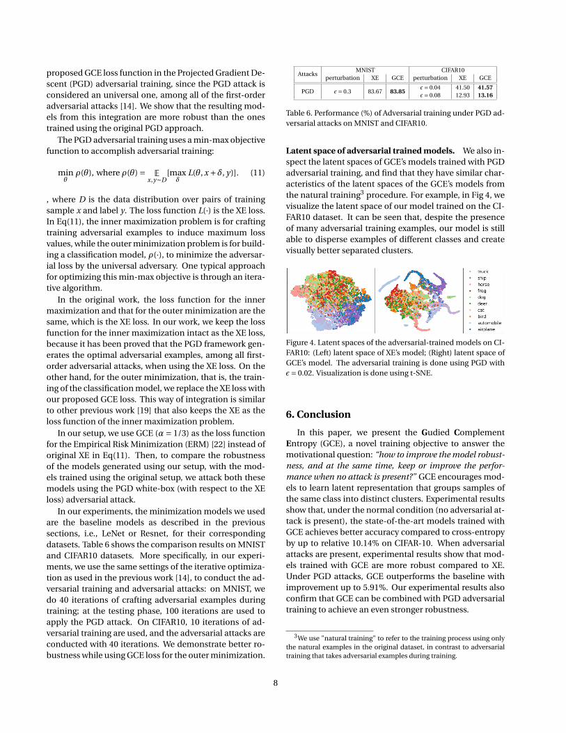
Latent space of adversarial trained models. We also in-spect the latent spaces of GCE’s models trained with PGDadversarial training, and find that they have similar char-acteristics of the latent spaces of the GCE’s models fromthe natural training3 procedure. For example, in Fig 4, wevisualize the latent space of our model trained on the CI-FAR10 dataset. It can be seen that, despite the presenceof many adversarial training examples, our model is stillable to disperse examples of different classes and createvisually better separated clusters.

Figure 4. Latent spaces of the adversarial-trained models on CI-FAR10: (Left) latent space of XE’s model; (Right) latent space ofGCE’s model. The adversarial training is done using PGD withε= 0.02. Visualization is done using t-SNE.

6. Conclusion

In this paper, we present the Gudied ComplementEntropy (GCE), a novel training objective to answer themotivational question: “how to improve the model robust-ness, and at the same time, keep or improve the perfor-mance when no attack is present?” GCE encourages mod-els to learn latent representation that groups samples ofthe same class into distinct clusters. Experimental resultsshow that, under the normal condition (no adversarial at-tack is present), the state-of-the-art models trained withGCE achieves better accuracy compared to cross-entropyby up to relative 10.14% on CIFAR-10. When adversarialattacks are present, experimental results show that mod-els trained with GCE are more robust compared to XE.Under PGD attacks, GCE outperforms the baseline withimprovement up to 5.91%. Our experimental results alsoconfirm that GCE can be combined with PGD adversarialtraining to achieve an even stronger robustness.

3We use "natural training" to refer to the training process using onlythe natural examples in the original dataset, in contrast to adversarialtraining that takes adversarial examples during training.

8

References

[1] Nicholas Carlini and David A. Wagner. Towards evaluatingthe robustness of neural networks. In IEEESSP’17, 2017.

[2] Hao-Yun Chen, Pei-Hsin Wang, Chun-Hao Liu, Shih-ChiehChang, Jia-Yu Pan, Yu-Ting Chen, Wei Wei, and Da-ChengJuan. Complement objective training. In ICLR’19, 2019.

[3] Jia Deng, Wei Dong, Richard Socher, Li jia Li, Kai Li, andLi Fei-fei. ImageNet: A large-scale hierarchical imagedatabase. In CVPR’09, 2009.

[4] Yinpeng Dong, Fangzhou Liao, Tianyu Pang, Hang Su, JunZhu, Xiaolin Hu, and Jianguo Li. Boosting adversarial at-tacks with momentum. In CVPR’18, 2018.

[5] Ian Goodfellow, Jonathon Shlens, and Christian Szegedy.Explaining and harnessing adversarial examples. InICLR’15, 2015.

[6] Ian J. Goodfellow, Jean Pouget-Abadie, Mehdi Mirza, BingXu, David Warde-Farley, Sherjil Ozair, Aaron Courville,and Yoshua Bengio. Generative Adversarial Networks. InICLR’14, 2014.

[7] Kaiming He, Xiangyu Zhang, Shaoqing Ren, and Jian Sun.Deep residual learning for image recognition. In CVPR’16,2016.

[8] Alex Krizhevsky. Learning multiple layers of features fromtiny images. Technical report, 2009.

[9] Alex Krizhevsky, Ilya Sutskever, and Geoffrey E Hinton. Im-agenet classification with deep convolutional neural net-works. In NIPS’12, 2012.

[10] Alexey Kurakin, Ian J. Goodfellow, and Samy Bengio. Adver-sarial examples in the physical world. In ICLR’17 Workshop,2017.

[11] Alexey Kurakin, Ian J. Goodfellow, and Samy Bengio. Ad-versarial machine learning at scale. In ICLR’17, 2017.

[12] Y. Lecun, L. Bottou, Y. Bengio, and P. Haffner. Gradient-based learning applied to document recognition. Proceed-ings of the IEEE, 1998.

[13] Tsung-Yi Lin, Michael Maire, Serge J. Belongie, Lubomir D.Bourdev, Ross B. Girshick, James Hays, Pietro Perona, DevaRamanan, Piotr Dollár, and C. Lawrence Zitnick. MicrosoftCOCO: common objects in context. In ECCV’14, 2014.

[14] Aleksander Madry, Aleksandar Makelov, Ludwig Schmidt,Dimitris Tsipras, and Adrian Vladu. Towards deep learningmodels resistant to adversarial attacks. In ICLR’18, 2018.

[15] Preetum Nakkiran. Adversarial robustness may be at oddswith simplicity. arXiv preprint arXiv:1901.00532, 2019.

[16] Nicolas Papernot, Patrick McDaniel, Somesh Jha, MattFredrikson, Z. Berkay Celik, and Ananthram Swami. Thelimitations of deep learning in adversarial settings. In IEEEEuropean Symposium on Security and Privacy, 2016.

[17] Nicolas Papernot and Patrick D. McDaniel. Extending de-fensive distillation. arXiv preprint arXiv:1705.05264, 2017.

[18] Nicolas Papernot, Patrick D. McDaniel, Xi Wu, Somesh Jha,and Ananthram Swami. Distillation as a defense to adver-sarial perturbations against deep neural networks. In IEEESymposium on Security and Privacy, 2015.

[19] Aditi Raghunathan, Jacob Steinhardt, and Percy Liang. Cer-tified defenses against adversarial examples. In ICLR’18,2018.

[20] Florian Tramèr, Alexey Kurakin, Nicolas Papernot, IanGoodfellow, Dan Boneh, and Patrick McDaniel. Ensem-ble adversarial training: Attacks and defenses. In ICLR’18,2018.

[21] Dimitris Tsipras, Shibani Santurkar, Logan Engstrom,Alexander Turner, and Aleksander Madry. Robustness maybe at odds with accuracy. In ICLR’19, 2019.

[22] Vladimir N Vapnik. An overview of statistical learning the-ory. IEEE transactions on neural networks, 1999.

[23] Tsui-Wei Weng, Huan Zhang, Pin-Yu Chen, Jinfeng Yi,Dong Su, Yupeng Gao, Cho-Jui Hsieh, and Luca Daniel.Evaluating the robustness of neural networks: An extremevalue theory approach. In ICLR’18, 2018.

9