Di r ecci ó n:Di r ecci ó n: Biblioteca Central Dr. Luis F. Leloir, Facultad de Ciencias Exactas y Naturales, Universidad de Buenos Aires. Intendente Güiraldes 2160 - C1428EGA - Tel. (++54 +11) 4789-9293

Co nta cto :Co nta cto : digital@bl.fcen.uba.ar

Tesis Doctoral

Implicitación de aplicacionesImplicitación de aplicacionesracionalesracionales

Botbol, Nicolás S.

2010

Este documento forma parte de la colección de tesis doctorales y de maestría de la BibliotecaCentral Dr. Luis Federico Leloir, disponible en digital.bl.fcen.uba.ar. Su utilización debe seracompañada por la cita bibliográfica con reconocimiento de la fuente.

This document is part of the doctoral theses collection of the Central Library Dr. Luis FedericoLeloir, available in digital.bl.fcen.uba.ar. It should be used accompanied by the correspondingcitation acknowledging the source.

Cita tipo APA:

Botbol, Nicolás S.. (2010). Implicitación de aplicaciones racionales. Facultad de CienciasExactas y Naturales. Universidad de Buenos Aires.

Cita tipo Chicago:

Botbol, Nicolás S.. "Implicitación de aplicaciones racionales". Facultad de Ciencias Exactas yNaturales. Universidad de Buenos Aires. 2010.

UNIVERSIDAD DE BUENOS AIRES UNIVERSITE PIERRE ET MARIE CURIEFacultad de Ciencias Exactas y Naturales Sciences Mathematiques de Paris Centre

Departamento de Matematica Institut de Mathematiques de Jussieu

IMPLICITACION DE APLICACIONES RACIONALES

Tesis presentada para optar al tıtulo de

Doctor de la Universidad de Buenos Aires

en el area Ciencias Matematicas y

Doctor de la Universite Pierre et Marie Curie,

Especialidad Ecole doctorale Sciences Mathematiques de Paris Centre.

Nicolas S. Botbol

Directores de tesis: Dr. Marc Chardin

Dra. Alicia Dickenstein

Consejero de estudios: Dra. Alicia Dickenstein

Buenos Aires, 2010.

IMPLICITIZATION OF RATIONAL MAPS.

Motivated by the interest in computing explicit formulas for resultants anddiscriminants initiated by Bezout, Cayley and Sylvester in the eighteenthand nineteenth centuries, and emphasized in the latest years due to theincrease of computing power, we focus on the implicitization of hypersurfacesin several contexts. Implicitization means, given a rational map f : An−1 99K

An, to compute an implicit equation H of the closed image im(f). This isa classical problem and there are numerous approaches to its solution (cf.[SC95] and [Cox01]). However, it turns out that the implicitization problemis computationally difficult.

Our approach is based on the use of linear syzygies by means of ap-proximation complexes, following [BJ03], [BC05], and [Cha06], where theydevelop the theory for a rational map f : Pn−1 99K Pn. Approximation com-plexes were first introduced by Herzog, Simis and Vasconcelos in [HSV83b]almost 30 years ago.

The main obstruction for this approximation complex-based methodcomes from the bad behaviour of the based locus of f . Thus, it is natu-ral to try different compatifications of An−1, that are better suited to themap f , in order to avoid unwanted base points. With this purpose, in thisthesis we study toric compactifications T for An−1. First, we view T em-bedded in a projective space. Furthermore, we compactify the codomaininside (P1)n, to deal with the case of different denominators in the rationalfunctions defining f . We also approach the implicitization problem consid-ering the toric variety T defined by its Cox ring, without any particularprojective embedding. In all this cases, we blow-up the base locus of themap and we approximate the Rees algebra ReesA(I) of this blow-up by thesymmetric algebra SymA(I). We provide resolutions Z• for SymA(I), suchthat det((Z•)ν) gives a multiple of the implicit equation, for a graded strandν ≫ 0. Precisely, we give specific bounds ν on all these settings which de-pend on the regularity of SymA(I). We also give a geometrical interpretationof the possible other factors appearing on det((Z•)ν).

Starting from the homogeneous structure of the Cox ring of a toric va-riety, graded by the divisor class group of T , we give a general definitionof Castelnuovo-Mumford regularity for a polynomial ring R over a commu-tative ring k, graded by a finitely generated abelian group G, in terms ofthe support of some local cohomology modules. As in the standard case, fora G-graded R-module M and an homogeneous ideal B of R, we relate thesupport of H i

B(M) with the support of TorRj (M, k).

IMPLICITIZATION D’APPLICATIONS RATIONNELLES.

Motives par la recherche de formules explicites pour les resultants et lesdiscriminants, qui remonte au moins aux travaux de Bezout, Cayley etSylvester au XVIIIeme et XIXeme siecles et a donne lieu a de nouveauxdeveloppements dans les dernieres annees en raison de l’augmentation de lapuissance de calcul, on se concentre sur l’implicitisation des hypersurfacesdans plusieurs contextes. Implicitisation signifie calculer une equation im-plicite H de l’image fermee im(f), etant donne une application rationnellef : A(n−1) 99K An. C’est un probleme classique et il y a de nombreusesapproches (cf. [SC95] et [Cox01]). Toutefois, il s’avere que le problemed’implicitisation est difficile du point de vue du calcul.

Notre approche est basee sur l’utilisation des syzygies lineaires au moyende complexes d’approximation, en suivant [BJ03], [BC05], et [Cha06], ou ilsdeveloppent la theorie pour une application rationnelle f : P(n−1) 99K Pn.Les complexes d’approximation ont d’abord ete introduits par Herzog, Simiset Vasconcelos dans [HSV83b] il y a presque 30 ans.

L’obstruction principale de la methode des complexes d’approximationvient du mauvais comportement du lieu base de f . Ainsi, il est natureld’essayer differentes compatifications de A(n−1), qui sont mieux adaptes af , afin d’eviter des points base non desires. A cet effet, dans cette theseon etudie des compactifications toriques T de A(n−1). Tout d’abord, onconsidere T plongee dans un espace projectif. En outre, on compactifie lecodomaine dans (P1)n, pour faire face aux cas des denominateurs differentsdans les fonctions rationnelles qui definissent f . On a egalement abordele probleme implicitisation lorsque la variete torique T est definie par sonanneau de Cox, sans un plongement projectif particulier. Dans tous ces cas,on eclate le lieu base de f et on approche l’algebre de Rees ReesA(I) parl’algebre symetrique SymA(I). On fournit des resolutions Z• de SymA(I),telle que det((Z•)ν) donne un multiple de l’equation implicite, pour ν ≫0. Precisement, on donne des bornes specifiques ν dans tous ces cas quidependent de la regularite de SymA(I). On donne aussi une interpretationgeometrique des autres facteurs possibles qui apparaissent dans det((Z•)ν).

Motive par la structure homogene de l’anneau Cox d’une variete torique,graduee par le groupe de classes de diviseurs de T , on donne unedefinition generale de regularite de Castelnuovo-Mumford pour un anneaude polynomes R sur un anneau commutatif k, gradue par un groupe abeliende rang fini G, en termes du support de certains modules de cohomologielocale. Comme dans le cas standard, pour un R-module M G-gradue etun ideal homogene B de R, on lie le support de H i

B(M) avec le support deTorRj (M, k).

5

IMPLICITACION DE APLICACIONES RACIONALES.

Motivados por el interes en el calculo de formulas explıcitas para resul-tantes y discriminantes que viene desde Bezout, Cayley y Sylvester en lossiglos XVIII y XIX, y enfatizado en los ultimos anos por el aumento delpoder de computo, nos concentramos en la implicitacion de hipersuperficiesen diversos contextos. Por implicitacion entendemos que, dada una apli-cacion racional f : An−1 99K An, calculamos una ecuacion implıcita H dela clausura de la imagen im(f). Este es un problema clasico con numerosasaproximaciones para su solucion (cf. [SC95] y [Cox01]). A pesar de esto, elproblema de implicitacion es computacionalmente difıcil.

Nuestro enfoque se basa en el uso de sicigias lineales mediante complejosde aproximacion, siguiendo [BJ03], [BC05], y [Cha06], donde los autoresdesarrollan la teorıa para una aplicacion racional f : Pn−1 99K Pn. Loscomplejos de aproximacion fueron introducidos por primera vez por Herzog,Simis y Vasconcelos en [HSV83b] hace casi 30 anos.

La principal obstruccion para este metodo basado en complejos de aprox-imacion proviene del mal comportamiento del lugar base de f . Luego, esnatural buscar diferentes compactificaciones de An−1, que esten mejor adap-tadas a la aplicacion f , con el fin de evitar puntos base no deseados. Coneste objetivo, en esta tesis estudiamos compactificaciones toricas T paraAn−1. Primero, vemos a T sumergida en un espacio proyectivo. Mas aun,compactificamos el codominio en (P1)n, para tratar el caso en que las fun-ciones racionales que definen a f tengan diferentes denominadores. Tambienabordamos el problema de implicitacion considerando la variedad torica Tdefinida por su anillo de Cox, sin una inmersion proyectiva particular. Entodos estos casos, explotamos el lugar base de f y aproximamos al algebrade Rees de este blow-up ReesA(I), mediante el algebra simetrica SymA(I).Proveemos resoluciones Z• de ReesA(I) tales que det((Z•)ν) da un multiplode la ecuacion implıcita, para una capa graduada ν ≫ 0. Mas precisamente,en todos estos casos damos cotas para ν que dependen de la regularidad deSymA(I). Tambien damos una interpretacion geometrica para los posiblesfactores extras que aparecen en det((Z•)ν).

Comenzando desde la estructura homegenea del anillo de Cox de la var-iedad torica, graduado por el grupo de clases de divisores de T , damos unadefinicion general de la regularidad de Castelnuovo-Mumford para anillos depolinomios R sobre un anillo conmutativo k, graduado por un grupo abelianoG finitamente generado, en termino de los soportes de algunos modulos decohomologıa local. Tal como en el caso estandar, dado un R-modulo M G-graduado y un ideal homogeneo B de R, relacionamos el soporte de H i

B(M)con el soporte de TorRj (M, k).

7

I would like to thank

a mi directora Alicia et a mon directeur Marc, for allthey have done for me, teaching, helping, suggesting. Itwas simultaneously a pleasure and a honor;

a mis amigos de la facultad, por acompanarme y faci-litarme el trabajo durante estos anos, sin su ayuda estetrabajo no hubiera sido posible. Al resto de mis amigos,por su apoyo incondicional. A Ale;

a mes amis conus en France, car vous avez faites qu’etreloin de chez moi soit agreable. Avec qui j’ai bien travailleet amuse;

to all mathematicians that helped me constructing whatI have done in this science;

A mi familia, a mis padres y a mi hermana. A Flor.

Gracias.

9

Introduction

The interest in computing explicit formulas for resultants and discriminants goes back toBezout, Cayley, Sylvester and many others in the eighteenth and nineteenth centuries. Ithas been emphasized in the latest years due to the increase of computing power. Undersuitable hypotheses, resultants give the answer to many problems in elimination theory,including the implicitization of rational maps. In turn, both resultants and discriminantscan be seen as the implicit equation of a suitable map (cf. [DFS07]). Lately, rationalmaps appeared in computer-engineering contexts, mostly applied to shape modelingusing computer-aided design methods for curves and surfaces.

Rational algebraic curves and surfaces can be described in several different ways, themost common being parametric and implicit representations. Parametric representa-tions describe the geometric object as the image of a rational map, whereas implicitrepresentations describe it as the set of points verifying a certain algebraic condition,e.g. as the zeros of a polynomial equation. Both representations have a wide range ofapplications in Computer Aided Geometric Design (CAGD), and depending on the prob-lem one needs to solve, one or the other might be better suited. It is thus interesting tobe able to pass from parametric representations to implicit equations. This is a classicalproblem and there are numerous approaches to its solution (a good historical overviewon this subject can be seen in [SC95] and [Cox01]). However, it turns out that theimplicitization problem is computationally difficult.

A promising alternative suggested in [BD07] is to compute a so-called matrix represen-tation instead, which is easier to compute but still shares some of the advantages of theimplicit equation. Let K be a field. For a given hypersurface H ⊂ Pn, a matrix M withentries in the polynomial ring K[X0, . . . , Xn] is called a representation matrix of H if itis generically of full rank and if the rank of M evaluated in a point of Pn drops if andonly if the point lies on H (see Chapter 3, also cf. [BDD09]). Equivalently, a matrixM represents H if and only if the greatest common divisor of all its minors of maximalsize is a power of the homogeneous implicit equation F ∈ K[X0, . . . , Xn] of H .

In the case of a planar rational curve C given by a parametrization of the form A1f

99K A2,

s 7→(f1(s)f3(s)

, f2(s)f3(s)

), where fi ∈ K[s] are coprime polynomials of degree d and K is a field,

a linear syzygy (or moving line) is a linear relation on the polynomials f1, f2, f3, i.e. alinear form L = h1X1 + h2X2 + h3X3 in the variables X1, X2, X3 and with polynomial

11

coefficients hi ∈ K[s] such that∑

i=1,2,3 hifi = 0. We denote by Syz(f) the set of allthose linear syzygy forms and for any integer ν the graded part Syz(f)ν of syzygies ofdegree at most ν. To be precise, one should homogenize the fi with respect to a newvariable and consider Syz(f) as a graded module here. It is obvious that Syz(f)ν is afinite-dimensional K-vector space of dimension k = k(ν), obtained by solving a linearsystem. Let L1, . . . , Lk be a basis of Syz(f)ν . If Li =

∑|α|=ν s

αLi,α(X1, X2, X3), we

define the matrix Mν = (Li,α)1≤i≤k,|α|=ν , that is, the coefficients of the Li with respectto a K-basis of K[s]ν form the columns of the matrix. Note that the entries of thismatrix are linear forms in the variables X1, X2, X3 with coefficients in the field K. LetF denote the homogeneous implicit equation of the curve and deg(f) the degree of theparametrization as a rational map. Intuitively, deg(f) measures how many times thecurve is traced. It is known that for ν ≥ d−1, the matrix Mν is a representation matrix;more precisely: if ν = d − 1, then Mν is a square matrix, such that det(Mν) = F deg(f).Also, if ν ≥ d, then Mν is a non-square matrix with more columns than rows, such thatthe greatest common divisor of its minors of maximal size equals F deg(f). In other words,one can always represent the curve as a square matrix of linear syzygies. One could nowactually calculate the implicit equation. We overview this subject more widely in Section1.7.1.

For surfaces, matrix representations have been studied in [BDD09] for the case of 2-dimensional projective toric varieties, and we will analyze it in detail in Chapter 3.Previous work had been done in this direction, with two main approaches: One allowsthe use of quadratic syzygies (or higher-order syzygies) in addition to the linear syzygies,in order to be able to construct square matrices, the other one only uses linear syzygiesas in the curve case and obtains non-square representation matrices.

The first approach using linear and quadratic syzygies (or moving planes and quadrics)has been treated in [Cox03a] for base-point-free homogeneous parametrizations and somegenericity assumptions, when T = P2. The authors of [BCD03] also treat the case oftoric surfaces in the presence of base points. In [AHW05], square matrix representationsof bihomogeneous parametrizations, i.e. T = P1 × P1, are constructed with linear andquadratic syzygies, whereas [KD06] gives such a construction for parametrizations overtoric varieties of dimension 2. The methods using quadratic syzygies usually requireadditional conditions on the parametrization and the choice of the quadratic syzygies isoften not canonical.

The second approach, developed in more detail in Section 1.7.2, even though it does notproduce square matrices, has certain advantages, in particular in the sparse setting thatwe present. In previous publications, this approach with linear syzygies, which relies onthe use of the so-called approximation complexes has been developed in the case T = Pn,see for example [BJ03], [BC05], and [Cha06], and T = P1 × P1 in [BD07] for bihomo-geneous parametrizations of degree (d, d). However, for a given affine parametrizationf , these two varieties T are not necessarily the best choice of a compactification, since

12

they do not always reflect well the combinatorial structure of the polynomials definingthe parametrization. We extend the method to a much larger class of varieties, namelytoric varieties of dimension 2 (cf. [BDD09], see also 3.4). We show that it is possibleto choose a “good” toric compactification of (A∗)2 depending on the input polynomials,which makes the method applicable in cases where it failed over P2 or P1 × P1. Also, itis significantly more efficient, leading to smaller representation matrices.

Later, in [Bot10], see Chapter 3, we gave different compactifications for the domainand the codomain of an affine rational map f that parametrizes a hypersurface in anydimension and we show that the closure of the image of this map (with possibly someother extra hypersurfaces) can be represented by a matrix of linear syzygies, relaxingthe hypothesis on the base locus. More generally, we compactify An−1 into an (n −1)-dimensional projective arithmetically Cohen-Macaulay subscheme of some PN . Westudied one particular interesting compactification of An−1 which is the toric varietyassociated to the Newton polytope of the polynomials defining f .

In [Bot09b] and [Bot10] we considered a different compactifications for the codomainof f , (P1)n as is detailed in Chapter 4. We study the implicitization problem in thissetting. This new perspective allow to deal with parametric rational maps with differentdenominators. Precisely, if are given f = (f1

g1, . . . , fn

gn) : An−1 99K An, we can naturally

consider a map φ = ((f1 : g1) × · · · (fn : gn)) : Pn−1 99K (P1)n (cf. [Bot09b]). As wehave remarked before, Pn−1 need not be the best compactification of the domain of f ,thus, in [Bot10] we extended this method the setting φ : T 99K (P1)n where T is anyarithmetically Cohen-Macaulay closed subscheme of some PN . In this last context, wegave sufficient conditions, in terms of the nature of the base locus of the map, for gettinga matrix representation of its closed image, without involving extra hypersurfaces (cf.Chapter 4).

In order to avoid a particular embedding of T in PN , we focused on the study of implicit-ization problem for toric varieties given by its Cox ring (see Section 2.4 or [Cox95]). Thisleaded to adapting the technique based on approximation complexes for more generalgraded rings and modules. In Chapter 6 we give a definition of Castelnuovo-Mumford

regularity for a commutative ring R graded by a finitely generated abelian group G, interms of the support of some local cohomology modules. A very interesting example isthat of Cox rings of toric varieties, where the grading is given by the Chow group ofthe variety acting on a polynomial ring. Thus, this allows to study the implicitizationproblem for general arithmetically Cohen Macaulay toric varieties without the need ofan embedding, as we do in Chapter 7.

13

Organization

Ch. 1: Preliminaries on elimination theory and approximation complexes.

Ch. 2: Preliminaries on toric varieties.

Ch. 3: Implicitization for ϕ : T 99K Pn, by means of an embedding T ⊂ PN .

Ch. 4: Implicitization for φ : T 99K (P1)n, by means of an embedding T ⊂ PN .

Ch. 5: Algorithmic approach for Chapters 3 and 4, and examples

Ch. 6: Castelnuovo-Mumford regularity for G-graded rings, for G abelian group.

Ch. 7: Implicitization φ : T 99K Pn, where T is defined by the Cox ring.

Ch. 8: Algorithm for ϕ : T 99K P3 following 3.

Ch. 9: Algorithm for ϕ : T 99K P3 following 7.

Chapter 1 Chapter 2

Chapter 3

Chapter 5

Chapter 4 Chapter 6

Chapter 7

Chapter 8 Chapter 9

In Chapter 1 we give a fast overview of the original technique of computing implicitequations for projective rational maps by means of approximation complexes. Indeed, weintroduce in Section 1.5 the notion of approximation complexes and of blow-up algebrasin Section 1.3, and we give basic results that we will use later in this thesis. As it wasmentioned, this approach with linear syzygies was first formulated for this purpose in[BJ03] an later improved in [BC05], [Cha06] and [BCJ09]. We give a more detailedoutline of this method in Section 1.7.2.

Chapter 2 is mainly devoted to give an introduction to toric varieties. We recall someresults that we will need later, in order to generalize the implicitization methods for toriccompactifications. We develop this idea in Chapters 3, 4 and 7.

14

In Chapters 3 and 4 we adapt the method of approximation complexes to computing animplicit equation of a parametrized hypersurface, focusing on different compactificationsof the domain T and of the codomain (Pn and (P1)n). We will always assume thatT is a (n − 1)-dimensional closed subscheme of PN with graded and Cohen-Macaulayn-dimensional coordinate ring A.

In Chapter 3, we focus on the implicitization problem for a rational map ϕ : T 99K Pn

defined by n+1 polynomials of degree d. We extend the method to maps defined over an(n − 1)-dimensional Cohen-Macaulay closed scheme T , embedded in PN , emphasizingthe case where T is a toric variety. We show that we can relax the hypotheses on thebase locus by admitting it to be a zero-dimensional almost locally complete intersectionscheme. Implicitization in codimension one is well adapted in this case, as is shown inSection 3.2 and 3.3, following the spirit of many papers in this subject: [BJ03], [BCJ09],[BD07], [BDD09] and [Bot09b].

In order to consider more general parametrizations given by rational maps of the formf = (f1

g1, . . . , fn

gn) with different denominators g1, . . . , gn, we develop in Chapter 4 the

study of the (P1)n compactification of the codomain. With this approach, we studyfollowing [Bot09b] and [Bot10], the method of implicitization of projective hypersurfacesembedded in (P1)n. As in Chapters 1 and 3, we compute the implicit equation as thedeterminant of a complex which coincides with the gcd of the maximal minors of the lastmatrix of the complex, and we make deep analysis of the geometry of the base locus.

In Chapter 5 we exemplify the results of Chapters 3 and 4, and we study in a morecombinatorial fashion the size of the matrices obtainned. We analyze, in both settings,how taking an homothety of the Newton polytope N (f) can modify the size of thematrices Mν . We present several examples comparing our results with the previousones. First, we show in a very sparse setting the advantage of not considering thehomogeneous compactification of the domain when denominators are very different. Weextend in the second example this idea to the case of a generic affine rational map indimension 2 with fixed Newton polytope. In the last example we give, for a parametrizedtoric hypersurface of (P1)n, a detailed analysis of the relation between the nature of thebase locus of a map and the extra factors appearing in the computed equation. We finishthis section by giving an example of how the developed technique can be applied to thecomputation of sparse discriminants.

In order to avoid a particular embedding of T in PN , we focus in Chapter 7 on the studyof the implicitization problem for toric varieties given by its Cox ring (see Section 2.4 orthe original source in [Cox95]). Motivated by this, in Chapter 6 we give a definition ofCastelnuovo-Mumford regularity for a commutative ring R graded by a finitely generatedabelian group G, in terms of the support of some local cohomology modules.

15

In Chapter 6 we give a definition of Castelnuovo-Mumford regularity for a commutativering R graded by a finitely generated abelian group G, in terms of the support of somelocal cohomology modules. This generalizes [HW04] and [MS04]. With this purpose, wedistinguish an ideal B of R, and we determine subsets of G where the G-graded modulesH iB(R) are supported, this is, elements γ ∈ G where H i

B(R)γ 6= 0. Also, we study theregularity of some particular rings, in particular, polynomial rings Zn-graded, and weshow that in these cases this notion of regularity coincides with the usual one. A veryinteresting example is that of Cox rings of toric varieties, where the grading is given bythe Chow group of the variety acting on a polynomial ring (cf. [Cox95]).

Lately, we stablish, for a G-graded R-module M , a relation between the supports of themodules H i

B(M) and the support of the Betti numbers of M , generalizing the well-knownduality for the Z-graded case.

In Chapter 7 we present a method for computing the implicit equation of a hypersurfacegiven as the image of a rational map φ : T 99K Pn, where T is an arithmeticallyCohen-Macaulay toric variety defined by its Cox ring (see Section 2.4). In Chapters 3and 4, the approach consisted in embedding the space T in a projective space. Theneed of this embedding comes from the necessity of a Z-grading in the coordinate ringof T , in order to study its regularity. The aim of this chapter is to give an alternativeto this approach: we study the implicitization problem directly, without an embeddingin a projective space, by means of the results od Chapter 6. Indeed, we deal with themultihomogeneous structure of the coordinate ring S of T , and we adapt the methoddeveloped in Chapters 1, 3 and 4 to this setting. The main motivations for our changeof perspective are that it is more natural to deal with the original grading on T , andthat the embedding leads to an artificial homogenization process that makes the effectivecomputation slower, as the number of variables to eliminate increases.

Chapter 8 and Chapter 9 are devoted to the algorithmic approach of both cases studiedin Chapters 3 and 7. We show how to compute the sizes of the representation matricesobtained in both cases by means of the Hilbert functions of the coordinate ring A andof its Koszul cycles.

16

Contents

1 Preliminaries on elimination theory 19

1.1 Introduction . . . . . . . . . . . . . . . . . . . . . . . . . . . . . . . . . . 191.2 The image of a rational map as a scheme . . . . . . . . . . . . . . . . . . 201.3 Blow-up algebras . . . . . . . . . . . . . . . . . . . . . . . . . . . . . . . 23

1.3.1 Rees algebras and symmetric algebras of an ideal . . . . . . . . . 231.3.2 d-sequences . . . . . . . . . . . . . . . . . . . . . . . . . . . . . . 25

1.4 Rees and Symmetric algebras of a rational map . . . . . . . . . . . . . . 261.5 Approximation complexes . . . . . . . . . . . . . . . . . . . . . . . . . . 271.6 Acyclicity of approximation complexes . . . . . . . . . . . . . . . . . . . 301.7 Implicitization . . . . . . . . . . . . . . . . . . . . . . . . . . . . . . . . . 31

1.7.1 Moving curves and moving surfaces . . . . . . . . . . . . . . . . . 321.7.2 Implicitization by means of approximation complexes . . . . . . . 35

2 Preliminaries on toric varieties 41

2.1 Divisors on toric varieties . . . . . . . . . . . . . . . . . . . . . . . . . . . 412.2 Ample sheaves and support functions . . . . . . . . . . . . . . . . . . . . 422.3 Projective toric varieties from a polytope . . . . . . . . . . . . . . . . . . 452.4 The Cox ring of a toric variety . . . . . . . . . . . . . . . . . . . . . . . . 46

3 Implicit equations of Toric hypersurfaces in projective space by means of an

embedding 49

3.1 Introduction. . . . . . . . . . . . . . . . . . . . . . . . . . . . . . . . . . 493.2 General setting . . . . . . . . . . . . . . . . . . . . . . . . . . . . . . . . 503.3 The implicitization problem . . . . . . . . . . . . . . . . . . . . . . . . . 52

3.3.1 Homological algebra tools . . . . . . . . . . . . . . . . . . . . . . 543.3.2 The representation matrix, the implicit equation, and the extra-

neous factor . . . . . . . . . . . . . . . . . . . . . . . . . . . . . . 583.4 The representation matrix for toric surfaces . . . . . . . . . . . . . . . . 593.5 The special case of biprojective surfaces . . . . . . . . . . . . . . . . . . . 613.6 Examples . . . . . . . . . . . . . . . . . . . . . . . . . . . . . . . . . . . 633.7 Final remarks . . . . . . . . . . . . . . . . . . . . . . . . . . . . . . . . . 68

4 Implicit equations of toric hypersurfaces in multiprojective space 71

4.1 Introduction . . . . . . . . . . . . . . . . . . . . . . . . . . . . . . . . . . 71

17

4.2 General setting . . . . . . . . . . . . . . . . . . . . . . . . . . . . . . . . 724.3 Tools from homological algebra . . . . . . . . . . . . . . . . . . . . . . . 734.4 The implicitization problem . . . . . . . . . . . . . . . . . . . . . . . . . 76

4.4.1 The implicit equation . . . . . . . . . . . . . . . . . . . . . . . . . 774.4.2 Analysis of the extraneous factors . . . . . . . . . . . . . . . . . . 80

5 The algorithmic approach 85

5.1 Hilbert and Ehrhart functions . . . . . . . . . . . . . . . . . . . . . . . . 855.2 Examples . . . . . . . . . . . . . . . . . . . . . . . . . . . . . . . . . . . 87

5.2.1 Implicit equations of dimension 2 and 3 . . . . . . . . . . . . . . . 885.2.2 The generic case . . . . . . . . . . . . . . . . . . . . . . . . . . . 925.2.3 A few example with artificial compactifications . . . . . . . . . . . 94

5.3 Applications to the computation of sparse discriminants . . . . . . . . . . 98

6 G-graded Castelnuovo Mumford Regularity 103

6.1 Introduction. . . . . . . . . . . . . . . . . . . . . . . . . . . . . . . . . . 1036.2 Local Cohomology and graded Betti numbers . . . . . . . . . . . . . . . 106

6.2.1 From Local Cohomology to Betti numbers . . . . . . . . . . . . . 1086.2.2 From Betti numbers to Local Cohomology . . . . . . . . . . . . . 109

6.3 Castelnuovo-Mumford regularity . . . . . . . . . . . . . . . . . . . . . . . 1106.3.1 Regularity for Local Cohomology modules . . . . . . . . . . . . . 110

6.4 Multigraded polynomial rings . . . . . . . . . . . . . . . . . . . . . . . . 1136.4.1 Local cohomology of multigraded polynomial rings . . . . . . . . 113

7 Implicit equation of multigraded hypersurfaces 119

7.1 Introduction . . . . . . . . . . . . . . . . . . . . . . . . . . . . . . . . . . 1197.2 Commutative algebra tools . . . . . . . . . . . . . . . . . . . . . . . . . . 120

7.2.1 Regularity for commutative G-graded rings . . . . . . . . . . . . 1207.2.2 G-graded polynomial rings and approximation complexes . . . . . 123

7.3 The implicitization of toric hypersurfaces . . . . . . . . . . . . . . . . . . 1267.4 Multiprojective spaces and multigraded polynomial rings . . . . . . . . . 1297.5 Examples . . . . . . . . . . . . . . . . . . . . . . . . . . . . . . . . . . . 130

8 Algorithm1 137

8.1 Introduction . . . . . . . . . . . . . . . . . . . . . . . . . . . . . . . . . . 1378.2 Example . . . . . . . . . . . . . . . . . . . . . . . . . . . . . . . . . . . . 1398.3 Implementation in Macaulay2 . . . . . . . . . . . . . . . . . . . . . . . . 141

9 Algorithm2 149

9.1 Implementation in Macaulay2 . . . . . . . . . . . . . . . . . . . . . . . . 1499.1.1 Example 1 . . . . . . . . . . . . . . . . . . . . . . . . . . . . . . . 149

18

1 Preliminaries on elimination theory

1.1 Introduction

In this chapter we give a short summary of the articles written by Laurent Buse, MarcChardin and Jean-Pierre Jouanolou on implicitization of projectives hypersurfaces bymeans of approximation complexes [BJ03, BC05, Cha06, Bus01, BCJ09]. There aremany branches on mathematics and computer sciences where implicit equations of hy-persurfaces are used and, hence, implicitization problems are involved. One of then isthe interest in computer aided design (cf. [Hof89, GK03]).

In the beginning of the 80’s, Jurgen Herzog, Aron Simis and Wolmer V. Vasconcelosdeveloped the so called Approximation Complexes (cf. [HSV82, HSV83a, Vas94a]) forstudying the syzygies of the conormal module (cf. [SV81]).

In elimination theory approximation complexes were used for the first time by LaurentBuse y Jean-Pierre Jouanolou in 2003 in order to propose a new alternative to theprevious methods (see [BJ03]). This new tool generalized the work of Sederberg andCheng, on “moving lines” and “moving surfaces” introduced a few years before in [SC95,CSC98, ZSCC03], giving also a theoretical framework.

The spirit behind the method based on approximation complexes consists in doing elimi-nation theory by taking determinant of a graded strand of a complex. This idea is similarto the one used for the computation of a Macaulay resultant of n homogeneous polyno-mials F1, . . . , Fn in n variables, by means of taking determinant of a graded branch of aKoszul complex.

This resultant spans the annihilator of the quotient ring of A[X1, . . . , Xn] by I =(F1, . . . , Fn) in big enough degree (bigger than its regularity). This annihilator canalso be related to the MacRae invariant of the coordinate ring A[X1, . . . , Xn]/I in thesame degree ν. This theoretical method can become effective through the computationof the determinant of the degree-ν-strand of the Koszul complex of F1, . . . , Fn (see[Nor76, Mac65, GKZ94, KM76]).

In this case, we wish to give a closed formula for the implicit equation of the image of arational map φ : Pn−2 99K Pn−1, over a field K. We will assume at first that this imagedefines a hypersurface in Pn−1, and hence, φ is generically finite.

19

It is well known that a map between schemes gives rise to a map of rings that we willdenote by h : K[T1, . . . , Tn] → A := K[X1, . . . , Xn−1]. We will focus on computing thekernel of this map h which is a principal prime ideal of the polynomial ring K[T1, . . . , Tn],and hence it describes the closed image of φ.

1.2 The image of a rational map as a scheme

We will describe henceforward in this chapter how to compute the implicit equation ofthe closed image of a rational map φ : Pn−2 99K Pn−1 following the ideas of L. Buse, M.Chardin and J.-P. Jouanolou. Let K be a commutative ring and A a Z-graded K-algebra.We will assume that φ = (f1, . . . , fn), where the polynomials fi ∈ A are homogeneous ofthe same degree d for all i = 1, . . . n. Let h be a morphism of graded K-algebras definedby

h : K[T1, . . . , Tn]→ A, Ti 7→ fi. (1.1)

The map h induces a morphism of K-affine schemes

µ :⋃

D(fi)→⋃

D(Ti) = AnK\ 0, (1.2)

where D(fi) := p ∈ Spec(A) : fi /∈ p is an open set of Spec(A).

Also, given fii=1,...n homogeneous of degree d, h is a graded morphism of gradedalgebras (where the grading is given by deg(Ti) = 1 for all i = 1 . . . , n). Hence, hinduces a morphism of K-projective schemes

φ :⋃

D+(fi)→⋃

D+(Ti) = Pn−1K

, (1.3)

where D+(fi) := p ∈ Proj(A) : fi /∈ p is an open set of Proj(A).

Denote by D(f) :=⋃D(fi) and D+(f) :=

⋃D+(fi), the sets of definition of µ and φ

respectively, also D(f) = Spec(A) \ V (f1, . . . , fn) and D+(f) = Proj(A) \ V (f1, . . . , fn).

Before getting into the results, we give some notations.

Definition 1.2.1. We will denote by R the polynomial ring K[T1, . . . , Tn], and let I andJ be ideals of R and M an R-module. Define

1. ann(J) = f ∈ R : f · J = 0, the annihilator of J ;

2. (I :R J) = f ∈ R : f · J ⊂ I, the colon ideal of I by J ;

3. (I :R J∞) =

⋃n∈N

(I :R Jn), the saturation of I by J , also written TFJ(I);

20

4. H0J(M) = m ∈ M : m · Jn = 0,∀n ≫ 0, the 0-th local cohomology group of M

with support on J .

Theorem 1.2.2 ([BJ03, Thm 2.1]). Let I and J be the affine and projective sheafifi-cation of ker(h). We have that

V (I )|AnK\0 = V (ker(h)∼)|An

K\0 = V ((ker(h) : (T1, . . . , Tn)

∞)∼)|AnK\0

and similarly with V (J ).

Lemma 1.2.3 ([BJ03, Rem 2.2]). We have

TF(T1,...,Tn)(ker(h)) = p ∈ A[T1, . . . , Tn] : p(f1, . . . , fn) ∈ H0(f1,...,fn)(A).

In particular, when H0(f1,...,fn)(A) = 0, ker(h) = TF(T1,...,Tn)(ker(h)); this means that

ker(h) is saturated with respect to (T1, . . . , Tn) in K[T1, . . . , Tn].

Recall that if I and J = (g1, . . . , gs) are ideals of R, then (I :R J∞), is defined as⋃m∈N

(I :R Jm) = f ∈ R : ∃m ∈ N, f.(g1, . . . , gs)

n ⊂ I. We have that

Remark 1.2.4.

(I :R J∞) = f ∈ R : ∃m ∈ N, f.gmi ∈ I ∀i.

This is due to the fact that (gm1 , . . . , gms ) ⊂ Jm and if f ∈ J , f =

∑si=1 αjgj. Thus,

fm(s−1)+1 = (∑s

i=1 αigi)m(s−1)+1 =

∑P

ij=m(s−1)+1 α(i1,...,is)gi11 · · · g

iss that clearly belongs

to (gm1 , . . . , gms ). Hence, Jm(s−1)+1 ⊂ (gm1 , . . . , g

ms ).

Recall that φ : Proj(A)→ Pn−1K

is the map induced by

h : K[T1, . . . , Tn]→ A.

Let U := D+(f) be the open subscheme of definition of φ, and Z := V (f1, . . . , fn) bethe closed subscheme of Proj(A) where the sections f1, . . . , fn vanish. We will blowupProj(A) along Z.

We will denote by π1 and π2 the two natural projections,

BlI (Proj(A)) //

π1

π2

''NNNNNNNNNNNNProj(A)×K Pn−1

K= Pn−1

A

Proj(A)φ //_____ Pn−1

K

The restriction of π2 to Ω := π−11 (U) coincides with φ π1.

21

Definition 1.2.5. Let ReesA(I) :=∑

i≥0 Iiti be the Rees algebra of I = (f1, . . . , fn).

Let A[T1, . . . , Tn] → A[t] be the map of A-algebras defined by Ti 7→ fit, in such a waythat deg(Ti) = (1, 0) and deg(fi) = (0, d), hence t is of total degree 1− d.

Thus, there is a short exact sequence 0 → J → A[T1, . . . , Tn] → ReesA(I) → 0, where

J = ker(A[T1, . . . , Tn]→ A[t]), namely, ReesA(I) ∼=A[T1,...,Tn]

J.

Proposition 1.2.6. The following diagram is commutative

Ω

π1|Ω

π2

##HHHH

HHHH

HH

D+(f)φ //Pn−1

K

where D+(f) ⊂ Proj(A), Ω := π−1(D+(f)) ⊂ BlI (Proj(A)) and π1|Ω corresponds to therestriction of π : BlI (Proj(A))→ Proj(A) to the open set Ω.

One important difficulty is the deep understanding of the difference between I and J .We will give a short example to illustrate this relation.

Example 1.2.7. Let A be a commutative noetherian ring, f, g ∈ A and ReesA(f, g) =A[ft, gt] ⊂ A[t].

Invert f and define B = A[f−1][X, Y ]. Let X ′ = f−1X ∈ B and hence we get B =A[f−1][X ′, Y ]. The element gX ′ − Y ∈ B spans ker(B = A[f−1][X ′, Y ] → A[f−1][t]),defined as X ′ 7→ t and Y 7→ gt. Since B, gX − fY and gX ′−Y coincide, f is not a zerodivisor modulo gX − fY in A[X, Y ]. We see that (f, gX − fY ) is a regular sequence inA[X, Y ]. Hence, the complex

K•(gX − fY, f) : 0 //A(−f,gX−fY )//A2 (gX−fY,f)t

//A //0

is acyclic. Thus the first homology group of K•(gX−fY, f), (f : gX−fY )/(f), vanishes.Hence, if (f, g) is a regular sequence, then the kernel of the map A[X, Y ]→ ReesA(f, g)defined by X 7→ ft and Y 7→ gt is spanned by gX − fY . That is ReesA(f, g) ∼=A[X, Y ]/(gX − fY ).

We conclude that if I is spanned by a regular sequence (of length 2), then the Reesalgebra ReesA(I) is isomorphic to the symmetric algebra SymA(I), defined as

SymA(I) =⊕

n≥0

I⊗n/(x⊗ y − y ⊗ x)x,y∈I .

22

This can be generalized to a sequence (f1, . . . , fn) of length n. In the general case weget that the ideal of relations J is spanned by the 2× 2-minors of

(f1 · · · fnX1 · · · Xn

).

We will deepen our understanding of the relationship between the symmetric algebra andthe Rees algebra in the following section. We will also see that in the particular contextof implicitization theory applied to rational maps defined over a projective scheme, thissituation is never reached. Precisely, we cannot hope that the symmetric algebra andthe Rees algebra coincide, we can at most ask when they coincide modulo their torsionat the maximal ideal m = (T1, . . . , Tn).

1.3 Blow-up algebras

Henceforward let K be an infinite integral domain with unity and let A be a commutativeN-graded K-algebra. Take I = (f1, . . . , fn) an homogeneous ideal of A, where fi is anhomogeneous element of degree d. We will write In for the usual multiplication of nelements of I for n ≥ 0, and I0 := A. Denote I⊗n := I ⊗A · · · ⊗A I n times for n ≥ 0,where I⊗0 := A. In this part we will study presentations for the algebras ReesA(I) andgr, and the relation with the symmetric algebras SymA(I) and SymA/I(I/I

2). All thesealgebras

1. ReesA(I) =⊕

n≥0 In;

2. SymA(I) =⊕

n≥0 I⊗n/(x⊗ y − y ⊗ x)x,y∈I ;

3. grA(I) =⊕

n≥0 In/In+1 ∼= A/I ⊗A ReesA(I);

4. SymA/I(I/I2) =

⊕n≥0(I/I

2)⊗n/(x⊗ y − y ⊗ x)x,y∈I ∼= A/I ⊗A SymA(I).

are called blow-up algebras, because they are closely related to the blow-up of a ringalong an ideal.

1.3.1 Rees algebras and symmetric algebras of an ideal

The first idea for giving equations to describe the Rees algebra ReesA(I), is by meansof the linear syzygies of I = (f1, . . . , fn). Precisely, there is a presentation homogeneousideal J = J1 + J2 + · · · which represents the equations of ReesA(I), where Jr is themodule spanned by the syzygies of r-products of f1, . . . , fn.

Assume I is of finite presentation 0 → Z → Anǫ→ I → 0, where Z = (a1, . . . , an) :∑

aifi = 0 is the module of syzygies of I.

23

The map ǫ, induces a surjective morphism α : A[T1, . . . , Tn]→ SymA(I), defined in degree1 by α(Ti) = fi. Denote J ′ := ker(α). Then, there is a presentation for SymA(I):

0→ J ′ → A[T1, . . . , Tn]α→ SymA(I)→ 0. (1.4)

It can be shown that the ideal J ′ is generated by the linear form∑

i aiTi such that∑i aifi = 0,

Consider now the following presentation of the Rees algebra:

0→ J → A[T1, . . . , Tn]β→ ReesA(I)→ 0, (1.5)

where the map β : A[T1, . . . , Tn] → ReesA(I) is A-linear and defined by β(Ti) = fi.Clearly the ideal J is an homogeneous ideal and its component of degree 1 is J1, which isthe A-module of linear forms

∑aiTi such that

∑aifi = 0. Thus J ′ is spanned by J1.

Closely related to this presentation of ReesA(I) there is one for the associated gradedring of I, grA(I), comming from the I-adic filtration · · · ⊂ In+1 ⊂ In ⊂ · · · ⊂ I2 ⊂ I inA. Namely, since ReesA(I) ∼= A[T1, . . . , Tn]/J , there is an exact sequence

0→ J + I → A[T1, . . . , Tn]→ grA(I)→ 0. (1.6)

We describe J in terms of a presentation of I.

When I is generated by a regular sequence f1, . . . , fn, the Rees algebra coincides withthe symmetric algebra, and the ideals J and J ′ are spanned by the 2× 2-minors of the

matrix M =

(f1 · · · fnX1 · · · Xn

).

Let S be a polynomial ring I ′ an ideal of S, and take A = S/I ′. Let I be an ideal of A.It is shown in [Vas94a] that

Proposition 1.3.1. Let f1, . . . , fn ∈ S be n homogeneous polynomials of the same degreethat span I. Consider S[T1, . . . , Tn]. Then ReesA(I) ∼= S[T1, . . . , Tn]/J, where J =(T1 − f1t, . . . , Tn − fnt, I

′) ∩ S[T1, . . . , Tn] and grA(I) ∼= S[T1, . . . , Tn]/(f1, . . . , fn, J).

It is a well known fact that J ′ = (∑aiTi : (a1, . . . , an) ∈ Z),. Explicitely, J ′ =

∑giTi, : gi = gi(T1, . . . , Tn) ∈ A[T1, . . . , Tn], and

∑gi(T1, . . . , Tn)fi = 0.

Definition 1.3.2. The relation type of I is the smallest integer s such that J =(J1, . . . , Js). This number is independent of the generators chosen for I (cf. [Vas94a]).When s = 1, we say that I is of linear type.

24

Observe that since ReesA(I) is a commutative A-algebra, there exists a surjective map σ :SymA(I) → ReesA(I), given by βm : I⊗m → Im defined as fi1 ⊗ · · · ⊗ fim 7→ fi1 · · · fim .From the presentations of (1.4) and (1.5) for SymA(I) and ReesA(I) respectively we havethe following diagram:

0 //J ′ = (J1) _

//A[T1, . . . , Tn]α //SymA(I)

σ

//0

0 //J //A[T1, . . . , Tn]β //ReesA(I) //0

Denote by K := ker(σ), hence K = J/J ′, and K = 0 iff I is of linear type, equivalently,σ is an isomorphism between ReesA(I) and SymA(I).

1.3.2 d-sequences

Definition 1.3.3. Let x = x1, . . . , xn be a sequence of elements of a ring A, letI = (x1, . . . , xn) be an ideal of A. We say that x is a:

1. regular sequence in M , where M is an A-module, if:

a) (x1, . . . , xn)M 6= M ;

b) for all i = 1, . . . , n, xi is not a zero divisor in M/(x1, . . . , xn−1)M .

2. d-sequence if:

a) x is a minimal system of generators of I;

b) ((x1, . . . , xi) : xi+1xk) = ((x1, . . . , xi) : xk) for all i = 0, . . . , n−1 and k ≥ i+1.

3. relative regular sequence if ((x1, . . . , xi) : xi+1) ∩ I = (x1, . . . , xi) for all i =0, . . . , n− 1.

4. proper sequence if xi+1Hj(x1, . . . , xi;A) = 0 for all i = 0, . . . , n− 1, j > 0, whereHj(x1, . . . , xi;A) denote the j-th module of Koszul homology associated to thesequence x1, . . . , xi.

These conditions are related in the following way:

regular sequence ⇒ d-sequenece ⇒ relative regular sequence ⇒ proper sequence.

Lemma 1.3.4. Every ideal generated by a d-sequence is of linear type.

Proof. See [Vas94a].

25

1.4 Rees and Symmetric algebras of a rational map

Assume we have a rational map φ : Pn−2 99K Pn−1 defined by homogeneous polynomialsfii=1,...n of degree d. Let K be a commutative ring and A a Z-graded K-algebra.Denote by ι the map that sends K in A0. The map φ defines a morphism of K-algebrash : K[T1, . . . , Tn] → A, that maps Ti 7→ fi. This map defines a morphism of affineschemes µ :

⋃D(fi) →

⋃D(Ti) = An

K− 0 and a map of projective schemes φ :⋃

D+(fi)→⋃D+(Ti) = Pn−1

K.

We have mentioned that φ also defines a graded map of A-algebras defined by Ti 7→ fi · t,defining the Rees algebra as a quotient of a polynomial ring: ReesA(I) ∼=

A[T1,...,Tn]J

.The ideal J can be described as J = (T1 − f1 · t, . . . , Tn − fn · t) ∩ A[T1, . . . , Tn], usingProposition 1.3.1.

Consider the extended Rees algebra ReesA[t−1](I) as a sub-A-algebra of A[t, t−1]. Denoteu := t−1, hence, η : A[T1, . . . , Tn, u]→ A[u, u−1] is defined Ti 7→ fi · u

−1.

Lemma 1.4.1. If J = (T1 − f1 · t, . . . , Tn − fn · t) ∩ A[T1, . . . , Tn], then J = ((T1u −f1, . . . , Tnu− fn) : u∞) ∩ A[T1, . . . , Tn].

It can be seen that the kernel of the map h : K[T1, . . . , Tn]→ A defined in (1.1) is givenby

ker(h) = ǫ−1((T1 − f1, . . . , Tn − fn)) = g ∈ K[T1, . . . , Tn] : g(f1, . . . , fn) = 0. (1.7)

Writing with i the inclusion map A[T1, . . . , Tn] → A[T1, . . . , Tn, u] and by θ = i ǫ thecomposition, we have a description of ker(h)

Lemma 1.4.2. ker(h) = θ−1((T1u− f1, . . . , Tnu− fn) : u∞).

In [BJ03], the authors also proved that

Remark 1.4.3. If K ⊂ A0 then ker(h) = ((T1u−f1, . . . , Tnu−fn) : u∞)∩K[T1, . . . , Tn].Moreover, if K = A0, deg(Ti) = 0 and deg(t) = d ≥ 1, then K[T1, . . . , Tn] = (A[T1, . . . , Tn, u])0

and hence, ker(h) = ((T1u− f1, . . . , Tnu− fn) : u∞)0.

Now, we can compute ker(h) from ker(β), defined in (1.5).

Proposition 1.4.4. Assume ι : K → A is the inclusion, then ker(h) = ker(β) ∩K[T1, . . . , Tn] = ((T1u − f1, . . . , Tnu − fn) : u∞) ∩ K[T1, . . . , Tn]. Moreover if I ′ is anideal of A such that H0

I′(A) = 0, then ker(β) = (ker(β) : (I ′)∞) and hence ker(h) =(ker(β) : (I ′)∞) ∩K[T1, . . . , Tn].

26

1.5 Approximation complexes

Approximation complexes were defined by Herzog, Simis and Vasconcelos in [HSV83b]almost 30 years ago. We will give here a brief outline on these complexes and some oftheir basic properties.

Consider the two Koszul complexes over the ring A = K[X1, . . . , Xn] associated to thesequences f1, . . . , fn and T1, . . . , Tn respectively.

K•(f1, . . . , fn;A[T1, . . . , Tn]) : · · · →1∧A[T1, . . . , Tn]

n df→ A[T1, . . . , Tn]

that will be denoted by K•(f;A[T]), and

K•(T1, . . . , Tn;A[T1, . . . , Tn]) : · · · →1∧A[T1, . . . , Tn]

n dT→ A[T1, . . . , Tn]

that will be denoted by L• meaning K•(T;A[T]).

It is easy to verify that dfdT−dT df = 0 giving rise to a double complexK••(f,T;A[T]).In particular, dT induces a morphism between the cycles Zi, boundaries Bi and ho-mologies Hi of K•(f;A[T]). The complexes obtained having as objects, the cycles Zi,boundaries Bi and homologies Hi of K•(f;A[T]) with the induced differentials dt arecalled approximation complexes of cycles, boundaries and homologies respectively, anddenoted by Z•, B•,M• respectively.

It is easy to verify that H0(Z•) = A[T1, . . . , Tn]/dT (ker(df )) = SymA(I). Similarly,H0(M•) = SymA/I(I/I

2). hence, it is important to give acyclicity conditions for thecomplexes Z• andM•., in order to provide resolutions to SymA(I) and SymA/I(I/I

2).

One important property of the approximation complexes is the following

Proposition 1.5.1. The modules Hi(Z•), Hi(B•) and Hi(M•) are independent of thegenerators chosen for I, for all i.

Proof. Proposition 3.2.6 and Corollary 3.2.7 of [Vas94a]

We will denote by (Z•)t, (B•)t and (M•)t the t-graded strand of the complexes, con-sidering the degree on the variables T1, . . . , Tn. We will write Ss for the component ofdegree s of Sym(An).

Since dT has degree 1 on the variables Ti, we get for each t a subcomplex of Z•

(Z•)t : 0→ (Zn)tdT→ (Zn−1)t

dT→ · · ·dT→ (Z1)t

dT→ (Z0)t → 0.

27

By definition we can rewrite the module (Zi)t as Zi(K)⊗A St−i. Hence we get that

(Z•)t : 0→ Zn(K)⊗A St−ndT→ · · ·

dT→ Z1(K)⊗A St−1dT→ Z0(K)⊗A St → 0.

Similarly, (M•)t : 0→ Hn(K)⊗A St−ndT→ · · ·

dT→ H1(K)⊗A St−1dT→ H0(K)⊗A St → 0.

Finally, we propose a different notation fot the complex Z• that will be very conve-nient. Observe that the module Zi is an ideal of the i-th module of the Koszul complexK•(f;A[T]), where the maps have degree d on the grading of A. If we write the complexwith the adequate shift, we get

K•(f;A[T]) : 0→ Kn[−dn]df→ Kn−1[−d(n− 1)]

df→ · · ·

df→ K1[−d]

df→ A[T1, . . . , Tn]→ 0,

Hence, with this notation we have that the complex Z• has as objects Zi = Zi(K)[di]⊗AA[T1, . . . , Tn].

Lemma 1.5.2. Denote H ′i(Z•) for (H ′

i(Z•))t = (Hi(Z•))t if i ≥ 0 and t > 0; and(H ′

0(Z•))0 = 0. For all i and all t, the conexion morphism δ : (Hi(B•))t → (Hi(Z•))t+1

induces an isomorphism δ′ : (Hi(B•))t∼→ (H ′

i(Z•))t+1.

Proof. The complex L• := K•(T;A[T]) with maps dT is exact since the sequence T1, . . . , Tnis regular. In particular each homogeneous strand (L•)t is acyclic for all positive t.

Hence, for all i, t > 0, (Hi(B•))tδ→ (Hi(Z•))t+1 is an isomorphism. Denoting by π the

right-most (non-zero) map of the long exact sequence of homology we get a short ex-

act sequence 0 → H0(B•)δ→ H0(Z•)

π→ H0(L•) → 0, that provides the isomorphism

H0(B•)δ∼= ker(π). Moreover, (H0(L•))t = 0 iff t = 0 and (H0(L•))0 = A. Then,

we get the conexion morphism δ : (Hi(B•))t → (Hi(Z•))t+1 induces an isomorphismδ′ : (Hi(B•))t

∼→ (H ′

i(Z•))t+1.

By definition of Z•, B• y M•, for each t we have a graded short exact sequence ofcomplexes 0 → B• → Z• →M• → 0, giving rise to a long exact sequence in homology.From Lemma 1.5.2, we get

· · · → Hi+1(M•)∆→ H ′

i(Z•)(1)→ Hi(Z•)→ Hi(M•)∆→ H ′

i−1(Z•)(1)→ · · ·

· · · → H1(M•)∆→ H ′

0(Z•)(1)→ H0(Z•)→ H0(M•)→ 0,(1.8)

where Hi(M•)∆→ H ′

i−1(Z•) stands for the composition of the conection morphism in thelast exact sequence, with δ′ of Lemma 1.5.2. We get the following

Proposition 1.5.3. If Hi(M•) = 0 then Hi(Z•) = 0. In particular, if M• is acyclic,then Z• is also acyclic.

28

Proof. Using the long exact sequence we get that if Hi+1(M•) = Hi(M•) = 0, then0 = Hi+1(M•)→ H ′

i(Z•)(1)→ Hi(Z•)→ Hi(M•) = 0, hence Hi(Z•) = 0.

Again from the long exact sequence we get Hi(Z•)(1)→ Hi(Z•)→ Hi(M•) is exact forall t and all i > 0. By hypothesis, Hi(M•) = 0, Since A is noetherian, Hi(Z•) is of finitetype. Since the map Hi(Z•)(1)→ Hi(Z•) is given by the composition of the isomorphismδ′ with the inclusion (B•)t in (Z•)t, then, we get an isomorphism Hi(Z•)(1)

∼→ Hi(Z•).

Hence, for all t (H ′i(Z•))t+1

∼→ (Hi(Z•))t. Iteratively, from (Hi(Z•))−1 = 0 we get

(Hi(Z•))t = 0 for all t.

From the long exact sequence of homologies

· · · → H1((M•)t)∆→ H ′

0((Z•)t+1)λ→ H0((Z•)t)→ H0((M•)t)→ 0,

we get

· · · → H1((M•)t)∆→ (SymA(I))t+1

λ→ (SymA(I))t → (SymA/I(I/I

2))t → 0, (1.9)

where ∆ is the connecting mapping (composed by δ′) and λ is the downgrading mapping

λ : (SymA(I))t+1∼= (H ′

0(Z•))t+1δ′−1

→ (H0(B•))t → (H0(Z•))t ∼= (SymA(I))t,.

Let us go back to the relation between Rees algebras and Symmetric algebras. Fromthe long exact sequences arising from the short exact sequences of complexes 0→ B• →Z• →M• → 0 (1.8), we get a condition on the map σ : SymA(I)→ ReesA(I) for beingan isomorphism, namely, for I to be of linear type.

From the long exact sequence (1.9) and the short exact sequence 0 → In+1 → In →In/In+1 → 0 we obtain the following commutative diagrama

H1(M•) //SymA(I)

λ //SymA(I)

σ

π //SymA/I(I/I2) //

γ

0

0 //ReesA(I)+//ReesA(I) //gr //0.

where ReesA(I)+ consistes on the ideal of ReesA(I) with elements of possitive degree.

Proposition 1.5.4. If H1(M•) = 0 then σ : SymA(I)∼→ ReesA(I) is an isomorphism,

namely, I is of linear type.

Proof. If H1(M•) = 0 for each degree i we get a commutative diagram

0 //(SymA(I))i+1

σi+1

λ //(SymA(I))i

σi

0 //(ReesA(I)+)i+1

//(ReesA(I))i

29

where σ0 : A = (SymA(I))0 → (ReesA(I))0 = A is the identity. Since σ0 λ is injective,then σ1 also is, hence, an isomorphism. Iteratively we get that σt is an isomorphism forall t.

Theorem 1.5.5. If A is noetherian, and σ : SymA(I)→ ReesA(I) is the map above andγ : SymA/I(I/I

2)→ grA(I its reduction modulo I, then σ is an isomorphism iff γ is anisomorphism.

Proof. Clearly, if σ is an isomorphism, then also its reduction modulo I. Conversely,from the Snake Lemma applied to the diagram

0 //Ki+1

//(SymA(I))i+1

λi+1

//I i+1 //

0

0 //Ki//(SymA(I))i //I i // 0 ,

we get the short exact sequence 0 → Ki/λi+1(Ki+1) → SymA/I(I/I2)i → grA(I)i → 0.

By hypotesis Ki = λi+1(Ki+1) for i > 1. Since K is a finitely generated ideal of SymA(I),there exists n > 1 such that Ki+1 = SymA(I)1Ki, for i ≥ n. Applying λ we getKi = λ(Ki+1) = λ(SymA(I)1Ki) = IKi.

Localizing and using Nakayama lemma, we get that Ki = 0 for all i ≥ n. By descendentinduction we can annihilate the rest of the components.

1.6 Acyclicity of approximation complexes

Assume that A is an N-graded noetherian ring. Dente by m := A+ =⊕

i>0Ai.

Remark 1.6.1. Write K• for the Koszul complex K•(x;A). If I and m have the sameradical then supp(Hi(K•)) ⊂ V (m), this is Hi(K•)p = 0 for p 6= m. Hence, we also havesupp(Hi(M•)) ⊂ V (m) and supp(Hi(Z•)) ⊂ V (m).

Laurent Buse and Jean-Pierre Jouanolou proved in [BJ03] that:

Proposition 1.6.2. Let I = (x1, . . . , xn) be an ideal of A such that rad(I) = rad(m)and r = depth(m : A) ≥ 1. Then Hi(Z•) = 0 for all i ≥ max1, n− r. In particular ifn ≥ 2 and r ≥ n− 1, then Z• is acyclic.

This result states acyclicity when the ideals I and m have the same radical. Geomet-rically, if I stands for the base locus ideal of a rational map, this means, that the mapis well-defined everywhere. Since the condition rad(I) = m is not ubiquitous, Buse andJouanolou gave a generalization of this result, in the same article [BJ03].

First, given an ideal J of a ring A denote by µ(J) the minimum number of generatos ofJ .

30

Definition 1.6.3. Let I be an ideal of a ring A. We say that I is a local completeintersection (LCI) in Proj(A) iff for all p ∈ Spec(A) \ V (m) we have µ(Ip) = depth(Ip :Ap). We say that I is an almost local complete intersection (ALCI) in Proj(A) iff for allp ∈ Spec(A) \ V (m) we have µ(Ip) + 1 = depth(Ip : Ap).

Proposition 1.6.4. Let I = (f1, . . . , fn) be a LCI ideal of A. Take n ≥ 2, and assumethat depth(m : A) ≥ n − 1 and depth(I : A) = n − 2. Then, the complex Z• associatedto I is acyclic.

Lemma 1.6.5 ([BJ03, Lemma 4.10]). Let I = (f1, . . . , fn) be an ideal of A such thatdepth(m : A) > depth(I : A) = r. Then H0

m(Hn−r(K•)) = 0.

Lemma 1.6.6 ([BJ03, Lemma 4.11]). Let I = (f1, . . . , fn) be an ideal of A. Write ζ :=µ(I)−depth(I : A) and for all p ∈ Spec(A)\V (m) we have ζp := µ(Ip)−depth(Ip : Ap).Then

1. for all i > ζ, Hi(M•) = 0;

2. for all p ∈ Spec(A) \ V (m) we have ζ > ζp, hence, Hζ(M•) = H0m(Hζ(M•)).

In [HSV83b] it is proved that:

Theorem 1.6.7. Let A be a ring and I an ideal of A. Consider the following statements:

1. I is generated by a proper sequence;

2. the complex Z• associated to I is acyclic.

Then (a) implies (b). Moreover, if A is local, with maximal ideal m, with residue infinitefield K, or if A is graded such that A0 = K is an infinite field and m : A+ generated indegree 1; then (a) and (b) are equivalent.

1.7 Implicitization

In this section we will overview the implicitization problem in two perspective, focusingon the second one. First, we will breafly introduce the metho by Sederberg and Chen,later devoloped in depth by Buse, Cox and D’Andrea. This method consists in the socalled theory of moving curves and moving surfaces. We will see that this is a “inno-cent” way of abording a very deep subject that involves sofisticated homological andcommutative algebra and geometry.

Second, we will treat the implicitization problem by means of approximation complexes,where we will use all the algebraic tool we exposed the sections before. This point ofview has been developed by Buse, Chardin and Jouanolou since the begining of thiscentury.

31

1.7.1 Moving curves and moving surfaces

In this part, we will scketch some results on moving curves and moving surfaces obteinedby Sederberg and Chen in [SC95], and later more sofistificated approaches by Buse, Coxand D’Andrea in [Cox01, Cox03a, D’A01, BCD03].

We will follow the classical notation by D. Cox. For a better reading, we will give ashort dictionnary. Denote by s, t, u the variables X1, X2, X3, K = C and hence, the ringA = k[X1, X2, X3] or A = k[X1, X2] will be R = C[s, t, u] or C[s, t] respectively. We willwrite x, y, z, w for T1, T2, T3, T4 and a, b, c, d for the functions f1, f2, f3, f4. A,B,C,D willdenote the syzygies that we have written a, b, c, d, namely A · a+ ·Bb+C · c+D · d = 0or A · a+B · b+C · c = 0, depending on the context. We will denote by k the degree ofA,B,C,D.

The question we want to reply is: How to get a implicit equation F which defines thecurve or the surface given the parametrically by a, b, c, d.

Moving curves

Assume that φ : P1C→ P2

Cis a map which has as image a plane curve. We will compute

the implicit equation of the image of φ, given by φ(s, t) = (a(s, t), b(s, t), c(s, t)), wherea, b, c ∈ R = C[s, t] are homogeneous polynomials of degree k. First, assume thatgcd(a, b, c) = 1. Hence, φ has no base points. Sederberg et. al. have introduced in [SC95]and [CSC98] the idea of moving lines in P1.

Let x, y, z be homogeneous coordinates in P2. A moving line consists in an equation

A(s, t)x+B(s, t)y + C(s, t)z = 0

where A,B,C ∈ R are homogeneous polynomials of the same degree. We can see theformula obove as a family of lines parametrized by (s, t) ∈ P1.

Definition 1.7.1. We will say that the moving line A(s, t)x + B(s, t)y + C(s, t)z = 0follows the parametrization φ(s, t) = (a(s, t), b(s, t), c(s, t)) if

A(s, t)a(s, t) +B(s, t)b(s, t) + C(s, t)c(s, t) = 0

for all (s, t) ∈ P1.

Geometrically, this means that the point (s, t) lies on a line. Algebraically, Definition1.7.1 says that A,B,C is a syzygy in a, b, c, namely (A,B,C) ∈ Syz(a, b, c), whereSyz(a, b, c) ⊂ R3 is the module of syzygies of (a, b, c).

Since Syz(a, b, c) is a graded module, we write Syz(a, b, c)s for its s-strand. We will seethat Syz(a, b, c)k−1 determines the implicit equation of the image of φ.

32

Indeed, consider the Koszul map given by (a, b, c), R3k−1

(a,b,c)−→ R2k−1, which has degree k.

Its kernel is Syz(a, b, c)k−1. Observe that dimC(R3k−1) = 3k, dimC(R2k−1) = 2k. Hence,

dimC(Syz(a, b, c)k−1) = k if and only if the map given by (a, b, c) has maximal rank.Thus, we can get k generator (moving lines) linearly independent following φ. We willdenote them by:

Aix+Biy + Ciz =k−1∑

j=0

Li,j(x, y, z)sjtk−1−j, i = 0, . . . , k − 1,

where the Li,j(x, y, z) are linear forms with coefficients in C.

One of the main results in this area is the following:

Theorem 1.7.2. Let C be the image of φ, and denote by e its degree. Then det(Li,j) =λF e, where λ ∈ C− 0 and F = 0 is the implicit equation of the curve C ⊂ P2.

This can be seen for example in [Cox01, Cox03a].

Observe that a, b, c heve degree k, the curve C is defined by φ which has degree k/e,where e = deg(φ). Hence, deg(F e) = k. On the other hand, the determinant of Theorem1.7.2 has also degreek, since the forms (Li,j) are linear.

We will study this with some more algebra. Take I = (a, b, c) ⊂ R. There is an exactsequence

0→ Syz(a, b, c)→ R(−k)3 (a,b,c)−→ I → 0.

In two variables, Hilbert syzygy theorem implies that Syz(a, b, c) is free. By the Hilbertpolynomial we get

Syz(a, b, c) ∼= R(−k − µ1)⊕R(−k − µ2), µ1 + µ2 = k.

Hence, if we write µ = µ1 ≤ µ2 = k−µ, then, there exist syzygies p, q ∈ Syz(a, b, c) suchthat Syz(a, b, c) = R.p⊕R.q where the degree of p is µ and the degree of µ is k− µ. Wesay that p, q is a µ-bases of the parametrization φ : P1 → P2.

Hence, we have the following free presentation of I

0→ R(−k − µ1)⊕R(−k − µ2)→ R(−k)3 (a,b,c)−→ I → 0. (1.10)

The existence of µ-basis has many important consecuences, namely,

Proposition 1.7.3. If C is the image of φ, e = deg(φ) and p, q form a µ-basis of φ.Then, Res(p, q) = F e, where F = 0 is the implicit equation of C ⊂ P2.

From the existence of a µ-basis we can get important consecuences about the regularityof the ideal I = (a, b, c). From the free presentation (1.10) of I, we can prove thatreg(I) = 2k − µ− 1. Hence, a µ-basis determines the regularidad of an ideal.

33

Moving surfaces

In this part, we will focus on the implicitization problem of surfaces in P3. Take φ : P2 →P3, given by homogeneous polynomials a, b, c, d ∈ R = C[s, t, u] of degree k. Assume, asbefore, that a, b, c, d have no common zeroes, that is φ has no base points.

The analog of moving lines in P2 are moving planes in P3. A mooving plane is anequation

A(s, t, u)x+B(s, t, u)y + C(s, t, u)z +D(s, t, u)w = 0,

where x, y, z, w are homogeneous coordinates in P3, and A,B,C,D are elements of R ofthe samne degree.

Definition 1.7.4. We say that a moving plane follows the parametrization φ if

A(s, t, u)a(s, t, u) +B(s, t, u)b(s, t, u) + C(s, t, u)c(s, t, u) +D(s, t, u)d(s, t, u) = 0

for all (s, t, u) ∈ P2. That is, if and only if A,B,C,D ∈ Syz(a, b, c, d).

We will see that moving planes are not enough in order to get the implicit equation ofthe image of φ, it will be necessary the use of moving surfaces of higher degree. In thiscase, we will consider moving quadrics, which are equations:

(s, t, u)x2 +B(s, t, u)xy + · · ·+ I(s, t, u)zw + J(s, t, u)w2 = 0,

where A,B, . . . , I, J are homogeneous elements of R of the same degree. A mov-ing quadric follows the parametrization when A,B, . . . , I, J ∈ Syz(a2, ab, . . . , cd, d2) ⊂R10.

Moving planes and moving quadrics can be obtained as

MP : R4k−1

(a,b,c,d)−→ R2k−1, and

MQ : R10k−1

(a2,ab,...,cd,d2)−→ R3k−1

Observe that dimC(R2k−1) = k(2k + 1) and dimC(R4k−1) = 2k(k + 1). Hence, the space

of moving planes has dimension 2k(k+ 1)− k(2k+ 1) = k iff the map MP has maximalrank. Similarly, the space of moving quadrics has dimension (k2 + 7k)/2 iff MQ hasmaximal rank.

Remark 1.7.5. Remark that each moving plane gives place to four moving quadrics,obtained by multiplication by the four variables x, y, z, w. Hence, if MP and MQ havemaximal rank, then there are exactly (k2 + 7k)/2 − 4k = (k2 − k)/2 moving quadriclinearly independent not coming from moving planes. Taking these (k2 − k)/2 movingquadrics and the k moving planes, we build a matrix M of size (k2 + k)/2× (k2 + k)/2,where:

34

1. k rows correspond to the k moving planes of degree k − 1;

2. (k2 − k)/2 rows come from the moving quadrics of degree k − 1.

We get a similar result to Theorem 1.7.2:

Theorem 1.7.6. Let φ : P2 → P3 be a rational map without base points, given byφ(s, t, u) = (a(s, t, u), b(s, t, u), c(s, t, u), d(s, t, u)). Assume φ admits exactly k linearlyindependientes moving planes of degree k − 1 following the parametrization. Then, theimage of φ is given by det(M) = 0, where M is the matrix in Remark 1.7.5.

We can rewrite this as follows. Let φ be a rational map given by homogeneous polyno-mials f1, f2, f3, f4 of degree k. Write x1, x2, x3 for the variables s, t, u and by t1, t2, t3, t4the variables x, y, z, w. Then, we write the moving planes as polynomials

a1(x1, x2, x3)t1 + a2(x1, x2, x3)t2 + a3(x1, x2, x3)t3 + a4(x1, x2, x3)t4

and the moving quadrics as

a1,1(x1, x2, x3)t21 + a1,2(x1, x2, x3)t1t2 + · · ·+ a3,4(x1, x2, x3)t3t4 + a4,4(x1, x2, x3)t

24,

where the ai and the ai,j are homogeneous polynomials. If we take k moving planesL1, . . . , Lk and l = (k2 − k)/2 moving quadrics Q1, . . . , Ql of degree k − 1 following theparametrization, we obtain a square matrix M corresponding to the map of C[x, y, z, w]-modules

⊕ki=1 C[x, y, z, w]⊕

⊕lj=1 C[x, y, z, w] → C[s, t, u]k−1 ⊗C C[x, y, z, w]

(p1, . . . , pk, q1, . . . , ql) 7→∑k

i=1 piLi +∑l

j=1 qjQj

It can be shown that is always posible to chose L1, . . . , Ld and Q1, . . . , Ql such thatdet(M) 6= 0 everywhere, and whose zeroes give the implicit equation of the image of φraised to its degree. Again, we identify C[s, t, u]k−1 with Cl, which permits “hiding” thevariables s, t, u in order to get expresions that only depend on x, y, z, w.

1.7.2 Implicitization by means of approximation complexes

Recall from our first sections, let K be a commutative ring, h a graded ring of K-gradedalgebras, defined as:

h : K[T1, . . . , Tn]→ A, Ti 7→ fi,

that induces a map of K-projective schemes

φ : Proj(A) \ V (f1, . . . , fn) =⋃

D+(fi)→⋃

D+(Ti) = Pn−1K

.

35

We want to compute the closed image of φ, called, “scheme-theoretic image” of φ.

From Lemma 1.2.2, the ker(h) defines the closure of the image of φ. If J stands forker(h)∼, then V (J ) = V ((ker(h) : (T1, . . . , Tn)

∞)∼).

In this subsection we compute the implicit equation of V (J ) with a different point ofview respecto to the subsection above. Hence, assume K is a field, A is a polynomialring in the variables X1, . . . , Xn−1. Thus, the maps h and φ are rewritten:

h : K[T1, . . . , Tn]→ K[X1, . . . , Xn−1], Ti 7→ fi, and

φ : Pn−2K\ V (f1, . . . , fn) =

⋃D+(fi)→

⋃D+(Ti) = Pn−1

K.

We have a rational map

φ : Pn−2K

99K Pn−1K

: (x1 : . . . : xn−1) 7→ (f1 : . . . : fs)(x1, . . . , xn−1). (1.11)

If φ is generically finite, then im(φ) is a hypersurface in Pn−1K

, and the implicitizationproblem consists in computing the equation that spans the principal ideal ker(h).

Denote by I = (f1, . . . , fn), with fi of degree d. The grading on A is the standar gradingwhere deg(Xi) = 1. Finally, we write Z•, B• and M• for the approximation complexesassociated to I, defined in 1.5.

Note: The aim of this section is to show that in the implicitization context we consider,the complex Z• is acyclic and gives a resolution for SymA(I). We will see thatsplitting this complex in its homogeneous parts we can get the implicit equationby taking determinant of an appropriate strand [GKZ94, Appendix A].

The relation between this section and the sections above is given by the following result:

Theorem 1.7.7 ([Bus06, Prop. 4.2]). If H0m(A) = 0, then,

annK[T1,...,Tn](ReesA(I)ν) = ker(h), for all ν ∈ N.

Remark that this always happens when A = K[X1, . . . , Xn−1]. We get the followingresult that relates annA(ReesA(I)η) with the local cohomology module H0

m(ReesA(I)).

Lemma 1.7.8 ([Bus01, Prop. 1.2]). For a ring R and B = R[X1, . . . , Xn−1]/I′, such

that R ∩ I ′ = 0, and let η ∈ N be such that H0m(B)η = 0. Then

annR(Bη) = annR(Bη+ν) = H0m(B)0, for all ν ∈ N.

36

In order to get a generator for ker(h), is necessary to compute a resolution. In spite ofthis good property of ReesA(I), there are no universal resolutions for ReesA(I). This isone of the key points in our approach. Hence, we will approximate ReesA(I) by SymA(I),which, as we have seen, in several cases it is a good approximation. Henceforward, wewill give conditions in order to compute ker(h) from SymA(I).

Recall we have a Z2-grading on A[T1, . . . , Tn], which transfers to a Z2-grading in SymA(I)via the presentation:

0→ J ′ → A[T1, . . . , Tn]α→ SymA(I)→ 0,

where J ′ = ∑giTi :

∑gifi = 0, gi ∈ A[T1, . . . , Tn], as has been proven in Section

1.3.1.

Denote by SymA(I)ν the ν-graded strand of SymA(I), corresponding to the grading on A.Precisely, SymA(I)ν =

⊕t≥0AνSym t

A(I), where Sym tA(I) denotes the t-graded strand

with respect to the grading on the Ti’s.

Proposition 1.7.9 ([BJ03, Prop. 5.1]). Assume I is of linear type off V (m), and setη ∈ Z such that H0

m(SymA(I))ν = 0 for all ν ≥ η. Then

annK[T1,...,Tn](SymA(I)ν) = ker(h), for all ν ≥ η.

we conclude the following result:

Corollary 1.7.10. If H0m(SymA(I)ν) = 0 then,

annK[T1,...,Tn](SymA(I)ν) ⊂ ker(h), for all ν ≥ η.

We will assume that the map φ : Proj(A) 99K PnK

is generically finete, hence, φ definesa hypersurface in Pn

Kand thus, ker(h) is principal. Denote by H the irreducible implicit

equation which defines the closure of im(φ).

First, we will assume that V (I) = V (m) in Spec(A), namely φ will have empty baselocus. If V (I) = ∅ in Proj(A), from Proposition 1.6.2 we have that the complex Z• isacyclic since depth(m : A) = n− 1. Hence, it provides a resolution for SymA(I). Thus,we can compute ker(h) as the MacRae invariant S(SymA(I)ν) which coincides with thedeterminant of (Z•)ν , for ν ≥ η.

Theorem 1.7.11 ([BJ03, Thm. 5.2]). Assume that rad(I) = rad(m). Let η ∈ Z is suchthat H0

m(SymA(I))ν = 0 for all ν ≥ η. Then, the homogeneous strand of degree ν of thecomplex

0→ (Zn−1)ν → (Zn−2)ν → . . .→ (Z1)ν → Aν [T1, . . . , Tn]

is Hdeg(φ), of degree dn−2.

37

We deduce from Theorem 1.7.11 that:

Proposition 1.7.12. Under the hypothesis of Theorem 1.7.11, Hdeg(φ) can be computedas the gcd of the maximal minors of the map of K[T1, . . . , Tn]-modules

(Z1)νdT→ Aν [T1, . . . , Tn], for all ν ≥ η.

We can give an specific bound for η. Recall that in the case of “moving curves” and“mooving surfaces” the sizes of matrices could be computed a priori and were relatedto the the regularity of the ring. In the same way, η depends on intrinsec characteristicI.

Proposition 1.7.13 ([BJ03, Prop. 5.5]). Let n ≥ 3 and assume that rad(I) = m. Then,H0

m(SymA(I))ν = 0 for all ν ≥ (n− 2)(d− 1).

We will now overview the case where φ admits “good” base points. It is no knowhow to trear this case in great generality, hence, we will assume that the base locusV (I) = V (f1, . . . , fn), is a locally complete intersection (LCI) in Proj(A) of codimensionn − 2. Thus, we have that V (I) ⊂ Pn−2

Kis locally given by a regular sequence and

depth(I : A) = n − 2 < depth(m : A) = n − 1. From Proposition 1.6.4 we get that thecomplex Z• is acyclic. We conclude that Z• is a resolution of SymA(I). We have thefollowing result on implicitization:

Theorem 1.7.14 ([BJ03, Thm. 5.7]). Let I = (f1, . . . , fn) be a LCI in Proj(A) ofcodimension n−2, and φ is generically finite. Let η ∈ Z be such that H0

m(SymA(I))ν = 0for all ν ≥ η. Then, the detereminant of the strand of degree ν of the complex

0→ (Zn−1)ν → (Zn−2)ν → . . .→ (Z1)ν → Aν [T1, . . . , Tn]

is Hdeg(φ), of degree dn−2 − dimKΓ(Proj(A)/I,OProj(A)/I).

We obtain that:

Proposition 1.7.15. Under the hypothesis of Theorem 1.7.14, Hdeg(φ) can be computedas the gcd of the maximal minors of the map of K[T1, . . . , Tn]-modules

(Z1)νdT→ Aν [T1, . . . , Tn], for all ν ≥ η.

Similar to Proposition 1.7.13, it is possible to give a bound for η as is shown in the nextresult:

Proposition 1.7.16 ([BJ03, Prop. 5.10]). Let n ≥ 3 and assume I = (f1, . . . , fn) is aLCI in Proj(A) of codimension n−2. Then, H0

m(SymA(I))ν = 0 for all ν ≥ (n−2)(d−1).

38

Next, we present several results that extent the previous work, and that precede thework in this thesis. For an ideal I of a Z-graded K-algebra A, we donote

ǫI := indeg(I) = infν ∈ Z : Iν 6= 0.

Theorem 1.7.17. Let I = (f1, . . . , fn) be an ideal of A of codimension n−2 in Proj(A).Let η := (n− 1)(d− 1)− ǫI .

1. The following statements are equivalent:

a) V (I) is locally defined by at most n− 1 equations;

b) Z• is acyclic;

c) (Z•)ν is acyclic for ν ≫ 0.

2. If Z• is acyclic, then:

det((Z•)ν) = S(SymA(I)ν) = H(deg(φ))G, for all ν ≥ η.

where G 6= 0 is a constant polynomial iff V (I) is LCI in Proj(A).

3. Moreover, following statements are equivalent:

a) V (I) is locally of linear type;

b) V (I) is locally a complete intersection;

c) Proj(SymA(I)) = Proj(ReesA(I));

d) G = 1, that is, det((Z•)ν) = S(SymA(I)ν) = H(deg(φ)) for all ν ≥ η.

Note: Recall that we have that α : A[T1, . . . , Tn] → SymA(I) is surjective, as A =K[X1, . . . , Xn−1], we have that there exists an injective map Proj(SymA(I)) →Pn−1

K× Pn

K. With the notation of Theorem 1.7.17 we have that

S(SymA(I)ν) = (π2)∗(Proj(SymA(I))) ∼= K[T1, . . . , Tn](−dn−2 +

∑

x∈V (I)

dx),

for all ν ≥ (n − 1)(d − 1) − ǫI . This says that deg(G) is a sum of number thatmesure how far is V (I) from being LCI. Precisely,

deg(G) =∑

x∈V (I)

(ex − dx),

where ex := e(Jx, Rx) is the multiplicity in x and dx := dimAx/x·Ax(Ax/Ix).

39

2 Preliminaries on toric varieties

All along this chapter we will follow [Ful93] and [Cox]. We assume that the reader isfamiliar with the definition of (normal) toric varieties in terms of a rational polyhedralfan.

As usual, N and M denote dual lattices of rank n − 1, which correspond respectivelyto the one parameter subgroups and characters of the associated torus T = TN =Spec(K[M ]). Here K denotes a fixed field. We denote by 〈−,−〉 : M ×N → Z thenatural pairing.

2.1 Divisors on toric varieties

A divisor on a toric variety which is invariant under the action of the torus admits anexplicit characterization in terms of lattice objects. The aim of the present section is tosummarize such powerful description.

Let ∆ be a rational polyhedral fan in the lattice N ∼= Zn−1 and let T∆ be the corre-sponding toric variety with torus T = Spec(K[M ]).

If we denote by ∆(1) the set of rays of the fan, then each orbit Oρ (of the action of T onT∆) corresponding to a ray ρ in ∆(1) is a torus of dimension n − 2. The orbit closureDρ = Oρ has then the same dimension n− 2. It follows that to each ray ρ correspondsan irreducible subvariety of T∆ of codimension 1, i.e. a prime divisor on T∆.

Definition 2.1.1. A Weil divisor D =∑aiDi on the toric variety T∆ is said to be

T -invariant if every prime divisor Di is invariant under the action of the torus T on T∆.

Proposition 2.1.2. The T -invariant Weil divisors are exactly the divisors of the form∑ρ∈∆(1) aρDρ, ai ∈ K.

We turn now our attention to T -invariant Cartier divisors.

Definition 2.1.3. A Cartier divisor D on a toric variety T∆ is said to be T -invariant ifit corresponds to a T -invariant Weil divisor.

41

We start by giving a description of the Cartier divisor corresponding to a character of thetorus T . Since a character χu defines a non-zero rational function on the toric varietyT∆, then (T∆, χ

u) is a Cartier divisor which we denote by div(χu). For each rayρ ∈ ∆(1), denote by nρ the corresponding minimal generator (i.e. the first lattice pointalong the ray, starting from the vertex). The proof of the next three statements can befound in [Ful93, page 61].

Lemma 2.1.4. Let T∆ be a toric variety. Let u be an element of M and χu its corre-sponding character, then ordDρ

(χu) = 〈u, nρ〉 for every ρ ∈ ∆(1).

We deduce that the Weil divisor associated to the principal Cartier divisor (T∆, χu)

is∑

ρ∈∆(1) 〈u, nρ〉Dρ.

For affine toric varieties, a very strong result holds.

Theorem 2.1.5. Let Uσ be the affine toric variety of a cone σ in Zn−1, then everyT -invariant Cartier divisor on Uσ is of the form (Uσ, χ

u) for some character χu of thetorus T . In particular, every T -invariant Cartier divisor on Uσ is principal.

Theorem 2.1.5 can be used to describe a T -invariant Cartier divisor D on a general toricvariety T∆. Indeed, consider the open cover of T∆ given by the affine toric varietiesUσ, as σ varies in ∆. By the above theorem, for each σ we can find an element u(σ)such that the local equation of D on Uσ is χ−u(σ), so that D =

(Uσ, χ

−u(σ))σ∈∆

is thedescription of the T -invariant Cartier divisor D.

We can make use of Theorem 2.1.5 to determine when two T -invariant Cartier divisorsare the same. Since the group of Cartier divisors is embedded in the group of Weildivisors, two Cartier divisors are identical if and only if their associated Weil divisors areso. In particular two T -invariant Cartier divisors D = (Uσ, χ

u) and D′ =(Uσ, χ

u′)

(for u and u′ in M) on an affine toric variety Uσ are identical if and only if [D] =∑ρ∈∆(1) 〈u, nρ〉Dρ and [D′] =

∑ρ∈∆(1) 〈u

′, nρ〉Dρ are identical. This happens if and only

if∑

ρ∈∆(1) 〈u− u′, nρ〉Dρ = 0. This last statement is equivalent to saying that u−u′ lies

in σ⊥ ∩M , which is a sublattice of M . Therefore we have the following:

Proposition 2.1.6. There is a bijection between the set of T -invariant Cartier divisorson an affine toric variety Uσ and the quotient lattice M/σ⊥ ∩M .

2.2 Ample sheaves and support functions

In this section we give a characterization of the sheaf associated to a T - invariant divisor.This allows us to state two criteria for such a sheaf to be ample or very ample.

Recall that the support supp(∆) of a fan ∆ is defined to be the union of all its cones.

42

Definition 2.2.1. A function ψ : supp(∆)→ R is said to be a ∆-linear support functionif it is linear on each cone σ of ∆, that is, on each cone it is determined by a linearfunction, and assumes integer values at lattice vectors, i.e. ψ(supp(∆) ∩ N ) ⊂ Z. Ifthere is no possibility of confusion, we call ψ just a support function. A ∆-linear supportfunction ψ is said to be strictly convex if it is convex and the linear functions determinedby different cones are different.

Let now ∆ be a rational polyhedral fan and T∆ the associated toric variety. Combin-ing Theorem 2.1.5 and Proposition 2.1.6, we see that a Cartier divisor is specified byu(σ) ∈M/σ⊥ ∩M

σ∈∆

.

Proposition 2.2.2. There is a bijective correspondence between T -invariant Cartierdivisors on a toric variety T∆ and ∆-linear support functions.

We also have the following general result that will be used.

Lemma 2.2.3. Let T∆ be a toric variety and T = Spec(K[M ]) its torus. Let D be a T -invariant Cartier divisor and O(D) its associated sheaf. If we denote by O the structuresheaf of T∆, then we have Γ(T,O(D)) = Γ(T,O).

Note that K[M ] can be expressed as a direct sum K[M ] =⊕

u∈M Kχu, so the previouslemma says that Γ(T,O(D)) =

⊕u∈M Kχu.

Assume the fan is complete, that is supp(∆) = NR. Using the description in Proposi-tion 2.2.2, we can see that any T -invariant Cartier divisor D defines a polytope ND. LetψD be the support function defined by D, then, identifying vectors u of MR with linearfunctions from NR to R, we define ND to be

ND = u ∈MR : u ≥ ψD on supp(∆) . (2.1)

Now, identifying D with its corresponding Weil divisor [D] =∑aρDρ, we can rewrite

(2.1) asND = u ∈MR : 〈u, nρ〉 ≥ −aρ ∀ρ ∈ ∆(1) (2.2)

A priori, (2.2) only says that ND is a polyhedron (an intersection of closed half spaces),but it is shown in [Ful93, pp. 67], that ND is in fact bounded and therefore a polytopeunder our assumtion that supp(∆) = NR.

Reciprocally, let N be a full dimensional lattice polytope in MR, and let ∆(N ) be itsnormal fan. Two vectors v and v′ belong to the interior of the same cone ∆(N ) if andonly if the linear fuctions 〈v,−〉 and 〈v′,−〉 attain their minimum over N at the sameface of N . The cones in this fan are in bijection with the domains of linearity of theassociated support function (see 2.4), which is strictly convex. Let D = Dψ be the T -invariant Cartier divisor corresponding to a support function ψ on the associated toricvariety T∆(N ), and let O(D) be its associated sheaf.

43

Theorem 2.2.4. With notation as above we have

Γ(T∆,O(D)) =⊕

u∈ND∩M

Kχu

where ND is the polytope of (2.2).

Let ψ be a ∆-linear support function, with ∆(N ) the fan of a polytope N in MR, and letu(σ) ∈MR such that ψ(v) = 〈u(σ), v〉 for any v in σ. In this case it is straightforwardto check that ψ is convex if and only if for every maximal cone σ of ∆(N ) and v insupp(∆(N )) we have 〈u(σ), v〉 ≥ ψ(v). Theorems 2.2.6 and 2.2.5 give a very explicitcriterion in terms of the support function ψD to determine when O(D) is ample or veryample.

Theorem 2.2.5. Let T∆(N ) be the toric variety of a polytope N . Let D be the divisorassociated to a support function ψ, then O(D) is generated by its sections if and only ifψ is convex.

Denote by PN the N -dimensional projective space over K. LetD be a T -invariant Cartierdivisor on a toric variety T∆ such that O(D) is generated by its sections. Choosing andordering a basis χui : ui ∈ ND ∩M gives a morphism

fD : T∆ → PN : x→ (χu0(x), . . . , χuN (x)) (2.3)

where N + 1 = #(ND ∩M). Such a mapping is a closed embedding if and only if thesheaf O(D) is very ample. As in the previous theorem, we can give a characterization ofthis condition in terms of the support function ψ of D.

Theorem 2.2.6. . Let D be a T -invariant Cartier divisor on a toric variety T∆, thenO(D) is ample if and only if ψD is strictly convex. Moreover, O(D) is very ample if andonly if ψD is strictly convex and for every maximal cone σ of ∆, the lattice points of thedual cone σ∨ ∩M are generated by u− u(σ) : u ∈ ND ∩M.

We show now that every toric variety arising from a polytope is projective. This factmakes it possible to compare the two different constructions of a toric variety we havestudied, and show that they are indeed equivalent.

Let N be a full dimensional lattice polytope in MR and ∆(N ) its normal fan in NR.Recall that, the support of ∆(N ) is such that supp(∆(N )) = NR. We define a functionψN : supp(∆(N ))→ R as

ψN (v) = inf 〈u, v〉 : u ∈ N . (2.4)

We call this function the support function ofN . This name makes sense since the supportfunction ψN of a lattice polytope N is a ∆(N )-linear support function. Moreover, the

44

support function ψN of a lattice polytope N is strictly convex. Indeed, convexity followsfrom the definition, since inf a+ b : a ∈ A, b ∈ B = inf a : a ∈ A+inf b : b ∈ B forarbitrary sets A and B of real numbers.

Proposition 2.2.7. The toric variety of a polytope is projective.

Proof. Let N be a polytope in MR and T = TN the associated toric variety. Theprevious remark shows that the support function ψN is strictly convex. Then, by The-orem 2.2.6, ψN determines a divisor D on T whose associated sheaf O(D) is ample.By [Har77, Sec. II], there exists an integer such that the sheaf O(D)⊗m on T is veryample. Since T is complete, in particular it is proper, so T is a proper algebraic varietyadmitting a very ample sheaf. This shows that T is projective.

2.3 Projective toric varieties from a polytope

In this section we review the construction of a projective toric variety associated to alattice polytope N ⊂MR

∼= Rn−1 (see also [GKZ94]).

Let A = N ∩M be the set of lattice points of N . Let K be a field and PN the projectiveN -space over K, where N + 1 is the cardinality of A. Write A = α0, . . . , αN, whereαi = (αi,1, . . . , αi,n−1) for i = 0, . . . , N . We have a map

ρA : (K∗)n−1 → PN , (2.5)

defined by ρA(t1, . . . , tn−1) = (tα0,1

1 · · · tα0,n−1

n−1 : . . . : tαN,1

1 · · · tαN,n−1

n−1 ).

For simplicity, we set t = (t1, . . . , tn−1) and tαi = tαi,1

1 · · · tαi,n−1

n−1 , hence

ρA : (K∗)n−1 → PN : t 7→ (tα0 : . . . : tαN ).

The Zariski closure of the image of ρA in PN is called the projective toric variety TN

associated to N , and we will write T instead of TN when N is understood:

TN := im(ρA). (2.6)

A general affine variety V = Spec(R) is said to be normal if it is irreducible and itslocal rings OV,p at each p of V are integrally closed (cf. [Cox, Prop. 3.0.11]). This lastcondition is equivalent to the K-algebra R being integrally closed. In particular, theaffine toric variety Uσ = Spec(K[σ∨ ∩M ]) associated to a rational polyhedral cone σin NR is always irreducible. Moreover, Uσ is normal because the corresponding monoidalgebra K[σ∨ ∩M ] is an integrally closed ring.

We will give some important results about the normality.

45

Definition 2.3.1. A full dimensional lattice polytopeN ⊂MR is very ample if for everyvertexm ∈ N , the semigroup generated by the setN∩M−m = m′ −m : m′ ∈ N ∩Mis saturated in M .

Theorem 2.3.2 ([Cox, Thm. 2.2.11, Prop. 2.2.17 and Cor. 2.2.18]). Let N ⊆ MR bea full dimensional lattice polytope of dimension n ≥ 3, then k · N is normal for allk ≥ n− 2. Moreover, a normal lattice polytope N is very ample. Hence, if dim(N ) ≥ 2,then k · N is very ample for all k ≥ n− 2. And if dim(N ) = 2, then N is very ample.

Thus, we have that every full dimensional lattice polygon N ⊆ R2 is normal.

Having established more than one definition of toric varieties, it makes sense to compareboth of them.

Theorem 2.3.3 ([Cox, Prop. 3.1.6]). Let N ⊆MR be a full dimensional lattice polytope.Let k ∈ Z be such that k · N is very ample. Then Tk·N

∼= T∆(N ), where ∆(N ) is thenormal fan of N .

We will give yet another approach to toric varieties in the following section.

2.4 The Cox ring of a toric variety

Our main motivation in Chapter 6 for considering regularity in general G-gradings comesfrom toric geometry. Among G-graded rings, homogeneous coordinate rings of a toricvarieties are of particular interest in geometry. When T is a toric variety, G := Cl(T )is the (torus-invariant) divisor class group of T , also called the Chow group of T . Inthis case, the grading can be related geometrically with the action of this group on thetoric variety, and hence, the graded structure on the ring can be interpreted in terms ofglobal sections of the structural sheaf of T and in terms of character and valuations.

Henceforward, let ∆ be a non-degenerate fan in the lattice N ∼= Zn−1, and let T bea toric variety associated to ∆. Write ∆(i) for the set of i-dimensional cones in ∆.As we recalled, there is a bijection between the set ∆(i) and the set of closed torus-invariant i-dimensional subvarieties of T . In particular, each ρ ∈ ∆(1) corresponds tothe torus-invariant Weil divisor Dρ ∈ Z∆(1) ∼= Zn−1.

Suppose that ρ1, . . . , ρs ∈ ∆(1) are one-dimensional cones of ∆ and assume ∆(1) spans

Rn−1. As before, nρidenotes the primitive generator of ρi. There is a map M

ρ→ Z∆(1) :

m 7→∑s

i=1 〈m,nρi〉Dρi

. We will identify [Dρi] with a variable xi.

The torus-invariant divisor classes correspond to the elements of the cokernel Cl(T ) ofthis map ρ, getting an exact sequence

0→ Zn−1 ∼= Mρ−→ Zs π

−→ Cl(T )→ 0.

46

Set S := k[x1 . . . , xs]. From the sequence above we introduce in S a Cl(T )-grading,which is coarser than the standard Zn−1-grading.

To any non-degenerate toric variety T , we associate an homogeneous coordinate ring,called the Cox ring of T (cf. [Cox95]). D. A. Cox defines (loc. cit.) the homogeneouscoordinate ring of T to be the polynomial ring S together with the given Cl(T )-grading.We next discuss briefly this grading. A monomial

∏xai

i determines a divisor D =∑i aiDρi

which will be denoted by xD. For a monomial xD ∈ S we define its degree asdeg(xD) = [D] ∈ Cl(T ).

Cox remarks loc. cit. that the set ∆(1) is enough for defining the graded structure of S,but the ring S and its graded structure does not suffice for reconstructing the fan. Inorder to not to lose the fan information, we consider the irrelevant ideal

B :=

∏

nρi/∈σ

xi : σ ∈ ∆

,

where the product is taken over all the nρisuch that the ray R≥0nρi

is not containedas an edge in any cone σ ∈ ∆. Finally, the Cox ring of T will be the Cl(T )-gradedpolynomial ring S, with the irrelevant ideal B.

Given a Cl(T )-graded S-module P , Cox constructs a quasi-coherent sheaf P∼ on T bylocalizing just as in the case of projective space, and he shows that finitely generatedmodules give rise to coherent sheaves. It was shown by Cox (cf. [Cox95]) for simplicialtoric varieties, and by Mustata in general (cf. [Mus02]), that every coherent OT -modulemay be written as P∼, for a finitely generated Cl(T )-graded S-module P .

For any Cl(T )-graded S-module P and any δ ∈ Cl(T ) we may define P (δ) to be thegraded module with components P (δ)ǫ = Pδ+ǫ and we set

H i∗(T , P∼) :=

⊕

δ∈Cl(T )

H i(T , P (δ)∼).

We have H0(T ,OT (δ)) = Sδ, the homogeneous piece of S of degree δ, for each δ ∈Cl(T ). In fact each H i

∗(T ,OT ) is a Zn−1-graded S-module. We can compute (cf.[Mus02, Prop. 1.3]), for i > 0,

H i∗(T , P∼) ∼= H i+1

B (P ) := lim−→j

ExtiS(S/Bj, S). (2.7)

and an exact sequence 0 −→ H0B(P ) −→ P −→ H0

∗ (T , P∼) −→ H1B(P ) −→ 0.

We will use these results in Chapter 7, applied to the computation of implicit equationsof images of rational maps of toric hypersurfaces.

47

3 Implicit equations of Toric

hypersurfaces in projective space by

means of an embedding

3.1 Introduction.

In this chapter we extend the method of computing an implicit equation of a parametrizedhypersurface in Pn focusing on different compactifications of the domain T , followingthe ideas of [Bot10]. Hereafter in this chapter we will always assume that T is embeddedin PN , and its coordinate ring A is n-dimensional, graded and Cohen-Macaulay.

In Section 3.2 we give a fast overview on the general implicitization setting in codimensionone, following the spirit of many papers in this subject revised in Chapter 1 /cf. also[BJ03], [BCJ09], [BD07]), as well as in [BDD09] and [Bot10]. We begin by consideringthe affine setting and we continue by considering the mentioned compactifications. Weshow in Section 3.2 one important application which motivated our study: T is thetoric compactification defined from the Newton polytope of the polynomials defining therational map.

In Section 3.3 we focus on the implicitization problem for a rational map ϕ : T 99K Pn

defined by n + 1 polynomials of degree d. We extend the method for projective 2-dimensional toric varieties developed in [BDD09] to a map defined over an (n − 1)-dimensional Cohen-Macaulay closed scheme T embedded in PN . We show that wecan relax the hypotheses of [BDD09] on the base locus by admitting it to be a zero-dimensional almost locally complete intersection scheme.

Precisely, as we have seen in Chapter 1, we associate a complex (Z•)• to the map ϕ.Recall from Chapter 1, that the determinant D of Z• in degree ν can be computed eitheras an alternating sum of subdeterminants of the differentials in Zν or as the greatestcommon divisor of the maximal-size minors of the matrix Mν : (Z1)ν → (Z0)ν associatedto the right-most map of (Z•)ν . Theorem 3.3.10, which can be considered the main resultof this chapter, states that this gcd computes a power of the implicit equation (with someextraneous factor), in a good degree ν.

49

3.2 General setting

Throughout this section we will give a general setting for the implicitization problemof hypersurfaces. Our aim is to analyze how far these techniques from homologicalcommutative algebra (syzygies and graded resolutions) can be applied.

Write Ak := Spec(K[T1, . . . , Tk]) for the k-dimensional affine space over K. Assume weare given a rational map

f : An−1 99K An : s := (s1, . . . , sn−1) 7→

(f1

g1

, . . . ,fngn

)(s) (3.1)

where deg(fi) = di and deg(gi) = ei, and fi, gi without common factors for all i =1, . . . n. Observe that this setting is general enough to include all classical implicitizationproblems. Typically all gi are assumed to be equal and a few conditions on the degreesare needed, depending on the context.

We consider a rational map ϕ : T 99K Pn, where T is a suitable compactification of asuitable dense open subset of An−1, in such a way that the map f extends from T toPn via ϕ and that the closed image of f can be recovered from the closed image of ϕ.

Assume T can be embedded into some PN , and set A for the homogeneous coordinatering of T . Since An−1 is irreducible, so is T , hence A is a domain. Assume also thatthe closure of the image of ϕ is a hypersurface in Pn, hence, ker(ϕ∗) is a principal ideal,generated by the implicit equation.

Most of our results are stated for a general arithmetically Cohen-Macaulay scheme asdomain. Nevertheless, the map (3.1) gives rise, naturally, to a toric variety T on the do-main (cf. [KD06, Sect. 2], [Cox03b], and [GKZ94, Ch. 5 & 6]) associated to the followingpolytope N (f).

Definition 3.2.1. Given a polynomial h =∑

α∈Zn−1 aαtα we define its Newton polytope,

N (h), as the convex hull of the finite set α : aα 6= 0 ⊂ Zn−1. Now, let f denote a mapas in equation (3.1). We will write

N (f) := conv

(n⋃

i=1

(N (fi) ∪N (gi))

)

the convex hull of the union of the Newton polytopes of all the polynomials defining themap f .

There is a standard way of associating a semigroup SN to a polytope N ⊂ Rn−1. Indeed,take ι : Rn−1 → Rn : x 7→ (x, 1), and define SN as the semigroup generated by the latticepoints in ι(N ). Due to a theorem of Hochster, if SN is normal then the semigroup

50

algebra K[SN ] is Cohen-Macaulay. Unluckily, it turns out that SN is in general notalways normal. A geometric or combinatorial characterization of the normality of K[SN ]is one of the most important open problem in combinatorial algebra (cf [BGT97]).

Note that mN × m = (p1 + · · · + pm,m) : pi ∈ N ⊂ SN ∩ (Zn−1 × m) for anym ∈ N, but in general these two sets are not equal. When this happens for all m ∈ N,we say that the polytope N is normal, equivalently (m · N )∩Zn−1 = m · (N ∩Zn−1) forall m ∈ N, and in this case it follows that K[SN ] is Cohen-Macaulay.

Theorem 3.2.2. Let N ⊆MR be a full dimensional lattice polytope of dimension n−1 ≥2. Then m · N is normal for all m ≥ n− 2.

We refer the reader to [Cox, Thm. 2.2.11.] for a proof. We deduce that every fulldimensional lattice polygon N ⊆ R2 is normal.

In this chapter we focus on the study of toric varieties by fixing an embedding. ChangingN by a multiple l · N changes the embedding, hence, we will fix the polytope. Since wealso need Cohen-Macaulayness of the quotient ring by the corresponding toric ideal inseveral results, we will assume throughout that N is normal.

Remark 3.2.3. Given a map f as in Equation (3.1), we will always assume thatN := N (f) is normal. Therefore, the coordinate ring A of T = T (N ) will be al-ways Cohen-Macaulay, hence T ⊂ PN will be arithmetically Cohen-Macaulay (aCM).This is automatic when n− 1 = 2.

As we recalled in Chapter 2, the polytope N (f) defines an (n−1)-dimensional projectivetoric variety T provided with an ample line bundle which defines an embedding: ifN = #(N (f) ∩ Zn−1)− 1 we have T ⊆ PN . Write ρ for the embedding determined bythis ample line bundle. We get that the map

(A∗)n−1 ρ→ PN : (s) 7→ (. . . : sα : . . .), (3.2)

where α ∈ N (f) ∩ Zn−1, factorizes f through a rational map ϕ with domain T , that isf = ϕρ. We will show later in this chapter that by taking N ′(f) as the smallest latticecontraction of N (f) (that is N ′(f) is a lattice polytope such that N (f) = dN ′(f) andd ∈ Z is as big as possible) the computation becomes essentially better.

The main reason for considering projective toric varieties associated to the Newton poly-tope N (f) of f , is based on the following fact.

Remark 3.2.4. Assume f is as in Equation (3.1), with g1 = · · · = gn. Write f0 := gifor all i. Assume also that all fi are generic with Newton polytope N , and hence writeN := N (fi) for all i. Set N := #(N ∩ Zn−1) − 1 and let T ⊂ PN be the toric varietyassociated to N . Write ϕ : T 99K Pn : T 7→ (h0 : · · · : hn) the map induced by

51

f . Since the coefficients are generic, the vector of coefficients of h0, . . . , hn is not inV (ResN (h0, . . . , hn)); where V (ResN (h0, . . . , hn)) stands for the zero locus of the sparseresultant ResN (h0, . . . , hn) associated to h0, . . . , hn and N . Hence, they have no commonroot in T . Thus, ϕ has empty base locus in T .

If we take instead another lattice polytope N strictly containing N , the fi will not begeneric relative to N , and typically the associated map ϕ will have a non-empty baselocus in the toric variety T associated to N .

3.3 The implicitization problem

In this section we focus on the computation of the implicit equation of a hypersurfacein Pn, parametrized by an (n − 1)-dimensional arithmetically Cohen Macaulay (aCM)subscheme of some projective space PN . We generalize what we have seen in Chapter 1following the ideas of [BDD09] and [Bot10], etc., and we give a more general result onthe acyclicity of the approximation complex of cycles, by relaxing conditions on the basering and on the base locus.

Henceforward in this section, let T be a (n − 1)-dimensional projective aCM closedscheme over a field K, embedded in PN

K, for some N ∈ N. Write J the homogeneous

defining ideal of T and A = K[T0, . . . , TN ]/J for its CM coordinate ring. Set T :=T0, . . . , TN the variables in PN , and X the sequence T0, . . . , Tn of variables in Pn.

We denote m := A+ = (T) ⊂ A, the maximal homogeneous irrelevant ideal of A.

Let ϕ be a finite map defined over a relative open set U in T defining a hypersurface inPn, e.g. U = Ω:

PN ⊃ Tϕ

99K Pn : T 7→ (h0 : · · · : hn)(T), (3.3)

where h0, . . . , hn are homogeneous elements of A of degree d. Set h := h0, . . . , hn. Themap ϕ gives rise to a morphism of graded K-algebras in the opposite sense

K[T0, . . . , Tn]ϕ∗

−→ A : Ti 7→ hi(T). (3.4)

Since ker(ϕ∗) is a principal ideal in K[X], write H for a generator. We proceed as inChapter 1, [BJ03] or in [BDD09] to get a matrix (representation matrix) such that thegcd of its maximal minors gives Hdeg(ϕ), or possibly, a multiple of it.

Definition 3.3.1. Let S ⊂ Pn be a hypersurface. A matrix M with entries in thepolynomial ring K[X0, . . . , Xn] is called a representation matrix of S if it is genericallyof full rank and if the rank of M evaluated in a point p of Pn drops if and only if thepoint p lies on S .

52

Remark 3.3.2. Observe that if we start with an affine setting as in (3.1), T ⊂ PN can betaken as the embedded toric variety associated to N ′(f). In the classical implicitizationproblem it is common to suppose that gi = gj for all i and j, and deg(fi) = deg(gi) = d forall i. Hence, write f0 for any of the gi. This setting gives naturally rise to a homogeneouscompactification of the codomain, defined by the embedding

An j→ Pn : x 7→ (1 : x). (3.5)

It is clear that for f0, . . . , fn taken as above, the map f : An−1 99K An of equation (3.1)compactifies via ρ and j to ϕ : T 99K Pn. It is important to note that im(f) can beobtained from im(ϕ) and vice-versa, via the classical (first variable) dehomogenizationand homogenization respectively. Finally, we want to give a matrix representation fora toric hypersurface of Pn given as the image of the toric rational map ϕ : T 99K Pn :T 7→ (h0 : · · · : hn)(T).

Since ϕ : T 99K Pn is not, in principle, defined everywhere in T , we set Ω for the openset of definition of ϕ. Precisely, we define

Definition 3.3.3. Let ϕ : T 99K Pn given by s 7→ (h0 : · · · : hn)(s) The base locus of ϕis the closed subscheme of T

X := Proj (A/(h0, . . . , hn)) .

We call Ω the complement of the base locus, namely Ω := T \X. Let ΓΩ be the graphof ϕ inside Ω× Pn.

Clearly ΓΩπ1−→ Ω is birational, which is in general not the case over X. As was shown

in [Bot09b], the scheme structure of the base locus when we take (P1)n as the codomain,can be fairly complicated and extraneous factors may occur when projecting on (P1)n

via π2 (cf. 4). This motivates the need for a splitting of the base locus, giving rise tofamilies of multiprojective bundles over T .

Due to this important difference between the projective and multiprojective case, we needto separate the study of the two settings. In the next section, we treat the case of Pn,and in Chapter 4 the case of (P1)n. In both situations, we find a matrix representationof the closed image of the rational map ϕ, and we compute the implicit equation andextraneous factors that occur.

Next, we introduce the homological machinery needed to deal with the computations ofthe implicit equations and the representation matrix of the hypersurface.

53

3.3.1 Homological algebra tools

In this section we will study some properties of approximation complexes, introducedin Chapter 1. Our aim is to get similar results in a new context: the ring A is thecoordinate ring of a toric variety, which is CM, but in general not Gorenstein. The non-Gorensteinness makes things more complicated since, for example, we cannot identifyH

dim(A)m (A) with ω∨

A. We will first brefly recall the definition of these complexes, just inorder to fix a notation, and later prove that if the ideal I is LACI then the associatedZ-complex is acyclic. Finally we give a bound for the regularity of the symmetric algebraof I over A.

For simplicity, we denote by Ti the classes of each variable in the quotient ring A =K[T]/J . Recall that A is canonically graded, each variable having weight 1. Let I =(h0, . . . , hn) ⊂ A be the ideal generated by the hi’s.

More precisely, we will see that the implicit equation of S can be recovered as thedeterminant of certain graded parts of the Z-complex we define below. We denoteby Z• the approximation complex of cycles associated to the sequence h0, . . . , hn ofhomogeneous elements of degree d over A (cf. [Vas94b]), as in the Definition 3.3.4.

Consider the Koszul complex (K•(h, A), δ•) associated to h0, . . . , hn over A and denoteZi = ker(δi), Bi = im(δi+1). It is of the form

K•(h, A) : A[−(n+ 1)d]δn+1−→ A[−nd]n+1 δn−→ · · ·

δ2−→ A[−d]n+1 δ1−→ A

where the differentials are matrices such that every non-zero entry is ±hi for some i.

Write Ki :=∧iAn+1[−i · d]. Since Zi ⊂ Ki, it keeps the shift in the degree. Note that

with this notation the sequence

0→ Zi → Ki → Bi−1 → 0 (3.6)

is exact graded, and no degree shift is needed.

We introduce new variables T0, . . . , Tn with deg(Ti) = 1. Since A is N-graded, A[X]inherits a bigrading.

Definition 3.3.4. Denote by Zi = Zi[i ·d]⊗AA[X] the ideal of cycles in A[X], and write[−] for the degree shift in the variables Ti and (−) the one in the Ti. The approximationcomplex of cycles (Z•(h, A), ǫ•), or simply Z•, is the complex

Z•(h, A) : 0 −→ Zn(−n)ǫn−→ Zn−1(−(n− 1))

ǫn−1−→ · · ·

ǫ2−→ Z1(−1)ǫ1−→ Z0 (3.7)

where the differentials ǫ• are obtained by replacing hi by Ti for all i in the matrices ofδ•.

54

Recall that H0(Z•) = A[X]/im(ǫ1) ∼= SymA(I). Note that the degree shifts are withrespect to the grading (−) given by the Ti’s, while the degree shifts with respect to thegrading of A are already contained in our definition of the Zi’s. From now on, when wetake the degree ν part of the approximation complex, denoted (Z•)ν , it should alwaysbe understood to be taken with respect to the grading [−] induced by A.

Under certain conditions on the base locus of the map, this complex is acyclic andprovides a free K[X]-resolutions of (SymA(I))ν for all ν. Hence, we focus on findingacyclicity conditions for the complex Z•. In this direction we have

Lemma 3.3.5. Let m ≥ n be non-negative integers, A an m-dimensional graded Cohen-Macaulay ring and I = (h0, . . . , hn) ⊂ A is of codimension (hence depth) at least n − 1with deg(hi) = d for all i. Assume that X := Proj(A/I) ⊂ S is locally defined by nequations (i.e. locally an almost complete intersection). Then Z• is acyclic.

Proof. The proof follows ideas of [BC05, Lemma 2] and [BD07, Lemma 1]. Observe thatthe lemma is unaffected by an extension of the base field, so one may assume that K isinfinite.

By [HSV83b, Theorem 12.9], we know that Z• is acyclic (resp. acyclic outside V (m))if and only if I is generated by a proper sequence (resp. X is locally defined by aproper sequence), see Theorem 1.6.7. Recall that a sequence a1, . . . , an of elements in acommutative ring B is a proper sequence if ai+1Hj(a1, . . . , ai;B) = 0 for i = 0, . . . , n− 1and j > 0, where the Hj’s denote the homology groups of the corresponding Koszulcomplex (cf. Definition 1.3.3).

By following the same argument of [BC05, Lemma 2] and since X is locally defined byn equations, one can choose h0, . . . , hn to be sufficiently generic linear combinations ofthe hi’s such that

1. (h0, . . . , hn) = (h0, . . . , hn) ⊂ A,

2. h0, . . . , hn−2 is an A-regular sequence, hence h0 . . . , hn−1 is a proper sequence in A,

3. h0, . . . , hn−1 define X in codimension n− 1.

Note that this last condition is slightly more general (and coincides when m = n) thanthe one in [BC05, Lemma 2]. Set J := (h0, . . . , hn−1) and write Jum for the unmixedpart of J of codimension n− 1. Hence, observe that we obtain hn ∈ J

um.

Since hn ∈ Jum, we show that hnH1(h0, . . . , hn−1;A) = 0. Applying [BH93, Thm. 1.6.16]

to the sequence h0, . . . , hn−1, we obtain that H1(h0, . . . , hn−1;A) ∼= Extn−1A (A/J,A).

55

Taking the long exact sequence of Ext•A(−, A) coming from the short exact sequence0→ Jum/J → A/J → A/Jum → 0, we get that

· · · // Extn−2A (Jum/J,A) // Extn−1

A (A/J,A) EDBCGF@A

// Extn−1A (A/Jum, A) // Extn−1

A (Jum/J,A) // · · ·

is exact. Since A is a Cohen-Macaulay noetherian graded ring, and Jum/J is a m− (n−1)-dimensional A-module, Extn−1

A (Jum/J,A) and Extn−2A (Jum/J,A) vanish (cf. [Mat89,

Thm. 17.1]). HenceExtn−1

A (A/J,A) ∼= Extn−1A (A/Jum, A),

thus, since hn ∈ Jum, hn annihilates Extn−1A (A/Jum, A), hence also hn annihilates

H1(h0, . . . , hn−1;A) which finishes the proof.

We stress in the following remark one useful application of the previous Lemma 3.3.5.

Remark 3.3.6. Let m ≥ n be non-negative integers. Set T an arithmetically Cohen-Macaulay scheme over K embedded in some PN with coordinate ringA of affine dimensionm. Assume we are given a rational map ϕ : T 99K Pn given by n + 1 homogeneouspolynomials h0, . . . , hn ∈ A := K[T0, . . . , TN ]/I(T ). Write Z• for the approximationcomplex of cycles associated to the sequence h0, . . . , hn. If the base locus of ϕ, X ⊂ T ,is locally defined by n equations, then Z• is acyclic, independent of m and N .

We translate Lemma 3.3.5 geometrically.

Corollary 3.3.7. Assume m = n is a non-negative integer. Let T be an (n − 1)-dimensional CM closed subscheme of PN defined by a homogeneous ideal J , and coordi-nate ring A = K[T]/J . Assume we are given a rational map ϕ : T 99K Pn given by n+1homogeneous polynomials h0, . . . , hn ∈ A of degree d. Write Z• for the approximationcomplex of cycles associated to the sequence h0, . . . , hn. If the base locus of ϕ, X ⊂ T ,is finite, and locally an almost complete intersection (defined by n equations), then Z• isacyclic.

The following result establishes a vanishing criterion on the graded strands of the localcohomology of SymA(I), which ensures that the implicit equation can be obtained as agenerator of the annihilator of the symmetric algebra in that degree.

SinceA is a finitely generated graded Cohen MacaulayA-module of dimension n,H im(A) =

0 for all i 6= n and Hnm(A) = ω∨

A, where (−)∨ := ∗ homA(−,K) stands for the Matlisdualizing functor (cf. [BH93]). Write

ai(M) := infµ : (H im(M))>µ = 0. (3.8)

56

Hence, we setγ := an(A) = infµ : (ω∨

A)µ = 0, (3.9)

and we conclude the following result.

Theorem 3.3.8. Let A = K[T]/J be a CM graded ring of dimension n. Let I =(h0, . . . , hn) be a homogeneous ideal of A, with deg(hi) = d for all i. Let X := Proj(A/I) ⊂T be finite and locally an almost complete intersection. Set

ν0 := max(n− 2)d, (n− 1)d− γ, (3.10)

then H0m(SymA(I))ν = 0 for all ν ≥ ν0.

Proof. For the bound on ν, consider the two spectral sequences associated to the doublecomplex C•

m(Z•), both converging to the hypercohomology of Z•. The first spectralsequence stabilizes at step two with

′∞E

pq = ′

2Epq = Hp

m(Hq(Z•)) =

Hp

m(SymA(I)) for q = 0,0 otherwise.

The second has first terms ′′1E

pq = Hp

m(Zq)[qd]⊗AA[X](−q). The comparison of the twospectral sequences shows that H0

m(SymA(I))ν vanishes as soon as (1′′Ep

p)ν vanishes forall p, in fact we have that

end(H0m(SymA(I))) ≤ max

p≥0end(1

′′Epp) = max

p≥0end(Hp

m(Zp))− pd,

where we denote, for an A-module M , end(M) = maxν | Mν 6= 0. Since Z0∼= A

we get H0m(Z0) = 0. The sequence 0 → Zi+1 → Ki+1 → Bi → 0 is graded exact (cf.

Equation (3.6)), hence, from the long exact sequence of local cohomology for i = 0(writing B0 = I) we obtain

· · · → H0m(I)→ H1

m(Z1)→ H1m(K1)→ · · · .

As I is an ideal of an integral domain, H0m(I) = 0, it follows from the local cohomology

of A that H1m(K1) = 0, hence H1

m(Z1) vanishes. By construction, Zn+1 = 0 and Bn =im(dn) ≃ A[−d]. Using the fact that Hn

m(A)ν = 0 for ν ≥ −1 (resp. ν ≥ 0), we candeduce that Hn

m(Zn)ν = Hnm(Bn)ν = (ω∨

A)[d] = 0 if ν ≥ d− γ. Write

ǫp := end(1′′Ep

p) = end(Hpm(Zp))− pd

By [Cha04, Cor. 6.2.v] end(Hpm(Zp)) ≤ max0≤i≤n−pap+i(A)+(p+i+1)d = maxnd, (n+

1)d−γ, where γ := −an(A) as above. Hence, ǫp := max(n−p)d, (n+1−p)d−γ. Asǫp decreases when p increases, ǫp ≤ ǫ2 = max(n − 2)d, (n − 1)d − γ which completesthe proof.

57

This generalizes what we sketched in Chapter 1 according to [BJ03] and [BCJ09] and also,we generalize [BDD09] to general (n − 1)-dimensional arithmetically Cohen-Macaulayschemes with almost locally complete intersection base locus. Next, we recall how thehomological tools developed in this part are applied for computing the implicit equationof the closed image of a rational map.

3.3.2 The representation matrix, the implicit equation, and the

extraneous factor

It is well known that the annihilator above can be computed as the determinant (orMacRae invariant) of the complex (Z•)ν0 (cf. Chapter 1 and for example, [BJ03], [BCJ09],[Bot09b], [BDD09]). Hence, the determinant of the complex (Z•)ν0 is a multiple of apower of the implicit equation of S . Indeed, we conclude the following result.

Lemma 3.3.9. Let T be an (n − 1)-dimensional CM closed subscheme of PN definedby a homogeneous ideal J , and coordinate ring A = K[T]/J . Let I = (h0, . . . , hn) bea homogeneous ideal of A, with deg(hi) = d for all i. Take ϕ as in (3.3), and letX := Proj(A/I) ⊂ T , the base locus of ϕ, be finite and locally an almost completeintersection. Set ν0 := max(n − 2)d, (n − 1)d − γ, then H0

m(SymA(I))ν = 0 andannK[X](SymA(I)ν) ⊂ ker(ϕ∗), for all ν ≥ ν0.

Proof. The first part follows from 3.3.8. The proof of the second part can be takenverbatim from [BD07, Lemma 2].

Corollary 3.3.10. Let T be an (n−1)-dimensional CM closed subscheme of PN definedby a homogeneous ideal J , and coordinate ring A = K[T]/J . Let I = (h0, . . . , hn) bean homogeneous ideal of A, with deg(hi) = d for all i. Let X := Proj(A/I) ⊂ Tbe finite and locally almost a complete intersection. Let ν0 be as in eqrefeqnu0. Forany integer ν ≥ ν0 the determinant D of the complex (Z•)ν of K[X]-modules defines(up to multiplication with a constant) the same non-zero element in K[X]. Moreover,D = F deg(ϕ)G, where F is the implicit equation of S .

Proof. It follows from Lemma 3.3.5, Lemma 3.3.9, and Theorem 4.3.5, by following thesame lines of the proof of [BJ03, Thm. 5.2].

By [GKZ94, Appendix A], the determinant D can be computed either as an alternatingproduct of subdeterminants of the differentials in (Z•)ν or as the greatest common divisorof the maximal-size minors of the matrix M associated to the right-most map (Z1)ν →(Z0)ν of the Z-complex (cf. Definition 3.3.4). Note that this matrix is nothing else thanthe matrix Mν of linear syzygies as described in the introduction; it can be computed

with the same algorithm as in [BD07] or [BDD09]. Hence, if Tϕ

99K Pn is as in Corollary

58

3.3.10, the matrix Mν of linear syzygies of h0, . . . , hn in degree ν ≥ ν0 is a representationmatrix for the closed image of ϕ.

As was done by Buse et al. in [BCJ09, Sec. 2], we conclude that the the extraneous factorG can be described in terms of linear forms.

Proposition 3.3.11. If the field K is algebraically closed and X is locally generated byat most n elements then, there exist linear forms Lx ∈ K[X], and integers ex and dx suchthat

G =∏

x∈X

Lex−dxx ∈ K[X].

Moreover, if we identify x with the prime ideal in Spec(A) defining the point x, ex is theHilbert-Samuel multiplicity e(Ix, Ax), and dx := dimAx/xAx

(Ax/Ix).

Proof. The proof goes along the same lines of [BCJ09, Prop. 5], just observe that [BCJ09,Lemma 6] is stated for a Cohen-Macaulay ring as is A in our case.

3.4 The representation matrix for toric surfaces

We applied here in down to earth terms, the results above for the case of toric surfacesfollowing [BDD09]. It is a natural question how this kind of matrix representation canbe used concretely to rational surfaces defined as the image of a map

A2 f99K A3

(s, t) 7→

(f1(s, t)

f0(s, t),f2(s, t)

f0(s, t),f3(s, t)

f0(s, t)

)

where fi ∈ K[s, t] are coprime polynomials of degree d. In order to put the problem inthe context of graded modules, one first has to consider an associated projective map

Tϕ

99K P3

P 7→ (h0(P ) : h1(P ) : h2(P ) : h3(P ))

where T is a 2-dimensional projective toric variety (for example P2 or P1 × P1) withcoordinate ring A and the hi ∈ A are homogenized versions of their affine counterparts fi.In other words, as in Section 3.2, T is a suitable compactification of the affine space (A∗)2

[Cox03a, Ful93]. In this case, a linear syzygy (or moving plane) of the parametrizationg is a linear relation on the h0, . . . , h3, i.e. a linear form L = a0X0 +a1X1 +a2X2 +a3X3

in the variables X0, . . . , X3 with ai ∈ K[s, t] such that

∑

i=0,...,3

aihi = 0 (3.11)

59

Recall that in the same way as for curves, one can set up the matrix Mν of coefficientsof the syzygies in a certain degree ν, but unlike the case of curves, it is in general notpossible to choose a degree ν such that Mν is a square matrix representation of thesurface (cf. Chapters 1.7 and 3.1).

Since we are looking for a matrix representation, we will assume that the base locusX := Proj(A/I) is locally a complete intersection. Thus, we will get a symbolic matrixmν , whose rank drops at p if and only if p lies on the surface.

Theorem 3.4.1 (Thm. 3.3.10). Suppose that X := Proj(A/I) ⊂ T has at most dimen-sion 0 and is locally a complete intersection. Let γ = infµ : (ω∨

A)µ = 0, be as in (3.9)and ν0 = 2d − γ. For any integer ν ≥ ν0 the determinant D of the complex (Z•)ν ofK[T ]-modules defines (up to multiplication with a constant) the same non-zero elementin K[X] and

D = F deg(ϕ)

where F is the implicit equation of S .

By Theorem 3.3.8, one can replace the bound in this result by the more precise boundν0 = maxd− γ, 2d+ 1− indeg(H0

m(ωA/I.ωA)) if there is at least one base point.

By [GKZ94, Appendix A], as mentioned in Chapter 1, the determinant D can be com-puted either as an alternating sum of subdeterminants of the differentials in Zν or asthe greatest common divisor of the maximal-size minors of the matrix M associated tothe first map (Z1)ν → (Z0)ν . Note that this matrix is nothing else than the matrix Mν

of linear syzygies as described in the introduction; it can be computed with the samealgorithm as in [BD07] by solving the linear system given by the degree ν0 part of (3.11),cf. Chapter 8. As an immediate corollary we deduce the following very simple translationof Theorem 3.3.10, which can be considered the main result of this section.

Corollary 3.4.2. Let ϕ : T 99K P3 be a rational parametrization of the surface S ⊂ P3

given by ϕ = (h0 : h1 : h2 : h3) with hi ∈ A. Let Mν be the matrix of linear syzygies ofh0, . . . , h3 in degree ν ≥ 2d − γ, i.e. the matrix of coefficients of a K-basis of Syz(ϕ)νwith respect to a K-basis of Aν. If ϕ has only finitely many base points, which are localcomplete intersections, then Mν is a representation matrix for the surface S .

We should also remark that by [KD06, Prop. 1] (or [Cox01, Appendix]) the degree ofthe surface S can be expressed in terms of the area of the Newton polytope and theHilbert-Samuel multiplicities of the base points:

deg(ϕ)deg(S ) = Area(N (f))−∑

p∈V (h0,...,h3)⊂T

ep (3.12)

where Area(N (f)) is twice the Euclidean area of N (f), i.e. the normalized area of thepolygon. For locally complete intersections, the multiplicity ep of the base point p is justthe vector space dimension of the local quotient ring at p.

60

3.5 The special case of biprojective surfaces

Bihomogeneous parametrizations, i.e. the case T = P1 × P1, are particularly importantin practical applications, so we will now make explicit the most important constructionsin that case and make some refinements.

In this section, we consider a rational parametrization of a surface S

P1 × P1 f99K P3

(s : u)× (t : v) 7→ (f0 : f1 : f2 : f3)(s, u, t, v)

where the polynomials f0, . . . , f3 are bihomogeneous of bidegree (e1, e2) with respect tothe homogeneous variable pairs (s : u) and (t : v), and e1, e2 are positive integers. Wemake the same assumptions as in the general toric case. Let d = gcd(e1, e2), e

′1 = e1

d,

and e′2 = e2d. So we assume that the Newton polytope N (f) is a rectangle of length e1

and width e2 and N ′(f) is a rectangle of length e′1 and width e′2.

So P1×P1 can be embedded in Pm, m = (e′1 +1)(e′2 +1)− 1 through the Segre-Veroneseembedding ρ = ρe1,e2

P1 × P1 ρ→ Pm

(s : u)× (t : v) 7→ (. . . : siue′1−itjve

′2−j : . . .)

We denote by T its image, which is an irreducible surface in Pm, whose ideal J isgenerated by quadratic binomials. We have the following commutative diagram.

P1 × P1f //___

ρ

P3

T

ϕ

::vv

vv

v

(3.13)

with ϕ = (h0 : . . . : h3), the hi being polynomials in the variables T0, . . . , Tm of degreed. We denote by A = K[T0, . . . , Tm]/J the homogeneous coordinate ring of T . We cangive an alternative construction of the coordinate ring (cf. Section 2.4). Consider theN-graded K-algebra

S :=⊕

n∈N

(K[s, u]ne′1 ⊗K K[t, v]ne′2

)⊂ K[s, u, t, v]

which is finitely generated by S1 as an S0-algebra. Then P1 × P1 is the bihomogene-ous spectrum Biproj(S) of S, since Proj(

⊕n∈N

K[s, u]ne′1) = Proj(⊕

n∈NK[t, v]ne′2) = P1.

Write T i,j := T(e′2+1)i+j for i = 0, . . . , e′1 and j = 0, . . . , e′2. The Segre-Veronese embed-ding ρ induces an isomorphism of N-graded K-algebras

Aθ−→ S

T i,j 7→ siue′1−itjve

′2−j.

61

The implicit equation of S can be obtained by the method of approximation complexesby computing the kernel of the map

K[X0, . . . , X3] → A

Xi 7→ hi

The ring A is an affine normal semigroup ring and it is Cohen-Macaulay. It is Gorensteinif and only if e′1 = e′2 = 1 (or equivalently e1 = e2), which is the case treated in [BD07].The ideal J is easier to describe than in the general toric case (compare [Sul08, 6.2] forthe case e′2 = 2). The generators of J can be described explicitly. Denote

Ai :=

(T i,0 . . . T i,e

′2−1

T i,1 . . . T i,e′2

),

then the ideal J is generated by the 2-minors of the 4× e′1e′2-matrix below built from the

matrices Ai: (A0 . . . Ae′1−1

A1 . . . Ae′1

). (3.14)

The degree formula for this setting, which is a direct corollary of (3.12):

deg(ϕ)deg(S ) = 2e1e2 −∑

p∈V (h0,...,h3)⊂T

ep

where as before ep is the multiplicity of the base point p.

We claim that it is better to choose the toric variety defined by N ′(f) instead of N (f).Let us now give some explanations why this is the case. As we have seen, a bihomo-geneous parametrization of bidegree (e1, e2) gives rise to the toric variety T = P1 × P1

determined by a rectangle of length e′1 and width e′2, where e′i = ei

d, d = gcd(e1, e2), and

whose coordinate ring can be described as

S :=⊕

n∈N

(K[s, u]ne′1 ⊗K K[t, v]ne′2

)⊂ K[s, u, t, v]

Instead of this embedding of P1 × P1 we could equally choose the embedding defined byN (f), i.e. a rectangle of length e1 and width e2, in which case we obtain the followingcoordinate ring

S :=⊕

n∈N

(K[s, u]ne1 ⊗K K[t, v]ne2) ⊂ K[s, u, t, v]

It is clear that this ring also defines P1 × P1 and we obviously have an isomorphism

Sn ≃ Sd·n

62

between the graded parts of the two rings, which means that the grading of S is coarserand contains less information. It is easy to check that the above isomorphism induces anisomorphism between the corresponding graded parts of the approximation complexesZ• corresponding to S and Z• corresponding to S, namely

Zν ≃ Zd·ν

If the optimal bound in Theorem 3.3.10 for the complex Z is a multiple of d, i.e. ν0 = d·η,then the optimal bound for Z is ν0 = η and we obtain isomorphic complexes in thesedegrees and the matrix sizes will be equal in both cases. If not, the optimal bound ν0

is the smallest integer bigger than ν0d

and in this case, the vector spaces in Zν0 will beof higher dimension than their counterparts in Zν0 and the matrices of the maps will bebigger. An example of this is given in the next section.

3.6 Examples

Example 3.6.1. We first treat some examples from [KD06]. Example 10 in the citedpaper, which could not be solved in a satisfactory manner in [BD07], is a surface para-metrized by

f0 = (t+ t2)(s− 1)2 + (−1− st− s2t)(t− 1)2

f1 = (t+ t2)(s− 1)2 + (1 + st− s2t)(t− 1)2

f2 = (−t− t2)(s− 1)2 + (−1 + st+ s2t)(t− 1)2

f3 = (t− t2)(s− 1)2 + (−1− st+ s2t)(t− 1)2

The Newton polytope N ′(f) of this parametrization is

b

bb

b

b0 1 2

0

1

2

3

We can compute the new parametrization over the associated variety, which is given bylinear forms h0, . . . , h3, i.e. d = 1 (since there is no smaller homothety N ′(f) of N (f))and the coordinate ring is A = K[T0, . . . , T8]/J where J is generated by 21 binomials

63

of degrees 2 and 3. Recall that the 9 variables correspond to the 9 integer points inthe Newton polytope. In the optimal degree ν0 = 1 as in Theorem 3.3.8, the implicitequation of degree 5 of the surface S is represented by a 9× 14-matrix, compared to a15 × 15-matrix with the toric resultant method (from which a 11× 11-minor has to becomputed) and a 5 × 5-matrix with the method of moving planes and quadrics. Notealso that this is a major improvement of the method in [BD07], where a 36× 42-matrixrepresentation was computed for the same example.

Example 3.6.2. Example 11 of [KD06] is similar to Example 10 but an additional term isadded, which transforms the point (1, 1) into a non-LCI base point. The parametrizationis

f0 = (t + t2)(s− 1)2 + (−1− st− s2t)(t− 1)2 + (t + st + st2)(s− 1)(t− 1)

f1 = (t + t2)(s− 1)2 + (1 + st− s2t)(t− 1)2 + (t + st + st2)(s− 1)(t− 1)

f2 = (−t− t2)(s− 1)2 + (−1 + st + s2t)(t− 1)2 + (t + st + st2)(s− 1)(t− 1)

f3 = (t− t2)(s− 1)2 + (−1− st + s2t)(t− 1)2 + (t + st + st2)(s− 1)(t− 1)

The Newton polytope has not changed, so the embedding as a toric variety and thecoordinate ring A are the same as in the previous example. Again the new map is givenby h0, . . . , h3 of degree 1.

As in [KD06], the method represents (with ν0 = 1) the implicit equation of degree 5times a linear extraneous factor caused by the non-LCI base point. While the Chowform method represents this polynomial as a 12 × 12-minor of a 15 × 15-matrix, ourrepresentation matrix is 9× 13. Note that in this case, the method of moving lines andquadrics fails.

Example 3.6.3. In this example, we will see that if the ring A is not Gorenstein, thecorrection term for ν0 is different from indeg(Isat), unlike in the homogeneous and theunmixed bihomogeneous cases. Consider the parametrization

f0 = (s2 + t2)t6s4 + (−1− s3t4 − s4t4)(t− 1)5(s2 − 1)

f1 = (s2 + t2)t6s4 + (1 + s3t4 − s4t4)(t− 1)5(s2 − 1)

f2 = (−s2 − t2)t6s4 + (−1 + s3t4 + s4t4)(t− 1)5(s2 − 1)

f3 = (s2 − t2)t6s4 + (−1− s3t4 + s4t4)(t− 1)5(s2 − 1)

We will consider this as a bihomogeneous parametrization of bidegree (6, 9), that iswe will choose the embedding ρ corresponding to a rectangle of length 2 and width 3.The actual Newton polytope N (f) is smaller than the (6, 9)-rectangle, but does not

64

allow a smaller homothety. One obtains A = K[T0, . . . , T11]/J , where J is generatedby 43 quadratic binomials and the associated hi are of degree d = 3. It turns out thatν0 = 4 is the lowest degree such that the implicit equation of degree 46 is representedas determinant of Zν0 , the matrix of the first map being of size 117 × 200. So wecannot compute ν0 as 2d− indeg(Isat) = 6− 3 = 3, as one might have been tempted toconjecture based on the results of the homogeneous case. This is of course due to A notbeing Gorenstein, since the rectangle contains two interior points.

Let us make a remark on the computation of the representation matrix. It turns outthat this is highly efficient. Even if we choose the non-optimal bound ν = 6 as givenin Theorem 3.3.10, the computation of the 247× 518 representation matrix is computedinstantaneously in Macaulay2. Just to give an idea of what happens if we take higherdegrees: For ν = 30 a 5551 × 15566-matrix is computed in about 30 seconds, and forν = 50 we need slightly less than 5 minutes to compute a 15251× 43946 matrix.

In any case, the computation of the matrix is relatively cheap and the main interest inlowering the bound ν0 as much as possible is the reduction of the size of the matrix,not the time of its computation. This reduction improves the performance of algorith-mic applications of our approach, notably to decide whether a given point lies in theparametrized surface.

Example 3.6.4. In the previous example, we did not fully exploit the structure of N (f)and chose a bigger polygon for the embedding. Here is an example where this is necessaryto represent the implicit equation without extraneous factors. Take (f0, f1, f2, f3) =(st6 + 2, st5 − 3st3, st4 + 5s2t6, 2 + s2t6). This is a very sparse parametrization and wehave N (f) = N ′(f). The coordinate ring is A = K[T0, . . . , T5]/J , where J = (T 2

3 −T2T4, T2T3 − T1T4, T

22 − T1T3, T

21 − T0T5) and the new base-point-free parametrization

ϕ is given by (h0, h1, h2, h3) = (2T0 + T4,−3T1 + T3, T2 + 5T5, 2T0 + T5). The Newtonpolytope N (f) looks as follows.

65

b

bb

0 1 20

1

2

3

4

5

6

For ν0 = 2d = 2 we can compute the matrix of the first map of (Z•)ν0 , which is a 17×34-matrix. The greatest common divisor of the 17-minors of this matrix is the homogeneousimplicit equation of the surface; it is of degree 6 in the variables X0, . . . , X3:

2809X20X

41 + 124002X6

1 − 5618X30X

21X2 + 66816X0X

41X2 + 2809X4

0X22

−50580X20X

21X

22 + 86976X4

1X22 + 212X3

0X32 − 14210X0X

21X

32 + 3078X2

0X42

+13632X21X

42 + 116X0X

52 + 841X6

2 + 14045X30X

21X3 − 169849X0X

41X3

−14045X40X2X3 + 261327X2

0X21X2X3 − 468288X4

1X2X3 − 7208X30X

22X3

+157155X0X21X

32X3 − 31098X2

0X32X3 − 129215X2

1X32X3 − 4528X0X

42X3

−12673X52X3 − 16695X2

0X21X

23 + 169600X4

1X23 + 30740X3

0X2X23

−433384X0X21X2X

23 + 82434X2

0X22X

23 + 269745X2

1X22X

23 + 36696X0X

32X

23

+63946X42X

23 + 2775X0X

21X

33 − 19470X2

0X2X43 + 177675X2

1X2X33

−85360X0X22X

33 − 109490X3

2X33 − 125X2

1X43 + 2900X0X2X

43

+7325X22X

43 − 125X2X

53

As in Example 3.6.3 we could have considered the parametrization as a bihomogeneousmap either of bidegree (2, 6) or of bidegree (1, 3), i.e. we could have chosen the corre-sponding rectangles instead of N (f). This leads to more complicated coordinate rings(20 resp. 7 variables and 160 resp. 15 generators of J) and to bigger matrices (of size21×34 in both cases). Even more importantly, the parametrizations will have a non-LCIbase point and the matrices do not represent the implicit equation but a multiple of it(of degree 9). Instead, if we consider the map as a homogeneous map of degree 8, theresults are even worse: For ν0 = 6, the 28× 35-matrix Mν0 represents a multiple of theimplicit equation of degree 21.

To sum up, in this example the toric version of the method of approximation complexesworks well, whereas it fails over P1 × P1 and P2. This shows that the extension of the

66

method to toric varieties really is a generalization and makes the method applicable toa larger class of parametrizations.

Interestingly, we can even do better than with N (f) by choosing a smaller polytope.The philosophy is that the choice of the optimal polytope is a compromise between twocriteria:

• The polytope should be as simple as possible in order to avoid that the ring Abecomes too complicated.

• The polytope should respect the sparseness of the parametrization (i.e. be close tothe Newton polytope) so that no base points appear which are not local completeintersections.

So let us repeat the same example with another polytope Q, which is small enough toreduce the size of the matrix but which only adds well-behaved (i.e. local completeintersection) base points:

b

bb

0 10

1

2

3

The Newton polytope N (f) is contained in 2 · Q, so the parametrization will factorthrough the toric variety associated toQ, more precisely we obtain a new parametrizationdefined by

(h0, h1, h2, h3) = (2T 20 + T3T4,−3T0T4 + T2T4, T1T4 + 5T 2

4 , 2T20 + T 2

4 )

over the coordinate ringA = K[T0, . . . , T4]/J with J = (T 22−T1T3, T1T2−T0T3, T

21−T0T2).

The optimal bound is ν0 = 2 and in this degree the implicit equation is representeddirectly without extraneous factors by a 12×19-matrix, which is smaller than the 17×34we had before.

Example 3.6.5. As we have seen, the size of the matrix representation depends on thegiven parametrization and as a preconditioning step it is often advantageous to choose asimpler parametrization of the same surface, if that is possible. For example, approachessuch as [Sch03] can be used to find a simpler reparametrization of the given surface andoptimize the presented methods.

67

Another important factor to consider is that all the methods we have seen representthe implicit equation to the power of the degree of the parametrization. On one hand,it can be seen as an advantage that this piece of geometric information is encoded inthe matrix representation, but on the other hand, for certain applications one might bewilling to sacrifice the information about the parametric degree in order to obtain smallermatrices. If this is the case, there exist (for certain surface parametrizations) algorithmsto compute a proper reparametrization of the surface, e.g. [PD06], and in these casesit is highly advisable to do so before computing the matrix representation, because thiswill allow us to represent the implicit equation directly instead of one of its powers, andthe matrices will be significantly smaller. Let us illustrate this with Example 2 from[PD06], which treats a parametrization f defined by

f0 = (t4 + 2t2 + 5)(s4 + 1)

f1 = (s4t4 + 2s4t2 + 5s4 + 2t4 + 4t2 + 11)(s4 + 1)

f2 = (s4t4 + 2s4t2 + 5s4 + t4 + 2t2 + 6)

f3 = −(s4t4 + 2s4t2 + 5s4 + t4 + 2t2 + 3)(s4 + 1)

This is a parametrization of bidegree (8, 4) and its Newton polytope is the whole rectangleof length 8 and width 4, so we can apply the method of approximation complexes forP1 × P1. We obtain a matrix of size 45× 59 representing F 16

S , where

FS = 2X0X1 −X1X2 − 3X0X3 − 2X1X3 + 3X23

is the implicit equation and deg(f) = 16. Using the algorithm presented in [PD06] onecan compute the following proper reparametrization of the surface S :

f0 = (t− 5)(s− 1)

f1 = −(11 + st− 5s− 2t)(s− 1)

f2 = 6− t− 5s+ st

f3 = (−t+ st− 5s+ 3)(s− 1)

This parametrization of bidegree (2, 1) represents FS directly by a 6× 11-matrix.

3.7 Final remarks

Representation matrices can be efficiently constructed by solving a linear system of rela-tively small size (in our case dimK(Aν+d) equations in 4dimK(Aν) variables). This meansthat their computation is much faster than the computation of the implicit equation andthey are thus an interesting alternative as an implicit representation of the surface.

68

In this paper, we have extended the method of matrix representations by linear syzygiesto the case of rational surfaces parametrized over toric varieties (and in particular tobihomogeneous parametrizations). This generalization provides a better understandingof the method through the use of combinatorial commutative algebra. From a practi-cal point of view, it is also a major improvement, as it makes the method applicablefor a much wider range of parametrizations (for example, by avoiding unnecessary basepoints with bad properties) and leads to significantly smaller representation matrices.Let us sum up the advantages and disadvantages compared to other techniques to com-pute matrix representations (e.g. the ones introduced in [KD06]). The most importantadvantages are:

• The method works in a very general setting and makes only minimal assumptionson the parametrization. In particular, it works well in the presence of base points.

• Unlike the method of toric resultants, we do not have to extract a maximal minorof unknown size, since the matrices are generically of full rank.

• The structure of the Newton polytope of the parametrization is exploited, so oneobtains much better results for sparse parametrizations, both in terms of com-putation time and in terms of the size of the representation matrix. Moreover,it subsumes the known method of approximation complexes in the case of densehomogeneous parametrizations, in which case the methods coincide.

Disadvantages of the method are the following.

• Unlike with the toric resultant or the method of moving planes and surfaces, thematrix representations are not square.

• The matrices involved are generally bigger than with the method of moving planesand surfaces.

It is important to remark that those disadvantages are inherent to the choice of themethod: A square matrix built from linear syzygies does not exist in general and it isan automatic consequence that if one only uses linear syzygies to construct the matrix,it has to be bigger than a matrix which also uses entries of higher degree. The choiceof the method to use depends very much on the given parametrization and on what oneneeds to do with the matrix representation.

69

4 Implicit equations of toric

hypersurfaces in multiprojective

space by means of an embeddings

4.1 Introduction

The aim of this chapter is to compute the implicit equation of a hypersurface in (P1)n,para metrized by a toric variety. Assume we are given by a map

f : An−1 99K An : s := (s1, . . . , sn−1) 7→

(f1

g1

, . . . ,fngn

)(s), (4.1)

where deg(fi) = di and deg(gi) = ei, and fi, gi without common factors for all i =1, . . . n. In Chapter 3 we studied the case where g1 = · · · = gn. In all cases, we canreduce in theory all problems to this setting, by taking common denominator. However,there is also a big spectrum of problems that are not well adapted to taking a commondenominator. Typically this process enlarges the base locus of f . This also increasesthe number of monomials and increasing the degree of the polynomials which couldimply having a “worse” compactification of the domain, forcing an embedding into abigger projective space. For these many reasons, taking common denominator could beconsiderably harmful for the algorithmic approach.

In order to consider more general parametrizations given by rational maps of the form

f =f1

g1, . . . , fn

gn

with different denominators g1, . . . , gn, we develop in this chapter the

study of the (P1)n compactification of the codomain. With this approach, we general-ize, in the spirit of [Bot09b], the method of implicitization of projective hypersurfacesembedded in (P1)n to general hypersurfaces parametrized by any (n − 1)-dimensionalarithmetically Cohen-Macaulay closed subscheme of PN . As in the mentioned articless,we compute the implicit equation as the determinant of a complex, which coincides withthe gcd of the maximal minors of the last matrix of the complex, and we give a deepstudy of the geometry of the base locus.

Section 5.1 is devoted to the algorithmic approach of both cases studied in Chapter 3and 4. We show how to compute the dimension of the representation matrices obtained

71

in both cases by means of the Hilbert functions of the ring A and its Koszul cycles. Inthe last part of this chapter, we show, for the case of toric parametrizations given froma polytope N (f) (cf. 3.2.1), how the interplay between homotheties of N (f) and degreeof the maps may lead to have smaller matrices.

We conclude by giving in section 5.2 several examples. First, we show in a very sparsesetting the advantage of not considering the homogeneous compactification of the domainwhen denominators are very different. We extend in the second example this idea to thecase of a generic affine rational map in dimension 2 with fixed Newton polytope. In thelast example we give, for a parametrized toric hypersurface of (P1)n, a detailed analysisof the relation between the nature of the base locus of a map and the extra factorsappearing in the computed equation.

4.2 General setting

Throughout this section, as in the previous chapter, we will write Ak := Spec(K[T1, . . . , Tk])for the k-dimensional affine space over K. Assume we are given a rational map

f : An−1 99K An : s := (s1, . . . , sn−1) 7→

(f1

g1

, . . . ,fngn

)(s) (4.2)

where deg(fi) = di and deg(gi) = ei without common factors. Observe that this settingis general enough to include all classical implicitization problems. We consider in thischpater the same toric compactification T of Chapter 3, but a different one for An:(P1)n.

As in Chapter 3, we assume T can be embedded into some PN , and set A for thehomogeneous coordinate ring of T . Since An−1 is irreducible, so is T , hence A is adomain. The map (4.2) gives rise to a toric variety T on the domain (cf. Charpter 2and 3) associated to the following polytope N (f). Recall from Definition 3.2.1 that wewill write

N (f) := conv

(n⋃

i=1

(N (fi) ∪N (gi))

)

the convex hull of the union of the Newton polytopes of all the polynomials defining themap f .

Recall that the polytope N (f) defines a (n− 1)-dimensional projective toric variety Tprovided with an ample line bundle which defines an embedding: for N = #(N (f) ∩Zn−1)−1 we can write T ⊆ PN (cf. Chapter 2 and Chapter 3). Write ρ for the embeddingdetermined by this ample line bundle. We get that the map

(A∗)n−1 ρ→ PN : (s) 7→ (. . . : sα : . . .), (4.3)

72

where α ∈ N (f) ∩ Zn−1, factorizes f through a rational map with domain T . Hence,take T ⊂ PN the toric embedding obtained from N (f) (according to Definition 3.2.1).The multi-projective compactification of An is given by

An ι→ (P1)n : (x1, . . . , xn) 7→ (x1 : 1)× · · · × (xn : 1). (4.4)

Thus, f compactifies via ρ and ι through T to φ : T 99K (P1)n making the followingdiagram commute:

(A∗)n−1 _

ρ

f // An _

ι

Tφ //____ (P1)n

(4.5)

That is, ι f = φ ρ. We will consider henceforward in this chapter rational mapsφ : T 99K (P1)n, as defined in (4.5).

4.3 Tools from homological algebra

We present here some basic tools of commutative algebra we will need for our purpose.Recall that in this chapter A = K[T0, . . . , TN ]/J is the CM graded coordinate ringof an (n − 1)-dimensional projective arithmetically Cohen Macaulay closed scheme Tdefined by J in PN . Set T := T0, . . . , TN the variables in PN , and X the sequenceX1, Y1, . . . , Xn, Yn, of variables in (P1)n. Write m := A+ = (T) ⊂ A for the maximalirrelevant homogeneous ideal of A. Denote R = A ⊗K K[X1, Y1, . . . , Xn, Yn]. Assumewe are given fi, gi, for i = 1, . . . , n, n pairs of homogeneous polynomials in A withoutcommon factors, satisfying deg(fi) = deg(gi) = di for all i.

We associate to each pair of homogeneous polynomials fi, gi a linear form Li := Yifi −Xigi in the ring R := A[X] of bidegree (di, 1). Write K• for the Koszul complexK•(L1, . . . , Ln;R), associated to the sequence L1, . . . , Ln and coefficients in R. TheNn-graded K-algebra B := coker(

⊕iR(−di,−1) → R) is the multihomogeneous co-

ordinate ring of the incidence scheme Γ = ΓΩ. It can be easily observed that B ∼=⊗A SymA(I(i)) ∼= R/(L1, . . . , Ln).

We defined in Section 1.5 aproximation complexes. We will remark here the relationbetween approximation complexes and Koszul complex. Precisely, take f and g twohomogeneous elements in A of degree d, and take A[X, Y ] the polynomial rings in twovariables and coefficients in A. According to the notation above, define L := Y ·f−X ·g ∈Ad[X, Y ]1.

Proposition 4.3.1. If the sequence f, g is regular in A, then there exists a bigradedisomorphism of complexes Z•(f, g) ∼= K•(L;A[X, Y ]).

73

Proof. Given the sequence f, g the approximation complex is:

Z•(f, g) : 0→ Z1[d]⊗A A[X, Y ](−1)(x,y)−→ Z0 ⊗A A[X, Y ]→ 0.

As the sequence f, g is regular, H1(KA• (f, g)) = 0. Hence Z1 = (−g, f)A ∼= A by

the isomorphism a ∈ A 7→ (−g · a, f · a) ∈ Z1, given by the left-most map of KA• (f, g).Tensoring with A[X, Y ] we get an isomorphism of A-modules, Z1

∼= A[X, Y ]. Write K•

for K•(L;A[X, Y ]), [−] for the degree shift on the grading on A and (−) the shift onX, Y . The commutativity of the diagram

Z• : 0 //Z1[d]⊗A A[X, Y ](−1)(x,y) //Z0[d]⊗A A[X, Y ] //0

K• : 0 //A[X, Y ][−d](−1) L //

ψ⊗A1A[X,Y ]

OO

A[X, Y ] //

=

OO

0,

shows that Z•(f, g) ∼= K•(L;A[X, Y ])

Keeping the same notation, we conclude the following result:

Corollary 4.3.2. If the sequence fi, gi is regular for all i = 1, . . . , n. Then, there isan isomorphism of A-complexes

n⊗

i=1

Z•(fi, gi) ∼= K•(L1, . . . , Ln;A[X]).

This fact corresponds to the idea that a map φ : T 99K (P1)n is like having n mapsφi : T 99K P1 given by each pair φi = (fi : gi) whose product gives φ. Each φi gives amap of rings φ∗

i : K[Xi, Yi]→ A whose tensor product gives φ∗.

Remark 4.3.3. Observe also that if the sequence L1, . . . , Ln is regular in A[X], thenK•(L1, . . . , Ln;A[X]) provides a resolution of B, that is H0(K•) = B.

As a consequence of Remark 4.3.3 and of Corollary 4.3.2, we can forget about approxi-mation complexes all along this chapter, and focus on Koszul complexes.

In order to compute the representation matrixMν and the implicit equation of φ, we needto be able to get acyclicity conditions for K•. Indeed, consider the following matrix

Ξ =

−g1 0 · · · 0f1 0 · · · 0...

.... . .

...0 0 · · · −gn0 0 · · · fn

∈Mat2n,n(A). (4.6)

74

Henceforward, we will write Ir := Ir(Ξ) for the ideal of A generated by the r× r minorsof Ξ, for 0 ≤ r ≤ r0 := minn+ 1,m, and define I0 := A and Ir := 0 for r > r0.

A theorem due to L. Avramov gives necessary and sufficient conditions for (L1, . . . , Ln)to be a regular sequence in R in terms of the depth the ideals of minors Ir. Precisely:

Theorem 4.3.4 ([Avr81, Prop. 1]). The ideal (L1, . . . , Ln) is a complete intersection inR if and only if for all r = 1, . . . , n, codimA(Ir) ≥ n− r + 1.

The matrix (4.6) defines a map of A-modules ψ : An → A2n ∼=⊕n

i=1A[xi, yi]1, we verifythat the symmetric algebra SymA(coker(ψ)) ∼= A[X]/(L1, . . . , Ln). Since SymA(coker(ψ)) =B is naturally multigraded, it can be seen as a subscheme of T × (P1)n. This embeddingis determined by the natural projection A[X]→ A[X]/(L1, . . . , Ln). In fact, the graph ofφ is an (n−1)-dimensional irreducible component of Proj(SymA(coker(ψ))) ⊂ T ×(P1)n

which is a projective fiber bundle outside the base locus of φ in T .

Our aim is to show that under certain conditions on the Li and on the ideals Ii, thereexist an element in K[X] that vanishes whenever L1, . . . , Ln have a common root in T(cf. Theorems 4.4.2 and 4.4.11). This polynomial coincides with the sparse resultantResT (L1, . . . , Ln). We will see that it is not irreducible in general, in fact, it is notonly a power of the implicit equation, it can also have some extraneous factors, while thegeneric sparse resultant is always irreducible. Those factors come from some componentsof the base locus of φ which are not necessarily a common root of all Li: it is enoughthat one of them vanishes at some point p of T to obtain a base point of φ. We willgive sufficient conditions for avoiding extraneous factors.

We compute the implicit equation of the closed image of φ as a factor of the determinantof (K•)(ν,∗), for certain degree ν in the grading of A. As in [BDD09] the last map of thiscomplex of vector spaces is a matrix Mν that represents the closed image of φ. Thus,we focus on the computation of the regularity of B in order to bound ν. Recall fromEquation (3.9) that γ := infµ : (ω∨

A)µ = 0.

Theorem 4.3.5. Suppose that A is Cohen-Macaulay and K• is acyclic. Then

H0m(B)ν = 0 for all ν ≥ ν0 =

(∑

i

di

)− γ.

Proof. Write Kq for the q-th object in K•. Consider the two spectral sequences associatedto the double complex C•

m(K•), both converging to the hypercohomology of K•. As K•

is acyclic the first spectral sequence stabilizes at the E2-term. The second one has asE1-term

′′1E

pq = Hp

m(Kq).

75

Since H0(K•) = B (cf. Remark 4.3.3), the comparison of the two spectral sequencesshows that H0

m(B)ν vanishes as soon as (1′′Ep

p)ν vanishes for all p. In fact we have

end(H0m(B)) ≤ max

p≥0end(1

′′Epp) = max

p≥0end(Hp

m(Kp)).

It remains to observe that, since Kp =⊕

i1,...,ipA(−

∑pj=1 dij)⊗K K[X](−p) and K[X] is

flat over K,

maxp≥0end(Hp

m(Kp)) = maxp≥0maxi1,...,ip

end(Hpm(A(−

p∑

j=1

dij))).

Hence, as A is CM, we have

end(Hpm(Kp)) =

end(Hn

m(ω∨A(−

∑i di))) for p = n,

0 otherwise.

Finally, since (Hnm(ω∨

A))ν = 0 for all ν ≥ −γ, we get

end(Hnm(ω∨

A(−∑

i

di))) = end(Hnm(ω∨

A))) +∑

i

di <∑

i

di − γ.

In order to compute the representation matrix Ξν and the implicit equation of φ, wewill get acyclicity conditions for K• from L. Avramov’s Theorem (cf. 4.3.4). As wementioned above, this theorem gives necessary and sufficient conditions for (L1, . . . , Ln)to be a regular sequence in R in terms of the depth of certain ideals of minors of thematrix Ξ := (mij)i,j ∈ Mat2n,n(A) defined in (4.6).

Recall that Ir := Ir(Ξ) for the ideal of A generated by the r × r minors of Ξ, for0 ≤ r ≤ r0 := minn + 1,m, and that I0 := A and Ir := 0 for r > r0. The followingresult relates both algebraic and geometric aspects. It gives conditions in terms of theideals of minors Ir, for the complex to being acyclic, and on the equation given by thedeterminant of a graded branch for describing the closed image of φ.

4.4 The implicitization problem

Here we generalize the work in [Bot09b]. Hereafter in this chapter, let T be a (n− 1)-dimensional projective arithmetically Cohen Macaulay closed scheme over a field K,embedded in PN

K, for some N ∈ N. Write A = K[T0, . . . , TN ]/J for its CM graded

coordinate ring, and let J denote the homogeneous defining ideal of T . Set T :=T0, . . . , TN the variables in PN , and X the sequence X1, Y1, . . . , Xn, Yn, of variables in(P1)n. Write m := A+ = (T) ⊂ A for the maximal irrelevant homogeneous ideal of A.

76

Let φ be a finite map over a relative open set U of T defining a hypersurface in Pn:

PN ⊃ Tφ

99K (P1)n : T 7→ (f1 : g1)× · · · × (fn : gn)(T), (4.7)

where fi and gi are homogeneous elements of A of degree di, for i = 1, . . . , n. As in thesection before, this map φ gives rise to a morphism of graded K-algebras in the oppositesense

K[X]φ∗

−→ A : Xi 7→ fi(T), Yi 7→ gi(T). (4.8)

Since ker(φ∗) is a principal ideal in K[X], write H for a generator. We proceed as in[Bot09b] to get a matrix such that the gcd of its maximal minors equals Hdeg(φ), or amultiple of it.

Assume that we are given a rational map like the one in (4.2) with deg(fi) = deg(gi) = di,i = 1, . . . , n. Take T ⊂ PN the toric embedding obtained from N (f) cf. Definition 3.2.1.Recall from 4.4 that the multi-projective compactification is given by

An ι→ (P1)n : (x1, . . . , xn) 7→ (x1 : 1)× · · · × (xn : 1). (4.9)

As before, f compactifies via ρ and ι through T to φ : T 99K (P1)n as defined in (4.7),that is ι f = φ ρ.

4.4.1 The implicit equation

In this part we gather together the facts about acyclicity of the complex K•, and the geo-metric interpretation of the zeroes of the ideals of minors Ir. We show that under suitablehypotheses no extraneous factor occurs. One very important difference from Chapter 3,is that the base locus of φ has always codimension 2, instead of being zero-dimensional.This makes slightly more complicated the well understanding of the geometry of the baselocus, and hence, the nature of the extraneous factor. In order to do this, we introducesome previous notation, following that of [Bot09b].

Denote by W the closed subscheme of T ⊂ PN given by the common zeroes of all 2npolynomials fi, gi, write I(i) for the ideal (fi, gi) of A, and X the base locus of φ definedin 4.10, namely

W := Proj

(A/∑

i

I(i)

), and X := Proj

(A/∏

i

I(i)

). (4.10)

Definition 4.4.1. We call Ω the complement of the base locus, namely Ω := T \ X.Let ΓΩ be the graph of φ or φ inside Ω× (P1)n.

77

Set α ⊂ [1, n], write I(α) :=∑

j∈α I(j), and set Xα := Proj(A/I(α)) and Uα := Xα \⋃

j /∈αXj. If Uα is non-empty, consider p ∈ Uα, then dim(π−11 (p)) = |α|. As the fiber

over Uα is equidimensional by construction, write

Eα := π−11 (Uα) ⊂ T × (P1)n (4.11)

for the fiber over Uα, which defines a multiprojective bundle of rank |α|. Consequently,

codim(Eα) = n− |α|+ (codimT (Uα)).

Recall from Definition 4.4.1 that ΓΩ is the graph of φ, and set Γ := Biproj(B), theincidence scheme of the linear forms Li. We show in the following theorem that undersuitable hypothesis Γ = ΓΩ, and that π2(Γ) = H the implicit equation of the closedimage of φ.

Theorem 4.4.2. Let φ : T 99K (P1)n be defined by the pairs (fi : gi), not both beingzero, as in (4.7). Write for i = 1, . . . , n, Li := fi ·Yi−gi ·Xi and B := A[X]/(L1, . . . , Ln).Take ν0 = (

∑i di)− γ as in Theorem 4.3.5.

1. The following statements are equivalent:

a) K• is a free resolution of B;

b) codimA(Ir) ≥ n− r + 1 for all r = 1, . . . , n;

c) dim

(⋂

α⊂[1,n],|α|=r

V(∏

j∈α I(j)))≤ r − 2 for all r = 1, . . . , n.

2. If any (all) of the items above are satisfied, then Mν has generically maximal rank,namely

(n−1+ν

ν

). Moreover, if for all α ⊂ [1, n], codimA(I(α)) > |α|, then,

det((K•)ν) = det(Mν) = Hdeg(φ), for ν ≥ ν0,

where det(Mν) and H is the irreducible implicit equation of the closed image of φ.

Proof. (1a) ⇔ (1b) follows from Avramov’s Theorem 4.3.4.

(1b) ⇔ (1c) Note that each r × r-minor of M can be expressed as a product of rpolynomials, where for each column we choose either f or g. Then, the ideal of minorsinvolving the columns i1, . . . , ir coincides with the ideal I(i1) · · · I(ir). Since we haveassumed that for any i fi 6= 0 or gi 6= 0, the condition dim(V (I(1) · · · I(n))) ≤ n − 2 isautomatically satisfied.

(1a)⇒ (2) is a classical result, first studied by J.-P. Jouanolou in [Jou95, §3.5], reviewedin [GKZ94], and also used by L. Buse, M. Chardin and J-P. Jouanolou, in their previousarticles in the area.

78

For proving the second part of point 2, the hypotheses have been taken in such a waythat codimA(

∑j∈α I

(j)) > |α|, for all α ⊂ [1, n], which implies that codimT (Uα) > |α|,thus

codim(Eα) > n = codim(ΓΩ).

Set ΓU :=∐

α Eα, and observe that Γ\ΓU = ΓΩ. Clearly, codim(ΓU) > n = codim(ΓΩ) =codim(ΓΩ).

Since Spec(B) is a complete intersection in A2n, it is unmixed and purely of codimensionn. As a consequence, Γ 6= ∅ is also purely of codimension n. This and the fact thatcodim(ΓU) > n implies that Γ = ΓΩ. The graph ΓΩ is irreducible hence Γ as well, andits projection (the closure of the image of φ) is of codimension-one.

It remains to observe that K• is acyclic, and H0(K•) ∼= B (cf. Remark 4.3.3). Consideringthe homogeneous strand of degree ν > η we get the following chain of identities (cf.[KM76]):

[det((K•)ν)] = divK[X](H0(K•)ν)= divK[X](Bν)=∑

p prime, codimK[X](p)=1 lengthK[X]p ((Bν)p)[p].

Our hypothesis were taken in such a way that only one prime occurs. Also since

[det((K•)ν)] = divK[X](Res) = e · [q],

for some integer e and q := (H) ⊂ K[X], we have that∑

p prime, codim(p)=1

lengthK[X]p ((Bν)p)[p] = e · [q],

and so [det((K•)ν)] = lengthK[X]q ((Bν)q)[q]. Denote κ(q) := K[X]q/q ·K[X]q. Since Γ isirreduciblem, we have

lengthK[X]q ((Bν)q) = dimκ(q)(Bν ⊗K[X]q κ(q)) = deg(φ),

which completes the proof.

Remark 4.4.3. We showed that the scheme π2(Γ) is defined by the polynomial det(Mν),while the closed image of φ coincides with π2(ΓΩ), hence the polynomial H dividesdet(Mν). Moreover, from the proof above we conclude that Hdeg(φ) also divides det(Mν).And if [Eα] is an algebraic cycle of T × (P1)n+1 of codimension n + 1, then [π2(Eα)] isnot a divisor in (P1)n+1, and consequently det(Mν) has no other factor than Hdeg(φ).

Remark 4.4.4. With the hypotheses of Theorem 4.4.2 part 2, assuming T = Pn−1,denoting by degi the degree on the variables xi, yi and by degtot the total one, we have:

1. degi(H)deg(φ) =∏

j 6=i dj;

2. degtot(H)deg(φ) =∑

i

∏j 6=i dj.

79

4.4.2 Analysis of the extraneous factors

Theorem 4.4.2 can be generalized (in the sense of [Bot09b, Sec. 4.2]) taking into accountthe fibers in T × (P1)n that give rise to extraneous factors, by relaxing the conditionson the ideals Ir stated in Theorem 4.4.2. Recall from (4.10) that W := Proj(A/

∑i I

(i))and X := Proj(A/

∏i I

(i)), and that for each α ⊂ [1, n], I(α) :=∑

j∈α I(j), Xα :=

Proj(A/I(α)) and Uα := Xα \⋃j /∈αXj. As was defined in (4.11), Eα := π−1

1 (Uα) ⊂

T × (P1)n is a multiprojective bundle of rank |α| over Uα, such that codim(Eα) =n− |α|+ (codimT (Uα)).

In order to understand this, we will first analyse some simple cases, namely, where thisphenomenon occurs over a finite set of points of the base locus; and later, we will deducethe general implicitization result.

Example 4.4.5. Assume we are given a rational map φ : P2 99K P1×P1×P1, where φ(u :v : w) = (f1(u, v, w) : g1(u, v, w)) × (f2(u, v, w) : g2(u, v, w)) × (f3(u, v, w) : g3(u, v, w)),of degrees d, d′ and d′′ respectively.

We may suppose that each of the pairs of polynomials f1, g1, f2, g2 and f3, g3 haveno common factors. Then, the condition codimA(I(i)) ≥ 2 is automatically satisfied.Assume also that W = ∅, this is, there are no common roots to all 6 polynomials.

We will show here that, if we don’t ask for the “correct” codimension conditions, we couldbe implicitizing some extraneous geometric objects. For instance, suppose that we take asimple point p ∈ V (I(1) + I(2)) 6= ∅. Consequently L1(u, v, w,X) = L2(u, v, w,X) = 0 forall choices of X. Nevertheless, L3(u, v, w,X) = g3(u, v, w)x3 − f3(u, v, w)y3 = 0 imposesthe nontrivial condition g3(p)x3−f3(p)y3 = 0 on (Z), hence there is one point q = (f3(p) :g3(p)) ∈ P1 which is the solution of this equation. We get π−1

1 (p) = p×P1×P1×q.As we do not want the reader to focus on the precise computation of this point q, wewill usually write ∗ for the point q obtained as the solution of the only nontrivialequation.

Suppose also that, for simplicity, V (I(1) + I(2)) = p, V (I(1) + I(3)) = ∅, and V (I(2) +I(3)) = ∅. This says that if we compute π2(Γ), then we get

π2(Γ) = π2(π−11 (Ω ∪X)) = π2(π

−11 (Ω)) ∪ π2(π

−11 (X)) =

= π2(ΓΩ) ∪ (π2(p × P1 × P1 × ∗) =

= im(φ) ∪ (P1 × P1 × ∗),

where X = Proj(A/∏

i I(i)) is the base locus of φ as in (4.10), and Ω = Pn \ X its

domain.

Hence, det(K•(L1, L2, L3)ν) = Hdeg(φ) · G, where G = L3(p). Indeed, observe that eachtime there is only one extraneous hyperplane appearing (over a point p with multiplicity

80

one), which corresponds to π2(π−11 (p)), then π−1

1 (p) is a closed subscheme of Γ, definedby the equation L3(p) = 0. Hence, we get that

det(K•(L1, L2, L3)ν) = Hdeg(φ) · L3(p).

We will now generalize Theorem 4.4.2 in the spirit of the example above. For eachi ∈ 0, . . . , n take Xi := Proj(A/

∑j 6=i I

(j)).

Proposition 4.4.6. Let φ : T 99K (P1)n be a rational map that satisfies conditions(1a)-(1c) of Theorem 4.4.2. Assume further that for all α := i0, . . . , ik ⊂ [1, n], withk < n− 1, codimA(I(α)) > |α|. Then, there exist non-negative integers µp such that:

ResT (L1, . . . , Ln) = Hdeg(φ) ·n∏

i=1

∏

p∈Xi

Li(p)µp .

Proof. Denote by Γ0 := ΓΩ the closure of the graph of φ, Γ as before. From Remark4.4.3, we can write

G :=ResA(L1, . . . , Ln)

Hdeg(φ),

the extra factor. It is clear that G defines a divisor in (P1)n with support on π2(Γ \ Γ0).From the proof of Theorem 4.4.2, we have that Γ and Γ0 coincide outside X×(P1)n. As Γis defined by linear equations in the second group of variables, then Γ\Γ0 is supported ona union of linear spaces over the points of X, and so, its closure is supported on the unionof the linear spaces (π1)

−1(p) ∼= p×((P1)n−1×∗), where ∗ is the point (x : y) ∈ P1

such that Li(p, x, y) = 0 for suitable i. It follows that π2((π1)−1(p)) ⊂ V (Li) ⊂ (P1)n,

and consequently

G =∏

p∈X

Li(p)µp ,

for some non-negative integers µp.

Lemma 4.4.7. Let φ : T 99K (P1)n, be a rational map satisfying condition 1 in Theorem4.4.2. Then, for all α ⊂ [1, n], codimA(I(α)) ≥ |α|.

Proof. To show this we will use Avramov’s Theorem 4.3.4. Take α := i1, . . . , ik ⊂[1, n] for 1 ≤ k ≤ n. Denote by I the ideal I(i1) + · · · + I(in), I(α) =

∑kj=1 I

(ij) and

I(∁α) =∑n

l=k+1 I(il), hence I = I(α) + I(∁α). As (L1, . . . , Ln) is a complete intersection in

R, also is (Li1 , . . . , Lik) in A[xi1 , yi1 , . . . , xik , yik ]. Applying Avramov’s Theorem 4.3.4 tothe ideal (LI1 , . . . , Lik), for r = 1 we have that codimA(I(α)) ≥ k = |α|.

Observe that as I(α) is generated by a subset of the set of generators of I then I(α) isalso a complete intersection in R. Now, as it is generated by elements only dependingon the variables xij , yij for j = 1, . . . , k, we have that it is also a complete intersectionin A[xi1 , yi1 , . . . , xik , yik ].

81

We define the basic language needed to describe the geometry of the base locus of φ.

Definition 4.4.8. For each α ⊂ [1, n], denote by Θ := α ⊂ [1, n] : codim(I(α)) = |α|.Hence, let I(α) = (∩qi∈Λα

qi) ∩ q′ be a primary decomposition, where Λα is the set ofprimary ideals of codimension |α|, and codimA(q′) > |α|. Write Xα,i := Proj(A/qi) withqi ∈ Λα, and let Xred

α,i be the associated reduced variety.

Write α := i1, . . . , ik ⊂ [1, n], and denote by πα : (P1)n → (P1)n−|α| the projectiongiven by

πα : (x1 : y1)× · · · × (xn : yn) 7→ (xik+1: yik+1

)× · · · × (xin : yin).

Set Pα := πα((P1)n), and define φα := πα φ : T 99K Pα.

Denote by Wα the base locus of φα. Clearly W ⊂ Wα ⊂ X (cf. equation (4.10)).Denote Uα := T \Wα, the open set where φα is well defined. Write Ωα := Xα ∩ Uα andΩα,i := Xα,i∩Uα. If α is empty, we set πα = Id(P1)n , φα = φ, Wα = W and Uα = Ωα = Ω.

We get a commutative diagram as follows

Ωα //

φα|Ωα++XXXXXXXXXXXXXXXXXXXXXXXXXXXXXXXX Xα

// Tφ //______

φα

''OO

OO

OO

O (P1)n

πα

Pα := πα((P1)n) ∼= (P1)n−|α|.

Remark 4.4.9. Let p ∈ T be a point, then there exist a unique pair (α, i) such thatp ∈ Ωα,i. If p ∈ W , then α = ∅ and no i is considered.

Proof. It is clear by definition of Ωα that if p ∈ W , then α = ∅ and no i needs to beconsidered. Hence, assume that p ∈ T \W . Thus, we define α := i ∈ [1, n] : fi(p) =gi(p) = 0 which is a non-empty subset of [1, n]. For this set α, define φα according toDefinition 4.4.8, set Wα the base locus of φα and Xα := Proj(A/I(α)). By definition,p ∈ Ωα := Xα \Wα. Since, in particular, p ∈ Xα, it is one of its irreducible componentsthat we denote by Xα,i following the notation of Definition 4.4.8. We conclude thatp ∈ Ωα,i := Xα,i \Wα, from which we obtain the (α, i) of the statement.

In the following lemma we define a multiprojective bundle of rank |α| over Ωα,i.

Lemma 4.4.10. For φ as in Theorem 4.4.2, and for each α ∈ Θ and each qi ∈ Λα, thefollowing statements are satisfied:

1. Ωα,i is non-empty

2. for all p ∈ Ωα,i, dim(π−11 (p)) = |α|

82

3. the restriction φα,i of φ to Ωα,i, defines a rational map

φα,i : Xα,i 99K Pα ∼= (P1)n−|α|. (4.12)

4. Zα,i := π−11 (Ωα,i)

π1−→ Ωα,i defines a multiprojective bundle Eα,i of rank |α| overΩα,i.

Proof. Fix Xα,i ⊂ Xα and write α := i1, . . . , ik. As Ωα,i = Xα,i \⋃j /∈αXj it is an open

subset of Xα,i. If Ωα,i = ∅ then Xα,i ⊂⋃j /∈αXj, and as it is irreducible, there exists j

such that Xα,i ⊂ Xj, hence Xα,i ⊂ Xj ∩ Xα = Xα∪j. Denote by α′ := α ∪ j, itfollows that dim(Xα′) ≥ dim(Xα,i) = n−|α| > n−|α′|, which contradicts the hypothesis.

Let p ∈ Ωα,i, π−11 (p) = p×qik+1

×· · ·×qin× (P1)|α|, where the point qij ∈ P1 is theonly solution to the nontrivial equation Lij(p, xij , yij) = yijfij(p) − xijgij(p) = 0. Then

we deduce that dim(π−11 (p)) = |α|, and that φα,i : Ωα,i → Pα := πα((P1)n) ∼= (P1)n−|α|

given by p ∈ Ωα,i 7→ qik+1 × · · · × qin ∈ Pα, is well defined.

The last statement follows immediately from the previous ones.

We get the following result which generalizes Proposition 4.4.6.

Theorem 4.4.11. Let φ : T 99K (P1)n be defined by the pairs (fi : gi), not both beingzero, as in equation (4.7). Assume that codimA(Ir) ≥ n − r + 1 for all r = 1, . . . , n.Denote by H the irreducible implicit equation of the closure of its image. Then, thereexist relative open subsets, Ωα,i, of T such that the restriction φα,i of φ to Ωα,i definesa rational map φα,i : Ωα,i → Pα ∼= (P1)n−|α| and positive integers µα,i such that:

ResT (L0, . . . , Ln) = Hdeg(φ) ·∏

α,i

(Hα,i)µα,i·deg(φα,i).

Proof. The proof of this result follows similar lines of that of [Bot09b, Thm. 22]. RecallΓ := Biproj(B), and set Γ0 := ΓΩ, the closure of the graph of φ. Applying π2 to thedecomposition Γ \ ΓU = Γ0 we see that [π2(ΓU)] = [ResT (L0, . . . , Ln)] − [π2(Γ0)] is thedivisor associated to the extraneous factors. It is clear that [π2(ΓU)] defines a principal

divisor in (P1)n denote by G = ResT (L0,...,Ln)

Hdeg(φ) , with support on π2(Γ \Γ0), and that Γ andΓ0 coincide outside X × (P1)n.

By Lemma 4.4.10, for each α and each qi ∈ ∆α ⊂ Λα, φα,i defines a multiprojectivebundle Eα,i of rank |α| over Ωα,i.

By definition of ∆α, π2(Eα,i) is a closed subscheme of (P1)n of codimension-one. Denoting

by [Eα,i] = µα,i · [E redα,i ] the class of Eα,i as an algebraic cycle of codimension n in Pn−1 ×

(P1)n, we have (π2)∗[Eα,i] = µα,i · (π2)∗[E redα,i ] = µα,i ·deg(φα,i) · [pα,i], where pα,i := (Hα,i).

83

As in Theorem 4.4.2, one has for ν > η:

[det((K•)ν)] = divk[X](H0(K•)ν)= divk[X](Bν)=∑

p prime, codimk[X](p)=1 lengthk[X]p ((Bν)p)[p].

We obtain that

[det((K•)ν)] =∑

α∈Θ

∑

pα,i

lengthk[X]pα,i((Bν)pα,i

)[pα,i] + lengthk[X](H)((Bν)(H))[(H)].

In the formula above, for each pα,i we have

lengthk[X]pα,i((Bν)pα,i

) = dimK(pα,i)(Bν ⊗k[X]pα,iK(pα,i)) = µα,i · deg(φα,i),

where K(pα,i) := k[X]pα,i/pα,i · k[X]pα,i

.

Consequently we get that for each α ∈ Θ, there is a factor of G, denoted by Hα,i, thatcorresponds to the irreducible implicit equation of the scheme theoretic image of φα,i,raised to a certain power µα,i · deg(φα,i).

Remark 4.4.12. Observe that if im(φα,i) is not a hypersurface in Pα then deg(φα,i) is0, hence (Hα,i)

µα,i·deg(φα,i) = 1. Thus φα,i does not give an extraneous factor.

84

5 The algorithmic approach

5.1 Hilbert and Ehrhart functions

In this section we focus on the study of the size of the matrices Mν obtained in the twocases: Pn and (P1)n developped in Chapters 3 and 4 respectively. Let us analyze firstthe case of Pn, thus, where we get a map ϕ : T 99K Pn as defined in (3.3). Assumealso that the base locus of ϕ is a zero-dimensional almost locally complete intersectionscheme. Hence, the associated Z-complex is acyclic. We have shown in Section 3.3that the matrix Mν is obtained as the right-most map of the (ν, ∗)-graded strand of theapproximation complex of cycles Z•(h, A)(ν,∗):

0→ (Zn)(ν,∗)(−n)→ (Zn−1)(ν,∗)(−(n− 1))→ · · · → (Z1)(ν,∗)(−1)Mν→ (Z0)(ν,∗).

Given a graded A-module B, write hB(µ) := dimK(Bµ) for the Hilbert function of B atµ. Since Zi = Zi[i · d] ⊗A A[X] = Zi[i · d] ⊗K K[X], (Zi)(ν,∗) = (Zi[i · d])ν ⊗K K[X], wehave Mν ∈ MathA(ν),hZ1

(ν+d)(K[X]).

Consider the (P1)n compactification of the codomain, and assume we are given a mapφ : T 99K (P1)n as the one considered in (4.7), satisfying the conditions of Theorem4.4.11. We obtain the matrix Mη computed from the Koszul complex (K•)(η,∗). Hence,the matrix Mη belongs to MathA(η),nhA(η−d)(K[X]).

Both numbers hA(ν) and hZ1(ν+d), in the projective and multiprojective setting, can becomputed easily in Macaulay2. The cost of computation depends on the ring structure ofA. When A is just any finitely generated N-graded Cohen-Macaulay K-algebra, findinga precise theoretical estimate of these numbers would be very difficult. Also, the modulestructure of Z1 can also be very intricate. Since it is a N-graded sub-A-module of An+1,we have hZ1(ν + d) ≤ (n+ 1)hA(ν + d).

Assume now that the ring A is the coordinate ring of a normal toric variety T definedfrom a polytope N , as mentioned in Section 3.2, and later in Remarks 3.3.2 and (4.4). Inthis setting, the situation above can be rephrased in a more combinatorial fashion. LetN be a (n − 1)-dimensional normal lattice polytope, that is a full-dimensional normalconvex polytope in Rn−1 with vertices lying in Zn−1 . For any integer k ≥ 0, the multiplekN = p1 + · · · + pk : pi ∈ N is also a lattice polytope, and we can count its lattice

85

points. The function taking each integer k ∈ N to the number EN (k) = #((kN )∩Zn−1)of lattice points in the polytope kN is the Ehrhart function of N (cf. [MS05]). WriteE+

N (k) = #relint((kN ) ∩ Zn−1), the number of integer points in the interior of kN(cf. [Lat] for a software for computing those numbers). It is known that there is anidentification between K[relint(C)] and ωA, hence, this can be understood as E+

N (k) =hωA

(k).

Let C be the cone in Rn−1×R spanned in degree 1 by the lattice points in the polytopeN , which is normal by assumption, hence A is Cohen-Macaulay (cf. 3.2.3). Assume N ′

stands for some integer contraction of N which is also normal and take d ∈ N suchthat dN ′ = N . Then A′ = K[N ′] its Cohen-Macaulay semigroup ring. As dN ′ = N ,we have that EN ′(dµ) = EN (µ) for all µ. Set γ := an(A) = infµ : (ω∨

A)µ = 0and γ′ := an(A

′) = infµ : (ω∨A′)µ = 0. As (ω∨

A)µ = HomK(M−µ,K), we have thatγ = maxi : Ci contains no interior points, where Ci := C ∩Zn−1×i, and similarlyfor γ′. For a deeper understanding we refer the reader to [BH93, Sec. 5].

Both A and A′ give rise to two different -but related- implicitization problems, thefollowing result gives a condition on the ringsA andA′ to decide when it is algorithmicallybetter to choose one situation or the other.

Lemma 5.1.1. Take N , N ′, d, γ and γ′ as above. Then

1. γ ≥ γ′;

2. d(γ′ + 1) ≥ γ + 1;

Proof. As d ≥ 1, we can assume N ′ ⊂ N , hence, the first item follows. For the seconditem, we just need to observe that if µN ∩ Zn is nonempty, then µdN ′ ∩ Zn neither itis. Taking µ the smallest positive integer with this property, and writing γ = µ+ 1, thesecond item follows.

Remark 5.1.2. Is not true in general that d(γ + 1) > γ′ + 1: take N as the trianglewith vertices (3, 0), (0, 3), (0, 0) and N ′ the triangle with vertices (1, 0), (0, 1), (0, 0);hence d = 3, γ = 0, γ′ = 2. We obtain d(γ + 1) = 3 = γ′ + 1, which shows also thatdγ need not be bigger than γ′. It is neither true that d(γ + 1) = γ′ + 1, for instance,take N as the triangle with vertices (4, 0), (0, 4), (0, 0) and N ′ as before. Observe thatd(γ + 1) = 4(0 + 1) = 4 > γ′ + 1 = 2 + 1 = 3.

Lemma 5.1.3. Take N be a normal polytope, let N ′ and d be such that dN ′ = N .Set ν0 := (n − 1) − γ (the bound established in 3.3.8), and ν ′0 = d(n − 1) − γ′. Writeδ := d(γ + 1)− (γ′ + 1). Then EN (ν0) > EN ′(ν ′0) if and only if δ > d− 1.

86

Proof. We have seen that EN ′(dν0) = EN (ν0), hence, it is enough to compare EN ′(dν0)and EN ′(ν ′0). Writing dγ = γ′ + δ − (d− 1), we have

EN ′(dν0) = EN ′(d(n− 1)− dγ) = EN ′(d(n− 1)− γ′ + δ − (d− 1)),

from where we deduce that EN (ν0) > EN ′(ν ′0) if and only if δ > d− 1.

Corollary 5.1.4. Let f : An−1 99K An be a rational map as in (3.3) with normal polytopeN := N (f). Let N ′ be a normal polytope and d such that dN ′ = N . Let T and T ′ bethe arithmetically Cohen-Macaulay toric varieties defined from N and N ′ respectively,and ϕ : T ⊂ PEN (1) 99K Pn and ϕ′ : T ′ ⊂ PEN′ (1) 99K Pn. Take ν0, ν

′0 and δ as above.

And write Mν0 and M ′ν′0

the representation matrices of im(ϕ) and im(ϕ′) respectively.

Then #rows(Mν0) > #rows(M ′ν′0

) if and only if δ > d− 1.

In the second case, given a map φ : T 99K (P1)n as in Theorem 4.4.11, we obtain thematrix Mν as the right-most matrix from the Koszul complex (K•)(ν,∗) :

0→ Aν−nd ⊗K K[X](−n)→ · · · → (Aν−d)n ⊗K K[X](−1)

Mν−→ Aν ⊗K K[X]→ 0,

It is clear that Mν is a dimK(Aν) by dimK((Aν−d)n) matrix. As

⊕k≥0 〈Ck〉K = K[C]

which is canonically isomorphic to A, and also dimK(Aν) = EN (ν) and dimK((Aν−d)n) =

nEN (ν − d), henceMν ∈ MatEN (ν),nEN (ν−d)(K[X]). (5.1)

5.2 Examples

In this section we show, in a few examples, how the theory developed in earlier sectionsworks. We first analyze two concrete examples of parametrized surfaces, given as theimage of a rational map defined by rational functions with different denominators. Therewe show how better is not to take common denominator, and regard their images in(P1)3 and (P1)4. Later we show how the method is well adapted for generic rationalaffine maps.

In the later part of this section we invoke a few examples treated by Buse and Chardin in[BC05]. The main idea of this part is showing that the method generalizes the techniquesdeveloped loc. cit. and that in this more general setting we find no better contexts. Thiscomplements the argumentation of the authors that no better degrees can be found inthese cases, by saying that no better domain or codomain compactifications can be foundin general in these particular cases.

87

5.2.1 Implicit equations of dimension 2 and 3

Example 5.2.1. We consider here an example of a very sparse parametrization wherethe multihomogeneous compactification of the codomain is fairly better than the homo-geneous compactification. We have seen this sme example as Example 3.6.4 focusing onthe projective compactification of A3. Take n = 3, and consider the affine map

f : A2 99K A3 : (s, t) 7→

(st6 + 2

st5 − 3st3,

st6 + 3

st4 + 5s2t6,st6 + 4

2 + s2t6

).

Observe that in this case there is no smallest multiple of the Newton polytope N (f)with integer vertices, hence, N (f) = N ′(f) as can be seen in the picture below.

b

b b

0 1 20

1

2

3

4

5

6

Computing in Macaulay2 we get that the homogeneous coordinate ring is

A =k[T0, . . . , T5]

(T 23 − T2T4, T2T3 − T1T4, T 2

2 − T1T3, T 21 − T0T5)

.

When A3 is compactified into P3 we obtain from f a new map ϕ : T 99K P3 by replacing(s, t) by T0, . . . , T5, and taking a common denominator. We can easily see that takingcommon denominator leads to polynomials of degree up to 23 and the Newton polytopeof the four new polynomials contains 26 integer points instead of 6. Again computingin Macaulay2, for ν0 = 2, the matrix Mν has 351 rows and about 500 columns. It canbe verified that this compactification gives a base point which is not locally a completeintersection, but locally an almost complete intersection, giving rise to extraneous factors.For more details, see Example 3.6.4.

On the other hand, compactifying A3 into (P1)3 we get the map

φ : T 99K P1 × P1 × P1

(T0, . . . , T5) 7→ (2T0 + T4 : −3T1 + T3)(3T0 + T4 : T2 + 5T5)(4T0 + T4 : 2T0 + T5)

88

Computations in Macaulay2 give that for ν0 = 3 the matrix Mν0 is of size 34× 51. Sincethere are no base points with two-dimensional fibers, we get no extraneous factors andhence, Hdeg(φ) can be computed as det((34×34)-matrix)·det((1×1)-matrix)

det((17×17)-matrix), getting an equation of

degree (6, 6, 6). For computing the multidegree of the equation, it sufficies to observethat the total degree is 34 + 1 − 17 = 18, since the coefficients on the matrices are alllinear. Moreover, just by looking at φ we see that the degree on each pair of variablesmust coincide, hence, it has to be (6, 6, 6).

Example 5.2.2. Assume we are given four tuples of polynomials fi, gi, for i ∈ [1, 4], inthree variables s, t, u. Let them be f1 = s + tu2, g1 = u2, f2 = st, g2 = u2, f3 = su2,g3 = t, f4 = stu2, g4 = 1. They define a rational map f : A3 99K A4 given by(s, t, u) 7→ (f1/g1, f2/g2, f3/g3, f4/g4).

We compactify A3 into the toric variety associated to the smallest multiple of the Newtonpolytope the input polynomials define. It is easy to see that this polytope N is a(1× 1× 2)-parallelepiped, and T ∼= (P1)3 ⊂ P11.

In order to detect the extraneous factor that occurs, consider the rational map

φ : (P1)3 99K (P1)4

(s : s′)× (t : t′)× (u : u′) 7→ (f1 : g1)× (f2 : g2)× (f3 : g3)× (f4 : g4),

where (−) means homogenizing with respect to the degree (1, 1, 2) with new variabless′, t′ and u′.

We easily observe that the base locus has codimension 2, in fact many lines occur in thebase locus: There are

1. four lines L1 = (1 : 0) × (t : t′) × (1 : 0), L2 = (1 : 0) × (t : t′) × (0 : 1),L3 = (0 : 1)× (t : t′)× (1 : 0), L4 = (0 : 1)× (t : t′)× (0 : 1);

2. three lines L5 = (1 : 0) × (1 : 0) × (u : u′), L6 = (1 : 0) × (0 : 1) × (u : u′),L7 = (0 : 1)× (1 : 0)× (u : u′); and

3. three lines L8 = (s : s′) × (1 : 0) × (1 : 0), L9 = (s : s′) × (1 : 0) × (0 : 1),L10 = (s : s′)× (0 : 1)× (0 : 1);

4. 7 points of intersection of the previous lines: L1 ∩L5 ∩L8 = (1 : 0)× (1 : 0)× (1 :0), L1∩L6 = (1 : 0)× (0 : 1)× (1 : 0), L2∩L5∩L9 = (1 : 0)× (1 : 0)× (0 : 1),L2∩L6∩L10 = (1 : 0)×(0 : 1)×(0 : 1), L3∩L7∩L8 = (0 : 1)×(1 : 0)×(1 : 0),L4∩L7∩L9 = (0 : 1)× (1 : 0)× (0 : 1) and L4∩L10 = (0 : 1)× (0 : 1)× (0 : 1).

89

Over those lines the fiber is of dimension 2, except over the points of intersection ofthem.

In the language of Section 4.2, we have that W = ∅. The set Θ formed by the setsα ⊂ [1, 4] giving fibers of dimension |α|, is

Θ = 1, 2, 1, 3, 1, 4, 2, 3, 2, 4, 3, 4, 1, 2, 3, 1, 3, 4, 1, 2, 4, 2, 3, 4.

Recall that this does not imply that every α ∈ Θ will give an extraneous factor (cf.Remark 4.4.12). We calrify this:

As we have mentioned, the base locus is a union of lines with non-trivial intersection.Take α = 1, 2. Set-theoretically Xα = L1 ⊔ L4, and hence there are two irreduciblecomponents of Xα, namely Xα,1 = L1 and Xα,2 = L4. The line Xα,1 = L1 only intersectsL5, L6 and L8, hence

Ωα,1 = L1 \ (L5 ∩ L6 ∩ L8) = (1 : 0)× (t : t′)× (1 : 0) : t 6= 0 and t′ 6= 0.

Ωα,2 = L4 \ (L7 ∩ L9 ∩ L10) = (0 : 1)× (t : t′)× (0 : 1) : t 6= 0 and t′ 6= 0.

Since α = 1, 2, the linear forms L1(p,X) and L2(p,X) vanish identically for all p ∈ Xα,while L3(p,X) = f3(p)Y3 − g3(p)X3 = t′Y3 and L4(p,X) = tY4 for p ∈ Xα,1. It is easy tonote that none of them vanish if and only if p ∈ Ωα,1. We get that L3(p,X) = tX3 andL4(p,X) = t′X4 for p ∈ Xα,2.

Finally, for α = 1, 2, we obtain two multiprojective bundles Eα,i over Ωα,i, for i = 1, 2,

Eα,1 : (1 : 0)× (t : t′)× (1 : 0)× (P1)2 × (t′ : 0)× (t : 0) : t 6= 0, t′ 6= 0π1−→ Ωα,1,

Eα,2 : (0 : 1)× (t : t′)× (0 : 1)× (P1)2 × (0 : t)× (0 : t′) : t 6= 0, t′ 6= 0π1−→ Ωα,2.

Observe that im(φα,1) = P1×P1×(1 : 0)×(1 : 0), hence it does not define a hypersurface.Thus, φα,1 does not contribute with an extraneous factor. The same for φα,2.

The situation is similar when α ∈ 1, 3, 1, 4, 2, 3, 2, 4, but quite different forα = 3, 4. Take α = 3, 4, the linear forms L3(p,X) and L4(p,X) vanish identicallyfor all p ∈ Xα. Take Xα,1 = L2 and Xα,2 = L3. Define Ωα,1 := L3 \(0 : 1)× (0 : 1)× (1 :0), (0 : 1)× (1 : 0)× (1 : 0), and observe that φα,1 : Ωα,1 99K Pα defines a hypersurfacegiven by the equation (X2 = 0). Hence, when α = 3, 4, φα,1 does give an extraneousfactor.

Now, let us take α = 1, 2, 3 in order to illustrate a different situation. Verifying with the7 points listed above, we see that Xα = (1 : 0)×(0 : 1)×(1 : 0)∪(0 : 1)×(0 : 1)×(0 :1). Hence, there are two irreducible components Xα,1 = (1 : 0)× (0 : 1)× (1 : 0) andXα,2 = (0 : 1)× (0 : 1)× (0 : 1), and clearly Ωα,i = Xα,i for i = 1, 2. Thus, we get thetrivial bundles

Eα,1 : (1 : 0)× (1 : 0)× (1 : 0)× (P1)3 × (1 : 0) : t 6= 0 and t′ 6= 0π1−→ Ωα,1,

90

Eα,2 : (0 : 1)× (0 : 1)× (0 : 1)× (P1)3 × (0 : 1) : t 6= 0 and t′ 6= 0π1−→ Ωα,2.

These two bundles give rise to the factors Y4 and X4. We conclude with similar argu-mentation that the extraneous factor is

G = Y 21 X2Y2Y

23 X4Y4.

The degree of the multihomogeneous resultant ResN (L1, L2, L3, L4) in the coefficients ofeach Li, as polynomials in s, s′, t, t′, u and u′, is equal to 3 · 1 · 1 · 2 = 6 for all i = 1, . . . , 4by [GKZ94, Prop. 2.1, Ch. 13]. So, the total degree of det((K•)ν) is 24 = 4 · 6. Indeed,t he irreducible implicit equation is

H = X24Y

21 Y

22 Y

23 + 2X4X2X3Y

21 Y2Y3Y4 −X4X

21X3Y

22 Y3Y4 +X2

2X23Y

21 Y

24 ,

and deg(φ) = 2. Thus, det((K•)ν) = H2 ·G for ν ≫ 0.

Let us change now our analysis, and consider the (smallest multiple of) the Newtonpolytope N of fi and gi for i = 1, 2, 3, 4. We easily see that N is a parallelepiped withopposite extremes in the points (0, 0, 0) and (1, 1, 2). For a suitable labeling of the pointsin N ∩ Z3 by Tii=0,...,11, we have that the toric ideal that defines the toric embedding

of (A∗)3 ι→ P11 is

J := I(T ) = (T9T10−T8T11, T7T10−T6T11, T5T10−T4T11, T3T10−T2T11, T1T10−T0T11, T29−

T7T11, T8T9−T6T11, T5T9−T3T11, T4T9−T2T11, T3T9−T1T11, T2T9−T0T11, T28−T6T10, T7T8−

T6T9, T5T8−T2T11, T4T8−T2T10, T3T8−T0T11, T2T8−T0T10, T1T8−T0T9, T5T7−T1T11, T4T7−T0T11, T3T7−T1T9, T2T7−T0T9, T5T6−T0T11, T4T6−T0T10, T3T6−T0T9, T2T6−T0T8, T1T6−T0T7, T3T4 − T2T5, T1T4 − T0T5, T

23 − T1T5, T2T3 − T0T5, T

22 − T0T4, T1T2 − T0T3).

This computation has been done in Macaulay2 using the code in Section [Bot09a].

The inclusion ι : (A∗)3 → P11 defines a graded morphism of graded rings ι∗ : K[T0, . . . , T11]/J →K[s, t, u]. This morphism maps T1 + T10 7→ f1, T7 7→ g1, T4 7→ f2, T7 7→ g2, T6 7→ f3,T5 7→ g3, T0 7→ f4, and T11 7→ g4.

Hence, for α = 1, 2, we have that

Xα = Proj(K[T0, . . . , T11]/(J + (T1 + T10, T4, T7))).

Using Macaulay2, we can compute the primary decomposition of the radical ideal of(T1 + T10, T4, T7) in A := K[T0, . . . , T11]/J , obtaining the two irreducible componentsXα,1 and Xα,2. Precisely,

Xα,1 = Proj(K[T0, . . . , T11]/(J + (T10, T8, T7, T6, T4, T2, T1, T0))), and

Xα,2 = Proj(K[T0, . . . , T11]/(J + (T11, T7, T6, T5, T4, T1 + T10, T0))).

After embedding (P1)3 in P11 via ι, we get that Xα,1 = ι∗(L1) and Xα,2 = ι∗(L2) whichcoincides with the situation described above for T = P1 × P1 × P1.

91

5.2.2 The generic case

It was shown in [Bot09b] and [BDD09], that suitable compactifications of the source andtarget of f can really improve the computation time.

We give here a few examples of affine maps given by rational fractions with very differentdenominators and as quotients of polynomials of different degree. In this case we see howthe different compactifications of the target can vary drastically the size of the matriceswe obtain. This example is, in some sense nearer the generic case, where differentdenominators occur and the polynomials are not of the same degree. Hence, it is easyto construct a big family of examples just by modifying the one below.

Example 5.2.3. Take f : A2 99K A3 given by (s, t) 7→ ( s2+t2

st2, s2t2

s2+t2, s

2+t2

s2). In order

to be able to compactify the target in P3, we take common denominator. This processincreases the degrees of the maps by 3 and 4. This shows how ”fictitious” can be insome cases to take common denominator. The consequences of this phenomena is thatthe Newton polytope N one obtains from the new 4 polynomials is really big, in fact, ithas 14 integer points. Hence T embeds in P13.

It is easy to see that N has no smaller contraction with integer vertices, hence the mapϕ one gets factorizing through T , is given by polynomials of degree 1 in 14 variables.

ϕ : T 99K P3 : (T0, . . . , T13) 7→ (T1 + 2T6 + T13 : T12 : T0 + 2T4 + T10 : T4 + T10).

After some computations one obtains that for ν0 = 2, the matrix Mν0 ∈ Mat45,90(K[X])is a matrix representation for the closed image of ϕ. Hence, the gcd of the maximalminors gives the irreducible implicit equation of degree 7 up to a power of 2. Using thecomplex, this polynomial can be computed as det(45×45−matrix). det(14×14−matrix)

det(45×45−matrix).

As we mentioned above, it is more natural in this case not to take common denomina-tor. Thus, consider the map φ that one obtains by factorizing f through T and thenembedding A3 in (P1)3. It can be easily seen that the Newton polytope one gets has 6integer points, hence, T embeds in P5. Finally, one sees that the rational map φ is givenby

φ : P5 ⊃ T 99K P1×P1×P1 : (T0, . . . , T5) 7→ (T0+T3 : T2)×(T5 : T0+T3)×(T0+T3 : T3).

It can be seen that in degree η0 := 2 the complex (K•(L1, L2, L3; K[s, t, u][X]))(2,∗) permitsto compute Mη0 ∈ Mat15,18(K[X]), the matrix representation. Then, in this case, thesquare of the implicit equation can be computed as the gcd of its maximal minors or asdet(15×15−matrix)det(3×3−matrix)

.

We conclude that in a case where denominators are fairly different, it is notably betterto compactify the codomain of f into (P1)3.

92

Example 5.2.4. This example shows how the methods work in the generic case with afixed polytope. We begin by taking N a normal lattice polytope in Rn−1. For the sake ofclarity we will treat a particular case in small dimension. Hence, set n = 3, and considerN as in the drawing below. It will remain clear that this example can be generalized toany dimension and any normal polytope with integer vertices.

b b

b

b

0 1 2 30

1

2

3

Assume we are given six generic polynomials f1, f2, f3, g1, g2, g3 with support in N , hencewe get an affine rational map f : A2 99K A3 given by (s, t) 7→ (f1

g1, f2g2, f3g3

). We write

fi =∑

(a,b)∈N U(a,b),i · satb, and gi =

∑(a,b)∈N V(a,b),i · s

atb. Set U := U(a,b),i, V(a,b),i :

for all (a, b) ∈ N , and i = 1, 2, 3, the set of coefficients, and define K := Z[U ].

Now we focus on computing the implicit equation of a convenient compactification forthe map. Let T be the toric variety associated to the Newton polytope N , embedded inP4. We will compare how the method works in the P3 and (P1)3 compactifications of A3

with domain T . One key point to remark is that these two maps have no base points,since we are taking the toric compactification associated to N and generic coefficients,hence, we will not have any extraneous factors.

In the first case, we take common denominator obtaining four polynomials with genericcoefficients in the polytope 3N . If we consider the smallest multiple, we recover thepolytope N , and maps of degree 3. We obtain in this case that f factorizes throughT ⊂ P4 via ϕ : T 99K P3, given by 4 polynomials of degree 3 in the variables T0, . . . , T4.From Lemma 3.3.9, we take ν0 := max3, 6 − γ. Since 2N has integer interior pointsbut N does not, γ = 1, thus ν0 = 5. Now, since X is empty in T , from Lemma 3.3.5,the complex Z• is acyclic.

From Theorem 3.3.10 we see that the implicit equation can be computed as the deter-minant of the complex (Z•)ν for ν ≥ ν0, or as the gcd of the maximal minors of the

right-most map (Z1)5(−1)Mν−→ (Z0)5. We can easily compute the dimension of A5, by

the formula #(k · N ) = (k + 1)(k + 1 + k/2). When k = 5, we get #(5 · N ) = 51, hence(Z0)5 = K51[X]. Since Mν gives a surjective map, (Z1)5(−1) has dimension bigger thanor equal to 51.

93

Instead of taking common denominator, we can proceed by compactifying A3 into (P1)3.In this case we get a map φ : T 99K (P1)3 is given by 3 pairs of linear functions on thevariables T0, . . . , T4.

From Theorem 4.3.5, we take ν ≥ ν0 = 1 + 1 + 1 − 1 = 2. Now, since the polyno-mials fi and gi have generic coefficients, hence Li := Yifi − Xigi does as well, thusK• := K•(L1, L2, L3;A[X]) is acyclic. From Lemma 4.4.2, the implicit equation can becomputed as the determinant of the complex (K•)ν for ν ≥ 2, or as the gcd of the maximal

minors of the right-most map A31[X](−1)

M2−→ A2[X]. Since dim(A0) = 1, dim(A1) = 5

and dim(A2) = 12 we get the complex K3[X](−2)→ K15[X](−1)M2−→ K12[X]. Thus, the

implicit equation can be computed as the gcd of the maximal minors of a (12×14)-matrix,

or as det(12×12-matrix)det(3×3-matrix)

.

5.2.3 A few example with artificial compactifications

We analyze here some small-dimensional examples that have been considered before byother authors, where the method works fairly better with a homogeneous compactifica-tion of the codomain. Finally, we illustrate that is much better not to take commondenominator in the generic case, by means of an example where denominators are dif-ferent.

Example 5.2.5. The first one is taken from [BC05, Ex. 3.3.1] as a base-point-freeexample. Assume we are given ϕ : P2 99K P3 : (s : t : u) 7→ (g0 : g1 : g2 : g3),where g0 = s2t, g1 = t2u, g2 = su2, g3 = s3 + t3 + u3. In [BC05, Ex. 3.3.1] it isshown that ν0 = 4 and no better bound can be considered. They deduce that Mν0 ∈Mat24,15(K[X0, X1, X2, X3]), hence the implicit equation can be computed as the gcd of

its maximal minors or as det(15×15−matrix). det(3×3−matrix)det(9×9−matrix)

.

Naturally, this problem can arise from many different affine settings. First, assume thatu is the homogenizing variable, and hence, the toric embedding would be A2 = (s : t :1) ⊂ P2. In any of these cases, the Newton polytope is a triangle with vertices (0, 0),(3, 0) and (0, 3), hence every domain compactification will be a projective space. If weproceed by taking the embedding corresponding to the smallest homothety, this compact-ification is P2. There are many affine setting for which the projective compactificationof the domain gives place to the map we were given.

As a first approach, assume we consider fI : A2 99K A3 : (s, t) 7→ (f0f3, f1f3, f2f3

). The

projective codomain compactification is the one studied in [BC05, Ex. 3.3.1], hence wefocus on the rational map

φI : P2 99K P1 × P1 × P1 : (s : t : u) 7→ (f0 : f3)× (f1 : f3)× (f2 : f3).

94

It is easy to verify that Avramov’s conditions are satisfied, then the implicitizationmethod developed in [Bot09b] can be applied. As all fi are of degree 3 (nothing gets sim-plified), η0 :=

∑3i=1(di−1)+1 = 7. Introduce the variables X := X1, X2, X3, Y1, Y2, Y3,

and the linear forms L1 = f0.Y1 − f3.X1, L2 = f1.Y2 − f3.X2, L3 = f2.Y3 − f3.X3. Wehave the complex (K•(L1, L2, L3; K[s, t, u][X]))(7,∗)

(K•)(7,∗) : 0→ 0→ (A1)3 ⊗K K[X](−2)→ (A4)

3 ⊗K K[X](−1)Mν−→ A7 ⊗K K[X]→ 0,

Since dim((A1)3) = 3.dim(A1) = 3.3 = 9, dim((A4)

3) = 3.dim(A4) = 3.15 = 45 anddim(A7) = 36, we get

(K•)(7,∗) : 0→ 0→ K9[X](−2)→ K45[X](−1)Mν−→ K36[X]→ 0,

hence, Mη0 ∈ Mat36,45(K[X]). Computing the gcd of its maximal minors or even asdet(36×36−matrix)det(9×9−matrix)

, we get a multihomogeneous non-irreducible equation of multidegree

(9, 9, 9) that gives the irreducible implicit equation of multidegree (6, 6, 6), and an extrafactor G = Y 3

1 Y32 Y

33 (cf. Theorem 4.4.11).

For better understanding the nature of this extra factor, let us analyze the base locusof φI , X. Observe that W = ∅ and X = q1, q2, q3, precisely, q1 = (1 : −1 : 0),q2 = (0 : 1 : −1) and q3 = (1 : 0 : −1). In the language of Section 4.4.2, Θ := α1, α2, α3,where α1 = 1 ⊂ 1, 2, 3, α2 = 2, and α3 = 3, hence Xαi

:= qi. Being thisthree sets irreducible and disjoints, Ωαi

= Xαi. We have over each point qi a trivial

multiprojective bundle Eαiof rank 2 isomorphic to P1 × P1. Clearly Yi is the irreducible

implicit equation of π2(Eαi) ⊂ (P1)3, and 3 the coefficient of the cycle (π2)∗(Eαi

).

A different approach consists in considering the following affine map fII : A2 99K A3 :(s, t) 7→ (f1

f0, f2f0, f3f0

). Simplifying, we get the following multiprojective setting

φII : P2 99K P1 × P1 × P1 : (s : t : u) 7→ (tu : s2)× (u2 : st)× (s3 + t3 + u3 : s2t).

Also here, it is easy to verify that Avramov’s hypotheses are verified, hence the im-plicitization method of [Bot09b] can be applied. We introduce the variables X :=X1, X2, X3, Y1, Y2, Y3, and the linear forms L1 = tu.Y1−s

2.X1, L2 = u2.Y2−st.X2, L3 =(s3 + t3 + u3).Y3 − s

2t.X3. We get that deg(L1) = deg(L2) = 2 and deg(L3) = 3, henceη0 :=

∑3i=1(di − 1) + 1 = 5. The complex (K•(L1, L2, L3; K[s, t, u][X]))(5,∗) is

(K•)(5,∗) : 0→ 0→ (A20⊕A1)⊗KK[X](−2)→ (A2

3⊕A2)⊗KK[X](−1)Mν−→ A5⊗KK[X]→ 0,

and, since dim(A20 ⊕A1) = 2 + 3 = 5, dim(A2

3 ⊕A2) = 2.10 + 6 = 26 and dim(A5) = 21,it is isomorphic to

(K•)(5,∗) : 0→ 0→ K5[X](−2)→ K26[X](−1)Mν−→ K21[X]→ 0.

95

Thus, we get Mη0 ∈ Mat21,26(K[X]), and a multiple of the implicit equation can be

computed as the gcd of its maximal minors or as det(21×21−matrix)det(5×5−matrix)

. In this case, we get the

irreducible implicit equation of multidegree (6, 6, 3) and a factor G = Y3. Here, the extrafactor occurs due to the presence of a base point q = (0 : 1 : 0) that vanishes equationsL1 and L2, and giving L3(q,X) = t3Y3.

We can see that the method proposed in [BC05] seems to give smaller matrices, as waspredicted for a problem coming from rational maps with the same denominator. In thiscase, the value ν0 = 4 is the best bound for a problem like this, without base points; theadvantage it gives is that hence, no extra factors appear.

On the other hand, the method proposed in Chapter4 gives only two matrices, and it doesnot involve the computation of the first, second and third syzygies needed for building-upthe approximation complex. With this setting we are also computing one extra factorthat appears due to the existence of base points with 2-dimensional fiber. Observe thatin this last case, p = (0 : t : 0) forces L1 and L2 to vanish identically over p, and thatL3(p,X) = t3.Y3. From Theorem 4.4.11 we have that det((K•)(5,∗)) = Hdeg(φII).Y µ

3 , andµ = 1.

Example 5.2.6. This second example was taken from [BC05, Ex. 3.3.3] as a non-base-point-free example. In the chapter the authors analyze the improvement of the bound,and how, as they show in [BC05, Thm. 4.2], it decreases in presence of base points.Hence, assume we are given ϕ : P2 99K P3, (s : t : u) 7→ (g0 : g1 : g2 : g3), whereg0 = su2, g1 = t2(s+ u), g2 = st(s+ u), g3 = tu(s+ u). In [BC05, Ex. 3.3.3] they showthat ν0 = 4 can now be lowered, taking as the best bound ν0 = 2. They conclude thatthe implicit equation can be computed as det(6×6−matrix)

det(3×3−matrix).

Also in this example this problem can arrive from many different affine settings, so atfirst, let us consider a multiprojective setting φI : P2 99K (P1)3. The idea is showing thateven if P2 is not necessarily the “best” toric compactification of A2, we can apply it inorder to be in the setting of Chapter 4. Hence, consider φI defined as

φI : P2 99K P1 × P1 × P1 : (s : t : u) 7→ (su : t(s+ u))× (t : u)× (s : u).

We have in degree η0 :=∑

i(di−1)+1 = 2 the complex (K•(L1, L2, L3; K[s, t, u][X]))(2,∗)

and hence, Mη0 ∈ Mat6,7(K[X]), giving a multiple of the implicit equation as the gcd of

its maximal minors or as det(6×6−matrix)det(1×1−matrix)

.

With this setting we compute two extra factors that appear because of the presenceof two base points, p = (0 : t : 0) and q = (s : 0 : 0) having 2-dimensional fibers.Observe that L1(p) = L3(p) = 0, and that L2(p,X) = t.Y2; and L1(q) = L2(q) =0, and L3(q,X) = s.Y3. Hence, from Theorem 4.4.11 we have that det((K•)(2,∗)) =Hdeg(φII).Y µ1

2 .Y µ2

3 , precisely deg(φII) = 1µ1 = µ2 = 1, and H has multidegree (1, 1, 1).

96

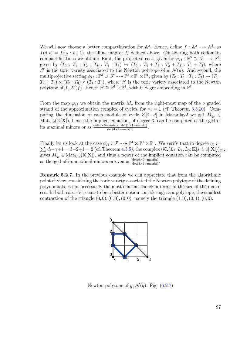
We will now choose a better compactification for A2. Hence, define f : A2 99K A3, asf(s, t) = fI(s : t : 1), the affine map of fI defined above. Considering both codomaincompactifications we obtain: First, the projective case, given by ϕII : P5 ⊃ T 99K P3,given by (T0 : T1 : T2 : T3 : T4 : T5) 7→ (T0 : T4 + T5 : T2 + T3 : T1 + T2), whereT is the toric variety associated to the Newton polytope of g, N (g). And second, themultiprojective setting φII : P3 ⊃ T 99K P1×P1×P1, given by (T0 : T1 : T2 : T3) 7→ (T1 :T2 + T3) × (T2 : T0) × (T1 : T0), where T is the toric variety associated to the Newtonpolytope of f , N (f). Hence T ∼= P1 × P1, with it Segre embedding in P3.

From the map ϕII we obtain the matrix Mν from the right-most map of the ν gradedstrand of the approximation complex of cycles, for ν0 = 1 (cf. Theorem 3.3.10). Com-puting the dimension of each module of cycle Zi[i · d] in Macaulay2 we get Mη0 ∈Mat6,10(K[X]), hence the implicit equation, of degree 3, can be computed as the gcd of

its maximal minors or as det(6×6−matrix). det(1×1−matrix)det(4×4−matrix)

.

Finally let us look at the case φII : T 99K P1 × P1 × P1. We verify that in degree η0 :=∑i di−γ+1 = 3−2+1 = 2 (cf. Theorem 4.3.5), the complex (K•(L1, L2, L3; K[s, t, u][X]))(2,∗)

gives Mη0 ∈ Mat9,12(K[X]), and thus a power of the implicit equation can be computed

as the gcd of its maximal minors or even as det(9×9−matrix)det(3×3−matrix)

.

Remark 5.2.7. In the previous example we can appreciate that from the algorithmicpoint of view, considering the toric variety associated the Newton polytope of the definingpolynomials, is not necessarily the most efficient choice in terms of the size of the matri-ces. In both cases, it seems to be a better option considering, as a polytope, the smallestcontraction of the triangle (3, 0), (0, 3), (0, 0), namely the triangle (1, 0), (0, 1), (0, 0).

Newton polytope of g, N (g). Fig. (5.2.7)

97

Newton polytope of f , N (f). Fig. (5.2.7)

It is clear that the toric variety it defines is T = P2; hence, the setting we consider isthe map ϕ : P2 99K P3 in the projective case, and φI : P2 99K (P1)3 in the multiprojectiveone.

5.3 Applications to the computation of sparse

discriminants

The computation of sparse discriminants is equivalent to the implicitization problem fora parametric variety, to which we can apply the techniques developed in the previoussections. In the situation described in [CD07], a rational map f : Cn 99K Cn given byhomogeneous rational functions of total degree zero is associated to an integer matrixB of full rank. This is done in such a way that the corresponding implicit equation isa dehomogenization of a sparse discriminant of generic polynomials with exponents in aGale dual of B.

Suppose for instance that we take the matrix B below:

B =

1 0 0−2 1 0

1 −2 10 1 −20 0 1

.

In this case, as the colums of B generate the affine relations of the lattice points0, 1, 2, 3, 4. The closed image of the parametrization f is a dehomogenization of theclassical discriminant of a generic univariate polynomial of degree 4. Explicitly, fromthe matrix we get the linear forms l1(u, v, w) = u, l2(u, v, w) = −2u + v, l3(u, v, w) =u− 2v+w, l4(u, v, w) = v− 2w, l5(u, v, w) = w (whose coefficients are read in the rowsof B), and the polynomials f0 = l1 · l3, g0 = l22, f1 = l2 · l4, g1 = l23, f2 = l3 · l5, g2 = l24

98

(the exponents of the linear forms are read from the columns of B) . This constructiongives rise to the following rational map:

f : C3 99K C3

(u, v, w) 7→ (u(u−2v+w)(−2u+v)2

, (−2u+v)(v−2w)(u−2v+w)2

, (u−2v+w)w(v−2w)2

).

First, we see that we can get a map from P2C

because of the homogeneity of the polyno-mials. Also, taking common denominator, we can have a map to P3

C, this is:

f : P2C

99K P3C

(u : v : w) 7→ (f0 : f1 : f2 : f3).

where f0 = (−2u+v)2(u−2v+w)2(v−2w)2 is the common denominator, f1 = u(u−2v+w)3(v−2w)2, f2 = (−2u+v)3(v−2w)3 and f3 = (u−2v+w)w(−2u+v)2(u−2v+w)2.

The problem with this way of projectivizing is that, in general, we cannot implementthe theory developed by L. Buse, M. Chardin, and J-P. Jouanolou, because typically thebase locus has unwanted properties, as a consequence of taking common denominatorand because of combinatorial reasons.

As a possible way out, we propose in this work to consider the morphism of projectiveschemes given by:

φ : P2 99K P1 × P1 × P1

(u : v : w) 7→ (f0 : g0)× (f1 : g1)× (f2 : g2).

where f0 = u(u− 2v+w), g0 = (−2u+ v)2, f1 = (−2u+ v)(v− 2w), g1 = (u− 2v+w)2,f2 = (u−2v+w)w g2 = (v−2w)2. For this particular example, we get that there are onlytwo base points giving rise to an extra factor, namely p = (1 : 2 : 3) and q = (3 : 2 : 1).Is easy to see that those points give rise to two linear factors in the equation of theMacRae invariant.

First, we observe that this situation is better, because we are not adding common zeroes.Moreover, if a point (u : v : w) is a base point here, it also is in the two settings above:the affine and the projective case f .

Remember also that in the n = 2 case, the condition required on the Koszul complexassociated to this map for being acyclic is that the variety X, defined as the commonzeroes of all the 6 polynomials, be empty. In general, the conditions we should check arethe ones imposed by the Avramov’s theorem 4.3.4, as was shown in Theorem 4.4.2.

Note also that if we want to state this situation in the language of approximation com-plexes, we need only to replace K• by Z•, because we can assume that fi, gi are regularsequences, due to the fact that gcd(fi, gi) = 1.

99

Remark 5.3.1. For a matrix like the B above, it is clear that the closed subvariety Xis always empty, due to the fact that all maximal minors of B are not zero, and thepolynomials gi’s involve independent conditions. Then, the only common solution tol22 = l23 = l24 = 0 is (u, v, w) = (0, 0, 0), and so X = ∅ in P2. In this case, it is still better(from an algorithmic approach) to compute the discriminant of a generic polynomial ofdegree 4 in a single variable and then dehomogenize, because, in our setting, the numberof variables is bigger than 1. But when the number of monomials of a sparse polynomialin many variables is not big, this Gale dual approach for the computation of sparsediscriminants provides a good alternative.

We will give next an example where we show a more complicated case.

Example 5.3.2. Let C be the matrix given by

C =

1 −7 −6−1 4 3

1 0 40 1 −1−1 2 0

.

As before, denoting by bi the i-th row of C, we get the linear forms li(u, v, w) =〈bi, (u, v, w)〉 , associated to the row vectors bi of B, where 〈, 〉 stands for the inner prod-uct in C3. Then we define the homogeneous polynomials f0 = l1 · l3, g0 = l2 · l5, f1 =l42 · l4 · l

25, g1 = l71, f2 = l32 · l

43, f2 = l61 · l4. And we obtain the following rational map:

φ : P2 99K P1 × P1 × P1

(u : v : w) 7→ (f0 : g0)× (f1 : g1)× (f2 : g2).

It is easy to see that in this case the variety X is not empty, for instance the pointp = (1 : 1 : −1), defined by l1 = l2 = 0 belongs to X.

As was shown by M. A. Cueto and A. Dickenstein in [CD07, Lemma 3.1 and Thm.3.4], we can interpret the discriminant computed from the matrix C in terms of thedehomogenized discriminant associated to any matrix of the form C ·M , where M is asquare invertible matrix with integer coefficients. That is, we are allowed to do operationson the columns of the matrix C, and still be able to compute the desired discriminantin terms of the matrix obtained from C. In [CD07] they give an explicit formula for thispassage.

In this particular case, we can multiply C from the right by a determinant 1 matrix M ,obtaining

C ·M =

1 −7 −6−1 4 3

1 0 40 1 −1−1 2 0

·

1 12 −10 6 −10 5 1

=

1 0 0−1 −3 0

1 −8 30 11 −2−1 0 −1

.

100

Similar to what we have done before, we can see that the closed subvariety X associatedto the rational map that we obtain from the matrix C · M is empty. Observe that#V (I2) is finite due to the fact that l2 = l4 = 0 or l3 = l4 = 0 or l3 = l5 = 0 should hold.Moreover it is easy to verify that all maximal minors are nonzero, and this conditionimplies that any of the previous conditions define a codimension 2 variety, this is, afinite one. With the notation of Chapter 4, a similar procedure works for seeing see thatcodimA(I3) ≥ 2. Finally the first part of Theorem 4.4.2 implies that the Koszul complexK• is acyclic and so we can compute the Macaulay resultant as its determinant.

Moreover, this property over the minors implies that codimA(I(i0)) = 2 > k + 1 = 1 andthat codimA(I(i0) + I(i1)) = 3 > k+ 1 = 2. So, the second part of Theorem 4.4.2 tells usthat the determinant of the Koszul complex K• in degree greater than (2+8+3)−3 = 10determines exactly the implicit equation of the scheme theoretic image of φ. Observethat, as was shown in [CD07, Thm. 2.5], for this map, we have that deg(φ) = 1.

We remark that the process implemented for triangulating the matrix C via M is notalgorithmic for the moment.

101

6 G-graded Castelnuovo Mumford

Regularity

6.1 Introduction.

Castelnuovo-Mumford regularity is a fundamental invariant in commutative algebra andalgebraic geometry. It is a kind of universal bound for important invariants of gradedalgebras such as the maximum degree of the syzygies and the maximum non-vanishingdegree of the local cohomology modules.

Intuitively, it measures the complexity of a module or sheaf. The regularity of a moduleapproximates the largest degree of the minimal generators and the regularity of a sheafestimates the smallest twist for which the sheaf is generated by its global sections. Ithas been used as a measure for the complexity of computational problems in algebraicgeometry and commutative algebra (see for example [EG84] or [BM93]).

One has often tried to find upper bounds for the Castelnuovo-Mumford regularity interms of simpler invariants. The simplest invariants which reflect the complexity ofa graded algebra are the dimension and the multiplicity. However, the Castelnuovo-Mumford regularity can not be bounded in terms of the multiplicity and the dimension.

Although the precise definition may seem rather technical. Indeed, the two most popu-lar definitions of Castelnuovo-Mumford regularity are the one in terms of graded Bettinumbers and the one using local cohomology.

For the first one, let k be a field, and let I be an homogeneous ideal in a polynomialring R = k[x0, ..., xn] over a field k with characteristic zero. Consider the minimal freeresolution of R/I as a graded R-module,

· · · →⊕

j

R(−di,j)→ · · · →⊕

j

R(−d1,j)→ R→ R/I → 0.

Then, the Castelnuovo-Mumford regularity of R/I is defined as

reg(R/I) = maxi,jdi,j − i.

103

In general, for an R-module M , write Fi =⊕

j R(−di,j) =⊕

j R[−j]βij , for the freeresolution of M . Denote p := pd(M) = n − depth(M). Observe that the maps ofF• ⊗R k are zero, thus, TorRi (M,k) = Hi(F• ⊗R k) = Fi ⊗R k and therefore βij =dimk(TorRi (M,k)j). If TorRi (M,k) 6= 0, set

bi(M) := maxµ : TorRi (M,k)µ 6= 0,

else, bi(M) := −1. By definition, bi(M) is the maximal degree of a minimal generatorof Fi, and therefore of the module of i-th syzygies of M . The Castelnuovo-Mumfordregularity is also a measure of the maximal degrees of generators of the modules Fi:

reg(M) := maxibi(M)− i.

Second, we can give two fundamental results that motivated defining Castelnuovo-Mumford regularity in terms of local cohomology: Grothendieck’s theorem that assertsthat H i

m(M) = 0 for i > dim(M) and i < depth(M), as well as the non vanishing of thesemodules for i = dim(M) and i = depth(M); and Serre’s vanishing theorem that impliesthe vanishing of graded pieces H i

m(M)µ for any i, and µ≫ 0. The Castelnuovo-Mumfordregularity is a measure of this vanishing degree.

If H im(M) 6= 0, set

ai(M) := maxµ|H im(M)µ 6= 0,

else, set ai(M) := −1. Then,

reg(M) := maxiai(M) + i.

The maximum over the positive i’s is also an interesting invariant:

greg(M) := maxi>0ai(M) + i = reg(M/H0

m(M)).

Thus, Castelnuovo-Mumford regularity measures more than the complexity of the idealI and its syzygies. For more discussion on the regularity, refer to the survey of Bayerand Mumford [BM93] or ??.

An interesting question is if one can give bounds for the regularity in terms of the degreesof generators of I. It turns out that such bounds are very sensitive to the singularities ofthe projective scheme defined by I, and in general, are very hard to compute. Its valuein bounding the degree of syzygies and constructing Hilbert schemes has established thatregularity is an indispensable tool in both fields.

The aim of this paper is to develop a multigraded variant of Castelnuovo-Mumfordregularity in the spirit of [MS04] and [HW04]. We work with modules over a commutativering R graded by a finitely generated abelian group G.

104

One motivation for studying regularity over multigraded polynomial rings comes fromtoric geometry. For a simplicial toric variety X, the homogeneous coordinate ring, in-troduced in [Cox95], is a polynomial ring S graded by the divisor class group G of X.The dictionary linking the geometry of X with the theory of G-graded S-modules leadsto geometric interpretations and applications for multigraded regularity.

In [HW04] Hoffman and Wang define the concept of regularity for bigraded modules overa bigraded polynomial ring motivated by the geometry of P1 × P1. They prove analogsof some of the classical results on m-regularity for graded modules over polynomialalgebras.

In [MS04] Maclagan and Smith develop a multigraded variant of Castelnuovo-Mumfordregularity also motivated by toric geometry. They work with modules over a polynomialring graded by a finitely generated abelian group, in order to establish the connectionwith the minimal generators of a module and its behavior in exact sequences. In thischapter, we extend this work restatings some of the results in [MS04].

As in the standard graded case, our definition of multigraded regularity involves thevanishing of graded components of local cohomology, following [HW04].

Our notion of Multigraded Castelnuovo-Mumford regularity follows of existing ideas of[HW04] and [MS04]. In the standard graded case, it reduces to Castelnuovo-Mumfordregularity (cf. [BM93]). When S is the homogeneous coordinate ring of a product ofprojective spaces, multigraded regularity is the weak form of bigraded regularity definedin [HW04].

One point we are interestied in remark is that Castelnuovo-Mumford regularity establisha relation between the degrees of vanishing of local cohomology modules and the degreeswhere Tor modules vanish. This provides a powerfull tool for computing one region ofZ in terms of the other.

In this chapter, we deal with G-graded polynomial rings, where G is any abelian groupof finite rank. We exploit some of the simililaties we get in multigraded regularity withstandard regularity, being able to compute the regions of G where local cohomologymodules vanish in terms of the supports of Tor modules, and viceversa.

Indeed, for S be a commutative ring, G an abelian group and R := S[X1, . . . , Xn], withdeg(Xi) = γi and deg(s) = 0 for s ∈ S, setting B ⊆ (X1, . . . , Xn) a graded R-ideal andC be the monoid generated by γ1, . . . , γn, we propose in Definition 6.3.1 that:

For γ ∈ G, and for a graded R-module M is weakly γ-regular if

γ 6∈⋃

i

SuppG(H iB(M)) + Ei.

105

We also set that if further, M is weakly γ′-regular for any γ′ ∈ γ+C, then M is γ-regular

and

reg(M) := γ ∈ G | M is γ−regular.

We deduce from the definition that reg(M) is the maximal set S of elements in G suchthat S + C = S and M is γ-regular for any γ ∈ S, and allows generalizing the classicalfact that weak regularity implies regularity.

Precisely, we prove in Theorem 6.3.3, for a G-graded R-module M , that for all j ≥ 0,

⋂

γ∈Ej

(reg(M) + γ)⋂

SuppG(TorRj (M,S)) = ∅.

This result generalizes the fact that when G = Z and the grading is standard, reg(M)+j ≥ end(TorRj (M,S)).

6.2 Local Cohomology and graded Betti numbers

In this chapter we develop a regularity theory for graded rings. Our aim is to give a moregeneral setting to that in [MS04] and [HW04], and to establish a clear relation betweensupports of local cohomology modules with Tor modules and Betti numbers.

Throughout this chapter let G be a finitely generated abelian group, and let R be acommutative G-graded ring with unit. Let B be a homogeneous ideal of R.

Remark 6.2.1. Is of particular interest the case where R is a polynomial ring in nvariables and G = Zn/K, is a quotient of Zn by some subgroup K. Note that, if M is aZn-graded module over a Zn-graded ring, and G = Zn/K, we can give to M a G-gradingcoarser than its Zn-grading. For this, define the G-grading on M by setting, for eachγ ∈ G, Mγ :=

⊕d∈π−1(γ)Md.

In order to fix the notation, we state the following definitions concerning local coho-mology of graded modules, and support of a graded modules M on G. Recall that thecohomological dimension cdB(M) of a module M is −∞ if M = 0 and maxi ∈ Z :H iB(M) = 0 otherwise.

Definition 6.2.2. Let M be a graded R-module, the support of the module M isSuppG(M) := γ ∈ G : Mγ 6= 0.

106

Observe that if F• is a free resolution of a graded module M , much information on themodule can be read from the one of the resolution. Next we present a result that permitsdescribing the support of a graded module M in terms of some homological informationof a complex which need not be a resolution of M , but M is its first non-vanishinghomology.

Definition 6.2.3. For all i, j ∈ Z we define a condition (Dij) as above

H iB(Hj(C•)) 6= 0 implies H i+ℓ+1

B (Hj+ℓ(C•)) = H i−ℓ−1B (Hj−ℓ(C•)) = 0 for all ℓ ≥ 1.

(Dij)

We have the following result on the support of the local cohomology modules of thehomologies of C•.

Theorem 6.2.4. Let C• be a complex of graded R-modules and i ∈ Z. If (Dij) holds,then

SuppG(H iB(Hj(C•))) ⊂

⋃

k∈Z

SuppG(H i+kB (Cj+k)).

Proof. Consider the two spectral sequences that arise from the double complex C•BC• ofgraded R-modules.

The first spectral sequence has as second screen ′2E

ij = H i

B(Hj(C•)). Condition (Dij)implies that ′

∞Eij = ′

2Eij = H i

B(Hj(C•)). The second spectral sequence has as first screen′′1E

ij = H i

B(Cj).

By comparing both spectral sequences, we deduce that, for γ ∈ G, the vanishing of(H i+k

B (Cj+k))γ for all k implies the vanishing of (′∞Ei+ℓj+ℓ)γ for all ℓ, hence the one of

(H iB(Hj(C•)))γ.

Remark 6.2.5. Let C• be a complex of graded R-modules. Consider the followingconditions

1. C• is a right-bounded complex, say Cj = 0 for j < 0 and, cdB(Hj(C•)) ≤ 1 for allj 6= 0.

2. For some q ∈ Z ∪ −∞, Hj(C•) = 0 for all j < q and, cdB(Hj(C•)) ≤ 1 for allj > q.

3. Hj(C•) = 0 for j < 0 and cdB(Hk(C•)) ≤ k + i for all k ≥ 1.

Then,

(i) (1)⇒ (2)⇒ (Dij) for all i, j ∈ Z, and

(ii) (3)⇒(Dij) for j = 0.

107

Proof. For proving item (i), it suffices to show that (2) ⇒ (Dij) for all i, j ∈ Z since(1)⇒ (2) is clear.

Let ℓ ≥ 1.

Condition (2) implies that H iB(Hj(C•)) = 0 for j > q and i 6= 0, 1 and for j < q. If

H iB(Hj(C•)) 6= 0, either j > q and i ∈ 0, 1 in which case j + ℓ > q and i + ℓ + 1 ≥ 2

and i− ℓ− 1 < 0, or j = q in which case j + ℓ > q and i + ℓ + 1 ≥ 2 and j − ℓ < 0. Inboth cases the asserted vanishing holds.

Condition (3) implies that H i+ℓ+1B (Hℓ(C•)) = 0 and Hj−ℓ(C•) = 0.

6.2.1 From Local Cohomology to Betti numbers

Assume R := S[X1, . . . , Xn] is a polynomial ring over a commutative ring S, B ⊆(X1, . . . , Xn), deg(Xi) = γi ∈ G for 1 ≤ i ≤ n and deg(s) = 0 for s ∈ S. Setγ := (γ1, . . . , γn) ∈ Gn.

Definition 6.2.6. Set E0 := 0 and El := γi1 + · · ·+ γil : i1 < · · · < il for l 6= 0.

Observe that if l < 0 or l > n, then El = ∅. If γi = γ for all i, El = l · γ when El 6= ∅.

Remark 6.2.7. For an R-module M , we denote by M [γ′] the shifted module by γ′ ∈ G,with M [γ′]γ := Mγ′+γ for all γ ∈ G.

Let M be a graded R-module. Write KM• := K•(X1, . . . , Xn;M) for the Koszul complexof the sequence (X1, . . . , Xn) with coefficients in M . We next establish a relationshipbetween the support of the local cohomologies of its homologies and graded Betti numbersof M .

The Koszul complex KM• is graded with KMl :=

⊕i1<···<il

M [−γi1 − · · · − γil ]. Let ZMi

and BMi be the Koszul i-th cycles and boundaries modules, with the grading that makes

the inclusions ZMi , B

Mi ⊂ KM

i a map of degree 0 ∈ G, and set HMi = ZM

i /BMi .

Theorem 6.2.8. Let M be a G-graded R-module. Then

SuppG(TorRj (M,S)) ⊂⋃

k≥0

(SuppG(HkB(M)) + Ej+k),

for all j ≥ 0.

108

Proof. Notice that HMj ≃ TorRj (M,S) is annihilated by B, hence has cohomological

dimension 0 relatively to B. According to Remark 6.2.5 (case (1)), Theorem 6.2.4 appliesand shows that

SuppG(TorRj (M,S)) ⊂⋃

ℓ≥0

SuppG(HℓB(Kj+ℓ)) =

⋃

k≥0

(SuppG(HkB(M)) + Ej+k).

6.2.2 From Betti numbers to Local Cohomology

We keep hypotheses as in section 6.2.1

Theorem 6.2.9. Let M be a graded R-module and F• be a graded complex of free R-modules, with H0(F•) = M . Write Fi =

⊕j∈Ei

R[−γij] and Ti := γij | j ∈ Ei. Letℓ ≥ 0 and assume cdB(Hj(F•)) ≤ ℓ+ j for all j ≥ 1. Then,

SuppG(HℓB(M)) ⊂

⋃

i≥0

(SuppG(Hℓ+iB (R)) + Ti).

Proof. Remark 6.2.5 (case (3)) shows that Theorem 6.2.4 applies for estimating thesupport of local cohomologies of H0(F•), and provides the quoted result as

SuppG(HpB(R[−γ])) = SuppG(Hp

B(R)) + γ, and SuppG(⊕i∈ENi) = ∪i∈ESuppG(Ni)

for any set of graded modules Ni, i ∈ E.

Corollary 6.2.10. Assume that S is a field and let M be a graded R-module. Then, forany ℓ,

SuppG(HℓB(M)) ⊂

⋃

i≥0

(SuppG(Hℓ+iB (R)) + SuppG(TorRi (M,S))).

If (S,m, k) is local, the spectral sequence TorSp (TorRq (M,S), k) ⇒ TorRp+q(M,k) showsthat

SuppG(TorRi (M,k)) ⊆⋃

j≤i

SuppG(TorRj (M,S))

as S ⊂ R0. It implies the following:

Corollary 6.2.11. Assume that (S,m, k) is local and let M be a graded R-module. Then,for any ℓ,

SuppG(HℓB(M)) ⊂

⋃i≥0(SuppG(Hℓ+i

B (R)) + SuppG(TorRi (M,k)))

⊂⋃i≥j≥0(SuppG(Hℓ+i

B (R)) + SuppG(TorRj (M,S))).

109

Which in turn shows that :

Corollary 6.2.12. Let M be a graded R-module. Then, for any ℓ,

SuppG(HℓB(M)) ⊂

⋃

i≥j≥0

(SuppG(Hℓ+iB (R)) + SuppG(TorRj (M,S))).

Proof. Let γ ∈ SuppG(HℓB(M)). Then Hℓ

B(M)γ 6= 0, hence there exists p ∈ Spec(S)such that (Hℓ

B(M)γ) ⊗S Sp = HℓB⊗SSp

(M ⊗S Sp) 6= 0. Applying Corollary 6.2.11 theresult follows since both the local cohomology functor and the Tor functor commutewith localization in S, and preserves grading as S ⊂ R0.

6.3 Castelnuovo-Mumford regularity

We have mentionned in the beginning of this chapter that one point we are interestiedin remark is that Castelnuovo-Mumford regularity establishes a relation between thedegrees of vanishing of local cohomology modules and the degrees where Tor modulesvanish. It is clear that this provides a powerfull tool for computing one region of Z interms of the other.

As we have promissed, in this section we give a definiton for a G-graded R-module Mand γ ∈ G to be weakly γ-regular or just γ-regular, depending if γ is or is not on theshifted suport of some local cohomology modules of M (cf. 6.3.1). This definition allowsus to generalize the classical fact that weak regularity implies regularity.

In the later part of this section, in Theorem 6.3.3, we prove that for j ≥ 0, the supportsof TorRj (M,S) does not meet the support of any shifted regularity region reg(M) + γfor γ moving on Ej. As we have mentioned in the introduction of this chapter, thisresult generalizes the fact that when G = Z and the grading is standard, reg(M) + j ≥end(TorRj (M,S)).

6.3.1 Regularity for Local Cohomology modules

Let S be a commutative ring, G an abelian group and R := S[X1, . . . , Xn], withdeg(Xi) = γi and deg(s) = 0 for s ∈ S. Let B ⊆ (X1, . . . , Xn) be a graded R-idealand C be the monoid generated by γ1, . . . , γn.

110

Definition 6.3.1. For γ ∈ G, a graded R-module M is weakly γ-regular if

γ 6∈⋃

i

SuppG(H iB(M)) + Ei.

If further M is weakly γ′-regular for any γ′ ∈ γ + C, then M is γ-regular and

reg(M) := γ ∈ G | M is γ−regular.

It immediately follows from the definition that reg(M) is the maximal set S of elementsin G such that S + C = S and M is γ-regular for any γ ∈ S.

Let γ1, . . . , γn = µ1, . . . , µp, with µi 6= µj for i 6= j. Denote by pi the ideal generatedby the variables of degree µi.

The following lemma generalizes the classical fact that weak regularity implies regularityunder some extra requirement.

Lemma 6.3.2. Assume that B ⊂ pi for every i. Let M be a graded R-module. If M isweakly γ-regular and either H0

B(M)γ+C = 0 or M is generated by elements whose degreesdo not belong to γ + C, then M is γ-regular.

Proof. We induct on w(M) := n−m, where m is the number of variables acting as 0 onM .

Let i ∈ 1, . . . , p. We have to show that M is weakly (γ + µi)-regular if one of the twoconditions of the Lemma is satisfied. Assume that the variables Xj for j = j0i, . . . , jtiare the ones of degree µi.

If w(M) = 0, then M = 0 :M B = H0B(M). Further if M = H0

B(M), both requirementsare equivalent and the result follows as H i

B(M) = 0 for i > 0.

Our statement is unchanged by faithfully flat extension and the Dedekind-MertensLemma shows that after making a polynomial extension S ′ := S[U1, . . . Ut] of S, theelement fi := Xj0i

+ U1Xj1i+ · · ·+ UtXjti is a non-zero divisor on M/H0

pi(M), hence on

M ′ := M/H0B(M), as B ⊂ pi by hypothesis.

Notice that w(M/fiM) < w(M) after identifyingR/(fi) withR′ := S ′[X1, . . . , Xj0i, . . . , Xn].

For any ℓ, the exact sequence 0 → (0 :M (fi)) → M → M(µi) → (M/fiM)(µi) → 0gives rise to an exact sequence

HℓB(M)→ Hℓ

B(M)(µi)→ HℓB(M/fiM)(µi)→ Hℓ+1

B (M).

The right part of the sequence shows that M/fiM is weakly γ-regular, hence, by in-duction hypothesis, γ-regular if M/fiM is generated by elements whose degrees do not

111

belong to γ + C (for instance if M is so) and (M/fiM)/H0B(M/fiM) is γ-regular in any

case.

From the left part of the sequence, we deduce that M is (γ+µi)-regular if M is generatedby elements whose degrees do not belong to γ + C and M/H0

B(M) is (γ + µi)-regular inany case, which proves our claim.

Theorem 6.3.3. Let M be a G-graded R-module. Then

⋂

γ∈Ej

(reg(M) + γ)⋂

SuppG(TorRj (M,S)) = ∅

for all j ≥ 0.

When G = Z and the grading is standard, this reads with the usual definition ofreg(M) ∈ Z:

reg(M) + j ≥ end(TorRj (M,S)).

Proof. If γ ∈ SuppG(TorRj (M,S)), then it follows from Theorem 6.3.3 that γ ∈ SuppG(HℓB(M))+

Ej+ℓ for some ℓ. Hence

γ − γi1 − · · · − γij+ℓ∈ SuppG(Hℓ

B(M))

for some i1 < · · · < ij+ℓ. By definition it follows that if µ ∈ reg(M) and t1 < · · · < tℓ,then

γ − γi1 − · · · − γij+ℓ6= µ− γt1 − · · · − γtℓ

in particular choosing tk := ij+k one has

γ − γi1 − · · · − γij 6∈ reg(M).

On the other hand, Corollary 6.2.12 shows that :

Proposition 6.3.4. Let M be a G-graded R-module and set Ti := SuppG(TorRi (M,S)).Then, for any ℓ,

SuppG(HℓB(M) + Eℓ) ⊂

⋃

i≥j

(SuppG(Hℓ+iB (R)) + Eℓ + Tj).

If further S is a field,

SuppG(HℓB(M) + Eℓ) ⊂

⋃

i

(SuppG(Hℓ+iB (R)) + Eℓ + Ti).

112

In some applications it is useful to consider local cohomologies of indices at least equalto some number, for instance positive values or values at least two. In view of Lemma6.3.2, most of the time weak regularity and regularity agrees in this case. We set :

regℓ(M) := γ | ∀γ′ ∈ C, γ + γ′ 6∈⋃

i≥ℓ

SuppG(H iB(M)) + Ei.

With this notation, Proposition 6.3.4 implies the following

Theorem 6.3.5. Let M be a G-graded R-module and set Ti := SuppG(TorRi (M,S)).Then, for any ℓ,

regℓ(M) ⊇⋂

j≤i,γ∈Tj ,γ′∈Ei

regℓ+i(R) + γ − γ′ ⊇ regℓ(R) +⋂

j≤i,γ∈Tj ,γ′∈Ei

γ − γ′ + C.

The above intersection can be restricted to i ≤ cdB(R)− ℓ. If further S is a field,

regℓ(M) ⊇⋂

i,γ∈Ti,γ′∈Ei

regℓ+i(R) + γ − γ′ ⊇ regℓ(R) +⋂

i,γ∈Ti,γ′∈Ei

γ − γ′ + C.

When G = Z and the grading is standard, this reads with the usual definition ofregℓ(M) ∈ Z:

regℓ(M) ≤ regℓ(R) + maxiend(TorRi (M,S))− i.

Proof. If µ 6∈ regℓ(M), by Proposition 6.3.4, there exists i ≥ j such that

µ ∈ SuppG(Hℓ+iB (R)) + Eℓ + Tj

hence there exists γ′ ∈ Ei and γ ∈ Tj such that

µ+ γ′ − γ ∈ SuppG(Hℓ+iB (R)) + Ei+ℓ.

Therefore µ 6∈ regℓ+i(R) + γ − γ′.

6.4 Multigraded polynomial rings

6.4.1 Local cohomology of multigraded polynomial rings

Throughout this section, we will adopt the following convention: Let s and m be fixedpositive integers, r1 ≤ · · · ≤ rs non-negative integers, and write xi = (xi,1, . . . , xi,ri)for 1 ≤ i ≤ s. Define Ri := k[xi] the Z-graded polynomial ring in the variables xifor 1 ≤ i ≤ s, R =

⊗k Ri, and R(a1,...,as) :=

⊗k(Ri)ai

stands for its bigraded partof multidegree (a1, . . . , as). Let f1, . . . , fm ∈ R be multihomogeneous polynomials ofmultidegree di on xi, and denote f := (f1, . . . , fm).

113

Definition 6.4.1. We define Ri := 1xi,1···xi,ri

k[x−1i,1 , . . . , x

−1i,ri

]. Given integers 1 ≤ i1 <

· · · < it ≤ s, take α = i1, . . . , it, and set Rα :=(⊗

j∈α Rj

)⊗k(⊗

j /∈αRj

).

Remark 6.4.2. Observe that Ri∼= Ri ⊗k

⊗j 6=iRj.

Definition 6.4.3. Given integers 1 ≤ i1 < · · · < it ≤ s, take α = i1, . . . , it. For anyinteger j write sg(j) := 1 if j ∈ α and sg(j) := 0 if j /∈ α. We define

Qα :=∏

1≤j≤s

(−1)sg(j)N− sg(j)rjej ⊂ Zs,

the shift of the orthant whose coordinates i1, . . . , it are negative and the rest are allpossitive. We denote aα := ai1 + · · ·+ ait and |α| = ri1 + · · ·+ rit .

Lemma 6.4.4. For every α ⊂ 1, . . . , s, we have SuppZs(Rα) = Qα.

Remark 6.4.5. For α, β ⊂ 1, . . . , s, if α 6= β, then Qα ∩Qβ = ∅.

Lemma 6.4.6. Given integers 1 ≤ i1 < · · · < it ≤ s, take α = i1, . . . , it, there aregraded isomorphisms or R-modules

H |α|aα

(R) ∼= Rα. (6.1)

Proof. Recall that for any ring S and any S-module M , if x1, . . . , xn are variables, then

H i(x1,...,xn)(M [x1, . . . , xn]) =

0 if i 6= n

1x1···xn

M [x−11 , . . . , x−1

n ] for i = n.(6.2)

We induct on |α|. The result is obvious for |α| = 1. Assume that |α| ≥ 2 and (6.1)holds for |α| − 1. Take I = ai1 · · · ait−1 and J = ait . There is an spectral sequenceHpJ(H

qI (R))⇒ Hp+q

I+J(R). By (6.2), HpJ(R) = 0 for p 6= rit . Hence, the spectral sequence

stabilizes in degree 2, and gives HritJ (H

|α|−ritI (R)) ∼= H

|α|I+J(R). The result follows by

applying (6.2) with M = H|α|−ritI (R), and inductive hypothesis.

Lemma 6.4.7. We have

HℓB(R) ∼=

⊕

1 ≤ i1 < · · · < it ≤ sri1 + · · · + rit

− (t− 1) = ℓ

Hri1+···+ritai1

+···+ait(R) ∼=

⊕

α ⊂ 1, . . . , s|α| − (#α− 1) = ℓ

Rα. (6.3)

Proof. The second isomorphism follows from 6.4.6. For proving the first isomorphism,we induct on s. The result is obvious for s = 1. Assume that s ≥ 2 and (6.3) holds for

114

s− 1. Take I = a1 · · · as−1 and J = as. The Mayer-Vietoris long exact sequence of localcohomology for I and J is

· · · → HℓI+J(R)

ψℓ→ HℓI(R)⊕Hℓ

J(R)→ HℓIJ(R)→ Hℓ+1

I+J(R)ψℓ+1→ Hℓ+1

I (R)⊕Hℓ+1J (R)→ · · · .

(6.4)Remark that if ℓ < rs, then Hℓ

J(R) = HℓI+J(R) = Hℓ+1

I+J(R) = 0. Hence, HℓB(R) ∼= Hℓ

I(R).

Write R := R1 ⊗k · · · ⊗k Rs−1. Since the variables xs does not appear on I, by flatnessof Rs and the last isomorphism, we have that Hℓ

B(R) ∼= HℓB(R)⊗k Rs. In this case, the

result follows by induction.

Thus, assume ℓ ≥ rs. We next show that the map ψℓ in the sequence (6.4) is the zeromap for all ℓ. Indeed, there is an spectral sequence Hp

J(HqI (R)) ⇒ Hp+q

I+J(R). Since

HpJ(R) = 0 for p 6= rs, it stabilizes in degree 2, and gives Hrs

J (Hℓ−rsI (R)) ∼= Hℓ

I+J(R). Wehave graded isomorphisms

HrsJ (Hℓ−rs

I (R)) ∼= HrsJ (Hℓ−rs

I (R)⊗k Rs) ∼= (Hℓ−rsI (R))[x−1

s ] ∼= Hℓ−rsI (R)⊗k Rs, (6.5)

where the first isomorphism comes from flatness of Rs over k, the second isomorphismfollows from equation (6.2) taking M = Hℓ−rs

I (R). By (6.5) and the inductive hypothesiswe have that.

HrsJ (Hℓ−rs

I (R)) ∼=⊕

1 ≤ i1 < · · · < it−1 ≤ s− 1ri1 + · · · + rit−1

− (t− 2) = ℓ− rs

Hri1+···+rit−1

ai1+···+ait−1

(R)⊗k Rs. (6.6)

Now, observe that the map (Hℓ−rsI (R))[x−1

s ]→ HℓI(R)⊕Hℓ

J(R) is graded of degree 0. Re-call from Lemma 6.4.4 and 6.4.6, and Remark 6.4.5 we deduce SuppZs((Hℓ−rs

I (R))[x−1s ])∩

SuppZs(HℓI(R) ⊕Hℓ

J(R)) = ∅. Thus, every homogeneous element on (Hℓ−rsI (R))[x−1

s ] isnecessary mapped to 0.

Hence, for each ℓ, we have a short exact sequence

0→ HℓI(R)⊕Hℓ

J(R)→ HℓIJ(R)→ Hrs

J (Hℓ+1−rsI (R))→ 0. (6.7)

Observe that this sequence has maps of degree 0, and for each degree a ∈ Zs the homo-geneous strand of degree a splits. Moreover,

SuppZs((Hℓ+1−rsI (R))[x−1

s ]) ⊔ SuppZs(HℓI(R)⊕Hℓ

J(R)) = SuppZs(HℓIJ(R)).

Namely, every monomial in HℓIJ(R) eather comes from the module (Hℓ+1−rs

I (R))[x−1s ] or

it is mapped to HℓI(R) ⊕ Hℓ

J(R) injectively, splitting the sequence (6.7) of R-modules.Hence,

HℓB(R) ∼= Hℓ

I(R)⊕HℓJ(R)⊕Hrs

J (Hℓ+1−rsI (R)).

Now, HℓI(R) ∼= Hℓ

B(R)⊗k Rs, HℓJ(R) = 0 if ℓ 6= rs and Hrs

J (R) = Rs. The result followsby induction and equation (6.6).

115

Corollary 6.4.8. Let M be a graded R-module. Then, for any ℓ,

SuppG(HℓB(M)) ⊂

⋃i≥0

(SuppG(Hℓ+iB (R)) + SuppG(TorRi (M,k)))

=⋃i≥0

⋃

1 ≤ i1 < · · · < it ≤ s

ri1+ · · · + rit

− (t − 1) = ℓ + i

Qi1,...,it + SuppG(TorRi (M,k))

.

Proof. Follows from Corollary 6.2.10 and Lemma 6.4.7.

Recall that we have seen in Theorem 6.2.4 that if C• is a complex of graded R-modules,assuming (Dij) we have that for all i ∈ Z

SuppG(H iB(Hj(C•))) ⊂

⋃

k∈Z

SuppG(H i+kB (Cj+k)).

For i = 1, . . . ,m, take fi ∈ R homogeneous of the same degree γ for all i. Let M bea graded R-module. Denote by KM• the Koszul complex K•(f1, . . . , fm;R) ⊗R M . TheKoszul complex KM• is graded with Ki :=

⊕l0<···<li

R(−i · γ). Set HMi := Hi(K

M• ) the

i-th homology module of KM• .

Corollary 6.4.9. If cdB(HMi ) ≤ 1 for all i > 0. Then, for all j ≥ 0

SuppG(H iB(HM

j )) ⊂⋃

k∈Z

(SuppG(HkB(M)) + k · γ) + (j − i) · γ.

Proof. This follows by a change of variables in the index k in Lemma 6.2.4. Since C• isKM• and KM

i :=⊕

l0<···<liM(−i · γ), we get that

SuppG(H iB(HM

j )) ⊂⋃

k∈Z

SuppG(HkB(KM

k+j−i)) =⋃

k∈Z

(SuppG(HkB(M)[−(k + j − i) · γ]).

The conclusion follows from Remark 6.2.7.

Remark 6.4.10. In the special case where M = R, we deduce that if cdB(Hi) ≤ 1 forall i > 0,

SuppG(H iB(Hj)) ⊂

⋃

k∈Z

(SuppG(HkB(R)) + k · γ) + (j − i) · γ, for all i, j.

Take j = 0 and write I := (f1, . . . , fm), we get

SuppG(H iB(R/I)) ⊂

⋃

k∈Z

(SuppG(HkB(R)) + (k − i) · γ), for all i.

116

Example 6.4.11. Let k be a field. Take R1 := k[x1, x2], R2 := k[y1, y2, y3, y4], andG := Z2. Write R := R1⊗kR2 and set deg(xi) = (1, 0) and deg(yi) = (0, 1) for all i. Seta1 := (x1, x2), a2 := (y1, y2, y3, y4) and define B := a1 · a2 ⊂ R the irrelevant ideal of R,and m := a1 + a2 ⊂ R, the ideal corresponding to the origin in Spec(R).

From Lemma 6.4.7, it follows that

1. H2B(R) ∼= R1

∼= H2a1

(R) = ω∨R1⊗k R2,

2. H4B(R) ∼= R2

∼= H4a2

(R) = R1 ⊗k ω∨R2

,

3. H5B(R) ∼= R1,2

∼= H6m(R) = ω∨

R,

4. HℓB(R) = 0 for all ℓ 6= 2, 4 and 5.

Hence, we see that

1. SuppG(H2B(R)) = SuppG(R1) = Q1 = −N× N + (−2, 0), .

2. SuppG(H4B(R)) = SuppG(R2) = Q2 = N×−N + (0,−4), .

3. SuppG(H5B(R)) = SuppG(R1,2) = Q1,2 = −N×−N + (−2,−4), .

b

b

b

bbb

(0,0)

(-1,-3)

(-2,0)

(-2,-4) (0,-4)

SuppZ2(H2

B(R))

SuppZ2(H5

B(R)) SuppZ2(H4

B(R))

Take f1, . . . , fm homogeneous elements of bidegree γ, and write I := (f1, . . . , fm). As-sume cdB(R/I) ≤ 1, hence cdB(Hi) ≤ 1 for all i. We will compute reg(R/I).

Define for every γ ∈ G,

SB(γ) :=⋃

k≥0

(SuppG(HkB(R)) + k · γ). (6.8)

117

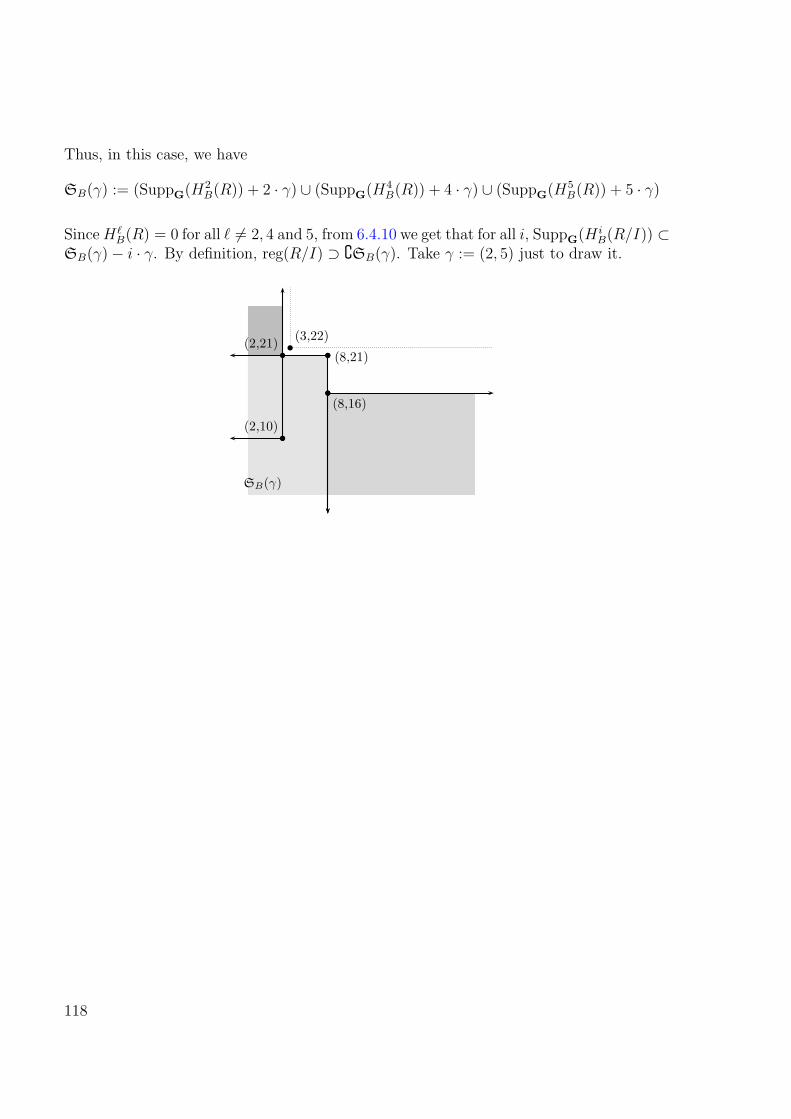
Thus, in this case, we have

SB(γ) := (SuppG(H2B(R)) + 2 · γ) ∪ (SuppG(H4

B(R)) + 4 · γ) ∪ (SuppG(H5B(R)) + 5 · γ)

SinceHℓB(R) = 0 for all ℓ 6= 2, 4 and 5, from 6.4.10 we get that for all i, SuppG(H i

B(R/I)) ⊂SB(γ)− i · γ. By definition, reg(R/I) ⊃ ∁SB(γ). Take γ := (2, 5) just to draw it.

bb

bb

bb

(2,10)

(8,16)

(8,21)(2,21)

SB(γ)

(3,22)

118

7 Implicit equation of multigraded

hypersurfaces

7.1 Introduction

In this chapter we present a method for computing the implicit equation of a hypersurfacegiven as the image of a rational map φ : X 99K Pn, where X is an arithmetically Cohen-Macaulay toric variety. In Chapters 3 and 4, the approach consisted in embedding thespace X in a projective space, via a toric embedding. The need of the embedding comesfrom the necessity of a Z-grading in the coordinate ring of X , in order to study itsregularity.

The aim of this chapter is to give an alternative to this approach: we study the implici-tization problem directly, without an embedding in a projective space, by means of theresults od Chapter 6. Indeed, we deal with the multihomogeneous structure of the coor-dinate ring S of X , and we adapt the method developed in Chapters 1, 3 and 4 to thissetting. The main motivations for our change of perspective are that it is more naturalto deal with the original grading on X , and that the embedding leads to an artificialhomogenization process that makes the effective computation slower, as the number ofvariables to eliminate increases.

In Definition 7.2.11 we introduce the “good” region in G where the approximation com-plex Z• and the symmetric algebra SymR(I) has no B-torsion. Indeed, we define forγ ∈ G, RB(γ) :=

⋃0<k<minm,cdB(R)(SB(γ) − k · γ) ⊂ G. This goes in the direction

of proving the main theorem of this chapter, Theorem 7.3.4. Precisely, when X is a(d − 1)-dimensional non-degenerate toric variety over a field K, and S its Cox ring (cf.2.4). For a rational map φ : X 99K Pd defined by d+ 1 homogeneous elements of degreeρ ∈ Cl(X ). If dim(V (I)) ≤ 0 in X and V (I) is almost a local complete intersection offV (B), we prove in Therem 7.3.4 that,

det((Z•)γ) = Hdeg(φ) ·G ∈ K[T],

for all γ /∈ RB(ρ), where H stands for the irreducible implicit equation of the image ofφ, and G is relatively prime polynomial in K[T].

This result is a restatement of that in Theorem 4.4.11 and Corollary 3.3.10.

119

7.2 Commutative algebra tools

7.2.1 Regularity for commutative G-graded rings

Throughout this chapter let G be a finitely generated abelian group, and let R be acommutative G-graded ring with unity. Let B be an homogeneous ideal of R. Take ma positive integer and let f := (f0, . . . , fm) be a tuple of homogeneous elements of R,with deg(fi) = γ, and set γ := (γ0, . . . , γm). Write I = (f0, . . . , fm) for the homogeneousR-ideal generated by the fi.

Our main motivation in Chapter 6 for considering regularity in general G-gradings comesfrom toric geometry. Among G-graded rings, homogeneous coordinate rings of a toricvarieties are of particular interest in geometry. When X is a toric variety, G := Cl(T )is the (torus-invariant) divisor class group of X . In this case, the grading can be relatedgeometrically with the action of this group on the toric variety. Thus, as we mentionnedin Remark 6.2.1 is of particular interest the case where R is a polynomial ring in nvariables and G = Zn/K, is a quotient of Zn by some subgroup K. Note that, if M is aZn-graded module over a Zn-graded ring, and G = Zn/K, we can give to M a G-gradingcoarser than its Zn-grading. For this, define the G-grading on M by setting, for eachγ ∈ G, Mγ :=

⊕d∈π−1(γ)Md.

In this section we will present several results concerning vanishing of graded parts ofcertain modules. In our applications we will mainly focus on vanishing of Koszul cyclesand homologies. We recall here what the support of a graded modules M is. Recall fromDefinition 6.2.2 that for graded R-module M , we define the support of the module Mon G as SuppG(M) := γ ∈ G : Mγ 6= 0.

Recall that from Theorem 6.2.4 that for a complex C• of graded R-modules, for whichone of the following holds

1. For some q ∈ Z, Hj(C•) = 0 for all j < q and, cdB(Hj(C•)) ≤ 1 for all j > q.

2. cdB(Hj(C•)) ≤ 1 for all j ∈ Z.

we get that, for i = 0, 1,

SuppG(H iB(Hj(C•))) ⊂

⋃

k∈Z

SuppG(H i+kB (Cj+k)).

We have seen in the Lemma above that much of the information of the supports of thelocal cohomologies of the homologies of a complex C• is obtained from the supports ofthe local cohomologies of the complex. For instance, if C• is a free resolution of a gradedR-module Q, the supports of the local cohomologies of Q can be controlled in terms ofthe supports of the local cohomologies of the base ring R, and the shifts appearing inthe Ci’s.

120

In order to lighten the lecture of this chapter, following equation (6.8), we extend thedefinition as follows

Let P be a graded R-module. For every γ ∈ G, we define

SB(γ;P ) :=⋃

k≥0

(SuppG(HkB(P )) + k · γ). (7.1)

We will write SB(γ) := SB(γ;R) as in equation (6.8).

Remark 7.2.1. Recall from Remark 6.2.7 that for an R-module P , we denote by P [γ′]the shifted module by γ′ ∈ G, with P [γ′]γ := Pγ′+γ. Hence, SB(γ;P [γ′]) = SB(γ;P )−γ′.

We apply Theorem 6.2.4 and Remark 6.2.5 in the particular case where C• is the Koszulcomplex of a tuple f with coefficients in P , and we bound the support of the localcohomologies of its homologies in terms of the sets SB(γ;P ).

Let P be a G-graded R-module. Denote by KP• the Koszul complex K•(f;R) ⊗R P . Ifthe fi are G-homogeneous of the same degree γ for all i, the Koszul complex KP• isG-graded with Ki :=

⊕l0<···<li

R(−i · γ). Let ZPi and BP

i be the Koszul i-th cycles and

boundaries modules, with the grading that makes the inclusions ZPi , B

Pi ⊂ KP

i a map ofdegree 0 ∈ G, and set HP

i = ZPi /B

Pi .

Recall that we have seen in Corollary 6.4.9 that if cdB(HPi ) ≤ 1 for all i > 0, then, for

all j ≥ 0SuppG(H i

B(HPj )) ⊂ SB(γ;P ) + (j − i) · γ.

Recall from Remark 6.4.10 that

Remark 7.2.2. If cdB(Hi) ≤ 1 for all i > 0,

SuppG(H iB(Hj)) ⊂

⋃

k∈Z

(SuppG(HkB(R)) + k · γ) + (j − i) · γ, for all i, j.

Take j = 0 and write I := (f1, . . . , fm), we get

SuppG(H iB(R/I)) ⊂

⋃

k∈Z

(SuppG(HkB(R)) + (k − i) · γ), for all i.

The next result determines the supports of Koszul cycles in terms of the sets SB(γ).

Lemma 7.2.3. Assume f0, . . . , fm ∈ R are homogeneous elements of same degree γ.Write I = (f0, . . . , fm). Fix a positive integer c. If cdB(R/I) ≤ c, then the followinghold

121

1. SuppG(H i(Zq)) ⊂ (SB(γ) + (q + 1 − i) · γ) ∪ (⋃k≥0 SuppG(H i+k

B (Hk+q)) · γ), fori ≤ c and all q ≥ 0.

2. SuppG(H i(Zq)) ⊂ SB(γ) + (q + 1− i) · γ, for i > c and all q ≥ 0.

Proof. Consider K≥q• : 0→ Km+1 → Km → · · · → Kq+1 → Zq → 0 the truncated Koszul

complex. The double complex C•B(K≥q• ) gives rise to two spectral sequences. The first

one has second screen ′2E

ij = H i

B(Hj). This module is 0 if i > c or if j > m+1−grade(I).The other one has as first screen

′′1E

ij =

H iB(Kj) for all i > r, and j < q

H iB(Zq) for q = j

0 for all i ≤ r, and j < q.

From the second spectral sequence we deduce that if γ′ ∈ G is such that H i+kB (Kq+k+1)γ′

vanishes for all k ≥ 0, then (′′∞Eiq)γ′ = H i

B(Zq)γ′ . Hence, if

γ′ /∈⋃

k≥0

SuppG(H i+kB (Kk+q+1)) =

⋃

k≥0

(SuppG(Hk+iB (R)[−(k + q + 1) · γ]), (7.2)

then (′′∞Eiq)γ′ = H i

B(Zq)γ′

Comparing both spectral sequences, we have that for γ′ /∈⋃k≥0 SuppG(H i+k

B (Hk+q)), we

get (′′∞Eiq)γ′ = 0. This last condition is automatic for i > c, because H i+k

B (Hk+q) = 0 forall k ≥ 0.

Corollary 7.2.4. Assume f0, . . . , fm ∈ R are homogeneous elements of degree γ. WriteI = (f0, . . . , fm). Fix an integer q. If cdB(R/I) ≤ 1, then the following hold

1. for i = 0, 1, SuppG(H i(Zq)) ⊂ (SB(γ) + (q − i) · γ) ∪ (SB(γ) + (q + 1− i) · γ).

2. for i > 1, SuppG(H i(Zq)) ⊂ SB(γ) + (q + 1− i) · γ.

Proof. Since SuppG(H i+kB (Hk+q)) ⊂ SB(γ) + (q− i) · γ, for all k ≥ 0, gathering together

this with equation (7.2) and Lemma 7.2.3, the result follows.

Remark 7.2.5. We also have empty support for Koszul cycles in the following cases.

1. H0B(Zp) = 0 for all p if grade(B) 6= 0 and

2. H1B(Zp) = 0 for all p if grade(B) ≥ 2.

Proof. The first claim follows from the inclusion Zp ⊂ Kp and the second from the exactsequence 0 → Zp → Kp → Bp−1 → 0 that gives 0 → H0

B(Bp−1) → H1B(Zp) → H1

B(Kp),with H0

B(Bp−1) as Bp−1 ⊂ Kp−1.

122

7.2.2 G-graded polynomial rings and approximation complexes

We treat in this part the case of a finitely generated abelian group G acting on apolynomial ring R. Write R := K[X1, . . . , Xn]. Take H ⊳ Zn a normal subgroup ofZn and assume G = Zn/H. The group G defines a grading on R as was mentioned in6.2.1.

Take m + 1 homogeneous elements f := f0, . . . , fm ∈ R of fixed degree γ ∈ G. SetI = (f0, . . . , fm) the homogeneous ideal of R defined by f. Recall that ReesR(I) :=⊕

l≥0(It)l ⊂ R[t]. It is however important to observe that the grading in ReesR(I) is

taken in such a way that the natural map α : R[T0, . . . , Tm]→ ReesR(I) ⊂ R[t] : Ti 7→ fitis of degree zero, and hence (It)l ⊂ Rlγ ⊗K K[t]l.

Let T := T0, . . . , Tm be m + 1 indeterminates. There is a surjective map of rings α :R[T] ։ ReesR(I) with kernel p := ker(α).

Remark 7.2.6. Observe that p ⊂ R[T] is (G × Z≥0)-graded, hence set p(µ;b) ⊂ Rµ ⊗K

K[T]b, and p(∗,0) = 0. Denote b := (p(∗,1)) = ∑giTi : gi ∈ R,

∑gifi = 0. Usually b is

called the module of syzygies and is written Syz(f).

The natural inclusion b ⊂ p gives a surjection β : SymR(I) ∼= R[T]/b։R[T]/p ∼=ReesR(I) that makes the following diagram commute

0 //b // _

R[T] //SymR(I) //

β

0

0 //p //R[T] α //ReesR(I) //0

(7.3)

Set K• = KR• (f) for the Koszul complex of f over the ring R. Write Ki :=∧iR[−iγ]m+1,

and Zi and Bi for the i-th module of cycles and boundaries respectively. We writeHi = Hi(f;R) for the i-th Koszul homology module.

We write Z•, B• and M• for the approximation complexes of cycles, boundaries andhomologies (cf. [HSV82], [HSV83a] and [Vas94b]). Define Zl = Zl[lγ] ⊗R R[T], where(Zl[lγ])µ = (Zl)lγ+µ. Similarly we define Bl = Bl[lγ]⊗RR[T] andMl = Hl[lγ]⊗RR[T],

Let us recall some basic facts about approximation complexes that will be useful in thesequel. In particular, remind from Definition 1.3.2 that the ideal J ⊂ R is said to be oflinear type if SymR(I) ∼= ReesR(I).

Definition 7.2.7. The sequence a1, . . . , al in R is said to be a proper sequence ifai+1Hj(a1, . . . , ai;R) = 0, for all 0 ≤ i ≤ l, 0 < j ≤ i.

123

Notice that an almost complete intersection ideal is generated by a proper sequence.

Henceforward, we will denote Hi := Hi(Z•) for all i.

Lemma 7.2.8. With the notation above, the following statements hold:

1. H0 = SymR(I).

2. Hi is a SymR(I)-module for all i.

3. If the ideal I can be generated by a proper sequence then Hi = 0 for i > 0.

4. If I is generated by a d-sequence, then it can be generated by a proper sequence,and moreover, I is of linear type.

Proof. For a proof of these facts we refer the reader to [Vas94b] or [HSV83a].

Assume the ideal I = (f) is of linear type out of V (B), that is, for every prime q 6⊃ B,(SymR(I))q = (ReesR(I))q. The key point of study is the torsion of both algebras asK[T]-modules. Precisely we have the following result.

Lemma 7.2.9. With the notation above, we have

1. annK[T]((ReesR(I))(ν,∗)) = p ∩K[T] = ker(φ∗), if Rν 6= 0;

2. if V (I) is of linear type out of V (B) in Spec(R), then SymR(I)/H0B(SymR(I)) =

ReesR(I);

Proof. The first part follows from the fact that p is G×Z-homogeneous and as ReesR(I)is a domain, there are no zero-divisors in R. By localizing at each point of Spec(R)\V (B)we have the equality of the second item.

This result suggest that we can approximate one algebra by the other, when they coincideoutside V (B).

Lemma 7.2.10. Assume B ⊂ rad(I), then Hi is B-torsion for all i > 0.

Proof. Let p ∈ Spec(R) \ V (B). In particular p ∈ Spec(R) \ V (I), hence, (Hi)p = 0.This implies that the complex M• (cf. [HSV83a]) is zero, hence acyclic, at localizationat p. It follows that (Z•)p is also acyclic [BJ03, Prop. 4.3].

124

We now generalize Lemma 7.2.10 for the case when V (I) * V (B). This condition canbe carried to a cohomological one, by saying cdB(R/I) = 0. Note that since V (I) isempty in X , then V (I) ⊂ V (B) in Spec(R), then H i

B(R/I) = 0 for i > 0. Thus, thisconditions can be relaxed by bounding cdB(R/I).

We will consider cdB(R/I) ≤ 1 for the sequel in order to have convergence of the hori-zontal spectral sequence at step 2.

Before getting into the next result, recall that Zq := Zq[q · γ]⊗K K[T]. It follows that

SuppG(HkB(Zq+k)) = SuppG(Hk

B(Zq+k))− q · γ ⊂

SB(γ) + (1− k) · γ for k > 1,SB(γ) ∪ (SB(γ)− γ) for k = 1,(SB(γ) + γ) ∪SB(γ) for k = 0

(7.4)

Observe, that any of this sets on the right do not depend on q. Furthermore, ifgrade(B) ≥ 2, we have seen in Remark 7.2.5 H0

B(Zp) = H1B(Zp) = 0 for all p. hence, we

define:

Definition 7.2.11. For γ ∈ G, set

RB(γ) :=⋃

0<k<minm,cdB(R)

(SB(γ)− k · γ) ⊂ G.

Theorem 7.2.12. Assume that grade(B) ≥ 2 and cdB(R/I) ≤ 1. Then, if µ /∈ RB(γ),

H iB(Hj)µ = 0, for all i, j.

Proof. Consider the two spectral sequences that arise from the double complex C•BZ•.Since supp(Hp) ⊂ I, the first spectral sequence has at second screen ′

2Eij = H i

BHj. Thecondition cdB(R/I) ≤ 1 gives that this spectral sequences stabilizes at the second stepwith

′∞E

ij = ′

2Eij = H i

BHj =

Hj for i = 0 and j > 0,H1B(Hj) for i = 1 and j > 0,

H iB(SymR(I)) for j = 0, and all i

0 otherwise.

The second spectral sequence has at first screen ′′1E

ij = H i

B(Zj). Since R[T] is R-flat,H iB(Zj) = H i

B(Zj[jγ])⊗K K[T]. From and Remark 7.2.5 the top line vanishes for j > 0,as well as the upper-left part.

Comparing both spectral sequences, we deduce that the vanishing of HkB(Zp+k)µ for all

k, implies the vanishing of HkB(Hp+k)µ for all k.

Finally, from equation (7.4) we have that if µ /∈ RB(γ) (which do not deppend on p),then we obtain H i

B(Hj)µ = 0.

125

Lemma 7.2.13. Assume grade(B) ≥ 2, cdB(R/I) ≤ 1 and Ip is almost a local completeintersection for every p /∈ V (B). Then, for all µ /∈ RB(γ), the complex (Z•)µ is acyclicand H0

B(SymR(I))µ = 0.

Proof. Since Ip is almost a local complete intersection for every p /∈ V (B), Z• is acyclicoff V (B). Hence, Hq is B-torsion for all positive q. Since Hq is B-torsion, Hk

B(Hq) = 0for k > 0 and H0

B(Hq) = Hq. From Theorem 7.2.12 we have that (Hq)µ = 0, andH0B(H0)µ = 0.

7.3 The implicitization of toric hypersurfaces

In this part we focus on the study of the closed image of rational maps defined overa toric variety. This subject has been attacked in several articles with many differentapproaches. The problem of computing the equations defining the closed image of arational map is an open research area with several applications.

Let X be a non-degenerate toric variety over a field K, ∆ be its fan in the lattice N ∼= Zd

corresponding to X , and write ∆(i) for the set of i-dimensional cones in ∆ as before.Denote by S the Cox ring of X .

Henceforward we will focus on the study of the elimination theory as we have done inChapters 1 3 and 4 in a different context. This aim brings us to review some basicdefinitions and properties.

Assume we have a rational map φ : X 99K Pm, defined by m+ 1 homogeneous elementsf := f0, . . . , fm ∈ S of fixed degree ρ ∈ Cl(X ). Precisely, any cone σ ∈ ∆ defines anopen affine set Uσ (cf. [Cox95]), and two elements fi, fj define a rational function fi/fjon some affine open set Uσ, and this σ can be determine from the monomials appearing infj. In particular, if X is a multiprojective space, then fi stands for a multihomogeneouspolynomial of multidegree ρ ∈ Z≥0 × · · · × Z≥0.

We recall that for any Cl(X )-homogeneous ideal J , ProjX (S/J) simply stands for thegluing of the affine scheme Spec((S/J)σ) on every affine chart Spec(Sσ), to X . Itcan be similarly done to define from Cl(X ) × Z-homogeneous ideals of S ⊗K K[T],subschemes of X ×K Pd, and this projectivization functor will be denoted ProjX ×Pm(−).The graded-ungraded scheme construction will be denoted by ProjX ×Am+1(−). For adeep examination on this subject, we refer the reader to [Ful93], and [Cox95].

126

Definition 7.3.1. Set I := (f0, . . . , fn) ideal of S. Define S := ProjX (S/I) andS red := ProjX (S/rad(I)), the base locus of φ. denote by Ω := X \S , the domain ofdefinition of φ.

Let Γ0 denote the graph of φ over Ω, and Γ := Γ0 its closure in X × Pm. Scheme-theoretically we have Γ = ProjX ×Pm(ReesR(I)), where ReesR(I) :=

⊕l≥0(It)

l ⊂ S[t].

Recall that the two surjections, S[T] → SymR(I) and β : SymR(I) → ReesR(I), estab-lished on Diagram 7.3, correspond to a chain of embedding Γ ⊂ Υ ⊂ X × Pm, whereΥ = ProjX ×Pm(SymR(I)).

Assume the ideal I is of linear type off V (B), that is, for every prime q 6⊃ B, (SymR(I))q =(ReesR(I))q. Since Sym and Rees commute with localization, ProjX ×Pm(SymR(I)) =ProjX ×Pm(ReesR(I)), that is Υ = Γ in X × Pm. Moreover, ProjX ×Am+1(SymR(I)) andProjX ×Am+1(ReesR(I)) coincide in X ×Am+1. Recall that this in general does not implythat SymR(I) and ReesR(I) coincide, in fact this is almost never true: as ReesR(I) isthe closure of the graph of φ which is irreducible, it is an integral domain, hence, torsionfree; on the other hand, SymR(I) is almost never torsion free.

Remark 7.3.2. Observe that it can be assumed without loss of generality that grade(B) ≥2.

Lemma 7.3.3. If dim(V (I)) ≤ 0 in X , then cdB(S/I) ≤ 1.

Proof. For any finitely generated S-module P and all i > 0, from Equation (2.7)H i

∗(X , P∼) ∼= H i+1B (P ). Applying this to P = S/I, for all ρ ∈ Cl(X ) we get that

H i(X , (S/I)∼(ρ)) = H i(V (I),OV (I)(ρ)),

that vanishes for i > 0, since dimV (I) ≤ 0.

Theorem 7.3.4. Let X be a (d − 1)-dimensional non-degenerate toric variety overa field K, and S its Cox ring. Let φ : X 99K Pd be a rational map, defined by d + 1homogeneous elements f0, . . . , fd ∈ S of fixed degree ρ ∈ Cl(X ). Denote I = (f0, . . . , fd).If dim(V (I)) ≤ 0 in X and V (I) is almost a local complete intersection off V (B), then

det((Z•)γ) = Hdeg(φ) ·G ∈ K[T],

for all γ /∈ RB(ρ), where H stands for the irreducible implicit equation of the image ofφ, and G is relatively prime polynomial in K[T].

Proof. This result follows in the standard way, similar to the cases of implicitizationproblems in other contexts.

127

Recall that Γ is the closure of the graph of φ, hence, defined over Ω. The bihomogeneousstructure in S⊗KK[T] gives rise to two natural scheme morphisms X

π1←X ×KPdπ2→ Pd.

It follows directly that π2 = π1 φ over the graph of φ, π−11 (Ω).

From Corollary 7.3.4, the complex of OPd-modules (Z•)∼ is acyclic over X ×K Pd. We

verify by localization that this complex has support in Υ, hence, H0(X ×K Pd, (Z•)∼) =

H0(Υ, (Z•)∼) = SymR(I). Naturally, G defines a divisor in Pd with support on π2(Υ\Γ),

and Υ and Γ coincide outside S × Pd.

Following [KM76], due to the choice of γ /∈ RB(ρ), one has:

[det((Z•)ν)] = divK[X](H0(Z•)γ) = divK[X](SymR(I)γ)=∑

q prime,codimK[X](q) = 1

lengthK[X]q ((SymR(I)γ)q)[q].

Thus, for all γ /∈ RB(ρ), we obtain

[det((Z•)γ)] = lengthK[X](H)((SymR(I)γ)(H))[(H)]+

∑

q prime,V (q) 6⊂ V (H)

codimK[X](q) = 1

lengthK[X]q ((SymR(I)γ)q)[q].

It follows that the first summand is the divisor associated to G, and the second one, thedivisor associated to Hdeg(φ).

We next give a detailed description of the extra factor G, as given in [BCJ09, Prop. 5].

Remark 7.3.5. Let X , S, φ : X 99K Pd, H and G be as in Theorem 7.3.4. If K isalgebraically closed, then G can be written as

G =∏

q prime, V (q) 6⊂ V (H)codimK[X](q) = 1

Leq−lqq .

in K[T], where eq stands for the Hilbert-Samuel multiplicity of SymR(I) at q, and lqdenotes lengthK[X]q .

Proof. The proof follows the same lines of that of [BCJ09, Prop. 5]. It is just importantto observe that [BCJ09, Lemma 6] is stated for a Cohen-Macaulay ring as is S for us.

The main idea behind this remark is that only non-complete intersections points in Syield the existence of extra factors as in Chapters 1 and 3. If I is locally a completeintersection at q ∈ S , then Iq is of linear type, hence, (SymR(I))q and (ReesR(I))q

coincide. Thus, ProjX ×Pm(SymR(I)) and ProjX ×Pm(ReesR(I)) coincide over q.

128

7.4 Multiprojective spaces and multigraded polynomial

rings

In this section we focus on the better understanding of the multiprojective case. Here wetake advantage of the particular structure of the ring. This will permit, as in Chapter6, to precise results to determine the regions of the vanishing of the local cohomologymodules.

The problem of computing the implicit equation of a rational multiprojective hyper-surface is surely the most important among toric cases of implicitizations. The theoryfollows as a particular case of the one developed in the section before, but many re-sults can be better precised, and better understood. In this case, the grading groupis Zs, which permits a deeper insight in the search for a “good zone” for γ. The aimof this paragraph is to show that in this region, approximation complexes behave wellenough, allowing the computation of the implicit equation (perhaps with extra factors)as a determinant of a graded branch of a Z-complex, as we have done in Chapters 1 and3.

In what follows for the rest of this section, we will follow the following convention.Let s and m be fixed positive integers, r1 ≤ · · · ≤ rs non-negative integers, and writexi = (xi0, . . . , x

iri) for 1 ≤ i ≤ s. Let f0, . . . , fm ∈

⊗K

K[xi] be multihomogeneouspolynomials of multidegree di on xi. Assume we are given a rational map

φ :∏

1≤i≤s

Pri 99K Pm : x := (x1)× · · · × (xs) 7→ (f0 : · · · : fm)(x). (7.5)

Take m and ri such that m = 1 +∑

1≤i≤s ri. Write Ri := K[xi] for 1 ≤ i ≤ s,R =

⊗KRi, and R(a1,...,as) :=

⊗K(Ri)ai

stands for its bigraded part of multidegree(a1, . . . , as). Hence, dimRi = ri + 1, and dimR = r + s, and

∏1≤i≤s Pri = Multiproj(R).

Set ai := (xi), ideal of Ri, and take m :=∑

1≤i≤s ai the irrelevant ideal of R, andB :=

⋂1≤i≤s ai the empty locus of Multiproj(R). Set also I := (f0, . . . , fm) for the

multihomogeneous ideal of R, and X = Multiproj(R/I) the base locus of φ.

Set-theoretically, write V (I) for the base locus of φ, and Ω :=∏

1≤i≤s Pri \ V (I) the

domain of definition of φ. Let Γ0 denote the graph of φ over Ω, and Γ := Γ0 its closurein (

∏1≤i≤s Pri) × Pm. Scheme-theoretically we have Γ = Multiproj(ReesR(I)), where

ReesR(I) :=⊕

l≥0(It)l ⊂ R[t]. The grading in ReesR(I) is taken in such a way that the

natural map α : R[T0, . . . , Tm]→ ReesR(I) ⊂ R[t] : Ti 7→ fit is of degree zero, and hence(It)l ⊂ R(ld1,...,lds) ⊗K K[t]l.

Remark 7.4.1. From Lemma 7.3.3 we have that if dim(V (I)) ≤ 0 in Pr1 × · · · × Prs ,then cdB(R/I) ≤ 1.

129

Remark 7.4.2. It is clear that if γ ∈ Ns, then, (SB(γ)− k · γ) ⊃ (SB(γ)− (k + 1) · γ)for all k ≥ 0. Thus, from Definition 7.2.11, we see that for all γ ∈ Ns,

RB(γ) = SB(γ)− γ.

Theorem 7.3.4 and Remark 7.3.5 can be applied verbatim since∏

1≤i≤s Pri is a toricvariety. We have that

Theorem 7.4.3. Let φ :∏

1≤i≤s Pri 99K Pm be a rational map, as in (7.5), defined bym + 1 homogeneous elements f0, . . . , fm ∈ S of the same degree (d0, . . . , dm). DenoteI = (f0, . . . , fm). Assume dimV (I) ≤ 0 in

∏1≤i≤s Pri and V (I) is almost a local complete

intersection off V (B). Then,

det((Z•)γ) = Hdeg(φ) ·G ∈ K[T],

for all γ /∈ RB(ρ), where H stands for the irreducible implicit equation of the image ofφ, and G is relatively prime polynomial in K[T].

Moreover, if K is algebraically closed, then G can be written as

G =∏

q prime, V (q) 6⊂ V (H)codimK[X](q) = 1

Leq−lqq .

in K[T], where eq stands for the Hilbert-Samuel multiplicity of SymR(I) at q, and lqdenotes lengthK[X]q .

Proof. Take RB(ρ) as in Definition 7.2.11. From Lemma 7.4.1 we have that cd(R/I) ≤ 1.Thus, the result follows by taking γ /∈ RB(ρ) and using Theorem 7.3.4 and Remark7.3.5.

7.5 Examples

Example 7.5.1. We will follow Example 6.4.11. Thus, let k be a field. Assume Xis the biprojective space P1

K× P3

K. Take R1 := k[x1, x2], R2 := k[y1, y2, y3, y4], and

G := Z2. Write R := R1⊗kR2 and set deg(xi) = (1, 0) and deg(yi) = (0, 1) for all i. Seta1 := (x1, x2), a2 := (y1, y2, y3, y4) and define B := a1 · a2 ⊂ R the irrelevant ideal of R,and m := a1 + a2 ⊂ R, the ideal corresponding to the origin in Spec(R).

Recall that

1. H2B(R) ∼= R1

∼= H2a1

(R) = ω∨R1⊗k R2,

2. H4B(R) ∼= R2

∼= H4a2

(R) = R1 ⊗k ω∨R2

,

130

3. H5B(R) ∼= R1,2

∼= H6m(R) = ω∨

R,

4. HℓB(R) = 0 for all ℓ 6= 2, 4 and 5.

Thus,

1. SuppG(H2B(R)) = SuppG(R1) = Q1 = −N× N + (−2, 0), .

2. SuppG(H4B(R)) = SuppG(R2) = Q2 = N×−N + (0,−4), .

3. SuppG(H5B(R)) = SuppG(R1,2) = Q1,2 = −N×−N + (−2,−4), .

We have seen that

b

b

b

bbb

(0,0)

(-1,-3)

(-2,0)

(-2,-4) (0,-4)

SuppZ2(H2

B(R))

SuppZ2(H5

B(R)) SuppZ2(H4

B(R))

Recall that f1, . . . , fm are homogeneous elements of bidegree γ, and I := (f1, . . . , fm).Assume cdB(R/I) ≤ 1, hence cdB(Hi) ≤ 1 for all i. We have reg(R/I), and

SB(γ) = (SuppG(H2B(R)) + 2 · γ) ∪ (SuppG(H4

B(R)) + 4 · γ) ∪ (SuppG(H5B(R)) + 5 · γ),

as in the picture

131

bb

bb

bb

(2,10)

(8,16)

(8,21)(2,21)

SB(γ)

(3,22)

RB(γ) = SB(γ)− γ

Thus, we have that

∁RB(2, 5) = (N2 + (1, 17)) ∪ (N2 + (7, 12)).

bb

bb

bb(1,17)

(7,12)

RB(2, 5)

(N2 + (1, 17)) ∪ (N2 + (7, 12))

Consider φ : P1×P3 99K P5 given by f0, . . . , f5 ∈ R homogeneous polynomials of bidegree(2, 5) ∈ Z2.

Taking µ /∈ RB(2, 5), the approximation complex of cycles associated to f0, . . . , f5 indegree ν is acyclic and Sym(f0, . . . , f5) has no B-torsion. We conclude that we cancompute the implicit equation of φ as a factor of det((Z•)(µ,∗)) for µ /∈ RB(2, 5).

Example 7.5.2. Consider the rational map

P1 × P1f

99K P3

(s : u)× (t : v) 7→ (f1 : f2 : f3 : f4)(7.6)

where the polynomials fi = fi(s, u, t, v) are bihomogeneous of bidegree (2, 3) ∈ Z2 givenby

132

• f1 = s2t3 + 2sut3 + 3u2t3 + 4s2t2v + 5sut2v + 6u2t2v + 7s2tv2 + 8sutv2 + 9u2tv2 +10s2v3 + suv3 + 2u2v3,

• f2 = 2s2t3 − 3s2t2v − s2tv2 + sut2v + 3sutv2 − 3u2t2v + 2u2tv2 − u2v3,

• f3 = 2s2t3 − 3s2t2v − 2sut3 + s2tv2 + 5sut2v − 3sutv2 − 3u2t2v + 4u2tv2 − u2v3,

• f4 = 3s2t2v − 2sut3 − s2tv2 + sut2v − 3sutv2 − u2t2v + 4u2tv2 − u2v3.

Our aim is to get the implicit equation of the hypersurface im(f) of P3. Let us start bydefining the parametrization f given by (f1, f2, f3, f4).

We will follow Example 6.4.11. Thus, let k be a field. Assume X is the biprojectivespace P1

K× P3

K. Take R1 := k[x1, x2], R2 := k[y1, y2, y3, y4], and G := Z2. Write

R := R1 ⊗k R2 and set deg(xi) = (1, 0) and deg(yi) = (0, 1) for all i. Set a1 := (x1, x2),a2 := (y1, y2, y3, y4) and define B := a1 · a2 ⊂ R the irrelevant ideal of R, and m :=a1 + a2 ⊂ R, the ideal corresponding to the origin in Spec(R).

Recall that

1. H2B(R) ∼= ω∨

R1⊗k ω

∨R2

,

2. H3B(R) ∼= R1,2

∼= H4m(R) = ω∨

R,

3. HℓB(R) = 0 for all ℓ 6= 2 and 3.

Thus,

1. SuppG(H2B(R)) = SuppG(R1)∪SuppG(R2) = Q1 = −N×N+(−2, 0)∪N×−N+

(0,−2).

2. SuppG(H3B(R)) = SuppG(R1,2) = Q1,2 = −N×−N + (−2,−2), .

We have seen that

133

b

b

b

bbb

(0,0)

(-1,-1)

(-2,0)

(-2,-2) (0,-2)

SB(2, 3) = RB(2, 3) = (SuppG(H2B(R)) + 2 · (2, 3)) ∪ (SuppG(H3

B(R)) + 3 · (2, 3)).

Hence,

RB(2, 3) = (SuppG(H2B(R)) + (2, 3)) ∪ (SuppG(H3

B(R)) + 2 · (2, 3)).

Thus,∁RB(2, 3) = (N2 + (1, 5)) ∪ (N2 + (3, 2)).

As we can see in Example 9.1.1, a Macaulay2 computation gives exactly this region(illustrated below) as the acyclicity region for Z•.

.5

-1

0

1

2

3

4

5

bb b b

bb

(2,4)(0,4)

(2,1)

(3,2)

(1,5)

Non-vanishing of

local cohomology

Vanishing of

local cohomology

134

When ν0 = (3, 2) or ν0 = (1, 5), we get a complex

(Z•)ν0 : 0→ 0→ 0→ K[X]12Mν0−→ K[X]12 → 0.

and, thus, det((Z•)ν0) = det(Mν0) ∈ K[X]12 is an homogeneous polynomial of degree 12that vanishes on the closed image of φ.

135

8 A package for computing implicit

equations from toric surfaces

8.1 Introduction

Let T be a two-dimensional projective toric variety, and let f : T 99K P3 be a genericallyfinite rational map. Hence, S := im(f) ⊂ P3 is a hypersurface. In Chapter 3, following[BDD09] and [Bot10], we showed how to compute an implicit equation for S , assumingthat the base locus X of f is finite and locally an almost complete intersection. Aswe mentioned in Chapter 3, this is a further generalization of the results in Chapter1, which follows [BJ03, BC05, Cha06], on implicitization of rational hypersurfaces viaapproximation complexes; we also generalize [BD07].

This chapter corresponds to a recent sent article in collabotation with Marc Dohm, en-tiled A package for computing implicit equations of parametrizations from toric surfaces(cf. [BD10])

We showed in Section 3.3 and Section 3.4 how to compute a symbolic matrix of linearsyzygies M , called representation matrix of S , with the property that, given a pointp ∈ P3, the rank of M(p) drops if p lies in the surface S . When the base locus X islocally a complete intersection, we get that the rank of M(p) drops if and only if p liesin the surface S.

We begin by recalling the notion of a representation matrix (see Definition 3.3.1).

Definition 8.1.1. Let S ⊂ Pn be a hypersurface. A matrix M with entries in thepolynomial ring K[T0, . . . , Tn] is called a representation matrix of S if it is genericallyof full rank and if the rank of M evaluated in a point p of Pn drops if and only if thepoint p lies on S .

It follows immediately that a matrix M represents S if and only if the greatest commondivisor D of all its minors of maximal size is a power of a homogeneous implicit equationF ∈ K[T0, . . . , Tn] of S . When the base locus is locally an almost complete intersection,we can construct a matrix M such that D factors as D = F δG where δ ∈ N andG ∈ K[T0, . . . , Tn]. In Section 3.4, we gave a description of the surface (D = 0) In

137

this chapter we present an implementation of our results in the computer aided softwareMacaulay2 [GS]. From a practical point of view our results are a major improvement, asit makes the method applicable for a wider range of parametrizations (for example, byavoiding unnecessary base points with bad properties) and leads to significantly smallerrepresentation matrices.

There are several advantages of this perspective. The method works in a very generalsetting and makes only minimal assumptions on the parametrization. In particular, as wehave mentioned, it works well in the presence of “nice” base points. Unlike the methodof toric resultants (cf. for example [KD06]), we do not have to extract a maximal minorof unknown size, since the matrices are generically of full rank. The monomial structureof the parametrization is exploited, in Section 3.2.1, following [Bot10], we defined

Definition 8.1.2. Given a list of polynomials f0, . . . , fr, we define

N (f0, . . . , fr) := conv(r⋃

i=0

N (fi)),

the convex hull of the union of the Newton polytopes of fi, and we will refer to thispolytope as the Newton polytope of the list f0, . . . , fr. When f denotes the rational mapdefining S , we will write N (f) := N (f1, f2, f3, f4), and we will refer to it as the Newtonpolytope of f .

In these terms, in our algorithm we fully exploit the structure of N (f), so one obtainsmuch better results for sparse parametrizations, both in terms of computation time andin terms of the size of the representation matrix. Moreover, it subsumes the knownmethod of approximation complexes in the case of dense homogeneous parametriza-tions. One important point is that representation matrices can be efficiently constructedby solving a linear system of relatively small size (in our case dimK(Aν+d) equationsin 4dimK(Aν) variables). This means that their computation is much faster than thecomputation of the implicit equation and they are thus an interesting alternative as animplicit representation of the surface.

On the other hand, there are a few disadvantages. Unlike with the toric resultant orthe method of moving surfaces (moving plane and quadrics), the matrix representationsare not square and the matrices involved are generally bigger than with the methodof moving planes and surfaces. It is important to remark that those disadvantages areinherent to the choice of the method: A square matrix built from linear syzygies doesnot exist in general. It is an automatic consequence of this fact, that if one only useslinear syzygies to construct the matrix, it has to be a bigger matrix which has entries ofhigher degree (see [BCS09]). The choice of the method to use depends very much on thegiven parametrization and on what one needs to do with the matrix representation.

138

8.2 Example

Example 8.2.1. Here we give an example, where we fully exploit the structure of N (f)that we have aready seen in 3.6.4. Take (f1, f2, f3, f4) = (st6+2, st5−3st3, st4+5s2t6, 2+s2t6). This is a very sparse parametrization, and we have in this case, there is nosmaller lattice homothety of N (f). The coordinate ring is A = K[X0, . . . , X5]/J , whereJ = (X2

3 −X2X4, X2X3 −X1X4, X22 −X1X3, X

21 −X0X5) and the new base-point-free

parametrization g is given by (g1, g2, g3, g4) = (2X0+X4,−3X1+X3, X2+5X5, 2X0+X5).The Newton polytope looks as follows.

b

b b

0 1 20

1

2

3

4

5

6

For ν0 = 2d = 2 we can compute the matrix of the first map of the graded piece ofdegree ν0 of the approximation complex of cycles (Z•)ν0 , see for Example 3.6.4 (following[BDD09, Sec 3.1]), which is a 17 × 34-matrix. The greatest common divisor of the 17-minors of this matrix is the homogeneous implicit equation of the surface; it is of degree6 in the variables

T1, . . . , T4 : 2809T 2

1T 4

2+ 124002T 6

2− 5618T 3

1T 2

2T3 + 66816T1T

4

2T3 + 2809T 4

1T 2

3

−50580T 2

1T 2

2T 2

3+ 86976T 4

2T 2

3+ 212T 3

1T 3

3− 14210T1T

2

2T 3

3+ 3078T 2

1T 4

3

+13632T 2

2T 4

3+ 116T1T

5

3+ 841T 6

3+ 14045T 3

1T 2

2T4 − 169849T1T

4

2T4

−14045T 4

1T3T4 + 261327T 2

1T 2

2T3T4 − 468288T 4

2T3T4 − 7208T 3

1T 2

3T4

+157155T1T2

2T 3

3T4 − 31098T 2

1T 3

3T4 − 129215T 2

2T 3

3T4 − 4528T1T

4

3T4

−12673T 5

3T4 − 16695T 2

1T 2

2T 2

4+ 169600T 4

2T 2

4+ 30740T 3

1T3T

2

4

−433384T1T2

2T3T

2

4+ 82434T 2

1T 2

3T 2

4+ 269745T 2

2T 2

3T 2

4+ 36696T1T

3

3T 2

4

+63946T 4

3T 2

4+ 2775T1T

2

2T 3

4− 19470T 2

1T3T

4

4+ 177675T 2

2T3T

3

4

−85360T1T2

3T 3

4− 109490T 3

3T 3

4− 125T 2

2T 4

4+ 2900T1T3T

4

4+ 7325T 2

3T 4

4

−125T3T5

4

In this example we could have considered the parametrization as a bihomogeneous mapeither of bidegree (2, 6) or of bidegree (1, 3), i.e. we could have chosen the corresponding

139

rectangles instead of N (f). This leads to a more complicated coordinate ring in 20(resp. 7) variables and 160 (resp. 15) generators of J and to bigger matrices (of size21 × 34 in both cases). Even more importantly, the parametrizations will have a non-LCI base point and the matrices do not represent the implicit equation but a multipleof it (of degree 9). Instead, if we consider the map as a homogeneous map of degree 8,the results are even worse: For ν0 = 6, the 28× 35-matrix Mν0 represents a multiple ofthe implicit equation of degree 21.

To sum up, in this example the method of approximation complexes works well forsuitable toric varieties, whereas it fails over P1×P1 and P2. This shows that the extensionof the method to toric varieties really is a generalization and makes the method applicableto a larger class of parametrizations.

Interestingly, we can even do better than with N (f) by choosing a smaller polytope.The philosophy is that the choice of the optimal polytope is a compromise between twocriteria: keep the simplicity of the polytope in order not to make the the ring A toocomplicated, and respect the sparseness of the parametrization (i.e. keep the polytopeclose to the Newton polytope) so that no base points appear which are not local completeintersections.

So let us repeat the same example with another polytope Q, which is small enough toreduce the size of the matrix but which only adds well-behaved (i.e. local completeintersection) base points:

b

bb

0 10

1

2

3

The Newton polytope N (f) is contained in 2 · Q, so the parametrization will factorthrough the toric variety associated toQ, more precisely we obtain a new parametrizationdefined by

h = (h1, h2, h3, h4) = (2X20 +X3X4,−3X0X4 +X2X4, X1X4 + 5X2

4 , 2X20 +X2

4 )

over the coordinate ring A = K[X0, . . . , X4]/J with J = (X22−X1X3, X1X2−X0X3, X

21−

X0X2) making the following diagram commute:

(A∗)2 f //___ _

P3

TQ

h

<<zz

zz

140

The optimal bound is ν0 = 2 and in this degree the implicit equation is representeddirectly without extraneous factors by a 12×19-matrix, which is smaller than the 17×34we had before.

8.3 Implementation in Macaulay2

In this section we show how to compute a matrix representation and the implicit equationwith the method developed in Chapter 3, using the computer algebra system Macaulay2[GS]. We will explain the code along Example 8.2.1. As it is probably the most interestingcase from a practical point of view, we restrict our computations to parametrizationsof a toric surface. However, the method can be adapted to the n-dimensional toriccase. Moreover, we are not claiming that our implementation is optimized for efficiency;anyone trying to implement the method to solve computationally involved examples iswell-advised to give more ample consideration to this issue. For example, in the toriccase there are better suited software systems to compute the generators of the toric idealJ , see [4ti].

First we load the package “Maximal minors1”

i1 : load "maxminor.m2"

Let us start by defining the parametrization f given by (f1, . . . , f4).

i2 : S=QQ[s,u,t,v];

i3 : e1=2;

i4 : e2=6;

i5 : f1=s*u*t^6+2*u^2*v^6

6 2 6

o5 = s*u*t + 2u v

i6 : f2=s*u*t^5*v-3*s*u*t^3*v^3

5 3 3

o6 = s*u*t v - 3s*u*t v

i7 : f3=s*u*t^4*v^2+5*s^2*t^6

2 6 4 2

o7 = 5s t + s*u*t v

i8 : f4=2*u^2*v^6+s^2*t^6

2 6 2 6

o8 = s t + 2u v

1The package “maxminor.m2” for Macaulay2 can be downloaded from the webpagehttp://mate.dm.uba.ar/~nbotbol/maxminor.m2.

141

We construct the matrix associated to the polynomials and we relabel them in order tobe able to automatize some procedures.

i9 : F=matrixf1,f2,f3,f4

o9 = | sut6+2u2v6 sut5v-3sut3v3 5s2t6+sut4v2 s2t6+2u2v6 |

1 4

o9 : Matrix S <--- S

i10 : f_1=f1;

i11 : f_2=f2;

i12 : f_3=f3;

i13 : f_4=f4;

We define the associated affine polynomials FF i by specializing the variables u and v to1.

i14 : for i from 1 to 4 do (

FF_i=substitute(f_i,u=>1,v=>1);

)

We just change the polynomials FF i to the new ring S2.

i15 : S2=QQ[s,t]

o15 = S2

o15 : PolynomialRing

i16 : for i from 1 to 4 do (

FF_i=sub(FF_i,S2);

)

The reader can experiment with the implementation simply by changing the definitionof the polynomials and their degrees, the rest of the code being identical. We first set upthe list st of monomials sitj of bidegree (e′1, e

′2). In the toric case, this list should only

contain the monomials corresponding to points in the Newton polytope N ′(f).

i17 : use S;

i18 : st=;

i19 : for i from 1 to 4 do (

st=join(st,flatten entries monomials f_i);

)

i20 : l=length(st)-1;

i21 : k=gcd(e1,e2)

o21 = 2

We compute the ideal J and the quotient ring A. This is done by a Grobner basis com-putation which works well for examples of small degree, but which should be replaced bya matrix formula in more complicated examples. In the toric case, there exist specializedsoftware systems such as [4ti] to compute the ideal J .

142

i24 : SX=QQ[s,u,t,v,w,x_0..x_l,MonomialOrder=>Eliminate 5]

o24 = SX

o24 : PolynomialRing

i25 : X=;

i26 : st=matrix st;

1 8

o26 : Matrix S <--- S

i27 : F=sub(F,SX)

o27 = | sut6+2u2v6 sut5v-3sut3v3 5s2t6+sut4v2 s2t6+2u2v6 |

1 4

o27 : Matrix SX <--- SX

i28 : st=sub(st,SX)

o28 = | sut6 u2v6 sut5v sut3v3 s2t6 sut4v2 s2t6 u2v6 |

1 8

o28 : Matrix SX <--- SX

i29 : te=1;

i30 : for i from 0 to l do ( te=te*x_i )

i31 : J=ideal(1-w*te)

o31 = ideal(- w*x x x x x x x x + 1)

0 1 2 3 4 5 6 7

o31 : Ideal of SX

i32 : for i from 0 to l do (

J=J+ideal (x_i - st_(0,i))

)

i33 : J= selectInSubring(1,gens gb J)

o33 = | x_4-x_6 x_1-x_7 x_3^2-x_6x_7 x_2x_3-x_5^2 x_0x_3-x_2x_5

---------------------------------------------------------

x_2^2-x_0x_5 x_5^3-x_0x_6x_7 x_3x_5^2-x_2x_6x_7 |

1 8

o33 : Matrix SX <--- SX

i34 : R=QQ[x_0..x_l]

o34 = R

o34 : PolynomialRing

i35 : J=sub(J,R)

o35 = | x_4-x_6 x_1-x_7 x_3^2-x_6x_7 x_2x_3-x_5^2 x_0x_3-x_2x_5

---------------------------------------------------------

x_2^2-x_0x_5 x_5^3-x_0x_6x_7 x_3x_5^2-x_2x_6x_7 |

1 8

o35 : Matrix R <--- R

i36 : A=R/ideal(J)

o36 = A

o36 : QuotientRing

Next, we set up the list ST of monomials sitj of bidegree (e1, e2) and the list X of thecorresponding elements of the quotient ring A. In the toric case, this list should onlycontain the monomials corresponding to points in the Newton polytope N (f).

i37 : use SX

o37 = SX

o37 : PolynomialRing

143

i38 : ST=;

i39 : X=;

i40 : for i from 0 to l do (

ST=append(ST,st_(0,i));

X=append(X,x_i);

)

We can now define the new parametrization g by the polynomials g1, . . . , g4.

i41 : X=matrix X;

1 8

o41 : Matrix SX <--- SX

i42 : X=sub(X,SX)

o42 = | x_0 x_1 x_2 x_3 x_4 x_5 x_6 x_7 |

1 8

o42 : Matrix SX <--- SXX=matrix X;

i43 : (M,C)=coefficients(F,Variables=>s_SX,u_SX,t_SX,v_SX,Monomials=>ST)

o43 = (| sut6 u2v6 sut5v sut3v3 s2t6 sut4v2 s2t6 u2v6 |, 8 | 1 0 0 0 |)

8 | 0 0 0 0 |

8 | 0 1 0 0 |

8 | 0 -3 0 0 |

8 | 0 0 0 0 |

8 | 0 0 1 0 |

8 | 0 0 5 1 |

8 | 2 0 0 2 |

o43 : Sequence

i44 : G=X*C

o44 = | x_0+2x_7 x_2-3x_3 x_5+5x_6 x_6+2x_7 |

1 4

o44 : Matrix SX <--- SX

i45 : G=matrixG_(0,0),G_(0,1),G_(0,2),G_(0,3)

o45 = | x_0+2x_7 x_2-3x_3 x_5+5x_6 x_6+2x_7 |

1 4

o45 : Matrix SX <--- SX

i46 : G=sub(G,A)

o46 = | x_0+2x_7 x_2-3x_3 x_5+5x_6 x_6+2x_7 |

1 4

o46 : Matrix A <--- A

In the following, we construct the matrix representation M . For simplicity, we computethe whole module Z1, which is not necessary as we only need the graded part (Z1)ν0 .In complicated examples, one should compute only this graded part by directly solvinga linear system in degree ν0. Remark that the best bound nu = ν0 depends on theparametrization.

i47 : use A

o47 = A

o47 : QuotientRing

i48 : Z0=A^1;

144

i49 : Z1=kernel koszul(1,G);

i50 : Z2=kernel koszul(2,G);

i51 : Z3=kernel koszul(3,G);

i52 : nu=-1

o52 = -1

i53 : d=1

o53 = 1

i54 : hfnu = 1

o54 = 1

i55 : while hfnu != 0 do (

nu=nu+1;

hfZ0nu = hilbertFunction(nu,Z0);

hfZ1nu = hilbertFunction(nu+d,Z1);

hfZ2nu = hilbertFunction(nu+2*d,Z2);

hfZ3nu = hilbertFunction(nu+3*d,Z3);

hfnu = hfZ0nu-hfZ1nu+hfZ2nu-hfZ3nu;

);

i56 : nu

o56 = 2

i57 : hfZ0nu

o57 = 17

i58 : hfZ1nu

o58 = 34

i59 : hfZ2nu

o59 = 23

i60 : hfZ3nu

o60 = 6

i61 : hfnu

o61 = 0

i62 : hilbertFunction(nu+d,Z1)-2*hilbertFunction(nu+2*d,Z2)+

3*hilbertFunction(nu+3*d,Z3)

o62 = 6

i63 : GG=ideal G

o63 = ideal (x + 2x , x - 3x , x + 5x , x + 2x )

0 7 2 3 5 6 6 7

o63 : Ideal of A

i64 : GGsat=saturate(GG, ideal (x_0..x_l))

o64 = ideal 1

o64 : Ideal of A

i65 : degrees gens GGsat

o65 = 0, 0

o65 : List

i66 : H=GGsat/GG

o66 = subquotient (| 1 |, | x_0+2x_7 x_2-3x_3 x_5+5x_6 x_6+2x_7 |)

1

o66 : A-module, subquotient of A

i67 : degrees gens H

o67 = 0, 0

o67 : List

145

i68 : S=A[T1,T2,T3,T4]

o68 = S

o68 : PolynomialRing

i69 : G=sub(G,S);

1 4

o69 : Matrix S <--- S

i70 : Z1nu=super basis(nu+d,Z1);

4 34

o70 : Matrix A <--- A

i71 : Tnu=matrixT1,T2,T3,T4*substitute(Z1nu,S);

1 34

o71 : Matrix S <--- S

i72 :

lll=matrix x_0..x_l

o72 = | x_0 x_7 x_2 x_3 x_6 x_5 x_6 x_7 |

1 8

o72 : Matrix A <--- A

i73 : lll=sub(lll,S)

o73 = | x_0 x_7 x_2 x_3 x_6 x_5 x_6 x_7 |

1 8

o73 : Matrix S <--- S

i74 : ll=

o74 =

o74 : List

i75 : for i from 0 to l do ll=append(ll,lll_(0,i))

i76 : (m,M)=coefficients(Tnu,Variables=>ll,Monomials=>substitute(basis(nu,A),S));

i77 : M;

17 34

o77 : Matrix S <--- S

The matrix M is the desired matrix representation of the surface S .

We can continue by computing the implicit equation and verifying the result by substi-tuting

i78 : T=QQ[T1,T2,T3,T4]

o78 = T

o78 : PolynomialRing

i79 : ListofTand0 =T1,T2,T3,T4

o79 = T1, T2, T3, T4

o79 : List

i80 : for i from 0 to l do ListofTand0=append(ListofTand0,0) ;

i81 : p=map(T,S,ListofTand0)

o81 = map(T,S,T1, T2, T3, T4, 0, 0, 0, 0, 0, 0, 0, 0)

o81 : RingMap T <--- S

i82 : N=MaxCol(p(M));

17 17

o82 : Matrix T <--- T

i83 : Eq=det(N); factor Eq

146

We verify the result by substituting on the computed equation, the polynomials f1 tof4.

i85 :use S; Eq=sub(Eq,S)

o86 : S

i87 : sub(Eq,T1=>G_(0,0),T2=>G_(0,1),T3=>G_(0,2),T4=>G_(0,3))

o87 = 0

147

9 A package for computing implicit

equations from toric surfaces

without an embedding

9.1 Implementation in Macaulay2

In this section we show how to compute a matrix representation and the implicit equa-tion with the method developed in Chapter 7, following [Bot10], using the computeralgebra system Macaulay2 [GS]. As it is probably the most interesting case from a prac-tical point of view, we restrict our computations to parametrizations of a multigradedhypersurface.

This implementation allows to compute small examples for the better understanding ofthe theory, but we are not claiming that this implementation is optimized for efficiency;anyone trying to implement the method to solve computationally involved examples iswell-advised to give more ample consideration to this issue.

9.1.1 Example 1

Consider the rational map

P1 × P1f

99K P3

(s : u)× (t : v) 7→ (f1 : f2 : f3 : f4)(9.1)

where the polynomials fi = fi(s, u, t, v) are bihomogeneous of bidegree (2, 3) ∈ Z2 givenby

• f1 = s2t3 + 2sut3 + 3u2t3 + 4s2t2v + 5sut2v + 6u2t2v + 7s2tv2 + 8sutv2 + 9u2tv2 +10s2v3 + suv3 + 2u2v3,

• f2 = 2s2t3 − 3s2t2v − s2tv2 + sut2v + 3sutv2 − 3u2t2v + 2u2tv2 − u2v3,

• f3 = 2s2t3 − 3s2t2v − 2sut3 + s2tv2 + 5sut2v − 3sutv2 − 3u2t2v + 4u2tv2 − u2v3,

• f4 = 3s2t2v − 2sut3 − s2tv2 + sut2v − 3sutv2 − u2t2v + 4u2tv2 − u2v3.

149

Our aim is to get the implicit equation of the hypersurface im(f) of P3.

First we load the package “Maximal minors”

i1 : load "maxminor.m2"

Let us start by defining the parametrization f given by (f1, f2, f3, f4).

i2 : S=QQ[s,u,t,v,Degrees=>1,1,0,1,1,0,1,0,1,1,0,1];

i3 : e1=2;

i4 : e2=3;

i5 : f1=1*s^2*t^3+2*s*u*t^3+3*u^2*t^3+4*s^2*t^2*v+5*s*u*t^2*v+6*u^2*t^2*v+

7*s^2*t*v^2+8*s*u*t*v^2+9*u^2*t*v^2+10*s^2*v^3+1*s*u*v^3+2*u^2*v^3;

i6 : f2=2*s^2*t^3-3*s^2*t^2*v-s^2*t*v^2+s*u*t^2*v+3*s*u*t*v^2-3*u^2*t^2*v+

2*u^2*t*v^2-u^2*v^3;

i7 : f3=2*s^2*t^3-3*s^2*t^2*v-2*s*u*t^3+s^2*t*v^2+5*s*u*t^2*v-3*s*u*t*v^2-

3*u^2*t^2*v+4*u^2*t*v^2-u^2*v^3;

i8 : f4=3*s^2*t^2*v-2*s*u*t^3-s^2*t*v^2+s*u*t^2*v-3*s*u*t*v^2-u^2*t^2*v+

4*u^2*t*v^2-u^2*v^3;

We construct the matrix asasociated to the polynomials and we relabel them in order tobe able to automatize some procedures.

i9 : F=matrixf1,f2,f3,f4

o9 = | s2t3+2sut3+3u2t3+4s2t2v+5sut2v+6u2t2v+7s2tv2+8sutv2+9u2tv2+10s2v3+

--------------------------------------------------------------------

suv3+2u2v3 2s2t3-3s2t2v+sut2v-3u2t2v-s2tv2+3sutv2+2u2tv2-u2v3

--------------------------------------------------------------------

2s2t3-2sut3-3s2t2v+5sut2v-3u2t2v+s2tv2-3sutv2+4u2tv2-u2v3

--------------------------------------------------------------------

-2sut3+3s2t2v+sut2v-u2t2v-s2tv2-3sutv2+4u2tv2-u2v3|

1 4

o9 : Matrix S <--- S

The reader can experiment with the implementation simply by changing the definitionof the polynomials and their degrees, the rest of the code being identical.

As we mentionned in Example 7.5.2, if R1 := k[x1, x2], R2 := k[y1, y2, y3, y4], and G :=Z2, writing R := R1⊗kR2 and setting deg(xi) = (1, 0) and deg(yi) = (0, 1) for all i, witha1 := (x1, x2), a2 := (y1, y2, y3, y4) and B := a1 · a2 ⊂ R we have that:

1. SuppG(H2B(R)) = SuppG(R1)∪SuppG(R2) = Q1 = −N×N+(−2, 0)∪N×−N+

(0,−2).

150

2. SuppG(H3B(R)) = SuppG(R1,2) = Q1,2 = −N×−N + (−2,−2), .

b

b

b

bbb

(0,0)

(-1,-1)

(-2,0)

(-2,-2) (0,-2)

And thus,

RB(2, 3) = (SuppG(H2B(R)) + (2, 3)) ∪ (SuppG(H3

B(R)) + 2 · (2, 3)).

Obtainting

∁RB(2, 3) = (N2 + (1, 5)) ∪ (N2 + (3, 2)).

As we can see in Example 9.1.1, a Macaulay2 computation gives exactly this region(illustrated below) as the acyclicity region for Z•.

i10 : nu=5,3,2;

An alternative consiste in taking

i10 : nu=6,1,5;

151

.5

-1

0

1

2

3

4

5

bb b b

bb

(2,4)(0,4)

(2,1)

(3,2)

(1,5)

Non-vanishing of

local cohomology

Vanishing of

local cohomology

Anyhow, it is interesting to test what hapends in different bidegrees ν ∈ Z2 by justreplacing the desired degree in the code.

In the following, we construct the matrix representation M . For simplicity, we computethe whole module Z1, which is not necessary as we only need the graded part (Z1)ν0 . Incomplicated examples, one should compute only this graded part by directly solving alinear system in degree ν0.

i11 : Z0=S^1;

i12 : Z1=kernel koszul(1,F);

i13 : Z2=kernel koszul(2,F);

i14 : Z3=kernel koszul(3,F);

i15 : d=e1+e2,e1,e2

i16 : hfZ0nu = hilbertFunction(nu,Z0)

o16 = 12

i17 : hfZ1nu = hilbertFunction(nu+d,Z1)

o17 = 12

i18 : hfZ2nu = hilbertFunction(nu+2*d,Z2)

o18 = 0

i19 : hfZ3nu = hilbertFunction(nu+3*d,Z3)

o19 = 0

i20 : hfnu = hfZ0nu-hfZ1nu+hfZ2nu-hfZ3nu

o20 = 0

152

Thus, when ν0 = (3, 2) or ν0 = (1, 5), we get a complex

(Z•)ν0 : 0→ 0→ 0→ K[X]12Mν0−→ K[X]12 → 0.

and, hence, det((Z•)ν0) = det(Mν0) ∈ K[X]12 is an homogeneous polynomial of degree12 that vanishes on the closed image of φ. We compute here the degree of the MacRae’sinvariant which gives the degree of det((Z•)ν0).

i21 :hilbertFunction(nu+d,Z1)-2*hilbertFunction(nu+2*d,Z2)+

3*hilbertFunction(nu+3*d,Z3)

o21 = 12

i22 : GG=ideal F

2 3 3 2 3 2 2 2 2 2 2 2

o22 = ideal (s t +2s*u*t +3u t +4s t v+5s*u*t v+6u t v+7s t*v +

------------------------------------------------------------

2 2 2 2 3 3 2 3 2 3 2 2 2

8s*u*t*v +9u t*v +10s v +s*u*v *2u v , 2s t -3s t v+s*u*t v-

------------------------------------------------------------

2 2 2 2 2 2 2 2 3 2 3 3 2 2

3u t v-s t*v +3s*u*t*v +2u t*v -u v , 2s t -2s*u*t -3s t v+

------------------------------------------------------------

2 2 2 2 2 2 2 2 2 3 3

5s*u*t v-3u t v+s t*v -3s*u*t*v +4u t*v -u v , -2s*u*t +

------------------------------------------------------------

2 2 2 2 2 2 2 2 2 2 2 3

3s t v+s*u*t v-u t v-s t*v -3s*u*t*v +4u t*v -u v )

o22 : Ideal of S

i23 : GGsat=saturate(GG, ideal(s,t)*ideal(u,v))

2 2 2 2 2 2 2 2 2 2 2 3

o23 = ideal (3s t v-3s*u*t v-u t v-3s t*v +3s*u*t*v +2u t*v -u v ,

--------------------------------------------------------------

2 3 2 2 2 2 2 2 2 2 2 3

9u t +42s*u*t v+28u t v+45s t*v -15s*u*t*v +19u t*v +30s v +

--------------------------------------------------------------

3 2 3 3 2 2 2 2 2 2 2 3

3s*u*v +13u v , s*u*t -2s*u*t v-s t*v +3s*u*t*v -u t*v , s t -

--------------------------------------------------------------

2 2 2 2 2 2 2 2 2 3 4 2 4

s*u*t v-2u t v-2s t*v +3s*u*t*v +2u t*v -u v , 30s*u*v -u v ,

--------------------------------------------------------------

2 4 2 4 2 3 2 4 3 2 4 2 3 2 4

15s v +14u v , u t*v -u v , 30s*u*t*v -u v , 15s t*v +14u v ,

153

--------------------------------------------------------------

2 2 2 2 4

u t v -u v )

o23 : Ideal of S

i24 : degrees gens GGsat

o24 = 0, 0, 0, 5, 2, 3, 5, 2, 3, 5, 2, 3, 5, 2, 3, 6,

--------------------------------------------------------------

2, 4, 6,2, 4, 6, 2, 4, 6, 2, 4, 6, 2, 4, 6, 2, 4

o24 : List

i25 : H=GGsat/GG

o25 = subquotient (| 3s2t2v-3sut2v-u2t2v-3s2tv2+3sutv2+2u2tv2-u2v3

9u2t3+42sut2v+28u2t2v+45s2tv2-15sutv2+19u2tv2+30s2v3+3suv3+

13u2v3 sut3-2sut2v-s2tv2+3sutv2-u2tv2 s2t3-sut2v-2u2t2v-2s2tv2+

3sutv2+2u2tv2-u2v3 30suv4-u2v4 15s2v4+14u2v4 u2tv3-u2v4

30sutv3-u2v4 15s2tv3+14u2v4 u2t2v2-u2v4 |, | s2t3+2sut3+3u2t3+

4s2t2v+5sut2v+6u2t2v+7s2tv2+8sutv2+9u2tv2+10s2v3+suv3+2u2v3

2s2t3-3s2t2v+sut2v-3u2t2v-s2tv2+3sutv2+2u2tv2-u2v3 2s2t3-2sut3-

3s2t2v+5sut2v-3u2t2v+s2tv2-3sutv2+4u2tv2-u2v3 -2sut3+3s2t2v+

sut2v-u2t2v-s2tv2-3sutv2+4u2tv2-u2v3 |)

1

o25 : S-module, subquotient of S

i26 : degrees gens H

o26 = 0, 0, 0, 5, 2, 3, 5, 2, 3, 5, 2, 3, 5, 2, 3, 6,

--------------------------------------------------------------

2, 4, 6,2, 4, 6, 2, 4, 6, 2, 4, 6, 2, 4, 6, 2, 4

o26 : List

Now, we focus on the computation of the implicit equation as the determinant of theright-most map. Precisely, we will buid-up this map, and later extract a maximal minorfor taking its determinant. It is clear that is in general not the determinant of theapproximation complex in degree ν, but a multiple of it. We could get the correctequation by taking several maximal minors and considering the gcd of its determinant.This procedure is much more expensive, hence, we avoid it.

Thus, first, we compute the right-most map of the approximation complex in degree ν

i27 : R=S[T1,T2,T3,T4];

154

i28 : G=sub(F,R);

1 4

o28 : Matrix R <--- R

We compute a matrix presentation for (Z1)ν in K1:

i29 :Z1nu=super basis(nu+d,Z1);

4 12

o29 : Matrix S <--- S

i30 : Tnu=matrixT1,T2,T3,T4*substitute(Z1nu,R);

1 12

o30 : Matrix R <--- R

i31 : lll=matrix s,t,u,v

o31 = | s t u v |

1 4

o31 : Matrix S <--- S

i32 : lll=sub(lll,R)

o32 = | s t u v |

1 4

o32 : Matrix R <--- R

i33 : ll=;

i34 : for i from 0 to 3 do ll=append(ll,lll_(0,i))

Now, we compute the matrix of the map (Z1)ν → Aν [T1, T2, T3, T4]

i35 : (m,M)=coefficients(Tnu,Variables=>ll,Monomials=>substitute(

basis(nu,S),R));

i36 : M;

12 12

o36 : Matrix R <--- R

i37 : T=QQ[T1,T2,T3,T4];

155

i38 : ListofTand0 =T1,T2,T3,T4;

i39 : for i from 0 to 3 do ListofTand0=append(ListofTand0,0) ;

i40 : p=map(T,R,ListofTand0)

o40 = map(T,R,T1, T2, T3, T4, 0, 0, 0, 0)

o40 : RingMap T <--- R

i41 :N=MaxCol(p(M));

12 12

o41 : Matrix T <--- T

The matrix M is the desired matrix representation of the surface S . We can continue bycomputing the implicit equation by taking determinant. As we mentioned, this is fairlymore costly. If we take determinant what we get is a multiple of the implicit equation.One wise way for recognizing which of them is the implicit equation is substituying afew points of the surface, and verifying which vanishes.

Precisely, here there is a multiple of the implicit equation (by taking several minors weerase extra factors):

i42 :Eq=det(N); factor Eq;

We verify the result by sustituying on the computed equation, the polynomials f1 to f4.We verify that in this case, this is the implicit equation:

i44 : use R; Eq=sub(Eq,R);

i46 : sub(Eq,T1=>G_(0,0),T2=>G_(0,1),T3=>G_(0,2),T4=>G_(0,3))

o46 = 0

o46 : R

156

Bibliography

[4ti] Team 4ti2, 4ti2 - a software package for algebraic, geometric and combinatorialproblems on linear spaces, http://www.4ti2.de.

[AHW05] William A. Adkins, J. William Hoffman, and Hao Hao Wang, Equations ofparametric surfaces with base points via syzygies, J. Symbolic Comput 39

(2005), no. 1, 73–101. MR MR2168242 (2006h:14066)

[Avr81] Luchezar L Avramov, Complete intersections and symmetric algebras, J. Al-gebra 73 (1981), no. 1, 248–263. MR MR641643 (83e:13024)

[BC05] Laurent Buse and Marc Chardin, Implicitizing rational hypersurfaces usingapproximation complexes, J. Symbolic Comput 40 (2005), no. 4-5, 1150–1168.MR MR2172855 (2006g:14097)

[BCD03] Laurent Buse, David Cox, and Carlos D’Andrea, Implicitization of surfacesin P3 in the presence of base points, J. Algebra Appl 2 (2003), no. 2, 189–214.MR MR1980408 (2004f:14092)

[BCJ09] Laurent Buse, Marc Chardin, and Jean-Pierre Jouanolou, Torsion of the sym-metric algebra and implicitization, Proc. Amer. Math. Soc 137 (2009), no. 6,1855–1865. MR MR2480264

[BCS09] Laurent Buse, Marc Chardin, and Aron Simis, Elimination and nonlinearequations of rees algebra, http://arxiv.org/abs/0911.2569 (2009).

[BD07] Laurent Buse and Marc Dohm, Implicitization of bihomogeneous parametriza-tions of algebraic surfaces via linear syzygies, ISSAC 2007, ACM, New York,2007, pp. 69–76. MR MR2396186

[BD10] Nicolas Botbol and Marc Dohm, A package for computing implicit equationsof parametrizations from toric surfaces, arXiv:1001.1126 (2010).

[BDD09] Nicolas Botbol, Alicia Dickenstein, and Marc Dohm, Matrix representationsfor toric parametrizations, Comput. Aided Geom. Design 26 (2009), no. 7,757–771. MR MR2569833

[BGT97] Winfried Bruns, Joseph Gubeladze, and Ngo Viet Trung, Normal polytopes,triangulations, and Koszul algebras, J. Reine Angew. Math 485 (1997), 123–160. MR MR1442191 (99c:52016)

157

[BH93] Winfried Bruns and Jurgen Herzog, Cohen-Macaulay rings, Cambridge Stud-ies in Advanced Mathematics, vol. 39, Cambridge University Press, Cam-bridge, 1993. MR MR1251956 (95h:13020)

[BJ03] Laurent Buse and Jean-Pierre Jouanolou, On the closed image of a rationalmap and the implicitization problem, J. Algebra 265 (2003), no. 1, 312–357.MR MR1984914 (2004e:14024)

[BM93] Dave Bayer and David Mumford, What can be computed in algebraic geome-try?, Computational algebraic geometry and commutative algebra (Cortona,1991), Sympos. Math., XXXIV, Cambridge Univ. Press, Cambridge, 1993,pp. 1–48. MR MR1253986 (95d:13032)

[Bot09a] Nicolas Botbol, Code in macaulay2 for computing the toric embedding of (P1)3

in P11, http://mate.dm.uba.ar/ nbotbol/ (2009).

[Bot09b] , The implicitization problem for φ : Pn 99K (P1)n+1, J. Algebra 322

(2009), no. 11, 3878–3895. MR MR2556128

[Bot10] , Compactifications of rational maps and the implicit equations of theirimages, To appear in J. Pure and Applied Algebra. arXiv:0910.1340 (2010).

[Bus01] Laurent Buse, Etude du resultant sur une variete algebrique. phd thesis.

[Bus06] , Elimination theory in codimension one and applications, 47.

[CD07] Marıa Angelica Cueto and Alicia Dickenstein, Some results on inhomoge-neous discriminants, Proceedings of the XVIth Latin American Algebra Collo-quium (Spanish), Bibl. Rev. Mat. Iberoamericana, Rev. Mat. Iberoamericana,Madrid, 2007, pp. 41–62. MR MR2500350

[Cha04] Marc Chardin, Regularity of ideals and their powers., Insitut deMathematiques de Jussieu Prepublication 364 (2004).

[Cha06] , Implicitization using approximation complexes, Algebraic geometryand geometric modeling, Math. Vis, Springer, Berlin, 2006, pp. 23–35. MRMR2279841 (2007j:14097)

[Cox] D.A.. Cox, Toric varieties, http://www.cs.amherst.edu/ dac/toric.html.

[Cox95] David A Cox, The homogeneous coordinate ring of a toric variety, J. AlgebraicGeom 4 (1995), no. 1, 17–50. MR MR1299003 (95i:14046)

[Cox01] , Equations of parametric curves and surfaces via syzygies, Symboliccomputation: solving equations in algebra, geometry, and engineering (SouthHadley, MA, 2000), Contemp. Math, vol. 286, Amer. Math. Soc, Providence,RI, 2001, pp. 1–20. MR MR1874268 (2002i:14056)

[Cox03a] David Cox, Curves, surfaces, and syzygies, Topics in algebraic geometry andgeometric modeling, Contemp. Math, vol. 334, Amer. Math. Soc, Providence,RI, 2003, pp. 131–150. MR MR2039970 (2005g:14113)

158

[Cox03b] , What is a toric variety?, Topics in algebraic geometry and geometricmodeling, Contemp. Math, vol. 334, Amer. Math. Soc, Providence, RI, 2003,pp. 203–223. MR MR2039974 (2005b:14089)

[CSC98] David A. Cox, Thomas W. Sederberg, and Falai Chen, The moving line idealbasis of planar rational curves, Comput. Aided Geom. Design 15 (1998), no. 8,803–827. MR MR1638732 (99h:14056)

[D’A01] Carlos D’Andrea, Resultants and moving surfaces, J. Symbolic Comput. 31

(2001), no. 5, 585–602. MR MR1828705 (2002b:65027)

[DFS07] Alicia Dickenstein, Eva Maria Feichtner, and Bernd Sturmfels, Tropical dis-criminants, J. Amer. Math. Soc 20 (2007), no. 4, 1111–1133 (electronic). MRMR2328718 (2008j:14095)

[EG84] David Eisenbud and Shiro Goto, Linear free resolutions and minimal multi-plicity, J. Algebra 88 (1984), no. 1, 89–133. MR MR741934 (85f:13023)

[Ful93] William Fulton, Introduction to toric varieties, Annals of Mathematics Stud-ies, vol. 131, Princeton University Press, Princeton, NJ, 1993, The WilliamH. Roever Lectures in Geometry. MR MR1234037 (94g:14028)

[GK03] Ron Goldman and Rimvydas Krasauskas (eds.), Topics in algebraic geome-try and geometric modeling, Contemporary Mathematics, vol. 334, AmericanMathematical Society, Providence, RI, 2003, Papers from the Workshop onAlgebraic Geometry and Geometric Modeling held at Vilnius University, Vil-nius, July 29–August 2, 2002. MR MR2046835 (2004j:00026)

[GKZ94] I. M. Gel′fand, M. M. Kapranov, and A. V Zelevinsky, Discriminants, resul-tants, and multidimensional determinants, Mathematics: Theory & Applica-tions, Birkhauser Boston Inc, Boston, MA, 1994. MR MR1264417 (95e:14045)

[GS] D. R. Grayson and M. E. Stillman, Macaulay 2, a software system for researchin algebraic geometry., http://www.math.uiuc.edu/Macaulay2/.

[Har77] Robin Hartshorne, Algebraic geometry, Springer-Verlag, New York, 1977,Graduate Texts in Mathematics, No. 52. MR MR0463157 (57 #3116)

[Hof89] Christoph Hoffmann, Geometric solid modeling: an introduction.

[HSV82] J. Herzog, A. Simis, and W. V Vasconcelos, Approximation complexes ofblowing-up rings, J. Algebra 74 (1982), no. 2, 466–493. MR MR647249(83h:13023)

[HSV83a] , Approximation complexes of blowing-up rings. II, J. Algebra 82

(1983), no. 1, 53–83. MR MR701036 (85b:13015)

[HSV83b] , Koszul homology and blowing-up rings, Commutative algebra (Trento,1981), Lecture Notes in Pure and Appl. Math, vol. 84, Dekker, New York,1983, pp. 79–169. MR MR686942 (84k:13015)

159

[HW04] J. William Hoffman and Hao Hao Wang, Castelnuovo-Mumford regularity inbiprojective spaces, Adv. Geom. 4 (2004), no. 4, 513–536. MR MR2096526(2006b:13032)

[Jou95] Jean-Pierre Jouanolou, Aspects invariants de l’elimination, vol. 114, 1995,pp. 1–174. MR MR1344713 (96m:14001)

[KD06] Amit Khetan and Carlos D’Andrea, Implicitization of rational surfaces us-ing toric varieties, J. Algebra 303 (2006), no. 2, 543–565. MR MR2255122(2007k:14126)

[KM76] Finn Faye Knudsen and David Mumford, The projectivity of the moduli spaceof stable curves. I. Preliminaries on “det” and “Div”, Math. Scand 39 (1976),no. 1, 19–55. MR MR0437541 (55 #10465)

[Lat] Team Latte, Latte - a software dedicated to the problems of counting anddetecting lattice points inside convex polytopes, and the solution of integerprograms, http://www.math.ucdavis.edu/ latte/.

[Mac65] R. E. MacRae, On an application of the Fitting invariants, J. Algebra 2

(1965), 153–169. MR MR0178038 (31 #2296)

[Mat89] Hideyuki Matsumura, Commutative ring theory, second ed., Cambridge Stud-ies in Advanced Mathematics, vol. 8, Cambridge University Press, Cambridge,1989, Translated from the Japanese by M. Reid. MR MR1011461 (90i:13001)

[MS04] Diane Maclagan and Gregory G. Smith, Multigraded Castelnuovo-Mumfordregularity, J. Reine Angew. Math. 571 (2004), 179–212. MR MR2070149(2005g:13027)

[MS05] Ezra Miller and Bernd Sturmfels, Combinatorial commutative algebra, Grad-uate Texts in Mathematics, vol. 227, Springer-Verlag, New York, 2005. MRMR2110098 (2006d:13001)

[Mus02] Mircea Mustatua, Vanishing theorems on toric varieties, Tohoku Math. J. (2)54 (2002), no. 3, 451–470. MR MR1916637 (2003e:14013)

[Nor76] D. G. Northcott, Finite free resolutions, Cambridge University Press, Cam-bridge, 1976, Cambridge Tracts in Mathematics, No. 71. MR MR0460383 (57#377)

[PD06] Sonia Perez-Dıaz, On the problem of proper reparametrization for rationalcurves and surfaces, Comput. Aided Geom. Design 23 (2006), no. 4, 307–323.MR MR2218599 (2007a:14066)

[SC95] Tom Sederberg and Falai Chen, Implicitization using moving curves and sur-faces, 301–308.

[Sch03] Josef Schicho, Simplification of surface parametrizations—a lattice polygonapproach, J. Symbolic Comput. 36 (2003), no. 3-4, 535–554, International

160

Symposium on Symbolic and Algebraic Computation (ISSAC’2002) (Lille).MR MR2004041 (2004i:65015)

[Sul08] Seth Sullivant, Combinatorial symbolic powers, J. Algebra 319 (2008), no. 1,115–142. MR MR2378064 (2009c:13005)

[SV81] A. Simis and W. V. Vasconcelos, The syzygies of the conormal module, Amer.J. Math. 103 (1981), no. 2, 203–224. MR MR610474 (82i:13016)

[Vas94a] Wolmer V Vasconcelos, Arithmetic of blowup algebras, London MathematicalSociety Lecture Note Series, vol. 195, Cambridge University Press, Cambridge,1994. MR MR1275840 (95g:13005)

[Vas94b] , Arithmetic of blowup algebras, London Mathematical Society LectureNote Series, vol. 195, Cambridge University Press, Cambridge, 1994. MRMR1275840 (95g:13005)

[ZSCC03] Jianmin Zheng, Thomas W. Sederberg, Eng-Wee Chionh, and David A. Cox,Implicitizing rational surfaces with base points using the method of movingsurfaces, Topics in algebraic geometry and geometric modeling, Contemp.Math., vol. 334, Amer. Math. Soc., Providence, RI, 2003, pp. 151–168. MRMR2039971 (2005c:14082)

161