
Harris, RJ. , Johnston, RJ., & Burgess, SM. (2007 ...
56
Harris, RJ., Johnston, RJ., & Burgess, SM. (2007). Neighborhoods, ethnicity and school choice: developing a statistical framework for geodemographic analysis. Philosophical Transactions B: Biological Sciences, 26(5), 553-579. https://doi.org/10.1007/s11113-007-9042-9 Early version, also known as pre-print Link to published version (if available): 10.1007/s11113-007-9042-9 Link to publication record in Explore Bristol Research PDF-document University of Bristol - Explore Bristol Research General rights This document is made available in accordance with publisher policies. Please cite only the published version using the reference above. Full terms of use are available: http://www.bristol.ac.uk/red/research-policy/pure/user-guides/ebr-terms/
Transcript of Harris, RJ. , Johnston, RJ., & Burgess, SM. (2007 ...
Harris, RJ., Johnston, RJ., & Burgess, SM. (2007). Neighborhoods,ethnicity and school choice: developing a statistical framework forgeodemographic analysis. Philosophical Transactions B: BiologicalSciences, 26(5), 553-579. https://doi.org/10.1007/s11113-007-9042-9
Early version, also known as pre-print
Link to published version (if available):10.1007/s11113-007-9042-9
Link to publication record in Explore Bristol ResearchPDF-document
University of Bristol - Explore Bristol ResearchGeneral rights
This document is made available in accordance with publisher policies. Please cite only thepublished version using the reference above. Full terms of use are available:http://www.bristol.ac.uk/red/research-policy/pure/user-guides/ebr-terms/

Neighborhoods, ethnicity and school choice: developing a statistical framework for
geodemographic analysis
Richard Harris, School of Geographical Sciences, University of Bristol, UK
Ron Johnston, School of Geographical Sciences, University of Bristol, UK
Simon Burgess, The Centre For Market And Public Organisation, University of Bristol,
UK
Corresponding author:
Dr. Rich Harris
School of Geographical Sciences
University of Bristol
University Road
Bristol
BS8 1SS
Tel: +44 (0)117 954 6973
Fax: +44 (0)117 928 7878
E-mail: [email protected]

Neighborhoods, ethnicity and school choice: developing a statistical framework for
geodemographic analysis
Geodemographics as the ‘analysis of people by where they live’ has origins in urban
sociology and social mapping, and is experiencing a renaissance in applied spatial
demography. However, some commentators have expressed reservations about the
statistical limitations of common geodemographic practices, especially focusing on the
potential internal heterogeneity of the geodemographic groupings, as well as the
problem of clearly identifying predictor variables that might account for or explain the
socio-economic patterns revealed by geodemographic analyses.
In this paper we argue that geodemographic typologies are structured methods for
making sense of the spatial and socio-economic patterns encoded within complex
datasets such as national census data. By treating geodemographics as more a
framework than a tool for analysis in its own right we are able to integrate it with the
flexibility and statistical conventions offered by multilevel modeling. We demonstrate
this with a case study of whether pupils from different types of neighborhood in
Birmingham, England are more or less likely to attend their nearest state funded
secondary school and how that likelihood varies with the ethnic composition of the
neighborhood. In so-doing we build on previous research suggesting that ethnic
segregation between schools is at least equal to that between neighborhoods in England
and speculate in this regard on the consequences of current Government plans to extend
choice to parents within a schools market.
2

KEY WORDS:
Ethnicity, geodemographics, multilevel, schools
3

Neighborhoods, ethnicity and school choice: developing a statistical framework for
geodemographic analysis
1. Introduction
In this paper we develop a multilevel, statistical framework for geodemographic
analysis with a case study of the travel to school distances of state educated secondary
school pupils in Birmingham, England. We build on research that has previously shown
ethnic segregation in English and Welsh schools to be equal or greater than in the
neighbourhoods from which the pupils are drawn (Burgess & Wilson 2005; Johnston,
Wilson & Burgess 2004) by here considering the role ethnic concentration within
neighborhoods has in determining whether a pupil attends their local (nearest) school or
not.
Whilst our empirical findings are relevant to debates about the provision and nature of
school choice, and about the function of schooling in promoting a multicultural and
racially tolerant society in the UK, the primary aim of this paper is to consider
geodemographics as a method of spatial demographic analysis that is experiencing a
renaissance in applied social research (Longley 2005). The paper begins with a brief
introduction to geodemographics, focusing on some of its analytical weaknesses. We
then provide a case study of how geodemographics can be integrated with multilevel
analysis, modeling the geodemographic distribution of secondary school choices in
Birmingham – specifically whether a pupil attends their nearest school or not – and
linking that to geographies of the ethnic composition of neighborhoods.
4
Birmingham is sometimes described as England’s ‘second city’ and had a population of
977,087 residents (390,792 households) recorded in the 2001 Census. It has been
chosen as the study region because, as the local government website states, ‘the Census
confirms Birmingham as a diverse City, with residents from a wide range of ethnic and
religious backgrounds’ (www.birmingham.gov.uk).
2. About Geodemographics
Geodemographics has been described as ‘the analysis of people by where they live’
(Sleight 2004) – the assumption that where you are says something about who you are
and what you do. The geodemographic industry produces classifications of (particularly
residential) spaces, places or networks that the entities of interest – usually consumers
or their households – inhabit or interact with, sorting the consumers into different
groups or ‘types’. The classifications are sold to clients, including large retail chains and
service industries, which then use them to classify their own customer records and from
this, ideally, identify a core geodemographic type to which future promotional mailings,
radio advertising, new store openings and the like can be targeted.
Geodemographics has a pedigree in socio-spatial research. Historical antecedents
include Charles Booth’s Index Map of London (Booth 1902-3) and the Chicago School
of Urban Sociology of the 1920s-30s. Whereas Booth developed a multivariate
classification of the 1891 UK Census data to create a generalized social index of
London’s (then) registration districts, the Chicago School (see, in particular, Park,
5

Burgess and McKenzie 1925) were developing the idea of ‘natural areas’ within cities,
conceived as ‘geographical units distinguished both by physical individuality and by the
social-economic and cultural characteristics of the population’ (Gittus 1964: 6). These
ideas coalesced with the increasing availability of national census data and the
computational ability to create multivariate summaries of these data by grouping
together correlated variables using factor or principal components analysis, and by
grouping alike places together using clustering techniques (for further details of this
history and the foreshadowing of modern geodemographics in Social Area Analysis
during the 1960s, see Batey & Brown 1995). Natural areas and conceptions of
neighborhood became specified more formally as census zones (and, more recently, by
postal geographies: ZIP- or postcode units) or statistical aggregations thereof (Martin
1998).
Commercial geodemographics emerged from the late 1970s with the launch of PRIZM
by Claritas in the US and ACORN by CACI in the UK. By the turn of the millennium,
Weiss (2000: 4) could argue that ‘cluster-based marketing has gone mainstream and is
now used by corporate, nonprofit, and political groups alike to target their audiences’,
citing as evidence the estimated $300 million spent annually by US marketers alone.
Currently there are geodemographic classifications of most of Western Europe,
Northern America, Brazil, Peru, Australasia, South Africa, parts of Asia and some of
China, including Hong Kong (Harris, Sleight & Webber 2005).
The success of geodemographics has drawn critical attention. Some commentators
provide social critique, focusing on the representational (Goss 1995), discriminatory
6

(Burrow, Ellison & Woods 2005; Graham 2005) and intrusive (Monmonier 2002; Curry
1998) effects of geodemographic practices. Others outline statistical concerns that this
paper heeds. The starting point is the accusation of ecological fallacy which is, in the
sense it is made against geodemographics, the contentious assumption that members of
a geodemographic group are sufficiently alike to be analyzed as one. The assumption
can be questioned at two scales. First, the census or postcode areas that are assigned to
and comprise a geodemographic cluster may not be especially similar – inevitably some
clusters will be more uniform in regard to their data attributes than other. Second, even
if all the areas were identical within a cluster, it does not follow that the population
(individuals or households) within any one specific area need also be homogeneous.1
Voas and Williamson (2001) suggest that apparent differences between
geodemographic classes conceal a much greater diversity within the classes. If their
finding generally is true then apparent geodemographic differences (where found) could
be an artifact of the classification process than a consequence of real world, socio-
economic cleavages. Their finding may not generally be true but it is hard to disprove.
Geodemographic analyses usually calculate an index value summarizing the prevalence
of a particular event (e.g. consumer behavior) within a cluster group, relative to its
prevalence across all groups and standardized against a score of 100, which is the mean
1 How well geodemographic classifications ‘capture’ the geographical patterning of society (e.g. patterns of demography or of consumption) depends not only on the base units of analysis – such as postal or census zones – but also the number of clusters those units are grouped into, on a ‘like-with-like’ basis, to form the geodemographic classification. In fact, Callingham (2006) has suggested that there is little difference in precision between classifications based on census small areas or those based on even finer postal geographies; what matters more is the number of geodemographic clusters used for analysis.
7

average. What is rarely provided is a measure of variation (variance) within each group
and therefore of the statistical significance of differences between the groups.2
Furthermore, geodemographic analyses usually are conducted outside of more
traditional statistical frameworks making it difficult to assess either the significance of
apparent trends found in data or the importance of predictor variables that might explain
them. This may not matter for the sorts of commercial and service planning applications
to which geodemographic analysis is a strategic tool of proven value. However,
geodemographics – benefiting from increased collaboration between commercial data
vendors, governmental organizations and public sector researchers – is reentering areas
of social research akin to those from which it originated (Ashby & Longley 2005;
Williamson, Ashby & Webber 2005) and which include monitoring whether there is fair
access to UK Universities for all socio-economic groups. These examples of applied
data analysis are characteristically inductive, undertaking ‘knowledge discovery’ by
geodemographic classification of extensive microdatasets. Whilst neither trivial to
undertake nor unimportant (indeed they are arguably more relevant to public policy than
the conceptual obfuscation apparent in much academic writing!) such research lacks
focus on theory, model building and hypothesis testing. In short, the spotlight is more
on finding (geodemographic) patterns in data than on explaining them.
At its simplest, geodemographics is only a structured method of making sense of the
spatial and socio-economic patterns encoded within complex datasets. It does so by
2 Geodemographic classifications are sometimes portrayed as ‘black boxes’, because the exact choice of variables used to profile small areas, and the weightings attached to those variables, are not usually published (for commercial reasons). ‘Open geodemographics’ has emerged in response to this in the UK (Vickers & Rees, in press; Vickers, Rees Birkin, 2005).
8

imposing a strict hierarchy on the data: in ‘classic’ geodemographics, individuals reside
in census or postal zones that are grouped into geodemographic clusters. Such
hierarchies are efficiently handed by the wealth of analytical techniques developed
under the rubric of multilevel modeling, often to measure differences in educational
attainment between schools and pupils (Goldstein 2003). In those areas of research it is
easy to imagine a regression relationship between a pupil’s performance in higher level
examination and their performance in previous exams, their gender and so forth.
However, it is also likely that the relationship varies at a ‘higher level’ – specifically,
between schools when they have different resources, specialist interests and pupil
composition. Whilst a separate regression relationship could be fitted to all the schools,
to do so is neither parsimonious nor efficient. A better option is to pool all the pupil
level data whilst at the same time acknowledging that pupils ‘nest’ into schools,
consequently estimating how the pupil level relationship also varies between schools
and thence adjusting the standard errors associated with the regression coefficients to
incorporate the non-independence of pupils within schools.
The exact methods of multilevel estimation are beyond the scope of this paper (see
instead Snijders & Bosker 1999).3 Nevertheless, incorporating geodemographics in
these methodological frameworks permits new opportunities for a more statistically
robust and model-based approach to social area analysis, and might provide more
concrete evidence of the sorts of ‘neighborhood effects’ that geodemographics is often
said to reveal but does so ambiguously.
3 See also www.cmm.bristol.ac.uk/research/Lemma/ where there is a range of papers about multilevel modelling, as well as access to multilevel software and tutorials.
9

3. Modeling geodemographics, ethnicity and least distance to school
From the landmark Education Act of 1870, the intervention of the state in funding and
directing education in the UK has been premised both on the social and economic
capital that accrue to society as a whole as it has the benefits of knowledge to the
individual learner. Beyond the transmission and nurturing of subject-based facts, ideas
and practices, education it seen to serve a wider but politicized social rôle, exemplified
by the resurgent language of citizenship and embodied by the statutory provision of
citizenship classes to pupils aged 11-16 years in the UK.
This discourse of citizenship intersects with visions of a multicultural society. In an
address to the Hansard Society given on January 17, 2005, the Chief Inspector of
Schools in England – David Bell – stated his view that:
citizenship education can be a positive force for good […] – promoting
acceptance of different faiths and cultures as well as alternative
lifestyles. Pupils can learn when to draw lines: how to say no to racial
and religious intolerance; how to stand up to injustice; how to bring
about change in policies that are unacceptable (Bell 2005: 18).
This especially is important if, whereas multicultural appreciation might be gleaned
from the shared, day-to-day experiences of a class of pupils drawn from a mix of ethnic
and cultural backgrounds, the actual practice is of various ethno-cultural groups
attending different schools from each other, preferring those where their particular
10

group is more dominant. To quote a provocative (and contested: see The Observer,
2005) speech by Trevor Phillips, Chair of the (British) Commission for Racial Equality
in which he warned that Britain is ‘sleepwalking to segregation’:
[there are some] white communities so fixated by the belief that their
every ill is caused by their Asian neighbours that they withdraw their
children wholesale from local schools.
He later continues:
the passion being spent on arguments about whether we need more or
fewer faith schools is, in my view, misspent. We really need to worry
about whether we are heading for USA-style semi-voluntary segregation
in the mainstream system (Phillips 2005).
Phillips cites empirical evidence suggesting ethnic segregation between English and
Welsh schools exceeds that between residential localities (Burgess & Wilson 2005;
Johnston, Wilson & Burgess 2005; Johnston, Wilson & Burgess 2004). This increase
may be a consequence of (constrained) parental choice in regards to which school their
children attend – a choice that the Government sets out to extend in its recent White
Paper, subtitled ‘More choice for parents and pupils’ (HM Government 2005). The
White Paper outlines a quasi-market based system of schooling allowing successful
schools to expand and take over failing ones; permits universities, charitable bodies, and
businesses to form trusts to run ‘independent state schools’ and set their own admissions
11

criteria; and states that ‘the local authority must move from being a provider of
education to being its local commissioner and the champion of parent choice.’
Although there has long been an element of affording preference to school allocations
(by asking parents which school they would like to send their children to but without
guaranteeing that choice), most English local education authorities have used allocation
rules dominated by the aim of sending pupils to the nearest schools to their homes.
However, at least since the 1988 Education Reform Act giving much greater power to
parents in the selection of schools for their children, the rhetoric of choice has become
increasingly loud in government policies for education (West et al. 1998). The apparent
‘marketisation’ of education therefore has been the focus of much research (see Dale
1997). One group of large-scale quantitative studies has argued that the introduction of
greater parental choice has resulted in a fall in inter-school segregation according to
family poverty – as indexed by the number of students qualifying for free school meals
– although these findings have been questioned on technical grounds (Taylor 2001;
Taylor, Gorard & Fitz 2001; Gorard, Taylor & Fitz 2001; Goldstein & Noden 2003).
A paper by Parsons et al. (2000) showed considerable numbers of students attending
comprehensive secondary schools other than those nearest to their home. A similar
situation is found in our study region, too. In 2002, in Birmingham, only 25% of pupils
attended their nearest secondary school (estimated using Thiessen polygons to model
the ‘catchments’ of schools in a desktop GIS: see Longley et al. 2005). However, the
aggregate figure conceals variation both by ethnicity and by a geodemographic
classification of the census zones (Output Areas, OAs) containing the home addresses
12

of pupils. For example, Table 1 shows that 41% of Bangladeshi pupils attended their
nearest secondary school, whilst only 15% of pupils described as Black Caribbean did.
Table 2 shows that 48% of pupils from areas described as ‘Terraced Blue Collar’
attended their nearest school, compared with 14% of pupils from ‘Transient
Communities’ neighborhoods. Combining the ethnic and geodemographic information
together in Table 3 it is shown that 54% of pupils described as of ‘Black Other’
ethnicity and living in ‘Afro-Caribbean Communities’ attend their nearest school
whereas, intriguingly, only 13% of Black Caribbean pupils living in ‘Afro-Caribbean
Communities’ appear to.
[TABLES 1, 2 AND 3 ABOUT HERE]
There are two primary sources of data presented in Table 3. The first is the 2001 Area
Classification of UK Census OAs, freely available from National Statistics’
Neighbourhood Statistics Service (NeSS4). OAs are the smallest area units for which
census data are available and were built from clusters of contiguous and socially
homogenous (in terms of tenure of household and dwelling type) unit postcodes. There
are 3,127 OAs in Birmingham, with an average count of 312 persons (125 households).
The geodemographic classification of these and all other OAs in the United Kingdom
was conducted by a team at the School of Geography, University of Leeds which
4 http://neighbourhood.statistics.gov.uk
13

produced, using k-means cluster analysis (see Berry & Linoff 1997), a nested hierarchy
of 7 (Super-groups), 21 (Groups) and 52 (Sub-groups). The clustering was based on a
selection of 41 census variables to represent five domains: demographic structure;
household composition; housing; socio-economic; and employment (see Vickers, Rees
& Birkin 2005 for further detail). Note that Tables 2 and 3 are at the Group level and
include the names given to the clusters. These are available from the project website5
but not from NeSS where
as part of reviewing the classification against the National Statistics
Code of Practice, the National Statistician decided that such names
could be seen as 'labelling' or stereotyping people resident in output
areas within each cluster. Given the small population size of output
areas, it was decided that this was not appropriate for a National
Statistics product.
It is therefore important to emphasize that the names are only indicative and should be
considered in the context of more detailed cluster summaries provided both at NeSS and
at Leeds.6
The second dataset gives a residential unit postcode (ZIP+4 equivalent) and an ethnic
code for each pupil attending a state funded school in Birmingham. It is taken from the
Pupil Level Annual School Census returns (PLASC), released for research by the
5 www.geog.leeds.ac.uk/people/d.vickers/OAclassinfo.html 6 Geodemographic practices of labelling places and people may be far from harmless (see Burrows et al., 2005), although the supposed negative impacts largely are conjecture.
14
Department for Education and Skills (DfES).7 The ethnicity of each student is recorded
by staff at the pupil’s enrolment but is open to parental alteration.
Whilst the PLASC data cover every pupil in a state funded primary school (102,300
pupils) and secondary school (64,959) in Birmingham, the analysis presented here
concentrates only on the second group. Furthermore, we have excluded from the
analysis pupils for which either their home postcode or ethnic coding is not known, who
live in a census OA of unknown geodemographic type or who live near the edge of
Birmingham’s metropolitan district and for whom their apparently closest school
(within Birmingham) may not actually be so.8 Finally, of those pupils remaining, any
living in OAs containing less than nine other pupils were removed from the analysis to
avoid small number effects when calculating the proportion of pupils per OA of a
particular ethnic group. As a result of the data cleaning our analyses are based on data
for 53,274 pupils, representing 78 schools, 2189 OAs and 19 geodemographic groups.
Tables 1, 2 and 3 suggest some interesting differences in the distances traveled to school
by pupils of different geodemographic and ethnic types but some caution is required.
First, they are based only on the straight line distances between home and nearest/actual
school attended and not the actual distance traveled which will be more circuitous.9 It
would be possible to estimate true distances using road network analysis, although to do
so generally presumes that pupils travel by private automobile, a presumption that is
7 In England, 93% of the school age population attend a state funded school. 8 Specifically we have excluded pupils living in ‘Lower Layer Super Output Areas’ that touch the metropolitan boundary of Birmingham. See www.neighbourhood.statistics.gov.uk for more information about this aggregated census geography of England and Wales. 9 A likely, although not deliberately intended consequence of excluding the more ‘suburban’ areas of Birmingham LEA from the analysis, is that straight line distances to school are likely to approximate the actual distances, given the higher density of road and pedestrian routes within inner city areas.
15

almost certainly false (Pooley, Turnbull & Adams 2005 cite Department for Transport
data published in 2001 showing that 43% of 11-16 years old in Britain walk to school,
32% travel by bus, 19% take a car and 2% cycle).
Second, the distances traveled are not solely due to choice. Whilst parents can express a
preference as to which school their child attends, ultimately each school has only a
certain number of places available and, if oversubscribed, will operate selection criteria
(for example, offering places to siblings). Faith schools – those supported by religious
groups – may also adopt selective practices as, of course, do single gender schools. The
admissions criteria for each (non-private) secondary school in Birmingham are
documented at www.bgfl.org/services/admissions.
With particular regard to Table 3 and our earlier discussion of the limitations of
conventional geodemographic analysis, are the differences between the geodemographic
and ethnic groups actually significant or simply ‘due to chance’? To answer the
question the analysis has been transplanted into the multilevel framework shown in
Figure 1. This is a logit model that regresses the binary response (either pupils do attend
their nearest school or they do not) against a series of dummy variables – one for each
of the eight ethnic categories shown, with the category of ‘Chinese’ being used as the
comparator (i.e. it is present in the dataset but has no dummy variable associated with
it). Note that the response variable is actually whether pupils do not attend their nearest
school (coded 1) and that this is a simple, hierarchical model with three levels: the
pupils (subscript i) live in census OAs (j) that are assigned to geodemographic clusters
(k). The structure of the model avoids assuming the pupils are independent in
16

geodemographic terms. They are not, because pupils living in the same OA as each
other necessarily belong to the same geodemographic group, together with pupils from
other OAs.
As with any regression model, we are interested in the coefficients and measures of
standard error assigned to each of the predictor variables. However, unlike a standard
model, the intercept term (β0) is permitted to vary at the most aggregate level of the
hierarchy – the geodemographic classes. In short (in Figure 1) we are interested in the
variance of v0k which estimates how much the likelihood of a pupil attending a nearest
school varies by neighborhood type, having controlled for the differing likelihood
between ethnic groups. The model is fitted using version 2.02 of MLwiN and a Markov
Chain Monte Carlo (MCMC) simulation procedure with a burn-in length of 5000 and a
monitoring chain of 50,000 (see Browne 2004, Rasbash, Steele, Browne & Prosser 2004
and Snijders & Bosker, 1999 for further details).
[FIGURE 1 ABOUT HERE]
Reassuringly, the multilevel analysis – summarized by Figure 2 (and again, later, in
Table 4) – confirms the previous results in Tables 1 and 2. With regard to the ethnic
component of the model (and remembering that we are now focusing on the binary
17

opposite to Tables 1 and 2 – the likelihood that pupils do not attend their nearest
secondary school, relative to the Chinese group), the regression coefficients have the
same rank ordering as in Table 1, with the exceptions of the ‘Black Other’ and Pakistani
groups for which the positions are reversed (but with no statistical significance). The
Black Caribbean group remains as the least likely to attend their nearest secondary
school; the Bangladeshi group remains as the most likely.
With regard to the geodemographic component, for which we are interested in the
variance of the random intercept v0k, significant difference between the groups is found
at the 95% confidence level. Figure 3 shows the rank order of v0k for the
geodemographic groups. There is broad agreement with Table 2 with, for example at the
lower end of the rank ordering, pupils from ‘Terraced Blue Collar’ and ‘Public
Housing’ least likely to not attend their nearest school (i.e. they are most likely to attend
their nearest school). At the other end, there may seem to be disagreement with Table 2
– the ‘Settled in the City’ group appears more likely to not attend their nearest school
than the ‘Transient Communities’ group. This is deceptive, however, insofar as we need
also to consider the (95%) confidence intervals that are shown above and below the
mean of v0k. Looking at these, there is no significant difference between the estimated
likelihood of a ‘Settled in the City’ or ‘Transient Communities’ pupil not attending their
nearest secondary school, having controlled for ethnicity effects; but, there is a
significant difference between a ‘Transient Communities’ and ‘Terraced Blue Collar’
pupil, for example.
18

[FIGURES 2 AND 3 ABOUT HERE]
4. Modeling ethnic exposure as an indicator of school choice
An important component of the segregation debate for British schools is whether pupils
for whom their ethnic group has relatively low prevalence within their residential
locality consequently attend less local schools but ones where their ethnic group is more
dominant (therefore contributing to a process of increased segregation from
neighborhoods to schools).10 Formally, in regard to our multilevel model structure, we
ask a slightly different question: does the likelihood that a pupil of a particular ethnic
category attends their least distance secondary school decrease as the proportion of
pupils in their census OA not of the same ethnic category increases?
The proportion is a measure of the pupil’s exposure to ethnicities other than their own
living in the same census neighborhood; reciprocally, it is also a measure of the level of
ethnic concentration of the pupil’s ethnic group within the neighborhood (since:
proportion not of the same ethnicity as the pupil + the proportion who are = all pupils in
the neighborhood). It is incorporated into the model by multiplying the dummy variable
for each ethnic category by the proportion of pupils in the census OA not of that
10 Another and perhaps more relevant question is whether pupils of a given ethnic group are less likely to attend schools that go beyond a certain threshold proportion of other ethnic groups within them – that it is the ethnic composition of schools, not neighborhoods, that discourages applications. Unfortunately this is not straight forward to model because we are analyzing school choices after the event. If any one school is predominantly ‘non white’ then, by definition, not many white pupils can be attending it. To fit what is essentially the same information to both sides of the regression equation (i.e. as both the Y and an X) is to create a tautology. How to avoid this is commented upon in Section 5 of the paper.
19

ethnicity. The result is a series of interaction terms which conflate a pupil level variable
(ethnicity) with a census OA level variable (proportion). Whilst such a procedure would
normally raise concerns about spatial autocorrelation and underestimation of the
standard errors of the coefficients, the multilevel model structure ameliorates these.
The results of the model are summarized in Table 4, as Model 2. Note that we have now
measured variance not only at the geodemographic level but also at the school and OA
levels. The model structure has four levels (pupils, schools, OAs and geodemographic
groups); these are no longer hierarchical but cross-classified (since the schools pupils
attend are not necessarily in the OAs they reside in). Also shown in Table 4 are the
results of a fitting a third model to the data. The basis of this model (Model 3) is the
same as Model 2 but now includes additional exploratory variables not derived solely
on the basis of ethnicity. These include whether the pupil receives a free school meal (a
measure of economic disadvantage), the straight line distance from their home to the
nearest school, and some attributes of the school they attend: whether it is all male, all
female, has a selected intake, is a faith school, number of pupils and average GCSE
(General Certificate of Secondary Education) results (a national qualification obtained
by most students when they are aged about 16).
[TABLE 4 ABOUT HERE]
20

Included in Table 4 is the Deviance Information Criterion (DIC), which is a
generalization of the Akaike Information Criterion (AIC).11 The DIC diagnostic is a
composite measure of the fit and complexity of a particular model and can be used to
choose between models. The lower the DIC value the better. In this way, both Models 2
and 3 offer improvement over Model 1. Model 2 is marginally the better because Model
3 (which is not parsimonious) is penalized by the greater number of insignificant
variables in it. Unsurprisingly, given the inclusion of school attributes, Model 3 has
decreased variance at the school level. Overall, however, there is little evidence that the
attributes of the schools are especially significant in the model, other than where the
school is selective – particularly all male schools which pupils necessarily travel further
to attend.
Looking at the fixed, interaction terms in Models 3 or 4, these are found to be
significant for the White and ‘Black Other’ groups. Recall that these terms show the
apparent effect that increasing exposure to other ethnic groups in the neighborhood has
on the pupil’s own likelihood of not attending the nearest school, having controlled for
some of the attributes of schools. Adding the coefficients for these terms to those
obtained for the dummy (ethnicity) variables and the intercept (ignoring variance
around the intercept at the geodemographic level for the time being) predicts the
likelihood that a White or ‘Black Other’ pupil attends their nearest school; these
likelihoods can then be plotted against the corresponding level of exposure to other
ethnic groups, as in Figure 4.
11 See MLwiN Help file, version 2.03.03
21

White pupils form the majority of all pupils in 1452 of the 2189 census OAs in our
study region (66%), and constitute the largest ethnic group in a further 124 (6%). In
contrast, the ‘Black Other’ group never dominates. Consequently, whereas Figure 4
indicates a clear linear trend for White pupils (always more likely not to attend their
nearest school than to do so but with that likelihood increasing with increasing exposure
to other ethnic groups across the range 0 to 1), for ‘Black Other’ groups the range is
more limited (they always are exposed to other ethnic groups); only when they
constitute a proportion of 0.1 or less of the pupils in an OA are they less likely to attend
their nearest school.
[FIGURE 4 ABOVE HERE]
Turning to the geodemographic level of Model 3 (in Table 4), the variance between
groups is approximately one fifth of that between OAs or between schools but remains
significant. Figure 5 shows that it is pupils from the ‘Asian Communities’ and ‘Aspiring
Households’ neighborhoods that are more likely not to attend their nearest school than
the fixed parameters of Model 4 otherwise predict.
Figure 5 also shows the effect, at the geodemographic level, of not modeling variance at
the OA level. This is similar to geodemographic applications that look only at the
differences between geodemographic groups but ignore heterogeneity within the groups.
Generally the rank ordering does not change if variance within the geodemographic
22

clusters is ignored; the tendency of pupils in ‘Asian Communities’ and ‘Aspiring
Households’ neighborhoods to not attended their nearest schools is still shown to be
underestimated by the fixed parameters of the model. But note that the difference
between these two neighborhood groups and the rest is underplayed by the more
traditional geodemographic approach. Conversely, we obtain a better model of
geodemographic differences if we first accept that there is variance at the OA level and
see what remains over and above it. That the model is better is reflected in the DIC
diagnostic: 37211 for Model 3 (in Table 4), rising to 47272 if variance at the OA level
is ignored. However, w should not conclude that geodemographics is a conservative and
therefore ‘safe’ form of identifying differences between neighborhood groups: looking
at Figure 5 it is possible to identify occasions when a geodemographic approach is
likely to identify differences between neighborhoods that are not, in fact, statistically
significant (compare ranks 3 and 15 modeled with and without OA variance, for
example).
[FIGURE 5 ABOUT HERE]
5. Measuring ‘neighborhood effects’
Geodemographic analyses are sometimes presented as evidence of neighborhood effects
(for example, Webber & Longley 2003), although not always with a clear explanation
23

of how these are defined or caused. Dietz (2002), drawing on the work of Manski
(2000, 1993), identifies four types of neighborhood effect. A first (actually Manski’s
second) is a correlated effect – that individuals in a neighborhood tend to have similar
characteristics. It is this that geodemographics most obviously measures. However (as
Dietz carefully notes) there are numerous social, economic, cultural and other processes
that lead certain ‘types’ of people to be living in particular places. These processes of
sifting and sorting may come to structure the neighborhood but are exogenous to it. To
describe the resulting correlations as neighborhood effects therefore gives a misleading
impression of causation (an observation that Smith & Easterlow 2005 also make in
relationship to health geographies: see below). That is not to say that correlation effects
are never due to neighborhood level inputs. Examples of where they are could include
the consequences of a spatially targeted urban renewal program or the effects of poor
design and architecture on the lives of residents of a housing estate. It is just to say that
correlation effects are not in themselves evidence of neighborhood effects.
The correlation effects described above can all be described in terms of a functional
relationship: where X then Y, with X being either exogenous or endogenous to the
neighborhood where it leads to Y. It is only when X is endogenous and therefore
contained in the neighborhood that the relationship with Y might be described as a
neighborhood effect but even then the criterion seems insufficient. Still there is a
functional relationship between Y and X, expressing what is sometime described (by
O’Sullivan & Unwin 2003, for example) as a first order relationship, or as spatial
heterogeneity. When ‘a lot of X’ leads to ‘a lot of Y’ in a place then there is certainly a
geography which may be interesting to explain and, in any case, needs the application of
24

a spatially relevant modeling technique such as multilevel modeling to handle the non-
independence of the observations and/or the residuals in or of the model. Yet, a more
persuasive conceptualization of neighborhood effect is the second order relationship
where the amount of Y in the locality is actually significantly more (or less) than that
predicted by X alone (especially when X is not a single variable but a multivariate
matrix) – indicating spatial dependence.
The second order relationship suggests the possibility of spatial and social interaction
effects within the neighborhood. These might be catalysts, where the change in
aggregate neighborhood behavior is due (at least in part) to a change in one or more
individual’s behavior (the individual case affects the aggregate). Alternatively they
could be reactions, where the actions of the individual are a response to the
characteristics of their neighbors (the aggregate affects the individual). These catalysts
and reactions are, respectively, the endogenous and exogenous effects attributed to
Manski by Dietz (op. cit.) but these are terms that we avoid to prevent confusing effects
that are either endogenous or exogenous to the individual with those that are the same to
the neighborhood – that is, to retain a sense of scale. The reactive effects are also
sometimes called compositional effects but again the terminology risks confusion unless
they are understood to be place specific and locally contingent reactions to the
neighborhood’s composition (- if it is more generally true that a particular composition,
X, leads to behavior Y then a first order relationship is being described). Finally, we are
cautious about the language of ‘contextual effects’ because the word context could refer
to: the composition of the neighborhood as the setting for individual or group behavior;
the neighborhood’s relationship to other nearby neighborhoods (and how they impact
25

upon each other: the fourth neighborhood effect identified by Dietz); or to regional or
national effects impacting upon the neighborhood and its population.
Traditional methods of geodemographic analysis that examine the prevalence of a
particular consumer characteristic or social phenomena in any one cluster group relative
to all others (and index accordingly) cannot disentangle these various effects, most
particularly because they cannot easily separate first order relationships from second
order ones. If, for example, there is a relationship between Y and X, and more of X is
present in geodemographic cluster k than any other, then it is not surprising to find more
of Y in k too. It may be important to know that there is a lot of Y in k but it is not
evidence of a neighborhood effect. Worse, traditional geodemographic practices
obscure the first order relationship. Because the cluster groups are not internally
homogenous it is never entirely clear what it is about the socio-economic and
demographic composition of k that causes, helps explain or is most directly associated
with Y. It follows that it is difficult to determine that there is more of Y in k than might
have been expected on the evidence of X.
Does our multilevel framework offer improvement? Model 3 certainly suggests
geodemographic differences between the school choices of pupils, having first
controlled for pupil and school level attributes, and having established the relationship
that White and ‘Black Other’ pupils tend to travel further to schools as their exposure to
ethnic groups other than their own increases within their neighborhood. We know that
there is significantly greater likelihood not to attend the nearest secondary school for
pupils living in ‘Asian Communities’ neighborhoods (which is interesting given Trevor
26

Phillips’ comments presented earlier) but we have no clear idea of whether this is true
of all pupils in these neighborhoods or only some. One reason it may be true of only
some pupils is that, despite its name, the ‘Asian Communities’ group is actually
ethnically diverse in Birmingham: 9311 of the pupils in these neighborhoods are
Pakistani (35%); 7914 are White (30%); 2630 Indian (10%); 2192 are recorded as
‘Other’ (8%); 2033 are Bangladeshi (8%); 1946 Black Caribbean (7%); 297 Black
African (1%); 76 Chinese; and 73 ‘Black Other’.
In fact, our final model – Model 4 in Table 4, above – suggests that the response to
increasing exposure to ethnic groups other than their own for pupils living in ‘Asian
Communities’ neighborhoods does differ from the response for pupils living in the other
geodemographic groups. For all Black Caribbean pupils, they are more likely to attend
their nearest secondary school as exposure to other ethnic groups increases but that
trend is more the case for pupils who do not live in ‘Asian Communities’
neighborhoods than those that do. For White pupils it seems to make no difference: they
are increasingly likely to not attend their nearest secondary school as exposure to other
ethnic groups increases, regardless of whether the pupil lives in an ‘Asian
Communities’ neighborhood or not. For Indian pupils living outside of ‘Asian
Communities’ neighborhoods, exposure to other ethnic group seems to make no
difference but, for those within ‘Asian Communities’ neighborhoods, as exposure
increases so does the likelihood of not attending their nearest school.
It is notable, however, that Model 4 has a marginally worse DIC score than Models 2
and 3 (because it is more complex), that the unexplained variance at the
27

geodemographic level has not changed significantly and that it is still the likelihood that
pupils in ‘Asian Communities’ neighborhoods do not attend their nearest secondary
school that is most unpredicted by the fixed parameters of Model 4. Putting this
together, Figure 6 shows the likelihood that Indian pupils will not attend their nearest
school given whether they live in an ‘Asian Communities’ neighborhood or not and
given their exposure to other ethnic groups in their neighborhood. Adding in the
unexplained geodemographic variance increases the probability that Indian pupils living
in ‘Asian Communities’ neighborhoods will not attend their nearest secondary school
by over 0.2 (about a third more than the predicted likelihood when geodemographic
variance is excluded).
[FIGURE 6 ABOUT HERE]
Have we evidence of a neighborhood effect? Perhaps. Smith and Easterlow (2005), in a
critique of multilevel analysis used to measure health inequalities, argue that it is never
possible to prove a neighborhood effect because it is never known for certain that an
additional predictor variable might ‘explain away’ the apparent neighborhood effect
(that is, reduce an apparently second order relationship to a first order one). Logically
they are correct, although their observation can be generalized: it is never possible to
know for sure in any piece of work (quantitative or qualitative) that you are not missing
28

that extra piece of information, data, variable, anecdote, experience, memory, writing
(etc.) that would change the interpretation or explanation of the phenomenon being
studied.
Against that rather self-defeating logic we could reach for a number of philosophical
perspectives including critical realism (Danermark et al. 2002), pragmatism (Menand
1997) and inference to the best explanation (Lipton 2004). Here, however, we are
satisfied to concede that our analyses are not proof of a neighborhood effect. The
reasons are threefold. First, we have not explicitly modeled the spatial configuration of
schools around each pupil’s residential address. Some places and neighborhood types
will have more choice than others, given constraints such as distance and school
admissions policies. Secondly, we have not included any census based indicators that
might explain some of the variance we know to exist at the OA level in our models.
Finally, we have not directly measured what is likely to be a key determinant of school
choice in Birmingham if – as we suggest – there is an ethnic component to the choice.
We have not included the ethnic composition of schools at the time the choice is made.
This apparently simple observation might imply a relatively minor change to our
models (an additional predictor variable) but is deceptive. In fact, what we now need to
model is a process, with longitudinal data. The task is to examine the composition of
schools at time t0 and infer their influence on the patterns of travel at t1. Each of these
spatiotemporal elements can be developed using the PLASC data within a multilevel
framework and is an area of on-going research. Nonetheless, there is a caveat. Whilst
we could go on adding multiple variables at multiple levels of analysis, to do so risks
29

the same accusations of naive empiricism that have been raised against the more
inductive geodemographic practices. What we actually advocate, therefore, is a more
deductive approach, grounded in economic and social theory to inform the selection of
the variables and levels of the model to be tested.
6. Conclusion
In this paper we have presented a critique of geodemographics as a method of spatial
demographic analysis for social research. Our primary concern has been that the sorts of
social patterns and trends that are discerned by conventional geodemographic analyses
may not be secure in statistical terms and provide limited robust evidence of the sorts of
neighborhood effects which geodemographics is sometimes said to reveal.
Despite this, our comments should not be read as an unconditional dismissal of
geodemographic practices or their rising popularity in commerce and public service
delivery. We accept entirely that the application of geodemographic typologies to guide
resource allocation or to target prospective customers is of proven value to businesses
and public sector institutions. We also understand that there is merit in a relatively
simple and comprehendible method of exploratory data analysis that can help to identify
economic, demographic and cultural cleavages across the socio-spatial landscape, and
provide a start to explaining why those cleavages exist and/or how they can be
managed. Our concern is not that geodemographics is used as a ‘first pass’ method of
data exploration or inductive knowledge generation but that its use can shift into areas
of prediction, explanation or social monitoring that are rather less defensible, primarily
30

because the internal heterogeneity of the cluster groupings makes the reasons why
geodemographic patterns are found in datasets hard to discover (and therefore to
manage).
The solution, we suggest, is to regard geodemographic typologies as less an analytical
tool and more a framework providing structure for analysis. Consider Ashby and
Longley’s (2005) study of how geodemographic analysis (specifically the Mosaic UK
classification) can be used – successfully – to guide resource allocation for local
policing (based on a study region of North and East Devon located in South West
England). They show that total crime incidents are three times more likely to occur in
‘Council Flats’ neighborhoods than any other – a worrying statistic that undoubtedly is
relevant to policing and which implies a link between local authority housing tenure and
the likelihood of being a victim of crime. But, if the link is true, it cannot be proven by
the geodemographic analysis, because the ‘Council Flats’ group actually contains a
mixture of tenures. And if it is not true, the geodemographic analysis offers little
alternative explanation as to what other factors are associated with high crime rates.12
If, instead, the geodemographic classification provided the structure for a multilevel
analysis that included, amongst others, census measures of housing tenure, then not only
might the link be verified (or otherwise), it would also be possible to: (a) identify other
neighborhoods not of the ‘Council Flats’ group that also have high crime rates but not
12 This implies a criticism of geodemographics which may, itself, be unfair: geodemographics usefully can identify places that do have high crime rates without it being necessary to identify quite why they are high. But, in terms of policing crime proactively rather than reactively, and in terms of addressing the policy question of what causes crime, then geodemographics alone is not sufficient (see Farr, 2006, for an interesting example of how geodemographic methodologies can be combined with qualitative ones for managing health outcomes).
31
obviously so because they are ‘averaged away’ at the more aggregate geodemographic
scale; and (b) identify neighborhoods where the crime rate is significantly higher or
lower than that expected based on tenure (or other predictor variables) and whether
these are characteristically of particular geodemographic types. Both (a) and (b) have
implications for resource allocation for local policing, and for crime prevention and
management.
In this paper we have adopted a statistical, geodemographic framework to examine
whether pupils of differing ethnic and neighborhood groups appear to exercise school
choice differently (or are constrained to do so) insofar as this choice is expressed by
them attending their nearest secondary school or not. A related issue, but not one we
explicitly address, is whether pupils are attending schools that are more representative
of their ethnic group, therefore increasing segregation at the school relative to the
neighborhood level. There is evidence that they do. For example, White pupils that live
in neighborhoods where their ethnic group constitutes 20% or less of all pupils and who
do not attend their nearest school are, on average, in schools where the increase in the
percentage of the pupils in the school vis-à-vis the percentage in the neighborhoods who
are white is 15% (there is no increase for those who do attend their nearest school). Of
the same White pupils, for those living in ‘Asian Communities’ neighborhoods the
difference is 35% (11% for those who do attend their nearest school).
Perhaps implicit to our analyses is the conception of schools as being of a homogenous
type, implying that it is usually rational to attend the nearest school (and to not to do so
is a reaction to the ethnic composition of neighborhoods). Such a conception of
32

education simplifies the analytical framework but is not entirely satisfactory, especially
given Government policy encouraging schools to specialize in particular subject areas
or vocations. That said, Renzull and Evans (2005) draw on theories of racial
composition to consider the role of school choice and of Charter Schools, found to be
bolstering ‘a return to school segregation’ within the United States. A charter school is
“a nonsectarian public school of choice that operates with freedom from many of the
regulations that apply to traditional public schools [...] Charter schools are public
schools of choice, meaning teachers and students choose them.”
(www.uscharterschools.org); they are also the fastest growing educational innovation in
the US. Analyzing national datasets collected by the National Center of Education
Statistics, Renzull and Evans (ibid.: 413) come to a stark conclusion: “charter schools
provide a public school option for white flight without the drawbacks of residential
mobility.”
In the Education White Paper, the Prime Minister expresses his view that:
while parents can express a choice of school, there are not yet enough
good schools in urban areas; such restrictions are greatest for poor and
middle class families who cannot afford to opt for private education or to
live next to a good school, if they are dissatisfied with what the state
offers (HM Government 2005: 4).
He may be right; nevertheless, the White Paper was contentious for many, including the
ruling party’s own MPs – even the Deputy Prime Minister was reported as having
33

expressed reservations! From our perspective, we can understand the social reasons for
wanting to extend the rights to free school transport to children from poorer families to
a selection of nearest schools, for example. However, an associated risk is that increased
choice within the education system could further the processes of ethnic segregation that
have raised much concern within Britain.
Acknowledgement
We would like to thank three anonymous referees for the helpful and insightful
comments upon a previous version of this manuscript.
34

References
Ashby, D.I. & Longley, P.A. (2005). Geocomputation, Geodemographics and Resource
Allocation for Local Policing, Transactions in GIS 9: 53–72.
Batey, P. & Brown, P. (1995). From human ecology to customer targeting: the
evolution of geodemographics, pp. 77−103, in: P. Longley & G. Clarke (eds.), GIS for
Business and Service Planning. Cambridge: GeoInformation International.
Bell, D. (2005). What does it mean to be a citizen? Lecture to the Hansard Society,
London, 17, January 2005. (www.ofsted.gov.uk/publications/)
Berry, M. & Linoff, G. (1997). Data Mining Techniques for Marketing, Sales, and
Customer Support. New York: Wiley.
Booth, C. (1902-3). Life and Labour of the People of London. London: Macmillan.
Browne, W. (2004). MCMC estimation in MLwiN. University of London, Institute of
Education, Centre for Multilevel Modelling.
Burgess, S. & Wilson, D. (2005). Ethnic segregation in England’s schools,
Transactions of the Institute of British Geographers 30: 20–36.
Burrow, R., Ellison, N. & Woods, B. (2005). Neighbourhoods on the Net: The nature
35

and impact of internet-based neighbourhood information systems. Bristol: The Policy
Press.
Callingham, M. (2006). The use and further development of OAC. Paper presented at
the Market Research Society’s ‘Geography and People: How academic theory has
evolved into business benefit’ seminar, 27 November 2006, London.
http://www.mrs.org.uk/networking/cgg/nov06prog.htm
Curry, M. (1998). Digital Places: Living with Geographic Information Technologies.
London: Routledge.
Dale, R. (1997). Educational markets and school choice. British Journal of Sociology of
Education 18: 451-468.
Danermark, B., Ekström, M., Jakobsen, L. & Karlsson, J.C. (2002). Explaining Society:
Critical realism in the social sciences. London: Routledge.
Dietz, R.D. (2002). The estimation of neighborhood effects in the social sciences: an
interdisciplinary approach. Social Science Research 31: 539–75.
Farr, M. (2006). Exploring the link between lifestyle and health patterns using
geodemographics. Paper presented at the Market Research Society’s ‘Geography and
People: How academic theory has evolved into business benefit’ seminar, 27 November
2006, London. http://www.mrs.org.uk/networking/cgg/nov06prog.htm
36

Gittus, E. (1964). The structure of urban areas: a new approach. Town Planning Review
35: 5–20.
Goldstein, H. (2003). Multilevel Statistical Models. London: Hodder Arnold.
Goldstein, H. & Noden, P. (2003). Modelling social segregation. Oxford Review of
Education 29: 225-237.
Gorard, S., Taylor, C. & Fitz, J. (2001). Social exclusion and public policy: the
relationship between local school admission arrangements and segregation by poverty.
International Journal of Sociology and Social Policy 26: 10-36.
Goss, J. (1995). Marketing the new marketing: the strategic discourse of
geodemographic information systems, pp. 130−70, in: J. Pickles (ed.), Ground Truth:
the Social Implications of Geographic Information Systems. New York: The Guilford
Press.
Graham, S.D.N. (2005). Software-sorted geographies, Progress in Human Geography
29: 562–80.
Harris, R., Sleight, P. & Webber, R. (2005). Geodemographics, GIS and
Neighbourhood Targeting. Chichester: Wiley.
37

HM Government (2005). Higher Standards, Better Schools for all: more choice for
parents and pupils. Norwich: The Stationary Office / Department for Education and
Skills.
Johnston, R., Wilson, D. & Burgess, S. (2004). School Segregation in Multiethnic
England, Ethnicities 4: 237–65.
Johnston, R., Wilson, D. & Burgess, S. (2005). England’s multiethnic
educational system? A classification of secondary schools, Environment and
Planning A 37: 45–62.
Lipton, P. (2004). Inference to the Best Explanation. London: Routledge.
Longley, P. (2005). Geographical Information Systems: a renaissance of
geodemographics for public service delivery, Progress in Human Geography 29: 57–63.
Longley, P.A., Goodchild, M.F., Maguire, D.J. & Rhind, D.W. (2005). Geographic
Information Systems and Science. Chichester: Wiley.
Manski, C.F. (1993). Identification of endogenous social effects: the reflection problem.
The Review of Economic Studies 60: 531–42.
Manski, C.F. (2000). Economic analysis of social interactions. Journal of Economic
Perspectives 14: 115–36.
38

Martin, D. (1998). Automatic neighbourhood identification from population surfaces,
Computers, Environment and Urban Systems 22: 107–120.
Menand, L., ed. (1997). Pragmatism. New York: Random House.
Monmonier, M. (2002) Spying with Maps: Surveillance Technologies and the Future of
Privacy. Chicago: University of Chicago Press.
Observer, The, 2005. Why Trevor is wrong about race ghettos. The Observer
newspaper, September 25.
O’Sullivan, D. & Unwin, D. (2003) Geographic Information Analysis. New York:
Wiley.
Park, R., Burgess, E. & McKenzie, R. (1925). The City: Suggestions for Investigation
of Human Behavior in the Urban Environment. Chicago: University of Chicago Press.
Parsons, E., Chalkley, B. & Jones, A. (2000). School catchments and pupil movements:
a case study in parental choice. Educational Studies 26: 33-48.
Phillips, T., (2005). After 7/7: Sleepwalking to segregation. Speech to Manchester
Council for Community Relations, 22 September 2005 (www.cre.gov.uk)
39
Pooley, C, Turnbull, J. & Adams, M. (2005). The journey to school in England since the
1940s. Area 31: 43–53.
Rasbash, J., Steele, F., Browne, W. & Prosser, B. (2004). A User's Guide to MLwiN.
University of London, Institute of Education, Centre for Multilevel Modelling.
Renzull, L.A. & Evans, L. (2005). School Choice, Charter Schools, and White Flight.
Social Problems 52: 398-418.
Sleight, P. (2004). Targeting Customers: How to Use Geodemographic and Lifestyle
Data in Your Business. Henley-on-Thames: World Advertising Research Center Ltd.
Smith, S.J. (2005). The strange geography of health inequalities. Transactions of the
Institute of British Geographers 30: 173–90.
Snijders, T.A.B. & Bosker, R.J. (1999). Multilevel Analysis: An Introduction to Basic
and Advanced Multilevel Modeling. London: Sage.
Taylor, C. (2001). The geography of choice and diversity in the ‘new’ secondary
education market of England. Area 33: 368-381.
Taylor, C. & Gorard, S. (2001). The role of residence in school segregation: placing the
impact of parental choice in perspective. Environment and Planning A 33: 1829-1852.
40

Vickers, D.W. & Rees, P.H. (in press). Creating the National Statistics 2001 Output
Area Classification. Journal of the Royal Statistical Society, Series A
Vickers, D., Rees, P. & Birkin, M. (2005). Creating the National Classification of
Output Areas: Data, Methods and Results. Working Paper 05/2. University of Leeds,
School of Geography.
Voas, D. & Williamson, P. (2001). The diversity of diversity: a critique of
geodemographic classification. Area 33: 63–76.
Webber, R. & Longley, P.A. (2003). Geodemographic analysis of similarity and
proximity: their roles in the understanding of the geography of need, pp. 77−103, in:
P.A. Longley & M. Batty (eds.), Advanced Spatial Analysis: the CASA Book of GIS.
Redlands, CA: ESRI Press.
Weiss, M., (2000). The Clustered World: How We Live, What We Buy, and What It All
Means About Who We Are. New York: Little, Brown and Company.
West, A., Pennell, H. & Noden, P. (1998). School admissions: increasing equity,
accountability and transparency. British Journal of Educational Studies 46: 188-200.
Williamson, T., Ashby, D.I. & Webber, R. (2005). Young offenders, schools and the
neighbourhood: A new approach to data-analysis for community policing, Journal of
Community & Applied Social Psychology 15: 203–28.
41

42

List of Tables
Table 1: The proportion of Birmingham pupils attending their nearest school and
average distance traveled to school, by ethnic category, and ranked by the proportion of
the group attending their nearest school
Table 2: The proportion of Birmingham pupils attending their nearest school and
average distance traveled to school, by geodemographic classification, and ranked by
the proportion of the group attending their nearest school
Table 3: The twenty highest and twenty lowest ranked ethnic and geodemographic
cross-tabulations in regard to the proportion of Birmingham pupils attending their
nearest school
Table 4: Coefficients obtained for multilevel models 1–4
43

List of Figures
Figure 1: MLwiN screenshot showing the structure of multilevel logit Model 1.
Figure 2: MLwiN screenshot showing the coefficients fitted to Model 1
Figure 3: Measuring residuals at the neighborhood level to identify the geodemographic
clusters where pupils are most likely not to attend their nearest school, having
controlled for ethnicity effects. The 95% confidence intervals are also shown.
Figure 4: Likelihood that White or ‘Black Other’ pupils do not attend their nearest
school given their exposure to other ethnic groups in the neighborhood
Figure 5: Residual variation at the neighborhood level. Above each rank position are the
mean effect and 95% confidence interval for the geodemographic groups having also
allowed for variance at the census OA scale (Model 3). To the right of each (and no
longer in rank order) are shown the equivalent values obtained if variance at the OA
scale is not modeled.
Figure 6: Predicted likelihood (from Model 4) that Indian pupils will not attend their
nearest secondary school
44

Ethnic group Proportion at nearest school
Index value
Avg. distanceto school
attended (m)
n(pupils)
n (OAs)
n (geodem Groups)
Bangladeshi 0.41 159 1292 2273 491 12Pakistani 0.29 112 1874 10360 116 17Black Other 0.28 109 2371 152 1044 11White 0.27 105 2245 28660 2096 19Chinese 0.23 89 3045 216 154 15Other 0.20 78 2632 3852 1467 18Indian 0.19 74 2472 3719 903 17Black African
0.17 66 3010 470 308 16
Black Caribbean
0.15 58 3001 3572 1179 18
All pupils 0.27 100 2237 53274 2189 19
Table 1: The proportion of Birmingham pupils attending their nearest school and
average distance traveled to school, by ethnic category, and ranked by the proportion of
the group attending their nearest school
Geodemographic analyses are usually presented using index values based on an average of 100.
In this and the following examples the index value of 100 is the proportion of all pupils
attending their nearest school. The value of 159 for Bangladeshi pupils shows that this group is
1.59 greater than average to attend their nearest school. The value of 58 for Black Caribbean
pupils shows that the proportion for this group is almost half the average.
45

Group Cluster name
Proportionattending
nearest school
Index value
Avg. distance to
school attended
(m)
N
1a Terraced Blue Collar 0.48 186 1849 161 5c Public Housing 0.40 155 1741 1115 5b Older Workers 0.37 143 1770 2725 5a Senior Communities 0.35 136 2484 40 1c Older Blue Collar 0.34 132 1836 553 1b Younger Blue Collar 0.32 124 1887 4878 6d Aspiring Households 0.31 120 2478 1801 6c Young Families in Terraced Homes 0.30 116 1927 1169 4c Prospering Semis 0.27 105 2442 2332 6a Settled Households 0.25 97 2108 2421 7a Asian Communities 0.24 93 2159 26472 4b Prospering Older Families 0.23 89 2972 1323 4a Prospering Younger Families 0.21 81 2654 373 4d Thriving Suburbs 0.20 78 2909 2452 3c Accessible Countryside 0.20 78 3247 35 6b Least Divergent 0.19 74 2289 982 7b Afro-Caribbean Communities 0.17 66 2853 3705 2b Settled in the City 0.15 58 2860 715 2a Transient Communities 0.14 54 3973 22
Table 2: The proportion of Birmingham pupils attending their nearest school and
average distance traveled to school, by geodemographic classification, and ranked by
the proportion of the group attending their nearest school
46

47
Ethnicity Gp. Cluster name Prop. at nearestschool
Index value
Avg. distance to school (m)
n
Black Other 7b Afro-Caribbean Communities 0.54 209 1933 54 White 1a Terraced Blue Collar 0.50 194 1756 145 Bangladeshi 7a Asian Communities 0.42 163 1245 2033 White 5c Public Housing 0.41 159 1672 974 White 5b Older Workers 0.38 147 1687 2438 White 5a Senior Communities 0.37 143 2333 35 White 1c Older Blue Collar 0.35 136 1782 509 Black Caribbean 6c Young Families in Terraced Homes 0.35 136 1976 40 Pakistani 5b Older Workers 0.35 136 1826 26 Other 6c Young Families in Terraced Homes 0.35 136 2148 55 Other 5c Public Housing 0.34 132 1985 82 Bangladeshi 7b Afro-Caribbean Communities 0.34 132 1541 197 White 1b Younger Blue Collar 0.33 128 1828 4322 Indian 6a Settled Households 0.33 128 2108 123 Indian 6c Young Families in Terraced Homes 0.32 124 3004 41 White 6d Aspiring Households 0.31 120 2394 1461 Chinese 4a Prospering Younger Families 0.31 120 2636 13 Other 5b Older Workers 0.30 116 2263 148 Bangladeshi 4c Prospering Semis 0.30 116 2099 10 Chinese 7b Afro-Caribbean Communities 0.30 116 1871 30 … … … … … … Black African 7b Afro-Caribbean Communities 0.15 58 3093 86 Black Other 7a Asian Communities 0.15 58 2501 73 Indian 4b Prospering Older Families 0.15 58 4803 60 Black Caribbean 6a Settled Households 0.14 54 2308 132 Other 4a Prospering Younger Families 0.14 54 2494 14 Black Caribbean 6b Least Divergent 0.14 54 3835 21 Indian 7b Afro-Caribbean Communities 0.14 54 2532 149 Black Caribbean 7b Afro-Caribbean Communities 0.13 50 3297 954 Black Caribbean 7a Asian Communities 0.13 50 2949 1946 Other 7b Afro-Caribbean Communities 0.13 50 3111 567 Black Caribbean 4d Thriving Suburbs 0.12 47 2922 52 Indian 2b Settled in the City 0.08 31 3710 59 Chinese 4d Thriving Suburbs 0.08 31 4398 24 Pakistani 6c Young Families in Terraced Homes 0.08 31 3573 13 Indian 6b Least Divergent 0.06 23 3524 17 Other 2b Settled in the City 0.05 19 2968 43 Pakistani 6b Least Divergent 0.04 16 3075 24 Black Caribbean 2b Settled in the City 0.00 0 3630 17 Chinese 1b Younger Blue Collar 0.00 0 3678 10 Chinese 6a Settled Households 0.00 0 3553 11
Table 3: The twenty highest and twenty lowest ranked ethnic and geodemographic
cross-tabulations in regard to the proportion of Birmingham pupils attending their
nearest school

Model 1 Model 2 Model 3 Model 4 coeff. se coeff. se coeff. se coeff. se FIXED PARAMETERS ethnicity dummy variables
Bangladeshi -0.93 0.16 * 0.65 0.49 0.67 0.50 0.98 0.46 * Black African 0.35 0.20 -1.37 3.50 -0.55 2.88 -0.08 2.52
Black Caribbean 0.53 0.16 * 1.95 0.45 1.82 0.44 * 1.93 0.45 * Black Other -0.35 0.24 -21.12 4.99 * -22.65 6.81 * -18.27 8.46 *
Indian 0.25 0.16 0.54 0.32 0.63 0.35 0.76 0.34 * Other 0.24 0.16 2.06 0.53 * 2.08 0.59 * 2.25 0.59 *
Pakistani -0.37 0.16 * 0.71 0.24 * 0.76 0.29 * 1.18 0.26 * White 0.02 0.15 0.44 0.22 * 0.38 0.26 0.35 0.21
interaction terms Bangladeshi × prop. OA not Bangladeshi - -0.10 0.50 -0.14 0.49 -0.39 0.53
Black African × prop. OA not Black African - 3.04 3.81 2.13 3.15 1.19 2.72 Black Caribbean × prop. OA not Black Caribbean - -0.60 0.51 -0.47 0.44 -0.93 0.45 *
Black Other × prop. OA not Black Other - 23.86 5.36 * 25.44 7.31 * 20.24 9.15 * Indian × prop. OA not Indian - 0.47 0.36 0.34 0.34 -0.15 0.36
Other × prop. OA not Other - -1.06 0.56 -1.11 0.65 -1.53 0.61 * Pakistani × prop. OA not Pakistani - 0.08 0.20 -0.02 0.20 -0.45 -0.25
White × prop. OA not White - 1.04 0.15 * 1.09 0.15 * 1.08 0.22 * Bangladeshi in 'Asian Community' × prop. OA not Bangladeshi - - - 0.26 0.29
Black African in 'Asian Community' × prop. OA not Black African - - - 0.98 0.38 * Black Caribbean in 'Asian Community' × prop. OA not Black Caribbean - - - 0.84 0.20 *
Black Other in 'Asian Community' × prop. OA not Black Other - - - 1.44 0.65 * Indian in 'Asian Community' × prop. OA not Indian - - - 0.87 0.22 *
Other in 'Asian Community' × prop. OA not Other - - - 0.67 0.17 * Pakistani in 'Asian Community' × prop. OA not Pakistani - - - 0.21 0.21
White in 'Asian community' × prop. OA not White - - - 0.48 0.26 other pupil variables

49
Free school meal - - 0.08 0.03 * 0.08 0.03 * Distance to nearest school (/100) - - 0.08 0.01 * 0.09 0.01 *
School variables Faith school: CoE / other Christian - - 0.22 1.00 - -
Faith school: Roman Catholic - - 0.98 0.66 - - Faith school: Muslim - - 1.55 1.73 - -
Selective school - - 1.91 0.93 * 2.69 0.66 * Average GCSE score (best 8 of each pupil) - - 0.03 0.03 - -
Number of pupils (/100) - - 0.06 0.04 - - All male - - 1.68 0.63 * 1.66 0.72 *
All female - - 0.36 0.73 - - RANDOM PARAMETER (the intercept ) Variance at geodemographic level 0.99 0.19 * 0.47 0.21 * 0.50 0.22 * 0.45 0.20 *
95% confidence, lower limit 0.10 0.20 0.22 0.20 95% confidence, upper limit 0.45 1.00 1.07 0.96
Variance at OA level - 2.50 0.11 * 2.37 0.11 * 2.31 0.11 * 95% confidence, lower limit - 2.28 2.16 2.11 95% confidence, upper limit - 2.73 2.59 2.53
Variance at school level - 3.94 0.70 * 2.75 0.53 * 3.03 0.55 * 95% confidence, lower limit - 2.80 1.91 2.14 95% confidence, upper limit - 5.53 3.96 4.26
DIC diagnostic 59272 37209 37211 37221
Table 4: Coefficients obtained for multilevel models 1–4 (refer to text for detail and discussion)

Figure 1: MLwiN screenshot showing the structure of multilevel logit Model 1.
This model estimates the likelihood a pupil in Birmingham does not attend their nearest school,
with three levels (pupil, i; census zone, j and geodemographic group, k), eight ethnicity classes
(dummy variables) and measuring variance at the geodemographic level.

Figure 2: MLwiN screenshot showing the coefficients fitted to Model 1
(see text for explanation and discussion).
51

Figure 3: Measuring residuals at the neighborhood level to identify the geodemographic
clusters where pupils are most likely not to attend their nearest school, having
controlled for ethnicity effects. The 95% confidence intervals are also shown.
The geodemographic ranks from left to right are: 1 – 2b (Settled in the City); 2 – 7b (Afro-
Caribbean Communities); 3 – 6b (Least Divergent); 4 – 2a (Transient Communities); 5 – 4d
(Thriving Suburbs); 6 – 4a (Prospering Younger Families); 7 – 7a (Asian Communities); 8 – 3c
(Accessible Countryside); 9 – 4b (Prospering Older Families); 10 – 6a (Settled Households); 11
– 4c (Prospering Semis); 12 – 6c (Young Families in Terraced Homes); 13 – 6d (Aspiring
Households); 14 – 5a (Senior Communities); 15 – 1b (Younger Blue Collar); 16 – 1c (Older
Blue Collar); 17 – 5b (Older Workers); 18 – 5c (Public Housing); and 19 – 1a (Terraced Blue
Collar)
52
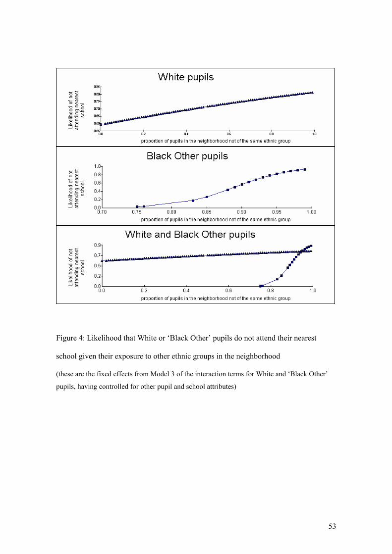
Figure 4: Likelihood that White or ‘Black Other’ pupils do not attend their nearest
school given their exposure to other ethnic groups in the neighborhood
(these are the fixed effects from Model 3 of the interaction terms for White and ‘Black Other’
pupils, having controlled for other pupil and school attributes)
53

Figure 5: Residual variation at the neighborhood level. Above each rank position are the
mean effect and 95% confidence interval for the geodemographic groups having also
allowed for variance at the census OA scale (Model 3). To the right of each (and no
longer in rank order) are shown the equivalent values obtained if variance at the OA
scale is not modeled.
The geodemographic ranks from left to right are: 1 – 7a (Asian Communities); 2 – 6d (Aspiring
Households); 3 – 2a (Transient Communities); 4 – 1c (Older Blue Collar); 5 – 1a (Terraced
Blue Collar); 6 – 4d (Thriving Suburbs); 7 – 6a (Settled Households); 8 – 7b (Afro-Caribbean
Communities); 9 – 5b (Older Workers); 10 – 5a (Senior Communities); 11 – 4b (Prospering
Older Families); 12 – 5c (Public Housing); 13 – 2b (Settled in the City); 14 – 4c (Prospering
Semis); 15 – 1b (Younger Blue Collar); 16 – 6c (Young Families in Terraced Homes); 17 – 3c
(Accessible Countryside); 18 – 6b (Least Divergent); 19 – 4a (Prospering Younger Families)
54

Figure 6: Predicted likelihood (from Model 4) that Indian pupils will not attend their
nearest secondary school
(a) fixed effects only (‘baseline’ probability that an Indian pupil will not attend their nearest
school + amount probability increases given proportion of pupils in the neighborhood who are
not Indian); (b) the same fixed effects plus the variation at the geodemographic level. In both (a)
and (b) the upper line is for Indian pupils living in ‘Asian Communities’ whilst the lower line is
for pupils in all other neighborhood groups.
55