GUIDE TO CONE PENETRATION TESTING - cpt-robertson.com Guide 6th 2015.pdf · Cone penetration test....
140
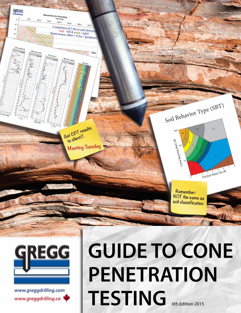
Cone Bearing (bar), Qt 1 10 100 1000 0 1 2 3 4 5 6 7 8 Friction Ratio (%), Rf 1 2 3 11 12 4 5 6 7 8 9 10 E Qt/N SBT 2 Sensitive, fine grained Organic materials y Soil Behavior Type (SBT) Remember: NOT the same as soil classification Get CPT results to client!! Meeting Tuesday www.greggdrilling.com www.greggdrilling.ca GUIDE TO CONE PENETRATION TESTING 6th Edition 2015
Transcript of GUIDE TO CONE PENETRATION TESTING - cpt-robertson.com Guide 6th 2015.pdf · Cone penetration test....
Co
ne
Bea
rin
g (b
ar),
Qt
1
10
100
1000
0 1
2 3 4
5
6 7
8
Friction Ratio (%), Rf1
2
3
1112
45
67
89
10
ZONE Qt/N
S
BT
1
2
Sensitive, fine grained
2
1
Organic materials
3
1
Clay
4
1.5
Silty clay to clay
5
2
Clayey silt to silty clay
6
2.5
Sandy silt to clayey silt
7
3
Silty sand to sandy silt
8
4
Sand to silty sand
9
5
Sand
10
6
Gravelly sand to sand
11
1
Very stiff fine grained*
12
2
Sand to clayey sand*
*over consolidated or cemented
Soil Behavior Type (SBT)
Remember:NOT the same assoil classification
Get CPT results
to client!!
Meeting Tuesday
www.greggdrilling.com
www.greggdrilling.ca
GUIDE TO CONE PENETRATION TESTING 6th Edition 2015

Guide toCone Penetration Testing
forGeotechnical Engineering
By
P. K. Robertsonand
K.L. Cabal (Robertson)
Gregg Drilling & Testing, Inc.
6th EditionDecember 2014

Gregg Drilling & Testing, Inc.Corporate Headquarters2726 Walnut AvenueSignal Hill, California 90755
Telephone: (562) 427-6899Fax: (562) 427-3314E-mail: [email protected]: www.greggdrilling.com
The publisher and the author make no warranties or representations of any kind concerning the accuracy orsuitability of the information contained in this guide for any purpose and cannot accept any legalresponsibility for any errors or omissions that may have been made.
Copyright © 2014 Gregg Drilling & Testing, Inc. All rights reserved.

TABLE OF CONTENTS
Glossary i
Introduction 1
Risk Based Site Characterization 2
Role of the CPT 3
Cone Penetration Test (CPT) 6
Introduction 6
History 7
Test Equipment and Procedures 10
Additional Sensors/Modules 11
Pushing Equipment 12
Depth of Penetration 17
Test Procedures 17
Cone Design 20
CPT Interpretation 24Soil Profiling and Soil Type 25Equivalent SPT N60 Profiles 33Soil Unit Weight () 36Undrained Shear Strength (su) 37Soil Sensitivity 38Undrained Shear Strength Ratio (su/'vo) 39Stress History - Overconsolidation Ratio (OCR) 40In-Situ Stress Ratio (Ko) 41Relative Density (Dr) 42State Parameter () 44
Friction Angle (’) 46Stiffness and Modulus 48Modulus from Shear Wave Velocity 49Estimating Shear Wave Velocity from CPT 50Identification of Unusual Soils Using the SCPT 51Hydraulic Conductivity (k) 52Consolidation Characteristics 55Constrained Modulus 58
Applications of CPT Results 59Shallow Foundation Design 60Deep Foundation Design 83Seismic Design - Liquefaction 96Ground Improvement Compaction Control 121Design of Wick or Sand Drains 124
Software 125
Main References 129


CPT Guide – 2014 Glossary
i
Glossary
This glossary contains the most commonly used terms related to CPT and arepresented in alphabetical order.
CPTCone penetration test.
CPTuCone penetration test with pore pressure measurement – piezoconetest.
ConeThe part of the cone penetrometer on which the cone resistance ismeasured.
Cone penetrometerThe assembly containing the cone, friction sleeve, and any othersensors, as well as the connections to the push rods.
Cone resistance, qc
The force acting on the cone, Qc, divided by the projected area of thecone, Ac.
qc = Qc / Ac
Corrected cone resistance, qt
The cone resistance qc corrected for pore water effects.qt = qc + u2(1- a)
Data acquisition systemThe system used to record the measurements made by the cone.
Dissipation testA test when the decay of the pore pressure is monitored during a pausein penetration.
Filter elementThe porous element inserted into the cone penetrometer to allowtransmission of pore water pressure to the pore pressure sensor, whilemaintaining the correct dimensions of the cone penetrometer.
Friction ratio, Rf
The ratio, expressed as a percentage, of the sleeve friction resistance,fs, to the cone resistance, qt, both measured at the same depth.
Rf = (fs/qt) x 100%
CPT Guide - 2014 Glossary
ii
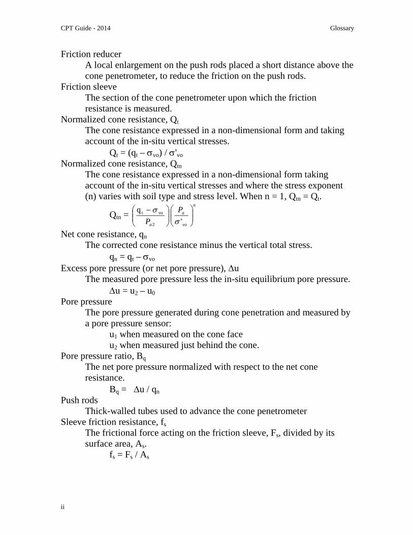
Friction reducerA local enlargement on the push rods placed a short distance above thecone penetrometer, to reduce the friction on the push rods.
Friction sleeveThe section of the cone penetrometer upon which the frictionresistance is measured.
Normalized cone resistance, Qt
The cone resistance expressed in a non-dimensional form and takingaccount of the in-situ vertical stresses.
Qt = (qt – vo) / 'vo
Normalized cone resistance, Qtn
The cone resistance expressed in a non-dimensional form takingaccount of the in-situ vertical stresses and where the stress exponent(n) varies with soil type and stress level. When n = 1, Qtn = Qt.
Qtn =n
vo
a
a
vo P
P
'
q
2
t
Net cone resistance, qn
The corrected cone resistance minus the vertical total stress.qn = qt – vo
Excess pore pressure (or net pore pressure), uThe measured pore pressure less the in-situ equilibrium pore pressure.
u = u2 – u0
Pore pressureThe pore pressure generated during cone penetration and measured bya pore pressure sensor:
u1 when measured on the cone faceu2 when measured just behind the cone.
Pore pressure ratio, Bq
The net pore pressure normalized with respect to the net coneresistance.
Bq = u / qn
Push rodsThick-walled tubes used to advance the cone penetrometer
Sleeve friction resistance, fs
The frictional force acting on the friction sleeve, Fs, divided by itssurface area, As.
fs = Fs / As

CPT Guide – 2014 Introduction
1
Introduction
The purpose of this guide is to provide a concise resource for the applicationof the CPT to geotechnical engineering practice. This guide is a supplementand update to the book ‘CPT in Geotechnical Practice’ by Lunne, Robertsonand Powell (1997). This guide is applicable primarily to data obtained usinga standard electronic cone with a 60-degree apex angle and either a diameterof 35.7 mm or 43.7 mm (10 or 15 cm2 cross-sectional area).
Recommendations are provided on applications of CPT data for soilprofiling, material identification and evaluation of geotechnical parametersand design. The companion book (Lunne et al., 1997) provides more detailson the history of the CPT, equipment, specification and performance. Acompanion Guide to CPT for Geo-environmental Applications is alsoavailable. The companion book also provides extensive background oninterpretation techniques. This guide provides only the basicrecommendations for the application of the CPT for geotechnical design
A list of the main references is included at the end of this guide. A morecomprehensive reference list can be found in the companion CPT book andthe recently listed technical papers. Some recent technical papers can bedownloaded from either www.greggdrilling.com, www.cpt-robertson.com orwww.cpt10.com and www.cpt14.com.
Additional details on CPT interpretation are provided in a series of freewebinars that can be viewed at http://www.greggdrilling.com/webinars. Acopy of the webinar slides can also be downloaded from the same web site.
CPT Guide - 2014 Risk Based Site Characterization
2
Risk Based Site Characterization
Risk and uncertainty are characteristics of the ground and are never fullyeliminated. The appropriate level of sophistication for site characterizationand analyses should be based on the following criteria:
Precedent and local experience Design objectives Level of geotechnical risk Potential cost savings
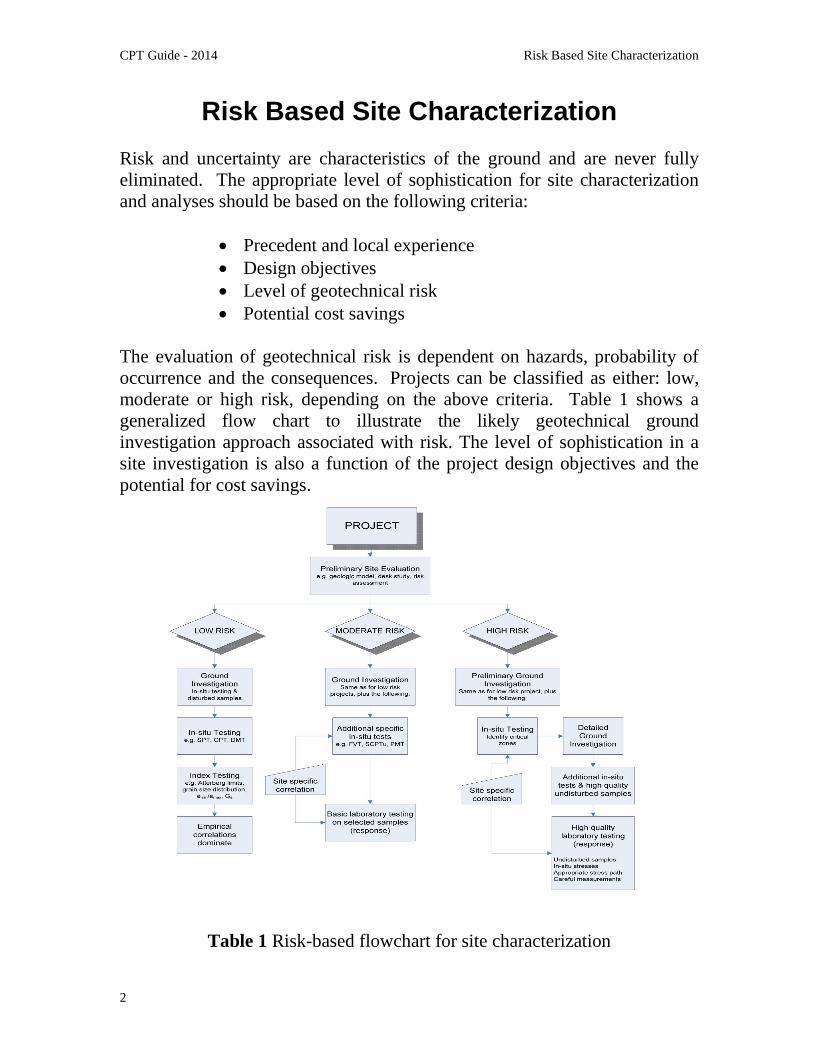
The evaluation of geotechnical risk is dependent on hazards, probability ofoccurrence and the consequences. Projects can be classified as either: low,moderate or high risk, depending on the above criteria. Table 1 shows ageneralized flow chart to illustrate the likely geotechnical groundinvestigation approach associated with risk. The level of sophistication in asite investigation is also a function of the project design objectives and thepotential for cost savings.
Table 1 Risk-based flowchart for site characterization

CPT Guide - 2014 Role of the CPT
3
Role of the CPT
The objectives of any subsurface investigation are to determine the following:
Nature and sequence of the subsurface strata (geologic regime) Groundwater conditions (hydrologic regime) Physical and mechanical properties of the subsurface strata
For geo-environmental site investigations where contaminants are possible, theabove objectives have the additional requirement to determine:
Distribution and composition of contaminants
The above requirements are a function of the proposed project and theassociated risks. An ideal investigation program should include a mix of fieldand laboratory tests depending on the risk of the project.
Table 2 presents a partial list of the major in-situ tests and their perceivedapplicability for use in different ground conditions.
Table 2. The applicability and usefulness of in-situ tests(Lunne, Robertson & Powell, 1997, updated by Robertson, 2012)

CPT Guide - 2014 Role of the CPT
4
The Cone Penetration Test (CPT) and its enhanced versions such as thepiezocone (CPTu) and seismic (SCPT), have extensive applications in a widerange of soils. Although the CPT is limited primarily to softer soils, withmodern large pushing equipment and more robust cones, the CPT can beperformed in stiff to very stiff soils, and in some cases soft rock.
Advantages of CPT: Fast and continuous profiling Repeatable and reliable data (not operator-dependent) Economical and productive Strong theoretical basis for interpretation
Disadvantage of CPT: Relatively high capital investment Requires skilled operators No soil sample, during a CPT Penetration can be restricted in gravel/cemented layers
Although it is not possible to obtain a soil sample during a CPT, it is possible toobtain soil samples using CPT pushing equipment. The continuous nature ofCPT results provides a detailed stratigraphic profile to guide in selectivesampling appropriate for the project. The recommended approach is to firstperform several CPT soundings to define the stratigraphic profile and to provideinitial estimates of geotechnical parameters, then follow with selective sampling.The type and amount of sampling will depend on the project requirements andrisk as well as the stratigraphic profile. Typically sampling will be focused incritical zones as defined by the CPT.
A variety of push-in discrete depth soil samplers are available. Most are basedon designs similar to the original Gouda or MOSTAP soil samplers from theNetherlands. The samplers are pushed to the required depth in a closed position.The Gouda type samplers have an inner cone tip that is retracted to the lockedposition leaving a hollow sampler with small diameter (25mm/1 inch) stainlesssteel or brass sample tubes. The hollow sampler is then pushed to collect asample. The filled sampler and push rods are then retrieved to the groundsurface. The MOSTAP type samplers contain a wire to fix the position of theinner cone tip before pushing to obtain a sample. Modifications have also beenmade to include a wireline system so that soil samples can be retrieved at

CPT Guide - 2014 Role of the CPT
5
multiple depths rather than retrieving and re-deploying the sampler and rods ateach interval. The wireline systems tend to work better in soft soils. Figure 1shows a schematic of typical (Gouda-type) CPT-based soil sampler. The speedof sampling depends on the maximum speed of the pushing equipment but is notlimited to the standard 2cm/s used for the CPT. Some specialized CPT truckscan take samples at a rate of up to 40cm/s. Hence, push-in soil sampling can befast and efficient. In very soft soils, special 0.8m (32 in) long push-in pistonsamplers have been developed to obtain 63mm (2.5 in) diameter undisturbed soilsamples.
Figure 1 Schematic of simple direct-push (CPT-based) soil sampler(www.greggdrilling.com)

CPT Guide - 2014 Cone Penetration Test (CPT)
6
Cone Penetration Test (CPT)
Introduction
In the Cone Penetration Test (CPT), a cone on the end of a series of rods ispushed into the ground at a constant rate and continuous measurements are madeof the resistance to penetration of the cone and of a surface sleeve. Figure 2illustrates the main terminology regarding cone penetrometers.
The total force acting on the cone, Qc, divided by the projected area of the cone,Ac, produces the cone resistance, qc. The total force acting on the frictionsleeve, Fs, divided by the surface area of the friction sleeve, As, produces thesleeve resistance, fs. In a piezocone, pore pressure is also measured, typicallybehind the cone in the u2 location, as shown in Figure 2.
Figure 2 Terminology for cone penetrometers

CPT Guide - 2014 Cone Penetration Test (CPT)
7
History
1932The first cone penetrometer tests were made using a 35 mm outside diameter gaspipe with a 15 mm steel inner push rod. A cone tip with a 10 cm2 projected areaand a 60o apex angle was attached to the steel inner push rods, as shown inFigure 3.
Figure 3 Early Dutch mechanical cone (after Sanglerat, 1972)
1935Delf Soil Mechanics Laboratory designed the first manually operated 10ton(100kN) cone penetration push machine, see Figure 4.
Figure 4 Early Dutch mechanical cone (after Delft Geotechnics)

CPT Guide - 2014 Cone Penetration Test (CPT)
8
1948The original Dutch mechanical cone was improved by adding a conical part justabove the cone. The purpose of the geometry was to prevent soil from enteringthe gap between the casing and inner rods. The basic Dutch mechanical cones,shown in Figure 5, are still in use in some parts of the world.
Figure 5 Dutch mechanical cone penetrometer with conical mantle
1953A friction sleeve (‘adhesion jacket’) was added behind the cone to includemeasurement of the local sleeve friction (Begemann, 1953), see Figure 6.Measurements were made every 20 cm, (8 inches) and for the first time, frictionratio was used to classify soil type (see Figure 7).
Figure 6 Begemann type cone with friction sleeve

CPT Guide - 2014 Cone Penetration Test (CPT)
9
Figure 7 First CPT-based soil classification for Begemann mechanical cone
1965Fugro developed an electric cone, of which the shape and dimensions formedthe basis for the modern cones and the International Reference Test and ASTMprocedure. The main improvements relative to the mechanical conepenetrometers were:
Elimination of incorrect readings due to friction between inner rods andouter rods and weight of inner rods.
Continuous testing with continuous rate of penetration without the needfor alternate movements of different parts of the penetrometer and noundesirable soil movements influencing the cone resistance.
Simpler and more reliable electrical measurement of cone resistance andsleeve friction resistance.
1974Cone penetrometers that could also measure pore pressure (piezocones) wereintroduced. Early designs had various shapes and pore pressure filter locations.Gradually the practice has become more standardized so that the recommendedposition of the filter element is close behind the cone at the u2 location. With themeasurement of pore water pressure it became apparent that it was necessary tocorrect the cone resistance for pore water pressure effects (qt), especially in softclay.

CPT Guide - 2014 Cone Penetration Test (CPT)
10
Test Equipment and Procedures
Cone Penetrometers
Cone penetrometers come in a range of sizes with the 10 cm2 and 15 cm2 probesthe most common and specified in most standards. Figure 8 shows a range ofcones from a mini-cone at 2 cm2 to a large cone at 40 cm2. The mini cones areused for shallow investigations, whereas the large cones can be used in gravelysoils.
Figure 8 Range of CPT probes (from left: 2 cm2, 10 cm2, 15 cm2, 40 cm2)

CPT Guide - 2014 Cone Penetration Test (CPT)
11
Additional Sensors/Modules
Since the introduction of the electric cone in the early 1960’s, many additionalsensors have been added to the cone, such as;
Temperature Geophones/accelerometers (seismic wave velocity) Pressuremeter (cone pressuremeter) Camera (visible light) Radioisotope (gamma/neutron) Electrical resistivity/conductivity Dielectric pH Oxygen exchange (redox) Laser/ultraviolet induced fluorescence (LIF/UVOST) Membrane interface probe (MIP)
The latter items are primarily for geo-environmental applications.One of the more common additional sensors is a geophone or accelerometer toallow the measurement of seismic wave velocities. A schematic of the seismicCPT (SCPT) procedure is shown in Figure 9.
Figure 9 Schematic of Seismic CPT (SCPT) test procedure

CPT Guide - 2014 Cone Penetration Test (CPT)
12
Pushing Equipment
Pushing equipment consists of push rods, a thrust mechanism and a reactionframe.
On Land
Pushing equipment for land applications generally consist of specially built unitsthat are either truck or track mounted. CPT’s can also be carried out using ananchored drill-rig. Figures 10 to 13 show a range of on land pushing equipment.
Figure 10 Truck mounted 25 ton CPT unit

CPT Guide - 2014 Cone Penetration Test (CPT)
13
Figure 11 Track mounted 20 ton CPT unit
Figure 12 Small anchored drill-rig unit

CPT Guide - 2014 Cone Penetration Test (CPT)
14
Figure 13 Portable ramset for CPT inside buildings or limited access
Figure 14 Mini-CPT system attached to small track mounted auger rig
CPT Guide - 2014 Cone Penetration Test (CPT)
15
Over Water
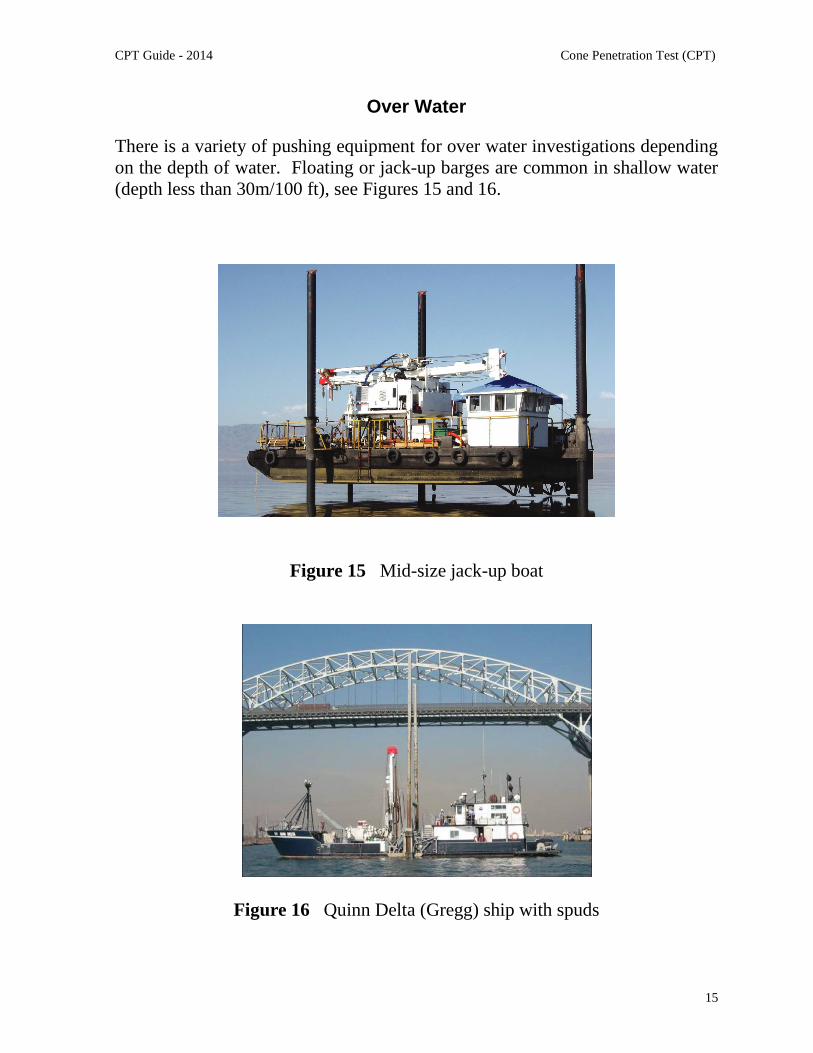
There is a variety of pushing equipment for over water investigations dependingon the depth of water. Floating or jack-up barges are common in shallow water(depth less than 30m/100 ft), see Figures 15 and 16.
Figure 15 Mid-size jack-up boat
Figure 16 Quinn Delta (Gregg) ship with spuds

CPT Guide - 2014 Cone Penetration Test (CPT)
16
In deeper water (>100m, 350ft) it is common to place the CPT pushingequipment on the seafloor using specially designed underwater systems, such asshown in Figure 17. Seabed systems can push full size cones (10 and 15cm2
cones) and smaller systems for mini-cones (2 and 5cm2 cones) using continuouspushing systems.
Figure 17 (Gregg) Seafloor CPT system for pushing full size cones in verydeep water (up to 4,000msw)
Alternatively, it is also possible to push the CPT from the bottom of a boreholeusing down-hole equipment. The advantage of down-hole CPT in a drilledborehole is that much deeper penetration can be achieved and hard layers can bedrilled through. Down-hole methods can be applied both on-shore and off-shore. Recently, remotely controlled seabed drill rigs have been developed thatcan drill and sample and push CPT in up to 4,000m (13,000 ft) of water (e.g.Lunne, 2010).

CPT Guide - 2014 Cone Penetration Test (CPT)
17
Depth of Penetration
CPT’s can be performed to depths exceeding 100m (300ft) in soft soils and withlarge capacity pushing equipment. To improve the depth of penetration, thefriction along the push rods should be reduced. This can be done using anexpanded coupling (i.e. friction reducer) a short distance, typically 1m (3ft),behind the cone. Penetration will be limited if, very hard soils, gravel layers orrock are encountered. It is common to use 15cm2 cones to increase penetrationdepth, since 15cm2 cones are more robust and have a slightly larger diameterthan the standard 10cm2 push rods. The push rods can also be lubricated withdrilling mud to remove rod friction for deep soundings. Depth of penetrationcan also be increased using down-hole techniques with a drill rig.
Test Procedures
Pre-drilling
For penetration in fills or hard soils it may be necessary to pre-drill in order toavoid damaging the cone. Pre-drilling, in certain cases, may be replaced byfirst pre-punching a hole through the upper problem material with a solid steel‘dummy’ probe with a diameter slightly larger than the cone. It is also commonto hand auger the first 1.5m (5ft) in urban areas to avoid underground utilities.
Verticality
The thrust machine should be set up so as to obtain a thrust direction as near aspossible to vertical. The deviation of the initial thrust direction from verticalshould not exceed 2 degrees and push rods should be checked for straightness.Modern cones have simple slope sensors incorporated to enable a measure ofthe non-verticality of the sounding. This is useful to avoid damage toequipment and breaking of push rods. For depths less than 15m (50ft),significant non-verticality is unusual, provided the initial thrust direction isvertical.

CPT Guide - 2014 Cone Penetration Test (CPT)
18
Reference Measurements
Modern cones have the potential for a high degree of accuracy and repeatability(~0.1% of full-scale output). Tests have shown that the output of the sensors atzero load can be sensitive to changes in temperature, although most cones nowinclude some temperature compensation. It is common practice to record zeroload readings of all sensors to track these changes. Zero load readings should bemonitored and recorded at the start and end of each CPT.
Rate of Penetration
The standard rate of penetration is 2cm/s (approximately 1in/s). Hence, a 20m(60ft) sounding can be completed (start to finish) in about 30 minutes. The CPTresults are generally not sensitive to slight variations in the rate of penetration.
Interval of readings
Electric cones produce continuous analogue data. However, most systemsconvert the data to digital form at selected intervals. Most standards require theinterval to be no more than 200mm (8in). In general, most systems collect dataat intervals of between 10 - 50mm, with 20 mm (~1in) being the more common.
Dissipation Tests
During a pause in penetration, any excess pore pressure generated around thecone will start to dissipate. The rate of dissipation depends upon the coefficientof consolidation, which in turn, depends on the compressibility and permeabilityof the soil. The rate of dissipation also depends on the diameter of the probe. Adissipation test can be performed at any required depth by stopping thepenetration and measuring the decay of pore pressure with time. It is commonto record the time to reach 50% dissipation (t50), as shown in Figure 18. If theequilibrium pore pressure is required, the dissipation test should continue untilno further dissipation is observed. This can occur rapidly in sands, but may takemany hours in plastic clays. Dissipation rate increases as probe size decreases.

CPT Guide - 2014 Cone Penetration Test (CPT)
19
Figure 18 Example dissipation test to determine t50
Calibration and Maintenance
Calibrations should be carried out at intervals based on the stability of the zeroload readings. Typically, if the zero load readings remain stable, the load cellsdo not require a check calibration. For major projects, check calibrations can becarried out before and after the field work, with functional checks during thework. Functional checks should include recording and evaluating the zero loadmeasurements (baseline readings).
With careful design, calibration, and maintenance, strain gauge load cells andpressure transducers can have an accuracy and repeatability of better than +/-0.1% of full-scale reading.
Table 3 shows a summary of checks and recalibrations for the CPT.

CPT Guide - 2014 Cone Penetration Test (CPT)
20
MaintenanceStart
ofProject
Start ofTest
End ofTest
End ofDay
Once aMonth
Every 3months*
Wear x x x
O-ring seals x x
Push-rods x x
Pore pressure-filter
x x
Calibration x*
Computer x
Cone x
Zero-load x x
Cables x x
Table 3 Summary of checks and recalibrations for the CPT
*Note: recalibrations are normally carried out only when the zero-load readings drift outside manufacturesrecommended range
Cone Design
Penetrometers use strain gauge load cells to measure the resistance topenetration. Basic cone designs use either separate load cells or subtractionload cells to measure the tip resistance (qc) and sleeve resistance (fs). Insubtraction cones the sleeve friction is derived by ‘subtracting’ the tip load fromthe tip + friction load. Figure 19 illustrates the general principle behind load celldesigns using either separated load cells or subtraction load cells.

CPT Guide - 2014 Cone Penetration Test (CPT)
21
Figure 19 Designs for cone penetrometers (a) tip and sleeve friction load cellsin compression, (b) tip load cell in compression and sleeve friction loadcell in tension, (c) subtraction type load cell design (after Lunne et al.,1997)
In the 1980’s subtraction cones became popular because of the overallrobustness of the penetrometer. However, in soft soils, subtraction conedesigns suffer from a lack of accuracy in the determination of sleeve resistancedue primarily to variable zero load stability of the two load cells. In subtractioncone designs, different zero load errors can produce cumulative errors in thederived sleeve resistance values. For accurate sleeve resistance measurementsin soft sediments, it is recommended that cones have separate (compression)load cells.
With good design (separate load cells, equal end area friction sleeve) and qualitycontrol (zero load measurements, tolerances and surface roughness) it is possibleto obtain repeatable tip and sleeve resistance measurements. However, fs
measurements, in general, will be less accurate than tip resistance, qc, in mostsoft fine-grained soils.

CPT Guide - 2014 Cone Penetration Test (CPT)
22
Pore pressure (water) effects
Due to the inner geometry of the cone the ambient water pressure acts on theshoulder behind the cone and on the ends of the friction sleeve. This effect isoften referred to as the unequal end area effect (Campanella et al., 1982). Figure20 illustrates the key features for water pressure acting behind the cone and onthe end areas of the friction sleeve. In soft clays and silts and in over waterwork, the measured qc must be corrected for pore water pressures acting on thecone geometry, thus obtaining the corrected cone resistance, qt:
qt = qc + u2 (1 – a)
Where ‘a’ is the net area ratio determined from laboratory calibration with atypical value between 0.70 and 0.85. In sandy soils qc = qt.
Figure 20 Unequal end area effects on cone tip and friction sleeve

CPT Guide - 2014 Cone Penetration Test (CPT)
23
A similar correction should be applied to the sleeve friction.
ft = fs – (u2Asb – u3Ast)/As
where: fs = measured sleeve frictionu2 = water pressure at base of sleeveu3 = water pressure at top of sleeveAs = surface area of sleeveAsb = cross-section area of sleeve at baseAst = cross-sectional area of sleeve at top
However, the ASTM standard requires that cones have an equal end area frictionsleeve (i.e. Ast = Asb) that reduces the need for such a correction. For 15cm2
cones, where As is large compared to Asb and Ast, (and Ast = Asb) the correctionis generally small. All cones should have equal end area friction sleeves tominimize the effect of water pressure on the sleeve friction measurements.Careful monitoring of the zero load readings is also required.
In the offshore industry, where CPT can be carried out in very deep water (>1,000m), cones are sometimes compensated (filled with oil) so that the pressureinside the cone is equal to the hydrostatic water pressure outside the cone. Forcompensated cones the correction for cone geometry to obtain qt is slightlydifferent than shown above, since the cone can record zero qc at the mudline.

CPT Guide - 2014 Cone Penetration Test (CPT)
24
CPT Interpretation
Numerous semi-empirical correlations have been developed to estimategeotechnical parameters from the CPT for a wide range of soils. Thesecorrelations vary in their reliability and applicability. Because the CPT hasadditional sensors (e.g. pore pressure, CPTu and seismic, SCPT), theapplicability to estimate soil parameters varies. Since CPT with pore pressuremeasurements (CPTu) is commonly available, Table 4 shows an estimate of theperceived applicability of the CPTu to estimate soil parameters. If seismic isadded, the ability to estimate soil stiffness (E, G & Go) improves further.
Soil Type Dr
Ko OCR St su
' E, G* M G0
* k ch
Coarse-gained(sand)
2-3 2-3 5 5 2-3 2-3 2-3 2-3 3-4 3-4
Fine-grained(clay)
2 1 2 1-2 4 2-4 2-3 2-4 2-3 2-3
Table 4 Perceived applicability of CPTu for deriving soil parameters
1=high, 2=high to moderate, 3=moderate, 4=moderate to low, 5=low reliability, Blank=no applicability, *improved with SCPT
Where:Dr Relative density ' Peak friction angle State Parameter K0 In-situ stress ratioE, G Young’s and Shear moduli G0 Small strain shear moduliOCR Over consolidation ratio M 1-D Compressibilitysu Undrained shear strength St Sensitivitych Coefficient of consolidation k Permeability
Most semi-empirical correlations apply primarily to relatively young,uncemented, silica-based soils.

CPT Guide - 2014 Cone Penetration Test (CPT)
25
Soil Profiling and Soil Type
One of the major applications of the CPT is for soil profiling and soil type.Typically, the cone resistance, (qt) is high in sands and low in clays, and thefriction ratio (Rf = fs/qt) is low in sands and high in clays. The CPT cannot beexpected to provide accurate predictions of soil type based on physicalcharacteristics, such as, grain size distribution but provide a guide to themechanical characteristics (strength, stiffness, compressibility) of the soil, orthe soil behavior type (SBT). CPT data provides a repeatable index of theaggregate behavior of the in-situ soil in the immediate area of the probe. Hence,prediction of soil type based on CPT is referred to as Soil Behavior Type (SBT).
Non-Normalized SBT Charts
The most commonly used CPT soil behavior type (SBT) chart was suggested byRobertson et al. (1986), the updated, dimensionless version (Robertson, 2010) isshown in Figure 21. This chart uses the basic CPT parameters of coneresistance, qt and friction ratio, Rf. The chart is global in nature and can providereasonable predictions of soil behavior type for CPT soundings up to about 20m(60ft) in depth. Overlap in some zones should be expected and the zones can bemodified somewhat based on local experience.
Normalized SBTn Charts
Since both the penetration resistance and sleeve resistance increase with depthdue to the increase in effective overburden stress, the CPT data requiresnormalization for overburden stress for very shallow and/or very deepsoundings.
A popular CPT soil behavior chart based on normalized CPT data is that firstproposed by Robertson (1990) and shown in Figure 22. A zone has beenidentified in which the CPT results for most young, un-cemented, insensitive,normally consolidated soils will plot. The chart identifies general trends inground response, such as, increasing soil density, OCR, age and cementation forsandy soils, increasing stress history (OCR) and soil sensitivity (St) for cohesivesoils. Again the chart is global in nature and provides only a guide to soilbehavior type (SBT). Overlap in some zones should be expected and the zonescan be modified somewhat based on local experience.

CPT Guide - 2014 Cone Penetration Test (CPT)
26
Zone Soil Behavior Type
123456789
Sensitive, fine grainedOrganic soils - clay
Clay – silty clay to claySilt mixtures – clayey silt to silty clay
Sand mixtures – silty sand to sandy siltSands – clean sand to silty sand
Gravelly sand to dense sandVery stiff sand to clayey sand*
Very stiff fine grained*
* Heavily overconsolidated or cemented
Pa = atmospheric pressure = 100 kPa = 1 tsf
Figure 21 Non-normalized CPT Soil Behavior Type (SBT) chart(Robertson et al., 1986, updated by Robertson, 2010).

CPT Guide - 2014 Cone Penetration Test (CPT)
27
Zone Soil Behavior Type Ic
1 Sensitive, fine grained N/A2 Organic soils – clay > 3.63 Clays – silty clay to clay 2.95 – 3.64 Silt mixtures – clayey silt to silty clay 2.60 – 2.95
5 Sand mixtures – silty sand to sandy silt 2.05 – 2.6
6 Sands – clean sand to silty sand 1.31 – 2.057 Gravelly sand to dense sand < 1.318 Very stiff sand to clayey sand* N/A9 Very stiff, fine grained* N/A
* Heavily overconsolidated or cemented
Figure 22 Normalized CPT Soil Behavior Type (SBTn) chart, Qt - F(Robertson, 1990, updated by Robertson, 2010).

CPT Guide - 2014 Cone Penetration Test (CPT)
28
The full normalized SBTn charts suggested by Robertson (1990) also included anadditional chart based on normalized pore pressure parameter, Bq, as shown onFigure 23, where;
Bq = u / qn
and; excess pore pressure, u = u2 – u0
net cone resistance, qn = qt – vo
The Qt – Bq chart can aid in the identification of soft, saturated fine-grained soilswhere excess CPT penetration pore pressures can be large. In general, the Qt -Bq chart is not commonly used for onshore CPT due to the lack of repeatabilityof the pore pressure results (e.g. poor saturation or loss of saturation of the filterelement, etc.).
Figure 23 Normalized CPT Soil Behavior Type (SBTn) chartsQt – Fr and Qt - Bq (after Robertson, 1990).

CPT Guide - 2014 Cone Penetration Test (CPT)
29
If no prior CPT experience exists in a given geologic environment it is advisableto obtain samples from appropriate locations to verify the soil type. Ifsignificant CPT experience is available and the charts have been evaluated basedon this experience, samples may not always be required.
Soil behavior type can be improved if pore pressure measurements are alsocollected, as shown on Figure 23. In soft clays and silts the penetration porepressures can be very large, whereas, in stiff heavily over-consolidated clays ordense silts and silty sands the penetration pore pressures (u2) can be small andsometimes negative relative to the equilibrium pore pressures (u0). The rate ofpore pressure dissipation during a pause in penetration can also guide in the soiltype. In sandy soils any excess pore pressures will dissipate very quickly,whereas, in clays the rate of dissipation can be very slow.
To simplify the application of the CPT SBTn chart shown in Figure 22, thenormalized cone parameters Qt and Fr can be combined into one Soil BehaviorType index, Ic, where Ic is the radius of the essentially concentric circles thatrepresent the boundaries between each SBTn zone. Ic can be defined as follows;
Ic = ((3.47 - log Qt)2 + (log Fr + 1.22)2)0.5
where:Qt = normalized cone penetration resistance (dimensionless)
= (qt – vo)/'vo
Fr = normalized friction ratio, in %= (fs/(qt – vo)) x 100%
The term Qt represents the simple normalization with a stress exponent (n) of1.0, which applies well to clay-like soils. Robertson (2009) suggested that thenormalized SBTn charts shown in Figures 22 and 23 should be used with thenormalized cone resistance (Qtn) calculated using a stress exponent that varieswith soil type via Ic (i.e. Qtn, see Figure 46 for details).
The approximate boundaries of soil behavior types are then given in terms of theSBTn index, Ic, as shown in Figure 22. The soil behavior type index does notapply to zones 1, 8 and 9. Profiles of Ic provide a simple guide to the continuousvariation of soil behavior type in a given soil profile based on CPT results.Independent studies have shown that the normalized SBTn chart shown in Figure22 typically has greater than 80% reliability when compared with samples.

CPT Guide - 2014 Cone Penetration Test (CPT)
30
Schneider et al (2008) proposed a CPT-based soil type chart based onnormalized cone resistance (Qt) and normalized excess pore pressure (u2/'vo),as shown on Figure 24. Superimposed on the Schneider et al chart are contoursof Bq to illustrate the link with u2/'vo. Also shown on the Schneider et al chartare approximate contours of OCR (dashed lines). Application of the Schneideret al chart can be problematic for some onshore projects where the CPTu porepressure results may not be reliable, due to loss of saturation. However, foroffshore projects, where CPTu sensor saturation is more reliable, and onshoreprojects in soft fine-grained soils with high groundwater, the chart can be veryhelpful. The Schneider et al chart is focused primarily on fine-grained soils wereexcess pore pressures are recorded and Qt is small.
Figure 24 CPT classification chart from Schneider et al (2008) based on(u2/’vo) with contours of Bq and OCR
In recent years, the SBT charts have been color coded to aid in the visualpresentation of SBT on a CPT profile. An example CPTu profile is shown inFigure 25.

CPT Guide - 2014 Cone Penetration Test (CPT)
31
Figure 25 Examples of (a) CPTu and (b) SCPTu(1 tsf ~ 0.1 MPa, 14.5 psi = 100kPa, 1ft = 0.3048m)

CPT Guide - 2014 Cone Penetration Test (CPT)
32
A more general normalized CPT SBT chart, using large strain ‘soil behavior’descriptions, is shown in Figure 26.
Figure 26 Normalized CPT Soil Behavior Type (SBTn) chart, Qt - Fusing general large strain ‘soil behavior’ descriptors
(Modified from Robertson, 2012)
CD Coarse-grained Dilative soil – predominately drained CPTCC Coarse-grained Contractive soil – predominately drained CPTFD Fine-grained Dilative soil – predominately undrained CPTFC Fine-grained Contractive – predominately undrained CPT

CPT Guide - 2014 Cone Penetration Test (CPT)
33
Equivalent SPT N60 Profiles
The Standard Penetration Test (SPT) is one of the most commonly used in-situtests in many parts of the world, especially North and South America. Despitecontinued efforts to standardize the SPT procedure and equipment there are stillproblems associated with its repeatability and reliability. However, manygeotechnical engineers have developed considerable experience with designmethods based on local SPT correlations. When these engineers are firstintroduced to the CPT they initially prefer to see CPT results in the form ofequivalent SPT N-values. Hence, there is a need for reliable CPT/SPTcorrelations so that CPT data can be used in existing SPT-based designapproaches.
There are many factors affecting the SPT results, such as borehole preparationand size, sampler details, rod length and energy efficiency of the hammer-anvil-operator system. One of the most significant factors is the energy efficiency ofthe SPT system. This is normally expressed in terms of the rod energy ratio(ERr). An energy ratio of about 60% has generally been accepted as thereference value that represents the approximate historical average SPT energy.
A number of studies have been presented over the years to relate the SPT Nvalue to the CPT cone penetration resistance, qc. Robertson et al. (1983)reviewed these correlations and presented the relationship shown in Figure 26relating the ratio (qc/pa)/N60 with mean grain size, D50 (varying between0.001mm to 1mm). Values of qc are made dimensionless when dividing by theatmospheric pressure (pa) in the same units as qc. It is observed that the ratioincreases with increasing grain size.
The values of N used by Robertson et al. correspond to an average energy ratioof about 60%. Hence, the ratio applies to N60, as shown on Figure 27. Otherstudies have linked the ratio between the CPT and SPT with fines content forsandy soils.

CPT Guide - 2014 Cone Penetration Test (CPT)
34
Figure 27 CPT-SPT correlations with mean grain size(Robertson et al., 1983)
The above correlations require the soil grain size information to determine themean grain size (or fines content). Grain characteristics can be estimateddirectly from CPT results using soil behavior type (SBT) charts. The CPT SBTcharts show a clear trend of increasing friction ratio with increasing finescontent and decreasing grain size. Robertson et al. (1986) suggested (qc/pa)/N60
ratios for each soil behavior type zone using the non-normalized CPT chart.
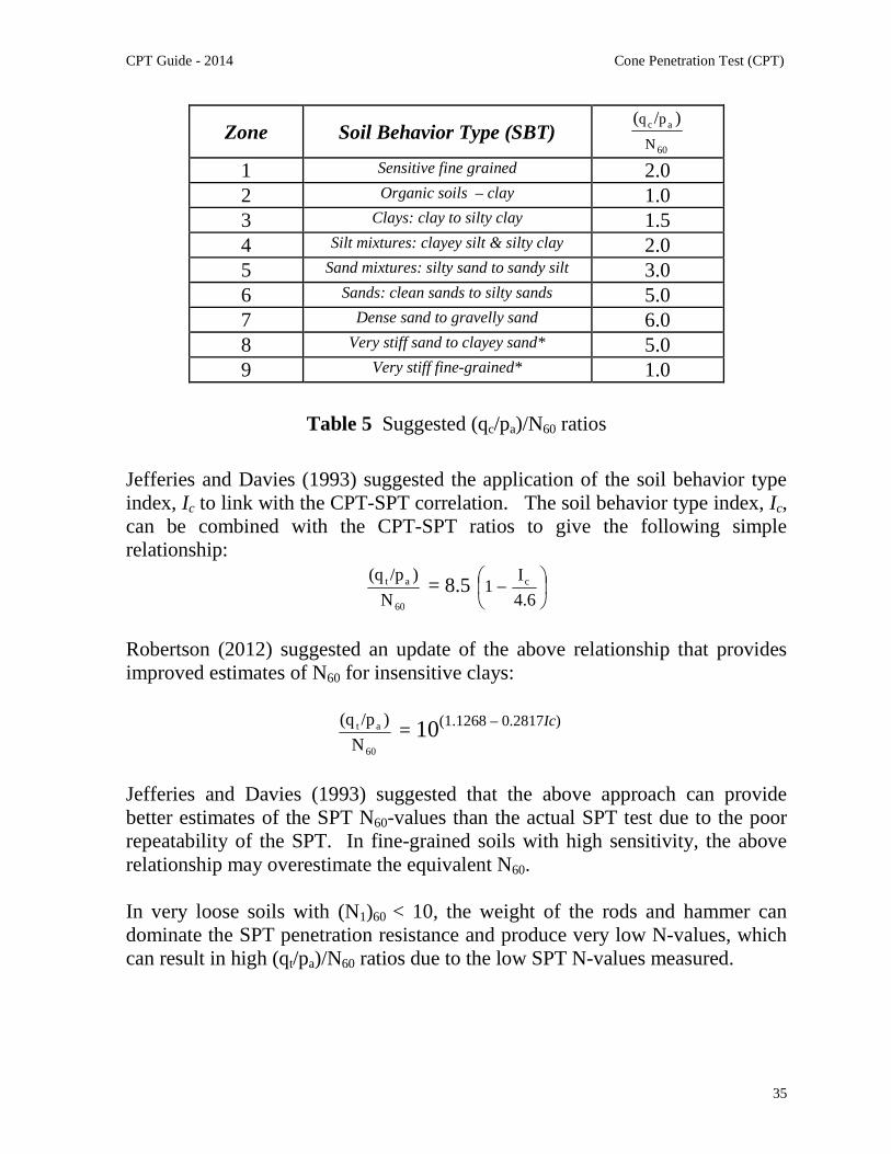
The suggested (qc/pa)/N60 ratio for each soil behavior type is given in Table 5.
These values provide a reasonable estimate of SPT N60 values from CPT data.For simplicity the above correlations are given in terms of qc. For fine grainedsoft soils the correlations should be applied to total cone resistance, qt. Note thatin sandy soils qc = qt.
One disadvantage of this simplified approach is the somewhat discontinuousnature of the conversion. Often a soil will have CPT data that cover differentSBT zones and hence produces discontinuous changes in predicted SPT N60
values.
CPT Guide - 2014 Cone Penetration Test (CPT)
35
Zone Soil Behavior Type (SBT)60
ac
N
pq )/(
1 Sensitive fine grained 2.02 Organic soils – clay 1.03 Clays: clay to silty clay 1.54 Silt mixtures: clayey silt & silty clay 2.05 Sand mixtures: silty sand to sandy silt 3.06 Sands: clean sands to silty sands 5.07 Dense sand to gravelly sand 6.08 Very stiff sand to clayey sand* 5.09 Very stiff fine-grained* 1.0
Table 5 Suggested (qc/pa)/N60 ratios
Jefferies and Davies (1993) suggested the application of the soil behavior typeindex, Ic to link with the CPT-SPT correlation. The soil behavior type index, Ic,can be combined with the CPT-SPT ratios to give the following simplerelationship:
60
at
N
)/p(q= 8.5
4.6
I1 c
Robertson (2012) suggested an update of the above relationship that providesimproved estimates of N60 for insensitive clays:
60
at
N
)/p(q= 10(1.1268 – 0.2817Ic)
Jefferies and Davies (1993) suggested that the above approach can providebetter estimates of the SPT N60-values than the actual SPT test due to the poorrepeatability of the SPT. In fine-grained soils with high sensitivity, the aboverelationship may overestimate the equivalent N60.
In very loose soils with (N1)60 < 10, the weight of the rods and hammer candominate the SPT penetration resistance and produce very low N-values, whichcan result in high (qt/pa)/N60 ratios due to the low SPT N-values measured.
CPT Guide - 2014 Cone Penetration Test (CPT)
36
Soil Unit Weight ()
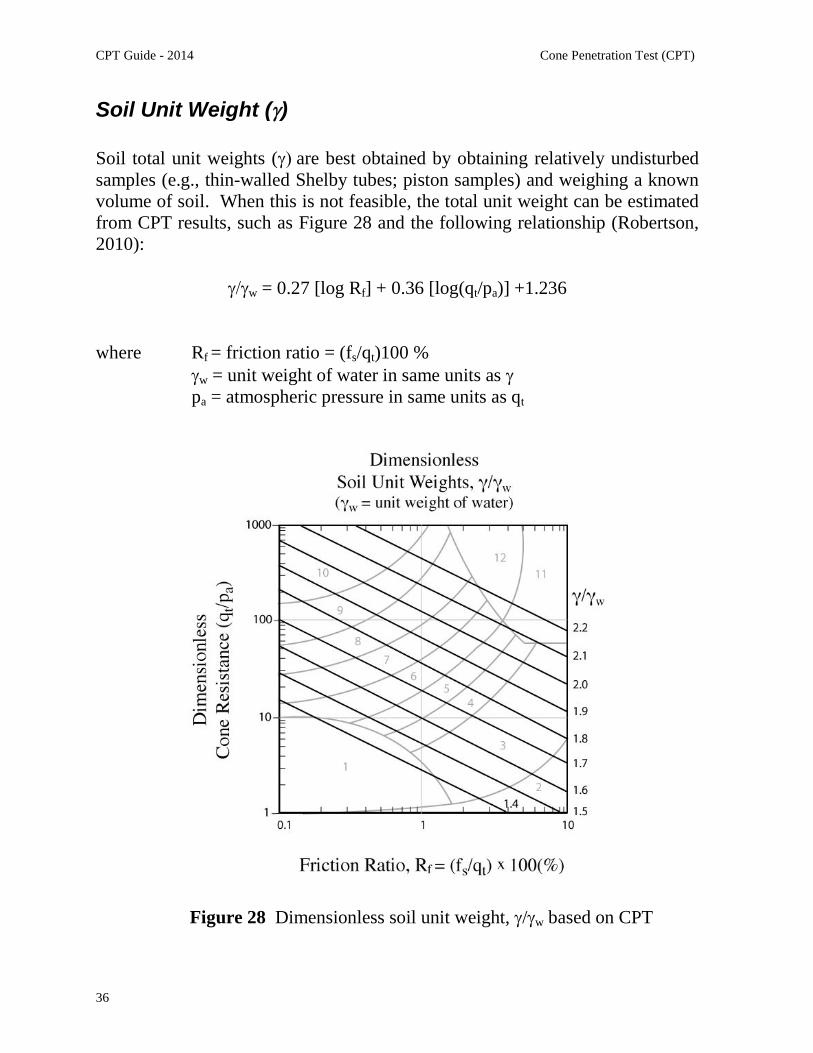
Soil total unit weights (are best obtained by obtaining relatively undisturbedsamples (e.g., thin-walled Shelby tubes; piston samples) and weighing a knownvolume of soil. When this is not feasible, the total unit weight can be estimatedfrom CPT results, such as Figure 28 and the following relationship (Robertson,2010):
w = 0.27 [log Rf] + 0.36 [log(qt/pa)] +1.236
where Rf = friction ratio = (fs/qt)100 %w = unit weight of water in same units as pa = atmospheric pressure in same units as qt
Figure 28 Dimensionless soil unit weight, /w based on CPT

CPT Guide - 2014 Cone Penetration Test (CPT)
37
Undrained Shear Strength (su)
No single value of undrained shear strength, su, exists, since the undrainedresponse of soil depends on the direction of loading, soil anisotropy, strain rate,and stress history. Typically the undrained strength in tri-axial compression islarger than in simple shear that is larger than tri-axial extension (suTC > suSS >suTE). The value of su to be used in analysis therefore depends on the designproblem. In general, the simple shear direction of loading often represents theaverage undrained strength (suSS ~ su(ave)).
Since anisotropy and strain rate will inevitably influence the results of all in-situtests, their interpretation will necessarily require some empirical content toaccount for these factors, as well as possible effects of sample disturbance.
Theoretical solutions have provided valuable insight into the form of therelationship between cone resistance and su. All theories result in a relationshipbetween corrected cone resistance, qt, and su of the form:
su =kt
vt
N
q
Typically Nkt varies from 10 to 18, with 14 as an average for su(ave). Nkt tends toincrease with increasing plasticity and decrease with increasing soil sensitivity.Lunne et al., 1997 showed that Nkt decreases as Bq increases. In very sensitivefine-grained soil, where Bq ~ 1.0, Nkt can be as low as 6.
For deposits where little experience is available, estimate su using the correctedcone resistance (qt) and preliminary cone factor values (Nkt) from 14 to 16. Fora more conservative estimate, select a value close to the upper limit.
In very soft clays, where there may be some uncertainty with the accuracy in qt,estimates of su can be made from the excess pore pressure (u) measured behindthe cone (u2) using the following:
su =Du
NDu
CPT Guide - 2014 Cone Penetration Test (CPT)
38
Where Nu varies from 4 to 10. For a more conservative estimate, select a value
close to the upper limit. Note that Nu is linked to Nkt, via Bq, where:
Nu = Bq Nkt
If previous experience is available in the same deposit, the values suggestedabove should be adjusted to reflect this experience.
For larger, moderate to high risk projects, where high quality field andlaboratory data may be available, site-specific correlations should be developedbased on appropriate and reliable values of su.
Soil Sensitivity
The sensitivity (St) of clay is defined as the ratio of undisturbed peak undrainedshear strength to totally remolded undrained shear strength.
The remolded undrained shear strength, su(Rem), can be assumed equal to thesleeve resistance, fs. Therefore, the sensitivity of a clay can be estimated bycalculating the peak su from either site specific or general correlations with qt oru and su(Rem) from fs, and can be approximated using the following:
St =(Rem)u
u
s
s=
kt
vt
N
q (1 / fs) = 7 / Fr
For relatively sensitive clays (St > 10), the value of fs can be very low withinherent difficulties in accuracy. Hence, the estimate of sensitivity (andremolded strength) should be used as a guide only.

CPT Guide - 2014 Cone Penetration Test (CPT)
39
Undrained Shear Strength Ratio (su/'vo)
It is often useful to estimate the undrained shear strength ratio from the CPT,since this relates directly to overconsolidation ratio (OCR). Critical State SoilMechanics presents a relationship between the undrained shear strength ratio fornormally consolidated clays under different directions of loading and theeffective stress friction angle, '. Hence, a better estimate of undrained shearstrength ratio can be obtained with knowledge of the friction angle [(su /'vo)NC
increases with increasing ']. For normally consolidated clays:
(su /'vo)NC ~ 0.22 in direct simple shear (' = 26o)
From the CPT:
(su /'vo) =q t - svo
s'vo
æ
èç
ö
ø÷ (1/Nkt) = Qt / Nkt
Since Nkt ~ 14 (su /'vo) ~ 0.071 Qt
For a normally consolidated clay where (su /'vo)NC ~ 0.22;
Qt = 3 to 4 for NC insensitive clay
Based on the assumption that the sleeve resistance, fs, is a direct measure of theremolded shear strength, su(Rem) = fs
Therefore:
su(Rem) /'vo = fs /'vo = (F . Qt) / 100
Hence, it is possible to represent (su(Rem)/'vo) contours on the normalized SBTn
chart (Robertson, 2009). These contours also represent OCR for insensitiveclays with high values of (su /'vo) and sensitivity for low values of (su /'vo).

CPT Guide - 2014 Cone Penetration Test (CPT)
40
Stress History - Overconsolidation Ratio (OCR)
Overconsolidation ratio (OCR) is defined as the ratio of the maximum pasteffective consolidation stress and the present effective overburden stress:
OCR =s'ps'vo
For mechanically overconsolidated soils where the only change has been theremoval of overburden stress, this definition is appropriate. However, forcemented and/or aged soils the OCR may represent the ratio of the yield stressand the present effective overburden stress. The yield stress ratio (YSR) willalso depend on the direction and type of loading. For overconsolidated clays:
(su /'vo)OC = (su /'vo)NC (OCR)0.8
Based on this, Robertson (2009) suggested:
OCR = 0.25 (Qt)1.25
Kulhawy and Mayne (1990) suggested a simpler method:
OCR = kq t - svo
s'vo
æ
èç
ö
ø÷= k Qt or 'p = k (qt – vo)
An average value of k = 0.33 can be assumed, with an expected range of 0.2 to0.5. Higher values of k are recommended in aged, heavily overconsolidatedclays. If previous experience is available in the same deposit, the values of kshould be adjusted to reflect this experience and to provide a more reliableprofile of OCR. The simpler Kulhawy and Mayne approach is valid for Qt < 20.For larger, moderate to high-risk projects, where additional high quality fieldand laboratory data may be available, site-specific correlations should bedeveloped based on consistent and relevant values of OCR.
Mayne (2012) suggested an extension of this approach that can be applied to allsoils based on the following: 'p = 0.33(qt – vo)
m (pa/100)1-m
where m is a function of SBT Ic (m ~ 0.72 in young, uncemented silicasand and m ~ 1.0 in intact clay).

CPT Guide - 2014 Cone Penetration Test (CPT)
41
In-Situ Stress Ratio (Ko)
There is no reliable method to determine Ko from CPT. However, an estimatecan be made in fine-grained soils based on an estimate of OCR, as shown inFigure 29.
Kulhawy and Mayne (1990) suggested a simpler approach, using:
Ko = (1 – sin’) (OCR)sin’
That can be approximated (for low plastic fine-grained soils) to:
Ko ~ 0.5 (OCR) 0.5
These approaches are generally limited to mechanically overconsolidated, fine-grained soils. Considerable scatter exists in the database used for thesecorrelations and therefore they must be considered only as a guide.
Figure 29 OCR and Ko from su/'vo and Plasticity Index, Ip
(after Andresen et al., 1979)

CPT Guide - 2014 Cone Penetration Test (CPT)
42
Relative Density (Dr)
For coarse-grained soils, the density, or more commonly, the relative density ordensity index, is often used as an intermediate soil parameter. Relative density,Dr, or density index, ID, is defined as:
ID = Dr =minmax
max
ee
ee
where:
emax and emin are the maximum and minimum void ratios and e is the in-situ void ratio.
The problems associated with the determination of emax and emin are well known.Also, research has shown that the stress strain and strength behavior of coarse-grained soils is too complicated to be represented by only the relative density ofthe soil. However, for many years relative density has been used by engineersas a parameter to describe sand deposits.
Research using large calibration chambers has provided numerous correlationsbetween CPT penetration resistance and relative density for clean,predominantly quartz sands. The calibration chamber studies have shown thatthe CPT resistance is controlled by sand density, in-situ vertical and horizontaleffective stress and sand compressibility. Sand compressibility is controlled bygrain characteristics, such as grain size, shape and mineralogy. Angular sandstend to be more compressible than rounded sands as do sands with high micaand/or carbonate compared with clean quartz sands. More compressible sandsgive a lower penetration resistance for a given relative density then lesscompressible sands.
Based on extensive calibration chamber testing on Ticino sand, Baldi et al.(1986) recommended a formula to estimate relative density from qc. A modifiedversion of this formula, to obtain Dr from qc1 is as follows:
Dr =
0
cn
2 C
Qln
C
1

CPT Guide - 2014 Cone Penetration Test (CPT)
43
where:C0 and C2 are soil constants'vo = effective vertical stressQcn = (qc / pa) / ('vo/pa)
0.5
= normalized CPT resistance, corrected for overburdenpressure (more recently defined as Qtn, using net coneresistance, qn )
pa = reference pressure of 1 tsf (100kPa), in same units as qc and'vo
qc = cone penetration resistance (more correctly, qt)
For moderately compressible, normally consolidated, unaged and uncemented,predominantly quartz sands the constants are: Co = 15.7 and C2 = 2.41.
Kulhawy and Mayne (1990) suggested a simpler relationship for estimatingrelative density:
Dr2 =
AOCRC
cn
QQQ305
Q
where:Qcn and pa are as defined aboveQC = Compressibility factor ranges from 0.90 (low compress.) to 1.10
(high compress.)QOCR = Overconsolidation factor = OCR0.18
QA = Aging factor = 1.2 + 0.05 log(t/100)
A constant of 350 is more reasonable for medium, clean, uncemented, unagedquartz sands that are about 1,000 years old. The constant can be closer to 300for fine sands and closer to 400 for coarse sands. The constant increases withage and increases significantly when age exceeds 10,000 years. The relationshipcan then be simplified for most young, uncemented silica-based sands to:
Dr2 = Qtn / 350

CPT Guide - 2014 Cone Penetration Test (CPT)
44
State Parameter ()
The state parameter () is defined as the difference between the current voidratio, e and the void ratio at critical state ecs, at the same mean effective stress forcoarse-grained (sandy) soils. Based on critical state concepts, Jefferies andBeen (2006) provide a detailed description of the evaluation of soil state usingthe CPT. They describe in detail that the problem of evaluating state from CPTresponse is complex and depends on several soil parameters. The mainparameters are essentially the shear stiffness, shear strength, compressibility andplastic hardening. Jefferies and Been (2006) provide a description of how statecan be evaluated using a combination of laboratory and in-situ tests. They stressthe importance of determining the in-situ horizontal effective stress and shearmodulus using in-situ tests and determining the shear strength, compressibilityand plastic hardening parameters from laboratory testing on reconstitutedsamples. They also show how the problem can be assisted using numericalmodeling. For high-risk projects a detailed interpretation of CPT results usinglaboratory results and numerical modeling can be appropriate (e.g. Shuttle andCunning, 2007), although soil variability can complicate the interpretationprocedure. Some unresolved concerns with the Jefferies and Been (2006)approach relate to the stress normalization using n = 1.0 for all soils, and theinfluence of soil fabric in sands with high fines content.
For low risk projects and in the initial screening for high-risk projects there isa need for a simple estimate of soil state. Plewes et al (1992) provided a meansto estimate soil state using the normalized soil behavior type (SBTn) chartsuggested by Jefferies and Davies (1991). Jefferies and Been (2006) updatedthis approach using the normalized SBTn chart based on the parameter Qt (1-Bq)+1. Robertson (2009) expressed concerns about the accuracy and precision ofthe Jefferies and Been (2006) normalized parameter in soft soils. In sands,where Bq = 0, the normalization suggested by Jefferies and Been (2006) is thesame as Robertson (1990).
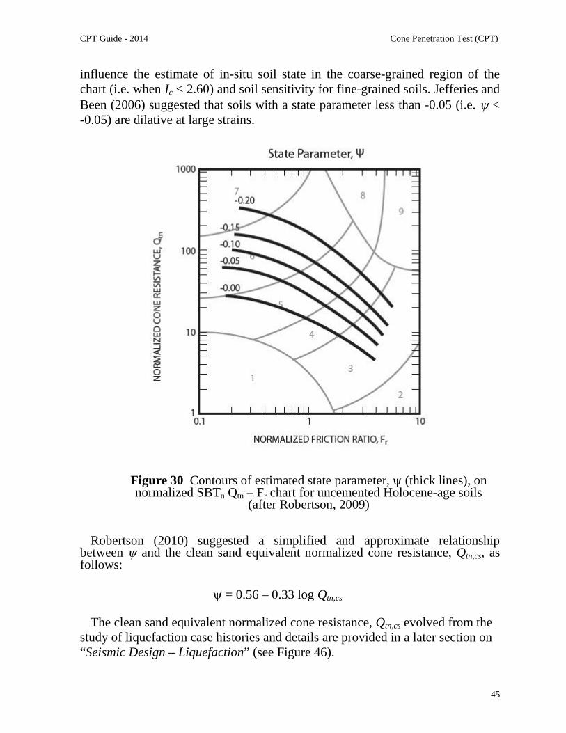
Based on the data presented by Jefferies and Been (2006) and Shuttle andCunning (2007) as well the measurements from the CANLEX project (Wride etal, 2000) for predominantly, coarse-grained uncemented young soils, combinedwith the link between OCR and state parameter in fine-grained soil, Robertson(2009) developed contours of state parameter () on the updated SBTn Qtn – Fchart for uncemented, Holocene-age soils. The contours of , that are shown onFigure 30, are approximate since stress state and plastic hardening will also
CPT Guide - 2014 Cone Penetration Test (CPT)
45
influence the estimate of in-situ soil state in the coarse-grained region of thechart (i.e. when Ic < 2.60) and soil sensitivity for fine-grained soils. Jefferies andBeen (2006) suggested that soils with a state parameter less than -0.05 (i.e. <-0.05) are dilative at large strains.
Figure 30 Contours of estimated state parameter, (thick lines), onnormalized SBTn Qtn – Fr chart for uncemented Holocene-age soils
(after Robertson, 2009)
Robertson (2010) suggested a simplified and approximate relationshipbetween and the clean sand equivalent normalized cone resistance, Qtn,cs, asfollows:
= 0.56 – 0.33 log Qtn,cs
The clean sand equivalent normalized cone resistance, Qtn,cs evolved from thestudy of liquefaction case histories and details are provided in a later section on“Seismic Design – Liquefaction” (see Figure 46).
CPT Guide - 2014 Cone Penetration Test (CPT)
46
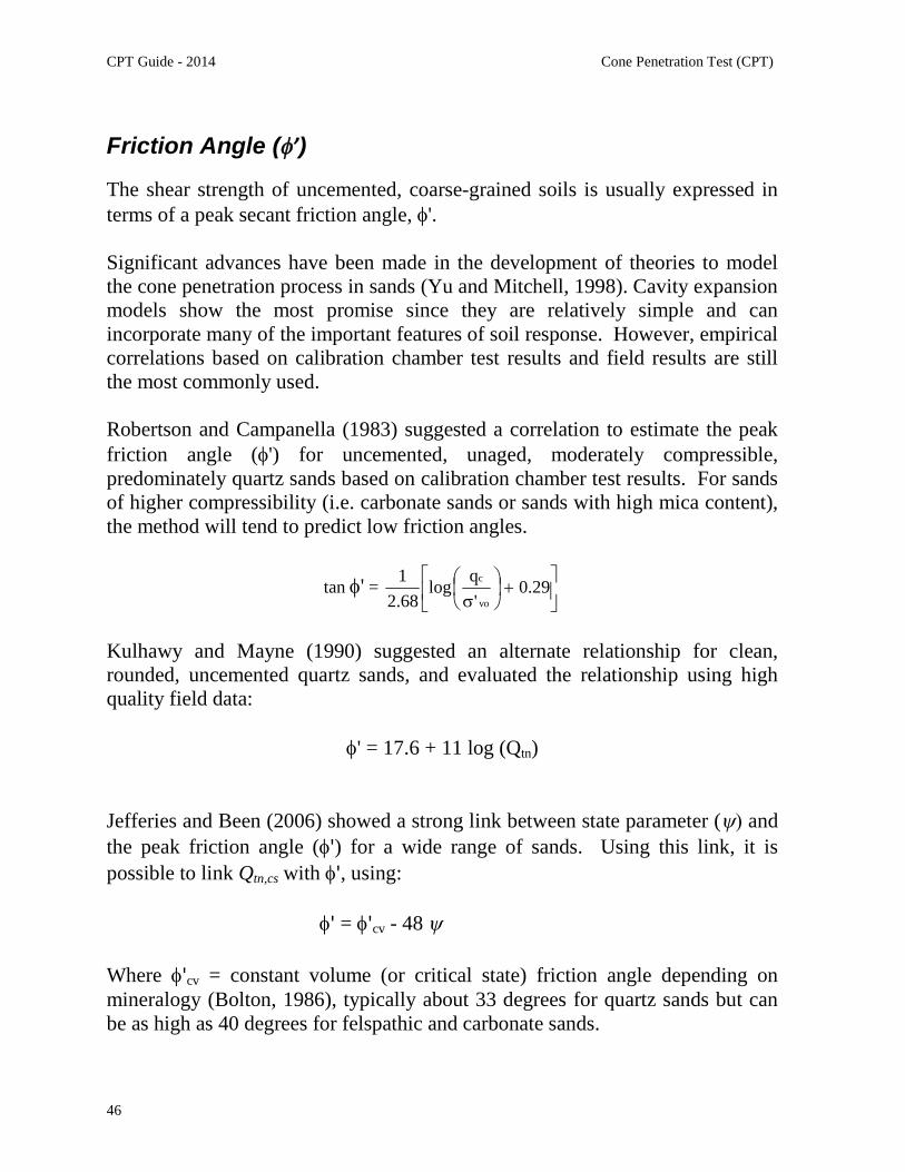
Friction Angle (’)
The shear strength of uncemented, coarse-grained soils is usually expressed interms of a peak secant friction angle, '.
Significant advances have been made in the development of theories to modelthe cone penetration process in sands (Yu and Mitchell, 1998). Cavity expansionmodels show the most promise since they are relatively simple and canincorporate many of the important features of soil response. However, empiricalcorrelations based on calibration chamber test results and field results are stillthe most commonly used.
Robertson and Campanella (1983) suggested a correlation to estimate the peakfriction angle (') for uncemented, unaged, moderately compressible,predominately quartz sands based on calibration chamber test results. For sandsof higher compressibility (i.e. carbonate sands or sands with high mica content),the method will tend to predict low friction angles.
tan ' =
29.0
'
qlog
68.2
1
vo
c
Kulhawy and Mayne (1990) suggested an alternate relationship for clean,rounded, uncemented quartz sands, and evaluated the relationship using highquality field data:
' = 17.6 + 11 log (Qtn)
Jefferies and Been (2006) showed a strong link between state parameter ( andthe peak friction angle (') for a wide range of sands. Using this link, it is
possible to link Qtn,cs with ', using:
' = 'cv - 48
Where 'cv = constant volume (or critical state) friction angle depending onmineralogy (Bolton, 1986), typically about 33 degrees for quartz sands but canbe as high as 40 degrees for felspathic and carbonate sands.

CPT Guide - 2014 Cone Penetration Test (CPT)
47
Hence, the relationship between normalized clean sand equivalent coneresistance, Qtn,cs and ' becomes:
' = 'cv + 15.84 [log Qtn,cs] – 26.88
The above relationship produces estimates of peak friction angle for clean quartzsands that are similar to those by Kulhawy and Mayne (1990). However, theabove relationship based on state parameter has the advantage that it includesthe importance of grain characteristics and mineralogy that are reflected in both'cvas well as soil type through Qtn,cs. The above relationship tends to predict 'values closer to measured values in calcareous sands where the CPT tipresistance can be low for high values of '.
For fine-grained soils, the best means for defining the effective stress peakfriction angle is from consolidated triaxial tests on high quality undisturbedsamples. An assumed value of ' = 28° for clays and 32° for silts is oftensufficient for many low-risk projects. Alternatively, an effective stress limitplasticity solution for undrained cone penetration developed at the NorwegianInstitute of Technology (NTH: Senneset et al., 1989) allows the approximateevaluation of effective stress parameters (c' and ') from piezocone (u2)measurements. In a simplified approach for normally- to lightly-overconsolidated clays and silts (c' = 0), the NTH solution can be approximatedfor the following ranges of parameters: 20º ≤ ' ≤ 40º and 0.1 ≤ Bq ≤ 1.0 (Mayne 2006):
' (deg) = 29.5º ∙Bq0.121 [0.256 + 0.336∙Bq + log Qt]
For heavily overconsolidated soils, fissured geomaterials, and highly cementedor structured clays, the above will not provide reliable results and should bedetermined by laboratory testing on high quality undisturbed samples. Theabove approach is only valid when positive (u2) pore pressures are recorded (i.e.Bq > 0.1).

CPT Guide - 2014 Cone Penetration Test (CPT)
48
Stiffness and Modulus
CPT data can be used to estimate modulus in soils for subsequent use in elasticor semi-empirical settlement prediction methods. However, correlationsbetween qc and Young’s moduli (E) are sensitive to stress and strain history,aging and soil mineralogy.
A useful guide for estimating Young's moduli for young, uncementedpredominantly silica sands is given in Figure 31. The modulus has been definedas that mobilized at about 0.1% strain. For more heavily loaded conditions (i.e.larger strain) the modulus would decrease (see “Applications” section).
Figure 31 Evaluation of drained Young's modulus (at ~ 0.1% strain) from CPTfor young, uncemented silica sands, E = E (qt - vo)
where: E = 0.015 [10 (0.55Ic + 1.68)]

CPT Guide - 2014 Cone Penetration Test (CPT)
49
Modulus from Shear Wave Velocity
A major advantage of the seismic CPT (SCPT) is the additional measurement ofthe shear wave velocity, Vs. The shear wave velocity is measured using adownhole technique during pauses in the CPT resulting in a continuous profileof Vs. Elastic theory states that the small strain shear modulus, Go can bedetermined from:
Go = Vs2
Where: is the mass density of the soil ( = /g) and Go is the small strain shearmodulus (shear strain, < 10-4 %).
Hence, the addition of shear wave velocity during the CPT provides a directmeasure of small strain soil stiffness.
The small strain shear modulus represents the elastic stiffness of the soil at shearstrains ( less than 10-4 percent. Elastic theory also states that the small strainYoung’s modulus, Eo is linked to Go, as follows;
Eo = 2(1 + )Go
where: is Poisson’s ratio, which ranges from 0.1 to 0.3 for most soils.
Application to engineering problems requires that the small strain modulus besoftened to the appropriate strain level. For most well designed structures thedegree of softening is often close to a factor of about 2.5. Hence, for manyapplications the equivalent Young’s modulus (E’) can be estimated from:
E’ ~ Go = Vs2
Further details regarding appropriate use of soil modulus for design is given inthe section on Applications of CPT Results.
The shear wave velocity can also be used directly for the evaluation ofliquefaction potential. Hence, the SCPT provides two independent methods toevaluate liquefaction potential.

CPT Guide - 2014 Cone Penetration Test (CPT)
50
Estimating Shear Wave Velocity from CPT
Shear wave velocity can be correlated to CPT cone resistance as a function ofsoil type and SBT Ic. Shear wave velocity is sensitive to age and cementation,where older deposits of the same soil have higher shear wave velocity (i.e.higher stiffness) than younger deposits. Based on SCPT data, Figure 32 shows arelationship between normalized CPT data (Qtn and Fr) and normalized shearwave velocity, Vs1, for uncemented Holocene to Pleistocene age soils, where:
Vs1 = Vs (pa / 'vo)0.25
Vs1 is in the same units as Vs (e.g. either m/s or ft/s). Younger Holocene agesoils tend to plot toward the center and lower left of the SBTn chart whereasolder Pleistocene age soil tend to plot toward the upper right part of the chart.
Figure 32 Evaluation of normalized shear wave velocity, Vs1, from CPT foruncemented Holocene and Pleistocene age soils (1m/s = 3.28 ft/sec)
Vs = [vs (qt – v)/pa]0.5 (m/s); wherevs = 10(0.55 Ic + 1.68)

CPT Guide - 2014 Cone Penetration Test (CPT)
51
Identification of soils with unusual characteristics usingthe SCPT
Almost all available empirical correlations to interpret in-situ tests assume thatthe soil is ‘well behaved’ with no microstructure, i.e. similar to soils in whichthe correlation was based. Most existing correlations apply to silica-based soilsthat are young and uncemented. Application of existing empirical correlationsin soils that are not young and uncemented can produce incorrect interpretations.Hence, it is important to be able to identify soils with ’unusual’ characteristics(i.e. microstructure). The cone resistance (qt) is a measure of large strain soilstrength and the shear wave velocity (Vs) is a measure of small strain soilstiffness (Go). Research has shown that young uncemented sands have data thatfall within a narrow range of combined qt and Go, as shown in Figure 33. Mostyoung (Holocene-age), uncemented, coarse-grained soils (Schneider and Moss,2011) have a modulus number, KG < 330, where:
KG = [Go/qt] Qtn0.75
Figure 33 Characterization of uncemented, unaged sands(modified from Eslaamizaad and Robertson, 1997)

CPT Guide - 2014 Cone Penetration Test (CPT)
52
Hydraulic Conductivity (k)
An approximate estimate of soil hydraulic conductivity or coefficient ofpermeability, k, can be made from an estimate of soil behavior type using theCPT SBT charts. Table 6 provides estimates based on the CPT-based SBTcharts shown in Figures 21 and 22. These estimates are approximate at best, butcan provide a guide to variations of possible permeability.
SBTZone
SBT Range of k(m/s)
SBTn Ic
1 Sensitive fine-grained 3x10⁻¹⁰ to 3x10⁻⁸ NA2 Organic soils - clay 1x10⁻¹⁰ to 1x10⁻⁸ Ic > 3.603 Clay 1x10⁻¹⁰ to 1x10⁻⁹ 2.95 < Ic < 3.604 Silt mixture 3x10⁻⁹ to 1x10⁻⁷ 2.60 < Ic < 2.955 Sand mixture 1x10⁻⁷ to 1x10⁻⁵ 2.05 < Ic < 2.606 Sand 1x10⁻⁵ to 1x10⁻³ 1.31 < Ic < 2.057 Dense sand to gravelly sand 1x10⁻³ to 1 Ic < 1.318 *Very dense/ stiff soil 1x10⁻⁸ to 1x10⁻³ NA9 *Very stiff fine-grained soil 1x10⁻⁹ to 1x10⁻⁷ NA
*Overconsolidated and/or cemented
Table 6 Estimated soil permeability (k) based on the CPT SBT chart byRobertson (2010) shown in Figures 21 and 22
The average relationship between soil permeability (k) and SBTn Ic, shown inTable 6, can be represented by:
When 1.0 < Ic ≤ 3.27 k = 10(0.952 – 3.04 Ic) m/s
When 3.27 < Ic < 4.0 k = 10(-4.52 – 1.37 Ic) m/s
The above relationships can be used to provide an approximate estimate of soilpermeability (k) and to show the likely variation of soil permeability with depthfrom a CPT sounding. Since the normalized CPT parameters (Qtn and Fr)respond to the mechanical behavior of the soil and depend on many soilvariables, the suggested relationship between k and Ic is approximate and shouldonly be used as a guide.

CPT Guide - 2014 Cone Penetration Test (CPT)
53
Robertson et al. (1992) presented a summary of available data to estimate thehorizontal coefficient of permeability (kh) from dissipation tests. Since therelationship is also a function of the soil stiffness, Robertson (2010) updated therelationship as shown in Figure 34.
Jamiolkowski et al. (1985) suggested a range of possible values of kh/kv for softclays as shown in Table 7.
Nature of clay kh/kv
No macrofabric, or only slightly developedmacrofabric, essentially homogeneous deposits
1 to 1.5
From fairly well- to well-developed macrofabric,e.g. sedimentary clays with discontinuous lensesand layers of more permeable material
2 to 4
Varved clays and other deposits containingembedded and more or less continuouspermeable layers
3 to 10
Table 7 Range of possible field values of kh/kv for soft clays(modified from Jamiolkowski et al., 1985)

CPT Guide - 2014 Cone Penetration Test (CPT)
54
Figure 34 Relationship between CPTu t50 (in minutes), based on u2 porepressure sensor location and 10cm2 cone, and soil permeability (kh) as a function
of normalized cone resistance, Qtn (after Robertson 2010)
CPT Guide - 2014 Cone Penetration Test (CPT)
55
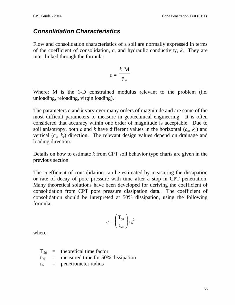
Consolidation Characteristics
Flow and consolidation characteristics of a soil are normally expressed in termsof the coefficient of consolidation, c, and hydraulic conductivity, k. They areinter-linked through the formula:
c =w
k
M
Where: M is the 1-D constrained modulus relevant to the problem (i.e.unloading, reloading, virgin loading).
The parameters c and k vary over many orders of magnitude and are some of themost difficult parameters to measure in geotechnical engineering. It is oftenconsidered that accuracy within one order of magnitude is acceptable. Due tosoil anisotropy, both c and k have different values in the horizontal (ch, kh) andvertical (cv, kv) direction. The relevant design values depend on drainage andloading direction.
Details on how to estimate k from CPT soil behavior type charts are given in theprevious section.
The coefficient of consolidation can be estimated by measuring the dissipationor rate of decay of pore pressure with time after a stop in CPT penetration.Many theoretical solutions have been developed for deriving the coefficient ofconsolidation from CPT pore pressure dissipation data. The coefficient ofconsolidation should be interpreted at 50% dissipation, using the followingformula:
c =
50
50
t
Tro
2
where:
T50 = theoretical time factort50 = measured time for 50% dissipationro = penetrometer radius

CPT Guide - 2014 Cone Penetration Test (CPT)
56
It is clear from this formula that the dissipation time is inversely proportional tothe radius of the probe. Hence, in soils of very low permeability, the time fordissipation can be decreased by using smaller diameter probes. Robertson et al.(1992) reviewed dissipation data from around the world and compared theresults with the leading theoretical solution by Teh and Houlsby (1991), asshown in Figure 35.
Figure 35 Average laboratory ch values and CPTU results(after Robertson et al., 1992, Teh and Houlsby theory shown as solid lines for Ir = 50 and 500).
The review showed that the theoretical solution provided reasonable estimates ofch. The solution and data shown in Figure 35 apply to a pore pressure sensorlocated just behind the cone tip (i.e. u2).

CPT Guide - 2014 Cone Penetration Test (CPT)
57
The ability to estimate ch from CPT dissipation results is controlled by soil stresshistory, sensitivity, anisotropy, rigidity index (relative stiffness), fabric andstructure. In overconsolidated soils, the pore pressure behind the cone tip can below or negative, resulting in dissipation data that can initially rise beforedecreasing to the equilibrium value. Care is required to ensure that thedissipation is continued to the correct equilibrium and not stopped prematurelyafter the initial rise. In these cases, the pore pressure sensor can be moved tothe face of the cone or the t50 time can be estimated using the maximum porepressure as the initial value.
Based on available experience, the CPT dissipation method should provideestimates of ch to within + or – half an order of magnitude. However, thetechnique is repeatable and provides an accurate measure of changes inconsolidation characteristics within a given soil profile.
An approximate estimate of the coefficient of consolidation in the verticaldirection can be obtained using the ratios of permeability in the horizontal andvertical direction given in the section on hydraulic conductivity, since:
cv = ch
h
v
k
k
Table 7 can be used to provide an estimate of the ratio of hydraulicconductivities.
For relatively short dissipations, the dissipation results can be plotted on asquare-root time scale. The gradient of the initial straight line is m, where;
ch = (m/MT)2 r2 (Ir)0.5
MT = 1.15 for u2 position and 10cm2 cone (i.e. r = 1.78 cm).

CPT Guide - 2014 Cone Penetration Test (CPT)
58
Constrained Modulus
Consolidation settlements can be estimated using the 1-D Constrained Modulus,M, where;
M = 1/ mv = v / e'voCc
Where mv = equivalent oedometer coefficient of compressibility.
Constrained modulus can be estimated from CPT results using the followingempirical relationship;
M = M (qt - vo)
Sangrelat (1970) suggested that M varies with soil plasticity and natural watercontent for a wide range of fine-grained soils and organic soils, although thedata were based on qc. Meigh (1987) suggested that M lies in the range 2 – 8,whereas Mayne (2001) suggested a general value of 5. Robertson (2009)suggested that M varies with Qt, such that;
When Ic > 2.2 (fine-grained soils) use:
M = Qt when Qt < 14
M = 14 when Qt > 14
When Ic < 2.2 (coarse-grained soils) use:
M = 0.0188 [10 (0.55Ic + 1.68)]
Estimates of drained 1-D constrained modulus from undrained cone penetrationwill be approximate. Estimates can be improved with additional informationabout the soil, such as plasticity index and natural water content, where M canbe lower in organic soils and soils with high water content.

CPT Guide - 2014 Cone Penetration Test (CPT)
59
Applications of CPT Results
The previous sections have described how CPT results can be used to estimategeotechnical parameters that can be used as input in analyses. An alternateapproach is to apply the in-situ test results directly to an engineering problem.A typical example of this approach is the evaluation of pile capacity directlyfrom CPT results without the need for soil parameters.
As a guide, Table 8 shows a summary of the applicability of the CPT for directdesign applications. The ratings shown in the table have been assigned based oncurrent experience and represent a qualitative evaluation of the confidence levelassessed to each design problem and general soil type. Details of groundconditions and project requirements can influence these ratings.
In the following sections a number of direct applications of CPT/CPTu resultsare described. These sections are not intended to provide full details ofgeotechnical design, since this is beyond the scope of this guide. However, theydo provide some guidelines on how the CPT can be applied to manygeotechnical engineering applications. A good reference for foundation designis the Canadian Foundation Engineering Manual (CFEM, 2007, www.bitech.ca).
Type of soil Piledesign
Bearingcapacity
Settlement* Compactioncontrol
Liquefaction
Sand 1 – 2 1 – 2 2 – 3 1 – 2 1 – 2Clay 1 – 2 1 – 2 2 – 3 3 – 4 1 – 2Intermediate soils 1 – 2 2 – 3 2 – 4 2 – 3 1 – 2
Reliability rating: 1=High; 2=High to moderate; 3=Moderate; 4=Moderate to low; 5=low* improves with SCPT data
Table 8 Perceived applicability of the CPT/CPTU for various direct designproblems

CPT Guide - 2014 Cone Penetration Test (CPT)
60
Shallow Foundation Design
General Design Principles
Typical Design Sequence:
1. Select minimum depth to protect against: external agents: e.g. frost, erosion, trees poor soil: e.g. fill, organic soils, etc.
2. Define minimum area necessary to protect against soil failure: perform bearing capacity analyses
2. Compute settlement and check if acceptable
3. Modify selected foundation if required.
Typical Shallow Foundation Problems
Study of 1200 cases of foundation problems in Europe showed that the problemscould be attributed to the following causes:
25% footings on recent fill (mainly poor engineering judgment) 20% differential settlement (50% could have been avoided with good
design) 20% effect of groundwater 10% failure in weak layer 10% nearby work (excavations, tunnels, etc.) 15% miscellaneous causes (earthquake, blasting, etc.)
In design, settlement is generally the critical issue. Bearing capacity isgenerally not of prime importance.

CPT Guide - 2014 Cone Penetration Test (CPT)
61
Construction
Construction details can significantly alter the conditions assumed in the design.
Examples are provided in the following list:
During Excavationo bottom heaveo slaking, swelling, and softening of expansive clays or rocko piping in sands and siltso remolding of silts and sensitive clayso disturbance of granular soils
Adjacent construction activityo groundwater loweringo excavationo pile drivingo blasting
Other effects during or following constructiono reversal of bottom heaveo scour, erosion and floodingo frost action

CPT Guide - 2014 Cone Penetration Test (CPT)
62
Shallow Foundation - Bearing Capacity
General Principles
Load-settlement relationships for typical footings (Vesic, 1972):
1. Approximate elastic response2. Progressive development of local shear failure3. General shear failure
In dense coarse-grained soils failure typically occurs along a well-defined failuresurface. In loose coarse-grained soils, volumetric compression dominates andpunching failures are common. Increased depth of overburden can change adense sand to behave more like loose sand. In (homogeneous) fine-grainedcohesive soils, failure occurs along an approximately circular surface.
Significant parameters are: nature of soils density and resistance of soils width and shape of footing depth of footing position of load.
A given soil does not have a unique bearing capacity; the bearing capacity is afunction of the footing shape, depth and width as well as load eccentricity.
General Bearing Capacity Theory
Initially developed by Terzaghi (1936); there are now over 30 theories with thesame general form, as follows:
Ultimate bearing capacity, (qf):
qf = 0.5 B Nsi + c Nc sc ic + D Nq sq iq
where:
N Nc Nq = bearing capacity coefficients (function of ')
sscsq = shape factors (function of B/L)

CPT Guide - 2014 Cone Penetration Test (CPT)
63
iiciq = load inclination factorsB = width of footingD = depth of footingL = length of footing
Complete rigorous solutions are impossible since stress fields are unknown. Alltheories differ in simplifying assumptions made to write the equations ofequilibrium. No single solution is correct for all cases.
Shape Factors
Shape factors are applied to account for 3-D effects. Based on limitedtheoretical ideas and some model tests, recommended factors are as follows:
sc = sq = 1 +
c
q
N
N
L
B
s = 1 - 0.4
L
B
Load Inclination Factors
When load is inclined (), the shape of a failure surface changes and reduces thearea of failure, and hence, a reduced resistance. At the limit of inclination, =, qf = 0, since slippage can occur along the footing-soil interface.
In general:
ic = iq =2
ο901
i =2
1
For an eccentric load, Terzaghi proposed a simplified concept of an equivalentfooting width, B'.
B' = B - 2 e

CPT Guide - 2014 Cone Penetration Test (CPT)
64
where ‘e’ is the eccentricity. For combined inclined and eccentric load, use B'and relevant values of shape factors. For footings near a slope, use modifiedbearing capacity factors (e.g. Bowles, 1982). They will be small for clay butlarge for granular soils.
Effect of Groundwater
The bearing capacity is based on effective stress analysis hence position of thegroundwater table affects the value of the soil unit weight.
If depth to the water table, dw = 0, use ' in both terms If dw = D (depth of footing), use ' in width term and in depth term.
In general, install drainage to keep dw > D.
Indirect Methods Based on Soil Parameters
Granular, coarse-grained soils
Bearing capacity is generally not calculated, since settlements control, except forvery narrow footings.
Cohesive, fine-grained soils
Short-term stability generally controls, hence application of undrained shearstrength, su.
qf = Nc su + Dwhere:
Nc = function of footing width and shape; for strip footings at the groundsurface, Nc = ( + 2).
su = apply Bjerrum’s correction, based on past experience, to field vane shearstrength or from CPT.
Allowable bearing capacity:
qall = (qf - D) / FS

CPT Guide - 2014 Cone Penetration Test (CPT)
65
Hence, qall =FS
N c us
Where: FS is Factor of Safety, typically = 3.0.
Use a high FS to account for limitations in theory, underestimation of loads,overestimation of soil strength, avoid local yield in soil and keep settlementssmall.
Direct Approach to estimate Bearing Capacity (In-Situ Tests)
Based on in-situ tests, theory, model tests and past foundation performance.
SPT
Empirical direct methods Limited to granular soils, however, sometimes applied to very stiff clays Often linked to allowable settlement of 25mm (Terzaghi & Peck) SPT of poor reliability, hence, empirical methods tend to be very
conservative
CPT
Empirical direct methods:
Granular, coarse-grained soils:
qf = K qc (av)
where:qc (av) = average CPT penetration resistance below depth of footing, z = B
Eslaamizaad & Robertson (1996) suggested K = 0.16 to 0.30 depending onB/D and shape. In general, assume K = 0.16 (see Figure 36). Meyerhof(1956) suggested K = 0.30. However, generally settlements will control.

CPT Guide - 2014 Cone Penetration Test (CPT)
66
Figure 36 Correlation between bearing capacity of footing on cohesionlesssoils and average cone resistance
(after Eslaamizaad and Robertson, 1996)
Cohesive, fine-grained soils:
qf = Ksu qc (av) + D
Ksu = 0.30 to 0.60 depending on footing B/D and shape and soil OCR andsensitivity. In general, assume Ksu= 0.30 in clay

CPT Guide - 2014 Cone Penetration Test (CPT)
67
Shallow Foundation Design – Settlement
General Design Principles
Requires: magnitude of settlement rate of settlement compatibility with acceptable behavior of building
For well-designed foundations, the magnitude of strains in the ground isgenerally very small ( < 10-1 %). Hence, ground response is approximatelyelastic (non-linear elastic).
Granular coarse-grained soils
Coarse-grained soils have high permeability, thus immediate settlements.However, long term settlements can occur due to submergence, change in waterlevel, blasting, machine vibration or earthquake loading.
Cohesive fine-grained soils
Fine-grained soils have very low permeability, thus the need to considermagnitude and duration of settlement.
In soft, normally to lightly overconsolidated clays, 80% to 90% of settlement isdue to primary consolidation. Secondary settlement also can be large. In stiff,overconsolidated clays (OCR > 4), approximately 50% of settlement can be dueto immediate distortion settlement and secondary settlement is generally small.
Methods for granular coarse-grained soils
Due to difficulty in sampling, most methods are based on in-situ tests, eitherdirect or via estimate of equivalent elastic modulus (E').
For most tests, the link between test result and modulus is empirical, since itdepends on many variables; e.g. mineralogy, stress history, stress state, age,cementation, etc.

CPT Guide - 2014 Cone Penetration Test (CPT)
68
CPT
Meyerhof (1974) suggested that the total settlement, s, could be calculated usingthe following formula:
s =c(av)2q
Bp
where:p = net footing pressureB = footing widthqc (av) = average CPT penetration resistance below depth of footing,z = B
Schmertmann (1970) recommended using the following equation:
s = C1 C2 p
E'C
I
3
z z
where:
C1 = correction for depth of footing= 1 – 0.5('1/p)
C2 = correction for creep and cyclic loading= 1 + 0.2 log (10 tyr)
C3 = correction for shape of footing= 1.0 for circular footings= 1.2 for square footings= 1.75 for strip footings
'1 = effective overburden pressure at footing depth (see Figure 37)p = net footing pressuretyr = time in years since load applicationIz = strain influence factor (see Figure 37)
z = thickness of sublayerE' =Equivalent Young's modulus qc = function of degree of loading, soil density, stress history, cementation,
age, grain shape and mineralogy (e.g. Figure 38)
= 2 to 4 for very young, normally consolidated sands;= 4 to 10 for aged (> 1,000years), normally consolidated sands;= 6 to 20 for overconsolidated sands
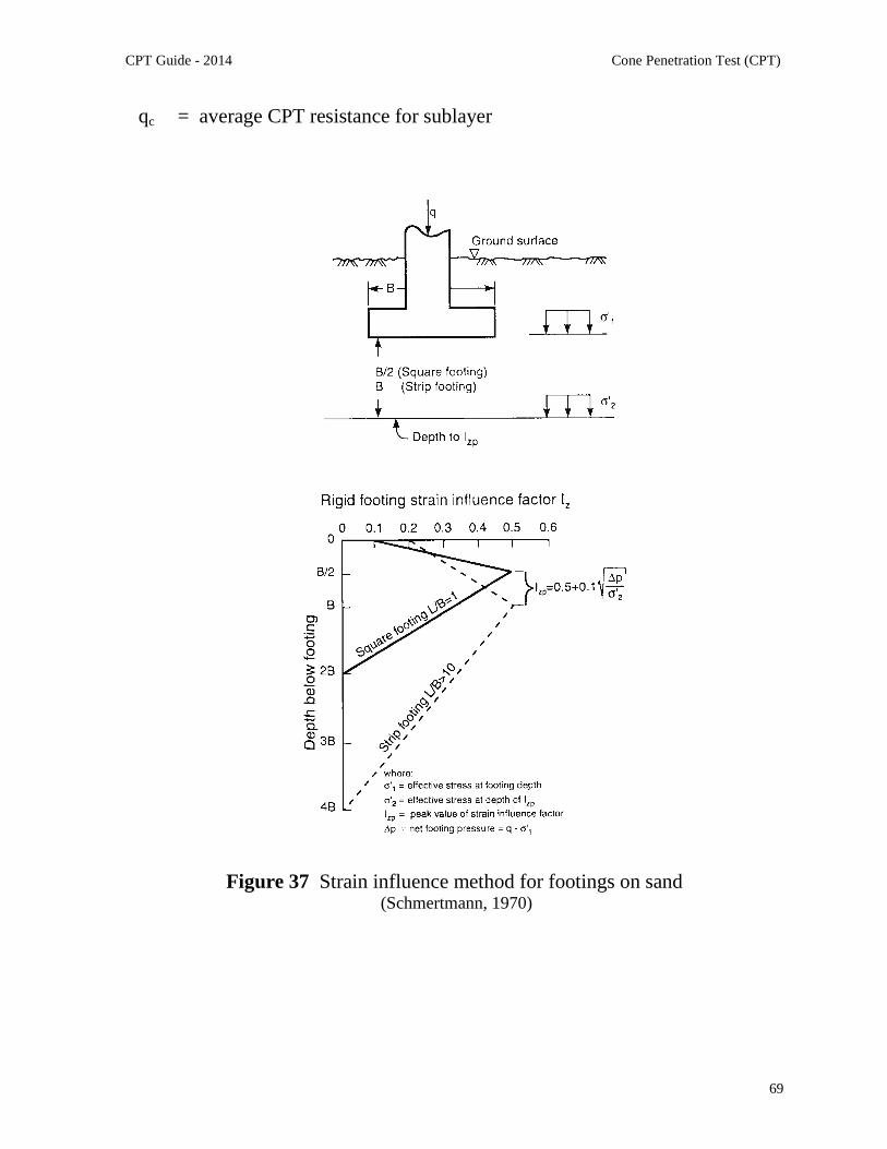
CPT Guide - 2014 Cone Penetration Test (CPT)
69
qc = average CPT resistance for sublayer
Figure 37 Strain influence method for footings on sand(Schmertmann, 1970)

CPT Guide - 2014 Cone Penetration Test (CPT)
70
Figure 38 Evaluation of drained Young's modulus from CPTfor uncemented sandy soils, E = E (qt - vo)
Where: E = 0.015 [10 (0.55Ic + 1.68)]
In this method, (see Figure 39) the sand is divided into a number of layers, n, ofthickness, z, down to a depth below the base of the footing equal to 2B for asquare footing and 4B for a strip footing (length of footing, L > 10B). A valueof qc is assigned to each layer, as illustrated in Figure 39. Note in sandy soils qc
= qt.

CPT Guide - 2014 Cone Penetration Test (CPT)
71
Figure 39 Application of Schmertmann (1970) method for settlement offootings on sand
Based on a review of 30 full-size footing tests on 12 different sands, Mayne andIllingsworth (2010) suggested the following simple relationship:
B
s
q
q
53
c
applied
where:qapplied = applied footing stressqc = average cone resistance within 1.5B below footing

CPT Guide - 2014 Cone Penetration Test (CPT)
72
Seismic Shear Wave Velocity
Eslaamizaad and Robertson (1996) suggested using shear wave velocity (Vs) tomeasure small strain stiffness (Go) directly and applying it to settlementcalculations, as follows:
Go =g
(Vs)
2
Then, the equivalent Young’s modulus can be estimated as follows:
E' = 2(1 + )Go 2.6Go
where:
= a function of the degree of loading and stress history (see Figure 40).
Fahey, (1998) suggested that the variation of could be defined by:
G/Go = 1 – f (q/qult)g
Mayne (2005) suggested that values of f = 1 and g = 0.3 are appropriate foruncemented soils that are not highly structured and these values agree well withthe NC relationship shown in Figure 40. Hence,
E' = 0.047 [1 – (q/qult)0.3] [10 (0.55Ic + 1.68)] (qt - vo)
Since settlement is a function of degree of loading, it is possible to calculate theload settlement curve, as follows:
s =
E'
Bpic
where: ic = influence coefficient

CPT Guide - 2014 Cone Penetration Test (CPT)
73
In general, for most well designed shallow foundations, q/qult = 0.3 (i.e. FS > 3),then ~ 0.3, hence, E' Go
Figure 40 Factor versus q/qult for sands with various densities and stresshistories
Shear wave velocity has the advantage of providing a direct measure of soilstiffness without an empirical correlation. The only empiricism is to adjust thesmall strain modulus for effects of stress level and strain level below the footing.The shear wave velocity approach can also be applied to estimate settlements invery stiff clays where consolidation settlements are very small.
Methods for cohesive fine-grained soils
The key parameter is the preconsolidation pressure, 'p. This can only bemeasured accurately in the laboratory on high quality samples. However, OCRand 'p profiles can be estimated from the CPT. It is useful to link results fromhigh quality laboratory tests with continuous profiles of the CPT.

CPT Guide - 2014 Cone Penetration Test (CPT)
74
In general, to keep settlements small, the applied stress must be < 'p. In softground this may require some form of ground improvement.
Components of settlement are:si = immediate (distortion) settlementsc = consolidation settlementss = secondary time dependent (creep) settlement
Immediate Settlements
Based on elastic theory, Janbu (1963) proposed:
si =
uE
Bpo 1
where:B = footing widthp = net pressureEu = soil modulus (undrained)o, 1 = influence factors for depth of footing and thickness of compressible
layer
Undrained modulus can be estimated from undrained shear strength (su) fromeither field vane tests and/or the CPT, but requires knowledge of soil plasticity.
Eu = n. su
Where: n varies from 40 to 1000, depending on degree of loading and plasticityof soil (see Figure 41).

CPT Guide - 2014 Cone Penetration Test (CPT)
75
Figure 41 Selection of soil stiffness ratio for clays(after Ladd et al., 1977)

CPT Guide - 2014 Cone Penetration Test (CPT)
76
Consolidation Settlements
Terzaghi’s 1-D theory of consolidation often applies, since 2- and 3-D effectsare generally small. Settlement for a wide range of footings and soils can becalculated using the 1-D constrained modulus, M, using:
vol = ('v / M)
Hence, s = ('v / M ) H
The 1-D Constrained Modulus (M) can be estimated from the CPT using:
M = M (qt - vo)
When Ic > 2.2 (fine-grained soils) use:
M = Qt when Qt < 14
M = 14 when Qt > 14
When Ic < 2.2 (coarse-grained soils) use:
M = 0.0188 [10 (0.55Ic + 1.68)]
The above approach can be applied to all soils, since M can be estimated for awide range of soils. The above approach is simpler than the Schmertmann(1970) approach that is limited to only sands. When using CPT results, thesettlement can be calculated over each depth increment and the total settlementbecomes the summation over the full depth. The above approach, based on 1-Dconstrained modulus, M, is often suitable for many projects. Care is requiredwhen applying the above approach to lightly overconsolidated soils if loadingwill significantly exceed 'p.

CPT Guide - 2014 Cone Penetration Test (CPT)
77
Rate of settlement is important, hence, the need for coefficient of consolidation,cv. Experience shows that cv can be highly variable due to non-linearity of thestress-strain relationship as well as change in permeability as soils compress.Values of cv can be best estimated either:
1. Separately from 1-D constrained modulus, M (or mv, since M = 1/mv)from oedometer tests on high quality samples and permeability, k from in-situ tests, using:
cv =w
Mk
or
2. Directly from CPTu dissipation tests.
cv values vary by orders of magnitude, hence, accuracy of the calculation isgenerally very poor. Drainage conditions play a major role, yet are difficult toidentify. The CPTu can provide an excellent picture of the drainage conditions.Avoid a design that depends on the time-settlement relationship. For settlementsensitive structures, try to minimize differential settlements (e.g. Osaka Airport -mechanical adjustments due to very large long term settlements).
Secondary Settlements
Time dependent settlements depend on soil mineralogy and degree of loading.Organic soils can have high secondary settlement. In general, avoid soils withhigh secondary settlements. Mesri, (1994) suggested a simplified approach that
links coefficient of secondary consolidation (C) and compression index, Cc, forinorganic clays and silts, as follows:
C = 0.04
o
c
e1
C~ 0.1 ('v /M)
Long term secondary (creep) settlement, ss is then:
ss = C z log (t/tp)
where tp is duration of primary consolidation.

CPT Guide - 2014 Cone Penetration Test (CPT)
78
Provided that the applied stress is less than 80% of 'p, secondary consolidationis generally small. Constrained Modulus, M can be estimated from the CPT (seeearlier section).
Allowable Settlements
Loads considered in settlement analyses depend on nature of soil and time-dependence of settlement. Differential settlements generally control.
Sands
Load: maximum possible load due to immediate settlementDifferential settlement: can be up to 100% of maximum settlement due to
natural variability of sand. Typically less than or equal to 25mm (1 inch)
Clays
Load: dead load plus % of live load (LL) depending on duration of live load 50% of LL for buildings 30% of LL for bridges 75% of LL for reservoirs
Settlements: are more uniform and can be larger than 25mm (1 inch)
Typical Design Sequence
1. Check for possible isolated footing design2. Check for possible raft foundation3. Ground improvement4. Deep foundations

CPT Guide - 2014 Cone Penetration Test (CPT)
79
Raft Foundations
Consider a raft when:
Area of footing > 50% of building area Need to provide underground space in location of high groundwater Need to reduce magnitude of total settlements (i.e. floating foundation) Need to reduce differential settlements
A raft is an inverted slab, designed to distribute structural loads from columnsand walls, while keeping deformations within acceptable limits.
The structural characteristics of a raft foundation can be optimized byaccounting for the interaction between the raft and supporting ground.Structural engineers usually perform an elastic analysis using elastic (Winkler)springs. Hence, they would like the spring constant, ks.
ks = coefficient of subgrade reaction (kN/m3)
ks =s
p
where:
p = net applied stresss = settlement resulting from applied stress, p
The process is governed by the relative stiffness of the structure and the ground.The coefficient of subgrade reaction is not a soil parameter, since it depends onthe size of the footing and degree of loading. Often estimates are made fromglobal tables (Terzaghi; see Table 9).

CPT Guide - 2014 Cone Penetration Test (CPT)
80
Soil type Subgrade reaction(kN/m3)
Loose sand 5,000 – 16,000Medium dense sand 10,000 – 80,000Dense sand 60,000 – 125,000Clayey sand 30,000 – 80,000Silty sand 20,000 – 50,000Clayey soil:
su < 50 kPa 10,000 – 20,00050kPa < su < 100kPa 20,000 – 50,000100 kPa < su >50,000
Table 9 Recommended coeffiecient of subgrade reaction (ks) for different soiltypes (Terzaghi, 1955)
It is best to obtain estimates based on in-situ testing.
Plate Load Tests (PLT)
Plate load tests can provide a direct measure of the relationship between p and s,but size effects can dominate results. Terzaghi (1955) suggested a link betweena 1-foot square plate (ks1) and the width of footing B, as follows:
ks = ks1
2
2B
1B
However, there is very large scatter in the results, due to variability in groundstiffness with depth.
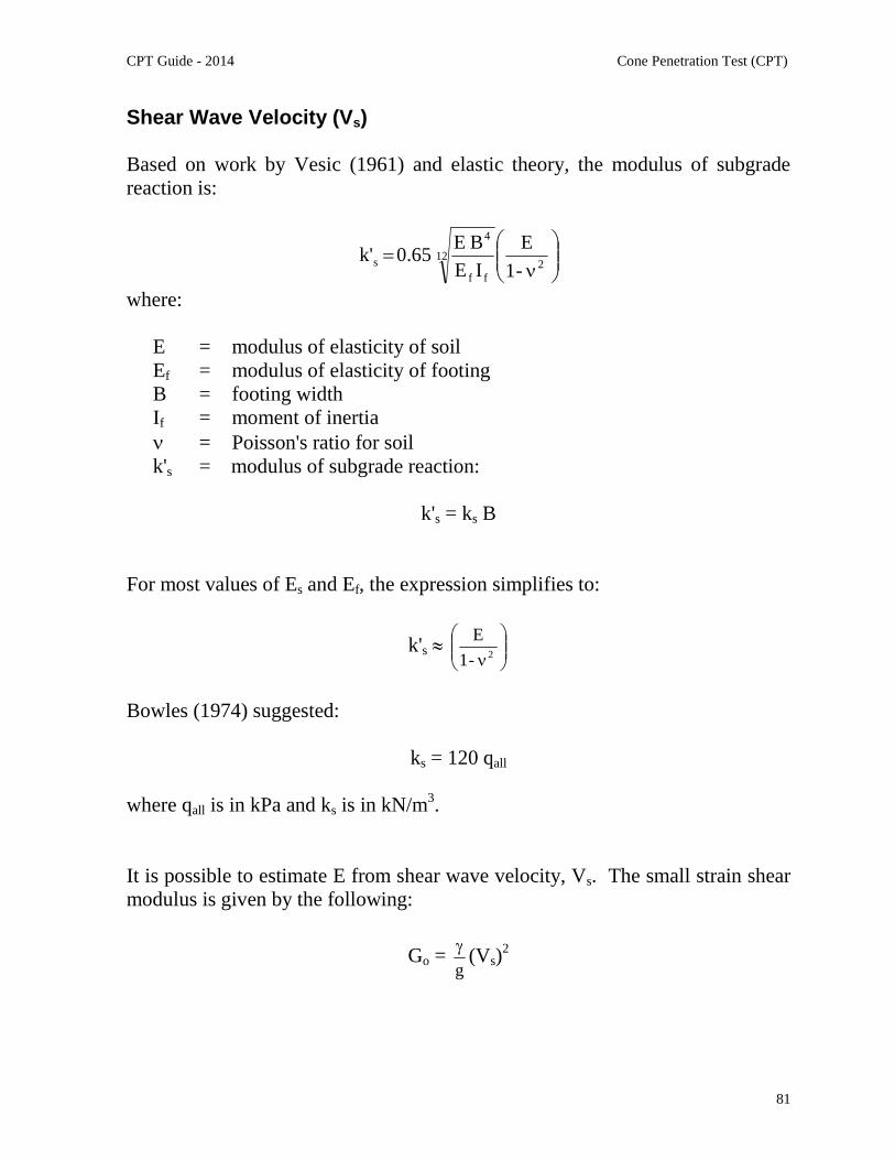
CPT Guide - 2014 Cone Penetration Test (CPT)
81
Shear Wave Velocity (Vs)
Based on work by Vesic (1961) and elastic theory, the modulus of subgradereaction is:
212
ff
4
s-1
E
IE
BE65.0k'
where:
E = modulus of elasticity of soilEf = modulus of elasticity of footingB = footing widthIf = moment of inertia = Poisson's ratio for soilk's = modulus of subgrade reaction:
k's = ks B
For most values of Es and Ef, the expression simplifies to:
k's
2-1
E
Bowles (1974) suggested:
ks = 120 qall
where qall is in kPa and ks is in kN/m3.
It is possible to estimate E from shear wave velocity, Vs. The small strain shearmodulus is given by the following:
Go =g
(Vs)
2

CPT Guide - 2014 Cone Penetration Test (CPT)
82
In addition:Geq = Go
and
E = 2(1 + ) Geq
Since 0.2 to 0.3,
k's = ks B 2.9 Go
Hence:
ks 2.9
2
s
B
Vg
where:
a function of the degree of loading and stress history (see Figure 40).
Fahey, (1998) suggested that the variation of could be defined by:
G/Go = 1 – f (q/qult)g
Mayne (2005) suggested that values of f = 1 and g = 0.3 are appropriate for mostuncemented soils that are not highly structured and these values agree well withthe NC relationship shown in Figure 40. The value of g increases toward avalue of 1.0 when the soil is overconsolidated or under increasing number ofload cycles.
For most well designed foundations, q/qult = 0.3 (i.e. FS > 3) and hence, = 0.3,then:
ks G
CPT Guide - 2014 Cone Penetration Test (CPT)
83
Deep Foundation Design
Piles
Piles can be used to:
Transfer high surface loads, through soft layers down to stronger layers Transfer loads by friction over significant length of soil Resist lateral loads Protect against scour, etc. Protect against swelling soils, etc
Piles are generally much more expensive than shallow footings.
Types of Piles
Generally classified based on installation method (Weltman & Little, 1977):
Displacement
o Preformedo Driven Cast-in-placeo High pressure grouted
Non/low-displacement
o Mud boredo Cased boredo Cast-in-place screwed (auger)o Helical (screw)
Contractors are developing new pile types and installation techniques constantlyto achieve increased capacity and improved cost effectiveness for differentground conditions. Hence, it is difficult to predict capacity and load-settlementresponse for all piles using simple analytical techniques, since the capacity andload response characteristics can be dominated by the method of installation.

CPT Guide - 2014 Cone Penetration Test (CPT)
84
Selection of Pile Type
1. Assess foundation loads2. Assess ground conditions3. Are piles necessary?4. Technical considerations:
Ground conditions Loading conditions Environmental considerations Site and equipment constraints Safety
5. List all technically feasible pile types and rank in order of suitability based ontechnical considerations
6. Assess cost of each suitable pile type and rank based on cost considerations7. Assess construction program for each suitable pile type and rank8. Make overall ranking based on technical, cost and program considerations
General Design Principles
Axial Capacity
The total ultimate pile axial capacity, Qult, consists of two components: endbearing load (or point resistance), Qb, and side friction load (sometimes referredto as the shaft or skin friction), Qs, as follows:
Qult = Qs + Qb
In sands, the end bearing, Qb, tends to dominate, whereas in soft clays, the sidefriction, Qs, tends to dominate. The end bearing, Qb, is calculated as the productbetween the pile end area, Ap, and the unit end bearing, qp. The friction load, Qs,is the product between the outer pile shaft area, As, by the unit side friction, fp.
Qult = fp As + qp Ap
Obviously, different fp values are mobilized along different parts of the pile, sothat, in practice, the calculation is performed as a summation of smallcomponents. For open-ended piles, some consideration should be made

CPT Guide - 2014 Cone Penetration Test (CPT)
85
regarding whether the pile is plugged or unplugged (de Ruiter and Beringen,1979), but the procedure is essentially as outlined above. In general, most pipepiles behave plugged (closed-ended) at working loads, but become unplugged(open-ended) at failure. The allowable or design pile load, Qall will be thengiven by the total ultimate axial capacity divided by a factor of safety.Sometimes separate factors of safety are applied to Qb and Qs.
Basic approaches are:
Static Methods Pile Dynamics Pile Load Tests
Static Methods
Pseudo-theoretical Approach
Pseudo-theoretical methods are based on shear strength parameters.
Similar to bearing capacity calculations for shallow foundations - there are over20 different bearing capacity theories. No single solution is applicable to allpiles and most cannot account for installation technique. Hence, there has beenextensive application of in-situ test techniques applied via empirical directdesign methods.
The most notable is the application of the CPT, since the CPT is a close modelof the pile process. Detailed analysis is generally limited to high-risk piledesign, such as large offshore piles.
Effective Stress Approach ()
The effective stress ( approach (Burland, 1973), has been very useful inproviding insight of pile performance.
Unit side friction, fp = v’
Unit end bearing, qp = Nt b’

CPT Guide - 2014 Cone Penetration Test (CPT)
86
Soil Type Cast-in-placePiles
DrivenPiles
Silt 0.2 - 0.3 0.3 - 0.5Loose sand 0.2 - 0.4 0.3 - 0.8Medium sand 0.3 - 0.5 0.6 - 1.0Dense sand 0.4 - 0.6 0.8 - 1.2Gravel 0.4 - 0.7 0.8 - 1.5
Table 10 Range of coefficients: cohesionless soils
Soil Type Cast-in-placePiles
DrivenPiles
Silt 10 - 30 20 - 40Loose sand 20 - 30 30 - 80Medium sand 30 - 60 50 - 120Dense sand 50 - 100 100 - 120Gravel 80 - 150 150 - 300
Table 11 Range of Nt factors: cohesionless soils
The above coefficients are approximate since they depend on groundcharacteristics and pile installation details. In the absence of pile load testsassume FS = 3.
Randolph and Wroth (1982) related to the overconsolidation ratio (OCR) forcohesive soils and produced tentative design charts. In general, for cohesivesoils:
= 0.25 - 0.32, and Nt = 3 - 10
Effective stress concepts may not radically change empirical based design rules,but can increase confidence in these rules and allow extrapolation to newsituations.

CPT Guide - 2014 Cone Penetration Test (CPT)
87
Total Stress Approach ()
It has been common to design piles in cohesive soils based on total stress andundrained shear strength, su.
Unit side friction, fp = su
Unit end bearing, qp = Nt su
Where varies from 0.5 - 1.0 depending on OCR and Nt varies from 6 to 9depending on depth of embedment and pile size.
Empirical Approach
CPT Method
Research has shown (Robertson et al., 1988; Briaud and Tucker, 1988; Tand andFunegard, 1989; Sharp et al., 1988) that CPT methods generally give superiorpredictions of axial pile capacity compared to most conventional methods. Themain reason for this is that the CPT provides a continuous profile of soilresponse. Almost all CPT methods use reduction factors to measured CPTvalues. The need for such reduction factors is due to a combination of thefollowing influences: scale effect, rate of loading effects, difference of insertiontechnique, position of the CPT friction sleeve and differences in horizontal soildisplacements. The early work by DeBeer (1963) identified the importance ofscale effects. Despite these differences, the CPT is still the test that gives theclosest simulation of a pile. Superiority of CPT methods over non-CPT methodshas been confirmed in other studies (e.g. O'Neill, 1986).
The main CPT method by Bustamante and Gianeselli (1982 - LCPC Method) isoutlined below. The LCPC CPT method is recommended since it providessimple guidance to account for many different pile installation methods andgenerally provides good estimates of axial capacity of single piles.

CPT Guide - 2014 Cone Penetration Test (CPT)
88
LCPC CPT Method (Bustamante and Gianeselli, 1982)
The method by Bustamante and Gianeselli was based on the analysis of 197 pileload (and extraction) tests with a wide range of pile and soil types, which maypartly explain the good results obtained with the method. The method, alsoknown as the LCPC method, is summarized in Table 12 and Table 13. TheLCPC method was updated with small changes by Bustamante and Frank,(1997)
Table 12 Bearing capacity factors, kc
(Bustamante and Gianeselli, 1982)
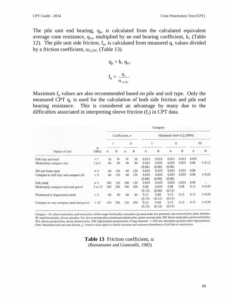
CPT Guide - 2014 Cone Penetration Test (CPT)
89
The pile unit end bearing, qp, is calculated from the calculated equivalentaverage cone resistance, qca, multiplied by an end bearing coefficient, kc (Table12). The pile unit side friction, fp, is calculated from measured qc values dividedby a friction coefficient, LCPC (Table 13).
qp = kc qca
fp =LCPC
cq
Maximum fp values are also recommended based on pile and soil type. Only themeasured CPT qc is used for the calculation of both side friction and pile endbearing resistance. This is considered an advantage by many due to thedifficulties associated in interpreting sleeve friction (fs) in CPT data.
Table 13 Friction coefficient, (Bustamante and Gianeselli, 1982)

CPT Guide - 2014 Cone Penetration Test (CPT)
90
The equivalent average cone resistance, qca, at the base of the pile used tocompute the pile unit end bearing, qp, is the mean qc value measured along twofixed distances, a, (a = 1.5D, where D is the pile diameter) above (-a) and below(+a) the pile tip. The authors suggest that qca be calculated in three steps, asshown in Figure 42. The first step is to calculate q'ca, the mean qc between -aand +a. The second step is to eliminate values higher than 1.3q'ca along thelength -a to +a, and the values lower than 0.7q'ca along the length -a, whichgenerates the thick curve shown in Figure 42. The third step is to calculate qca,the mean value of the thick curve.
Figure 42 Calculation of equivalent average cone resistance(Bustamante and Gianeselli, 1982).
Other Design Considerations
Factor of Safety
In order to obtain the design load, factors of safety are applied to the ultimateload and a deterministic approach is usually adopted to define these values. Theselection of an appropriate factor of safety depends on many factors, such as

CPT Guide - 2014 Cone Penetration Test (CPT)
91
reliability and sufficiency of the site investigation data, confidence in themethod of calculation, previous experience with similar piles in similar soils andwhether or not pile load test results are available.
Factors of safety are generally of the order of 2, although real values aresometimes greater, as partial factors of safety are sometimes applied duringcalculations (particularly to soil strengths) before arriving to the ultimate pilecapacity.
Recommended factors of safety for calculating the axial capacity of piles fromthe CPT are given in Table 14.
Method Factor of safety (FS)
Bustamante andGianeselli (1982)
2.0 (Qs)3.0 (Qb)
de Ruiter and Beringen(1979)
2.0 (static loads)1.5 (static + storm loads)
Table 14 Recommended factors of safety for axial capacity of piles from CPT
The design of high capacity large diameter bored piles in stiff clay or dense sandcan be difficult due to the fact that settlement criteria usually control rather thancapacity. Hence, very high factors of safety are often applied to limit settlement.
Pile Dynamics
The objective of methods that rely on pile dynamics is to relate the dynamic pilebehavior to the ultimate static pile resistance. Hence, pile dynamics can workwell in drained soils (sands, gravels, etc.) but can be difficult in undrained soils(silts, clays, etc.).
The early approach was to use simple pile driving equations (Hiley, EngineeringNews, etc.) based on equating the available energy of the hammer to the workperformed by the pile. However, these were based on a rigid pile concept,which is fundamentally incorrect. Current approaches are based on 1-D wave-equation analyses (Goble et al., 1970). This method takes into account the

CPT Guide - 2014 Cone Penetration Test (CPT)
92
characteristics of the hammer, driving cap, pile and soil. The method iscommonly applied using commercial software (i.e. WEAP). This method isgood to assist in selection of hammers and prediction of driving stresses and thechoice of driving criteria. It is also useful for dynamic monitoring duringconstruction.
Pile Load Tests
Since there is much uncertainty in the prediction of pile capacity and response, itis common to perform pile load tests on major projects.
For major projects, it is common to apply static methods (i.e. LCPC CPTmethod) to obtain a first estimate of capacity, apply pile dynamics if driven pilesselected (aid in hammer selection, driving stresses, driving criteria) and performa small number of pile load tests to evaluate pile response and to calibrate thestatic method. Results from the pile load tests can be used to modify the staticprediction (i.e. CPT prediction) of pile capacity and the modified methodapplied across the site. For low-risk projects, pile load tests may not bewarranted and a slightly conservative prediction should be applied using thestatic (CPT) method.
Group Capacity
The capacity of a group of piles is influenced by the spacing, pile installationand ground conditions. The group efficiency is defined as the ratio of the groupcapacity to the sum of the individual pile capacities.
Driven piles in coarse-grained soils develop larger individual capacities wheninstalled as a group since lateral earth pressures and soil density increase due topile driving. Hence, it is conservative to use the sum of the individual pilecapacities.
For bored pile groups, the individual capacity can reduce due to reduced lateralstresses. Meyerhof (1976) suggested a reduction factor of 0.67.
For piles in fine-grained soils the capacity of the pile group should be estimatedbased on the ‘block’ of piles since the soil between the piles may move with thepile group.

CPT Guide - 2014 Cone Penetration Test (CPT)
93
Design of Piles in Rock
Piles can be placed on or socketed into rock to carry high loads. The exact areaof contact with rock, depth of penetration into rock and quality of rock arelargely unknown, hence, there is much uncertainty. The capacity is oftenconfirmed based on driving or installation details, local experience and testloading. End bearing capacity can be based on pressuremeter test results orstrength from rock cores. Shaft resistance should be estimated with caution, dueto possible poor contact between rock and pile, possible stress concentration andresulting progressive failure.
Pile Settlement
Although the installation of piles changes the deformation and compressibilitycharacteristics of the soil mass governing the behavior of single piles under load,this influence usually extends only a few pile diameters below the pile base.Meyerhof (1976) suggested that the total settlement of a group of piles atworking load can generally be estimated assuming an equivalent foundation.For a group of predominately friction piles (i.e. Qs > Qb), the equivalentfoundation is assumed to act on the soil at an effective depth of 2/3 of the pileembedment. For a group of piles that are predominately end bearing (i.e. Qb >Qs), the equivalent foundation is taken at or close to the base of the piles. Theresulting settlement is calculated in a manner similar to that of shallowfoundations.
Sometimes large capacity piles are installed and used as single piles and the loadsettlement response of a single pile is required. The load settlement response ofa single pile is controlled by the combined behavior of the side resistance (Qs)and base resistance (Qb). The side resistance is usually developed at a smallsettlement of about 0.5 percent of the shaft diameter and generally between 5 to10mm. In contrast to the side resistance, the base resistance requires muchlarger movements to develop fully, usually about 10 to 20 percent of the basediameter. An estimate of the load settlement response of a single pile can bemade by combining the two components of resistance according to the aboveguidelines. In this way, a friction pile (i.e. Qs >> Qb), will show a clear plungingfailure at a small settlement of about 0.5% of the pile diameter. On the otherhand, an end bearing pile (i.e. Qb >> Qs), will not show a clear plunging failure

CPT Guide - 2014 Cone Penetration Test (CPT)
94
until very large settlements have taken place and usually settlement criteriacontrol before failure can occur. In both cases, the side friction is almost fullymobilized at working loads. Hence, it is often important to correctly define theproportions of resistance (Qb/Qs).
Methods have been developed to estimate the load-transfer (t-z) curves(Verbrugge, 1988). However, these methods are approximate at best and arestrongly influenced by pile installation and soil type. The recommended methodfor estimating load settlement response for single piles is to follow the generalguidelines above regarding the development of each component of resistance.
Negative Shaft Friction and Down Drag on Piles
When the ground around a pile settles, the resulting downward movement caninduce downward forces on the pile.
The magnitude of the settlement can be very small to develop these downwardforces. For end bearing piles, the negative shaft friction plus the dead load canresult in structural failure of the pile. For friction piles, the negative shaftfriction can result in greater settlements. No pile subject to down drag will settlemore than the surrounding ground.
Lateral Response of Piles
Vertical piles can resist lateral loads by deflecting and mobilizing resistance inthe surrounding ground. The response depends on the relative stiffness of thepile and the ground. In general, the response is controlled by the stiffness of theground near the surface, since most long piles are relatively flexible.
A common approach is to simulate the ground by a series of horizontal springs.The spring stiffness can be estimated based on a simple subgrade modulusapproach (assumes the ground to be linear and homogeneous) or as non-linearsprings (p-y curves) (Matlock, 1970). The p-y curves can be estimated usingempirical relationships based on lab results or in-situ tests (e.g. pressuremeter,DMT, SCPT) (Baguelin et al., 1978; Robertson et al., 1986). The initialstiffness of the p-y curves is controlled by the small strain stiffness (Go) that canbe determined by measuring (or estimating) the shear wave velocity (Vs) usingthe SCPT.

CPT Guide - 2014 Cone Penetration Test (CPT)
95
Another approach is to simulate the ground as an elastic continuum. Poulos andDavis, (1980) and Randolph, (1981) suggested design charts that requireestimates of equivalent ground modulus for uniform homogeneous groundprofiles.
The above approaches apply to single piles. When piles are installed in groups,interaction occurs and lateral deformations can increase. These can be estimatedusing simplified theoretical solutions (Poulos and Davis, 1980, Randolph, 1981).The direction of the applied load relative to the group is important for laterallyloaded pile groups.

CPT Guide - 2014 Cone Penetration Test (CPT)
96
Seismic Design - Liquefaction(see Robertson & Wride, 1998; Zhang et al., 2002 & 2004; Robertson, 2009 for details)
Soil liquefaction is a major concern for structures constructed with or on sand orsandy soils. The major earthquakes of Niigata (1964), Kobe (1995) andChristchurch (2010/11) have illustrated the significance and extent of damagecaused by soil liquefaction. Soil liquefaction is also a major design problem forlarge sand structures such as mine tailings impoundment and earth dams.
To evaluate the potential for soil liquefaction, it is important to determine thesoil stratigraphy and in-situ state of the deposits. The CPT is an ideal in-situ testto evaluate the potential for soil liquefaction because of its repeatability,reliability, continuous data and cost effectiveness. This section presents asummary of the application of the CPT to evaluate soil liquefaction. Full detailsare contained in a report prepared for NCEER (Youd et al., 2001) as a result ofworkshops on liquefaction held in 1996/97 and in a paper by Robertson andWride (1998) and updated by Robertson (2009).
Liquefaction Definitions
Several phenomena are described as soil liquefaction, hence, the followingdefinitions are provided to aid in the understanding of the phenomena.
Flow (static) Liquefaction
Applies to strain softening soils only (i.e. susceptible to strength loss). Requires a strain softening response in undrained loading resulting in
approximately constant shear stress and effective stress. Requires in-situ shear stresses to be greater than the residual or
minimum undrained shear strength. Either static or cyclic loading can trigger flow liquefaction. For failure of a soil structure to occur, such as a slope, a sufficient
volume of material must strain soften. The resulting failure can be aslide or a flow depending on the material characteristics and groundgeometry. The resulting movements are due to internal causes andoften occur after the trigger mechanism.

CPT Guide - 2014 Cone Penetration Test (CPT)
97
Can occur in any strain-softening saturated (or near-saturated) soil,such as very loose coarse-grained (sand) deposits, very sensitive fine-grained (clay), and loose loess (silt) deposits.
Cyclic (softening) Liquefaction
Requires undrained cyclic loading during which shear stress reversaloccurs or zero shear stress can develop.
Requires sufficient undrained cyclic loading to allow effective stressesto essentially reach zero.
Deformations during cyclic loading can accumulate to large values,but generally stabilize shortly after cyclic loading stops. The resultingmovements are due to external causes and occur mainly during thecyclic loading.
Can occur in almost all saturated coarse-grained soil (sand) providedthat the cyclic loading is sufficiently large in magnitude and duration.
Fine-grained (clay) soils can experience cyclic softening when theapplied cyclic shear stress is close to the undrained shear strength.Deformations are generally small due to the cohesive strength at loweffective stress. Rate effects (creep) often control deformations incohesive soils.
Note that strain softening soils can also experience cyclic liquefaction dependingon ground geometry. Figure 43 presents a flow chart to clarify the phenomenaof soil liquefaction.

CPT Guide - 2014 Cone Penetration Test (CPT)
98
Figure 43 Flow chart to evaluate liquefaction of soils(after Robertson and Wride, 1998)
If a soil is strain softening (i.e. can experience strength loss), flow liquefaction ispossible if the soil can be triggered to strain-soften and if the gravitational shearstresses are larger than the minimum undrained shear strength. The trigger canbe either monotonic or cyclic. Whether a slope or soil structure will fail andslide will depend on the amount of strain softening soil relative to strainhardening soil within the structure, the brittleness of the strain softening soil andthe geometry of the ground. The resulting deformations of a soil structure withboth strain softening and strain hardening soils will depend on many factors,such as distribution of soils, ground geometry, amount and type of triggermechanism, brittleness of the strain softening soil and drainage conditions.Examples of flow liquefaction failures are the Aberfan flow slide (Bishop,1973), Zealand submarine flow slides (Koppejan et al., 1948) and the Stavatailings dam failure. In general, flow liquefaction failures are not common,however, when they occur, they typically take place rapidly with little warningand are usually catastrophic. Hence, the design against flow liquefaction shouldbe carried out cautiously.

CPT Guide - 2014 Cone Penetration Test (CPT)
99
If a soil is strain hardening, flow liquefaction will not occur. However, cyclic(softening) liquefaction can occur due to cyclic undrained loading. The amountand extent of deformations during cyclic loading will depend on the state(density/OCR) of the soils, the magnitude and duration of the cyclic loading andthe extent to which shear stress reversal occurs. If extensive shear stressreversal occurs and the magnitude and duration of cyclic loading are sufficientlylarge, it is possible for the effective stresses to essentially reach zero in sand-likesoils resulting in large deformations. Examples of cyclic liquefaction werecommon in the major earthquakes in Niigata (1964) and Christchurch (2010/11)and manifest in the form of sand boils, damaged lifelines (pipelines, etc.) lateralspreads, slumping of embankments, ground settlements, and ground surfacecracks.
If cyclic liquefaction occurs and drainage paths are restricted due to overlyingless permeable layers, the sand immediately beneath the less permeable soil canbecome looser due to pore water redistribution, resulting in possible subsequentflow liquefaction, given the right geometry. In cases where drainage isrestricted, caution is required to allow for possible void redistribution.
CPT for Cyclic Liquefaction – Level Ground Sites(see Robertson & Wride, 1998; Zhang et al., 2002 & 2004; Robertson, 2009 for details)
Most of the existing work on cyclic liquefaction has been primarily forearthquakes. The late Prof. H.B. Seed and his co-workers developed acomprehensive methodology to estimate the potential for cyclic liquefaction forlevel ground sites due to earthquake loading. The methodology requires anestimate of the cyclic stress ratio (CSR) profile caused by the design earthquakeand the cyclic resistance ratio (CRR) of the ground. If the CSR is greater thanthe CRR cyclic liquefaction can occur. The CSR is usually estimated based on aprobability of occurrence for a given earthquake. A site-specific seismicityanalysis can be carried out to determine the design CSR profile with depth. Asimplified method to estimate CSR was also developed by Seed and Idriss(1971) based on the peak ground surface acceleration (amax) at the site. Thesimplified approach can be summarized as follows:
CSR = dvo
vomax
vo
av r'g
a65.0
'

CPT Guide - 2014 Cone Penetration Test (CPT)
100
where av is the average cyclic shear stress; amax is the maximum horizontalacceleration at the ground surface; g is the acceleration due to gravity; vo and'vo are the total and effective vertical overburden stresses, respectively, and rd isa stress reduction factor which is dependent on depth. The factor rd can beestimating using the following tri-linear function, which provides a good fit tothe average of the suggested range in rd originally proposed by Seed and Idriss(1971):
rd = 1.0 – 0.00765zif z < 9.15 m
= 1.174 – 0.0267zif z = 9.15 to 23 m
= 0.744 – 0.008zif z = 23 to 30 m
= 0.5if z > 30 m
Where z is the depth in meters. These formulae are approximate at best andrepresent only average values since rd shows considerable variation with depth.Recently Idriss and Boulanger (2008) suggested alternate values for rd, but theseare associated with alternate values of CRR.
The sequence to evaluate cyclic liquefaction for level ground sites is:
1. Evaluate susceptibility to cyclic liquefaction2. Evaluate triggering of cyclic liquefaction3. Evaluate post-earthquake deformations.
1. Evaluate Susceptibility to Cyclic Liquefaction
The response of soil to seismic loading varies with soil type and state (voidratio, effective confining stress, stress history, etc.). Boulanger and Idriss (2004)correctly distinguished between sand-like and clay-like behavior. The followingcriteria can be used to identify soil behavior:

CPT Guide - 2014 Cone Penetration Test (CPT)
101
Sand-like Behavior: Sand-like soils are susceptible to cyclic liquefaction whentheir behavior is typically characterized by Plasticity Index (PI) < 10 and LiquidLimit (LL) < 37 and natural water content (wc) > 0.85 (LL). More emphasisshould be placed on PI, since both LL and wc tend to be less reliable.
Low risk projects: Assume soils are susceptible to cyclic liquefactionbased on above criteria unless previous local experience showsotherwise.
High risk projects: Either assume soils are susceptible to cyclicliquefaction or obtain high quality samples and evaluate susceptibilitybased on appropriate laboratory testing, unless previous localexperience exists.
Clay-like Behavior: Clay-like soils are generally not susceptible to cyclicliquefaction when their behavior is characterized by PI > 15 but they canexperience cyclic softening.
Low risk projects: Assume soils are not susceptible to cyclicliquefaction based on above criteria unless previous local experienceshows otherwise. Check for cyclic softening.
High risk projects: Obtain high quality samples and evaluatesusceptibility to either cyclic liquefaction and/or cyclic softening basedon appropriate laboratory testing, unless previous local experienceexists.
Figure 44 shows the criteria suggested by Bray and Sancio (2006) that includesa transition from sand-like to clay-like behavior between 12 < PI < 18.
Figure 44 Liquefaction susceptibility criteria (after Bray and Sancio, 2006)

CPT Guide - 2014 Cone Penetration Test (CPT)
102
These criteria are generally conservative. Boulanger and Idriss (2004)suggested that sand-like behavior is limited to PI < 7. Use the criteria shown inFigure 44, unless local experience in the same geology unit shows that a lowerPI is more appropriate.
Fine-grained soils transition from a behavior that is more fundamentally likesands to behavior that is more fundamentally like clays over a range ofAtterberg Limits and moisture contents, as shown in Figure 44. The transitionfrom more sand-like to more clay-like behavior has a direct correspondence tothe types of engineering procedures that are best suited to evaluate their seismicbehavior. The transition from sand-like to clay-like behavior generally occurswhen the SBTn 2.5 < Ic < 2.7, as illustrated in Figures 26 & 49. For soils thatplot in or close to this transition region samples should be obtained to verifybehavior.
2. Evaluate Triggering of Cyclic Liquefaction
Sand-like MaterialsSeed et al., (1985) developed a method to estimate the cyclic resistance ratio(CRR) for clean sand with level ground conditions based on the StandardPenetration Test (SPT). The CPT has become more popular to estimate CRR,due to the continuous, reliable and repeatable nature of the data (Youd et al.,2001; Robertson, 2009) and a larger database.
Apply the simplified (NCEER) approach as described by Youd et al (2001)using generally conservative assumptions. The simplified approach should beused for low- to medium-risk projects and for preliminary screening for high-risk projects. For low-risk projects, where the simplified approach is the onlymethod applied, conservative criteria should be used. The recommended CPTcorrelation for sand-like soils is shown in Figure 45 and can be estimated usingthe following simplified equations suggested by Robertson and Wride, (1998):
CRR7.5 =
08.01000
93
3
,
cstnQ
if 50 Qtn,cs 160
CRR7.5 =
05.01000
833.0,
cstnQ
if Qtn,cs < 50

CPT Guide - 2014 Cone Penetration Test (CPT)
103
The field observations, used to compile the curve in Figure 45, were basedprimarily on the following conditions:
Holocene-age, uncemented silica-based sand deposits with Ko < 0.7 Level or gently sloping ground Cyclic stress ratio (CSR)7.5 adjusted to magnitude M = 7.5 earthquake Depth range from 1 to 15 m (3 to 50 ft), 85% for depths < 10 m (30 ft) Earthquakes with magnitude mostly between 6 < M < 8 Representative average CPT values for the layer considered to have
experienced cyclic liquefaction.
Caution should be exercised when extrapolating the CPT correlation toconditions outside the above range. An important feature to recognize is that thecorrelation is based primarily on average values for the inferred liquefied layers.However, the correlation is often applied to all measured CPT values, whichinclude low values below the average. Therefore, the correlation can beconservative in variable deposits where a small part of the CPT data can indicatepossible liquefaction.
Figure 45 Cyclic resistance ratio (CRR7.5) from CPT normalized clean sandequivalent cone resistance (Qtn,cs)
(updated by Robertson, 2009)

CPT Guide - 2014 Cone Penetration Test (CPT)
104
It has been recognized for some time that the correlation to estimate CRR7.5 forsilty sands is different than that for clean sands. Typically a correction is madeto determine an equivalent clean sand penetration resistance based on graincharacteristics, such as fines content, although the corrections are due to morethan just fines content and are influenced by the plasticity of the fines.
One reason for the continued use of the SPT has been the need to obtain a soilsample to determine the fines content of the soil. However, this has been offsetby the generally poor repeatability of the SPT data. It is now possible toestimate behavior characteristics directly from the CPT. Robertson and Wride(R&W, 1998) suggest estimating an equivalent clean sand cone penetrationresistance, (Qtn)cs using the following:
(Qtn)cs = Kc Qtn
Where Kc is a correction factor that is a function of behavior characteristics (e.g.combined influence of fines content and plasticity) of the soil.
Robertson and Wride (R&W, 1998) suggest estimating behavior characteristicsusing the normalized soil behavior chart (SBTn) by Robertson (1990) and thesoil behavior type index, Ic, where:
Ic = 5.02222.1loglog47.3 FQtn
and Qtn =n
vo
a
a
vot P
P
q
'2
Qtn is the normalized CPT penetration resistance (dimensionless); n = stressexponent; F = fs/[(qc - vo)] x 100% is the normalized friction ratio (in percent);fs is the CPT sleeve friction stress; vo and 'vo are the total effective overburdenstresses respectively; Pa is a reference pressure in the same units as 'vo (i.e. Pa =100 kPa if 'vo is in kPa) and Pa2 is a reference pressure in the same units as qc
and vo (i.e. Pa2 = 0.1 MPa if qc and vo are in MPa). Note, 1 tsf ~ 0.1 MPa.
The soil behavior type chart by Robertson (1990) used a normalized conepenetration resistance (Qt) based on a simple linear stress exponent of n = 1.0,whereas the recommended chart for estimating CRR7.5 is based on a normalizedcone penetration resistance (Qtn) based on a variable stress exponent. Robertson

CPT Guide - 2014 Cone Penetration Test (CPT)
105
(2009) recently updated the stress normalization to allow for a variation of thestress exponent with both SBTn Ic and effective overburden stress using:
n = 0.381 (Ic) + 0.05 ('vo/pa) – 0.15
where n ≤ 1.0 (see Figure 46 for flow chart).
The recommended relationship between Ic and the correction factor Kc is givenby the following:
Kc = 1.0 if Ic 1.64
Kc = 5.581 Ic3 - 0.403 Ic
4 – 21.63 Ic2 + 33.75 Ic – 17.88 if Ic > 1.64
The correction factor, Kc, is approximate since the CPT responds to manyfactors such as soil plasticity, fines content, mineralogy, soil sensitivity, age, andstress history. However, in general, these same factors influence the CRR7.5 in asimilar manner. Caution should be used when applying the relationship to sandsthat plot in the region defined by 1.64 < Ic < 2.36 and F < 0.5% so as not toconfuse very loose clean sands with sands containing fines. In this zone, it issuggested to set Kc = 1.0. Soils that fall into the (dilative) clay-like region of theCPT soil behavior chart (e.g. region FD, Figure 49), in general, are notsusceptible to cyclic liquefaction. However, samples should be obtained andliquefaction potential evaluated using other criteria based primarily on plasticity,e.g. soils with plasticity index greater than about 10 are likely not susceptible toliquefaction. Soils that fall in the lower left region of the CPT soil behaviorchart defined by region FC (see Figure 49) can be sensitive and hence, possiblysusceptible to both cyclic and flow liquefaction. The full methodology toestimate CRR7.5 from the CPT is summarized in Figure 46.
For low-risk projects and for preliminary screening in high-risk projects,Robertson and Wride (1998) suggested that soils in region FC and FD (Figure49) would have clay-like behavior and would likely not be susceptible to cyclicliquefaction. Youd et al (2001) recommends that soils be sampled where Ic >2.4 to verify the behavior type. When Ic > 2.4 selected (disturbed) soil samples(for grain size distribution, Atterberg limits and water content) should beobtained and tested to confirm susceptibility to cyclic liquefaction using thecriteria in Figure 44. Selective soil sampling based on Ic should be carried outadjacent to some CPT soundings. Disturbed samples can be obtained using

CPT Guide - 2014 Cone Penetration Test (CPT)
106
either direct push samplers (e.g. Figure 1) or conventional drilling/samplingtechniques close to the CPT sounding.
The factor of safely against cyclic liquefaction is defined as:
Factor of Safety, FS =CSR
CRR 5.7 MSF
Where MSF is the Magnitude Scaling Factor to convert the CRR7.5 for M = 7.5to the equivalent CRR for the design earthquake.
The NCEER recommended MSF is given by:
MSF =56.2M
174
The above recommendations are based on the NCEER Workshops in 1996/97(Youd et al., 2001) and updated by Robertson (2009).
Juang et al., (2006) and Ku et al (2012) related Factor of Safety (FS) to theprobability of liquefaction (PL) for the R&W CPT-based method using:
PL = 1 / (1 + (FS/0.9)6.3)
CRR7.5 can also be estimated using normalized shear wave velocity Vs1 (Kayenet al, 2013). The combined application of both CPT and shear wave velocity toevaluate the potential for soil liquefaction is very useful and can beaccomplished in a cost effective manner using the seismic CPT (SCPT).
The CPT provides near continuous profiles of cone resistance that capture thefull detail of soil variability, but large corrections are required based on soiltype. The shear wave velocity is typically measured over a larger depthincrement (typically every 1m) and hence provides a more averaged measure butrequires smaller corrections for soil type. If the two approaches provide similarresults, in terms of CRR7.5, there is more confidence in the results. If the twoapproaches provide different results, further investigation can be warranted toidentify the cause (such as soil aging, cementation, etc.). Sometimes shear wavevelocities may predict a higher CRR7.5 due to slight soil bonding. In this case,the degree of bonding should be studied to determine if the earthquake loadingis sufficient to break the bonds.

CPT Guide - 2014 Cone Penetration Test (CPT)
107
Stratigraphy – transition zones
Robertson and Campanella (1983) showed that the cone tip resistance isinfluenced by the soil ahead and behind the cone tip. In strong/stiff soils thezone of influence is large (up to 15 cone diameters) whereas in soft soils thezone of influence is rather small (as small as 1 cone diameter). Ahmadi andRobertson (2005) showed that the size of the zone of influence decreased withincreasing stress (e.g. dense sands behave more like loose sand at high values ofeffective stress).
The zone of influence ahead and behind a cone during penetration will influencethe cone resistance at any interface (boundary) between two soil types ofsignificantly different strength and stiffness. Hence, it is often important toidentify transitions between different soils types to avoid possiblemisinterpretation. This issue has become increasingly important with softwarethat provides interpretation of every data point from the CPT. When CPT dataare collected at close intervals (typically every 20 to 50mm) several data pointsare ‘in transition’ when the cone passes an interface between two different soiltypes (e.g. from sand to clay and visa-versa). It is possible to identify thetransition from one soil type to another using the rate of change of Ic. When theCPT is in transition from sand to clay the SBT Ic will move from low values inthe sand to higher values in the clay. Robertson and Wride (1998) suggestedthat the approximate boundary between sand-like and clay-like behavior isaround Ic = 2.60. Hence, when the rate of change of Ic is rapid and is crossingthe boundary defined by Ic = 2.60, the cone is likely in transition from a sand-like to clay-like soil or vise-versa. Profiles of Ic can provide a simple means toidentify and remove these transition zones. Software, such as CLiq(http://www.geologismiki.gr/Products/CLiq.html) includes a feature to identifyand remove transition zones (see example in Figure 47).

CPT Guide - 2014 Cone Penetration Test (CPT)
108
Figure 46 Flow chart to evaluate cyclic resistance ratio (CRR7.5) from CPT(after Robertson, 2009)

CPT Guide - 2014 Cone Penetration Test (CPT)
109
An example of the CPT method to evaluate cyclic liquefaction is shown onFigure 47 for a Moss Landing site that suffered cyclic liquefaction and lateralspreading during the 1989 Loma Prieta earthquake in California (Boulanger etal., 1995). Note that transitions zones are identified in red.
Figure 47 Example of CPT-based approach to evaluate cyclicliquefaction/softening at Moss Landing Site showing (a) intermediate
parameters (b) CRR, FS and post-earthquake deformations using ‘CLiq’software (http://www.geologismiki.gr/)

CPT Guide - 2014 Cone Penetration Test (CPT)
110
Clay-like Materials
Clay-like materials tend to develop pore pressures more slowly under undrainedcyclic loading than sand-like materials and generally do not reach zero effectivestress under cyclic loading. Hence, clay-like materials are not susceptible tocomplete cyclic liquefaction. However, when the cyclic stress ratio (CSR) islarge relative to the undrained shear strength ratio of clay-like materials,deformations and softening can develop. Boulanger and Idriss (2007) used theterm ‘cyclic softening’ to define this build-up of deformations under cyclicloading in clay-like soils. Boulanger and Idriss (2007) showed that the CRR forcyclic softening in clay-like materials is controlled by the undrained shearstrength ratio, which is controlled by stress history (OCR). Boulanger and Idriss(2007) recommended the following expressions for CRR7.5 in natural deposits ofclay-like soils:
CRR7.5 = 0.8 (su/'vc) K
and
CRR7.5 = 0.18 (OCR)0.8 K
Where:su/’vc is the undrained shear strength ratio for the appropriate direction ofloading.
K is a correction factor to account to static shear stress. For well-designed
structures where the factor of safety for static loading is large, K is generally
close to 0.9. For heavily loaded soils under static conditions, K can besignificantly less than 1.0. For seismic loading where CSR < 0.6, cyclicsoftening is possible only in normally to lightly overconsolidated (OCR < 4)clay-like soils.
Boulanger and Idriss (2007) recommended three approaches to determine CRRfor clay-like materials, which are essentially:
1. Estimate using empirical methods based on stress history.2. Measure su using in-situ tests (e.g. CPT).3. Measure CRR on high quality samples using appropriate cyclic laboratory
testing.

CPT Guide - 2014 Cone Penetration Test (CPT)
111
The third approach provides the highest level of insight and confidence, whereasthe first and second approaches use empirical approximations to gain economy.For low-risk projects, the first and second approaches are often adequate. Basedon the work of Wijewickreme and Sanin (2007), the CRR7.5 for soft low plasticsilts can also be estimated using the same approach (even though PI < 10).
The CPT can be used to estimate both undrained shear strength ratio (su/'vc) andstress history (OCR). The CPT has the advantage that the results are repeatableand provide a detailed continuous profile of OCR and hence CRR7.5.
Robertson (2009) recommended the following CPT-based approach that can beapplied to all soils (i.e. no Ic cut-off):
When Ic ≤ 2.50, assume soils are sand-like:
Use Robertson and Wride (1998) recommendation based onQtn,cs = Kc Qtn,
where Kc is a function of Ic (see Figure 46)
When Ic > 2.70, assume soils are clay-like, where:
CRR7.5 = 0.053 Qtn K
When 2.50 < Ic < 2.70, transition region:
Use Robertson and Wride (1998) recommendations based onQtn,cs = Kc Qtn,
where: Kc = 6x10⁻⁷ (Ic)16.76
The recommendations where 2.50 < Ic < 2.70 represent a transition fromessentially drained cone penetration to essentially undrained cone penetrationwhere the soils transition from predominately sand-like to predominately clay-like.
Based on the above approach, the contour of CRR7.5 = 0.50 (for K = 1.0) on theCPT SBTn chart is shown in Figure 48, compared to case history field

CPT Guide - 2014 Cone Penetration Test (CPT)
112
observations. For low-risk projects, the CRR7.5 for cyclic softening in clay-likesoils can be estimated using generally conservative correlations from the CPT(see Figure 48). For medium-risk projects, field vane tests (FVT) can also beused to provide site specific correlations with the CPT. For high-risk projectshigh quality undisturbed samples should be obtained and appropriate cycliclaboratory testing performed. Since sampling and laboratory testing can be slowand expensive, sample locations should be based on preliminary screening usingthe CPT.
The approach described above (Robertson, 2009 for all soils) tends to work wellin soil profiles that have well defined deposits of either sand-like or clay-likesoils. However, the approach can be somewhat conservative in profiles where asignificant volume of soil plots in the transition region where 2.5 < Ic < 2.7. Inthese cases, samples should be obtained to clarify soil behavior. It can behelpful to run analysis using both the NCEER/RW98 method for sand-like soilsand Robertson (2009) method for all soils, to evaluate the sensitivity to soil type.
Evaluation of Post-earthquake Deformations
Vertical deformations (free-field)For low to medium-risk projects and for preliminary estimates for high-riskprojects, post-earthquake settlements can be estimated using various empiricalmethods to estimate post-earthquake volumetric strains (Zhang et al., 2002).The method by Zhang et al (2002) has the advantage that it is based on CPTresults and can provide a detailed vertical profile of volumetric strains at eachCPT location. The CPT-based approach is generally conservative since it isapplied to all CPT data often using either commercially available software (e.g.CLiq) or in-house spreadsheet software. The CPT-based approach captures low(minimum) cone values in soil layers and in transition zones at soil boundaries.These low cone values in transition zones often result in accumulated volumetricstrains that tend to increase the estimated settlement. Engineering judgmentshould be used to remove excessive conservatism in highly inter-beddeddeposits where there are frequent transition zones at soil boundaries. Softwareis capable of removing values in transition zones at soil boundaries (e.g. CLiqfrom http://www.geologismiki.gr/). Robertson and Shao (2010) also suggested aCPT-based method to estimate the seismic compression in unsaturated soils.
In clay-like soils the post-earthquake volumetric strains due to cyclic softeningwill be less than those experienced by sand-like soils due to cyclic liquefaction.A typical value of 0.5% or less is appropriate for most clay-like soils. Robertson

CPT Guide - 2014 Cone Penetration Test (CPT)
113
(2009) suggested a simplified approach to estimate the post-earthquakevolumetric strains in clay-like soils based on CPT results. For high-risk projects,selected high quality sampling and appropriate laboratory testing may benecessary in critical zones identified by the simplified approach.
Engineering judgment is required to evaluate the consequences of the calculatedvertical settlements taking into account soil variability, depth of the liquefiedlayers, thickness of non-liquefied soils above liquefied soils and project details(see Zhang et al., 2002). Displacement of buildings located above soils thatexperience liquefaction will depend on foundation details and depth, thicknessand lateral distribution of liquefied soils. In general, building movements resultfrom a combination of deviatoric and volumetric strains plus possible loss ofground due to ejected soil (sand boils, etc.).
Lateral Deformations
For low to medium-risk projects and for preliminary evaluation for high-riskprojects, post-earthquake lateral deformation (lateral spreading) can beestimated using various empirical methods (Youd et al, 2002 and Zhang et al,2004). The method by Zhang et al (2004) has the advantage that it is based onCPT results and can provide a detailed vertical profile of strains at each CPTlocation. The CPT-based approach is generally conservative since it should beapplied to all CPT data and captures low (minimum) cone values in soil layersand in transition zones at soil boundaries. These low cone values in transitionzones often result in accumulated shear strains that tend to increase theestimated lateral deformations. Engineering judgment should be used to removeexcessive conservatism in highly inter-bedded deposits where there are frequenttransition zones at soil boundaries. Software is capable of removing values intransition zones at soil boundaries (e.g. CLiq from http://www.geologismiki.gr/).
Engineering judgment is required to evaluate the consequences of the calculatedlateral displacements taking into account, soil variability, site geometry, depth ofthe liquefied layers and project details. In general, assume that any liquefiedlayer located at a depth more than twice the depth of the free-face will have littleinfluence on the lateral deformations. However, engineering judgment isrequired based on specific site details.

CPT Guide - 2014 Cone Penetration Test (CPT)
114
Figure 48 Cyclic Resistance Ratio (CRR)M = 7.5 using CPT(After Robertson, 2009)
When the calculated lateral deformations using the above empirical methods arevery large (i.e. shear strains of more than 30%) the soil should also be evaluatedfor susceptibility for strength loss (see next section on sloping ground) andoverall stability against a flow slide evaluated.
Robertson and Wride (1998) suggested zones in which soils are susceptible toliquefaction based on the normalized soil behavior chart. An update of the chartis shown in Figure 49. The normalized cone resistance in Figures 45 and 49 isQtn, where the stress exponent varies with soil type.

CPT Guide - 2014 Cone Penetration Test (CPT)
115
Figure 49 Zones of potential liquefaction/softening based on the CPT(see Figure 26 for details)
Coarse-grained soils (CD & CC ~ Ic < 2.5)- Evaluate potential behavior using CPT-based
case-history liquefaction correlations.
CD Cyclic liquefaction possible depending on level and duration of cyclic loading.
CC Cyclic liquefaction and (flow-liquefaction) strength loss possible depending on loading
and ground geometry.
Fine-grained soils (FD & FC ~ Ic > 2.7) – Evaluate potential behavior based on in-situ
and/or laboratory test measurements.
FD Cyclic softening possible depending on level and duration of cyclic loading.
FC Cyclic softening and (flow-liquefaction) strength loss possible depending on soil
sensitivity, loading and ground geometry.

CPT Guide - 2014 Cone Penetration Test (CPT)
116
CPT for Flow (static) Liquefaction – Steeply Sloping Sites
Steeply sloping ground is defined as:1. Steeply sloping ground (slope angle > 5 degrees)2. Earth embankments (e.g. dams, tailings structures)
Sequence to evaluate flow liquefaction (i.e. strength loss)1. Evaluate susceptibility for strength loss2. Evaluate stability using post-earthquake shear strengths3. Evaluate if strength loss will be triggered4. Evaluate deformations.
1. Evaluate Susceptibility For Strength Loss
Use the CPT, plus disturbed samples (for grain size distribution, Atterberglimit and water content) to identify materials that are susceptible tostrength loss due to earthquake shaking, (i.e. loose sand-like and sensitiveclay-like materials). Use conservative evaluation techniques, sinceexperience has shown that when strength loss occurs, instability can berapid with little warning and deformations can be very large.
a. Loose, sand-like materials (i.e. susceptible to strength loss)i. Either fines content < 20% or fines content > 35% and Plasticity
Index (PI) < 10 and water content (wc) > 0.85 Liquid Limit (LL)ii. CPT Qtn,cs < 70 and SPT (N1)60cs < 15. This represents the
approximate boundary between CD and CC in Figure 49.
b. Sensitive clay-like materials (test for susceptibility, function ofsensitivity and strain to failure)
i. Fines content > 35%, and water content (wc) > 0.85 LLii. CPT Zone FC (see CPT chart, Figure 49) and/or FVT (Field
Vane Test), where sensitivity, St > 5iii. Strain to failure less than 1%
c. Insensitive clay-like materials (i.e. not susceptible to strength loss)i. Fines content > 20% and PI > 10, and water content (wc) < 0.80
Liquid Limit (LL)ii. CPT Zone FD (see CPT chart, Figure 49)

CPT Guide - 2014 Cone Penetration Test (CPT)
117
If layers/zones of low permeability materials exist that could inhibit porewater redistribution after seismic loading and promote void redistribution,increase conservatism when evaluating susceptibility for strength loss.
2. Evaluate Stability Using Post-earthquake Shear Strengths
a. Initial stability analysis assuming strength loss is triggered and usingconservative estimates of minimum (liquefied/residual/steady state)undrained shear strength, su(liq), based on either empirical correlationswith in-situ tests or field measured values:
i. su(liq)/'vc or su(liq) from CPT for loose sand-like materials (eitherOlson and Stark, 2002, Idriss and Boulanger, 2008 or Robertson,2010 – e.g. Figure 50). Assume a lower bound su(liq)/'vc = 0.05.
ii. Use remolded undrained shear strength, su(rem), for sensitive clay-like materials measured from either CPT or FVT. If theliquidity index (LI) > 1.0, use a lower bound value of sur = 1 kPa(20 psf).
iii. 80% of peak undrained shear strength, sup, measured using eitherCPT or FVT for insensitive clay-like materials
iv. In zones where strength loss does not occur, use peak undrainedshear strength, sup (or drained strength, whichever is lower)
If Factor of Safety (FS) > 1.2, assume stability is acceptable andcheck deformations
If FS < 1.2, evaluate material behavior and triggering in more detail For low-risk structures, redesign or modify For moderate and high-risk structures, perform more detailed
investigation
b. If project risk is moderate to high-risk and FS < 1.2, evaluate post-earthquake shear strength in more detail:
i. Additional in-situ testing, e.g. SCPT, FVT, geophysical logging,and,
ii. High quality undisturbed samples and appropriate laboratorytesting. If FS > 1.2, assume stability is acceptable and check
deformations If FS < 1.2, check triggering

CPT Guide - 2014 Cone Penetration Test (CPT)
118
If layers/zones of low permeability exist that could inhibit pore waterredistribution after seismic loading and promote void redistribution,increase conservatism when evaluating post earthquake shear strengths.For high-risk projects, the potential for void redistribution can beevaluated using more complex effective stress numerical models.
Figure 50 Liquefied shear strength ratio and normalized CPT cleansand equivalent penetration resistance from flow liquefaction failure
case histories (after, Robertson, 2010)
su(liq) /'vo = [0.02199 – 0.0003124 Qtn,cs]/ [1 – 0.02676 Qtn,cs + 0.0001783 (Qtn,cs)2 ]

CPT Guide - 2014 Cone Penetration Test (CPT)
119
3. Evaluate if strength loss will be triggered
When FS < 1.0 using best estimates of post-trigger shear strengthparameters, assume that strength loss will be triggered.
When 1.0 < FS < 1.2 using best estimates of post-earthquake shearstrength parameters, check if the earthquake (or other mechanisms) willtrigger strength loss by applying either of the following approaches:
a. Pore-pressure approach, using CRR (Youd et al. 2001; Robertson,2009)
b. Strain-based approach (Castro, 1999)c. Yield-strength approach (Sladen , 1985, Olsen and Stark, 2003)
All approaches should be based on improved knowledge of materialsbased on combined results from in-situ tests and appropriate laboratorytesting on high quality samples. When soils are susceptible to strengthloss and slopes are steep, a trigger mechanism should always be assumedto be present (Silvis and de Groot, 1995). Hence, for high-risk structurescaution and conservatism should be exercised.
If one or more zones are not expected to trigger strength loss, re-evaluatestability using higher shear strength in these zones.
If FS > 1.2, assume stability is acceptable and checkdeformations.
If FS < 1.2 assume unsafe and redesign or modify.
4. Evaluate Seismic Deformations
If embankment is considered stable, evaluate seismic deformations basedon size and duration of earthquake shaking.
a. Preliminary screeningi. If no liquefaction is identified and the earthquake is small (amax
< 0.10g), assume deformations are small.b. Pseudo-static analysis
i. If earthquake is small, M < 8, and,ii. If no significant zones indicate a potential for strength loss, and,

CPT Guide - 2014 Cone Penetration Test (CPT)
120
iii. Small deformations (less than 1m (3 feet)) are not significant tothe performance of the embankment
Use limit equilibrium stability analyses using pseudo-static seismiccoefficient of 0.5 PGA and 80% of peak undrained strength forclay-like and sand-like materials (but not to exceed 80% of drainedstrength).
If 1.0 < FS < 1.2, deformations are likely to be less than 1m (3feet).
c. Newmark-type analyses (no cyclic liquefaction)Perform a Newmark-type analysis if no zones of material indicatecyclic liquefaction.
d. Numerical modeling (cyclic liquefaction)Perform appropriate nonlinear dynamic numerical analyses (finiteelement/finite difference) that incorporate special provisions forpore pressure build-up. These types of analyses require a highlevel of expertise with computational methods and considerableeffort to perform, but they are often valuable for addressingcomplex problems and are increasingly used on large high-riskprojects. The accuracy of any nonlinear dynamic analysisdepends directly on the site characterization, its simplifiedrepresentation for analysis, the correlations used to derive soilparameters from in-situ test data, the details of the constitutivemodels and their numerical implementation, and the selection ofinput ground motions.

CPT Guide - 2014 Cone Penetration Test (CPT)
121
Ground Improvement Compaction Control
Ground improvement can occur in many forms depending on soil type andproject requirements. For coarse-grained soils such as sands and silty sands,deep compaction is a common ground improvement technique. Deepcompaction can comprise: vibrocompaction, vibroreplacement (stone columns),dynamic compaction, compaction piles, and deep blasting.
The CPT has been found to be one of the best methods to monitor and documentthe effect of deep compaction due to the continuous, reliable and repeatablenature of the data. Most deep compaction techniques involve cyclic shearstresses in the form of vibration to induce an increase in soil density. Vibratorycompaction is generally more effective in soil deposits with a friction ratio lessthan 1%. When the friction ratio exceeds about 1.5% vibratory compaction isusually not effective. These recommendations apply to average values in a soildeposit. Local seams or thin layers with higher friction ratio values are often oflittle practical importance for the overall performance of a project and theireffect should be carefully evaluated when compaction specifications areprepared. Soils with an initial cone resistance below about 3 MPa (30 tsf) can becompressible or contain organic matter, silt or clay and will generally notrespond well to vibratory compaction. Soils with a high initial cone resistanceare normally dense and will not show significant compaction and generally donot need compaction. It is also important to establish the level and variation ofthe groundwater table before compaction since some compaction methods areless effective in dry or partially saturated soils. The CPTu provides the requiredinformation on groundwater conditions.
Often the aim of deep compaction is for one or more of the following:
increase bearing capacity (i.e. increase shear strength) reduce settlements (i.e. increase stiffness) increase resistance to liquefaction (i.e. increase density).
The need for deep compaction and geotechnical conditions will be projectspecific and it is important that design specifications take account of these site-specific requirements. Cone resistance in coarse-grained soils is governed bymany factors including soil density, in-situ stresses, stress history, and soilcompressibility. Changes in shear strength, stiffness and density can bedocumented with changes in measured cone resistance.

CPT Guide - 2014 Cone Penetration Test (CPT)
122
A common problem in many deep compaction projects is to specify a minimumvalue of qc for compaction over a large depth range. This results in a variationof relative density with depth, with the required degree of compaction near thesurface being much higher than at depth. For certain projects, a high degree ofcompaction close to the ground surface may be justified, but can be achievedusing surface compaction methods. However, this can be very difficult to obtainwith certain deep compaction techniques and this decision should be based onengineering judgment related to the geotechnical project requirements. It isgenerally preferred to specify a minimum normalized value of cone resistancecorrected for overburden stress, Qtn. Since, grain characteristics can vary rapidlyin many sandy deposits, it is also preferred to specify an acceptance criteriabased on normalized clean sand equivalent values of cone resistance (Qtn)cs,using the methodology shown in Figure 46, especially when compaction isperformed to reduce the potential for liquefaction. Specification using (Qtn)cs
can reduce problems in silty zones, where traditional approaches have oftenresulted in excessive ground improvement in an effort to reach unrealisticcriteria.
It is relatively common to have the CPT soil behavior type index (Ic) decreaseafter compaction (e.g. vibrocompaction). The cause for the decrease is likelydue to changes in horizontal effective stresses due to ground improvement.When this has occurred it has been common to use the pre-improvement valuesof Ic that are less influenced by complex changes in horizontal effective stressesand better represent the correct soil type. Any small change in Ic typically haslittle influence in the analysis for clean sands (where the initial Ic < 2.0).
An important aspect of deep compaction that is not yet fully understood is theincrease in cone resistance with time after compaction. This time effect hasbeen observed in different ground conditions and with different compactionmethods. Often no measurable change in pore pressure has been observed andthe increase takes place without visible ground settlements. Charlie et al. (1992)studied a number of cases where cone resistance was measured with time aftercompaction. A range of compaction techniques were used and the results areshown in Figure 51. The cases were representative of a wide range of climatesand geologic conditions with average temperatures varying from -10oC(Beaufort Sea) to +27oC (Nigeria). Charlie et al. (1992) suggested that the timeeffect could be linked to the average air temperature. The possibility of timeeffects should be evaluated for each project. For very large projects, it may benecessary to perform field trials.

CPT Guide - 2014 Cone Penetration Test (CPT)
123
Figure 51 Influence of time after disturbance on CPT results(after Charlie et al., 1992)
For projects where deep compaction is recommended to either increaseresistance to liquefaction or decrease future settlements for shallow foundations,the seismic CPT should be considered, since it provides both penetrationresistance and shear wave velocity. The combined values can improveinterpretation, especially in silty sands and soils that have some microstructurebefore improvement.
Ground improvement can also include many other techniques, such as grouting,soil mixing and stone columns as well as pre-loading. The CPT can also be usedto evaluate the effectiveness of these other techniques although this will dependon soil conditions and the ground improvement method. The CPT has alsofound some limited use in monitoring surface compaction. Since surfacecompaction is often carried out in thin layers with frequent quality control, theCPT has not found extensive application in this area.

CPT Guide - 2014 Cone Penetration Test (CPT)
124
Another form of ground improvement is soil mixing, where compounds aremixed with soil to improve their behavior. Sometimes quality control is definedin terms of a target unconfined compressive strength (qu). The unconfinedcompressive strength (qu) is twice the undrained shear strength (su) that can beestimate directly from the CPT.
Design of Wick or Sand Drains
Pre-loading is a common form of ground improvement in fine-grained soilswhere the rate of consolidation is important. Installation of sand drains or wickdrains can significantly decrease the time for consolidation settlements. Prior to1975, vertical sand drains were common to aid consolidation with temporarypre-load. Since 1975, geosynthetics in the form of wick drains have dominatedthe market. Wick drains are usually fluted or corrugated plastic or cardboardcores within geotextile sheaths that completely encircle those cores. They areusually 100mm wide by 2 to 6mm thick. The wick drain is usually pushed ordriven into the ground to the desired depth using a lance or mandrel. The drainthen remains in place when the lance or mandrel is removed. Installation can bein the range of 1 to 5 minutes depending on ground conditions, pushingequipment and depth of installation. The design of wick drains is notstandardized but most equate the diameter of the particular type of drain to anequivalent sand drain diameter.
The method developed by Barron (1948) and Kjellman (1948), as mentioned byHansbo (1970), is commonly used, and the relevant design equations are asfollows:
U1
1n175.0)d/Dln(
c8
Dt
h
2
Where:t = consolidationch = coefficient of consolidation for horizontal flowd = equivalent diameter of the wick drain ( ~ circumference/)
D = sphere of influence of the wick drain (for a triangular patternuse 1.05 times the spacing, for a square pattern use 1.13times the spacing).
U = average degree of consolidation

CPT Guide - 2014 Cone Penetration Test (CPT)
125
The key input parameter for the soil is the coefficient of consolidation forhorizontal flow, ch. This parameter can be estimated from dissipation tests usingthe CPTu. The value derived from the CPTu is particularly useful since, thecone represents a very similar model to the installation and drainage processaround the wick drain. Although there is some possible smearing anddisturbance to the soil around the CPT, similar smearing and disturbance oftenexists around the wick, and hence, the calculated value of ch from the CPTU isusually representative of the soil for wick drain design.
Details on estimation of ch from dissipation tests were given in the section on(geotechnical parameters) consolidation characteristics. To provide a reasonableestimate of ch a sufficient number of dissipation tests should be carried outthrough the zone of interest. The dissipation tests should be carried out to atleast 50% dissipation. Several dissipation tests should be carried out to fulldissipation to provide an estimate of the equilibrium groundwater conditionsprior to pre-loading.
Software
In recent years, commercial software has become available to aid in CPTinterpretation and geotechnical design using CPT results. This author has beeninvolved in the development of two programs; CPeT-IT (pron. C-petit) andCLiq (pron. slick). Both programs are inexpensive and very user friendly andcan be downloaded from http://www.geologismiki.gr/Products.html.
CPeT-IT is an easy to use yet detailed software package for the interpretation ofCPT and CPTu data. CPeT-IT takes CPT data and performs basic interpretationbased on the methods contained in this Guide and supports output in both SI andImperial units. Overlay plots can be generated and all results are presented intabular and graphical format. The program also contains simple design tools forestimating bearing capacity for shallow foundations, 1-D settlement calculationsand pile capacity versus depth. It also contains a tool for interpretation ofdissipation tests. Example output is shown in Figures 52 to 54.

CPT Guide - 2014 Cone Penetration Test (CPT)
126
CLiq provides users an easy to use graphical environment specifically tailoredfor liquefaction analysis using CPT and CPTu data. The software addressesadvanced issues such as cyclic softening in clay-like soils and transition zonedetection. CLiq provides results and plots for each calculation step, startingwith the basic CPT data interpretation through to final plots of factor of safety,liquefaction potential index and post-earthquake displacements, both verticaland lateral displacements. CLiq provides consistent output results by applyingthe NCEER method (Youd et al, 2001; Robertson & Wride, 1998) along withthe calibrated procedures for post-earthquake displacements by Zhang etal (2002 & 2004). It also includes the latest assessment procedure developed byRobertson (2010) that is applicable to all soil type combining a check for cyclicliquefaction (sands) and cyclic softening (clays). It also includes the CPT-basedliquefaction methods suggested by Moss et al (2006) and Boulanger and Idriss(2008/2014).
A unique 2D feature provides a means of creating colorful contour maps of theoverall liquefaction potential index (LPI) and post-earthquake settlements inplan view thus allowing the user to visualize the spatial variation of liquefactionpotential and settlements across a site. The variations of calculated post-earthquake settlements across a site allow estimates of differential settlementsfor a given site and design earthquake.
A parametric analysis feature allows the user to vary both the earthquakemagnitude and surface acceleration to evaluate the sensitivity of both the overallliquefaction potential index and post-earthquake settlements as a function ofearthquake loading and results are presented in a 3D graphical form. Exampleoutput is shown in Figure 47.

CPT Guide - 2014 Cone Penetration Test (CPT)
127
Figure 52 Example CPTu plot from CPeT-IT
Figure 53 Example CPTu plot based on normalized parameters from CPeT-IT

CPT Guide - 2014 Cone Penetration Test (CPT)
128
Figure 54 Example of estimated geotechnical parameters from CPeT-IT
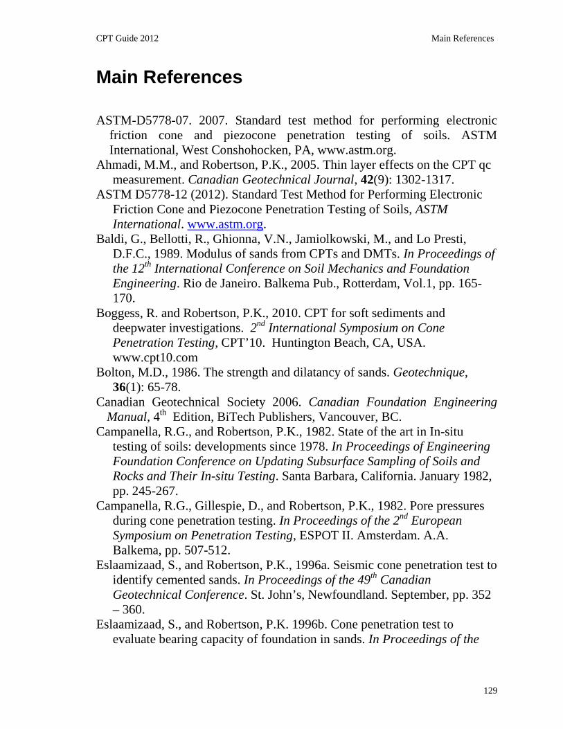
CPT Guide 2012 Main References
129
Main References
ASTM-D5778-07. 2007. Standard test method for performing electronicfriction cone and piezocone penetration testing of soils. ASTMInternational, West Conshohocken, PA, www.astm.org.
Ahmadi, M.M., and Robertson, P.K., 2005. Thin layer effects on the CPT qcmeasurement. Canadian Geotechnical Journal, 42(9): 1302-1317.
ASTM D5778-12 (2012). Standard Test Method for Performing ElectronicFriction Cone and Piezocone Penetration Testing of Soils, ASTMInternational. www.astm.org.
Baldi, G., Bellotti, R., Ghionna, V.N., Jamiolkowski, M., and Lo Presti,D.F.C., 1989. Modulus of sands from CPTs and DMTs. In Proceedings ofthe 12th International Conference on Soil Mechanics and FoundationEngineering. Rio de Janeiro. Balkema Pub., Rotterdam, Vol.1, pp. 165-170.
Boggess, R. and Robertson, P.K., 2010. CPT for soft sediments anddeepwater investigations. 2nd International Symposium on ConePenetration Testing, CPT’10. Huntington Beach, CA, USA.www.cpt10.com
Bolton, M.D., 1986. The strength and dilatancy of sands. Geotechnique,36(1): 65-78.
Canadian Geotechnical Society 2006. Canadian Foundation EngineeringManual, 4th Edition, BiTech Publishers, Vancouver, BC.
Campanella, R.G., and Robertson, P.K., 1982. State of the art in In-situtesting of soils: developments since 1978. In Proceedings of EngineeringFoundation Conference on Updating Subsurface Sampling of Soils andRocks and Their In-situ Testing. Santa Barbara, California. January 1982,pp. 245-267.
Campanella, R.G., Gillespie, D., and Robertson, P.K., 1982. Pore pressuresduring cone penetration testing. In Proceedings of the 2nd EuropeanSymposium on Penetration Testing, ESPOT II. Amsterdam. A.A.Balkema, pp. 507-512.
Eslaamizaad, S., and Robertson, P.K., 1996a. Seismic cone penetration test toidentify cemented sands. In Proceedings of the 49th CanadianGeotechnical Conference. St. John’s, Newfoundland. September, pp. 352– 360.
Eslaamizaad, S., and Robertson, P.K. 1996b. Cone penetration test toevaluate bearing capacity of foundation in sands. In Proceedings of the

CPT Guide - 2012 Main References
130
49th Canadian Geotechnical Conference. St. John’s, Newfoundland.September, pp. 429-438.
Eslaamizaad, S. and Robertson, P.K., 1997. Evaluation of settlement offootings on sand from seismic in-sity tests. In Proceedings of the 50th
Canadian Geotechnical Conference, Ottawa, Ontario, October 1997,Vol.2, pp. 755-764.
Fahey, M. and Carter, J.P., 1993. A finite element study of the pressuremeterin sand using a nonlinear elastic plastic model. Canadian GeotechnicalJournal, 30(2): 348-362.
Hight, D., and Leroueil, S., 2003. Characterization of soils for engineeringpurposes. Characterization and Engineering Properties of Natural Soils,Vol.1, Swets and Zeitlinger, Lisse, pp. 255-360.
Idriss, I.M. and Boulanger, R.W., 2004. Semi-empirical procedures forevaluating liquefaction potential during earthquakes. Proceedings 11th
International Conference on Soil Dynamics and Earthquake Engineering.Berkeley, 32-56.
IRTP, 1999. International Reference Test Procedure for Cone PenetrationTest (CPT). Report of the ISSMFE Technical Committee on PenetrationTesting of Soils, TC 16, Swedish Geotechnical Institute, Linkoping,Information, 7, 6-16.
Janbu, N., 1963, Soil Compressibility as determined by oedometer andtriaxial tests. Proceedings of the European Conference on SoilMechanicxs and Foundation Engineering, Wiesbaden, pp 19-25.
Jamiolkowski, M., Ladd, C.C., Germaine, J.T., and Lancellotta, R., 1985.New developments in field and laboratory testing of soils. In Proceedingsof the 11th International Conference on Soil Mechanics and FoundationEngineering. San Francisco, California, August 1985, Vol.1 pp. 57-153.
Jefferies, M.G., and Davies, M.O, 1991. Soil Classification by the conepenetration test: discussion. Canadian Geotechnical Journal, 28(1): 173-176.
Jefferies, M.G., and Davies, M.P., 1993. Use of CPTU to estimate equivalentSPT N60. Geotechnical Testing Journal, ASTM, 16(4): 458-468.
Jefferies, M.G. and Been, K., 2006. Soil Liquefaction – A critical stateapproach. Taylor & Francis, ISBN 0-419-16170-8 478 pages.
Kayen, R., Moss, R.E.S., Thompson, E.M., Seed, R.B., Cetin, K.O., DerKiureghian, A., Tanaka, Y., and Tokimatsu, K., 2013. Shear-wavevelocity-based probabilistic and deterministic assessment of seismic soilliquefaction potential, J. of Geotech. and Geoenvironmental Engineering,ASCE, 2013.139: 407-419.

CPT Guide 2012 Main References
131
Karlsrud, K., Lunne, T., Kort, D.A. & Strandvik, S. 2005. CPTU correlationsfor Clays. Proc. 16th ICSMGE, Osaka, September 2005
Kulhawy, F.H., and Mayne, P.H., 1990. Manual on estimating soil propertiesfor foundation design, Report EL-6800 Electric Power Research Institute,EPRI, August 1990.
Ladd, C.C., and Foott, R. (1974). "New design procedure for stability of softclays." J. of the Geotech. Eng. Div., 100(GT7), 763-786.
Ladd, C.C. & DeGroot, D.J. 2003. Recommended practice for soft groundsite characterization. Soil and Rock America, Vol. 1 (Proc.12thPanAmerican Conf., MIT), Verlag Glückauf, Essen: 3-57.
Lunne, T., Eidsmoen, T., Gillespie, D., and Howland, J.D., 1986. Laboratoryand field evaluation on cone penetrometers. Proceedings of ASCESpecialty Conference In Situ’86: Use of In Situ Tests in GeotechnicalEngineering. Blacksburg, ASCE, GSP 6 714-729
Lunne, T., Robertson, P.K., and Powell, J.J.M., 1997. Cone penetrationtesting in geotechnical practice. Blackie Academic, EF Spon/RoutledgePubl., New York, 1997, 312 pp.
Lunne, T., and Andersen, K.H., 2007. Soft clay shear strength parameters fordeepwater geotechnical design. Proceedings 6th InternationalConference, Society for Underwater Technology, Offshore SiteInvestigation and Geomechanics, London, 151-176.
Mayne, P.W., 2000. Enhanced Geotechnical Site Characterization bySeismic Piezocone Penetration Test. Invited lecture, Fourth InternationalGeotechnical Conference, Cairo University. pp 95-120.
Mayne, P.W., 2005. Integrated Ground Behavior: In-Situ and Lab Tests,Deformation Characteristics of Geomaterials, Vol. 2 (Proc. Lyon), Taylor& Francis, London, pp. 155-177.
Mayne, P.W., 2007. NCHRP Synthesis ‘Cone Penetration Testing State-of-Practice’. Transportation Research Board Report Project 20-05. 118pages. www.trb.org
Mayne, P.W., 2008. Piezocone profiling of clays for maritime siteinvestigations. 11th Baltic Sea Geotechnical Conference. Gdansk,Poland., 151- 178.
Mayne, P.W., Coop, M.R., Springman, S.M., Huang, A.B, and Zornberg,J.G., 2009. Geomaterail behaviour and testing. State of the Art (SOA)paper, 17th ICSMGE Alexandria.
Mitchell, J.K., Guzikowski, F. and Villet, W.C.B., 1978. The Measurementof Soil Properties In-Situ, Report prepared for US Department of EnergyContract W-7405-ENG-48, Lawrence Berkeley Laboratory, University ofCalifornia, Berkeley, CA, 94720.

CPT Guide - 2012 Main References
132
Molle, J., 2005. The accuracy of the interpretation of CPT-based soilclassification methods in soft soils. MSc Thesis, Section for EngineeringGeology, Department of Applied Earth Sciences, Delf University ofTechnology, Report No. 242, Report AES/IG/05-25, December
Parez, L. and Faureil, R., 1988. Le piézocône. Améliorations apportées à lareconnaissance de sols. Revue Française de Géotech, Vol. 44, 13-27.
Robertson, P.K., 1990. Soil classification using the cone penetration test.Canadian Geotechnical Journal, 27(1): 151-158.
Robertson, P.K., 1998. Risk-based site investigation. Geotechnical News: 45-47, September 1998.
Robertson, P.K., 2009a. Interpretation of cone penetration tests – a unifiedapproach. Canadian Geotechnical Journal, 46:1337-1355.
Robertson, P.K., 2010a. Soil behaviour type from the CPT: an update. 2nd
International Symposium on Cone Penetration Testing, CPT’10,Huntington Beach, CA, USA. www.cpt10.com
Robertson, P.K., 2010b. Estimating in-situ state parameter and friction anglein sandy soils from the CPT. 2nd International Symposium on ConePenetration Testing, CPT’10, Huntington Beach, CA, USA.www.cpt10.com
Robertson, P.K., 2010c. Evaluation of Flow Liquefaction and Liquefiedstrength Using the Cone Penetration Test. Journal of Geotechnical andGeoenvironmental Engineering, ASCE, 136(6): 842-853
Robertson. P.K., Campanella, R.G., Gillespie, D., and Greig, J., 1986. Useof Piezometer Cone data. In-Situ’86 Use of Ins-itu testing inGeotechnical Engineering, GSP 6 , ASCE, Reston, VA, SpecialtyPublication, SM 92, pp 1263-1280.
Robertson, P.K., Sully, J.P., Woeller, D.J., Lunne, T., Powell, J.J.M. andGillespie, D., 1992. Estimating coefficient of consolidation frompiezocone tests. Canadian Geotechnical Journal, Ottawa, 29(4): 539-550.
Robertson, P.K., and Campanella, R.G., 1983a. Interpretation of conepenetration tests – Part I (sand). Canadian Geotechnical Journal, 20(4):718-733.
Robertson, P.K., and Campanella, R.G. 1983b. Interpretation of conepenetration tests – Part II (clay). Canadian Geotechnical Journal, 20(4):734-745.
Robertson, P.K. and Wride, C.E., 1998. Evaluating cyclic liquefactionpotential using the cone penetration test. Canadian Geotechnical Journal,Ottawa, 35(3): 442-459.

CPT Guide 2012 Main References
133
Robertson, P.K., Campanella, R.G., Gillespie, D., and Rice, A., 1986.Seismic CPT to measure in-situ shear wave velocity. Journal ofGeotechnical Engineering Division, ASCE, 112(8): 791-803.
Sanglerat, G., 1972. The Penetrometer and Soil Exploration. Elsevier Pub.,Amsterdam, 488pp.
Schnaid, F., 2005. Geocharacterization and Engineering properties of naturalsoils by in-situ tests. In Proceedings of the 16th International Conferenceon Soil Mechanics and Geotechnical Engineering, Vol.1, Osaka,September, 2005, Millpress, Rotterdam, pp. 3-45.
Schneider, J.A., Randolph, M.F., Mayne, P.W. & Ramsey, N.R. 2008.Analysis of factors influencing soil classification using normalizedpiezocone tip resistance and pore pressure parameters. JournalGeotechnical and Geoenvironmental Engrg. 134 (11): 1569-1586.
Schmertmann, J.H. 1978. Guidelines for cone penetration tests performanceand design. Federal Highways Administration, Washington, D.C., ReportFHWA-TS-78-209.
Teh, C.I., and Houlsby, G.T. 1991. An analytical study of the conepenetration test in clay. Geotechnique, 41 (1): 17-34.
Wride, C.E., Robertson, P.K., Biggar, K.W., Campanella, R.G., Hofmann,B.A., Hughes, J.M.O., Küpper, A., and Woeller, D.J. In-Situ testingprogram at the CANLEX test sites. Canadian Geotechnical Journal,2000, Vol. 37, No. 3, June, pp. 505-529
Wroth, C.P., 1984. The interpretation of in-situ soil tests. Rankine Lecture,Geotechnique(4).
Youd, T.L., Idriss, I.M., Andrus, R.D., Arango, I., Castro, G., Christian, J.T.,Dobry, R., Finn, W.D.L., Harder, L.F., Hynes, M.E., Ishihara, K.,Koester, J., Liao, S., Marcuson III, W.F., Martin, G.R., Mitchell, J.K.,Moriwaki, Y., Power, M.S., Robertson, P.K., Seed, R., and Stokoe, K.H.,Liquefaction Resistance of Soils: Summary Report from the 1996 NCEERand 1998 NCEER/NSF Workshop on Evaluation of LiquefactionResistance of Soils, ASCE, Journal of Geotechnical & GeoenvironmentalEngineering, Vol. 127, October, pp 817-833
Zhang, Z., and Tumay, M.T., 1999. Statistical to fuzzy approach toward CPTsoil classification. Journal of Geotechnical and GeoenvironmentalEngineering, 125(3): 179-186.
Zhang, G., Robertson, P.K. and Brachman, R.W.I., 2002, EstimatingLiquefaction induced Ground Settlements From CPT for Level Ground,Canadian Geotechnical Journal, 39(5): 1168-1180