Keywords: cone penetration test, CPT, cone resistance, sands, in-situ tests

COMPUTATION OF CAVITY EXPANSION PRESSURE AND PENETRATION

RESISTANCE IN SANDS

By R. Salgado,1 M. ASCE and M. Prezzi,2 A.M., ASCE

ABSTRACT

A cavity expansion-based theory for calculation of cone penetration resistance qc in sand is

presented. The theory includes a completely new analysis to obtain cone resistance from

cavity limit pressure. In order to more clearly link the proposed theory with the classical

cavity expansion theories, which were based on linear elastic, perfectly plastic soil response,

linear equivalent values of elasticity modulus, Poisson's ratio and friction and dilatancy

angles are given in charts as a function of relative density, stress state, and critical-state

friction angle. These linear-equivalent values may be used in the classical theories to obtain

very good estimates of cavity pressure. A much simpler way to estimate qc -- based on direct

reading from charts in terms of relative density, stress state and critical state friction angle –

is also proposed. Finally, a single equation obtained by regression of qc on relative density

and stress state for a range of values of critical state friction angle is also proposed.

Examples illustrate the different ways of calculating cone resistance and interpreting cone

penetration test results.

INTRODUCTION

The cone penetration test (CPT) is now widely used for geotechnical site

characterization and in-situ determination of soil properties. Among its advantages are

simplicity, speed, and continuous profiling. Originally, the penetrometer was used to 1 Prof., School of Civil Engrg., 550 Stadium Mall Dr., Purdue Univ., West Lafayette, IN

47907-2051, phone: (765) 494-5030, fax: (765) 496-1364, rodrigo@ecn.purdue.edu 2 Assistant Prof., School of Civil Engrg., 550 Stadium Mall Dr., Purdue Univ., West

Lafayette, IN 47907-2051, phone: (765) 494-5034, fax: (765) 496-1364, mprezzi@ecn.purdue.edu

2

measure only tip resistance, defined as the vertical force acting on the tip of the penetrometer

divided by the base area of the tip (10 cm2 for the standard 35.7-mm diameter penetrometer).

Over the years, sensors have been incorporated into the cone to measure the friction along a

lateral sleeve, the arrival of a seismic shear wave (which allows determining shear wave

velocities), pore pressure, and other quantities (Mitchell 1988). This versatility has further

enhanced the use of the CPT. In addition, an important advantage of the CPT is that the

penetration process is amenable to theoretical modeling.

A general penetration resistance theory allowing calculation of penetration resistance

in geologically recent, uncemented, clean sands was developed by Salgado et al. (1997a) and

codified into the program CONPOINT. Predictions by this theory were extensively and

successfully tested against actual measurements of penetration resistance made in calibration

chambers (Salgado et al. 1997a,b; 1998) and in the field (Lee et al. 1999; Bonita 2000).

The cone penetration resistance analysis has evolved in various ways since it was first

presented in Salgado et al. (1997a). Most notably, limit pressure is calculated in a much

more effective way, and a new formulation for calculating cone resistance from cavity limit

pressure (which considers the true interface friction angle between the cone and soil) has

been developed and implemented. These developments are presented in this paper.

Moreover, the cavity expansion analysis on which the cone resistance analysis is largely

based, is linked to the classical cavity expansion analyses, all based on linear elasticity and

perfect plasticity, by the presentation of values of friction and dilatancy angles, elasticity

modulus and Poisson's ratio that, once plugged in those analyses, would produce

substantially the same values of cavity expansion limit pressure as the present theory.

In practice, engineers often use simplified equations and charts. Two additional

methods of penetration resistance estimation, one relying on charts of cone resistance qc

expressed directly in terms of density and stress, the other on simple expressions of qc in

terms of relative density and stress state, are given. Examples illustrate the application of

these different methods to cone resistance interpretation.

3

CAVITY EXPANSION ANALYSIS

Analytical Solutions

Originally, cavity expansion analysis aimed to solve problems of metal indentation

(Bishop et al. 1945, Hill 1950), which became more important as the industrial revolution

intensified in the last part of the 19th century and first half of the 20th century. So, in its

origins, cavity expansion analysis was very much linked to a penetration process, but a

penetration process in a much simpler material (one typically assumed to follow the Tresca

or Mises yield criterion and to have zero dilatancy). It is interesting that the results these

pioneers obtained support facts we now accept for penetration processes in soil, such as the

value of the ratio of qc to undrained shear strength in clays and the need to push a

penetrometer down several diameters before a steady state pressure is achieved.

After metal indentation, weapons research stimulated by the cold war, motivated

further research on cavity expansion, notably the work of Chadwick (1959, 1962), who first

introduced friction into the analysis, adopting the Mohr-Coulomb criterion with an associated

flow rule. The interests then were related to explosions within the ground and how the stress

waves generated by these explosions would propagate. Geomechanics with more of a

geotechnical engineering flavor followed, notably with works by Ladanyi (1963), who was

interested in cavity expansion in clays, and Palmer (1972), who studied applications of cavity

expansion analyses to the pressuremeter test. There was some further work by Vesic (1972)

and Baligh (1976), who attempted to capture the important feature of soil stress-strain non-

linearity, but in a way that was empirically based. The next generation of analyses appeared

in the 1980's, 1990's and 2000's (notably, Carter et al. 1986, Yu and Houlsby 1989, Collins et

4

al. 1992, Salgado et a. 1997 and Salgado and Randolph 2001). In the discussion that follows,

we focus on the closed-form analyitical solutions of Carter et al. (1986) and Yu and Houlsby

(1989) for linear elastic, perfectly plastic soil.

In this paper, our focus is on penetration processes, which are associated with cavity

creation in the soil. If a cavity is expanded from a finite initial radius, an increasing pressure

is always required for continued expansion. In contrast, in a cavity creation process, the

cavity is expanded from zero initial radius and therefore immediately reaches a steady-state

condition. In the steady-state condition, ongoing expansion happens at constant cavity

pressure; this pressure is referred to as the limit pressure pL.

Relationship to Penetration Resistance

Penetration resistance, whether cone resistance qc or limit unit base resistance qbL,

can be related to the relevant intrinsic soil variables and soil state variables. The intrinsic

variables depend only on the nature of the sand particles (the mineralogy, size, shape, and

surface characteristics of the soil particles). In uncemented, cohesionless soils, the relevant

state variables are relative density DR and effective stress state3 (σv and σh).

When a penetrometer is pushed vertically in the soil, it creates and expands a

cylindrical cavity. Thus, there is a relationship between penetration resistance and the

pressure required to expand a cylindrical cavity in the soil from zero initial radius. The

cylindrical cavity expansion pressure is a function of the initial lateral effective stress σh =

Koσv in the soil. Sands with a given vertical effective stress can have different lateral

effective stresses, and, therefore, different qc values, if the overconsolidation ratios (and

5

therefore Ko) are different. Experimental evidence (Jamiolkowski et al. 1985, Baldi et al.

1986, Houlsby and Hitchman 1988, Houlsby and Wroth 1989, Mayne and Kulhawy 1991)

indicates that qc correlates quite well with the stress state as expressed by the lateral effective

stress σh, providing additional support for relating qc (and qbL) to the cylindrical cavity limit

pressure.

Numerical Cavity Expansion Formulation

Plastic Zone

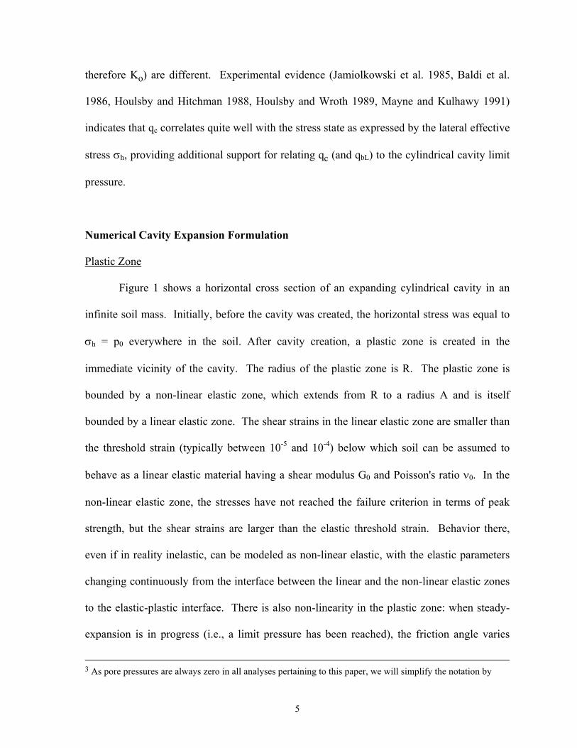
Figure 1 shows a horizontal cross section of an expanding cylindrical cavity in an

infinite soil mass. Initially, before the cavity was created, the horizontal stress was equal to

σh = p0 everywhere in the soil. After cavity creation, a plastic zone is created in the

immediate vicinity of the cavity. The radius of the plastic zone is R. The plastic zone is

bounded by a non-linear elastic zone, which extends from R to a radius A and is itself

bounded by a linear elastic zone. The shear strains in the linear elastic zone are smaller than

the threshold strain (typically between 10-5 and 10-4) below which soil can be assumed to

behave as a linear elastic material having a shear modulus G0 and Poisson's ratio ν0. In the

non-linear elastic zone, the stresses have not reached the failure criterion in terms of peak

strength, but the shear strains are larger than the elastic threshold strain. Behavior there,

even if in reality inelastic, can be modeled as non-linear elastic, with the elastic parameters

changing continuously from the interface between the linear and the non-linear elastic zones

to the elastic-plastic interface. There is also non-linearity in the plastic zone: when steady-

expansion is in progress (i.e., a limit pressure has been reached), the friction angle varies

3 As pore pressures are always zero in all analyses pertaining to this paper, we will simplify the notation by

6

from a value equal to the critical state friction angle φc at the cavity wall to a value equal to

the peak friction angle φp at the elastic-plastic interface.

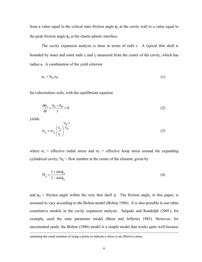
The cavity expansion analysis is done in terms of radii r. A typical thin shell is

bounded by inner and outer radii ri and rj measured from the center of the cavity, which has

radius a. A combination of the yield criterion

σr = Nij σθ (1)

for cohesionless soils, with the equilibrium equation

r rd 0

dr rθσ σ − σ

+ = (2)

yields ij

iji j

N 1Nj

r ri

rr

−

σ = σ

(3)

where σr = effective radial stress and σθ = effective hoop stress around the expanding

cylindrical cavity; Nij = flow number at the center of the element, given by

ij

ijij sin1

sin1N

φ−φ+

= (4)

and φij = friction angle within the very thin shell ij. The friction angle, in this paper, is

assumed to vary according to the Bolton model (Bolton 1986). It is also possible to use other

constitutive models in the cavity expansion analysis. Salgado and Randolph (2001), for

example, used the state parameter model (Been and Jefferies 1985). However, for

uncemented sands, the Bolton (1986) model is a simple model that works quite well because ommiting the usual notation of using a prime to indicate a stress is an effective stress.

7

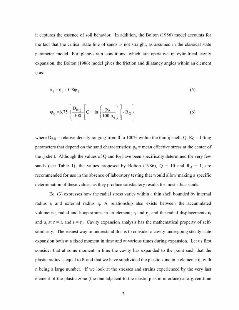
it captures the essence of soil behavior. In addition, the Bolton (1986) model accounts for

the fact that the critical state line of sands is not straight, as assumed in the classical state

parameter model. For plane-strain conditions, which are operative in cylindrical cavity

expansion, the Bolton (1986) model gives the friction and dilatancy angles within an element

ij as:

ijcij 8.0 = ψ+φφ (5)

R,ij Aij Q

ij

D p =6.75 Q + ln - R100 100 p

ψ (6)

where DR,ij = relative density ranging from 0 to 100% within the thin ij shell; Q, RQ = fitting

parameters that depend on the sand characteristics; pij = mean effective stress at the center of

the ij shell. Although the values of Q and RQ have been specifically determined for very few

sands (see Table 1), the values proposed by Bolton (1986), Q = 10 and RQ = 1, are

recommended for use in the absence of laboratory testing that would allow making a specific

determination of these values, as they produce satisfactory results for most silica sands.

Eq. (3) expresses how the radial stress varies within a thin shell bounded by internal

radius ri and external radius rj. A relationship also exists between the accumulated

volumetric, radial and hoop strains in an element; ri and rj; and the radial displacements ui

and uj at r = ri and r = rj. Cavity expansion analysis has the mathematical property of self-

similarity. The easiest way to understand this is to consider a cavity undergoing steady state

expansion both at a fixed moment in time and at various times during expansion. Let us first

consider that at some moment in time the cavity has expanded to the point such that the

plastic radius is equal to R and that we have subdivided the plastic zone in n elements ij, with

n being a large number. If we look at the stresses and strains experienced by the very last

element of the plastic zone (the one adjacent to the elastic-plastic interface) at a given time

8

and by the element next to it (in the direction of the cavity) at end of the previous time

increment, when it was the outermost element of the plastic zone, we see that they are

identical. This is true of any other pair of elements in the plastic zone: the stresses and

strains in an element at a given time are the same as the ones experienced by the element

interior to it at end of the previous time increment. The outer element experiences conditions

identical to those experienced by the inner element one time increment earlier in the cavity

expansion process. This fact can be used to calculate the strain increments for the same

element when the plastic radius R increases by some small amount during cavity expansion.

These strain increments are tied together by the dilatancy angle, following the flow rule of

Rowe (1962). Salgado and Randolph (2001) present the mathematics of how this is done in

cavity expansion analysis. Starting from the plastic radius, where stresses, strains and the

radial displacement are known, calculations proceed inward, towards the cavity, element by

element. At the elastic-plastic interface, the radial stress σR and the mean effective stress pR

are given by (Salgado et al. 1997a, Salgado and Randolph 2001):

p

R 0p

2Np

N 1σ =

+ (7)

R R Rp

1 1p [1 ] 13 N

= + µ + σ

(8)

with

)sinsin1(21

ppR ψφ+=µ (9)

p 0RT

p

N 1 puR N k 2G

−ε = − =

+ (10)

εr(r=R) = εR = k εT (11)

9

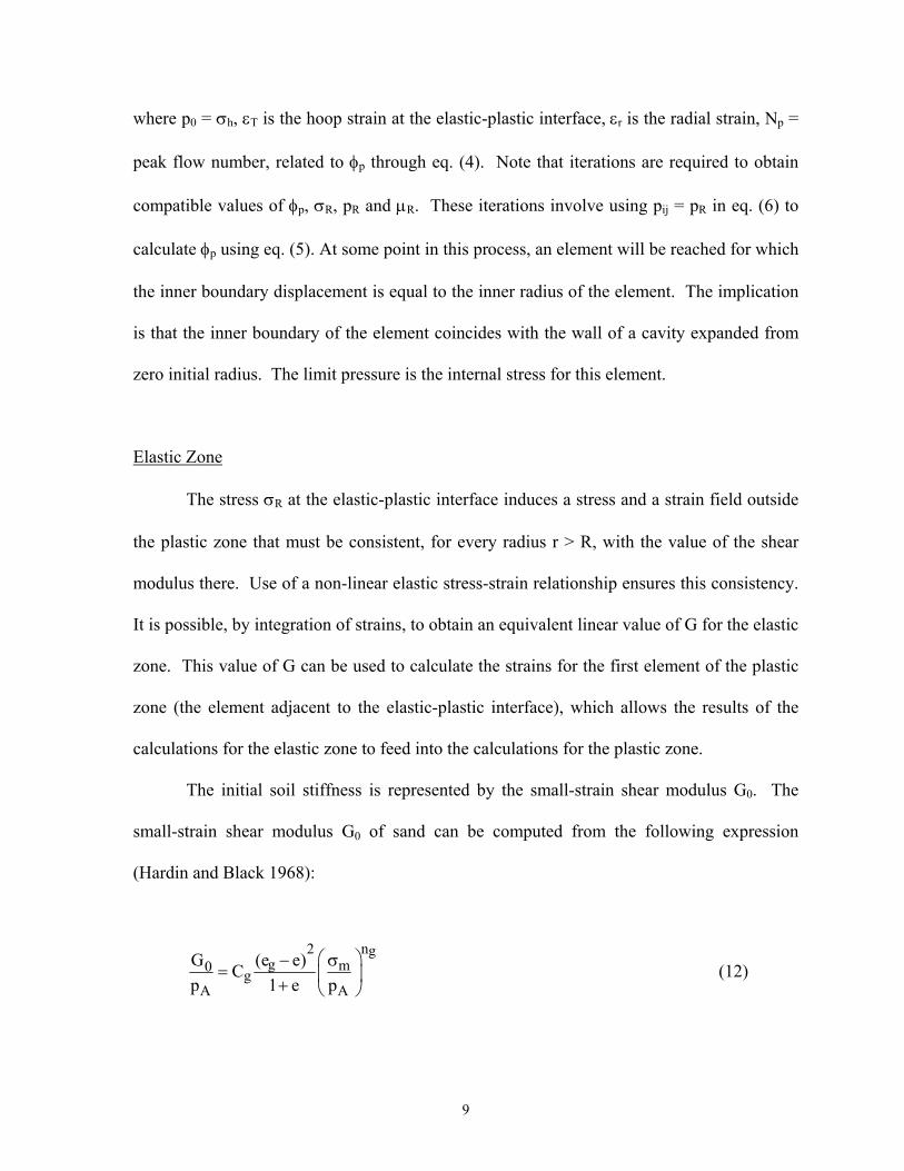
where p0 = σh, εT is the hoop strain at the elastic-plastic interface, εr is the radial strain, Np =

peak flow number, related to φp through eq. (4). Note that iterations are required to obtain

compatible values of φp, σR, pR and µR. These iterations involve using pij = pR in eq. (6) to

calculate φp using eq. (5). At some point in this process, an element will be reached for which

the inner boundary displacement is equal to the inner radius of the element. The implication

is that the inner boundary of the element coincides with the wall of a cavity expanded from

zero initial radius. The limit pressure is the internal stress for this element.

Elastic Zone

The stress σR at the elastic-plastic interface induces a stress and a strain field outside

the plastic zone that must be consistent, for every radius r > R, with the value of the shear

modulus there. Use of a non-linear elastic stress-strain relationship ensures this consistency.

It is possible, by integration of strains, to obtain an equivalent linear value of G for the elastic

zone. This value of G can be used to calculate the strains for the first element of the plastic

zone (the element adjacent to the elastic-plastic interface), which allows the results of the

calculations for the elastic zone to feed into the calculations for the plastic zone.

The initial soil stiffness is represented by the small-strain shear modulus G0. The

small-strain shear modulus G0 of sand can be computed from the following expression

(Hardin and Black 1968):

n2 g

g m0 gA A

G (e e)Cp 1 e p

− σ= +

(12)

10

where e = initial void ratio; σm = p = initial mean effective stress; Cg, eg, ng = intrinsic

variables of the soil.

Relationship to Analytical Cavity Expansion Solutions

Limit Cavity Pressure

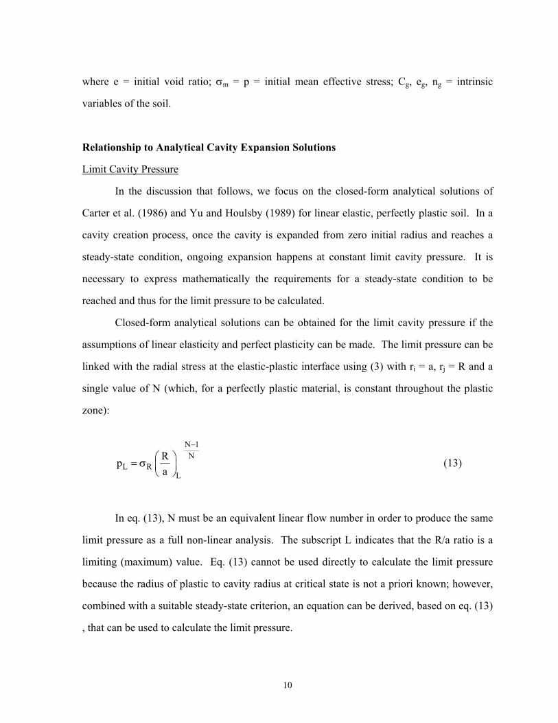
In the discussion that follows, we focus on the closed-form analytical solutions of

Carter et al. (1986) and Yu and Houlsby (1989) for linear elastic, perfectly plastic soil. In a

cavity creation process, once the cavity is expanded from zero initial radius and reaches a

steady-state condition, ongoing expansion happens at constant limit cavity pressure. It is

necessary to express mathematically the requirements for a steady-state condition to be

reached and thus for the limit pressure to be calculated.

Closed-form analytical solutions can be obtained for the limit cavity pressure if the

assumptions of linear elasticity and perfect plasticity can be made. The limit pressure can be

linked with the radial stress at the elastic-plastic interface using (3) with ri = a, rj = R and a

single value of N (which, for a perfectly plastic material, is constant throughout the plastic

zone):

N 1N

L RL

Rpa

−

= σ

(13)

In eq. (13), N must be an equivalent linear flow number in order to produce the same

limit pressure as a full non-linear analysis. The subscript L indicates that the R/a ratio is a

limiting (maximum) value. Eq. (13) cannot be used directly to calculate the limit pressure

because the radius of plastic to cavity radius at critical state is not a priori known; however,

combined with a suitable steady-state criterion, an equation can be derived, based on eq. (13)

, that can be used to calculate the limit pressure.

11

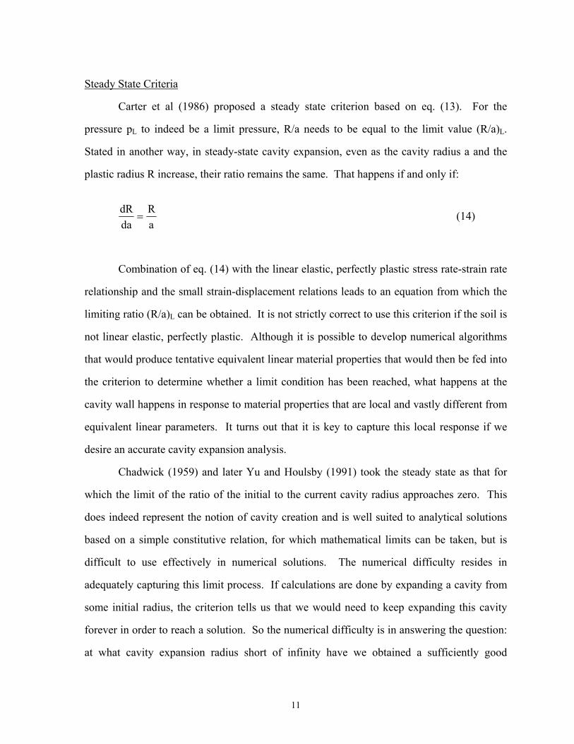
Steady State Criteria

Carter et al (1986) proposed a steady state criterion based on eq. (13). For the

pressure pL to indeed be a limit pressure, R/a needs to be equal to the limit value (R/a)L.

Stated in another way, in steady-state cavity expansion, even as the cavity radius a and the

plastic radius R increase, their ratio remains the same. That happens if and only if:

dRda

Ra

= (14)

Combination of eq. (14) with the linear elastic, perfectly plastic stress rate-strain rate

relationship and the small strain-displacement relations leads to an equation from which the

limiting ratio (R/a)L can be obtained. It is not strictly correct to use this criterion if the soil is

not linear elastic, perfectly plastic. Although it is possible to develop numerical algorithms

that would produce tentative equivalent linear material properties that would then be fed into

the criterion to determine whether a limit condition has been reached, what happens at the

cavity wall happens in response to material properties that are local and vastly different from

equivalent linear parameters. It turns out that it is key to capture this local response if we

desire an accurate cavity expansion analysis.

Chadwick (1959) and later Yu and Houlsby (1991) took the steady state as that for

which the limit of the ratio of the initial to the current cavity radius approaches zero. This

does indeed represent the notion of cavity creation and is well suited to analytical solutions

based on a simple constitutive relation, for which mathematical limits can be taken, but is

difficult to use effectively in numerical solutions. The numerical difficulty resides in

adequately capturing this limit process. If calculations are done by expanding a cavity from

some initial radius, the criterion tells us that we would need to keep expanding this cavity

forever in order to reach a solution. So the numerical difficulty is in answering the question:

at what cavity expansion radius short of infinity have we obtained a sufficiently good

12

approximation? While approximations can be found, it would be difficult to control the

accuracy of a numerical solution based on this criterion.

In this paper, the steady state criterion used is that the calculated displacement at the

inner boundary of the cylindrical element must equal its inner radius. This expresses the

physical notion of cavity creation rigorously and has the advantage of being easily

implemented in a numerical formulation.

Equivalent Linear Values of Plastic and Elastic Parameters

Engineers wishing to use the analytical cavity expansion solutions need guidance on

which values of shear modulus and friction and dilatancy angles to use. The present analysis

can produce these values. It is of particular interest to investigate how the equivalent linear

values of φ, ψ, E and ν vary with initial soil state, i.e., initial relative density and stress state.

For this purpose, calculations are done for the following values of the intrinsic values Cg, eg,

ng, emin, emax, Q and RQ:

Cg = 650 eg = 2.2 ng = 0.45

emin = 0.60 emax = 0.95

Q = 10 RQ = 1

These values are representative of typical silica sands. The relative density values

considered are DR = 10, 20, 30, 40, 50, 60, 70, 80, 90 and 100%. The coefficient of active

lateral stress is in the 0.4 to 0.5 in most cases in practice, with dense sands tending to have

lower, and loose sands, higher values. For simplicity, a single value of 0.45 is taken for all

values of relative density. The maximum vertical effective stress considered is that for a

depth z = 50m and water table deeper than 50m. Taking the unit weight as roughly 20kN/m3,

this would correspond to 1MPa vertical effective stress. Values are varied from 50kPa to

1MPa in 50kPa increments.

13

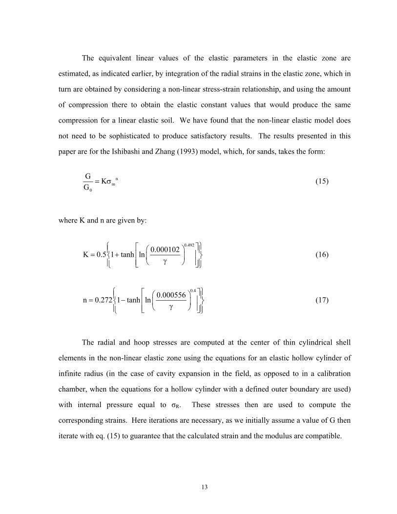
The equivalent linear values of the elastic parameters in the elastic zone are

estimated, as indicated earlier, by integration of the radial strains in the elastic zone, which in

turn are obtained by considering a non-linear stress-strain relationship, and using the amount

of compression there to obtain the elastic constant values that would produce the same

compression for a linear elastic soil. We have found that the non-linear elastic model does

not need to be sophisticated to produce satisfactory results. The results presented in this

paper are for the Ishibashi and Zhang (1993) model, which, for sands, takes the form:

n

m0

G KG

= σ (15)

where K and n are given by:

0.492

0.000102K 0.5 1 tanh ln = + γ

(16)

0.4

0.000556n 0.272 1 tanh ln = − γ

(17)

The radial and hoop stresses are computed at the center of thin cylindrical shell

elements in the non-linear elastic zone using the equations for an elastic hollow cylinder of

infinite radius (in the case of cavity expansion in the field, as opposed to in a calibration

chamber, when the equations for a hollow cylinder with a defined outer boundary are used)

with internal pressure equal to σR. These stresses then are used to compute the

corresponding strains. Here iterations are necessary, as we initially assume a value of G then

iterate with eq. (15) to guarantee that the calculated strain and the modulus are compatible.

14

The equivalent linear shear modulus normalized with respect to the small-strain shear

modulus, G/G0, is plotted in Figure 2 for φc = 29° and φc = 36°. It can be seen that G/G0 does

not vary much with relative density or φc, but does vary significantly with lateral effective

stress. For σh = 22.5kPa, G/G0 lies in the 0.52-0.6 range for φc = 29° and in the 0.5 to 0.58

range for φc = 36°. For σh = 450kPa, G/G0 lies in the 0.86-0.9 range for φc = 29° and in the

0.8 to 0.88 range for φc = 36°.

The linear-equivalent flow number N in the plastic zone at steady state can be

determined from the rigorous analysis by considering directly eq. (13). For a given plastic

radius R, the analysis produces values of σR, pL and a at steady state. It follows that N can be

calculated as:

L

L

RL

Rlna

NpRln ln

a

=

− σ

(18)

The linear equivalent friction angle φ is then obtained from N through the general

equation relating flow number to friction angle:

N 1sinN 1

−φ =

+ (19)

Once φ is known, the linear-equivalent dilatancy angle can be obtained from the

values of φ and φc using eq. (6). The φ calculated using eq. (19) is plotted in Figure 3. The

figure shows a plot of φ - φc vs. initial lateral stress for three values of critical-state friction

angle φc: 29, 33 and 36°. This covers the full range of φc values for silica sands. It can be

seen from the figure that the plots are in essence independent of φc for DR = 0–60% but start

15

separating for larger relative densities. Even so, for DR = 100%, the difference between φ -

φc values for φc = 29° and φc = 36° is only of the order of one degree.

It is interesting to explore how the ratio (R/a)L of the plastic radius to the cavity

radius at the limit condition (when the limit pressure has been reached) varies with initial soil

state. This is a quantity of interest not only in that it is an integral part of the calculations of

limit pressure but also in that the question of how far the effects of cavity creation extend is

often asked in practical problems. For example, if experiments are being conducted on

penetrometers, the question of how far a boundary can be placed without excessively

distorting the mechanism the experiments aim to study is an important one, and the extent of

the plastic zone can guide us on that account.

Figure 4 shows (R/a)L vs. lateral effective stress for φc = 29° and φc = 36° and DR =

10-100%. Note first that the values of (R/a)L are practically independent of φc. Note also

that the plastic radius to cavity radius ratio is greater than 100 for dense sands and as high as

70 for medium dense sands at low confining stresses (0-50kPa), which correspond to depths

often of interest in geotechnical engineering problems. This means that the use of calibration

chambers or centrifuges to study cone penetration must be guided by rigorous theory,

because of the existence of boundary effects (excessive proximity of chamber boundaries to

the cone, interfering with the formation of the plastic zone around it), which can be

substantial, particularly for shallow penetration. These plots of (R/a)L can be used to obtain

suitable values of (R/a)L for use in eq. (13). Since the radial stress at the elastic-plastic

interface follows from eq. (7), limit cavity pressures can then be calculated using eq. (13). A

more direct way to obtain limit pressure is to use the charts in Figure 5, in which limit

pressure vs. initial lateral effective stress is plotted for DR = 10-100% and φc ranging from 29

to 36°. There is a gradual shift to the right in the pL versus stress curves as φc increases from

29 to 36°. The maximum limit pressure, calculated for DR = 100% and 1MPa vertical stress

(450 kPa lateral stress), is approximately 15MPa.

16

PENETRATION RESISTANCE ANALYSIS

Basic Analysis for Cone Penetrometers

The penetration resistance of a penetrometer with flat or conical tip may be calculated

from the limit pressure pL determined in the previous section. Although a rigorous analysis

that incorporates all the main features of sand mechanical response would be very difficult,

an analysis with sufficient accuracy can be obtained if a few simplifying assumptions are

made.

Figure 6 shows a plane-strain, kinematically admissible slip mechanism that can be

used to develop a suitable analysis. If we can assume a similar mechanism exists for a

penetrometer with a conical tip, the conical surface, during penetration, is in effect a slip

surface with interface friction angle δc. The semi-apex angle of the cone is θc. From the

point of view of the stress field, there is a transition zone between the cone and the zone

where the major principal effective stress is horizontal and associated with the expansion of a

cylindrical cavity. The transition zone is composed of an infinite number of log-spiral slip

surfaces, each represented by an equation with the form:

s = s0 exp (∆λ tanψT) (20)

where s = log-spiral radius measured from point B, the edge of the cone where the conical

surface meets with the cylindrical shaft of the penetrometer; s0 = log-spiral radius BC; ∆λ =

angle between the log-spiral radius s at which the principal stress becomes horizontal and s0

= BC; ψT = operative dilatancy angle for the transition zone. The initial point of the log-

spiral, lying on the conical surface, has radius r0, measured from the axis of the cone; the end

point, lying on the line where the major principal stress turns horizontal, has radius r given

by

r = a (1+Cλ) – r0 Cλ (21)

17

where ( ) ( )

( )

cT T c

c

cT c

c

sinexp tan if

sinC

sin if

sin

λ

∆λ − θ∆λ ψ φ ≥ φ θ=

∆λ − θ φ < φ θ

(22)

and

cc

24θ+

δ+

π=λ∆ (23)

where φT = operative friction angle for the transition zone.

Following a stress rotation analysis (such as done by Bolton 1982 for footings), the

major principal stresses in zones P and Q, separated by the transition zone with angle ∆λ, are

related through:

σ1Q = σ1

P exp (2 ∆λ tan φT) (24)

where:

φT = φc + 0.8ψT = transition zone friction angle;

σ1Q = major principal effective stress acting on the conical surface at the initial point

of a given log-spiral;

σ1P = major principal effective stress acting in the horizontal direction at the end

point of the same log-spiral (which is also the radial stress due to cavity expansion acting at

the end of the log spiral), given by

1

P 01 L

c

rp 1 C Cr

η−

λ λ

σ = + −

(25)

where

18

T

TN

1N1 −−=η (26)

rc = 0.5 dc = cone radius

NT = transition zone flow number, computed from the friction angle φT operative

within the stress rotation zone.

The friction angle φT depends on the penetration resistance qc, which creates high

confining stresses in the zone around the cone. The high confining stresses inhibit dilatancy

and keep φT close in value to φc. Since qc depends on φT, and φT depends on qc through the

confining stresses that qc creates, the calculation of qc is done iteratively. Using eqs. (24)

and (25):

1

Q 01 L T

c

rp exp(2 tan ) 1 C Cr

η−

λ λ

σ = ∆λ φ + −

(27)

The associated minor principal effective stress is given by

Q

Q 13

cNσ

σ = (28)

where the critical-state flow number Nc is used because σ1Q and σ3

Q are at the cone surface,

where the sand deformation is large and the critical-state condition has been reached.

Knowing the values of σ1Q and σ3

Q at each point of the conical surface, it is possible, through

integration over the area of the cone surface, to obtain the total vertical force opposing

penetration. Dividing the resulting vertical force by the projected cross-sectional area of the

cone gives the cone resistance qc:

19

( ) ( ))1(C

11CC1)tan2exp(p f 2q 2

1TLvc

+ηη

−+η−+φλ∆=

λ

λ+η

λ (29)

with:

( )

δ−θδ

−+

+= ccc

ccv sincotcos

N11

N11

21f (30)

The starting point for finding the average mean effective stress in the transition zone,

required for the calculation of φT, is to realize that qc is the average vertical stress acting on

the face of the cone. Working back from that, we find that the average radial stress acting on

the conical face of the penetrometer is given by

( ) ( )1_

r L 21 C C 1 1

2 pC ( 1)

η+λ λ

λ

+ − η + −σ =

η η + (31)

and the associated mean effective stress can be written as:

_ _

riT

1 1p 12 N

= + σ

(32)

Consider the slipline starting at the point on the conical surface where σ'v = qc (which

we may choose to call the "average" slip line). The mean effective stress varies along this

slip line following:

( )_ _

Tip p exp 2 tan = ∆λ − ξ φ (33)

where ξ = angle ranging from 0 to ∆λ between an arbitrary log-spiral radius s and s0 = BC.

20

Taking the average of _p over the slip line we obtain the average mean stress

_p T in

the transition zone :

( ) ( )( )

( )

_T Ti

T cT T T_

T_

TT ci

T

exp 2 tan exp tanp if

2 tan cot exp tan 1p

exp 2 tan 1p if

2 tan

∆λ φ − ∆λ ψ φ ≥ φ φ ψ ∆λ ψ −=

∆λ φ − φ < φ ∆λ φ

(34)

Computation of qc from pL is done iteratively as follows:

1) assume value for φT (and thus for ψT and NT);

2) compute η, ∆λ and Cλ using eqs. (26), (23) and (22), respectively;

3) compute φT using the Bolton relationship (eqs. (5) and (6)) with pij = _p T;

4) iterate until convergence of assumed and calculated values of φT is reached;

5) compute qc using eqs. (29) and (30).

There is no single value of friction angle in the immediate neighborhood of the cone,

as the stress and strain fields are complex and have sharp gradients. Along the conical

surface and the penetrometer shaft, where shear strains are quite large, φ is equal to φc both

for contractive and dilative sands. Accordingly, the interface friction angle is also a critical-

state value δc that is taken as a fraction of φc. However, near the cone surface but slightly

away from the steel-soil interface, stresses are very high and the sand is likely to undergo

some crushing, which is difficult to model.

Bolton (1986) suggests it may be necessary to allow the φ calculated using eqs. (5)

and (6) to be less than φc under some conditions, as very contractive sands would require

such large strains to develop φc that the operative, mobilized friction angle would be less than

21

φc under many conditions of practical interest. For dilative sands, either sands with high

relative densitites or low to moderate initial confining stresses, φ values tend to be greater

than φc even within the transition zone. Figure 7 shows values of φT – φc as a function of

relative density and lateral stress for φc = 29, 33 and 36°. The curves are similar, with φT – φc

tending to increase with increasing relative density, decreasing stress and decreasing φc.

Note that this approach indirectly accounts for sand "compressibility" (a term found in the

literature to describe what, in more appropriate usage, is contractiveness).

As the analysis is applicable to both field and calibration chamber conditions, the

quality of the predictions made using the analysis can be checked by comparison with

calibration chamber penetration tests. As an illustration of the excellent match between

predicted and measured values, Figure 8 shows how well qc values predicted using

CONPOINT compare with values measured in chamber tests done on West Kowloon sand.

These studies were done by Lee et al. (1999) in the course of the engineering of large,

hydraulically-placed marine sand fills in Hong Kong, for which the ability to effectively

interpret CPT results was very important.

The predictive power of cavity-expansion based cone resistance theory is further

illustrated by Figure 9 for Ticino sand. The figure shows qc curves obtained for Ticino Sand

using CONPOINT plotted together with data points from calibration chamber tests on Ticino

Sand. The CONPOINT curves approximate the cone resistance measured in calibration

chambers reasonably well for comparable relative densities.

CORRELATIONS FOR PENETRATION RESISTANCE

Cone Resistance Charts

The preceding analysis allows us to develop charts and correlations for qc in terms of

key intrinsic and state variables of the sand. Figure 10 shows qc in terms of relative density

22

and stress state for eight different values of φc. These charts can be used directly to estimate

qc if the sand properties are similar to those used to prepare the charts. Alternatively, with

knowledge of K0 (perhaps from knowledge of the geological history of the soil deposit) and

qc, the relative density may be estimated.

Observing Figure 10, we note that qc values range from zero at the ground surface

due to lack of confinement to as much as 80 MPa at σ'v = 1MPa in a normally-consolidated

deposit with DR = 100% (admittedly, an eminently theoretical case). For cases of more

relevance in on-shore practice, a depth of 30 meters with a deep water table would be a more

credible extreme in terms of stresses. That would correspond to a vertical effective stress on

the order of 600kPa and a lateral effective stress of the order of 270kPa. For a very high

critical-state friction angle of 36° and a relative density of 90%, which would constitute a

point at or beyond refusal for a typical CPT system, this would correspond to a qc value of

about 70MPa. For a sand with 29° critical-state friction angle, refusal (at DR = 90%) would

be at 35MPa. Most silica sands would have φc closer to the lower end of the range, so refusal

would typically be in the 35 to 50MPa range, which is what is observed in practice.

A ratio of interest is the ratio of qc to cylindrical cavity limit pressure pL, which can

be extracted from Figure 5 and Figure 10. The ratio ranges from 3.2 for loose sands with

high φc and large σh values to 7.3 for dense sands with low φc and low σh values.

Simple Correlations

A simpler approach to penetration resistance estimation is to use an equation of the

form:

23

2Cc h

1 3 RA A

q C exp(C D )p p

σ=

(35)

where DR = relative density, ranging from 0 to 100%; pA = reference stress (= 100 kPa = 0.1

MPa) in the same units as σh; and C1, C2, C3 = regression coefficients. This type of

expression has been proposed by Baldi et al (1983, 1985, 1986), Schmertmann (1976), and

others.

Most expressions in the form of eq. (35) have been obtained by regressions of qc

values obtained from large calibration chamber penetration tests (Bellotti et al. 1982; Villet

and Mitchell 1981; Ghionna and Jamiolkowski 1991). Proposal of C1, C2 and C3 values for

eq. (35) based on all available calibration chamber test results have been made by, for

example, Baldi et al. (1983, 1985, 1986). However, as different sands have different intrinsic

variables and qc is sensitive to these variables, particularly to φc, the use of a single

expression of the form (35) to calculate qc for all silica sands does not give an acceptable

level of accuracy. Additionally, it is impossible to find constants C1, C2 and C3 that can truly

fit qc values for all possible relative densities and lateral effective stresses. In fact, they

cannot be constants at all to provide an excellent fit. They must themselves be functions of

the relative density and the critical-state friction angle.

The following equation was found to fit qc values calculated using the analysis in this

paper quite well:

( )R0.841 0.0047D

c hc c R

A A

q 1.64exp 0.1041 0.0264 0.0002 Dp p

− σ

= φ + − φ

(36)

Eq. (36) predicts values for φc in the 29 to 36˚ range and DR in 0 to 90% range with

error at no time greater than 10% with respect to the values calculated using the analysis

discussed here. Given that direct use of the theory is expected, based on the experience with

both chamber tests (Salgado et al. 1997a, b; 1998) and field observations (Lee et al. 1999), to

24

provide qc values accurate to ± 30 % with respect to experimentally measured values, this

means eq. (36) is accurate to ± 40 % with respect to measured qc values, which, for such a

simple equation and in light of the many variabilities in both soil variables and experimental

set-ups, is quite satisfactory. It should be noted that, given the exponential relationship of qc

with DR, the inverse calculation (DR from qc) will be significantly more "accurate".

CONE RESISTANCE CALCULATION AND CPT INTERPRETATION

Cone resistance calculations may be necessary for a number of different purposes in a

number of different scenarios. In one common situation, an engineer may have the results of

a CPT investigation to estimate, based on these results, the relative density of the deposit at

different depths, which would allow estimation of a number of additional parameters, such as

friction angle and stiffness. In the simplest such case, geologic information is sufficient for

the inference to be made that the soil deposit is normally consolidated, and thus has a K0 =

0.40-0.45. Vertical effective stresses can be calculated with reasonable certainty from soil

unit weights and knowledge of the location of the groundwater table. With the assumption of

the right value of relative density, the cone resistance calculation should lead to a value for qc

that matches closely the measured value.

When we determine the value of qc at a given depth to be used in calculations, we

need to make an allowance for the stochastic component of qc, associated with local

variations in density and particle size along the penetration path. In practice, a reasonable,

simple way to do that, is to select qc by avoiding sharp peaks and valleys in the qc profile.

As far as the values of the intrinsic variables (emax, emin, Cg, eg, ng, φc, Q, RQ) to use in

calculations, they would ideally be determined from triaxial compression tests, preferably

coupled with bender element testing (for estimates of Cg, eg, ng) and index testing.

CONPOINT could then be used to establish the relationship between qc and soil state (σ'h

and DR). While feasible in larger projects, in more routine projects it is likely that estimates

of these variables will have to be made largely based on judgment.

25

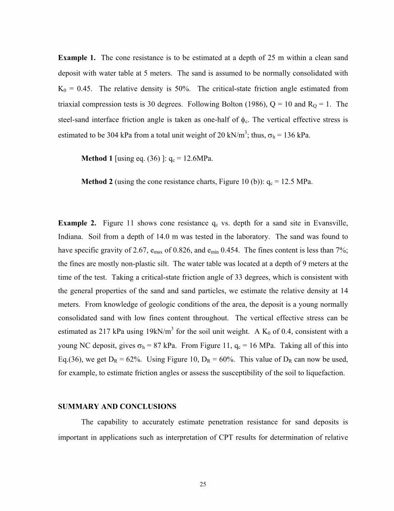
Example 1. The cone resistance is to be estimated at a depth of 25 m within a clean sand

deposit with water table at 5 meters. The sand is assumed to be normally consolidated with

K0 = 0.45. The relative density is 50%. The critical-state friction angle estimated from

triaxial compression tests is 30 degrees. Following Bolton (1986), Q = 10 and RQ = 1. The

steel-sand interface friction angle is taken as one-half of φc. The vertical effective stress is

estimated to be 304 kPa from a total unit weight of 20 kN/m3; thus, σh = 136 kPa.

Method 1 [using eq. (36) ]: qc = 12.6MPa.

Method 2 (using the cone resistance charts, Figure 10 (b)): qc = 12.5 MPa.

Example 2. Figure 11 shows cone resistance qc vs. depth for a sand site in Evansville,

Indiana. Soil from a depth of 14.0 m was tested in the laboratory. The sand was found to

have specific gravity of 2.67, emax of 0.826, and emin 0.454. The fines content is less than 7%;

the fines are mostly non-plastic silt. The water table was located at a depth of 9 meters at the

time of the test. Taking a critical-state friction angle of 33 degrees, which is consistent with

the general properties of the sand and sand particles, we estimate the relative density at 14

meters. From knowledge of geologic conditions of the area, the deposit is a young normally

consolidated sand with low fines content throughout. The vertical effective stress can be

estimated as 217 kPa using 19kN/m3 for the soil unit weight. A K0 of 0.4, consistent with a

young NC deposit, gives σh = 87 kPa. From Figure 11, qc = 16 MPa. Taking all of this into

Eq.(36), we get DR = 62%. Using Figure 10, DR = 60%. This value of DR can now be used,

for example, to estimate friction angles or assess the susceptibility of the soil to liquefaction.

SUMMARY AND CONCLUSIONS

The capability to accurately estimate penetration resistance for sand deposits is

important in applications such as interpretation of CPT results for determination of relative

26

density and stress state, estimaton of friction angles, assessment of soil liquefaction

susceptibility, and prediction of the capacity of pile foundations to support vertical loads.

Calculation of qc can be done relatively simply if linear elasticity and perfect

plasticity can be assumed for the soil. Values for G, ν and φ of a linear-elastic, perfectly

plastic material in terms of the initial relative density and lateral stress were developed. It

was shown that φ-φc is essentially independent of φc. The ratio of plastic radius to cone

penetrometer radius is also essentially independent of φc. The representative friction angle φ

T within the transition zone around a penetrating cone was found to depend on initial density,

initial lateral effective stress and φc.

Summary charts for qc directly in terms of soil state were developed. Another way of

computing qc is to use a single expression that gives qc as a function of the lateral effective

stress σh and the relative density DR. This expression was derived by fitting the results of the

complete analysis over the entire range of relative density and stress states considered in the

paper (0≤ DR ≤ 100% and 22.5 ≤ σh ≤ 450kPa). Example calculations show that two

different methods of estimating qc are easy to apply and give consistent values.

APPENDIX I. REFERENCES

Baldi et al. (1983). "Prova Penetrométrica Stática e Densitá Relativa della Sabbia." XV CIG

Spoleto, Italy.

Baldi et al. (1985). "Laboratory Validation of In-Situ Tests." AGI JubileeVolume. XI

ICSMFE, San Francisco.

Baldi et al. (1986). "Interpretation of CPT's and CPTU's - Second Part: Drained Penetration

of Sands." Fourth International Conf. on Field Instrumentation and In-situ

Measurement, Nanyang Technological Institute, Singapore, 143-156.

Been, K. and Jefferies, M. G. (1985). "A state parameter for sands." Geotechnique, Vol. 35,

No. 2, pp. 99-112.

27

Bellotti, R., Bizzi, G. and Ghionna, V. (1982). "Design, Construction and Use of a

Calibration Chamber." Proc. ESOPT II, Amsterdam, V.2, 439-446.

Bolton, M.D. (1982). A Guide to Soil Mechanics. MacMillan, 439 pp.

Bolton, M. D. (1986). "The Strength and Dilatancy of Sands." Geotechnique 36(1), 65-78.

Bonita, J.A. (2000). The Effects of Vibration on the Penetration Resistance and Pore Water

Pressure in Sands. Dissertation in partial fulfillment of the requirements for the

Ph.D. degree in Civil Engineering, Virginia Polytechnic Institute and State

University, Blacksburg, VA, July 28, 2000.

Collins, I.F., Pender, M.J. and Yan, W. (1992). "Cavity Expansion in Sands under Drained

Loading Conditions." International Journal for Numerical and Analytical Methods

in Geomechanics, 16, 3-23.

Ghionna, V. and Jamiolkowski, M. (1991). "A Critical Apraisal of Calibration Chamber

Testing of Sands." Proc. First International Symposium on Calibration Chamber

Testing (ISOCCT1). Potsdam, New York: Elsevier, A. B. Huang, ed., 13-39.

Hardin, B. and Black, W. (1968). "Shear Modulus and Damping in Soils." J. Soil Mechs.

Found. Div., 94(2), 353-369.

Houlsby, G. T. and Hitchman, R. (1988). "Calibration Chamber Tests of a Cone

Penetrometer in Sand." Geotechnique 38(1), 39-44.

Houlsby, G.T. & Wroth, C.P. 1989. The Influence of Soil Stiffness and Lateral Stress on the

Results of In-Situ Soil Tests. Proc. XII ICSMFE, Rio de Janeiro, Vol. 1: 227-232.

Aug.

Jamiolkowki, M., Ladd, C., Germaine, J., and Lancellotta, R. (1985). "New Developments in

Field and Laboratory Testing of Soils." Proc. XI ICSMFE, San Francisco.

Ishibashi, I. and Zhang, X. (1993). "Unified Dynamic Shear Moduli and Damping Ratios of

Sand and Clay." Soils and Foudnations, 33(1), 182-191.

28

Lee, K.M., Shen, C.K., Leung, D.H.K. Leung, and Mitchell, J.K. (1999). "Effects of

Placement Method on Geotechnical Behavior of Hydraulic Fill Sands." J. Geotech

and Geoenvir. Engrg. 125(10), 832-846.

Lo Presti, D.C.F. (1987). Ph.D. thesis. Politécnico di Torino, Turin, Italy.

Lo Presti, D.C.F., Pedroni, S. and Crippa, V. (1992). "Maximum Dry Density of

Cohesionless Soils by Pluviation and by ASTM D4253-83: a Comparative Study."

Geotechnical Testing Journal 15(2), 180-189.

Mayne, P.W. and Kulhawy, F.H. (1991). "Calibration Chamber Database and Boundary

Effects Correction for CPT Data." Proc. First International Symposium on Calibration

Chamber Testing (ISOCCT1). Potsdam, New York: Elsevier, A. B. Huang, ed., 257-

264.

Mitchell, J. K. (1988). "New Developments in Penetration Tests and Equipment."

Penetration Testing 1988, ISOPT-1, J. De Ruiter, ed., V. 1, 245-261, A.A. Balkema,

Rotterdam.

Miura, S. and Toki, S. (1982), "A Sample Preparation Method and its Effect on Static and

Cyclic Deformation - Strength Properties of Sand", Soils and Foundations, 22(1),

61-77.

Rowe, P. W. (1962). "The stress-dilatancy relation for static equilibrium of an assembly of

particles in contact." Proc., Royal Soc., London, A269, 500-527.

Salgado, R. (1993). "Analysis of Penetration Resistance in Sands," Ph.D. thesis, University

of California, Berkeley, Calif.

Salgado, R., Bandini, P. and Karim, A. (2000). "Shear Strength and Stiffness of Silty Sands."

Journal of Geotechnical and Geoenvironmental Engineering, ASCE, 126(5), 451-462.

Salgado, R., Mitchell, J. K., and Jamiolkowski, M. (1997a). "Cavity Expansion and

Penetration Resistance in Sand." Journal of Geotechnical and Geoenvironmental

Engineering, ASCE, 123(4), 344-354.

29

Salgado, R., Boulanger, R. W., and Mitchell, J. K. (1997b). "Lateral Stress Effects on CPT

Liquefaction Resistance Correlations." Journal of Geotechnical and

Geoenvironmental Engineering, ASCE, 123(8), 726-735.

Salgado, R., Mitchell, J. K., and Jamiolkowski, M. B. (1998). "Chamber Size Effects on

Penetration Resistance Measured in Calibration Chambers." Journal of Geotechnical

and Geoenvironmental Engineering, ASCE, 124(9), Sep., pp. 878-888.

Salgado, R. and Randolph, M.F. (2001). "Analysis of Cavity Expansion in Sand."

International Journal of Geomechanics, 1(2), 175-192.

Schmertmann, J. (1976). "An Updated Correlation between Relative Density DR, and Fugro-

type Electric Cone Bearing qc." Waterways Experimental Station Contract Report

DACW 39-76 M6646.

Vésic, A.S. (1972), "Expansion of Cavities in Infinite Soil Mass." J. Soil Mech. Found. Div.,

ASCE, March, 265-290.

Villet, W. C. B. and Mitchell, J. K. (1981). "Cone Resistance, Relative Density, and Friction

Angle." Proc. ASCE Symposium on Cone Penetration Testing and Experience

(Norris and Holtz, eds.), St. Louis, MO, 178-208.

30

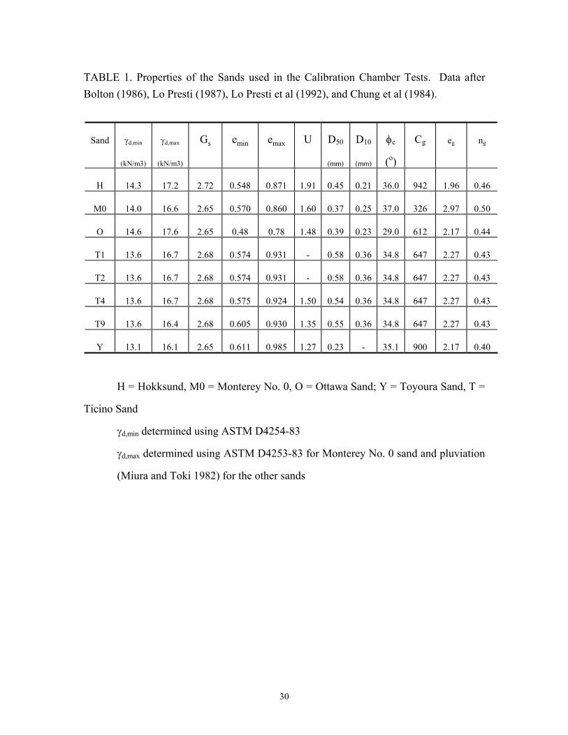
TABLE 1. Properties of the Sands used in the Calibration Chamber Tests. Data after Bolton (1986), Lo Presti (1987), Lo Presti et al (1992), and Chung et al (1984).

Sand γd,min

(kN/m3)

γd,max

(kN/m3)

Gs emin emax U D50

(mm)

D10

(mm)

φc

(o)

Cg eg ng

H 14.3 17.2 2.72 0.548 0.871 1.91 0.45 0.21 36.0 942 1.96 0.46

M0 14.0 16.6 2.65 0.570 0.860 1.60 0.37 0.25 37.0 326 2.97 0.50

O 14.6 17.6 2.65 0.48 0.78 1.48 0.39 0.23 29.0 612 2.17 0.44

T1 13.6 16.7 2.68 0.574 0.931 - 0.58 0.36 34.8 647 2.27 0.43

T2 13.6 16.7 2.68 0.574 0.931 - 0.58 0.36 34.8 647 2.27 0.43

T4 13.6 16.7 2.68 0.575 0.924 1.50 0.54 0.36 34.8 647 2.27 0.43

T9 13.6 16.4 2.68 0.605 0.930 1.35 0.55 0.36 34.8 647 2.27 0.43

Y 13.1 16.1 2.65 0.611 0.985 1.27 0.23 - 35.1 900 2.17 0.40

H = Hokksund, M0 = Monterey No. 0, O = Ottawa Sand; Y = Toyoura Sand, T =

Ticino Sand

γd,min determined using ASTM D4254-83

γd,max determined using ASTM D4253-83 for Monterey No. 0 sand and pluviation

(Miura and Toki 1982) for the other sands

31

32

List of Figures

Figure 1 Cavity expansion: cavity and the plastic and elastic zones.

Figure 2 Equivalent linear shear modulus as function of initial soil state: (a) φc = 29° and (b) φc = 36°.

Figure 3 Equivalent linear friction angle as function of initial soil state: (a) φc = 29°, (b) φc = 33 and (c) φc = 36°.

Figure 4 Ratio of plastic radius to cavity radius when cylindrical cavity limit pressure is reached: (a) φc = 29° and (b) φc = 36°.

Figure 5 Cylindrical cavity limit pressure as a function of initial soil state for a normally-consolidated sand with critical-state friction angle equal to: (a) 29° , (b) 30°, (c) 31°, (d) 32°, (e) 33°, (f) 34°, (g) 35° and (h) 36°.

Figure 6 Assumed slip mechanism for cone penetration in sand.

Figure 7 Transition zone friction angle φT as function of initial soil state: (a) φc = 29˚, (b) φc = 33˚ and (c) φc = 36˚.

Figure 8 Comparison of predicted with measured values of cone resistance for calibration chamber tests on West Kowloon sand (after Lee et al. 1999).

Figure 9 Cone resistance calculated both using CONPOINT with Ticino Sand properties and cone resistance measured in calibration chamber tests on normally, 1-D consolidated samples of Ticino Sand with DR within the 10-20%, 50-60% and 90-100% ranges, performed under BC1 boundary conditions (data after Salgado 1993 and Salgado et al. 1997).

Figure 10 Cone penetration resistance using CONPOINT as a function of initial soil state for a normally-consolidated sand with φc equal to: (a) 29° , (b) 30°, (c) 31°, (d) 32°, (e) 33°, (f) 34°, (g) 35° and (h) 36°.

Figure 11 CPT log from a site in Evansville, Indiana (test performed by Dr. Junhwan Lee).