Strategic Asset Allocation - Determining the Optimal Portfolio
Growth Optimal Portfolio Selection with Short Selling and Leverage 1
Chapter 5
GROWTH OPTIMAL PORTFOLIO SELECTION WITH
SHORT SELLING AND L EVERAGE
Mark Horvath and Andras Urban
Abstract
The growth optimal strategy on non-leveraged, long only markets is the best con-stantly rebalanced portfolio (BCRP), also called log-optimal strategy. We derive opti-mality conditions to frameworks on leverage and short selling, and generalize BCRPby establishing no ruin conditions. Moreover we investigate the strategy and its asymp-totic growth rate from both theoretical and empirical points of view, under memorylessassumption on the underlying process. The empirical performance of the methods isillustrated for NYSE data.
Keywords: growth optimal investment, log-optimal portfolio, BCRP, rebalancing, shortselling, leverage, margin buying, Karush-Kuhn-Tucker, convex optimization, portfolio op-timizationAMS Subject Classification (2010):91A60, 91B06, 91B28, 91B62, 91G10.

2 Mark Horvath and Andras Urban
1. Introduction
Earlier results in the non-parametric statistic, information theory and economic literature(such as Kelly [11], Latane [12], Breiman [2], Markowitz [14], [15], Finkelstein andWhitley [7]) have established optimality criterion for long-only, non-leveraged investment.These results have shown that the market is inefficient, i.e. substantial gainis achievableby rebalancing and predicting market returns based on market’s history.Our aim is to showthat using leverage through margin buying (the act of borrowing money and increasingmarket exposure) yields substantially higher growth rate in the case of memoryless (i.i.d.)assumption over returns. Besides a framework for leveraged investment,we also establishmathematical basis for short selling, i.e. creating negative exposure to asset prices. Shortselling means the process of borrowing assets and selling them immediately, with the obli-gation to rebuy them later.
It can be shown that the optimal asymptotic growth rate on a memoryless market co-incides with that of the best constantly rebalanced portfolio (BCRP). The idea is that on africtionless market the investor can rebalance his portfolio for free at each trading period.Hence asymptotic optimization on a memoryless market means that the growth optimalstrategy will pick the same portfolio vector at each trading period. Strategiesbased onthis observation are called constantly rebalanced portfolios (CRP), while the one with thehighest asymptotic average growth rate is referred to as BCRP. Our results include the gen-eralization of BCRP for margin buying and short selling frameworks.
To allow short and leverage our formulation weaken the constraints on feasible set ofpossible portfolio vectors, thus they are expected to improve performance. Leverage is an-ticipated to have substantial merit in terms of growth rate, while short selling is not expectedto yield much better results. We do not expect increased profits on short CRP strategy,since companies worth to short in our test period should have already defaulted by now.Nonetheless short selling might to yield increased profits in case of markets with memory,since earlier results have shown that the market was inefficient ([8]).
Cover [3] has introduced a gradient based method for optimization of long-only log-optimal portfolios, and gave necessary and sufficient conditions on growth optimal invest-ment in Bell and Cover [19]. We extend these results to short selling and leverage.
Contrary to non-leveraged long only investment in earlier literature, in caseof mar-gin buying and short selling it is easy to default on total initial investment. In thiscaseasymptotic growth rate is minus infinity. By bounding possible market returns, we estab-lish circumstances such that default is impossible. We do this in such a way, that debt andpositions are limited and the investor is always able to satisfy his liabilities selling assets.Restriction of market exposure and amount of debt is in line with the practice of brokeragesand regulators.
Our notation for asset prices and returns are as follows. Consider a market consisting ofd assets. Evolution of prices is represented by a sequence of price vectors s1, s2, . . . ∈ R
d+,
where
sn = (s(1)n , . . . , s(d)n ). (1)
s(j)n denotes the price of thej-th asset at the end of then-th trading period. In order to
apply the usual techniques for time series analysis, we transform the sequence of price
Growth Optimal Portfolio Selection with Short Selling and Leverage 3
vectors{sn} into return vectors:
xn = (x(1)n , . . . , x(d)n ),
where
x(j)n =s(j)n
s(j)n−1
.
Here thej-th componentx(j)n of the return vectorxn denotes the amount obtained by in-vesting unit capital in thej-th asset during then-th trading period.
2. Non-leveraged, long only investment
A representative example of the dynamic portfolio selection in the long only case is theconstantly rebalanced portfolio (CRP), introduced and studied by Kelly [11], Latane [12],Breiman [2], Markowitz [15], Finkelstein and Whitley [7], Mori [16] and Mori and Szekely[17]. For a comprehensive survey, see also Chapters 6 and 15 in Cover and Thomas [4], andChapter 15 in Luenberger [13].
CRP is a self-financing portfolio strategy, rebalancing to the same proportional portfolioin each investment period. This means that the investor neither consumes from, nor depositsnew cash into his account, but reinvests his capital in each trading period.Using this strategythe investor chooses a proportional portfolio vectorb = (b(1), . . . , b(d)), and rebalances hisportfolio after each period to correct the price shifts in the market. This waythe proportionof his wealth invested in each asset is constant at the beginning of trading periods.
The j-th componentb(j) of b denotes the proportion of the investor’s capital investedin assetj. Thus the portfolio vector has nonnegative components that sum up to1. The setof portfolio vectors is denoted by
∆d =
b = (b(1), . . . , b(d)); b(j) ≥ 0,
d∑
j=1
b(j) = 1
. (2)
Let S0 denote the investor’s initial capital. At the beginning of the first trading periodS0b
(j) is invested into assetj, and it results in position sizeS0b(j)x
(j)1 after changes in
market prices. Therefore, at the end of the first trading period the investor’s wealth becomes
S1 = S0
d∑
j=1
b(j)x(j)1 = S0 〈b , x1〉 ,
where〈· , ·〉 denotes inner product. For the second trading periodS1 is the new initialcapital, hence
S2 = S1 〈b , x2〉 = S0 〈b , x1〉 〈b , x2〉 .By induction for trading periodn,
Sn = Sn−1 〈b , xn〉 = S0
n∏
i=1
〈b , xi〉 . (3)

4 Mark Horvath and Andras Urban
Including cash account into the framework is straight forward by assuming
x(j)1 = 1.
The asymptotic average growth rate of this portfolio selection is
W (b) = limn→∞
ln n√Sn = lim
n→∞
1
nlnSn
= limn→∞
(1
nlnS0 +
1
n
n∑
i=1
ln 〈b , xi〉)
= limn→∞
1
n
n∑
i=1
ln 〈b , xi〉 ,
which follows from positivity of〈b , xi〉. This also means that without loss of generalitywe can assume that the initial capitalS0 = 1.
If the market process{Xi} is memoryless, i.e., it is a sequence of i.i.d. random returnvectors, then the optimal CRP strategy is the called the best constantly rebalanced portfolio(BCRP). In case of i.i.d. market processes the asymptotic rate of growth is
W (b) = limn→∞
1
n
n∑
i=1
ln 〈b , Xi〉 = E ln 〈b , X〉 a.s., (4)
given thatE ln 〈b , X〉 is finite, due to strong law of large numbers. We can ensure thisproperty by finiteness of
E lnX(j).
If b(j) ≥ 0 for j = 1, . . . , d, thenE ln 〈b , X〉 is finite, too. This is because for any fixedbwith b(j) > 0 and
E lnX(j) > M,
we have thatE ln b(j)X(j) > ln b(j) +M.
Therefore
E ln 〈b,X〉 = E
{ln
d∑
i=1
b(i)X(i)
}≥ ln b(j) +M > −∞.
Similarly
E ln 〈b , X〉 ≤ E
n∑
j=1
lnX(j)
< ∞.
From (4) it follows that rebalancing to
b∗ ∈ arg max
b∈∆d
W (b),
is an optimal trading strategy, i.e.
W (b∗) ≥ W (b),

Growth Optimal Portfolio Selection with Short Selling and Leverage 5
for anyb ∈∆d. Thus BCRP rebalances tob∗ at the beginning of each trading period.Besides almost sure long term optimality the log-optimal strategy offers other advan-
tages, such as
• The log-optimal strategy is competitively optimal on the short term in the sense that
P(S∗n ≥ S′
n) ≥1/2,
whereS′n is the wealth achieved by any other investment strategy. That is given two
portfolio managers, the manager of a growth optimal portfolio is likely to outperformsthe other (cf. Bell and Cover [19]). This is related to median optimization propertyof log-optimal investment.
• The expected time required to achieve a certain capitalA is minimized by growth op-timal investment in the limit, asA → ∞ (cf. Bell and Cover [19]). It is suspected thatthe probability of reaching a given level of wealth at a given time is also maximizedby the growth optimal portfolio (see Roll [21]).
• Short term expected optimality in the sense that
E(S′n/S
∗n)≤1, (5)
whereS′n is the wealth achieved by any investment strategy (cf. Luenberger [13]).
• The simplicity of growth optimal investment can be seen on the following example.Consider estimation of logarithmic growth on an i.i.d. market:
fX(b) = E ln 〈b,X〉 ≈ 1
n
n∑
i=1
ln 〈b,xi〉 =1
nln
n∏
i=1
〈b,xi〉 =1
nlnSn.
Thus maximizing wealth historically is asymptotically growth optimal. It is impor-tant to note that it is easy to overfit this way given insufficient number of historicalobservations.
• Resemblance to Markowitz type portfolio optimization of semi-log-optimal invest-ment, whereln is estimated by second order Taylor expansion (see [21], [18]). Weinvestigate this later at semi-log-optimal investment.
• According to Fama and MacBeth [1] the growth optimal portfolio with fixed con-sumption is also growth optimal.
• In contrast with many investment frameworks (like quadratic utility optimization ofMarkowitz), the growth optimal framework is non-parametric, and capturesaspectsof higher moments and non-linear comovements of prices distribution.
In the followings we repeat calculations of Bell and Cover in [19]. Our aimis to max-imize asymptotic average rate of growth.W (b) being concave, we minimize the convexobjective function
fX(b) = −W (b) = −E ln 〈b,X〉 . (6)
6 Mark Horvath and Andras Urban
To use Karush-Kuhn-Tucker theorem we establish linear, inequality typeconstraintsover the search space∆d in (2):
−b(i) ≤ 0,
for i = 1, . . . , d, i.e.〈b, ai〉 ≤ 0, (7)
whereai ∈ Rd denotes thei-th unit vector, having−1 at positioni.
Our only equality type constraint is
d∑
j=1
b(j) − 1 = 0,
i.e.〈b, e〉 − 1 = 0, (8)
wheree ∈ Rd, e = (1, 1, . . . , 1).
The partial derivatives of the objective function are
∂fX(b)
∂b(i)= −E
X(i)
〈b,X〉 ,
for i = 1, . . . , d.According to Karush-Kuhn-Tucker theorem ([10]), the portfolio vector b∗ is optimal if
and only if, there are constantsµi ≥ 0 (i = 1, . . . , d) andϑ ∈ R, such that
f ′X(b∗) +
d∑
i=1
µiai + ϑe = 0
andµj 〈b∗, aj〉 = 0,
for j = 1, . . . , d.This means that
−EX(j)
〈b∗,X〉 − µj + ϑ = 0 (9)
andµjb
∗(j) = 0,
for j = 1, . . . , d. Summing up (9) weighted byb∗(j), we obtain:
−E〈b∗,X〉〈b∗,X〉 −
d∑
j=1
µjb∗(j) +
d∑
j=1
ϑb∗(j) = 0,
henceϑ = 1.
We can state the following necessary condition for optimality ofb∗. If
b∗ ∈ arg max
b∈∆d
W (b),
Growth Optimal Portfolio Selection with Short Selling and Leverage 7
then
b∗(j) > 0 =⇒ µj = 0 =⇒ EX(j)
〈b∗,X〉 = 1, (10)
and
b∗(j) = 0 =⇒ µj ≥ 0 =⇒ EX(j)
〈b∗,X〉 ≤ 1. (11)
Note that (5) is a consequence of the latter condition in case ofn = 1 andb = −aj .Because of convexity offX(b) the former conditions are necessary, too. Assume
b∗∈∆d. If for any fixedj = 1, . . . , d either
EX(j)
〈b∗,X〉 = 1 andb∗(j) > 0,
or
EX(j)
〈b∗,X〉 ≤ 1 andb∗(j) = 0,
thenb∗ is optimal. The latter two conditions pose a necessary and sufficient conditiononoptimality of b∗.
Remark 1. In case of anindependent asset, i.e. for somej ∈ 1, . . . , d, X(j) being inde-pendent from the rest of the assets,
b∗(j) = 0 =⇒ EX(j)
〈b∗,X〉 ≤ 1
implies byb∗(j) = 0 thatX(j) is independent of〈b∗,X〉. This means that
b∗(j) = 0 =⇒ EX(j)E
1
〈b∗,X〉 ≤ 1,
therefore
b∗(j) = 0 =⇒ EX(j) ≤ 1
E1
〈b∗,X〉
.
According to Karush-Kuhn-Tucker theorem, for any fixedj = 1, . . . , d either
EX(j)
〈b∗,X〉 = 1 andb∗(j) > 0,
or
EX(j) ≤ 1
E1
〈b∗,X〉
andb∗(j) = 0,
if and only if b∗ is optimalb∗ ∈ arg max
b∈∆d
W (b). (12)
Remark 2. Assume optimal portfoliob∗ for d assets
X = (X(1), X(2), . . . , X(d))

8 Mark Horvath and Andras Urban
is already established. Given a new asset – being independent of our previousd assets – wecan formulate a condition on its inclusion in the new optimal portfoliob
∗∗. If
EX(d+1) <1
E1
〈b∗,X〉
thenb∗∗(d+1) = 0.
This means that, for a new independent asset like the cash, we do not have to do theopti-mization for each asset in the portfolio, and we can reach substantial reduction indimensionof the search for an optimal portfolio.
Remark 3. The same trick can be applied in case ofdependent returns as well. If
EX(d+1)
〈b∗,X〉 < 1 thenb∗∗(d+1) = 0,
which is much simpler to verify then performingoptimization of asymptotic averagegrowth. This condition can be formulated as
EX(d+1)E
1
〈b∗,X〉 + Cov(X(d+1),1
〈b∗,X〉) ≤ 1,
which poses a condition on covariance and expected value of the new asset.
Remark 4. Roll [21] suggested an approximation ofb∗ using
ln z ≈ h(z) = z − 1− 1
2(z − 1)2,
which is the second order Taylor approximation of the functionln z at z = 1. Then thesemi-log-optimal portfolio selection is
b ∈ arg maxb∈∆d
E{h 〈b , X〉}.
Our new objective function is convex:
fX(b) = −E{h 〈b,X〉},
= −E{ 〈b,X〉 − 1− 1
2(〈b,X〉 − 1)2}
= E{− 〈b,X〉+ 1 +1
2(〈b,X〉 − 1)2}
= E{− 〈b,X〉+ 1 +1
2〈b,X〉2 − 〈b,X〉+ 1
2}
= E{12〈b,X〉2 − 2 〈b,X〉+ 3
2}
=1
2〈b,E(XX
T )b〉 − 〈b, 2EX〉+ 3
2
= E
{(1√2〈b,X〉 −
√2)2
− 1
2
}.
Growth Optimal Portfolio Selection with Short Selling and Leverage 9
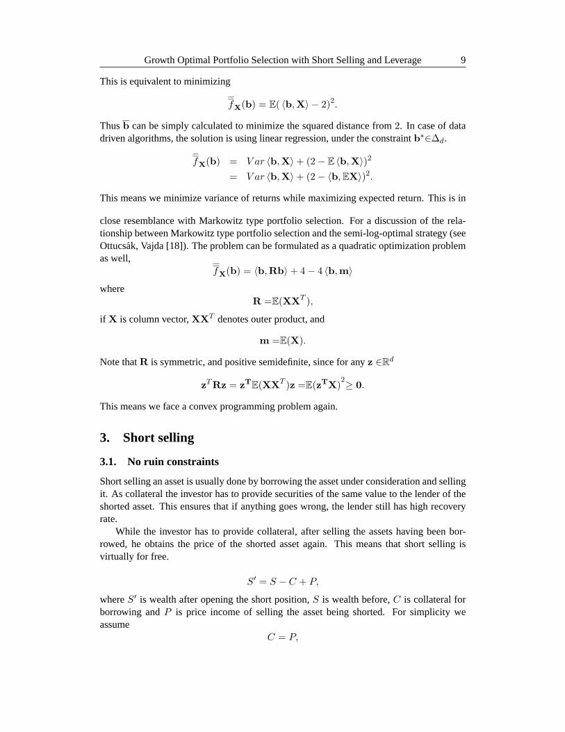
This is equivalent to minimizing
fX(b) = E( 〈b,X〉 − 2)2.
Thusb can be simply calculated to minimize the squared distance from2. In case of datadriven algorithms, the solution is using linear regression, under the constraintb∗∈∆d.
fX(b) = V ar 〈b,X〉+ (2− E 〈b,X〉)2
= V ar 〈b,X〉+ (2− 〈b,EX〉)2.
This means we minimize variance of returns while maximizing expected return. Thisis in
close resemblance with Markowitz type portfolio selection. For a discussion of the rela-tionship between Markowitz type portfolio selection and the semi-log-optimal strategy (seeOttucsak, Vajda [18]). The problem can be formulated as a quadratic optimization problemas well,
fX(b) = 〈b,Rb〉+ 4− 4 〈b,m〉where
R =E(XXT ),
if X is column vector,XXT denotes outer product, and
m =E(X).
Note thatR is symmetric, and positive semidefinite, since for anyz ∈Rd
zTRz = z
TE(XX
T )z =E(zTX)2≥ 0.
This means we face a convex programming problem again.
3. Short selling
3.1. No ruin constraints
Short selling an asset is usually done by borrowing the asset under consideration and sellingit. As collateral the investor has to provide securities of the same value to the lender of theshorted asset. This ensures that if anything goes wrong, the lender still has high recoveryrate.
While the investor has to provide collateral, after selling the assets having been bor-rowed, he obtains the price of the shorted asset again. This means that short selling isvirtually for free.
S′ = S − C + P,
whereS′ is wealth after opening the short position,S is wealth before,C is collateral forborrowing andP is price income of selling the asset being shorted. For simplicity weassume
C = P,
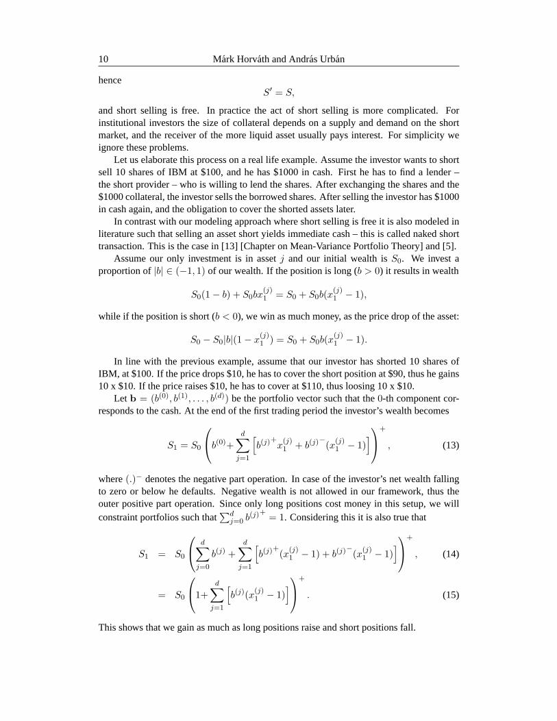
10 Mark Horvath and Andras Urban
henceS′ = S,
and short selling is free. In practice the act of short selling is more complicated. Forinstitutional investors the size of collateral depends on a supply and demandon the shortmarket, and the receiver of the more liquid asset usually pays interest. Forsimplicity weignore these problems.
Let us elaborate this process on a real life example. Assume the investor wants to shortsell 10 shares of IBM at $100, and he has $1000 in cash. First he hasto find a lender –the short provider – who is willing to lend the shares. After exchanging the shares and the$1000 collateral, the investor sells the borrowed shares. After selling the investor has $1000in cash again, and the obligation to cover the shorted assets later.
In contrast with our modeling approach where short selling is free it is alsomodeled inliterature such that selling an asset short yields immediate cash – this is called naked shorttransaction. This is the case in [13] [Chapter on Mean-Variance PortfolioTheory] and [5].
Assume our only investment is in assetj and our initial wealth isS0. We invest aproportion of|b| ∈ (−1, 1) of our wealth. If the position is long (b > 0) it results in wealth
S0(1− b) + S0bx(j)1 = S0 + S0b(x
(j)1 − 1),
while if the position is short (b < 0), we win as much money, as the price drop of the asset:
S0 − S0|b|(1− x(j)1 ) = S0 + S0b(x
(j)1 − 1).
In line with the previous example, assume that our investor has shorted 10 shares ofIBM, at $100. If the price drops $10, he has to cover the short positionat $90, thus he gains10 x $10. If the price raises $10, he has to cover at $110, thus loosing 10 x $10.
Let b = (b(0), b(1), . . . , b(d)) be the portfolio vector such that the0-th component cor-responds to the cash. At the end of the first trading period the investor’swealth becomes
S1 = S0
b(0)+
d∑
j=1
[b(j)
+x(j)1 + b(j)
−(x
(j)1 − 1)
]
+
, (13)
where(.)− denotes the negative part operation. In case of the investor’s net wealth fallingto zero or below he defaults. Negative wealth is not allowed in our framework, thus theouter positive part operation. Since only long positions cost money in this setup, we willconstraint portfolios such that
∑dj=0 b
(j)+ = 1. Considering this it is also true that
S1 = S0
d∑
j=0
b(j) +d∑
j=1
[b(j)
+(x
(j)1 − 1) + b(j)
−(x
(j)1 − 1)
]
+
, (14)
= S0
1+
d∑
j=1
[b(j)(x
(j)1 − 1)
]
+
. (15)
This shows that we gain as much as long positions raise and short positions fall.

Growth Optimal Portfolio Selection with Short Selling and Leverage 11
We can see that short selling is a risky investment, because it is possible to defaulton total initial wealth without the default of any of the the assets in the portfolio.Thepossibility of this would lead to a growth rate of minus infinity, thus we restrict ourmarketaccording to
1−B + δ < x(j)n < 1 +B − δ, j = 1, . . . , d. (16)
Besides aiming at no ruin, the role ofδ > 0 is ensuring that rate of growth is finite for anyportfolio vector (i.e.> −∞).
For the usual stock market daily data, there exist0 < a1 < 1 < a2 < ∞ such that
a1 ≤ x(j)n ≤ a2
for all j = 1, . . . , d, for example,a1 = 0.7 and witha2 = 1.2 (cf. Fernholz [20]). Thus,we can chooseB = 0.3.
Given (15) and (16) it is easy to see that maximal loss that we could sufferisB∑d
j=1 |b(j)|. This value has to be constrained to ensure no ruin.We denote the set of possible portfolio vectors by
∆(−B)d =
b = (b(0), b(1), . . . , b(d)); b(0) ≥ 0,
d∑
j=0
b(j)+= 1, B
d∑
j=1
|b(j)| ≤ 1
. (17)
∑dj=0 b
(j)+ = 1 means that we invest all of our initial wealth into some asset – buying long
– or cash. ByB∑d
j=1 |b(j)| ≤ 1, maximal exposure is limited such that ruin is not possible,
and rate of growth it is finite.b(0) is not included in the latter inequality, since possessingcash does not pose risk. Notice that ifB ≤ 1 then∆d+1 ⊂ ∆
(−B)d , and so the achievable
growth rate with short selling can not be smaller than for long only.According to (15) and (16) we show that ruin is impossible:
1 +d∑
j=1
[b(j)(x
(j)1 − 1)
]> 1+
d∑
j=1
[b(j)
+(1−B + δ − 1) + b(j)
−(1 +B − δ − 1)
]
= 1− (B − δ)d∑
j=1
|b(j)|
≥ δd∑
j=1
|b(j)|.
If∑d
j=1 |b(j)| thenb(0) = 1, hence no ruin. In any other case,δ∑d
j=1 |b(j)| > 0, hence wehave not only ensured no ruin, but also
E ln
1+
d∑
j=1
[b(j)(X
(j)1 − 1)
]
+
> −∞.

12 Mark Horvath and Andras Urban
3.2. Optimality condition for short selling with cash account
A problem with∆(−B)d is its non-convexity. To see this consider
b1 = (0, 1) ∈ ∆(−1)1 ,
b2 = (1,−1/2) ∈ ∆(−1)1 ,
withb1 + b2
2= (1/2, 1/4) /∈ ∆
(−1)1 .
This means we can not simply apply Karush-Kuhn-Tucker theorem over∆(−B)d .
Given cash balance, we can transform our non-convex∆(−B)d to a convex region∆(−B)
d ,where application of our tools established in long only investment becomes feasible. Thenew set of possible portfolio vectors is a convex region:
∆(−B)d =
b = (b(0+), b(1+), b(1−), . . . , b(d+), b(d−)) ∈ R
+02d+1
;d∑
j=0
b(j+) = 1, Bd∑
j=1
(b(j+)+b(j−)) ≤ 1
.
Mapping from∆(−B)d to ∆
(−B)d happens by
b = (b(0), (b(1))+, |(b(1))−|, . . . , (b(d))+, |(b(d))−|). (18)
(13) implies that
S1 = S0
b(0)+
d∑
j=1
[b(j+)x
(j)1 + b(j−)(1− x
(j)1 )]
+
,
thus in line with the portfolio vector being transformed we transform the marketvector too
X = (1, X(1), 1−X(1), . . . , X(d), 1−X(d)),
so thatS1 = S0
⟨b, X
⟩.
To use Karush-Kuhn-Tucker theorem we enumerate linear, inequality type constraintsover the search space
Bd∑
j=1
(b(j+)+b(j−)) ≤ 1,
and
b(0+) ≥ 0, b(i+) ≥ 0, b(i−) ≥ 0,
for i = 1, . . . , d. Our only equality type constraint is
d∑
j=0
b(j+) = 1.
Growth Optimal Portfolio Selection with Short Selling and Leverage 13
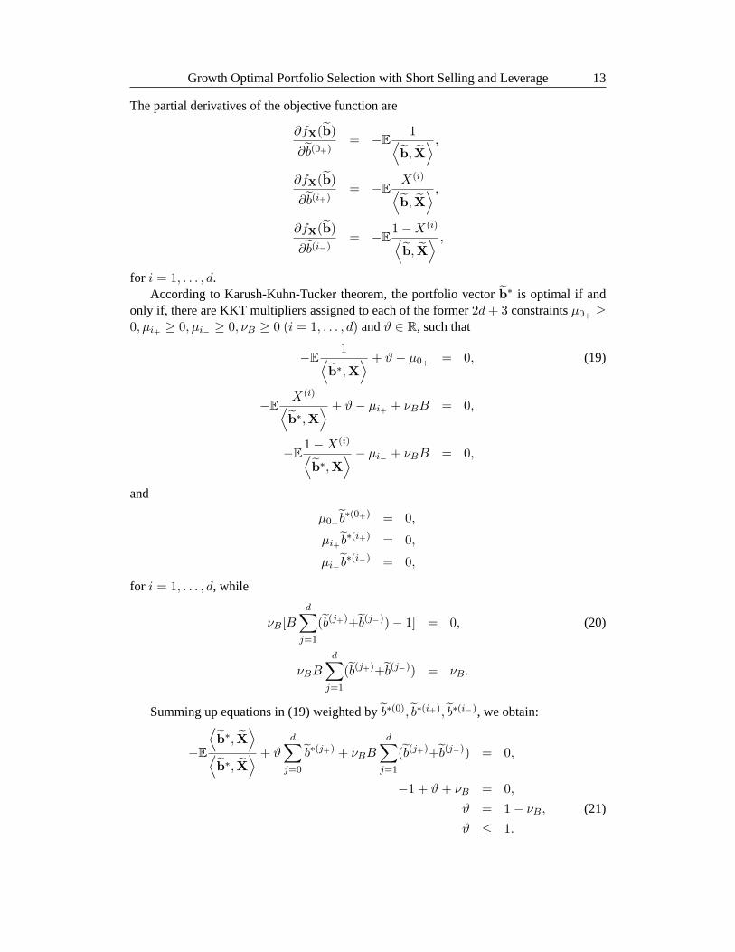
The partial derivatives of the objective function are
∂fX(b)
∂b(0+)= −E
1⟨b, X
⟩ ,
∂fX(b)
∂b(i+)= −E
X(i)
⟨b, X
⟩ ,
∂fX(b)
∂b(i−)= −E
1−X(i)
⟨b, X
⟩ ,
for i = 1, . . . , d.According to Karush-Kuhn-Tucker theorem, the portfolio vectorb
∗ is optimal if andonly if, there are KKT multipliers assigned to each of the former2d+ 3 constraintsµ0+ ≥0, µi+ ≥ 0, µi− ≥ 0, νB ≥ 0 (i = 1, . . . , d) andϑ ∈ R, such that
−E1⟨
b∗,X⟩ + ϑ− µ0+ = 0, (19)
−EX(i)
⟨b∗,X
⟩ + ϑ− µi+ + νBB = 0,
−E1−X(i)
⟨b∗,X
⟩ − µi− + νBB = 0,
and
µ0+ b∗(0+) = 0,
µi+ b∗(i+) = 0,
µi− b∗(i−) = 0,
for i = 1, . . . , d, while
νB[Bd∑
j=1
(b(j+)+b(j−))− 1] = 0, (20)
νBBd∑
j=1
(b(j+)+b(j−)) = νB.
Summing up equations in (19) weighted byb∗(0), b∗(i+), b∗(i−), we obtain:
−E
⟨b∗, X
⟩
⟨b∗, X
⟩ + ϑd∑
j=0
b∗(j+) + νBBd∑
j=1
(b(j+)+b(j−)) = 0,
−1 + ϑ+ νB = 0,
ϑ = 1− νB, (21)
ϑ ≤ 1.

14 Mark Horvath and Andras Urban
In case ofB∑d
j=1(b(j+)+b(j−)) < 1, because of (20) and (21) we have that
νB = 0, henceϑ = 1.
This implies
−E1⟨
b∗, X⟩ + ϑ− µ0+ = 0,
−EX(i)
⟨b∗, X
⟩ + ϑ− µi+ = 0,
−E1−X(i)
⟨b∗, X
⟩ − µi− = 0.
These equations result in the following additional properties
b∗(0+) > 0 =⇒ µ0+ = 0 =⇒ E1⟨
b∗, X⟩ = 1,
b∗(0+) = 0 =⇒ µ0+ ≥ 0 =⇒ E1⟨
b∗, X⟩ ≤ 1,
and
b∗(i+) > 0 =⇒ µi+ = 0 =⇒ EX(i)
⟨b∗, X
⟩ = 1,
b∗(i+) = 0 =⇒ µi+ ≥ 0 =⇒ EX(i)
⟨b∗, X
⟩ ≤ 1,
and
b∗(i−) > 0 =⇒ µi− = 0 =⇒ E1−X(i)
⟨b∗, X
⟩ = 0,
b∗(i−) = 0 =⇒ µi− ≥ 0 =⇒ E1−X(i)
⟨b∗, X
⟩ ≤ 0.
We transform the vectorb∗ to the vectorb∗ such that
b∗(i) = b∗(i+) − b∗(i−)
(i = 1, . . . , d), while
b∗(0) = b∗(0) +d∑
i=1
min{b∗(i+), b∗(i−)}.

Growth Optimal Portfolio Selection with Short Selling and Leverage 15
This wayd∑
j=1
|b∗(j)| = 1,
and we have the same exposure withb∗ as withb.
Due to the simple mapping (18), with regard to the original portfolio vectorb∗ this
means
b∗(0) > 0 =⇒ E1⟨
b∗, X⟩ = 1, (22)
b∗(0) = 0 =⇒ E1⟨
b∗, X⟩ ≤ 1.
Also
b∗(i) > 0 =⇒ EX(i)
⟨b∗, X
⟩ = 1 and E1−X(i)
⟨b∗, X
⟩ ≤ 0,
which is equivalent to
E1⟨
b∗, X⟩ ≤ E
X(i)
⟨b∗, X
⟩ = 1,
and
b∗(i) = 0 =⇒ EX(i)
⟨b∗, X
⟩ ≤ 1 and E1−X(i)
⟨b∗, X
⟩ ≤ 0,
which is equivalent to
E1⟨
b∗, X⟩ ≤ E
X(i)
⟨b∗, X
⟩ ≤ 1,
and
b∗(i) < 0 =⇒ EX(i)
⟨b∗, X
⟩ ≤ 1 and E1−X(i)
⟨b∗, X
⟩ = 0,
which is equivalent to
E1⟨
b∗, X⟩ = E
X(i)
⟨b∗, X
⟩ ≤ 1.
16 Mark Horvath and Andras Urban
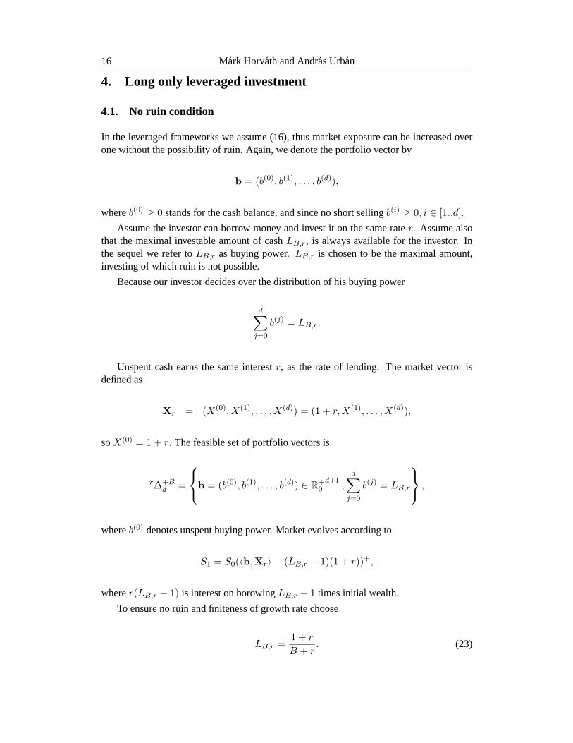
4. Long only leveraged investment
4.1. No ruin condition
In the leveraged frameworks we assume (16), thus market exposure can be increased overone without the possibility of ruin. Again, we denote the portfolio vector by
b = (b(0), b(1), . . . , b(d)),
whereb(0) ≥ 0 stands for the cash balance, and since no short sellingb(i) ≥ 0, i ∈ [1..d].
Assume the investor can borrow money and invest it on the same rater. Assume alsothat the maximal investable amount of cashLB,r, is always available for the investor. Inthe sequel we refer toLB,r as buying power.LB,r is chosen to be the maximal amount,investing of which ruin is not possible.
Because our investor decides over the distribution of his buying power
d∑
j=0
b(j) = LB,r.
Unspent cash earns the same interestr, as the rate of lending. The market vector isdefined as
Xr = (X(0), X(1), . . . , X(d)) = (1 + r,X(1), . . . , X(d)),
soX(0) = 1 + r. The feasible set of portfolio vectors is
r∆+Bd =
b = (b(0), b(1), . . . , b(d)) ∈ R
+0d+1
,d∑
j=0
b(j) = LB,r
,
whereb(0) denotes unspent buying power. Market evolves according to
S1 = S0(〈b,Xr〉 − (LB,r − 1)(1 + r))+,
wherer(LB,r − 1) is interest on borowingLB,r − 1 times initial wealth.
To ensure no ruin and finiteness of growth rate choose
LB,r =1 + r
B + r. (23)
Growth Optimal Portfolio Selection with Short Selling and Leverage 17
This ensures that ruin is not possible:
〈b,Xr〉 − (LB,r − 1)(1 + r)
=d∑
j=0
b(j)X(j) − (LB,r − 1)(1 + r)
= b(0)(1 + r) +d∑
j=1
b(j)X(j) − (LB,r − 1)(1 + r)
> b(0)(1 + r) +d∑
i=1
b(j)(1−B + δ)− (LB,r − 1)(1 + r)
= b(0)(1 + r) + (LB,r − b(0))(1−B + δ)− (LB,r − 1)(1 + r)
= b(0)(r +B − δ)− LB,r(B − δ + r) + 1 + r
≥ − 1 + r
B + r(B − δ + r) + 1 + r
= δ1 + r
B + r.
4.2. Karush-Kuhn-Tucker characterization
Our objective function, the negative of asymptotic rate of growth is
f+BXr
(b) = −E ln(〈b,Xr〉 − (LB,r − 1)(1 + r)).
The linear inequality type constraints are as follows:
−b(i) ≤ 0,
for i = 0 . . . d, while our only equality type constraint is
d∑
j=0
b(j) − LB,r = 0.
The partial derivatives of the optimized function are
∂f+BXr
(b)
∂b(i)= −E
X(i)
〈b,Xr〉 − (LB,r − 1)(1 + r).
According to the Karush-Kuhn-Tucker necessary and sufficient theorem, a portfoliovectorb∗, is optimal if and only if there are KKT multipliersµj ≥ 0 (j = 0 . . . d) andϑ ∈ R, such that
−EX(j)
〈b∗,Xr〉 − (LB,r − 1)(1 + r)− µj + ϑ = 0 (24)
andµjb
∗(j) = 0,

18 Mark Horvath and Andras Urban
for j = 0 . . . d. Summing up (24) weighted byb∗(j) we obtain:
−E〈b∗,Xr〉
〈b∗,Xr〉 − (LB,r − 1)(1 + r)−
d∑
j=0
µjb∗(j) +
d∑
j=0
b∗(j)ϑ = 0,
1 + E(LB,r − 1)(1 + r)
〈b∗,Xr〉 − (LB,r − 1)(1 + r)= LB,rϑ,
1
LB,r
+(LB,r − 1)(1 + r)
LB,r
E1
〈b∗,Xr〉 − (LB,r − 1)(1 + r)= ϑ. (25)
This means that
b∗(j) > 0 =⇒ µj = 0 =⇒ EX(j)
〈b∗,Xr〉 − (LB,r − 1)(1 + r)= ϑ, (26)
and
b∗(j) = 0 =⇒ EX(j)
〈b∗,Xr〉 − (LB,r − 1)(1 + r)≤ ϑ.
For the cash account this means
b∗(0) > 0 =⇒ µj = 0 =⇒ E1 + r
〈b∗,Xr〉 − (LB,r − 1)(1 + r)= ϑ, (27)
and
b∗(0) = 0 =⇒ E1 + r
〈b∗,Xr〉 − (LB,r − 1)(1 + r)≤ ϑ.
5. Short selling and leverage
For this case we need to use both tricks of the previos sections. The marketevolves accord-ing to
S1 = S0
b(0)(1 + r)+
d∑
j=1
[b(j)
+x(j)1 + b(j)
−(x
(j)1 − 1)
]− (LB,r − 1)(1 + r)
+
,
(28)over the non-convex region
r∆±Bd =
b = (b(0), b(1), b(2), . . . , b(d));
d∑
j=0
|b(j)| = LB,r
,
whereLB,r is the buying power defined in (23), andb(0) denotes unspent buying power.Again, one can check that the choice ofLB,r ensures no ruin and finiteness of growth rate.
With the help of our techniqe developed in the short selling framework, we convert tothe following convex region:
r∆±Bd =
b = (b(0+), b(1+), b(1−), . . . , b(d+), b(d−)) ∈ R
+02d+1
; b(0+) +
d∑
j=1
(b(j+) + b(j−)) = LB,r
Growth Optimal Portfolio Selection with Short Selling and Leverage 19
such that
b = (b(0), b(1+), b(1−) . . . , b(d+), b(d−)) = (b(0), b(1)+, |b(1)−|, . . . , b(d)+, |b(d)−|).
Similarly to the short selling case we introduce the transformed return vector.Given
X = (X(1), . . . , X(d)),
we introduce
X±r = (1 + r,X(1), 2−X(1) + r, . . . , X(d), 2−X(d) + r).
We introducer in the terms2 − X(i) + r, since short selling is free, hence buying powerspent on short positions still earns interest. We use2 −X(i) + r instead of1 −X(i) + r,since while short selling is actually free, it still limits our buying power.
Beacause ofr∆±Bd = r∆+B
2d , we can easily apply (26) and (27), hence
b∗(0) > 0 =⇒ E1 + r⟨
b∗,X±r
⟩− (LB,r − 1)(1 + r)
= ϑ,
b∗(0) = 0 =⇒ E1 + r⟨
b∗,X±r
⟩− (LB,r − 1)(1 + r)
≤ ϑ,
whereϑ is defined by (25) withXr = X±r in place, and
b∗(i) > 0 =⇒
EX(i)
⟨b∗,X±r
⟩− (LB,r − 1)(1 + r)
= ϑ,
E2−X(i) + r⟨
b∗,X±r
⟩− (LB,r − 1)(1 + r)
≤ ϑ
and
b∗(i) = 0 =⇒
EX(i)
⟨b∗,X±r
⟩− (LB,r − 1)(1 + r)
≤ ϑ,
E2−X(i) + r⟨
b∗,X±r
⟩− (LB,r − 1)(1 + r)
≤ ϑ
and
b∗(i) < 0 =⇒
EX(i)
⟨b∗,X±r
⟩− (LB,r − 1)(1 + r)
≤ ϑ,
E2−X(i) + r⟨
b∗,X±r
⟩− (LB,r − 1)(1 + r)
= ϑ.
Note, that in the special case ofLB,r = 1, we haveϑ = 1 because of (25).
20 Mark Horvath and Andras Urban
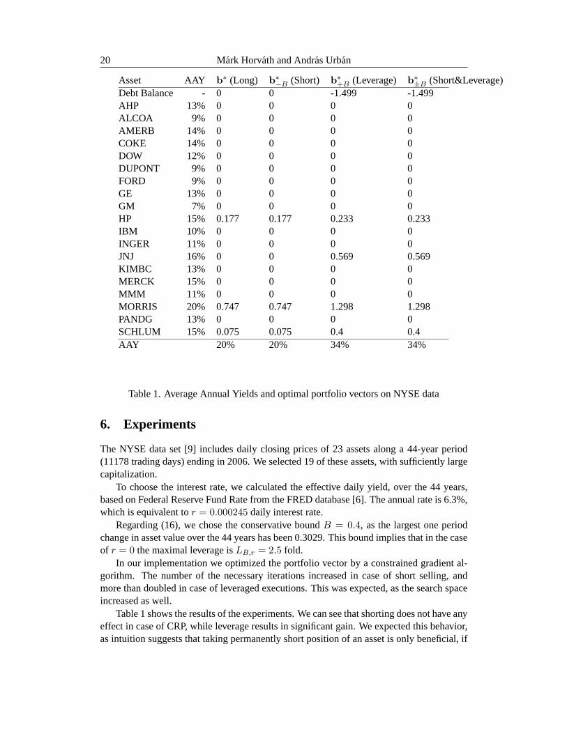
Asset AAY b∗ (Long) b
∗−B (Short) b
∗+B (Leverage) b
∗±B (Short&Leverage)
Debt Balance - 0 0 -1.499 -1.499AHP 13% 0 0 0 0ALCOA 9% 0 0 0 0AMERB 14% 0 0 0 0COKE 14% 0 0 0 0DOW 12% 0 0 0 0DUPONT 9% 0 0 0 0FORD 9% 0 0 0 0GE 13% 0 0 0 0GM 7% 0 0 0 0HP 15% 0.177 0.177 0.233 0.233IBM 10% 0 0 0 0INGER 11% 0 0 0 0JNJ 16% 0 0 0.569 0.569KIMBC 13% 0 0 0 0MERCK 15% 0 0 0 0MMM 11% 0 0 0 0MORRIS 20% 0.747 0.747 1.298 1.298PANDG 13% 0 0 0 0SCHLUM 15% 0.075 0.075 0.4 0.4AAY 20% 20% 34% 34%
Table 1. Average Annual Yields and optimal portfolio vectors on NYSE data
6. Experiments
The NYSE data set [9] includes daily closing prices of 23 assets along a 44-year period(11178 trading days) ending in 2006. We selected 19 of these assets, withsufficiently largecapitalization.
To choose the interest rate, we calculated the effective daily yield, over the 44 years,based on Federal Reserve Fund Rate from the FRED database [6]. The annual rate is 6.3%,which is equivalent tor = 0.000245 daily interest rate.
Regarding (16), we chose the conservative boundB = 0.4, as the largest one periodchange in asset value over the 44 years has been 0.3029. This bound implies that in the caseof r = 0 the maximal leverage isLB,r = 2.5 fold.
In our implementation we optimized the portfolio vector by a constrained gradiental-gorithm. The number of the necessary iterations increased in case of short selling, andmore than doubled in case of leveraged executions. This was expected, as the search spaceincreased as well.
Table 1 shows the results of the experiments. We can see that shorting doesnot have anyeffect in case of CRP, while leverage results in significant gain. We expected this behavior,as intuition suggests that taking permanently short position of an asset is onlybeneficial, if
Growth Optimal Portfolio Selection with Short Selling and Leverage 21
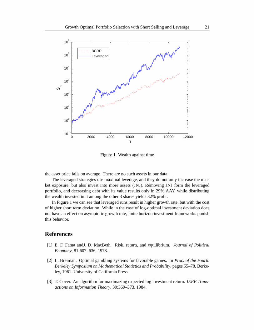
0 2000 4000 6000 8000 10000 1200010
−1
100
101
102
103
104
105
106
n
Sn
BCRPLeveraged
Figure 1. Wealth against time
the asset price falls on average. There are no such assets in our data.The leveraged strategies use maximal leverage, and they do not only increase the mar-
ket exposure, but also invest into more assets (JNJ). Removing JNJ form the leveragedportfolio, and decreasing debt with its value results only in 29% AAY, while distributingthe wealth invested in it among the other 3 shares yields 32% profit.
In Figure 1 we can see that leveraged runs result in higher growth rate,but with the costof higher short term deviation. While in the case of log-optimal investment deviation doesnot have an effect on asymptotic growth rate, finite horizon investment frameworks punishthis behavior.
References
[1] E. F. Fama andJ. D. MacBeth. Risk, return, and equilibrium.Journal of PoliticalEconomy, 81:607–636, 1973.
[2] L. Breiman. Optimal gambling systems for favorable games. InProc. of the FourthBerkeley Symposium on Mathematical Statistics and Probability, pages 65–78, Berke-ley, 1961. University of California Press.
[3] T. Cover. An algorithm for maximazing expected log investment return.IEEE Trans-actions on Information Theory, 30:369–373, 1984.

22 Mark Horvath and Andras Urban
[4] T. Cover and J. A. Thomas.Elements of Information Theory. Wiley, New York, 1991.
[5] T.M. Cover and E. Ordentlich. Universal portfolios with short salesand margin. InProceedings of IEEE International Symposium on Information Theory, June 1998.
[6] FRED Data. Federal reserve fund rate.http://research.stlouisfed.org/fred2/series/FEDFUNDS?cid=118.
[7] M. Finkelstein and R. Whitley. Optimal strategies for repeated games.Advances inApplied Probability, 13:415–428, 1981.
[8] L. Gyorf, G.Lugosi, and F.Udina. Nonparametric kernel based sequential investmentstrategies.Mathematical Finance, 16:337–357, 2006.
[9] L. Gyorfi. Nyse data sets at the log-optimal portfolio homepage.www.szit.bme.hu/∼oti/portfolio.
[10] A. W. H. W. Kuhn andTucker. Nonlinear programming. InProceedings of 2nd Berke-ley Symposium, pages 481–492, Berkeley, California, 1951. University of CaliforniaPress.
[11] J.L. Kelly. A new interpretation of information rate.Bell System Technical Journal,35:917–926, 1956.
[12] H.A. Latane. Criteria for choice among risky ventures.Journal of Political Economy,38:145–155, 1959.
[13] D. G. Luenberger.Investment Science. Oxford University Press, 1998.
[14] H. Markowitz. Portfolio selection.Journal of Finance, 7(1):77–91, 1952.
[15] H. Markowitz. Investment for the long run: New evidence for an oldrule. Journal ofFinance, 31(5):1273–1286, 1976.
[16] T. F. Mri. On favourable stochastic games.Annales Univ. Sci. Budapest. R. Etvs Nom.,Sect. Comput, 3:99–103, 1982.
[17] T. F. Mri and G. J. Szkely. How to win if you can? InProc. Colloquia MathematicaSocietatis Jnos Bolyai 36. Limit Theorems in Probability and Statistics, pages 791–806, 1982.
[18] Gy. Ottucsak and I. Vajda. An asymptotic analysis of the mean-variance portfolioselection.Statistics & Decisions, 25:63–88, 2007.
[19] T. M. Cover R. M. Bell. Competitive optimality of logarithmic investment.Bell. Syst.Tech. J., 27:446–472, 1948.
[20] E. R.Fernholz.Stochastic Portfolio Theory. Springer, New York, 2000.
[21] R. Roll. Evidence on the ”growth-optimum” model.The Journal of Finance, 28:551–566, 1973.