RETURN FORECASTS AND OPTIMAL PORTFOLIO CONSTRUCTION

RETURN FORECASTS AND OPTIMAL PORTFOLIOCONSTRUCTION: A QUANTILE REGRESSION APPROACH

LINGJIE MA AND LARRY POHLMAN

Abstract. In finance, there is growing interest in quantile regression with theparticular focus on value at risk and copula models. In this paper, we first presenta general interpretation of quantile regression in the financial market. We thenexplore the full distributional impact of factors on returns of securities, and find thatfactor effects vary substantially across quantiles of returns. Utilizing distributionalinformation from quantile regression models, we propose two general methods for thereturn forecasting and portfolio construction. We show that under mild conditionsthese new methods provide more accurate forecasts and potentially more value-added portfolios than the classical conditional mean method.

1. introduction

There is intensive research on the return forecasts for securities, and most of ithas focused on the conditional mean estimation strategy. The classical least squaresmethods and maximum likelihood estimator provide attractive methods of estimationfor Gaussian linear equation models with additive errors. However, these methodsoffer only a conditional mean view of the causal relationship, implicitly imposingquite restrictive location-shift assumptions on the way that covariates are allowed toinfluence the conditional distributions of the response variables. Quantile regressionmethods seek to broaden this view, offering a more complete characterization of thestochastic relationship among variables and providing more robust, and consequentlymore efficient, estimates in some non-Gaussian settings.

Since the seminal paper of Koenker and Bassett (1978), quantile regression hasgradually become a complimentary approach for the traditional conditional meanestimation methods. However, in the financial markets, quantile regression has notbeen employed until quite recently. Most of applications of quantile regression infinance have been focused on conditional value at risk models. Engle and Manganelli(2002) have elegantly laid out the natural interpretation of VaR models as the con-cept of quantile regression and considered the application of quantile regression toa nonlinear autoregressive VaR model. Giacomini and Komunjer (2002) proposed aWald-type test to compare different forecasts resulted from the qunatile regression

Version: December 19, 2005. This is the very preliminary version. Please do not cite without theauthors’ authorization. We thank Roger Koenker for comments. Contact information: Lingjie Ma,PanAgora Asset Management, [email protected].

1

2 Return Forecasts and Optimal Portfolio Construction

for VaR models. Chen and Chen (2003) carried out some empirical comparisons andfound that VaR calculations with the quantile regression approach outperform thosewith the variance-covariance approach, and the advantages of the quantile regressionapproach are more obvious in calculating VaRs if the holding periods are longer. Inaddition to the application of quantile regression to VaR models, Bassett and Chen(2001) analyzed the portfolio management styles based on the attribution of returnsusing a quantile regression approach. Barnes and Hughes (2002) applied the quan-tile regression to explore efficacy of the CAPM hypothesis over the distribution ofreturns. Besides the application of quantile regrssion in equity models, another lineof the application is in the fixed income area, where binary quantile regression isemployed to predict the default probability. For the theoretical exploration of binaryquantile regression and applications in the fixed income markets, see Kordas (2002)and Kordas (2004).

While the current literature of quantile gression in finance has focused on risk (VaRmodel) or ex-post analysis of return, in this paper we focus on the return side along theline of forecasting and portfolio construction. We first provide a general interpretationof the quantile regression for not only the risk side but the return side as well. Wethen employ this new statistical methodology to explore the distributional effects offactors on the response of equity models. We introduce two general strategies toillustrate how the distributional information can be utilized to construct an optimalportfolio and show that the portfolio resulting from the distributional estimationmethod outperforms the portfolio constructed based on the classical conditional meanestimation methods.

Section 2 presents a brief review of equity models with an emphasis on the ap-plication of quantile regression methods to equity models. Section 3 describes thequantile regression method through a detailed algorithm and examples. Section 4introduces a general interpretation of quantile regression in equity models as wellas advantages and challenges compared to the traditional methods. Section 5 pro-poses two approaches for the construction of optimal portfolio using the distributionalinformation. Section 6 concludes.

2. literature review

One question has remained central in financial markets: “Is it possible to forecastthe return of securities?” Understanding of the financial markets has been advancedby numerous authors including (but not limited to) Sharpe (1964, CAPM), Famaand French (1992, three-factor model), Lakonishok (1988, 1992, behaviour finance).Through the advance of statistic developments and new technologies, the ability toforecast returns has been greatly enhanced. A typical quantitative approach forreturn forecasting is to build a linear or non linear model based on a combinationof valuation, technical, and expectational factors and apply various conditional meanversions such as least squares methods for the estimation.

Lingjie Ma and Larry Pohlman 3

Indeed, applying the standard conditional mean estimation strategy to a multi-factor model across a diverse range of stocks is a popular approach to ascertain secu-rities’ return appeal. However, by treating different securities as the same, the aboveapproach forces returns of all securities to have the homogeneous mean-reversion be-havior. This mean treatment effect (MTE) view of the factor effect is valid under theextemely strong condition, i.e., the average marginal effect of a factor does not varyacross the size of the factor and returns. However, we know that different securitiesmay have different response for the exposure to the same factor. Thus, the MTE viewis apparently not able to capture such characteristics of factor effects.1 Realizing thatthe factor effects are not constant across securities, some studies such as Barnes andHughes (2002) have pointed out that an estimate of a distributional effect would bepreferred. Quantile regression is a natural tool to accomplish such a task.

A primary example of the growing interest for quantile regression in finance is in thecontext of risk management, as witnessed by the literature on Value at Risk. This isnot a coincidence. Since VaR is simply a particular quantile of future portfolio valuesconditional on current information, the quantile regression is a natural tool to tacklesuch a problem. Engle and Manganelli (1999) were among the first to consider thequantile regression for the VaR model. They construct a conditional autoregressivevalue at risk model (CAViaR), and employ quantile regression for the estimation. Toevaluate the goodness of fit for the estimated results, they also propose a test based onthe idea in Chernozhukov (1999). Their applications to real data suggested that thetails follow different behavior from the middle of the distribution, which contradictsthe assumption behind GARCH and RiskMetrics since such approaches implicitly as-sume that the tails follow the same process as the rest of the returns. Following Engleand Manganelli (1999), Giacomini and Komunjer (2002) propose a testing procedurefor the analysis of competing conditional quantile regression forecasts proposed in theliterature for the VaR model. The test is based on the weight assignments for resultsfrom different methods, which is parallel to the encompassing principle in the contextof conditional mean forecasting.2

Recently, Chen and Chen (2003) carried out an empirical study to compare perfor-mances of Nikkei 225 VaR calculations with the quantile regression approach to thosewith the conventional variance-covariance approach. They find that VaR calculationswith quantile regression outperform those with the variance-covariance approach.Furthermore, the advantage of the quantile regression is more significant for longerholding periods. While the empirical results are encouraging, the application to otherequity markets would be very interesting.

In addition to the application in VaR models, there are studies employing quantileregression in other areas of financial market. Barnes and Hughes (2002) employ

1By specifying certain function forms for a factor, the MTE view may reveal some variations offactor effects across different values of factors.

2For the discussion of the encompassing principle in the context of conditional mean forecasting,please see Hendry and Richard (1982), Mizon and Richard (1986) and Diebold (1989).


quantile regression to test whether the conditional CAPM holds at points of thereturn distribution other than the mean. The empirical results of Barnes and Hughes(2002) provide new support for Merton’s (1987) prediction that size and returns arepositively related which is in contrast to many of the empirical findings reported inthe literature. Realizing that it would be a mistake to think a single measure shoulddescribe a portfolio’s style, Bassett and Chen (2001) employ quantile regression tocharacterize the distributional view of portfolio management styles. They find that inthe small cap value estimates, large positive and negative impacts in the tails canceleach other which leaves barely the hint of the conditional mean result.

While the use of quantile regression in various financial fields has enriched theunderstanding of financial market, one great potential would be to apply this newtool to the quantitative investment practice. To the best of our knowledge, there hasbeen no study employing quantile regression for the purpose of return forecast andportfolio construction. As an initial effort on this topic, this paper explores somebasic methods which might be used to link the quantile regression to the portfolioconstruction. We try not to be too specific about the formulation of the model andproperties of the results, but rather provide a general view on how quantile regressioncould be used for better return forecasting and hence portfolio construction.

3. quantile regression: a brief introduction

Why do we need quantile regression? In most cases, the effects of factors onresponse are not constant, but rather vary across the responses. Suppose we wouldlike to know: How does the debt-ratio factor affect a stock’s return at high and lowvalues? By using the conditional mean etimation method, we would come to theresult that in spite of different return levels, the debt ratio will affect the returns ofall securities exactly the same way. However, if there is heterogeneity in the effects,then different strategies are needed to handle such differences.

How do we capture such heteregenous causal effects? To answer this question,consider the following simple linear model:

yi,t = x>i,tβ + ui,t,(3.1)

where yi,t is the return and xi,t is the k-dimension vector of factors of the stock i attime t, i = 1, 2, . . . , N , t = 1, 2, . . . , T . Assume x is independent of u. For simplicity,consider only the cross-section version of (3.1), i.e., t is fixed at only one period. Fornotation convenience, we will hereafter drop the reference to the index t unless it isneeded for clarification.

For the pure location shift model (3.1), under the conditions that ui is i.i.d. andGaussian, the traditional conditional mean estimation strategy would yield consistentand efficient estimates for the constant causal effect of x on y. However, such restric-tive conditions of i.i.d. and Gaussian errors rarely hold in market data. This modelignores the distributional view on how x effects y, or in other words, heterogeneity. It


is usually true that the effect of x on y would not be constant across y. For example,

yi = x>i β + φ(xi, γ)εi;(3.2)

where φ(.) is usually unknown. Note that now ui = φ(xi, γ)εi is not i.i.d. anymoreeven if εi is assumed to be i.i.d. How does the location-scale shift model, (3.2), capturethe causal effects of x on y distributionally?

0.0 0.5 1.0 1.5 2.0

−200

2040

Debt Ratio

Retur

n

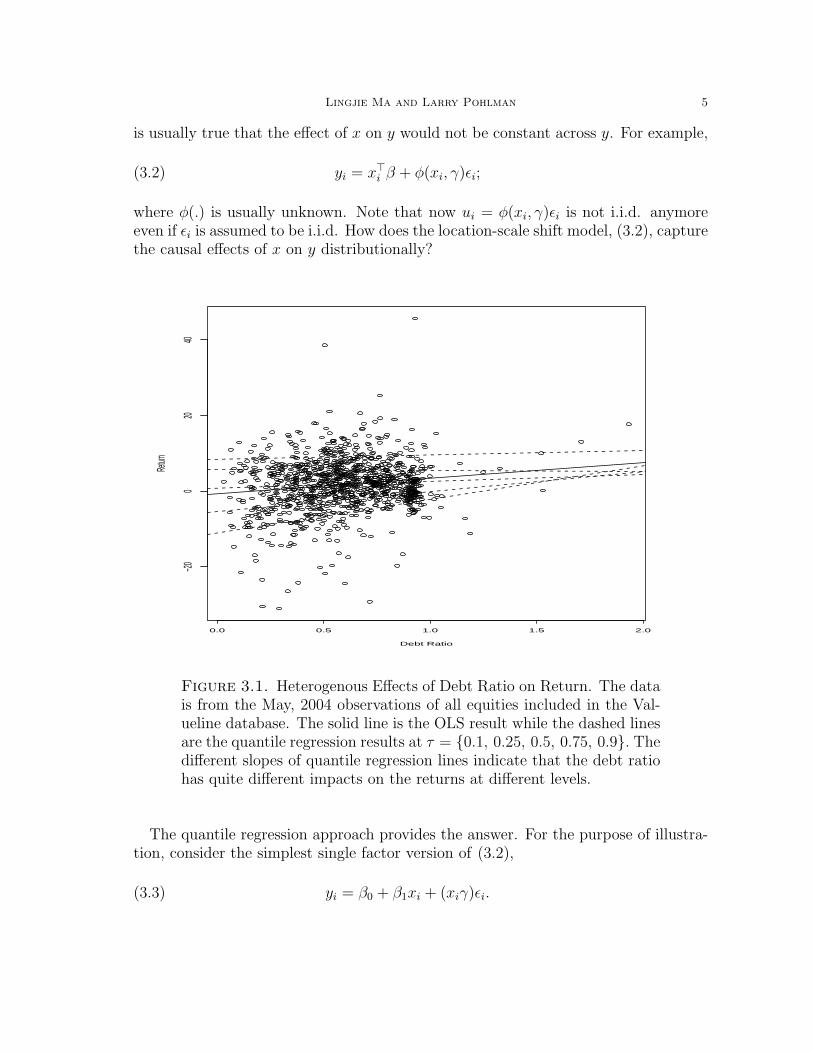
Figure 3.1. Heterogenous Effects of Debt Ratio on Return. The datais from the May, 2004 observations of all equities included in the Val-ueline database. The solid line is the OLS result while the dashed linesare the quantile regression results at τ = 0.1, 0.25, 0.5, 0.75, 0.9. Thedifferent slopes of quantile regression lines indicate that the debt ratiohas quite different impacts on the returns at different levels.

The quantile regression approach provides the answer. For the purpose of illustra-tion, consider the simplest single factor version of (3.2),

yi = β0 + β1xi + (xiγ)εi.(3.3)


0.2 0.4 0.6 0.8

−20

24

68

10

tau

Debt r

atio eff

ect−−

OLS

0.2 0.4 0.6 0.8

−20

24

68

10

tau

Debt r

atio eff

ect−−

QR

o

o

o

o

o

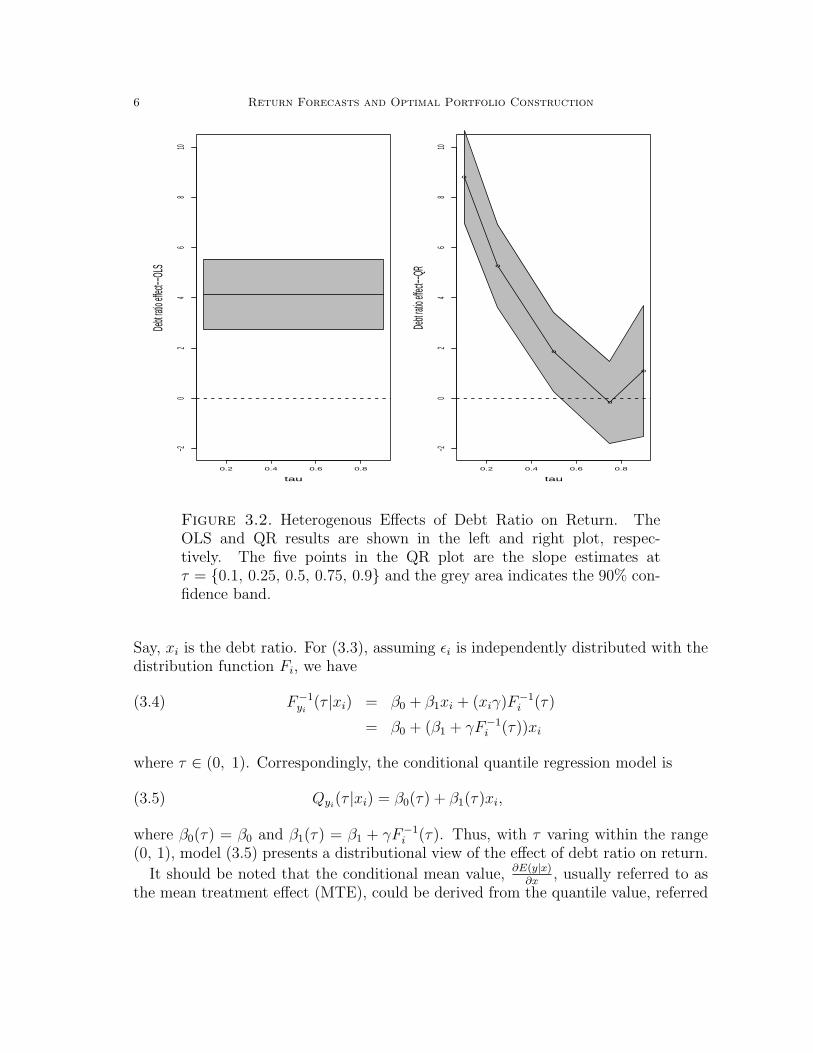
Figure 3.2. Heterogenous Effects of Debt Ratio on Return. TheOLS and QR results are shown in the left and right plot, respec-tively. The five points in the QR plot are the slope estimates atτ = 0.1, 0.25, 0.5, 0.75, 0.9 and the grey area indicates the 90% con-fidence band.

Say, xi is the debt ratio. For (3.3), assuming εi is independently distributed with thedistribution function Fi, we have

F−1yi

(τ |xi) = β0 + β1xi + (xiγ)F−1i (τ)(3.4)

= β0 + (β1 + γF−1i (τ))xi

where τ ∈ (0, 1). Correspondingly, the conditional quantile regression model is

Qyi(τ |xi) = β0(τ) + β1(τ)xi,(3.5)

where β0(τ) = β0 and β1(τ) = β1 + γF−1i (τ). Thus, with τ varing within the range

(0, 1), model (3.5) presents a distributional view of the effect of debt ratio on return.

It should be noted that the conditional mean value, ∂E(y|x)∂x

, usually referred to asthe mean treatment effect (MTE), could be derived from the quantile value, referred


to as the quantile treatment effect (QTE),

MTE =

∫ 1

0

β(t)d t = β1 + γE(ε) = β1 + uε.

In particular, if ε is mean zero, then MTE is the classical conditional mean value, β1.This relationship between MTE and QTE suggests that QTE is the decomposition ofMTE and thus provides a full picture view on the causal effects. Note that the MTEin models with pure location shift is exactly what would be estimated by the leastsquares method.

The above point is illustrated vividly in Figure 3.1–3.2, where the effects of debt ra-tio on returns are explored by using both the OLS and QR methods. Figure 3.1, whichis a scatter plot with slopes obtained from OLS and QR at τ = 0.1, 0.25, 0.5, 0.75, 0.9,shows that there is dramatic variation of the effects of debt ratio across quantiles ofconditional return distribution. The magnitude of heterogeneity can be seen moreclearly in Figure 3.2. While both OLS and QR results indicate that increase of debtratio will benefit return, the QR tells a more detailed story on how debt ratio affectsreturn. The left plot of the OLS result implies that the debt ratio has a uniformlysignificant marginal effect of 4.1 on the return. The right plot of the QR resultssuggests that such causal effects are not at all constant: the effect is as high as 9 forthe companies with returns in left tail and becomes insignificant as the conditionalquantile of return passes the median! Although this is just a one-factor model, theintuition is clear that the effects of debt ratio are heterogenous across returns.

The parameter β(τ) = (β0(τ), β1(τ))> in model (3.5) can be estimated by solvingthe following conditional quantile objective function:

minb∈B

n∑i=1

ρτ (yi − x>i b),(3.6)

where xi = (1, xi) and the check function ρ(.) is defined as ρt(e) = (t− I(e ≤ 0))e.3

Quantile regression has been well developed for the single linear equation model,both in terms of estimation and inference. Recently, the research on QR has beenfurthered and broadened greatly in many areas, such as, discete response models(Kordas, 2004), panel data models (Koenker, 2004), time series models (Koenker andZhao, 1996, Koenker and Xiao, 2003), survival models (Powell, 1986, Koenker andOga, 2002, Portnoy, 2004), and structural equation models (Amemiya, 1982, Chesher,2003, Ma and Koenker, 2004, Imbens and Newey, 2003).

3The check function is the short notation for the objective function:∑ei≥0

τei +∑ei<0

(τ − 1)ei.


4. A general interpretation of QR in Equity Models

In this section, we first present a very general interpretation of QR in equity modelsand then illustrate the interpretation in detail through a popular multi-factor model.We discuss the advantages of QR over classic methods and challenges of using thedistribution information for return forecasting and portfolio construction.

4.1. A General Interpretation. Consider the semiparametric model with a generalform,

y = G(x, β, u),(4.1)

where y is the return of a security, x is the k-dimension vector of factors, u is theerror term, which is assumed to be i.i.d. with distribution function F . Note that xmay include the lagged response variables. We assume that x is independent of u.The function G(.) is rather flexible to make the function either linear or nonlinear.

Under some mild conditions, we can write the conditional quantile functions,4

Qy(τ |x) = G(x, β, F−1u (τ))(4.2)

= G(x, β(τ)).

How do we interpret (4.2) in financial markets? One approach is to regard (4.2)as a natural model for value at risk, which is defined as the value that a portfoliowill lose with a given probability (τ) over a certain time. While this is an excellentinterpretation, we think model (4.2) might tell far more than just VaR. Since risk andreturns are just two sides of the same coin, model (4.2) could be interpretated as thevalue at risk, or the return depending on the emphasis. Without any context, model(4.2) tells that the probability of return at τth percentile conditional on x is β(τ).In equity market, β(τ) tells how the information contained in x affect the returns atdifferent points of distribution. Thus, model (4.2) presents a complete view of causaleffects or forecasting power of the selected factors on returns.

There are several immediate implications of our general interpretation. First ofall, the QR is a general alternative approach for quantitative analysis of the financialmarket. Secondly, VaR models are just a special case where τ is at exteme values.While VaR models focus on the interpretation of τ in (4.2), the return forecastingmodels focus on character of the heterogeneity of the causal effects, β(τ). The general

4The detailed conditions for (4.1) are specified in more detail in the following:A.1: The conditional distribution functions Fyi(yi|xi) is absolutely continuous with continu-

ous densities fi that is uniformly bounded away from 0 and ∞ at the points ξi = Qy(τ |xi)for i = 1, . . . , n.

A.2: The function g(.), is assumed strictly monotonic in u, and differentiable with respect tox.

Note that the above conditions are rather standard in the QR literature. For more discussion, seeKoenker (2005).


interpretation expands the scope of application of QR to areas beyond VaR models.5

Thirdly, QR does not require the Gaussian and i.i.d. errors which are the conditions oftraditional conditional mean methods, and thus allow us to explore the heterogeneouseffects of factors on the whole distribution of returns.

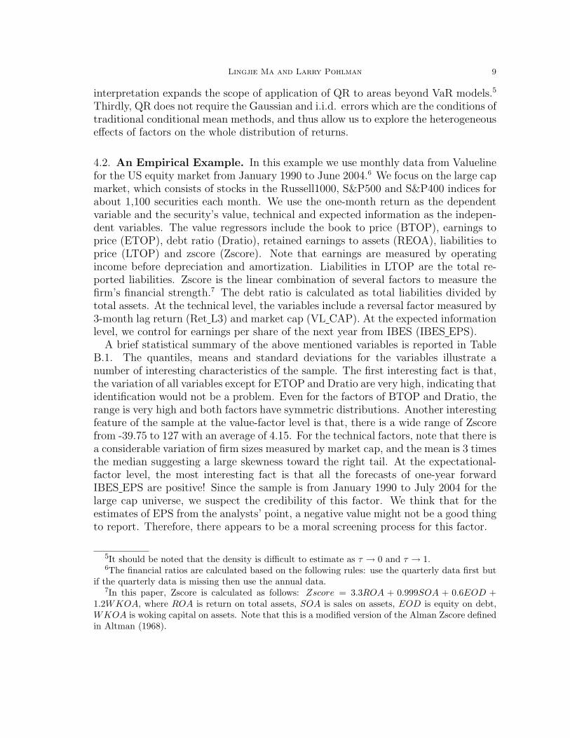
4.2. An Empirical Example. In this example we use monthly data from Valuelinefor the US equity market from January 1990 to June 2004.6 We focus on the large capmarket, which consists of stocks in the Russell1000, S&P500 and S&P400 indices forabout 1,100 securities each month. We use the one-month return as the dependentvariable and the security’s value, technical and expected information as the indepen-dent variables. The value regressors include the book to price (BTOP), earnings toprice (ETOP), debt ratio (Dratio), retained earnings to assets (REOA), liabilities toprice (LTOP) and zscore (Zscore). Note that earnings are measured by operatingincome before depreciation and amortization. Liabilities in LTOP are the total re-ported liabilities. Zscore is the linear combination of several factors to measure thefirm’s financial strength.7 The debt ratio is calculated as total liabilities divided bytotal assets. At the technical level, the variables include a reversal factor measured by3-month lag return (Ret L3) and market cap (VL CAP). At the expected informationlevel, we control for earnings per share of the next year from IBES (IBES EPS).

A brief statistical summary of the above mentioned variables is reported in TableB.1. The quantiles, means and standard deviations for the variables illustrate anumber of interesting characteristics of the sample. The first interesting fact is that,the variation of all variables except for ETOP and Dratio are very high, indicating thatidentification would not be a problem. Even for the factors of BTOP and Dratio, therange is very high and both factors have symmetric distributions. Another interestingfeature of the sample at the value-factor level is that, there is a wide range of Zscorefrom -39.75 to 127 with an average of 4.15. For the technical factors, note that there isa considerable variation of firm sizes measured by market cap, and the mean is 3 timesthe median suggesting a large skewness toward the right tail. At the expectational-factor level, the most interesting fact is that all the forecasts of one-year forwardIBES EPS are positive! Since the sample is from January 1990 to July 2004 for thelarge cap universe, we suspect the credibility of this factor. We think that for theestimates of EPS from the analysts’ point, a negative value might not be a good thingto report. Therefore, there appears to be a moral screening process for this factor.

5It should be noted that the density is difficult to estimate as τ → 0 and τ → 1.6The financial ratios are calculated based on the following rules: use the quarterly data first but

if the quarterly data is missing then use the annual data.7In this paper, Zscore is calculated as follows: Zscore = 3.3ROA + 0.999SOA + 0.6EOD +

1.2WKOA, where ROA is return on total assets, SOA is sales on assets, EOD is equity on debt,WKOA is woking capital on assets. Note that this is a modified version of the Alman Zscore definedin Altman (1968).


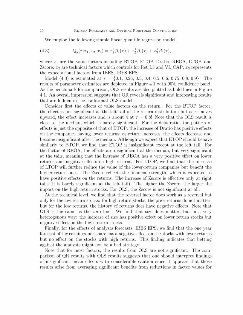
We employ the following simple linear quantile regression model,

Qy(τ |x1, x2, x3) = x>1 β1(τ) + x>2 β2(τ) + x>3 β3(τ),(4.3)

where x1 are the value factors including BTOP, ETOP, Dratio, REOA, LTOP, andZscore; x2 are technical factors which controls for Ret L3 and VL CAP; x3 representsthe expectational factors from IBES, IBES EPS.

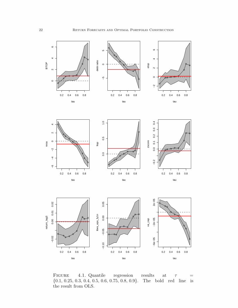
Model (4.3) is estimated at τ = 0.1, 0.25, 0.3, 0.4, 0.5, 0.6, 0.75, 0.8, 0.9. Theresults of parameter estimates are depicted in Figure 4.1 with 90% confidence band.As the benchmark for comparison, OLS results are also plotted as bold lines in Figure4.1. An overall impression suggests that QR reveals significant and interesting resultsthat are hidden in the traditional OLS model.

Consider first the effects of value factors on the return. For the BTOP factor,the effect is not significant at the left tail of the return distribution but as τ movesupward, the effect increases and is about 4 at τ = 0.8! Note that the OLS result isclose to the median, which is barely significant. For the debt ratio, the pattern ofeffects is just the opposite of that of BTOP: the increase of Dratio has positive effectson the companies having lower returns; as return increases, the effects decrease andbecome insignificant after the median. Although we expect that ETOP should behavesimilarly to BTOP, we find that ETOP is insignificant except at the left tail. Forthe factor of REOA, the effects are insignificant at the median, but very significantat the tails, meaning that the increase of REOA has a very positive effect on lowerreturns and negative effects on high returns. For LTOP, we find that the increaseof LTOP will further reduce the value of the lower-return companies but benefit thehigher-return ones. The Zscore reflects the financial strength, which is expected tohave positive effects on the returns. The increase of Zscore is effective only at righttails (it is barely significant at the left tail). The higher the Zscore, the larger theimpact on the high-return stocks. For OLS, the Zscore is not significant at all.

At the technical level, we find that the reversal factor does work as a reversal butonly for the low return stocks: for high return stocks, the prior returns do not matter,but for the low returns, the history of returns does have negative effects. Note thatOLS is the same as the zero line. We find that size does matter, but in a veryheterogenous way: the increase of size has positive effect on lower return stocks butnegative effect on the high return stocks.

Finally, for the effects of analysts forecasts, IBES EPS, we find that the one yearforecast of the earnings-per-share has a negative effect on the stocks with lower returnsbut no effect on the stocks with high returns. This finding indicates that bettingagainst the analysts might not be a bad strategy.

Note that for most factors, the results from OLS are not significant. The com-parison of QR results with OLS results suggests that one should interpret findingsof insignificant mean effects with considerable caution since it appears that thoseresults arise from averaging significant benefits from reductions in factor values for


high return stocks and significant benefits from increase in factor values for low returnstocks.

4.3. Advantages and Challenges. It is clear that there are advantages of quan-tile regression over the traditional ones such as least squares. First of all, instead ofthe point estimate for the conditional mean, we have the whole distribution. Withτ varying in the range of (0, 1) we potentially have different β(τ). Therefore wewould know not only the expected average return, but the whole distribution of theexpected return in the next period given the information known at the current mo-ment. Secondly, as shown earlier, the conditional mean result could be derived fromthe conditional quantile effect. In particular if the distribution of causal effects arenot too skewed, the conditional mean effect would be close to the median. There-fore, for the same sample, quantile regression reveals more information than classicalmethods.

For our return forecasting and final portfolio construction, the main concern ishow the quantile regression method can be used to yield more reasonable forecastsof returns and hence the optimal portfolio. For the classical approach, we have onlyone set of point estimates, and then one forecast for each stock for the asset return.

For example, for the conditional mean approach, we only have E(yi,t+1|xi,t) for eachstock i. But now given multiple sets of forecasted returns, say, for example, at theconventional quantiles,

τ = 0.1, 0.25, 0.5, 0.75, 0.9,

the forecasts of return will be

Qyi(0.1|xi), Qyi

(0.25|xi), Qyi(0.5|xi), Qyi

(0.75|xi), Qyi(0.9|xi).

How can we take advantage of such distribution information to have more accurateforecasts and more value-added portfolio? To the best of our knowledge for quantita-tive analysis of equity models, this is the first study to address and investigate suchan issue. We explore the answers in the next section.

5. return forecast and portfolio construction using distributionalinformation

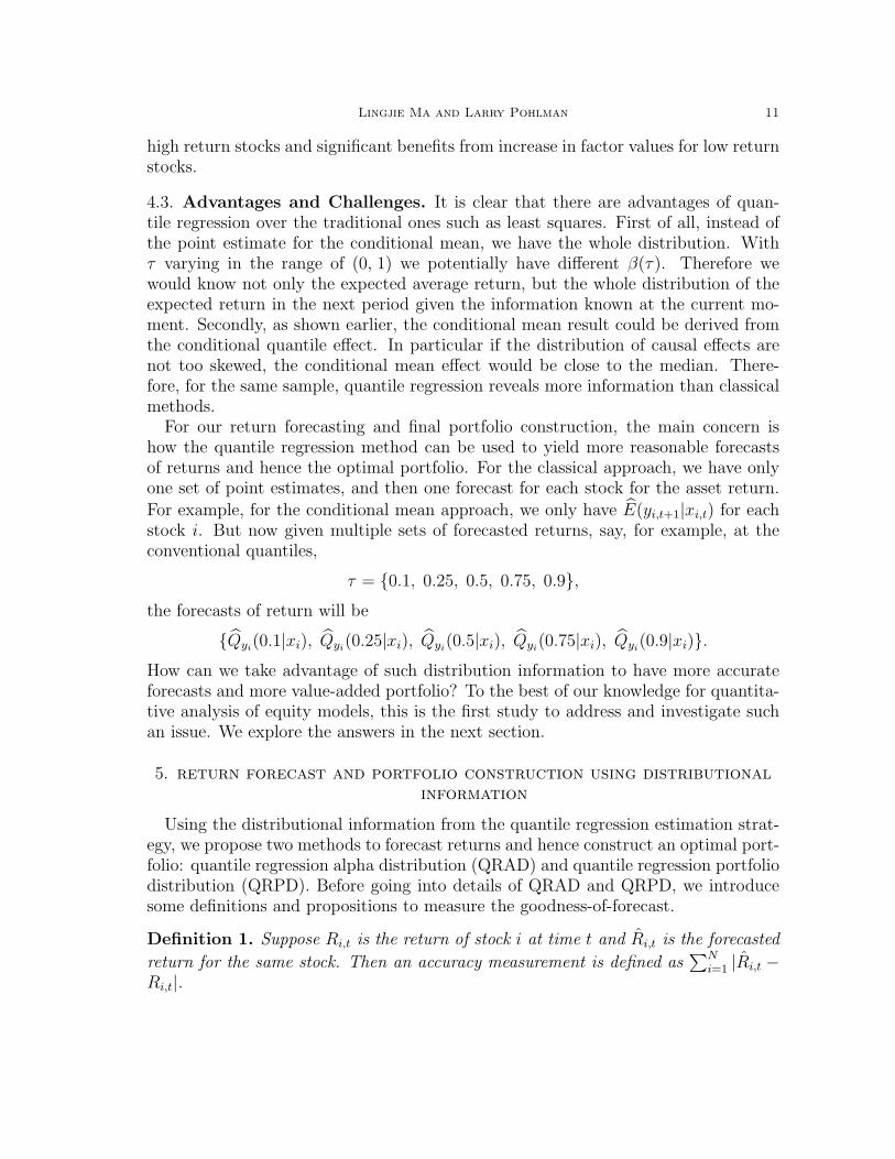
Using the distributional information from the quantile regression estimation strat-egy, we propose two methods to forecast returns and hence construct an optimal port-folio: quantile regression alpha distribution (QRAD) and quantile regression portfoliodistribution (QRPD). Before going into details of QRAD and QRPD, we introducesome definitions and propositions to measure the goodness-of-forecast.

Definition 1. Suppose Ri,t is the return of stock i at time t and Ri,t is the forecasted

return for the same stock. Then an accuracy measurement is defined as∑N

i=1 |Ri,t −Ri,t|.


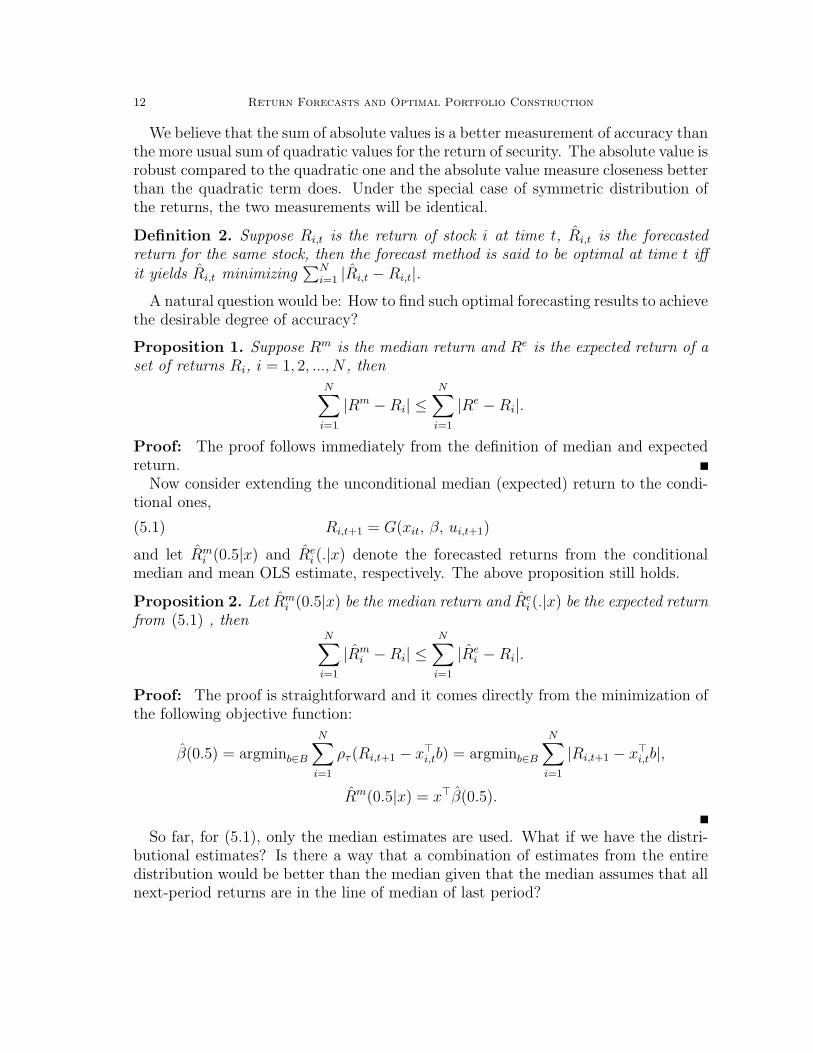
We believe that the sum of absolute values is a better measurement of accuracy thanthe more usual sum of quadratic values for the return of security. The absolute value isrobust compared to the quadratic one and the absolute value measure closeness betterthan the quadratic term does. Under the special case of symmetric distribution ofthe returns, the two measurements will be identical.

Definition 2. Suppose Ri,t is the return of stock i at time t, Ri,t is the forecastedreturn for the same stock, then the forecast method is said to be optimal at time t iffit yields Ri,t minimizing

∑Ni=1 |Ri,t −Ri,t|.

A natural question would be: How to find such optimal forecasting results to achievethe desirable degree of accuracy?

Proposition 1. Suppose Rm is the median return and Re is the expected return of aset of returns Ri, i = 1, 2, ..., N , then

N∑i=1

|Rm −Ri| ≤N∑

i=1

|Re −Ri|.

Proof: The proof follows immediately from the definition of median and expectedreturn.

Now consider extending the unconditional median (expected) return to the condi-tional ones,

Ri,t+1 = G(xit, β, ui,t+1)(5.1)

and let Rmi (0.5|x) and Re

i (.|x) denote the forecasted returns from the conditionalmedian and mean OLS estimate, respectively. The above proposition still holds.

Proposition 2. Let Rmi (0.5|x) be the median return and Re

i (.|x) be the expected returnfrom (5.1) , then

N∑i=1

|Rmi −Ri| ≤

N∑i=1

|Rei −Ri|.

Proof: The proof is straightforward and it comes directly from the minimization ofthe following objective function:

β(0.5) = argminb∈B

N∑i=1

ρτ (Ri,t+1 − x>i,tb) = argminb∈B

N∑i=1

|Ri,t+1 − x>i,tb|,

Rm(0.5|x) = x>β(0.5).

So far, for (5.1), only the median estimates are used. What if we have the distri-butional estimates? Is there a way that a combination of estimates from the entiredistribution would be better than the median given that the median assumes that allnext-period returns are in the line of median of last period?


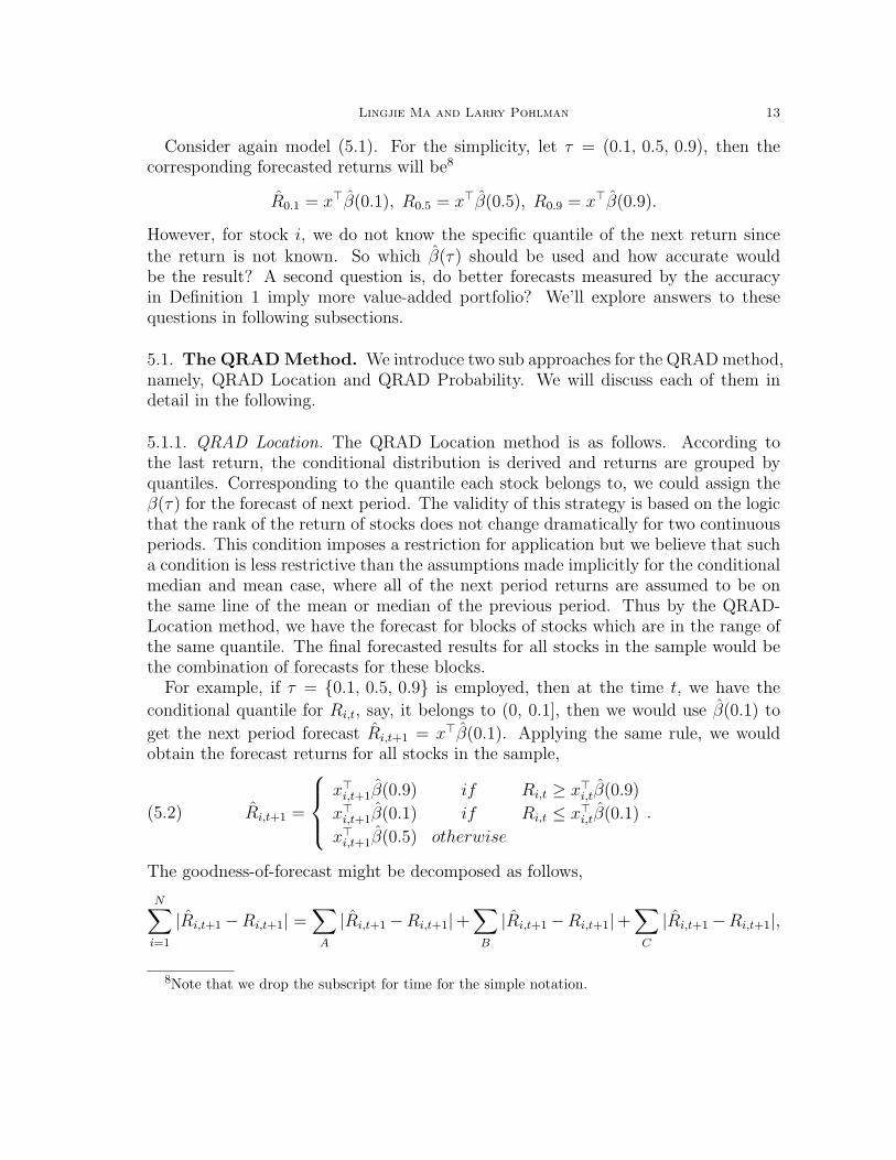
Consider again model (5.1). For the simplicity, let τ = (0.1, 0.5, 0.9), then thecorresponding forecasted returns will be8

R0.1 = x>β(0.1), R0.5 = x>β(0.5), R0.9 = x>β(0.9).

However, for stock i, we do not know the specific quantile of the next return sincethe return is not known. So which β(τ) should be used and how accurate wouldbe the result? A second question is, do better forecasts measured by the accuracyin Definition 1 imply more value-added portfolio? We’ll explore answers to thesequestions in following subsections.

5.1. The QRAD Method. We introduce two sub approaches for the QRAD method,namely, QRAD Location and QRAD Probability. We will discuss each of them indetail in the following.

5.1.1. QRAD Location. The QRAD Location method is as follows. According tothe last return, the conditional distribution is derived and returns are grouped byquantiles. Corresponding to the quantile each stock belongs to, we could assign theβ(τ) for the forecast of next period. The validity of this strategy is based on the logicthat the rank of the return of stocks does not change dramatically for two continuousperiods. This condition imposes a restriction for application but we believe that sucha condition is less restrictive than the assumptions made implicitly for the conditionalmedian and mean case, where all of the next period returns are assumed to be onthe same line of the mean or median of the previous period. Thus by the QRAD-Location method, we have the forecast for blocks of stocks which are in the range ofthe same quantile. The final forecasted results for all stocks in the sample would bethe combination of forecasts for these blocks.

For example, if τ = 0.1, 0.5, 0.9 is employed, then at the time t, we have the

conditional quantile for Ri,t, say, it belongs to (0, 0.1], then we would use β(0.1) to

get the next period forecast Ri,t+1 = x>β(0.1). Applying the same rule, we wouldobtain the forecast returns for all stocks in the sample,

Ri,t+1 =

x>i,t+1β(0.9) if Ri,t ≥ x>i,tβ(0.9)

x>i,t+1β(0.1) if Ri,t ≤ x>i,tβ(0.1)

x>i,t+1β(0.5) otherwise

.(5.2)

The goodness-of-forecast might be decomposed as follows,

N∑i=1

|Ri,t+1−Ri,t+1| =∑

A

|Ri,t+1−Ri,t+1|+∑B

|Ri,t+1−Ri,t+1|+∑

C

|Ri,t+1−Ri,t+1|,

8Note that we drop the subscript for time for the simple notation.


where A, B and C denotes the area of (0, 0.1], (0.1, 0.9) and [0.9, 1), respectively, forthe quantile location of Ri,t (See Figure 5.1). The relative accuracy of the forecastsbased on the QRAD Location method is stated in the following proposition.

Proposition 3. Let Rl(τ |x) be the composite quantile return from the QRAD Loca-

tion method, also Rm(0.5|x) and Re(.|x) be the median and mean return from (5.1),respectively, then

N∑i=1

|Rli,t+1 −Ri,t+1| ≤

N∑i=1

|Rmi,t+1 −Ri,t+1| ≤

N∑i=1

|Rei,t+1 −Ri,t+1|,

where the letter l, m and e denotes location, median and mean, respectively.

Proof: We need the proof only for the first inequality. Let ∆1 ≡ |Rli,t − Ri,t| and

∆1 ≡∑N

i=1 |Rmi,t −Ri,t|. The decomposition by location yields

∆1 =∑

A

|R0.1i,t+1 −Ri,t+1|+

∑B

|Rmi,t+1 −Ri,t+1|+

∑C

|R0.9i,t+1 −Ri,t+1|,

∆2 =∑

A

|Rmi,t+1 −Ri,t+1|+

∑B

|Rmi,t+1 −Ri,t+1|+

∑C

|Rmi,t+1 −Ri,t+1|.

Then, ∆1 ≤ ∆2 is equivalent to∑A

|R0.1i,t+1 −Ri,t+1|+

∑C

|R0.9i,t+1 −Ri,t+1| ≤

∑A

|Rmi,t+1 −Ri,t+1|+

∑C

|Rmi,t+1 −Ri,t+1|.

By the condition that for stocks with Ri,t ∈ A,

Prob.(Ri,t+1 ∈ A) ≥ Prob.(Ri,t+1 ∈ B) and Prob.(Ri,t+1 ∈ A) ≥ Prob.(Ri,t+1 ∈ C),

we have ∑A

|R0.1i,t+1 −Ri,t+1| ≤

∑A

|Rmi,t+1 −Ri,t+1|.

The same inequality holds for C. The final result follows immediately from thecombination.

The results of Proposition 3 can be extended to situations with more than threeareas. However, it should be noted that there is the trade off between the number ofdivisions and the accuracy of forecast.

5.1.2. QRAD Probability. To overcome the disadvantage of the QRAD Location methodwhere forecasts depend heavily on previous conditional location, we propose an alter-native approach, which is to assign probabilities to the forecasts,

Rpi,t+1 = p1R1,i,t+1 + p2R2,i,t+1 + ... + pkRk,i,t+1,

where pk is the probability of the occurence of Rk,i,t+1. For example, for τ =0.1, 0.5, 0.9, we would have that

(p1, p2, p3) = (0.1, 0.8, 0.1),


and,

(R1,i,t+1, R2,i,t+1, R3,i,t+1) = x>i,t(β(0.1), β(0.5), β(0.9)

).

Clearly, the above formulation is the familiar expected value. However, it should benoted that the expected forecasted return is not identical to the forecast of expected

return in general case, that is, ER 6= ER.It can be shown that,

N∑i=1

|Rpi,t+1 −Ri,t+1| ≤

N∑i=1

|Rmi,t+1 −Ri,t+1| ≤

N∑i=1

|Rei,t+1 −Ri,t+1|.

Under mild conditions, both QRAD Location and QRAD Probability yield bettergoodness-of-forecast than the traditional methods. What is the relationship betweenQRAD Location and QRAD Probability? We find that Rp

i,t+1 = ERli,t+1. Note that

from (5.2), under the conditions in Proposition 3 and by the definition of quantileregression, the probability chart (Figure 5.2) follows. In other words, the two methodsare asymptotically the same. Thus we have used more information to construct theforecast and these forecasted results are more accurate than the conditional meanforecast which does not differentiate the factor effects for different level of returns.

5.2. The QRPD Method. The QRPD method differs from the QRAD method inthat we use the distributional information at the optimization stage.

Corresponding to the forecasted returns at each conditional quantile, the optimal

portfolio can be constructed. Let Wτ =(w1,τ , ..., wN,τ

)>be the optimal weights

of the portfolio resulted from using the τth quantile regression forecasted returns.Then with τ ∈ (0, 1), we have an empirical distribution of the portfolio at time t.A natural question is, how to carry out the actual portfolio selection with so many“optimal” choices? Using the same strategy as the QRAD-probability method, thefinal portfolio at time t might be constructed as follows

W = p1Wτ1 + ... + pkWτk,

where pk is the probability of occurence of Wτk. For example, as τ = 0.1, 0.5, 0.9,

we would have three sets of weights, W0.1, W0.5 and W0.9, corresponding to the threesets of forecasting returns. Thus, the weights of the proposed portfolio will be

W = 0.1W0.1 + 0.8W0.5 + 0.1W0.9.

With this new portfolio construction methodology, there are two questions we needto answer. First of all, what is the relationship between QRAD and QRPD? Do theyyield the same portfolio? Second, does the portfolio constructed from the QRPDmethod outperform those from the median or mean forecast? That is, if the perfor-mance is measured by the value added subject to the same constraints and the samebenchmark, does the inequality, W>

q R ≥ W>mR, hold?


To explore the answer to the first question, consider the following standard objectivefunction,

maxW

W>R− λW>ΩW,(5.3)

where Ω is the covariance matrix of R, λ is the risk acceptance parameter. Withthe same value of λ, we derive the sufficient conditions that the methods of QRAD-Probability and QRPD yield the same portfolio. Assume that R1 is independent ofR2 and that Ω1 = Ω2. Furthremore, suppose Rk is the forecasted returns from τk

quantile regression, then by QRAD Probability, we have

R = p1R1 + p2R2.

The first order condition of (5.3) yields

Wqrpd =1

2λΩ−1R

=1

2λ(p21 + p2

2)(p1Ω

−11 R1 + p2Ω

−12 R2)

=1

p21 + p2

2

(p1W1 + p2W2)

= Wqradp.

The assumption of equality of the covariance matrix is too restrictive to be true ingeneral. However, if the objective function is convex, then by Jenson’s inequality, itis expected that the following inequality of portfolio value holds: VQRAD−Probability ≥VQRPD.

Regarding the second question, our answer is that it is not necessary althoughthe probability is positive. This is simply because of the constraints imposed at theoptimization stage. Since any forecast would not completely dominate another in thesense of point by point but rather in a law of large number sense, then the constraintsmight end up restricting the feasible set to an area where the better forecasts arenot active. However, from the statistical perspective, it is expected that in general,the better forecasts would give us more chances to construct a better portfolio. Themathematical version of this argument is provided in the appendix.

6. conclusion

The quantitative analysis for the equity return forecasting and hence portfolioconstruction is becoming more and more popular in both the academic and industrialworld. The statistical methodology such as estimation of expected returns plays acentral role in the quantitative analysis. However, most of the analytical approachesare based on the conditional mean method, which ignores the heterogeneity of theeffects of factors on returns.


In this paper, we emphasize the heterogeneity issue from the response side andintroduce quantile regression as a natural statistical tool to tackle such an issue. Wepresent a general interpretation of the quantile regression results for equity modelsby expanding the interpretation to not only conditional risk but also the conditionalreturn as well. Regarding quantile regression as a general alternative approach to theclassical conditional mean method, we then focus on the return forecast and portfolioconstruction taking advantage of the distribution information from quantile regres-sion. The main challenge is how to utilize the distribution information to constructmore accurate forecast and better-performing portfolios given that the quantile offuture return is unkown. To accomplish such tasks, we propose two methods, QRADand QRPD, where the former utilizes the distributional information at the forecastingstage while the latter at the portfolio construction stage.

By using the goodness-of-forecast measurement, we show that results from bothQRAD and QRPD outperform the results from traditional methods. Regarding thefuture research, we plan to employ these proposed methods to carry out an empiricalstudy for US equity market.


References

[1] Amemiya, T.: “Two Stage Least Absolute Deviations Estimators”, Econometrica, 50, 689–711,1982.

[2] Barnes, M and Hughes, A.: “A Quantile Regression Analysis of the Cross Section of StockMarket Returns”, forthcoming, Journal of Finance.

[3] Bassett, G and Chen, H.: “Portfolio Style: Return-Based Attribution Using Quantile Regres-sion”, Empirical Economics, Springer-Verlag, pp. 1405–1441, 2001.

[4] Blundell, R and Powell, J.: “Endogeneity in Nonparametric and Semiparametric RegressionModels”, in Advances in Economics and Econonometrics: Theory and Applications, EighthWorld Congress, Cambridge University Press, 2003.

[5] Chen, M and Chen, J.: “Application of Quantile Regression to estimation of value at Risk”,working paper, 2003.

[6] Chernozhukov, V. and Hansen, C.: “An IV Model of Quantile Treatment Effects”, forthcoming,Econometrica.

[7] Chesher, A.: “Identification in Nonseparable Models”, Econometrica, vol. 71, No. 5, pp. 1405–1441, 2003.

[8] Diebold, F.: “Forecast Combination and Encompassing: Reconciling Two Divergent Litera-tures”, International Journal of Forecasting, vol. 5, pp. 589–592, 1989.

[9] Engle, R. and Manganelli, S.: “CAViaR: Conditional Autoregressive Value at Risk by RegressionQuantiles”, Journal of Business and Economic Statistics, 2004.

[10] Fama, E. and French, K.: “The Cross-section of Expected Stock Returns”, Journal of Fi-nance,vol. 47, pp. 427-465, 1992.

[11] Hendry, D. and Richard, J.: “On the Formulation of Empirical Models in Dynamic Economet-rics”, Journal of Econometrics, vol. 20, pp. 3–33, 1982.

[12] Ihaka, R. and Gentleman, R.: “R, A Language for Data Analysis and Graphics”, Journal ofGraphical and Computational Statistics, 5, 299-314, 1996.

[13] Jureckova, J. and Prochazka, B.: “Regression Quantiles and Trimmed Least Squares in Non-linear Regression Model”, Journal of Nonparametric Statistics, 3, 201-222, 1994.

[14] Koenker, R.: “Quantiles Regression”, Cambridge University Press, forthcoming, 2005.[15] Koenker, R. and Bassett, G.: “Regression Quantiles”, Econometrica, 46, 33–50, 1978.[16] Koenker, R. and Park, B.: “An Interior Point Algorithm for Nonlinear Quantile Regression”,

Journal of Econometrics, 71, 265-285, 1996.[17] Koenker, R. and Zhao, Q.:“L-estimation for the Linear Heteroscedastic Models”, Journal of

Nonparametric Statistics, 3, 223-235, 1994.[18] Koenker, R. “Quantreg: A Quantile Regression Package for R,” http://cran.r-project.org,

1998.[19] Kordas, G.: “Smoothed Binary Quantile Regression”, Journal of Applied Econometrics, 2004.[20] Kordas, G.: “Credit Scoring Using Binary Quantile Regression”, in Statistical Data Analysis

Based on the L1-Norm and Related Methods, Yalolah Dodge (editor), 2002, Birkhauser.[21] Konno, H. and Yamazaki, H.:“Mean-Absolute Deviation Portfolio Optimization Model and Its

Applications to tokyo Stock Market”, Management Science, Vol. 37, No. 5, 519-531, 1991.[22] Lakonishok, J., Shleifer, A. and Vishny, R.: “The Impact of Institutional Trading on Stock-

prices”, Journal of Financial Economics, vol. 32, August, pp. 2343, 1992.[23] Ma, L. and Koenker, R.: “Quantile Regression Methods for Recursive Structural Equation

Models”, working paper, 2004.[24] Mizon, G and Richard, J.: “The Encompassing Principle and its Application to Testing Non-

nested Hypothesis”, Econometrica, vol. 54, pp. 657–678, 1986.


[25] Oberhofer, W.: “The Consistency of Nonlinear Regression Minimizing The L1 Norm”, TheAnnals of Statistics, 10, 316-19, 1982.

[26] Powell, J.: “The Asymptotic Normality of Two Stage Least Absolute Deviations Estimators”,Econometrica, 51, 1569–1575, 1983.

[27] Sharpe, W.: “Capital Asset Prices: A Theory of Market Equilibrium under Conditions of Risk”,Journal of Finance, vol. 19 (3), pp. 425-442, 1964.

[28] Zhao, Q.: “Asymptotically Efficient Median Regression in the Presence of Heterocesdasticityof Unknown Form”, Econometric Theory, 17, 765-84, 2001.


Appendix A. Proposition 4

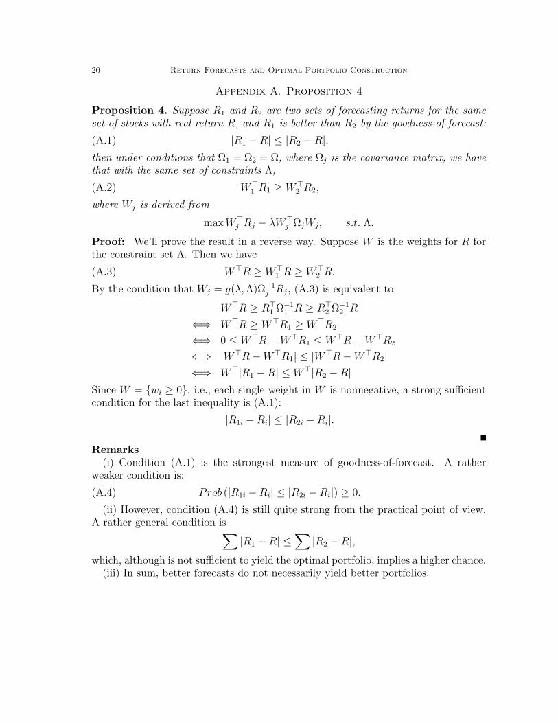
Proposition 4. Suppose R1 and R2 are two sets of forecasting returns for the sameset of stocks with real return R, and R1 is better than R2 by the goodness-of-forecast:

|R1 −R| ≤ |R2 −R|.(A.1)

then under conditions that Ω1 = Ω2 = Ω, where Ωj is the covariance matrix, we havethat with the same set of constraints Λ,

W>1 R1 ≥ W>

2 R2,(A.2)

where Wj is derived from

max W>j Rj − λW>

j ΩjWj, s.t. Λ.

Proof: We’ll prove the result in a reverse way. Suppose W is the weights for R forthe constraint set Λ. Then we have

W>R ≥ W>1 R ≥ W>

2 R.(A.3)

By the condition that Wj = g(λ, Λ)Ω−1j Rj, (A.3) is equivalent to

W>R ≥ R>1 Ω−1

1 R ≥ R>2 Ω−1

2 R

⇐⇒ W>R ≥ W>R1 ≥ W>R2

⇐⇒ 0 ≤ W>R−W>R1 ≤ W>R−W>R2

⇐⇒ |W>R−W>R1| ≤ |W>R−W>R2|⇐⇒ W>|R1 −R| ≤ W>|R2 −R|

Since W = wi ≥ 0, i.e., each single weight in W is nonnegative, a strong sufficientcondition for the last inequality is (A.1):

|R1i −Ri| ≤ |R2i −Ri|.

Remarks(i) Condition (A.1) is the strongest measure of goodness-of-forecast. A rather

weaker condition is:

Prob (|R1i −Ri| ≤ |R2i −Ri|) ≥ 0.(A.4)

(ii) However, condition (A.4) is still quite strong from the practical point of view.A rather general condition is∑

|R1 −R| ≤∑

|R2 −R|,

which, although is not sufficient to yield the optimal portfolio, implies a higher chance.(iii) In sum, better forecasts do not necessarily yield better portfolios.


Appendix B. Table for Summary of Factor Statistics

Tablepanasummary .5.5.5


0.2 0.4 0.6 0.8

02

46

tau

BT

OP

o

oo o o o

o

oo

0.2 0.4 0.6 0.8

−5

05

tau

de

bt ra

tio

o

o o

oo

o o o

o

0.2 0.4 0.6 0.8

−2

02

46

tau

eto

p

o

o o o o o

o

oo

0.2 0.4 0.6 0.8

−6

−4

−2

02

4

tau

reo

a

o

oo

oo

o

o

o

o

0.2 0.4 0.6 0.8

0.0

0.5

1.0

tau

ltop

o

o oo

oo o o

o

0.2 0.4 0.6 0.8

−0

.20

.00

.10

.20

.30

.4

tau

zsco

re

o

o o o o o

o

o o

0.2 0.4 0.6 0.8

−0

.02

0.0

00

.01

0.0

2

tau

retu

rn_

lag

3

oo

o oo

o

oo o

0.2 0.4 0.6 0.8

−0

.10

−0

.05

0.0

00

.05

tau

ibe

s_e

ps_

fy1

n

o o o

o o o

oo o

0.2 0.4 0.6 0.8

−6

e−

05

−2

e−

05

2e

−0

5

tau

va_

cap

oo o

oo o

oo

o

Figure 4.1. Quantile regression results at τ =0.1, 0.25, 0.3, 0.4, 0.5, 0.6, 0.75, 0.8, 0.9. The bold red line isthe result from OLS.


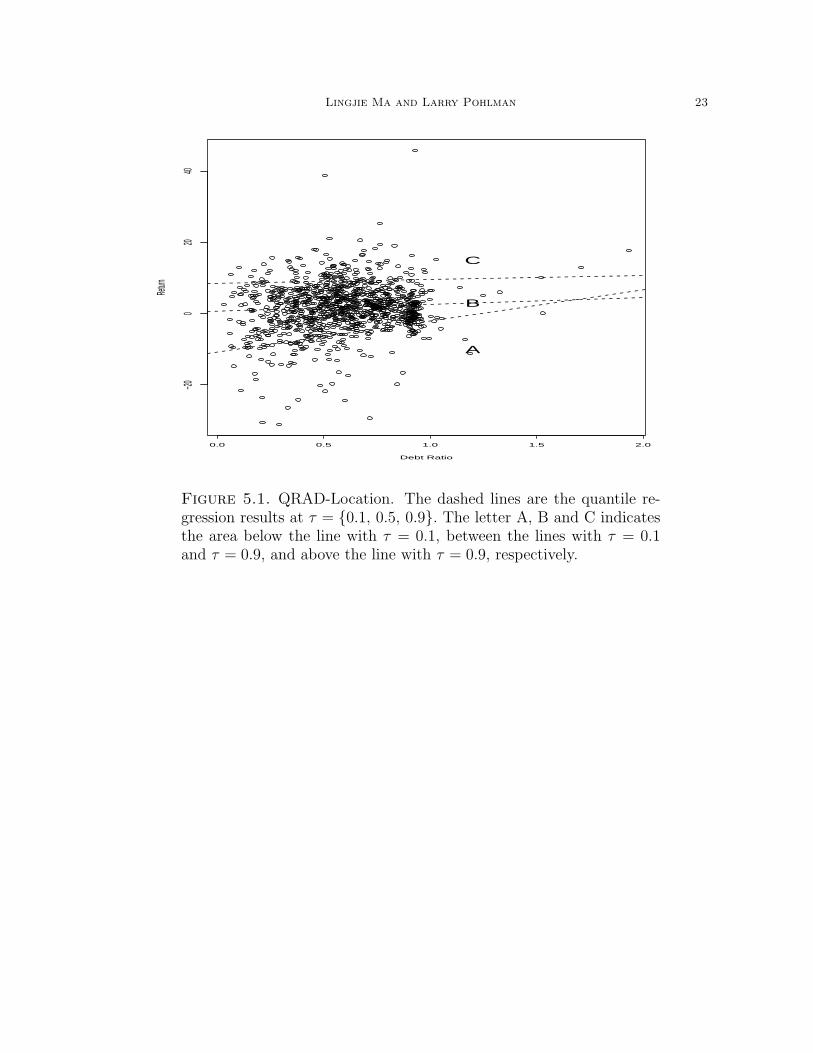
0.0 0.5 1.0 1.5 2.0

−200

2040

Debt Ratio

Return

A

B

C

Figure 5.1. QRAD-Location. The dashed lines are the quantile re-gression results at τ = 0.1, 0.5, 0.9. The letter A, B and C indicatesthe area below the line with τ = 0.1, between the lines with τ = 0.1and τ = 0.9, and above the line with τ = 0.9, respectively.


P=0.1

P=0.8

P=0.1

b(0.1)

b(0.5)

b(0.9)

R_it

Figure 5.2. Probability of QRAD-Location.

RETURN FORECASTS AND OPTIMAL PORTFOLIO CONSTRUCTION

Documents

Transcript of RETURN FORECASTS AND OPTIMAL PORTFOLIO CONSTRUCTION