Geometric GAN

Jae Hyun Lim1, Jong Chul Ye2,31 ETRI, South Korea

jaehyun.lim@etri.re.kr2 Dept. of Bio and Brain engineering, KAIST, South Korea3 Dept. of Mathematical Sciences, KAIST, South Korea

jong.ye@kaist.ac.kr

Abstract

Generative Adversarial Nets (GANs) represent an important milestone for effec-tive generative models, which has inspired numerous variants seemingly differentfrom each other. One of the main contributions of this paper is to reveal a unifiedgeometric structure in GAN and its variants. Specifically, we show that the ad-versarial generative model training can be decomposed into three geometric steps:separating hyperplane search, discriminator parameter update away from the sep-arating hyperplane, and the generator update along the normal vector direction ofthe separating hyperplane. This geometric intuition reveals the limitations of theexisting approaches and leads us to propose a new formulation called geometricGAN using SVM separating hyperplane that maximizes the margin. Our theo-retical analysis shows that the geometric GAN converges to a Nash equilibriumbetween the discriminator and generator. In addition, extensive numerical resultsshow that the superior performance of geometric GAN.

1 Introduction

Recently, inspired by the success of the deep discriminative models, Goodfellow et al [1] proposeda novel generative model training method called generative adversarial nets (GAN). GAN is formu-lated as a minimax game between a generative network (generator) that maps a random vector intothe data space and a discriminative network (discriminator) trying to distinguish the generated sam-ples from real samples. Unlike the classical generative models such as Variational Auto-Encoders(VAEs) [2], the minimax formation of GAN can transfer the success of deep discriminative modelsto generative models, resulting in significant improvement in generative model performance [1].

Specifically, the original form of the GAN solves the following minmax game:

minG

maxD

LGAN (D,G) (1)

where

LGAN (D,G) := Ex∼PS [logD(x)] + Ez∼PZ [log(1−D(G(z))] , (2)

where PS is the sample distribution; D(x) is the discriminator that takes x ∈ X as input and outputsa scalar between [0, 1]; G(z) is the generator that maps a sample z drawn from a distribution PZto the input space X . The meaning of (1) is that the generator tries to fool out the discriminatorwhile the discriminator wants to maximize the differentiation power between the true and generatedsamples. The authors further showed that the GAN training is indeed to approximate the minimiza-tion of the symmetric Jensen-Shannon divergence [1]. This idea has been generalized by the authorsin [3] for all f -divergences. Moreover, Maximum Mean Discrepancy objective (MMD) for GANtraining was also proposed in [4, 5].

It is well-known that the training GAN is difficult. In particular, the authors in [6] have iden-tified the following sources of the difficulties: 1) when the discriminator becomes accurate, the

arX

iv:1

705.

0289

4v2

[st

at.M

L]

9 M

ay 2

017

gradient for generator vanishes, 2) a popular fixation using a generator gradient updating withEz∼PZ [− logD(G(z))] is unstable because of the singularity at the denominator when the dis-criminator is accurate. The main motivation of Wasserstein GAN (W-GAN) [7] was, therefore, tointroduce the weight clipping to address the above-described limitations. In fact, Wasserstein GANis a special instance of minimizing the integral probability metric (IPM) [8], and Mroueh et al [9]recently generalized the W-GAN for wider function classes and proposed the mean feature matchingand/or covariance feature matching GAN (McGAN) using the IPM minimization framework [9].

Inspired by McGAN, here we propose a novel geometric generalization called geometric GAN.Specifically, geometric GAN is inspired by our novel observation that McGAN is composed ofthree geometric operations in feature space:

• Separating hyperplane search: finding the separating hyperplane for a linear classifier[10, 11, 12]

• Discriminator update away from the hyperplane: discriminator parameter update awayfrom the separating hyperplane using stochastic gradient direction (SGD).

• Generator update toward the hyperplane: generator parameter update along the normalvector direction of the separating hyperplane using stochastic gradient direction (SGD).

This geometric interpretation proves to be very general, so it can be applied to most of the existingGAN and its variants. Indeed, the main differences between the algorithms come from the construc-tion of the separating hyperplanes for a linear classifier on feature space and the geometric scalingfactors for the feature vectors. Based on this observation, we provide new geometric interpretationsof GAN [1], f -GAN [3], EB-GAN [13], and W-GAN [7] in terms of separating hyperplanes andgeometric scaling factors, and discuss their limitations. Furthermore, we propose a novel geomet-ric GAN using the support vector machine (SVM) separating hyperplane that has maximal marginbetween two classes of separable data [14, 11]. Our numerical experiments clearly showed that theproposed geometric GAN outperforms the existing GANs in all data set.

2 Related Approaches

In order to introduce the geometric interpretation of GAN and its variants, we begin with the reviewof the mean feature matching GAN (McGAN) [9].

2.1 Mean feature matching GAN

Let F be a set of bounded real valued functions on the sample space X . Suppose that P and Q aretwo probability distributions on X . Then, the integral probability metric (IPM) between P and Qon the function space F is defined as follows [8, 15, 16]:

dF (P,Q) = supf∈F

∣∣∣∣∫ fdP −∫fdQ

∣∣∣∣= sup

f∈F|Ex∼P [f(x)]− Ex∼Q[f(x)]| (3)

where Ex∼P [·] denotes the expectation with respect to the probability distribution P (x). We caneasily show that dF is non-negative, symmetric and satisfies the triangle inequality. So dF can beused as a distance measure in the probability space. For example, when F is defined as a collectionof functions with a finite Lipschitz constant, the IPM is the Wasserstein distance or the earth mover’sdistance [15, 16] that forms the basis of the Wasserstein GAN [7].

In McGAN, the generator network gθ : Z → X that maps a random input z ∈ Z to a target x ∈ Xis shown as a block in Fig. 1(a), and the function space F under study is defined as follows [9]:

Fw,ζ = {f(x) = 〈w,Φζ(x)〉 | w ∈ Ξ, ‖w‖2 ≤ 1}where Φζ : X → Ξ is a bounded map from X to a (often higher-dimensional) feature space Ξ. Notethat Fw,ζ is a symmetric function spaces because if f ∈ Fw,ζ , then −f ∈ Fw,ζ . Then, the IPMbetween Px and Pg is given by

dF (Px, Pg) = max‖w‖2≤1

〈w,Ex∼PxΦζ(x)− Egθ∼PgΦζ(gθ)〉

2

Figure 1: Structure of the mean feature matching GAN and its extension to geometric GAN.

under the constraints that Φζ is bounded and ‖w‖2 ≤ 1.

Now, given a finite sequence of mini-batch training data set S = {(z1, x1), · · · , (zn, xn)}, an em-pirical estimate of the minmax game that minimizes the dF (Px, Pg) is given by [9]:

minθ

max‖w‖2≤1,ζ

L(w, ζ, θ) (4)

(5)

where

L(w, ζ, θ) :=

⟨w,

1

n

n∑i=1

Φζ(xi)−1

n

n∑i=1

Φζ(gθ(zi))

⟩

Then, the discriminator update can be done using a stochastic gradient descent (SGD) [9]:

(w, ζ) ← (w, ζ) + η(∇wL(w, ζ, θ),∇ζL(w, ζ, θ)

)(6)

where η is a learning rate. The authors in [9] also used the projection onto the unit lp ball andweight clipping for w and ζ updates, respectively, to meet the constraints. Using the updated w, thegenerator update is then given by [9]:

θ ← θ + η

n∑i=1

〈w,∇θΦ(gθ(zi))〉 /n . (7)

2.2 Geometric interpretation of the mean feature matching GAN

The primal form of the w update in (6) is geometrically less informative, so here we use the Cauchy-Swartz inequality to obtain a closed-form update for w:

w∗ = cn∑i=1

(Φζ(xi)− Φζ(gθ(zi))) /n (8)

where the constant c is given by c = ‖∑ni=1 (Φζ(xi)− Φζ(gθ(zi))) /n‖

12 . Given w∗, the corre-

sponding discriminator and generator updates are represented by

ζ ← ζ + η

n∑i=1

〈w∗,∇ζΦζ(xi) −∇ζΦζ(gθ(zi))〉/n (9)

θ ← θ + η

n∑i=1

〈w∗,∇θΦζ(gθ(zi))〉 /n (10)

Note that the update equations (8) to (10) are equivalent to the dual form of the McGAN [9], wherethe authors derived the following minmax problem by using (8):

minθ

maxζ

1

2

∥∥∥∥∥n∑i=1

Φζ(xi)−n∑i=1

Φζ(gθ(zi))

∥∥∥∥∥2

. (11)

However, we notice that the explicit representation by Eqs. (8) to (10) gives clearer geometricintuition that plays the key role in designing a geometric GAN, ass will become clear soon.

3

More specifically, in designing a linear classifier for two class classification problems, (8) is knownas the normal vector for the separating hyperplane for the mean difference (MD) classifier [10, 11,12]. As shown in Fig. 2, once the separating hyperplane is defined, the SGD udpate (9) is to updatethe discriminator parameters such that the true and fake samples are maximally separately awayfrom the separating hyperplane parallel to the normal vector. On the other hand, the SGD udpateusing (10) is to update the generator parameters to make the fake samples approach the separatinghyperplane along the normal vector direction (see Fig. 2).

Figure 2: Geometry of the mean feature matching GAN.

Recall that a linear classifier is defined via the normal vector to the separating hyperplane and anoffset [14]. Thus, comparing the direction between two classifiers means comparing their normalvector directions. As shown in Appendix, aside from the geometric scaling factors, the existing GANand its variants mainly differ in their definition of the normal vector for the separating hyperplane.Based on this observation, in the next section, we discuss an optimal separating hyperplane forgenerative model training that has the maximal margin.

3 Geometric GAN

3.1 Linear classifiers in high-dimension low-sample size

In adversarial training in feature space, a discriminator is interested in discriminating true samples{Φζ(xi)}ni=1 and the fake samples {Φζ(gθ(zi))}ni=1. In practice, the minibatch size n is muchsmaller than the dimension of the feature space d, and this type of classification problem is oftencalled the high-dimension low-sample size (HDLSS) problem [10, 11, 12].

In fact, the mean difference (MD) classifier is one of the popular methods for HDLSS. Specifically,the MD classifier selects the hyperplane that lies half way between the two class means. In particularthe normal vector w for the seperating hyperplane is given by the difference of the class means:

wMD =1

n

n∑i=1

Φζ(xi)−1

n

n∑i=1

Φζ(gθ(zi)) (12)

Note that if the variables are first mean centered then scaled by the standard deviation, then themean difference is equivalent to the naive Bayes classifier [10, 11, 12]. Furthermore, in HDLSS,there always exists a maximal data piling direction (MDP) [12], where mulitple points in each classhave the identical projection on the line spanned by the normal vector.

On the other hand, the Support Vector Machine (SVM) [14] and its many variants is one of the mostwidely used and well studied classification algorithms and its robustness has been also proven forHDLSS setup [10, 11, 12]. Although the aforementioned classification algorithms are motivated

4

by fitting a statistical distribution to the data, SVM is motivated by a geometric heuristic that leadsdirectly to an optimization problem: maximize the margin between two classes of separable data.In addition, soft-margin SVM balances two competing objectives to maximize the margin whilepenalizing points on the wrong side of the margin.

Recently, Carmichael et al [11] investigated the Karush-Kuhn-Tucker conditions to provide rigorousmathematical proof for new insights into the behaviour of soft-margin SVM in the large and smalltuning parameter regimes in HDLSS. They revealed that for small tuning parameter, if the numberof data in two classes are the same (which is the case in our problem), then the SVM directionbecomes exactly the MD direction. In addition, for sufficiently large tuning parameter, the authorsshowed that soft margin SVM is equivalent to hard margin SVM if the data are separable, and thehard-margin SVM has data piling. Due to this generality of the soft-margin SVM, the proposedgeometric GAN is designed based on soft-margin SVM linear classifier.

3.2 Geometric GAN with SVM hyperplane

Note that soft-margin SVM is designed by adding a tunning parameter C and slack variables ξiwhich allows points to be on the wrong side of the margin [14]. In our problem classifying the truesamples versus fake samples, the primal form of soft-margin SVM can be formulated by

minw,b

12‖w‖

2 + C∑i(ξi + ξ′i)

subject to 〈w,Φζ(xi)〉+ b ≥ 1− ξi, i = 1, · · · , n〈w,Φζ(gθ(zi))〉+ b ≤ ξ′i − 1, i = 1, · · · , nξi, ξ

′i ≥ 0, i = 1, · · · , n

Equivalently, the primal form of the soft-margin SVM can be represented using loss + penalty form[17, 14]:

minw,b

Rθ(w, b; ζ) (13)

where

Rθ(w, b; ζ) =1

2Cn‖w‖2 +

1

n

n∑i=1

max (0, 1− 〈w,Φζ(xi)〉 − b)

+1

n

n∑i=1

max (0, 1 + 〈w,Φζ(gθ(zi))〉+ b) (14)

The goal of the SVM optimization (13) is to maximize the margin between the two classes. Thisimplies that the discriminator update can be also easily incorporated with SVM update, becausethe goal of the discriminator update can be also regarded to maximize the margin between the twoclasses. More specifically, our optimization problem is given by

minw,b,ζ

Rθ(w, b; ζ) (15)

for a given generator parameter θ.

Specifically, in SVM, the normal vector for the optimal separating hyperplane wSVM from (13) isgiven by [11, 14]:

wSVM :=

n∑i=1

αiΦζ(xi)−n∑i=1

βiΦζ(gθ(zi)) (16)

where (αi, βi) will be nonzero only for the support vectors, where the set of support vectors nowincludes all data points on the margin boundary as well as those on the wrong side of the marginboundary (see Fig. 3). More specifically, we define the regionM between the margin boudaries asshown in Fig. 3(a):

M = {φ ∈ Ξ | |〈wSVM , φ〉+ b| ≤ 1} . (17)

5

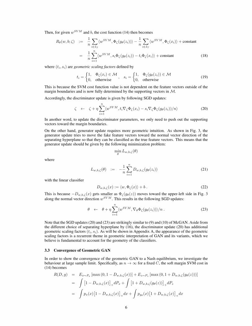
Then, for given wSVM and b, the cost function (14) then becomes

Rθ(w, b; ζ) :=1

n

∑i∈IS

〈wSVM ,Φζ(gθ(zi))〉 −1

n

∑i∈IT

〈wSVM ,Φζ(xi)〉+ constant

=1

n

n∑i=1

〈wSVM , siΦζ(gθ(zi))− tiΦζ(xi)〉+ constant (18)

where (ti, si) are geometric scaling factors defined by

ti =

{1, Φζ(xi) ∈M0, otherwise

, si =

{1, Φζ(gθ(zi)) ∈M0, otherwise

(19)

This is because the SVM cost function value is not dependent on the feature vectors outside of themargin boundaries and is now fully determined by the supporting vectors inM.

Accordingly, the discriminator update is given by following SGD updates:

ζ ← ζ + η

n∑i=1

〈wSVM , ti∇ζΦζ(xi)− si∇ζΦζ(gθ(zi))/n〉 (20)

In another word, to update the discriminator parameters, we only need to push out the supportingvectors toward the margin boundaries.

On the other hand, generator update requires more geometric intuition. As shown in Fig. 3, thegenerator update tries to move the fake feature vectors toward the normal vector direction of theseparating hyperplane so that they can be classified as the true feature vectors. This means that thegenerator update should be given by the following minimization problem:

minθLw,b,ζ(θ)

where

Lw,b,ζ(θ) := − 1

n

n∑i=1

Dw,b,ζ(gθ(zi)) (21)

with the linear classifier

Dw,b,ζ(x) := 〈w,Φζ(x)〉+ b . (22)

This is because −Dw,b,ζ(x) gets smaller as Φζ(gθ(z)) moves toward the upper-left side in Fig. 3along the normal vector direction wSVM . This results in the following SGD updates:

θ ← θ + η

n∑i=1

〈wSVM ,∇θΦζ(gθ(zi))〉/n . (23)

Note that the SGD updates (20) and (23) are strikingly similar to (9) and (10) of McGAN. Aside fromthe different choice of separating hyperplane by (16), the discriminator update (20) has additionalgeometric scaling factors (ti, si). As will be shown in Appendix A, the appearance of the geometricscaling factors is a recurrent theme in geometric interpretation of GAN and its variants, which webelieve is fundamental to account for the geometry of the classifiers.

3.3 Convergence of Geometric GAN

In order to show the convergence of the geometric GAN to a Nash equilibrium, we investigate thebehaviour at large sample limit. Specifically, as n→∞ for a fixed C, the soft margin SVM cost in(14) becomes

R(D, g) = Ex∼Px [max (0, 1−Dw,b,ζ(x))] + Ez∼Pz [max (0, 1 +Dw,b,ζ(gθ(z)))]

=

∫ [1−Dw,b,ζ(x)

]+dPx +

∫ [1 +Dw,b,ζ(gθ(z))

]+dPz

=

∫px(x)

[1−Dw,b,ζ(x)

]+dx+

∫pgθ (x)

[1 +Dw,b,ζ(x)

]+dx

6

Figure 3: Geometric GAN using SVM hyperplane. Discriminator and generator update directionsare shown.

where [x]+ = max{0, x} and Dw,b,ζ(x) is a linear discriminator in (22) parameterized by (w, b, ζ).Here, px(x) and pgθ (x) denote the probability density functions (pdf) for the distribution Px andPz(gθ(z)), respectively. Similarly, the generator cost function in (21) becomes

L(D, g) = −Ez∼Pz [Dw,b,ζ(gθ(z))]

= −∫pgθ (x)Dw,b,ζ(x)dx

Then, the adversarial training between discriminator and generator can be achieved by the followingalternating minimization:

minD

R(D, g) := minw,b,ζ

R(Dw,b,ζ , g) (24)

mingL(D, g) := min

θL(D, gθ) (25)

Suppose that the optimal solution of the aforementioned adversarial training is a pair (D∗, g∗). Then,we can prove the following key convergence result.Theorem 3.1. Suppose that (D∗, g∗) is a minimizer of the alternating minimization of (24) and(25). Then, pg∗(x) = px(x) almost everywhere, and R(D∗, G∗) = 2.

Proof. See Appendix B.

In the following example, we provide a specific example where the discriminator and generator costfunction has close form expressions, which also has intuitive meaning of the minimum value 2 inTheorem 3.1. In particular, we consider an example of learning parallel lines as in the originalWasserstein GAN paper [7].Example 3.1 (Learning parallel lines). Let u ∼ U [0, 1] denote the uniform distribution on the unitinterval. Let Px be the distribution of x = (0, u) ∈ R2, uniform on a straight vertical line passingthrough the origin. Suppose that the generator sample is given by gθ(z) = (θ, z) with θ a singlereal parameter. We can easily see that the SVM separating hyperplane is given by

〈w, x〉+ b = 0

7

where w = (−1, 0), b = θ/2 if θ ≥ 0 and w = (1, 0), b = −θ/2 if θ < 0. Thus, the generator costfunction becomes

L(D, g) = −E [〈w, gθ(z)〉+ b]

= |θ|/2

which achieves its minimum at θ∗ = 0. Then, the corresponding discriminator cost value at n→∞is given by

R(D∗, g∗) = limθ→0

{E [1− 〈w, x〉 − b]+ + E [1 + 〈w, gθ(z)〉+ b]+

}= lim

θ→02 [1− |θ|/2]+

= 2

which coincides the results by Theorem 3.1.

In this example, R(D∗, g∗) = 2 because all the true and fake samples lies on the separating hyper-plane. This informs that at the Nash equilibrium of this problem, all the true samples and the fakesamples are not separable, which is the desired property of GAN training. However, Theorem 3.1is only a necessary condition to make the true and fakes sample non-separable. The proof for thesufficiency condition would be very interesting, which is beyond the scope of current paper.

4 Experimental Results

4.1 Mixture of Gaussians

In order to evaluate the proposed geometric GAN, we perform comparative studies with three rep-resentative types of GANs; 1) Jenson-Shannon (GAN) [1], 2) mean difference in l∞ (WassersteinGAN) [7], and 3) mean difference in l2 [9]. Here, the behavior of the maximum margin separat-ing hyperplane of the geometric GAN is empirically analyzed against those of the aforementionedapproaches.

In addition, to evaluate the dependency of each variants on Lipschitz continuity constraints, theLipschitz constraints suggested in [7, 18] was also applied to each adversarial training approach.More specifically, the parameters (w, b) of the final linear layer in discriminator is determined torepresent the aforementioned hyperplane properties, whereas the Lipschitz constraints are appliedfor other network parameters, such as ζ in Φζ(x) and θ in gθ(z). In this paper, we only considerLipschitz density constraints in [18], so we follow to use weight decay on generators gθ(x) andfeature space mapping φζ(x) in discriminators.

We test the four hyperplane searching approaches for discriminators, as well as their complementarygenerator losses, on two dimensional synthetic data. The synthetic data consists of 100K data pointsgenerated from a mixture of 25 Gaussians, akin to the data that have been used for describing modecollapsing behaviors of GANs [19, 20, 21]. Specifically, the means of the Gaussians are evenlyspaced as a 5 by 5 grid along x and y axis from -21 to 21. The standard deviation of each normaldistribution is 0.316 (so that the variance would be 0.1). The sampled data from the true distributioncan be seen in Figure 4 and 5.

For discriminator and generator, a multi-layered fully-connected neural network architecture is used,as described below. RMSprop [22] is used to train these networks, except vanilla GAN (without anyLipschitz constraints). For vanilla GAN, Adam [23] with momentum β1 = 0.5 is used. Baselearning rate is set to 0.001. When weight clipping is applied, parameters in feature mapping φζ(x)is clipped within the range of [−0.01, 0.01]. When weight projection on unit l2 norm is applied, thefollowing rule, p = min{1, 1/‖p‖2}×p described in [9] is used to update any parameter p for everyiteration. For weight decay, weight decaying parameter is set to 0.001. Batch size is set to 500 forall experiment. For the number of discriminator update Kd and the one of generator update Kg , weset them as 1, i.e. (Kd = 1,Kg = 1).

• Discriminator: FC(2, 128)-ReLU-FC(128, 128)-ReLU-FC(128, 128)-ReLU-FC(128, 1)

• Generator: FC(4, 128)-BN-ReLU-FC(128, 128)-BN-ReLU-FC(128, 128)-BN-ReLU-FC(128, 2)

8

(a) True data (b) GAN [1] (c) Proposed (d) WGAN [7] (e) meanGAN +wproj on φζ [9]

Figure 4: Generated samples of GAN variants for the mixture of 25 Gaussians, and the ones fromthe true data distribution.

(a) True data (b) GAN + wdecayon Φζ and gθ

(c) Proposed +wdecay on Φζ andgθ

(d) WGAN + wde-cay on Φζ and gθ

(e) meanGAN +wdecay on Φζ andgθ

Figure 5: Generated samples of GAN variants under trained with Lipschitz density constraints sug-gested in [18] for the mixture of 25 Gaussians, and the sample from the true data distribution. Duringtraining, weight decay was applied on ζ in Φζ(x) and θ in gθ(z) in addition to their own hyperplaneconstraints.

The results of the experiment with the mixture of 25 Gaussians are illustrated in Figure 4 and 5.Amongst all GAN variants in this experiment, geometric GAN demonstrated the least mode col-lapsing behavior independently with Lipschitz continuity regularization constraints.

As shown in Fig. 5, under the same Lipschitz density constraints, linear hyperplane approachesdemonstrated less mode collapsing behaviors by virtue of consistent gradients unlike nonlinear sep-arating hyperplane of original GAN. However, mean difference-driven hyperplanes in WassersteinGAN or McGAN led generators to the mean of arbitrary number of modes in true distributions sincethe characteristics of mean difference. One the other hand, geometric GAN generally showed robustand consistent convergence behavior towards true distributions.

4.2 Image Datasets

In order to analyze the proposed method on large-scale dataset, the geometric GAN is empiricallyanalyzed on well-studied datasets in the context of adversarial training; MNIST, CelebA, and LSUNdatasets. Since consistent quantitative measures are still under debate, we only perform qualitativecomparisons of generated samples from the learned generators of the propsed method against theresults of previous literatures. In favor of fair comparisons with other adversarial training meth-ods, we adopt the settings from the previous literatures except the hyperparameters of stochasticoptimizations and the tuning parameter of the proposed method.

The DCGAN neural network architectures [24] was used, including batch normalization for gener-ator. Note that the currently known adversarial training methods that demonstrated stable learningwithout batch normalization [7, 9, 18] have resorted to Lipschitz constraints; therefore, it can alsobe applied to other adversarial training criterions, including geometric GAN, in order to train batchnormalization-free generators.

Each pixel value in input image was rescaled to [−1, 1] for all dataset, including MNIST dataset.During all training, mini-batch size was set to 64. For stochastic gradient update during training,RMSprop was used [22]. The number of generator’s updates per each discriminator’s update is setto 10 (Kd = 1,Kg = 10). Learning rate is set to 0.0002 for both discriminators and generators, anda tuning parameter C for discriminator is set to 1.

Specifically for MNIST dataset, input images were resized to 64 by 64 pixels in order to use thesame DCGAN network architecture, and the number of epochs for training was set to 20. ForCelebA dataset, input images were resized to 96 by 96 pixels and center-cropped with 64 by 64pixels, and the number of epochs for training is set to 50. For LSUN dataset, only bedroom dataset

9

is used, and an input image is resized to 64 by 64 pixels. The number of epochs for training is set to2 for LSUN dataset.

The results in Figure 6, 7, and 8 clearly show that the geometric GAN generates very realisticimages without mode collapsing or divergent behaviours.

Figure 6: Generated samples of Geometric GAN trained for MNIST dataset.

5 Conclusion

This paper proposed a novel geometric GAN using SVM separating hyperplane, based on geometricintuitions revealed from previous adversarial training approaches. The geometric GAN was basedon SVM separating hyperplanes that has the maximal margins between the two classes. Comparedto the most of the existing approaches that are based on statistical design criterion, the geometricGAN is derived based on geometric intuition similar to the derivation of SVM. Extensive numeri-cal experiments showed that the proposed method has demonstrated less mode collapsing and morestable training behavior. Moreover, our theoretical results showed that the proposed algorithm con-verges to the Nash equilibrium between the discriminator and generator, which has also geometricmeaning.

Acknowledgement

This work is supported by Korea Science and Engineering Foundation, Grant numberNRF2016R1A2B3008104. The first author would like to thank Yunhun Jang for helpful discus-sions.

References[1] I. Goodfellow, J. Pouget-Abadie, M. Mirza, B. Xu, D. Warde-Farley, S. Ozair, A. Courville,

and Y. Bengio, “Generative adversarial nets,” in Advances in Neural Information ProcessingSystems, 2014, pp. 2672–2680.

10

Figure 7: Generated samples of Geometric GAN trained for CelebA dataset.

Figure 8: Generated samples of Geometric GAN trained for LSUN dataset.

11

[2] D. P. Kingma and M. Welling, “Auto-encoding variational bayes,” arXiv preprintarXiv:1312.6114, 2013.

[3] S. Nowozin, B. Cseke, and R. Tomioka, “f-GAN: Training generative neural samplers usingvariational divergence minimization,” in Advances in Neural Information Processing Systems,2016, pp. 271–279.

[4] Y. Li, K. Swersky, and R. Zemel, “Generative moment matching networks,” in Proceedings ofThe 32nd International Conference on Machine Learning, 2015, pp. 1718–1727.

[5] G. Dziugaite, D. Roy, and Z. Ghahramani, “Training generative neural networks via maximummean discrepancy optimization,” in Uncertainty in Artificial Intelligence-Proceedings of the31st Conference, UAI 2015, 2015, pp. 258–267.

[6] M. Arjovsky and L. Bottou, “Towards principled methods for training generative adversarialnetworks,” in NIPS 2016 Workshop on Adversarial Training. In review for ICLR, vol. 2016,2017.

[7] M. Arjovsky, S. Chintala, and L. Bottou, “Wasserstein GAN,” arXiv preprintarXiv:1701.07875, 2017.

[8] A. Muller, “Integral probability metrics and their generating classes of functions,” Advances inApplied Probability, vol. 29, no. 02, pp. 429–443, 1997.

[9] Y. Mroueh, T. Sercu, and V. Goel, “McGan: Mean and covariance feature matching GAN,”arXiv preprint arXiv:1702.08398, 2017.

[10] J. S. Marron, M. J. Todd, and J. Ahn, “Distance-weighted discrimination,” Journal of theAmerican Statistical Association, vol. 102, no. 480, pp. 1267–1271, 2007.

[11] I. Carmichael and J. Marron, “Geometric insights into support vector machine behavior usingthe KKT conditions,” arXiv preprint arXiv:1704.00767, 2017.

[12] J. Ahn and J. Marron, “The maximal data piling direction for discrimination,” Biometrika,vol. 97, no. 1, pp. 254–259, 2010.

[13] J. Zhao, M. Mathieu, and Y. LeCun, “Energy-based generative adversarial network,” arXivpreprint arXiv:1609.03126, 2017.

[14] B. Scholkopf and A. J. Smola, Learning with kernels: support vector machines, regularization,optimization, and beyond. MIT press, 2002.

[15] B. K. Sriperumbudur, A. Gretton, K. Fukumizu, B. Scholkopf, and G. R. Lanckriet, “Hilbertspace embeddings and metrics on probability measures,” Journal of Machine Learning Re-search, vol. 11, no. Apr, pp. 1517–1561, 2010.

[16] B. K. Sriperumbudur, K. Fukumizu, A. Gretton, B. Scholkopf, and G. R. Lanckriet,“On integral probability metrics,φ-divergences and binary classification,” arXiv preprintarXiv:0901.2698, 2009.

[17] T. Hastie, S. Rosset, R. Tibshirani, and J. Zhu, “The entire regularization path for the supportvector machine,” Journal of Machine Learning Research, vol. 5, no. Oct, pp. 1391–1415, 2004.

[18] G.-J. Qi, “Loss-sensitive generative adversarial networks on lipschitz densities,” arXiv preprintarXiv:1701.06264, 2017.

[19] V. Dumoulin, I. Belghazi, B. Poole, A. Lamb, M. Arjovsky, O. Mastropietro, and A. C.Courville, “Adversarially learned inference,” arXiv preprint arXiv:1606.00704, 2016.

[20] L. Metz, B. Poole, D. Pfau, and J. Sohl-Dickstein, “Unrolled generative adversarial networks,”arXiv preprint arXiv:1611.02163, 2016.

[21] T. Che, Y. Li, A. P. Jacob, Y. Bengio, and W. Li, “Mode regularized generative adversarialnetworks,” arXiv preprint arXiv:1612.02136, 2016.

[22] T. Tieleman and G. Hinton, “RMSprop Gradient Optimization,”http://www.cs.toronto.edu/tijmen/csc321/slides/lecture-slides-lec6.pdf.

[23] D. P. Kingma and J. Ba, “Adam: A method for stochastic optimization,” arXiv preprintarXiv:1412.6980, 2014.

[24] A. Radford, L. Metz, and S. Chintala, “Unsupervised representation learning with deep convo-lutional generative adversarial networks,” arXiv preprint arXiv:1511.06434, 2015.

12

A Geometric interpretation of GAN and its variants

This appendix provides geometric interpretation of GAN and its variants. In particular, we considera specific form of the discriminator Dw,ζ(xi) given by

Dw,ζ(xi) = Sf (Vw,ζ(xi)), where Vw,ζ(xi) := 〈w,Φζ(xi)〉 (26)

where Sf is an output activation function, Vw,ζ(xi) is the output layer composed of linear layerw and the convolutional neural network below corresponding to Φζ(x). Under this choice of thediscriminator, we will show that the differences between existing approaches come from the choiceof the separating hyperplanes and geometric scaling factors.

A.1 GAN

Recall that the empirical estimate of the GAN cost in (2) is given by :

LGAN (w, ζ, θ) :=1

n

n∑i=1

logDw,ζ(xi) +1

n

n∑i=1

log(1−Dw,ζ(gθ(zi)),

We now define geometric scaling factors for true and synthetic (or fake) feature vectors:

ti :=S′ (〈w,Φζ(xi)〉)

D(xi), si :=

S′ (〈w,Φζ(gθ(zi))〉)1−D(gθ(zi))

In particular, if the activation function is the sigmoid, i.e. S(u) = 1/(1 + e−u), then we can easilysee that

ti := 1−D(xi), si := D(gθ(zi)).

Then, the separating hyperplane update is given by:

wGAN ← wGAN + η

n∑i=1

(tiΦζ(xi)− siΦζ(gθ(xi))) /n (27)

Using another application of chain rules,

ζ ← ζ + η∑i∈I〈wGAN , ti∇ζΦζ(xi)− si∇ζΦζ(gθ(zi))〉/n (28)

θ ← θ + η∑i∈I〈wGAN , si∇θΦζ(gθ(zi))〉/n (29)

Aside from different choice of separating hyperplane, the only difference is that the features vectorsneeds to be scaled appropriated using geometric scaling parameters. In fact, the scale parameteris directly related to the geometry of the underlying curved feature spaces due to the log(·) andnonlinear activations.

From (29), we can easily see that as discriminator becomes accurate, we have si = D (gθ(zi)) ' 0,so the update of the generator becomes more difficult. This is the main technical limitation of theGAN training.

A.2 f -GAN

The f -GAN formulation is given by the minmax game of the following empirical cost:

F (w, ζ, θ) =1

n

n∑i=1

Sf (Vw,ζ(xi))−1

n

n∑i=1

f∗(Sf (Vw,ζ(gθ(zi)))

where f∗ is the convex conjugate of the divergence function f . We again define a geometric scalefactors for true and fake feature vectors:

ti := S′f (〈w,Φζ(xi)〉) , si := (f∗)′ (Sf (〈w,Φζ(xi)〉))S′f (〈w,Φζ(xi)〉) .

The explicit forms of the geometric scaling factors for different f -divergences are‘ summarized inTable 1,

13

Name Sf (v) f∗(v) ti(u) si(u)Total variation 1

2 tanh(v) v 12coth(u) 1

2coth(u)Kullback-Leiber (KL) v exp(v − 1) 1 exp(u− 1)

Reverse KL − exp(v) −1− log(−v) − exp(u) 1Pearson χ2 v v2/4 + v 1 u/2 + 1

Jensen-Shannon log(2)− log(1 + exp(−v)) − log(2− exp(v)) e−u

1+e−u1

1+e−u

GAN − log(1 + exp(−v)) − log(1− exp(v)) e−u

1+e−u1

1+e−u

Table 1: Recommended final layer activation functions for f -GAN [3] and their geometric scalingfactors.

Then, the separating hyperplane update is given by:

wfGAN ← wfGAN + η

n∑i=1

(tiΦζ(xi)− siΦζ(gθ(xi))) /n (30)

From the chain rules, we have discriminator and generator update rules:

ζ ← ζ + η∑i∈I〈wfGAN , ti∇ζΦζ(xi)− si∇ζΦζ(gθ(zi))〉/n (31)

θ ← θ + η∑i∈I〈wfGAN , si∇θΦζ(gθ(zi))〉/n (32)

Note that f -GAN is only different from each other in their construction of the weight coefficient(ti, si) (see Table 1) that reflects the underlying geometry of the curved feature space. Other than thetotal variation-based divergence, the scaling factors are asymmetric. Thus, controlling the balancebetween discriminator and generator updates are one of the important technical issues of f -GANtraining.

A.3 Wasserstein GAN

Wasserstein GAN [7] minimizes the following IPM:

dF (P,Q) = sup‖f‖L≤1

1

n

n∑i=1

f(xi)−1

n

n∑i=1

f(gθ(zi))

where ‖f‖L := sup{|f(x) − f(y)|/ρ(x, y) : x 6= y ∈ M} is called the Lipschitz seminorm of areal-valued function f on M . Using the discriminator model (26), the Wasserstein GAN update canbe written by:

minθ

max‖w‖∞≤1,ζ

⟨w, 1

n

∑ni=1 Φζ(xi)− 1

n

∑ni=1 Φζ(gθ(zi))

⟩(33)

Therefore, other than the mean difference on l∞ ball for the hyperplane normal vector w update, theW-GAN update is same as the mean matching GAN update with geometric scaling factor ti = si =1,∀i.

A.4 Energy-based GAN

For a given a positive margin m, the energy-based GAN (EBGAN) is given by the alternating mini-mization of the discriminator and generator cost functions [13]:

LD(w, ζ) =1

n

n∑i=1

(Dw,ζ(xi) + [m−Dw,ζ(gθ(zi))]+

)LG(θ) =

1

n

n∑i=1

Dw,ζ(gθ(zi))

14

where [x]+ = max{0, x}. For a function ψ(y) = ay + b[m− y]+ with y, a, b ≥ 0, its subgradientis given by:

ψ′(y) =

a− b, y ∈ [0,m]

a, y ∈ (m,∞)

[a− b, a], y ∈ mDue to the margin, geometric scale factors for true and fake feature vectors should be defined ac-cordingly. More specifically, we have

ti := S′f (〈w,Φζ(xi)〉) , sGi := S′f (〈w,Φζ(xi)〉) , si :=

{si, Dw,ζ(gθ(zi)) ∈ [0,m]

0, otherwise

Then, the separating hyperplane update is given by:

wfGAN ← wfGAN + η

n∑i=1

(tiΦζ(xi)− siΦζ(gθ(xi))) /n (34)

Similarly, we have

ζ ← ζ + η∑i∈I〈wfGAN , ti∇ζΦζ(xi)− si∇ζΦζ(gθ(zi))〉/n (35)

θ ← θ + η∑i∈I〈wfGAN , sGi ∇θΦζ(gθ(zi))〉/n (36)

It is worthy to note that the introduction of margin appears similar to our geometric GAN with SVMhyperplane. In particular, when a linear activation function is used, we have ti = sGi = 1, the updateequations (35) and (36) appears very similar to (20) and (23), respectively. However, there existsfundamental differences. First, in EB-GAN, only the fake samples outside the margins are excludedfor the hyperplane and discriminator updates. On the other hand, in geometric GAN, both the trueand fake samples outside the margins are excluded for the hyperplane and discriminator updates.The symmetric exclusion in geometric GAN is observed to make the algorithm more robust tooutliers. Second, in EBGAN, the margin is defined for the discriminator values. On the other hand,in geometric GAN, the margin is determined by the geometric distance between the feature vectors.Therefore, it is much easier to rely on geometric intuition in designing the geometric GAN.

A.5 Empirical risk minimization

The empirical risk minimization (ERM) with l2 cost is one of the standard method for regressionproblems. Although the empirical risk minimization (ERM) is rarely used for generator model, ouranalysis also provides the geometric intuition of ERM update.

Specifically, for a given mini-batch training data set S = {(z1, x1), · · · , (zn, xn)}, recall that theempirical risk minimization (ERM) in the feature space [14] is given by

minθ

1

2

n∑i=1

‖Φζ(xi)− Φζ(gθ(zi))‖2 (37)

Then, the stochastic gradient for (37) can be represented in the identical form to (7):

ζ ← ζ + η∑i∈I〈wERMi ,∇ζΦζ(xi)−∇ζΦζ(gθ(zi))〉/n (38)

θ ← θ + η

n∑i=1

⟨wERMi ,∇θΦζ(gθ(zi))

⟩/n (39)

where wERMi is now defined as

wERMi = Φζ(xi)− Φζ(gθ(zi)) (40)

which is dependent on the sample index i. Therefore, aside from the geometric scaling factors, themain difference comes from the separating hyperplane for linear classifiers. More specifically, thehyperplane for geometric GAN is obtained for samples within each mini-batch, while the classifierfor regression is optimally designed for each pair of samples.

15

B Proof for Theorem 3.1

The proof technique is inspired from that of EB-GAN [13]. We first need the following two lemmasas the extensions of Lemma 1 in [13].Lemma B.1. Let ϕ(y) = (m − y) + [m + y]+. The minimum of ϕ(y) is 2m and is reached at ally ≥ −m.

Proof. If y ≥ −m, then ϕ(y) = 2m. If y ≤ −m, the ϕ(y) = −2y, whose minimum 2m is achievedat y = −m.

Lemma B.2. For given α, β ≥ 0, The minimum of ϕ(y) = α [m− y]+ + β [m+ y]+ exist ify ∈ [−m,m]. More specifically, the minimum of ϕ(y) is 2βm at y = m if α > β, or 2αm aty = −m if α ≤ β.

Proof. If y ≥ m, then ϕ(y) = β [m+ y]+ = β(m + y) ≥ 2βm. Thus, infy∈[m,∞) ϕ(y) = 2βmat y = m. Similarly, if y ≤ −m, then infy∈(−∞,−m] ϕ(y) = 2αm at y = −m. For y ∈ [−m,m],ϕ(y) = α(m−y)+β(m+y) = (α+β)m+(β−α)y. If α > β, infy∈[−m,m] ϕ(y) = 2βm at y = msince ϕ(y) is a decreasing function on y ∈ [−m,m]. Similarly, if α ≤ β, infy∈[−m,m] ϕ(y) = 2αmat y = −m since ϕ(y) is increasing at y ∈ [−m,m].

Now we are ready for the proof.

Proof of Theorem 3.1. Since R(D, g) and L(D, g) are lower semi-continuous functions, R(D∗, g∗)has a finite value for the optimal solution (D∗, g∗). Moreover, due to the alternating minimization,the pair satisfies:

R(D∗, g∗) ≤ R(D, g∗), ∀D (41)L(D∗, g∗) ≤ L(D∗, g), ∀g (42)

First, define the setA = {x|px(x) ≤ pg∗(x)}

and observe that

R(D, g∗) =

∫px(x)

[1−Dw,b,ζ(x)

]+

+ pg∗θ (x)[1 +Dw,b,ζ(x)

]+dx

=

∫1A(x)px(x)

[1−Dw,b,ζ(x)

]+dx

+

∫1A(x)pg∗θ (x)

[1 +Dw,b,ζ(x)

]+dx

+

∫1Ac(x)px(x)

[1−Dw,b,ζ(x)

]+dx

+

∫1Ac(x)pg∗θ (x)

[1 +Dw,b,ζ(x)

]+dx

where Ac denotes the complementary set and 1A(x) is an indicator function

1A(x) =

{1, x ∈ A0, x /∈ A .

From Lemma B.2, we know that 1) when px(x) < pg∗θ (x), the term within the integral achieves itsminimum value of 2px(x) at D∗(x) = −1, or 2) when px(x) > pg∗θ (x), the term within the integralachieves its minimum value of 2pg∗θ (x) at D∗(x) = 1. Therefore,

R(D∗, g∗) = 2

∫1A(x)px(x)dx+ 2

∫1Ac(x)pg∗θ (x)dx

= 2

∫ [1A(x)px(x) +

(1− 1A(x)

)pg∗θ (x)

]dx

= 2 + 2

∫1A(x)

(px(x)− pg∗θ (x)

)dx

≤ 2 (43)

16

where the last inequality comes from px(x)− pgθ (x) ≤ 0 for all x ∈ A.

Second, we will show that R(D∗, g∗) ≥ 2. Because (42) holds for arbitrary pdf p(x), we have∫pg∗θ (x) (−D∗(x)) dx ≤

∫px(x) (−D∗(x)) dx

By adding 1 to both sides, we have∫pg∗θ (x) (1−D∗(x)) dx ≤

∫px(x) (1−D∗(x)) dx

≤∫px(x) [1−D∗(x)]+ dx

where the last inequality comes from x ≤ [x]+ = max{0, x}. Now, by adding∫pg∗θ (x)

[1 +D∗(x)

]+dx on both sides, we have:∫pg∗θ (x)

(1−D∗(x)

)dx+

∫pg∗θ (x)

[1 +D∗(x)

]+dx

≤∫px(x)

[1−D∗(x)

]+dx+

∫pg∗θ (x)

[1 +D∗(x)

]+dx = R(D∗, g∗) (44)

From Lemma B.1, we know that(1−D∗(x)

)+[1 +D∗(x)

]+≥ 2. Thus, we have

R(D∗, g∗) ≥∫pg∗θ (x)

(1−D∗(x)

)dx+

∫pg∗θ (x)

[1 +D∗(x)

]+dx

≥∫pg∗θ (x)2dx ≥ 2

Thus,

2 ≤ R(D∗, g∗) ≤ 2 (45)

Finally, the equality in (43) holds if and only if∫1A(x)

(px(x)− pg∗θ (x)

)dx = 0

The above equalities hold if and only if pg∗(x) = pdata(x) almost everywhere [13]. This concludesthe proof.

17