
genral physis
190
Quantum Mechanics: A graduate level course Richard Fitzpatrick Associate Professor of Physics The University of Texas at Austin
Transcript of genral physis
Quantum Mechanics:A graduate level course
Richard Fitzpatrick
Associate Professor of Physics
The University of Texas at Austin
Contents
1 Introduction 5
1.1 Major sources . . . . . . . . . . . . . . . . . . . . . . . . . . . . . . 5
2 Fundamental concepts 6
2.1 The breakdown of classical physics . . . . . . . . . . . . . . . . . . 6
2.2 The polarization of photons . . . . . . . . . . . . . . . . . . . . . . 7
2.3 The fundamental principles of quantum mechanics . . . . . . . . . 9
2.4 Ket space . . . . . . . . . . . . . . . . . . . . . . . . . . . . . . . . 10
2.5 Bra space . . . . . . . . . . . . . . . . . . . . . . . . . . . . . . . . 14
2.6 Operators . . . . . . . . . . . . . . . . . . . . . . . . . . . . . . . . 17
2.7 The outer product . . . . . . . . . . . . . . . . . . . . . . . . . . . 19
2.8 Eigenvalues and eigenvectors . . . . . . . . . . . . . . . . . . . . . 20
2.9 Observables . . . . . . . . . . . . . . . . . . . . . . . . . . . . . . . 21
2.10 Measurements . . . . . . . . . . . . . . . . . . . . . . . . . . . . . 24
2.11 Expectation values . . . . . . . . . . . . . . . . . . . . . . . . . . . 25
2.12 Degeneracy . . . . . . . . . . . . . . . . . . . . . . . . . . . . . . . 26
2.13 Compatible observables . . . . . . . . . . . . . . . . . . . . . . . . 27
2.14 The uncertainty relation . . . . . . . . . . . . . . . . . . . . . . . . 28
2.15 Continuous spectra . . . . . . . . . . . . . . . . . . . . . . . . . . . 31
3 Position and momentum 33
3.1 Introduction . . . . . . . . . . . . . . . . . . . . . . . . . . . . . . 33
3.2 Poisson brackets . . . . . . . . . . . . . . . . . . . . . . . . . . . . 33
3.3 Wave-functions . . . . . . . . . . . . . . . . . . . . . . . . . . . . . 37
3.4 Schrodinger’s representation - I . . . . . . . . . . . . . . . . . . . . 39
3.5 Schrodinger’s representation - II . . . . . . . . . . . . . . . . . . . 43
3.6 The momentum representation . . . . . . . . . . . . . . . . . . . . 46
3.7 The uncertainty relation . . . . . . . . . . . . . . . . . . . . . . . . 48
3.8 Displacement operators . . . . . . . . . . . . . . . . . . . . . . . . 50
4 Quantum dynamics 55
4.1 Schrodinger’s equations of motion . . . . . . . . . . . . . . . . . . 55
4.2 Heisenberg’s equations of motion . . . . . . . . . . . . . . . . . . . 59
2
4.3 Ehrenfest’s theorem . . . . . . . . . . . . . . . . . . . . . . . . . . 61
4.4 Schrodinger’s wave-equation . . . . . . . . . . . . . . . . . . . . . 65
5 Angular momentum 71
5.1 Orbital angular momentum . . . . . . . . . . . . . . . . . . . . . . 71
5.2 Eigenvalues of angular momentum . . . . . . . . . . . . . . . . . . 74
5.3 Rotation operators . . . . . . . . . . . . . . . . . . . . . . . . . . . 78
5.4 Eigenfunctions of orbital angular momentum . . . . . . . . . . . . 81
5.5 Motion in a central field . . . . . . . . . . . . . . . . . . . . . . . . 84
5.6 Energy levels of the hydrogen atom . . . . . . . . . . . . . . . . . . 86
5.7 Spin angular momentum . . . . . . . . . . . . . . . . . . . . . . . 89
5.8 Wave-function of a spin one-half particle . . . . . . . . . . . . . . . 91
5.9 Rotation operators in spin space . . . . . . . . . . . . . . . . . . . 93
5.10 Magnetic moments . . . . . . . . . . . . . . . . . . . . . . . . . . . 96
5.11 Spin precession . . . . . . . . . . . . . . . . . . . . . . . . . . . . . 97
5.12 Pauli two-component formalism . . . . . . . . . . . . . . . . . . . . 99
5.13 Spin greater than one-half systems . . . . . . . . . . . . . . . . . . 105
5.14 Addition of angular momentum . . . . . . . . . . . . . . . . . . . . 110
6 Approximation methods 120
6.1 Introduction . . . . . . . . . . . . . . . . . . . . . . . . . . . . . . 120
6.2 The two-state system . . . . . . . . . . . . . . . . . . . . . . . . . . 120
6.3 Non-degenerate perturbation theory . . . . . . . . . . . . . . . . . 122
6.4 The quadratic Stark effect . . . . . . . . . . . . . . . . . . . . . . . 124
6.5 Degenerate perturbation theory . . . . . . . . . . . . . . . . . . . . 129
6.6 The linear Stark effect . . . . . . . . . . . . . . . . . . . . . . . . . 132
6.7 Fine structure . . . . . . . . . . . . . . . . . . . . . . . . . . . . . . 134
6.8 The Zeeman effect . . . . . . . . . . . . . . . . . . . . . . . . . . . 140
6.9 Time-dependent perturbation theory . . . . . . . . . . . . . . . . . 144
6.10 The two-state system . . . . . . . . . . . . . . . . . . . . . . . . . . 146
6.11 Spin magnetic resonance . . . . . . . . . . . . . . . . . . . . . . . 149
6.12 The Dyson series . . . . . . . . . . . . . . . . . . . . . . . . . . . . 150
6.13 Constant perturbations . . . . . . . . . . . . . . . . . . . . . . . . . 154
6.14 Harmonic perturbations . . . . . . . . . . . . . . . . . . . . . . . . 158
6.15 Absorption and stimulated emission of radiation . . . . . . . . . . 159
3
6.16 The electric dipole approximation . . . . . . . . . . . . . . . . . . . 162
6.17 Energy-shifts and decay-widths . . . . . . . . . . . . . . . . . . . . 165
7 Scattering theory 170
7.1 Introduction . . . . . . . . . . . . . . . . . . . . . . . . . . . . . . 170
7.2 The Lipmann-Schwinger equation . . . . . . . . . . . . . . . . . . 170
7.3 The Born approximation . . . . . . . . . . . . . . . . . . . . . . . . 175
7.4 Partial waves . . . . . . . . . . . . . . . . . . . . . . . . . . . . . . 178
7.5 The optical theorem . . . . . . . . . . . . . . . . . . . . . . . . . . 181
7.6 Determination of phase-shifts . . . . . . . . . . . . . . . . . . . . . 182
7.7 Hard sphere scattering . . . . . . . . . . . . . . . . . . . . . . . . . 184
7.8 Low energy scattering . . . . . . . . . . . . . . . . . . . . . . . . . 186
7.9 Resonances . . . . . . . . . . . . . . . . . . . . . . . . . . . . . . . 188
4
1 INTRODUCTION
1 Introduction
1.1 Major sources
The textbooks which I have consulted most frequently while developing course
material are:
The principles of quantum mechanics, P.A.M. Dirac, 4th Edition (revised), (Ox-
ford University Press, Oxford, UK, 1958).
The Feynman lectures on physics, R.P. Feynman, R.B. Leighton, and M. Sands,
Volume III (Addison-Wesley, Reading MA, 1965).
Quantum mechanics, E. Merzbacher, 2nd Edition (John Wiley & Sons, New York
NY, 1970).
Modern quantum mechanics, J.J. Sakurai, (Benjamin/Cummings, Menlo Park
CA, 1985).
5
2 FUNDAMENTAL CONCEPTS
2 Fundamental concepts
2.1 The breakdown of classical physics
The necessity for a departure from classical mechanics is clearly demonstrated
by:
1. The anomalous stability of atoms and molecules: According to classical physics,
an electron orbiting a nucleus should lose energy by emission of synchrotron
radiation, and gradually spiral in towards the nucleus. Experimentally, this
is not observed to happen.
2. The anomalously low specific heats of atoms and molecules: According to the
equipartition theorem of classical physics, each degree of freedom of an
atomic or molecular system should contribute R/2 to its molar specific heat,
where R is the ideal gas constant. In fact, only the translational and some
rotational degrees of freedom seem to contribute. The vibrational degrees
of freedom appear to make no contribution at all (except at high temper-
atures). Incidentally, this fundamental problem with classical physics was
known and appreciated in the middle of the nineteenth century. Stories that
physicists at the start of the twentieth century thought that classical physics
explained everything, and that there was nothing left to discover, are largely
apocryphal (see Feynman, Vol. I, Cha. 40).
3. The ultraviolet catastrophe: According to classical physics, the energy density
of an electromagnetic field in vacuum is infinite due to a divergence of en-
ergy carried by short wave-length modes. Experimentally, there is no such
divergence, and the total energy density is finite.
4. Wave-particle duality: Classical physics can deal with waves or particles. How-
ever, various experiments (e.g., light interference, the photo-electric effect,
electron diffraction) show quite clearly that waves sometimes act as if they
were streams of particles, and streams of particles sometimes act as if they
were waves. This is completely inexplicable within the framework of classi-
cal physics.
6
2.2 The polarization of photons 2 FUNDAMENTAL CONCEPTS
2.2 The polarization of photons
It is known experimentally that when plane polarized light is used to eject photo-
electrons there is a preferred direction of emission of the electrons. Clearly, the
polarization properties of light, which are more usually associated with its wave-
like behaviour, also extend to its particle-like behaviour. In particular, a polariza-
tion can be ascribed to each individual photon in a beam of light.
Consider the following well-known experiment. A beam of plane polarized
light is passed through a polaroid film, which has the property that it is only
transparent to light whose plane of polarization lies perpendicular to its optic
axis. Classical electromagnetic wave theory tells us that if the beam is polarized
perpendicular to the optic axis then all of the light is transmitted, if the beam is
polarized parallel to the optic axis then none of the light is transmitted, and if the
light is polarized at an angle α to the axis then a fraction sin2 α of the beam is
transmitted. Let us try to account for these observations at the individual photon
level.
A beam of light which is plane polarized in a certain direction is made up of a
stream of photons which are each plane polarized in that direction. This picture
leads to no difficulty if the plane of polarization lies parallel or perpendicular
to the optic axis of the polaroid. In the former case, none of the photons are
transmitted, and, in the latter case, all of the photons are transmitted. But, what
happens in the case of an obliquely polarized incident beam?
The above question is not very precise. Let us reformulate it as a question
relating to the result of some experiment which we could perform. Suppose that
we were to fire a single photon at a polaroid film, and then look to see whether
or not it emerges from the other side. The possible results of the experiment are
that either a whole photon, whose energy is equal to the energy of the incident
photon, is observed, or no photon is observed. Any photon which is transmitted
though the film must be polarized perpendicular to the optic axis. Furthermore,
it is impossible to imagine (in physics) finding part of a photon on the other side
of the film. If we repeat the experiment a great number of times then, on average,
a fraction sin2 α of the photons are transmitted through the film, and a fraction
7
2.2 The polarization of photons 2 FUNDAMENTAL CONCEPTS
cos2 α are absorbed. Thus, we conclude that a photon has a probability sin2 α of
being transmitted as a photon polarized in the plane perpendicular to the optic
axis, and a probability cos2 α of being absorbed. These values for the probabilities
lead to the correct classical limit for a beam containing a large number of photons.
Note that we have only been able to preserve the individuality of photons,
in all cases, by abandoning the determinacy of classical theory, and adopting a
fundamentally probabilistic approach. We have no way of knowing whether an
individual obliquely polarized photon is going to be absorbed by or transmitted
through a polaroid film. We only know the probability of each event occurring.
This is a fairly sweeping statement, but recall that the state of a photon is fully
specified once its energy, direction of propagation, and polarization are known.
If we imagine performing experiments using monochromatic light, normally in-
cident on a polaroid film, with a particular oblique polarization, then the state of
each individual photon in the beam is completely specified, and there is nothing
left over to uniquely determine whether the photon is transmitted or absorbed by
the film.
The above discussion about the results of an experiment with a single obliquely
polarized photon incident on a polaroid film answers all that can be legitimately
asked about what happens to the photon when it reaches the film. Questions as
to what decides whether the photon is transmitted or not, or how it changes its
direction of polarization, are illegitimate, since they do not relate to the outcome
of a possible experiment. Nevertheless, some further description is needed in
order to allow the results of this experiment to be correlated with the results of
other experiments which can be performed using photons.
The further description provided by quantum mechanics is as follows. It is
supposed that a photon polarized obliquely to the optic axis can be regarded as
being partly in a state of polarization parallel to the axis, and partly in a state of
polarization perpendicular to the axis. In other words, the oblique polarization
state is some sort of superposition of two states of parallel and perpendicular
polarization. Since there is nothing special about the orientation of the optic
axis in our experiment, we must conclude that any state of polarization can be
regarded as a superposition of two mutually perpendicular states of polarization.
8
2.3 The fundamental principles of quantum mechanics 2 FUNDAMENTAL CONCEPTS
When we make the photon encounter a polaroid film, we are subjecting it
to an observation. In fact, we are observing whether it is polarized parallel or
perpendicular to the optic axis. The effect of making this observation is to force
the photon entirely into a state of parallel or perpendicular polarization. In other
words, the photon has to jump suddenly from being partly in each of these two
states to being entirely in one or the other of them. Which of the two states it will
jump into cannot be predicted, but is governed by probability laws. If the photon
jumps into a state of parallel polarization then it is absorbed. Otherwise, it is
transmitted. Note that, in this example, the introduction of indeterminacy into
the problem is clearly connected with the act of observation. In other words, the
indeterminacy is related to the inevitable disturbance of the system associated
with the act of observation.
2.3 The fundamental principles of quantum mechanics
There is nothing special about the transmission and absorption of photons through
a polaroid film. Exactly the same conclusions as those outlined above are ob-
tained by studying other simple experiments, such as the interference of photons
(see Dirac, Sect. I.3), and the Stern-Gerlach experiment (see Sakurai, Cha. 1;
Feynman, Cha. 5). The study of these simple experiments leads us to formulate
the following fundamental principles of quantum mechanics:
1. Dirac’s razor: Quantum mechanics can only answer questions regarding the
outcome of possible experiments. Any other questions lie beyond the realms
of physics.
2. The principle of superposition of states: Any microscopic system (i.e., an atom,
molecule, or particle) in a given state can be regarded as being partly in
each of two or more other states. In other words, any state can be regarded
as a superposition of two or more other states. Such superpositions can be
performed in an infinite number of different ways.
3. The principle of indeterminacy: An observation made on a microscopic system
causes it to jump into one or more particular states (which are related to
9
2.4 Ket space 2 FUNDAMENTAL CONCEPTS
the type of observation). It is impossible to predict into which final state
a particular system will jump, however the probability of a given system
jumping into a given final state can be predicted.
The first of these principles was formulated by quantum physicists (such as Dirac)
in the 1920s to fend off awkward questions such as “How can a system suddenly
jump from one state into another?”, or “How does a system decide which state to
jump into?”. As we shall see, the second principle is the basis for the mathemat-
ical formulation of quantum mechanics. The final principle is still rather vague.
We need to extend it so that we can predict which possible states a system can
jump into after a particular type of observation, as well as the probability of the
system making a particular jump.
2.4 Ket space
Consider a microscopic system composed of particles or bodies with specific prop-
erties (mass, moment of inertia, etc.) interacting according to specific laws of
force. There will be various possible motions of the particles or bodies consistent
with the laws of force. Let us term each such motion a state of the system. Accord-
ing to the principle of superposition of states, any given state can be regarded as
a superposition of two or more other states. Thus, states must be related to math-
ematical quantities of a kind which can be added together to give other quantities
of the same kind. The most obvious examples of such quantities are vectors.
Let us consider a particular microscopic system in a particular state, which we
label A: e.g., a photon with a particular energy, momentum, and polarization.
We can represent this state as a particular vector, which we also label A, residing
in some vector space, where the other elements of the space represent all of the
other possible states of the system. Such a space is called a ket space (after Dirac).
The state vector A is conventionally written
|A〉. (2.1)
Suppose that state A is, in fact, the superposition of two different states, B and
10
2.4 Ket space 2 FUNDAMENTAL CONCEPTS
C. This interrelation is represented in ket space by writing
|A〉 = |B〉 + |C〉, (2.2)
where |B〉 is the vector relating to the state B, etc. For instance, state |B〉 might
represent a photon propagating in the z-direction, and plane polarized in the x-
direction, and state |C〉 might represent a similar photon plane polarized in the
y-direction. In this case, the sum of these two states represents a photon whose
plane of polarization makes an angle of 45 with both the x- and y-directions (by
analogy with classical physics). This latter state is represented by |B〉+ |C〉 in ket
space.
Suppose that we want to construct a state whose plane of polarization makes
an arbitrary angle α with the x-direction. We can do this via a suitably weighted
superposition of states B and C. By analogy with classical physics, we require
cosα of state B, and sinα of state C. This new state is represented by
cosα |B〉 + sinα |C〉 (2.3)
in ket space. Note that we cannot form a new state by superposing a state with
itself. For instance, a photon polarized in the y-direction superposed with another
photon polarized in the y-direction (with the same energy and momentum) gives
the same photon. This implies that the ket vector
c1|A〉 + c2|A〉 = (c1 + c2)|A〉 (2.4)
corresponds to the same state that |A〉 does. Thus, ket vectors differ from con-
ventional vectors in that their magnitudes, or lengths, are physically irrelevant.
All the states of the system are in one to one correspondence with all the possi-
ble directions of vectors in the ket space, no distinction being made between the
directions of the ket vectors |A〉 and −|A〉. There is, however, one caveat to the
above statements. If c1 + c2 = 0 then the superposition process yields nothing at
all: i.e., no state. The absence of a state is represented by the null vector |0〉 in
ket space. The null vector has the fairly obvious property that
|A〉 + |0〉 = |A〉, (2.5)
for any vector |A〉. The fact that ket vectors pointing in the same direction repre-
sent the same state relates ultimately to the quantization of matter: i.e., the fact
11
2.4 Ket space 2 FUNDAMENTAL CONCEPTS
that it comes in irreducible packets called photons, electrons, atoms, etc. If we ob-
serve a microscopic system then we either see a state (i.e., a photon, or an atom,
or a molecule, etc.) or we see nothing—we can never see a fraction or a multiple
of a state. In classical physics, if we observe a wave then the amplitude of the
wave can take any value between zero and infinity. Thus, if we were to represent
a classical wave by a vector, then the magnitude, or length, of the vector would
correspond to the amplitude of the wave, and the direction would correspond to
the frequency and wave-length, so that two vectors of different lengths pointing
in the same direction would represent different wave states.
We have seen, in Eq. (2.3), that any plane polarized state of a photon can
be represented as a linear superposition of two orthogonal polarization states
in which the weights are real numbers. Suppose that we want to construct a
circularly polarized photon state. Well, we know from classical physics that a cir-
cularly polarized wave is a superposition of two waves of equal amplitude, plane
polarized in orthogonal directions, which are in phase quadrature. This suggests
that a circularly polarized photon is the superposition of a photon polarized in
the x-direction (state B) and a photon polarized in the y-direction (state C), with
equal weights given to the two states, but with the proviso that state C is 90
out of phase with state B. By analogy with classical physics, we can use complex
numbers to simultaneously represent the weighting and relative phase in a linear
superposition. Thus, a circularly polarized photon is represented by
|B〉 + i |C〉 (2.6)
in ket space. A general elliptically polarized photon is represented by
c1|B〉 + c2|C〉, (2.7)
where c1 and c2 are complex numbers. We conclude that a ket space must be
a complex vector space if it is to properly represent the mutual interrelations
between the possible states of a microscopic system.
Suppose that the ket |R〉 is expressible linearly in terms of the kets |A〉 and |B〉,so that
|R〉 = c1|A〉 + c2|B〉. (2.8)
12
2.4 Ket space 2 FUNDAMENTAL CONCEPTS
We say that |R〉 is dependent on |A〉 and |B〉. It follows that the state R can be
regarded as a linear superposition of the states A and B. So, we can also say that
state R is dependent on states A and B. In fact, any ket vector (or state) which
is expressible linearly in terms of certain others is said to be dependent on them.
Likewise, a set of ket vectors (or states) are termed independent if none of them
are expressible linearly in terms of the others.
The dimensionality of a conventional vector space is defined as the number
of independent vectors contained in the space. Likewise, the dimensionality of
a ket space is equivalent to the number of independent ket vectors it contains.
Thus, the ket space which represents the possible polarization states of a photon
propagating in the z-direction is two-dimensional (the two independent vectors
correspond to photons plane polarized in the x- and y-directions, respectively).
Some microscopic systems have a finite number of independent states (e.g., the
spin states of an electron in a magnetic field). If there are N independent states,
then the possible states of the system are represented as an N-dimensional ket
space. Some microscopic systems have a denumerably infinite number of inde-
pendent states (e.g., a particle in an infinitely deep, one-dimensional potential
well). The possible states of such a system are represented as a ket space whose
dimensions are denumerably infinite. Such a space can be treated in more or less
the same manner as a finite-dimensional space. Unfortunately, some microscopic
systems have a nondenumerably infinite number of independent states (e.g., a
free particle). The possible states of such a system are represented as a ket space
whose dimensions are nondenumerably infinite. This type of space requires a
slightly different treatment to spaces of finite, or denumerably infinite, dimen-
sions.
In conclusion, the states of a general microscopic system can be represented as
a complex vector space of (possibly) infinite dimensions. Such a space is termed
a Hilbert space by mathematicians.
13
2.5 Bra space 2 FUNDAMENTAL CONCEPTS
2.5 Bra space
A snack machine inputs coins plus some code entered on a key pad, and (hope-
fully) outputs a snack. It also does so in a deterministic manner: i.e., the same
money plus the same code produces the same snack (or the same error message)
time after time. Note that the input and output of the machine have completely
different natures. We can imagine building a rather abstract snack machine which
inputs ket vectors and outputs complex numbers in a deterministic fashion. Math-
ematicians call such a machine a functional. Imagine a general functional, labeled
F, acting on a general ket vector, labeled A, and spitting out a general complex
number φA. This process is represented mathematically by writing
〈F|(|A〉) = φA. (2.9)
Let us narrow our focus to those functionals which preserve the linear dependen-
cies of the ket vectors upon which they operate. Not surprisingly, such functionals
are termed linear functionals. A general linear functional, labeled F, satisfies
〈F|(|A〉 + |B〉) = 〈F|(|A〉) + 〈F|(|B〉), (2.10)
where |A〉 and |B〉 are any two kets in a given ket space.
Consider an N-dimensional ket space [i.e., a finite-dimensional, or denumer-
ably infinite dimensional (i.e., N → ∞), space]. Let the |i〉 (where i runs from 1
to N) represent N independent ket vectors in this space. A general ket vector can
be written1
|A〉 =
N∑
i=1
αi|i〉, (2.11)
where the αi are an arbitrary set of complex numbers. The only way the func-
tional F can satisfy Eq. (2.10) for all vectors in the ket space is if
〈F|(|A〉) =
N∑
i=1
fi αi, (2.12)
1Actually, this is only strictly true for finite-dimensional spaces. Only a special subset of denumerably infinitedimensional spaces have this property (i.e., they are complete), but since a ket space must be complete if it is torepresent the states of a microscopic system, we need only consider this special subset.
14
2.5 Bra space 2 FUNDAMENTAL CONCEPTS
where the fi are a set of complex numbers relating to the functional.
Let us define N basis functionals 〈i| which satisfy
〈i|(|j〉) = δij. (2.13)
It follows from the previous three equations that
〈F| =N∑
i=1
fi〈i|. (2.14)
But, this implies that the set of all possible linear functionals acting on an N-
dimensional ket space is itself an N-dimensional vector space. This type of vector
space is called a bra space (after Dirac), and its constituent vectors (which are
actually functionals of the ket space) are called bra vectors. Note that bra vectors
are quite different in nature to ket vectors (hence, these vectors are written in
mirror image notation, 〈· · · | and | · · ·〉, so that they can never be confused). Bra
space is an example of what mathematicians call a dual vector space (i.e., it is
dual to the original ket space). There is a one to one correspondence between
the elements of the ket space and those of the related bra space. So, for every
element A of the ket space, there is a corresponding element, which it is also
convenient to label A, in the bra space. That is,
|A〉 DC←→ 〈A|, (2.15)
where DC stands for dual correspondence.
There are an infinite number of ways of setting up the correspondence between
vectors in a ket space and those in the related bra space. However, only one
of these has any physical significance. For a general ket vector A, specified by
Eq. (2.11), the corresponding bra vector is written
〈A| =
N∑
i=1
α∗i 〈i|, (2.16)
where the α∗i are the complex conjugates of the αi. 〈A| is termed the dual vector
to |A〉. It follows, from the above, that the dual to c〈A| is c∗|A〉, where c is a
complex number. More generally,
c1|A〉 + c2|B〉 DC←→ c∗1〈A| + c∗2〈B|. (2.17)
15
2.5 Bra space 2 FUNDAMENTAL CONCEPTS
Recall that a bra vector is a functional which acts on a general ket vector, and
spits out a complex number. Consider the functional which is dual to the ket
vector
|B〉 =
N∑
i=1
βi|i〉 (2.18)
acting on the ket vector |A〉. This operation is denoted 〈B|(|A〉). Note, however,
that we can omit the round brackets without causing any ambiguity, so the oper-
ation can also be written 〈B||A〉. This expression can be further simplified to give
〈B|A〉. According to Eqs. (2.11), (2.12), (2.16), and (2.18),
〈B|A〉 =
N∑
i=1
β∗i αi. (2.19)
Mathematicians term 〈B|A〉 the inner product of a bra and a ket.2 An inner prod-
uct is (almost) analogous to a scalar product between a covariant and contravari-
ant vector in some curvilinear space. It is easily demonstrated that
〈B|A〉 = 〈A|B〉∗. (2.20)
Consider the special case where |B〉→ |A〉. It follows from Eqs. (2.12) and (2.20)
that 〈A|A〉 is a real number, and that
〈A|A〉 ≥ 0. (2.21)
The equality sign only holds if |A〉 is the null ket [i.e., if all of the αi are zero in
Eq. (2.11)]. This property of bra and ket vectors is essential for the probabilistic
interpretation of quantum mechanics, as will become apparent later.
Two kets |A〉 and |B〉 are said to be orthogonal if
〈A|B〉 = 0, (2.22)
which also implies that 〈B|A〉 = 0.
Given a ket |A〉 which is not the null ket, we can define a normalized ket |A〉,where
|A〉 =
1√
〈A|A〉
|A〉, (2.23)
2We can now appreciate the elegance of Dirac’s notation. The combination of a bra and a ket yields a “bra(c)ket”(which is just a number).
16
2.6 Operators 2 FUNDAMENTAL CONCEPTS
with the property
〈A|A〉 = 1. (2.24)
Here,√
〈A|A〉 is known as the norm or “length” of |A〉, and is analogous to the
length, or magnitude, of a conventional vector. Since |A〉 and c|A〉 represent
the same physical state, it makes sense to require that all kets corresponding to
physical states have unit norms.
It is possible to define a dual bra space for a ket space of nondenumerably
infinite dimensions in much the same manner as that described above. The main
differences are that summations over discrete labels become integrations over
continuous labels, Kronecker delta-functions become Dirac delta-functions, com-
pleteness must be assumed (it cannot be proved), and the normalization conven-
tion is somewhat different. More of this later.
2.6 Operators
We have seen that a functional is a machine which inputs a ket vector and spits
out a complex number. Consider a somewhat different machine which inputs a
ket vector and spits out another ket vector in a deterministic fashion. Mathemati-
cians call such a machine an operator. We are only interested in operators which
preserve the linear dependencies of the ket vectors upon which they act. Such
operators are termed linear operators. Consider an operator labeled X. Suppose
that when this operator acts on a general ket vector |A〉 it spits out a new ket
vector which is denoted X|A〉. Operator X is linear provided that
X(|A〉 + |B〉) = X|A〉 + X|B〉, (2.25)
for all ket vectors |A〉 and |B〉, and
X(c|A〉) = cX|A〉, (2.26)
for all complex numbers c. Operators X and Y are said to be equal if
X|A〉 = Y|A〉 (2.27)
17
2.6 Operators 2 FUNDAMENTAL CONCEPTS
for all kets in the ket space in question. Operator X is termed the null operator if
X|A〉 = |0〉 (2.28)
for all ket vectors in the space. Operators can be added together. Such addition
is defined to obey a commutative and associate algebra:
X+ Y = Y + X, (2.29)
X+ (Y + Z) = (X+ Y) + Z. (2.30)
Operators can also be multiplied. The multiplication is associative:
X(Y|A〉) = (XY)|A〉 = XY|A〉, (2.31)
X(Y Z) = (XY)Z = XY Z. (2.32)
However, in general, it is noncommutative:
XY 6= Y X. (2.33)
So far, we have only considered linear operators acting on ket vectors. We can
also give a meaning to their operating on bra vectors. Consider the inner product
of a general bra 〈B| with the ket X|A〉. This product is a number which depends
linearly on |A〉. Thus, it may be considered to be the inner product of |A〉 with
some bra. This bra depends linearly on 〈B|, so we may look on it as the result of
some linear operator applied to 〈B|. This operator is uniquely determined by the
original operator X, so we might as well call it the same operator acting on |B〉. A
suitable notation to use for the resulting bra when X operates on 〈B| is 〈B|X. The
equation which defines this vector is
(〈B|X)|A〉 = 〈B|(X|A〉) (2.34)
for any |A〉 and 〈B|. The triple product of 〈B|, X, and |A〉 can be written 〈B|X|A〉without ambiguity, provided we adopt the convention that the bra vector always
goes on the left, the operator in the middle, and the ket vector on the right.
Consider the dual bra to X|A〉. This bra depends antilinearly on |A〉 and must
therefore depend linearly on 〈A|. Thus, it may be regarded as the result of some
18
2.7 The outer product 2 FUNDAMENTAL CONCEPTS
linear operator applied to 〈A|. This operator is termed the adjoint of X, and is
denoted X†. Thus,
X|A〉 DC←→ 〈A|X†. (2.35)
It is readily demonstrated that
〈B|X†|A〉 = 〈A|X|B〉∗, (2.36)
plus
(XY)† = Y† X†. (2.37)
It is also easily seen that the adjoint of the adjoint of a linear operator is equiva-
lent to the original operator. A Hermitian operator ξ has the special property that
it is its own adjoint: i.e.,
ξ = ξ†. (2.38)
2.7 The outer product
So far we have formed the following products: 〈B|A〉, X|A〉, 〈A|X, XY, 〈B|X|A〉.Are there any other products we are allowed to form? How about
|B〉〈A| ? (2.39)
This clearly depends linearly on the ket |A〉 and the bra |B〉. Suppose that we
right-multiply the above product by the general ket |C〉. We obtain
|B〉〈A|C〉 = 〈A|C〉|B〉, (2.40)
since 〈A|C〉 is just a number. Thus, |B〉〈A| acting on a general ket |C〉 yields
another ket. Clearly, the product |B〉〈A| is a linear operator. This operator also
acts on bras, as is easily demonstrated by left-multiplying the expression (2.39)
by a general bra 〈C|. It is also easily demonstrated that
(|B〉〈A|)† = |A〉〈B|. (2.41)
Mathematicians term the operator |B〉〈A| the outer product of |B〉 and 〈A|. The
outer product should not be confused with the inner product, 〈A|B〉, which is just
a number.
19
2.8 Eigenvalues and eigenvectors 2 FUNDAMENTAL CONCEPTS
2.8 Eigenvalues and eigenvectors
In general, the ket X|A〉 is not a constant multiple of |A〉. However, there are
some special kets known as the eigenkets of operator X. These are denoted
|x ′〉, |x ′′〉, |x ′′′〉 . . . , (2.42)
and have the property
X|x ′〉 = x ′|x ′〉, X|x ′′〉 = x ′′|x ′′〉 . . . , (2.43)
where x ′, x ′′, . . . are numbers called eigenvalues. Clearly, applying X to one of its
eigenkets yields the same eigenket multiplied by the associated eigenvalue.
Consider the eigenkets and eigenvalues of a Hermitian operator ξ. These are
denoted
ξ|ξ ′〉 = ξ ′|ξ ′〉, (2.44)
where |ξ ′〉 is the eigenket associated with the eigenvalue ξ ′. Three important
results are readily deduced:
(i) The eigenvalues are all real numbers, and the eigenkets corresponding to
different eigenvalues are orthogonal. Since ξ is Hermitian, the dual equation to
Eq. (2.44) (for the eigenvalue ξ ′′) reads
〈ξ ′′|ξ = ξ ′′∗〈ξ ′′|. (2.45)
If we left-multiply Eq. (2.44) by 〈ξ ′′|, right-multiply the above equation by |ξ ′〉,and take the difference, we obtain
(ξ ′ − ξ ′′∗)〈ξ ′′|ξ ′〉 = 0. (2.46)
Suppose that the eigenvalues ξ ′ and ξ ′′ are the same. It follows from the above
that
ξ ′ = ξ ′∗, (2.47)
where we have used the fact that |ξ ′〉 is not the null ket. This proves that the
eigenvalues are real numbers. Suppose that the eigenvalues ξ ′ and ξ ′′ are differ-
ent. It follows that
〈ξ ′′|ξ ′〉 = 0, (2.48)
20
2.9 Observables 2 FUNDAMENTAL CONCEPTS
which demonstrates that eigenkets corresponding to different eigenvalues are
orthogonal.
(ii) The eigenvalues associated with eigenkets are the same as the eigenvalues
associated with eigenbras. An eigenbra of ξ corresponding to an eigenvalue ξ ′ is
defined
〈ξ ′|ξ = 〈ξ ′|ξ ′. (2.49)
(iii) The dual of any eigenket is an eigenbra belonging to the same eigenvalue,
and conversely.
2.9 Observables
We have developed a mathematical formalism which comprises three types of
objects—bras, kets, and linear operators. We have already seen that kets can be
used to represent the possible states of a microscopic system. However, there is
a one to one correspondence between the elements of a ket space and its dual
bra space, so we must conclude that bras could just as well be used to repre-
sent the states of a microscopic system. What about the dynamical variables of
the system (e.g., its position, momentum, energy, spin, etc.)? How can these be
represented in our formalism? Well, the only objects we have left over are oper-
ators. We, therefore, assume that the dynamical variables of a microscopic system
are represented as linear operators acting on the bras and kets which correspond to
the various possible states of the system. Note that the operators have to be linear,
otherwise they would, in general, spit out bras/kets pointing in different direc-
tions when fed bras/kets pointing in the same direction but differing in length.
Since the lengths of bras and kets have no physical significance, it is reasonable
to suppose that non-linear operators are also without physical significance.
We have seen that if we observe the polarization state of a photon, by placing
a polaroid film in its path, the result is to cause the photon to jump into a state
of polarization parallel or perpendicular to the optic axis of the film. The former
state is absorbed, and the latter state is transmitted (which is how we tell them
apart). In general, we cannot predict into which state a given photon will jump
21
2.9 Observables 2 FUNDAMENTAL CONCEPTS
(except in a statistical sense). However, we do know that if the photon is initially
polarized parallel to the optic axis then it will definitely be absorbed, and if it is
initially polarized perpendicular to the axis then it will definitely be transmitted.
We also known that after passing though the film a photon must be in a state of
polarization perpendicular to the optic axis (otherwise it would not have been
transmitted). We can make a second observation of the polarization state of
such a photon by placing an identical polaroid film (with the same orientation of
the optic axis) immediately behind the first film. It is clear that the photon will
definitely be transmitted through the second film.
There is nothing special about the polarization states of a photon. So, more
generally, we can say that when a dynamical variable of a microscopic system
is measured the system is caused to jump into one of a number of independent
states (note that the perpendicular and parallel polarization states of our photon
are linearly independent). In general, each of these final states is associated with
a different result of the measurement: i.e., a different value of the dynamical
variable. Note that the result of the measurement must be a real number (there
are no measurement machines which output complex numbers). Finally, if an
observation is made, and the system is found to be a one particular final state,
with one particular value for the dynamical variable, then a second observation,
made immediately after the first one, will definitely find the system in the same
state, and yield the same value for the dynamical variable.
How can we represent all of these facts in our mathematical formalism? Well,
by a fairly non-obvious leap of intuition, we are going to assert that a measure-
ment of a dynamical variable corresponding to an operator X in ket space causes
the system to jump into a state corresponding to one of the eigenkets of X. Not
surprisingly, such a state is termed an eigenstate. Furthermore, the result of the
measurement is the eigenvalue associated with the eigenket into which the system
jumps. The fact that the result of the measurement must be a real number implies
that dynamical variables can only be represented by Hermitian operators (since only
Hermitian operators are guaranteed to have real eigenvalues). The fact that the
eigenkets of a Hermitian operator corresponding to different eigenvalues (i.e., dif-
ferent results of the measurement) are orthogonal is in accordance with our ear-
lier requirement that the states into which the system jumps should be mutually
22
2.9 Observables 2 FUNDAMENTAL CONCEPTS
independent. We can conclude that the result of a measurement of a dynamical
variable represented by a Hermitian operator ξmust be one of the eigenvalues of
ξ. Conversely, every eigenvalue of ξ is a possible result of a measurement made
on the corresponding dynamical variable. This gives us the physical significance
of the eigenvalues. (From now on, the distinction between a state and its rep-
resentative ket vector, and a dynamical variable and its representative operator,
will be dropped, for the sake of simplicity.)
It is reasonable to suppose that if a certain dynamical variable ξ is measured
with the system in a particular state, then the states into which the system may
jump on account of the measurement are such that the original state is dependent
on them. This fairly innocuous statement has two very important corollaries.
First, immediately after an observation whose result is a particular eigenvalue ξ ′,the system is left in the associated eigenstate. However, this eigenstate is orthog-
onal to (i.e., independent of) any other eigenstate corresponding to a different
eigenvalue. It follows that a second measurement made immediately after the
first one must leave the system in an eigenstate corresponding to the eigenvalue
ξ ′. In other words, the second measurement is bound to give the same result as
the first. Furthermore, if the system is in an eigenstate of ξ, corresponding to an
eigenvalue ξ ′, then a measurement of ξ is bound to give the result ξ ′. This follows
because the system cannot jump into an eigenstate corresponding to a different
eigenvalue of ξ, since such a state is not dependent on the original state. Second,
it stands to reason that a measurement of ξ must always yield some result. It fol-
lows that no matter what the initial state of the system, it must always be able to
jump into one of the eigenstates of ξ. In other words, a general ket must always
be dependent on the eigenkets of ξ. This can only be the case if the eigenkets
form a complete set (i.e., they span ket space). Thus, in order for a Hermitian oper-
ator ξ to be observable its eigenkets must form a complete set. A Hermitian operator
which satisfies this condition is termed an observable. Conversely, any observable
quantity must be a Hermitian operator with a complete set of eigenstates.
23
2.10 Measurements 2 FUNDAMENTAL CONCEPTS
2.10 Measurements
We have seen that a measurement of some observable ξ of a microscopic system
causes the system to jump into one of the eigenstates of ξ. The result of the
measurement is the associated eigenvalue (or some function of this quantity). It
is impossible to determine into which eigenstate a given system will jump, but it is
possible to predict the probability of such a transition. So, what is the probability
that a system in some initial state |A〉 makes a transition to an eigenstate |ξ ′〉 of an
observable ξ, as a result of a measurement made on the system? Let us start with
the simplest case. If the system is initially in an eigenstate |ξ ′〉 then the transition
probability to a eigenstate |ξ ′′〉 corresponding to a different eigenvalue is zero,
and the transition probability to the same eigenstate |ξ ′〉 is unity. It is convenient
to normalize our eigenkets such that they all have unit norms. It follows from the
orthogonality property of the eigenkets that
〈ξ ′|ξ ′′〉 = δξ ′ξ ′′, (2.50)
where δξ ′ξ ′′ is unity if ξ ′ = ξ ′′, and zero otherwise. For the moment, we are
assuming that the eigenvalues of ξ are all different.
Note that the probability of a transition from an initial eigenstate |ξ ′〉 to a fi-
nal eigenstate |ξ ′′〉 is the same as the value of the inner product 〈ξ ′|ξ ′′〉. Can we
use this correspondence to obtain a general rule for calculating transition prob-
abilities? Well, suppose that the system is initially in a state |A〉 which is not an
eigenstate of ξ. Can we identify the transition probability to a final eigenstate
|ξ ′〉 with the inner product 〈A|ξ ′〉? The straight answer is “no”, since 〈A|ξ ′〉 is, in
general, a complex number, and complex probabilities do not make much sense.
Let us try again. How about if we identify the transition probability with the mod-
ulus squared of the inner product, |〈A|ξ ′〉|2 ? This quantity is definitely a positive
number (so it could be a probability). This guess also gives the right answer for
the transition probabilities between eigenstates. In fact, it is the correct guess.
Since the eigenstates of an observable ξ form a complete set, we can express
any given state |A〉 as a linear combination of them. It is easily demonstrated that
|A〉 =∑
ξ ′
|ξ ′〉〈ξ ′|A〉, (2.51)
24
2.11 Expectation values 2 FUNDAMENTAL CONCEPTS
〈A| =∑
ξ ′
〈A|ξ ′〉〈ξ ′|, (2.52)
〈A|A〉 =∑
ξ ′
〈A|ξ ′〉〈ξ ′|A〉 =∑
ξ ′
|〈A|ξ ′〉|2, (2.53)
where the summation is over all the different eigenvalues of ξ, and use has been
made of Eq. (2.20), and the fact that the eigenstates are mutually orthogonal.
Note that all of the above results follow from the extremely useful (and easily
proved) result ∑
ξ ′
|ξ ′〉〈ξ ′| = 1, (2.54)
where 1 denotes the identity operator. The relative probability of a transition to
an eigenstate |ξ ′〉, which is equivalent to the relative probability of a measure-
ment of ξ yielding the result ξ ′, is
P(ξ ′) ∝ |〈A|ξ ′〉|2. (2.55)
The absolute probability is clearly
P(ξ ′) =|〈A|ξ ′〉|2∑
ξ ′ |〈A|ξ ′〉|2 =|〈A|ξ ′〉|2〈A|A〉 . (2.56)
If the ket |A〉 is normalized such that its norm is unity, then this probability simply
reduces to
P(ξ ′) = |〈A|ξ ′〉|2. (2.57)
2.11 Expectation values
Consider an ensemble of microscopic systems prepared in the same initial state
|A〉. Suppose a measurement of the observable ξ is made on each system. We
know that each measurement yields the value ξ ′ with probability P(ξ ′). What is
the mean value of the measurement? This quantity, which is generally referred
to as the expectation value of ξ, is given by
〈ξ〉 =∑
ξ ′
ξ ′P(ξ ′) =∑
ξ ′
ξ ′|〈A|ξ ′〉|2
25
2.12 Degeneracy 2 FUNDAMENTAL CONCEPTS
=∑
ξ ′
ξ ′〈A|ξ ′〉〈ξ ′|A〉 =∑
ξ ′
〈A|ξ|ξ ′〉〈ξ ′|A〉, (2.58)
which reduces to
〈ξ〉 = 〈A|ξ|A〉 (2.59)
with the aid of Eq. (2.54).
Consider the identity operator, 1. All states are eigenstates of this operator
with the eigenvalue unity. Thus, the expectation value of this operator is always
unity: i.e.,
〈A|1|A〉 = 〈A|A〉 = 1, (2.60)
for all |A〉. Note that it is only possible to normalize a given ket |A〉 such that
Eq. (2.60) is satisfied because of the more general property (2.21) of the norm.
This property depends on the particular correspondence (2.16), that we adopted
earlier, between the elements of a ket space and those of its dual bra space.
2.12 Degeneracy
Suppose that two different eigenstates |ξ ′a〉 and |ξ ′
b〉 of ξ correspond to the same
eigenvalue ξ ′. These are termed degenerate eigenstates. Degenerate eigenstates
are necessarily orthogonal to any eigenstates corresponding to different eigen-
values, but, in general, they are not orthogonal to each other (i.e., the proof of
orthogonality given in Sect. 2.8 does not work in this case). This is unfortunate,
since much of the previous formalism depends crucially on the mutual orthogo-
nality of the different eigenstates of an observable. Note, however, that any linear
combination of |ξ ′a〉 and |ξ ′
b〉 is also an eigenstate corresponding to the eigenvalue
ξ ′. It follows that we can always construct two mutually orthogonal degenerate
eigenstates. For instance,
|ξ ′1〉 = |ξ ′
a〉, (2.61)
|ξ ′2〉 =
|ξ ′b〉 − 〈ξ ′
a|ξ′b〉|ξ ′
a〉1− |〈ξ ′
a|ξ′b〉|2
. (2.62)
26
2.13 Compatible observables 2 FUNDAMENTAL CONCEPTS
This result is easily generalized to the case of more than two degenerate eigen-
states. We conclude that it is always possible to construct a complete set of mu-
tually orthogonal eigenstates for any given observable.
2.13 Compatible observables
Suppose that we wish to simultaneously measure two observables, ξ and η, of
a microscopic system? Let us assume that we possess an apparatus which is ca-
pable of measuring ξ, and another which can measure η. For instance, the two
observables in question might be the projection in the x- and z-directions of the
spin angular momentum of a spin one-half particle. These could be measured us-
ing appropriate Stern-Gerlach apparatuses (see Sakurai, Sect. 1.1). Suppose that
we make a measurement of ξ, and the system is consequently thrown into one
of the eigenstates of ξ, |ξ ′〉, with eigenvalue ξ ′. What happens if we now make
a measurement of η? Well, suppose that the eigenstate |ξ ′〉 is also an eigenstate
of η, with eigenvalue η ′. In this case, a measurement of η will definitely give the
result η ′. A second measurement of ξ will definitely give the result ξ ′, and so on.
In this sense, we can say that the observables ξ and η simultaneously have the
values ξ ′ and η ′, respectively. Clearly, if all eigenstates of ξ are also eigenstates
of η then it is always possible to make a simultaneous measurement of ξ and η.
Such observables are termed compatible.
Suppose, however, that the eigenstates of ξ are not eigenstates of η. Is it
still possible to measure both observables simultaneously? Let us again make an
observation of ξ which throws the system into an eigenstate |ξ ′〉, with eigenvalue
ξ ′. We can now make a second observation to determine η. This will throw
the system into one of the (many) eigenstates of η which depend on |ξ ′〉. In
principle, each of these eigenstates is associated with a different result of the
measurement. Suppose that the system is thrown into an eigenstate |η ′〉, with
the eigenvalue η ′. Another measurement of ξ will throw the system into one
of the (many) eigenstates of ξ which depend on |η ′〉. Each eigenstate is again
associated with a different possible result of the measurement. It is clear that if
the observables ξ and η do not possess simultaneous eigenstates then if the value
27
2.14 The uncertainty relation 2 FUNDAMENTAL CONCEPTS
of ξ is known (i.e., the system is in an eigenstate of ξ) then the value of η is
uncertain (i.e., the system is not in an eigenstate of η), and vice versa. We say
that the two observables are incompatible.
We have seen that the condition for two observables ξ and η to be simultane-
ously measurable is that they should possess simultaneous eigenstates (i.e., every
eigenstate of ξ should also be an eigenstate of η). Suppose that this is the case.
Let a general eigenstate of ξ, with eigenvalue ξ ′, also be an eigenstate of η, with
eigenvalue η ′. It is convenient to denote this simultaneous eigenstate |ξ ′η ′〉. We
have
ξ|ξ ′η ′〉 = ξ ′|ξ ′η ′〉, (2.63)
η|ξ ′η ′〉 = η ′|ξ ′η ′〉. (2.64)
We can left-multiply the first equation by η, and the second equation by ξ, and
then take the difference. The result is
(ξη− ηξ)|ξ ′η ′〉 = |0〉 (2.65)
for each simultaneous eigenstate. Recall that the eigenstates of an observable
must form a complete set. It follows that the simultaneous eigenstates of two
observables must also form a complete set. Thus, the above equation implies that
(ξη− ηξ)|A〉 = |0〉, (2.66)
where |A〉 is a general ket. The only way that this can be true is if
ξη = ηξ. (2.67)
Thus, the condition for two observables ξ and η to be simultaneously measurable is
that they should commute.
2.14 The uncertainty relation
We have seen that if ξ and η are two noncommuting observables, then a deter-
mination of the value of ξ leaves the value of η uncertain, and vice versa. It is
28
2.14 The uncertainty relation 2 FUNDAMENTAL CONCEPTS
possible to quantify this uncertainty. For a general observable ξ, we can define a
Hermitian operator
∆ξ = ξ− 〈ξ〉, (2.68)
where the expectation value is taken over the particular physical state under con-
sideration. It is obvious that the expectation value of ∆ξ is zero. The expectation
value of (∆ξ)2 ≡ ∆ξ∆ξ is termed the variance of ξ, and is, in general, non-zero.
In fact, it is easily demonstrated that
〈(∆ξ)2〉 = 〈ξ2〉 − 〈ξ〉2. (2.69)
The variance of ξ is a measure of the uncertainty in the value of ξ for the particu-
lar state in question (i.e., it is a measure of the width of the distribution of likely
values of ξ about the expectation value). If the variance is zero then there is no
uncertainty, and a measurement of ξ is bound to give the expectation value, 〈ξ〉.
Consider the Schwarz inequality
〈A|A〉〈B|B〉 ≥ |〈A|B〉|2, (2.70)
which is analogous to
|a|2 | b|2 ≥ |a · b|2 (2.71)
in Euclidian space. This inequality can be proved by noting that
(〈A| + c∗〈B|)(|A〉 + c|B〉) ≥ 0, (2.72)
where c is any complex number. If c takes the special value −〈B|A〉/〈B|B〉 then
the above inequality reduces to
〈A|A〉〈B|B〉 − |〈A|B〉|2 ≥ 0, (2.73)
which is the same as the Schwarz inequality.
Let us substitute
|A〉 = ∆ξ| 〉, (2.74)
|B〉 = ∆η| 〉, (2.75)
29
2.14 The uncertainty relation 2 FUNDAMENTAL CONCEPTS
into the Schwarz inequality, where the blank ket | 〉 stands for any general ket.
We find
〈(∆ξ)2〉〈(∆η)2〉 ≥ |〈∆ξ∆η〉|2, (2.76)
where use has been made of the fact that ∆ξ and ∆η are Hermitian operators.
Note that
∆ξ∆η =1
2[∆ξ,∆η] +
1
2∆ξ,∆η , (2.77)
where the commutator, [∆ξ,∆η], and the anti-commutator, ∆ξ,∆η, are defined
[∆ξ,∆η] ≡ ∆ξ∆η− ∆η∆ξ, (2.78)
∆ξ,∆η ≡ ∆ξ∆η+ ∆η∆ξ. (2.79)
The commutator is clearly anti-Hermitian,
([∆ξ,∆η])† = (∆ξ∆η− ∆η∆ξ)† = ∆η∆ξ− ∆ξ∆η = − [∆ξ,∆η] , (2.80)
whereas the anti-commutator is obviously Hermitian. Now, it is easily demon-
strated that the expectation value of a Hermitian operator is a real number,
whereas the expectation value of an anti-Hermitian operator is a pure imaginary
number. It is clear that the right hand side of
〈∆ξ∆η〉 =1
2〈[∆ξ,∆η]〉 +
1
2〈∆ξ,∆η〉, (2.81)
consists of the sum of a purely real and a purely imaginary number. Taking the
modulus squared of both sides gives
|〈∆ξ∆η〉|2 =1
4|〈[ξ, η]〉|2 +
1
4|〈∆ξ,∆η〉|2, (2.82)
where use has been made of 〈∆ξ〉 = 0, etc. The final term in the above expression
is positive definite, so we can write
〈(∆ξ)2〉〈(∆η)2〉 ≥ 1
4|〈[ξ, η]〉|2, (2.83)
where use has been made of Eq. (2.76). The above expression is termed the
uncertainty relation. According to this relation, an exact knowledge of the value
of ξ implies no knowledge whatsoever of the value of η, and vice versa. The one
exception to this rule is when ξ and η commute, in which case exact knowledge
of ξ does not necessarily imply no knowledge of η.
30
2.15 Continuous spectra 2 FUNDAMENTAL CONCEPTS
2.15 Continuous spectra
Up to now, we have studiously avoided dealing with observables possessing eigen-
values which lie in a continuous range, rather than having discrete values. The
reason for this is because continuous eigenvalues imply a ket space of nonde-
numerably infinite dimension. Unfortunately, continuous eigenvalues are un-
avoidable in quantum mechanics. In fact, the most important observables of all,
namely position and momentum, generally have continuous eigenvalues. Fortu-
nately, many of the results we obtained previously for a finite-dimensional ket
space with discrete eigenvalues can be generalized to ket spaces of nondenumer-
ably infinite dimensions.
Suppose that ξ is an observable with continuous eigenvalues. We can still
write the eigenvalue equation as
ξ|ξ ′〉 = ξ ′|ξ ′〉. (2.84)
But, ξ ′ can now take a continuous range of values. Let us assume, for the sake of
simplicity, that ξ ′ can take any value. The orthogonality condition (2.50) gener-
alizes to
〈ξ ′|ξ ′′〉 = δ(ξ ′ − ξ ′′), (2.85)
where δ(x) denotes the famous Dirac delta-function. Note that there are clearly a
nondenumerably infinite number of mutually orthogonal eigenstates of ξ. Hence,
the dimensionality of ket space is nondenumerably infinite. Note, also, that eigen-
states corresponding to a continuous range of eigenvalues cannot be normalized
so that they have unit norms. In fact, these eigenstates have infinite norms: i.e.,
they are infinitely long. This is the major difference between eigenstates in a
finite-dimensional and an infinite-dimensional ket space. The extremely useful
relation (2.54) generalizes to∫
dξ ′ |ξ ′〉〈ξ ′| = 1. (2.86)
Note that a summation over discrete eigenvalues goes over into an integral over
a continuous range of eigenvalues. The eigenstates |ξ ′〉 must form a complete set
if ξ is to be an observable. It follows that any general ket can be expanded in
31
2.15 Continuous spectra 2 FUNDAMENTAL CONCEPTS
terms of the |ξ ′〉. In fact, the expansions (2.51)–(2.53) generalize to
|A〉 =
∫
dξ ′ |ξ ′〉〈ξ ′|A〉, (2.87)
〈A| =
∫
dξ ′ 〈A|ξ ′〉〈ξ ′|, (2.88)
〈A|A〉 =
∫
dξ ′ 〈A|ξ ′〉〈ξ ′|A〉 =
∫
dξ ′ |〈A|ξ ′〉|2. (2.89)
These results also follow simply from Eq. (2.86). We have seen that it is not possi-
ble to normalize the eigenstates |ξ ′〉 such that they have unit norms. Fortunately,
this convenient normalization is still possible for a general state vector. In fact,
according to Eq. (2.89), the normalization condition can be written
〈A|A〉 =
∫
dξ ′ |〈A|ξ ′〉|2 = 1. (2.90)
We have now studied observables whose eigenvalues can take a discrete num-
ber of values as well as those whose eigenvalues can take any value. There are
number of other cases we could look at. For instance, observables whose eigen-
values can only take a finite range of values, or observables whose eigenvalues
take on a finite range of values plus a set of discrete values. Both of these cases
can be dealt with using a fairly straight-forward generalization of the previous
analysis (see Dirac, Cha. II and III).
32
3 POSITION AND MOMENTUM
3 Position and momentum
3.1 Introduction
So far, we have considered general dynamical variables represented by general
linear operators acting in ket space. However, in classical mechanics the most
important dynamical variables are those involving position and momentum. Let
us investigate the role of such variables in quantum mechanics.
In classical mechanics, the position q and momentum p of some component
of a dynamical system are represented as real numbers which, by definition, com-
mute. In quantum mechanics, these quantities are represented as noncommuting
linear Hermitian operators acting in a ket space which represents all of the pos-
sible states of the system. Our first task is to discover a quantum mechanical
replacement for the classical result qp − pq = 0. Do the position and momen-
tum operators commute? If not, what is the value of qp− pq?
3.2 Poisson brackets
Consider a dynamic system whose state at a particular time t is fully specified
by N independent classical coordinates qi (where i runs from 1 to N). Associ-
ated with each generalized coordinate qi is a classical canonical momentum pi.
For instance, a Cartesian coordinate has an associated linear momentum, an an-
gular coordinate has an associated angular momentum, etc. As is well-known,
the behaviour of a classical system can be specified in terms of Lagrangian or
Hamiltonian dynamics. For instance, in Hamiltonian dynamics,
dqi
dt=
∂H
∂pi, (3.1)
dpi
dt= −
∂H
∂qi, (3.2)
where the function H(qi, pi, t) is the energy of the system at time t expressed
in terms of the classical coordinates and canonical momenta. This function is
33

3.2 Poisson brackets 3 POSITION AND MOMENTUM
usually referred to as the Hamiltonian of the system.
We are interested in finding some construct of classical dynamics which con-
sists of products of dynamical variables. If such a construct exists we hope to
generalize it somehow to obtain a rule describing how dynamical variables com-
mute with one another in quantum mechanics. There is, indeed, one well-known
construct in classical dynamics which involves products of dynamical variables.
The Poisson bracket of two dynamical variables u and v is defined
[u, v] =
N∑
i=1
(
∂u
∂qi
∂v
∂pi−∂u
∂pi
∂v
∂qi
)
, (3.3)
where u and v are regarded as functions of the coordinates and momenta qi and
pi. It is easily demonstrated that
[qi, qj] = 0, (3.4)
[pi, pj] = 0, (3.5)
[qi, pj] = δij. (3.6)
The time evolution of a dynamical variable can also be written in terms of a
Poisson bracket by noting that
du
dt=
N∑
i=1
(
∂u
∂qi
dqi
dt+∂u
∂pi
dpi
dt
)
=
N∑
i=1
(
∂u
∂qi
∂H
∂pi−∂u
∂pi
∂H
∂qi
)
= [u,H], (3.7)
where use has been made of Hamilton’s equations.
Can we construct a quantum mechanical Poisson bracket in which u and v are
noncommuting operators, instead of functions? Well, the main properties of the
classical Poisson bracket are as follows:
[u, v] = −[v, u], (3.8)
34
3.2 Poisson brackets 3 POSITION AND MOMENTUM
[u, c] = 0, (3.9)
[u1 + u2, v] = [u1, v] + [u2, v], (3.10)
[u, v1 + v2] = [u, v1] + [u, v2] (3.11)
[u1 u2, v] = [u1, v]u2 + u1[u2, v], (3.12)
[u, v1 v2] = [u, v1]v2 + v1[u, v2], (3.13)
and
[u, [v,w]] + [v, [w,u]] + [w, [u, v]] = 0. (3.14)
The last relation is known as the Jacobi identity. In the above, u, v, w, etc.,
represent dynamical variables, and c represents a number. Can we find some
combination of noncommuting operators u and v, etc., which satisfies all of the
above relations?
Well, we can evaluate the Poisson bracket [u1 u2, v1 v2] in two different ways,
since we can use either of the formulae (3.12) or (3.13) first. Thus,
[u1 u2, v1 v2] = [u1, v1 v2]u2 + u1[u2, v1 v2] (3.15)
= [u1, v1]v2 + v1[u1, v2]u2 + u1 [u2, v1]v2 + v1[u2, v2]
= [u1, v1]v2 u2 + v1[u1, v2]u2 + u1[u2, v1]v2 + u1 v1[u2, v2],
and
[u1 u2, v1 v2] = [u1 u2, v1]v2 + v1[u1 u2, v2] (3.16)
= [u1, v1]u2 v2 + u1[u2, v1]v2 + v1[u1, v2]u2 + v1 u1[u2, v2].
Note that the order of the various factors has been preserved, since they now
represent noncommuting operators. Equating the above two results yields
[u1, v1](u2 v2 − v2 u2) = (u1 v1 − v1 u1)[u2, v2]. (3.17)
Since this relation must hold for u1 and v1 quite independent of u2 and v2, it
follows that
u1 v1 − v1 u1 = i h [u1, v1], (3.18)
u2 v2 − v2 u2 = i h [u2, v2], (3.19)
35

3.2 Poisson brackets 3 POSITION AND MOMENTUM
where h does not depend on u1, v1, u2, v2, and also commutes with (u1 v1−v1 u1).
Since u1, etc., are quite general operators, it follows that h is just a number. We
want the quantum mechanical Poisson bracket of two Hermitian operators to
be an Hermitian operator itself, since the classical Poisson bracket of two real
dynamical variables is real. This requirement is satisfied if h is a real number.
Thus, the quantum mechanical Poisson bracket of two dynamical variables u and
v is given by
[u, v] =uv− vu
i h, (3.20)
where h is a new universal constant of nature. Quantum mechanics agrees with
experiments provided that h takes the value h/2π, where
h = 6.6261× 10⁻³⁴ J s (3.21)
is Planck’s constant. Somewhat confusingly, the notation [u, v] is convention-
ally reserved for the commutator uv − vu in quantum mechanics. We will use
[u, v]quantum to denote the quantum Poisson bracket. Thus,
[u, v]quantum =[u, v]
i h. (3.22)
It is easily demonstrated that the quantum mechanical Poisson bracket, as defined
above, satisfies all of the relations (3.8)–(3.14).
The strong analogy we have found between the classical Poisson bracket,
defined in Eq. (3.3), and the quantum mechanical Poisson bracket, defined in
Eq. (3.22), leads us to make the assumption that the quantum mechanical bracket
has the same value as the corresponding classical bracket, at least for the simplest
cases. In other words, we are assuming that Eqs. (3.4)–(3.6) hold for quantum
mechanical as well as classical Poisson brackets. This argument yields the funda-
mental commutation relations
[qi, qj] = 0, (3.23)
[pi, pj] = 0, (3.24)
[qi, pj] = i h δij. (3.25)
These results provide us with the basis for calculating commutation relations be-
tween general dynamical variables. For instance, if two dynamical variables, ξ
36
3.3 Wave-functions 3 POSITION AND MOMENTUM
and η, can both be written as a power series in the qi and pi, then repeated
application of Eqs. (3.8)–(3.13) allows [ξ, η] to be expressed in terms of the fun-
damental commutation relations (3.23)–(3.25).
Equations (3.23)–(3.25) provide the foundation for the analogy between quan-
tum mechanics and classical mechanics. Note that the classical result (that every-
thing commutes) is obtained in the limit h → 0. Thus, classical mechanics can be
regarded as the limiting case of quantum mechanics when h goes to zero. In classi-
cal mechanics, each pair of generalized coordinate and its conjugate momentum,
qi and pi, correspond to a different classical degree of freedom of the system. It is
clear from Eqs. (3.23)–(3.25) that in quantum mechanics the dynamical variables
corresponding to different degrees of freedom all commute. It is only those variables
corresponding to the same degree of freedom which may fail to commute.
3.3 Wave-functions
Consider a simple system with one classical degree of freedom, which corre-
sponds to the Cartesian coordinate x. Suppose that x is free to take any value
(e.g., x could be the position of a free particle). The classical dynamical vari-
able x is represented in quantum mechanics as a linear Hermitian operator which
is also called x. Moreover, the operator x possesses eigenvalues x ′ lying in the
continuous range −∞ < x ′ < +∞ (since the eigenvalues correspond to all the
possible results of a measurement of x). We can span ket space using the suit-
ably normalized eigenkets of x. An eigenket corresponding to the eigenvalue x ′
is denoted |x ′〉. Moreover, [see Eq. (2.85)]
〈x ′|x ′′〉 = δ(x ′ − x ′′). (3.26)
The eigenkets satisfy the extremely useful relation [see Eq. (2.86)]
∫+∞
−∞
dx ′ |x ′〉〈x ′| = 1. (3.27)
This formula expresses the fact that the eigenkets are complete, mutually orthog-
onal, and suitably normalized.
37
3.3 Wave-functions 3 POSITION AND MOMENTUM
A state ket |A〉 (which represents a general state A of the system) can be
expressed as a linear superposition of the eigenkets of the position operator using
Eq. (3.27). Thus,
|A〉 =
∫+∞
−∞
dx ′〈x ′|A〉|x ′〉 (3.28)
The quantity 〈x ′|A〉 is a complex function of the position eigenvalue x ′. We can
write
〈x ′|A〉 = ψA(x ′). (3.29)
Here, ψA(x ′) is the famous wave-function of quantum mechanics. Note that state
A is completely specified by its wave-function ψA(x ′) [since the wave-function
can be used to reconstruct the state ket |A〉 using Eq. (3.28)]. It is clear that
the wave-function of state A is simply the collection of the weights of the cor-
responding state ket |A〉, when it is expanded in terms of the eigenkets of the
position operator. Recall, from Sect. 2.10, that the probability of a measurement
of a dynamical variable ξ yielding the result ξ ′ when the system is in state A is
given by |〈ξ ′|A〉|2, assuming that the eigenvalues of ξ are discrete. This result is
easily generalized to dynamical variables possessing continuous eigenvalues. In
fact, the probability of a measurement of x yielding a result lying in the range
x ′ to x ′ + dx ′ when the system is in a state |A〉 is |〈x ′|A〉|2 dx ′. In other words,
the probability of a measurement of position yielding a result in the range x ′ to
x ′ + dx ′ when the wave-function of the system is ψA(x ′) is
P(x ′, dx ′) = |ψA(x ′)|2 dx ′. (3.30)
This formula is only valid if the state ket |A〉 is properly normalized: i.e., if
〈A|A〉 = 1. The corresponding normalization for the wave-function is
∫+∞
−∞
|ψA(x ′)|2 dx ′ = 1. (3.31)
Consider a second state B represented by a state ket |B〉 and a wave-function
ψB(x′). The inner product 〈B|A〉 can be written
〈B|A〉 =
∫+∞
−∞
dx ′ 〈B|x ′〉〈x ′|A〉 =
∫+∞
−∞
ψ∗B(x
′)ψ ′A(x ′)dx ′, (3.32)
38
3.4 Schrodinger’s representation - I 3 POSITION AND MOMENTUM
where use has been made of Eqs. (3.27) and (3.29). Thus, the inner product of
two states is related to the overlap integral of their wave-functions.
Consider a general function f(x) of the observable x [e.g., f(x) = x2]. If |B〉 =
f(x)|A〉 then it follows that
ψB(x′) = 〈x ′|f(x)
∫+∞
−∞
dx ′′ψA(x ′′)|x ′′〉
=
∫+∞
−∞
dx ′′ f(x ′′)ψA(x ′′)〈x ′|x ′′〉, (3.33)
giving
ψB(x′) = f(x ′)ψA(x ′), (3.34)
where use has been made of Eq. (3.26). Here, f(x ′) is the same function of the
position eigenvalue x ′ that f(x) is of the position operator x: i.e., if f(x) = x2 then
f(x ′) = x ′ 2. It follows, from the above result, that a general state ket |A〉 can be
written
|A〉 = ψA(x)〉, (3.35)
where ψA(x) is the same function of the operator x that the wave-function ψA(x ′)is of the position eigenvalue x ′, and the ket 〉 has the wave-function ψ(x ′) = 1.
The ket 〉 is termed the standard ket. The dual of the standard ket is termed the
standard bra, and is denoted 〈. It is easily seen that
〈ψ∗A(x)
DC←→ ψA(x)〉. (3.36)
Note, finally, that ψA(x)〉 is often shortened to ψA〉, leaving the dependence on
the position operator x tacitly understood.
3.4 Schrodinger’s representation - I
Consider the simple system described in the previous section. A general state ket
can be written ψ(x)〉, where ψ(x) is a general function of the position operator x,
and ψ(x ′) is the associated wave-function. Consider the ket whose wave-function
39
3.4 Schrodinger’s representation - I 3 POSITION AND MOMENTUM
is dψ(x ′)/dx ′. This ket is denoted dψ/dx〉. The new ket is clearly a linear func-
tion of the original ket, so we can think of it as the result of some linear operator
acting on ψ〉. Let us denote this operator d/dx. It follows that
d
dxψ〉 =
dψ
dx〉. (3.37)
Any linear operator which acts on ket vectors can also act on bra vectors.
Consider d/dx acting on a general bra 〈φ(x). According to Eq. (2.34), the bra
〈φd/dx satisfies(
〈φ ddx
)
ψ〉 = 〈φ(
d
dxψ〉
)
. (3.38)
Making use of Eqs. (3.27) and (3.29), we can write∫+∞
−∞
〈φ ddx
|x ′〉dx ′ψ(x ′) =
∫+∞
−∞
φ(x ′)dx ′dψ(x ′)
dx ′. (3.39)
The right-hand side can be transformed via integration by parts to give∫+∞
−∞
〈φ ddx
|x ′〉dx ′ψ(x ′) = −
∫+∞
−∞
dφ(x ′)
dx ′dx ′ψ(x ′), (3.40)
assuming that the contributions from the limits of integration vanish. It follows
that
〈φ ddx
|x ′〉 = −dφ(x ′)
dx ′, (3.41)
which implies
〈φ ddx
= −〈dφdx. (3.42)
The neglect of contributions from the limits of integration in Eq. (3.40) is rea-
sonable because physical wave-functions are square-integrable [see Eq. (3.31)].
Note thatd
dxψ〉 =
dψ
dx〉 DC←→ 〈dψ
∗
dx= −〈ψ∗ d
dx, (3.43)
where use has been made of Eq. (3.42). It follows, by comparison with Eqs. (2.35)
and (3.36), that(
d
dx
)†= −
d
dx. (3.44)
40
3.4 Schrodinger’s representation - I 3 POSITION AND MOMENTUM
Thus, d/dx is an anti-Hermitian operator.
Let us evaluate the commutation relation between the operators x and d/dx.
We haved
dxxψ〉 =
d(xψ)
dx〉 = x
d
dxψ〉 +ψ〉. (3.45)
Since this holds for any ket ψ〉, it follows that
d
dxx− x
d
dx= 1. (3.46)
Let p be the momentum conjugate to x (for the simple system under consideration
p is a straight-forward linear momentum). According to Eq. (3.25), x and p
satisfy the commutation relation
xp− px = i h. (3.47)
It can be seen, by comparison with Eq. (3.46), that the Hermitian operator
−i h d/dx satisfies the same commutation relation with x that p does. The most
general conclusion which may be drawn from a comparison of Eqs. (3.46) and
(3.47) is that
p = −i hd
dx+ f(x), (3.48)
since (as is easily demonstrated) a general function f(x) of the position operator
automatically commutes with x.
We have chosen to normalize the eigenkets and eigenbras of the position oper-
ator so that they satisfy the normalization condition (3.26). However, this choice
of normalization does not uniquely determine the eigenkets and eigenbras. Sup-
pose that we transform to a new set of eigenbras which are related to the old set
via
〈x ′|new = e iγ ′〈x ′|old, (3.49)
where γ ′ ≡ γ(x ′) is a real function of x ′. This transformation amounts to a
rearrangement of the relative phases of the eigenbras. The new normalization
condition is
〈x ′|x ′′〉new = 〈x ′|e iγ ′
e−iγ ′′
|x ′′〉old = e i (γ ′−γ ′′)〈x ′|x ′′〉old
= e i (γ ′−γ ′′)δ(x ′ − x ′′) = δ(x ′ − x ′′). (3.50)
41
3.4 Schrodinger’s representation - I 3 POSITION AND MOMENTUM
Thus, the new eigenbras satisfy the same normalization condition as the old
eigenbras.
By definition, the standard ket 〉 satisfies 〈x ′|〉 = 1. It follows from Eq. (3.49)
that the new standard ket is related to the old standard ket via
〉new = e−iγ〉old, (3.51)
where γ ≡ γ(x) is a real function of the position operator x. The dual of the
above equation yields the transformation rule for the standard bra,
〈new= 〈old e iγ. (3.52)
The transformation rule for a general operator A follows from Eqs. (3.51) and
(3.52), plus the requirement that the triple product 〈A〉 remain invariant (this
must be the case, otherwise the probability of a measurement yielding a certain
result would depend on the choice of eigenbras). Thus,
Anew = e−iγAold e iγ. (3.53)
Of course, if A commutes with x then A is invariant under the transformation. In
fact, d/dx is the only operator (we know of) which does not commute with x, so
Eq. (3.53) yields(
d
dx
)
new= e−iγ d
dxe iγ =
d
dx+ i
dγ
dx, (3.54)
where the subscript “old” is taken as read. It follows, from Eq. (3.48), that the
momentum operator p can be written
p = −i h
(
d
dx
)
new− h
dγ
dx+ f(x). (3.55)
Thus, the special choice
h γ(x) =
∫ xf(x)dx (3.56)
yields
p = −i h
(
d
dx
)
new. (3.57)
42
3.5 Schrodinger’s representation - II 3 POSITION AND MOMENTUM
Equation (3.56) fixes γ to within an arbitrary additive constant: i.e., the special
eigenkets and eigenbras for which Eq. (3.57) is true are determined to within an
arbitrary common phase-factor.
In conclusion, it is possible to find a set of basis eigenkets and eigenbras of
the position operator x which satisfy the normalization condition (3.26), and for
which the momentum conjugate to x can be represented as the operator
p = −i hd
dx. (3.58)
A general state ket is written ψ(x)〉, where the standard ket 〉 satisfies 〈x ′|〉 =
1, and where ψ(x ′) = 〈x ′|ψ(x)〉 is the wave-function. This scheme of things is
known as Schrodinger’s representation, and is the basis of wave mechanics.
3.5 Schrodinger’s representation - II
In the preceding sections, we have developed Schrodinger’s representation for
the case of a single operator x corresponding to a classical Cartesian coordinate.
However, this scheme can easily be extended. Consider a system with N general-
ized coordinates, q1 · · ·qN, which can all be simultaneously measured. These are
represented as N commuting operators, q1 · · ·qN, each with a continuous range
of eigenvalues, q ′1 · · ·q ′
N. Ket space is conveniently spanned by the simultaneous
eigenkets of q1 · · ·qN, which are denoted |q ′1 · · ·q ′
N〉. These eigenkets must form
a complete set, otherwise the q1 · · ·qN would not be simultaneously observable.
The orthogonality condition for the eigenkets [i.e., the generalization of Eq. (3.26)]
is
〈q ′1 · · ·q ′
N|q ′′1 · · ·q ′′
N〉 = δ(q ′1 − q ′′
1 ) δ(q′2 − q ′′
2 ) · · · δ(q ′N − q ′′
N). (3.59)
The completeness condition [i.e., the generalization of Eq. (3.27)] is∫+∞
−∞
· · ·∫+∞
−∞
dq ′1 · · ·dq ′
N |q ′1 · · ·q ′
N〉〈q ′1 · · ·q ′
N| = 1. (3.60)
The standard ket 〉 is defined such that
〈q ′1 · · ·q ′
N|〉 = 1. (3.61)
43
3.5 Schrodinger’s representation - II 3 POSITION AND MOMENTUM
The standard bra 〈 is the dual of the standard ket. A general state ket is written
ψ(q1 · · ·qN)〉. (3.62)
The associated wave-function is
ψ(q ′1 · · ·q ′
N) = 〈q ′1 · · ·q ′
N|ψ〉. (3.63)
Likewise, a general state bra is written
〈φ(q1 · · ·qN), (3.64)
where
φ(q ′1 · · ·q ′
N) = 〈φ|q ′1 · · ·q ′
N〉. (3.65)
The probability of an observation of the system finding the first coordinate in the
range q ′1 to q ′
1 + dq ′1, the second coordinate in the range q ′
2 to q ′2 + dq ′
2, etc., is
P(q ′1 · · ·q ′
N;dq ′1 · · ·dq ′
N) = |ψ(q ′1 · · ·q ′
N)|2 dq ′1 · · ·dq ′
N. (3.66)
Finally, the normalization condition for a physical wave-function is
∫+∞
−∞
· · ·∫+∞
−∞
|ψ(q ′1 · · ·q ′
N)|2 dq ′1 · · ·dq ′
N = 1. (3.67)
The N linear operators ∂/∂qi (where i runs from 1 to N) are defined
∂
∂qiψ〉 =
∂ψ
∂qi〉. (3.68)
These linear operators can also act on bras (provided the associated wave-functions
are square integrable) in accordance with [see Eq. (3.42)]
〈φ ∂
∂qi= −〈∂φ
∂qi. (3.69)
Corresponding to Eq. (3.46), we can derive the commutation relations
∂
∂qiqj − qj
∂
∂qi= δij. (3.70)
44
3.5 Schrodinger’s representation - II 3 POSITION AND MOMENTUM
It is also clear that
∂
∂qi
∂
∂qjψ〉 =
∂2ψ
∂qi∂qj〉 =
∂
∂qj
∂
∂qiψ〉, (3.71)
showing that∂
∂qi
∂
∂qj=
∂
∂qj
∂
∂qi. (3.72)
It can be seen, by comparison with Eqs. (3.23)–(3.25), that the linear oper-
ators −i h ∂/∂qi satisfy the same commutation relations with the q’s and with
each other that the p’s do. The most general conclusion we can draw from this
coincidence of commutation relations is (see Dirac)
pi = −i h∂
∂qi+∂F(q1 · · ·qN)
∂qi. (3.73)
However, the function F can be transformed away via a suitable readjustment of
the phases of the basis eigenkets (see Sect. 3.4, and Dirac). Thus, we can always
construct a set of simultaneous eigenkets of q1 · · ·qN for which
pi = −i h∂
∂qi. (3.74)
This is the generalized Schrodinger representation.
It follows from Eqs. (3.61), (3.68), and (3.74) that
pi〉 = 0. (3.75)
Thus, the standard ket in Schrodinger’s representation is a simultaneous eigenket
of all the momentum operators belonging to the eigenvalue zero. Note that
〈q ′1 · · ·q ′
N|∂
∂qiψ〉 = 〈q ′
1 · · ·q ′N|∂ψ
∂qi〉 =
∂ψ(q ′1 · · ·q ′
N)
∂q ′i
=∂
∂q ′i
〈q ′1 · · ·q ′
N|ψ〉. (3.76)
Hence,
〈q ′1 · · ·q ′
N|∂
∂qi=
∂
∂q ′i
〈q ′1 · · ·q ′
N|, (3.77)
so that
〈q ′1 · · ·q ′
N|pi = −i h∂
∂q ′i
〈q ′1 · · ·q ′
N|. (3.78)
45
3.6 The momentum representation 3 POSITION AND MOMENTUM
The dual of the above equation gives
pi|q′1 · · ·q ′
N〉 = i h∂
∂q ′i
|q ′1 · · ·q ′
N〉. (3.79)
3.6 The momentum representation
Consider a system with one degree of freedom, describable in terms of a coordi-
nate x and its conjugate momentum p, both of which have a continuous range
of eigenvalues. We have seen that it is possible to represent the system in terms
of the eigenkets of x. This is termed Schrodinger’s representation. However, it is
also possible to represent the system in terms of the eigenkets of p.
Consider the eigenkets of p which belong to the eigenvalues p ′. These are
denoted |p ′〉. The orthogonality relation for the momentum eigenkets is
〈p ′|p ′′〉 = δ(p ′ − p ′′), (3.80)
and the corresponding completeness relation is∫+∞
−∞
dp ′|p ′〉〈p ′| = 1. (3.81)
A general state ket can be written
φ(p)〉 (3.82)
where the standard ket 〉 satisfies
〈p ′|〉 = 1. (3.83)
Note that the standard ket in this representation is quite different to that in
Schrodinger’s representation. The momentum space wave-function φ(p ′) sat-
isfies
φ(p ′) = 〈p ′|φ〉. (3.84)
The probability that a measurement of the momentum yields a result lying in the
range p ′ to p ′ + dp ′ is given by
P(p ′, dp ′) = |φ(p ′)|2 dp ′. (3.85)
46
3.6 The momentum representation 3 POSITION AND MOMENTUM
Finally, the normalization condition for a physical momentum space wave-function
is ∫+∞
−∞
|φ(p ′)|2 dp ′ = 1. (3.86)
The fundamental commutation relations (3.23)–(3.25) exhibit a particular
symmetry between coordinates and their conjugate momenta. If all the coor-
dinates are transformed into their conjugate momenta, and vice versa, and i is
then replaced by −i, the commutation relations are unchanged. It follows from
this symmetry that we can always choose the eigenkets of p in such a manner
that the coordinate x can be represented as (see Sect. 3.4)
x = i hd
dp. (3.87)
This is termed the momentum representation.
The above result is easily generalized to a system with more than one degree
of freedom. Suppose the system is specified by N coordinates, q1 · · ·qN, and
N conjugate momenta, p1 · · ·pN. Then, in the momentum representation, the
coordinates can be written as
qi = i h∂
∂pi. (3.88)
We also have
qi〉 = 0, (3.89)
and
〈p ′1 · · ·p ′
N|qi = i h∂
∂p ′i
〈p ′1 · · ·p ′
N|. (3.90)
The momentum representation is less useful than Schrodinger’s representa-
tion for a very simple reason. The energy operator (i.e., the Hamiltonian) of
most simple systems takes the form of a sum of quadratic terms in the momenta
(i.e., the kinetic energy) plus a complicated function of the coordinates (i.e., the
potential energy). In Schrodinger’s representation, the eigenvalue problem for
the energy translates into a second-order differential equation in the coordinates,
with a complicated potential function. In the momentum representation, the
47
3.7 The uncertainty relation 3 POSITION AND MOMENTUM
problem transforms into a high-order differential equation in the momenta, with
a quadratic potential. With the mathematical tools at our disposal, we are far bet-
ter able to solve the former type of problem than the latter. Hence, Schrodinger’s
representation is generally more useful than the momentum representation.
3.7 The uncertainty relation
How is a momentum space wave-function related to the corresponding coordi-
nate space wave-function? To answer this question, let us consider the represen-
tative 〈x ′|p ′〉 of the momentum eigenkets |p ′〉 in Schrodinger’s representation for
a system with a single degree of freedom. This representative satisfies
p ′〈x ′|p ′〉 = 〈x ′|p|p ′〉 = −i hd
dx ′〈x ′|p ′〉, (3.91)
where use has been made of Eq. (3.78) (for the case of a system with one degree
of freedom). The solution of the above differential equation is
〈x ′|p ′〉 = c ′ exp(ip ′x ′/h), (3.92)
where c ′ = c ′(p ′). It is easily demonstrated that
〈p ′|p ′′〉 =
∫+∞
−∞
〈p ′|x ′〉dx ′ 〈x ′|p ′′〉 = c ′∗c ′′∫∞
−∞
exp[−i (p ′ − p ′′) x ′/h]dx ′. (3.93)
The well-known mathematical result∫+∞
−∞
exp(iax)dx = 2π δ(a), (3.94)
yields
〈p ′|p ′′〉 = |c ′|2 hδ(p ′ − p ′′). (3.95)
This is consistent with Eq. (3.80), provided that c ′ = h−1/2. Thus,
〈x ′|p ′〉 = h−1/2 exp(ip ′ x ′/h). (3.96)
48
3.7 The uncertainty relation 3 POSITION AND MOMENTUM
Consider a general state ket |A〉 whose coordinate wave-function is ψ(x ′), and
whose momentum wave-function is Ψ(p ′). In other words,
ψ(x ′) = 〈x ′|A〉, (3.97)
Ψ(p ′) = 〈p ′|A〉. (3.98)
It is easily demonstrated that
ψ(x ′) =
∫+∞
−∞
dp ′〈x ′|p ′〉〈p ′|A〉
=1
h1/2
∫+∞
−∞
Ψ(p ′) exp(ip ′ x ′/h)dp ′ (3.99)
and
Ψ(p ′) =
∫+∞
−∞
dx ′〈p ′|x ′〉〈x ′|A〉
=1
h1/2
∫+∞
−∞
ψ(x ′) exp(−ip ′x ′/h)dx ′, (3.100)
where use has been made of Eqs. (3.27), (3.81), (3.94), and (3.96). Clearly, the
momentum space wave-function is the Fourier transform of the coordinate space
wave-function.
Consider a state whose coordinate space wave-function is a wave-packet. In
other words, the wave-function only has non-negligible amplitude in some spa-
tially localized region of extent ∆x. As is well-know, the Fourier transform of a
wave-packet fills up a wave-number band of approximate extent δk ∼ 1/∆x. Note
that in Eq. (3.99) the role of the wave-number k is played by the quantity p ′/h. It
follows that the momentum space wave-function corresponding to a wave-packet
in coordinate space extends over a range of momenta ∆p ∼ h/∆x. Clearly, a mea-
surement of x is almost certain to give a result lying in a range of width ∆x.
Likewise, measurement of p is almost certain to yield a result lying in a range of
width ∆p. The product of these two uncertainties is
∆x∆p ∼ h. (3.101)
This result is called Heisenberg’s uncertainty principle.
49
3.8 Displacement operators 3 POSITION AND MOMENTUM
Actually, it is possible to write Heisenberg’s uncertainty principle more exactly
by making use of Eq. (2.83) and the commutation relation (3.47). We obtain
〈(∆x)2〉〈(∆p)2〉 ≥ h2
4(3.102)
for any general state. It is easily demonstrated that the minimum uncertainty
states, for which the equality sign holds in the above relation, correspond to
Gaussian wave-packets in both coordinate and momentum space.
3.8 Displacement operators
Consider a system with one degree of freedom corresponding to the Cartesian
coordinate x. Suppose that we displace this system some distance along the x-
axis. We could imagine that the system is on wheels, and we just give it a little
push. The final state of the system is completely determined by its initial state,
together with the direction and magnitude of the displacement. Note that the
type of displacement we are considering is one in which everything to do with the
system is displaced. So, if the system is subject to an external potential, then the
potential must be displaced.
The situation is not so clear with state kets. The final state of the system
only determines the direction of the displaced state ket. Even if we adopt the
convention that all state kets have unit norms, the final ket is still not completely
determined, since it can be multiplied by a constant phase-factor. However, we
know that the superposition relations between states remain invariant under the
displacement. This follows because the superposition relations have a physical
significance which is unaffected by a displacement of the system. Thus, if
|R〉 = |A〉 + |B〉 (3.103)
in the undisplaced system, and the displacement causes ket |R〉 to transform to
ket |Rd〉, etc., then in the displaced system we have
|Rd〉 = |Ad〉 + |Bd〉. (3.104)
50
3.8 Displacement operators 3 POSITION AND MOMENTUM
Incidentally, this determines the displaced kets to within a single arbitrary phase-
factor to be multiplied into all of them. The displaced kets cannot be multiplied
by individual phase-factors, because this would wreck the superposition relations.
Since Eq. (3.104) holds in the displaced system whenever Eq. (3.103) holds in
the undisplaced system, it follows that the displaced ket |Rd〉 must be the result
of some linear operator acting on the undisplaced ket |R〉. In other words,
|Rd〉 = D|R〉, (3.105)
where D an operator which depends only on the nature of the displacement. The
arbitrary phase-factor by which all displaced kets may be multiplied results in D
being undetermined to an arbitrary multiplicative constant of modulus unity.
We now adopt the ansatz that any combination of bras, kets, and dynamical
variables which possesses a physical significance is invariant under a displace-
ment of the system. The normalization condition
〈A|A〉 = 1 (3.106)
for a state ket |A〉 certainly has a physical significance. Thus, we must have
〈Ad|Ad〉 = 1. (3.107)
Now, |Ad〉 = D|A〉 and 〈Ad| = 〈A|D†, so
〈A|D†D|A〉 = 1. (3.108)
Since this must hold for any state ket |A〉, it follows that
D†D = 1. (3.109)
Hence, the displacement operator is unitary. Note that the above relation implies
that
|A〉 = D†|Ad〉. (3.110)
The equation
v |A〉 = |B〉, (3.111)
51
3.8 Displacement operators 3 POSITION AND MOMENTUM
where the operator v represents a dynamical variable, has some physical signifi-
cance. Thus, we require that
vd|Ad〉 = |Bd〉, (3.112)
where vd is the displaced operator. It follows that
vd|Ad〉 = D|B〉 = Dv |A〉 = DvD†|Ad〉. (3.113)
Since this is true for any ket |Ad〉, we have
vd = DvD†. (3.114)
Note that the arbitrary numerical factor in D does not affect either of the results
(3.109) and (3.114).
Suppose, now, that the system is displaced an infinitesimal distance δx along
the x-axis. We expect that the displaced ket |Ad〉 should approach the undisplaced
ket |A〉 in the limit as δx→ 0. Thus, we expect the limit
limδx→0
|Ad〉 − |A〉δx
= limδx→0
D− 1
δx|A〉 (3.115)
to exist. Let
dx = limδx→0
D− 1
δx, (3.116)
where dx is denoted the displacement operator along the x-axis. The fact that D
can be replaced by D exp(iγ), where γ is a real phase-angle, implies that dx can
be replaced by
limδx→0
D exp(iγ) − 1
δx= limδx→0
D− 1+ iγ
δx= dx + iax, (3.117)
where ax is the limit of γ/δx. We have assumed, as seems reasonable, that γ tends
to zero as δx → 0. It is clear that the displacement operator is undetermined to
an arbitrary imaginary additive constant.
For small δx, we have
D = 1+ δxdx. (3.118)
52
3.8 Displacement operators 3 POSITION AND MOMENTUM
It follows from Eq. (3.109) that
(1+ δxd †x )(1+ δxdx) = 1. (3.119)
Neglecting order (δx)2, we obtain
d †x + dx = 0. (3.120)
Thus, the displacement operator is anti-Hermitian. Substituting into Eq. (3.114),
and again neglecting order (δx)2, we find that
vd = (1+ δxdx) v (1− δxdx) = v+ δx (dx v− v dx), (3.121)
which implies
limδx→0
vd − v
δx= dx v− v dx. (3.122)
Let us consider a specific example. Suppose that a state has a wave-function
ψ(x ′). If the system is displaced a distance δx along the x-axis then the new
wave-function is ψ(x ′ − δx) (i.e., the same shape shifted in the x-direction by a
distance δx). Actually, the new wave-function can be multiplied by an arbitrary
number of modulus unity. It can be seen that the new wave-function is obtained
from the old wave-function according to the prescription x ′ → x ′ − δx. Thus,
xd = x− δx. (3.123)
A comparison with Eq. (3.122), using x = v, yields
dx x− xdx = −1. (3.124)
It follows that i h dx obeys the same commutation relation with x that px, the
momentum conjugate to x, does [see Eq. (3.25)]. The most general conclusion
we can draw from this observation is that
px = i h dx + f(x), (3.125)
where f is Hermitian (since px is Hermitian). However, the fact that dx is unde-
termined to an arbitrary additive imaginary constant (which could be a function
of x) enables us to transform the function f out of the above equation, leaving
px = i h dx. (3.126)
53
3.8 Displacement operators 3 POSITION AND MOMENTUM
Thus, the displacement operator in the x-direction is proportional to the momen-
tum conjugate to x. We say that px is the generator of translations along the
x-axis.
A finite translation along the x-axis can be constructed from a series of very
many infinitesimal translations. Thus, the operator D(∆x) which translates the
system a distance ∆x along the x-axis is written
D(∆x) = limN→∞
(
1− i∆x
N
px
h
)N
, (3.127)
where use has been made of Eqs. (3.118) and (3.126). It follows that
D(∆x) = exp (−ipx∆x/h) . (3.128)
The unitary nature of the operator is now clearly apparent.
We can also construct displacement operators which translate the system along
the y- and z-axes. Note that a displacement a distance ∆x along the x-axis com-
mutes with a displacement a distance ∆y along the y-axis. In other words, if the
system is moved ∆x along the x-axis, and then ∆y along the y-axis then it ends
up in the same state as if it were moved ∆y along the y-axis, and then ∆x along
the x-axis. The fact that translations in independent directions commute is clearly
associated with the fact that the conjugate momentum operators associated with
these directions also commute [see Eqs. (3.24) and (3.128)].
54
4 QUANTUM DYNAMICS
4 Quantum dynamics
4.1 Schrodinger’s equations of motion
Up to now, we have only considered systems at one particular instant of time. Let
us now investigate how quantum mechanical systems evolve with time.
Consider a system in a state A which evolves in time. At time t the state of the
system is represented by the ket |At〉. The label A is needed to distinguish the
ket from any other ket (|Bt〉, say) which is evolving in time. The label t is needed
to distinguish the different states of the system at different times.
The final state of the system at time t is completely determined by its initial
state at time t0 plus the time interval t − t0 (assuming that the system is left
undisturbed during this time interval). However, the final state only determines
the direction of the final state ket. Even if we adopt the convention that all state
kets have unit norms, the final ket is still not completely determined, since it
can be multiplied by an arbitrary phase-factor. However, we expect that if a
superposition relation holds for certain states at time t0 then the same relation
should hold between the corresponding time-evolved states at time t, assuming
that the system is left undisturbed between times t0 and t. In other words, if
|Rt0〉 = |At0〉 + |Bt0〉 (4.1)
for any three kets, then we should have
|Rt〉 = |At〉 + |Bt〉. (4.2)
This rule determines the time-evolved kets to within a single arbitrary phase-
factor to be multiplied into all of them. The evolved kets cannot be multiplied by
individual phase-factors, since this would invalidate the superposition relation at
later times.
According to Eqs. (4.1) and (4.2), the final ket |Rt〉 depends linearly on the
initial ket |Rt0〉. Thus, the final ket can be regarded as the result of some linear
operator acting on the initial ket: , i.e.,
|Rt〉 = T |Rt0〉, (4.3)
55
4.1 Schrodinger’s equations of motion 4 QUANTUM DYNAMICS
where T is a linear operator which depends only on the times t and t0. The
arbitrary phase-factor by which all time evolved kets may be multiplied results
in T(t, t0) being undetermined to an arbitrary multiplicative constant of modulus
unity.
Since we have adopted a convention in which the norm of any state ket is
unity, it make sense to define the time evolution operator T in such a manner
that it preserves the length of any ket upon which it acts (i.e., if a ket is prop-
erly normalized at time t then it will remain normalized at all subsequent times
t > t0). This is always possible, since the length of a ket possesses no physical
significance. Thus, we require that
〈At0|At0〉 = 〈At|At〉 (4.4)
for any ket A, which immediately yields
T † T = 1. (4.5)
Hence, the time evolution operator T is a unitary operator.
Up to now, the time evolution operator T looks very much like the spatial
displacement operator D introduced in the previous section. However, there are
some important differences between time evolution and spatial displacement.
In general, we do expect the expectation value of some observable ξ to evolve
with time, even if the system is left in a state of undisturbed motion (after all,
time evolution has no meaning unless something observable changes with time).
The triple product 〈A|ξ|A〉 can evolve either because the ket |A〉 evolves and the
operator ξ stays constant, the ket |A〉 stays constant and the operator ξ evolves,
or both the ket |A〉 and the operator ξ evolve. Since we are already committed to
evolving state kets, according to Eq. (4.3), let us assume that the time evolution
operator T can be chosen in such a manner that the operators representing the
dynamical variables of the system do not evolve in time (unless they contain some
specific time dependence).
We expect, from physical continuity, that as t → t0 then |At〉 → |At0〉 for any
ket A. Thus, the limit
limt→t0
|At〉 − |At0〉t− t0
= limt→t0
T − 1
t− t0|At0〉 (4.6)
56
4.1 Schrodinger’s equations of motion 4 QUANTUM DYNAMICS
should exist. Note that this limit is simply the derivative of |At0〉 with respect to
t0. Let
τ(t0) = limt→t0
T(t, t0) − 1
t− t0. (4.7)
It is easily demonstrated from Eq. (4.5) that τ is anti-Hermitian: i.e.,
τ† + τ = 0. (4.8)
The fact that T can be replaced by T exp(iγ) (where γ is real) implies that τ is
undetermined to an arbitrary imaginary additive constant (see previous section).
Let us define the Hermitian operator H(t0) = i h τ. This operator is undetermined
to an arbitrary real additive constant. It follows from Eqs. (4.6) and (4.7) that
i hd|At0〉dt0
= i h limt→t0
|At〉 − |At0〉t− t0
= i h τ(t0)|At0〉 = H(t0)|At0〉. (4.9)
When written for general t this equation becomes
i hd|At〉dt
= H(t)|At〉. (4.10)
Equation (4.10) gives the general law for the time evolution of a state ket in
a scheme in which the operators representing the dynamical variables remain
fixed. This equation is denoted Schrodinger’s equation of motion. It involves a
Hermitian operator H(t) which is, presumably, a characteristic of the dynamical
system under investigation.
We saw, in the previous section, that if the operator D(x, x0) displaces the
system along the x-axis from x0 to x then
px = i h limx→x0
D(x, x0) − 1
x− x0, (4.11)
where px is the operator representing the momentum conjugate to x. We now
have that if the operator T(t, t0) evolves the system in time from t0 to t then
H(t0) = i h limt→t0
T(t, t0) − 1
t− t0. (4.12)
57
4.1 Schrodinger’s equations of motion 4 QUANTUM DYNAMICS
Thus, the dynamical variable corresponding to the operator H stands to time t as
the momentum px stands to the coordinate x. By analogy with classical physics,
this suggests that H(t) is the operator representing the total energy of the system.
(Recall that, in classical physics, if the equations of motion of a system are in-
variant under an x-displacement of the system then this implies that the system
conserves momentum in the x-direction. Likewise, if the equations of motion are
invariant under a temporal displacement then this implies that the system con-
serves energy.) The operator H(t) is usually called the Hamiltonian of the system.
The fact that the Hamiltonian is undetermined to an arbitrary real additive con-
stant is related to the well-known phenomenon that energy is undetermined to
an arbitrary additive constant in physics (i.e., the zero of potential energy is not
well-defined).
Substituting |At〉 = T |At0〉 into Eq. (4.10) yields
i hdT
dt|At0〉 = H(t) T |At0〉. (4.13)
Since this must hold for any initial state |At0〉 we conclude that
i hdT
dt= H(t) T. (4.14)
This equation can be integrated to give
T(t, t0) = exp
−i
∫ t
t0
H(t ′)dt ′/h
, (4.15)
where use has been made of Eqs. (4.5) and (4.6). (Here, we assume that Hamil-
tonian operators evaluated at different times commute with one another). It is
now clear how the fact that H is undetermined to an arbitrary real additive con-
stant leaves T undetermined to a phase-factor. Note that, in the above analysis,
time is not an operator (we cannot observe time, as such), it is just a parameter
(or, more accurately, a continuous label). Since we are only dealing with non-
relativistic quantum mechanics, the fact that position is an operator, but time is
only a label, need not worry us unduly. In relativistic quantum mechanics, time
and space coordinates are treated on the same footing by relegating position from
being an operator to being just a label.
58
4.2 Heisenberg’s equations of motion 4 QUANTUM DYNAMICS
4.2 Heisenberg’s equations of motion
We have seen that in Schrodinger’s scheme the dynamical variables of the system
remain fixed during a period of undisturbed motion, whereas the state kets evolve
according to Eq. (4.10). However, this is not the only way in which to represent
the time evolution of the system.
Suppose that a general state ket A is subject to the transformation
|At〉 = T †(t, t0)|A〉. (4.16)
This is a time-dependent transformation, since the operator T(t, t0) obviously
depends on time. The subscript t is used to remind us that the transformation is
time-dependent. The time evolution of the transformed state ket is given by
|Att〉 = T †(t, t0)|At〉 = T †(t, t0) T(t, t0)|At0〉 = |Att0〉, (4.17)
where use has been made of Eqs. (4.3), (4.5), and the fact that T(t0, t0) = 1.
Clearly, the transformed state ket does not evolve in time. Thus, the transforma-
tion (4.16) has the effect of bringing all kets representing states of undisturbed
motion of the system to rest.
The transformation must also be applied to bras. The dual of Eq. (4.16) yields
〈At| = 〈A|T. (4.18)
The transformation rule for a general observable v is obtained from the require-
ment that the expectation value 〈A|v|A〉 should remain invariant. It is easily seen
that
vt = T † v T. (4.19)
Thus, a dynamical variable, which corresponds to a fixed linear operator in Schro-
dinger’s scheme, corresponds to a moving linear operator in this new scheme. It
is clear that the transformation (4.16) leads us to a scenario in which the state
of the system is represented by a fixed vector, and the dynamical variables are
represented by moving linear operators. This is termed the Heisenberg picture, as
opposed to the Schrodinger picture, which is outlined in Sect. 4.1.
59
4.2 Heisenberg’s equations of motion 4 QUANTUM DYNAMICS
Consider a dynamical variable v corresponding to a fixed linear operator in the
Schrodinger picture. According to Eq. (4.19), we can write
T vt = v T. (4.20)
Differentiation with respect to time yields
dT
dtvt + T
dvt
dt= v
dT
dt. (4.21)
With the help of Eq. (4.14), this reduces to
HT vt + i h Tdvt
dt= vHT, (4.22)
or
i hdvt
dt= T † vHT − T †HT vt = vtHt −Ht vt, (4.23)
where
Ht = T †HT. (4.24)
Equation (4.23) can be written
i hdvt
dt= [vt, Ht]. (4.25)
Equation (4.25) shows how the dynamical variables of the system evolve in
the Heisenberg picture. It is denoted Heisenberg’s equation of motion. Note that
the time-varying dynamical variables in the Heisenberg picture are usually called
Heisenberg dynamical variables to distinguish them from Schrodinger dynamical
variables (i.e., the corresponding variables in the Schrodinger picture), which do
not evolve in time.
According to Eq. (3.22), the Heisenberg equation of motion can be written
dvt
dt= [vt, Ht]quantum, (4.26)
where [· · ·]quantum denotes the quantum Poisson bracket. Let us compare this equa-
tion with the classical time evolution equation for a general dynamical variable
v, which can be written in the form [see Eq. (3.7)]
dv
dt= [v,H]classical. (4.27)
60
4.3 Ehrenfest’s theorem 4 QUANTUM DYNAMICS
Here, [· · ·]classical is the classical Poisson bracket, and H denotes the classical
Hamiltonian. The strong resemblance between Eqs. (4.26) and (4.27) provides
us with further justification for our identification of the linear operator H with
the energy of the system in quantum mechanics.
Note that if the Hamiltonian does not explicitly depend on time (i.e., the sys-
tem is not subject to some time-dependent external force) then Eq. (4.15) yields
T(t, t0) = exp [−iH (t− t0)/h] . (4.28)
This operator manifestly commutes with H, so
Ht = T †HT = H. (4.29)
Furthermore, Eq. (4.25) gives
i hdH
dt= [H,H] = 0. (4.30)
Thus, if the energy of the system has no explicit time-dependence then it is rep-
resented by the same non-time-varying operator H in both the Schrodinger and
Heisenberg pictures.
Suppose that v is an observable which commutes with the Hamiltonian (and,
hence, with the time evolution operator T). It follows from Eq. (4.19) that vt = v.
Heisenberg’s equation of motion yields
i hdv
dt= [v,H] = 0. (4.31)
Thus, any observable which commutes with the Hamiltonian is a constant of the mo-
tion (hence, it is represented by the same fixed operator in both the Schrodinger
and Heisenberg pictures). Only those observables which do not commute with
the Hamiltonian evolve in time in the Heisenberg picture.
4.3 Ehrenfest’s theorem
We have now derived all of the basic elements of quantum mechanics. The only
thing which is lacking is some rule to determine the form of the quantum mechan-
ical Hamiltonian. For a physical system which possess a classical analogue, we
61
4.3 Ehrenfest’s theorem 4 QUANTUM DYNAMICS
generally assume that the Hamiltonian has the same form as in classical physics
(i.e., we replace the classical coordinates and conjugate momenta by the corre-
sponding quantum mechanical operators). This scheme guarantees that quantum
mechanics yields the correct classical equations of motion in the classical limit.
Whenever an ambiguity arises because of non-commuting observables, this can
usually be resolved by requiring the Hamiltonian H to be an Hermitian oper-
ator. For instance, we would write the quantum mechanical analogue of the
classical product xp, appearing in the Hamiltonian, as the Hermitian product
(1/2)(xp+ px). When the system in question has no classical analogue then we
are reduced to guessing a form for H which reproduces the observed behaviour
of the system.
Consider a three-dimensional system characterized by three independent Carte-
sian position coordinates xi (where i runs from 1 to 3), with three corresponding
conjugate momenta pi. These are represented by three commuting position op-
erators xi, and three commuting momentum operators pi, respectively. The com-
mutation relations satisfied by the position and momentum operators are [see
Eq. (3.25)]
[xi, pj] = i h δij. (4.32)
It is helpful to denote (x1, x2, x3) as x and (p1, p2, p3) as p. The following useful
formulae,
[xi, F(p)] = i h∂F
∂pi, (4.33)
[pi, G(x)] = −i h∂G
∂xi, (4.34)
where F and G are functions which can be expanded as power series, are easily
proved using the fundamental commutation relations Eq. (4.32).
Let us now consider the three-dimensional motion of a free particle of mass m
in the Heisenberg picture. The Hamiltonian is assumed to have the same form as
in classical physics:
H =p2
2m=
1
2m
3∑
i=1
p 2i . (4.35)
62

4.3 Ehrenfest’s theorem 4 QUANTUM DYNAMICS
In the following, all dynamical variables are assumed to be Heisenberg dynamical
variables, although we will omit the subscript t for the sake of clarity. The time
evolution of the momentum operator pi follows from Heisenberg’s equation of
motion (4.25). We find that
dpi
dt=1
i h[pi, H] = 0, (4.36)
since pi automatically commutes with any function of the momentum operators.
Thus, for a free particle the momentum operators are constants of the motion,
which means that pi(t) = pi(0) at all times t (for i is 1 to 3). The time evolution
of the position operator xi is given by
dxi
dt=1
i h[xi, H] =
1
i h
1
2mi h
∂
∂pi
3∑
j=1
p 2j
=pi
m=pi(0)
m, (4.37)
where use has been made of Eq. (4.33). It follows that
xi(t) = xi(0) +
pi(0)
m
t, (4.38)
which is analogous to the equation of motion of a classical free particle. Note
that even though
[xi(0), xj(0)] = 0, (4.39)
where the position operators are evaluated at equal times, the xi do not commute
when evaluated at different times. For instance,
[xi(t), xi(0)] =
pi(0) t
m, xi(0)
=−i h t
m. (4.40)
Combining the above commutation relation with the uncertainty relation (2.83)
yields
〈(∆xi)2〉t〈(∆xi)2〉t=0 ≥h2 t2
4m2. (4.41)
This result implies that even if a particle is well-localized at t = 0, its position
becomes progressively more uncertain with time. This conclusion can also be
obtained by studying the propagation of wave-packets in wave mechanics.
63
4.3 Ehrenfest’s theorem 4 QUANTUM DYNAMICS
Let us now add a potential V(x) to our free particle Hamiltonian:
H =p2
2m+ V(x). (4.42)
Here, V is some function of the xi operators. Heisenberg’s equation of motion
givesdpi
dt=1
i h[pi, V(x)] = −
∂V(x)
∂xi, (4.43)
where use has been made of Eq. (4.34). On the other hand, the result
dxi
dt=pi
m(4.44)
still holds, because the xi all commute with the new term V(x) in the Hamilto-
nian. We can use the Heisenberg equation of motion a second time to deduce
thatd2xi
dt2=1
i h
[
dxi
dt,H
]
=1
i h
[
pi
m,H
]
=1
m
dpi
dt= −
1
m
∂V(x)
∂xi. (4.45)
In vectorial form, this equation becomes
md2x
dt2=dp
dt= −∇V(x). (4.46)
This is the quantum mechanical equivalent of Newton’s second law of motion.
Taking the expectation values of both sides with respect to a Heisenberg state ket
that does not move with time, we obtain
md2〈x〉dt2
=d〈p〉dt
= −〈∇V(x)〉. (4.47)
This is known as Ehrenfest’s theorem. When written in terms of expectation
values, this result is independent of whether we are using the Heisenberg or
Schrodinger picture. In contrast, the operator equation (4.46) only holds if x and
p are understood to be Heisenberg dynamical variables. Note that Eq. (4.47) has
no dependence on h. In fact, it guarantees to us that the centre of a wave-packet
always moves like a classical particle.
64
4.4 Schrodinger’s wave-equation 4 QUANTUM DYNAMICS
4.4 Schrodinger’s wave-equation
Let us now consider the motion of a particle in three dimensions in the Schrodinger
picture. The fixed dynamical variables of the system are the position operators
x ≡ (x1, x2, x3), and the momentum operators p ≡ (p1, p2, p3). The state of the
system is represented as some time evolving ket |At〉.
Let |x ′〉 represent a simultaneous eigenket of the position operators belonging
to the eigenvalues x ′ ≡ (x ′1, x′2, x
′3). Note that, since the position operators are
fixed in the Schrodinger picture, we do not expect the |x ′〉 to evolve in time. The
wave-function of the system at time t is defined
ψ(x ′, t) = 〈x ′|At〉. (4.48)
The Hamiltonian of the system is taken to be
H =p2
2m+ V(x). (4.49)
Schrodinger’s equation of motion (4.10) yields
i h∂〈x ′|At〉∂t
= 〈x ′|H|At〉, (4.50)
where use has been made of the time independence of the |x ′〉. We adopt Schrod-
inger’s representation in which the momentum conjugate to the position operator
xi is written [see Eq. (3.74)]
pi = −i h∂
∂xi. (4.51)
Thus,⟨
x ′∣
∣
∣
∣
∣
∣
p2
2m
∣
∣
∣
∣
∣
∣
At
⟩
= −
h2
2m
∇ ′2〈x ′|At〉, (4.52)
where use has been made of Eq. (3.78). Here, ∇ ′ ≡ (∂/∂x ′, ∂/∂y ′, ∂/∂z ′) denotes
the gradient operator written in terms of the position eigenvalues. We can also
write
〈x ′|V(x) = V(x ′)〈x ′|, (4.53)
65
4.4 Schrodinger’s wave-equation 4 QUANTUM DYNAMICS
where V(x ′) is a scalar function of the position eigenvalues. Combining Eqs. (4.49),
(4.50), (4.52), and (4.53), we obtain
i h∂〈x ′|At〉∂t
= −
h2
2m
∇ ′2〈x ′|At〉 + V(x ′)〈x ′|At〉, (4.54)
which can also be written
i h∂ψ(x ′, t)
∂t= −
h2
2m
∇ ′2ψ(x ′, t) + V(x ′)ψ(x ′, t). (4.55)
This is Schrodinger’s famous wave-equation, and is the basis of wave mechanics.
Note, however, that the wave-equation is just one of many possible representa-
tions of quantum mechanics. It just happens to give a type of equation which we
know how to solve. In deriving the wave-equation, we have chosen to represent
the system in terms of the eigenkets of the position operators, instead of those
of the momentum operators. We have also fixed the relative phases of the |x ′〉according to Schrodinger’s representation, so that Eq. (4.51) is valid. Finally, we
have chosen to work in the Schrodinger picture, in which state kets evolve and
dynamical variables are fixed, instead of the Heisenberg picture, in which the
opposite is true.
Suppose that the ket |At〉 is an eigenket of the Hamiltonian belonging to the
eigenvalue H ′:H|At〉 = H ′|At〉. (4.56)
Schrodinger’s equation of motion (4.10) yields
i hd|At〉dt
= H ′|At〉. (4.57)
This can be integrated to give
|At〉 = exp[−iH ′(t− t0)/h]|At0〉. (4.58)
Note that |At〉 only differs from |At0〉 by a phase-factor. The direction of the
vector remains fixed in ket space. This suggests that if the system is initially in an
eigenstate of the Hamiltonian then it remains in this state for ever, as long as the
66
4.4 Schrodinger’s wave-equation 4 QUANTUM DYNAMICS
system is undisturbed. Such a state is called a stationary state. The wave-function
of a stationary state satisfies
ψ(x ′, t) = ψ(x ′, t0) exp[−iH ′ (t− t0)/h]. (4.59)
Substituting the above relation into Schrodinger’s wave equation (4.55), we
obtain
−
h2
2m
∇ ′2ψ0(x′) + (V(x ′) − E)ψ0(x
′) = 0, (4.60)
where ψ0(x′) ≡ ψ(x ′, t0), and E = H ′ is the energy of the system. This is
Schrodinger’s time-independent wave-equation. A bound state solution of the
above equation, in which the particle is confined within a finite region of space,
satisfies the boundary condition
ψ0(x′)→ 0 as |x ′|→∞. (4.61)
Such a solution is only possible if
E < lim|x ′|→∞
V(x ′). (4.62)
Since it is conventional to set the potential at infinity equal to zero, the above
relation implies that bound states are equivalent to negative energy states. The
boundary condition (4.61) is sufficient to uniquely specify the solution of Eq. (4.60).
The quantity ρ(x ′, t), defined by
ρ(x ′, t) = |ψ(x ′, t)|2, (4.63)
is termed the probability density. Recall, from Eq. (3.30), that the probability of
observing the particle in some volume element d3x ′ around position x ′ is propor-
tional to ρ(x ′, t)d3x ′. The probability is equal to ρ(x ′, t)d3x ′ if the wave-function
is properly normalized, so that∫
ρ(x ′, t)d3x ′ = 1. (4.64)
Schrodinger’s time-dependent wave-equation, (4.55), can easily be written in
the form of a conservation equation for the probability density:
∂ρ
∂t+ ∇ ′ · j = 0. (4.65)
67
4.4 Schrodinger’s wave-equation 4 QUANTUM DYNAMICS
The probability current j takes the form
j(x ′, t) = −
(
i h
2m
)
[ψ∗∇ ′ψ− (∇ ′ψ∗)ψ] =
(
h
m
)
Im(ψ∗∇ ′ψ). (4.66)
We can integrate Eq. (4.65) over all space, using the divergence theorem, and the
boundary condition ρ→ 0 as |x ′|→∞, to obtain
∂
∂t
∫
ρ(x ′, t)d3x ′ = 0. (4.67)
Thus, Schrodinger’s wave-equation conserves probability. In particular, if the
wave-function starts off properly normalized, according to Eq. (4.64), then it
remains properly normalized at all subsequent times. It is easily demonstrated
that ∫
j(x ′, t)d3x ′ =〈p〉tm, (4.68)
where 〈p〉t denotes the expectation value of the momentum evaluated at time t.
Clearly, the probability current is indirectly related to the particle momentum.
In deriving Eq. (4.65) we have, naturally, assumed that the potential V(x ′) is
real. Suppose, however, that the potential has an imaginary component. In this
case, Eq. (4.65) generalizes to
∂ρ
∂t+ ∇ ′ · j =
2 Im(V)
hρ, (4.69)
giving∂
∂t
∫
ρ(x ′, t)d3x ′ =2
hIm
∫
V(x ′) ρ(x ′, t)d3x ′. (4.70)
Thus, if Im(V) < 0 then the total probability of observing the particle anywhere
in space decreases monotonically with time. Thus, an imaginary potential can
be used to account for the disappearance of a particle. Such a potential is often
employed to model nuclear reactions in which incident particles can be absorbed
by nuclei.
The wave-function can always be written in the form
ψ(x ′, t) =√
ρ(x ′, t) exp
iS(x ′, t)
h
, (4.71)
68
4.4 Schrodinger’s wave-equation 4 QUANTUM DYNAMICS
where ρ and S are both real functions. The interpretation of ρ as a probability
density has already been given. What is the interpretation of S? Note that
ψ∗∇ ′ψ =√ρ∇ ′(
√ρ) +
(
i
h
)
ρ∇ ′S. (4.72)
It follows from Eq. (4.66) that
j =ρ∇ ′S
m. (4.73)
Thus, the gradient of the phase of the wave-function determines the direction of
the probability current. In particular, the probability current is locally normal to
the contours of the phase-function S.
Let us substitute Eq. (4.71) into Schrodinger’s time-dependent wave-equation.
We obtain
−1
2m
[
h2∇ ′2√ρ+ 2i h∇ ′(√ρ)·∇ ′S−
√ρ |∇ ′S|2 + i h
√ρ∇ ′2S
]
+√ρV
=
[
i h∂√ρ
∂t−√ρ∂S
∂t
]
. (4.74)
Let us treat h as a small quantity. To lowest order, Eq. (4.74) yields
−∂S(x ′, t)
∂t=
1
2m|∇ ′S(x ′, t)|2 + V(x ′, t) = H(x ′,∇ ′S, t), (4.75)
where H(x,p, t) is the Hamiltonian operator. The above equation is known as the
Hamilton-Jacobi equation, and is one of the many forms in which we can write
the equations of classical mechanics. In classical mechanics, S is the action (i.e.,
the path-integral of the Lagrangian). Thus, in the limit h → 0, wave mechanics
reduces to classical mechanics. It is a good approximation to neglect the terms
involving h in Eq. (4.74) provided that
h |∇ ′2S| |∇ ′S|2. (4.76)
Note that, according to Eq. (4.71),
λ =h
|∇ ′S|, (4.77)
69
4.4 Schrodinger’s wave-equation 4 QUANTUM DYNAMICS
where λ is the de Broglie wave-length divided by 2π. The inequality (4.76) is
equivalent to
|∇ ′λ| 1. (4.78)
In other words, quantum mechanics reduces to classical mechanics whenever
the de Broglie wave-length is small compared to the characteristic distance over
which things (other than the quantum phase) vary. This distance is usually set by
the variation scale-length of the potential.
70
5 ANGULAR MOMENTUM
5 Angular momentum
5.1 Orbital angular momentum
Consider a particle described by the Cartesian coordinates (x, y, z) ≡ r and their
conjugate momenta (px, py, pz) ≡ p. The classical definition of the orbital angular
momentum of such a particle about the origin is L = r × p, giving
Lx = ypz − z py, (5.1)
Ly = z px − xpz, (5.2)
Lz = xpy − ypx. (5.3)
Let us assume that the operators (Lx, Ly, Lz) ≡ L which represent the compo-
nents of orbital angular momentum in quantum mechanics can be defined in an
analogous manner to the corresponding components of classical angular momen-
tum. In other words, we are going to assume that the above equations specify
the angular momentum operators in terms of the position and linear momentum
operators. Note that Lx, Ly, and Lz are Hermitian, so they represent things which
can, in principle, be measured. Note, also, that there is no ambiguity regard-
ing the order in which operators appear in products on the right-hand sides of
Eqs. (5.1)–(5.3), since all of the products consist of operators which commute.
The fundamental commutation relations satisfied by the position and linear
momentum operators are [see Eqs. (3.23)–(3.25)]
[xi, xj] = 0, (5.4)
[pi, pj] = 0, (5.5)
[xi, pj] = i h δij, (5.6)
where i and j stand for either x, y, or z. Consider the commutator of the operators
Lx and Lz:
[Lx, Ly] = [(ypz − z py), (z px − xpz)] = y [pz, z]px + xpy [z, pz]
= i h (−ypx + xpy) = i h Lz. (5.7)
71
5.1 Orbital angular momentum 5 ANGULAR MOMENTUM
The cyclic permutations of the above result yield the fundamental commutation
relations satisfied by the components of an angular momentum:
[Lx, Ly] = i h Lz, (5.8)
[Ly, Lz] = i h Lx, (5.9)
[Lz, Lx] = i h Ly. (5.10)
These can be summed up more succinctly by writing
L × L = i h L. (5.11)
The three commutation relations (5.8)–(5.10) are the foundation for the whole
theory of angular momentum in quantum mechanics. Whenever we encounter
three operators having these commutation relations, we know that the dynamical
variables which they represent have identical properties to those of the compo-
nents of an angular momentum (which we are about to derive). In fact, we shall
assume that any three operators which satisfy the commutation relations (5.8)–
(5.10) represent the components of an angular momentum.
Suppose that there are N particles in the system, with angular momentum
vectors Li (where i runs from 1 to N). Each of these vectors satisfies Eq. (5.11),
so that
Li × Li = i h Li. (5.12)
However, we expect the angular momentum operators belonging to different par-
ticles to commute, since they represent different degrees of freedom of the sys-
tem. So, we can write
Li × Lj + Lj × Li = 0, (5.13)
for i 6= j. Consider the total angular momentum of the system, L =∑N
i=1 Li. It is
clear from Eqs. (5.12) and (5.13) that
L × L =
N∑
i=1
Li ×N∑
j=1
Lj =N∑
i=1
Li × Li +1
2
N∑
i,j=1
(Li × Lj + Lj × Li)
= i hN∑
i=1
Li = i h L. (5.14)
72
5.1 Orbital angular momentum 5 ANGULAR MOMENTUM
Thus, the sum of two or more angular momentum vectors satisfies the same
commutation relation as a primitive angular momentum vector. In particular,
the total angular momentum of the system satisfies the commutation relation
(5.11).
The immediate conclusion which can be drawn from the commutation rela-
tions (5.8)–(5.10) is that the three components of an angular momentum vector
cannot be specified (or measured) simultaneously. In fact, once we have speci-
fied one component, the values of other two components become uncertain. It is
conventional to specify the z-component, Lz.
Consider the magnitude squared of the angular momentum vector, L2 ≡ L 2x +
L 2y + L 2z . The commutator of L2 and Lz is written
[L2, Lz] = [L 2x , Lz] + [L 2y , Lz] + [L 2z , Lz]. (5.15)
It is easily demonstrated that
[L 2x , Lz] = −i h (Lx Ly + Ly Lx), (5.16)
[L 2y , Lz] = +i h (Lx Ly + Ly Lx), (5.17)
[L 2z , Lz] = 0, (5.18)
so
[L2, Lz] = 0. (5.19)
Since there is nothing special about the z-axis, we conclude that L2 also commutes
with Lx and Ly. It is clear from Eqs. (5.8)–(5.10) and (5.19) that the best we can
do in quantum mechanics is to specify the magnitude of an angular momentum
vector along with one of its components (by convention, the z-component).
It is convenient to define the shift operators L+ and L−:
L+ = Lx + iLy, (5.20)
L− = Lx − iLy. (5.21)
Note that
[L+, Lz] = −h L+, (5.22)
73
5.2 Eigenvalues of angular momentum 5 ANGULAR MOMENTUM
[L−, Lz] = +h L−, (5.23)
[L+, L−] = 2 h Lz. (5.24)
Note, also, that both shift operators commute with L2.
5.2 Eigenvalues of angular momentum
Suppose that the simultaneous eigenkets of L2 and Lz are completely specified by
two quantum numbers, l and m. These kets are denoted |l,m〉. The quantum
number m is defined by
Lz |l,m〉 = m h|l,m〉. (5.25)
Thus, m is the eigenvalue of Lz divided by h. It is possible to write such an
equation because h has the dimensions of angular momentum. Note that m is a
real number, since Lz is an Hermitian operator.
We can write
L2|l,m〉 = f(l,m) h2 |l,m〉, (5.26)
without loss of generality, where f(l,m) is some real dimensionless function of l
and m. Later on, we will show that f(l,m) = l (l+ 1). Now,
〈l,m|L2 − L 2z |l,m〉 = 〈l,m|f(l,m) h2 −m2 h2|l,m〉 = [f(l,m) −m2]h2, (5.27)
assuming that the |l,m〉 have unit norms. However,
〈l,m|L2 − L 2z |l,m〉 = 〈l,m|L 2x + L 2y |l,m〉
= 〈l,m|L 2x |l,m〉 + 〈l,m|L 2y |l,m〉. (5.28)
It is easily demonstrated that
〈A|ξ2|A〉 ≥ 0, (5.29)
where |A〉 is a general ket, and ξ is an Hermitian operator. The proof follows
from the observation that
〈A|ξ2|A〉 = 〈A|ξ† ξ|A〉 = 〈B|B〉, (5.30)
74
5.2 Eigenvalues of angular momentum 5 ANGULAR MOMENTUM
where |B〉 = ξ|A〉, plus the fact that 〈B|B〉 ≥ 0 for a general ket |B〉 [see Eq. (2.21)].
It follows from Eqs. (5.27)–(5.29) that
m2 ≤ f(l,m). (5.31)
Consider the effect of the shift operator L+ on the eigenket |l,m〉. It is easily
demonstrated that
L2(L+|l,m〉) = h2 f(l,m) (L+|l,m〉), (5.32)
where use has been made of Eq. (5.26), plus the fact that L2 and Lz commute. It
follows that the ket L+|l,m〉 has the same eigenvalue of L2 as the ket |l,m〉. Thus,
the shift operator L+ does not affect the magnitude of the angular momentum of
any eigenket it acts upon. Note that
Lz L+|l,m〉 = (L+Lz + [Lz, L
+])|l,m〉 = (L+Lz + h L+)|l,m〉= (m+ 1) h L+|l,m〉, (5.33)
where use has been made of Eq. (5.22). The above equation implies that L+|l,m〉is proportional to |l,m+ 1〉. We can write
L+|l,m〉 = c+l,m h |l,m+ 1〉, (5.34)
where c+l,m is a number. It is clear that when the operator L+ acts on a simulta-
neous eigenstate of L2 and Lz, the eigenvalue of L2 remains unchanged, but the
eigenvalue of Lz is increased by h. For this reason, L+ is called a raising operator.
Using similar arguments to those given above, it is possible to demonstrate
that
L−|l,m〉 = c−l,m h |l,m− 1〉. (5.35)
Hence, L− is called a lowering operator.
The shift operators step the value of m up and down by unity each time they
operate on one of the simultaneous eigenkets of L2 and Lz. It would appear, at
first sight, that any value of m can be obtained by applying the shift operators a
sufficient number of times. However, according to Eq. (5.31), there is a definite
upper bound to the values that m2 can take. This bound is determined by the
75
5.2 Eigenvalues of angular momentum 5 ANGULAR MOMENTUM
eigenvalue of L2 [see Eq. (5.26)]. It follows that there is a maximum and a
minimum possible value which m can take. Suppose that we attempt to raise
the value of m above its maximum value mmax. Since there is no state with
m > mmax, we must have
L+|l,mmax〉 = |0〉. (5.36)
This implies that
L− L+|l,mmax〉 = |0〉. (5.37)
However,
L− L+ = L 2x + L 2y + i [Lx, Ly] = L2 − L 2z − h Lz, (5.38)
so Eq. (5.37) yields
(L2 − L 2z − h Lz)|l,mmax〉 = |0〉. (5.39)
The above equation can be rearranged to give
L2|l,mmax〉 = (L 2z + h Lz)|l,mmax〉 = mmax(mmax + 1) h2 |l,mmax〉. (5.40)
Comparison of this equation with Eq. (5.26) yields the result
f(l,mmax) = mmax(mmax + 1). (5.41)
But, when L− operates on |n,mmax〉 it generates |n,mmax − 1〉, |n,mmax − 2〉, etc.
Since the lowering operator does not change the eigenvalue of L2, all of these
states must correspond to the same value of f, namely mmax(mmax + 1). Thus,
L2|l,m〉 = mmax(mmax + 1) h2|l,m〉. (5.42)
At this stage, we can give the unknown quantum number l the value mmax, with-
out loss of generality. We can also write the above equation in the form
L2|l,m〉 = l (l+ 1) h2|l,m〉. (5.43)
It is easily seen that
L− L+|l,m〉 = (L2 − L 2z − h Lz)|l,m〉 = h2[l (l+ 1) −m (m+ 1)]|l,m〉. (5.44)
Thus,
〈l,m|L− L+|l,m〉 = h2[l (l+ 1) −m (m+ 1)]. (5.45)
76
5.2 Eigenvalues of angular momentum 5 ANGULAR MOMENTUM
However, we also know that
〈l,m|L− L+|l,m〉 = 〈l,m|L− h c+l,m|l,m+ 1〉 = h2 c+
l,m c−l,m+1, (5.46)
where use has been made of Eqs. (5.34) and (5.35). It follows that
c+l,m c
−l,m+1 = [l (l+ 1) −m (m+ 1)]. (5.47)
Consider the following:
〈l,m|L−|l,m+ 1〉 = 〈l,m|Lx|l,m+ 1〉 − i 〈l,m|Ly|l,m+ 1〉= 〈l,m+ 1|Lx|l,m〉∗ − i 〈l,m+ 1|Ly|l,m〉∗
= (〈l,m+ 1|Lx|l,m〉 + i 〈l,m+ 1|Ly|l,m〉)∗
= 〈l,m+ 1|L+|l,m〉∗, (5.48)
where use has been made of the fact that Lx and Ly are Hermitian. The above
equation reduces to
c−l,m+1 = (c+
l,m)∗ (5.49)
with the aid of Eqs. (5.34) and (5.35).
Equations (5.47) and (5.49) can be combined to give
|c+l,m|2 = [l (l+ 1) −m (m+ 1)]. (5.50)
The solution of the above equation is
c+l,m =
√
l (l+ 1) −m (m+ 1). (5.51)
Note that c+l,m is undetermined to an arbitrary phase-factor [i.e., we can replace
c+l,m, given above, by c+
l,m exp(iγ), where γ is real, and we still satisfy Eq. (5.50)].
We have made the arbitrary, but convenient, choice that c+l,m is real and posi-
tive. This is equivalent to choosing the relative phases of the eigenkets |l,m〉.According to Eq. (5.49),
c−l,m = (c+
l,m−1)∗ =
√
l (l+ 1) −m (m− 1). (5.52)
We have already seen that the inequality (5.31) implies that there is a maxi-
mum and a minimum possible value of m. The maximum value of m is denoted
77
5.3 Rotation operators 5 ANGULAR MOMENTUM
l. What is the minimum value? Suppose that we try to lower the value of m
below its minimum value mmin. Since there is no state with m < mmin, we must
have
L−|l,mmin〉 = 0. (5.53)
According to Eq. (5.35), this implies that
c−l,mmin
= 0. (5.54)
It can be seen from Eq. (5.52) that mmin = −l. We conclude that m can take a
“ladder” of discrete values, each rung differing from its immediate neighbours by
unity. The top rung is l, and the bottom rung is −l. There are only two possible
choices for l. Either it is an integer (e.g., l = 2, which allows m to take the values
−2,−1, 0, 1, 2), or it is a half-integer (e.g., l = 3/2, which allows m to take the
values −3/2,−1/2, 1/2, 3/2). We will prove in the next section that an orbital
angular momentum can only take integer values of l.
In summary, using just the fundamental commutation relations (5.8)–(5.10),
plus the fact that Lx, Ly, and Lz are Hermitian operators, we have shown that the
eigenvalues of L2 ≡ L 2x +L 2y +L 2z can be written l (l+1) h2, where l is an integer,
or a half-integer. We have also demonstrated that the eigenvalues of Lz can only
take the values m h, where m lies in the range −l,−l + 1, · · · l − 1, l. Let |l,m〉denote a properly normalized simultaneous eigenket of L2 and Lz, belonging to
the eigenvalues l (l+ 1) h2 and m h, respectively. We have shown that
L+|l,m〉 =√
l (l+ 1) −m (m+ 1) h |l,m+ 1〉 (5.55)
L−|l,m〉 =√
l (l+ 1) −m (m− 1) h |l,m− 1〉, (5.56)
where L± = Lx ± iLy are the so-called shift operators.
5.3 Rotation operators
Consider a particle described by the spherical polar coordinates (r, θ,ϕ). The
classical momentum conjugate to the azimuthal angle ϕ is the z-component of
angular momentum, Lz. According to Sect. 3.5, in quantum mechanics we can
78
5.3 Rotation operators 5 ANGULAR MOMENTUM
always adopt Schrodinger’s representation, for which ket space is spanned by the
simultaneous eigenkets of the position operators r, θ, and φ, and Lz takes the
form
Lz = −i h∂
∂ϕ. (5.57)
We can do this because there is nothing in Sect. 3.5 which specifies that we
have to use Cartesian coordinates—the representation (3.74) works for any well-
defined set of coordinates.
Consider an operator R(∆ϕ) which rotates the system an angle ∆ϕ about the z-
axis. This operator is very similar to the operator D(∆x), introduced in Sect. 3.8,
which translates the system a distance ∆x along the x axis. We were able to
demonstrate in Sect. 3.8 that
px = i h limδx→0
D(δx) − 1
δx, (5.58)
where px is the linear momentum conjugate to x. There is nothing in our deriva-
tion of this result which specifies that x has to be a Cartesian coordinate. Thus,
the result should apply just as well to an angular coordinate. We conclude that
Lz = i h limδϕ→0
R(δϕ) − 1
δϕ. (5.59)
According to Eq. (5.59), we can write
R(δϕ) = 1− iLz δϕ/h (5.60)
in the limit δϕ → 0. In other words, the angular momentum operator Lz can be
used to rotate the system about the z-axis by an infinitesimal amount. We say
that Lz is the generator of rotations about the z-axis. The above equation implies
that
R(∆ϕ) = limN→∞
(
1− i∆ϕ
N
Lz
h
)N
, (5.61)
which reduces to
R(∆ϕ) = exp(−iLz∆ϕ/h). (5.62)
79
5.3 Rotation operators 5 ANGULAR MOMENTUM
Note that R(∆ϕ) has all of the properties we would expect of a rotation operator
R(0) = 1, (5.63)
R(∆ϕ)R(−∆ϕ) = 1, (5.64)
R(∆ϕ1)R(∆ϕ2) = R(∆ϕ1 + ∆ϕ2). (5.65)
Suppose that the system is in a simultaneous eigenstate of L2 and Lz. As before,
this state is represented by the eigenket |l,m〉, where the eigenvalue of L2 is
l (l + 1) h2, and the eigenvalue of Lz is m h. We expect the wave-function to
remain unaltered if we rotate the system 2π degrees about the z-axis. Thus,
R(2π)|l,m〉 = exp(−iLz 2π/h)|l,m〉 = exp(−i 2 πm)|l,m〉 = |l,m〉. (5.66)
We conclude that m must be an integer. This implies, from the previous section,
that l must also be an integer. Thus, orbital angular momentum can only take on
integer values of the quantum numbers l and m.
Consider the action of the rotation operator R(∆ϕ) on an eigenstate possessing
zero angular momentum about the z-axis (i.e., an m = 0 state). We have
R(∆ϕ)|l, 0〉 = exp(0)|l, 0〉 = |l, 0〉. (5.67)
Thus, the eigenstate is invariant to rotations about the z-axis. Clearly, its wave-
function must be symmetric about the z-axis.
There is nothing special about the z-axis, so we can write
Rx(∆ϕx) = exp(−iLx∆ϕx/h), (5.68)
Ry(∆ϕy) = exp(−iLy∆ϕy/h), (5.69)
Rz(∆ϕy) = exp(−iLz∆ϕz/h), (5.70)
by analogy with Eq. (5.62). Here, Rx(∆ϕx) denotes an operator which rotates the
system by an angle ∆ϕx about the x-axis, etc. Suppose that the system is in an
eigenstate of zero overall orbital angular momentum (i.e., an l = 0 state). We
know that the system is also in an eigenstate of zero orbital angular momentum
about any particular axis. This follows because l = 0 implies m = 0, according
80
5.4 Eigenfunctions of orbital angular momentum 5 ANGULAR MOMENTUM
to the previous section, and we can choose the z-axis to point in any direction.
Thus,
Rx(∆ϕx)|0, 0〉 = exp(0)|0, 0〉 = |0, 0〉, (5.71)
Ry(∆ϕy)|0, 0〉 = exp(0)|0, 0〉 = |0, 0〉, (5.72)
Rz(∆ϕz)|0, 0〉 = exp(0)|0, 0〉 = |0, 0〉. (5.73)
Clearly, a zero angular momentum state is invariant to rotations about any axis.
Such a state must possess a spherically symmetric wave-function.
Note that a rotation about the x-axis does not commute with a rotation about
the y-axis. In other words, if the system is rotated an angle ∆ϕx about the x-axis,
and then ∆ϕy about the y-axis, it ends up in a different state to that obtained
by rotating an angle ∆ϕy about the y-axis, and then ∆ϕx about the x-axis. In
quantum mechanics, this implies that Ry(∆ϕy)Rx(∆ϕx) 6= Rx(∆ϕx)Ry(∆ϕy), or
Ly Lx 6= Lx Ly, [see Eqs. (5.68)–(5.70)]. Thus, the noncommuting nature of the
angular momentum operators is a direct consequence of the fact that rotations
do not commute.
5.4 Eigenfunctions of orbital angular momentum
In Cartesian coordinates, the three components of orbital angular momentum can
be written
Lx = −i h
(
y∂
∂z− z
∂
∂y
)
, (5.74)
Ly = −i h
(
z∂
∂x− x
∂
∂z
)
, (5.75)
Lz = −i h
(
x∂
∂y− y
∂
∂x
)
, (5.76)
using the Schrodinger representation. Transforming to standard spherical polar
coordinates,
x = r sin θ cosϕ, (5.77)
81
5.4 Eigenfunctions of orbital angular momentum 5 ANGULAR MOMENTUM
y = r sin θ sinϕ, (5.78)
z = r cos θ, (5.79)
we obtain
Lx = i h
(
sinϕ∂
∂θ+ cot θ cosϕ
∂
∂ϕ
)
(5.80)
Ly = −i h
(
cosϕ∂
∂θ− cot θ sinϕ
∂
∂ϕ
)
(5.81)
Lz = −i h∂
∂ϕ. (5.82)
Note that Eq. (5.82) accords with Eq. (5.57). The shift operators L± = Lx ± iLybecome
L± = ±h exp(±iϕ)
(
∂
∂θ± i cot θ
∂
∂ϕ
)
. (5.83)
Now,
L2 = L 2x + L 2y + L 2z = L 2z + (L+ L− + L− L+)/2, (5.84)
so
L2 = −h2
1
sin θ
∂
∂θsin θ
∂
∂θ+
1
sin2 θ
∂2
∂ϕ2
. (5.85)
The eigenvalue problem for L2 takes the form
L2ψ = λ h2ψ, (5.86)
where ψ(r, θ,ϕ) is the wave-function, and λ is a number. Let us write
ψ(r, θ,ϕ) = R(r) Y(θ,ϕ). (5.87)
Equation (5.86) reduces to
1
sin θ
∂
∂θsin θ
∂
∂θ+
1
sin2 θ
∂2
∂ϕ2
Y + λ Y = 0, (5.88)
where use has been made of Eq. (5.85). As is well-known, square integrable
solutions to this equation only exist when λ takes the values l (l + 1), where l is
an integer. These solutions are known as spherical harmonics, and can be written
Yml (θ,ϕ) =
√
√
√
√
√
2 l+ 1
4π
(l−m)!
(l+m)!(−1)m e imϕ Pml (cosϕ), (5.89)
82
5.4 Eigenfunctions of orbital angular momentum 5 ANGULAR MOMENTUM
where m is a positive integer lying in the range 0 ≤ m ≤ l. Here, Pml (ξ) is an
associated Legendre function satisfying the equation
d
dξ
[
(1− ξ2)dPmldξ
]
−m2
1− ξ2Pml + l (l+ 1)Pml = 0. (5.90)
We define
Y−ml = (−1)m (Yml )∗, (5.91)
which allowsm to take the negative values −l ≤ m < 0. The spherical harmonics
are orthogonal functions, and are properly normalized with respect to integration
over the entire solid angle:
∫π
0
∫ 2π
0
Ym∗l (θ,ϕ) Ym
′
l ′ (θ,ϕ) sin θdθdϕ = δll ′ δmm ′. (5.92)
The spherical harmonics also form a complete set for representing general func-
tions of θ and ϕ.
By definition,
L2 Yml = l (l+ 1) h2 Yml , (5.93)
where l is an integer. It follows from Eqs. (5.82) and (5.89) that
Lz Yml = m hYml , (5.94)
where m is an integer lying in the range −l ≤ m ≤ l. Thus, the wave-function
ψ(r, θ,ϕ) = R(r) Yml (θ,φ), where R is a general function, has all of the expected
features of the wave-function of a simultaneous eigenstate of L2 and Lz belonging
to the quantum numbers l and m. The well-known formula
dPmldξ
=1√1− ξ2
Pm+1l −
mξ
1− ξ2Pml
= −(l+m)(l−m+ 1)√
1− ξ2Pm−1l +
mξ
1− ξ2Pml (5.95)
can be combined with Eqs. (5.83) and (5.89) to give
L+Yml =√
l (l+ 1) −m (m+ 1) h Ym+1l , (5.96)
L−Yml =√
l (l+ 1) −m (m− 1) h Ym−1l . (5.97)
83
5.5 Motion in a central field 5 ANGULAR MOMENTUM
These equations are equivalent to Eqs. (5.55)–(5.56). Note that a spherical har-
monic wave-function is symmetric about the z-axis (i.e., independent ofϕ) when-
ever m = 0, and is spherically symmetric whenever l = 0 (since Y00 = 1/√4π).
In summary, by solving directly for the eigenfunctions of L2 and Lz in Schrod-
inger’s representation, we have been able to reproduce all of the results of Sect. 5.2.
Nevertheless, the results of Sect. 5.2 are more general than those obtained in this
section, because they still apply when the quantum number l takes on half-integer
values.
5.5 Motion in a central field
Consider a particle of mass M moving in a spherically symmetric potential. The
Hamiltonian takes the form
H =p2
2M+ V(r). (5.98)
Adopting Schrodinger’s representation, we can write p = −(i/h)∇. Hence,
H = −h2
2M∇2 + V(r). (5.99)
When written in spherical polar coordinates, the above equation becomes
H = −h2
2M
1
r2∂
∂rr2∂
∂r+
1
r2 sin θ
∂
∂θsin θ
∂
∂θ+
1
r2 sin2 θ
∂2
∂ϕ2
+ V(r). (5.100)
Comparing this equation with Eq. (5.85), we find that
H =h2
2M
−1
r2∂
∂rr2∂
∂r+
L2
h2r2
+ V(r). (5.101)
Now, we know that the three components of angular momentum commute
with L2 (see Sect. 5.1). We also know, from Eqs. (5.80)–(5.82), that Lx, Ly,
and Lz take the form of partial derivative operators of the angular coordinates,
84
5.5 Motion in a central field 5 ANGULAR MOMENTUM
when written in terms of spherical polar coordinates using Schrodinger’s repre-
sentation. It follows from Eq. (5.101) that all three components of the angular
momentum commute with the Hamiltonian:
[L, H] = 0. (5.102)
It is also easily seen that L2 commutes with the Hamiltonian:
[L2, H] = 0. (5.103)
According to Sect. 4.2, the previous two equations ensure that the angular mo-
mentum L and its magnitude squared L2 are both constants of the motion. This
is as expected for a spherically symmetric potential.
Consider the energy eigenvalue problem
Hψ = Eψ, (5.104)
where E is a number. Since L2 and Lz commute with each other and the Hamil-
tonian, it is always possible to represent the state of the system in terms of the
simultaneous eigenstates of L2, Lz, and H. But, we already know that the most
general form for the wave-function of a simultaneous eigenstate of L2 and Lz is
(see previous section)
ψ(r, θ,ϕ) = R(r) Yml (θ,ϕ). (5.105)
Substituting Eq. (5.105) into Eq. (5.101), and making use of Eq. (5.93), we ob-
tain
h2
2M
−1
r2d
drr2d
dr+l (l+ 1)
r2
+ V(r) − E
R = 0. (5.106)
This is a Sturm-Liouville equation for the function R(r). We know, from the gen-
eral properties of this type of equation, that if R(r) is required to be well-behaved
at r = 0 and as r → ∞ then solutions only exist for a discrete set of values of E.
These are the energy eigenvalues. In general, the energy eigenvalues depend on
the quantum number l, but are independent of the quantum number m.
85
5.6 Energy levels of the hydrogen atom 5 ANGULAR MOMENTUM
5.6 Energy levels of the hydrogen atom
Consider a hydrogen atom, for which the potential takes the specific form
V(r) = −e2
4πε0 r. (5.107)
The radial eigenfunction R(r) satisfies Eq. (5.106), which can be written
h2
2µ
−1
r2d
drr2d
dr+l (l+ 1)
r2
−e2
4πε0 r− E
R = 0. (5.108)
Here, µ = memp/(me+mp) is the reduced mass, which takes into account the fact
that the electron (of mass me) and the proton (of mass mp) both rotate about a
common centre, which is equivalent to a particle of mass µ rotating about a fixed
point. Let us write the product r R(r) as the function P(r). The above equation
transforms tod2P
dr2−2µ
h2
l (l+ 1)h2
2µ r2−
e2
4πε0 r− E
P = 0, (5.109)
which is the one-dimensional Schrodinger equation for a particle of mass µ mov-
ing in the effective potential
Veff(r) = −e2
4πε0 r+l (l+ 1) h2
2µ r2. (5.110)
The effective potential has a simple physical interpretation. The first part is the
attractive Coulomb potential, and the second part corresponds to the repulsive
centrifugal force.
Let
a =
√
√
√
√
√
−h2
2µE, (5.111)
and y = r/a, with
P(r) = f(y) exp(−y). (5.112)
Here, it is assumed that the energy eigenvalue E is negative. Equation (5.109)
transforms to
d2
dy2− 2
d
dy−l (l+ 1)
y2+
2µ e2 a
4πε0 h2 y
f = 0. (5.113)
86
5.6 Energy levels of the hydrogen atom 5 ANGULAR MOMENTUM
Let us look for a power-law solution of the form
f(y) =∑
n
cn yn. (5.114)
Substituting this solution into Eq. (5.113), we obtain
∑
n
cn
n (n− 1)yn−2 − 2nyn−1 − l (l+ 1)yn−2 +2µ e2 a
4πε0 h2yn−1
= 0. (5.115)
Equating the coefficients of yn−2 gives
cn[n (n− 1) − l (l+ 1)] = cn−1
2 (n− 1) −2µ e2 a
4πε0 h2
. (5.116)
Now, the power law series (5.114) must terminate at small n, at some positive
value of n, otherwise f(y) behaves unphysically as y→ 0. This is only possible if
[nmin(nmin−1)−l (l+1)] = 0, where the first term in the series is cnminynmin. There
are two possibilities: nmin = −l or nmin = l + 1. The former predicts unphysical
behaviour of the wave-function at y = 0. Thus, we conclude that nmin = l + 1.
Note that for an l = 0 state there is a finite probability of finding the electron at
the nucleus, whereas for an l > 0 state there is zero probability of finding the
electron at the nucleus (i.e., |ψ|2 = 0 at r = 0, except when l = 0). Note, also,
that it is only possible to obtain sensible behaviour of the wave-function as r→ 0
if l is an integer.
For large values of y, the ratio of successive terms in the series (5.114) is
cn y
cn−1
=2 y
n, (5.117)
according to Eq. (5.116). This is the same as the ratio of successive terms in the
series∑
n
(2 y)n
n!, (5.118)
which converges to exp(2 y). We conclude that f(y) → exp(2 y) as y → ∞. It
follows from Eq. (5.112) that R(r) → exp(r/a)/r as r → ∞. This does not cor-
respond to physically acceptable behaviour of the wave-function, since∫
|ψ|2 dV
must be finite. The only way in which we can avoid this unphysical behaviour is
87
5.6 Energy levels of the hydrogen atom 5 ANGULAR MOMENTUM
if the series (5.114) terminates at some maximum value of n. According to the
recursion relation (5.116), this is only possible if
µe2 a
4πε0 h2
= n, (5.119)
where the last term in the series is cn yn. It follows from Eq. (5.111) that the
energy eigenvalues are quantized, and can only take the values
E = −µe4
32π2ε 20 h2 n2
. (5.120)
Here, n is a positive integer which must exceed the quantum number l, otherwise
there would be no terms in the series (5.114).
It is clear that the wave-function for a hydrogen atom can be written
ψ(r, θ,ϕ) = R(r/a) Yml (θ,ϕ), (5.121)
where
a =n4πε0 h
2
µe2= 5.3× 10⁻¹¹ n meters, (5.122)
and R(x) is a well-behaved solution of the differential equation
1
x2d
dxx2d
dx−l (l+ 1)
x2+2n
x− 1
R = 0. (5.123)
Finally, the Yml are spherical harmonics. The restrictions on the quantum numbers
are |m| ≤ l < n. Here, n is a positive integer, l is a non-negative integer, and m
is an integer.
The ground state of hydrogen corresponds to n = 1. The only permissible
values of the other quantum numbers are l = 0 and m = 0. Thus, the ground
state is a spherically symmetric, zero angular momentum state. The energy of
the ground state is
E0 = −µe4
32π2 ε 20 h2
= −13.6 electron volts. (5.124)
88
5.7 Spin angular momentum 5 ANGULAR MOMENTUM
The next energy level corresponds to n = 2. The other quantum numbers are
allowed to take the values l = 0, m = 0 or l = 1, m = −1, 0, 1. Thus, there are
n = 2 states with non-zero angular momentum. Note that the energy levels given
in Eq. (5.120) are independent of the quantum number l, despite the fact that l
appears in the radial eigenfunction equation (5.123). This is a special property
of a 1/r Coulomb potential.
In addition to the quantized negative energy state of the hydrogen atom, which
we have just found, there is also a continuum of unbound positive energy states.
5.7 Spin angular momentum
Up to now, we have tacitly assumed that the state of a particle in quantum me-
chanics can be completely specified by giving the wave-function ψ as a function
of the spatial coordinates x, y, and z. Unfortunately, there is a wealth of experi-
mental evidence which suggests that this simplistic approach is incomplete.
Consider an isolated system at rest, and let the eigenvalue of its total angular
momentum be j (j+ 1) h2. According to the theory of orbital angular momentum
outlined in Sects. 5.4 and 5.5, there are two possibilities. For a system consisting
of a single particle, j = 0. For a system consisting of two (or more) particles, j is
a non-negative integer. However, this does not agree with observations, because
we often find systems which appear to be structureless, and yet have j 6= 0. Even
worse, systems where j has half-integer values abound in nature. In order to
explain this apparent discrepancy between theory and experiments, Gouldsmit
and Uhlenbeck (in 1925) introduced the concept of an internal, purely quantum
mechanical, angular momentum called spin. For a particle with spin, the total
angular momentum in the rest frame is non-vanishing.
Let us denote the three components of the spin angular momentum of a par-
ticle by the Hermitian operators (Sx, Sy, Sz) ≡ S. We assume that these operators
obey the fundamental commutation relations (5.8)–(5.10) for the components of
an angular momentum. Thus, we can write
S × S = i hS. (5.125)
89
5.7 Spin angular momentum 5 ANGULAR MOMENTUM
We can also define the operator
S2 = S 2x + S 2y + S 2z . (5.126)
According to the quite general analysis of Sect. 5.1,
[S, S2] = 0. (5.127)
Thus, it is possible to find simultaneous eigenstates of S2 and Sz. These are
denoted |s, sz〉, where
Sz|s, sz〉 = sz h |s, sz〉, (5.128)
S2|s, sz〉 = s (s+ 1) h2|s, sz〉. (5.129)
According to the equally general analysis of Sect. 5.2, the quantum number s can,
in principle, take integer or half-integer values, and the quantum number sz can
only take the values s, s− 1 · · · − s+ 1,−s.
Spin angular momentum clearly has many properties in common with orbital
angular momentum. However, there is one vitally important difference. Spin
angular momentum operators cannot be expressed in terms of position and mo-
mentum operators, like in Eqs. (5.1)–(5.3), since this identification depends on
an analogy with classical mechanics, and the concept of spin is purely quantum
mechanical: i.e., it has no analogy in classical physics. Consequently, the re-
striction that the quantum number of the overall angular momentum must take
integer values is lifted for spin angular momentum, since this restriction (found
in Sects. 5.3 and 5.4) depends on Eqs. (5.1)–(5.3). In other words, the quantum
number s is allowed to take half-integer values.
Consider a spin one-half particle, for which
Sz|±〉 = ± h2
|±〉, (5.130)
S2|±〉 =3 h2
4|±〉. (5.131)
Here, the |±〉 denote eigenkets of the Sz operator corresponding to the eigen-
values ±h/2. These kets are orthonormal (since Sz is an Hermitian operator),
so
〈+|−〉 = 0. (5.132)
90
5.8 Wave-function of a spin one-half particle 5 ANGULAR MOMENTUM
They are also properly normalized and complete, so that
〈+|+〉 = 〈−|−〉 = 1, (5.133)
and
|+〉〈+| + |−〉〈−| = 1. (5.134)
It is easily verified that the Hermitian operators defined by
Sx =h
2( |+〉〈−| + |−〉〈+| ) , (5.135)
Sy =i h
2(− |+〉〈−| + |−〉〈+| ) , (5.136)
Sz =h
2( |+〉〈+| − |−〉〈−| ) , (5.137)
satisfy the commutation relations (5.8)–(5.10) (with the Lj replaced by the Sj).
The operator S2 takes the form
S2 =3 h2
4. (5.138)
It is also easily demonstrated that S2 and Sz, defined in this manner, satisfy the
eigenvalue relations (5.130)–(5.131). Equations (5.135)–(5.138) constitute a re-
alization of the spin operators S and S2 (for a spin one-half particle) in spin space
(i.e., that Hilbert sub-space consisting of kets which correspond to the different
spin states of the particle).
5.8 Wave-function of a spin one-half particle
The state of a spin one-half particle is represented as a vector in ket space.
Let us suppose that this space is spanned by the basis kets |x ′, y ′, z ′,±〉. Here,
|x ′, y ′, z ′,±〉 denotes a simultaneous eigenstate of the position operators x, y, z,
and the spin operator Sz, corresponding to the eigenvalues x ′, y ′, z ′, and ±h/2,respectively. The basis kets are assumed to satisfy the completeness relation∫∫∫
( |x ′, y ′, z ′,+〉〈x ′, y ′, z ′,+| + |x ′, y ′, z ′,−〉〈x ′, y ′, z ′,−| ) dx ′dy ′dz ′ = 1.
(5.139)
91
5.8 Wave-function of a spin one-half particle 5 ANGULAR MOMENTUM
It is helpful to think of the ket |x ′, y ′, z ′,+〉 as the product of two kets—a
position space ket |x ′, y ′, z ′〉, and a spin space ket |+〉. We assume that such a
product obeys the commutative and distributive axioms of multiplication:
|x ′, y ′, z ′〉|+〉 = |+〉|x ′, y ′, z ′〉, (5.140)
(c ′|x ′, y ′, z ′〉 + c ′′|x ′′, y ′′, z ′′〉) |+〉 = c ′|x ′, y ′, z ′〉|+〉+c ′′|x ′′, y ′′, z ′′〉|+〉 (5.141)
|x ′, y ′, z ′〉 (c+|+〉 + c−|−〉) = c+|x ′, y ′, z ′〉|+〉+c−|x ′, y ′, z ′〉|−〉, (5.142)
where the c’s are numbers. We can give meaning to any position space operator
(such as Lz) acting on the product |x ′, y ′, z ′〉|+〉 by assuming that it operates only
on the |x ′, y ′, z ′〉 factor, and commutes with the |+〉 factor. Similarly, we can give
a meaning to any spin operator (such as Sz) acting on |x ′, y ′, z ′〉|+〉 by assuming
that it operates only on |+〉, and commutes with |x ′, y ′, z ′〉. This implies that every
position space operator commutes with every spin operator. In this manner, we
can give meaning to the equation
|x ′, y ′, z ′,±〉 = |x ′, y ′, z ′〉|±〉 = |±〉|x ′, y ′, z ′〉. (5.143)
The multiplication in the above equation is of quite a different type to any
which we have encountered previously. The ket vectors |x ′, y ′, z ′〉 and |±〉 are
in two quite separate vector spaces, and their product |x ′, y ′, z ′〉|±〉 is in a third
vector space. In mathematics, the latter space is termed the product space of the
former spaces, which are termed factor spaces. The number of dimensions of a
product space is equal to the product of the number of dimensions of each of the
factor spaces. A general ket of the product space is not of the form (5.143), but
is instead a sum or integral of kets of this form.
A general state A of a spin one-half particle is represented as a ket ||A〉〉 in the
product of the spin and position spaces. This state can be completely specified by
two wavefunctions:
ψ+(x ′, y ′, z ′) = 〈x ′, y ′, z ′|〈+||A〉〉, (5.144)
ψ−(x ′, y ′, z ′) = 〈x ′, y ′, z ′|〈−||A〉〉. (5.145)
92
5.9 Rotation operators in spin space 5 ANGULAR MOMENTUM
The probability of observing the particle in the region x ′ to x ′+dx ′, y ′ to y ′+dy ′,and z ′ to z ′ + dz ′, with sz = +1/2 is |ψ+(x ′, y ′, z ′)|2 dx ′dy ′dz ′. Likewise, the
probability of observing the particle in the region x ′ to x ′ + dx ′, y ′ to y ′ + dy ′,and z ′ to z ′ + dz ′, with sz = −1/2 is |ψ−(x ′, y ′, z ′)|2 dx ′dy ′dz ′. The normalization
condition for the wavefunctions is∫∫∫
(
|ψ+|2 + |ψ−|2)
dx ′dy ′dz ′ = 1. (5.146)
5.9 Rotation operators in spin space
Let us, for the moment, forget about the spatial position of the particle, and
concentrate on its spin state. A general spin state A is represented by the ket
|A〉 = 〈+|A〉|+〉 + 〈−|A〉|−〉 (5.147)
in spin space. In Sect. 5.3, we were able to construct an operator Rz(∆ϕ) which
rotates the system by an angle ∆ϕ about the z-axis in position space. Can we also
construct an operator Tz(∆ϕ) which rotates the system by an angle ∆ϕ about
the z-axis in spin space? By analogy with Eq. (5.62), we would expect such an
operator to take the form
Tz(∆ϕ) = exp(−iSz∆ϕ/h). (5.148)
Thus, after rotation, the ket |A〉 becomes
|AR〉 = Tz(∆ϕ)|A〉. (5.149)
To demonstrate that the operator (5.148) really does rotate the spin of the
system, let us consider its effect on 〈Sx〉. Under rotation, this expectation value
changes as follows:
〈Sx〉→ 〈AR|Sx|AR〉 = 〈A|T †z Sx Tz|A〉. (5.150)
Thus, we need to compute
exp( iSz∆ϕ/h)Sx exp(−iSz∆ϕ/h). (5.151)
93
5.9 Rotation operators in spin space 5 ANGULAR MOMENTUM
This can be achieved in two different ways.
First, we can use the explicit formula for Sx given in Eq. (5.135). We find that
Eq. (5.151) becomes
h
2exp( iSz∆ϕ/h) ( |+〉〈−| + |−〉〈+| ) exp(−iSz∆ϕ/h), (5.152)
orh
2
(
e i∆ϕ/2 |+〉〈−| e i∆ϕ/2 + e−i∆ϕ/2 |−〉〈+| e−i∆ϕ/2)
, (5.153)
which reduces to
Sx cos∆ϕ− Sy sin∆ϕ, (5.154)
where use has been made of Eqs. (5.135)–(5.137).
A second approach is to use the so called Baker-Hausdorff lemma. This takes
the form
exp( iGλ)A exp(−iGλ) = A+ i λ[G,A] +
i2λ2
2!
[G, [G,A]] + (5.155)
· · · +(
inλn
n!
)
[G, [G, [G, · · · [G,A]]] · · ·],
where G is a Hermitian operator, and λ is a real parameter. The proof of this
lemma is left as an exercise. Applying the Baker-Hausdorff lemma to Eq. (5.151),
we obtain
Sx +
(
i∆ϕ
h
)
[Sz, Sx] +
(
1
2!
) (
i∆ϕ
h
)2
[Sz, [Sz, Sx]] + · · · , (5.156)
which reduces to
Sx
1−∆ϕ2
2!+ · · ·
− Sy
ϕ−∆ϕ3
3!+ · · ·
, (5.157)
or
Sx cos∆ϕ− Sy sin∆ϕ, (5.158)
where use has been made of Eq. (5.125). The second proof is more general than
the first, since it only uses the fundamental commutation relation (5.125), and is,
therefore, valid for systems with spin angular momentum higher than one-half.
94
5.9 Rotation operators in spin space 5 ANGULAR MOMENTUM
For a spin one-half system, both methods imply that
〈Sx〉→ 〈Sx〉 cos∆ϕ− 〈Sy〉 sin∆ϕ (5.159)
under the action of the rotation operator (5.148). It is straight-forward to show
that
〈Sy〉→ 〈Sy〉 cos∆ϕ+ 〈Sx〉 sin∆ϕ. (5.160)
Furthermore,
〈Sz〉→ 〈Sz〉, (5.161)
since Sz commutes with the rotation operator. Equations (5.159)–(5.161) demon-
strate that the operator (5.148) rotates the expectation value of S by an angle ∆ϕ
about the z-axis. In fact, the expectation value of the spin operator behaves like
a classical vector under rotation:
〈Sk〉→∑
l
Rkl〈Sl〉, (5.162)
where the Rkl are the elements of the conventional rotation matrix for the rotation
in question. It is clear, from our second derivation of the result (5.159), that this
property is not restricted to the spin operators of a spin one-half system. In fact,
we have effectively demonstrated that
〈Jk〉→∑
l
Rkl〈Jl〉, (5.163)
where the Jk are the generators of rotation, satisfying the fundamental commuta-
tion relation J × J = i h J, and the rotation operator about the kth axis is written
Rk(∆ϕ) = exp(−i Jk∆ϕ/h).
Consider the effect of the rotation operator (5.148) on the state ket (5.147).
It is easily seen that
Tz(∆ϕ)|A〉 = e−i∆ϕ/2〈+|A〉|+〉 + e i∆ϕ/2〈−|A〉|−〉. (5.164)
Consider a rotation by 2π radians. We find that
|A〉→ Tz(2π)|A〉 = −|A〉. (5.165)
95

5.10 Magnetic moments 5 ANGULAR MOMENTUM
Note that a ket rotated by 2π radians differs from the original ket by a minus
sign. In fact, a rotation by 4π radians is needed to transform a ket into itself.
The minus sign does not affect the expectation value of S, since S is sandwiched
between 〈A| and |A〉, both of which change sign. Nevertheless, the minus sign
does give rise to observable consequences, as we shall see presently.
5.10 Magnetic moments
Consider a particle of charge q and velocity v performing a circular orbit of radius
r in the x-y plane. The charge is equivalent to a current loop of radius r in the
x-y plane carrying current I = q v/2π r. The magnetic moment µ of the loop is of
magnitude π r2 I and is directed along the z-axis. Thus, we can write
µ =q
2r × v, (5.166)
where r and v are the vector position and velocity of the particle, respectively.
However, we know that p = v/m, where p is the vector momentum of the parti-
cle, andm is its mass. We also know that L = r×p, where L is the orbital angular
momentum. It follows that
µ =q
2mL. (5.167)
Using the usual analogy between classical and quantum mechanics, we expect the
above relation to also hold between the quantum mechanical operators, µ and L,
which represent magnetic moment and orbital angular momentum, respectively.
This is indeed found to the the case.
Does spin angular momentum also give rise to a contribution to the magnetic
moment of a charged particle? The answer is “yes”. In fact, relativistic quantum
mechanics actually predicts that a charged particle possessing spin should also
possess a magnetic moment (this was first demonstrated by Dirac). We can write
µ =q
2m(L + gS) , (5.168)
where g is called the gyromagnetic ratio. For an electron this ratio is found to be
ge = 2
1+1
2π
e2
4πε0 h c
. (5.169)
96
5.11 Spin precession 5 ANGULAR MOMENTUM
The factor 2 is correctly predicted by Dirac’s relativistic theory of the electron.
The small correction 1/(2π 137), derived originally by Schwinger, is due to quan-
tum field effects. We shall ignore this correction in the following, so
µ ' −e
2me
(L + 2S) (5.170)
for an electron (here, e > 0).
5.11 Spin precession
The Hamiltonian for an electron at rest in a z-directed magnetic field, B = B z, is
H = −µ·B =
(
e
me
)
S·B = ωSz, (5.171)
where
ω =eB
me
. (5.172)
According to Eq. (4.28), the time evolution operator for this system is
T(t, 0) = exp(−iHt/h) = exp(−iSzωt/h). (5.173)
It can be seen, by comparison with Eq. (5.148), that the time evolution operator
is precisely the same as the rotation operator for spin, with ∆ϕ set equal to ωt.
It is immediately clear that the Hamiltonian (5.171) causes the electron spin to
precess about the z-axis with angular frequency ω. In fact, Eqs. (5.159)–(5.161)
imply that
〈Sx〉t = 〈Sx〉t=0 cosωt− 〈Sy〉t=0 sinωt, (5.174)
〈Sy〉t = 〈Sy〉t=0 cosωt+ 〈Sx〉t=0 sinωt, (5.175)
〈Sz〉t = 〈Sz〉t=0. (5.176)
The time evolution of the state ket is given by analogy with Eq. (5.164):
|A, t〉 = e−iωt/2〈+|A, 0〉|+〉 + e iωt/2〈−|A, 0〉|−〉. (5.177)
97
5.11 Spin precession 5 ANGULAR MOMENTUM
Note that it takes time t = 4π/ω for the state ket to return to its original state. By
contrast, it only takes times t = 2π/ω for the spin vector to point in its original
direction.
We now describe an experiment to detect the minus sign in Eq. (5.165). An
almost monoenergetic beam of neutrons is split in two, sent along two different
paths, A and B, and then recombined. Path A goes through a magnetic field free
region. However, path B enters a small region where a static magnetic field is
present. As a result, a neutron state ket going along path B acquires a phase-shift
exp(∓iωT/2) (the ∓ signs correspond to sz = ±1/2 states). Here, T is the time
spent in the magnetic field, and ω is the spin precession frequency
ω =gn eB
mp
. (5.178)
This frequency is defined in an analogous manner to Eq. (5.172). The gyro-
magnetic ratio for a neutron is found experimentally to be gn = −1.91. (The
magnetic moment of a neutron is entirely a quantum field effect). When neu-
trons from path A and path B meet they undergo interference. We expect the
observed neutron intensity in the interference region to exhibit a cos(±ωT/2+δ)
variation, where δ is the phase difference between paths A and B in the absence
of a magnetic field. In experiments, the time of flight T through the magnetic
field region is kept constant, while the field-strength B is varied. It follows that
the change in magnetic field required to produce successive maxima is
∆B =4π h
e gn λ l, (5.179)
where l is the path-length through the magnetic field region, and λ is the de
Broglie wavelength over 2π of the neutrons. The above prediction has been ver-
ified experimentally to within a fraction of a percent. This prediction depends
crucially on the fact that it takes a 4π rotation to return a state ket to its original
state. If it only took a 2π rotation then ∆B would be half of the value given above,
which does not agree with the experimental data.
98
5.12 Pauli two-component formalism 5 ANGULAR MOMENTUM
5.12 Pauli two-component formalism
We have seen, in Sect. 5.4, that the eigenstates of orbital angular momentum
can be conveniently represented as spherical harmonics. In this representation,
the orbital angular momentum operators take the form of differential operators
involving only angular coordinates. It is conventional to represent the eigenstates
of spin angular momentum as column (or row) matrices. In this representation,
the spin angular momentum operators take the form of matrices.
The matrix representation of a spin one-half system was introduced by Pauli in
1926. Recall, from Sect. 5.9, that a general spin ket can be expressed as a linear
combination of the two eigenkets of Sz belonging to the eigenvalues ±h/2. These
are denoted |±〉. Let us represent these basis eigenkets as column matrices:
|+〉 →
1
0
≡ χ+, (5.180)
|−〉 →
0
1
≡ χ−. (5.181)
The corresponding eigenbras are represented as row matrices:
〈+| → (1, 0) ≡ χ†+, (5.182)
〈−| → (0, 1) ≡ χ†−. (5.183)
In this scheme, a general bra takes the form
|A〉 = 〈+|A〉|+〉 + 〈−|A〉|−〉→
〈+|A〉〈−|A〉
, (5.184)
and a general ket becomes
〈A| = 〈A|+〉〈+| + 〈A|−〉〈−|→ (〈A|+〉, 〈A|−〉). (5.185)
The column matrix (5.184) is called a two-component spinor, and can be written
χ ≡
〈+|A〉〈−|A〉
=
c+
c−
= c+ χ+ + c− χ−, (5.186)
99
5.12 Pauli two-component formalism 5 ANGULAR MOMENTUM
where the c± are complex numbers. The row matrix (5.185) becomes
χ† ≡ (〈A|+〉, 〈A|−〉) = (c ∗+ , c
∗− ) = c ∗
+ χ†+ + c ∗
− χ†−. (5.187)
Consider the ket obtained by the action of a spin operator on ket A:
|A ′〉 = Sk|A〉. (5.188)
This ket is represented as
|A ′〉→
〈+|A ′〉〈−|A ′〉
≡ χ ′. (5.189)
However,
〈+|A ′〉 = 〈+|Sk|+〉〈+|A〉 + 〈+|Sk|−〉〈−|A〉, (5.190)
〈−|A ′〉 = 〈−|Sk|+〉〈+|A〉 + 〈−|Sk|−〉〈−|A〉, (5.191)
or
〈+|A ′〉〈−|A ′〉
=
〈+|Sk|+〉 〈+|Sk|−〉〈−|Sk|+〉 〈−|Sk|−〉
〈+|A〉〈−|A〉
. (5.192)
It follows that we can represent the operator/ket relation (5.188) as the matrix
relation
χ ′ =
(
h
2
)
σk χ, (5.193)
where the σk are the matrices of the 〈±|Sk|±〉 values divided by h/2. These
matrices, which are called the Pauli matrices, can easily be evaluated using the
explicit forms for the spin operators given in Eqs. (5.135)–(5.137). We find that
σ1 =
0 1
1 0
, (5.194)
σ2 =
0 −i
i 0
, (5.195)
σ3 =
1 0
0 −1
. (5.196)
100
5.12 Pauli two-component formalism 5 ANGULAR MOMENTUM
Here, 1, 2, and 3 refer to x, y, and z, respectively. Note that, in this scheme, we
are effectively representing the spin operators in terms of the Pauli matrices:
Sk →
(
h
2
)
σk. (5.197)
The expectation value of Sk can be written in terms of spinors and the Pauli
matrices:
〈Sk〉 = 〈A|Sk|A〉 =∑
±〈A|±〉〈±|Sk|±〉〈±|A〉 =
(
h
2
)
χ† σk χ. (5.198)
The fundamental commutation relation for angular momentum, Eq. (5.125),
can be combined with (5.197) to give the following commutation relation for the
Pauli matrices:
σ × σ = 2 i σ. (5.199)
It is easily seen that the matrices (5.194)–(5.196) actually satisfy these relations
(i.e., σ1 σ2 − σ2 σ1 = 2 iσ3, plus all cyclic permutations). It is also easily seen that
the Pauli matrices satisfy the anti-commutation relations
σi, σj = 2 δij. (5.200)
Let us examine how the Pauli scheme can be extended to take into account the
position of a spin one-half particle. Recall, from Sect. 5.8, that we can represent
a general basis ket as the product of basis kets in position space and spin space:
|x ′, y ′, z ′,±〉 = |x ′, y ′, z ′〉|±〉 = |±〉|x ′, y ′, z ′〉. (5.201)
The ket corresponding to state A is denoted ||A〉〉, and resides in the product
space of the position and spin ket spaces. State A is completely specified by the
two wave-functions
ψ+(x ′, y ′, z ′) = 〈x ′, y ′, z ′|〈+||A〉〉, (5.202)
ψ−(x ′, y ′, z ′) = 〈x ′, y ′, z ′|〈−||A〉〉. (5.203)
Consider the operator relation
||A ′〉〉 = Sk||A〉〉. (5.204)
101

5.12 Pauli two-component formalism 5 ANGULAR MOMENTUM
It is easily seen that
〈x ′, y ′, z ′|〈+|A ′〉〉 = 〈+|Sk|+〉〈x ′, y ′, z ′|〈+||A〉〉+〈+|Sk|−〉〈x ′, y ′, z ′|〈−||A〉〉, (5.205)
〈x ′, y ′, z ′|〈−|A ′〉〉 = 〈−|Sk|+〉〈x ′, y ′, z ′|〈+||A〉〉+〈−|Sk|−〉〈x ′, y ′, z ′|〈−||A〉〉, (5.206)
where use has been made of the fact that the spin operator Sk commutes with
the eigenbras 〈x ′, y ′, z ′|. It is fairly obvious that we can represent the operator
relation (5.204) as a matrix relation if we generalize our definition of a spinor by
writing
||A〉〉→
ψ+(r ′)ψ−(r ′)
≡ χ, (5.207)
and so on. The components of a spinor are now wave-functions, instead of com-
plex numbers. In this scheme, the operator equation (5.204) becomes simply
χ ′ =
(
h
2
)
σk χ. (5.208)
Consider the operator relation
||A ′〉〉 = pk||A〉〉. (5.209)
In the Schrodinger representation, we have
〈x ′, y ′, z ′|〈+|A ′〉〉 = 〈x ′, y ′, z ′|pk〈+||A〉〉
= −i h∂
∂x ′k〈x ′, y ′, z ′|〈+||A〉〉, (5.210)
〈x ′, y ′, z ′|〈−|A ′〉〉 = 〈x ′, y ′, z ′|pk〈−||A〉〉
= −i h∂
∂x ′k〈x ′, y ′, z ′|〈−||A〉〉, (5.211)
where use has been made of Eq. (3.78). The above equation reduces to
ψ ′+(r ′)
ψ ′−(r ′)
=
−i h ∂ψ+(r ′)/∂x ′k−i h ∂ψ−(r ′)/∂x ′k
. (5.212)
102
5.12 Pauli two-component formalism 5 ANGULAR MOMENTUM
Thus, the operator equation (5.209) can be written
χ ′ = pk χ, (5.213)
where
pk → −i h∂
∂x ′kI. (5.214)
Here, I is the 2 × 2 unit matrix. In fact, any position operator (e.g., pk or Lk)
is represented in the Pauli scheme as some differential operator of the position
eigenvalues multiplied by the 2× 2 unit matrix.
What about combinations of position and spin operators? The most commonly
occurring combination is a dot product: e.g., S ·L = (h/2) σ ·L. Consider the
hybrid operator σ·a, where a ≡ (ax, ay, az) is some vector position operator. This
quantity is represented as a 2× 2 matrix:
σ·a ≡∑
k
akσk =
+a3 a1 − ia2
a1 + ia2 −a3
. (5.215)
Since, in the Schrodinger representation, a general position operator takes the
form of a differential operator in x ′, y ′, or z ′, it is clear that the above quantity
must be regarded as a matrix differential operator which acts on spinors of the
general form (5.207). The important identity
(σ·a) (σ·b) = a·b + i σ·(a × b) (5.216)
follows from the commutation and anti-commutation relations (5.199) and (5.200).
Thus,
∑
j
σj aj∑
k
σk bk =∑
j
∑
k
(
1
2σj, σk +
1
2[σj, σk]
)
aj bk
=∑
j
∑
k
(σjk + i εjkl σl)aj bk
= a·b + i σ·(a × b). (5.217)
A general rotation operator in spin space is written
T(∆φ) = exp (−i S·n∆ϕ/h) , (5.218)
103
5.12 Pauli two-component formalism 5 ANGULAR MOMENTUM
by analogy with Eq. (5.148), where n is a unit vector pointing along the axis of
rotation, and ∆ϕ is the angle of rotation. Here, n can be regarded as a trivial
position operator. The rotation operator is represented
exp (−i S·n∆ϕ/h)→ exp (−i σ·n∆ϕ/2) (5.219)
in the Pauli scheme. The term on the right-hand side of the above expression is
the exponential of a matrix. This can easily be evaluated using the Taylor series
for an exponential, plus the rules
(σ·n)n = 1 for n even, (5.220)
(σ·n)n = (σ·n) for n odd. (5.221)
These rules follow trivially from the identity (5.216). Thus, we can write
exp (−i σ·n∆ϕ/2) =
1−(σ·n)2
2!
(
∆ϕ
2
)2
+(σ·n)4
4!
(
∆ϕ
2
)4
+ · · ·
−i
(σ· n)
(
∆ϕ
2
)
−(σ·n)3
3!
(
∆ϕ
2
)3
+ · · ·
= cos(∆ϕ/2) I − i sin(∆ϕ/2) σ·n. (5.222)
The explicit 2× 2 form of this matrix is
cos(∆ϕ/2) − inz sin(∆ϕ/2) (−inx − ny) sin(∆ϕ/2)
(−inx + ny) sin(∆ϕ/2) cos(∆ϕ/2) + inz sin(∆ϕ/2)
. (5.223)
Rotation matrices act on spinors in much the same manner as the corresponding
rotation operators act on state kets. Thus,
χ ′ = exp (−i σ·n∆ϕ/2)χ, (5.224)
where χ ′ denotes the spinor obtained after rotating the spinor χ an angle ∆ϕ
about the n-axis. The Pauli matrices remain unchanged under rotations. How-
ever, the quantity χ† σk χ is proportional to the expectation value of Sk [see
Eq. (5.198)], so we would expect it to transform like a vector under rotation
(see Sect. 5.9). In fact, we require
(χ† σk χ)′ ≡ (χ†) ′σk χ
′ =∑
l
Rkl (χ†σl χ), (5.225)
104
5.13 Spin greater than one-half systems 5 ANGULAR MOMENTUM
where the Rkl are the elements of a conventional rotation matrix. This is easily
demonstrated, since
exp
(
iσ3∆ϕ
2
)
σ1 exp
(
−iσ3∆ϕ
2
)
= σ1 cos∆ϕ− σ2 sin∆ϕ (5.226)
plus all cyclic permutations. The above expression is the 2 × 2 matrix analogue
of (see Sect. 5.9)
exp
(
iSz∆ϕ
h
)
Sx exp
(
−iSz∆ϕ
h
)
= Sx cos∆ϕ− Sy sin∆ϕ. (5.227)
The previous two formulae can both be validated using the Baker-Hausdorff
lemma, (5.156), which holds for Hermitian matrices, in addition to Hermitian
operators.
5.13 Spin greater than one-half systems
In the absence of spin, the Hamiltonian can be written as some function of the
position and momentum operators. Using the Schrodinger representation, in
which p→ −i h∇, the energy eigenvalue problem,
H |E〉 = E |E〉, (5.228)
can be transformed into a partial differential equation for the wave-function
ψ(r ′) ≡ 〈r ′|E〉. This function specifies the probability density for observing the
particle at a given position, r ′. In general, we find
Hψ = Eψ, (5.229)
where H is now a partial differential operator. The boundary conditions (for a
bound state) are obtained from the normalization constraint∫
|ψ|2 dV = 1. (5.230)
This is all very familiar. However, we now know how to generalize this scheme
to deal with a spin one-half particle. Instead of representing the state of the par-
ticle by a single wave-function, we use two wave-functions. The first, ψ+(r ′),
105
5.13 Spin greater than one-half systems 5 ANGULAR MOMENTUM
specifies the probability density of observing the particle at position r ′ with spin
angular momentum +h/2 in the z-direction. The second, ψ−(r ′), specifies the
probability density of observing the particle at position r ′ with spin angular mo-
mentum −h/2 in the z-direction. In the Pauli scheme, these wave-functions are
combined into a spinor, χ, which is simply the row vector of ψ+ and ψ−. In gen-
eral, the Hamiltonian is a function of the position, momentum, and spin opera-
tors. Adopting the Schrodinger representation, and the Pauli scheme, the energy
eigenvalue problem reduces to
Hχ = Eχ, (5.231)
where χ is a spinor (i.e., a 1× 2 matrix of wave-functions) and H is a 2× 2 matrix
partial differential operator [see Eq. (5.215)]. The above spinor equation can
always be written out explicitly as two coupled partial differential equations for
ψ+ and ψ−.
Suppose that the Hamiltonian has no dependence on the spin operators. In this
case, the Hamiltonian is represented as diagonal 2 × 2 matrix partial differential
operator in the Schrodinger/Pauli scheme [see Eq. (5.214)]. In other words, the
partial differential equation for ψ+ decouples from that for ψ−. In fact, both
equations have the same form, so there is only really one differential equation.
In this situation, the most general solution to Eq. (5.231) can be written
χ = ψ(r ′)
c+
c−
. (5.232)
Here, ψ(r ′) is determined by the solution of the differential equation, and the
c± are arbitrary complex numbers. The physical significance of the above ex-
pression is clear. The Hamiltonian determines the relative probabilities of finding
the particle at various different positions, but the direction of its spin angular
momentum remains undetermined.
Suppose that the Hamiltonian depends only on the spin operators. In this
case, the Hamiltonian is represented as a 2 × 2 matrix of complex numbers in
the Schrodinger/Pauli scheme [see Eq. (5.197)], and the spinor eigenvalue equa-
tion (5.231) reduces to a straight-forward matrix eigenvalue problem. The most
106
5.13 Spin greater than one-half systems 5 ANGULAR MOMENTUM
general solution can again be written
χ = ψ(r ′)
c+
c−
. (5.233)
Here, the ratio c+/c− is determined by the matrix eigenvalue problem, and the
wave-function ψ(r ′) is arbitrary. Clearly, the Hamiltonian determines the direc-
tion of the particle’s spin angular momentum, but leaves its position undeter-
mined.
In general, of course, the Hamiltonian is a function of both position and
spin operators. In this case, it is not possible to decompose the spinor as in
Eqs. (5.232) and (5.233). In other words, a general Hamiltonian causes the di-
rection of the particle’s spin angular momentum to vary with position in some
specified manner. This can only be represented as a spinor involving different
wave-functions, ψ+ and ψ−.
But, what happens if we have a spin one or a spin three-halves particle? It
turns out that we can generalize the Pauli two-component scheme in a fairly
straight-forward manner. Consider a spin-s particle: i.e., a particle for which the
eigenvalue of S2 is s (s + 1) h2. Here, s is either an integer, or a half-integer.
The eigenvalues of Sz are written sz h, where sz is allowed to take the values
s, s − 1, · · · ,−s + 1,−s. In fact, there are 2 s + 1 distinct allowed values of sz.
Not surprisingly, we can represent the state of the particle by 2 s + 1 different
wave-functions, denoted ψsz(r′). Here, ψsz(r
′) specifies the probability density
for observing the particle at position r ′ with spin angular momentum sz h in the
z-direction. More exactly,
ψsz(r′) = 〈r ′|〈s, sz||A〉〉, (5.234)
where ||A〉〉 denotes a state ket in the product space of the position and spin op-
erators. The state of the particle can be represented more succinctly by a spinor,
χ, which is simply the 2 s + 1 component row vector of the ψsz(r′). Thus, a spin
one-half particle is represented by a two-component spinor, a spin one particle
by a three-component spinor, a spin three-halves particle by a four-component
spinor, and so on.
107

5.13 Spin greater than one-half systems 5 ANGULAR MOMENTUM
In this extended Schrodinger/Pauli scheme, position space operators take the
form of diagonal (2 s + 1) × (2 s + 1) matrix differential operators. Thus, we can
represent the momentum operators as [see Eq. (5.214)]
pk → −i h∂
∂x ′kI, (5.235)
where I is the (2 s+ 1)× (2 s+ 1) unit matrix. We represent the spin operators as
Sk → s h σk, (5.236)
where the (2 s+ 1) × (2 s+ 1) extended Pauli matrix σk has elements
(σk)jl =〈s, j|Sk|s, l〉
s h. (5.237)
Here, j, l are integers, or half-integers, lying in the range −s to +s. But, how can
we evaluate the brackets 〈s, j|Sk|s, l〉 and, thereby, construct the extended Pauli
matrices? In fact, it is trivial to construct the σz matrix. By definition,
Sz|s, j〉 = j h |s, j〉. (5.238)
Hence,
(σz)jl =〈s, j|Sz|s, l〉
s h=j
sδjl, (5.239)
where use has been made of the orthonormality property of the |s, j〉. Thus, σzis the suitably normalized diagonal matrix of the eigenvalues of Sz. The matrix
elements of σx and σy are most easily obtained by considering the shift operators,
S± = Sx ± iSy. (5.240)
We know, from Eqs. (5.55)–(5.56), that
S+|s, j〉 =√
s (s+ 1) − j (j+ 1) h |s, j+ 1〉, (5.241)
S−|s, j〉 =√
s (s+ 1) − j (j− 1) h |s, j− 1〉. (5.242)
It follows from Eqs. (5.237), and (5.240)–(5.242), that
(σx)jl =
√
s (s+ 1) − j (j− 1) δj,l+1
2 s
108
5.13 Spin greater than one-half systems 5 ANGULAR MOMENTUM
+
√
s (s+ 1) − j (j+ 1) δj,l−1
2 s, (5.243)
(σy)jl =
√
s (s+ 1) − j (j− 1) δj,l+1
2 i s
−
√
s (s+ 1) − j (j+ 1) δj,l−1
2 i s. (5.244)
According to Eqs. (5.239) and (5.243)–(5.244), the Pauli matrices for a spin one-
half (s = 1/2) particle are
σx =
0 1
1 0
, (5.245)
σy =
0 −i
i 0
, (5.246)
σz =
1 0
0 −1
, (5.247)
as we have seen previously. For a spin one (s = 1) particle, we find that
σx =1√2
0 1 0
1 0 1
0 1 0
, (5.248)
σy =1√2
0 −i 0
i 0 −i
0 i 0
, (5.249)
σz =
1 0 0
0 0 0
0 0 −1
. (5.250)
In fact, we can now construct the Pauli matrices for a spin anything particle.
This means that we can convert the general energy eigenvalue problem for a
spin-s particle, where the Hamiltonian is some function of position and spin op-
erators, into 2 s + 1 coupled partial differential equations involving the 2 s + 1
wave-functions ψsz(r′). Unfortunately, such a system of equations is generally
too complicated to solve exactly.
109
5.14 Addition of angular momentum 5 ANGULAR MOMENTUM
5.14 Addition of angular momentum
Consider a hydrogen atom in an l = 1 state. The electron possesses orbital angu-
lar momentum of magnitude h, and spin angular momentum of magnitude h/2.
So, what is the total angular momentum of the system?
In order to answer this question, we are going to have to learn how to add
angular momentum operators. Let us consider the most general case. Suppose
that we have two sets of angular momentum operators, J1 and J2. By definition,
these operators are Hermitian, and obey the fundamental commutation relations
J1 × J1 = i h J1, (5.251)
J2 × J2 = i h J2. (5.252)
We assume that the two groups of operators correspond to different degrees of
freedom of the system, so that
[J1i, J2j] = 0, (5.253)
where i, j stand for either x, y, or z. For instance, J1 could be an orbital angular
momentum operator, and J2 a spin angular momentum operator. Alternatively, J1and J2 could be the orbital angular momentum operators of two different parti-
cles in a multi-particle system. We know, from the general properties of angular
momentum, that the eigenvalues of J 21 and J 22 can be written j1 (j1 + 1) h2 and
j2 (j2+ 1) h2, respectively, where j1 and j2 are either integers, or half-integers. We
also know that the eigenvalues of J1z and J2z take the formm1 h andm2 h, respec-
tively, wherem1 andm2 are numbers lying in the ranges j1, j1−1, · · · ,−j1+1,−j1and j2, j2 − 1, · · · ,−j2 + 1,−j2, respectively.
Let us define the total angular momentum operator
J = J1 + J2. (5.254)
Now J is an Hermitian operator, since it is the sum of Hermitian operators. Ac-
cording to Eqs. (5.11) and (5.14), J satisfies the fundamental commutation rela-
tion
J × J = i h J. (5.255)
110
5.14 Addition of angular momentum 5 ANGULAR MOMENTUM
Thus, J possesses all of the expected properties of an angular momentum opera-
tor. It follows that the eigenvalue of J 2 can be written j (j + 1) h2, where j is an
integer, or a half-integer. The eigenvalue of Jz takes the form m h, where m lies
in the range j, j− 1, · · · ,−j+ 1,−j. At this stage, we do not know the relationship
between the quantum numbers of the total angular momentum, j and m, and
those of the individual angular momenta, j1, j2, m1, and m2.
Now
J 2 = J 21 + J 22 + 2 J1 ·J2. (5.256)
We know that
[J 21 , J1i] = 0, (5.257)
[J 22 , J2i] = 0, (5.258)
and also that all of the J1i operators commute with the J2i operators. It follows
from Eq. (5.256) that
[J 2, J 21 ] = [J 2, J 22 ] = 0. (5.259)
This implies that the quantum numbers j1, j2, and j can all be measured simulta-
neously. In other words, we can know the magnitude of the total angular momen-
tum together with the magnitudes of the component angular momenta. However,
it is clear from Eq. (5.256) that
[J2, J1z] 6= 0, (5.260)
[J2, J2z] 6= 0. (5.261)
This suggests that it is not possible to measure the quantum numbers m1 and
m2 simultaneously with the quantum number j. Thus, we cannot determine the
projections of the individual angular momenta along the z-axis at the same time
as the magnitude of the total angular momentum.
It is clear, from the preceding discussion, that we can form two alternate
groups of mutually commuting operators. The first group is J 21 , J22 , J1z, and J2z.
The second group is J 21 , J22 , J
2, and Jz. These two groups of operators are in-
compatible with one another. We can define simultaneous eigenkets of each
operator group. The simultaneous eigenkets of J 21 , J22 , J1z, and J2z are denoted
111
5.14 Addition of angular momentum 5 ANGULAR MOMENTUM
|j1, j2;m1,m2〉, where
J 21 |j1, j2;m1,m2〉 = j1 (j1 + 1) h2 |j1, j2;m1,m2〉, (5.262)
J 22 |j1, j2;m1,m2〉 = j2 (j2 + 1) h2 |j1, j2;m1,m2〉, (5.263)
J1z|j1, j2;m1,m2〉 = m1 h |j1, j2;m1,m2〉, (5.264)
J2z|j1, j2;m1,m2〉 = m2 h |j1, j2;m1,m2〉. (5.265)
The simultaneous eigenkets of J 21 , J22 , J
2 and Jz are denoted |j1, j2; j,m〉, where
J 21 |j1, j2; j,m〉 = j1 (j1 + 1) h2 |j1, j2; j,m〉, (5.266)
J 22 |j1, j2; j,m〉 = j2 (j2 + 1) h2 |j1, j2; j,m〉, (5.267)
J2|j1, j2; j,m〉 = j (j+ 1) h2 |j1, j2; j,m〉, (5.268)
Jz|j1, j2; j,m〉 = m h |j1, j2; j,m〉. (5.269)
Each set of eigenkets are complete, mutually orthogonal (for eigenkets corre-
sponding to different sets of eigenvalues), and have unit norms. Since the op-
erators J 21 and J 22 are common to both operator groups, we can assume that the
quantum numbers j1 and j2 are known. In other words, we can always determine
the magnitudes of the individual angular momenta. In addition, we can either
know the quantum numbers m1 and m2, or the quantum numbers j and m, but
we cannot know both pairs of quantum numbers at the same time. We can write
a conventional completeness relation for both sets of eigenkets:∑
m1
∑
m2
|j1, j2;m1,m2〉〈j1, j2;m1,m2| = 1, (5.270)
∑
j
∑
m
|j1, j2; j,m〉〈j1, j2; j,m| = 1, (5.271)
where the right-hand sides denote the identity operator in the ket space corre-
sponding to states of given j1 and j2. The summation is over all allowed values of
m1, m2, j, and m.
The operator group J 21 , J 22 , J 2, and Jz is incompatible with the group J 21 , J 22 ,
J1z, and J2z. This means that if the system is in a simultaneous eigenstate of the
former group then, in general, it is not in an eigenstate of the latter. In other
112
5.14 Addition of angular momentum 5 ANGULAR MOMENTUM
words, if the quantum numbers j1, j2, j, and m are known with certainty, then a
measurement of the quantum numbers m1 and m2 will give a range of possible
values. We can use the completeness relation (5.270) to write
|j1, j2; j,m〉 =∑
m1
∑
m2
〈j1, j2;m1,m2|j1, j2; j,m〉|j1, j2;m1,m2〉. (5.272)
Thus, we can write the eigenkets of the first group of operators as a weighted
sum of the eigenkets of the second set. The weights, 〈j1, j2;m1,m2|j1, j2; j,m〉,are called the Clebsch-Gordon coefficients. If the system is in a state where a
measurement of J 21 , J22 , J
2, and Jz is bound to give the results j1 (j1+ 1) h2, j2 (j2+
1) h2, j (j + 1) h2, and jz h, respectively, then a measurement of J1z and J2z will
give the results m1 h and m2 h with probability |〈j1, j2;m1,m2|j1, j2; j,m〉|2.
The Clebsch-Gordon coefficients possess a number of very important proper-
ties. First, the coefficients are zero unless
m = m1 +m2. (5.273)
To prove this, we note that
(Jz − J1z − J2z)|j1, j2; j,m〉 = 0. (5.274)
Forming the inner product with 〈j1, j2;m1,m2|, we obtain
(m−m1 −m2)〈j1, j2;m1,m2|j1, j2; j,m〉 = 0, (5.275)
which proves the assertion. Thus, the z-components of different angular mo-
menta add algebraically. So, an electron in an l = 1 state, with orbital angular
momentum h, and spin angular momentum h/2, projected along the z-axis, con-
stitutes a state whose total angular momentum projected along the z-axis is 3h/2.
What is uncertain is the magnitude of the total angular momentum.
Second, the coefficients vanish unless
|j1 − j2| ≤ j ≤ j1 + j2. (5.276)
We can assume, without loss of generality, that j1 ≥ j2. We know, from Eq. (5.273),
that for given j1 and j2 the largest possible value of m is j1 + j2 (since j1 is the
113
5.14 Addition of angular momentum 5 ANGULAR MOMENTUM
largest possible value of m1, etc.). This implies that the largest possible value of j
is j1+ j2 (since, by definition, the largest value of m is equal to j). Now, there are
(2 j1+1) allowable values ofm1 and (2 j2+1) allowable values ofm2. Thus, there
are (2 j1 + 1) (2 j2 + 1) independent eigenkets, |j1, j2;m1,m2〉, needed to span the
ket space corresponding to fixed j1 and j2. Since the eigenkets |j1, j2; j,m〉 span
the same space, they must also form a set of (2 j1 + 1) (2 j2 + 1) independent kets.
In other words, there can only be (2 j1 + 1) (2 j2 + 1) distinct allowable values of
the quantum numbers j and m. For each allowed value of j, there are 2 j + 1
allowed values of m. We have already seen that the maximum allowed value of
j is j1 + j2. It is easily seen that if the minimum allowed value of j is j1 − j2 then
the total number of allowed values of j and m is (2 j1 + 1) (2 j2 + 1): i.e.,
j1+j2∑
j=j1−j2
(2 j+ 1) ≡ (2 j1 + 1) (2 j2 + 1). (5.277)
This proves our assertion.
Third, the sum of the modulus squared of all of the Clebsch-Gordon coeffi-
cients is unity: i.e.,∑
m1
∑
m2
|〈j1, j2;m1,m2|j1, j2; j,m〉|2 = 1. (5.278)
This assertion is proved as follows:
〈j1, j2; j,m|j1, j2; j,m〉 =∑
m1
∑
m2
〈j1, j2; j,m|j1, j2;m1,m2〉〈j1, j2;m1,m2|j1, j2; j,m〉
=∑
m1
∑
m2
|〈j1, j2;m1,m2|j1, j2; j,m〉|2 = 1, (5.279)
where use has been made of the completeness relation (5.270).
Finally, the Clebsch-Gordon coefficients obey two recursion relations. To ob-
tain these relations we start from
J±|j1, j2; j,m〉 = (J±1 + J±2 ) (5.280)
×∑
m ′
1
∑
m ′
2
〈j1, j2;m ′1,m
′2|j1, j2; j,m〉|j1, j2;m ′
1,m′2〉.
114
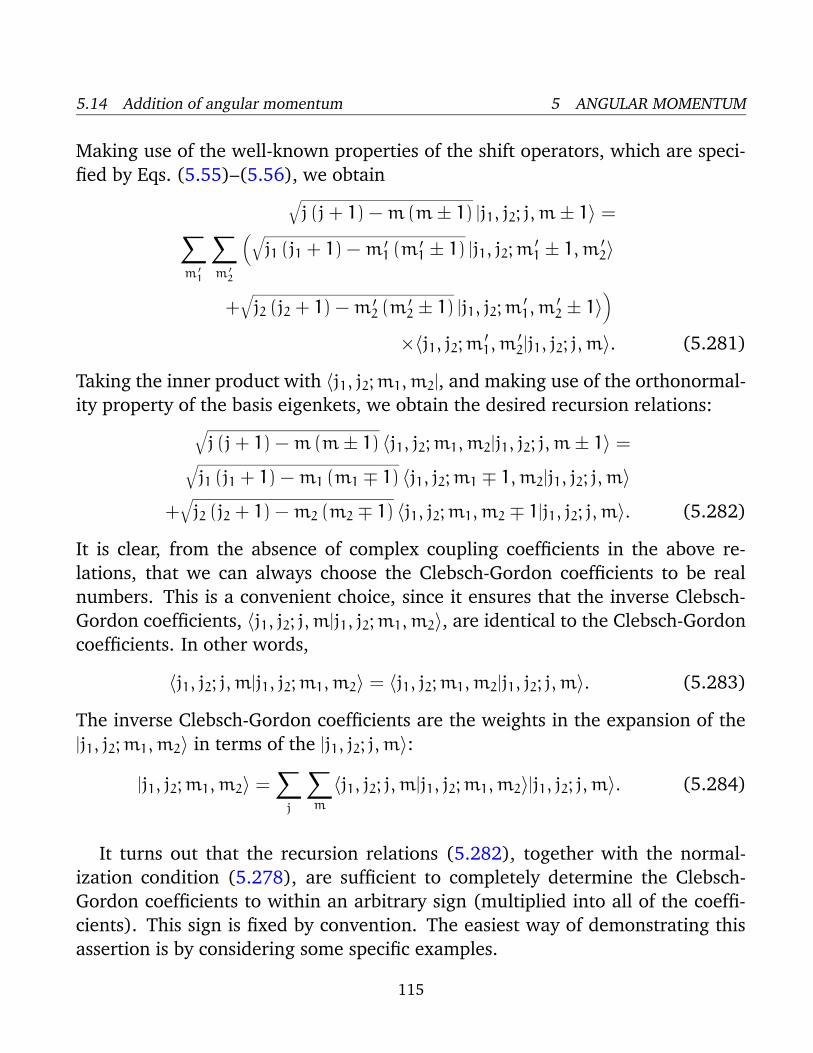
5.14 Addition of angular momentum 5 ANGULAR MOMENTUM
Making use of the well-known properties of the shift operators, which are speci-
fied by Eqs. (5.55)–(5.56), we obtain√
j (j+ 1) −m (m± 1) |j1, j2; j,m± 1〉 =∑
m ′
1
∑
m ′
2
(
√
j1 (j1 + 1) −m ′1 (m ′
1 ± 1) |j1, j2;m′1 ± 1,m ′
2〉
+√
j2 (j2 + 1) −m ′2 (m ′
2 ± 1) |j1, j2;m′1,m
′2 ± 1〉
)
×〈j1, j2;m ′1,m
′2|j1, j2; j,m〉. (5.281)
Taking the inner product with 〈j1, j2;m1,m2|, and making use of the orthonormal-
ity property of the basis eigenkets, we obtain the desired recursion relations:√
j (j+ 1) −m (m± 1) 〈j1, j2;m1,m2|j1, j2; j,m± 1〉 =√
j1 (j1 + 1) −m1 (m1 ∓ 1) 〈j1, j2;m1 ∓ 1,m2|j1, j2; j,m〉+√
j2 (j2 + 1) −m2 (m2 ∓ 1) 〈j1, j2;m1,m2 ∓ 1|j1, j2; j,m〉. (5.282)
It is clear, from the absence of complex coupling coefficients in the above re-
lations, that we can always choose the Clebsch-Gordon coefficients to be real
numbers. This is a convenient choice, since it ensures that the inverse Clebsch-
Gordon coefficients, 〈j1, j2; j,m|j1, j2;m1,m2〉, are identical to the Clebsch-Gordon
coefficients. In other words,
〈j1, j2; j,m|j1, j2;m1,m2〉 = 〈j1, j2;m1,m2|j1, j2; j,m〉. (5.283)
The inverse Clebsch-Gordon coefficients are the weights in the expansion of the
|j1, j2;m1,m2〉 in terms of the |j1, j2; j,m〉:
|j1, j2;m1,m2〉 =∑
j
∑
m
〈j1, j2; j,m|j1, j2;m1,m2〉|j1, j2; j,m〉. (5.284)
It turns out that the recursion relations (5.282), together with the normal-
ization condition (5.278), are sufficient to completely determine the Clebsch-
Gordon coefficients to within an arbitrary sign (multiplied into all of the coeffi-
cients). This sign is fixed by convention. The easiest way of demonstrating this
assertion is by considering some specific examples.
115
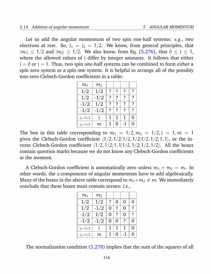
5.14 Addition of angular momentum 5 ANGULAR MOMENTUM
Let us add the angular momentum of two spin one-half systems: e.g., two
electrons at rest. So, j1 = j2 = 1/2. We know, from general principles, that
|m1| ≤ 1/2 and |m2| ≤ 1/2. We also know, from Eq. (5.276), that 0 ≤ j ≤ 1,
where the allowed values of j differ by integer amounts. It follows that either
j = 0 or j = 1. Thus, two spin one-half systems can be combined to form either a
spin zero system or a spin one system. It is helpful to arrange all of the possibly
non-zero Clebsch-Gordon coefficients in a table:
m1 m2
1/2 1/2 ? ? ? ?
1/2 -1/2 ? ? ? ?
-1/2 1/2 ? ? ? ?
-1/2 -1/2 ? ? ? ?
j1=1/2 j 1 1 1 0
j2=1/2 m 1 0 -1 0
The box in this table corresponding to m1 = 1/2,m2 = 1/2, j = 1,m = 1
gives the Clebsch-Gordon coefficient 〈1/2, 1/2; 1/2, 1/2|1/2, 1/2; 1, 1〉, or the in-
verse Clebsch-Gordon coefficient 〈1/2, 1/2; 1, 1|1/2, 1/2; 1/2, 1/2〉. All the boxes
contain question marks because we do not know any Clebsch-Gordon coefficients
at the moment.
A Clebsch-Gordon coefficient is automatically zero unless m1 + m2 = m. In
other words, the z-components of angular momentum have to add algebraically.
Many of the boxes in the above table correspond tom1+m2 6= m. We immediately
conclude that these boxes must contain zeroes: i.e.,
m1 m2
1/2 1/2 ? 0 0 0
1/2 -1/2 0 ? 0 ?
-1/2 1/2 0 ? 0 ?
-1/2 -1/2 0 0 ? 0
j1=1/2 j 1 1 1 0
j2=1/2 m 1 0 -1 0
The normalization condition (5.278) implies that the sum of the squares of all
116
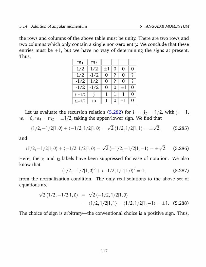
5.14 Addition of angular momentum 5 ANGULAR MOMENTUM
the rows and columns of the above table must be unity. There are two rows and
two columns which only contain a single non-zero entry. We conclude that these
entries must be ±1, but we have no way of determining the signs at present.
Thus,m1 m2
1/2 1/2 ±1 0 0 0
1/2 -1/2 0 ? 0 ?
-1/2 1/2 0 ? 0 ?
-1/2 -1/2 0 0 ±1 0
j1=1/2 j 1 1 1 0
j2=1/2 m 1 0 -1 0
Let us evaluate the recursion relation (5.282) for j1 = j2 = 1/2, with j = 1,
m = 0, m1 = m2 = ±1/2, taking the upper/lower sign. We find that
〈1/2,−1/2|1, 0〉 + 〈−1/2, 1/2|1, 0〉 =√2 〈1/2, 1/2|1, 1〉 = ±
√2, (5.285)
and
〈1/2,−1/2|1, 0〉 + 〈−1/2, 1/2|1, 0〉 =√2 〈−1/2,−1/2|1,−1〉 = ±
√2. (5.286)
Here, the j1 and j2 labels have been suppressed for ease of notation. We also
know that
〈1/2,−1/2|1, 0〉2 + 〈−1/2, 1/2|1, 0〉2 = 1, (5.287)
from the normalization condition. The only real solutions to the above set of
equations are√2 〈1/2,−1/2|1, 0〉 =
√2 〈−1/2, 1/2|1, 0〉
= 〈1/2, 1/2|1, 1〉 = 〈1/2, 1/2|1,−1〉 = ±1. (5.288)
The choice of sign is arbitrary—the conventional choice is a positive sign. Thus,
117
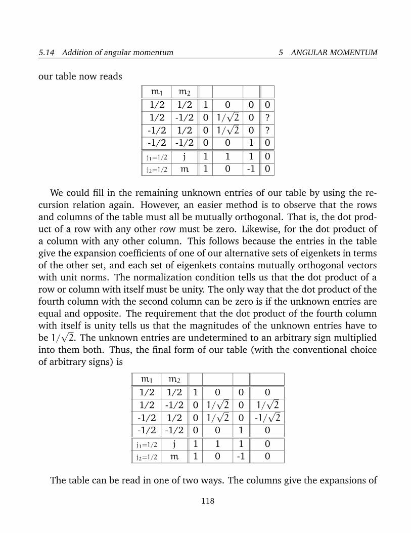
5.14 Addition of angular momentum 5 ANGULAR MOMENTUM
our table now reads
m1 m2
1/2 1/2 1 0 0 0
1/2 -1/2 0 1/√2 0 ?
-1/2 1/2 0 1/√2 0 ?
-1/2 -1/2 0 0 1 0
j1=1/2 j 1 1 1 0
j2=1/2 m 1 0 -1 0
We could fill in the remaining unknown entries of our table by using the re-
cursion relation again. However, an easier method is to observe that the rows
and columns of the table must all be mutually orthogonal. That is, the dot prod-
uct of a row with any other row must be zero. Likewise, for the dot product of
a column with any other column. This follows because the entries in the table
give the expansion coefficients of one of our alternative sets of eigenkets in terms
of the other set, and each set of eigenkets contains mutually orthogonal vectors
with unit norms. The normalization condition tells us that the dot product of a
row or column with itself must be unity. The only way that the dot product of the
fourth column with the second column can be zero is if the unknown entries are
equal and opposite. The requirement that the dot product of the fourth column
with itself is unity tells us that the magnitudes of the unknown entries have to
be 1/√2. The unknown entries are undetermined to an arbitrary sign multiplied
into them both. Thus, the final form of our table (with the conventional choice
of arbitrary signs) is
m1 m2
1/2 1/2 1 0 0 0
1/2 -1/2 0 1/√2 0 1/
√2
-1/2 1/2 0 1/√2 0 -1/
√2
-1/2 -1/2 0 0 1 0
j1=1/2 j 1 1 1 0
j2=1/2 m 1 0 -1 0
The table can be read in one of two ways. The columns give the expansions of
118
5.14 Addition of angular momentum 5 ANGULAR MOMENTUM
the eigenstates of overall angular momentum in terms of the eigenstates of the
individual angular momenta of the two component systems. Thus, the second
column tells us that
|1, 0〉 =1√2
( |1/2,−1/2〉 + | − 1/2, 1/2〉 ) . (5.289)
The ket on the left-hand side is a |j,m〉 ket, whereas those on the right-hand side
are |m1,m2〉 kets. The rows give the expansions of the eigenstates of individual
angular momentum in terms of those of overall angular momentum. Thus, the
second row tells us that
|1/2,−1/2〉 =1√2
( |1, 0〉 + |0, 0〉 ) . (5.290)
Here, the ket on the left-hand side is a |m1,m2〉 ket, whereas those on the right-
hand side are |j,m〉 kets.
Note that our table is really a combination of two sub-tables, one involving
j = 0 states, and one involving j = 1 states. The Clebsch-Gordon coefficients cor-
responding to two different choices of j are completely independent: i.e., there is
no recursion relation linking Clebsch-Gordon coefficients corresponding to differ-
ent values of j. Thus, for every choice of j1, j2, and j we can construct a table of
Clebsch-Gordon coefficients corresponding to the different allowed values of m1,
m2, and m (subject to the constraint that m1 +m2 = m). A complete knowledge
of angular momentum addition is equivalent to a knowing all possible tables of
Clebsch-Gordon coefficients. These tables are listed (for moderate values of j1, j2and j) in many standard reference books.
119
6 APPROXIMATION METHODS
6 Approximation methods
6.1 Introduction
We have developed techniques by which the general energy eigenvalue problem
can be reduced to a set of coupled partial differential equations involving various
wave-functions. Unfortunately, the number of such problems which yield exactly
soluble equations is comparatively small. Clearly, we need to develop some tech-
niques for finding approximate solutions to otherwise intractable problems.
Consider the following problem, which is very common. The Hamiltonian of a
system is written
H = H0 +H1. (6.1)
Here, H0 is a simple Hamiltonian for which we know the exact eigenvalues and
eigenstates. H1 introduces some interesting additional physics into the problem,
but it is sufficiently complicated that when we add it to H0 we can no longer
find the exact energy eigenvalues and eigenstates. However, H1 can, in some
sense (which we shall specify more exactly later on), be regarded as being small
compared to H0. Can we find the approximate eigenvalues and eigenstates of the
modified Hamiltonian, H0+H1, by performing some sort of perturbation analysis
about the eigenvalues and eigenstates of the original Hamiltonian, H0? Let us
investigate.
6.2 The two-state system
Let us begin by considering time-independent perturbation theory, in which the
modification to the Hamiltonian, H1, has no explicit dependence on time. It is
usually assumed that the unperturbed Hamiltonian, H0, is also time-independent.
Consider the simplest non-trivial system, in which there are only two indepen-
dent eigenkets of the unperturbed Hamiltonian. These are denoted
H0 |1〉 = E1 |1〉, (6.2)
120

6.2 The two-state system 6 APPROXIMATION METHODS
H0 |2〉 = E2 |2〉. (6.3)
It is assumed that these states, and their associated eigenvalues, are known. Since
H0 is, by definition, an Hermitian operator, its two eigenkets are orthonormal and
form a complete set. The lengths of these eigenkets are both normalized to unity.
Let us now try to solve the modified energy eigenvalue problem
(H0 +H1)|E〉 = E |E〉. (6.4)
In fact, we can solve this problem exactly. Since, the eigenkets of H0 form a
complete set, we can write
|E〉 = 〈1|E〉|1〉 + 〈2|E〉|2〉. (6.5)
Right-multiplication of Eq. (6.4) by 〈1| and 〈2| yields two coupled equations,
which can be written in matrix form:
E1 − E+ e11 e12e ∗12 E2 − E+ e22
〈1|E〉〈2|E〉
=
0
0
. (6.6)
Here,
e11 = 〈1|H1|1〉, (6.7)
e22 = 〈2|H1|2〉, (6.8)
e12 = 〈1|H1|2〉. (6.9)
In the special (but common) case of a perturbing Hamiltonian whose diagonal
matrix elements (in the unperturbed eigenstates) are zero, so that
e11 = e22 = 0, (6.10)
the solution of Eq. (6.6) (obtained by setting the determinant of the matrix equal
to zero) is
E =(E1 + E2) ±
√
(E1 − E2)2 + 4 |e12|2
2. (6.11)
Let us expand in the supposedly small parameter
ε =|e12|
|E1 − E2|. (6.12)
121
6.3 Non-degenerate perturbation theory 6 APPROXIMATION METHODS
We obtain
E ' 1
2(E1 + E2) ±
1
2(E1 − E2)(1+ 2 ε2 + · · ·). (6.13)
The above expression yields the modifications to the energy eigenvalues due to
the perturbing Hamiltonian:
E ′1 = E1 +
|e12|2
E1 − E2+ · · · , (6.14)
E ′2 = E2 −
|e12|2
E1 − E2+ · · · . (6.15)
Note that H1 causes the upper eigenvalue to rise, and the lower eigenvalue to
fall. It is easily demonstrated that the modified eigenkets take the form
|1〉 ′ = |1〉 +e ∗12
E1 − E2|2〉 + · · · , (6.16)
|2〉 ′ = |2〉 −e12
E1 − E2|1〉 + · · · . (6.17)
Thus, the modified energy eigenstates consist of one of the unperturbed eigen-
states with a slight admixture of the other. Note that the series expansion in
Eq. (6.13) only converges if 2 |ε| < 1. This suggests that the condition for the
validity of the perturbation expansion is
|e12| <|E1 − E2|
2. (6.18)
In other words, when we say that H1 needs to be small compared to H0, what we
really mean is that the above inequality needs to be satisfied.
6.3 Non-degenerate perturbation theory
Let us now generalize our perturbation analysis to deal with systems possessing
more than two energy eigenstates. The energy eigenstates of the unperturbed
Hamiltonian, H0, are denoted
H0 |n〉 = En |n〉, (6.19)
122
6.3 Non-degenerate perturbation theory 6 APPROXIMATION METHODS
where n runs from 1 to N. The eigenkets |n〉 are orthonormal, form a complete
set, and have their lengths normalized to unity. Let us now try to solve the energy
eigenvalue problem for the perturbed Hamiltonian:
(H0 +H1)|E〉 = E |E〉. (6.20)
We can express |E〉 as a linear superposition of the unperturbed energy eigenkets,
|E〉 =∑
k
〈k|E〉|k〉, (6.21)
where the summation is from k = 1 to N. Substituting the above equation into
Eq. (6.20), and right-multiplying by 〈m|, we obtain
(Em + emm − E)〈m|E〉 +∑
k6=memk〈k|E〉 = 0, (6.22)
where
emk = 〈m|H1|k〉. (6.23)
Let us now develop our perturbation expansion. We assume that
|emk|
Em − Ek∼ O(ε), (6.24)
for all m 6= k, where ε 1 is our expansion parameter. We also assume that
|emm|
Em∼ O(ε), (6.25)
for all m. Let us search for a modified version of the nth unperturbed energy
eigenstate, for which
E = En +O(ε), (6.26)
and
〈n|E〉 = 1, (6.27)
〈m|E〉 ∼ O(ε), (6.28)
for m 6= n. Suppose that we write out Eq. (6.22) for m 6= n, neglecting terms
which are O(ε2) according to our expansion scheme. We find that
(Em − En)〈m|E〉 + emn ' 0, (6.29)
123
6.4 The quadratic Stark effect 6 APPROXIMATION METHODS
giving
〈m|E〉 ' −emn
Em − En. (6.30)
Substituting the above expression into Eq. (6.22), evaluated for m = n, and
neglecting O(ε3) terms, we obtain
(En + enn − E) −∑
k6=n
|enk|2
Ek − En= 0. (6.31)
Thus, the modified nth energy eigenstate possesses an eigenvalue
E ′n = En + enn +
∑
k6=n
|enk|2
En − Ek+O(ε3), (6.32)
and a eigenket
|n〉 ′ = |n〉 +∑
k6=n
ekn
En − Ek|k〉 +O(ε2). (6.33)
Note that
〈m|n〉 ′ = δmn +e∗nm
Em − En+
emn
En − Em+O(ε2) = δmn +O(ε2). (6.34)
Thus, the modified eigenkets remain orthonormal and properly normalized to
O(ε2).
6.4 The quadratic Stark effect
Suppose that a one-electron atom [i.e., either a hydrogen atom, or an alkali metal
atom (which possesses one valance electron orbiting outside a closed, spher-
ically symmetric shell)] is subjected to a uniform electric field in the positive
z-direction. The Hamiltonian of the system can be split into two parts. The un-
perturbed Hamiltonian,
H0 =p2
2me
+ V(r), (6.35)
and the perturbing Hamiltonian,
H1 = e |E| z. (6.36)
124

6.4 The quadratic Stark effect 6 APPROXIMATION METHODS
It is assumed that the unperturbed energy eigenvalues and eigenstates are
completely known. The electron spin is irrelevant in this problem (since the spin
operators all commute with H1), so we can ignore the spin degrees of freedom of
the system. This implies that the system possesses no degenerate energy eigen-
values. This is not true for the n 6= 1 energy levels of the hydrogen atom, due to
the special properties of a pure Coulomb potential. It is necessary to deal with
this case separately, because the perturbation theory presented in Sect. 6.3 breaks
down for degenerate unperturbed energy levels.
An energy eigenket of the unperturbed Hamiltonian is characterized by three
quantum numbers—the radial quantum number n, and the two angular quantum
numbers l and m (see Sect. 5.6). Let us denote such a ket |n, l,m〉, and let its
energy level be Enlm. According to Eq. (6.32), the change in this energy level
induced by a small electric field is given by
∆Enlm = e |E| 〈n, l,m|z|n, l,m〉
+e2 |E|2∑
n ′,l ′,m ′ 6=n,l,m
|〈n, l,m|z|n, ′ l ′,m ′〉|2Enlm − En ′l ′m ′
. (6.37)
Now, since
Lz = xpy − ypx, (6.38)
it follows that
[Lz, z] = 0. (6.39)
Thus,
〈n, l,m|[Lz, z]|n′, l ′,m ′〉 = 0, (6.40)
giving
(m−m ′)〈n, l,m|z|n ′, l ′,m ′〉 = 0, (6.41)
since |n, l,m〉 is, by definition, an eigenstate of Lz with eigenvalue m h. It is
clear, from the above relation, that the matrix element 〈n, l,m|z|n ′, l ′,m ′〉 is zero
unless m ′ = m. This is termed the selection rule for the quantum number m.
Let us now determine the selection rule for l. We have
[L2, z] = [L 2x , z] + [L 2y , z]
125
6.4 The quadratic Stark effect 6 APPROXIMATION METHODS
= Lx[Lx, z] + [Lx, z]Lx + Ly[Ly, z] + [Ly, z]Ly
= i h (−Lx y− yLx + Ly x+ x Ly)
= 2 i h (Ly x− Lx y+ i h z)
= 2 i h (Ly x− yLx) = 2 i h (x Ly − Lx y), (6.42)
where use has been made of Eqs. (5.1)–(5.6). Similarly,
[L2, y] = 2 i h (Lx z− x Lz), (6.43)
[L2, x] = 2 i h (yLz − Ly z). (6.44)
Thus,
[L2, [L2, z]] = 2 i h(
L2, Ly x− Lx y+ i h z)
= 2 i h(
Ly[L2, x] − Lx[L
2, y] + i h [L2, z])
,
= −4 h2 Ly(yLz − Ly z) + 4 h2 Lx(Lx z− x Lz)
−2 h2(L2 z− z L2). (6.45)
This reduces to
[L2, [L2, z]] = −h2[
4 (Lx x+ Ly y+ Lz z)Lz − 4 (L 2x + L 2y + L 2z ) z
+2 (L2 z− z L2)]
. (6.46)
However, it is clear from Eqs. (5.1)–(5.3) that
Lx x+ Ly y+ Lz z = 0. (6.47)
Hence, we obtain
[L2, [L2, z]] = 2 h2 (L2 z+ z L2). (6.48)
Finally, the above expression expands to give
L4 z− 2 L2 z L2 + z L4 − 2 h2(L2 z+ z L2) = 0. (6.49)
Equation (6.49) implies that
〈n, l,m|L4 z− 2 L2 z L2 + z L4 − 2 h2 (L2 z+ z L2)|n ′, l ′,m ′〉 = 0. (6.50)
126
6.4 The quadratic Stark effect 6 APPROXIMATION METHODS
This expression yields[
l2 (l+ 1)2 − 2 l (l+ 1) l ′ (l ′ + 1) + l ′2 (l ′ + 1)2
−2 l (l+ 1) − 2 l ′ (l ′ + 1)] 〈n, l,m|z|n ′, l ′,m ′〉 = 0, (6.51)
which reduces to
(l+ l ′ + 2) (l+ l ′) (l− l ′ + 1) (l− l ′ − 1)〈n, l,m|z|n ′, l ′,m ′〉 = 0. (6.52)
According to the above formula, the matrix element 〈n, l,m|z|n ′, l ′,m ′〉 vanishes
unless l = l ′ = 0 or l ′ = l± 1. This matrix element can be written
〈n, l,m|z|n ′, l ′,m ′〉 =
∫∫∫
ψ∗nlm(r ′, θ ′, ϕ ′) r ′ cos θ ′ψn ′m ′l ′(r
′, θ ′, ϕ ′)dV ′, (6.53)
where ψnlm(r ′) = 〈r ′|n, l,m〉. Recall, however, that the wave-function of an l = 0
state is spherically symmetric (see Sect. 5.3): i.e., ψn00(r′) = ψn00(r
′). It follows
from Eq. (6.53) that the matrix element vanishes by symmetry when l = l ′ = 0.
In conclusion, the matrix element 〈n, l,m|z|n ′, l ′,m ′〉 is zero unless l ′ = l ± 1.This is the selection rule for the quantum number l.
Application of the selection rules to Eq. (6.37) yields
∆Enlm = e2 |E|2∑
n ′
∑
l ′=l±1
|〈n, l,m|z|n ′, l ′,m〉|2Enlm − En ′l ′m
. (6.54)
Note that all of the terms in Eq. (6.37) which vary linearly with the electric field-
strength vanish by symmetry, according to the selection rules. Only those terms
which vary quadratically with the field-strength survive. The polarizability of an
atom is defined in terms of the energy-shift of the atomic state as follows:
∆E = −1
2α |E|2. (6.55)
Consider the ground state of a hydrogen atom. (Recall, that we cannot address
the n > 1 excited states because they are degenerate, and our theory cannot
handle this at present). The polarizability of this state is given by
α = 2 e2∑
n>1
|〈1, 0, 0|z|n, 1, 0〉|2En00 − E100
. (6.56)
127
6.4 The quadratic Stark effect 6 APPROXIMATION METHODS
Here, we have made use of the fact that En10 = En00 for a hydrogen atom.
The sum in the above expression can be evaluated approximately by noting
that [see Eq. (5.120)]
En00 = −e2
8πε0 a0 n2(6.57)
for a hydrogen atom, where
a0 =4πε0 h
2
µe2= 5.3× 10⁻¹¹ meters (6.58)
is the Bohr radius. We can write
En00 − E100 ≥ E200 − E100 =3
4
e2
8πε0 a0. (6.59)
Thus,
α <16
34πε0 a0
∑
n>1
|〈1, 0, 0|z|n, 1, 0〉|2. (6.60)
However,∑
n>1
|〈1, 0, 0|z|n, 1, 0〉|2 =∑
n ′,l ′,m ′
〈1, 0, 0|z|n ′, l ′,m ′〉〈n ′,m ′, l ′|z|1, 0, 0〉
= 〈1, 0, 0|z2|1, 0, 0〉, (6.61)
where we have made use of the fact that the wave-functions of a hydrogen atom
form a complete set. It is easily demonstrated from the actual form of the ground
state wave-function that
〈1, 0, 0|z2|1, 0, 0〉 = a 20 . (6.62)
Thus, we conclude that
α <16
34πε0 a
30 ' 5.3 4πε0 a 3
0 . (6.63)
The true result is
α =9
24πε0 a
30 = 4.5 4πε0 a
30 . (6.64)
It is actually possible to obtain this answer, without recourse to perturbation the-
ory, by solving Schrodinger’s equation exactly in parabolic coordinates.
128
6.5 Degenerate perturbation theory 6 APPROXIMATION METHODS
6.5 Degenerate perturbation theory
Let us now consider systems in which the eigenstates of the unperturbed Hamil-
tonian, H0, possess degenerate energy levels. It is always possible to represent
degenerate energy eigenstates as the simultaneous eigenstates of the Hamilto-
nian and some other Hermitian operator (or group of operators). Let us denote
this operator (or group of operators) L. We can write
H0 |n, l〉 = En |n, l〉, (6.65)
and
L |n, l〉 = Lnl |n, l〉, (6.66)
where [H0, L] = 0. Here, the En and the Lnl are real numbers which depend on
the quantum numbers n, and n and l, respectively. It is always possible to find a
sufficient number of operators which commute with the Hamiltonian in order to
ensure that the Lnl are all different. In other words, we can choose L such that
the quantum numbers n and l uniquely specify each eigenstate. Suppose that for
each value of n there are Nn different values of l: i.e., the nth energy eigenstate
is Nn-fold degenerate.
In general, L does not commute with the perturbing Hamiltonian, H1. This
implies that the modified energy eigenstates are not eigenstates of L. In this situ-
ation, we expect the perturbation to split the degeneracy of the energy levels, so
that each modified eigenstate |n, l〉 ′ acquires a unique energy eigenvalue E ′nl. Let
us naively attempt to use the standard perturbation theory of Sect. 6.3 to evalu-
ate the modified energy eigenstates and energy levels. A direct generalization of
Eqs. (6.32) and (6.33) yields
E ′nl = En + enlnl +
∑
n ′,l ′ 6=n,l
|en ′l ′nl|2
En − En ′
+O(ε3), (6.67)
and
|n, l〉 ′ = |n, l〉 +∑
n ′,l ′ 6=n,l
en ′l ′nl
En − En ′
|n ′, l ′〉 +O(ε2), (6.68)
where
en ′l ′nl = 〈n ′, l ′|H1|n, l〉. (6.69)
129
6.5 Degenerate perturbation theory 6 APPROXIMATION METHODS
It is fairly obvious that the summations in Eqs. (6.67) and (6.68) are not well-
behaved if the nth energy level is degenerate. The problem terms are those
involving unperturbed eigenstates labeled by the same value of n, but different
values of l: i.e., those states whose unperturbed energies are En. These terms
give rise to singular factors 1/(En − En) in the summations. Note, however, that
this problem would not exist if the matrix elements, enl ′nl, of the perturbing
Hamiltonian between distinct, degenerate, unperturbed energy eigenstates cor-
responding to the eigenvalue En were zero. In other words, if
〈n, l ′|H1|n, l〉 = λnl δll ′, (6.70)
then all of the singular terms in Eqs. (6.67) and (6.68) would vanish.
In general, Eq. (6.70) is not satisfied. Fortunately, we can always redefine the
unperturbed energy eigenstates belonging to the eigenvalue En in such a manner
that Eq. (6.70) is satisfied. Let us defineNn new states which are linear combina-
tions of the Nn original degenerate eigenstates corresponding to the eigenvalue
En:
|n, l(1)〉 =
Nn∑
k=1
〈n, k|n, l(1)〉|n, k〉. (6.71)
Note that these new states are also degenerate energy eigenstates of the unper-
turbed Hamiltonian corresponding to the eigenvalue En. The |n, l(1)〉 are chosen
in such a manner that they are eigenstates of the perturbing Hamiltonian, H1.
Thus,
H1 |n, l(1)〉 = λnl |n, l(1)〉. (6.72)
The |n, l(1)〉 are also chosen so that they are orthonormal, and have unit lengths.
It follows that
〈n, l ′(1)|H1|n, l(1)〉 = λnl δll ′. (6.73)
Thus, if we use the new eigenstates, instead of the old ones, then we can employ
Eqs. (6.67) and (6.68) directly, since all of the singular terms vanish. The only
remaining difficulty is to determine the new eigenstates in terms of the original
ones.
130
6.5 Degenerate perturbation theory 6 APPROXIMATION METHODS
NowNn∑
l=1
|n, l〉〈n, l| = 1, (6.74)
where 1 denotes the identity operator in the sub-space of all unperturbed energy
eigenkets corresponding to the eigenvalue En. Using this completeness relation,
the operator eigenvalue equation (6.72) can be transformed into a straightfor-
ward matrix eigenvalue equation:
Nn∑
l ′′=1
〈n, l ′|H1|n, l ′′〉〈n, l ′′|n, l(1)〉 = λnl 〈n, l ′|n, l(1)〉. (6.75)
This can be written more transparently as
U x = λ x, (6.76)
where the elements of the Nn ×Nn Hermitian matrix U are
Ujk = 〈n, j|H1|n, k〉. (6.77)
Provided that the determinant of U is non-zero, Eq. (6.76) can always be solved
to give Nn eigenvalues λnl (for l = 1 to Nn), with Nn corresponding eigenvectors
xnl. The eigenvectors specify the weights of the new eigenstates in terms of the
original eigenstates: i.e.,
(xnl)k = 〈n, k|n, l(1)〉, (6.78)
for k = 1 to Nn. In our new scheme, Eqs. (6.67) and (6.68) yield
E ′nl = En + λnl +
∑
n ′ 6=n,l ′
|en ′l ′nl|2
En − En ′
+O(ε3), (6.79)
and
|n, l(1)〉 ′ = |n, l(1)〉 +∑
n ′ 6=n,l ′
en ′l ′nl
En − En ′
|n ′, l ′〉 +O(ε2). (6.80)
There are no singular terms in these expressions, since the summations are over
n ′ 6= n: i.e., they specifically exclude the problematic, degenerate, unperturbed
energy eigenstates corresponding to the eigenvalue En. Note that the first-order
energy shifts are equivalent to the eigenvalues of the matrix equation (6.76).
131
6.6 The linear Stark effect 6 APPROXIMATION METHODS
6.6 The linear Stark effect
Let us examine the effect of an electric field on the excited energy levels of a
hydrogen atom. For instance, consider the n = 2 states. There is a single l =
0 state, usually referred to as 2s, and three l = 1 states (with m = −1, 0, 1),
usually referred to as 2p. All of these states possess the same energy, E200 =
−e2/(32π ε0 a0). As in Sect. 6.4, the perturbing Hamiltonian is
H1 = e |E| z. (6.81)
In order to apply perturbation theory, we have to solve the matrix eigenvalue
equation
U x = λ x, (6.82)
where U is the array of the matrix elements of H1 between the degenerate 2s and
2p states. Thus,
U = e |E|
0 〈2, 0, 0|z|2, 1, 0〉 0 0
〈2, 1, 0|z|2, 0, 0〉 0 0 0
0 0 0 0
0 0 0 0
, (6.83)
where the rows and columns correspond to the |2, 0, 0〉, |2, 1, 0〉, |2, 1, 1〉, and
|2, 1,−1〉 states, respectively. Here, we have made use of the selection rules,
which tell us that the matrix element of z between two hydrogen atom states is
zero unless the states possess the samem quantum number, and l quantum num-
bers which differ by unity. It is easily demonstrated, from the exact forms of the
2s and 2p wave-functions, that
〈2, 0, 0|z|2, 1, 0〉 = 〈2, 1, 0|z|2, 0, 0〉 = 3 a0. (6.84)
It can be seen, by inspection, that the eigenvalues of U are λ1 = 3 e a0 |E|,
λ2 = −3 e a0 |E|, λ3 = 0, and λ4 = 0. The corresponding eigenvectors are
x1 =
1/√2
1/√2
0
0
, (6.85)
132
6.6 The linear Stark effect 6 APPROXIMATION METHODS
x2 =
1/√2
−1/√2
0
0
, (6.86)
x3 =
0
0
1
0
, (6.87)
x4 =
0
0
0
1
. (6.88)
It follows from Sect. 6.5 that the simultaneous eigenstates of the unperturbed
Hamiltonian and the perturbing Hamiltonian take the form
|1〉 =|2, 0, 0〉 + |2, 1, 0〉√
2, (6.89)
|2〉 =|2, 0, 0〉 − |2, 1, 0〉√
2, (6.90)
|3〉 = |2, 1, 1〉, (6.91)
|4〉 = |2, 1,−1〉. (6.92)
In the absence of an electric field, all of these states possess the same energy, E200.
The first-order energy shifts induced by an electric field are given by
∆E1 = +3 e a0 |E|, (6.93)
∆E2 = −3 e a0 |E|, (6.94)
∆E3 = 0, (6.95)
∆E4 = 0. (6.96)
Thus, the energies of states 1 and 2 are shifted upwards and downwards, respec-
tively, by an amount 3 e a0 |E| in the presence of an electric field. States 1 and
2 are orthogonal linear combinations of the original 2s and 2p(m = 0) states.
133
6.7 Fine structure 6 APPROXIMATION METHODS
Note that the energy shifts are linear in the electric field-strength, so this is a
much larger effect that the quadratic effect described in Sect. 6.4. The energies
of states 3 and 4 (which are equivalent to the original 2p(m = 1) and 2p(m = −1)
states, respectively) are not affected to first-order. Of course, to second-order the
energies of these states are shifted by an amount which depends on the square of
the electric field-strength.
Note that the linear Stark effect depends crucially on the degeneracy of the 2s
and 2p states. This degeneracy is a special property of a pure Coulomb potential,
and, therefore, only applies to a hydrogen atom. Thus, alkali metal atoms do not
exhibit the linear Stark effect.
6.7 Fine structure
Let us now consider the energy levels of hydrogen-like atoms (i.e., alkali metal
atoms) in more detail. The outermost electron moves in a spherically symmetric
potential V(r) due to the nuclear charge and the charges of the other electrons
(which occupy spherically symmetric closed shells). The shielding effect of the
inner electrons causes V(r) to depart from the pure Coulomb form. This splits the
degeneracy of states characterized by the same value of n, but different values of
l. In fact, higher l states have higher energies.
Let us examine a phenomenon known as fine structure, which is due to inter-
action between the spin and orbital angular momenta of the outermost electron.
This electron experiences an electric field
E =∇Ve. (6.97)
However, a charge moving in an electric field also experiences an effective mag-
netic field
B = −v × E. (6.98)
Now, an electron possesses a spin magnetic moment [see Eq. (5.170)]
µ = −eS
me
. (6.99)
134
6.7 Fine structure 6 APPROXIMATION METHODS
We, therefore, expect a spin-orbit contribution to the Hamiltonian of the form
HLS = −µ·B
= −eS
me
· v ×(
1
e
r
r
dV
dr
)
=1
m 2e r
dV
drL·S, (6.100)
where L = me r×v is the orbital angular momentum. When the above expression
is compared to the observed spin-orbit interaction, it is found to be too large by
a factor of two. There is a classical explanation for this, due to spin precession,
which we need not go into. The correct quantum mechanical explanation requires
a relativistically covariant treatment of electron dynamics (this is achieved using
the so-called Dirac equation).
Let us now apply perturbation theory to a hydrogen-like atom, using HLS as
the perturbation (with HLS taking one half of the value given above), and
H0 =p2
2me
+ V(r) (6.101)
as the unperturbed Hamiltonian. We have two choices for the energy eigenstates
of H0. We can adopt the simultaneous eigenstates of H0, L2, S2, Lz and Sz, or the
simultaneous eigenstates of H0, L2, S 2, J 2, and Jz, where J = L + S is the total
angular momentum. Although the departure of V(r) from a pure 1/r form splits
the degeneracy of same n, different l, states, those states characterized by the
same values of n and l, but different values of ml, are still degenerate. (Here,
ml,ms, and mj are the quantum numbers corresponding to Lz, Sz, and Jz, respec-
tively.) Moreover, with the addition of spin degrees of freedom, each state is
doubly degenerate due to the two possible orientations of the electron spin (i.e.,
ms = ±1/2). Thus, we are still dealing with a highly degenerate system. We
know, from Sect. 6.6, that the application of perturbation theory to a degenerate
system is greatly simplified if the basis eigenstates of the unperturbed Hamilto-
nian are also eigenstates of the perturbing Hamiltonian. Now, the perturbing
Hamiltonian, HLS, is proportional to L·S, where
L·S =J 2 − L2 − S 2
2. (6.102)
135
6.7 Fine structure 6 APPROXIMATION METHODS
It is fairly obvious that the first group of operators (H0, L2, S2, Lz and Sz) does not
commute with HLS, whereas the second group (H0, L2, S 2, J 2, and Jz) does. In
fact, L·S is just a combination of operators appearing in the second group. Thus,
it is advantageous to work in terms of the eigenstates of the second group of
operators, rather than those of the first group.
We now need to find the simultaneous eigenstates of H0, L2, S 2, J 2, and Jz. This
is equivalent to finding the eigenstates of the total angular momentum resulting
from the addition of two angular momenta: j1 = l, and j2 = s = 1/2. According
to Eq. (5.276), the allowed values of the total angular momentum are j = l+ 1/2
and j = l− 1/2. We can write
|l+ 1/2,m〉 = cosα |m− 1/2, 1/2〉 + sinα |m+ 1/2,−1/2〉, (6.103)
|l− 1/2,m〉 = − sinα |m− 1/2, 1/2〉 + cosα |m+ 1/2,−1/2〉. (6.104)
Here, the kets on the left-hand side are |j,mj〉 kets, whereas those on the right-
hand side are |ml,ms〉 kets (the j1, j2 labels have been dropped, for the sake of
clarity). We have made use of the fact that the Clebsch-Gordon coefficients are
automatically zero unless mj = ml +ms. We have also made use of the fact that
both the |j,mj〉 and |ml,ms〉 kets are orthonormal, and have unit lengths. We
now need to determine
cosα = 〈m− 1/2, 1/2|l+ 1/2,m〉, (6.105)
where the Clebsch-Gordon coefficient is written in 〈ml,ms|j,mj〉 form.
Let us now employ the recursion relation for Clebsch-Gordon coefficients,
Eq. (5.282), with j1 = l, j2 = 1/2, j = l + 1/2,m1 = m − 1/2,m2 = 1/2 (lower
sign). We obtain√
(l+ 1/2) (l+ 3/2) −m (m+ 1) 〈m− 1/2, 1/2|l+ 1/2,m〉=√
l (l+ 1) − (m− 1/2) (m+ 1/2) 〈m+ 1/2, 1/2|l+ 1/2,m+ 1〉, (6.106)
which reduces to
〈m− 1/2, 1/2|l+ 1/2,m〉 =
√
√
√
√
√
l+m+ 1/2
l+m+ 3/2〈m+ 1/2, 1/2|l+ 1/2,m+ 1〉. (6.107)
136

6.7 Fine structure 6 APPROXIMATION METHODS
We can use this formula to successively increase the value of ml. For instance,
〈m− 1/2, 1/2|l+ 1/2,m〉 =
√
√
√
√
√
l+m+ 1/2
l+m+ 3/2
√
√
√
√
√
l+m+ 3/2
l+m+ 5/2
×〈m+ 3/2, 1/2|l+ 1/2,m+ 2〉. (6.108)
This procedure can be continued until ml attains its maximum possible value, l.
Thus,
〈m− 1/2, 1/2|l+ 1/2,m〉 =
√
√
√
√
l+m+ 1/2
2 l+ 1〈l, 1/2|l+ 1/2, l+ 1/2〉. (6.109)
Consider the situation in which ml and m both take their maximum values,
l and 1/2, respectively. The corresponding value of mj is l + 1/2. This value is
possible when j = l+1/2, but not when j = l−1/2. Thus, the |ml,ms〉 ket |l, 1/2〉must be equal to the |j,mj〉 ket |l + 1/2, l + 1/2〉, up to an arbitrary phase-factor.
By convention, this factor is taken to be unity, giving
〈l, 1/2|l+ 1/2, l+ 1/2〉 = 1. (6.110)
It follows from Eq. (6.109) that
cosα = 〈m− 1/2, 1/2|l+ 1/2,m〉 =
√
√
√
√
l+m+ 1/2
2 l+ 1. (6.111)
Now,
sin2 α = 1−l+m+ 1/2
2 l+ 1=l−m+ 1/2
2 l+ 1. (6.112)
We now need to determine the sign of sinα. A careful examination of the
recursion relation, Eq. (5.282), shows that the plus sign is appropriate. Thus,
|l+ 1/2,m〉 =
√
√
√
√
l+m+ 1/2
2 l+ 1|m− 1/2, 1/2〉
+
√
√
√
√
l−m+ 1/2
2 l+ 1|m+ 1/2,−1/2〉, (6.113)
137
6.7 Fine structure 6 APPROXIMATION METHODS
|l− 1/2,m〉 = −
√
√
√
√
l−m+ 1/2
2 l+ 1|m− 1/2, 1/2〉
+
√
√
√
√
l+m+ 1/2
2 l+ 1|m+ 1/2,−1/2〉. (6.114)
It is convenient to define so called spin-angular functions using the Pauli two-
component formalism:
Y j=l±1/2,ml = ±√
√
√
√
l±m+ 1/2
2 l+ 1Ym−1/2l (θ,ϕ)χ+
+
√
√
√
√
l∓m+ 1/2
2 l+ 1Ym+1/2l (θ,ϕ)χ−
=1√2 l+ 1
±√
l±m+ 1/2 Ym−1/2l (θ,ϕ)
√
l∓m+ 1/2 Ym+1/2l (θ,ϕ)
. (6.115)
These functions are eigenfunctions of the total angular momentum for spin one-
half particles, just as the spherical harmonics are eigenfunctions of the orbital
angular momentum. A general wave-function for an energy eigenstate in a
hydrogen-like atom is written
ψnlm± = Rnl(r)Y j=l±1/2,m. (6.116)
The radial part of the wave-function, Rnl(r), depends on the radial quantum num-
ber n and the angular quantum number l. The wave-function is also labeled by
m, which is the quantum number associated with Jz. For a given choice of l, the
quantum number j (i.e., the quantum number associated with J 2) can take the
values l± 1/2.
The |l± 1/2,m〉 kets are eigenstates of L·S, according to Eq. (6.102). Thus,
L·S |j = l± 1/2,mj = m〉 =h2
2[j (j+ 1) − l (l+ 1) − 3/4] |j,m〉, (6.117)
giving
L·S |l+ 1/2,m〉 =l h2
2|l+ 1/2,m〉, (6.118)
L·S |l− 1/2,m〉 = −(l+ 1) h2
2|l− 1/2,m〉. (6.119)
138
6.7 Fine structure 6 APPROXIMATION METHODS
It follows that∫
(Y l+1/2,m)† L·SY l+1/2,m dΩ =l h2
2, (6.120)
∫
(Y l−1/2,m)† L·SY l−1/2,m dΩ = −(l+ 1) h2
2, (6.121)
where the integrals are over all solid angle.
Let us now apply degenerate perturbation theory to evaluate the shift in energy
of a state whose wave-function is ψnlm± due to the spin-orbit Hamiltonian HLS.
To first-order, the energy-shift is given by
∆Enlm± =
∫
(ψnlm±)†HLSψnlm± dV, (6.122)
where the integral is over all space. Equations (6.100) (remember the factor of
two), (6.116), and (6.120)–(6.121) yield
∆Enlm+ = +1
2m 2e
⟨
1
r
dV
dr
⟩
l h2
2, (6.123)
∆Enlm− = −1
2m 2e
⟨
1
r
dV
dr
⟩
(l+ 1) h2
2, (6.124)
where⟨
1
r
dV
dr
⟩
=
∫
(Rnl)∗ 1
r
dV
drRnl r
2 dr. (6.125)
Equations (6.123)–(6.124) are known as Lande’s interval rule.
Let us now apply the above result to the case of a sodium atom. In chemist’s
notation, the ground state is written
(1s)2(2s)2(2p)6(3s). (6.126)
The inner ten electrons effectively form a spherically symmetric electron cloud.
We are interested in the excitation of the eleventh electron from 3s to some
higher energy state. The closest (in energy) unoccupied state is 3p. This state
has a higher energy than 3s due to the deviations of the potential from the pure
139
6.8 The Zeeman effect 6 APPROXIMATION METHODS
Coulomb form. In the absence of spin-orbit interaction, there are six degenerate
3p states. The spin-orbit interaction breaks the degeneracy of these states. The
modified states are labeled (3p)1/2 and (3p)3/2, where the subscript refers to the
value of j. The four (3p)3/2 states lie at a slightly higher energy level than the two
(3p)1/2 states, because the radial integral (6.125) is positive. The splitting of the
(3p) energy levels of the sodium atom can be observed using a spectroscope. The
well-known sodium D line is associated with transitions between the 3p and 3s
states. The fact that there are two slightly different 3p energy levels (note that
spin-orbit coupling does not split the 3s energy levels) means that the sodium D
line actually consists of two very closely spaced spectroscopic lines. It is easily
demonstrated that the ratio of the typical spacing of Balmer lines to the splitting
brought about by spin-orbit interaction is about 1 : α2, where
α =e2
2 ε0 h c=
1
137(6.127)
is the fine structure constant. Note that Eqs. (6.123)–(6.124) are not entirely
correct, since we have neglected an effect (namely, the relativistic mass correction
of the electron) which is the same order of magnitude as spin-orbit coupling.
6.8 The Zeeman effect
Consider a hydrogen-like atom placed in a uniform z-directed magnetic field. The
change in energy of the outermost electron is
HB = −µ·B, (6.128)
where
µ = −e
2me
(L + 2S) (6.129)
is its magnetic moment, including both the spin and orbital contributions. Thus,
HB =eB
2me
(Lz + 2 Sz). (6.130)
Suppose that the energy-shifts induced by the magnetic field are much smaller
than those induced by spin-orbit interaction. In this situation, we can treat HB as
140
6.8 The Zeeman effect 6 APPROXIMATION METHODS
a small perturbation acting on the eigenstates of H0+HLS. Of course, these states
are the simultaneous eigenstates of J 2 and Jz. Let us consider one of these states,
labeled by the quantum numbers j and m, where j = l ± 1/2. From standard
perturbation theory, the first-order energy-shift in the presence of a magnetic
field is
∆Enlm± = 〈l± 1/2,m|HB|l± 1/2,m〉. (6.131)
Since
Lz + 2 Sz = Jz + Sz, (6.132)
we find that
∆Enlm± =eB
2me
(m h+ 〈l± 1/2,m|Sz|l± 1/2,m〉 ) . (6.133)
Now, from Eqs. (6.113)–(6.114),
|l± 1/2,m〉 = ±√
√
√
√
l±m+ 1/2
2 l+ 1|m− 1/2, 1/2〉
+
√
√
√
√
l∓m+ 1/2
2 l+ 1|m+ 1/2,−1/2〉. (6.134)
It follows that
〈l± 1/2,m|Sz|l± 1/2,m〉 =h
2 (2 l+ 1)[(l±m+ 1/2) − (l∓m+ 1/2)]
= ± m h
2 l+ 1. (6.135)
Thus, we obtain Lande’s formula for the energy-shift induced by a weak magnetic
field:
∆Enlm± =e h B
2me
m
[
1± 1
2 l+ 1
]
. (6.136)
Let us apply this theory to the sodium atom. We have already seen that the
non-Coulomb potential splits the degeneracy of the 3s and 3p states, the latter
states acquiring a higher energy. The spin-orbit interaction splits the six 3p states
into two groups, with four j = 3/2 states lying at a slightly higher energy than
two j = 1/2 states. According to Eq. (6.136), a magnetic field splits the (3p)3/2
141
6.8 The Zeeman effect 6 APPROXIMATION METHODS
quadruplet of states, each state acquiring a different energy. In fact, the energy of
each state becomes dependent on the quantum number m, which measures the
projection of the total angular momentum along the z-axis. States with higher
m values have higher energies. A magnetic field also splits the (3p)1/2 doublet
of states. However, it is evident from Eq. (6.136) that these states are split by a
lesser amount than the j = 3/2 states.
Suppose that we increase the strength of the magnetic field, so that the energy-
shift due to the magnetic field becomes comparable to the energy-shift induced
by spin-orbit interaction. Clearly, in this situation, it does not make much sense to
think of HB as a small interaction term operating on the eigenstates of H0 +HLS.
In fact, this intermediate case is very difficult to analyze. Let us consider the
extreme limit in which the energy-shift due to the magnetic field greatly exceeds
that induced by spin-orbit effects. This is called the Paschen-Back limit.
In the Paschen-Back limit we can think of the spin-orbit Hamiltonian, HLS, as
a small interaction term operating on the eigenstates of H0 + HB. Note that the
magnetic Hamiltonian, HB, commutes with L2, S 2, Lz, Sz, but does not commute
with L2, S 2, J 2, Jz. Thus, in an intense magnetic field, the energy eigenstates of a
hydrogen-like atom are approximate eigenstates of the spin and orbital angular
momenta, but are not eigenstates of the total angular momentum. We can label
each state by the quantum numbers n (the energy quantum number), l, ml,
and ms. Thus, our energy eigenkets are written |n, l,ml,ms〉. The unperturbed
Hamiltonian, H0, causes states with different values of the quantum numbers n
and l to have different energies. However, states with the same value of n and l,
but different values of ml and ms, are degenerate. The shift in energy due to the
magnetic field is simply
∆Enlmlms= 〈n, l,ml,ms|HB|n, l,ml,ms〉
=e h B
2me
(ml + 2ms). (6.137)
Thus, states with different values of ml + 2ms acquire different energies.
Let us apply this result to a sodium atom. In the absence of a magnetic field,
the six 3p states form two groups of four and two states, depending on the values
142
6.8 The Zeeman effect 6 APPROXIMATION METHODS
of their total angular momentum. In the presence of an intense magnetic field
the 3p states are split into five groups. There is a state withml+2ms = 2, a state
with ml + 2ms = 1, two states with ml + 2ms = 0, a state with ml + 2ms = −1,
and a state with ml + 2ms = −2. These groups are equally spaced in energy, the
energy difference between adjacent groups being e h B/2me.
The energy-shift induced by the spin-orbit Hamiltonian is given by
∆Enlmlms= 〈n, l,ml,ms|HLS|n, l,ml,ms〉, (6.138)
where
HLS =1
2m 2e
1
r
dV
drL·S. (6.139)
Now,
〈L·S〉 = 〈Lz Sz + (L+ S− + L− S+)/2 〉= h2mlms, (6.140)
since
〈L±〉 = 〈S±〉 = 0 (6.141)
for expectation values taken between the simultaneous eigenkets of Lz and Sz.
Thus,
∆Enlmlms=h2mlms
2m 2e
⟨
1
r
dV
dr
⟩
. (6.142)
Let us apply the above result to a sodium atom. In the presence of an intense
magnetic field, the 3p states are split into five groups with (ml,ms) quantum
numbers (1, 1/2), (0, 1/2), (1,−1/2), or (−1, 1/2), (0,−1/2), and (−1,−1/2), re-
spectively, in order of decreasing energy. The spin-orbit term increases the en-
ergy of the highest energy state, does not affect the next highest energy state,
decreases, but does not split, the energy of the doublet, does not affect the next
lowest energy state, and increases the energy of the lowest energy state. The net
result is that the five groups of states are no longer equally spaced in energy.
The sort of magnetic field-strength needed to get into the Paschen-Bach limit
is given by
BPB ∼ α2eme
ε0 ha0' 25 tesla. (6.143)
143
6.9 Time-dependent perturbation theory 6 APPROXIMATION METHODS
Obviuously, this is an extremely large field-strength.
6.9 Time-dependent perturbation theory
Suppose that the Hamiltonian of the system under consideration can be written
H = H0 +H1(t), (6.144)
where H0 does not contain time explicitly, and H1 is a small time-dependent
perturbation. It is assumed that we are able to calculate the eigenkets of the
unperturbed Hamiltonian:
H0 |n〉 = En |n〉. (6.145)
We know that if the system is in one of the eigenstates of H0 then, in the ab-
sence of the external perturbation, it remains in this state for ever. However,
the presence of a small time-dependent perturbation can, in principle, give rise
to a finite probability that a system initially in some eigenstate |i〉 of the unper-
turbed Hamiltonian is found in some other eigenstate at a subsequent time (since
|i〉 is no longer an exact eigenstate of the total Hamiltonian), In other words, a
time-dependent perturbation causes the system to make transitions between its
unperturbed energy eigenstates. Let us investigate this effect.
Suppose that at t = t0 the state of the system is represented by
|A〉 =∑
n
cn |n〉, (6.146)
where the cn are complex numbers. Thus, the initial state is some linear su-
perposition of the unperturbed energy eigenstates. In the absence of the time-
dependent perturbation, the time evolution of the system is given by
|A, t0, t〉 =∑
n
cn exp([−iEn(t− t0)/h] |n〉. (6.147)
Now, the probability of finding the system in state |n〉 at time t is
Pn(t) = |cn exp[−iEn(t− t0)/h]|2 = |cn|2 = Pn(t0). (6.148)
144
6.9 Time-dependent perturbation theory 6 APPROXIMATION METHODS
Clearly, with H1 = 0, the probability of finding the system in state |n〉 at time t is
exactly the same as the probability of finding the system in this state at the initial
time t0. However, with H1 6= 0, we expect Pn(t) to vary with time. Thus, we can
write
|A, t0, t〉 =∑
n
cn(t) exp[−iEn(t− t0)/h] |n〉, (6.149)
where Pn(t) = |cn(t)|2. Here, we have carefully separated the fast phase oscilla-
tion of the eigenkets, which depends on the unperturbed Hamiltonian, from the
slow variation of the amplitudes cn(t), which depends entirely on the perturba-
tion (i.e., cn is constant if H1 = 0). Note that in Eq. (6.149) the eigenkets |n〉 are
time-independent (they are actually the eigenkets of H0 evaluated at the time t0).
Schrodinger’s time evolution equation yields
i h∂
∂t|A, t0, t〉 = H |A, t0, t〉 = (H0 +H1) |A, t0, t〉. (6.150)
It follows from Eq. (6.149) that
(H0 +H1)|A, t0, t〉 =∑
m
cm(t) exp[−iEm(t− t0)/h] (Em +H1) |m〉. (6.151)
We also have
i h∂
∂t|A, t0, t〉 =
∑
m
(
i hdcm
dt+ cm(t)Em
)
exp[−iEm(t− t0)/h] |m〉, (6.152)
where use has been made of the time-independence of the kets |m〉. According
to Eq. (6.150), we can equate the right-hand sides of the previous two equations
to obtain∑
m
i hdcm
dtexp[−iEm (t− t0)/h]|m〉 =
∑
m
cm(t) exp[−iEm(t− t0)/h]H1 |m〉.(6.153)
Left-multiplication by 〈n| yields
i hdcn
dt=∑
m
Hnm(t) exp[iωnm (t− t0)] cm(t), (6.154)
where
Hnm(t) = 〈n|H1(t)|m〉, (6.155)
145
6.10 The two-state system 6 APPROXIMATION METHODS
and
ωnm =En − Em
h. (6.156)
Here, we have made use of the standard orthonormality result, 〈n|m〉 = δnm.
Suppose that there are N linearly independent eigenkets of the unperturbed
Hamiltonian. According to Eq. (6.154), the time variation of the coefficients
cn, which specify the probability of finding the system in state |n〉 at time t, is de-
termined by N coupled first-order differential equations. Note that Eq. (6.154) is
exact—we have made no approximations at this stage. Unfortunately, we cannot
generally find exact solutions to this equation, so we have to obtain approximate
solutions via suitable expansions in small quantities. However, for the particu-
larly simple case of a two-state system (i.e., N = 2), it is actually possible to
solve Eq. (6.154) without approximation. This solution is of enormous practical
importance.
6.10 The two-state system
Consider a system in which the time-independent Hamiltonian possesses two
eigenstates, denoted
H0 |1〉 = E1 |1〉, (6.157)
H0 |2〉 = E2 |2〉. (6.158)
Suppose, for the sake of simplicity, that the diagonal matrix elements of the in-
teraction Hamiltonian, H1, are zero:
〈1|H1|1〉 = 〈2|H1|2〉 = 0. (6.159)
The off-diagonal matrix elements are assumed to oscillate sinusoidally at some
frequency ω:
〈1|H1|2〉 = 〈2|H1|1〉∗ = γ exp(iωt), (6.160)
where γ and ω are real. Note that it is only the off-diagonal matrix elements
which give rise to the effect which we are interested in—namely, transitions be-
tween states 1 and 2.
146
6.10 The two-state system 6 APPROXIMATION METHODS
For a two-state system, Eq. (6.154) reduces to
i hdc1
dt= γ exp[+i (ω−ω21) t ] c2, (6.161)
i hdc2
dt= γ exp[−i (ω−ω21) t ] c1, (6.162)
where ω21 = (E2 − E1)/h, and assuming that t0 = 0. Equations (6.161) and
(6.162) can be combined to give a second-order differential equation for the
time variation of the amplitude c2:
d2c2
dt2+ i (ω−ω21)
dc2
dt+γ2
h2c2 = 0. (6.163)
Once we have solved for c2, we can use Eq. (6.162) to obtain the amplitude c1.
Let us look for a solution in which the system is certain to be in state 1 at time
t = 0. Thus, our boundary conditions are c1(0) = 1 and c2(0) = 0. It is easily
demonstrated that the appropriate solutions are
c2(t) =−iγ/h
√
γ2/h2 + (ω−ω21)2/4exp[−i (ω−ω21) t/2]
× sin
(√
γ2/h2 + (ω−ω21)2/4 t
)
, (6.164)
c1(t) = exp[ i (ω−ω21) t/2] cos
(√
γ2/h2 + (ω−ω21)2/4 t
)
−i (ω−ω21)/2
√
γ2/h2 + (ω−ω21)2/4exp[ i (ω−ω21) t/2]
× sin
(√
γ2/h2 + (ω−ω21)2/4 t
)
. (6.165)
Now, the probability of finding the system in state 1 at time t is simply P1(t) =
|c1|2. Likewise, the probability of finding the system in state 2 at time t is P2(t) =
|c2|2. It follows that
P2(t) =γ2/h2
γ2/h2 + (ω−ω21)2/4
147
6.10 The two-state system 6 APPROXIMATION METHODS
× sin2(√
γ2/h2 + (ω−ω21)2/4 t
)
, (6.166)
P1(t) = 1− P2(t). (6.167)
This result is known as Rabi’s formula.
Equation (6.166) exhibits all the features of a classic resonance. At resonance,
when the oscillation frequency of the perturbation, ω, matches the frequency
ω21, we find that
P1(t) = cos2(γ t/h), (6.168)
P2(t) = sin2(γ t/h). (6.169)
According to the above result, the system starts off at t = 0 in state 1. After a
time interval π h/2 γ it is certain to be in state 2. After a further time interval
π h/2 γ it is certain to be in state 1, and so on. Thus, the system periodically
flip-flops between states 1 and 2 under the influence of the time-dependent per-
turbation. This implies that the system alternatively absorbs and emits energy
from the source of the perturbation.
The absorption-emission cycle also take place away from the resonance, when
ω 6= ω21. However, the amplitude of oscillation of the coefficient c2 is reduced.
This means that the maximum value of P2(t) is no longer unity, nor is the mini-
mum value of P1(t) zero. In fact, if we plot the maximum value of P2(t) as a func-
tion of the applied frequency, ω, we obtain a resonance curve whose maximum
(unity) lies at the resonance, and whose full-width half-maximum (in frequency)
is 4 γ/h. Thus, if the applied frequency differs from the resonant frequency by
substantially more than 2 γ/h then the probability of the system jumping from
state 1 to state 2 is very small. In other words, the time-dependent perturbation
is only effective at causing transitions between states 1 and 2 if its frequency of
oscillation lies in the approximate range ω21 ± 2 γ/h. Clearly, the weaker the
perturbation (i.e., the smaller γ becomes), the narrower the resonance.
148
6.11 Spin magnetic resonance 6 APPROXIMATION METHODS
6.11 Spin magnetic resonance
Consider a spin one-half system (e.g., a bound electron) placed in a uniform z-
directed magnetic field, and then subjected to a small time-dependent magnetic
field rotating in the x-y plane. Thus,
B = B0 z + B1(cosωt x + sinωt y), (6.170)
where B0 and B1 are constants, with B1 B0. The rotating magnetic field usu-
ally represents the magnetic component of an electromagnetic wave propagating
along the z-axis. In this system, the electric component of the wave has no effect.
The Hamiltonian is written
H = −µ·B = H0 +H1, (6.171)
where
H0 =eB0
me
Sz, (6.172)
and
H1 =eB1
me
(cosωtSx + sinωtSy) . (6.173)
The eigenstates of the unperturbed Hamiltonian are the ‘spin up’ and ‘spin
down’ states, denoted |+〉 and |−〉, respectively. Thus,
H0 |±〉 = ±e h B02me
|±〉. (6.174)
The time-dependent Hamiltonian can be written
H1 =eB1
2me
[
exp( iωt)S− + exp(−iωt)S+]
, (6.175)
where S+ and S− are the conventional raising and lowering operators for the spin
angular momentum. It follows that
〈+|H1|+〉 = 〈−|H1|−〉 = 0, (6.176)
and
〈−|H1|+〉 = 〈+|H1|−〉∗ =e h B1
2me
exp( iωt). (6.177)
149
6.12 The Dyson series 6 APPROXIMATION METHODS
It can be seen that this system is exactly the same as the two-state system
discussed in the previous section, provided that we make the identifications
|1〉 → |−〉, (6.178)
|2〉 → |+〉, (6.179)
ω21 →eB0
me
, (6.180)
γ →e h B1
2me
. (6.181)
The resonant frequency, ω21, is simply the spin precession frequency for an elec-
tron in a uniform magnetic field of strength B0. In the absence of the perturba-
tion, the expectation values of Sx and Sy oscillate because of the spin precession,
but the expectation value of Sz remains invariant. If we now apply a magnetic
perturbation rotating at the resonant frequency then, according to the analysis of
the previous section, the system undergoes a succession of spin-flops, |+〉 |−〉,in addition to the spin precession. We also know that if the oscillation frequency
of the applied field is very different from the resonant frequency then there is
virtually zero probability of the field triggering a spin-flop. The width of the
resonance (in frequency) is determined by the strength of the oscillating mag-
netic perturbation. Experimentalist are able to measure the magnetic moments
of electrons, and other spin one-half particles, to a high degree of accuracy by
placing the particles in a magnetic field, and subjecting them to an oscillating
magnetic field whose frequency is gradually scanned. By determining the reso-
nant frequency (i.e., the frequency at which the particles absorb energy from the
oscillating field), it is possible to calculate the magnetic moment.
6.12 The Dyson series
Let us now try to find approximate solutions of Eq. (6.154) for a general system.
It is convenient to work in terms of the time evolution operator, U(t0, t), which is
defined
|A, t0, t〉 = U(t0, t) |A〉. (6.182)
150
6.12 The Dyson series 6 APPROXIMATION METHODS
Here, |A, t0, t〉 is the state ket of the system at time t, given that the state ket at
the initial time t0 is |A〉. It is easily seen that the time evolution operator satisfies
the differential equation
i h∂U(t0, t)
∂t= (H0 +H1)U(t0, t), (6.183)
subject to the boundary condition
U(t0, t0) = 1. (6.184)
In the absence of the external perturbation, the time evolution operator re-
duces to
U(t0, t) = exp[−iH0(t− t0)/h]. (6.185)
Let us switch on the perturbation and look for a solution of the form
U(t0, t) = exp[−iH0(t− t0)/h]UI(t0, t). (6.186)
It is readily demonstrated that UI satisfies the differential equation
i h∂UI(t0, t)
∂t= HI(t0, t)UI(t0, t), (6.187)
where
HI(t0, t) = exp[+iH0(t− t0)/h]H1 exp[−iH0(t− t0)/h], (6.188)
subject to the boundary condition
UI(t0, t0) = 1. (6.189)
Note that UI specifies that component of the time evolution operator which is due
to the time-dependent perturbation. Thus, we would expect UI to contain all of
the information regarding transitions between different eigenstates of H0 caused
by the perturbation.
Suppose that the system starts off at time t0 in the eigenstate |i〉 of the un-
perturbed Hamiltonian. The subsequent evolution of the state ket is given by
Eq. (6.149),
|i, t0, t〉 =∑
m
cm(t) exp[−iEm(t− t0)/h] |m〉. (6.190)
151
6.12 The Dyson series 6 APPROXIMATION METHODS
However, we also have
|i, t0, t〉 = exp[−iH0(t− t0)/h]UI(t0, t) |i〉. (6.191)
It follows that
cn(t) = 〈n|UI(t0, t)|i〉, (6.192)
where use has been made of 〈n|m〉 = δnm. Thus, the probability that the system
is found in state |n〉 at time t, given that it is definitely in state |i〉 at time t0, is
simply
Pi→n(t0, t) = |〈n|UI(t0, t)|i〉|2. (6.193)
This quantity is usually termed the transition probability between states |i〉 and
|n〉.
Note that the differential equation (6.187), plus the boundary condition (6.189),
are equivalent to the following integral equation,
UI(t0, t) = 1−i
h
∫ t
t0
HI(t0, t′)UI(t0, t
′)dt ′. (6.194)
We can obtain an approximate solution to this equation by iteration:
UI(t0, t) ' 1−i
h
∫ t
t0
HI(t0, t′)
1−i
h
∫ t ′
t0
HI(t0, t′′)UI(t0, t
′′)
dt ′
' 1−i
h
∫ t
t0
HI(t0, t′)dt ′
+
(
−i
h
)2 ∫ t
t0
dt ′∫ t ′
t0
HI(t0, t′)HI(t0, t
′′)dt ′′ + · · · . (6.195)
This expansion is known as the Dyson series. Let
cn = c(0)n + c(1)
n + c(2)n + · · · , (6.196)
where the superscript (1) refers to a first-order term in the expansion, etc. It
follows from Eqs. (6.192) and (6.195) that
c(0)n (t) = δin, (6.197)
152
6.12 The Dyson series 6 APPROXIMATION METHODS
c(1)n (t) = −
i
h
∫ t
t0
〈n|HI(t0, t′)|i〉dt ′, (6.198)
c(2)n (t) =
(
−i
h
)2 ∫ t
t0
dt ′∫ t ′
t0
〈n|HI(t0, t′)HI(t0, t
′′)|i〉dt ′′. (6.199)
These expressions simplify to
c(0)n (t) = δin, (6.200)
c(1)n (t) = −
i
h
∫ t
t0
exp[ iωni (t′ − t0)]Hni(t
′)dt ′, (6.201)
c(2)n (t) =
(
−i
h
)2∑
m
∫ t
t0
dt ′∫ t ′
t0
dt ′′ exp[ iωnm (t ′ − t0)]
×Hnm(t ′) exp[ iωmi (t′′ − t0)]Hmi(t
′′), (6.202)
where
ωnm =En − Em
h, (6.203)
and
Hnm(t) = 〈n|H1(t)|m〉. (6.204)
The transition probability between states i and n is simply
Pi→n(t0, t) = |c(0)n + c(1)
n + c(2)n + · · · |2. (6.205)
According to the above analysis, there is no chance of a transition between
states |i〉 and |n〉 (i 6= n) to zeroth-order (i.e., in the absence of the perturbation).
To first-order, the transition probability is proportional to the time integral of the
matrix element 〈n|H1|i〉, weighted by some oscillatory phase-factor. Thus, if the
matrix element is zero, then there is no chance of a first-order transition between
states |i〉 and |n〉. However, to second-order, a transition between states |i〉 and
|n〉 is possible even when the matrix element 〈n|H1|i〉 is zero.
153
6.13 Constant perturbations 6 APPROXIMATION METHODS
6.13 Constant perturbations
Consider a constant perturbation which is suddenly switched on at time t = 0:
H1(t) = 0 for t < 0
H1(t) = H1 for t ≥ 0, (6.206)
where H1 is time-independent, but is generally a function of the position, mo-
mentum, and spin operators. Suppose that the system is definitely in state |i〉 at
time t = 0. According to Eqs. (6.200)–(6.202) (with t0 = 0),
c(0)n (t) = δin, (6.207)
c(1)n (t) = −
i
hHni
∫ t
0
exp[ iωni (t′ − t)]dt ′
=Hni
En − Ei[1− exp( iωni t)], (6.208)
giving
Pi→n(t) ' |c(1)n |2 =
4 |Hni|2
|En − Ei|2sin2
(En − Ei) t
2 h
, (6.209)
for i 6= n. The transition probability between states |i〉 and |n〉 can be written
Pi→n(t) =|Hni|
2 t2
h2sinc2
(En − Ei) t
2 h
, (6.210)
where
sinc(x) =sin x
x. (6.211)
The sinc function is highly oscillatory, and decays like 1/|x| at large |x|. It is a
good approximation to say that sinc(x) is small except when |x| <∼ π. It follows
that the transition probability, Pi→n, is small except when
|En − Ei| <∼
2π h
t. (6.212)
Note that in the limit t → ∞ only those transitions which conserve energy (i.e.,
En = Ei) have an appreciable probability of occurrence. At finite t, is is possible
to have transitions which do not exactly conserve energy, provided that
∆E∆t <∼ h, (6.213)
154
6.13 Constant perturbations 6 APPROXIMATION METHODS
where ∆E = |En − Ei| is change in energy of the system associated with the
transition, and ∆t = t is the time elapsed since the perturbation was switched
on. Clearly, this result is just a manifestation of the well-known uncertainty re-
lation for energy and time. This uncertainty relation is fundamentally different
to the position-momentum uncertainty relation, since in non-relativistic quan-
tum mechanics position and momentum are operators, whereas time is merely a
parameter.
The probability of a transition which conserves energy (i.e., En = Ei) is
Pi→n(t) =|Hin|
2 t2
h2, (6.214)
where use has been made of sinc(0) = 1. Note that this probability grows quadrat-
ically with time. This result is somewhat surprising, since it implies that the prob-
ability of a transition occurring in a fixed time interval, t to t+dt, grows linearly
with t, despite the fact that H1 is constant for t > 0. In practice, there is usually
a group of final states, all possessing nearly the same energy as the energy of the
initial state |i〉. It is helpful to define the density of states, ρ(E), where the num-
ber of final states lying in the energy range E to E+dE is given by ρ(E)dE. Thus,
the probability of a transition from the initial state i to any of the continuum of
possible final states is
Pi→(t) =
∫
Pi→n(t) ρ(En)dEn, (6.215)
giving
Pi→(t) =2 t
h
∫
|Hni|2 ρ(En) sinc2(x)dx, (6.216)
where
x = (En − Ei) t/2 h, (6.217)
and use has been made of Eq. (6.210). We know that in the limit t → ∞ the
function sinc(x) is only non-zero in an infinitesimally narrow range of final ener-
gies centred on En = Ei. It follows that, in this limit, we can take ρ(En) and |Hni|2
out of the integral in the above formula to obtain
Pi→[n](t) =2π
h|Hni|2 ρ(En) t
∣
∣
∣
∣
∣
En'Ei
, (6.218)
155
6.13 Constant perturbations 6 APPROXIMATION METHODS
where Pi→[n] denotes the transition probability between the initial state |i〉 and
all final states |n〉 which have approximately the same energy as the initial state.
Here, |Hni|2 is the average of |Hni|2 over all final states with approximately the
same energy as the initial state. In deriving the above formula, we have made
use of the result ∫∞
−∞
sinc2(x)dx = π. (6.219)
Note that the transition probability, Pi→[n], is now proportional to t, instead of t2.
It is convenient to define the transition rate, which is simply the transition
probability per unit time. Thus,
wi→[n] =dPi→[n]
dt, (6.220)
giving
wi→[n] =2π
h|Hni|2 ρ(En)
∣
∣
∣
∣
∣
En'Ei
. (6.221)
This appealingly simple result is known as Fermi’s golden rule. Note that the
transition rate is constant in time (for t > 0): i.e., the probability of a transition
occurring in the time interval t to t + dt is independent of t for fixed dt. Fermi’s
golden rule is sometimes written
wi→n =2π
h|Hni|
2 δ(En − E), (6.222)
where it is understood that this formula must be integrated with∫ρ(En)dEn to
obtain the actual transition rate.
Let us now calculate the second-order term in the Dyson series, using the
constant perturbation (6.206). From Eq. (6.202) we find that
c(2)n (t) =
(
−i
h
)2∑
m
HnmHmi
∫ t
0
dt ′ exp( iωnm t′ )
∫ t ′
0
dt ′′ exp( iωmi t )
=i
h
∑
m
HnmHmi
Em − Ei
∫ t
0
[exp( iωni t′ ) − exp( iωnm t
′] ) dt ′
=i t
h
∑
m
HnmHmi
Em − Ei[exp( iωni t/2) sinc(ωni t/2)
156
6.13 Constant perturbations 6 APPROXIMATION METHODS
− exp( iωnm t/2) sinc(ωnm t/2)] . (6.223)
Thus,
cn(t) = c(1)n + c(2)
n =i t
hexp( iωni t/2)
Hni +∑
m
HnmHmi
Em − Ei
sinc(ωni t/2)
−∑
m
HnmHmi
Em − Eiexp( iωim t/2) sinc(ωnm t/2)
, (6.224)
where use has been made of Eq. (6.208). It follows, by analogy with the previous
analysis, that
wi→[n] =2π
h
∣
∣
∣
∣
∣
∣
Hni +∑
m
HnmHmi
Em − Ei
∣
∣
∣
∣
∣
∣
2
ρ(En)
∣
∣
∣
∣
∣
∣
∣
En'Ei
, (6.225)
where the transition rate is calculated for all final states, |n〉, with approximately
the same energy as the initial state, |i〉, and for intermediate states, |m〉 whose
energies differ from that of the initial state. The fact that Em 6= Ei causes the
last term on the right-hand side of Eq. (6.224) to average to zero (due to the
oscillatory phase-factor) during the evaluation of the transition probability.
According to Eq. (6.225), a second-order transition takes place in two steps.
First, the system makes a non-energy-conserving transition to some intermedi-
ate state |m〉. Subsequently, the system makes another non-energy-conserving
transition to the final state |n〉. The net transition, from |i〉 to |n〉, conserves en-
ergy. The non-energy-conserving transitions are generally termed virtual transi-
tions, whereas the energy conserving first-order transition is termed a real transi-
tion. The above formula clearly breaks down if HnmHmi 6= 0 when Em = Ei.
This problem can be avoided by gradually turning on the perturbation: i.e.,
H1 → exp(η t)H1 (where η is very small). The net result is to change the en-
ergy denominator in Eq. (6.225) from Ei − Em to Ei − Em + i h η.
157
6.14 Harmonic perturbations 6 APPROXIMATION METHODS
6.14 Harmonic perturbations
Consider a perturbation which oscillates sinusoidally in time. This is usually
called a harmonic perturbation. Thus,
H1(t) = V exp( iωt) + V † exp(−iωt), (6.226)
where V is, in general, a function of position, momentum, and spin operators.
Let us initiate the system in the eigenstate |i〉 of the unperturbed Hamiltonian,
H0, and switch on the harmonic perturbation at t = 0. It follows from Eq. (6.201)
that
c(1)n =
−i
h
∫ t
0
[
Vni exp(iωt ′) + V†ni exp(−iωt ′)
]
exp( iωnit′)dt ′, (6.227)
=1
h
1− exp[ i (ωni +ω) t]
ωni +ωVni +
1− exp[ i (ωni −ω) t]
ωni −ωV
†ni
,
where
Vni = 〈n|V |i〉, (6.228)
V†ni = 〈n|V†|i〉 = 〈i|V |n〉∗. (6.229)
This formula is analogous to Eq. (6.208), provided that
ωni =En − Ei
h→ ωni ±ω. (6.230)
Thus, it follows from the previous analysis that the transition probability Pi→n(t) =
|c(1)n |2 is only appreciable in the limit t→∞ if
ωni +ω ' 0 or En ' Ei − hω, (6.231)
ωni −ω ' 0 or En ' Ei + hω. (6.232)
Clearly, (6.231) corresponds to the first term on the right-hand side of Eq. (6.227),
and (6.232) corresponds to the second term. The former term describes a process
by which the system gives up energy hω to the perturbing field, whilst making a
transition to a final state whose energy level is less than that of the initial state
158
6.15 Absorption and stimulated emission of radiation 6 APPROXIMATION METHODS
by hω. This process is known as stimulated emission. The latter term describes
a process by which the system gains energy hω from the perturbing field, whilst
making a transition to a final state whose energy level exceeds that of the initial
state by hω. This process is known as absorption. In both cases, the total energy
(i.e., that of the system plus the perturbing field) is conserved.
By analogy with Eq. (6.221),
wi→[n] =2π
h|Vni|2 ρ(En)
∣
∣
∣
∣
∣
En=Ei−hω
, (6.233)
wi→[n] =2π
h|V
†ni|2 ρ(En)
∣
∣
∣
∣
∣
En=Ei+hω
. (6.234)
Equation (6.233) specifies the transition rate for stimulated emission, whereas
Eq. (6.234) gives the transition rate for absorption. These equations are more
usually written
wi→n =2π
h|Vni|
2 δ(En − Ei + hω), (6.235)
wi→n =2π
h|V
†ni|2 δ(En − Ei − hω). (6.236)
It is clear from Eqs. (6.228)-(6.229) that |V†ni|2 = |Vni|
2. It follows from
Eqs. (6.233)–(6.234) thatwi→[n]
ρ(En)=wn→[i]
ρ(Ei). (6.237)
In other words, the rate of stimulated emission, divided by the density of final
states for stimulated emission, equals the rate of absorption, divided by the den-
sity of final states for absorption. This result, which expresses a fundamental
symmetry between absorption and stimulated emission, is known as detailed bal-
ancing, and is very important in statistical mechanics.
6.15 Absorption and stimulated emission of radiation
Let us use some of the results of time-dependent perturbation theory to inves-
tigate the interaction of an atomic electron with classical (i.e., non-quantized)
159
6.15 Absorption and stimulated emission of radiation 6 APPROXIMATION METHODS
electromagnetic radiation.
The unperturbed Hamiltonian is
H0 =p2
2me
+ V0(r). (6.238)
The standard classical prescription for obtaining the Hamiltonian of a particle of
charge q in the presence of an electromagnetic field is
p → p + qA, (6.239)
H → H− qφ, (6.240)
where A(r) is the vector potential and φ(r) is the scalar potential. Note that
E = −∇φ−∂A
∂t, (6.241)
B = ∇× A. (6.242)
This prescription also works in quantum mechanics. Thus, the Hamiltonian of an
atomic electron placed in an electromagnetic field is
H =(p − eA)
2
2me
+ eφ+ V0(r), (6.243)
where A and φ are functions of the position operators. The above equation can
be written
H =
(
p2 − eA·p − ep·A + e2A2)
2me
+ eφ+ V0(r). (6.244)
Now,
p·A = A·p, (6.245)
provided that we adopt the gauge ∇·A = 0. Hence,
H =p2
2me
−eA·pme
+e2A2
2me
+ eφ+ V0(r). (6.246)
Suppose that the perturbation corresponds to a monochromatic plane-wave,
for which
φ = 0, (6.247)
A = 2A0 ε cos
(
ω
cn·r −ωt
)
, (6.248)
160
6.15 Absorption and stimulated emission of radiation 6 APPROXIMATION METHODS
where ε and n are unit vectors which specify the direction of polarization and
the direction of propagation, respectively. Note that ε ·n = 0. The Hamiltonian
becomes
H = H0 +H1(t), (6.249)
with
H0 =p2
2me
+ V(r), (6.250)
and
H1 ' −eA·pme
, (6.251)
where the A2 term, which is second order in A0, has been neglected.
The perturbing Hamiltonian can be written
H1 = −eA0 ε·pme
(exp[ i (ω/c) n·r − iωt] + exp[−i (ω/c) n·r + iωt]) . (6.252)
This has the same form as Eq. (6.226), provided that
V = −eA0 ε·pme
exp[−i (ω/c) n·r ] (6.253)
It is clear, by analogy with the previous analysis, that the first term on the right-
hand side of Eq. (6.252) describes the absorption of a photon of energy hω,
whereas the second term describes the stimulated emission of a photon of energy
hω. It follows from Eq. (6.236) that the rate of absorption is
wi→n =2π
h
e2
m 2e
|A0|2 |〈n| exp[ i (ω/c) n·r] ε·p |i〉|2 δ(En − Ei − hω). (6.254)
The absorption cross-section is defined as the ratio of the power absorbed by
the atom to the incident power per unit area in the electromagnetic field. Now
the energy density of an electromagnetic field is
U =1
2
ε0 E20
2+B 20
2µ0
, (6.255)
161
6.16 The electric dipole approximation 6 APPROXIMATION METHODS
where E0 and B0 = E0/c = 2A0ω/c are the peak electric and magnetic field-
strengths, respectively. The incident power per unit area of the electromagnetic
field is
cU = 2 ε0 cω2 |A0|
2. (6.256)
Now,
σabs =hωwi→n
cU, (6.257)
so
σabs =π e2
ε0m 2e ωc
|〈n| exp[ i (ω/c) n·r] ε·p |i〉|2 δ(En − Ei − hω). (6.258)
6.16 The electric dipole approximation
In general, the wave-length of the type of electromagnetic radiation which in-
duces, or is emitted during, transitions between different atomic energy levels is
much larger than the typical size of a light atom. Thus,
exp[ i (ω/c) n·r] = 1+ iω
cn·r + · · · , (6.259)
can be approximated by its first term, unity (remember that ω/c = 2π/λ). This
approximation is known as the electric dipole approximation. It follows that
〈n| exp[ i (ω/c) n·r] ε·p |i〉 ' ε·〈n|p|i〉. (6.260)
It is readily demonstrated that
[r, H0] =i hp
me
, (6.261)
so
〈n|p|i〉 = −ime
h〈n|[r, H0]|i〉 = imeωni 〈n|r|i〉. (6.262)
Using Eq. (6.258), we obtain
σabs = 4π2 αωni |〈n|ε·r|i〉|2 δ(ω−ωni), (6.263)
162
6.16 The electric dipole approximation 6 APPROXIMATION METHODS
where α = e2/(2ε0 h c) = 1/137 is the fine structure constant. It is clear that if
the absorption cross-section is regarded as a function of the applied frequency,
ω, then it exhibits a sharp maximum at ω = ωni = (En − Ei)/h.
Suppose that the radiation is polarized in the z-direction, so that ε = z. We
have already seen, from Sect. 6.4, that 〈n|z|i〉 = 0 unless the initial and final
states satisfy
∆l = ±1, (6.264)
∆m = 0. (6.265)
Here, l is the quantum number describing the total orbital angular momentum
of the electron, and m is the quantum number describing the projection of the
orbital angular momentum along the z-axis. It is easily demonstrated that 〈n|x|i〉and 〈n|y|i〉 are only non-zero if
∆l = ±1, (6.266)
∆m = ±1. (6.267)
Thus, for generally directed radiation 〈n|ε·r|i〉 is only non-zero if
∆l = ±1, (6.268)
∆m = 0,±1. (6.269)
These are termed the selection rules for electric dipole transitions. It is clear, for
instance, that the electric dipole approximation allows a transition from a 2p
state to a 1s state, but disallows a transition from a 2s to a 1s state. The latter
transition is called a forbidden transition.
Forbidden transitions are not strictly forbidden. Instead, they take place at a
far lower rate than transitions which are allowed according to the electric dipole
approximation. After electric dipole transitions, the next most likely type of tran-
sition is a magnetic dipole transition, which is due to the interaction between the
electron spin and the oscillating magnetic field of the incident electromagnetic
radiation. Magnetic dipole transitions are typically about 105 times more unlikely
than similar electric dipole transitions. The first-order term in Eq. (6.259) yields
163
6.16 The electric dipole approximation 6 APPROXIMATION METHODS
so-called electric quadrupole transitions. These are typically about 108 times more
unlikely than electric dipole transitions. Magnetic dipole and electric quadrupole
transitions satisfy different selection rules than electric dipole transitions: for
instance, the selection rules for electric quadrupole transitions are ∆l = 0,±2.Thus, transitions which are forbidden as electric dipole transitions may well be
allowed as magnetic dipole or electric quadrupole transitions.
Integrating Eq. (6.263) over all possible frequencies of the incident radiation
yields ∫
σabs(ω)dω =∑
n
4π2 αωni |〈n|ε·r|i〉|2. (6.270)
Suppose, for the sake of definiteness, that the incident radiation is polarized in
the x-direction. It is easily demonstrated that
[x, [x,H0] ] = −h2
me
. (6.271)
Thus,
〈i|[x, [x,H0] ]|i〉 = 〈i|x2H0 +H0 x2 − 2 xH0 x|i〉 = −
h2
me
, (6.272)
giving
2∑
n
(〈i|x|n〉Ei〈n|x|i〉 − 〈i|x|n〉En〈n|x|i〉) = −h2
me
. (6.273)
It follows that2me
h
∑
n
ωni |〈n|x|i〉|2 = 1. (6.274)
This is known as the Thomas-Reiche-Kuhn sum rule. According to this rule,
Eq. (6.270) reduces to
∫
σabs(ω)dω =2π2α h
me
=π e2
2 ε0me c. (6.275)
Note that h has dropped out of the final result. In fact, the above formula is ex-
actly the same as that obtained classically by treating the electron as an oscillator.
164
6.17 Energy-shifts and decay-widths 6 APPROXIMATION METHODS
6.17 Energy-shifts and decay-widths
We have examined how a state |n〉, other than the initial state |i〉, becomes popu-
lated as a result of some time-dependent perturbation applied to the system. Let
us now consider how the initial state becomes depopulated.
It is convenient to gradually turn on the perturbation from zero at t = −∞.
Thus,
H1(t) = exp(η t)H1, (6.276)
where η is small and positive, and H1 is a constant.
In the remote past, t→ −∞, the system is assumed to be in the initial state |i〉.Thus, ci(t → −∞) = 1, and cn6=i(t → −∞) = 0. Basically, we want to calculate
the time evolution of the coefficient ci(t). First, however, let us check that our
previous Fermi golden rule result still applies when the perturbing potential is
turned on slowly, instead of very suddenly. For cn6=i(t) we have from Eqs. (6.200)–
(6.201) that
c(0)n (t) = 0, (6.277)
c(1)n (t) = −
i
hHni
∫ t
−∞
exp[ (η+ iωni)t′ ]dt ′
= −i
hHni
exp[ (η+ iωni)t ]
η+ iωni
, (6.278)
where Hni = 〈n|H1|i〉. It follows that, to first-order, the transition probability
from state |i〉 to state |n〉 is
Pi→n(t) = |c(1)n |2 =
|Hni|2
h2exp(2 η t)
η2 +ω 2ni
. (6.279)
The transition rate is given by
wi→n(t) =dPi→n
dt=2 |Hni|
2
h2η exp(2 η t)
η2 +ω 2ni
. (6.280)
Consider the limit η→ 0. In this limit, exp(η t)→ 1, but
limη→0
η
η2 +ω 2ni
= π δ(ωni) = π h δ(En − Ei). (6.281)
165
6.17 Energy-shifts and decay-widths 6 APPROXIMATION METHODS
Thus, Eq. (6.280) yields the standard Fermi golden rule result
wi→n =2π
h|Hni|
2 δ(En − Ei). (6.282)
It is clear that the delta-function in the above formula actually represents a func-
tion which is highly peaked at some particular energy. The width of the peak is
determined by how fast the perturbation is switched on.
Let us now calculate ci(t) using Eqs. (6.200)–(6.202). We have
c(0)i (t) = 1, (6.283)
c(1)i (t) = −
i
hHii
∫ t
−∞
exp(η t ′)dt ′ = −i
hHii
exp(η t)
η, (6.284)
c(2)i (t) =
(
−i
h
)2∑
m
|Hmi|2
∫ t
−∞
dt ′∫ t ′
−∞
dt ′′
× exp[ (η+ iωim)t ′ ] exp[ (η+ iωmi)t′′ ],
=
(
−i
h
)2∑
m
|Hmi|2 exp(2 η t)
2 η (η+ iωmi). (6.285)
Thus, to second-order we have
ci(t) ' 1+
(
−i
h
)
Hiiexp(η t)
η+
(
−i
h
)2
|Hii|2 exp(2 η t)
2 η2
+
(
−i
h
)∑
m6=i
|Hmi|2 exp(2 η t)
2 η (Ei − Em + i h η). (6.286)
Let us now consider the ratio ci/ci, where ci ≡ dci/dt. Using Eq. (6.286), we
can evaluate this ratio in the limit η→ 0. We obtain
ci
ci'
(
−i
h
)
Hii +
(
−i
h
)2 |Hii|2
η+
(
−i
h
)∑
m6=i
|Hmi|2
Ei − Em + i h η
/(
1−i
h
Hii
η
)
'(
−i
h
)
Hii + limη→0
(
−i
h
)∑
m6=i
|Hmi|2
Ei − Em + i h η. (6.287)
166
6.17 Energy-shifts and decay-widths 6 APPROXIMATION METHODS
This result is formally correct to second-order in perturbed quantities. Note that
the right-hand side of Eq. (6.287) is independent of time. We can write
ci
ci=
(
−i
h
)
∆i, (6.288)
where
∆i = Hii + limη→0
∑
m6=i
|Hmi|2
Ei − Em + i h η(6.289)
is a constant. According to a well-known result in pure mathematics,
limε→0
1
x+ i ε= P
1
x− iπ δ(x), (6.290)
where ε > 0, and P denotes the principle part. It follows that
∆i = Hii + P∑
m6=i
|Hmi|2
Ei − Em− iπ
∑
m6=i|Hmi|
2 δ(Ei − Em). (6.291)
It is convenient to normalize the solution of Eq. (6.288) so that ci(0) = 1.
Thus, we obtain
ci(t) = exp
(
−i∆i t
h
)
. (6.292)
According to Eq. (6.149), the time evolution of the initial state ket |i〉 is given by
|i, t〉 = exp[−i (∆i + Ei) t/h] |i〉. (6.293)
We can rewrite this result as
|i, t〉 = exp(−i [Ei + Re(∆i) ] t/h) exp[ Im(∆i) t/h] |i〉. (6.294)
It is clear that the real part of ∆i gives rise to a simple shift in energy of state |i〉,whereas the imaginary part of ∆i governs the growth or decay of this state. Thus,
|i, t〉 = exp[−i (Ei + ∆Ei) t/h] exp(−Γi t/2h) |i〉, (6.295)
where
∆Ei = Re(∆i) = Hii + P∑
m6=i
|Hmi|2
Ei − Em, (6.296)
167
6.17 Energy-shifts and decay-widths 6 APPROXIMATION METHODS
andΓi
h= −
2 Im(∆i)
h=2π
h
∑
m6=i|Hmi|
2 δ(Ei − Em). (6.297)
Note that the energy-shift ∆Ei is the same as that predicted by standard time-
independent perturbation theory.
The probability of observing the system in state |i〉 at time t > 0, given that it
is definately in state |i〉 at time t = 0, is given by
Pi→i(t) = |ci|2 = exp(−Γi t/h), (6.298)
whereΓi
h=∑
m6=iwi→m. (6.299)
Here, use has been made of Eq. (6.222). Clearly, the rate of decay of the initial
state is a simple function of the transition rates to the other states. Note that the
system conserves probability up to second-order in perturbed quantities, since
|ci|2 +∑
m6=i|cm|2 ' (1− Γi t/h) +
∑
m6=iwi→m t = 1. (6.300)
The quantity ∆i is called the decay-width of state |i〉. It is closely related to the
mean lifetime of this state,
τi =h
Γi, (6.301)
where
Pi→i = exp(−t/τi). (6.302)
According to Eq. (6.294), the amplitude of state |i〉 both oscillates and decays as
time progresses. Clearly, state |i〉 is not a stationary state in the presence of the
time-dependent perturbation. However, we can still represent it as a superposi-
tion of stationary states (whose amplitudes simply oscillate in time). Thus,
exp[−i (Ei + ∆Ei) t/h] exp(−Γi t/2h) =
∫
f(E) exp(−iE t/h)dE, (6.303)
168
6.17 Energy-shifts and decay-widths 6 APPROXIMATION METHODS
where f(E) is the weight of the stationary state with energy E in the superposition.
The Fourier inversion theorem yields
|f(E)|2 ∝ 1
(E− [Ei + Re(∆i)])2 + Γ 2i /4. (6.304)
In the absence of the perturbation, |f(E)|2 is basically a delta-function centred on
the unperturbed energy Ei of state |i〉. In other words, state |i〉 is a stationary state
whose energy is completely determined. In the presence of the perturbation, the
energy of state |i〉 is shifted by Re(∆i). The fact that the state is no longer station-
ary (i.e., it decays in time) implies that its energy cannot be exactly determined.
Indeed, the energy of the state is smeared over some region of width (in energy)
Γi centred around the shifted energy Ei+Re(∆i). The faster the decay of the state
(i.e., the larger Γi), the more its energy is spread out. This effect is clearly a man-
ifestation of the energy-time uncertainty relation ∆E∆t ∼ h. One consequence of
this effect is the existence of a natural width of spectral lines associated with the
decay of some excited state to the ground state (or any other lower energy state).
The uncertainty in energy of the excited state, due to its propensity to decay, gives
rise to a slight smearing (in wave-length) of the spectral line associated with the
transition. Strong lines, which correspond to fast transitions, are smeared out
more that weak lines. For this reason, spectroscopists generally favour forbid-
den lines for Doppler shift measurements. Such lines are not as bright as those
corresponding to allowed transitions, but they are a lot sharper.
169
7 SCATTERING THEORY
7 Scattering theory
7.1 Introduction
Historically, data regarding quantum phenomena has been obtained from two
main sources—the study of spectroscopic lines, and scattering experiments. We
have already developed theories which account for some aspects of the spectra of
hydrogen-like atoms. Let us now examine the quantum theory of scattering.
7.2 The Lipmann-Schwinger equation
Consider time-independent scattering theory, for which the Hamiltonian of the
system is written
H = H0 +H1, (7.1)
where H0 is the Hamiltonian of a free particle of mass m,
H0 =p2
2m, (7.2)
and H1 represents the non-time-varying source of the scattering. Let |φ〉 be an
energy eigenket of H0,
H0 |φ〉 = E |φ〉, (7.3)
whose wave-function 〈r ′|φ〉 is φ(r ′). This state is a plane-wave state or, possibly,
a spherical-wave state. Schrodinger’s equation for the scattering problem is
(H0 +H1)|ψ〉 = E |ψ〉, (7.4)
where |ψ〉 is an energy eigenstate of the total Hamiltonian whose wave-function
〈r ′|ψ〉 is ψ(r ′). In general, both H0 and H0 +H1 have continuous energy spectra:
i.e., their energy eigenstates are unbound. We require a solution of Eq. (7.4)
which satisfies the boundary condition |ψ〉 → |φ〉 as H1 → 0. Here, |φ〉 is a
solution of the free particle Schrodinger equation, (7.3), corresponding to the
same energy eigenvalue.
170
7.2 The Lipmann-Schwinger equation 7 SCATTERING THEORY
Formally, the desired solution can be written
|ψ〉 = |φ〉 +1
E−H0H1|ψ〉. (7.5)
Note that we can recover Eq. (7.4) by operating on the above equation with
E − H0, and making use of Eq. (7.3). Furthermore, the solution satisfies the
boundary condition |ψ〉→ |φ〉 as H1 → 0. Unfortunately, the operator (E−H0)−1
is singular: i.e., it produces infinities when it operates on an eigenstate of H0corresponding to the eigenvalue E. We need a prescription for dealing with these
infinities, otherwise the above solution is useless. The standard prescription is to
make the energy eigenvalue E slightly complex. Thus,
|ψ±〉 = |φ〉 +1
E−H0 ± i εH1|ψ
±〉, (7.6)
where ε is real, positive, and small. Equation (7.6) is called the Lipmann-Schwinger
equation, and is non-singular as long as ε > 0. The physical significance of the ±signs will become apparent later on.
The Lipmann-Schwinger equation can be converted into an integral equation
via left multiplication by 〈r|. Thus,
ψ±(r) = φ(r) +
∫⟨
r
∣
∣
∣
∣
∣
1
E−H0 ± i ε
∣
∣
∣
∣
∣
r ′⟩
〈r ′|H1|ψ±〉d3r ′. (7.7)
Adopting the Schrodinger representation, we can write the scattering problem
(7.4) in the form
(∇2 + k2)ψ(r) =2m
h2〈r|H1|ψ〉, (7.8)
where
E =h2k2
2m. (7.9)
This equation is called Helmholtz’s equation, and can be inverted using standard
Green’s function techniques. Thus,
ψ(r) = φ(r) +2m
h2
∫
G(r, r ′)〈r ′|H1|ψ〉d3r ′, (7.10)
171
7.2 The Lipmann-Schwinger equation 7 SCATTERING THEORY
where
(∇2 + k2)G(r, r ′) = δ(r − r ′). (7.11)
Note that the solution (7.10) satisfies the boundary condition |ψ〉→ |φ〉 as H1 →0. As is well-known, the Green’s function for the Helmholtz problem is given by
G(r, r ′) = −exp(±i k |r − r ′| )
4π |r − r ′|. (7.12)
Thus, Eq. (7.10) becomes
ψ±(r) = φ(r) −2m
h2
∫exp(±i k |r − r ′| )
4π |r − r ′|〈r ′|H1|ψ〉d3r ′. (7.13)
A comparison of Eqs. (7.7) and (7.13) suggests that the kernel to Eq. (7.7) takes
the form⟨
r
∣
∣
∣
∣
∣
1
E−H0 ± i ε
∣
∣
∣
∣
∣
r ′⟩
= −2m
h2exp(±i k |r − r ′| )
4π |r − r ′|. (7.14)
It is not entirely clear that the ± signs correspond on both sides of this equation.
In fact, they do, as is easily proved by a more rigorous derivation of this result.
Let us suppose that the scattering Hamiltonian, H1, is only a function of the
position operators. This implies that
〈r ′|H1|r〉 = V(r) δ(r − r ′). (7.15)
We can write
〈r ′|H1|ψ±〉 =
∫
〈r ′|H1|r ′′〉〈r ′′|ψ±〉d3r ′′
= V(r ′)ψ±(r ′). (7.16)
Thus, the integral equation (7.13) simplifies to
ψ±(r) = φ(r) −2m
h2
∫exp(±i k |r − r ′|)
4π |r − r ′|V(r ′)ψ±(r ′)d3r ′. (7.17)
Suppose that the initial state |φ〉 is a plane-wave with wave-vector k (i.e., a
stream of particles of definite momentum p = h k). The ket corresponding to
this state is denoted |k〉. The associated wave-function takes the form
〈r|k〉 =exp( i k·r)
(2π)3/2. (7.18)
172
7.2 The Lipmann-Schwinger equation 7 SCATTERING THEORY
The wave-function is normalized such that
〈k|k ′〉 =
∫
〈k|r〉〈r|k ′〉d3r
=
∫exp[−i r·(k − k ′)]
(2π)3d3r = δ(k − k ′). (7.19)
Suppose that the scattering potential V(r) is only non-zero in some relatively
localized region centred on the origin (r = 0). Let us calculate the wave-function
ψ(r) a long way from the scattering region. In other words, let us adopt the
ordering r r ′. It is easily demonstrated that
|r − r ′| ' r− r·r ′ (7.20)
to first-order in r ′/r, where
r =r
r(7.21)
is a unit vector which points from the scattering region to the observation point.
Let us define
k ′ = k r. (7.22)
Clearly, k ′ is the wave-vector for particles which possess the same energy as the
incoming particles (i.e., k ′ = k), but propagate from the scattering region to the
observation point. Note that
exp(±i k |r − r ′| ) ' exp(±i k r) exp(∓i k ′ ·r ′). (7.23)
In the large-r limit, Eq. (7.17) reduces to
ψ(r)± ' exp( i k·r)(2π)3/2
−m
2π h2exp(±i k r)
r
∫
exp(∓i k ′ ·r ′)V(r ′)ψ±(r ′)d3r ′. (7.24)
The first term on the right-hand side is the incident wave. The second term
represents a spherical wave centred on the scattering region. The plus sign (on
ψ±) corresponds to a wave propagating away from the scattering region, whereas
the minus sign corresponds to a wave propagating towards the scattering region.
173
7.2 The Lipmann-Schwinger equation 7 SCATTERING THEORY
It is obvious that the former represents the physical solution. Thus, the wave-
function a long way from the scattering region can be written
ψ(r) =1
(2π)3/2
exp( i k·r) +exp( i kr)
rf(k ′, k)
, (7.25)
where
f(k ′, k) = −(2π)2m
h2
∫exp(−i k ′ ·r ′)
(2π)3/2V(r ′)ψ(r ′)d3r ′
= −(2π)2m
h2〈k ′|H1|ψ〉. (7.26)
Let us define the differential cross-section dσ/dΩ as the number of particles
per unit time scattered into an element of solid angle dΩ, divided by the incident
flux of particles. Recall, from Sect. 4, that the probability flux (i.e., the particle
flux) associated with a wave-function ψ is
j =h
mIm(ψ∗∇ψ). (7.27)
Thus, the probability flux associated with the incident wave-function,
exp( i k·r)(2π)3/2
, (7.28)
is
jinci =h
(2π)3mk. (7.29)
Likewise, the probability flux associated with the scattered wave-function,
exp( i k r)
(2π)3/2f(k ′, k)
r, (7.30)
is
jscat =h
(2π)3m
|f(k ′, k)|2
r2k r. (7.31)
Now,dσ
dΩdΩ =
r2 dΩ |jscat|
|jinci|, (7.32)
174
7.3 The Born approximation 7 SCATTERING THEORY
givingdσ
dΩ= |f(k ′, k)|2. (7.33)
Thus, |f(k ′, k)|2 gives the differential cross-section for particles with incident mo-
mentum h k to be scattered into states whose momentum vectors are directed in
a range of solid angles dΩ about h k ′. Note that the scattered particles possess
the same energy as the incoming particles (i.e., k ′ = k). This is always the case
for scattering Hamiltonians of the form shown in Eq. (7.15).
7.3 The Born approximation
Equation (7.33) is not particularly useful, as it stands, because the quantity
f(k ′, k) depends on the unknown ket |ψ〉. Recall that ψ(r) = 〈r|ψ〉 is the solu-
tion of the integral equation
ψ(r) = φ(r) −m
2π h2exp( i k r)
r
∫
exp(−i k ′ ·r ′)V(r ′)ψ(r ′)d3r ′, (7.34)
where φ(r) is the wave-function of the incident state. According to the above
equation the total wave-function is a superposition of the incident wave-function
and lots of spherical-waves emitted from the scattering region. The strength of
the spherical-wave emitted at a given point is proportional to the local value of
the scattering potential, V , as well as the local value of the wave-function, ψ.
Suppose that the scattering is not particularly strong. In this case, it is reason-
able to suppose that the total wave-function, ψ(r), does not differ substantially
from the incident wave-function, φ(r). Thus, we can obtain an expression for
f(k ′, k) by making the substitution
ψ(r)→ φ(r) =exp( i k·r)
(2π)3/2. (7.35)
This is called the Born approximation.
The Born approximation yields
f(k ′, k) ' −m
2π h2
∫
exp [ i (k − k ′)·r ′]V(r ′)d3r ′. (7.36)
175
7.3 The Born approximation 7 SCATTERING THEORY
Thus, f(k ′, k) is proportional to the Fourier transform of the scattering potential
V(r) with respect to the wave-vector q ≡ k − k ′.
For a spherically symmetric potential,
f(k ′, k) ' −m
2π h2
∫∫∫
exp( iq r ′ cos θ ′)V(r ′) r ′2dr ′ sin θ ′ dθ ′ dφ ′, (7.37)
giving
f(k ′, k) ' −2m
h2 q
∫∞
0
r ′ V(r ′) sin(q r ′)dr ′. (7.38)
Note that f(k ′, k) is just a function of q for a spherically symmetric potential. It is
easily demonstrated that
q ≡ |k − k ′| = 2 k sin(θ/2), (7.39)
where θ is the angle subtended between the vectors k and k ′. In other words, θ
is the angle of scattering. Recall that the vectors k and k ′ have the same length
by energy conservation.
Consider scattering by a Yukawa potential
V(r) =V0 exp(−µ r)
µ r, (7.40)
where V0 is a constant and 1/µ measures the “range” of the potential. It follows
from Eq. (7.38) that
f(θ) = −2mV0
h2 µ
1
q2 + µ2, (7.41)
since ∫∞
0
exp(−µ r ′) sin(q r ′)dr ′ =q
µ2 + q2. (7.42)
Thus, in the Born approximation, the differential cross-section for scattering by a
Yukawa potential is
dσ
dΩ'
2mV0
h2 µ
21
[2 k2 (1− cos θ) + µ2]2, (7.43)
given that
q2 = 4 k2 sin2(θ/2) = 2 k2 (1− cos θ). (7.44)
176
7.3 The Born approximation 7 SCATTERING THEORY
The Yukawa potential reduces to the familiar Coulomb potential as µ → 0,
provided that V0/µ → ZZ ′ e2/4πε0. In this limit the Born differential cross-
section becomesdσ
dΩ'
2mZZ ′ e2
4πε0 h2
21
16 k4 sin4(θ/2). (7.45)
Recall that h k is equivalent to |p|, so the above equation can be rewritten
dσ
dΩ'
ZZ ′ e2
16πε0 E
21
sin4(θ/2), (7.46)
where E = p2/2m is the kinetic energy of the incident particles. Equation (7.46)
is the classical Rutherford scattering cross-section formula.
The Born approximation is valid provided that ψ(r) is not too different from
φ(r) in the scattering region. It follows, from Eq. (7.17), that the condition for
ψ(r) ' φ(r) in the vicinity of r = 0 is∣
∣
∣
∣
∣
∣
m
2π h2
∫exp( i k r ′)
r ′V(r ′)d3r ′
∣
∣
∣
∣
∣
∣
1. (7.47)
Consider the special case of the Yukawa potential. At low energies, (i.e., k µ)
we can replace exp( i k r ′) by unity, giving
2m
h2|V0|
µ2 1 (7.48)
as the condition for the validity of the Born approximation. The condition for the
Yukawa potential to develop a bound state is
2m
h2|V0|
µ2≥ 2.7, (7.49)
where V0 is negative. Thus, if the potential is strong enough to form a bound
state then the Born approximation is likely to break down. In the high-k limit,
Eq. (7.47) yields2m
h2|V0|
µk 1. (7.50)
This inequality becomes progressively easier to satisfy as k increases, implying
that the Born approximation is more accurate at high incident particle energies.
177
7.4 Partial waves 7 SCATTERING THEORY
7.4 Partial waves
We can assume, without loss of generality, that the incident wave-function is
characterized by a wave-vector k which is aligned parallel to the z-axis. The
scattered wave-function is characterized by a wave-vector k ′ which has the same
magnitude as k, but, in general, points in a different direction. The direction of k ′
is specified by the polar angle θ (i.e., the angle subtended between the two wave-
vectors), and an azimuthal angle ϕ about the z-axis. Equation (7.38) strongly
suggests that for a spherically symmetric scattering potential [i.e., V(r) = V(r)]
the scattering amplitude is a function of θ only:
f(θ,ϕ) = f(θ). (7.51)
It follows that neither the incident wave-function,
φ(r) =exp( i k z)
(2π)3/2=
exp( i k r cosθ)
(2π)3/2, (7.52)
nor the total wave-function,
ψ(r) =1
(2π)3/2
exp( i k r cosθ) +exp( i k r) f(θ)
r
, (7.53)
depend on the azimuthal angle ϕ.
Outside the range of the scattering potential, both φ(r) and ψ(r) satisfy the
free space Schrodinger equation
(∇2 + k2)ψ = 0. (7.54)
What is the most general solution to this equation in spherical polar coordinates
which does not depend on the azimuthal angle ϕ? Separation of variables yields
ψ(r, θ) =∑
l
Rl(r)Pl(cos θ), (7.55)
since the Legendre functions Pl(cos θ) form a complete set in θ-space. The Leg-
endre functions are related to the spherical harmonics introduced in Sect. 5 via
Pl(cos θ) =
√
√
√
√
4π
2 l+ 1Y0l (θ,ϕ). (7.56)
178
7.4 Partial waves 7 SCATTERING THEORY
Equations (7.54) and (7.55) can be combined to give
r2d2Rl
dr2+ 2 r
dRl
dr+ [k2 r2 − l (l+ 1)]Rl = 0. (7.57)
The two independent solutions to this equation are called a spherical Bessel func-
tion, jl(k r), and a Neumann function, ηl(k r). It is easily demonstrated that
jl(y) = yl(
−1
y
d
dy
)l siny
y, (7.58)
ηl(y) = −yl(
−1
y
d
dy
)l cosy
y. (7.59)
Note that spherical Bessel functions are well-behaved in the limit y→ 0 , whereas
Neumann functions become singular. The asymptotic behaviour of these func-
tions in the limit y→∞ is
jl(y) →sin(y− l π/2)
y, (7.60)
ηl(y) → −cos(y− l π/2)
y. (7.61)
We can write
exp( i k r cosθ) =∑
l
al jl(k r)Pl(cos θ), (7.62)
where the al are constants. Note there are no Neumann functions in this expan-
sion, because they are not well-behaved as r → 0. The Legendre functions are
orthonormal, ∫ 1
−1
Pn(µ)Pm(µ)dµ =δnm
n+ 1/2, (7.63)
so we can invert the above expansion to give
al jl(k r) = (l+ 1/2)
∫ 1
−1
exp( i k r µ)Pl(µ)dµ. (7.64)
It is well-known that
jl(y) =(−i)l
2
∫ 1
−1
exp( iyµ)Pl(µ)dµ, (7.65)
179
7.4 Partial waves 7 SCATTERING THEORY
where l = 0, 1, 2, · · · [see Abramowitz and Stegun (Dover, New York NY, 1965),
Eq. 10.1.14]. Thus,
al = il (2 l+ 1), (7.66)
giving
exp( i k r cosθ) =∑
l
il (2 l+ 1) jl(k r)Pl(cos θ). (7.67)
The above expression tells us how to decompose a plane-wave into a series of
spherical-waves (or “partial waves”).
The most general solution for the total wave-function outside the scattering
region is
ψ(r) =1
(2π)3/2
∑
l
[Al jl(k r) + Bl ηl(k r)]Pl(cosθ), (7.68)
where the Al and Bl are constants. Note that the Neumann functions are allowed
to appear in this expansion, because its region of validity does not include the
origin. In the large-r limit, the total wave-function reduces to
ψ(r) ' 1
(2π)3/2
∑
l
Alsin(k r− l π/2)
k r− Bl
cos(k r− l π/2)
k r
Pl(cos θ), (7.69)
where use has been made of Eqs. (7.60)–(7.61). The above expression can also
be written
ψ(r) ' 1
(2π)3/2
∑
l
Clsin(k r− l π/2+ δl)
k rPl(cos θ), (7.70)
where the sine and cosine functions have been combined to give a sine function
which is phase-shifted by δl.
Equation (7.70) yields
ψ(r) ' 1
(2π)3/2
∑
l
Clexp[ i (k r− l π/2+ δl)] − exp[−i (k r− l π/2+ δl)]
2 i k r
× Pl(cos θ), (7.71)
which contains both incoming and outgoing spherical-waves. What is the source
of the incoming waves? Obviously, they must be part of the large-r asymptotic
180
7.5 The optical theorem 7 SCATTERING THEORY
expansion of the incident wave-function. In fact, it is easily seen that
φ(r) ' 1
(2π)3/2
∑
l
il (2l+ 1)exp[ i (k r− l π/2)] − exp[−i (k r− l π/2)]
2 i k r
× Pl(cos θ) (7.72)
in the large-r limit. Now, Eqs. (7.52) and (7.53) give
(2π)3/2[ψ(r) − φ(r)] =exp( i k r)
rf(θ). (7.73)
Note that the right-hand side consists only of an outgoing spherical wave. This
implies that the coefficients of the incoming spherical waves in the large-r ex-
pansions of ψ(r) and φ(r) must be equal. It follows from Eqs. (7.71) and (7.72)
that
Cl = (2 l+ 1) exp[ i (δl + l π/2)]. (7.74)
Thus, Eqs. (7.71)–(7.73) yield
f(θ) =
∞∑
l=0
(2 l+ 1)exp( i δl)
ksin δl Pl(cos θ). (7.75)
Clearly, determining the scattering amplitude f(θ) via a decomposition into par-
tial waves (i.e., spherical-waves) is equivalent to determining the phase-shifts δl.
7.5 The optical theorem
The differential scattering cross-section dσ/dΩ is simply the modulus squared of
the scattering amplitude f(θ). The total cross-section is given by
σtotal =
∫
|f(θ)|2 dΩ
=1
k2
∮
dϕ
∫ 1
−1
dµ∑
l
∑
l ′
(2 l+ 1) (2 l ′ + 1) exp[ i (δl − δl ′]
× sin δl sin δl ′ Pl(µ)Pl ′(µ), (7.76)
181
7.6 Determination of phase-shifts 7 SCATTERING THEORY
where µ = cos θ. It follows that
σtotal =4π
k2
∑
l
(2 l+ 1) sin2 δl, (7.77)
where use has been made of Eq. (7.63). A comparison of this result with Eq. (7.75)
yields
σtotal =4π
kIm [f(0)] , (7.78)
since Pl(1) = 1. This result is known as the optical theorem. It is a reflection
of the fact that the very existence of scattering requires scattering in the forward
(θ = 0) direction in order to interfere with the incident wave, and thereby reduce
the probability current in this direction.
It is usual to write
σtotal =
∞∑
l=0
σl, (7.79)
where
σl =4π
k2(2 l+ 1) sin2 δl (7.80)
is the lth partial cross-section: i.e., the contribution to the total cross-section from
the lth partial wave. Note that the maximum value for the lth partial cross-section
occurs when the phase-shift δl takes the value π/2.
7.6 Determination of phase-shifts
Let us now consider how the phase-shifts δl can be evaluated. Consider a spher-
ically symmetric potential V(r) which vanishes for r > a, where a is termed
the range of the potential. In the region r > a, the wave-function ψ(r) satisfies
the free-space Schrodinger equation (7.54). The most general solution which is
consistent with no incoming spherical-waves is
ψ(r) =1
(2π)3/2
∞∑
l=0
il (2 l+ 1)Al(r)Pl(cos θ), (7.81)
182
7.6 Determination of phase-shifts 7 SCATTERING THEORY
where
Al(r) = exp( i δl) [ cos δl jl(k r) − sin δl ηl(k r) ] . (7.82)
Note that Neumann functions are allowed to appear in the above expression,
because its region of validity does not include the origin (where V 6= 0). The
logarithmic derivative of the lth radial wave-function Al(r) just outside the range
of the potential is given by
βl+ = ka
cos δl j′l(ka) − sin δl η
′l(ka)
cos δl jl(ka) − sin δl ηl(ka)
, (7.83)
where j ′l(x) denotes djl(x)/dx, etc. The above equation can be inverted to give
tan δl =ka j ′l(ka) − βl+ jl(ka)
kaη ′l(ka) − βl+ ηl(ka)
. (7.84)
Thus, the problem of determining the phase-shift δl is equivalent to that of ob-
taining βl+.
The most general solution to Schrodinger’s equation inside the range of the
potential (r < a) which does not depend on the azimuthal angle ϕ is
ψ(r) =1
(2π)3/2
∞∑
l=0
il (2 l+ 1)Rl(r)Pl(cosθ), (7.85)
where
Rl(r) =ul(r)
r, (7.86)
andd2ul
dr2+
k2 −2m
h2V −
l (l+ 1)
r2
ul = 0. (7.87)
The boundary condition
ul(0) = 0 (7.88)
ensures that the radial wave-function is well-behaved at the origin. We can
launch a well-behaved solution of the above equation from r = 0, integrate out
to r = a, and form the logarithmic derivative
βl− =1
(ul/r)
d(ul/r)
dr
∣
∣
∣
∣
∣
∣
r=a
. (7.89)
183
7.7 Hard sphere scattering 7 SCATTERING THEORY
Since ψ(r) and its first derivatives are necessarily continuous for physically ac-
ceptible wave-functions, it follows that
βl+ = βl−. (7.90)
The phase-shift δl is obtainable from Eq. (7.84).
7.7 Hard sphere scattering
Let us test out this scheme using a particularly simple example. Consider scatter-
ing by a hard sphere, for which the potential is infinite for r < a, and zero for
r > a. It follows that ψ(r) is zero in the region r < a, which implies that ul = 0
for all l. Thus,
βl− = βl+ =∞, (7.91)
for all l. It follows from Eq. (7.84) that
tan δl =jl(ka)
ηl(ka). (7.92)
Consider the l = 0 partial wave, which is usually referred to as the s-wave.
Equation (7.92) yields
tan δ0 =sin(ka)/ka
− cos(ka)/ka= − tan ka, (7.93)
where use has been made of Eqs. (7.58)–(7.59). It follows that
δ0 = −ka. (7.94)
The s-wave radial wave function is
A0(r) = exp(−i ka)[coska sin k r− sin ka cosk r]
k r
= exp(−i ka)sin[k (r− a)]
k r. (7.95)
The corresponding radial wave-function for the incident wave takes the form
A0(r) =sin k r
k r. (7.96)
184
7.7 Hard sphere scattering 7 SCATTERING THEORY
It is clear that the actual l = 0 radial wave-function is similar to the incident l = 0
wave-function, except that it is phase-shifted by ka.
Let us consider the low and high energy asymptotic limits of tan δl. Low energy
means ka 1. In this regime, the spherical Bessel functions and Neumann
functions reduce to:
jl(k r) ' (k r)l
(2 l+ 1)!!, (7.97)
ηl(k r) ' −(2 l− 1)!!
(k r)l+1, (7.98)
where n!! = n (n− 2) (n− 4) · · · 1. It follows that
tan δl =−(ka)2 l+1
(2 l+ 1) [(2 l− 1)!!]2. (7.99)
It is clear that we can neglect δl, with l > 0, with respect to δ0. In other words,
at low energy only s-wave scattering (i.e., spherically symmetric scattering) is
important. It follows from Eqs. (7.33), (7.75), and (7.94) that
dσ
dΩ=
sin2 ka
k2' a2 (7.100)
for ka 1. Note that the total cross-section
σtotal =
∫dσ
dΩdΩ = 4πa2 (7.101)
is four times the geometric cross-section πa2 (i.e., the cross-section for classical
particles bouncing off a hard sphere of radius a). However, low energy scattering
implies relatively long wave-lengths, so we do not expect to obtain the classical
result in this limit.
Consider the high energy limit ka 1. At high energies, all partial waves
up to lmax = ka contribute significantly to the scattering cross-section. It follows
from Eq. (7.77) that
σtotal =4π
k2
lmax∑
l=0
(2 l+ 1) sin2 δl. (7.102)
185
7.8 Low energy scattering 7 SCATTERING THEORY
With so many l values contributing, it is legitimate to replace sin2 δl by its average
value 1/2. Thus,
σtotal =
ka∑
l=0
2π
k2(2 l+ 1) ' 2πa2. (7.103)
This is twice the classical result, which is somewhat surprizing, since we might ex-
pect to obtain the classical result in the short wave-length limit. For hard sphere
scattering, incident waves with impact parameters less than a must be deflected.
However, in order to produce a “shadow” behind the sphere, there must be scat-
tering in the forward direction (recall the optical theorem) to produce destruc-
tive interference with the incident plane-wave. In fact, the interference is not
completely destructive, and the shadow has a bright spot in the forward direc-
tion. The effective cross-section associated with this bright spot is πa2 which,
when combined with the cross-section for classical reflection, πa2, gives the ac-
tual cross-section of 2πa2.
7.8 Low energy scattering
At low energies (i.e., when 1/k is much larger than the range of the potential)
partial waves with l > 0, in general, make a negligible contribution to the scatter-
ing cross-section. It follows that, at these energies, with a finite range potential,
only s-wave scattering is important.
As a specific example, let us consider scattering by a finite potential well, char-
acterized by V = V0 for r < a, and V = 0 for r ≥ a. Here, V0 is a constant.
The potential is repulsive for V0 > 0, and attractive for V0 < 0. The outside
wave-function is given by [see Eq. (7.82)]
A0(r) = exp( i δ0) [j0(k r) cos δ0 − η0(k r) sin δ0] (7.104)
=exp( i δ0) sin(k r+ δ0)
k r, (7.105)
where use has been made of Eqs. (7.58)–(7.59). The inside wave-function follows
186
7.8 Low energy scattering 7 SCATTERING THEORY
from Eq. (7.87). We obtain
A0(r) = Bsin k ′r
r, (7.106)
where use has been made of the boundary condition (7.88). Here, B is a constant,
and
E− V0 =h2 k ′2
2m. (7.107)
Note that Eq. (7.106) only applies when E > V0. For E < V0, we have
A0(r) = Bsinh κ r
r, (7.108)
where
V0 − E =h2κ2
2m. (7.109)
Matching A0(r), and its radial derivative at r = a, yields
tan(ka+ δ0) =k
k ′ tan k ′a (7.110)
for E > V0, and
tan(ka+ δ0) =k
κtanh κa (7.111)
for E < V0.
Consider an attractive potential, for which E > V0. Suppose that |V0| E
(i.e., the depth of the potential well is much larger than the energy of the inci-
dent particles), so that k ′ k. It follows from Eq. (7.110) that, unless tan k ′abecomes extremely large, the right-hand side is much less that unity, so replacing
the tangent of a small quantity with the quantity itself, we obtain
ka+ δ0 'k
k ′ tan k ′a. (7.112)
This yields
δ0 ' ka
tan k ′a
k ′a− 1
. (7.113)
187
7.9 Resonances 7 SCATTERING THEORY
According to Eq. (7.102), the scattering cross-section is given by
σtotal '4π
k2sin2 δ0 = 4πa2
tan k ′a
k ′a− 1
2
. (7.114)
Now
k ′a =
√
√
√
√k2 a2 +2m |V0|a2
h2, (7.115)
so for sufficiently small values of ka,
k ′a '√
√
√
√
2m |V0|a2
h2. (7.116)
It follows that the total (s-wave) scattering cross-section is independent of the
energy of the incident particles (provided that this energy is sufficiently small).
Note that there are values of k ′a (e.g., k ′a ' 4.49) at which δ0 → π, and the
scattering cross-section (7.114) vanishes, despite the very strong attraction of the
potential. In reality, the cross-section is not exactly zero, because of contributions
from l > 0 partial waves. But, at low incident energies, these contributions are
small. It follows that there are certain values of V0 and kwhich give rise to almost
perfect transmission of the incident wave. This is called the Ramsauer-Townsend
effect, and has been observed experimentally.
7.9 Resonances
There is a significant exception to the independence of the cross-section on en-
ergy. Suppose that the quantity√
2m |V0|a2/h2 is slightly less than π/2. As the
incident energy increases, k ′a, which is given by Eq. (7.115), can reach the value
π/2. In this case, tan k ′a becomes infinite, so we can no longer assume that the
right-hand side of Eq. (7.110) is small. In fact, at the value of the incident energy
when k ′a = π/2, it follows from Eq. (7.110) that ka + δ0 = π/2, or δ0 ' π/2
(since we are assuming that ka 1). This implies that
σtotal =4π
k2sin2 δ0 = 4πa2
(
1
k2 a2
)
. (7.117)
188
7.9 Resonances 7 SCATTERING THEORY
Note that the cross-section now depends on the energy. Furthermore, the mag-
nitude of the cross-section is much larger than that given in Eq. (7.114) for
k ′a 6= π/2 (since ka 1).
The origin of this rather strange behaviour is quite simple. The condition√
√
√
√
2m |V0|a2
h2=π
2(7.118)
is equivalent to the condition that a spherical well of depth V0 possesses a bound
state at zero energy. Thus, for a potential well which satisfies the above equation,
the energy of the scattering system is essentially the same as the energy of the
bound state. In this situation, an incident particle would like to form a bound
state in the potential well. However, the bound state is not stable, since the
system has a small positive energy. Nevertheless, this sort of resonance scattering
is best understood as the capture of an incident particle to form a metastable
bound state, and the subsequent decay of the bound state and release of the
particle. The cross-section for resonance scattering is generally far higher than
that for non-resonance scattering.
We have seen that there is a resonant effect when the phase-shift of the s-wave
takes the value π/2. There is nothing special about the l = 0 partial wave, so it
is reasonable to assume that there is a similar resonance when the phase-shift of
the lth partial wave is π/2. Suppose that δl attains the value π/2 at the incident
energy E0, so that
δl(E0) =π
2. (7.119)
Let us expand cot δl in the vicinity of the resonant energy:
cot δl(E) = cot δl(E0) +
(
d cot δl
dE
)
E=E0
(E− E0) + · · · (7.120)
= −
1
sin2 δl
dδl
dE
E=E0
(E− E0) + · · · . (7.121)
Defining
dδl(E)
dE
E=E0
=2
Γ, (7.122)
189
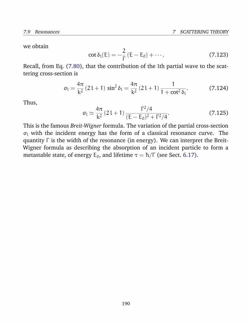
7.9 Resonances 7 SCATTERING THEORY
we obtain
cot δl(E) = −2
Γ(E− E0) + · · · . (7.123)
Recall, from Eq. (7.80), that the contribution of the lth partial wave to the scat-
tering cross-section is
σl =4π
k2(2 l+ 1) sin2 δl =
4π
k2(2 l+ 1)
1
1+ cot2 δl. (7.124)
Thus,
σl '4π
k2(2 l+ 1)
Γ 2/4
(E− E0)2 + Γ 2/4. (7.125)
This is the famous Breit-Wigner formula. The variation of the partial cross-section
σl with the incident energy has the form of a classical resonance curve. The
quantity Γ is the width of the resonance (in energy). We can interpret the Breit-
Wigner formula as describing the absorption of an incident particle to form a
metastable state, of energy E0, and lifetime τ = h/Γ (see Sect. 6.17).
190