Friction and compliance identi cation in a vehicle’s ... · in a vehicle’s steering system (DCT...

Friction and compliance identificationin a vehicle’s steering system

(DCT 2009.059)

M.W.F. Mol (0571229)

.

Coach: Ir. P. v.d. Linden

Supervisor: Prof. Dr. H.Nijmeijer

Technische Universiteit EindhovenDepartment Mechanical EngineeringDynamics and Control Group

Eindhoven, Januari, 2010

Abstract

Vehicle interaction during steering maneuvers has been widely addressed in technical lit-erature. However there is still an area of which there is much to be learned, namely thesteering feel for a driver while performing small steering maneuvers also known as ”on-center” handling. An overtaking maneuver on the highway is good example of ”on-center”handling. Steering behaviour and feel for on-center handling is greatly determined byfrictions and compliances in the steering system and suspension parts. Therefore in thisreport the possibilities are examined for a systematical approach of measuring frictionsand compliances in a vehicle’s steering system while performing on-center manoeuvres.As a first step instrumentation and measurements are made on a vehicle to determinethe feasibility for this identification. The results look promising for extended instrumen-tation and identification. Also a multi-body model is adapted to accurately simulate theon-center manoeuvres. An existing model is extended to contain more complexity of thesteering system and suspension. The possibilities herein and stability for the model areexamined. The measurements from testing can be used to accurately simulate the vehicle’sbehaviour. Optimization tools can be used to further optimize the model for the on-roadmeasurements.

i

Contents

Abstract i

1 Introduction 1

1.1 Test vehicle and multibody model . . . . . . . . . . . . . . . . . . . . . . . 2

1.2 Report outline . . . . . . . . . . . . . . . . . . . . . . . . . . . . . . . . . . 2

2 On-center handling 3

2.1 On-center maneuvers . . . . . . . . . . . . . . . . . . . . . . . . . . . . . . . 3

2.2 Objective parameters . . . . . . . . . . . . . . . . . . . . . . . . . . . . . . . 4

3 Instrumentation analysis 6

3.1 Determination of the steering wheel angle . . . . . . . . . . . . . . . . . . . 6

3.2 Determination of lateral acceleration and yaw rate . . . . . . . . . . . . . . 8

3.3 Determination of steering wheel torque . . . . . . . . . . . . . . . . . . . . . 10

3.4 Other instrumentation . . . . . . . . . . . . . . . . . . . . . . . . . . . . . . 13

4 Measurement results and objective parameters 15

4.1 Conclusions . . . . . . . . . . . . . . . . . . . . . . . . . . . . . . . . . . . . 18

5 Multi-body model 20

5.1 Model setup . . . . . . . . . . . . . . . . . . . . . . . . . . . . . . . . . . . . 20

5.2 Simulation results . . . . . . . . . . . . . . . . . . . . . . . . . . . . . . . . 22

5.3 Optimization . . . . . . . . . . . . . . . . . . . . . . . . . . . . . . . . . . . 25

6 Conclusions and recommendations 26

6.1 Conclusions . . . . . . . . . . . . . . . . . . . . . . . . . . . . . . . . . . . . 26

6.2 Recommendations for future research . . . . . . . . . . . . . . . . . . . . . . 26

A Neon Suspension 28

B Strain gauges 30

C Future model recommendations 33

ii

CONTENTS iii

Bibliography 35

Chapter 1Introduction

Vehicle interaction during steering maneuvers has been widely addressed in technical lit-erature. However there is an area of which there is much to be learned. Namely thesteering feel for a driver while performing small steering maneuvers also known as ”on-center” handling [2]. On-center handling involves small lateral accelerations typically notexceeding 2 m/s2. It is of particulary interest in evaluating the handling and steering feelat the highway, for example when making overtaking maneuvers on the highway. Therealready exist numerous procedures and data for the subjective handling of the driver foron-center handling, however there is a lack of objective studies which can quantify this asan objective steering feel.

Steering behaviour and feel for on-center handling is greatly determined by frictions andcompliances in the steering system and suspension parts. For this reason this study isabout identifying the friction and compliance which are present in different connectionsof the steering system.

A procedure for identification of friction and compliance will have to be developed fortesting a vehicle under natural driving. In this way a better understanding of the steeringsystem and wheel suspension behaviour during on-center handling can be made.

A previous study (Bart van Daal [1]) was made concerning the feasibility of friction andcompliance identification on a vehicle’s steering system for on-center driving. The purposeof this report is to continue on the feasibility aspect of friction and compliance identifica-tion. Research is done to examine proper measurement techniques to acquire in a simpleand yet adequate way the vehicle state. Therefore also some on-road tests have been per-formed to analyze the quality of measurements for some instrumentation (steering wheelangle, lateral acceleration and yaw rate).

Also a full multi-body dynamic model of the vehicle is desired with plugged in the deter-mined frictions and compliances to simulate and predict vehicle behaviour for any desiredon-center maneuver. Friction and compliance characteristics used in the model can beoptimized with specialized software tools to match the experimental behaviour of thevehicle.

This research has been performed in association with LMS International, a company thathas a lot of knowledge and experience in the field of vehicle dynamics tests. Data acquisi-tion hardware and simulation software are developed by LMS and can be acknowledged astop of the market quality. This report is written after a three month period of internshipand therefore by far not able to cover all the desired targets but yet there is more insightof tackling certain challenges and fundamenting the feasibility of this project.

1

CHAPTER 1. INTRODUCTION 2

1.1 Test vehicle and multibody model

As a basis for doing this research a Chrysler Neon vehicle is available for instrumentationand measurements. Also for the simulations on a multibody model, a Chrysler Neon modelis available. Unfortunately it turned out the Chrysler Neon vehicle was not street legalbecause of a registration plate issue for test vehicles. For this reason instrumentation andmeasurements were done on a loan car which was a Renault Laguna Estate. This is thesame vehicle that was used for previous measurements made by Bart van Daal [1]. Alsothe multibody model of the Neon has some shortcomings because it turned out that itwas only a visual representation of the Neon’s exterior without any individual bodies andjoints for the chassis and suspension. Therefore the bodies and joints have been createdfrom other existing models or are builded from scratch which are obviously not exact tothe Neon vehicle.

1.2 Report outline

The contents of this report can be split into two parts.

Part 1, measurements:The first part of this report describes the on-road testing of a vehicle. Firstly, the drivingconditions are addressed in chapter 2. In chapter 3 the instrumentation is worked out forthe measurements that were done. Also some research is done to determine the steering-wheel torque for future measurements. The measurement results are presented in chapter4.

Part 2, simulations:In chapter 5 the multi-body dynamic model is discussed. Beginning with the setup of themodel. After that the simulation results are presented and discussed. This part will beconcluded with recommendations for the future model.

In chapter 6 the conclusions and recommendations for future research are presented.

Chapter 2On-center handling

On-center handling describes the steering feel and precision of a vehicle while straight-line driving at medium or high speeds and large radius cornering resulting in low lateralaccelerations [4]. Specific on-center handling maneuvers exist (see section 2.1) that can beperformed by the test vehicle. From these measurements several objective parameters canbe extracted quantifying the steering behaviour and feel for the driver [3], see section 2.2

2.1 On-center maneuvers

Weave test:The weave test is an open-loop procedure conducted on a test track that follows a straight-line path. The vehicle is driven at a nominally constant longitudinal velocity. The standardtest velocity is 100 km/h. Other longitudinal velocities may be used; they should haveincrements of plus or minus 20 km/h from the standard velocity. The weave test proce-dure requires the steering wheel to be subjected to an oscillatory input. The preferredsteering input waveform is nominally sinusoidal, but other steering input waveforms (e.g.triangular) may be used. The frequency of the steering wheel input shall be around 0.2Hz and the resulting peak lateral acceleration should be as close to 2 m/s2 as possible.Also a more random steering wheel input can be applied with different amplitudes andfrequencies, typically frequencies up to 0.4 Hz and peak lateral accelerations of 3 m/s2.

Straight line driving:Straight line driving is similar to the weave test described above only without a steeringwheel input. The only steering action that is made is to keep the vehicle driving in astraight line. Steering wheel corrections should be made at a very low frequency. Thistest is to examine the steering feedback as a result of induced forces and torques troughthe steering system due to the road input.

Other maneuvers:As the weave test is the most important test for the quantification of handling and deter-mining frictions and compliances there are also some other maneuvers. Other maneuverscan be used for optimization and validation of the model. E.g. a step steer test can bemade where the driver has to generate a steering wheel angle as fast as possible and main-tain this angle for a long enough time for the vehicle to reach a steady state condition.More information can be found in literature [2, 4].

3

CHAPTER 2. ON-CENTER HANDLING 4

2.2 Objective parameters

Many subjective tests exist on the on center handling of a vehicle [2]. In subjective tests atest person who is driving the vehicle will have to rate the the vehicle on specific handlingpoints. For example the steering sensitivity can be rated between very nervous and badlyresponsive by the driver. As this method is very dependent on the driver’s opinion andnot very accurate there is a need for a more accurate and objective rating of the vehiclehandling. Therefore objective parameters are introduced for the indication of the vehiclehandling. For objective parameters no driver’s opinion is used. Only measurement datais analyzed to determine the parameters.

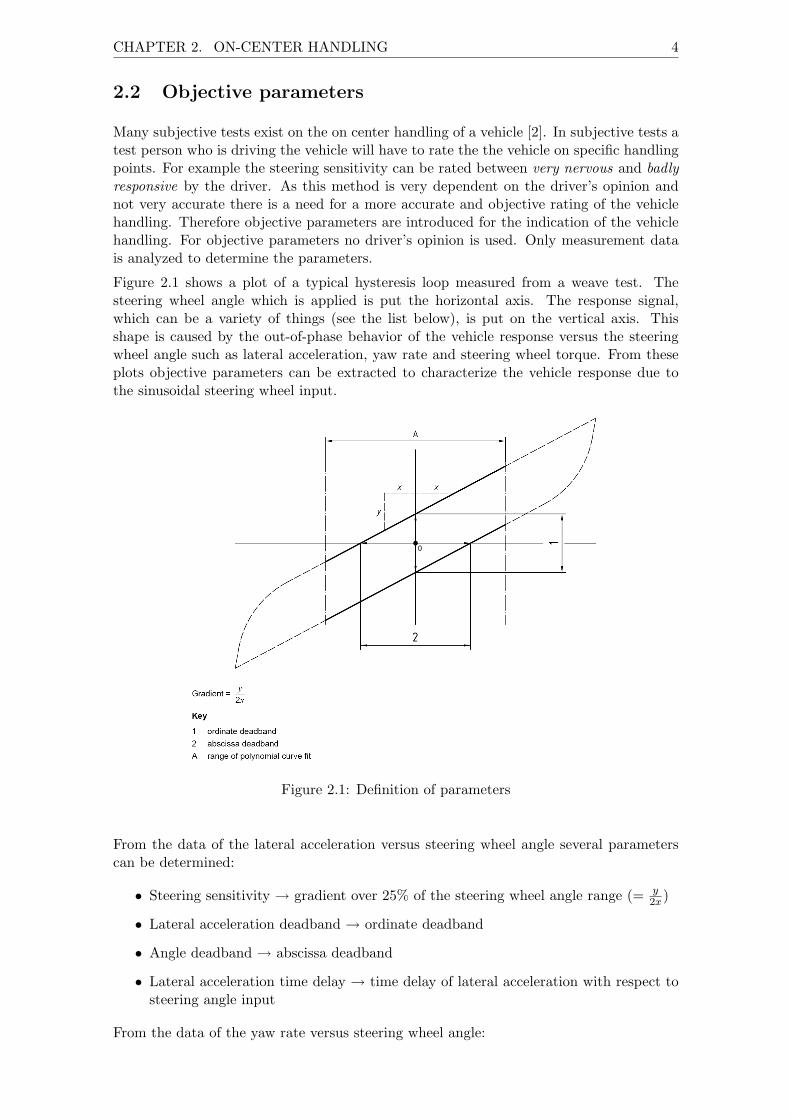
Figure 2.1 shows a plot of a typical hysteresis loop measured from a weave test. Thesteering wheel angle which is applied is put the horizontal axis. The response signal,which can be a variety of things (see the list below), is put on the vertical axis. Thisshape is caused by the out-of-phase behavior of the vehicle response versus the steeringwheel angle such as lateral acceleration, yaw rate and steering wheel torque. From theseplots objective parameters can be extracted to characterize the vehicle response due tothe sinusoidal steering wheel input.

0

Figure 2.1: Definition of parameters

From the data of the lateral acceleration versus steering wheel angle several parameterscan be determined:

• Steering sensitivity → gradient over 25% of the steering wheel angle range (= y2x)

• Lateral acceleration deadband → ordinate deadband

• Angle deadband → abscissa deadband

• Lateral acceleration time delay → time delay of lateral acceleration with respect tosteering angle input

From the data of the yaw rate versus steering wheel angle:

CHAPTER 2. ON-CENTER HANDLING 5

• Yaw rate response gain→ gradient over 25% of the steering wheel angle range (= y2x)

From the data of the steering wheel torque versus steering wheel angle:

• Steering stiffness → average gradient over range x, where x = 10% of peak angle

• Steering friction → ordinate deadband

A full list of parameters can be found in [3].

Chapter 3Instrumentation analysis

Already some instrumentation and measurements has been implemented by Bart vanDaal[1] on a vehicle to investigate a suitable measurement setup for measuring the steer-ing wheel angle and the vehicle’s lateral acceleration and yaw rate.From this information a second measurement is made for the improvement and verificationof these measurement techniques to have a better overview of the measurement quality.Sections 3.1 and 3.2 will describe the setup of the instrumentation that was made. Sec-tion 3.3 will describe a procedure for future instrumentation for the measurements of thesteering wheel torque. Further instrumentation is briefly addressed in section 3.4.

3.1 Determination of the steering wheel angle

The steering wheel angle is measured by means of a draw wire sensor attached to thesteering wheel. The used draw wire displacement sensor is a WDS-750-P60-SR-U man-ufactured by Micro-Epsilon which has a wire length of 750 mm. The sensor housing ismounted on the inside of the front window near the rear view mirror. See figure 3.1.

Figure 3.1: Positioning of the draw wire sensor

6

CHAPTER 3. INSTRUMENTATION ANALYSIS 7

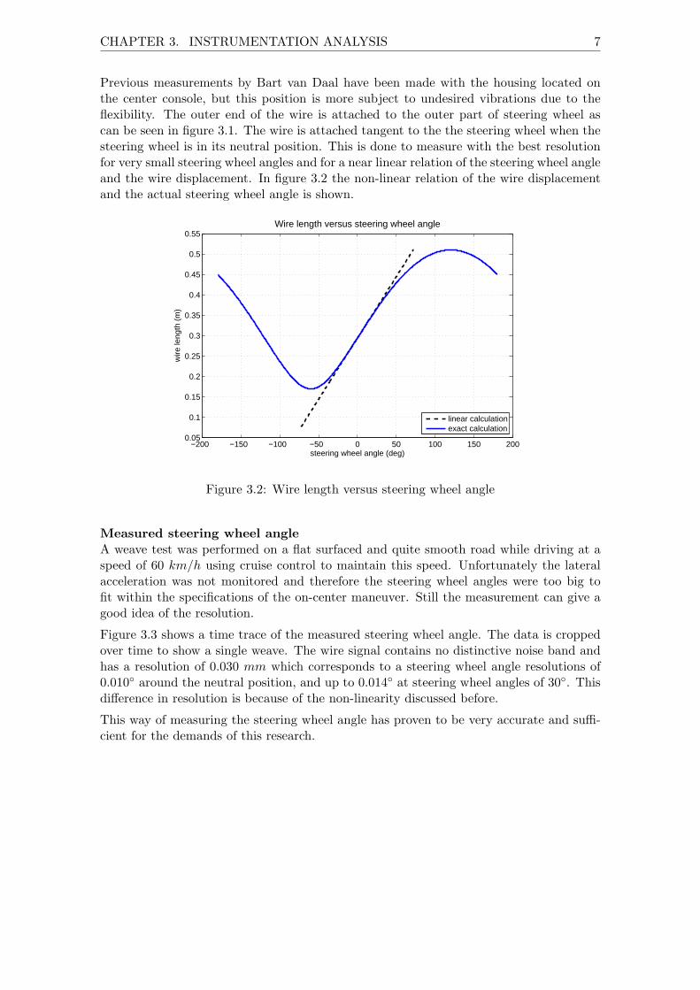
Previous measurements by Bart van Daal have been made with the housing located onthe center console, but this position is more subject to undesired vibrations due to theflexibility. The outer end of the wire is attached to the outer part of steering wheel ascan be seen in figure 3.1. The wire is attached tangent to the the steering wheel when thesteering wheel is in its neutral position. This is done to measure with the best resolutionfor very small steering wheel angles and for a near linear relation of the steering wheel angleand the wire displacement. In figure 3.2 the non-linear relation of the wire displacementand the actual steering wheel angle is shown.

−200 −150 −100 −50 0 50 100 150 2000.05

0.1

0.15

0.2

0.25

0.3

0.35

0.4

0.45

0.5

0.55Wire length versus steering wheel angle

steering wheel angle (deg)

wire

leng

th (

m)

linear calculationexact calculation

Figure 3.2: Wire length versus steering wheel angle

Measured steering wheel angleA weave test was performed on a flat surfaced and quite smooth road while driving at aspeed of 60 km/h using cruise control to maintain this speed. Unfortunately the lateralacceleration was not monitored and therefore the steering wheel angles were too big tofit within the specifications of the on-center maneuver. Still the measurement can give agood idea of the resolution.

Figure 3.3 shows a time trace of the measured steering wheel angle. The data is croppedover time to show a single weave. The wire signal contains no distinctive noise band andhas a resolution of 0.030 mm which corresponds to a steering wheel angle resolutions of0.010◦ around the neutral position, and up to 0.014◦ at steering wheel angles of 30◦. Thisdifference in resolution is because of the non-linearity discussed before.

This way of measuring the steering wheel angle has proven to be very accurate and suffi-cient for the demands of this research.


15 15.5 16 16.5 17 17.5 18 18.5 19 19.5 20−30

−20

−10

0

10

20

30Steering wheel angle (SWA) versus time

time (s)

SW

A (

deg)

linear calculationexact calculation

Figure 3.3: Measured steering wheel angle versus time

3.2 Determination of lateral acceleration and yaw rate

In order to measure the lateral acceleration and yaw rate of the vehicle accelerometers areused. The accelerometers are of a DC type which are able to measure also at very lowfrequencies. This is needed because the steering wheel input will be around 0.2 Hz. Theinstrumentation used is MWS 5401 manufactured by MWS Sensorik. The accelerometersare tri-axial to measure accelerations in all 3 directions. The measuring range is 25 gwhich is more than enough. Lower range accelerometers are desired but not available atthe moment of testing. Typical lateral accelerations should not exceed more than 3m/s2.

Four accelerometers are mounted on the Renault Laguna. Each one in each corner onthe chassis of the car. For lateral acceleration and yaw rate determination two accelerom-eters are sufficient (one in the front and one in the rear). Because of the placement offour accelerometers the lateral acceleration and yaw rate can be determined twice (forvalidation).

ay

vx

Ψ.

ay front left

ay rear left

½L

½L

Figure 3.4: Steering wheel angle versus time


Assuming the accelerometers are positioned to have the same distance to the center ofgravity (1/2L). Lateral acceleration:

ay =ayfront

+ ayrear

2[m/s2] (3.1)

where ayfront=

ayfrontleft+ayfrontright

2

Yaw velocity:

Ψ =vyfront

+ vyrear

2πL· 360[deg/s] (3.2)

Measured lateral accelerationFigure 3.5 shows a time trace of the measured lateral accelerations. The data is croppedto show a single weave. The measured signals from the accelerometers show a lot of noiseas can be seen in figure 3.5. This is because of the strain gauge principle which is usedfor these DC-accelerometers. Lower range accelerometers may reduce the noise amplitudeas they are more sensitive. MATLAB is used to filter out the noise without creating anyphase shift in the signal by means of an idealfilter. The idealfilter is a pass-filter for therange 0 > f ≤ 5Hz. A high sample frequency is desired in order to have a better filteredsignal (more data points to average for an interval). The current sampling frequency usedfor this measurement was 1024 Hz but a higher sampling frequency is desired for betterfiltering.

49 50 51 52−5

−4

−3

−2

−1

0

1

2

3

4

5Lateral accelerations versus time

time (s)

a y (m

/s2 )

front rightfront leftfiltered data

49 50 51 52−5

−4

−3

−2

−1

0

1

2

3

4

5

time (s)

rear rightrear leftfiltered data

Figure 3.5: Measured lateral accelerations versus time

The filtered signals for the left and right side accelerometers are very similar and a dis-tinction is difficult to make from these plots. This indicates that the signals are of a goodquality. Noise is successfully canceled after filtering. In further calculations and analysisfor lateral acceleration and yaw rate both left and right sensor signals are averaged.


3.3 Determination of steering wheel torque

As stated before in this chapter measuring only steering wheel angle, lateral accelerationand yaw rate is not sufficient for this research. An other important signal will be thesteering wheel torque. Torque on the steering is an important factor for the steering feelfor the driver. No measurements have been made yet concerning the steering wheel torquebut an analysis is made to prove the feasibility.

Strain gauges

In order to measure this torque strain gauges can be placed somewhere on the steeringwheel column. It is preferred to place the strain gauges as close to the steering wheel aspossible on the steering wheel column to have a good representation of torque felt by thedriver at the steering wheel. The strain gauges will measure shear strain on the columncaused by the torque acting on the steering wheel column. From the measured strain thetorque can be derived directly because the strain is proportional to the torque acting onthe steering column.

Figure 3.6 shows an overview of how the strain gauges have to be attached to the steeringcolumn. Mt represents the applied torque on the column. The strain gauges are numberedby the numbers 1 - 4.

Figure 3.6: Overview of the positioning of strain gauges for measuring torsional strain

A total of four strain gauges (in a Wheatstone Bridge configuration) is needed for max-imum resolution and sensitivity [6, 7]. Also bending and the influence of temperatureare compensated with a full Wheatstone Bridge setup. Figure 3.7 shows the WheatstoneBridge configuration.

More information on the principle of a Wheatstone bridge configuration for measuringtorque can be found in appendix B.


Figure 3.7: Wheatstone Bridge configuration

Steering wheel column thickness

On-center driving involves relatively low steering wheel torques, estimated to be around 5Nm maximum. For this reason the strain gauges will have to be able to measure very smallstrains. If a steering wheel column is too thick the measurable strains will be too low be-cause of the increasing torsional stiffness for larger column diameters. Therefor a suitabledimension of the axle’s diameter is critical for enough resolution for the measurements.

Calculations have been made to find the actual strain on the surface of a steering columnfor different diameters. To have enough resolution and accuracy on the measurementsthe demand will be that for 5 Nm of torque the measured strain will have to be at least20 microstrain (µε). This is to have enough resolution on the steering wheel torque toaccurately identify frictions in the steering system.

The torsional strain (γ) equals the torsional stress (τ) divided by torsional modulus ofelasticity (G) [6].

γ = 2 · µε@45◦ =τ

G(3.3)

where the torsional strain equals twice the actual measured strain (µε@45◦).

τ = Mtd

2 · J(3.4)

where torsional stress (τ) equals the torque (Mt) multiplied by the radius of the column(d/2), divided by the polar moment of inertia (J).

In figure 3.8 the strain on the surface of a solid steel shaft is plotted versus the diameterof the shaft when it is subjected to 5 Nm of torque.

Parts of the steering wheel column can also be hollow. Figure 3.9 shows the the same asfigure 3.8 but now for hollow shafts with several different wall thicknesses.


15 16 17 18 19 20 21 22 23 24 25 26 27 28 29 30 31 32 33 34 350

5

10

15

20

25

30

35

40

45

Torsional strain on a solid column (steel)

axle diameter (mm)

µε @

45

° (−

)

5 Nm applied torque

Figure 3.8: Strain on a solid steel axle for different diameters

20 21 22 23 24 25 26 27 28 29 30 31 32 33 34 35 36 37 38 39 400

10

20

30

40

50

60Torsional train on a hollow column (steel)

axle outer diameter (mm)

µε @

45

° (−

)

t =1 mmt =2 mmt =3 mmt =4 mm

Figure 3.9: Strain on hollow steel axles for different diameter and wall thickness

The Chrysler Neon

The steering column from a Chrysler Neon vehicle has been examined for torque mea-surements. There is not much space on the axle that is both cylindrical shaped and wellexposed. Figure 3.10 shows the available parts of the steering axle to measure strain.There are two candidate locations for applying strain gauges indicated by the circles infigure 3.10.

- Location 1: This is a solid shaft with a relatively small diameter of 19 mm. The problemis the short available length to apply strain gauges. This may be solved by making somemodifications on the spring mounted on top of it to get more clearance.

- Location 2: This is a hollow shaft of 40 mm in diameter. The wall thickness is unknown


1

2

Figure 3.10: Picture of the steering axle at the foot pedals location

because it is sealed on both sides. It has enough clearance for applying strain gauges. Theproblem however is the large diameter which makes it very stiff resulting in low, hard tomeasure, strain.

The strain on location 1 is calculated to be around 23 microstrain (µε) at 5 Nm of torque.For location 2 the strain for a wall thickness of 2 mm would be around 7 µε. Comparingthe strain on both locations it becomes clear that location 1 is favorable to location 2.

Instrumenting on location 1 should give enough resolution on the torque signal. Althoughit still has to be proven by actual measurements measuring steering wheel torque usingstrain gauges in the way as described here seems feasible.

3.4 Other instrumentation

This study does not yet go into detail of identifying and measuring frictions and compli-ances within specific parts of the steering system and suspension. The vehicle will haveto be more extensively instrumentated to identify all the significant frictions and com-pliances occurring in the steering system and suspension parts. Acquiring these data forfrictions and compliances will give more insight of the vehicle behavior and steering feelfor on-center driving. These objective measurements can be used to quantify and supportcertain vehicle behavior and feel.

For measuring friction the force or torque measurements have to be made before and afterthe location where the friction is present. To measure compliance the measurement ofdisplacement or angle must also be made before and after the location where complianceis present.

Commonly there is only very limited free space for instrumentation. Some frictions andcompliances can not be isolated and measured separately. The compliance from the torsion


bar in the steering column at the steering rack for instance can not be measured directly.A solution will be to measure the angle of the ingoing shaft into the steering rack housingand measuring displacement of the outer ends of the rack. In this way a generalizedcompliance can be determined for all the compliances acting between the two measurementpoints including the torsion bar.

Not only frictions and compliance in the steering system characterize the steering behavior.Also friction and compliance from the suspension parts will have a significant contributionto this. Therefore instrumentation will also have to be made on certain suspension parts.

Chapter 4Measurement results and objectiveparameters

In this chapter the measurement results from the Renault Laguna Estate will be processedand presented. Already some measurement data have been presented in section 3.1 and 3.2to prove the measurement quality. In this chapter the measurement signals are investigatedfurther and available on-center parameters are determined.

As stated before only the steering wheel angle and lateral accelerations have been mea-sured. The measurement techniques can be found in section 3.1 and 3.2. From this limitedset of signals also the vehicle yaw rate is calculated.

Type of test

A weave test is performed on a flat surfaced road at a constant speed of 60 km/h. Asinusoidal steering wheel angle is applied by the driver. The frequency of the steeringwheel angle was kept at approximately 0.2 Hz. The amplitude of the steering wheel anglewas limited by the measured maximum lateral acceleration of the vehicle. Typically themaximum lateral acceleration should be around 0.2 m/s2.

Time signals

Steering wheel angle:

Figure 4.1 shows the steering wheel angle versus time. The measurement data is reducedover the the time axis to show only the performed weaves.

Lateral acceleration:

Figure 4.2 shows the lateral accelerations for the same interval as the steering wheel anglein figure 4.1. The acceleration signals are filtered because the signals contain relativelyhigh levels of noise. The filtered signals are almost identical for the left and right sensors.Therefore the left and right sensor measurements will be averaged. No specific accelera-tions in z-direction, to measure body roll, could be distinguished so these are neglected.

15

CHAPTER 4. MEASUREMENT RESULTS AND OBJECTIVE PARAMETERS 16

35 40 45 50 55 60−40

−30

−20

−10

0

10

20

30

40

50Steering wheel angle versus time

time (s)

SW

A (

deg)

linearexact

Figure 4.1: Steering wheel angle versus time

35 40 45 50 55 60−5

−4

−3

−2

−1

0

1

2

3

4

5

time (s)

a y (m

/s2 )

Lateral acceleration data

front rightfront left

35 40 45 50 55 60−5

−4

−3

−2

−1

0

1

2

3

4

5

time (s)

a y (m

/s2 )

Filtered data

front rightfront left

35 40 45 50 55 60−5

−4

−3

−2

−1

0

1

2

3

4

5

time (s)

a y (m

/s2 )

rear rightrear left

35 40 45 50 55 60−5

−4

−3

−2

−1

0

1

2

3

4

5

time (s)

a y (m

/s2 )

rear rightrear left

Figure 4.2: Lateral acceleration versus time


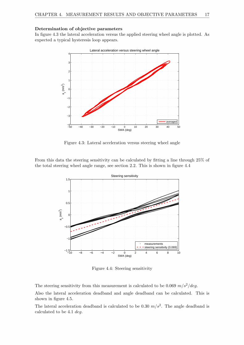
Determination of objective parametersIn figure 4.3 the lateral acceleration versus the applied steering wheel angle is plotted. Asexpected a typical hysteresis loop appears.

−50 −40 −30 −20 −10 0 10 20 30 40 50−4

−3

−2

−1

0

1

2

3

4Lateral acceleration versus steering wheel angle

SWA (deg)

a y (m

/s2 )

averaged

Figure 4.3: Lateral acceleration versus steering wheel angle

From this data the steering sensitivity can be calculated by fitting a line through 25% ofthe total steering wheel angle range, see section 2.2. This is shown in figure 4.4

−10 −8 −6 −4 −2 0 2 4 6 8 10−1.5

−1

−0.5

0

0.5

1

1.5Steering sensitivity

SWA (deg)

a y (m

/s2 )

measurementssteering sensitivity (0.069)

Figure 4.4: Steering sensitivity

The steering sensitivity from this measurement is calculated to be 0.069 m/s2/deg.

Also the lateral acceleration deadband and angle deadband can be calculated. This isshown in figure 4.5.

The lateral acceleration deadband is calculated to be 0.30 m/s2. The angle deadband iscalculated to be 4.1 deg.


−6 −4 −2 0 2 4 6

−0.5

−0.4

−0.3

−0.2

−0.1

0

0.1

0.2

0.3

0.4

0.5

Deadbands

SWA (deg)

a y (m

/s2 )

angle deadband (4.1 deg)

lateral acceleration deadband (0.30 m/s2)

Figure 4.5: Lateral acceleration & angle deadbands

In figure 4.6 the yaw rate versus the steering wheel angle is plotted. As expected also herea typical hysteresis loop appears.

−50 −40 −30 −20 −10 0 10 20 30 40 50−10

−8

−6

−4

−2

0

2

4

6

8

10Yaw rate versus steering wheel angle

SWA (deg)

yaw

rat

e (d

eg/s

)

Figure 4.6: Yaw rate versus steering wheel angle

From this data the yaw rate response gain can be calculated by fitting a line through 25%of the steering wheel angle range, see section 2.2.

Figure 4.7 shows the yaw rate response gain.

The yaw rate response gain is calculated to be 0.21 deg/s/deg.

4.1 Conclusions

The steering wheel angle measurements looks very accurate although some additionalverification measurements will have to be done. Adding an accelerometer to the steering


−10 −8 −6 −4 −2 0 2 4 6 8 10−4

−3

−2

−1

0

1

2

3

4Yaw rate response gain

SWA (deg)

yaw

rat

e (d

eg/s

)

measurementsyaw rate response gain (0.21)

Figure 4.7: Yaw rate response gain

wheel where the wire is attached can be used to verify the steering wheel angle. Theaccelerometer signal will have to be differentiated twice to obtain a position signal. Thissignal can be compared to the draw wire sensor signal for validation.

The lateral acceleration signals shows a lot of noise. Part of this noise is generated bythe accelerometers itself because they are of a DC-type which contains strain gauges.An other part of the noise is generated by the vibrations on the chassis caused by theengine, exhaust, road surface etcetera. Filtering the acceleration signal results in muchsmoother signal. When comparing the left and the right acceleration signal after filteringthey show a very much identical acceleration. The down side of applying this filter is thathigh frequent events are filtered out. Some high frequent events such as stick-slip in thesteering system will not be noticeable after filtering. For deadbands, steering sensitivityand yaw rate response gain determination it proves to be good enough.

Chapter 5Multi-body model

A first version of a full vehicle multi-body model in Virtual.Lab Motion has been developedby Bart van Daal [1]. It was a model of a Chrysler Neon containing a outer body andinterior representation of the Neon. Unfortunately the suspension and steering systemparts were modeled by means of other standard suspension models and the completerear suspension was developed by means of approximating from photographs. Gettinga more exact representation of all the suspension part locations (hard-points) and bodycharacteristics, such as inertias, is too time consuming and will not fit within the timetableof this study. This lack of an exact representation of the multi-body model is a drawbackfor doing measurement on the same physical vehicle and validation between both simulatedand experimental results. In this case it was not possible to do measurements on a ChryslerNeon, so a comparison and validation was already not an option. The model however isstill a good starting point for determining the feasibility of implementing friction andcompliance elements into the model.

In this study the goal is to expand the model’s complexity by adding frictions and compli-ance into the steering system and suspension as well as a better tyre model which is nowavailable. A better overview of the possibilities and stability of this increasingly complexmodel will be governed.

5.1 Model setup

The model provided in [1] was a purely kinematic model with all parts rigid and infinitelystiff joints. One exception for this is the simple tyre model which contains vertical andlateral stiffness. Simulation results for simulating specific on-center manoeuvres were notaccurate and representative for the physical behaviour. To make the model more realisticto the real on-road behaviour of the vehicle the model was expanded.

BushingsBecause a lot of the vehicle suspension part joints have rubber bushings some flexibilityexists between the wheels and chassis. The first step was to replace a lot of the ideal jointsby flexible bushings.

This was done by extracting bushing characteristics, stiffness and damping, from othervehicle models with similar suspension types and plugging this into the Neon model. Thisis done because there was no information available for the Neon vehicle.

TyresSince the model from [1] was almost two years old and made in a earlier version of theVirtual.Lab Motion software it contained a simple tyre model because the possibilities were

20

CHAPTER 5. MULTI-BODY MODEL 21

limited. This tyre model did not contain much dynamic behaviour which is important forsteering manoeuvres. But with a newer version of the software there is the possibility tomodel tyres with ”TNO Delft-tyre”. This is a much more complex dynamic and accuratemodel for simulating more accurate tyre reaction forces and torques. Implementing theTNO Delft-tyre model in the model is very straightforward. An external data file is neededwhich contains tyre characteristics for a specific tyre. As there were not much tyre datafiles available a standard R15 tyre data file is used for the model which is not exactly thesame as the tyres on a Neon but it is quite similar.

Compliance elementsCommonly the most compliance in the steering system is a result of the torsion bar whichcontrols the hydraulic power steering [12]. Therefore a torsion flexible bar is created atthe end of the steering column where it enters the steering rack, called the the pinion. Thetorsion flexibility is created by means of two rigid columns with in-between a torsionalspring. The stiffness of the torsion bar of the Neon was unknown and therefore a stiffnessof another vehicle was used which is representable for a Neon. The data used for thestiffness of this torsion bar is from measurements on a Fiat Punto [12].

This can be seen in figure 5.1.

−5 −4 −3 −2 −1 0 1 2 3 4 5−20

−15

−10

−5

0

5

10

15

20Torsional stiffness data of a torsion bar

torsion bar angle (deg)

torq

ue (

Nm

)

Figure 5.1: Torsion bar characteristic

Friction elementsThe effects of adding multiple fiction elements to the model is examined by means of addingfriction to the steering rack and steering column. Between these two friction locations isthe torsion bar so therefore the friction elements have to be modeled separately. Thesteering rack contains a significant amount of friction. In the paper [12] this friction ismeasured and these values are used to plug into the model. Also the steering columncontains friction due to the bearings and joints at the column. This friction is a lot lowerthan the friction in the steering rack.

Adding frictions into the steering system is not a very straightforward procedure. Thefriction model is kept very simple as the modeling of a more complex friction model isquite difficult in Virtual.Lab Motion. A simple friction function is made as a function ofthe relative velocity between two bodies.

Figure 5.2 shows the friction curve for the steering rack. A hyperbolic tangent function isused to maintain a continuous function for the stability of the calculations. The parametersare chosen is such a way that the transition of the friction value is as small as possible tomaintain a good stability of the calculations.


−1 −0.8 −0.6 −0.4 −0.2 0 0.2 0.4 0.6 0.8 1

x 10−5

−1

−0.5

0

0.5

1

Friction model: tanh(vrel

*106)

func

tion

valu

e (−

)

relative speed (m/s)

Figure 5.2: Friction model

Power steeringHydraulic power steering is very common in passenger cars. To have a good idea of thesteering wheel torque felt by the driver a power steering has to included in the model. Thehydraulic power assist force is in fact a complex function dependent on the torsion barcompliance, hydraulic viscosity, engine RPM, etc. A very simple power steering system ismodeled in Virtual.Lab Motion. A force proportional to the relative angle in the torsionbar is applied to the rack to assist the steering.

5.2 Simulation results

A weave test is performed for a cruising speed of 40 km/h. A sinusoidal steering wheelinput is applied to the steering wheel to have a peak lateral acceleration of around 2m/s2.

The lateral acceleration and yaw rate versus the steering wheel angle shows typical hys-teresis loops; this was not yet the case in the previous model which showed no hysteresis.This is shown in figure 5.3 and 5.4.

−60 −40 −20 0 20 40 60−2.5

−2

−1.5

−1

−0.5

0

0.5

1

1.5

2

2.5Lateral acceleration versus steering wheel angle

SWA (deg)

a y (m

/s2 )

Figure 5.3: Simulated lateral acceleration versus time


−60 −40 −20 0 20 40 60−2

−1.5

−1

−0.5

0

0.5

1

1.5

2Yaw rate versus steering wheel angle

SWA (deg)

Yaw

rat

e (d

eg/s

)

Figure 5.4: Simulated yaw rate versus time

The measurements from the test vehicle discussed in chapter 4 also show these hysteresisloops. This shows that the new simulation model is behaving better towards the realbehaviour of a vehicle compared to the old model which had no hysteresis loops.

From the simulation results also the steering wheel torque can be determined. The steer-ing wheel torque can give more information on the friction and steering feel for the driver.Figure 5.5 shows the steering wheel torque versus time. It can be clearly seen that the fric-

0 2 4 6 8 10 12 14 16 18 20 22−5

0

5Steering wheel torque versus time

time (s)

stee

ring

whe

el to

rque

(N

m)

Model with frictionsModel without frictions

Figure 5.5: Steering wheel torque versus time (simulation)

tions in the model has quite some influence on the steering wheel torque. The magnitudeof the frictions that were used are from measurement on a Fiat Punto [12]. The frictionvalues are 184.7 N and 0.03 Nm for the steering rack and steering column respectively.

Plotting the steering wheel torque against the steering wheel angle, it becomes clear thatthe torque is shifted upwards or downwards depending on the velocity direction of thesteering wheel. See figure 5.6.

The two frictions can be identified when zoomed in at the peak steering wheel angle. Herelock-up is occurring because of the change of velocity direction of the steering wheel. Thesmall vertical part is a result of the steer column friction. The part where there is aconstant slope is caused by the friction inside the steering rack. The reason for this slopeis because of the torsion bar located between the steering wheel and the rack. For a smallangle of the steering wheel the rack can still be locked-up because of the friction being


−60 −40 −20 0 20 40 60−5

0

5Steering wheel torque versus steering wheel angle


stee

ring

whe

el to

rque

(N

m)


Figure 5.6: Steering wheel torque versus steering wheel angle (simulation)

48.8 49 49.2 49.4 49.6 49.8 50 50.2 50.4 50.6

3.6

3.8

4

4.2

4.4

4.6

4.8

Steering wheel torque versus steering wheel angle


stee

ring

whe

el to

rque

(N

m)


Figure 5.7: Zoomed in steering wheel torque versus steering wheel angle (simulation)

greater than the force applied. The slope can be interpreted as the torsional stiffness of thesteer column. In this case the torsional stiffness is solely the torsion bar stiffness becauseall other steering parts are modeled rigid.

So far all the results look promising. Unfortunately there were some unexpected resultsof the forces and torques while doing simulations at higher speeds. Figure 5.8 showsa plot of the steering wheel torque versus the steering wheel angle while simulating aweave test at 100 km/h. Here the loop is going in counter-clockwise direction instead ofclockwise as we saw in figure 5.6 at 40 km/h. This behaviour is assumed to be wrongand does not represent the torque in reality. Despite attempts to identify this problem,the cause of this behaviour is still not very clear. Numerous things can cause the modelto be inaccurate. Namely the suspension connections were not modeled exactly, also theinertias are unknown and guessed, stiffnesses were approximated, etc. Probably deriving amore exact model of the vehicle will not have this undesired behaviour and can give muchmore realistic results. Recommendations for a future model can be found in appendix C.


−10 −8 −6 −4 −2 0 2 4 6 8 10−5

0

5Steering wheel torque versus steering wheel angle


stee

ring

whe

el to

rque

(N

m)

V = 100 km/h

Figure 5.8: Steering wheel torque versus steering wheel angle (simulation for 100 km/h)

5.3 Optimization

To have a more accurate model that responds in the same way as the physical vehicle,the model parameters for the frictions and compliances will have to be fine-tuned. Opti-mization software is available to optimize the model parameters from measurements. Theoptimization software does simulations and compare the results to the actual measure-ments. This is an iterative process in which the optimization software will change modelparameters to have the simulation results converge to the measurement results until theoptimization targets are met within a specified range of tolerance.

Chapter 6Conclusions and recommendations

6.1 Conclusions

MeasurementsThe measurements that were already performed in [1] looked promising but it was notyet very clear if the quality of measurements were sufficient. Therefore the measurementswere reproduced for further analysis. The measurements on the steering wheel angleby means of a draw wire sensor gave very good results. Also the measurements on thelateral acceleration and yaw rate with DC-accelerometers show sufficient quality that wasdemanded. Therefore these measurement techniques can be used for the future of thisproject. This measurement data can give proper results for the dynamic behaviour of thevehicle for on-center driving and can be used for model validation.

Future instrumentationThe frictions and compliances can not be identified by means of this limited amountinstrumentation. For this reason much more instrumentation will have to be done forthe identification of frictions and compliances in a vehicle’s steering system. As for themeasurement of the steering wheel torque, strain gauges can be used. A set of four straingauges can be applied on the steer column to measure the torsional strain. The steeringwheel torque can be derived by means of the proportional relation between the torsionalstrain and torque. The steering wheel torque remains relatively small during on-centermanoeuvres but by finding a suitable location on the column to apply the strain gaugesenough resolution should be governed for the identification of friction.

Multi-body modelThe existing multi-body model has been successfully extended by means of adding bush-ings, compliance, frictions, power steering and a more complex tyre model. The modelcalculations remain stable and the simulation times are very acceptable, typically around3 minutes for a full weave test. Simulation results are promising for a better future com-parison and validation from actual measurements.Simulation results for manoeuvres at high speeds (> 50 km/h) has given unexpected re-sults for the steering wheel torque. This is probably caused by a modeling error or thelack of accuracy of the suspension in the model which has not been solved yet.

6.2 Recommendations for future research

The measurement technique for the steering wheel torque by means of strain gauges hasnot been tested yet. Therefore it is recommended to do more investigation by means of

26

CHAPTER 6. CONCLUSIONS AND RECOMMENDATIONS 27

test measurements for the validation of the measured torque at the steer column.

More research has to be done on further instrumentation of the test vehicle for the iden-tification of friction and compliance in the steering system. It is of particular interestto measure all the significant friction and compliance elements throughout the completesteering system and suspension for small steering maneuvers which all effect the handlingsteering feel for the driver. Not all friction and compliance elements can be measuredseparately. In this case measurements will have to be done including multiple frictionand/or compliance elements.

A more accurate multi-body model of the steering system, suspension parts and inertiasis desired to have representative simulation results. The models that have been imple-mented for friction, compliance and power steering are until now very simple but gavesome improving and promising results. More accurate simulation results are desired andtherefore these models will have to be made more complex while maintaining the stabilityand simulation time limits. As Virtual.Lab Motion is limited in the possibility to modelmore complexity in the steering system a second software package can be used calledAMESim. This software, which is also developed by LMS, is much more powerful in doing1-dimensional calculations and therefore a good alternative. The AMESim model can beplugged in to the Virtual.Lab Motion model to have one complete model for performingmore accurate simulations.

Eventually the simulation results will be compared to the on-road test measurements ofthe same vehicle that is modeled. Optimization tools can then be used to optimize thesimulation model to have a representative virtual model of the vehicle.

Appendix ANeon Suspension

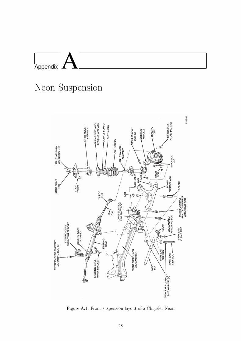
Figure A.1: Front suspension layout of a Chrysler Neon

28

APPENDIX A. NEON SUSPENSION 29

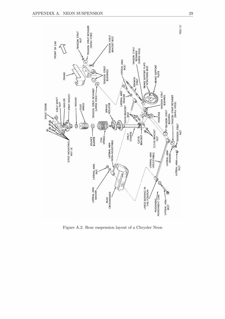
Figure A.2: Rear suspension layout of a Chrysler Neon

Appendix BStrain gauges

Strain is defined as the ratio of the change in length to the initial unstressed referencelength. A strain gage is the element that senses this change and converts it into anelectrical signal. This can be accomplished because a strain gage changes resistance asit is stretched, or compressed, similar to wire. For example, when wire is stretched, itscross-sectional area decreases; therefore, its resistance increases.

The total strain is represented by a change in VOUT . If each gage had the same positivestrain, the total would be zero and VOUT would remain unchanged. Bending, axial, andshear strain are the most common types of strain measured. The actual arrangement ofyour strain gages will determine the type of strain you can measure and the output voltagechange. See Figures C through F.

30

APPENDIX B. STRAIN GAUGES 31

Torsional strain equals torsional stress (τ) divided by torsional modulus of elasticity (G).See Figure F.

γ = 2 · ε @45◦ = τ/G

τ = Mt · (d/2)/J

where torsional stress (τ) equals torque (Mt) multiplied by the distance from the centerof the section to the outer fiber (d/2), divided by (J), the polar moment of inertia. Thepolar moment of inertia is a function of the crosssectional area. For solid circular shaftsonly, J = p(d)π. Strain gages can be used to determine torsional moments as shown inthe equation below. This represents the principle behind every torque sensor.

Mt = τ · (J) · (2/d)Mt = γG · (J) · (2/d)Mt = γG · (pdπ)

Ø = Mt · L/G · (J)

APPENDIX B. STRAIN GAUGES 32

The following table shows how bridge configuration affects output, temperature compen-sation, and compensation of superimposed strains. This table was created using a gagefactor of 2.0, Poissons Ratio of 0.3, and it disregards the lead wire resistance. This chartis quite useful in determining the meter sensitivity required to read strain values. Tem-perature compensation is achieved in many of the above configurations. Temperaturecompensation means that the gages thermal expansion coefficient does not have to matchthe specimens thermal expansion coefficient. Quarter bridges can have temperature com-pensation if a dummy gage is used. A dummy gage is a strain gage used in place of a fixedresistor. Temperature compensation is achieved when this dummy gage is mounted on apiece of material similar to the specimen which undergoes the same temperature changesas does the specimen, but which is not exposed to the same strain. Strain temperaturecompensation is not the same as load (stress) temperature compensation, because Young’sModulus of Elasticity varies with temperature.

Note: Shear and torsional strain = 2 · ε @45◦

Appendix CFuture model recommendations

The model with the extensions described in section 5.1 shows improvements on the vehicledynamic behaviour for on-center simulations. Still a lot of improvement has to be madeon the model.

As stated before the model is not built from actual data for the Chrysler Neon. Governinga model with a much more exact representation of a vehicle can give more accurate andrealistic results.

Also the friction and compliance models are very limited. The friction is for now onlymodeled at just two locations, namely the steer column and rack. More friction locationswill have to be determined and added to the model. Moreover the friction models arevery simple and will have to be made more complex, like adding viscous effects. Espe-cially the steering rack has got a complex friction characteristic because of the hydraulics.Compliances will also have to be extended for other parts in the steering and suspensionsystem.

A viable option is to model certain parts of the steering system in AMESim. AMESimis an other software package by LMS which is powerful in making more complex, usually1-D, calculation to all sorts of systems. The advantage is that for instance the hydraulicpower steering can be modeled more accurately by AMESim. In addition more accurateand complex friction models can be modeled. This AMESim model can than be pluggedinto the Virtual.Lab Motion model to do a complete simulation at once. Figure C.1 showsa model of a hydraulic power steer model.

33

APPENDIX C. FUTURE MODEL RECOMMENDATIONS 34

Figure C.1: Model of a hydraulic power steering system of a vehicle [11]

Bibliography

[1] B. van Daal, ”Friction and compliance identification in a vehicle’s steeringsystem”, DCT Report 2007.095, 2007

[2] K.D. Norman, ”Objective Evaluation of On-Center Handling Perfor-mance”, SAE 840069, 1984

[3] ISO 2003, ”Road Vehicles - Test method for the quantification of on-centrehandling - Part 1: Weave test”, ISO 13674-1, 2003

[4] D.G. Farrer, ”An Objective Measurement Technique for the Quantifica-tion of On-Centre Handling Quality”, SAE 930827, 1993

[5] J.P. Chrstos, P.A. Grygier, ”Experimental Testing of a 1994 Ford Taurusfor NADSdyna Validation”, SAE 970563, 1997

[6] Omega Engineering Inc, ”Positioning strain gages to monitor bending,axial, shear, and torsional loads”, 1999

[7] N. Gittins, ”Short Guide to Strain Gauging Methods”, HBM, 2009

[8] H.B. Pacejka, ”Tyre and vehicle dynamics”, Butterworth-Heinemann,2006

[9] LMS International, ”LMS Virtual.Lab Motion training Basic and Ad-vanced”, LMS, 2009

[10] S. Data, M. Pesce and L. Reccia, ”Identification of steering system param-eters by experimental measurements processing”, D05403 IMechE, 2004

[11] E Viennet, Modelisation de Directions Assistes Hydrauliques, ImagineS.A. FR06882C, 2007

[12] P. Diglio, ”A Test-based Identification Procedure of Rack-rack Case ModelParameters for CAE Ride-comfort simulation”, LMS Italiana, 2009

35

Friction and compliance identi cation in a vehicle’s ... · in a vehicle’s steering system (DCT...

Documents

Transcript of Friction and compliance identi cation in a vehicle’s ... · in a vehicle’s steering system (DCT...