CLASS I FY DEADLY TORNADOS

MirandaHenderson&KatieRubenMat443–Fall2016

ABSTRACT

In order to analyze the occurrence of injuries or fatalities in this dataset, we will have to create a label. This label is formed from looking at two columns provided in the raw dataset for fatalities and injuries. We will create a label column by designating a value of one to tornado occurrences that caused death or injury and a zero otherwise. The next step would be to clean the data. This dataset has no missing values; however, we will want to make sure that the features provided will be beneficial to the classification problem. A crucial aspect of this investigation is to identify features which have multicollinearity. Removing these features will allow these classification methods to work properly. we will perform feature selection and come up with several sets of features to try out on various classification models. It will be important to also determine the existence of outliers and high leverage points. Several models that we will use are KNN, LDA, QDA, logistic regression, multiple linear regression, random forest, SVM, and neural network. In order to determine the best model, we will rely on looking at the ROC plots for each as well as calculating the AUC, sensitivity, accuracy, and MSE. It is important to have a high sensitivity rate. We will also research other machine learning techniques and methods to help predict the number of fatalities or injuries caused by tornadoes.

INTRODUCTION

Tornados are an important aspect of living in certain areas of the country. They can cause death, injury, property damage, and also high anxiety for those who choose to live in areas prone to tornados. Meteorologists are interested in improving their understanding of the causes of tornados as well as when they are to occur and their severity. Here, we look at the number of annual tornados that have occurred in Illinois since 1950. The data used during this simulation comes from the National Oceanic and Atmospheric Administration [2]. The original dataset contains tornados from 1950 to 2015 for every state in the United States. We restrict the data to include only Illinois and its boundary states; this condenses our new dataset to contain 9582 observations. In particular, the goal of this investigation is to predict if a tornado will cause death and injury to humans or not based on characteristics of past tornadic behavior.

As stated by the NOAA [1], “a tornado is a violently rotating column of air, suspended from a cumuliform cloud or underneath a cumuliform cloud, and often visible as a funnel cloud.” In addition, for this violently rotating column of air to be considered a tornado, the column must make contact with the ground. When forecasting tornados, meteorologist’s look for four ingredients in predicting such severe weather. These ingredients are when the “temperature and wind flow patterns in the atmosphere cause enough moisture, instability, lift, and wind shear for a tornadic thunderstorm to occur [1].”

In order to have a better understanding of the data, it is important to note that the features being considered consist of the 18 following descriptions; month of occurrence, F-scale rating, property loss amount, crop loss, start latitude and longitude, end latitude and longitude, length in miles of the tornado, width in yards of the tornado, number of states affected, if the tornado stays in the state it started in, IL, and the 5 surrounding states (IA, IN, KY, MI, and WI). Here, a tornado that has caused injury or death, is represented as a positive classification, 1. The label for this data set is called fatality and injury. This column was created through several data preparation steps in R, see Appendix A. The data consist of an imbalanced label, where 8159 observations are classified as 0 and 1423 observations are classified as 1.

APPROACHTOANALYSIS

Currently, no analysis on this specific data set has been performed to do classification of human harm. With that being said, we implement several data mining methods to analyze this problem. In addition, we identify outliers and high leverage points during the regression analysis. During our analysis, we find this data set does contain several limitations.

The primary limitation is due to the unbalanced proportions of the classes. When considering the full data set, the positive class only comprises 17% of all observations. This may cause our models to have a very low sensitivity rate at the 5% cut-off value for classes. When performing data analysis on classification problems, it is desirable to have a higher sensitivity rate. In the context of this specific problem, we would rather be more accurate about telling the public if an oncoming tornado will induce harm to humans so that they can take the appropriate coverage and safety. We are less concerned if we tell people to take coverage when not as severe of a tornado is oncoming and most likely will not produce harm to humans. This would result in a lower specificity rate. Being incorrect in predictions that results people to take extra safety measures is not bad; however, being incorrect in predictions that tell people they are not in harms way could be devastating. In any classification problem, there will always be a trade off between sensitivity and specificity.

Another limitation to this data set is the amount of multicollinearity present between the predictors. When performing any kind of classification model, it will be extremely important to remove the variables that are multicollinear. The technique we will use to do this is subset selection using methods of forward, backward and best subset feature selection, with the leaps package in R (see Appendix A). In addition, we will follow up with these suggested subsets of predictors by using variance inflation factor to determine if high multicollinearity still exists. Using this process, we devise 2 subsets of features to use to perform several models of data analysis on. Below is a list of techniques that will be implement in this analysis of classifying harm to human by tornados.

DATAMININGMETHODSIMPLEMENTEDINREPORT

• Regression (Appendix B) o Multiple Regression

§ Ridge § Lasso

• Classification (Appendix C) o General Linear Model o LDA: Linear Discriminant Analysis o QDA: Quadratic Discriminant Analysis o KNN: K – Nearest Neighbors

• Tree Based Methods (Appendix D) o Single Classification Tree o Random Forest o Boosting

§ Bernoulli § Adaboost

• Support Vector Machine (Appendix E) o Kernel

§ Linear § Polynomial § Radial § Sigmoid

• Neural Network (Appendix F)

DATAPREPARATION

The first step to any analysis is to prepare the data. In preparing, any observations with missing in any feature column were identified and removed. In addition, the formatting of each column was appropriately set to either numeric, factor, character or string in R. For this specific data, there is a column labeled state, for which takes on the 6 abbreviations of the states included in this analysis. In order to eliminate having a column of factors in the models, we create an indicator matrix (Figure 1), which correlates these factors to dummy variables accordingly for each individual state. In doing so, this creates a data frame which consists of all numeric columns besides my label which is a factor of 0’s and 1’s.

Figure1:IndicatorMatrixofStates(First5RowsShown)

No further preparation was required for this data set. The resulting structure of the data can be seen in Appendix A . We now consider multicollinearity by performing feature selection to determine appropriate feature subsets to be considered for our models.

Additionally, the condensed dataset that will be used for this analysis consists of 9582 observations. The full data set is split randomly using R in order to create our training and testing data to use during the creation and testing of our models. The training and testing data sets contain 4791 observations each.

MULTICOLLINEARITYANDFEATURESELECTION

The first step taken was to observe the correlation plot of the variables which can be seen in Figure 2. From this matrix, we see high positive and negative correlations by the linearity, shape and color from this plot. The strongest positive correlation is with the F-Scale rating with length and width of the tornado’s path. The strongest negative correlation is with ending latitude and longitude.

The next step taken was to determine a subset of features that were not multicollinear. In doing so, forward, backward and subset feature selection on all features were performed. These results can be seen in the Appendix A. Many subsets could have been chosen, but we only consider two sets of features to test with the models. Subset 0 is the full model with all features, we consider this subset when we perform ridge and lasso regression because lasso will perform its own feature selection. Subset 1 contains 9 features and Subset 2 contains 6 features, which can be seen in Figure 3. Additionally, we see that the multicollinearity seems to be acceptable only for Subset 2 and 3 since the VIF<5 for all features.

Figure2:CorrelationMatrixofFeatures

Figure3:VarianceInflationFactor(m0=full,m1=6features,m2=9features)Subset.0=m0,Subset.1=m1,Subset.2=m2

METHODSOFANALYSIS

We begin our model analysis with regression techniques, specifically OLS, ridge, and lasso regression. We follow up with four classification approaches: logistic regression, linear discriminant analysis, quadratic discriminant analysis, and K-Nearest Neighbor approach. In order to ensure there is no multicollinearity, we restrict ourselves to Subsets 1 and 2 identified above. We then implement random forest, support vector machine, and neural network techniques. In each subsection, we summarize our findings for each technique. All corresponding code can be found in Appendices B, C, D, E, and F accordingly. For each method that requires tuning, 10-fold cross validation was performed. In addition, an R loop was created for each method to determine the cut-off value for prediction probabilities by weighing the significance of sensitivity versus accuracy. The results follow below.

REGRESSION

OrdinaryLeastSquares

We begin with multiple linear regression using ordinary least square (OLS) estimates. These estimates produce a model that has low bias and high variance. In R, we created a linear model such that the posterior probability of the positive class had a cut-off rate of 22% which sends an observation to class 1. In addition, we looked for observations that may be outliers or have high leverage; these results can be seen in Figure 4. Although identified, we choose to leave these observations in our model because they are realistic results of tornados that have happened. The confusion matrix for this model can also be seen in Figure 4.

Ridge

The next method implemented is known as ridge regression, which is similar to OLS regression except now we are introducing a penalty term which is known as the “L2” norm. This penalty term is used to help control the amount of variance in the model. Therefore, ridge regression introduces some bias with the reduction in variance. The interpretability of this model is similar to that of the OLS method.

Ridge regression was performed with all 3 subsets of the data. We normalized our predictors before running these subsets. In order to determine the best lambda value for the penalty term in ridge regression, we use 5-fold cross validation (see Appendix B). Each model has a 12% cut-off which provided us with the best sensitivity rate and also a decent accuracy rate. A comparison summary of these three subsets can be seen in Figure 5. Of these models, ridge regression on Subset 1 performed the best with the highest AUC, accuracy, and sensitivity rate. See Figure 7 for AUC values.

Figure4:OLSModelOutliers/LeveragePoints,Cut-OffRateDetermination,ROC/AUC,ConfusionMatrix

Figure5:RidgeModelConfusionMatrix,ExampleofCut-Offboundarydetermination.

Subset0 Subset1 Subset2

Lasso

The last form of a regression model is lasso regression; this model also includes a penalty term. However, now it is an “L1” penalty which allows for the model to perform feature selection. Again, in comparison to the OLS method, lasso will introduce bias and decrease variance. Since this method produces a sparse model, it is an easier model to interpret in relation to ridge and multiple regression.

Again, we ran 5-fold cross validation to choose lambda, the penalty coefficient. We also normalized each of our subsets features before running our models. We also ran this model on all three subsets and performed the same analysis as above to determine the best cut-off percentage for classifying the predictions. Similarly, lasso has the optimal sensitivity and accuracy rate at 12%. As seen in Figure 6, the lasso method only has performed feature selection on Subset 0. Since it did not do feature selection on the other 2 subsets, we expect this method to perform worse than or equal to ridge because the benefit of lasso is to perform feature selection. As expected, of these three models shown in Figure 5, Subset 1 performed the best in relation to AUC, accuracy, and sensitivity. See Figure 7 for AUC values.

RegressionDiscussion

As seen in the ROC plot in Figure 7, the OLS method performed the worst. However, all of the other methods in relation to AUC as the criterion performed similarly. For this analysis, we are most interested in having a high sensitivity rate. The model with the best sensitivity rate, accuracy rate and AUC value is ridge with Subset 1 (Figure 7). This model is declared to be the best regression model during this analysis. This confirms that the feature selection process of the lasso was not beneficial for this data. All R code corresponding to this regression analysis is seen in Appendix B.

CLASSIFICATION

All classification problems, will be performed on Subsets 1 and 2 only. These models work best when multicollinearity has been removed. All cutoff boundaries for classes were found through the same looping structure discussed for regression, comparing the trade-off between accuracy and sensitivity.

Figure6:LassoModelConfusionMatrix,ExampleofCut-Offboundarydetermination.

Subset0 Subset1 Subset2

Figure7:ComparisonofRegressionModels

LogisticRegression

The first designated classification model that will be used is logistic regression. This model is less flexible than OLS, Ridge, and Lasso which means it will have a lower variance and higher bias. The coefficients of this model are estimated by the maximum likelihood function. This model has the potential to be good because it has no assumptions about the distribution of the data and is also robust to outliers. One thing to note, is that logistic regression works best when we have linear boundaries between classes.

Observing the two models in Figure 8, Subset 1 has the better AUC value and sensitivity rate. The accuracy rate is fairly similar between the models. The class cut-off boundary for these models were both at 12%. This value was discovered by using a loop in R to determine an appropriate trade off between accuracy and sensitivity.

LinearDiscriminantAnalysis

Linear discriminant analysis (LDA) is another classification method which has linear boundaries. This method assumes the same covariance matrix between the classes. In addition, it is a less flexible method resulting in lower variance for a trade off of higher bias. The coefficients of this model are estimated from the Gaussian distribution. One limitation of LDA is that it is not robust to outliers.

When comparing the two LDA models in Figure 9, it is seen that Subset 1 performs better with respect to AUC and accuracy. It has a 2% lower sensitivity rate, but this is not drastic. The class cut-off boundary used for these models were 9% and 8% respectively for Subset 1 and 2.

QuadraticDiscriminantAnalysis

Quadratic discriminant analysis (QDA) is a method which introduces non-linear boundaries between classes in a classification problem. It is known that QDA is more flexible than LDA, hence QDA has high variance and lower bias than LDA. Unlike LDA, QDA assumes different covariance matrices for each class, but the coefficients are from the Gaussian distribution.

When comparing the two QDA models in Figure 10, it is seen that Subset 1 with a cut-off rate of 5% has an extremely low sensitivity rate which is not good. The model for Subset 2 with a cut-off rate of 10% has more acceptable values for AUC, accuracy, and sensitivity than the model for Subset 1 (refer to Figure 10). From this comparison, having more features was not beneficial for model building using this method.

Figure8:LogisticRegression

Subset1 Subset2

Subset1 Subset2

Figure9:LinearDiscriminantAnalysis

K-NearestNeighbors

The final version of a classification method used is K-nearest neighbors (KNN). In this method, we’re interested in demonstrating the effect of normalizing the features versus not. As seen in Figure 11, the normalized data performed better. In addition, the normalized data for both subsets produced the same results for the confusion matrices and ROC plots. This method is a non-parametric method that does not rely on any prior assumptions. KNN has non-linear boundaries and is more flexible than other methods. In order to determine the value of K for the number of nearest neighbors, we performed 10-fold CV using the caret package in R. Figure 11, shows that all of these models perform poorly with respect to accuracy and AUC. Each of these models have a 6% cut-off value to determine the class of the prediction.

ClassificationDiscussion

Based on the four models discussed above, it is clear that this data has linear boundaries. QDA and KNN performed the worst of the considered methods for each subset. The worst model is QDA for Subset 1 which shows us a 56% sensitivity rate even with considering a tradeoff between accuracy and sensitivity as described earlier. As demonstrated in figure 12, we see that both subsets perform similarly for each respective model when comparing AUC, accuracy, and MSE. In addition, the linear decision boundary models have performed best. Of these 10 models, the model to consider using would be GLM or LDA for Subset 1 or 2. In the interest of interpretation of the model, it is always best to choose the model with fewer features. Thus, Subset 2 would be a good choice. All R code associated to the classification methods can be seen in Appendix C.

Figure11:KNNappliedtonormalizedandnon-normalizedSubset1andSubset2.

Subset2Subset1

Figure12:ClassificationMethodComparison

Subset1 Subset2

Figure10:QuadraticDiscriminantAnalysis

TREEBASEDMODELS

All tree based models will be performed using the full number of predictors available, Subset 0. We will investigate the use of a single tree, random forest, and boosting methods. All corresponding R codes is seen in Appendix D.

SingleClassificationTreeMethod

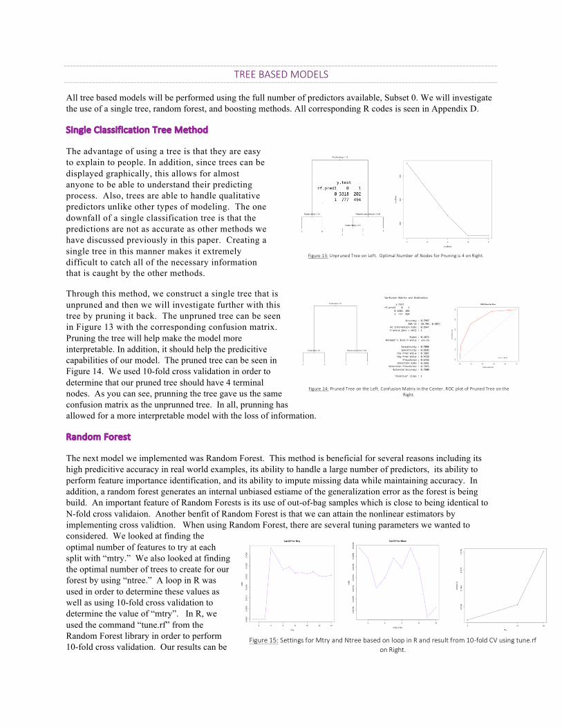
The advantage of using a tree is that they are easy to explain to people. In addition, since trees can be displayed graphically, this allows for almost anyone to be able to understand their predicting process. Also, trees are able to handle qualitative predictors unlike other types of modeling. The one downfall of a single classification tree is that the predictions are not as accurate as other methods we have discussed previously in this paper. Creating a single tree in this manner makes it extremely difficult to catch all of the necessary information that is caught by the other methods.

Through this method, we construct a single tree that is unpruned and then we will investigate further with this tree by pruning it back. The unpruned tree can be seen in Figure 13 with the corresponding confusion matrix. Pruning the tree will help make the model more interpretable. In addition, it should help the predicitive capabilities of our model. The pruned tree can be seen in Figure 14. We used 10-fold cross validation in order to determine that our pruned tree should have 4 terminal nodes. As you can see, prunning the tree gave us the same confusion matrix as the unprunned tree. In all, prunning has allowed for a more interpretable model with the loss of information.

RandomForest

The next model we implemented was Random Forest. This method is beneficial for several reasons including its high predicitive accuracy in real world examples, its ability to handle a large number of predictors, its ability to perform feature importance identification, and its ability to impute missing data while maintaining accuracy. In addition, a random forest generates an internal unbiased estiame of the generalization error as the forest is being build. An important feature of Random Forests is its use of out-of-bag samples which is close to being identical to N-fold cross validaion. Another benfit of Random Forest is that we can attain the nonlinear estimators by implementing cross validtion. When using Random Forest, there are several tuning parameters we wanted to considered. We looked at finding the optimal number of features to try at each split with “mtry.” We also looked at finding the optimal number of trees to create for our forest by using “ntree.” A loop in R was used in order to determine these values as well as using 10-fold cross validation to determine the value of “mtry”. In R, we used the command “tune.rf” from the Random Forest library in order to perform 10-fold cross validation. Our results can be

Figure13:UnprunedTreeonLeft.OptimalNumberofNodesforPruningis4onRight.

Figure14:PrunedTreeontheLeft.ConfusionMatrixintheCenter.ROCplotofPrunedTreeontheRight.

Figure15:SettingsforMtryandNtreebasedonloopinRandresultfrom10-foldCVusingtune.rfonRight.

seen below in Figure 15. We have performed bagging on our random forest when we consider both tuning parameters “mtry” and “ntree.”

Once, we found that the optimal number for “mtry” was 7 features and for “ntree” was 4,500 trees we ran our predictions in R. In doing so, we attained the following feature importance to the right along with the corresponding confusion matrix and ROC plot in Figure 16. The cut off value for our predictions to assign the probabilities to 1 or 0 were found in same manner as discussed during the classification and regression modeling. In this method, the cut off value was at 12%. Refering to the variable importance plot, we see that the F-scale rating, property loss, length, starting and ending latitutdes and longitudes, width, and month are all of significant importance to this model. Therefore, Random Forest has selected to use only 9 features for this model. This selection was made using the Gini index.

BoostedRandomForest:BernoulliDistribution

Here, we implement boosting methods using the Bernoulli distribution. Boosting methods grow trees sequentially by using information from previous trees to grow the proceeding tree. This method essentially learns as it proceeds instead of fitting one large decision tree. By allowing the slow learning, this can improve the performance. Here, we have chosen to create a model with a Bernoulli distribution and with the AdaBoost distribution. Since we have a binary classification problem, we first choose the Bernoulli distribution.

We choose to grow 5000 trees, a shrinkage value of 0.01, and depth of 4. The results from this model can be seen in Figure 17. From the variable importance plot, the F-scale rating and property loss had the largest importance in the model. Additionally, we see that 18 predictors were influential and would be used for the building of this boosting model using a Bernoulli distribution. The summary confusion matrix for the predictions of this model can also be seen in Figure 17. We see from the confusion matrix statistics and ROC plot, this model yielded good results.

BoostedRandomForest:AdaBoostDistribution

In addition to the boosting model in the previous section, we choose to build a boosting model using the AdaBoost distribution. This method produces a sequence of weak classifiers and final predictions are created by a weighted majority vote of the classifiers.

Once again, we choose 5000 trees, a shrinkage value of 0.01, and depth of 4, like for the Bernoulli distribution. The results can be seen below. From the variable importance plot, we see that this model also

Figure17:BernoulliRandomForestStatistics

Figure16:RandomForestStatistics

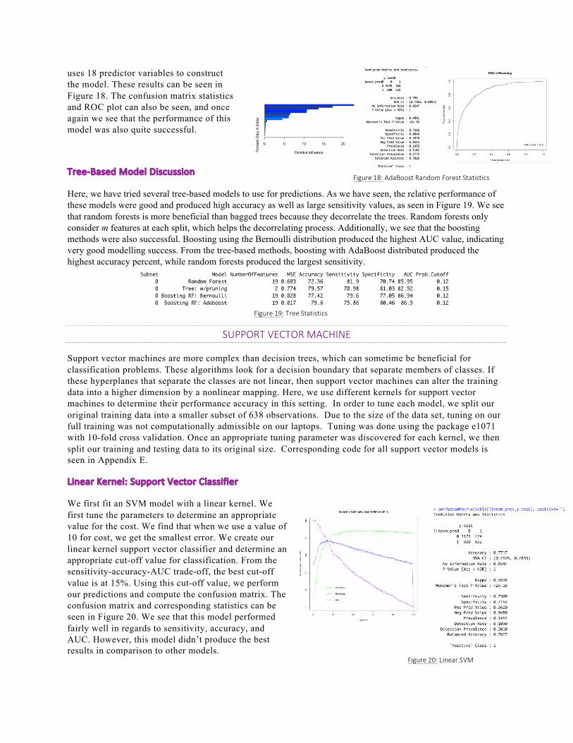
uses 18 predictor variables to construct the model. These results can be seen in Figure 18. The confusion matrix statistics and ROC plot can also be seen, and once again we see that the performance of this model was also quite successful.

Tree-BasedModelDiscussion

Here, we have tried several tree-based models to use for predictions. As we have seen, the relative performance of these models were good and produced high accuracy as well as large sensitivity values, as seen in Figure 19. We see that random forests is more beneficial than bagged trees because they decorrelate the trees. Random forests only consider m features at each split, which helps the decorrelating process. Additionally, we see that the boosting methods were also successful. Boosting using the Bernoulli distribution produced the highest AUC value, indicating very good modelling success. From the tree-based methods, boosting with AdaBoost distributed produced the highest accuracy percent, while random forests produced the largest sensitivity.

SUPPORTVECTORMACHINE

Support vector machines are more complex than decision trees, which can sometime be beneficial for classification problems. These algorithms look for a decision boundary that separate members of classes. If these hyperplanes that separate the classes are not linear, then support vector machines can alter the training data into a higher dimension by a nonlinear mapping. Here, we use different kernels for support vector machines to determine their performance accuracy in this setting. In order to tune each model, we split our original training data into a smaller subset of 638 observations. Due to the size of the data set, tuning on our full training was not computationally admissible on our laptops. Tuning was done using the package e1071 with 10-fold cross validation. Once an appropriate tuning parameter was discovered for each kernel, we then split our training and testing data to its original size. Corresponding code for all support vector models is seen in Appendix E.

LinearKernel:SupportVectorClassifier

We first fit an SVM model with a linear kernel. We first tune the parameters to determine an appropriate value for the cost. We find that when we use a value of 10 for cost, we get the smallest error. We create our linear kernel support vector classifier and determine an appropriate cut-off value for classification. From the sensitivity-accuracy-AUC trade-off, the best cut-off value is at 15%. Using this cut-off value, we perform our predictions and compute the confusion matrix. The confusion matrix and corresponding statistics can be seen in Figure 20. We see that this model performed fairly well in regards to sensitivity, accuracy, and AUC. However, this model didn’t produce the best results in comparison to other models.

Figure19:TreeStatistics

Figure20:LinearSVM

Figure18:AdaBoostRandomForestStatistics

PolynomialKernel:

We now see if a polynomial fit is more appropriate for our data. Once again, we tune the parameters cost, degree, and gamma to determine which will suffice for the model. We find that the error is minimized when cost is 1, degree 3, and gamma is 0.1. Using these parameter values, we create a SVM fit with degree 3. The results from this fitted model are shown in the confusion matrix in Figure 21. We again choose a cut-off value of 0.15 for our predictions. This model has the highest sensitivity rate we have seen thus far. However, it also has the lowest accuracy and specificity rates we have seen through our analysis. This model predicts that almost every tornado to ever occur will be deadly.

RadialKernel:

We extend our SVM models to a radial kernel. Once again, we tune the parameters in order to minimize the error. We determine that when cost is 10 and gamma is 0.1, we minimize the error. Similar to the previous SVM models, we find a cut-off value of 0.15 for this model. The model performance can be seen in Figure 22. We can see from the confusion matrix, that this is model has good specificity and bad sensitivity. The accuracy rate seems to be okay.

SVMDiscussion

In this section, we have created several SVM models with different kernels. In each case, we tuned the parameters in order to determine the most appropriate values that would minimize the errors. The ROC plots for each of these kernels can be seen in Figure 24. We see that the linear SVM performed the best out of all three of the kernels tried. Thus, as seen previously, our data works well with linear assumptions. Additionally, we see from the summary table in Figure 25 that a polynomial assumption produced a model with terrible accuracy in addition to a low AUC value. Considering the cut-off values chosen, it appears that a linear SVM produced the best results for this class of models.

NEURALNETWORKS

The final type of model used in this analysis was a neural network. Neural networks are created from an iterative learning algorithm that is composed of nodes. The input nodes are connected to weighted synapses; a signal flows through the neurons and synapses in order to predict the outcome. Neural networks are able to adapt by changing structure based on the predictive abilities of the training data being passed through the system. This model uses calculated weights as input variables for which these weights are equivalent to the regression parameters of GLM.

Figure21:PolynomialSVM Figure22:RadialSVMFigure24:ROCSVM

Figure25:SVMModelStatistics

All weights are from the standard normal distribution. We used the package “nnet” which allows for only 1 hidden layer. In the future, we may wish to use another package so that we can have multiple hidden layers. Below are the results found.

Using the caret package to perform 10-fold cross validation on our training set, we were able to tune the decay and number of hidden layers’ parameters. The best results occurred when decay was 0.01 and there was a single hidden layer, see Figure 26. An image of our neural network and can be seen in Appendix F along with all corresponding code. We then produced a model using these parameter settings for which we created predictions from. The cut-of value for classifying our predictions we set to 0.88. The ROC with AUC, confusion matrix and cut-off plot can be seen in Figure 27.

RESULTS

Here, we have used multiple methods in order to construct potential models that can be used for predicting whether or not a tornado can be harmful based on several features. We attempt to summarize the results from each of the models that we have constructed in order to compare them and determine which model performed the best.

During this analysis, we looked at many different models in order to determine which would perform the best in terms of predicting harmful tornadoes based on our data. In terms of a model that we classify as successful, it should have large accuracy and sensitivity rates, additionally, it should also have a large AUC value. A comparative chart of our results for each of the constructed models can be seen in Figure 28.

This table organizes the results from highest AUC to lowest. As we can see, the random forest methods performed the best in terms of AUC values. Additionally, these methods produced relatively high accuracy and sensitivity. From this table, we can see that random forest methods are probably the best for the data used here.

In addition, from the table we can see that the next group of highest performing models in terms of AUC are all linear methods: Ridge, GLM, Lasso, and LDA. Thus, we can conclude that either regression or a linear boundary is sufficient for classification for our data.

Figure27:NeuralNetworkStatisticsFigure26:NeuralNetworkTuning

Figure28:ModelStatisticComparison

When comparing AUC values for all of the models considered in this paper, we see that the more complex methods, such as neural networks and SVM methods produced decent results in terms of AUC, as well as, accuracy and sensitivity. However, these more complex methods did not perform as well as random forests in general across all categories.

The K-nearest neighbor performed the worst for this classification problem, producing extremely low AUC values. That is, random guessing would be more sufficient than these methods. Additionally, these methods produced extremely low specificity rates.

Here, we have included the details of all 25 models we constructed and their performance ability are all summarized in Figure 28. We have analyzed these results and determine that high AUC is the best indicator for a better model for these classification problems. In addition to a high AUC, we also must have sufficient accuracy and sensitivity rates in order to consider a model to be good.

DISCUSSION

In this paper, we have used several classification methods in order to predict whether tornadoes will cause injury or fatalities (positive classification). The details of each method and advantages of the chosen methods have been outline within their sections. A summary of the results from all models can be found in Figure 28.

The data used throughout this investigation includes 19 features, subsets of the features were used in those that do not perform feature selection. In order to construct the models used in this project, we used training data to develop the models that were later tested for predictive abilities from test data. A model is determined as sufficient when it produces a large AUC value and high accuracy and sensitivity. Due to the imbalanced nature of the data used, we choose to put more importance on the sensitivity rate rather than the accuracy rate.

Using a loop in R, we construct an accuracy-sensitivity trade-off plot in order to determine an appropriate cut-off value for classification from the predicted probabilities. Using these cut-off values, we could determine the positive classification and construct the ROC plots and confusion matrices.

In this investigation, we used regression methods, classification methods, tree methods, support vector machines, and neural networks in order to predict classes for our data. Regression methods involved preliminary feature selection and subsets of features were tested for each regression method. From Figure 28 in the results section, we see that these regression methods were sufficient for predictions. They usually produced a high AUC value and decent sensitivity and accuracy rates.

The subsets determined from the feature selection used for regression methods were also used for classification methods. The classification methods considered in this paper were logistic regression, LDA, QDA, and KNN classification. From our results section, we can see that the classification methods using linear boundaries were better for AUC and sensitivity. Thus, we can conclude that methods using nonlinear boundaries are not sufficient for this dataset. Additionally, the KNN classifiers performed the worst out of all the models constructed in this investigation in terms of AUC.

From the results seen in the previous section, we determined that the random forests were the best methods in this investigation. We performed random forests with and without boosting methods and all three models produced the top AUC values. Additionally, each model yielded large accuracy and sensitivity values. In terms of our standards for a good model, random forests with boosting using a Bernoulli distribution was the best model. Perhaps, the only downfall of the random forests was the computation time for the large dataset. However, the predictive abilities of these constructed models were very good.

In addition to all of these methods, we used more complex methods like SVM and neural networks. Using the caret package in R, we were able to tune the parameters in order to produce the best model for each of these methods. We found that these models produced good AUC values and the sensitivity accuracy rates typically fell around 75%,

which has been classified as successful in terms of predicting for this unbalanced data in comparison to other models. Although the results for these SVM and neural network models were good and had good predictive abilities, in comparison to simpler methods such as regression or classification methods it may not be worth the computational costs to use such complex models.

Throughout this paper, we have investigated many models for the classification of harmful tornadoes. We have concluded that random forests worked best for the predictive abilities of positive classification. Additionally, we have determined that some of the less computationally sound methods were adequate for good predictions for this data. In the future, an investigation that is more adaptive toward the unbalanced data should be considered in order to improve the classification results seen in this paper. Other improvements for future work on this data set would be to look at transforming variables, considering interaction terms, creating a feature called ZIP code using latitude and longitude provided in the original data set, and perform under-sampling on the predominant class. With more time permitting, we would run more models with a further investigation of these suggested possible improvements.

BIBLIOGRAPHY

[1] Edwards, R. (n.d.). The Online Tornado FAQ. Retrieved March 29, 2016, from http://www.spc.noaa.gov/faq/tornado/

[2] Storm Prediction Center WCM Page. (n.d.). Retrieved March 29, 2016, from http://www.spc.noaa.gov/wcm/#data, Severe Weather Database Files (1950-2015)

[3] James, G., Witten, D., Hastie, T., & Tibshirani, R. (2013). An introduction to statistical learning: With applications in R. New York: Springer.

INDIVIDUALCONTRIBTUIONTOPROJECT

Thisprojectwasequallyworkedonandadvicewassoughtfromeachotherthroughouttheentireprocess.

Katie

• Founddatasetandperformedinitialtesting• PrepareddatainRtobeusedforvariousdataminingmethods• WroteRcode• Compliedresultsintopaper

Miranda

• WroteRcode• Compiledresultsintopaper• Createdpresentation

APPENDIX

A:DATAPREPARATIONCODE

#-------------------#DataPreparation#-------------------my.matrix<-matrix(0,nrow=length(Tornado$State),ncol=length(unique(Tornado$State)))my.matrix[cbind(seq_along(Tornado$State),Tornado$State)]<-1Tornado<-cbind(Tornado,my.matrix)Tornado=Tornado[,-c(2,3,5,6,7,8,12,13)]library(data.table)setnames(Tornado,old=c('1','2','3','4','5','6'),new=c('IA','IL','IN','KY','MI','WI'))Tornado=Tornado[,-3]str(Tornado)sum(is.na(Tornado))Tornado[,c(1,2,3,4,12,13,14)]<-lapply(Tornado[,c(1,2,3,4,12,13,14)],as.numeric)Tornado[,1]<-factor(Tornado[,1])

#------------------------#FeatureSelection#------------------------library(leaps)full.fit.fw<-regSubsets(Injury.Fatality~.,data=Tornado[,1:18],nvmax=17,method="forward")summary(full.fit.fw)par(mfrow=c(2,2))plot(full.fit.fw,scale="Cp",main="ForwardSelection")plot(full.fit.fw,scale="adjr2",main="ForwardSelection")plot(full.fit.fw,scale="bic",main="ForwardSelection")names(coef(full.fit.fw,6))match(c("Fscale.rating","Start.Longitude","Length.Miles","Width.Yards","IA","KY"),names(Tornado))par(mfrow=c(1,1))full.fit.bw<-regSubsets(Injury.Fatality~.,data=Tornado[,1:18],nvmax=17,method="backward")summary(full.fit.bw)par(mfrow=c(2,2))plot(full.fit.bw,scale="Cp",main="BackwardSelection")plot(full.fit.bw,scale="adjr2",main="BackwardSelection")plot(full.fit.bw,scale="bic",main="BackwardSelection")which.min(summary(full.fit.bw)$bic)names(coef(full.fit.bw,6))full.fit.bestSubset<-regSubsets(Injury.Fatality~.,data=Tornado[,1:18],nvmax=17,method="exhaustive")summary(full.fit.bestSubset)plot(full.fit.bestSubset,scale="Cp",main="BestSubset")plot(full.fit.bestSubset,scale="adjr2",main="BestSubset")plot(full.fit.bestSubset,scale="bic",main="BestSubset")which.max(summary(full.fit.bestSubset)$adjr2)names(coef(full.fit.bestSubset,9))match(c("Fscale.rating","Property.Loss.Amount","Start.Longitude","Length.Miles","Width.Yards","Tornado.Stay.in.State","IA","KY","MI"),names(Tornado))

B:REGRESSIONCODE

#-----------------#Splitthedata#-----------------set.seed(16)train=sample(1:nrow(Tornado),nrow(Tornado)/2)test=(-train)x.y.train=Tornado[,1:19][train,]x.train=Tornado[,2:19][train,]y.train=Tornado[,1][train]y.train=as.vector(y.train)x.y.test=Tornado[,1:19][test,]x.test=Tornado[,2:19][test,]y.test=Tornado[,1][test]y=Subset.0$Injury.Fatality#MultipleLinearRegressionOLSMethod

#---------------------------#Multicollinearity#--------------------------library(car)m0<-glm(Injury.Fatality~.,data=x.y.train,family=binomial)vif(m0)#Modelof6predictorsisagreedwithfw,bw,andbestSubsetbasedonBICm1<-glm(Injury.Fatality~Fscale.rating+Start.Longitude+Length.Miles+Width.Yards+IA+KY,data=x.y.train,family=binomial)vif(m1)#UsingAdjr^2ofbestSubsetSelectionm2<-glm(Injury.Fatality~Fscale.rating+Property.Loss.Amount+Start.Longitude+Length.Miles+Width.Yards+Tornado.Stay.in.State+IA+KY+MI,data=x.y.train,family=binomial)vif(m2)#---------------------------------------------------------------#FeatureSubsetstotrywitheachModel.Itincludesthelabel.#---------------------------------------------------------------Subset.0<-Tornado[,]#NofeatureSelectionSubset.1<-Tornado[,c(1,3,4,7,10,11,13,14,17,18)]#Adjr^2bestSubsetSubset.2<-Tornado[,c(1,3,7,10,11,14,17)]#BICbk,fw,andbestSubset

set.seed(16)x.y.train$Injury.Fatality<-as.numeric(x.y.train$Injury.Fatality)-1mod_OLS=lm(Injury.Fatality~.,x.y.train)OLS_pred=predict(mod_OLS,x.test,type="response")#TestingCut-OffValuesOLS.cutoff.sens<-numeric(100)OLS.cutoff.acc<-numeric(100)for(iin1:100){mod_OLS=lm(Injury.Fatality~.,x.y.train)OLS_pred=predict(mod_OLS,x.test,type="response")pred.OLS<-rep(0,length(OLS_pred))pred.OLS[OLS_pred>(i/100)]<-1#table(pred.OLS,y[test])#mean(pred.OLS==y[test])*100OLS.cutoff.acc[i]=mean(pred.OLS==y[test])*100OLS.cutoff.sens[i]=confusionMatrix(table(pred.OLS,(as.numeric(y[test])-1)),positive='1')$byClass[1]}plot(1:100,OLS.cutoff.sens,type="b",xlab="Cutoff%",ylab="Sensitivity/AccuracyRate",main="Subset.0OptimalOLSCutoff%",col="purple")par(new=TRUE)plot(OLS.cutoff.acc,xlab="",ylab="",axes=FALSE,type="b",col="Green")legend(70,60,legend=c(paste("Accuracy"),paste("Sensitivity")),lty=c(1,1),col=c("green","purple"),bty="n")#Usingoptimalcut-offvaluetomakepredictionspred.OLS<-rep(0,length(OLS_pred))pred.OLS[OLS_pred>.22]<-1table(pred.OLS,y[test])mean(pred.OLS==y[test])*100OLS.mse=(mean(pred.OLS-(as.numeric(y[test])-1)^2)*100)confusionMatrix(table(pred.OLS,(as.numeric(y[test])-1)),positive='1')cm.OLS=confusionMatrix(table(pred.OLS,(as.numeric(y[test])-1)),positive='1')cm.OLS$byClass[1]cm.OLS$byClass[2]#ROCplotOLS_pred=predict(mod_OLS,newx=x[test,])roc.OLS.pred=prediction(OLS_pred,(as.numeric(y[test])-1))roc.OLS.perf1=performance(roc.OLS.pred,"tpr","fpr")OLS1=plot(roc.OLS.perf1,main="ROCCurveforOLS",col=2,lwd=2)abline(a=0,b=1,lwd=2,lty=2,col="gray")auc6<-performance(roc.OLS.pred,"auc")auc6<-unlist(slot(auc6,"y.values"))auc6<-signif(auc6,digits=4)*100legend(0.5,0.2,paste(c("AUCOLS="),auc6,sep=""),bty="n")par(mfrow=c(1,1))plot(mod_OLS)Subset.0[c(6401,3264,3339),]#DetectedOutliers

Subset.0[c(8503,9120,7889),]#DetectedHighLeverage#-------------------------#RegressionModelingwithSubset0#-------------------------train=sample(1:nrow(Subset.0),nrow(Subset.0)/2)test=(-train)x=model.matrix(Injury.Fatality~.,data=Subset.0)[,-1]y=Subset.0$Injury.Fatality#LassoRegressionwithall19variables.library(glmnet)set.seed(16)mod_lasso=cv.glmnet(x[train,],y[train],alpha=1,nfold=5,family='binomial')plot(mod_lasso)coef(mod_lasso)lambda_best=mod_lasso$lambda.minlambda_bestlasso.cutoff.sens<-numeric(100)lasso.cutoff.acc<-numeric(100)for(iin1:100){mod_lasso=glmnet(x[train,],y[train],alpha=1,lambda=lambda_best,family='binomial')lasso_pred=predict(mod_lasso,newx=x[test,],s=lambda_best,type="response")pred.lasso<-rep(0,length(lasso_pred))pred.lasso[lasso_pred>(i/100)]<-1#table(pred.lasso,y[test])#mean(pred.lasso==y[test])*100lasso.cutoff.acc[i]=mean(pred.lasso==y[test])*100lasso.cutoff.sens[i]=confusionMatrix(table(pred.lasso,(as.numeric(y[test])-1)),positive='1')$byClass[1]}plot(1:100,lasso.cutoff.sens,type="b",xlab="Cutoff%",ylab="Sensitivity/AccuracyRate",main="Subset.0OptimallassoCutoff%",col="purple")par(new=TRUE)plot(lasso.cutoff.acc,xlab="",ylab="",axes=FALSE,type="b",col="Green")legend(70,60,legend=c(paste("Accuracy"),paste("Sensitivity")),lty=c(1,1),col=c("green","purple"),bty="n")set.seed(16)mod_lasso=glmnet(x[train,],y[train],alpha=1,family='binomial',standardize=TRUE,standardize.response=FALSE,lambda=lambda_best)lasso_pred=predict(mod_lasso,newx=x[test,],type="response")pred.lasso<-rep(0,length(lasso_pred))pred.lasso[lasso_pred>.12]<-1table(pred.lasso,y[test])mean(pred.lasso==y[test])*100lasso.mse=(mean(pred.lasso-(as.numeric(y[test])-1)^2)*100)confusionMatrix(table(pred.lasso,(as.numeric(y[test])-1)),positive='1')cm.lasso=confusionMatrix(table(pred.lasso,(as.numeric(y[test])-1)),positive='1')

cm.lasso$byClass[1]cm.lasso$byClass[2]lasso_pred=predict(mod_lasso,newx=x[test,])roc.lasso.pred=prediction(lasso_pred,(as.numeric(y[test])-1))roc.lasso.perf1=performance(roc.lasso.pred,"tpr","fpr")plot(roc.lasso.perf1,main="ROCSubset.0Lasso",col=2,lwd=2)abline(a=0,b=1,lwd=2,lty=2,col="gray")auc6<-performance(roc.lasso.pred,"auc")auc6<-unlist(slot(auc6,"y.values"))auc6<-signif(auc6,digits=4)*100legend(0.5,0.2,paste(c("AUClasso="),auc6,sep=""),bty="n")#RidgeRegressionwithall19variables.set.seed(16)mod_ridge=cv.glmnet(x[train,],y[train],alpha=0,nfold=5,family='binomial')plot(mod_ridge,main="5-FoldCVRidge(18Features)")coef(mod_ridge)lambda_best=mod_ridge$lambda.minlambda_bestridge.cutoff.sens<-numeric(100)ridge.cutoff.acc<-numeric(100)for(iin1:100){mod_ridge=glmnet(x[train,],y[train],alpha=0,lambda=lambda_best,family='binomial')ridge_pred=predict(mod_ridge,newx=x[test,],s=lambda_best,type="response")pred.ridge<-rep(0,length(ridge_pred))pred.ridge[ridge_pred>(i/100)]<-1#table(pred.ridge,y[test])#mean(pred.ridge==y[test])*100ridge.cutoff.acc[i]=mean(pred.ridge==y[test])*100ridge.cutoff.sens[i]=confusionMatrix(table(pred.ridge,(as.numeric(y[test])-1)),positive='1')$byClass[1]}plot(1:100,ridge.cutoff.sens,type="b",xlab="Cutoff%",ylab="Sensitivity/AccuracyRate",main="OptimalRidgeCutoff%",col="purple")par(new=TRUE)plot(ridge.cutoff.acc,xlab="",ylab="",axes=FALSE,type="b",col="Green")mod_ridge=glmnet(x[train,],y[train],alpha=0,lambda=lambda_best,family='binomial')ridge_pred=predict(mod_ridge,newx=x[test,],s=lambda_best,type="response")pred.ridge<-rep(0,length(ridge_pred))pred.ridge[ridge_pred>.12]<-1table(pred.ridge,y[test])mean(pred.ridge==y[test])*100ridge.mse=(mean(pred.ridge-(as.numeric(y[test])-1))^2)*100confusionMatrix(table(pred.ridge,(as.numeric(y[test])-1)),positive='1')cm.ridge=confusionMatrix(table(pred.ridge,(as.numeric(y[test])-1)),positive='1')cm.ridge$byClass[1]cm.ridge$byClass[2]

ridge_pred=predict(mod_ridge,newx=x[test,],s=lambda_best)roc.ridge.pred=prediction(ridge_pred,(as.numeric(y[test])-1))roc.ridge.perf1=performance(roc.ridge.pred,"tpr","fpr")r0=plot(roc.ridge.perf1,main="ROCSubset.0Ridge",col=2,lwd=2)abline(a=0,b=1,lwd=2,lty=2,col="gray")auc5<-performance(roc.ridge.pred,"auc")auc5<-unlist(slot(auc5,"y.values"))auc5<-signif(auc5,digits=4)*100legend("bottomright",paste(c("AUCridge="),auc5,sep=""),bty="n")#Thesamesetofcodeisusedfortheother2subsets.

C:CLASSIFICATIONCODE

#--------------#Subset.1Classification----->>>>>>->>>>>>>->>>>>>>>>>>---->>>>>>>>>>>#---------------set.seed(16)train=sample(1:nrow(Tornado),nrow(Tornado)/2)test=(-train)x.y.train=Subset.1[,1:10][train,]x.train=Subset.1[,2:10][train,]y.train=Subset.1[,1][train]y.train=as.vector(y.train)x.y.test=Subset.1[,1:10][test,]x.test=Subset.1[,2:10][test,]y.test=Subset.1[,1][test]#------------------------#LogisticRegressionfit#------------------------#Testingmultiplecutoffvalues.glm.cutoff.sens<-numeric(100)glm.cutoff.acc<-numeric(100)for(iin1:100){set.seed(16)glm.fit<-glm(Injury.Fatality~.,data=x.y.train,family=binomial)glm.probs<-predict(glm.fit,x.test,type="response")glm.pred<-rep(0,length(glm.probs))glm.pred[glm.probs>(i/100)]<-1glm.cutoff.acc[i]<-mean(glm.pred==y.test)*100glm.cutoff.sens[i]<-confusionMatrix(table(glm.pred,y.test),positive='1')$byClass[1]}plot(1:100,glm.cutoff.sens,type="b",xlab="Cutoff%",

ylab="Sensitivity/AccuracyRate",main="Subset.1OptimalGLMCutoff%",col="purple")par(new=TRUE)plot(glm.cutoff.acc,xlab="",ylab="",axes=FALSE,type="b",col="Green")legend(70,60,legend=c(paste("Accuracy"),paste("Sensitivity")),lty=c(1,1),col=c("green","purple"),bty="n")#Implementbestcut-offvalueset.seed(16)glm.fit<-glm(Injury.Fatality~.,data=x.y.train,family=binomial)glm.probs<-predict(glm.fit,x.test,type="response")glm.pred<-rep(0,length(glm.probs))glm.pred[glm.probs>.12]<-1table(glm.pred,y.test)mean(glm.pred==y.test)*100glm.mse=(mean(glm.pred-as.numeric(y.test))^2)confusionMatrix(table(glm.pred,y.test),positive='1')cm.glm=confusionMatrix(table(glm.pred,y.test),positive='1')cm.glm$byClass[1]cm.glm$byClass[2]#ROCPlotpred<-prediction(glm.probs,y.test)perfglm1<-performance(pred,"tpr","fpr")plot(perfglm1,main="ROCofLogisticRegressionSubset1")auc<-performance(pred,"auc")auc<-unlist(slot(auc,"y.values"))auc<-signif(auc,digits=4)*100legend("bottomright",paste(c("AUCglm="),auc,sep=""),bty="n")#----------#LDA#---------#Testingmultiplecutoffvalues.lda.cutoff.sens<-numeric(100)lda.cutoff.acc<-numeric(100)for(iin1:100){set.seed(16)lda.fit<-lda(Injury.Fatality~.,data=x.y.train)lda.probs<-predict(lda.fit,x.test,type="response")lda.pred<-rep(0,length(lda.probs$posterior[,2]))lda.pred[lda.probs$posterior[,2]>=(i/100)]<-1lda.cutoff.acc[i]<-mean(lda.pred==y.test)*100lda.cutoff.sens[i]=confusionMatrix(table(lda.pred,y.test),positive='1')$byClass[1]}plot(1:100,lda.cutoff.sens,type="b",xlab="Cutoff%",

ylab="Sensitivity/AccuracyRate",main="Subset.1OptimalLDACutoff%",col="purple")par(new=TRUE)plot(lda.cutoff.acc,xlab="",ylab="",axes=FALSE,type="b",col="Green")legend(70,60,legend=c(paste("Accuracy"),paste("Sensitivity")),lty=c(1,1),col=c("green","purple"),bty="n")set.seed(16)lda.fit<-lda(Injury.Fatality~.,data=x.y.train)lda.probs<-predict(lda.fit,x.test,type="class")lda.pred<-rep(0,length(lda.probs$posterior[,2]))lda.pred[lda.probs$posterior[,2]>=(.09)]<-1table(lda.pred,y.test)mean(lda.pred==y.test)*100lda.mse=(mean(lda.pred-as.numeric(y.test))^2)confusionMatrix(table(lda.pred,y.test),positive='1')cm.lda=confusionMatrix(table(lda.pred,y.test),positive='1')cm.lda$byClass[1]cm.lda$byClass[2]lda.probs<-predict(lda.fit,x.test,type="prob")pred.lda<-prediction(lda.probs$x,y.test)perf.lda<-performance(pred.lda,"tpr","fpr")plot(perf.lda,main="ROCofLDASubset1")auc1<-performance(pred.lda,"auc")auc1<-unlist(slot(auc1,"y.values"))auc1<-signif(auc1,digits=4)*100legend(0.5,0.1,paste(c("AUClda="),auc1,sep=""),bty="n")#-----------#QDA#-----------#SensitivityRateCutoffqda.sens.cutoff<-numeric(100)qda.acc.cutoff<-numeric(100)for(iin1:100){set.seed(16)#browser()qda.fit<-qda(Injury.Fatality~.,data=x.y.train)qda.probs<-predict(qda.fit,x.test,type="response")qda.pred<-rep(0,length(qda.probs$posterior[,2]))qda.pred[qda.probs$posterior[,2]>=(i/100)]<-1qda.acc.cutoff[i]<-mean(qda.pred==y.test)*100qda.sens.cutoff[i]=confusionMatrix(table(qda.pred,y.test),positive='1')$byClass[1]}plot(1:100,qda.sens.cutoff,type="b",xlab="Cutoff%",ylab="Sensitivity/AccuracyRate",main="Subset.1OptimalQDACutoff%",col="purple")

par(new=TRUE)plot(qda.acc.cutoff,xlab="",ylab="",axes=FALSE,type="b",col="Green")legend(70,60,legend=c(paste("Accuracy"),paste("Sensitivity")),lty=c(1,1),col=c("green","purple"),bty="n")set.seed(16)qda.fit<-qda(Injury.Fatality~.,data=x.y.train)qda.probs<-predict(qda.fit,x.test,type="class")qda.pred<-rep(0,length(qda.probs$posterior[,2]))qda.pred[qda.probs$posterior[,2]>=(.05)]<-1table(qda.pred,y.test)mean(qda.pred==y.test)*100qda.mse=(mean(qda.pred-as.numeric(y.test))^2)confusionMatrix(table(qda.pred,y.test),positive='1')cm.qda=confusionMatrix(table(qda.pred,y.test),positive='1')cm.qda$byClass[1]cm.qda$byClass[2]#-ROCplotset.seed(16)qda.fit<-qda(Injury.Fatality~.,data=x.y.train)qda.pred<-predict(qda.fit,x.test,type="prob")pred.qda<-prediction(qda.pred$posterior[,2],y.test)#selecttheprobabilitiesofthepositiveclassperf.qda<-performance(pred.qda,"tpr","fpr")plot(perf.qda,main="ROCQDASubset1")auc2<-performance(pred.qda,"auc")auc2<-unlist(slot(auc2,"y.values"))auc2<-signif(auc2,digits=4)*100legend(0.5,0.2,paste(c("AUCqda="),auc2,sep=""),bty="n")#-------------------#KNN#-------------------set.seed(16)train.X<-as.matrix(x.train)test.X<-as.matrix(x.test)library(caret)ctrl<-trainControl(method="cv",number=10,repeats=3)knnFit<-train(Injury.Fatality~.,data=x.y.train,method="knn",trControl=ctrl,preProcess=c("center","scale"),tuneLength=20)knnFitplot(knnFit,main="KNN:10-FoldCV")#knn.sens.cutoff<-numeric(100)

#knn.acc.cutoff<-numeric(100)#for(iin1:100){#set.seed(16)##knn_pred<-knn(train.X,test.X,y.train,k=28,prob=TRUE)#pred.knn<-rep(0,length(knn_pred))#pred.knn[(attributes(knn_pred)$prob)>=(i/100)]<-1#knn.acc.cutoff[i]=mean(pred.knn==y.test)*100#knn.sens.cutoff[i]=confusionMatrix(table(pred.knn,(as.numeric(y.test)-1)),positive='1')$byClass[1]#}#plot(1:100,knn.sens.cutoff,type="b",xlab="Cutoff%",#ylab="Sensitivity/AccuracyRate",main="Subset.1OptimalKNNCutoff%",col="purple")#par(new=TRUE)#plot(knn.acc.cutoff,xlab="",ylab="",axes=FALSE,type="b",col="Green")#legend(10,30,legend=c(paste("Accuracy"),paste("Sensitivity")),lty=c(1,1),col=c("green","purple"),bty="n")set.seed(16)knn_pred<-knn(train.X,test.X,y.train,k=28,prob=TRUE)pred.knn<-rep(0,length(knn_pred))pred.knn[attributes(knn_pred)$prob>=.6]<-1table(pred.knn,y.test)mean(pred.knn==y.test)*100knn.mse=(mean(pred.knn-(as.numeric(y.test)-1)^2))confusionMatrix(table(pred.knn,(as.numeric(y.test)-1)),positive='1')cm.knn=confusionMatrix(table(pred.knn,(as.numeric(y.test)-1)),positive='1')cm.knn$byClass[1]cm.knn$byClass[2]set.seed(16)knn_pred<-knn(train.X,test.X,y.train,k=41,prob=TRUE)prob<-attr(knn_pred,"prob")pred.knn<-prediction(prob,y.test)perf.knn<-performance(pred.knn,"tpr","fpr")plot(perf.knn,main="ROCKNNnon-standardized")auc3<-performance(pred.knn,"auc")auc3<-unlist(slot(auc3,"y.values"))auc3<-signif(auc3,digits=4)*100legend(0.1,0.9,paste(c("AUCknn="),auc3,sep=""),bty="n")#ScaledfeaturesforKNNlibrary(class)set.seed(16)Normalize<-function(x){return((x-min(x))/(max(x)-min(x)))}norm.x.train<-as.data.frame(lapply(x.train[,1:9],Normalize))

summary(norm.x.train)train.X<-as.matrix(norm.x.train)norm.x.test<-as.data.frame(lapply(x.test[,1:9],Normalize))summary(norm.x.test)test.X<-as.matrix(norm.x.test)set.seed(16)norm.x.y.train<-as.data.frame(lapply(x.y.train[,2:10],Normalize))norm.x.y.train<-cbind(norm.x.y.train,x.y.train$Injury.Fatality)library(caret)ctrl<-trainControl(method="cv",number=10,repeats=3)knnFit<-train(x.y.train$Injury.Fatality~.,data=norm.x.y.train,method="knn",trControl=ctrl,preProcess=c("center","scale"),tuneLength=20)knnFitplot(knnFit,main="KNN:NormalizedData10-FoldCV")library(class)library(caret)set.seed(16)knn_pred.normalized<-knn(train.X,test.X,y.train,k=8,prob=TRUE)pred.knn.normalized<-rep(0,length(knn_pred.normalized))pred.knn.normalized[attributes(knn_pred.normalized)$prob>=.6]<-1table(pred.knn.normalized,y.test)mean(pred.knn.normalized==y.test)*100knn.mse.normalized=(mean(pred.knn.normalized-(as.numeric(y.test)-1)^2))confusionMatrix(table(pred.knn.normalized,(as.numeric(y.test)-1)),positive='1')cm.knn.normalized=confusionMatrix(table(pred.knn.normalized,(as.numeric(y.test)-1)),positive='1')cm.knn.normalized$byClass[1]cm.knn.normalized$byClass[2]knn_pred.normalized<-knn(train.X,test.X,y.train,k=2,prob=TRUE)prob.norm<-attr(knn_pred.normalized,"prob")pred.knn.normalized1<-prediction(prob.norm,y.test)perf.knn.norm<-performance(pred.knn.normalized1,"tpr","fpr")plot(perf.knn.norm,main="ROCKNNnormalized")auc3.normalized<-performance(pred.knn.normalized1,"auc")auc3.normalized<-unlist(slot(auc3.normalized,"y.values"))auc3.normalized<-signif(auc3.normalized,digits=4)*100legend(0.1,0.9,paste(c("AUCknn="),auc3.normalized,sep=""),bty="n")

#-------------------------------------------------#CombiningalltheplotsofROCintoasingleplot#-------------------------------------------------plot(perf,las=1,main="Subset1:ROC:ClassificationMethods")plot(perf.lda,add=TRUE,col="red")plot(perf.qda,add=TRUE,col="blue")plot(perf.knn,add=TRUE,col="darkgreen")plot(perf.knn.norm,add=TRUE,col="pink")abline(a=0,b=1,lwd=2,lty=2,col="gray")legend(.4,.4,legend=c(paste(c("glm:AUC="),auc,c("%"),sep=""),paste(c("lda:AUC="),auc1,c("%"),sep=""),paste(c("qda:AUC="),auc2,c("%"),sep=""),paste(c("KNN:AUC="),auc3,c("%"),sep=""),paste(c("KNNNorm:AUC="),auc3.normalized,c("%"),sep="")),lty=c(1,1,1,1,1),col=c("black","red","blue","darkgreen","pink"),bty="n")

#ThesamesetofcodeisusedforSubset2.

D:TREEMETHODS

#subset.0set.seed(16)train=sample(1:nrow(Subset.0),nrow(Subset.0)/2)test=(-train)x.y.train=Subset.0[,1:19][train,]x.train=Subset.0[,2:19][train,]y.train=Subset.0[,1][train]y.train=as.vector(y.train)x.y.test=Subset.0[,1:19][test,]x.test=Subset.0[,2:19][test,]y.test=Subset.0[,1][test]#-----------#Tree#-----------library(tree)library(caret)fit.tree1<-tree(Injury.Fatality~.,data=x.y.train)plot(fit.tree1)text(fit.tree1,pretty=0)pred.tree<-predict(fit.tree1,newdata=x.test)MSE.tree<-mean(((as.numeric(y.test)-1)-pred.tree)^2)cv.p<-cv.tree(fit.tree1,FUN=prune.misclass)

plot(cv.p$size,cv.p$dev,type="b")prune.bos<-prune.tree(fit.tree1,best=4)pred.tree1<-predict(prune.bos,newdata=x.test)MSE.tree1<-mean(((as.numeric(y.test)-1)-pred.tree1)^2)plot(prune.bos)text(prune.bos,pretty=0)#pred.rf=predict(fit.tree1,x.test)#withoutpruningpred.rf=predict(prune.bos,x.test)#withpruningpred.rf=data.frame(pred.rf[,2])rf.pred1<-rep(0,4791)rf.pred1[pred.rf>.15]<-1table(rf.pred1,y.test)mean(rf.pred1==y.test)*100rf.mse=(mean(as.numeric(rf.pred1)-as.numeric(y.test))^2)confusionMatrix(table(rf.pred1,y.test),positive='1')cm.rf=confusionMatrix(table(rf.pred1,y.test),positive='1')cm.rf$byClass[1]cm.rf$byClass[2]roc.rf.pred=prediction(pred.rf,y.test)#remembertochoosetheprob.asthefirstentryofthiscommand.notthecutoffboundaries.roc.rf.perf=performance(roc.rf.pred,"tpr","fpr")plot(roc.rf.perf,main="ROCCurveforTree",col=2,lwd=2)abline(a=0,b=1,lwd=2,lty=2,col="gray")auc4<-performance(roc.rf.pred,"auc")auc4<-unlist(slot(auc4,"y.values"))auc4<-signif(auc4,digits=4)*100legend("bottomright",paste(c("AUCrf="),auc4,sep=""),bty="n")Model_Statistics[c(17,18,19,21),]#---------------#TuningparametersofRandomForest#-------------mtry<-numeric(10)for(iin4:14){set.seed(16)fit<-randomForest(Injury.Fatality~.,data=x.y.train,mtry=i,ntree=500,importance=TRUE)pred<-predict(fit,x.test,type="response")mtry[i]<-mean(((as.numeric(y.test)-1)-(as.numeric(pred)-1)))^2}plot(1:14,mtry,type="b",xlab="mtry",ylab="MSE",main="CutOffforMtry",col="purple")which.min(mtry)

mtree<-numeric(10)for(iin1:10){set.seed(16)fit<-randomForest(Injury.Fatality~.,data=x.y.train,mtry=13,ntree=i*500,importance=TRUE)pred<-predict(fit,x.test,type="response")mtree[i]<-mean(((as.numeric(y.test)-1)-(as.numeric(pred)-1)))^2}plot(1:10,mtree,type="b",xlab="ntreeX500",ylab="MSE",main="CutOffforMtree",col="purple")#------------------------#RandomForest#------------------------library(randomForest)set.seed(16)rf.tune.mod=tuneRF(x.y.train[,2:19],x.y.train$Injury.Fatality,ntreeTry=4500,mtryStart=13,stepFactor=2,improve=0.025,trace=TRUE,plot=TRUE,doBest=TRUE)rf.pred=predict(rf.tune.mod,x.test,type="response")table(rf.pred,y.test)mean(y.test==rf.pred)*100rf.mod<-randomForest(Injury.Fatality~.,data=x.y.train,ntree=4500,mtry=7,importance=TRUE)plot(rf.tune.mod)#Theredcurveistheerrorrateforthe0class,thegreenerrorrateof1class,whiletheblackcurveistheOut-of-Bagerrorrate.importance(rf.tune.mod)varImpPlot(rf.tune.mod)pred.rf=predict(rf.tune.mod,x.test,type="prob")pred.rf=data.frame(pred.rf[,2])rf.pred1<-rep(0,4791)rf.pred1[pred.rf>.12]<-1table(rf.pred1,y.test)mean(rf.pred1==y.test)*100rf.mse=(mean(as.numeric(rf.pred1)-as.numeric(y.test))^2)confusionMatrix(table(rf.pred1,y.test),positive='1')cm.rf=confusionMatrix(table(rf.pred1,y.test),positive='1')cm.rf$byClass[1]cm.rf$byClass[2]roc.rf.pred=prediction(pred.rf,y.test)#remembertochoosetheprob.asthefirstentryofthiscommand.notthecutoffboundaries.roc.rf.perf=performance(roc.rf.pred,"tpr","fpr")rf1=plot(roc.rf.perf,main="ROCCurveforRandomForest",col=2,lwd=2)abline(a=0,b=1,lwd=2,lty=2,col="gray")auc4<-performance(roc.rf.pred,"auc")auc4<-unlist(slot(auc4,"y.values"))

auc4<-signif(auc4,digits=4)*100legend(0.1,0.9,paste(c("AUCrf="),auc4,sep=""),bty="n")#------------------------#RandomForestBoosting:BernoulliDistribution#------------------------boost.cutoff.sens<-numeric(100)boost.cutoff.acc<-numeric(100)boost.0<-gbm(Injury.Fatality~.,x.y.train0,distribution="bernoulli",n.trees=5000,interaction.depth=4,shrinkage=0.01)for(iin1:100){set.seed(16)boost.probs<-predict(boost.0,x.y.test0,n.trees=5000,type="response")boost.pred<-rep(0,length(boost.probs))boost.pred[boost.probs>(i/100)]<-1boost.cutoff.acc[i]<-mean(boost.pred==y.test0)*100boost.cutoff.sens[i]<-confusionMatrix(table(boost.pred,y.test0),positive='1')$byClass[1]}plot(1:100,boost.cutoff.sens,type="b",xlab="Cutoff%",ylab="Sensitivity/AccuracyRate",main="Subset.1OptimalBoostCutoff%",col="purple")par(new=TRUE)plot(boost.cutoff.acc,xlab="",ylab="",axes=FALSE,type="b",col="Green")legend(70,60,legend=c(paste("Accuracy"),paste("Sensitivity")),lty=c(1,1),col=c("green","purple"),bty="n")summary(boost.0)boost.pred0<-predict(boost.0,x.y.test0,n.trees=5000,type="response")boost.pred0=ifelse(boost.pred0>.12,1,0)table(y.test0,boost.pred0)mean(boost.pred0==y.test0)*100boost.mse=(mean(boost.pred0-y.test0)^2)confusionMatrix(table(boost.pred0,y.test0),positive='1')cm.boost=confusionMatrix(table(boost.pred0,y.test0),positive='1')cm.boost$byClass[1]cm.boost$byClass[2]pred<-prediction(boost.probs,y.test0)perfboost1<-performance(pred,"tpr","fpr")plot(perfboost1,main="ROCofBoosting")auc<-performance(pred,"auc")auc<-unlist(slot(auc,"y.values"))auc<-signif(auc,digits=4)*100legend("bottomright",paste(c("AUCboost="),auc,sep=""),bty="n")#------------------------

#RandomForestBoosting:AdaboostDistribution#------------------------boost.cutoff.sens<-numeric(100)boost.cutoff.acc<-numeric(100)boost.0<-gbm(Injury.Fatality~.,x.y.train0,distribution="adaboost",n.trees=5000,interaction.depth=4,shrinkage=0.01)summary(boost.0)boost.pred0<-predict(boost.0,x.y.test0,n.trees=5000,type="response")boost.pred0=ifelse(boost.pred0>.12,1,0)table(y.test0,boost.pred0)mean(boost.pred0==y.test0)*100boost.mse=(mean(boost.pred0-y.test0)^2)confusionMatrix(table(boost.pred0,y.test0),positive='1')cm.boost=confusionMatrix(table(boost.pred0,y.test0),positive='1')cm.boost$byClass[1]cm.boost$byClass[2]pred<-prediction(boost.probs,y.test0)perfboost1<-performance(pred,"tpr","fpr")plot(perfboost1,main="ROCofBoosting")auc<-performance(pred,"auc")auc<-unlist(slot(auc,"y.values"))auc<-signif(auc,digits=4)*100legend("bottomright",paste(c("AUCboost="),auc,sep=""),bty="n")

E:SUPPORTVECTORMACHINE

library(e1071)#------------------------#splitthedataandMinimizethenumberofobservationsfortraininginorderforthelaptoptoperformtuning.#------------------------set.seed(16)train=sample(1:nrow(Tornado),nrow(Tornado)/15)test=(-train)x.y.train=Tornado[,1:19][train,]x.train=Tornado[,2:19][train,]y.train=Tornado[,1][train]y.train=as.vector(y.train)x.y.test=Tornado[,1:19][test,]x.test=Tornado[,2:19][test,]y.test=Tornado[,1][test]table(x.y.train$Injury.Fatality)

tune.out<-tune(svm,Injury.Fatality~.,data=x.y.train,kernel="linear",scale=TRUE,ranges=list(cost=c(0.1,1,10,100,500,1000)))summary(tune.out)tune.out$best.model#basedonsmallertrainingdata(639observations)Cost=10tune.out.p<-tune(svm,Injury.Fatality~.,data=x.y.train,kernel="polynomial",scale=TRUE,ranges=list(gamma=c(0.1,0.5,1,2),degree=c(2,3,4,5),cost=c(0.1,1,10,100,500,1000)))tune.out.p$best.model#basedonsmallertrainingdata(639observations)Cost=1,degree=3,gamma=.1tune.out.r<-tune(svm,Injury.Fatality~.,data=x.y.train,kernel="radial",scale=TRUE,ranges=list(gamma=c(0.1,0.5,1,2),cost=c(0.1,1,10,100,500,1000)))tune.out.r$best.model#basedonsmallertrainingdata(639observations)Cost=10,gamma=.1tune.out.s<-tune(svm,Injury.Fatality~.,data=x.y.train,kernel="sigmoid",scale=TRUE,ranges=list(gamma=c(0.1,0.5,1,2),cost=c(0.1,1,10,100,500,1000)))tune.out.s$best.model#basedonsmallertrainingdata(639observations)Cost=.1,gamma=.1#------------------------#RunningSVMwithfoundsettingsfromaboveonthenormaltestingandtrainingdatasplits.#------------------------set.seed(16)train=sample(1:nrow(Tornado),nrow(Tornado)/2)test=(-train)x.y.train=Tornado[,1:19][train,]x.train=Tornado[,2:19][train,]y.train=Tornado[,1][train]y.train=as.vector(y.train)x.y.test=Tornado[,1:19][test,]x.test=Tornado[,2:19][test,]y.test=Tornado[,1][test]library(caret)#---------------#Linearkernel#---------------

tunegrid1<-expand.grid(C=10)ctrl<-trainControl(method="cv",#10foldcrossvalidationrepeats=5, #do5repititionsofcvsummaryFunction=twoClassSummary, #UseAUCtopickthebestmodelclassProbs=TRUE)model1<-train(x=x.train,y=make.names(y.train),method="svmLinear",preProc=c("center","scale"),metric="ROC",tuneGrid=tunegrid1,trControl=ctrl)model1model1$finalModellinsvm.probs<-predict(model1,x.test,type='prob')[,2]#Cut-offtestinglinsvm.cutoff.sens<-numeric(100)linsvm.cutoff.acc<-numeric(100)auc.linsvm.cutoff<-numeric(100)for(iin1:100){set.seed(16)#glm.fit<-glm(Injury.Fatality~.,data=x.y.train,family=binomial)#linsvm.probs<-attributes(predict(svmfit,x.test,decision.values=TRUE))$decision.valueslinsvm.pred<-rep(0,length(linsvm.probs))linsvm.pred[linsvm.probs>(i/100)]<-1linsvm.cutoff.acc[i]<-mean(linsvm.pred==y.test)*100linsvm.cutoff.sens[i]<-confusionMatrix(table(linsvm.pred,y.test),positive='1')$byClass[1]predob.linsvm=prediction(linsvm.pred,y.test)#basedoffofcutoffvalueauc.linsvm1=performance(predob.linsvm,"auc")auc.linsvm2<-unlist(slot(auc.linsvm1,"y.values"))auc.linsvm.cutoff[i]<-signif(auc.linsvm2,digits=4)}plot(1:100,linsvm.cutoff.sens*100,ylim=range(c(0,100)),type="b",xlab="Cutoff%",ylab="Sensitivity/AccuracyRate",main="Subset.0OptimalLinearSVMCutoff%",col="purple")par(new=TRUE)plot(linsvm.cutoff.acc,xlab="",ylab="",axes=FALSE,type="b",col="Green",ylim=c(0,100))par(new=TRUE)plot(auc.linsvm.cutoff*100,xlab="",ylab="",axes=FALSE,type="b",col="blue",ylim=range(c(0,100)))legend(10,30,legend=c(paste("Accuracy"),paste("Sensitivity"),paste("AUC")),lty=c(1,1,1),col=c("green","purple","blue"),bty="n")linsvm.pred<-rep(0,length(linsvm.probs))linsvm.pred[linsvm.probs>(.15)]<-1table(predict=linsvm.pred,truth=y.test)

mean(linsvm.pred==y.test)mse.linsvm=mean((as.numeric(linsvm.pred)-as.numeric(y.test))^2)confusionMatrix(table(linsvm.pred,y.test),positive='1')cm.linsvm=confusionMatrix(table(linsvm.pred,y.test),positive='1')cm.linsvm$byClass[1]cm.linsvm$byClass[2]#ROCpredob.linsvm=prediction(linsvm.probs,y.test)#basedoffofcutoffvalueperf.linsvm=performance(predob.linsvm,"tpr","fpr")plot(perf.linsvm,main='LinearKernel')auc.linsvm=performance(predob.linsvm,"auc")auc.linsvm<-unlist(slot(auc.linsvm,"y.values"))auc.linsvm<-signif(auc.linsvm,digits=4)*100legend("topleft",paste(c("AUC(Linear)="),auc.linsvm,sep=""),bty="n")#---------------#polynomialkernel#---------------tunegrid2<-expand.grid(C=10,degree=3,scale=.1)ctrl<-trainControl(method="cv",#10foldcrossvalidationrepeats=5, #do5repititionsofcvsummaryFunction=twoClassSummary, #UseAUCtopickthebestmodelclassProbs=TRUE)model2<-train(x=x.train,y=make.names(y.train),method="svmPoly",preProc=c("center","scale"),metric="ROC",tuneGrid=tunegrid2,trControl=ctrl)polysvm.probs<-predict(model2,x.test,type='prob')[,2]#Cut-offTestingpolysvm.cutoff.sens<-numeric(100)polysvm.cutoff.acc<-numeric(100)auc.polysvm.cutoff<-numeric(100)for(iin1:100){set.seed(16)polysvm.probs<-predict(model2,x.test,type='prob')[,2]polysvm.pred<-rep(0,length(polysvm.probs))polysvm.pred[polysvm.probs>(i/100)]<-1polysvm.cutoff.acc[i]<-mean(polysvm.pred==y.test)*100polysvm.cutoff.sens[i]<-confusionMatrix(table(polysvm.pred,y.test),positive='1')$byClass[1]

predob.polysvm=prediction(polysvm.pred,y.test)auc.polysvm=performance(predob.polysvm,"auc")auc.polysvm<-unlist(slot(auc.polysvm,"y.values"))auc.polysvm.cutoff[i]<-signif(auc.polysvm,digits=4)}plot(1:100,polysvm.cutoff.sens*100,type="b",xlab="Cutoff%",ylim=c(0,100),ylab="Sensitivity/AccuracyRate",main="Subset.0OptimalPolynomialSVMCutoff%",col="purple")par(new=TRUE)plot(polysvm.cutoff.acc,xlab="",ylab="",axes=FALSE,type="b",col="Green",ylim=range(c(0,100)))par(new=TRUE)plot(auc.polysvm.cutoff*100,xlab="",ylab="",axes=FALSE,type="b",col="Blue",ylim=range(c(0,100)))legend('left',legend=c(paste("Accuracy"),paste("Sensitivity"),paste("AUC")),lty=c(1,1,1),col=c("green","purple","blue"),bty="n")polysvm.pred<-rep(0,length(polysvm.probs))polysvm.pred[polysvm.probs>(.15)]<-1table(predict=polysvm.pred,truth=y.test)mean(polysvm.pred==y.test)mse.polysvm=mean((as.numeric(polysvm.pred)-as.numeric(y.test))^2)confusionMatrix(table(polysvm.pred,y.test),positive='1')cm.polysvm=confusionMatrix(table(polysvm.pred,y.test),positive='1')cm.polysvm$byClass[1]cm.polysvm$byClass[2]predob.polysvm=prediction(polysvm.pred,y.test)perf.polysvm=performance(predob.polysvm,"tpr","fpr")plot(perf.polysvm,main='PolynomialKernel')auc.polysvm=performance(predob.polysvm,"auc")auc.polysvm<-unlist(slot(auc.polysvm,"y.values"))auc.polysvm<-signif(auc.polysvm,digits=4)*100legend("topleft",paste(c("AUC(Polynomial)="),auc.polysvm,sep=""),bty="n")#---------------#radialkernel#---------------tunegrid3<-expand.grid(C=10,sigma=.1)ctrl<-trainControl(method="cv",#10foldcrossvalidationrepeats=5, #do5repititionsofcvsummaryFunction=twoClassSummary, #UseAUCtopickthebestmodelclassProbs=TRUE)model3<-train(x=x.train,y=make.names(y.train),method="svmRadial",preProc=c("center","scale"),metric="ROC",

tuneGrid=tunegrid3,trControl=ctrl)radisvm.probs<-predict(model3,x.test,type='prob')[,2]#Cut-offtestingradisvm.cutoff.sens<-numeric(100)radisvm.cutoff.acc<-numeric(100)auc.radisvm.cutoff=numeric(100)for(iin1:100){set.seed(16)#glm.fit<-glm(Injury.Fatality~.,data=x.y.train,family=binomial)#radisvm.probs<-attributes(predict(svmfit2,x.test,decision.values=TRUE))$decision.valuesradisvm.pred<-rep(0,length(radisvm.probs))radisvm.pred[radisvm.probs>(i/100)]<-1radisvm.cutoff.acc[i]<-mean(radisvm.pred==y.test)radisvm.cutoff.sens[i]<-confusionMatrix(table(radisvm.pred,y.test),positive='1')$byClass[1]predob.radisvm=prediction(radisvm.pred,y.test)auc.radisvm=performance(predob.radisvm,"auc")auc.radisvm<-unlist(slot(auc.radisvm,"y.values"))auc.radisvm.cutoff[i]<-signif(auc.radisvm,digits=4)}plot(1:100,radisvm.cutoff.sens*100,type="b",xlab="Cutoff%",ylim=range(c(0,100)),ylab="Sensitivity/AccuracyRate",main="Subset.0OptimalRadialSVMCutoff%",col="purple")par(new=TRUE)plot(radisvm.cutoff.acc*100,xlab="",ylab="",axes=FALSE,type="b",col="Green",ylim=range(c(0,100)))par(new=TRUE)plot(auc.radisvm.cutoff*100,xlab="",ylab="",axes=FALSE,type="b",col="Blue",ylim=range(c(0,100)))legend('left',legend=c(paste("Accuracy"),paste("Sensitivity"),paste("AUC")),lty=c(1,1,1),col=c("green","purple","blue"),bty="n")radisvm.pred<-rep(0,length(radisvm.probs))radisvm.pred[radisvm.probs>(.15)]<-1table(predict=radisvm.pred,truth=y.test)mean(radisvm.pred==y.test)mse.radisvm=mean((as.numeric(radisvm.pred)-as.numeric(y.test))^2)confusionMatrix(table(radisvm.pred,y.test),positive='1')cm.radisvm=confusionMatrix(table(radisvm.pred,y.test),positive='1')cm.radisvm$byClass[1]cm.radisvm$byClass[2]#ROCpredob.radisvm=prediction(radisvm.pred,y.test)perf.radisvm=performance(predob.radisvm,"tpr","fpr")plot(perf.radisvm,main='RadialKernel')auc.radisvm=performance(predob.radisvm,"auc")auc.radisvm<-unlist(slot(auc.radisvm,"y.values"))

auc.radisvm<-signif(auc.radisvm,digits=4)*100legend("topleft",paste(c("AUC(Radial)="),auc.radisvm,sep=""),bty="n")#CombinedROCPlotplot(perf.linsvm,las=1,main="Subset0:SVMModels")plot(perf.polysvm,add=TRUE,col="blue")plot(perf.radisvm,add=TRUE,col="darkgreen")#plot(perf.sigmoidsvm,add=TRUE,col="purple")abline(a=0,b=1,lwd=2,lty=2,col="gray")legend('bottomright',legend=c(paste(c("Linear="),auc.linsvm,c("%"),sep=""),paste(c("Polynomail="),auc.polysvm,c("%"),sep=""),paste(c("Radial="),auc.radisvm,c("%"),sep="")),lty=c(1,1,1),col=c("black","blue","darkgreen"),bty="n")

F:NEURALNETWORK

#-----------------#Splitthedata#-----------------set.seed(16)train=sample(1:nrow(Tornado),nrow(Tornado)/2)test=(-train)x.y.train=Tornado[,1:19][train,]x.train=Tornado[,2:19][train,]y.train=Tornado[,1][train]y.train=as.vector(y.train)

x.y.test=Tornado[,1:19][test,]x.test=Tornado[,2:19][test,]y.test=Tornado[,1][test]y=Subset.0$Injury.Fatality#-----------------#Scalingthedata#-----------------Normalize<-function(x){return((x-min(x))/(max(x)-min(x)))}scale.train<-as.data.frame(lapply(x.y.train[,2:19],Normalize))str(scale.train)summary(scale.train)scale.train$Injury.Fatality=x.y.train$Injury.Fatalityscale.test<-as.data.frame(lapply(x.test[,1:18],Normalize))#--------------------------#TuningUsingCaretPackage#--------------------------library(nnet)library(caret)library(ROCR)ctrl=trainControl(method="cv",number=10)ctrl1<-trainControl(method="repeatedcv",#10foldcrossvalidationrepeats=10, #do10repititionsofcvsummaryFunction=twoClassSummary, #UseAUCtopickthebestmodelclassProbs=TRUE)tunegrid<-expand.grid(size=c(0,1,2,3,4,5,10,15,20),decay=c(.001,.01,.1,.5,.6,.8,1,2))scale.train$Injury.Fatality=make.names(scale.train$Injury.Fatality)cv.nn<-train(Injury.Fatality~.,data=scale.train,method="nnet",tuneGrid=tunegrid,maxit=2000,preProc=c("center","scale"),#Centerandscaledatametric="ROC",trControl=ctrl1)cv.nn$bestTune

plot(cv.nn)cv.nn$resultscadets.nn$finalModel#-------------------#runningbestmodelfromtuning#-------------------best.nnet<-nnet(class.ind(Injury.Fatality)~.,data=scale.train,size=1,softmax=TRUE,decay=0.01,maxit=2000)#Neuralnetworkplotlibrary(NeuralNetTools)library(devtools)source_url('https://gist.githubusercontent.com/fawda123/7471137/raw/466c1474d0a505ff044412703516c34f1a4684a5/nnet_plot_update.r')par(mfrow=c(1,1))plot.nnet(best.nnet,struct=struct)#Cut-offvaluedecisionnnet.cutoff.sens<-numeric(100)nnet.cutoff.acc<-numeric(100)auc.nnet.cutoff=numeric(100)for(iin1:100){set.seed(16)#glm.fit<-glm(Injury.Fatality~.,data=x.y.train,family=binomial)#nnet_pred=predict(best.nnet,newx=scale.test,type='raw')[,2]nnet_pred<-predict(model,scale.test,type='prob')[,2]new_nnet.pred<-rep(0,length(nnet_pred))new_nnet.pred[nnet_pred>(i/100)]<-1table(new_nnet.pred,y.test)nnet.cutoff.acc[i]<-mean(new_nnet.pred==y.test)*100nnet.cutoff.sens[i]<-confusionMatrix(table(new_nnet.pred,y.test),positive='1')$byClass[1]predob.nnet=prediction(new_nnet.pred,y.test)auc.nnet=performance(predob.nnet,"auc")auc.nnet<-unlist(slot(auc.nnet,"y.values"))auc.nnet.cutoff[i]<-signif(auc.nnet,digits=4)}plot(1:100,nnet.cutoff.sens*100,type="b",ylim=c(0,100),xlab="Cutoff%",ylab="Rate",main="Subset.0NeuralNetworkCutoff%",col="purple")par(new=TRUE)plot(1:100,nnet.cutoff.acc,xlab="",ylab="",axes=FALSE,type="b",col="Green",ylim=range(c(0,100)))par(new=TRUE)plot(1:100,auc.nnet.cutoff*100,xlab="",ylab="",axes=FALSE,type="b",col="Blue",ylim=range(c(0,100)))

legend(60,40,legend=c(paste("Accuracy"),paste("Sensitivity"),paste("AUC")),lty=c(1,1),col=c("green","purple",'blue'),bty="n")#NeuralNetusingCaretpackagetunegrid<-expand.grid(size=1,decay=.01)model<-train(Injury.Fatality~.,data=scale.train,method="nnet",tuneGrid=tunegrid,maxit=2000)modelprobs<-predict(model,scale.test,type='prob')#nnet_pred=predict(best.nnet,newx=scale.test,type='raw')[,2]nnet_pred=predict(model,scale.test,type='prob')[,2]new_nnet.pred<-rep(0,length(nnet_pred))new_nnet.pred[nnet_pred>(.88)]<-1table(new_nnet.pred,y.test)mean(new_nnet.pred==y.test)*100nnet.mse=mean((new_nnet.pred-(as.numeric(y.test)-1))^2)confusionMatrix(table(new_nnet.pred,y.test),positive='1')cm.nnet=confusionMatrix(table(new_nnet.pred,y.test),positive='1')cm.nnet$byClass[1]cm.nnet$byClass[2]#ROCPLOTroc.nnet.pred=prediction(new_nnet.pred,y.test)#roc.nnet.pred=prediction(nnet_pred,y.test)#Thisonegives49%roc.nnet.perf1=performance(roc.nnet.pred,"tpr","fpr")nnet1=plot(roc.nnet.perf1,main="ROCCurveforNNET",col=2,lwd=2)abline(a=0,b=1,lwd=2,lty=2,col="gray")auc6<-performance(roc.nnet.pred,"auc")auc6<-unlist(slot(auc6,"y.values"))auc6<-signif(auc6,digits=4)*100legend(0.5,0.2,paste(c("AUCNNET="),auc6,sep=""),bty="n")