Forecasting epidemic: Time series modelling

Dr Cho-Min-Naing Medical Officer (Malaria/DHF)

The National Vector Borne Diseases Control Project, Yangon, Insein PO, Myanmar

Email

Learning objectives:

At the end of this session,

1. the participant should understand forecasting methods.

2. the participant should know concepts behind forecasting models.

Performance objectives:

1. the participant should be able to develop times series model for forecasting epidemic.

I. Background: Unaided, subjective judgements to warn of forthcoming events and changes are not as accurate and effective as systematic, explicit approaches to forecasting.

This does not mean there is error free forecasts. This does mean explicit systematic forecasting approaching can provide substantial benefits when used properly as all types and forms of forecasting techniques are made available within the existing data.

II. Forecasting methods: There are three major categories

as stated below.

1. Judgmental method

2. Quantitative method

3. Technological method

1. Judgmental method:

Forecasts are made as individual judgements or by

committee agreement or decisions.

2. Quantitative method: To know what will happen, but not why something happens.There are three subcategories of this method2.1 Times series methods: Seek to identify historical patterns (using time as a reference) and then forecast using a time-based extrapolation of those patterns.2.2 Explanatory methods: Seek to identify the relationships that lead to observed outcomes in the past and then forecast by applying those relationships to the future.2.3 Monitoring methods: Seek to identify changes in patterns and relationships.

3. Technological method:

Address long-term issues of a technological, societal, political or economic nature.

3.1 Extrapolative methods: using historical patterns and relationships as a basic for forecasts

3.2 Analogy-based methods: using historical and other analogies to make forecasts

3.3 Expert-based methods:

3.4 Normative-based methods: {using objectives, goals, and desired outcomes as a basic for forecasting, thereby influencing future events}.

III. Selection points for the appropriate forecasting techniques.When we have to concern with application of forecasting in our decision making, we need to iterate the importance of selecting the appropriate forecasting techniques. In this context, there are six points that play an important role in determining the requirements for an appropriate technique.

1.Time horizon: Generally, time horizon can be divided into short term (1 to 3 months) immediate term (less than 1 month), medium term (3 months to 2 years), and long term (2 years or more). The exact length of time used to classify these four categories is subject to vary by organization and situation.

III. Selection points for the appropriate forecasting techniques. (cont.)2. Level of aggregate detail: In general, the greater the level of detail (and frequency) that is required, the greater the need for an automated forecasting procedure, and vice versa.

3. Number of items: The larger the number of items involved (all other things being equal), the more accurate the forecasts.

4. Control versus planning: In control, management by except is the general procedure. Thus, a forecasting method in such situation should be able to recognize changes in basic patterns or relationships at an early stage. On the planning side, it is generally assumed that the existing patterns will continue in the future, the major emphasis is on identifying those patterns and extrapolating them into future.

III. Selection points for the appropriate forecasting techniques. (cont.)5. Constancy: Forecasting a situation that is constant over time is very different from forecasting one that is in a state of flux. In the stable situation a quantitative forecasting method can be adopted and checked periodically to reconfirm its appropriateness. In changing circumstances, what is needed is a method that can adopt continually to reflect the most recent results and the latest information.

6. Existing planning procedure: The greater the competition (all other things being equal), the more difficult to forecast. Based on the outcomes of forecasting models, there is built – in resistance to change in any organization. The change can be made in a stepwise manner, rather than all at once.

IV. Concepts behind the times series analysis:

In man, the conflict is what is desired and what should be desired. In the animal, the conflict is what is and what is desired.

[Rabindranath Tagore, Personality: What is art?]

Time series forecasting treats the system as black box and makes no attempt to discover the factors affecting its behavior. It explains only what will happen, but not why something happens. The general formula for the time series model is

Actual = pattern + randomness

The common goal in the application of forecasting techniques is to minimize these deviations or errors in the forecast. The errors are defined as the differences between the actual value and what was predicted.

V. The decomposition methodWe will selectively present the decomposition method, assuming that the data can be broken down into the various components and a forecast obtained for each component.

Advantage: 1. The simplicity of the procedures

2. Ease for computational procedures

3. The minimal start-up time

4. Accuracy especially for short-term forecasting

Disadvantage: Not having sound statistical theory behind the method

Times series model can basically be classified into two types; additive model and multiplicative model.

The forecast for Y in the year t is generally written as

Y^t = f (Trt, Snt, Clt, �t )Y^ = forecast y

f = function

Tr = trend

Sn = seasonal variation

Cl = cycle

� = error

t = the time period being examined (t = 1, 2,… i ).

Multiplicative model1. We assume that the data is

the product of the various components.

Yt = Trt * Snt * Clt * ˜t

2. If trend, seasonal variation, or cycle is missing, then the value

is assumed to be 1.Suppose there is no cycle, then

Yt = Trt * Snt * �t3. The seasonal factor of multiplicative model is a

proportion (ratio) to the trends, and thus the magnitude of the seasonal swing increases or decreases according to the behaviour of trend.

•

Additive model1. We assume that the data is the sum of the

time series components.

Yt = Trt + Snt + Clt + �

2. If the data do not contain one of the components (e.g., cycle) the value for that missing component is zero. Suppose there is no cycle, then

Yt = Trt + Snt + �t3. The seasonal component is independent of

trend, and thus magnitude of the seasonal swing is constant over time.

VI. Case study: Quarterly malaria cases of a Township in Myanmar between 1984-1992 is shown in Table 1. Using the multiplicative decomposition method, a) calculate the centered moving average for the time series data.b) find the equation to model the linear trend.c) estimate the seasonal factors.d) calculate the final forecast values over the estimation period.

e) discuss the model.

Objectives of modelling :

1) to monitor the malaria situation in the study area and forecast with modelling; 2) to detect seasonal transmission patterns in the distribution of malaria in the study area

Methods:1. This is a documentary study using time series data covering 1984 to 1992. 2. The dependent variable was the incidence of malaria occurring during a given time including both out-patient and in-patient malaria cases.3. For a starting point, we demonstrated a simple, two-variable regression model using the independent variable, time factor.4. For the centred moving average, we computed a four-period moving centred average.5. The data were processed using MINITAB release 11.12.

Results:The output for MINITAB program illustrating

seasonal indices and centred moving average.

Times series (multiplicative decomposition method)

Seasonal Indices Period Index 1 1.18483 2 0.309150 3 0.738706 4 1.76732

Accuracy of ModelMAPE: 494 MAD: 234

MSD: 101789

Actual

Predicted

Forecast

Actual

Predicted

Forecast

403020100

1500

1000

500

0

quarterly time periods

Cas

es

MSD:MAD:MAPE:

89899.9 206.1 249.4

malaria cases, 1984-92 method: Actual versus forecast values forFig 1. The multiplic ative decomposition

Actual

Predicted

Actual

Predicted

0 10 20 30

0

500

1000

1500

cas

es

quarterly time periods

Moving Average

Length:

MAPE:

MAD:

MSD:

4

499

256

132728

Fig 2. Moving average model

Linear regression model (simple, two-variable model) in MINITAB

The regression equation isY = 21 + 10.9 X

Predictor Coef StDev T P Constant 21.1 110.5 0.19 0.850

X 10.932 5.209 2.10 0.043

S = 324.7 R-Sq = 11.5% R-Sq(adj) = 8.9% Dependent variable: quarterly malaria cases

Independent variable: time

0 10 20 30 40

-500

0

500

1000

1500

quarterlytime periods

Cases

Y = 21.0603 + 10.9322X

R-Sq = 0.115

Regression

95% CI

95% PI

FIG 2 The linear regression model for malaria cases, 1984-92

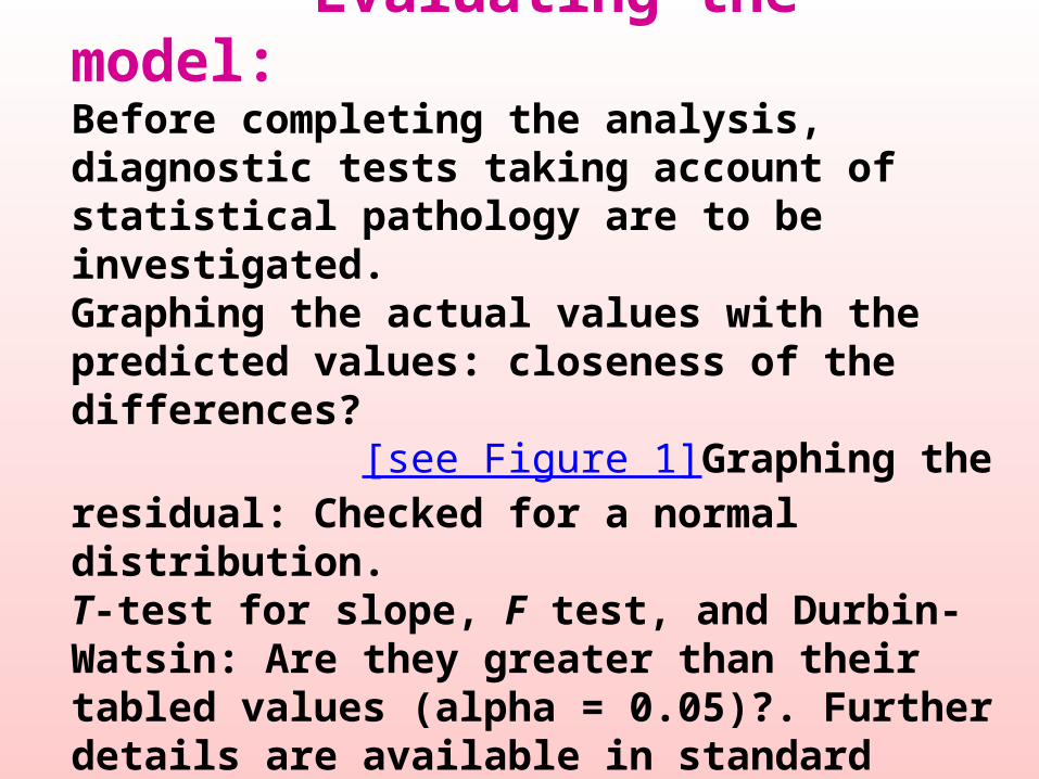
Evaluating the model:Before completing the analysis, diagnostic tests taking account of statistical pathology are to be investigated. Graphing the actual values with the predicted values: closeness of the differences? [see Figure 1]Graphing the residual: Checked for a normal distribution. T-test for slope, F test, and Durbin-Watsin: Are they greater than their tabled values (alpha = 0.05)?. Further details are available in standard texts (see references). An example, see Cho-Min-Naing et al (2000)

Discussion: 1.Epidemic of malaria: What? 1.1 Periodical rapid and great increase in malaria morbidity and perhaps mortality, reaching levels above local average endemicity.1.2 A rapid increase in malaria morbidity and mortality in a given population (independent of seasonal variations) which clearly surpasses.1.3 The usual levels, or the appearance of the infection in an area where it was not known before.A sharp increase of the incidence of malaria among a population in which disease was unknown.

Points to ponder:1. Among diverse factors, the selection of independent variables should be judiciously based on theoretical considerations. 2. It is worth emphasizing that the simple, two-variable regression model is limited in information. 3. The preferred approach is to perform regression model for more than one independent Variable. That is, multiple regression analysis: It allows the investigator to assess the separate effects of several unconfounded independent variables on a single dependent variable.

A cautionary note:For real progress, the

mathematical modeller as well as the epidemiologist must have

mud on his boots. [Bradley,1982].

References:

1. Armitage P, Berry G. Automatic selection procedures and colinearity. In:Statistical Methods in Medical Research. 3rd ed. Blackwell Scientific Publications, Oxford. 1994; 321-323.

2. Centred for Health Economics, Chulalongkorn University, Bangkok, Thailand. Lecture Notes on Econometrics. (1995/96) (unpublished) 3. Doti JL, Adibi E. Identifying and correcting econometric problems. In: Econometric Analysis: An Application Approach. Prentice-Hall, Inc, New Jersey. 1987; 203-265.

References (cont):4. Foster DP, Stine RA, Waterman RP. Summary regression case. In:Business Analysis Using Regression: A Case Book. Springer-Verlag New York, Inc. 1998; 227.

5. Gujarati DN. Test of specification errors. In: Basic Econometric. 3rd ed. Mcgraw-Hill, Inc. Singapore. 1995;461.

6. Kleinbaum DG, Kupper LL, Muller KE. Regression diagnostics. In: Applied Regression Analysis and Other Multivariable Methods. 2nd ed. PWS-KENT publishing Company. Boston. 1988: 181-225.

7. Roll Back Malaria. Malaria Early Warning Systems. WHO/CDS/RBM/2001.32. 2001