FLUID-STRUCTURE INTERACTION IN LIQUID- FILLED …atijssel/pdf_files/Lavooij-Tijsseling_1991.pdf ·...

Journal of Fluids and Structures (1991) 5, 573-595

FLUID-STRUCTURE INTERACTION IN LIQUID- FILLED PIPING SYSTEMS

C. S. W. LAVOOlJ AND A. S. TIJSSELING Delft Hydraulics, P.O. Box 177, 2600 MH Delft, The Netherlands and Delft University

of Technology, Department of Ovil Engineering, P.O. Box 5048, 2600 GA Delft, The Netherlands

(Received 9 November 1990 and in revised form 10 May 1991)

Fluid-structure interaction in liquid-filled piping systems is modelled by extended water hammer theory for the fluid, and beam theory for the pipes. All basic coupling mechanisms (Poisson, junction and friction coupling) are modelled. Two different solution procedures are presented. In the first procedure the governing set of equations is solved by the method of characteristics (MOC). In the second procedure the fluid equations are solved by the method of characteristics, while the pipe equations are solved by the finite element method in combination with a direct time integration scheme (MOC-FEM). The two procedures are compared with each other for a straight pipe problem. The MOC-FEM procedure is also verified against a solution procedure in which the pipe equations are solved by modal superposition.

The mathematical model is validated by simulation of two experiments known from literature: a straight pipe experiment and an experiment with one freely moving elbow. A provisional guideline is formulated which states when interaction is of importance.

1. I N T R O D U C T I O N INVESTIGATIONS OF RESEARCHERS IN THE PAST make clear that classical water hammer theory (Wylie & Streeter 1978) is sufficient and adequate to predict extreme loadings on a system, as long as it is rigidly anchored. However , when a piping system has certain degrees-of-freedom, severe deviations from classical theory may occur due to motion of the system. Pressure waves exert forces which cause a compliant system to move. The motion causes pressure waves in return. This phenomenon is called Fluid-Structure Interaction (FSI).

FSi is essentially a dynamic phenomenon. The interaction is always caused by dynamic forces which act simultaneously on fluid and pipe. It is convenient to classify the dynamic forces into two groups: distributed forces and local forces.

Distributed forces act along the pipe. The force caused by the fluid pressure is an example. Due to rapid pressure fluctuations a pipe expands or contracts, resulting in axial stress waves in the pipe wall. The stress waves in return generate pressure fluctuations in the enclosed fluid. This coupling is referred to as Poisson coupling. The generated pressure fluctuations are usually called precursor waves because they propagate faster than the 'classical' pressure waves. The forces caused by fluid friction are a second example of distributed forces. The mutual friction force is responsible for a coupling called friction coupling. In most practical systems this coupling is weak.

Local forces act at specific points of a system, such as elbows, tees or valves, and cause a structural motion that can be regarded as a pumping action. The motion generates pressure waves in the fluid. This kind of interaction is called junction coupling. In general it is dominant compared to Poisson and friction coupling.

The distinguished dynamic forces and their accompanying coupling mechanisms are diagrammed in Figure 1.

0889-9746/91/050573 + 23 $03.00 ~) 1991 Academic Press Limited

574 C. S. W. LAVOOIJ AND A. S. TIJSSELING

Interaction

1 Mutual dynamic forces

- -

I h Distributed forces Local forces

t l Friction coupling Junction coupling Poisson coupling

Figure 1. Diagram of forces causing fluid-structure interaction.

The research on FSI in fluid-filled pipes started many decades ago. A good survey of previous investigations is given by Wiggert (1986). A few important articles on which our work is based are still to be mentioned. Skalak (1956) and Lin & Morgan (1956) investigated the influence of FSI on pressure surges in straight pipes. Schwarz (1978) did an extensive numerical study on transients in straight pipes, including axial and radial inertia of the pipe wall. With respect to the research on FSI in complex piping systems, Wiggert & Hatfield (1983) formulated their Component Synthesis Method. This method couples the method of characteristics (MOC) for the fluid equations to a modal representation of the piping. Poisson coupling is not included in this method. We adopted Wiggert's idea of using a combination of the MOC and the finite element method (FEM) to solve the basic equations. However, we did not neglect the Poisson coupling.

The MOC is a powerful method to deal with wave phenomena. With respect to water hammer the method has many advantages: stability is firmly established, boundary conditions can be programmed easily, and complex systems can be handled. With respect to structural dynamics there is hardly any experience with the MOC. Wiggert et al. (1986) applied the MOC to Timoshenko beam theory and were partially successful. However, Vardy & Fan (1989) presented good results.

With respect to wave phenomena the FEM is less appropriate than the MOC. Due to partitioning of the pipe, only a limited number of fundamental frequencies can be described, so that steep wave fronts cannot be fully represented. On the other hand, as we shall see, only a limited number of frequencies is necessary to model the interaction. This is one of the reasons that the Component Synthesis Method is successful. To be able to deal with nonlinear systems in future, we integrate directly the transformed structural equations instead of using modal superposition.

Reviewing the various aspects of the MOC and the FEM we kept in mind the possibility of using existing software and knowledge as much as possible. Therefore, we decided to solve the fluid equations with the MOC and the structural equations with the FEM in combination with a direct integration scheme (Newmark fl = ¼). The Poisson coupling is included. Because of the fact that fluid and structural equations are coupled, an iteration over both solution methods is applied. In this paper we refer to this method as the MOC-FEM procedure.

To verify the MOC-FEM procedure, a straight pipe problem is solved by the MOC as well. The applied MOC procedure avoids the use of interpolations and is therefore described in detail.

FSI 1N LIQUID-FILLED PIPING SYSTEMS 575

2. BASIC E Q U A T I O N S

2.1. EXTENDED WATER HAMMER EQUATIONS

In water hammer theory the equations for momentum and continuity are applied to the mean flow. The flow is considered as one-dimensional and isothermal. The equations are

Momentum:

Continuity:

av f + g - Vr IVA, (1)

8t 8z 4R

8V g 8H 2VSOz -t - ( 2 )

8z c~ 8t E 8t '

in which c~ = Kf/pi(1 + 2RKJEe) -1. The other symbols are defined in the Nomen- clature (Appendix). By applying the stress-strain relations for a linearly elastic pipe, the continuity equation (2) can also be formulated in terms of fiz instead of Oz:

in which

8V g 8H 8fiz + - 2 v - - , (3)

8z c 2 8t 8z

__ 2RKr (1 - - c2= KY (1 + "V2)) 1.

To derive these equations (Schwarz 1978) it is assumed that:

• The one-dimensional description of the fluid flow is valid for pressure waves of low frequency. This assumption is known as the long wavelength approximation (Lin & Morgan 1956). As a result the radial inertia of the pipe wall can be neglected as well (Schwarz 1978).

• Convective terms can be neglected. Hence the fluid velocity is much smaller than the propagation speed of the pressure waves. This assumption is known as the acoustic approximation (Wylie & Streeter 1978).

• The friction can be modelled as if the flow were steady. With respect to FSI, the friction term in the momentum equation must be corrected for the axial motion, uz, of the pipe. For friction the relative fluid velocity Vr = V -- f~z is of importance.

• Cavitation does not occur. This means that the fluid pressure remains above vapour pressure.

• The pipe is linearly elastic and thin-walled.

In classical water hammer theory the terms on the right-hand side of the continuity equations (2) and (3) are neglected. This means that axial inertia of the pipe wall is neglected. Note that these terms are proportional to Poisson's ratio, v.

2.2. PIPE EQUATION FOR AXIAL MOTION

The governing equation for axial motion of the pipe reads

82Uz 28guz p fgSH+pfAy f v, lv, l + ( p i R + l ) g s i n y ' 8t 2 ct ~ Z 2 = •g p~e 8~ p,A--~ 4R pie

in which c~ = E / p ,

(4)


The continuity equations (2) or (3) and the axial pipe equation (4) are coupled via terms proportional to Poisson's ratio. These terms represent the Poisson coupling. The momentum equation (1) and the axial pipe equation (4) are coupled via terms proportional to the friction coefficient, f. These terms govern the friction coupling. Poisson coupling and friction coupling are modelled via the differential equations. Junction coupling is a result of local forces and therefore modelled via boundary conditions.

Equation (4) can be transformed to two first-order equations. Using tiz and o~ as variables the result is

3tiz 1 9Oz & A I f V~ IVrl + g sin y, (5)

8t Pt ~Z Pt A, 4R

~f~z 1 Oaz Rv 3H ~z ptc 2 0 ~ - & g e E 3t (6)

Note that equation (6) is a stress-strain relation differentiated with respect to time, with

3a~ R ~H 8t = p f g e ~7"

The derivation of equations (4), (5) and (6) can be found in Schwarz (1978).

2.3. BOUNDARY CONDITIONS

To obtain a solution for the set of equations formed by equations (1), (2) and (4) or the set formed by equations (1), (3), (5) and (6), boundary conditions are required. For the straight pipe problems to be discussed in Sections 4 and 5, the boundary conditions for a reservoir, a massless valve and axial impact are given.

2.3.1. Reservoir

The boundary conditions describing a constant head reservoir with a pipe rigidly connected to it, are

H = H .... (7a)

uz = 0, (7b)

where Hres is the pressure head at the reservoir.

2.3.2. Valve

The boundary conditions describing the instantaneous closure of a valve rigidly fixed to the ground are

V = 0, (8a)

Uz = 0. (8b)

The instantaneous closure of a valve which can move in the axial direction is modelled by

V = tiz, (9a)

Ataz = plgAf AH, (9b)

FSI IN LIQUID-FILLED PIPING SYSTEMS 577

in which AH is the pressure head difference over the valve. For a noninstantaneous valve closure, relations (8a) and (9a) are replaced by

V - tiz = 7:(t) A ~ , (10)

in which ~-(t) is a given function of time. For points of time greater than the closure time To, ~-(t) = 0.

2.3.3. Axial impact

When the closed end of a fluid-filled pipe is axially struck by a solid steel rod, as in the experiment described in Section 5, the boundary conditions during the period of contact are

V = ti z, ( l la)

Ataz = pigAiH + A r ~ r p r ( V - gor), ( l lb)

where V0r is the velocity of the rod just before impact. The subscript r denotes the properties of the rod.

3. NUMERICAL METHODS

The basic equations and boundary conditions given in the previous section are solved by two different solution procedures: the MOC -FE M procedure and the MOC procedure. Both procedures are discussed in detail.

3.1. THE MOC-FEM SOLUTION PROCEDURE

3. i. 1. Solution of the extended water hammer equations

If we consider H and V as the dependent variables, the basic equations (1) and (2) for the fluid form a set of hyperbolic partial differential equations. This hyperbolic set can be transformed to two sets of ordinary differential equations, which will be denoted as the C ÷ and C- equations

dI4 csdV fq 2,,c aOz ] - - + 0 , ( 1 2 a ) at g--d-f+4gR Vr[Vr[ gE at C+

dz = + cl; l (12b) dt

dH crdV fc I 2vc}Ooz 0 , ] (13a) dt g dt 4g---R Vr [Vrl gE at C -

dz d-~ = - c I. (13b)

Equations (12a) and (13a) are usually called the compatibility equations. Every solution of equations (12) and (13) is a solution of the original equations (1) and (2). No mathematical approximations have been made yet.

To derive finite difference equations, the pipe is divided into equal reaches of Az in length. The time step is chosen equal to At = Az/c r.

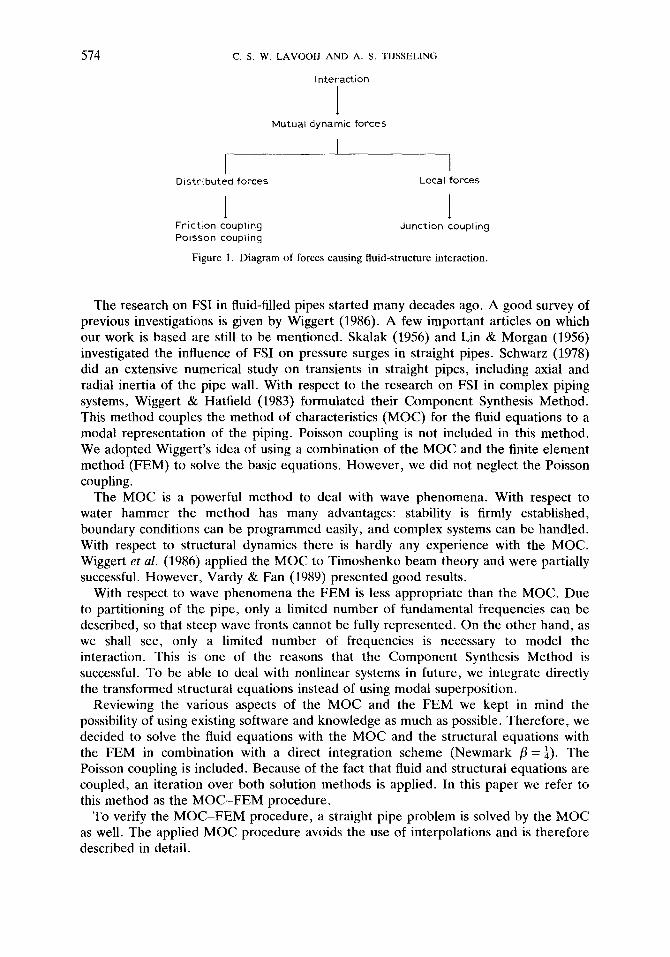
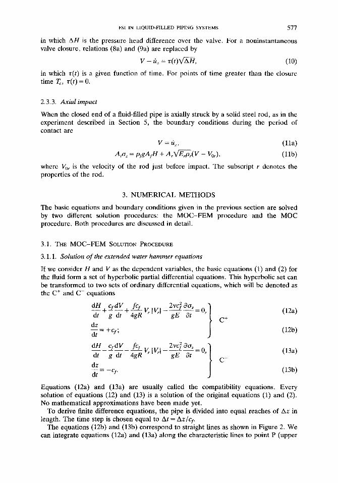
The equations (12b) and (13b) correspond to straight lines as shown in Figure 2. We can integrate equations (12a) and (13a) along the characteristic lines to point P (upper

57 8 C. S. W. LAVOOIJ AND A. S. TIJSSELING

n + l !

At ,n+112

,dz A E~ n ! I

i-1 i-112 i+112 +1

Figure 2. The (z, t)-plane with characteristic lines C + and C - .

index: time; lower index: place: o = oz):

C+: Hn+I-Hn_,+R*(VT+I-vn_I) TS*V~_ItV~ l [ - 2 T * ~ d t = O , (14)

f2 C-: H n+l Hi+ 1 R*(V~ +l VL1) S*V n 3or - " . . . . . , + , 1 v 7 . 1 1 - 2 r * ~ - d t = O, (15)

in which

R* = c_f, S* = fcf At T* = vc} g 4gR ' gE"

For the friction term, a first order approximation is likely to be satisfactory. The last terms in equations (14) and (15) can be estimated as follows:

fA P ~30"~ n+½ A t = O'n._+~ 1 3o /'/q- I

~ f dt = \ 3t/i-½ At ~ cri-½ At - cri%~' (16) Oin-~_

fP 30 / 3 0 \ n+½ n + l n O'i+½ -- O'i+½ n JB -~dt=~ At= A t = o;+? - oi+½. (17)

i+~ At

Hence the integrals are estimated by using the axial stresses at the mid-points of the elements. Equations (16) and (17) can be substituted in equations (14) and (15). Then H~ '+I (head in point P) and V n+l (velocity in point P) can be expressed in terms of all other variables.

If H and V are known at points A and B, the unknowns H and V in point P can be solved for in principle. However, Vr and cr z are not known a priori. The axial stresses Oz and velocities Vr are related to the pipe equations. Hence the solution of the pipe equations, by the FEM, must provide these variables.

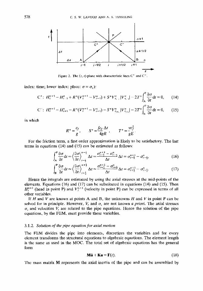
3.1.2. Solution of the pipe equation for axial motion

The FEM divides the pipe into elements, discretizes the variables and for every element transforms the structural equations to algebraic equations. The element length is the same as used in the MOC. The total set of algebraic equations has the general form

Mii + Ku = F(t). (18)

The mass matrix M represents the axial inertia of the pipe and can be assembled by


means of the so-called element mass matrices (Craig 1981). The same procedure can be followed for the axial stiffness matrix K and the load vector F.

To assemble M and K, standard subroutines from FEM libraries are used. For the time integration there was no software available for our purposes. To solve equation (18) we investigated two methods: the Newmark /3 method and the Wilson 0 method (Craig 1981). From the viewpoint of stability and accuracy, the Newmark fl = ~ method is a good choice. The method has no amplitude error (no numerical dissipation) and a small phase error. For multi-degree-of-freedom piping systems it is desirable to have some numerical dissipation to filter out disturbing higher modes. Particularly when the system is loaded by step loads (e.g. instantaneous valve closure), these higher modes produce an inaccurate response with numerically induced high frequency components. The Wilson method has numerical dissipation properties. Although the method is stable (depending on 0), it has the disadvantage of producing a larger phase error than the Newmark/3 = ¼ method.

When we tested both methods, we preferred the Newmark method because of its higher accuracy and because the method is unconditionally stable. To cope with high disturbing modes, a special form of Rayleigh damping was used. A damping matrix C was added to equation (18)

C = a0M + alK. (19)

The constants a0 and a 1 can be chosen to produce specific damping factors ~r for every mode r. It can be proved (Craig 1981) that the damping factors are a function of the eigenfrequencies ~or

X ( a° + al~o~ ). (20)

If we choose a0 = 0, the damping factors increase linearly with o9, In other words, the high frequencies are damped more than the low frequencies.

3.1.3. Solution algorithm

The steady-state solution of the basic equations will be the initial condition for the unsteady-state calculation. In a steady-state situation the basic equations are uncoupled. There are no dynamic forces involved. First, the fluid equations are solved for H and V. Second, the static load on the structure is determined and added to the structural equations. Finally the structural equations are solved for u.

After having solved the steady-state on t = 0, the dependent variables H, V and u on the next time step t = At are solved. To solve the fluid equations, the pipe variables must be known. However , the pipe variables depend on the fluid variables. Because we use two different numerical methods (MOC and FEM), an iteration over the solutions of the MOC (fluid) and the FEM (pipe) is necessary within each time step. The solution algorithm is as follows:

1. The axial stresses and axial pipe velocities are estimated by taking the values at the former time step.

2. The axial stresses and axial pipe velocities are transferred to the finite difference equations (14) and (15).

3. The finite difference equations (14) and (15) are solved for H and V. 4. H and V are transferred to the structural equation (18), the load vector F is built. 5. The structural equation (18) is solved for u by the Newmark/3 = ¼ method.

580 C.S.W. LAVOOIJ AND A. S. TIJSSELING

6. New axial stresses and axial pipe velocities are computed. 7. Return to step 2 if the solution of H, V and u has not attained the desired

accuracy. 8. Proceed to next time step (go to 1).

In this way the total set of equations is solved every time step. Using IHk+l - Hk[ < 0.001 m (k = iteration number) as a convergence criterion, solutions are attained within 10 to 15 iterations in case of instantaneous step loads.

3.2. THE MOC SOLUTION PROCEDURE

In this section, equations (1), (3), (5) and (6) are replaced by four equivalent equations which can be easily integrated. The integrations take place on a computational grid. The grid employed in this study substantially reduces the use of interpolations, which is of great advantage, as interpolations cause numerical damping. However, a slight adjustment of the wave speeds is necessary.

3.2.1. Compatibility equations

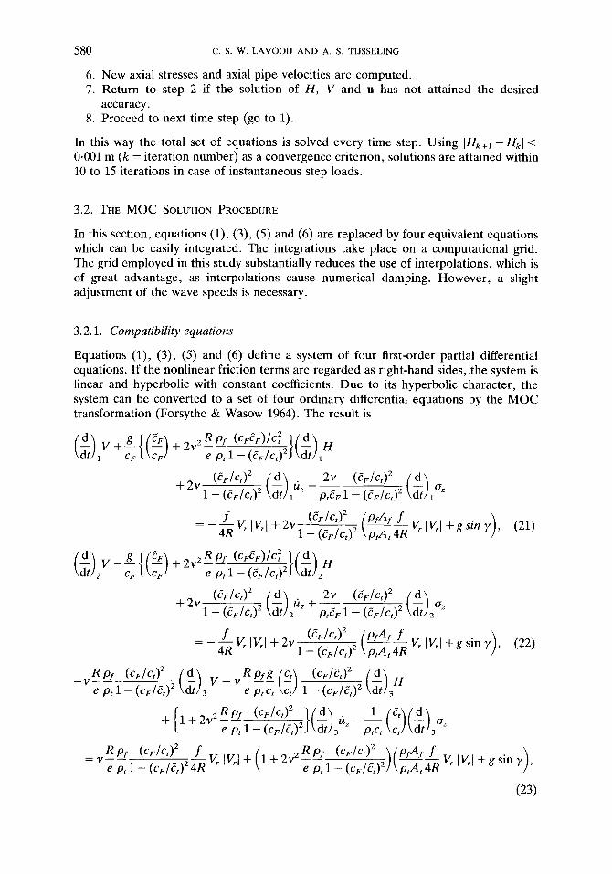
Equations (1), (3), (5) and (6) define a system of four first-order partial differential equations. If the nonlinear friction terms are regarded as right-hand sides, the system is linear and hyperbolic with constant coefficients. Due to its hyperbolic character, the system can be converted to a set of four ordinary differential equations by the MOC transformation (Forsythe & Wasow 1964). The result is

+ + " l-e (CF/Ct) 2 d 2v + 2V 1 _ ~ ) 2 ( ~ ) l f i z (CF/Ct ) 2 d

pt~F l -- (eF/c,)Z (-dt) l Oz

f Vr IVr[ +2~ (Cv/C')2 (pfAf f - 4R 1-__(~F]G)Z\ptAt~VrlVrl+gsiny], (21)

d v _ g eF & (c,X~)lc~ l i d \ (dt)2 CF{(CF )+ 2v2R e p , l = ~ 2 } ~ d t ) 2 H

(CF//C,) 2 d 2v (CFIICt) 2 d +2Vl:(~F/Ct)2(dt)ugtZ+pt~-Fl--(~F/Ct)2(dtt)20z

- f V~ IVr[ + 2v 1 (CF/C')2 (pfAf f y), (22) 4R - (~v/Ct) 2 \ P t A t - ~ Vr [Vrl + g sin

e p, l--(CF/G) 2 ~ V - v 3 eptct G l Z ~ ) 2 ~ 3

e p,I--(~F/G)EII~)3u~--p,c-~ ~ ~ 3 °z

R , f (CF/C,) 2 f { Rpy (CF/C,) 2 ~(piA, f = v - ~ E IEI + g s i n eptlT(~F/~t)2~-RVrlV~l+ 1 + 2 v 2 - - e p, 1 - (CF/G) 2 ] \ptA, -~ Y]'

(23)


--vRPYeptlZ(~F/Ct) 2(CF/ct)2 (d) V~ 4 -~- vRpfg(Ct)eDtct---- ~tt 1 Z ~ ) 2(cF/ct)2 (d) H~ 4

..[_ (1 _t_ 2V2 R pf (CF/Ct) 2 ~ ( d ~ l ~ 1 e t d e p t l - (Cv /~ t ) zJ ~dt]4 z-~ ptct (ctt)(d=t)40"z

R p f (CF/C,) 2 f ( ~ 2RP, (CF/C,) 2 \ ( p f A f f VriV, l + g s i n , ) = v VrlVrl+ 1 +

e p, 1 - (CF/6t)24R LV e ~ 1 -- (CF/6t)z)\p,At4R '

(24)

where (d/dr)l, (d/dt)z, (d/dt)3 and (d/dt)4 stand for the directional derivatives along the characteristic lines with slopes 1/gF, --1/gF, 1/~t and -116, respectively; in this context characteristic lines are lines in the (z, t)-plane along which disturbances propagate. The propagation speeds are

gF = [½{q2 _ (q4 _ 4C2FC~)½}]½ (25)

for the pressure waves in the fluid and

¢, = [½{q2 + (q4 _ 4c~c2)½}]½ (26)

for the axial stress waves in the pipe, with q2 = c 2 + (1 + 2vZpfR/El)cZF . Equations (21)-(24), called the compatibility equations, can easily be integrated.

The left-hand sides are integrated exactly, the nonlinear right-hand sides numerically. The ultimate result is that the vector of unknowns (V, H, tiz, az) at any point, P, in the interior (z, t)-plane is expressed in its values at four former points, A1, A2, A3, A4. The points At, Az, A3, A4 are situated on distinct characteristic lines. In Figure 3 they are taken one time step, At, earlier with respect to point P. It is concluded that the unknowns in any point, P, not on a boundary are fully determined, once initial and boundary values are given. For point P on a boundary, the boundary conditions have to be applied.

3.2.2. Computational grid

The computational grid generally used in classical water hammer theory (Wylie & Streeter 1978) is taken as a starting point (Figure 4). It is based on the characteristic lines along which the pressure waves propagate. The mesh spacings Az and At are constant. In this grid the points AI and A2 are grid points. The points A 3 and A4, however, generally fall between two grid points. Instead of estimating the values at A 3

A3 I

A I A2 A4

- - D , ~ E

Figure 3. Points P, A1, A2, A 3 and A 4 in the (z, t)-plane.

582 C. S. W. L A V O O I J A N D A . S. T I J S S E L I N G

AZ p I Jr

A 3 A1 A2 A4

Figure 4. Computational grid; (o, grid point).

i I I

l , i

P

i ii ilI :+ A 3 A 1 A 2 A4

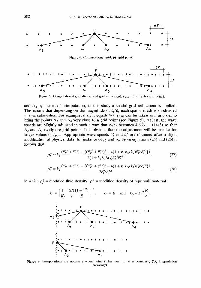
Figure 5. Computational grid after spatial grid refinement, iscR = 3; (I, extra grid point).

and m 4 by means of interpolation, in this study a spatial grid refinement is applied. This means that depending on the magnitude of 6t/6r each spatial mesh is subdivided in is~R submeshes. For example, if Ct/gF equals 4.7, isoR can be taken as 3 in order to bring the points m 3 and A 4 very close to a grid point (see Figure 5). At last, the wave speeds are slightly adjusted in such a way that 6t/er becomes 4 - 6 6 6 . . . (14/3) so that A3 and A+ really are grid points. It is obvious that the adjustment will be smaller for larger values of is~R. Appropriate wave speeds ~ and 5" are obtained after a slight modification of physical data, for instance of pf and p,. From equations (25) and (26) it follows that

(6~ 2 + 5 .2) + {(5~ 2 + 5*2) 2 - 4(1 + k,k3/k2)6~2~.*2}½ p• = kl 2(1 + klk3/k2)6~25 .2 , (27)

( 6 } 2 + g .2) - { ( 5 } 2 + 622) z - 4(1 + k,k3/k2)e~-25*2}½ o,* = k2 , ( 2 8 )

ZCF Ct

in which p~ = modified fluid density, p* = modified density of pipe wall material,

k l = { ~ f 4 2 R ( l ~ - v 2 ) } -1, k2=E and k3=21/2R e e

A 3

I • I I e l I + I +

~o I I 0" I I . I I ~ I I • ~ I I ®

/) A I A 2 A 4

• t I 0 T ; I I I • [ 1 Q I • r ®

A 2 A4

Figure 6. Interpolations are necessary when point P lies near or at a boundary; (O, interpolation necessary).


The time mesh is, except at boundaries, not divided into submeshes. A t and near boundaries interpolations are necessary for one of the four points A1, A2, A3, A4, as can be seen in Figure 6.

4. N U M E R I C A L V E R I F I C A T I O N ( S T R A I G H T PIPE)

To compare the solution procedures discussed in the previous section, both procedures are applied to the straight pipe system shown in Figure 7.

The fluid is flowing f rom reservoir to valve with a velocity of 1 m/s . The pressure behind the valve is 0 Pa. The pipe and the valve can freely move in the axial direction. To induce water ham m er the ball valve is closed instantaneously, that is to say within one time step, At = 0.5 ms. In Figure 8(a) the time function of the pressure head at the valve is shown. As can be seen in the legend, the densities of fluid and pipe material are slightly adjusted (compared to the original problem definition) in the M O C solution in order to avoid interpolations. In the M O C - F E M solution, 1% damping (based on o91) is used. The pressure heads according to both solution methods agree very well. The M O C - F E M solution shows overshoot and oscillations at times where the head changes sign. These phenomena are caused by the instantaneous valve closure, which is a discontinuity that cannot be handled proper ly by the FEM. Due to the partitioning of the pipe, only a limited number of modes can be described. To account for discontinuities, an infinite number of modes would be necessary.

Figure 8(b) shows the t ime functions of the pressure heads at the valve when the valve is closed in 30 ms. Now both solution methods give almost exactly the same result. Small differences can be observed due to the 1% damping used in the M O C - F E M calculation.

5. E X P E R I M E N T A L V A L I D A T I O N ( S T R A I G H T PIPE)

One of the best experiments with respect to FSI in a straight pipe is provided by Vardy & Fan (1989). The test rig consists of a 4.5 m long steel pipe suspended by wires. The pipe, which has an internal diameter of 52 m m and a wall thickness of 3-9 mm, is closed at both ends and filled with pressurized water. Stress waves in the pipe wall and pressure waves in the water are generated simultaneously by the axial impact of a solid steel rod at one of the pipe ends.

y Z

B Figure 7. Schematic of reservoir-pipe-valve system. Length = 20m, outer diameter= 813 ram, wall

thickness = 8 mm, Young's modulus = 21 x 10 l° N/m 2, density of pipe = 7900 kg/m 3, Poisson's ratio = 0.3, density of fluid= 1000kg/m, bulk modulus=21 × 10 N/m 2, friction coefficient=0.02, initial fluid

velocity = l m/s, pressure behind valve = 0 Pa.


200

150

100

50 " o

t -

O

b3 I l l

- 5 0 n

-100

- 1 5 0

Ca)

i

5

V - 2 0 0

o s'o 16o ~ o 200

Time (ms)

200

150

(b)

100

s o "0

¢-

0 L

m 113

P - 5 0 . iX.

- 1 0 0

-150

-2°°o ~6 16o 1~o 200 Time (ms)

Figure 8. Compar i son between M O C - F E M and M O C procedures for reservoir-pipe-valve system, Pressure head at valve for: (a) instantaneous valve closure; (b) valve closure within 30 ms. , M O C - F E M

(1% damping); - - - , M OC (isG R = 13, py* = 1000 kg /m 3, p* = 7898 kg/m3).


2.0 ¸

1.51 (a)

1.0

n 0-5

P 0

P [i.

-0,5

-1.O

-1-5

- 2 . 0 -,'- O 2 4 6 a io 12 14 16 18 2o 22

Time (ms)

I].. E

t, L 13.

2-0

1-5

1.0

0.5

0 - -

- O 5

-1 .0

-1.5

-2-0 0

t

J

(b)

I I

J I I

[ J / I I

i

;, ~, 6 ~, 1'o ;2 1:~ 1~ 1;3 2'0 22 Time (ms)

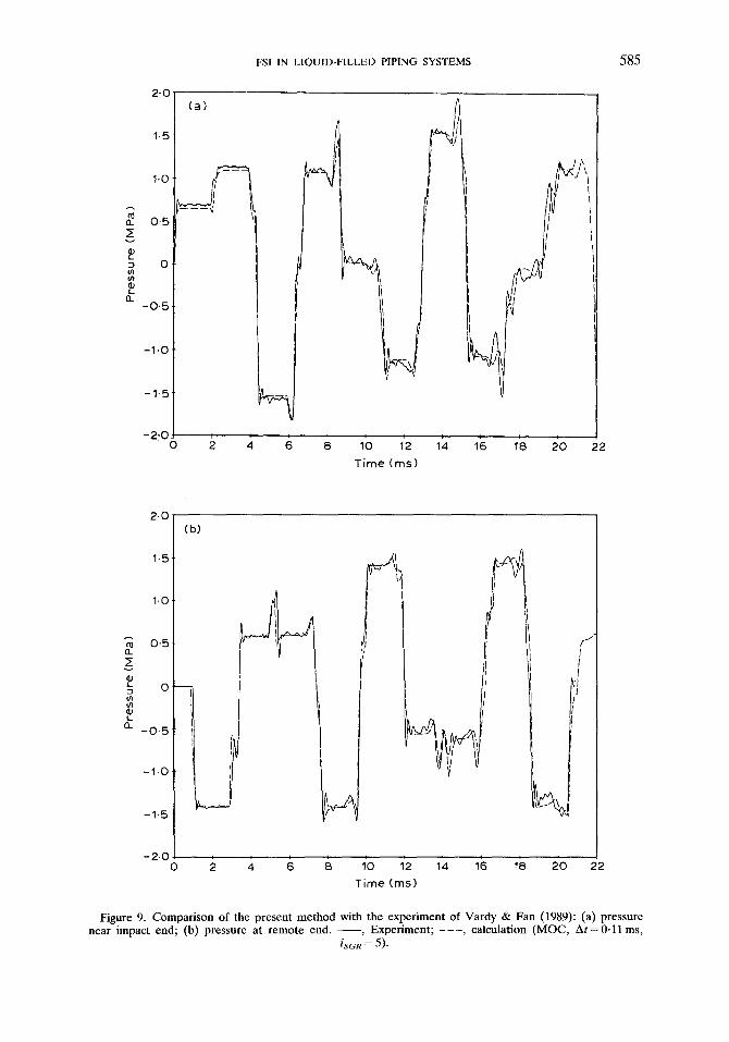
Figure 9. Comparison of the present method with the experiment of Vardy & Fan (1989): (a) pressure near impact end; (b) pressure at remote end. - - - , Experiment; - - - , calculation (MOC, At = 0.11 ms,

iSCR = 5).


Pressures, strains and pipe wall velocities were measured at various locations. The measured dynamic pressures at the pipe ends are shown in Figure 9, together with calculated results (MOC procedure with V0r = 0-739 m/s and isGn = 5). The agreement between measurement and calculation is excellent. The same degree of agreement was already found by Vardy & Fan (1989), who employed the MOC with time-line interpolations.

6. EXTENSION TO LATERAL AND TORSIONAL PIPE MOTION

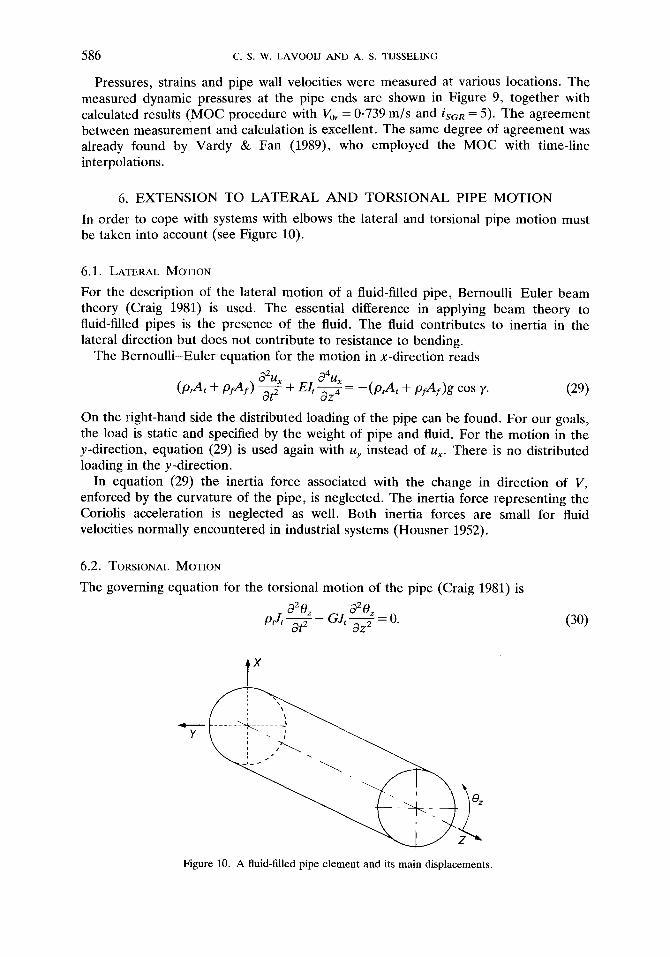
In order to cope with systems with elbows the lateral and torsional pipe motion must be taken into account (see Figure 10).

6.1. LATERAL MOTION

For the description of the lateral motion of a fluid-filled pipe, Bernoulli-Euler beam theory (Craig 1981) is used. The essential difference in applying beam theory to fluid-filled pipes is the presence of the fluid. The fluid contributes to inertia in the lateral direction but does not contribute to resistance to bending.

The Bernoulli-Euler equation for the motion in x-direction reads

02Ux 04Ux (ptAt 4- pfAf) ~ - 4- EI t Oz 4 = -(fltAt 4- pfAf)g cos ~/. (29)

On the right-hand side the distributed loading of the pipe can be found. For our goals, the load is static and specified by the weight of pipe and fluid. For the motion in the y-direction, equation (29) is used again with Uy instead of ux. There is no distributed loading in the y-direction.

In equation (29) the inertia force associated with the change in direction of V, enforced by the curvature of the pipe, is neglected. The inertia force representing the Coriolis acceleration is neglected as well. Both inertia forces are small for fluid velocities normally encountered in industrial systems (Housner 1952).

6.2. TORSIONAL MOTION

The governing equation for the torsional motion of the pipe (Craig 1981) is

O20z 320z P~l t - -~ - - GJ, ~zTz~ = O. (30)

T X

..-¢-

Figure 10. A fluid-filled pipe element and its main displacements.


The first term describes torsional inertia, the second torsional stiffness. There are no loads involved. The influence of fluid friction is neglected.

6.3. BOUNDARY CONDITION FOR AN ELBOW

A freely moving elbow will be considered as a boundary condition. Consider an elbow as shown in Figure 11. The elbow can be schematized as two pipe elements (1 and 2) connected in point P. If the mass balance is applied to the control volume the result is

(VAr)A - (tizZf)A = (VAy)B - (azAf)B. (31)

Because the elbow is considered as a point (control volume---> 0),

HA = HB. (32)

The above equations form an internal boundary condition for the fluid. Note that in equation (31) the structural variable, t~ z, occurs (junction coupling). Applying the momentum balance to the control volume, the forces on the adjacent pipes are

FA = p f g ( H A f )A, F B = p f g ( H A f ) B. (33a ,b )

The forces due to change in momentum (p iVZAf ) are neglected.

6.4. EXTENSION OF TIlE M O C - F E M SOLUTION PROCEDURE

The modelling of FSI for systems with one or more elbows is based on six differential equations: two equations for the fluid [equations (1) and (2)] and four equations for the pipe [equation (4), equation (29) for x- and y-direction and equation (30)].

The Bernoulli-Euler equations cannot be solved with the MOC solution procedure. To use the MOC procedure for lateral motion one has to apply Timoshenko beam theory. Application of the MOC solution procedure to Timoshenko beam theory has already been investigated by Leonard & Budiansky (1954), Chou & Mortimer (1967), Wiggert et al. (1987) and Vardy & Alsarraj (1989). The authors are still investigating this subject.

P

VA Im //z I /

• ~VE,

2 I

Figure 11. Schematic of an elbow.

Control volume


A ~ZO,y ~ C

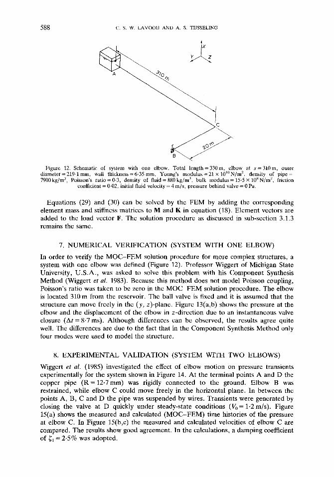
Figure 12. Schematic of system with one elbow. Total length = 330m, elbow at s = 310m, outer diameter = 219.1 mm, wall thickness = 6-35 mm, Young's modulus = 2l × 101° N / m 2, density of pipe = 7900 kg/m 3, Poisson's ratio = 0.3, density of fluid = 880 kg]m 3, bulk modulus = 15-5 × 108 N/m 2, friction

coefficient = 0-02, initial fluid velocity = 4 m/s , pressure behind valve = 0 Pa.

Equations (29) and (30) can be solved by the FEM by adding the corresponding element mass and stiffness matrices to M and K in equation (18). Element vectors are added to the load vector F. The solution procedure as discussed in sub-section 3.1.3 remains the same.

7. NUMERICAL VERIFICATION (SYSTEM WITH ONE ELBOW)

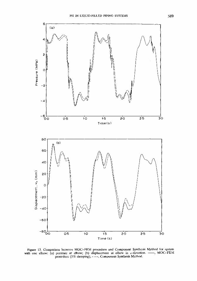
In order to verify the MOC-FEM solution procedure for more complex structures, a system with one elbow was defined (Figure 12). Professor Wiggert of Michigan State University, U.S.A., was asked to solve this problem with his Component Synthesis Method (Wiggert et al. 1983). Because this method does not model Poisson coupling, Poisson's ratio was taken to be zero in the MOC-FEM solution procedure. The elbow is located 310 m from the reservoir. The ball valve is fixed and it is assumed that the structure can move freely in the (y, z)-plane. Figure 13(a,b) shows the pressure at the elbow and the displacement of the elbow in z-direction due to an instantaneous valve closure (At = 8.7 ms). Although differences can be observed, the results agree quite well. The differences are due to the fact that in the Component Synthesis Method only four modes were used to model the structure.

8. EXPERIMENTAL VALIDATION (SYSTEM WITH TWO ELBOWS)

Wiggert et al. (1985) investigated the effect of elbow motion on pressure transients experimentally for the system shown in Figure 14. At the terminal points A and D the copper pipe ( R = 12-7mm) was rigidly connected to the ground. Elbow B was restrained, while elbow C could move freely in the horizontal plane. In between the points A, B, C and D the pipe was suspended by wires. Transients were generated by closing the valve at D quickly under steady-state conditions (V0 = 1-2 m/s). Figure 15(a) shows the measured and calculated (MOC-FEM) time histories of the pressure at elbow C. In Figure 15(b,c) the measured and calculated velocities of elbow C are compared. The results show good agreement. In the calculations, a damping coefficient of ~1 = 2-5% was adopted.


°l (a)

E

u~

n

4 ¸

2 ¸

0

- 2

t

i r \ '

- 6 1 0.0 0'.5 1'. 115 210 2'.5 3 . T i m e ( s )

8 0 (b)

, o

40 !

"E 20 E

0

E o - 2 0 f~

5_ v1

c~ - 4 0

- 6 0

-8O5o 015 ~.'0 ~5 210 2'.5 310 T i m e (s)

Figure 13. Comparison between MOC-FEM procedure and Component Synthesis Method for system with one elbow: (a) pressure at elbow; (b) displacement at elbow in z-direction. - - , MOC-FEM

procedure (5% damping); - - - , Component Synthesis Method.

590 c. S. W. LAVOOIJ AND A. S. TIJSSELING

----- t B~ 2 8 - 0 2 m - - } = ~ _ _ _

A vo= l 2 m / s

oA 12,27 m C

Figure 14. Schematic of the test circuit used by Wiggert e t al. (1985).

7-65 rn

~z l

Uz2

9. WHEN IS FLUID-STRUCTURE INTERACTION IMPORTANT?

A most relevant question with respect to practice is: when is FSI important? We will try to answer this question by formulating a provisional guideline. Another

question which arises is whether Poisson coupling is important or not. This question has never been paid much attention to in the literature. Reviewing the three coupling mechanisms, one can imagine that friction coupling is the least important. We will concentrate here on junction and Poisson coupling.

In order to investigate the influence of interaction, the system with one elbow (Figure 12) was solved in three different ways: (a) Uncoupled

All three types of coupling are neglected. There is no feed-back from the structural motion to the fluid. Poisson's ratio is set to zero.

(b) With junction coupling Only Poisson coupling is neglected (v = 0).

(c) With junction and Poisson coupling All types of coupling are taken into account.

Here we will discuss results with valve closure times, Tc = 0.5 s and Tc = 1.5 s.

9.1. Tc = 0.5s

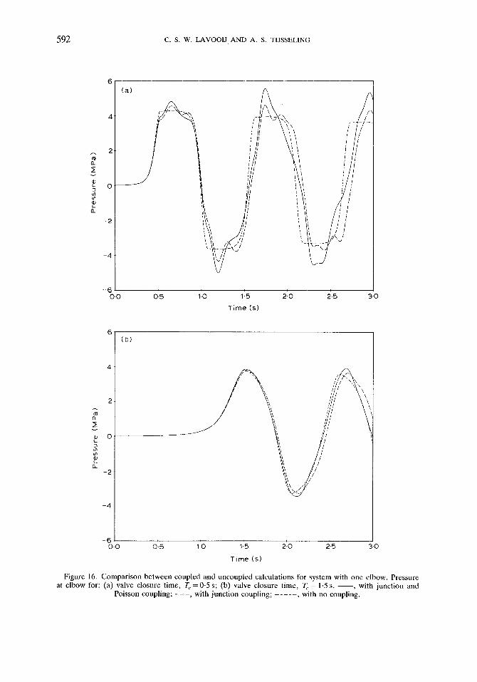
For the coupled calculations the pressure at the elbow [Figure 16(a)] clearly shows the influence of structural frequencies. The axial natural frequency of the long leg is about 4 Hz. Due to junction coupling this frequency can be recognized in the pressures as well.

It is of interest to investigate some time scales of this problem. The main time scale of the water hammer waves, Tw = 4L/c I = 1.1 s. The effective closure time, T, el, of the valve is about 30% of the total closure time, thus Tcef = 0"15 S. Because T, ei< Tw, water hammer is of importance in this problem. To judge whether interaction is important, the eigenperiods, Ts, of the structure should be compared with Tcel and Tw. In this case the dominant Ts = 0-25 s, and thus

Teef < T~. < Tw. (34)

We believe that if the time scales satisfy this condition, FSI is important. Therefore equation (34) is adopted as a provisional guideline.

The natural mode of the system (fs = 4 Hz) is clearly dominated by the axial motion of the long leg. It seems logical to conclude that this is the reason why Poisson coupling is important in this problem as can be seen in Figure 16(a).

Hence we state that Poisson coupling is important if the modes which satisfy equation (34) are dominated by axial stiffness.


2 0 0 0

1 5 0 0

1 0 0 0

500

0 ¸

- 5 0 0 0

I \ '~ /\

~V, " " W

t

20 40 60

T i m e (ms)

8 0

E

-:3

0 - 5 0

0 .25

- 0 . 2 5

-0.50 0

(b)

- I V' y,,

20 40 60

Time (ms )

80

E v

' : 3

0 . 5 0 I

0-25 1

(c)

- 0 . 2 5

- 0 -50 0 20 40 60 80

T ime (ms)

Figure 15. Comparison of present method with experiment of Wiggert et al. (1985): (a) pressurc at valve; (b) pipe velocity at elbow in zl-direction; (c) pipe velocity at elbow in zz-direction. - - . , Experiment; . . . . ,

Calculation (MOC-FEM).

592 C. S. w . LAVOOIJ AND A. S. TIJSSELING

6 ] (a )

n

E

- 2

- 4

\ / / /

' I ~ ; i !

I~ ]/ I \ 71 I i

I I ~ /

- 6 1 q I o.o o'.s 1-o 1.s 2:0 2'-s 3.0

T i m e (s)

n

E

n

- 2

- 4

( b )

,<,' \ ' , / /// \ 1 //i

/ J

- 6 0.0 015 i.'0 11m 210 2.~ 3-0

T i m e (s )

Figure 16. Compar i son be tween coupled and uncoupled calculations for system with one elbow. Pressure at e lbow for: (a) valve closure t ime, T c = 0-5 s; (b) valve c losure t ime, T c = 1-5 s. - - , with junct ion and

Poisson coupling; - - - , with junct ion coupling; . . . . . , with no coupling.


9.2. T~ = 1-5 s

To perform a first check on the guideline, the valve is closed in 1.5 s instead of 0.5 s. Hence Tcei = 0.5 s (30% of 1.5 s). If we apply the guideline to this case it follows that: Te~1> T~ and hence the time scales do not satisfy condition (34). The guideline states that interaction is not important. This statement is confirmed by Figure 16(b) which shows the calculated pressures at the elbow.

10. REVIEW AND CONCLUSIONS

To model fluid-structure interaction (FSI) in liquid-filled piping systems the extended water hammer equations are used to model the fluid, and beam theory is used to model the structure. All basic types of coupling are modelled. The most significant coupling mechanisms are Poisson coupling and junction coupling.

In order to solve the basic set of equations the MOC -FE M solution procedures is formulated. The fluid equations are solved by the MOC (method of characteristics) and the structural equations are solved by the FEM (finite element method). The structural equations are integrated directly with the Newmark /3 =-14 method. To filter out disturbing high modes, a special form of Rayleigh damping is used.

For straight pipe problems the MOC-FEM solution procedure is compared with an MOC solution procedure. These tests show that, for pressure gradients of order time step At, the MOC procedure is more accurate. The MOC -FE M procedure remains stable. If the pressure gradient is built up over several time steps, the MOC-FEM procedure yields almost exactly the same results as the MOC procedure.

For m o r e complex piping systems the MOC-FEM procedure is compared with Wiggert's Component Synthesis Method. The results agree very well. Only junction coupling could be tested this way, because the Component Synthesis Method does not contain the Poisson coupling. However, in the Component Synthesis Method the Poisson coupling could be modelled in the same way as described in this paper.

To validate the mathematical FSI model two experiments were simulated: one concerning a straight pipe (Vardy & Fan 1989), and one concerning a system with two elbows (Wiggert et al. 1985). The agreement obtained between experiment and simulation is very good. It must be remarked that the experiments did not include torsional motion.

On the basis of our simulations we formulated a simple guideline which states when interaction is important. The guideline is formulated in terms of three time scales: the effective closure time of the valve, the eigenperiods of the structure and the time scale of the water hammer waves.

More simulations and experiments are necessary to test whether this provisional guideline is adequate. However, the guideline explains why in the Component Synthesis Method only a few modes are sufficient to model FSI quite accurately, namely: those modes which satisfy the guideline.

Poisson coupling is important for the fluid when significant modes for interaction are dominated by axial stiffness.

11. ACKNOWLEDGEMENTS

This work has been part of the FLUSTRIN project, initiated by Delft Hydraulics, The Netherlands.

The FLUSTRIN project is financially supported and guided by: (The Netherlands) Shell Internationale Petroleum Maatschappij B.V.; DSM Research; Ministry of Social


Affairs and Employment , Nuclear Department and Pressure Vessel Division; National Foundation for the Coordination of Maritime Research; Witteveen & Bos, Consulting Engineers; Public Works of Rotterdam; Mokveld Valves B.V.; Publiek Ontwerp; (Germany) Rheinisch-Westffilischer TUV; (UK) Powergen; ICI; Nuclear Electric; (France) Bergeron Rateau; Elf Aquitaine.

REFERENCES

CHou, P. C. & MORTIMER, R. W. 1967 Solution of one-dimensional elastic wave problems by the method of characteristics. Journal of Applied Mechanics 34, 445-450.

CRAIG, R. R., JR 1981 Structural Dynamics. New York: John Wiley & Sons. FORSWrHE, G. E. & WASOW, W. R. 1964 Finite-Difference Methods for Partial Differential

Equations. New York: John Wiley & Sons. HOUSNER, G. W. 1952 Bending vibrations of a pipe line containing flowing fluid. Journal of

Applied Mechanics 19, 205-208. LEONARD, R. W. & BUDIANSKY, B. 1954 On traveling waves in beams. National Advisory

Committee for Aeronautics, NACA Report 1173. LIN, T. C. t~ MORGAN, G. W. 1956 Wave propagation through fluid contained in a cylindrical,

elastic shell. Journal of the Acoustical Society of America 28, 1165-1176. SCHWARZ, W. 1978 Druckstossberechnung unter Beriicksichtigung der Radial- und

L~ingsverschiebungen der Rohrwandung. Universit/it Stuttgart, Institut flit Wasserbau, Mitteilnngsheft 43 (in German).

SKALAK, R. 1956 An extension of the theory of waterhammer. Transactions of ASME 78, 105-116.

VARDY, A. E. • ALSARRAJ, A. T. 1989 Method of characteristics analysis of one-dimensional members. Journal of Sound and Vibration 129, 477-487.

VARDY, A. E. & FAN, D. 1989 Flexural waves in a closed tube. In Proceedings of the 6th International Conference on Pressure Surges, pp. 43-57. Cambridge, U.K., BHRA.

WIGGERT, O. C. t~ HATFIELD, F. J. 1983 Time domain analysis of fluid-structure interaction in multi-degree-of-freedom piping systems. In Proceedings of the 4th International Conference on Pressure Surges, pp. 175-188. Bath, U.K., BHRA.

WIGGERT, D. C., OTVCELL, R. S. & HATFIELD, F. J. 1985 The effect of elbow restraint on pressure transients. ASME Journal of Fluids Engineering 107, 402-406.

WIOOERT, D. C. 1986 Coupled transient flow and structural motion in liquid-filled piping systems: a survey. In Proceedings International Conference on Computers in Engineering. New York: ASME, Division of Pressure Vessels and Piping.

WIGGERT, D. C., HATFIELD, F. J. t~z LESMEZ, M. W. 1986 Coupled transient flow and structural motion in liquid-filled piping systems. In Proceedings of the 5th International Conference on Pressure Surges, pp. 1-9. Hanover, Germany, BHRA.

WIGGERT, D. C., HATFIELD, F. J. t~L STUCKENBRUCK, S. 1987 Analysis of liquid and structural transients by the method of characteristics. ASME Journal of Fluids Engineering 109, 161-165.

WYLIE, E. B. t~L STREETER, V. L. 1978 Fluid Transients. New York: McGraw-Hill.

a~ Ar At ao, al C CF, Cf ~E ~7 Ct

eF E

A P P E N D I X : N O M E N C L A T U R E

cross-sectional discharge area cross-sectional rod area cross-sectional pipe wall area Rayleigh damping constants damping matrix pressure wave speeds (classical) pressure wave speed adjusted pressure wave speed axial stress wave speed (classical) axial stress wave speed adjusted axial stress wave speed Yonng's modulus for pipe wall material

FSI IN LIQUID-FILLED PIPING SYSTEMS

Er Young's modulus for rod material e pipe wall thickness F force vector F magnitude of force f Darcy-Weisbach friction coefficient f~ structural frequency G shear modulus for pipe wall material g gravitational acceleration H fluid pressure head Hr.s pressure head at reservoir I second moment of cross-sectional area iSGR spatial grid refinement factor J polar moment of inertia K stiffness matrix Ky fluid bulk modulus L pipe length M mass matrix P fluid pressure R internal radius of pipe s distance along the pipe Tc closure time of valve Tcer effective closure time of valve T~ eigenperiod of structure Tw water hammer time scale t time u displacement of pipe t~ velocity of pipe // acceleration of pipe V velocity of fluid Vr relative velocity of fluid Vo initial velocity of fluid Vo, initial velocity of rod x, y lateral coordinates z axial coordinate ), elevation angle of pipe AH pressure head difference over valve At numerical time step, mesh spacing Az element length, mesh spacing ~r damping coefficient 0z angular displacement v Poisson's ratio Pr fluid density Pr* modified fluid density Pr density of rod material Pt density of pipe wall material p* modified density of pipe wall material

given function of time az axial pipe stress a~ hoop stress tot eigenfrequency

595

FLUID-STRUCTURE INTERACTION IN LIQUID- FILLED …atijssel/pdf_files/Lavooij-Tijsseling_1991.pdf ·...

Documents

Transcript of FLUID-STRUCTURE INTERACTION IN LIQUID- FILLED …atijssel/pdf_files/Lavooij-Tijsseling_1991.pdf ·...