A Fluid-Structure Interaction Model for the Study ofEarthquake Response in a Dam-Water System

Ricardo Manuel Melo FariaDecember, 2014

Abstract − How a structure behaves in response to anearthquake is a decisive question when such an incidenthappens, in particular in heavy seismic hazardous regionsor for structures that require constant monitoring. This prob-lem has been typically addressed from a Solid Mechanicsperspective. Since a dam-water system consists in fact ina fluid-structure interaction problem, the usual EarthquakeEngineering approaches focused mostly on the analysis ofthe structure may not be the most adequate. Fluid Mechanicsplays an essential role here in order to have a robust andrealistic mathematical modelling of the problem and obtainsolid numerical simulations, the two main focus of this article.

1 Introduction

Throughout History, several records show that earth-quakes have always played a significant impact in societieswhen they occurred. The Great Lisbon Earthquake (1st ofNovember 1755), which left great part of Downtown Lisbondestroyed, is an absolute example of such impact in a timewhere no means to effectively face such a tragedy and littleknowledge about this phenomenon existed. From here camethe first efforts to understand and respond to earthquakephenomena in a large area: modern Seismology was born.

Along with the study of earthquake phenomena comesthe need to study how structures respond to it individually,in particular in heavy seismic hazardous regions and alsofor structures that require constant monitoring, which derivesfrom practical motivations like improving infrastructure design,construction and control. Such problem has been typicallyaddressed from a Solid Mechanics perspective, since themost common situation is to have a single solid structure.

The problem that is the subject of study in this work con-sists of a dam-water system. A dam is a barrier that im-pounds water or underground streams and often work asa hydropower system to generate electricity. For instance,such big and important engineering structures require con-stant monitoring, in particular checking if there exist cracksforming in the concrete and measuring water pressure along-side the dam-water wall. Since this problem is in fact afluid-structure interaction problem, the usual techniques fromSolid Mechanics and Earthquake Engineering alone are notthe most adequate, which is the main motivation for the workof this dissertation.

In this sense, Fluid Mechanics plays an essential rolehere, since appropriate equations that model fluid behaviourmust be taken into account in a more realistic mathematicalmodelling of the problem. A pressure-displacement formu-lation is suggested in [1], wherefrom we start by simplifying

the equations for the fluid. This is done by considering someproposed approximations for the pressure [1, 13]. From thisformulation we obtain a coupled system of equations thatallows us to consider usually overlooked physical phenom-ena, such as a wavelike motion on the water surface and theconsideration of interface conditions on the dam-water inter-face wall. These latter conditions are of special relevance,since they allow the coupling of equations (because of themathematical interdependence of variables).

We proceed with the derivation of the variational formula-tion of the problem following [2, 5] which allows us to brieflystudy properties for the solutions of the equations by a changeof variables for the pressure function. In addition, we considerthe associated stationary problem and prove existence anduniqueness of solution in this case. Afterwards we pass tothe numerical resolution of the problem. First we discretizethe equations in space and finish using a state space rep-resentation of the problem [10] followed by integration overtime through the integral form of the solution equation.

Next we regard the simulations and discussion of resultshaving used as input data the accelerogram of the 921 Earth-quake, also known as Chichi Earthquake. The computationalmethods used for purposes of this paper were entirely writtenand implemented from scratch in Matlab based on a scriptfor a structure-structure model following [11].

One of the positive aspects of this formulation is the lessdense dimension of the final system of equations. Introduc-tion of the pressure variable instead of displacements in partof the domain reduces the problem’s dimension considerably,and therefore also the number of necessary computations.This is indeed important for it is known that in very refined(dense) 3-D meshes, models formulated in displacementsstart to tackle some computational issues.

Main Results

The most important contributions of this paper are:

• the introduction of a pressure-displacement formulationalong a detailed mathematical modelling of the equa-tions governing the behaviour and earthquake responseof a dam-water system;

• the derived the energy estimates for the solutions of theweak equations;

• the computational implementation of the Finite ElementMethod from scratch in Matlab;

• the numerical simulations that have proven to have abetter execution runtime and demonstrate the possibil-ities in considering such a model in further research,namely for 3-D geometries;

1

Outline of this Paper

This paper is organized in 5 sections. Section 1, whichcorresponds to this Introduction, outlines the motivations andwhat is accomplished in this work. Section 2, first describesthe problem’s geometry, and from there it comprehends all themathematical modelling on physical phenomena for obtainingthe equations for the problem. In Section 3,, we start withsome Functional Analysis results and then focus on the varia-tional analysis of the problem and study of energy estimates.Description of the discretization of the problem, transitioningfrom an analytical continuous problem to a numerical anddiscrete one happens in Section 4. Finally, in Section 5 weshow performed simulations and actively discuss the resultswith insight for future work.

2 Mathematical Modelling of the Problem

We begin by considering a space domain D that com-prises a generic dam-water system for the derivation of theequations. We will refer to the dam as the structure and to thewater as the fluid. For obvious reasons, D ⊂ R3, although it ispossible to study a 2-dimensional model too, i.e., to considerD ⊂ R2. Our approach here consists of taking a profile of adam-water system on the xOz plane that we call Ω, such thatΩ ⊂ R2 and presenting the following sketch:

Figure 1: Sketch of the problem’s domain Ω along with itsgeometry.

Clearly there are two distinct regions in Ω, one the struc-ture itself Ωs, the other occupied by the fluid Ωf . As for theboundaries of these subdomains we have: Γ1 is the interfaceboundary between both Ωs and Ωf ; Γ2 is simply the groundor rock mass under the fluid; Γ3 is the fluid surface or theair-fluid interface; Γ4 is an artificial ’wall’ or delimitation ofthe fluid domain’s extension; Γ5 is the rock mass under thestructure; and finally Γ6 is constituted by the structure wallswith no contact with the fluid.

In addition, as we will be dealing with a dynamic problem,we must also consider a time interval domain [0, T ], whereT is a real positive, during which the dynamic fluid-structureinteraction occurs.

2.1 Coupled System of Equations

Assuming viscous effects by which deviatoric stresses areinduced can be neglected [1] in the Navier-Stokes equations,the motion of the fluid (in this case water) under the actionof gravity and seismic activity can be described by the Eulerequations. By also assuming that [1]

• the fluid mass density varies very little, so it may beconsidered constant %f ;

• velocities are small enough for convective effects tobe neglected;

we are able to linearize the system about the state of hydro-static equilibrium obtaining a single equation for the fluid inΩf only depending on its pressure. Although we considerthe fluid mass density as constant %f , we do not take its timederivative simply as null in Ωf×]0, T ]. The advantage in doingso is ending up with a flexible structure-compressible fluidmodel, as it will be obvious later [7].

Then, from the Navier equation for the structure under theaction of gravity and seismic activity we obtain an equationmodelling the motion of the structure in Ωs×]0, T ].

Putting everything together and deriving appropriate con-ditions for the fluid and the structure domain boundaries∂Ωf = Γ1 ∪Γ2 ∪Γ3 ∪Γ4 and ∂Ωs = Γ1 ∪Γ5 ∪Γ6, respectively,(so the behaviour of the fluid and structure falls under coher-ent descriptions of fluid and structure motion phenomena)we obtain the coupled system of equations that models thefluid-structure interaction in response to earthquake waveswritten as:

find ~u and p such that

∂2p

∂t2= c2∆p in Ωf×]0, T ]

%s∂2~u

∂t2= ∇ · (σ (~u))− ca

∂~u

∂t+ %s (~g + ~as) in Ωs×]0, T ]

∂p

∂nf= −%f

∂2~u

∂t2· ~ns on Γ1×]0, T ]

σ (~u)~ns = p~ns on Γ1×]0, T ]

∂p

∂nf= 0 on Γ2×]0, T ]

∂2p

∂t2= −g ∂p

∂nfon Γ3×]0, T ]

∂p

∂t= −c ∂p

∂nfon Γ4×]0, T ]

~u = 0 on Γ5×]0, T ]

σ (~u)~ns = 0 on Γ6×]0, T ]

(2.1)

p∣∣t=0= p0 in Ωf × 0

~u∣∣t=0= u0 in Ωs × 0

∂p

∂t∣∣∣t=0

= q0 in Ωf × 0

∂~u

∂t∣∣∣t=0

= v0 in Ωs × 0,

2

where p = p(x; t) is the (unknown) fluid pressure, ~u = ~u(x, t)

is the (unknown) structure displacement vector, σ = σ(~u) isthe structure Cauchy stress tensor, %f and %s are respectivelythe fluid and structure mass densities, c is the speed of soundin the fluid, ca is a positive constant representing the dampingeffect, g is the gravitational acceleration and ~as = ~as(t) is theacceleration of the ground due to earthquake waves.

The initial conditions ~u0, ~v0, p0 and q0 are assumed tobe sufficiently regular. Regularity conditions and adequatefunctional spaces for ~u and p will be discussed later.

We highlight now the conditions taken on Γ1, the interfaceboundary between the fluid and structure domains Ωf andΩs, respectively. Indeed, any displacement of the structureover time implies it acquires a certain velocity (thus motion)and acceleration, which is transferred to the fluid across Γ1

and vice-versa. Both these conditions, presented in System(2.1), come from imposing

~vf · ~nf = ~vs · ~ns on Γ1×]0, T ],

σf · ~nf = σs · ~ns on Γ1×]0, T ],(2.2)

where ~vf (resp. ~vs) is the velocity of the fluid (resp. structure),σf (resp. σs) is the fluid (resp. structure) Cauchy stress tensorand ~nf (resp. ~ns) is the outward unit normal vector to Ωf

(resp. Ωs). The first condition means that the fluid and thestructure must have the same velocity in the normal directionon Γ1, so the motion of both bodies couples successfully. Thesecond just implies that the stress tensors of the fluid and thestructure must be equal on Γ1 as well.

3 Functional Framework for the Problem.Variational Formulation. Weak Solutions

Let us clarify some notations used hereafter [2, 4, 5].We write ‖f‖p,Ω to refer to the usual Lebesgue norm for

f ∈ Lp(Ω). With the same reasoning , ‖u‖m,p,Ω is the usualnorm in the Sobolev space Wm,p(Ω). It is well known that,in particular, for p = 2 and m ≥ 0 we have that the spaceHm(Ω) := Wm,2(Ω) is a Hilbert space. We remark the spe-cial case H1

Γ(Ω), the space of functions in u ∈ H1(Ω) thatare null on a boundary portion Γ ⊂ ∂Ω, in which ‖∇u‖2,Ωalso constitutes a norm by applying Poincaré’s Inequality [4].Finally, if X is a Banach space, ‖u‖Lp(a,b;X) is the usual normtaken in the Bochner space Lp(a, b;X) and D′(a, b;X) is thespace of distributions defined in [a, b] with values in X.

3.1 Function Spaces for Solutions

In order to derive the variational formulation of Problem(2.1), next we choose test functions ~ϕ = ~ϕ(x) ∈ Vs (withrespect to ~u) and ψ = ψ(x) ∈ Vf (with respect to p). Nowwe must define precisely what are the test-function spacesVf and Vs, so we know exactly where we will be lookingfor solutions in what concerns the spacial variable. We setd := dim(Ω), which in our case takes the value d = 2.

In the fluid equation, since there are only Neumann bound-ary conditions on ∂Ωf , it suffices to define

Vf = H1(Ωf ) := ψ ∈ L2(Ωf ) : ∇ψ ∈ L2(Ωf )d, (3.1)

for it is natural that Neumann boundary conditions appear inthe weak form equations themselves.

For the structure equation, we have a Dirichlet boundarycondition on Γ5 ⊆ ∂Ωs, so we must impose

Vs = ~ϕ ∈ L2(Ωf )d : ∇~ϕ ∈ L2(Ωf )d×d

∧ ~ϕ = 0 on Γ5. (3.2)

It is acknowledged that (homogeneous) Dirichlet boundaryconditions must always be imposed in the test functionsspaces, since they do not appear in the weak formulationany other way.

3.2 Variational Formulation of the Problem

Deriving now the the variational formulation for Problem(2.1), we finish with it written as:

find ~u ∈ D′(0, T ;Vs) and p ∈ D′(0, T ;Vf ) such that

M(~u, ~ϕ) + Cs(~u, ~ϕ) +K(~u, ~ϕ)−Qs(p, ~ϕ) = f(~ϕ)

S(p, ψ) + Cf (p, ψ) +H(p, ψ) + %f Qf (~u, ψ) = 0(3.3)

∀~ϕ ∈ Vs, ∀ψ ∈ Vf and where the continuous bilinear operatorsare defined as follows:

M(~u, ~ϕ) := %s⟨~u, ~ϕ

⟩Ωf,

Cs(~u, ~ϕ) := ca⟨~u, ~ϕ

⟩Ωf,

K(~u, ~ϕ) := µ⟨∇~u,∇~ϕ

⟩Ωf

+ (λ+ µ)⟨∇ · ~u,∇ · ~ϕ

⟩Ωf,

Qs(p, ~ϕ) :=⟨p~ns, ~ϕ

⟩Γ1,

f(~ϕ) := %s⟨~g + ~as, ~ϕ

⟩Ωs,

S(p, ψ) :=1

c2⟨p, ψ

⟩Ωf

+1

g

⟨p, ψ

⟩Ωf,

Cf (p, ψ) :=1

c

⟨p, ψ

⟩Γ4,

H(p, ψ) :=⟨∇p,∇ψ

⟩Ωf,

Qf (~u, ψ) :=⟨~u, ~nsψ

⟩Γ1.

(3.4)

We call M and S mass operators, Cs and Cf drag opera-tors, K and H stiffness operators and finally Qs and Qf areinteraction operators, respectively for the structure and fluid.

The interaction between the motion of the fluid, modelledby the pressure p, and the motion of the structure, modelledby the displacement ~u, is obvious. It is clear in the equationsthat it is only through Γ1 that the fluid acts on the structure andvice-versa as it was already stated. Important to remark is thateach of these equations requires the input that is the solutionof the other, i.e., they only have meaning when coupled.

3

3.3 On the Well-Posedness of the Weak Problem

Although the main goal of this paper is the mathematicalmodelling and numerical simulations of a dam-water systemin response to an earthquake, some analytical properties ofthe equations are still addressed. This section constitutesan introduction to the study of the mathematical analysis ofWeak Problem (3.3). In order to study the well-posedness ofthe problem, due to the presence of high order derivativesof the solution in the boundary conditions it is convenient tomake the following change of variable

Φ(x, t) :=

∫ t

0

p(x, τ) dτ, (3.5)

so that

p(x, t) =∂Φ

∂t(x, t). (3.6)

Performing this change of variable, (Φ, ~u) must satisfy

∂2Φ

∂t2= c2∆Φ + q0 in Ωf×]0, T ]

%s∂2~u

∂t2= ∇ · σ(~u)− ca

∂~u

∂t+ %s(~g + ~as) in Ωs×]0, T ]

∂Φ

∂nf= −%f

∂~u

∂t· ~ns + ~v0 · ~nf on Γ1×]0, T ]

σ(~u)~ns =∂Φ

∂t~ns on Γ1×]0, T ]

∂Φ

∂nf= 0 on Γ2×]0, T ]

∂Φ

∂nf= −1

g

∂2Φ

∂t2+

1

gq0 on Γ3×]0, T ]

∂Φ

∂nf= −1

c

∂Φ

∂t+

1

cp0 on Γ4×]0, T ]

~u = 0 on Γ5×]0, T ]

σ(~u)~ns = 0 on Γ6×]0, T ]

(3.7)

Φ∣∣t=0= Φ0 in Ωf × 0

~u∣∣t=0= u0 in Ωs × 0

∂Φ

∂t∣∣∣t=0

= p0 in Ωf × 0

∂~u

∂t∣∣∣t=0

= v0 in Ωs × 0.

This allows us to handle the term on Γ1 in the analysis.Other than that, the problem remains formulated in pressure,namely in the numerical simulations. One advantage ofhaving the pressure variable is that it is easy to obtain realmeasurements of the pressure on the interface wall and so itis possible to compare these with values from the numericalsimulations of the model.

In order to obtain an energy estimate for the system andan a priori bound for the solution (Φ, ~u), we derive its varia-tional formulation, obtaining again two coupled weak equa-tions. We take the initial conditions to be zero. By summingboth these equations followed by integration over the time in-terval ]0, T ] (again with null initial conditions) yields the Energy

Equation for (Φ, ~u):

1

%f‖∇Φ(t)‖22,Ωf

+1

%fc2

∥∥∥∥∂Φ

∂t(t)

∥∥∥∥2

2,Ωf

+1

%fg

∥∥∥∥∂Φ

∂t(t)

∥∥∥∥2

2,Γ3

µ ‖∇~u(t)‖22,Ωs+ %s

∥∥∥∥∂~u∂t (t)

∥∥∥∥2

2,Ωs

+ (µ+ λ) ‖∇ · ~u(t)‖22,Ωs

+2

%fc

∫ t

0

∥∥∥∥∂Φ

∂t(τ)

∥∥∥∥2

2,Γ4

dτ + 2ca

∫ t

0

∥∥∥∥∂~u∂t (τ)

∥∥∥∥2

2,Ωs

dτ

= 2%s

∫ t

0

∫Ωs

(~g + ~as) ·∂~u

∂tdx. dτ (3.8)

We got rid of the integral terms over Γ1. By applying nowthe the replacement given by Eq. (3.6) in Eq. (3.8), i.e., fromΦ-dependent terms to p, we recover a formulation for (p, ~u),that we call the Energy Equation for (p,~u). We majorate thelatter (assuming ca positive) by applying Hölder and Younginequalities to the integral on the right-hand side of the EnergyEq. (3.8). We obtain

1

%f

∥∥∥∥∇(∫ t

0

p(τ)dτ

)∥∥∥∥2

2,Ωf

+1

%fc2‖p(t)‖22,Ωf

+1

%fg‖p(t)‖22,Γ3

+ µ‖∇~u(t)‖22,Ωs+ %s

∥∥∥∥∂~u∂t (t)

∥∥∥∥2

2,Ωs

+ (µ+ λ) ‖∇ · ~u(t)‖22,Ωs

+2

%fc

∫ t

0

‖p(τ)‖22,Γ4dτ + ca

∫ t

0

∥∥∥∥∂~u∂t (τ)

∥∥∥∥2

2,Ωs

dτ

≤ %2s

ca‖(~g + ~as)‖2L2(]0,T ];L2(Ωs)) , for t ∈]0, T ] . (3.9)

Hence, we have the result presented next.

Proposition 1: The solution of Problem (3.3) satisfies the apriori estimates:

1

c‖p‖L∞(0,T ;L2(Ωf )) +

∥∥∥∥∇(∫ t

0

p(x, τ) dτ

)∥∥∥∥L∞(0,T ;L2(Ωf ))

≤ %s√%fca‖(~g + ~as)‖L2(0,T ;L2(Ωs)) , (3.10)

‖p‖L∞(0,T ;L2(Γ3)) ≤ %s√%fg

ca‖(~g + ~as)‖L2(0,T ;L2(Ωs)) ,(3.11)

‖p‖L2(0,T,L2(Γ4)) ≤ %s√%fc

2ca‖(~g + ~as)‖L2(0,T ;L2(Ωs)) ,(3.12)

√µ‖∇~u‖L∞(0,T ;L2(Ωs)) +

√%s

∥∥∥∥∂~u∂t∥∥∥∥L∞(0,T ;L2(Ωs))

≤ %s√ca‖(~g + ~as)‖L2(0,T ;L2(Ωs)) . (3.13)

M

These estimates, or those for the unknowns (Φ, ~u) ofProblem (3.7), might be the starting point to construct a weaksolution for the problem, using a suitable generalization ofthe classical Galerkin Method (see [2], pg.380). The methoddeveloped in [3] for a transmission problem similar to Prob-lem (3.7), which is based on the use of Laplace transformwith respect to the time variable, might also be adapted toProblem (3.7). The study of these mathematical problemsshall be object of future work and research.

4

3.4 The Associated Stationary Problem

The associated stationary problem, i.e., the non-dynamicproblem in which no time evolution is considered is given by:

find ~u and p such that

∆p = 0 in Ωf

∇ · (σ (~u)) + %s~g = 0 in Ωs

∂p

∂nf= 0 on Γ1

σ (~u)~ns = p~ns on Γ1

∂p

∂nf= 0 on Γ2

g∂p

∂nf= 0 on Γ3

c∂p

∂nf= 0 on Γ4

~u = 0 on Γ5

σ (~u)~ns = 0 on Γ6.

Since most boundary conditions are now null, althoughwe could opt to follow the variational formulation strategy, itis evident from the stationary Problem (3.14) that it is notnecessary. Indeed, in this case the equations are artificiallycoupled, which means it is possible to solve one at a time. Bydoing so, we obtain a typical Neumann problem for p:

∆p = 0 in Ωf

∂p

∂nf= 0 on ∂Ωf .

(3.14)

It is well-known that Problem (3.14) has an infinite numberof solutions, because if p is a solution, so is p + c, c ∈ R.Therefore, in order to guarantee uniqueness of solution forProblem (3.14), we look for a solution that must satisfy∫

Ωf

p = 0. (3.15)

Thus, the unique solution of Problem (3.14) is p = 0. Fromthis, we get σ (~u)~ns = 0 on Γ1. Having solved the fluid equa-tion, we can now consider the equations for ~u and take theirweak form formulation, which is given by

find ~u such that ∀~ϕ ∈ Vs K(~u, ~ϕ) = f(~ϕ). (3.16)

In order to prove existence and uniqueness of solution ~ufor Problem (3.16), we can simply apply Lax-Milgram The-orem. It is easy to check that K is a bilinear continuousand coercive operator in Vs × Vs and f is a bounded linearfunctional in V ′s . We consider the gradient norm ‖∇~ϕ‖2,Ωs

for~ϕ ∈ Vs (this is indeed a norm for this space by Poincaré’sInequality). Therefore:

Proposition 2: If 2λ + 3µ ≥ 0 and Condition (3.15) hold,Problem (3.14) has a unique solution in Vf × Vs.

4 Discretization of the Equations

We must now discretize Weak Problem 3.3 in space andtime so everything becomes numerically computable. Firstwe discretize the domain Ω. We need to provide a mesh onΩ, by defining its nodes and the elements we want to build.We use quadrilateral elements with four nodes each.

To each fluid node xi, i ∈ 1, . . . , Nf, we assign a basisfunction ψi : Ωf −→ R, such that

ψi ∈ Vf ∩ C(Ωf ) and ψi(xj) = δij , (4.1)

where δij is the Kronecker delta.Regarding the structure nodes, to each degree of freedom

k, k ∈ 1, . . . , d, of each structure node xi, i ∈ 1, . . . , Ns,we assign a basis function ~ϕik : Ωs −→ Rd, such that

~ϕik ∈ Vs ∩ C(Ωs) and ~ϕik(xj) = δij~ek, (4.2)

where ~ek is the k-th canonical Cartesian basis vector. Here-after, in order to simplify the notation, we identify eachfunction ~ϕik as ~ϕj with j = (i−1)d+k, so j ∈ 1, . . . , d×Ns.

4.1 Semi-discretization of the Eqs. in Space

We are now able to approximate the unknown functions~u and p by writing them as linear combination of the basisfunctions. Using Einstein notation 1 we write

~u(x, t) ≈ ~u∗(t, x) := u∗i (t)~ϕi(x), i = 1 : d×Ns,p(x, t) ≈ p∗(t, x) := p∗i (t)ψi(x), i = 1 : Nf ,

(4.3)

respectively, where both p∗i and ~u∗i are at least in D′ (0, T ).We will be looking for solutions of this form.

It is also important to remark the fact that we can usethe constructed basis functions as the test functions in Prob-lem (3.3) and discretize the continuous operators definedpreviously, so we approximate Problem (3.3) in the form[

M 0

%fQT S

] [u

p

]+

[Cs 0

0 Cf

] [u

p

]+

[K −Q0 H

] [u

p

]=

[f

0

],

(4.4)

where the new discrete operators are defined as

Mij = %s⟨~ϕi, ~ϕj

⟩Ωs

Csij = ca

⟨~ϕi · ~ϕj

⟩Ωs

Kij = µ⟨∇~ϕi,∇~ϕj

⟩Ωs

+ (λ+ µ)⟨∇ · ~ϕi,∇ · ~ϕj

⟩Ωs

Qij =⟨~ϕi · ~ns, ψj

⟩Γ1

fj = %s⟨

(~g + ~as) , ~ϕj⟩

Ωs

Sij =1

c2⟨ψi, ψj

⟩Ωf

+1

g

⟨ψi, ψj

⟩Γ3

Cfij =

1

c

⟨ψi, ψj

⟩Γ4

Hij =⟨∇ψi,∇ψj

⟩Ωf.

(4.5)

1Summation is implicit whenever two indices are repeated in a multiplicative term.

5

Matrices M, Cs and K are (d×Ns) × (d×Ns) dimen-sional, S, Cf and H are Nf ×Nf dimensional, the interactionmatrix Q is (d×Ns) × Nf dimensional and f and s are re-spectively Ns- and Nf -dimensional vectors.

4.2 State-Space Representation of the Problem

It is obvious that System. (4.4) is a system of second-orderdifferential equations. It is well-known that the resolution ofthese kind of systems is much harder than first-order systems.Therefore, we use a state space representation of the prob-lem followed by diagonalization, so we finish with a system ofindependent first-order linear differential equations only. Thisfollows [10].

Putting u = v, p = q and M = M−1, S = S−1, we canwrite System (4.4) in the form x = Ax + Bt, i.e., its statespace representation:

u

p

v

q

=

0 0 I 0

0 0 0 I

−MK MQ −MCs 0

%f SA1 −SA2 %f SA3 −SCf

u

p

v

q

+

0

0

Mf

SB1

,(4.6)

where

A1 = QTMK,

A2 = H + %fQTMQ

A3 = QTMCs,

B1 = −%fQTMf

(4.7)

with all the obvious identifications and x(0) = x0. We remarkthat vector Bt has a dependence on time, because of theinput seismic acceleration function ~as (inside vector f ) actingat the base of the structure.

Now, on the assumption that matrix A has m = dim(A)

linearly independent eigenvectors wi, i ∈ 1, . . . ,m, andtheir respective eigenvalues λi, i ∈ 1, . . . ,m, and putting

W =[w1 · · · wm

], Λ = diag (λi, . . . , λm) (4.8)

we have AW = WΛ. We remark that m = 2(d×Ns +Nf ).Therefore, by doing x→ z = W−1x, we diagonalize System(4.6) and write it in the form

z = Λz + C (4.9)

with z(0) = z0 and C = W−1Bt. Now we have a system ofindependent first-order linear ordinary differential equations,which is easy to solve! Each equation is of the form

zi = λizi + ci(t) with zi(0) = zi,0 (4.10)

where ci(t) is the i-th coordinate of C, clearly dependenton time although we only known its values in a set of dis-crete points. By doing z→ x = Wz, we recover the desiredsolution for the original variable. Thus we have

z = Λz + C

x = Wz.(4.11)

4.3 Discretization of the Equations in Time

For the discretization in time of the diagonalized System(4.9), we take Eq. (4.10) and expand the solution in its integralform as follows:

zi(t) = eλitzi(0) + eλit

∫ t

0

e−λiξc(ξ) dξ. (4.12)

The function c is known for in a discrete domain forthe instants of time 0 < t1 < · · · < tn−1 < tn = T with∆t := tk+1 − tk ∀k ∈ 1, . . . , n. Therefore, we can only com-pute the solution of System (4.9) or System (4.11) in each ofthese instants. For a time instant tk+1 we take

zi(tk+1) = eλitk+1zi(0) + eλitk+1

∫ tk+1

0

e−λiξc(ξ) dξ. (4.13)

Now we can consider c to be constant in each interval[tk, tk+1] (approximation by simple functions), by assigning

c(t) = c(tk) ∀t ∈ [tk, tk+1]. (4.14)

Considering

zi(0) = 0 ∀i = 1 : m,

the solution of System (4.9) has the following vector form

z(tk+1) = eλ∆tz(tk)− λ−1C(tk)(eλ∆t − 1

)(4.15)

with λ = (λ1, · · · , λm) and (λ−1)i := λ−1i . Operations shall be

understood component to component.

5 Numerical Simulations and Discussion

We ran our model in a two-dimensional domain corre-sponding to a generic profile of a dam structure along with itsreservoir, whose generated mesh is represented in the twofigures below.

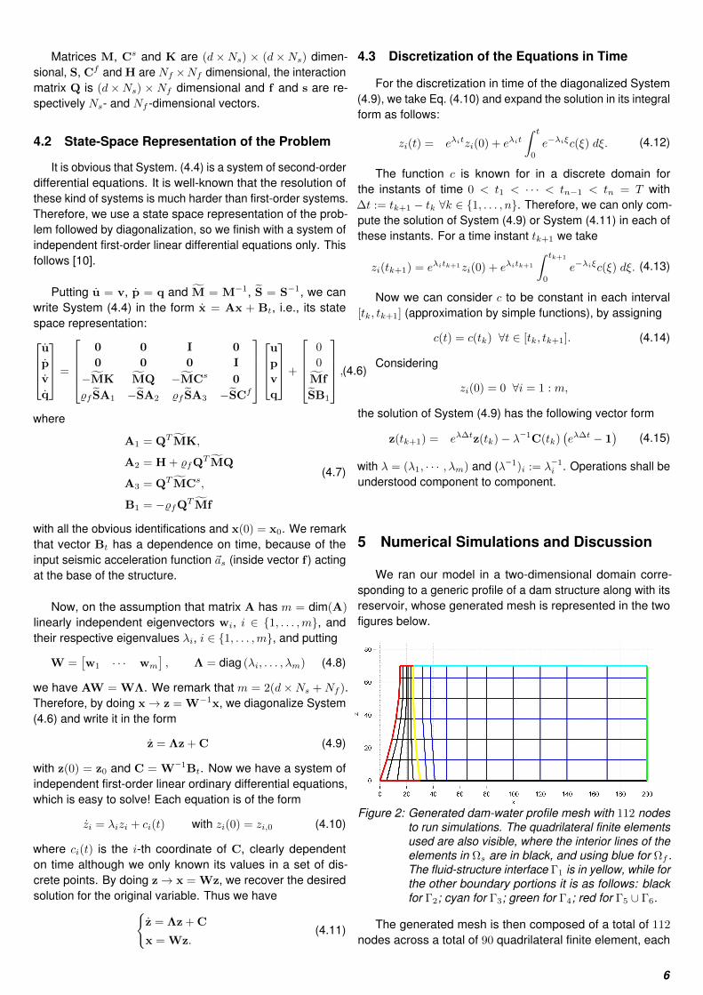
Figure 2: Generated dam-water profile mesh with 112 nodesto run simulations. The quadrilateral finite elementsused are also visible, where the interior lines of theelements in Ωs are in black, and using blue for Ωf .The fluid-structure interface Γ1 is in yellow, while forthe other boundary portions it is as follows: blackfor Γ2; cyan for Γ3; green for Γ4; red for Γ5 ∪ Γ6.

The generated mesh is then composed of a total of 112

nodes across a total of 90 quadrilateral finite element, each

6

touching 4 nodes. A third of the elements are within Ωs (struc-ture elements) and the other 60 are within Ωf (fluid elements),spanning the nodes as follows: 35 nodes are pure structurenodes; 70 nodes are pure fluid node; the rest 7 (the nodeson Γ1) are fluid-structure interaction nodes, i.e., they are both.

The dam composition material is taken as reinforcedconcrete interacting with water with the following materialcharacteristics:

DampingMaterial E(kPa) ν wg(kN/m

3) α β

Concrete 25× 106 0.2 24 0.4 8× 10−6

Water 15× 106 0.2 10 0.5 2× 105

Table 1: Characteristics of the structure reinforced concretematerial and the water in the reservoir.

Also, we take ~g = (0,−9.81), with g = 9.81m/s2, whichimplies %s ≈ 2.44 and %f ≈ 1.02.

Important to remark are the units in which the displace-ment ~u and pressure p variables were modelled in the equa-tions. We used standard units, i.e., meters (m) for the ~u andPascal (Pa) for p.

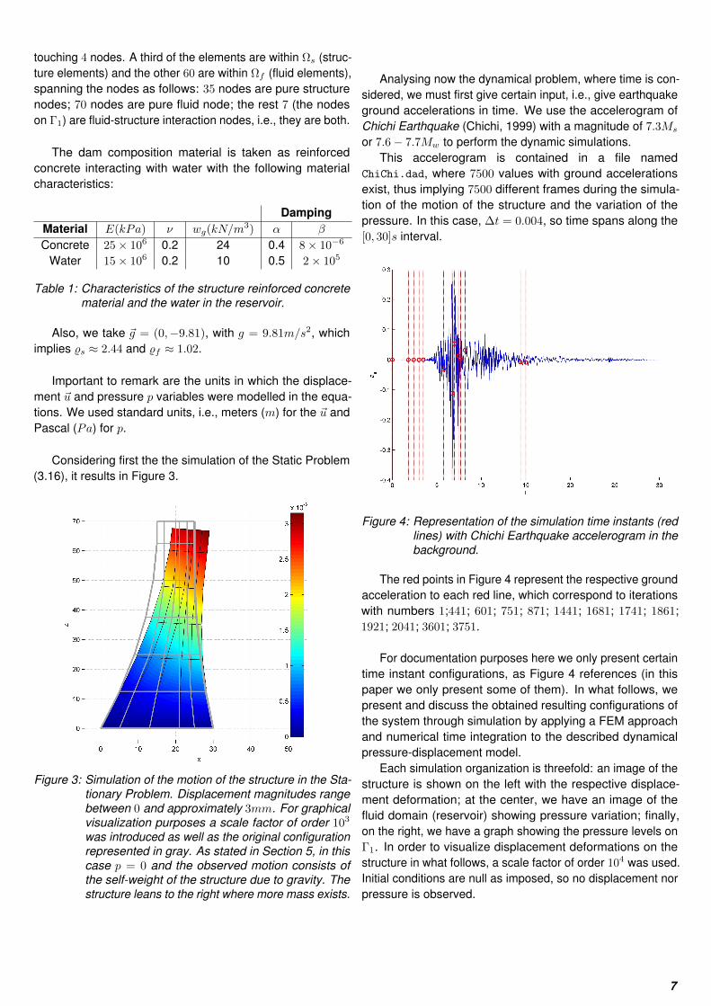
Considering first the the simulation of the Static Problem(3.16), it results in Figure 3.

Figure 3: Simulation of the motion of the structure in the Sta-tionary Problem. Displacement magnitudes rangebetween 0 and approximately 3mm. For graphicalvisualization purposes a scale factor of order 103

was introduced as well as the original configurationrepresented in gray. As stated in Section 5, in thiscase p = 0 and the observed motion consists ofthe self-weight of the structure due to gravity. Thestructure leans to the right where more mass exists.

Analysing now the dynamical problem, where time is con-sidered, we must first give certain input, i.e., give earthquakeground accelerations in time. We use the accelerogram ofChichi Earthquake (Chichi, 1999) with a magnitude of 7.3Ms

or 7.6− 7.7Mw to perform the dynamic simulations.This accelerogram is contained in a file named

ChiChi.dad, where 7500 values with ground accelerationsexist, thus implying 7500 different frames during the simula-tion of the motion of the structure and the variation of thepressure. In this case, ∆t = 0.004, so time spans along the[0, 30]s interval.

Figure 4: Representation of the simulation time instants (redlines) with Chichi Earthquake accelerogram in thebackground.

The red points in Figure 4 represent the respective groundacceleration to each red line, which correspond to iterationswith numbers 1;441; 601; 751; 871; 1441; 1681; 1741; 1861;1921; 2041; 3601; 3751.

For documentation purposes here we only present certaintime instant configurations, as Figure 4 references (in thispaper we only present some of them). In what follows, wepresent and discuss the obtained resulting configurations ofthe system through simulation by applying a FEM approachand numerical time integration to the described dynamicalpressure-displacement model.

Each simulation organization is threefold: an image of thestructure is shown on the left with the respective displace-ment deformation; at the center, we have an image of thefluid domain (reservoir) showing pressure variation; finally,on the right, we have a graph showing the pressure levels onΓ1. In order to visualize displacement deformations on thestructure in what follows, a scale factor of order 104 was used.Initial conditions are null as imposed, so no displacement norpressure is observed.

7

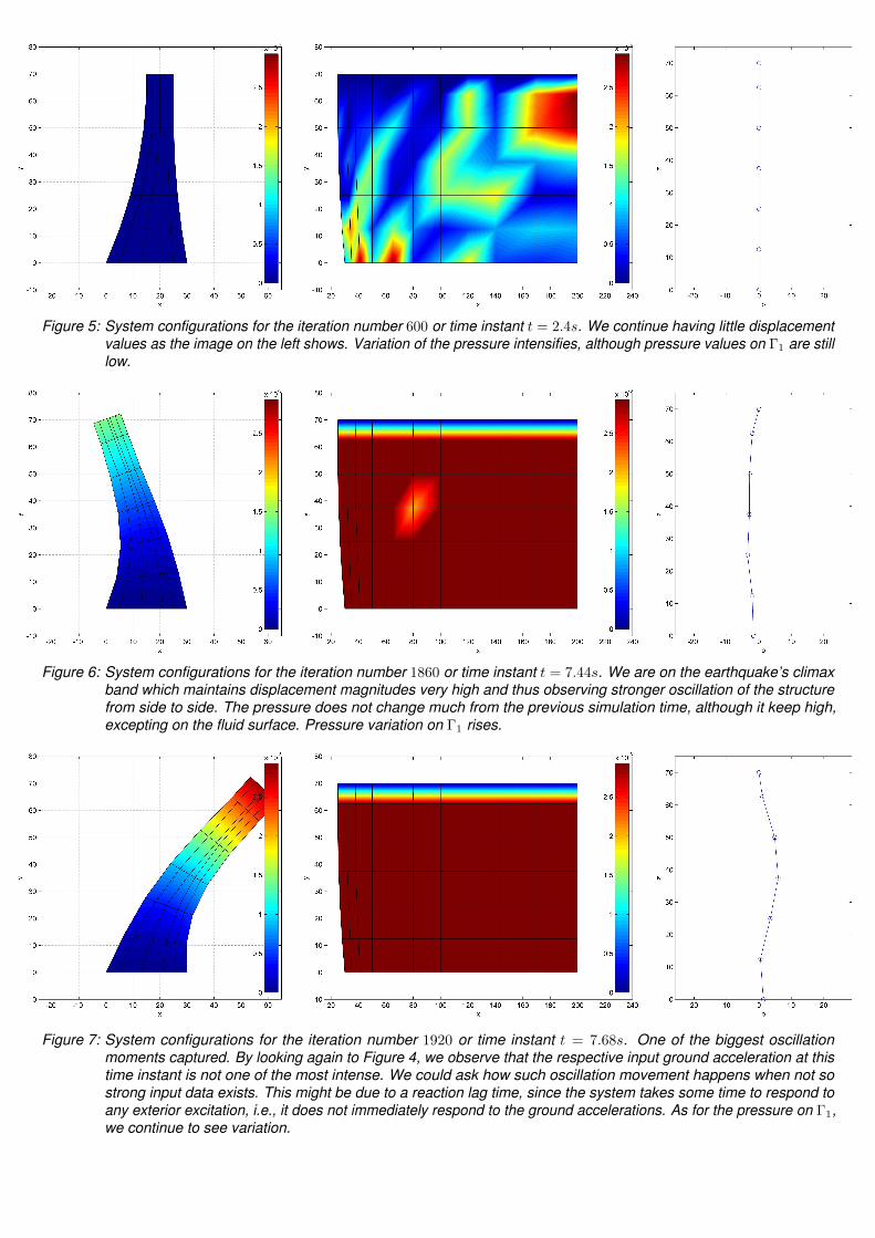
Figure 5: System configurations for the iteration number 600 or time instant t = 2.4s. We continue having little displacementvalues as the image on the left shows. Variation of the pressure intensifies, although pressure values on Γ1 are stilllow.

Figure 6: System configurations for the iteration number 1860 or time instant t = 7.44s. We are on the earthquake’s climaxband which maintains displacement magnitudes very high and thus observing stronger oscillation of the structurefrom side to side. The pressure does not change much from the previous simulation time, although it keep high,excepting on the fluid surface. Pressure variation on Γ1 rises.

Figure 7: System configurations for the iteration number 1920 or time instant t = 7.68s. One of the biggest oscillationmoments captured. By looking again to Figure 4, we observe that the respective input ground acceleration at thistime instant is not one of the most intense. We could ask how such oscillation movement happens when not sostrong input data exists. This might be due to a reaction lag time, since the system takes some time to respond toany exterior excitation, i.e., it does not immediately respond to the ground accelerations. As for the pressure on Γ1,we continue to see variation.

8

Figure 8: System configurations for the iteration number 3750 or time instant t = 15s. The magnitude of the observedstructure displacements decreases greatly. Again, pressure values remain high throughout the whole domain, alsoincluding variation on Γ1.

We analysed several system configurations in the rangeof the first 15 seconds of seismic activity (although only fourare presented here). From this, we shall remark the followingaspects:

• the system seems to have some reaction lag timeresponse to the input data, mainly observed by thevariation of the displacement variable magnitudes;• pressure variation starts immediately with low values

until heavy earthquake activity is felt. When it occursthe obtained structure displacements become quiteevident (visible motion) as well as there exists a pres-sure increase, which coherent with the interactionmodel;• after heavy earthquake activity, although it is visi-

ble that displacement of the structure decreases, it

seems that pressure values keep high. We mustrecall that a fluid behaves quite in a different waywith motion. One excited, a fluid takes considerablymore time to return to rest, which has to do with itsproperties, namely the viscosity (the water is indeedinviscid).

Now we just show a graph comparison between this modeland an alternative structure-structure displacement model.We define the uppermost-right node (a structure node) as acontrol node, where we would constantly check if the com-putational implementation was working or not, and analysethe displacement graphs in the x-axis. We take this node,because it consists of one of the nodes that suffers greaterdeformations.

Figure 9: Displacement deformation on the control node along the x-axis in time for both models: on the left through thepressure-structure interaction model; on the right through the structure-structure model. One cannot say that thegraphs match completely, but they are quite identical following the shape of the introduced accelerogram. Plus,values are in the order of 10−3 for both models.

9

Finally, some discussion on the computational costs mustbe made, since it was observed that computational computingtime was slightly improved.

This is due to the fact that the pressure-displacementmodel has a state space representation with fewer ordinarydifferential equations to be solved. The advantage of takingthe pressure in the fluid nodes is that in this manner we onlyconsider scalar functions. Thus the smaller system. In con-trast, a state space representation of the structure-structuremodel quickly escalates in dimension for the reason that itconsiders vectorial functions for all nodes of the mesh.

In this case, we had a system of 322 equations and vari-ables, while in the correspondent SSM it was 448 equationsand variables. This illustrates that even in this small two-dimensional geometry a significant reduction (roughly a quar-ter of the equations) of the system’s dimension was accom-plished. Thus we leave as suggestion using it for simulationsin 3-D geometries, where more expressive dimension reduc-tion might be obtained.

5.1 Achievements and Future Work

In this dissertation we derived a compressible fluid-flexiblestructure model in a pressure-displacement formulation fromEuler and Navier equations. Some assumptions and approxi-mations were taken to obtain a coupled system of equationsfor the problem. Also the mathematical modelling of physicalphenomena incorporated into the model, namely the undula-tion on the free surface and the radiation boundary, made itmore realistic than an alternative structure-structure model.We then used classical mathematical results and methods inthe field of Functional Analysis and Partial Differential Equa-tions to derived the variational formulation of the problem.

From here, it was possible to see the difficulty of theequations of the model because of the imposed boundaryconditions as well as the interface conditions. This was some-thing not expected at the beginning, since the model is notcompletely unintuitive. Nevertheless, energy estimates forthe solutions were still obtained. Next, we started the dis-cretization of the domain and the equations in space to applyGalerkin’s Finite Element Method followed by a discretizationin time and simulation.

One of the relevant attainments of this paper was theimplementation from scratch of the computational numericalmethod to solve our problem. The awareness about all theproblem’s detailed really was improved. We believe this im-plementation was very successful judging by the simulationsthat we got, and therefore also very useful in future work.

As future research, we think questions like the study ofstability of the equations and possibly some results about ex-istence and uniqueness of solution for the dynamical problemwould be of great interest, for instance by trying to follow theapproach used in [3]. Having this work as some basis, wewould also take now simulations in 3-D domains with realdata and for different kinds of accelerograms, in addition topossibly performing comparisons between obtained valuesand real data measurements for the water pressure.

References

[1] O. C. ZIENKIEWICZ, R. L. TAYLOR, J. Z. ZHU, (2006)18 Coupled Systems in O. C. ZIENKIEWICZ, R. L. TAY-LOR, J. Z. ZHU, The Finite Element Method: Its Basis& Fundamentals, Sixth Edition, Elsevier Butterworth-Heinemann,

[2] LAWRENCE C. EVANS, (2010) Partial Differential Equa-tions, Graduate Studies in Mathematics, Second Edition,American Mathematical Society Press

[3] C. HSIAO, George, SAYAS, Francisco-Javier, J.WAINACHT, Richard, (2014) Time-Dependent Fluid-Structure Interaction, University of DelawareRetrieved by the code USAarXiv:1406.2171v1

[4] G. P. GALDI, (2011), An Introduction to the Mathemat-ical Theory of the Navier-Stokes Equations. Steady-State Problems, Second Edition, Springer Monographsin Mathematics

[5] HAIM BREZIS, (2011), Sobolev Spaces and the Vari-ational Formulation of Boundary Value Problems inOne Dimension in HAIM BREZIS, Functional Analysis,Sobolev Spaces and Partial Differential Equations, FirstEdition, Springer

[6] WILLIAM LAYTON, (2008) Introduction to the NumericalAnalysis of Incompressible Viscous Flows, SIAM

[7] B. Tiliouine & A. Seghir, Fluid-structure models for Dy-namic Studies of dam-water systems, École NationalePolytechnique, Algiers, Retrieved fromhttp://www.freewebs.com/seghir/pubs/ecee98.pdf

[8] SELLIER Damien, FOURCAUD Therry, LAC, Patrick,(2006), A finite element model for investigating effects ofaerial architecture on tree oscillations, Tree Physiology,vol. 26, pp. 799?806

[9] KASELOW, Axel, (2004), The Stress Sensitivity Ap-proach: Theory and Application, [Dissertation for Doctorin Geophysics], Freie Universität BerlinRetrieved from FUDISS_derivate_000000001276

[10] ROWELL, Derek, (2002), Time-Domain Solution of LTIState Equations, [Lectures Notes for the course in Anal-ysis and Design of Feedback Control Systems], MIT

[11] OLIVEIRA, Sergio, (2001), Mecânica dos Sólidos III,Dos Fundamentos às Aplicações: Equações fundamen-tais da Mecânica dos Sólidos e desenvolvimento de pro-gramas para cálculo de estruturas 2D e 3D pelo Métododos Elementos Finitos, [Lecture Notes for the Master inCivil Engineering], Instituto Superior de Engenharia deLisboa

[12] T. SANDWELL, David, (2009), Brief Review of Elas-ticity, [Lecture Notes for the course in Geodynamics],University of California San Diego

[13] LAMOUREUX, Michael P., (2006) The mathematics ofPDEs and the wave equation, [Lecture Notes for SeismicImaging Summer School], University of Calgary

10