Fluid structure interaction in flexible vessels
208
Fluid structure interaction in flexible vessels Christina Grigoria Giannopapa Thesis submitted for the Degree of Doctor of Philosophy of the University of London King’s College London 2004
Transcript of Fluid structure interaction in flexible vessels

Fluid structure interaction in flexible
vessels
Christina Grigoria Giannopapa
Thesis submitted for the
Degree of Doctor of Philosophy of the University of London
King’s College London
2004

Dedicated to my grandmother Mrs Christina Katrivanou,
to my parents and to my cousin George.
SUPERVISORS
Dr. G. Papadakis
Dr. M.C.M Rutten (Eindhoven University of Technology)
Dr. K. Lee
Copyright c© 2004 by Christina G. Giannopapa
All rights are reserved. No part of this publication may be reproduced, stored in re-
trieval system, or transmitted, in any form or by any means, electronic, mechanical,
photocopying, recording or otherwise, without prior permission of the author.
This research was conducted in King’s College London (UK) and in Eindhoven
University of Technology (The Netherlands). Financially support was provided by
EPSRC, King’s College London and Marie Curie Fellowships, European Commis-
sion.

Abstract
The thesis is concerned with the study of fluid-structure interaction in flexible tubes
both from the modelling as well as the experimental point of view.
More specifically, it presents the first stage of development and testing of a novel
unified solution method suitable for fluid-structure interaction problems. In the
conventional approach for modelling such problems, the fluid and solid components
are treated separately, information is exchanged at their interface and different so-
lution algorithms are used for the two components. The equations for solids are
solved for displacement and stress and, the ones for fluids are solved for velocity and
pressure. The exchange of information between two solution methods that solve for
different quantities is not a trivial task and has also known drawbacks such as high
computational cost and potential numerical instabilities, especially for very flexible
structures. In the new method presented in the thesis, a single set of equations is
used to describe both fluid and solid, while the interface between them is contained
within the solution domain itself. This is achieved by reformulating the solid equa-
tions to contain the same primitive variables used in fluids i.e. velocity and pressure.
The PISO algorithm is used to handle the velocity-pressure coupling. The method
proposed is fully tested for solids on a structural dynamic problem (beam bending)
and the results compared successfully with the classical structural analysis. In order
to quantify the dissipation characteristics of the numerical integration technique, a
stability eigenvalue analysis of the proposed time marching and spatial discretisation
scheme is performed in one dimension but the conclusions of this analysis were also
in agreement with the results of the beam bending.
The new formulation for solids is found to be stable and robust, thus it can be
used in the next stage of testing in full fluid-structure-interaction problems. The
new algorithm can be validated against the results obtained during the experimental
phase of the work, which is focused on wave propagation in flexible vessels. This
experimental study is also motivated by the need to understand arterial blood flow.
Although the general principles governing the arterial hemodynamics are well known,
the assessment of non-linearities arising from wall thickness variation and geometric
tapering, naturally present in the arterial tree morphology, have not been fully
investigated. To this end, a complete experimental data set on wave propagation was
collected for six flexible tubes with different wall thickness and geometric tapering.
i

ii
A special manufacturing methodology was used to produce the tubes. They were
manufactured in such a way that pairs of tubes had the same wave speed according to
the linear pulse wave propagation theory. Any discrepancy in the wave propagation
characteristics thus indicates the importance of the non-linearities. The measured
quantities were pressure and pressure gradient using two pressure wires, flow rate
using a ultrasound flow probe, and wall distension using ultrasound. The geometric
tapering was found to be of great importance as it alters the shape of the pressure
signal. The experimental measurements of the straight tubes are compared with
the linear theory and highly encouraging levels of agreement are found when the
viscoelastic properties of the wall are taken into account.

Acknowledgements
I would like to express my sincere gratitude to my supervisors: Dr. G. Papadakis,
Dr. M.C.M. Rutten (Eindhoven University of Technology) and Dr. K.C. Lee, for
their continuous interest, support and guidance during this study. Equally I would
like to thank Dr. A.S. Tijsseling (Eindhoven University of Technology) who has
been my supervisor under the European Commission Marie Curie Fellowship grant.
I am indebted to my colleagues and friends in the groups of Prof. M. Yianneskis,
Prof. R.M.M. Mattheij (Eindhoven University of Technology) and Prof. F.N. van de
Vosse (Eindhoven University of Technology), as well as the Professors themselves.
In particular I would like to thank Dr. M.E. Verbeek (Eindhoven University of
Technology) for his numerous valuable comments.
I am grateful to Mr. M.W. Wijlaars (Eindhoven University of Technology) for
his help and guidance in the laboratory, Mrs E.R.H. van Dijk (Eindhoven University
of Technology) and Mr. J. Greenberg for the arrangement of many administrative
matters.
I would like to thank Dr. C.J. Greenshields for helping me during the first year
to aquire the background knowledge needed to develop the unified solution method
and for initially stimulating my interest in the field; and Mr. H. Weller from Nabla
Ltd. for his initial assistance on technical issues related to the finite volume C++
library.
I am sincerely greatful to Dr. S. Balabani for being my guardian angel during
my entire studies in King’s College London; I am in debt to her for life.
Finally, I would like to thank Mr. J.D. Malo and Mr. R.J. Smits from Research
DG, European Commission for allowing me to allocate time in writing up this thesis
while working for them. I would also like to thank Mr. G. Papageorgiou and Mr.
P. Keraudren for their advice and support in related administrative maters.
The financial support provided by the EPSRC (Engineering and Physical Sci-
ences Research Council) under the GR/N65769 grant, by the King’s College London
top up grant and by the Marie Curie Fellowships supported by the European Com-
mission is greatfully acknowledged.
iii

iv Contents

Contents
Contents iv
List of Figures ix
List of Tables xv
Nomenclature xvi
1 Introduction and literature survey 1
1.1 General Introduction . . . . . . . . . . . . . . . . . . . . . . . . . . . 1
1.2 Morphology of arteries . . . . . . . . . . . . . . . . . . . . . . . . . . 2
1.2.1 Wall layers . . . . . . . . . . . . . . . . . . . . . . . . . . . . . 3
1.2.2 Wall dimensions . . . . . . . . . . . . . . . . . . . . . . . . . . 4
1.3 Computational Methods for fluid structure interaction . . . . . . . . 4
1.4 Wave propagation in flexible vessels . . . . . . . . . . . . . . . . . . . 10
1.4.1 Theoretical models on straight tubes . . . . . . . . . . . . . . 10
1.4.2 Experimental models on straight tubes . . . . . . . . . . . . . 13
1.4.3 Theoretical models on tapered tubes . . . . . . . . . . . . . . 16
1.4.4 Experimental models on tapered tubes . . . . . . . . . . . . . 17
1.4.5 Concluding summary . . . . . . . . . . . . . . . . . . . . . . . 18
1.5 Objectives of this study . . . . . . . . . . . . . . . . . . . . . . . . . 21
1.6 Outline of the thesis . . . . . . . . . . . . . . . . . . . . . . . . . . . 23
2 Mathematical formulation of a unified framework for fluids and
solids 25
2.1 Introduction . . . . . . . . . . . . . . . . . . . . . . . . . . . . . . . . 25
2.2 Governing Equations . . . . . . . . . . . . . . . . . . . . . . . . . . . 25
2.3 Mathematical Model . . . . . . . . . . . . . . . . . . . . . . . . . . . 27
2.3.1 Standard stress analysis for linear elastic (or Hookean) solid . 28
2.3.2 Velocity based formulation for linear elastic (or Hookean) solid 28
2.3.3 Velocity and Pressure based formulation for linear elastic (or
Hookean) solid . . . . . . . . . . . . . . . . . . . . . . . . . . 29
v
vi Contents
2.4 Comparison of the new velocity-pressure formulation for solids with
the fluids formulation . . . . . . . . . . . . . . . . . . . . . . . . . . . 31
2.5 Boundary conditions . . . . . . . . . . . . . . . . . . . . . . . . . . . 32
2.6 Closure . . . . . . . . . . . . . . . . . . . . . . . . . . . . . . . . . . . 33
3 Numerical solution method 35
3.1 Introduction . . . . . . . . . . . . . . . . . . . . . . . . . . . . . . . 35
3.2 Discretisation Procedure . . . . . . . . . . . . . . . . . . . . . . . . . 37
3.2.1 Determination the face value φ f . . . . . . . . . . . . . . . . . 39
3.2.2 Discretisation of the gradient . . . . . . . . . . . . . . . . . . 40
3.2.3 Discretisation of the divergence . . . . . . . . . . . . . . . . . 41
3.2.4 Discretisation of the Laplacian term . . . . . . . . . . . . . . 41
3.2.5 Laplacian versus Divergence-Grad . . . . . . . . . . . . . . . 41
3.2.6 Temporal Discretisation . . . . . . . . . . . . . . . . . . . . . 43
3.2.7 Boundary Conditions . . . . . . . . . . . . . . . . . . . . . . . 46
3.3 Final form of equations and discretisation of the transient term . . . 48
3.3.1 Reformulation in order to increase convergence rate . . . . . . 48
3.3.2 Temporal discretisation approaches . . . . . . . . . . . . . . . 49
3.4 Iterative solution methods of governing equations . . . . . . . . . . . 52
3.4.1 Governing equations . . . . . . . . . . . . . . . . . . . . . . . 52
3.4.2 Non-linearity and pressure/velocity coupling . . . . . . . . . . 53
3.4.3 Derivation of pressure equation . . . . . . . . . . . . . . . . . 54
3.4.4 Velocity-Pressure coupling algorithms . . . . . . . . . . . . . . 56
3.5 Investigation of boundary conditions for fluids . . . . . . . . . . . . . 59
3.6 Boundary condition for solids for the unified solution method . . . . 63
3.6.1 Boundary conditions for the displacement formulation . . . . . 64
3.6.2 Boundary conditions for the velocity formulation . . . . . . . 64
3.6.3 Boundary conditions for the velocity-pressure formulation . . . 65
3.6.3.1 Boundary conditions for velocity . . . . . . . . . . . 65
3.6.3.2 Boundary condition types for pressure . . . . . . . . 66
3.6.4 Optimal choice of boundary conditions . . . . . . . . . . . . . 67
3.7 Stability Analysis . . . . . . . . . . . . . . . . . . . . . . . . . . . . . 68
3.7.1 Wave equation (1D) . . . . . . . . . . . . . . . . . . . . . . . 70
3.7.2 Velocity formulation for linear elastic Hookean solid (1D) . . . 72
3.8 Closure . . . . . . . . . . . . . . . . . . . . . . . . . . . . . . . . . . . 78
4 Validation of the new formulation for solids 81
4.1 Introduction . . . . . . . . . . . . . . . . . . . . . . . . . . . . . . . . 81
4.2 Case Description . . . . . . . . . . . . . . . . . . . . . . . . . . . . . 81
4.3 Analytical solution . . . . . . . . . . . . . . . . . . . . . . . . . . . . 82
4.4 Results . . . . . . . . . . . . . . . . . . . . . . . . . . . . . . . . . . . 85

Contents vii
4.4.1 Displacement calculated using the standard stress analysis . . 85
4.4.2 Discretisation error analysis for the new formulations . . . . . 87
4.4.2.1 Calculation of the accumulated term . . . . . . . . . 88
4.4.2.2 Temporal term discretisation . . . . . . . . . . . . . 91
4.4.2.3 Mesh quality . . . . . . . . . . . . . . . . . . . . . . 96
4.4.3 Boundary conditions . . . . . . . . . . . . . . . . . . . . . . . 97
4.4.4 Other cases . . . . . . . . . . . . . . . . . . . . . . . . . . . . 98
4.4.4.1 Analytical solution . . . . . . . . . . . . . . . . . . 98
4.4.4.2 Numerical solution . . . . . . . . . . . . . . . . . . . 98
4.5 Closure . . . . . . . . . . . . . . . . . . . . . . . . . . . . . . . . . . . 100
5 Wave propagation experiments in flexible vessels with wall thick-
ness variation and geometric tapering 105
5.1 Introduction . . . . . . . . . . . . . . . . . . . . . . . . . . . . . . . . 105
5.2 The Tube Models Methodology . . . . . . . . . . . . . . . . . . . . . 105
5.2.1 The vessels design and specifications . . . . . . . . . . . . . . 106
5.2.2 Manufacturing Method . . . . . . . . . . . . . . . . . . . . . . 109
5.3 Material Properties of the Tubes . . . . . . . . . . . . . . . . . . . . 109
5.4 Measurement Methods . . . . . . . . . . . . . . . . . . . . . . . . . . 112
5.4.1 Experimental set-up . . . . . . . . . . . . . . . . . . . . . . . 112
5.4.2 Instrumentation . . . . . . . . . . . . . . . . . . . . . . . . . . 113
5.4.3 Protocol . . . . . . . . . . . . . . . . . . . . . . . . . . . . . . 114
5.4.4 Data processing . . . . . . . . . . . . . . . . . . . . . . . . . . 115
5.5 Results . . . . . . . . . . . . . . . . . . . . . . . . . . . . . . . . . . . 115
5.5.1 Static pressure - initial diameter relation . . . . . . . . . . . . 115
5.5.2 Standard deviation of measurements . . . . . . . . . . . . . . 117
5.5.3 Fluid motion . . . . . . . . . . . . . . . . . . . . . . . . . . . 117
5.5.4 Wall motion . . . . . . . . . . . . . . . . . . . . . . . . . . . . 127
5.6 Closure . . . . . . . . . . . . . . . . . . . . . . . . . . . . . . . . . . . 136
6 Comparison of experimental results with linear wave propagation
methods 137
6.1 Introduction . . . . . . . . . . . . . . . . . . . . . . . . . . . . . . . . 137
6.2 Linear Theory of Wave Propagation in Flexible Vessels . . . . . . . . 137
6.2.1 Basic theory . . . . . . . . . . . . . . . . . . . . . . . . . . . . 138
6.2.2 Wave propagation speeds . . . . . . . . . . . . . . . . . . . . . 140
6.2.3 Wave reflections through discrete transitions . . . . . . . . . . 142
6.3 Implementation of the continuous linear model . . . . . . . . . . . . . 144
6.4 Comparisons with Linear Model for Elastic Material . . . . . . . . . . 144
6.5 Comparisons with Linear Model for Viscoelastic Material . . . . . . . 145
6.6 Closure . . . . . . . . . . . . . . . . . . . . . . . . . . . . . . . . . . . 145

viii Contents
7 Conclusions 159
7.1 Overview . . . . . . . . . . . . . . . . . . . . . . . . . . . . . . . . . 159
7.2 Main achievements . . . . . . . . . . . . . . . . . . . . . . . . . . . . 161
7.3 Future work . . . . . . . . . . . . . . . . . . . . . . . . . . . . . . . . 162
7.3.1 Mathematical modelling . . . . . . . . . . . . . . . . . . . . . 162
7.3.2 Experimental work . . . . . . . . . . . . . . . . . . . . . . . . 164
Bibliography 165
A The Tube Models Manufacturing Methodology i
A.1 The vessels design and specifications . . . . . . . . . . . . . . . . . . i
A.2 Manufacturing set-up . . . . . . . . . . . . . . . . . . . . . . . . . . . iii
A.3 Equations for manufacturing . . . . . . . . . . . . . . . . . . . . . . . iii
A.4 Straight tube manufacturing . . . . . . . . . . . . . . . . . . . . . . . v
A.4.1 Constant thickness . . . . . . . . . . . . . . . . . . . . . . . . vi
A.4.2 Variable thickness . . . . . . . . . . . . . . . . . . . . . . . . . vi
A.5 Tapered tube manufacturing . . . . . . . . . . . . . . . . . . . . . . . viii
A.5.1 Constant thickness . . . . . . . . . . . . . . . . . . . . . . . . viii
A.5.2 Variable thickness . . . . . . . . . . . . . . . . . . . . . . . . . xi
A.6 Wall thickness accuracy . . . . . . . . . . . . . . . . . . . . . . . . . xi

List of Figures
1.1 FSI categories. . . . . . . . . . . . . . . . . . . . . . . . . . . . . . . 2
1.2 Cross sections of the arterial wall (not to scale). . . . . . . . . . . . . 3
1.3 Solution procedure of several FSI methods. . . . . . . . . . . . . . . . 6
1.4 FSI methods conventional terminology. . . . . . . . . . . . . . . . . . 7
2.1 The velocity integral from [t0, t +∆t] . . . . . . . . . . . . . . . . . . . 28
3.1 Cell based structure. . . . . . . . . . . . . . . . . . . . . . . . . . . . 38
3.2 Evaluation of the face value φ f from cell centre values φP and φN
assuming linear interpolation. . . . . . . . . . . . . . . . . . . . . . . 40
3.3 Cells involved in the evaluation of the Laplacian operator at cell with
cell centre denoted as P. . . . . . . . . . . . . . . . . . . . . . . . . . 42
3.4 Cells involved in the evaluation of the Divergence- Gradient operator
at cell with centre denoted as P. . . . . . . . . . . . . . . . . . . . . . 43
3.5 PISO algorithm flow chart for compressible flow (for one time step). . 57
3.6 Shortest resolvable wave. . . . . . . . . . . . . . . . . . . . . . . . . . 68
3.7 Stencil for the 1D hyperbolic finite difference equation (3.90). . . . . 70
3.8 Accuracy portrait of the amplification factor G for the 1D hyperbolic
equation (3.96). . . . . . . . . . . . . . . . . . . . . . . . . . . . . . . 73
3.9 Stencil for the 1D system of equations that is equivalent to the 1D
velocity formulation. . . . . . . . . . . . . . . . . . . . . . . . . . . . 75
3.10 Amplitude portrait of the 1D velocity formulation in comparison with
the wave equation (displacement formulation). . . . . . . . . . . . . . 77
4.1 Beam bending test case. . . . . . . . . . . . . . . . . . . . . . . . . . 82
4.2 Analytical calculations for the vibration eigenvalues, eigenmodes and
frequency of oscilation using a 1D approximation for the solution of
a cantilever beam. . . . . . . . . . . . . . . . . . . . . . . . . . . . . . 84
4.3 End displacement (m) versus time (s) (standard stress analysis). . . . 86
4.4 Standard stress analysis (envelope of displacement). . . . . . . . . . . 87
4.5 Total power comparison for the ∇2 and the ∇ •∇ operators in the
accumulated term. . . . . . . . . . . . . . . . . . . . . . . . . . . . . 90
4.6 Total power comparison for different tolerances:10e-6, 10e-7, 10e-8. . . 91
ix
x List of Figures
4.7 Comparison of displacement formulation and velocity-based formula-
tion for the Euler Implicit discretisation scheme (envelope of displace-
ment). . . . . . . . . . . . . . . . . . . . . . . . . . . . . . . . . . . 92
4.8 Comparison of Euler Implicit and Backward Differencing discretisa-
tion scheme (envelope of displacement). . . . . . . . . . . . . . . . . . 93
4.9 Comparison of different time step sizes: 1e-4, 1e-5, 1e-6 s for the first
time derivative Euler Implicit. . . . . . . . . . . . . . . . . . . . . . . 94
4.10 Comparison of Euler Implicit using time step size 1e-5 s against Back-
ward differencing using time step size of 1e-4 s (envelope of displace-
ment). . . . . . . . . . . . . . . . . . . . . . . . . . . . . . . . . . . . 95
4.11 Mesh resolution comparison for meshes: 40x10, 60x20 and 200x50
cells. Time step size used is 1e-4 and temporal term discretisation
scheme is Backward differencing (envelope of displacement). . . . . . 96
4.12 Comparison of different boundary conditions for pressure in the fully
implicit velocity-pressure formulation. . . . . . . . . . . . . . . . . . . 97
4.13 Beam with size 10mx5m. No of cells used for the mesh is 20x10cells
, time step size used is 1e-4 and temporal term discretisation scheme
is Backward differencing. . . . . . . . . . . . . . . . . . . . . . . . . . 99
4.14 Beam with size 40mx5m. No of cells used for the mesh is 80x10cells ,
time step size used is 1e-4 s and temporal term discretisation scheme
is Backward differencing. . . . . . . . . . . . . . . . . . . . . . . . . . 100
4.15 Beam with size 20mx5m, with applied end shear τ = 5e5Pa. No of
cells used for the mesh is 40x10cells , time step size used is 1e-4 s and
temporal term discretisation scheme is Backward differencing. . . . . 101
5.1 Wall thickness variation for tubes C and F. . . . . . . . . . . . . . . . 108
5.2 Typical relaxation test curve for Polyurethane specimen (3% elonga-
tion). . . . . . . . . . . . . . . . . . . . . . . . . . . . . . . . . . . . . 110
5.3 Experimental set-up for wave propagation experiments (TU/e). . . . 113
5.4 Static pressure-initial diameter relation of the straight tube (Type B). 116
5.5 A typical result at a location showing the mean of 16 measurements
and the standard deviation from the mean. . . . . . . . . . . . . . . 117
5.6 Normalised pressure measurements every 50 mm along the length
of the tube against scaled time for straight tubes: types A,B,C (A:
straight tube with constant wall thickness of 0.1 mm; B: straight
tube with constant wall thickness of 0.05 mm; C: straight tube with
variable wall thickness of 0.05-0.1 mm). . . . . . . . . . . . . . . . . . 118

List of Figures xi
5.7 Normalised pressure measurements every 50 mm along the length of
the tube against time for tapered tubes: types D,E,F (D: tapered
tube with constant wall thickness of 0.1 mm; E: tapered tube with
constant wall thickness of 0.05 mm; F:tapered tube with variable wall
thickness of 0.1-0.05 mm). . . . . . . . . . . . . . . . . . . . . . . . . 119
5.8 Normalised pressure measurements every 50 mm along the length of
the tube against time for tube types A and F (A: straight tube with
constant wall thickness of 0.1 mm; F: tapered tube with variable wall
thickness of 0.1-0.05 mm). . . . . . . . . . . . . . . . . . . . . . . . . 120
5.9 Normalised pressure measurements every 50 mm along the length of
the tube against time for tubes types C and E (C: straight tube with
variable wall thickness 0.05-0.1 mm; E: tapered tube with constant
wall thickness of 0.05 mm). . . . . . . . . . . . . . . . . . . . . . . . 121
5.10 Normalised flow rate measurements every 50 mm along the length
of the tube against scaled time for straight tubes: types A, B, C
(A: straight tube with constant wall thickness of 0.1 mm; B: straight
tube with constant wall thickness of 0.05 mm; C: straight tube with
variable wall thickness of 0.05-0.1 mm). . . . . . . . . . . . . . . . . . 123
5.11 Normalised flow rate measurements every 50 mm along the length
of the tube against scaled time for straight tubes: types D, E, F
(D: tapered tube with constant wall thickness of 0.1 mm; E: tapered
tube with constant wall thickness of 0.05 mm; F: tapered tube with
variable wall thickness of 0.1-0.05 mm). . . . . . . . . . . . . . . . . . 124
5.12 Normalised flow rate measurements every 50 mm along the length of
the tube against time for tubes types A and F (A: straight tube with
constant wall thickness of 0.1 mm; F: tapered tube with variable wall
thickness of 0.1-0.05 mm). . . . . . . . . . . . . . . . . . . . . . . . . 125
5.13 Normalised flow rate measurements every 50 mm along the length of
the tube against time for tubes types C and E (C: straight tube with
variable wall thickness 0.05-0.1 mm; E: tapered tube with constant
wall thickness of 0.05 mm). . . . . . . . . . . . . . . . . . . . . . . . 126
5.14 Normalised pressure gradient measurements every 50 mm along the
length of the tube against time for tubes types A, B, C (A: straight
tube with constant wall thickness of 0.1 mm; B: straight tube with
constant wall thickness of 0.05 mm; C: straight tube with variable
wall thickness of 0.05-0.1 mm). . . . . . . . . . . . . . . . . . . . . . 128

xii List of Figures
5.15 Normalised pressure gradient measurements every 50 mm along the
length of the tube against time for tubes types D, E, F (D: tapered
tube with constant wall thickness of 0.1 mm; E: tapered tube with
constant wall thickness of 0.05 mm; F: tapered tube with variable
wall thickness of 0.1-0.05 mm). . . . . . . . . . . . . . . . . . . . . . 129
5.16 Normalised pressure gradient measurements every 50 mm along the
length of the tube against time for tubes types A and F (A: straight
tube with constant wall thickness of 0.1 mm; F: tapered tube with
variable wall thickness of 0.1-0.05 mm). . . . . . . . . . . . . . . . . . 130
5.17 Normalised pressure gradient measurements every 50 mm along the
length of the tube against time for tubes types C and E (C: straight
tube with variable wall thickness 0.05-0.1 mm; E: tapered tube with
constant wall thickness of 0.05 mm). . . . . . . . . . . . . . . . . . . 131
5.18 Normalised wall motion measurements every 50 mm along the length
of the tube against time for tubes types A, B, C (A: straight tube with
constant wall thickness of 0.1 mm; B: straight tube with constant wall
thickness of 0.05 mm; C: straight tube with variable wall thickness of
0.05-0.1 mm). . . . . . . . . . . . . . . . . . . . . . . . . . . . . . . . 132
5.19 Normalised wall motion measurements every 50 mm along the length
of the tube against time for tubes types D, E, F (D: tapered tube with
constant wall thickness of 0.1 mm; E: tapered tube with constant wall
thickness of 0.05 mm; F: tapered tube with variable wall thickness of
0.1-0.05 mm). . . . . . . . . . . . . . . . . . . . . . . . . . . . . . . . 133
5.20 Normalised wall motion measurements every 50 mm along the length
of the tube against time for tubes types A and F (A: straight tube
with constant wall thickness of 0.1 mm; F: tapered tube with variable
wall thickness of 0.1-0.05 mm). . . . . . . . . . . . . . . . . . . . . . 134
5.21 Normalised wall motion measurements every 50 mm along the length
of the tube against time for tubes types C and E (C: straight tube with
variable wall thickness 0.05-0.1 mm; E: tapered tube with constant
wall thickness of 0.05 mm). . . . . . . . . . . . . . . . . . . . . . . . . 135
6.1 Tube motion variables. Point P(z, r) on the surface of the wall at rest
displaces to position P’(z+ζ, r +ξ) . . . . . . . . . . . . . . . . . . . 138
6.2 Discrete transitions between segments. . . . . . . . . . . . . . . . . . 142
6.3 Properties used for the calculations. . . . . . . . . . . . . . . . . . . . 144
6.4 Comparison of pressure experimental measurements of the straight
tube with constant wall thickness of 0.1 mm with linear analytical
model foran elastic tube. . . . . . . . . . . . . . . . . . . . . . . . . . 146

List of Figures xiii
6.5 Comparison of the experimental measurements of the flow on a straight
tube with constant wall thickness of 0.1 mm with linear analytical
model foran elastic tube. . . . . . . . . . . . . . . . . . . . . . . . . . 147
6.6 Comparison of the experimental measurements of the wall distension
on a straight tube with constant wall thickness of 0.1 mmwith linear
analytical model foran elastic tube. . . . . . . . . . . . . . . . . . . . 148
6.7 Comparison of pressure experimental measurements of the straight
tube with constant wall thickness of 0.05 mm with linear analytical
model foran elastic tube. . . . . . . . . . . . . . . . . . . . . . . . . . 149
6.8 Comparison of the experimental measurements of the flow on a straight
tube with constant wall thickness of 0.05 mm with linear analytical
model foran elastic tube. . . . . . . . . . . . . . . . . . . . . . . . . . 150
6.9 Comparison of the experimental measurements of the wall distension
on a straight tube with constant wall thickness of 0.05 mmwith linear
analytical model foran elastic tube. . . . . . . . . . . . . . . . . . . . 151
6.10 Comparison of the experimental measurements of the pressure on
a straight tube with constant wall thickness of 0.1 mm with linear
analytical model fora viscoelastic tube. . . . . . . . . . . . . . . . . . 152
6.11 Comparison of the experimental measurements of the flow on a straight
tube with constant wall thickness of 0.1 mm with linear analytical
model fora viscoelastic tube. . . . . . . . . . . . . . . . . . . . . . . 153
6.12 Comparison of the experimental measurements of the wall distension
on a straight tube with constant wall thickness of 0.1 mmwith linear
analytical model fora viscoelastic tube. . . . . . . . . . . . . . . . . 154
6.13 Comparison of the experimental measurements of the pressure on a
straight tube with constant wall thickness of 0.05 mm with linear
analytical model fora viscoelastic tube. . . . . . . . . . . . . . . . . . 155
6.14 Comparison of the experimental measurements of the flow on a straight
tube with constant wall thickness of 0.05 mm with linear analytical
model fora viscoelastic tube. . . . . . . . . . . . . . . . . . . . . . . 156
6.15 Comparison of the experimental measurements of the wall distension
on a straight tube with constant wall thickness of 0.1 mmwith linear
analytical model fora viscoelastic tube. . . . . . . . . . . . . . . . . 157
7.1 The different properties distribution in the single mesh for solving
fluid structure interaction problems with the unified solution method. 163
A.1 Spin coating set-up ( TU/e). . . . . . . . . . . . . . . . . . . . . . . . iv
A.2 Spin coating process of a tube. . . . . . . . . . . . . . . . . . . . . . . iv
A.3 Straight tube steel rod dimensions. . . . . . . . . . . . . . . . . . . . vi

xiv List of Figures
A.4 Translational velocity, rotational velocity, tube wall thickness and
tube diameter versus the tube length for tube C. . . . . . . . . . . . . vii
A.5 Tapered tube steel rod dimensions. . . . . . . . . . . . . . . . . . . . viii
A.6 Translational velocity, rotational velocity, tube wall thickness and
tube diameter versus the tube length for tube E. . . . . . . . . . . . . x
A.7 Translational velocity, rotational velocity, tube wall thickness and
tube diameter versus the tube length for tube F. . . . . . . . . . . . . xii

List of Tables
1.1 Modelling assumptions for the fluid and solid component as found in
the literature. . . . . . . . . . . . . . . . . . . . . . . . . . . . . . . . 11
1.2 Assumptions for the fluid-solid components for straight tubes as found
in the literature. . . . . . . . . . . . . . . . . . . . . . . . . . . . . . . 19
1.3 Fluid-solid assumptions for tapered tubes as found in the literature. . 20
3.1 Fourier series forms for time level n, n−1, n−2 and grid points j −1,
j, j +1. . . . . . . . . . . . . . . . . . . . . . . . . . . . . . . . . . . 71
4.1 Material properties and dimentions of the beam. . . . . . . . . . . . . 81
4.2 Computational calculations for the vibration eigenfrequencies of vi-
bration using for the two dimensional beam bending case using the
ANSYS finite element commercial package. . . . . . . . . . . . . . . 95
4.3 Comparison between analytical and computational solution for beams
with different size. . . . . . . . . . . . . . . . . . . . . . . . . . . . . 99
5.1 Aorta anatomical data (Westerhof et al., 1969). . . . . . . . . . . . . 106
5.3 Geometrical parameters of tubes manufactured. . . . . . . . . . . . . 107
5.4 Physical properties of polyurethane. . . . . . . . . . . . . . . . . . . . 109
6.1 Values of coefficient ψ describing different longitudinal support con-
ditions for thin- and thick-wall tubes. . . . . . . . . . . . . . . . . . . 141
A.1 Aorta anatomical data (Westerhof et al., 1969). . . . . . . . . . . . . i
A.3 Geometrical parameters of tubes manufactured. . . . . . . . . . . . . ii
A.5 Straight tube specifications. . . . . . . . . . . . . . . . . . . . . . . . v
A.7 Tapered tube specifications. . . . . . . . . . . . . . . . . . . . . . . . viii
xv

xvi Nomenclature
Nomenclature
General
Character Explanation
s scalar
a vector
T second order tensor
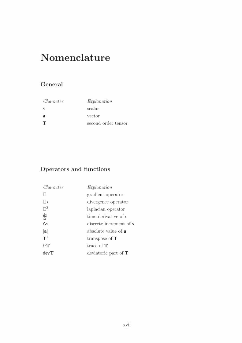
Operators and functions
Character Explanation
∇ gradient operator
∇ • divergence operator
∇2 laplacian operator∂s∂t time derivative of s
∆s discrete increment of s
|a| absolute value of a
TT transpose of T
trT trace of T
devT deviatoric part of T
xvii

xviii Nomenclature
Latin symbols
Character Unit Explanation
A analytical solution
C m/sec characteristic velocity of fluid or solid
Co Courant number
d m vector from P to N cell centre
D m displacement
E truncation error
EP W external power
f Hz frequency
F fluid
gb fixed gradient at the boundary
h m height of the beam
I unit tensor
K Pa bulk modulus
KP W kinetic power
l m length of the beam
m kg mass
n unit vector normal to a control volume face
N neighbour cell centre
p Pa pressure
P present cell centre
S solid
S m2 closed surface
S f m2 face area vector
SP W strain power
t sec time
TP W total power
U m/sec velocity vector
V m3 volume
x m position in x direction
y m position in y direction

Nomenclature xix
Greek symbols
Character Unit Explanation
A any spatial operator
δ m end displacement
ε strain tensor
ε rate of deformation tensor
η Pa
sec
dynamic viscocity
λ Pa Lame’s coefficient
µ Pa Lame’s coefficient
ν Poison’s ratio
ρ kg/m3 density
σ Pa Cauchy stress tensor
τ Pa applied end shear
φ any property (scalar, vector or tensor)
ϒ Pa Young’s modulus
ω Hz frequency of undamped oscillation
ωN weighting factor form P to N cell centre
Superscripts
Character Explanation
o old values
oo old old values
n new values
∗ spatial discretisation

xx Nomenclature
Subscripts
Character Explanation
0 reference situation
f face value
N value at neighbour cell
P value at present cell
Abbreviations
Characters Explanation
A analytical
BD backward differencing
CD central differencing
CFD computational fluid dynamics
CSM computational solid mechanics
CV control volume
EP external power
EI Euler implicit
FE finite element
FV finite volume
FSI fluid structure interaction
KP kinetic power
LCR inductance-capacitance-resistance circuit
N numerical
NM not mentioned
PDE partial differential equation
SP strain power
UD upwind differencing
Chapter 1
Introduction and literature survey
1.1 General Introduction
The term fluid-structure interaction (FSI) is a general term used to describe certain
physical phenomena. Let us first define the meaning of the term, since it is sometimes
misused. The important aspect is that there must be a genuine interaction between
a fluid and a solid component. This implies that, at the interface, a property of the
fluid influences a property of the solid and, crucially, vica versa.
This project is concerned with FSI, using the term in its most common sense, that
is interaction of forces and the corresponding movement of the interface (momentum
interaction) rather than thermal interaction. The movement of the solid because of
momentum exchange with the fluid can occur in one of two ways (Figure 1.1): by
a local deformation of the solid body, or by rigid body motion. The term FSI is
commonly used in flow of liquids in pipes to describe the effect of pressure on rigid
body motion on complete pipe structures. Extensive reviews by Tijsseling (1996) and
Tijsseling and Wiggert (2001) describe the work performed in this areas. However,
this project investigates the interaction between the local deformation of flexible
tubes and liquid pressure, in particular its effect on the propagation of pressure
waves.
Waveforms are highly dependent on the geometry of the tube. Fluid structure
interaction becomes particularly important when the liquid is almost incompressible
and deformation on the solid can not be neglected (Korteweg, 1878). Prediction
of pressure waves is particularly important in liquid filled vessels in areas such as
arterial flow, impact of filled vessels and pipelines.
The study of the wave propagation phenomenon in fluid filled flexible tubes is
often motivated by the need to understand arterial blood flow. The arterial flow is
almost unique in that it is driven by pressure waves that initiate from the contraction
of the cardiac muscle. Pulse propagation phenomena in the arteries are governed by
the interaction of the blood with the elastic arterial wall.
Many investigators have tried to analyse the wave propagation phenomena and
1

2 Chapter 1. Introduction and literature survey
Local deformationRigid body motion
Momentum interaction Thermal interaction
FSI
Figure 1.1: FSI categories.
in particular in the cardiovascular system, the resulting blood flow and and pressure
wave forms. The methods used vary from the simple windkessel model to highly
complicated multidimensional mathematical and computational models. This is not
trivial due to the fact that the hemodynamics of blood circulation is affected by many
factors such as: vessel geometry, pulsatility, flow rates, bifurcations in branches, non-
Newtonian behaviour of the blood as well as compliance of the vessel walls. For the
validation of these models there is a need for in-vivo measurements as well as in vitro
laboratory experiments in mechanically and constitutively well-defined systems.
In Section 1.2 the morphology of the arteries is described. The literature survey
is separated in two parts: the different methods used for handling the fluid-structure
coupling is described in Section 1.3 while the experimental and analytical work in
wave propagation in straight and tapered vessels are discussed in Section 1.4. Finally,
the objectives of this study is outlined in Section 1.5 .
1.2 Morphology of arteries
The blood vessels form a closed network that carries the blood away from the heart
and back. This vessel network consists of arteries, arterioles, capillaries, venules
and vains. The arteries and arterioles transfer the blood away from the heart in
order to deliver oxygen to the tissues and organs. The arteries are large vessels
that are very strong and elastic and they deform as the blood flows away from the
heart under hight pressure. They subdivide progressively to thinner and thinner
tubes and eventually end up to the finest branched arterioles. Therefore according
to their diameter can be grouped to: elastic arteries (aorta, brachiocephalic trunk
and carotid arteries), muscular arteries (all others with diameter > 0.1mm ) and
arterioles 10−100µmRoades and Tanner (1995); Levick (2000).

1.2. Morphology of arteries 3
Endothelium
Connective tissue
Tunica Intima
Tunica media
Tunica adventitia
THREE LAYERS
C.G.Giannopapa
Figure 1.2: Cross sections of the arterial wall (not to scale).
1.2.1 Wall layers
The wall of the artery consists of three distinct layers or tunics, shown in Figure
1.2, which, from inside to outside are called: tunica interna or intima, tunica media
and tunica externa or adventitia.
Tunica intima
The tunica intima or internal consists of a layer of a simple squamous epithelium
called endothelium, that rests on a connective tissue membrane that is rich in elastic
and collagenous fibres.
Tunica media
In the muscular arteries the tunica media makes up the bulk of the arterial wall. It
includes small muscle fibres that encircle the tube and a thick layer of elastic connec-
tive tissue. The connective tissue gives to the artery a tough elasticity to withstand
the blood pressure force and at the same time stretch in order to accommodate the
sudden increase of blood volume that accompanies the opening of the heart valve
due to the ventricular contraction of the cardiac muscle.

4 Chapter 1. Introduction and literature survey
Tunica adventitia
Tunica adventitia or externa is a thin layer and mainly consists of connective tis-
sue with irregular elastic collagenous fibres. This layer attaches the artery to the
surrounding tissues. It also contains minute vessels (vasa vasorum) that give rise to
capillaries and provide blood to the most external cells of the artery wall.
1.2.2 Wall dimensions
The measurement of wall thickness of the blood vessels is not a trivial task. This is
due to the fact that there is not a clear line separating the adventitia from the sur-
rounding tissues. This means that the dissection process may influence the results.
Another factor that may influence the measurements is that the vessels shrink when
removed from the body, so in order to have reliable data, they must be stretched to
their natural length before measurement.
The first measurements of wall thickness have been done under the microscope,
which has the obvious problem of maintaining the vessel in normal length and pres-
sure. Another problem of this method is the fact that the chemicals used for fixation
alter significantly the dimensions of the vessel. Another method used in the past
was based on Archimedes’ principle, which gives more accurate results. Nowadays,
there is an option of non-invasive measurement of the wall thickness using ultra-
sound. This method is though limited to measurement of thickness of intima-media
because the outer boundary of the adventitia can not be distinguished from the
surrounding tissue, as mentioned before (Hoeks et al., 1997).
One of the most referenced sources on vessel dimensions is the paper of Westerhof
et al. (1969). The morphological data presented in his work has been used as a
guidance for the design of the tubes used in this work in Chapter 5 (Table A.1).
Information about the research conducted to define the mechanical behaviour of the
blood vessels can be found in the data book of Abe et al. (1996), where a summarised
collection of papers published in the area until 1996 is presented.
1.3 Computational Methods for fluid structure in-
teraction
Typically in FSI, the fluid and solid components are modeled using different tech-
niques to different levels of complexity, ranging from simple analytical solutions to
3-dimensional numerical schemes with advanced physical models. In addition to
the range of techniques available for modelling the individual fluid and solid com-
ponents, there is also the question of exchanging information, typically in the form
of boundary conditions, at the interface. The options here are limited and can be

1.3. Computational Methods for fluid structure interaction 5
classified on the basis of the level of coupling between fluid and solid, as shown in
Figure 1.3.
• The most basic approach is non-iterative over all time (method 1). In litera-
ture it can also be found under the name uncoupled approach. The fluid and
solid equations are solved separately for the whole time domain. The fluid is
solved first to obtain velocity and pressure and the pressure at the interface
is specified as a time-varying boundary condition for the solution of the solid
equations.
• The second method is iterative over all time (method 2). It is similar to the
non-iterative approach except that the solution for the solid, i.e. displacements
or velocities, is used as a time-varying boundary condition on the fluid. The
process is repeated by solving for the fluid, passing the pressure boundary
condition to the solid, solving for the solid etc. The process can be repeated
until it converges to a point where the solutions are the same, to within a
prescribed tolerance, from one simulation to the next (i.e. from fluid to solid
and vice versa).
• The third method can be named non-iterative over each time step (method
3a). In this case, boundary conditions are passed between fluid and solid at
the end of individual time steps, but no iterations from fluid to solid solutions
take place within the time step. The time steps need not be the same for
both fluid and solid in which case, the exchange of boundary data can not
occur after each time step. This case may be referred to as non-iterative over
unequal time steps (method 3b).
• The fourth method is iterative over each time step (method 4). In this ap-
proach, the fluid equations are solved for a single time step and the pressure
solution becomes the boundary condition for the solid equations. The solid
equations are solved for the same time step and the solution obtained is re-
turned as a boundary condition for the fluid which is again solved for the
same time step. The process is repeated for that particular time step until the
system of both fluid and solid equations has converged to within a prescribed
tolerance. Only then the procedure advances into the next time step.
In the case of non-iterative over all time (method 1), non-iterative over time step
(method 3a), non-iterative over unequal time steps (method 3b), the fluid solution
preceeds the solid one; so, data transfer is one-way only, i.e. from fluid to solid.
When FSI is taken into account, fully coupled methods should be adopted. Both
fluid and solid equations should be solved simultaneously and two-way data transfer
should be performed, like in methods: iterative over all time (method 2) and iterative

6 Chapter 1. Introduction and literature survey
31 5 . . .
42 6 . . .
31 5 . . .
42 6 . . .
∆t ∆t ∆t∆t
Time TimeEndStart
METHOD 4over time stepIterative
Iterativeover all time
METHOD 2
Up
p p p p
1
2F
S
F
S
4 678
1 3 5
S
F
S
F
1 2 3 4
S
F
S
F
∆t ′
21 3 4 6 7 8 9 11 12 13 14
5 10 15
16 17 18 19
20
2
∆t ′ ∆t ′ ∆t ′
METHOD 5
Implicitsingle solution
p
p
p p
U
U U U U
U U U U
pU U U
METHOD 3btime stepsover uniqual
METHOD 3aover time step
Non-iterative
p p pp
over all time
METHOD 1
Non-iterative
Non-iterative
NOTE: The numbers in italics are counters of the computational time step. Thestraight dashed arrow represents the transfer of information of the denoted variablefrom one medium to the other. The curved dashed arrow represents the iterativeprocedure.
Figure 1.3: Solution procedure of several FSI methods.

1.3. Computational Methods for fluid structure interaction 7
F
SS S
F F
monolithicmethod
single solutionmethod
partitionedmethod
Figure 1.4: FSI methods conventional terminology.
over time step (method 4). In order to get a realistic simulation, the exchange of
information should be done at least once in each time step.
In the discretisation process there are two issues involved, the treatment in time
and space. Detailed discussion about the choice of discretisation methods used
to solve the partial differential equations describing the problem is presented in
Section 3.1. Looking at the time treatment of the fluid and solid, according to the
conventional terminology found in the literature, current numerical methods can
be grouped in two major categories: Partitioned methods and monolithic methods
(Figure 1.4).
The partitioned methods are based on partitioning the fluid and the solid solu-
tion, the fluid and structural equations are solved alternately and the enforcement of
kinematic and dynamic interface conditions is asynchronous. It is typical for these
methods that two separate software packages are used for modelling the solid and
the fluid. The integration of two software codes is possible in principle, but the com-
plexity and size of the software make this approach quite unattractive. Furthermore,
the computational overhead to run such codes is quite exorbitant as information has
to pass from one code to the other in each time step, adding to the total overhead
(Belytschko et al., 1986). Data transfer usually requires an extra program that acts
as an interface between the other two codes, thus sacrifices the modularity of the
method. In the fluid structure interaction community, some researchers have focused
in utilising a modular approach of the interface program for the exchange of informa-
tion between two codes (Farhat et al., 1998, 2001; Raveh, 2000). Such an approach
is often called modular approach. An overview of the benefits and disadvantages
of using these methods can be found in Felippa et al. (2001). Partitioning leads
inherently to loss of conservation of properties of the continua (fluid and structure).
The energy increase in the system leads to instability which is the major drawback
of this method.
The monolithic methods use two separate sets of equations for fluid and solid
and couple the fluid dynamics and structural dymamics implicitly and solve them

8 Chapter 1. Introduction and literature survey
syncronously at the their common interface (Tallec and Mouro, 2001; Hubner et al.,
2004; Bloom, 1998; Alonso and Jameson, 1994; Rifai et al., 1998). The discretised
equations are solved by subiteration until convergence within one time step. These
methods can be unconditionaly stable and energy conservative (van Brummelen
et al., 2003) when the modified Osher scheme is used for the fluid elements (van
Brummelen and Koren, 2003). These methods are quite complex and computation-
aly expensive due to the subiteration.
The single solution method proposed in this thesis is quite different from the
partitioned and the monolithic methods. Figure 1.4 assists the reader with the con-
septual and computational understanding of this novel approach and its differences
from the conventional methods. The single solution solution methods treats both
fluid and solid as a continium, thus the whole computational domain is a single
entity in a single grid. Its behaviour is described by a single set of equations and
is solved fully implicitly. There is no explicit exchange of information between the
fluid and solid interface as it is inherently implicit. In this way, the computational
expence of the subiterations of the monolithic approach is expected to be avoided.
The difficulty that lies with this method is the conceptual understanding of using
a single set of equations to describe both fluid and solid, the choice of this single
set of equations and the choice of appropriate boundary conditions. The creation
this single set of equations can be done in one of two ways: use the solid as the
prime model and reformulate the equations of the fluid to match the ones for the
solid or the other way around. In this thesis the later approach is chosen as it was
considered to be more natural for flexible vessels. In a single solution method, the
distinction between the state of the continium (fluid or solid) is associated with
different coefficients in a single set of equations (Section 2.4).
Early studies on wave propagation of incompressible fluids in elastic tubes, like
rubber hose and blood vessels can be found in Young (1808) and for compressible
fluids in Korteweg (1878).
Even though the basic equations and the first theories date back to the 19th
century, only in 1970s, with the introduction of computers, could the basic FSI
equations be solved. Nowadays with the continuous advancement of computer power,
special-purpose commercial, as well as ’in-house’, codes exist in the area of FSI.
Reuderink et al. (1989) were amongst the first researchers to compute pulsatile
flow in elastic arteries based on one dimensional wave propagation. They applied
both linear and non-linear theory in blood vessels and compared them with experi-
mental data. It was found that the linear model seemed to be more appropriate, since
damping of the wave can be accurately described in the linear model. Nonetheless
the non-linear terms in mass and momentum conservation equation may be signifi-
cant.

1.3. Computational Methods for fluid structure interaction 9
Perktold and Rappitsch (1995) used an iterative approach for the same flow field
examined by Reuderink et al. (1989). The boundary conditions of the flow problem,
the inlet and the outlet pressure, were obtained from experimental data. They
compared the results from models using rigid and distensible wall and they found
that the distensible wall model gave more realistic results.
Steinman and Ethier (1994) adopted a similar approach to Perktold and Rap-
pitsch (1995). They used an analytical approach to study the effect of wall dis-
tensibility of a flow on end-to-side anastomosis. The outlet pressure was obtained
by wave theory. Comparing their results with rigid-wall simulations, they found
moderate changes in the wall shear stress. According to them, models that neglect
the wall distensibility are less useful for predicting the behaviour of local pressure
gradient fields as well as velocity profiles.
Henry and Collins (1993a,b) were concerned with the prediction of wall move-
ment in elastic tubes using an iterative approach as a coupling method. The inlet
and the outlet pressures were fixed to a certain value. The model was validated
against analytical solutions.
Taylor et al. (1998) used a numerical method to model only the fluid of a pul-
sating flow in straight arteries. For boundary conditions of the fluid-solid interface,
they used zero wall motion. The numerical method was validated against Womersley
(1957) analytical solution. They were concerned that the methods available for FSI
produced enormous amount of data and took a considerable amount of computa-
tional time. In their opinion, these should be reduced and better engineered codes
should be adopted.
Bathe and Kamm (1999) used the ”iterative over time step” coupling approach
in modelling pulsatile flow in stenotic arteries. Boundary conditions at the inlet and
outlet were obtained from experimental data. Their model was compared with other
mathematical models and was validated against experimental data. They compared
arteries with different degrees of stenoses. They found that the inviscid predictions
were naturally lower than the computed pressure drops due the fact that the viscous
losses are neglected. They found that the bulk of the pressure drop into the stenosis
is due to the convective acceleration of the flow.
Konig et al. (1999) modeled only the fluid using a moving boundary. Inlet and
outlet pressures were fixed to reference values. Their model was validated against
experimental data. They compared high and low viscosity models and obtained
better results with the high viscosity model.
Tang et al. (1999a,b) studied stenotic arteries by using both thick and thin wall
models. They noticed that the stenotic severity and asymmetry in thick wall models
changed not only the wall geometry, but also the stiffness of the tube wall and
this affected the wall deformation. The maximum shear stress from the thick wall
asymmetric stenotic tube was considerably lower than that from thin wall model

10 Chapter 1. Introduction and literature survey
due to increased stiffness of asymmetric stenosis. They came to the conclusion
that arteries have a complex structure and should not be treated as a homogenous
material.
Zhao et al. (1998) and Xu et al. (1999) used both thin and thick wall models
and showed that the thick wall model provides more realistic results. The compu-
tational model is compared with data obtained from Magnetic Resonance Imaging
(MRI) scanning of real patients. They state that it is difficult to make a direct
comparison because of the large variations in anatomy of the patients. The model
takes into account neither the compliant behaviour of the vessel wall nor the non-
Newtonian behaviour of the blood, as the authors consider these to be of a secondary
importance.
Greenshields et al. (1999) presented a finite volume (FV) method for solving
three dimensional equations for both fluids and solids. They used the iterative
coupling using unequal time steps (method 3b). The exchange of information at the
interface was done in an explicit manner which is the main limitation of their model.
The method was capable of predicting in detail the start of a propagation pressure
wave accounting for two dimensional and pipe resonance effects. It was potentially
unstable for extremely flexible structures such as arterial walls.
The assumptions used in the literature to model the fluid and the solid compo-
nents have been identified and are summurised in a tabular form in Table 1.1.
1.4 Wave propagation in flexible vessels
The main focus of this section of the literature review is wave propagation in flexible
vessels from a theoretical as well as experimental point of view. The literature
review is separated in four parts: theoretical wave propagation in straight tubes;
experimental wave propagation in straight tubes; theoretical wave propagation in
tapered tubes; and experimental wave propagation in tapered tubes.
1.4.1 Theoretical models on straight tubes
Young (1808) was the first investigator interested in understanding the transient
motion of fluids in pipes, elastic tubes, conical vessels and blood circulation. He
proposed a formula for the velocity of pressure waves in an elastic tube with thin,
homogenous and isotropic wall, filled with an incompressible fluid.
Witzig (1914) has also investigated the wave propagation by modelling thin-
walled flexible tube by solving two dimensional linearised Navier-Stokes equations.
He was the first one to show the effects of viscosity of the fluid and present fluid
velocity profiles.
The work of Womersley (1957) is the most referenced one in the literature and has

1.4. Wave propagation in flexible vessels 11
REFERENCE
CHARACTERISTIC Reu
der
ink
etal
.(1
989)
Per
kto
ldan
dR
appit
sch
(199
5)
Hen
ryan
dC
ollins
(199
3a,b
)
Tan
get
al.(1
999a
,b)
Ste
inm
anan
dE
thie
r(1
994)
Kon
iget
al.(1
999)
Tay
lor
etal
.(1
998)
Bat
he
and
Kam
m(1
999)
Xu
etal
.(1
999)
SolidsNon linear
√ √ × × × NM NM√ ×
Viscoelastic√ × × × × NM NM
√ ×Compressible
√ √ × × √NM NM × ×
Large strain × × × × × NM NM√ ×
Thick wall × × √ √ × NM NM × √
3 Dimensional × √ √ √ × NM NM√ √
Method A FE FV FE A NM NM FE FEFluids
Non Newtonian × √ × × × × × × ×Compressible × × × × √ × × × ×
Turbulent × × × × × × × × ×Transient
√ √ √ √ √ × × × ×3 Dimensional × √ √ √ × √ √ √ √
Method A FE FV FE A N N FE FV
NOTE: The symbol√
denotes that the characteristic in the left column has beentaken into consideration, whereas the × means that is has not.
Table 1.1: Modelling assumptions for the fluid and solidcomponent as found in the literature.

12 Chapter 1. Introduction and literature survey
been extensively compared against other theoretical models and further extended.
Womersley (1957) solved the two-dimensional linearised Navier-Stokes equations for
thin-walled isotropic infinitely long elastic tubes filled with viscous Newtonian fluid.
He studied both unrestrained tubes and tubes constrained in the axial direction. An
extensive overview of the work performed in this area can be found in McDonald
(1968); Cox (1969); Pedley (1980); Tijsseling (1996); Wood (1999) .
Atabek and Chang (1961) studied analytically the unsteady flow near the entry
of a circular tube and showed that the entry length varied with the time through
the cycle, as do the boundary layers which determinate it. Their findings were
assessed computationally and extended by Ku et al. (1990). Klip et al. (1968)
studied non-axisymmetric wave propagation in compressible fluids using a thick
wall viscoelastic tube. Atabek and Lew (1966) extended the Womersley theory to
initially stressed thin walled tubes in the axial and circumferential direction. They
mention the existence of two waves: radial and longitudinal that can be found with
the Womersley theory even though he did not mention this himself. Using the
continuity and momentum equation the frequency equation can be obtained. The
two roots of this equation will give the velocity of the propagation of the two waves.
Mirsky (1968) used the Womersley models with longitudinal tethering and ex-
tended it to include tubes with orthotropic walls. Cox (1969) reviewed the work
performed in this area until then by dividing it in three categories: thin-wall with
no constraint; thin-wall with longitudinal constraint and thick walled tubes. He pre-
sented a table comparing the different theoretical models developed by that time.
Atabek (1968) continued the work using the membrane theory of shells on or-
thotropic tubes. He found that the propagation properties of the slower waves are
very slightly affected by the degree of anisotropy of the wall. For the faster waves
the velocity of propagation decreases as the ratio of the longitudinal modulus of
elasticity to circumferential modulus decreases. When tethering is used, the faster
waves are completely attenuated, while the slower ones are hardly affected. His
findings were in good agreement with the Womersley theory and the work of Mirsky
(1968). He pointed out that in order for the theory to be complete and realistic
for use in an arterial system there is a need to include taper, branching and the
viscoelastic properties of the wall. The theories should be validated against well
defined experimental data that were lacking at the time.
Ling and Atabek (1972) introduced the nonlinear terms of the Navier-Stokes
equations as well as the nonlinear behaviour and large deformations of the arterial
wall. They also performed experiments. From the comparison of the experimental
data with the linear and non-linear model, they concluded that their non-linear
theory predicts the velocity profiles much better than the linear one. The wave of
the wall shear predicted by the linear theory is very close to the one predicted by
the non-linear theory. Their model was assessed computationally by Dutta et al.

1.4. Wave propagation in flexible vessels 13
(1992).
Blood circulation has also been studied by comparing it with other physical
models employing hydro-dynamic and electrical analogies. A review of such models
can be found in Westerhof et al. (1969). Westerhof et al. (1969) modelled the
entire arterial tree, discarding the viscous behaviour of the vessel, using an electrical
analogue and compared it with clinical measurements. He concluded that reflections
occur at all branch points and play a major role in determining the behaviour of
the system. He showed how the nature of the input impedance and wave traveling
pattern can be explained in terms of these reflections. He also published full data
of human tree physiological parameters.
1.4.2 Experimental models on straight tubes
There is a vast literature involving in-vivo measurements in animals and humans,
using open-chest measurements or using other techniques such as MRI scanning,
but since they are beyond the scope of this project, they are not be mentioned
here. The interest of the investigation is focused on experiments with flexible tubes.
Rubber-like materials have been quite popular in modelling arteries, as the modulus
is similar to that of human arteries.
von Kries (1883) was interested in measuring the pressure pulse in human bodies.
He performed experiments on a rubber hose in order to validate his theory. He used
a 4 to 5 m long, thin-walled rubber hose of 5 mm diameter supplied with water
through a constant-head reservoir.
Klip (1962), realising that propagation velocity and damping of pressure waves
in arterial systems can be used for diagnostic purposes, performed a series of ex-
periments on tethered tubes of great length. He used a homogeneous, isotropic,
viscoelastic tube of more than 60 m long. A piston was used to initiate a pres-
sure wave. For about 4 m after the piston the tube was kept straight and the rest
was wound up in a spiral. No reflections were present. The tube was filled with
different water-glycerine solutions. Pressure was measured with a manometer and
phase differences with an electric phasemeter. He considered both thick wall and
thin wall tubes. He compared his data with other methods of calculation for the
phase velocity and he found that they were in good agreement with Womersley’s
results as well as with Moes-Korterweg predictions. Discrepancies were present for
damping, however.
Ling and Atabek (1972) were interested in simulating blood flow in dogs with
an experimental rig. They used a composite straight structure of silicon rubber and
corrugated nylon fibres. The tube diameter was appropriate for a medium sized
dog and the thickness of the tube was 1mmwith ±0.1mmvariations. They used a
glycerin-water mixture as a fluid. The pressure and pressure gradient were measured

14 Chapter 1. Introduction and literature survey
using two pressure transducers at a 50mmdistance from each other. Velocity pro-
files were measured using a hot-film velocity probe. Wall shear stress was measured
as well. The pressure-radius relation was obtained by photographing simultane-
ously the inflation of the vessel and the pressure signal, using an 8mm cine camera
equipped with high power photography.
Nerem et al. (1971) investigated the transition to turbulence in the aorta and
related the results to equivalent steady flow ones in which the similarity parameters
were the wave number and the Reynolds number.
Liepsch and Moravec (1984) prepared a rubber replica of the femoral artery and
performed experiments of pulsatile flow. Deters et al. (1986) made a silicon rubber
cast from luminal mould of an aortic bifurcation. They measured phase fluid velocity
by LDV at a single point close to the wall. The motion of the wall was obtained by
integrating the velocity. The shear rate at the wall was estimated by dividing the
fluid velocity by the distance from the velocity measurement point to the wall.
Up to that time the Womersley theory had been tested only for tethered tubes.
Gerrard (1985) was interested to determine the behaviour of infinitely long tubes,
where the longitudinal motion was present. In his set up, he used isotropic latex
rubber tubes, with small viscoelasticity. He glued together two tubes of 15m length,
inner diameter of 6.2mm and thickness of 1.8mm. The tube was filled with water.
A wave was initiated by a piston at one end and the other end was closed. The
free motion of the tube was obtained by suspending it from the ceiling with cotton
sewing threads 100mm apart. This tube behaved like a semi-infinite one over almost
all its length. No reflections were present. From the comparison of the experimental
data with Womersley theory for an infinite tube with no constraint it was concluded
that the experimental data were in good agreement beyond the entrance length.
There were some discrepancies though, near the end of the tube. That was an
indication that there may be an end effect at the closed end far from the piston,
which considerably reduces the amplitude calculated from the infinite-tube theory.
He also performed experiments on tethered tubes of 30m long and found that his
measurements were in good agreement with those of Klip (1962).
van Steenhoven and van Dongen (1986) were interested, apart from wave prop-
agation phenomena, in aortic valve closure. They performed experiments on water
filled latex tube 0.6m long with 18mm inner-diameter and thickness 0.2mm. Trans-
mural pressure was applied at one end of the tube. Pressure was measured using
two catheter-tip manometers. Wall deflection was measured using a photonic sen-
sor and the flow volume was measured electromagnetically. The fluid was suddenly
stopped locally starting from steady flow. The measurements describing the wall
behaviour were in good agreement with those of Gerrard (1985). From their mea-
surements they obtained the viscoelastic properties of the tube. The compared their
experimental data with the one dimensional non-linear theory for the wall shear

1.4. Wave propagation in flexible vessels 15
stress, that was solved numerically using the method of characteristics. They wall
was treated as viscoelastic and wave reflections were also taken into account. From
the experiments they concluded that the wall viscoelasticity is a dominant factor in
the gradual flattening of the waveform. They also mention that the local change
in compliance generates expected wave reflections and has strong influence on the
rise-time of the wave front. The most important consequence is that the pressure
jump of the wavefront decays while propagating upstream.
Horsten et al. (1989) used for their experiment the same experimental setup
and the same tube as van Steenhoven and van Dongen (1986) but 0.9m long to
simulate wave propagation. They compared their experimental data with one di-
mensional linear theory with focus on the viscous phenomena of the fluid and tube
wall and found them in good agreement for small pulsed shape waves. They com-
pared and assessed different linear models on their performance in describing the
wall behaviour and it was found that there were no major deviations amongst them.
They concluded that the one dimensional Womersley linear theory, where the fluid
is treated as incompressible, describes fairly well the propagation phenomena. The
wave velocity, though, was underestimated and the damping was overestimated. The
discrepancies between experimental and analytical data are partially explained by
the non-linearities. The rigid support of the tube could be another explanation of
the discrepancies.
Reuderink et al. (1989) also focused on assessing the one dimensional linear and
non-linear theory describing the pulse wave propagation in a uniform viscoelastic
tube. A 1m long latex rubber tube filled with a salt solution was used. A pneu-
matically driven piston was used for the pulse initiation. A catheter tip manometer
was used for measuring the pressure at different positions along the tube. They at-
tempted to measure pulsatile diameter changes using an ultrasonic transit-time tech-
nique but they stated that the influence on the wall motion was present, even though
minimised. The experimental data showed that the pressure vs cross-sectional area
relation was nonlinear for the pressure changes. By comparison of the experimental
data with the linear and non-linear models they came to the conclusion that in spite
of the nonlinearity of the system, the linear viscoelastic Womersley model described
the pulse wave propagation satisfactorily. They explained that the discrepancies be-
tween the experimental findings and the prediction of the non-linear model are due
to the fact that frictional losses due to the wall viscoelasticity are neglected and due
to fluid viscosity are underestimated. Therefore, non-linear models predict small
damping and formation of shock waves, which were not observed experimentally.
16 Chapter 1. Introduction and literature survey
1.4.3 Theoretical models on tapered tubes
The need to capture the nature of the arterial tree and define its physical properties
in order to use them as the correct parameters in modelling, have lead to investiga-
tion of the geometrical tapering of the tubes. Young (1808), was one of the first to
mention possible effects in the blood circulation. Taylor (1965) was concerned with
wave propagation in a non-uniform transition line.
Wemple and Mockros (1972) solved a one dimensional non-linear mathematical
model by the the method of characteristics. Their non-linear model included geo-
metric and elastic taper of the flexible tube. They compared their model with data
measured in humans. The elastic taper theoretically affects the wave transmision
and reflection in the same way as to that of geometric taper. The degree of the
elastic taper is small compared to that of the geometric taper, therefore they con-
cluded that the elimination of the elastic taper does not have significant effects on
the model. The geometric tapering on the other hand is quite important for the
presence of reflection waves. They concluded that the system behaves in a linear
way for the lower frequencies, while for the higher frequencies the non-linearities are
important. The linear theory is unable to deal with tapered tube if the pressure
pulse is high.
Belardinelli and Cavalcanti (1992) used a two dimensional non-linear model.
They point out that the natural tapering of the arteries should be taken into account
as it has been indicated from in-vivo measurements. Their model encompasses the
motion of a pulse-driven viscous fluid in a geometrically tapered flexible tube. They
make the assumption of uniform pressure in a cross section. Their results show
that the tapering does not influence the wave velocity but it influences the waves’
attenuation rate. They used infinite extremity impedances to maximally enhance
the reflections so that the overall attenuation is only due to arterial properties and in
particular the natural tapering. The natural tapering causes a continuous increase
in the pulse amplitude as it moves from one side of the tube to the other. In a 0.6m
long tube with taper angle of 0.1 the pulse amplitude at the end of the tube is more
than twice the input pulse. The reflected pulse is greatly damped and its shape is
quite different from that of the direct pulse.
Einav et al. (1988) used an LCR (inductance-capacitance-resistance circuit) elec-
trical analogue to study wave propagation in exponentially tapered tubes with main
interest in reflections at bifurcations. Their model was compared with the one of
Westerhof et al. (1969). They concluded that the input impedance is low for high
frequencies. Therefore, blocked branches in the vicinity of the heart do not signifi-
cantly contribute to the input impedance. More distal bifurcation, such as the ileac
bifurcation, can affect the input impedance at low frequencies. From their reflection
condition they conclude that in order to maintain continuity in a junction, the char-
acteristic impedance and peripheral impedance are doubled and the cross-section of

1.4. Wave propagation in flexible vessels 17
the branches is 15% larger than the main branch.
Chang et al. (1994) used the electrical analogue in which they included the
non-uniform properties of the tube, as well as the geometric and elastic tapering.
They compared their model with in-vivo measurements in dogs. They found good
agreement between their impedance parameters derived by their non-uniform model
and the ones measured in the animals. Comments about their work can be found in
Burattini et al. (1996).
Fogliardi et al. (1997) used an exponentially tapered electrical analogue to model
descending aortic circulation. In their model they used five parameters to charac-
terise the input impedance: the characteristic impedance, the compliance of the
tube, the tube length, the tapering, the time constant of the load and the peripheral
resistance. They performed open chest in-vivo measurements in dogs to obtain pres-
sure and flow measurements. From the comparison of their model with the in-vivo
data they found that the tapered tube models showed a slightly closer matching
with the experimental flow and the reproduction of the input impedance.
1.4.4 Experimental models on tapered tubes
After a thorough survey of experiments performed with tapered tubes, the author
found a vast amount of literature of in-vivo measurements in humans and animals
but only two papers studying wave propagation in geometrically tapered elastic
tubes: von Kries (1892) and Reuderink et al. (1988).
von Kries (1892) was interested in understanding blood pressure waves. He was
the first one to perform experiments on a rubber tapered tube. He had two straight
tubes of 22 mm and 5.5 mm diameter connected to each other by a 140 mm long
conical part. His interest was to use tapering to eliminate the wave reflections of a
pressure wave form when transmitted from a tapered tube to a straight one.
Reuderink et al. (1988) used a uniform latex tube 0.5m long with 12.73mm outer
diameter and thickness 0.14mm with a variation of ±0.01mm for the straight tube;
the tapered one varied from 15.88 to 9.45mm outer diameter (46 degrees taper)
with horizontal to vertical slope of 0.008 and thickness 0.13mm ±0.01mm. The
tubes were manufactured by dumping the mould in latex rubber. The working
fluids used were salt solutions of different concentration and glycerine solution. The
salt solutions were used in order to be able to measure electromagnetically the flow.
A pneumatically driven piston was used for the pulse initiation. Impulse or sine
waves were used for the excitation. The sine wave did not produce a steady flow
component. A catheter tip manometer was used for measuring the pressure at
different positions along the tube.
They compared the real part of the true propagation coefficient with the appar-
ent damping and the damping coefficient calculated from Womersley theory. They
18 Chapter 1. Introduction and literature survey
also compared the true phase velocity with the measured apparent phase velocity,
foot-to-foot velocity, and calculations of phase velocity parameters using the Wom-
ersley’s theory and the Moens-Korteweg equation. From their comparison they
conclude that the three point method used to obtain the propagation coefficient is
in agreement with all other estimate for a uniform tube. For a tapered tube the
three point method causes an error estimation of the propagation coefficient. They
state that in their experiments tapering only cannot take account for the differences
between in-vivo measurements of the propagation coefficient using the three-point
method and calculations based on the Womersley’s theory since in their results taper
caused a discrepancy only at some frequencies, and at these frequencies the damping
was largely underestimated instead of overestimated.
1.4.5 Concluding summary
The complexity of the physical phenomena and the simultaneous interaction of var-
ious effects make a complete analysis of blood flow almost impossible. Certain
assumptions are necessary but they have to be verified. Validation of the theoretical
models and assumptions can be done through comparison with in-vivo and in vitro
measurements.
In-vivo measurements have obvious limitations like: handling of the subject,
conditions of measurements, law restrictions etc. On the experimental side, one is
usually limited to measure only a small fraction of the quantities of interest and
even then they can be sampled only at a few times and special locations, with a
limited degree of accuracy. Therefore it is important that well defined experiments
are carried out.
The most dominant theoretical model with numerous extentions in wave prop-
agation in flexible vessels is that of Womersley. The theory of Womersley for infi-
nitely long tubes, with or without tethering, has been experimentally validated by
the work of Klip (1962)(longitudinal constraint) and Gerrard (1985)(no longitudinal
constraint). They both verified its validity beyond the entrance length. For tubes
with finite length the theory of Womersley and its extentions has been validated
thoroughly against other theoretical models and experimental data.
Nevertheless, in wave propagation, there is a number of quantitative questions
that have not been answered satisfactorily yet. There is a lack of quantitative
agreement between measurements and theoretical models. For the prediction of
pressure wave velocity, the linear theory gives good agreement with experimental and
in-vivo measurements. On the other hand, accurate predictions of the attenuation
rate with distance along a given named vessel of the arterial pulse is doubtful. The
measured pulse consists of forward-going components and reflected components,
due to the closed end in finite tubes. Incorrect modelling of reflections leads to

1.4. Wave propagation in flexible vessels 19
REFERENCE
CHARACTERISTIC Reu
der
ink
etal
.(1
989)
Ste
inm
anan
dE
thie
r(1
994)
Ger
rard
(198
5)
Klip
(196
2)
Wes
terh
ofet
al.(1
969)
Ata
bek
(196
8)A
tabek
Lin
gan
dA
tabek
(197
2)
SolidsNon linear
√ × × × × × √
Viscoelastic√ × × × × × √
Compresible√ √ × × √ √ ×
Large strain × × × × × × √
Thik wall × × × √ × × ×Dimentions 1 2 - - - 1 1
Method A A E E A&E A A&EFluids
Non Newtonian × √ × × × × ×Compresible × × × × × × ×Turbulent × × × × × × ×Transient
√ √ √ √ √ √ √
3 Dimentional 1 2 - - - 1 1Method A A E E A&E A A&E
NOTE: The symbol√
denotes that the characteristic in the left column has beentaken into consideration, × means that is has not and − means that it is not men-tioned.
Table 1.2: Assumptions for the fluid-solid components for straighttubes as found in the literature.

20 Chapter 1. Introduction and literature survey
REFERENCE
CHARACTERISTIC Hor
sten
etal
.(1
989)
van
Ste
enhov
enan
dva
nD
onge
n(1
986)
Bel
ardin
elli
and
Cav
alca
nti
(199
2)
Wem
ple
and
Mock
ros
(197
2)
Reu
der
ink
etal
.(1
988)
SolidsNon linear × √ √ √ √
Viscoelastic × √ × √ ×Compresible
√ √ × √ √
Large strain × × × × ×Thik wall × × × √ ×
Dimentions 1 1 2 1 -Method A A A A E
FluidsNon Newtonian × × √ × ×
Compresible × × × × ×Turbulent × √ × × ×Transient
√ √ √ √ √
3 Dimentional 1 2 2 1 -Method A A A A E
NOTE: The symbol√
denotes that the characteristic in the left column has beentaken into consideration, × means that it has not and − means that it is not men-tioned.
Table 1.3: Fluid-solid assumptions for tapered tubes as found inthe literature.

1.5. Objectives of this study 21
incorrect calculation of the reflection coefficient. The incorrect characterisation of
the tethering of the tube is also one of the reasons that these discrepancies between
theoretical, experimental measurements and in-vivo measurements may occur.
Another reason for these discrepancies is the presence of physical non-linearities,
which are modelled incorrectly. The arterial system is geometrically and thermody-
namically non-uniform (Pedley, 1980; McDonald, 1968). It has continuous variations
in cross-sectional area and distensibility (compliance), as well as repeated branching.
Non-linearities are introduced in the system due to the dependence of pressure
on the above factors. There is no question that geometric and elastic tapering are
significant aspects in the arterial system. Due to the tapering, the local compliance
of blood vessels decreases with distance from the heart, whereas the characteris-
tic impedance increases. Wemple and Mockros (1972) state that in spite of the
numerous non-linearities in the system, it behaves in somewhat linear fashion for
lower frequency components (at 80 beats per second). At high shear rates, however,
non-linearities are important.
A quantitative agreement of in-vivo measurements, experiments and analytical
models has to be achieved in order to check the importance of these physical non-
linearities of the arterial system and before one decides whether to neglect them
or not. This can only be achieved by producing reliable data through well de-
fined experiments. There is a number of theoretical models taking into account the
non-linearities of the arteries. The validation of these models is limited to in-vivo
measurements, the accuracy and the conditions which are quite difficult to asses. It
is explicitly stated in the literature that there is insufficient data for non-linear tubes.
Only the work of (von Kries, 1892; Reuderink et al., 1988) was found by the au-
thor to be concerned with experiments taking into account geometric non-linearities
simultaneously with flexibility.
The elastic taper affects wave transition and reflection in a manner that is theo-
retically similar to that of geometric taper. The degree of elastic taper in the system
is small relatively compared to the geometric taper. Thus, it is important to inves-
tigate geometric taper in wave propagation. Therefore, one of the objectives of this
work is to obtain reliable experimental data on geometrically tapered tubes that
would help the further development and validation of theoretical and computational
models.
1.5 Objectives of this study
The objectives of this study are both computational and experimental and aim at
filling existing gaps in the literature.
The use of two separate solution methods for solving FSI problems leads to case-
specific codes and to problems regarding the efficiency of the coupling of the two

22 Chapter 1. Introduction and literature survey
methods, as already explained. There is a need for general purpose codes that will be
better engineered, more flexible, and be able to solve the equations for both the fluid
and the solid components simultaneously. In order to obtain a robust FSI modelling
method, suitable for general applications, the use of a single solution environment
for Fluid and Solid needs to be adopted (method 5) (see Figures 1.3 and 1.4).
In the context presented above, the first objective of the thesis is to contribute
towards the development of such a unified approach by reformulating the equations
for solids as to contain the same unknown variables as the ones for fluids, namely
velocity and pressure. In this way the solution at the interface can be obtained in
an implicit manner, thus the fluid-structure domain can be considered as a single
entity described by a single set of equations. It is expected that the new formulation
for solids will be suitable for modelling a variety of FSI applications such as blood
flow in deforming arteries, container impact, pipeline surge etc.
The second objective is to develop and test a stable and robust numerical method
for the discretisation and solution of the reformulated equations for solids. The
method should be compatible with the one used for the solution of the fluids equa-
tions.
The third objective is to test the accuracy of the developed method for dynamic
structural problems.
Finally, the fourth objective is to collect a detailed experimental data set that can
be used for the next step of the validation of the unified approach in fluid-structure
interaction problems.
The experimental work is also motivated by the need to understand further
arterial blood flow. Although the general principles governing the arterial hemody-
namics are well known (McDonald, 1968; Pedley, 1980), there are some questions
that have not yet been satisfactory answered. Amongst these is the assessment of
non-linearities arising from wall thickness variation and geometric tapering that are
naturally present in the arterial tree morphology. The main reason for this are the
apparent limitations of in-vivo measurements in combination with the lack of well
defined laboratory experiments in the literature, as explained in the previous Sec-
tion 1.4. Thus, there is a need for such experiments so as to help the validation and
further development of theoretical and numerical models.
Thus, the experimental part of this work aims to cover this gap and to assess the
linear theory which is widely used in wave propagation phenomena. The main inter-
est is to investigate the effect of geometric tapering and wall thickness variation of
flexible vessels. The experimental data can be used for the assessment of computa-
tional methods to check whether they can cope with the anatomical non-linearities.

1.6. Outline of the thesis 23
1.6 Outline of the thesis
In Chapter 2 the mathematical framework for a single solution method for fluid
structure interaction problems is developed and presented. In Chapter 3, general in-
formation about the discretisation method used for the solution of the mathematical
model is presented. In this chapter a stability analysis of the single solution method
is also presented in order to check theoretically the amount of dissipation that the
method introduces. In Chapter 4, the validation case used for the mathematical
model is described and the results obtained from the code developed are presented
and discussed. In Chapter 5, the experimental methods of the wave propagation
experiments are described and the measurements obtained are presented. The tube
manufacturing, the experimental set up and the protocols are also explained. In
Chapter 6 a comparison between the experimental measurements for straight tubes
with the linear methods is presented. In Chapter 7, the conclusions of the completed
work according to the project objectives are outlined. Suggestions for extending the
present work are also highlighted.

24 Chapter 1. Introduction and literature survey
Chapter 2
Mathematical formulation of a
unified framework for fluids and
solids
2.1 Introduction
The equations describing the behaviour of a Hookean solid and a Newtonian fluid
(Section 2.2) are typically solved for displacement and for velocity and pressure
respectively. This is due to the fact that the stress tensor in solids is defined in
terms of displacement while, in fluids in terms of velocity and pressure. In order
to obtain a single solution method, both fluid and solid equations should be solved
for the same variables. The convective nature of displacement and the nature of
pressure in fluids leads to the decision of altering the solid formulation so as to
contain as unknown variables velocity and pressure.
In the mathematical model described here, the constitutive equations for solids
are reformulated by introducing first velocity instead of displacement and second
the hydrostatic pressure, in order to express the stress tensor (Section 2.3).
In the following subsections, the governing equations are presented as well as the
developed mathematical model. For the basic background of tensor mathematics one
can refer to Adams (2003); Aris (1962) and for continuum mechanics to Chadwick
(1976).
2.2 Governing Equations
Solids and fluids are both continua, whose behaviour can be described by the same
continuity and momentum equations. There are no simplifying assumptions in the
momentum and continuity equations for fluids and solids and both are treated as
compressible. Only the constitutive laws are different. Therefore, thes will be pre-
25

26 Chapter 2. Mathematical formulation of a unified framework for fluids and solids
sented separately. Details can be found in most continuum mechanics test books,
such as Malvern (1969) and Segel (1977). The constitutive law for solids presented
here assumes a linear elastic (or Hookean) solid and provides the stress-strain rela-
tionship. The constitutive law for the fluid assumes a linear viscous (or Newtonian)
fluid and provides a relation between stress, thermodynamic pressure p and rate of
deformation tensor (ε).
Continuity equation or mass conservation
∂ρ∂t
+∇ •(ρU) = 0 (2.1)
Momentum equation (neglecting body forces)
∂ρU∂t
+∇ • (ρUU) = ∇ •σ (2.2)
Constitutive equations for linear elastic or Hookean solid
A linearly elastic solid is considered and so there is a one to one relationship between
the state of stress and the rate of strain. If the material is elastically isotropic, i.e
the elastic constants are the same for all possible choices of Cartesian coordinates,
then the generalised Hooke’s law is obtained:
σ = 2µε+λtr(ε)I (2.3)
where µ and λ are Lame’s coefficients, which are related to Young’s modulus of
elasticity and Poison’s ratio ν, by the following equations:
µ=ϒ
2(1+ν)(2.4)
and
λ =νϒ
(1+ν)(1−ν) for plain stressνϒ
(1+ν)(1−2ν) for plain strain and 3D(2.5)
Constitutive equations for linear viscous or Newtonian fluid
For a viscous Newtonian fluid the stress tensor can be determined by the pressure
and the deformation rate tensor with the following linear relationship:
σ = 2ηε+ξtr(ε)− pI (2.6)
where the viscosity coefficients ξ and η (dynamic viscosity) are related to the
bulk viscosity k = ξ +2/3η. The deformation rate tensor is the symmetric part of

2.3. Mathematical Model 27
the velocity gradient tensor i.e. ε ≡ sym(∇U)≡ 1/2[∇U+(∇U)T
]. Thus, Equation
2.6 reads:
σ = η∇U+η(∇U)T +ξtr(∇U)− pI (2.7)
For flow analysis we usually make the Stokes condition assumption k = 0, thus
Equation 2.7 reads:
σ = η∇U +η(∇U)T− 23
ηtr(∇U)− pI (2.8)
or
σ = 2ηdev(sym(∇U))− pI (2.9)
Barotropic relationship
When interested in the wave propagation in a material, it is important to define
the equation of state for a barotropic fluid and a compressible solid, showing the
relationship between the density and the thermodynamic pressure in the fluid or the
solid. This relationship can be derived by the definition of the bulk modulus K in
the material:
K = ρ∂p∂ρ
⇔ ∂ρ∂p
=ρK
(2.10)
For small variations of density about a reference density ρ0, we can assume
that ρ ≃ ρ0, so Equation 2.10, can be linearised giving the linearised form of the
barotropic relationship:
ρ ≈ ρo
[1+
p− p0
K
](2.11)
where p0 is the reference pressure and ρ0 is the initial density for which ρ(p0) = ρ0.
2.3 Mathematical Model
Generally speaking, for fluids there is an interest in the velocity of the flow and
the pressure of the fluid, whereas in structures there is an interest in the resulting
stress and deformation that the structure undergoes. For the new stress analysis
formulation, velocity takes the place of displacement which is used in the standard
formulation, and finally a velocity and pressure formulation is obtained. The stan-
dard stress analysis is first examined, followed by the new formulation.

28 Chapter 2. Mathematical formulation of a unified framework for fluids and solids
t
∆t2 [Un+Uo]
Un
U0
U
t0
Do
tt −∆t
Figure 2.1: The velocity integral from [t0, t +∆t]
2.3.1 Standard stress analysis for linear elastic (or Hookean)
solid
For small strain, the strain tensor is the symmetric part of the displacement gradient:
ε = symm(∇D) =12
[∇D+(∇D)T] (2.12)
and thus the stress tensor is written as:
σ = µ∇D+µ(∇D)T +λtr(∇D)I (2.13)
Using the displacement formulation of the stress tensor Equation 2.13, and since
U = ∂D∂t , Equation 2.2 becomes:
∂ρ[
∂D∂t
]
∂t+∇ •(ρUU) = ∇ •
[µ∇D+µ(∇D)T +λtr(∇D)I
](2.14)
It should be mentioned that if the deformations concerned in solids are sufficiently
small, the convection term ∇ • (ρUU) on the left hand side of the momentum equation
can be ignored. For the generality of the derivation of the unified solution method
for fluids and solids, the convection term is not omitted here but in the computations
for the validation of the model it is discarded to decrease computational time.
2.3.2 Velocity based formulation for linear elastic (or Hookean)
solid
The velocity based formulation for solids can be obtained by expressing the dis-
placement as a function of the velocity and substitute it in the governing equations.
The displacement is the area under the curve of the velocity against time as seen

2.3. Mathematical Model 29
in Figure 2.1. The time domain is split to a finite number of time steps ∆t with
starting time t0. At any given time t, the displacement can be evaluated from the
integral of the velocity from t0 to t:
D(t) =Z t
t0Udt =
Z t−∆t
t0Udt+
Z t
t−∆tUdt (2.15)
The integral form in Equation 2.15 can be discretised in various ways. When the
trapezoidal rule is chosen, the new displacement at t is approximated as:
Dn = Do+∆t2
[Un +Uo] (2.16)
where Uo is the value of velocity calculated from previous time step (old value)
and Un is the value of velocity calculated at present time step (new value). From
now on, the superscript n will not be used when there is reference to the new values
evaluated at t, i.e. U ≡ Un.
Then the stress tensor can be written as:
σ = Σ+ +∆t2
[µ∇U+µ(∇U)T +λtr(∇U)I
](2.17)
where sigma plus (Σ+) is given by Equation 2.18 and Σ is the accumulated stress
from previous time steps.
Σ+ = Σ+∆t2
[µ∇Uo+µ(∇Uo)T +λtr(∇Uo)I
](2.18)
Thus, the momentum Equation 2.2 over the time interval [t0, t] , becomes:
∂ρU∂t
+∇ •(ρUU) =∆t2
[∇ • [µ∇U]+∇ •
[µ(∇U)T]+λ∇ • [tr(∇U)I]
]+∇ •Σ+ (2.19)
where ∇ •Σ+ represents the divergence of the accumulated stress tensor up to
time t − ∆t (old values). It should be mentioned here that this is not the final
equation that is discretised. As explained in Section 3.3, Equation 2.19 is written
in a slightly different form, which is more suitable from a numerical point of view,
because it increases the stability of the algorithm.
2.3.3 Velocity and Pressure based formulation for linear
elastic (or Hookean) solid
In order to obtain a velocity and pressure based formulation, so as to have the same
variables used for fluids, the stress tensor has to be split into its deviatoric and
hydrostatic parts. The deviatoric part is responsible for changes in shape while the
hydrostatic part is responsible for changes in volume.
30 Chapter 2. Mathematical formulation of a unified framework for fluids and solids
σ = devσ+13
tr(σ)I = devσ− pI (2.20)
After some tensor manipulation, the stress tensor can be written as:
σ = devΣ+ +∆t2
[µ∇U+µ(∇U)T− 2
3µtr(∇U)I
]− pI (2.21)
where devΣ+ consists of the accumulated deviatoric part of the stress tensor Σ plus
the terms including the old values of velocity and is given by the Equation 2.22:
devΣ+ = devΣ+∆t2
[µ∇Uo+µ(∇Uo)T − 2
3µtr(∇Uo)I
](2.22)
In the same way, the momentum Equation 2.2 over the time interval [t0, t] using
the new velocity and pressure formulation is given by the following Equation 2.23.
∂ρU∂t
+∇ •(ρUU) =∆t2
[∇ • [µ∇U]+∇ •
[µ(∇U)T]− 2
3µ∇ • [tr(∇U)I]
]+∇ •devΣ+−∇p
(2.23)
where now on the right hand side, the −∇p term, appears as in the momentum
equation for fluids. The continuity equation for solid (Equation 2.1) already contains
velocities, so no modification is required.
For the solution of the momentum equation, an equation for pressure is needed.
There are two ways of solving the momentum equation: (a) by solving for velocity
and calculating the pressure using the value obtained by the velocity (pressure ex-
plicit), or (b) by solving for both velocity and pressure implicitly (pressure implicit).
In the latter case velocity and pressure are solved fully coupled. This is equivalent to
solving the Navier-Stokes equations for fluids and will lead to a unified formulation
for solving fluid-structure interaction problems.
Pressure explicit
In order to derive the equation used for the pressure calculation, let us consider the
definition of pressure shown in equation
p = −13
tr(σ) (2.24)
Substituting Equations 2.13 and 2.16 in 2.24, the equation used for evaluation
of pressure can is obtained:
p = p+−K∆t2
tr(∇U) (2.25)
where K is the solid bulk modulus and is given by:
2.4. Comparison of the new velocity-pressure formulation for solids with the fluids
formulation 31
K =ϒ
3(1−2ν)(2.26)
The pressure is also accumulated every time step. The accumulated pressure p+,
contains the old values of pressure up to time t and is given by Equation 2.27.
p+ = −Ktr
[∇(Do+
Uo
2∆t)
](2.27)
The above expression for pressure is an explicit expression.
Pressure implicit
An implicit expression can be obtained by using the continuity equation. The con-
tinuity equation, does not have a dominant variable in incompressible flows; it acts
as a kinematic constraint on the velocity field. Therefore, a pressure field can be
constructed so as to guarantee the satisfaction of the continuity equation. Based
on this assumption the pressure equation can be derived, both for incompressible
as well as for compressible materials. If we substitute the Barotropic relationship
described by Equation 2.11 in the continuity equation (Equation 2.1), the following
equation is obtained for the pressure:
∂ψp∂t
+∇ • [(ρ0−ψp0)U]+∇ • [ψpU] = 0 (2.28)
where p0 is the reference pressure for which ρ(p0) = ρ0 and ψ = ρ0K . The above
expression is derived in the same way that it is derived in solving the Navier-Stokes
equations for fluid dynamic problems.
In the standard dispacement formulation, pressure can also be evaluated implic-
itly or explicitly. But in the case of incompressible solids, the role of pressure is
similar to that in incompressible fluids, i.e. to enforce a divergence free velocity and
displacement field (Bathe, 1996; Hughes, 1987).
2.4 Comparison of the new velocity-pressure for-
mulation for solids with the fluids formulation
In the previous section, we have obtained a new formulation for linear elastic (or
Hookean) solids and expressed the momentum equation with velocity and pressure
as primitive variables. At this paragraph the new formulation is compared with the
momentum equation for a linear viscous fluid which after substituting Equation 2.8
or 2.9 in the Equation 2.1, can be written as:
32 Chapter 2. Mathematical formulation of a unified framework for fluids and solids
∂ρU∂t
+∇ •(ρUU) = ∇ • [η∇U]+∇ •[η(∇U)T]− 2
3ηtr(∇U)I−∇p (2.29)
or
∂ρU∂t
+∇ •(ρUU) = 2ηdev(sym(∇U))−∇p (2.30)
If we set α = ∆t2 µ then the momentum Equation 2.23 for the linear elastic solid
reads:
∂ρU∂t
+∇ •(ρUU) = ∇ • [α∇U]+∇ •[α(∇U)T]− 2
3α∇ • [tr(∇U)I]+∇ •devΣ+−∇p
(2.31)
or
∂ρU∂t
+∇ •(ρUU) = 2αdev(sym(∇U))+∇ •devΣ+−∇p (2.32)
It can be seen from Equations 2.29 and 2.31 (or 2.30 and 2.31) that a unified
mathematical expression of the same form for both fluids and solids has been ob-
tained. The difference between the two lies in the coefficient a used in the solids
(instead of the η in the fluids) and the additional term ∇ •devΣ+, which represents
the accumulated history of the diviatoric component plus an explicit part associated
with the old values of the velocity (Equation 2.22).
2.5 Boundary conditions
In order to derive a unique solution to any system of PDE’s, a set of conditions needs
to be specified at the boundary of the solution domain. The boundary condition
type used for the displacement and the velocity can be either fixed value or fixed
gradient. The appropriate equation can be obtained by prescribing a force balance
at the boundary which is described by the following Equation:
n •σ = t−npext (2.33)
where pext is the external pressure applied at the boundary, and t is the external
traction. The appropriate expression for the stress tensor is thereafter substituted in
the force balance equation i.e. Equation 2.13 for the displacement based formulation,
Equation 2.17 for the velocity based formulation and Equation 2.21 for the velocity-
pressure based formulation. The final forms of the boundary conditions for the
displacement, the velocity and the velocity-pressure formulation are presented in
Section 3.6 as stability issues are involved in the derivation of these expressions.
2.6. Closure 33
The chosen boundary conditions for pressure are either fixed value or fixed gra-
dient. There are three relationships that can give a boundary condition for pressure:
using the definition of pressure, applying the force balance relationship at the bound-
ary or using the momentum equation.
pressure definition A possible boundary condition for pressure can be ob-
tained using the definition of pressure:
p = p0−K∆t2
tr(∇U+∇U0) (2.34)
where p0 are the old values obtained at the end of the previous time step.
applying force balance The boundary condition for pressure in this case is
derived in the same manner as for the velocity.
p = −t •n+ pext+n •devΣ+ •n−αn •
[∇U+(∇U)T− 2
3tr(∇U)I
]•n (2.35)
applying momentum The momentum equation can be projected to the unit
normal vector at the boundary and solved for the pressure gradient:
n∇p=−∂ρU∂t
−n •
{∇ •(ρUU)+∇ • [α∇U]+∇ •
[α(∇U)T]− 2
3α∇ • [tr(∇U)I]
}+n •∇ •devΣ+
(2.36)
Using the momentum equation to derive the boundary condition for pressure is
the most appropriate choice, as it leads to a well posed problem for solving the fully
implicit velocity-pressure system of equations for solids. The reasons behind this
choice are explained in detail in Chapter 3.
2.6 Closure
In classical solid mechanics, a linear solid is typically solved for the displacement
components while in fluid dynamics, the fluids are solved for the velocity components
and pressure. As we are interested in creating a single mathematical framework
for solving fluids and solids, both of them are looked at as a continuum. In this
case, they are both described by the same momentum and the continuity equations.
The only difference lies in the constitutive equations of the stress tensor. In this
chapter, we have reformulated the equation of state for a linear elastic (or Hookean)
solid to have as primitive variables velocity and pressure as in fluids. Thereafter,
a common expression for the momentum equation can be obtained for fluids and
solids where, for both of them, the primitive variables are velocity and pressure. In

34 Chapter 2. Mathematical formulation of a unified framework for fluids and solids
these unified expressions the fluid and the solid state can be distinguished by the
different coefficients that appear. Thus, in this manner the fluid-solid interface in
the solution domain is internal and no extra attention needs to be drawn.
Appropriate boundary conditions need to be found only for the solid as it will
have external boundaries in the solution domain. Possible boundary condition ex-
pressions have been presented for velocity and pressure. It has been mentioned that
the most appropriate one for solids can be derived by applying force balance at the
boundary. For pressure, the most appropriate condition can be derived by projecting
the momentum equation at the unit vector normal to the boundary. The reasons
that lead to this choice are presented in the following chapter.
The mathematical representation presented in this chapter is standard for the
fluids and is typicaly used in CFD to solve the Navier-Stokes equations and so there
is no need for investigation or validation. On the other hand, as it has never been
used before for solids, it needs to be investigated and validated. This investigation
is presented in Chapter 4. If this mathematical representation proves to be able to
solve classic solid mechanics problems, then the unified solution method will have
been shown to work and can be used to solve FSI problems.

Chapter 3
Numerical solution method
3.1 Introduction
Different techniques can be applied for the discretisation of the governing mathemat-
ical equations presented in the previous Chapter. There are three main discretisation
methods: Finite Element Method (FE), Finite Differencing Method (FD) and Finite
Volume Method (FV). FE method was born by the work of Turner et al. (1956) and
was developed mainly to solve problems in the area of structural analysis. On the
other hand the FV method was developed from the FD method and is more recent.
Initially is was designed to solve problems in the area of fluid flow and heat transfer.
Over the last twenty years there have been intensive attempts to use the FE
method in the area of Computational Fluid Dynamics (CFD) (Zienkiewcz and
Taylor, 1989; Girault and Raviart, 1986; Bathe, 1996; Gresho and Sani, 2000), among
others. The use of FV methods in the field of Computational Solid Mechanics (CSM)
has been developing mainly for the last ten years. In the area of structural analysis
FV method appears to have been introduced by Wilkins (1964). The governing
equations of fluid flow and solid body stress analysis are of similar form, indicating
that the FV method is also applicable in CSM as demonstrated by Demirdzic and
Martinovic (1993). So far the FV method has successfully been applied to elastic,
elastoplastic and viscoplastic problems, as well as geometrically non-linear stress
analysis (Demirdzic and Martinovic, 1993; Demirdzic and Muzaferija, 1994, 1995).
This shows that the barriers for the use of these methods are not clear. Over the
past ten years these two methods are getting closer to each other and according to
Zienkiewcz and Taylor (1991) the FV method appears to be a particular case of FE
with non-Galerkin weight.
Nowadays there is an emerging need to simulate multi-physics processes such as
FSI that are governed by a number of interactive physical phenomena. In modelling
an FSI application, it seems that the FE method is more popular when both Fluid
and Solid are modeled, whereas the FV method is used when only the fluid is
modeled. Another quite common alternative is to couple two different codes: a FV
35

36 Chapter 3. Numerical solution method
code for solving the fluid and a FE code for solving the solid, possibly using two
different meshes. The exchange of information between the two codes is performed
by a third program that acts as an interface between them.
As long as the dominant effects in the process can be classified either as fluid or
solid and the interaction is weak, these methods and their algorithms are suitable
as process modelling tools. In the case where strong coupling is needed at the fluid
and solid interface, such method is time consuming and leads to large errors in the
analysis (Bailey et al., 1999). This dictates the need for further development and
expansion of the FV method in areas such as FSI, as an alternative to the traditional
coupled FV-FE methods or FE method.
Let us now examine several characteristics of the FE and FV methods, which
give them different advantages and disadvantages. Since in this project there is a
system that comprises both a fluid and a solid, these differences have to be kept in
consideration, in order to obtain the most realistic solution with the least possible
approximations and the minimum computational effort.
The FE method uses predefined shape functions, depending on the element,
and can be extended to higher order discretisation. For the solution of the PDEs,
the FE method produces large matrices and relies mainly on direct solvers. On
the other hand, the FV discretisation method is based on the integral form of the
PDEs equations and, using Gauss’s theorem, the three dimensional volume integrals
are transformed to two dimensional surface integrals. Usually this method uses
segregated solvers, i.e the equations are solved sequentially one after the other, until
convergence for the whole system is achieved.
Due to the nature of a direct solver (i.e large memory and time requirements), the
FE method is most suitable for static problems and also for cases where the matrix
size is relatively small. In contrast, the FV method with the use of a segregated
solver, has a particular advantage in transient problems. The coupling terms are
treated explicitly and this may lead to convergence problems, especially if these
terms carry a lot of information. So, the choice of a direct solver over an iterative
solver and vice versa lies mainly on a trade-off between high expense of the direct
solver for large matrices and cheaper iterative solvers with the necessary iterations
over the explicit cross component coupling (Jasak and Weller, 2000).
The FV method has become popular because of its ability to conserve physical
quantities locally as well as globally. The FE method is still preferable over the
FV method in cases were the material is linearly elastic. In cases were the material
concerned is non-linear or viscoelastic, however, resulting in constant changes in
the material properties, the FV will have an advantage over the FE method. This
is mainly due to high requirement on CPU time and data storage for these cases
(Demirdzic and Martinovic, 1993).
Another reason for the popularity of the FV methods is that they can model

3.2. Discretisation Procedure 37
easily highly non-linear phenomena in a computationally efficient manner. Due to
the high non-linearity of the governing equations for fluid flow, the FE community
has more difficulties modelling it, due to the matrix complexity. In contrast, when
the equations are linear and the solution matrix is simple, the use of direct solution
with the FE method is significantly faster.
The FV method can handle easily the convection of fluxes across a cell boundary,
since values are defined at the cell faces. On the other hand, handling of fluxes
across a boundary does not come ’naturally’ for the FE method, because of the way
it is designed as a discretisation method. In the FE values are specified at points,
therefore the calculation of flux across an element face is not an easy task.
In the case where the model consists of an incompressible material, the FE
method has a serious drawback. Incompressibility comprises strong coupling be-
tween the continuity and momentum equations. The combination of these equations
would result in a big and complicated matrix which would involve massive computa-
tional time to solve directly using the FE method. Thus, usually in FE the material
is treated as compressible but with a very high bulk modulus. In FV the problem
gets solved iteratively in a segregated manner, using PISO or SIMPLE algorithms
(which enforces the incompressibility condition on the velocities).
Another important improvement of FV techniques is their capability to han-
dle complex boundary conditions, especially when heat transfer, fluid flow and solid
structure deformation are coupled and their interaction is important. Moving bound-
aries and free surfaces, as well as other boundary conditions, have been developed
and applied during the past decade in FV solvers (Bailey et al., 1999).
For this project, the selected discretisation method used for the modelling is
the FV method. The mathematical model was implemented into the FOAM (Field
Operation and Manipulation) C++ Finite Volume library (Weller et al., 1998;
Nabla, 2002). In the following Section 3.2 of this chapter, only the general principles
of this discretisation method of the partial differential equations are presented. Other
good sources of information about the FV methods are the books of Ferziger and
Peric (1996); Versteeg and Malalasekera (1995) and Caughey and Hafez (1994).
In Section 3.4, the choice for the boundary conditions used for the mathematical
model presented in Chapter 2 is presented. Specific numerical considerations that
need to be taken into account for the numerical solution are described in Section
3.3.1. Finally the one dimensional stability analysis of the numerical solution of the
new formulation for solids is presented in Section 3.7.
3.2 Discretisation Procedure
An engineering problem can be described by a set of partial differential equations
(PDEs). In order to solve the problem, the PDEs are discretised and expressed as

38 Chapter 3. Numerical solution method
cellvolume
face
cellcentre
P N
d
fface areavector
S f
| d |
| dN |
Figure 3.1: Cell based structure.
a set of equivalent algebraic equations in a matrix form. The equations are solved
computationally to obtain the solution of a certain variable at discrete points in
space and time. The discretisation involves two parts: the discretisation of the
computational domain and the equation discretisation. The FV method discretises
the integral form of the PDEs.
Discretisation of the computational domain
The discretisation of the computational domain involves the time discretisation and
the space discretisation. For time discretisation, the time domain is broken down
into a finite number of time steps. The size of the time step is specified and can be
either constant or variable. Typically, space discretisation in FV method concerns
the division of the spatial domain into a finite number of continuous non-overlapping
control volumes (CV) known as cells.
Every cell is constructed by a finite number of faces enclosing the CV. Every cell
face is constructed by a list of spatial points. Five bits of information characterise
the cell description: the two adjacent cells on either side of the face, the cell area,
the centre to centre distance of two adjacent cells (d), the face area vector (S f )
and the weighting factor(ωN). Those cell faces that have no neighbour cells are the
boundary faces f .
The cells constitute the FV mesh. The boundaries of the mesh are constructed
by grouping the relevant cell faces into patches. These patches form the boundaries
of the domain.

3.2. Discretisation Procedure 39
Discretisation of the equation
The discretisation of the equation is performed by discretising each individual term.
The procedure is as follows: every term of the PDE is integrated over the cell volume,
then using the Gauss divergence theorem the volume integral is transformed to a
surface integral, and then by using different schemes the resulting equations are
converted into a set of algebraic equations.
Most terms in a PDE comprise one or more of the three main operators: gradi-
ent, divergence and Laplacian. In the following subsection, the way in which each
operator is discretised is described. The temporal term of a PDE is discussed in
a separate section. The description of the discretisation procedure is general, so a
general variable φ is assumed and the discretisation of each operator for this prop-
erty φ is presented. Before proceeding to the description of the discretisation of the
three main operations, let us consider how we can obtain the value of φ on the face
between two cells.
3.2.1 Determination the face value φ f
Three different discretisation methods can be used in order to determine the value
of a variable φ on the face of the two adjacent cells (with cell centres denoted N and
P). The face value is evaluated from the cell centre values (φP, φN) of the adjacent
cells (see Figure 3.1).
Central differencing (CD) Assuming linear variation of φ between the cell cen-
tres P and N the face values are calculated as (see Figure 3.2):
φ f = ωNφP +(1−ωN)φN (3.1)
The weighting factor is determined as the ratio of the distances | dN | and | d |:
ωN =| dN || d | (3.2)
The central differencing scheme is second order accurate but can cause non-
physical oscillations in the solution. The oscillations can appear in the case where
there is a steep of gradient of φ and can be reduced by mesh refinement.
Upwind Differencing (UD) The face value of φ is determined according to the
direction of the flow.
φ f =
{φP for F ≥ 0
φN for F < 0(3.3)
where F represents the mass flux passing through the face:
F = S f •(ρU) f (3.4)

40 Chapter 3. Numerical solution method
P N
dN
d
φP
φN
φ
f
φ f
Figure 3.2: Evaluation of the face value φ f from cell centre valuesφP and φN assuming linear interpolation.
With this method the solution is bounded but at the expense of accuracy (first
order accuracy).
Blending Differencing (BD) This method is a linear combination of UD and
CD. The face value is given by:
φ f = (1− γ)(φ f)UD + γ
(φ f)
CD (3.5)
were 0≤ γ ≤ 1 is the blending factor and determines the amount of numerical
diffusion introduced. This amount is evaluated in such a way as to remove the
oscillations produced by the CD scheme. When γ = 0 this sceme reduces to
the use of UD, whereas for γ = 1, it reduces to CD.
3.2.2 Discretisation of the gradient
The integral of the gradient term can be evaluated explicitly by Gauss integration.
The way the gradient normal to the phase is evaluated is different, so it is explained
separately.
Gauss integration The discretisation is performed using the standard method of
applying Gauss’s theorem to the volume integral, when keeping in mind that
a CV is bounded by a series of faces. Thus,ZV
∇φ dV =Z
SdSφ = ∑
f
S f φ f (3.6)

3.2. Discretisation Procedure 41
Surface normal gradient The gradient normal to a surface n f • (∇φ) f for orthog-
onal mesh can be evaluated at cell faces using the scheme
n f • (∇φ) f =φN −φP
|d| (3.7)
3.2.3 Discretisation of the divergence
The integral of the divergence term is also evaluated explicitly. Note that the prop-
erty φ can not be scalar (it has to be at least a first order rank tensor, i.e vector, or
higher). The term is integrated over a control volume as follows:ZV
∇ •φ dV =
ZSdS •φ = ∑
f
S f •φ f (3.8)
3.2.4 Discretisation of the Laplacian term
The Laplacian term is integrated over a control volume as follows:ZV
∇ •(Γ∇φ) dV =
ZSdS • (Γ∇φ) = ∑
f
Γ f S f • (∇φ) f (3.9)
The treatment of the Laplacian term in a PDE can be either implicit or explicit.
The internal product S f •(∇φ) f of Equation 3.9 is calculated using the values of
φ at the centroids of the cells on either side of the face f . If the mesh is orthogonal,
then:
S f •(∇φ) f =∣∣Sf∣∣ φN −φP
|d| (3.10)
3.2.5 Laplacian versus Divergence-Grad
To facilitate the presentation, the coefficient Γ in the equations that follow is dropped
out, but, if one wants to include it, the principal idea is the same. So, the Laplacian
operator as described in Section 3.2.4 is integrated over a control volume and is
linearised as follows: ZV
∇2φ dV =
ZSdS • (∇φ) = ∑
f
S f •(∇φ) f (3.11)
Let us assume there is a need to calculate ∇2φ at the cell with centre denoted as
P (see Figure 3.3). According to Equation 3.11, S f •(∇φ) f should be evaluated at
each one of the faces of the cell P and then summed. At each face it is evaluated
directly from the cell centre values of the adjacent cells, using the scheme described
in Equation 3.10. In the 2D case of a cartesian mesh five cells are involved in the
process with this method. For general orthogonal meshes in 2D the number of cells
involved would be n+1, where n is the number of cell faces.

42 Chapter 3. Numerical solution method
P
∇2φ
N
E
S
W
φS
φN
φEφW
NOTE: × denotes the location where S f •(∇φ) f is evaluated directly.
Figure 3.3: Cells involved in the evaluation of the Laplacianoperator at cell with cell centre denoted as P.
The divergence-gradient and the Laplacian operators are the same mathemati-
cally. However, their discretisation is different, thus, different discretisation errors
may be introduced. In order to calculate the divergence-gradient operator a two
step procedure is used instead of one used for the Laplacian. First ∇φ is calculated
as described in Section 3.2.2:ZV
∇φ dV =
ZSdSφ = ∑
f
S f φ f (3.12)
In the second stage, the divergence is applied on the ∇φ calculated before. So,ZV
∇ •(∇φ) dV =
ZSdS • (∇φ) = ∑
f
S f •(∇φ f ) (3.13)
where now (∇φ) f is obtained by linear interpolation of (∇φ) from the adjacent cell
centroids. In this process the number of cells involved in a 2D case for the evaluation
of the divergence-gradient operator at the cell centre, is n∗ [n− (n−3)]+1, where n
is again the number of cells faces. In the case of a tetrahedron with cell centre P,
thirteen cells are involved (see Figure 3.4).
Thus, in order to calculate ∇ •(∇φP), the (∇φ) f at the cell centres of the four
adjacent cells (N,W,E,S) is needed, which means that in order to calculate ∇φ at
the cell centres N,W,E,S, the cell centre values of φ of the adjacent cells for each
one of them needs to be used.
So with the use of the Laplacian operator ∇φ is not evaluated at cell centres it is
only the S∇φ which is evaluated directly at cell faces in contrast to the divergence
gradient operator.
The Laplacian and divergence-gradient are computed in different ways, one be-
ing a one step procedure and the other a two step procedure. This results in the

3.2. Discretisation Procedure 43
P
HG
K
M
F
φK
φM
φG φH
φF
N
∇φN
T
W
∇φW ∇φE
φT
E∇ •∇φ
S
∇φS
B
φB
L
φL
NOTE: × denotes the location where S f •(∇φ) f is evaluated by linear interpolation.
Figure 3.4: Cells involved in the evaluation of the Divergence-Gradient operator at cell with centre denoted as P.
introduction of different discretisation errors in the system, so special care should
be taken in their use. Clearly the stencil of the Laplace operator is smaller.
3.2.6 Temporal Discretisation
Before proceeding to the description of the temporal terms, let us consider the
Taylor series expansion in order to obtain the order of the truncation error of the
time-advancing methods.
Order of accuracy using Taylor series
Let us consider the Taylor Series and then apply it to the different schemes in order
to examine the errors involved. The Taylor polynomial expansion of φo about φn,
where φn is the value of the variable φ at time t +∆t and φo is the value t is:
φo = φn−∆tφn′ +∆t2φn′′
2!+ ... (3.14)
Applying it in first order derivative of property φ for Euler Implicit gives:
∂φ∂t
= φn′ =φn−φo
∆t+∆t
φn′′
2!+ ... (3.15)
Euler Implicit uses two time levels and from equation 3.16 the truncation error
44 Chapter 3. Numerical solution method
is first order accurate:
E = ∆tφn′′
2!+ ... (3.16)
Applying it in first order derivative for Backward Differencing (also referred to
in literature as a three level scheme) gives:
∂φ∂t
= φn′ =3φn−4φo+φoo
2∆t+
13
∆t2φn′′+ ... (3.17)
Backward Differencing involves three time levels and, from equation 3.17 the
truncation error is second order accurate:
E =13
∆t2φn′′′+ ... (3.18)
In the same way, when Taylor polynomial expansion is applied for the second
order derivative using Euler Implicit, it gives:
∂2φ∂t2 = φn′′ =
φn−2φo+φoo
∆t2 +23!
∆tφn′′′+ ... (3.19)
The truncation error is of first order:
E =23!
∆tφn′′′+ ... (3.20)
First order time derivative
Assuming that the volume does not change with time, the first order time derivative
∂/∂t is integrated over a control volume as follows:ZV
∂∂t
ρφ dV =∂∂t
ZV
ρφ dV (3.21)
The term is discretised by simple differencing in time using:
new values φn ≡ φ(t +∆t) at the next time step solved for;
old values φo ≡ φ(t) that were stored from the previous time step;
old-old values φoo ≡ φ(t−∆t) stored from a time step previous to the last.
First order time derivative can be evaluated either implicitly or explicitly in the
FOAM C++ library used. There are two discretisation schemes: Euler implicit and
backward differencing. If the time derivative is used in the source term then it is
treated explicitly, while in the matrix calculation it is treated implicitly. The latter
treatment is used in the present work.

3.2. Discretisation Procedure 45
Euler implicit scheme, that is first order accurate in time:
∂∂t
ZV
ρφ dV =(ρPφPV)n− (ρPφPV)o
∆t+O(∆t) (3.22)
Backward differencing scheme, that is second order accurate in time by storing
the old-old values and therefore with a larger overhead in data storage than
Euler implicit:
∂∂t
ZV
ρφ dV =3(ρPφPV)n−4(ρPφPV)o+(ρPφPV)oo
2∆t+O(∆t2) (3.23)
Second order time derivative
Euler implicit
The approximation used for the second order time derivative is first order accurate.
The integration over a control volume is given by:
∂∂t
ZV
ρ∂φ∂t
dV =(ρPφPV)n−2(ρPφPV)o +(ρPφPV)oo
∆t2 +O(∆t) (3.24)
Treatment of spatial terms
After the description of the discretisation of the temporal derivatives, the spatial
derivatives will now be considered. If all the spatial terms are denoted as A φ where
A is any spatial operator, e.g. Laplacian, then a transient PDE can be expressed in
integral form as Z t+∆t
t
[∂∂t
ZV
ρφ dV +Z
VA φ dV
]dt = 0 (3.25)
Using the Euler implicit method, the first term of Equation 3.25 can be expressed
asZ t+∆t
t
[∂∂t
ZV
ρφ dV
]dt =
Z t+∆t
t
(ρPφPV)n− (ρPφPV)o
∆tdt = (ρPφPV)n− (ρPφPV)o
(3.26)
The second term can be expressed asZ t+∆t
t
[ZVA φ dV
]dt =
Z t+∆t
tA
∗φ dt (3.27)
where A ∗ represents the spatial discretisation of A . The time integral can be dis-
cretised in three ways:
Euler implicit uses implicit discretisation of the spatial terms. Thus the values of

46 Chapter 3. Numerical solution method
φ at the n-th time instant are used:Z t+∆t
tA
∗φ dt = A ∗φn∆t (3.28)
This is first order accurate in time, is unconditionally stable and guarantees
boundedness.
Euler explicit uses explicit discretisation of the spatial terms, thereby the values
of φ at the old-time instant are used:Z t+∆t
tA
∗φ dt = A ∗φo∆t (3.29)
This is first order accurate in time and is unstable if the Courant number Co
is greater than a threshold value. The Courant number is defined as
Co=C•d∗∆t
|d|2 (3.30)
where C is a characteristic velocity, e.g. velocity of a wave front in solids,
velocity of flow in fluids.
Crank Nicholson uses the trapezoid rule to discretise the spatial terms. Thereby
taking a mean of current values φn and old values φo.Z t+∆t
tA
∗φ dt = A ∗(
φn+φo
2
)∆t (3.31)
This is second order accurate in time and it is unconditionally stable but it
does not guarantee boundedness.
3.2.7 Boundary Conditions
In order to fully specify a problem, a set of boundary conditions around the boundary
cell faces (patches) has to be specified. The type of numerical conditions applied
at the boundary should correspond to the physical conditions of the surrounding
environment. There are two types of numerical boundary conditions. The following
description assumes orthogonal mesh.
Dirichlet the value φ is fixed along the boundary, also called fixed value boundary
condition.
Neumann the normal gradient of φ (∇φ •n) is fixed to the boundary, also called
fixed gradient boundary condition.
The boundary condition can take a form of algebraic equations that are solved at
the boundary.

3.2. Discretisation Procedure 47
Fixed value A fixed value at the boundary φb is specified
• In cases where the discretisation requires the value on a boundary face
φ f , φb can be simply substituted.
• In cases where the face gradient (∇φ) f is required, it is calculated using
the boundary face value and cell centre value,
S f •(∇φ) f =∣∣Sf∣∣ φb−φP
|d| (3.32)
Fixed gradient The fixed gradient boundary condition gb is specified as the inner
product of the gradient and the unit normal to the boundary:
gb =
(S|S|
•∇φ)
b(3.33)
• When the discretisation requires the value on a boundary face φ f , the cell
centre value must be extrapolated to the boundary by
φ f = φP+d • (∇φ)b = φP+ |d|gb (3.34)
• gb can be directly substituted in cases where the discretisation requires
the face gradient to be evaluated,
S f •(∇φ) f =∣∣Sf∣∣gb (3.35)

48 Chapter 3. Numerical solution method
3.3 Final form of equations and discretisation of
the transient term
In this section, certain solution procedures regarding the discretisation of the equa-
tions presented in Section 2.3 are discussed. It should be mentioned that for solids,
if the deformations concerned are sufficiently small, the convection term ∇ •(ρUU)
on the left hand side of the momentum Equation 2.2 can be ignored. Thus it is
omitted in the following discussion as it is mainly concerned with the validation of
the formulation for solids.
3.3.1 Reformulation in order to increase convergence rate
Equations 2.14, 2.19 and 2.23 can be split in the implicit part containing the
temporal term and the Laplacian term, and the explicit part containing all the
other terms. Such a discretisation is only marginally convergent as found by Jasak
and Weller (2000).
The reason behind this behaviour is the fact that the explicit term contains a
significant amount of information and therefore the convergence can be achieved
only with under-relaxation which slows down the procedure. An alternative way
is mentioned in the paper of Jasak and Weller (2000), which gives an improved
convergence rate.
The contribution of the most implicit div-grad term of the equation is included
by the coefficient 2µ+λ. If this is taken into consideration the following expressions
can be rewritten as:
Displacement based formulation
∂ρ[
∂D∂t
]
∂t= ∇ • [(2µ+λ)∇D]︸ ︷︷ ︸
implicit
+∇ •{[
µ(∇D)T]+[λtr(∇D)I]− [(µ+λ)∇D]}
︸ ︷︷ ︸explicit (i.e source term)
(3.36)
One can see that the term ∇ • [(µ+ λ)∇D] has been added and subtracted on
the right hand side. The implicit part of Equation 3.36 is the maximum consistent
implicit contribution to component-wise discretisation. In this way, the system is
over-relaxed. It includes the term, which could nominally be discretised implicitly
only under mesh alignment, were all CVs of the computational mesh are cubes
aligned with the co-ordinate system. If this is not the case, the additional terms are
taken out in an explicit manner. In this way aP and aN coefficients are identical for
all components of D.
aP = ∑K
aK where K=E, W, N, S (3.37)

3.3. Final form of equations and discretisation of the transient term 49
and
aK = (2µ+λ)|S f ||d| (3.38)
Where aP and aK are the diagonal and off-diagonal coefficients respectively of the
sparse matrix of the discretised form of the PDE.
In the same way, the other forms of momentum Equation 2.19 and 2.23 can be
rewritten as:
Velocity based formulation
∂ρU∂t
=∆t2
∇ • [(2µ+λ)∇U]︸ ︷︷ ︸
implicit
+∆t2
∇ •{
µ(∇U)T +λtr(∇U)− (µ+λ)∇U}
+∇ •Σ+
︸ ︷︷ ︸explicit
(3.39)
Velocity and explicit pressure based formulation
∂ρU∂t
=∆t2
∇ • [(2µ+λ)∇U]︸ ︷︷ ︸
implicit
+∆t2
∇ •
{µ(∇U)T− 2
3µtr(∇U)− (µ+λ)∇U
}+∇ •devΣ+−∇p
︸ ︷︷ ︸explicit
(3.40)
Velocity and implicit pressure based formulation
∂ρU∂t
=∆t2
∇ • [(2µ+ λ)∇U]︸ ︷︷ ︸
implicit
+∆t2
∇ •
{µ(∇U)T − 2
3µtr (∇U)− (µ+ λ)∇U
}+ ∇ •devΣ+
︸ ︷︷ ︸explicit
− ∇p︸︷︷︸implicit
(3.41)
At this point it should be noted that the implicit terms on the right hand sides
of Equations 3.36, 3.39, 3.40 and 3.41 use the discretisation procedure for the Lapla-
cian operator (i.e. compact stencil) rather than the one for the divergence-gradient
operator (i.e. enlarged stencil) (Section 3.2.5).
3.3.2 Temporal discretisation approaches
There are two issues involved with the discretisation of momentum equations (Equa-
tions 3.36, 3.39 and 3.40): the treatment of the temporal term on the right hand
side and the treatment of the spatial terms in transient problems.
Displacement based formulation
The temporal term ∂2ρD∂t2 can be discretised in one of two ways. One way is by using
the Euler implicit discretisation scheme , involving two old-time levels:
∂2ρD∂t2 =
ρDn−2ρDo+ρDoo
∆t2 (3.42)

50 Chapter 3. Numerical solution method
where Dn ≡ D(t +∆t), Do ≡ D(t) and Doo ≡ D(t−∆t) .
This discretisation is bounded but causes a certain amount of dissipation since
it is only first order accurate depending on the Co (Jasak and Weller, 2000).
An other alternative is to use Backward differencing discretisation scheme, using
three old-time levels:
∂2ρD∂t2 =
2ρDn−5ρDo+4ρDoo−ρDooo
∆t2 (3.43)
where Doo ≡ D(t−2∆t).
Although this is second order accurate in time and therefore more accurate than
Euler implicit, it does not guarantee boundedness of the results. So, the first order
accurate temporal discretisation Euler implicit is preferred (Jasak and Weller, 2000).
It should be mentioned that the Backward differencing scheme for second order
derivatives is not available at the moment in the Foam C++ library used for this
project.
For the treatment of the spatial terms in transient problems, the Euler implicit
method has been used. This uses an implicit treatment of all the spatial terms, so
the new values of D at time n are used on the right hand side of the momentum
Equation 3.36. With this method, the system is unconditionally stable and guaran-
tees boundedness but it is only first order accurate. This will give us all together a
first order accurate time discretisation.
Velocity based formulation
The temporal term ∂ρU∂t can be discretised by two ways. The first way is by using
the first order accurate Euler implicit method, using two time levels:
∂ρU∂t
=ρUn−ρUo
∆t(3.44)
The second way is by using the second order accurate Backward differencing
using three time levels:∂ρU∂t
=3ρUn−4ρUo+ρUoo
2∆t(3.45)
Both of this methods have been implemented and the results obtained are pre-
sented in Chapter 4.
The velocity based formulation is in a way equivalent to performing the discreti-
sation of the displacement formulation in two steps. In the first step (i.e. ∂D∂t = U) the
discretisation has been done using the theta method for θ = 1/2. The theta methods
are linear combinations of explicit and implicit Euler scheme. In such schemes the
parameter θ is used to optimise the accuracy and stability of the schemes (Equations
3.44 and 3.45). For θ = 1/2 the scheme is called Crank-Nicolson and it is uncon-
ditionally stable. The theta method is in general first order accurate in time and

3.3. Final form of equations and discretisation of the transient term 51
second order accurate in space. For θ = 1/2 the scheme is second order accurate
in time (Mattheij et al., 2005; Higham, 2000). The second step of integration is
performed using either Euler implicit or Backward differencing. When the Euler
implicit scheme is used, the method is first order accurate is time and second order
accurate in space, whereas when Backward differencing is used, the discretisation is
overall second order accurate.

52 Chapter 3. Numerical solution method
3.4 Iterative solution methods of governing equa-
tions
In order to create a unified approach for fluid-structure analysis of fluid transients
in flexible vessels, the equations of both fluid and solid need to be solved for velocity
and pressure. There are two ways of treting a velocity/pressure formulation: only
the velocity is evaluated implicitly and the pressure is calculated explicitly from
the definition using the velocity values, or both velocity and pressure are solved
implicitly. In the case were the Poisson’s ratio approaches the incompressible limit
ν → 1/2, there is no velocity pressure explicit link and the pressure represents an
additional unknown, that enforces continuity of displacement. The algorithm used
for the coupling is the PISO (Pressure Implicit with Splitting Operators) algorithm
developed by Issa (1986).
The PISO algorithm is typically used for the solution of Navier-Stokes equations
for fluids and to the best of the author’s knowledge it has not been used in structural
analysis before.
3.4.1 Governing equations
Only the necessary equations for the present discussion are presented here. More
details can be found in Giannopapa (2002). The fundamental laws that can be
applied for both fluid and solids when treated as continua are:
Continuity equation or mass conservation
∂ρ∂t
+∇ •(ρU) = 0 (3.46)
Momentum equation (neglecting body forces)
∂ρU∂t
+∇ • (ρUU) = ∇ •σ (3.47)
The momentum equation for a linear elastic or Hookean solid after substituting
the constitutive equation, ignoring the convection term ∇ •(ρUU) and reformulating
it in order to have as primitive variables velocity and pressure:
∂ρU∂t
=∆t2
[∇ • [µ∇U]+∇ •
[µ(∇U)T
]− 2
3µ∇ • [tr (∇U)I]
]+∇ •devΣ+−∇p (3.48)
The momentum equation (Equation3.47) for a linear viscous or Newtonian fluid
reads:
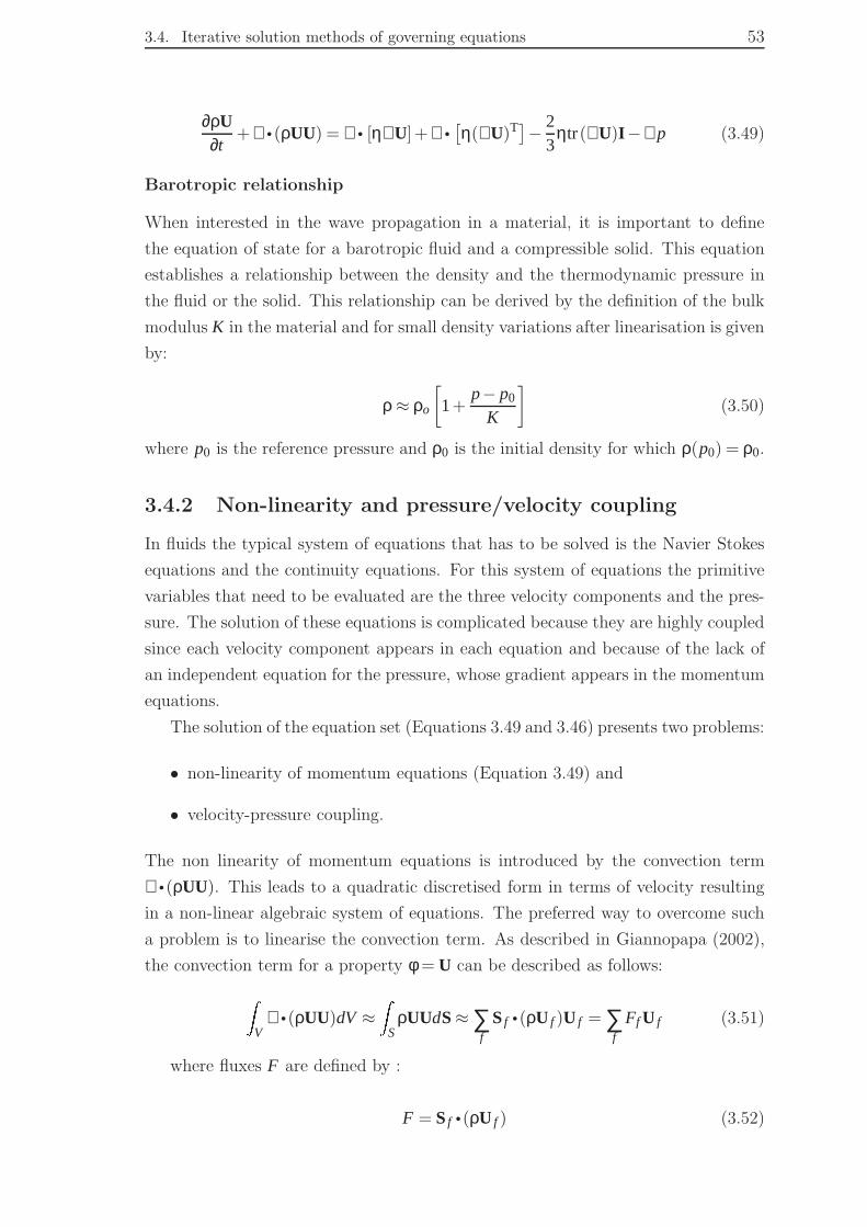
3.4. Iterative solution methods of governing equations 53
∂ρU∂t
+∇ • (ρUU) = ∇ • [η∇U]+∇ •[η(∇U)T]− 2
3ηtr(∇U)I−∇p (3.49)
Barotropic relationship
When interested in the wave propagation in a material, it is important to define
the equation of state for a barotropic fluid and a compressible solid. This equation
establishes a relationship between the density and the thermodynamic pressure in
the fluid or the solid. This relationship can be derived by the definition of the bulk
modulus K in the material and for small density variations after linearisation is given
by:
ρ ≈ ρo
[1+
p− p0
K
](3.50)
where p0 is the reference pressure and ρ0 is the initial density for which ρ(p0) = ρ0.
3.4.2 Non-linearity and pressure/velocity coupling
In fluids the typical system of equations that has to be solved is the Navier Stokes
equations and the continuity equations. For this system of equations the primitive
variables that need to be evaluated are the three velocity components and the pres-
sure. The solution of these equations is complicated because they are highly coupled
since each velocity component appears in each equation and because of the lack of
an independent equation for the pressure, whose gradient appears in the momentum
equations.
The solution of the equation set (Equations 3.49 and 3.46) presents two problems:
• non-linearity of momentum equations (Equation 3.49) and
• velocity-pressure coupling.
The non linearity of momentum equations is introduced by the convection term
∇ •(ρUU). This leads to a quadratic discretised form in terms of velocity resulting
in a non-linear algebraic system of equations. The preferred way to overcome such
a problem is to linearise the convection term. As described in Giannopapa (2002),
the convection term for a property φ = U can be described as follows:ZV
∇ •(ρUU)dV ≈Z
SρUUdS ≈ ∑
f
S f •(ρU f )U f = ∑f
Ff U f (3.51)
where fluxes F are defined by :
F = S f •(ρU f ) (3.52)

54 Chapter 3. Numerical solution method
The convection term can be linearised by treating only the U f term in Equation
3.51 implicitly and using the existing fluxes calculated by the previous time step. It
is important that the fluxes satisfy the continuity equation (Equation3.46).
The non-linearities in the system of equations and the velocity-pressure coupling
can be treated by adopting an iterative solution strategy.
The SIMPLE algorithm (Patankar and Spalding, 1972) or its revised versions
like: SIMPLER (Patankar, 1980) and SIMPLEC (Doormal et al., 1987) using
a staggered grid are the most commonly adopted algorithms used to handle the
velocity-pressure coupling in steady state problems. For transient flow the SIMPLE
algorithm is not very suitable since it does not converge rapidly and its performance
depends greatly on the size of the time step. The PISO algorithm, introduced by Issa
(1986), is the most suitable for transient problems. The algorithm was initially pro-
posed for non-iterative solution of incompressible Navier-Stokes system of equations
using a staggered grid and it has been successfully adopted for iterative methods.
Generalisation to compressible and transonic flows can be found in Demirdzic and
Z.Lilek (1993). This algorithm is used in the present study as well; to the best of
the author’s knowledge it has never been used before for solving the solid solutions.
The PISO algorithm involves one predictor step and two corrector steps and may
be seen as an extention of SIMPLE with a further corrector step. PISO does not
necessarily require iterations within a time level so it is less expensive than SIMPLE.
In Section 3.4.3 the pressure equation for compressible fluids is derived and in
Section 3.4.4 the PISO algorithm is presented.
3.4.3 Derivation of pressure equation
As mentioned above, one of the complexities in the solution of the Navier-Stokes and
continuity equations is the lack of an independent equation for pressure. Before pro-
ceeding in the derivation of a pressure equation, certain things should be mentioned
about the system of equations. The continuity equation does not have a dominant
variable in incompressible flows and it acts as a kinematic constraint on the velocity
field. Therefore one way to overcome this is to construct a pressure field so as to
guarantee the satisfaction of the continuity equation. Based on this assumption, the
pressure equation can be derived, both for incompressible and compressible flows.
Let us consider the momentum equation (Equation 3.49). If both velocity and
pressure are defined at the cell centre, a periodic non-uniform pressure field with
period 2∆x will act as a uniform field in the discretised momentum equations, in
which only the phase values appear. However, such a pressure field is non-physical.
Typically a staggered grid is adopted to overcome this problem. This method is diffi-
cult to extend to unstructured meshes, therefore the Rie-Chow interpolation method
(Rhie and Chow, 1982) that can detect and correct such non-uniform pressure fields

3.4. Iterative solution methods of governing equations 55
has been adopted. All dependent variables are stored at the cell centre using one
control volume, for which the face values of velocities have been interpolated using
the Rie-Chow interpolation method.
So the semi-descretised form of the momentum equation is:
αPUP +∑f
αKUK = S(U)−∇p (3.53)
where U, p are the values from the present time step; αP are the diagonal elements
of the coefficient matrix; αK are the off-diagonal elements associated with the cell
neighbours K; S(U) is the source term containing all the terms that are explicitly
computed (for example see Equation 3.41). An iterative method is used to update
S(U) at every iteration within a time step, so at convergence all terms are calculated
at the new time step.
This form is semi-descritised because the term ∇p is not discretised It should
be noted that this form of the non-linear algebraic equations is identical to the one
derived for solids. Equation 3.53 can be rewritten as:
αPUP = H(U)−∇p (3.54)
where
H(U) = −∑f
αKUK +S(U) (3.55)
So, the H(U) contains the diffusion, convection and temporal terms associated
with cell neighbours as well as the source term calculated explicitly, except from
pressure gradient.
Equation 3.54 can be solved for UP, giving:
UP =H(U)
αP− 1
αP∇p (3.56)
Now let us consider the barotropic relationship (Equation 3.50). Using ψ to
denote ρ0/K:
ρ = ρ0+ψ(p− p0) (3.57)
Substituting Equation 3.56 and Equation 3.57 into the continuity equation (Equa-
tion 3.46) and assuming that K,ρ0, p0 are constant in time and space, the equation
for pressure (that substitutes the continuity equation) can be obtained:
∂ψp∂t︸︷︷︸
implicit
+∇ •
[(ρ0−ψp0)
H(U)
αP
]+∇ •
[ψp
H(U)
αP
]
︸ ︷︷ ︸explicit
−∇ •
[ρ
αP∇p
]
︸ ︷︷ ︸implicit
= 0 (3.58)

56 Chapter 3. Numerical solution method
The first and the fourth term of the equation are implicit, whereas the second
and third are explicit.
To summarise the final form of the system of Navier-Stokes equations for a
compressible fluid is Equation 3.54 and 3.58.
3.4.4 Velocity-Pressure coupling algorithms
The system of equations (3.54 and 3.58), as already mentioned in Section 3.4.2 , is
highly coupled. There are two options for solving this system of equations: using a
direct solver or using an iterative solver.
The direct (or simultaneous) solver, solves the system of equations containing
all dependent variables (i.e. velocity and pressure) simultaneously over the whole
solution domain. In this method, all equations are considered as part of a single
matrix. The solution of a coupled system of equations is a generalisation of the
method used for a single equation. When the computational grid is fine and the
number of equations is large, this solution method is computationally very expensive
in terms of memory requirement and is very slow.
The option of a segregated iterative approach is more appealing. It is based on
the idea of solving a decoupled system for each independent variable, by temporarily
treating all the other variables as known (initially guessing them or taking the values
obtained from the previous iteration or time step). The equations are solved in turn
iteratively until convergence i.e. all equations are satisfied within each time step.
The PISO algorithm uses such an approach for velocity-pressure coupling. The
system of equations is solved using the Biconjugate Gradient method (Hageman
and Young, 1981).
PISO (Pressure Implicit with Splitting of Operators)
The PISO algorithm was initially developed by Issa (1986) for non-iterative com-
putation of incompressible flows using a staggered grid. It was later extended by
Demirdzic and Z.Lilek (1993) for non-iterative computation of compressible and
transonic flows. PISO has been adopted successfully for the iterative segregated
solution for the Navier-Stokes system of equations and can be implemented to a col-
located grid arrangment, with the Rhie-Chow face interpolation method (Rhie and
Chow, 1982). When the algorithm was first published, it was solving for pressure
corrections. In the present implementation, the algorithm is used to solve directly
for pressure rather than its corrections. The flow chart of the PISO algorithm im-
plemented for the present study can be seen in Figure 3.5.
The PISO algorithm can be described as follows:
• STEP1. Momentum predictor: Momentum equation (3.53) is solved in order
to obtain the predicted values for the velocity U∗ field at the new time step.
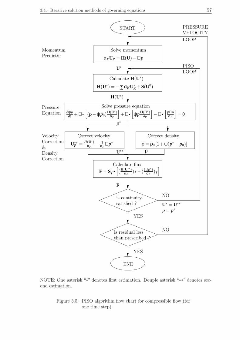
3.4. Iterative solution methods of governing equations 57
END
PressureEquation
VELOCITYPRESSURE
PISOLOOP
START
Calculate flux
Correct velocity
Solve pressure equation
Calculate H(U∗)
Solve momentum
αPUP = H(U)−∇p
YES
YES
VelocityCorrection
F
U∗
U∗∗
p∗
H(U∗)
NO
NO
Momentum
U∗ = U∗∗
p = p∗
Predictor
∂ψp∂t +∇ •
[(ρ−ψp0)
H(U∗)αP
]+∇ •
[ψpH(U∗)
aP
]−∇ •
[ρ∇pαP
]= 0
DensityCorrection
&ρ
LOOP
satisfied ?is continuity
is residual lessthan prescribed ?
Correct density
H(U∗) = −∑αKU∗K +S(U0)
F = S f •[(
H(U∗∗)αP
) f − ((∇p∗)
αP) f
]
U∗∗P =
H(U∗)αP
− 1αP
∇p∗ ρ = ρ0 [1+ψ(p∗− p0)]
NOTE: One asterisk “∗” denotes first estimation. Douple asterisk “∗∗” denotes sec-ond estimation.
Figure 3.5: PISO algorithm flow chart for compressible flow (forone time step).

58 Chapter 3. Numerical solution method
The pressure gradient is treated explicitly using the pressure gradient value
obtained from the previous time step. If it is the first time step, the momentum
is solved with guessed values for pressure obtained from the initial conditions.
This step is performed before entering the PISO loop.
• STEP 2: This is an intermediate step where the term H(U∗) is constructed
using the predicted velocity values using Equation 3.55. This term is going to
be used for the solution of the pressure equation in STEP 3. The values for
the source term are taken from the previous time step or iteration.
• STEP 3. Pressure equation: The pressure equation (3.58) is solved using the
H(U∗) term and the new estimated pressure field p∗is obtained. This pressure
field is not completely correct before convergence is reached after a couple of
iterations in the PISO loop, therefore it is denoted with an asterisk “∗”.
• STEP 4. Velocity correction: Using the new estimated pressure field p∗, the
velocity field is updated U∗∗ (double asterisk “∗∗” denotes second estimation).
The velocity correction is done explicitly using the new pressure field p∗ and
the first velocity prediction in the H(U∗) term. It is assumed that the entire
velocity error comes from the error in the pressure term and the error from
H(U∗) is neglected. Even thought this is not true initially it is corrected since
several PISO loops are executed, so as to make sure that H(U∗) is calculated
using the velocities that satisfy continuity.
• STEP 5. Density correction: The density is also updated using the new esti-
mated pressure field p∗ in order to be used in the next loop.
• STEP 6. Calculate flux: Using the velocity correction H(U∗∗) and the new
pressure field p∗ the new fluxes are evaluated. The fluxes are evaluated by
using the Rhie-Chow interpolation method at the cell fases of the velocities
obtained from Equation 3.56 and substituting it in Equation 3.52. These
fluxes are used in the next time step for the linearisation of the convection
term in the momentum equations. These fluxes should satisfy the continu-
ity equation. Checking if the fluxes satisfy the continuity equation, within a
predefined tolerance, is decided in the decision box for exiting the PISO loop.
If this requirement is not fulfilled, the algorithm returns to STEP 2 and the
process is repeated. So, the PISO loop is from STEP 2 to STEP 6. Since a
new set of fluxes is obtained it would be possible to recalculate the H(U) term.
• STEP 7: This step is again a decision box that checks whether the momentum
equation has been solved within a specified tolerance. If this requirement is
not satisfied, the program returns to STEP 1 and repeats the loop. If it is
fulfilled, the program moves to the next time step.

3.5. Investigation of boundary conditions for fluids 59
So, the PISO algorithm for compressible fluids consists of one implicit momentum
predictor (STEP 1) followed by a series of pressure solutions (STEP 3), explicit ve-
locity (STEP4) and density corrections (STEP 5). This series of corrections (STEP
3, 4, 5) is repeated until convergence is reached within the predefined tolerance.
3.5 Investigation of boundary conditions for flu-
ids
In order to derive a unique solution to any system of PDEs, a set of conditions needs
to be specified at the boundary of the computational domain.
These boundary values have either to be known or be expressed as a combina-
tion of internal values and boundary data. These approximations have to be derived
by internal value differences or extrapolations. Generally as mentioned in (Gi-
annopapa, 2002) the boundary condition types for any property can be: fixed value
(or Dirichlet); fixed gradient (or Neumann); or mixed boundary condition, which is
a linear combination of the other two.
In this and the next subsections, boundary condition types and their derivations
for velocity and pressure for the Navier-Stokes equations for compressible and in-
compressible flows is examined. The main focus is the pressure boundary condition.
In order to specify the correct condition needed for the solution of the Navier-
Stokes equation for compressible and incompressible flow, the different roles of pres-
sure in these equations should be considered and therefore are discussed below.
Incompressible flow
In incompressible flow, there is no equation of state. Therefore, pressure is not a
thermodynamic variable. The pressure propagates at an infinite speed in order to
establish an incompressible flow and its role is to force the time varying velocity
field to remain divergence free at all times.
In terms of computation, the Navier-Stokes equations are solved and an initial
predicted velocity field is calculated. This velocity field is corrected using the pres-
sure values derived by the solution of a Poison pressure equation and should be as
close as possible to the initial predicted ones. It can be proved (Ferziger and Peric,
1996) that the pressure can be seen as a Lagrange multiplier used to minimise the
functional
R=12
ZV
[U∗∗(r)−U∗(r)]2dV (3.59)
where r is the position vector, U∗ is the original velocity field and U∗∗ is the
corrected velocity field.

60 Chapter 3. Numerical solution method
For the solution of the Navier-Stokes equations, boundary conditions have to be
specified for both velocity and pressure. It is typical to apply a fixed value (i.e.
Dirichlet) boundary condition for the velocity at the boundary. The Navier-Stokes
equations require that all the components of the velocity vector should be specified
on the boundary.
For a wall, no-slip boundary conditions are specified. This means that the ve-
locity of the fluid is equal to the velocity of the wall. It should also be mentioned
that the normal viscous stress is zero at the wall due to the continuity equation.
For a symmetry plane, the velocity component parallel to the surface of the sym-
metry plane has zero normal gradient. A gradient (usually zero) of all quantities is
specified on the outflow surface.
It is important to point out that the Navier-Stokes equations require no a priori
knowledge of the boundary conditions of pressure. The velocity boundary conditions
applied to the momentum equations are sufficient to allow the determination of body
velocity and pressure. Since only the first time derivative is present in Equation 3.47,
it is sufficient to prescribe the initial velocity field at t = 0. Of course this velocity
field must satisfy the incompressibility condition (O.Ladyshenkaya, 1998). The
boundary condition for pressure though, is one that has received the most debate in
the literature.
Orszag and Israeli (1974) conclude that either the normal or the tangential com-
ponents of the (vector) momentum Navier-Stokes equation is permissible as a bound-
ary condition for the pressure Poison equation. This raises a serious dilemma, since
the former leads directly to a fixed gradient (or Neuman) boundary condition and
the later indirectly to a fixed value (or Dirichlet) boundary condition.
Moin and Kim (1980) stated that the fixed value and fixed gradient problems for
pressure, if properly derived form a well-posed Navier-Stokes problem, will have the
same solution at least for t > 0. According to Gustafsson and Sundstrom (1978) the
boundary conditions for pressure equation are obtained by applying the momentum
equation (normal component) and the continuity equation at the wall.
Gresho and Sani (1987) agree with their general idea. Therefore, they rederive
the equations again and they answer to the question of Gustafsson and Sundstrom
(1978) paper by stating that the divergence-free condition is of the utmost impor-
tance for theoretical and computational fluid dynamics.
Gresho and Sani (1987) demonstrate that for the solution of the pressure Poi-
son equation, the fixed value (or Dirichlet) boundary condition for pressure is only
appropriate for t > 0 and it often does not apply for t = 0. Only the fixed gradient
(or Neumann) BC is always appropriate and provides a unique solution for t ≥ 0.
Any consistent discrete approximation of the original Navier-Stokes equations con-
tains a built-in boundary condition for the discrete pressure Poison equation that is
fixed gradient (or Neuman) boundary condition for t ≥ 0. This does not obviously

3.5. Investigation of boundary conditions for fluids 61
satisfy the fixed value (or Dirichlet) boundary condition, however. The converged
numerical solution will also satisfy the Dirichlet boundary condition, but for t > 0,
complementing the conclusion of Moin and Kim (1980).
Let us consider the momentum equation
∂U∂t
+∇ •(UU)−∇ •(η∇U) = −∇p (3.60)
where η is the kinematic viscosity and the continuity equation for incompressible
flow:
∇ •U = 0 (3.61)
Gresho and Sani (1987) derive two pressure Poison equations and therefore two
equations for fixed gradient (or Neumann) boundary condition. One is the simplified
form and is derived by including the continuity equation into the momentum. The
other one is the consistent form where continuity is not included in momentum and
from which we can derive the following boundary condition equation.
n •∇p = n • (η∇U−U∇U)− ∂U∂t
(3.62)
The conclusion from their paper is that the correct boundary condition is the
fixed gradient (or Neumann) and is obtained by applying the normal component of
the momentum equation at the boundary. It should be mentioned that the solution
for pressure computed using Equation 3.62 also satisfies the fixed value (or Dirichlet)
boundary condition, which emerges by projecting the equation of motion onto a tan-
gential vector and then integrating it with respect to the tangential arc length.The
equivalent fixed gradient (or Neumann) boundary condition for compressible fluids
will be derived and presented in Section 3.6 and will be tested in Chapter 4.
Deng and Tang (2002) solve the incompressible Navier-Stokes equations and they
are also concerned with finding the correct boundary conditions for the solution of
these equations. In their solution approach they use the SIMPLE algorithm with
pressure corrector for the velocity and pressure coupling. From their investigation
they conclude that when the velocity boundary conditions are Dirichlet, the bound-
ary conditions for the pressure correction should be Neumann; but when the velocity
boundary conditions are Neumann, the boundary conditions for the pressure correc-
tion should be Dirichlet.
Compressible flow
For compressible flow, the boundary conditions are different from the ones used for
incompressible equations, since the compressible equations are hyperbolic in charac-
ter. A compressible fluid can support sound and shock waves and it is not surprising

62 Chapter 3. Numerical solution method
that these equations have essentially hyperbolic character. Hyperbolic flows have
characteristics that are real and distinct. Information propagates in two sets of
directions. The equations for viscous-compressible flow are still more complicated.
Their characteristics are a mixture of elements that do not fit well into the classifi-
cation scheme and numerical methods for them are difficult to construct. Therefore
special care should be taken in the specification of the boundary conditions.
According to Ferziger and Peric (1996) for incompressible flow, the following
boundary conditions can be applied:
• Inflow boundaries: prescribed velocity and temperature on inflow boundaries.
• Symmetry planes: zero gradient normal to the boundary for all scalar quanti-
ties and the velocity component parallel to the surface on a symmetry plane;
zero velocity normal to such a surface.
• Solid surface: non-slip (zero relative velocity) conditions, zero normal stress
and prescribed temperature or heat flux on a solid surface.
• Outflow boundaries: rescribed gradient (usually zero) of all quantities on an
outflow surface.
These boundary conditions also hold for compressible flow and are treated in the
same way as in incompressible flows. However, in compressible flow there are further
boundary conditions.
• prescribed total pressure (at the inflow)
• prescribed total temperature (at the inflow)
• prescribed static pressure (at the outflow)
• at a supersonic outflow boundary, zero gradient of all quantities are usually
specified.
In order to define the total pressure at the inflow, the equation of state is usually
used and the direction of the flow must be specified. It should be mentioned that
the implementation of Ferziger and Peric (1996) is for pressure correction. The
static pressure specified at the outflow boundary is again implemented by taking
into consideration pressure and velocity correction at the boundary.
For computational reasons an artificial boundary is usually introduced. For
purely hyperbolic problems, it is well known that enforcing these boundary con-
ditions through the characteristic variables leads to a stable approximation however
for dissipative wave problems this procedure is considerably more complicated.
Hesthaven and Gottlieb (1996) and Hesthaven (1997) are interested in dissipa-
tive, wave dominated problems and they derive stable open boundary conditions

3.6. Boundary condition for solids for the unified solution method 63
ensuring that the continuous problem is well-posed. The proposed boundary con-
ditions are applied through the penalty procedure. Once the form of the boundary
conditions is known, the way to implement them is to solve the equation in the
interior points of the computational domain and then to enforce the boundary con-
ditions at the boundary points. However, this approach does not take into account
the fact that the equation should be satisfied arbitrarily close to the open boundary.
Therefore, the penalty method is used to enforce the boundary condition, as well as
taking into account the equation at the boundary.
Gustafsson and Sundstrom (1978) and Olivier and Sundstrom (1978) use the
energy method to obtain boundary conditions for the linearised constant coeffi-
cient Navier-Stokes equations in the primitive variable formulation. Dutt (1988)
introduced an entropy function which allowed him to derive boundary conditions
for non-linear problems ensuring that the solution remains bounded in an entropy
norm.
3.6 Boundary condition for solids for the unified
solution method
In order to derive a unique solution for the equations of interest, a set of condi-
tions needs to be specified at the boundary of the solution domain. The boundary
condition investigation in Section 3.4 has guided the choice of the boundary condi-
tions for solids that were used for the solution of the mathematical models described
in Chapter 2 and are described in detail here. Every time the momentum equa-
tion (Equation 3.36, 3.39 and 3.40) is solved, the values of displacement (for
Equation 3.36) or velocity (for Equation 3.39 or 3.40) need to be updated at the
boundary.
The solution of momentum and pressure at the interior point and the satisfaction
of boundary conditions is achieved through an iterative process, as already explained.
This process is repeated until convergence is reached and the equations are solved
to a specified residual. In the first couple of time steps, it takes more iterations to
reach the required residual. In order to speed up the process, the program moves to
the next time step when the number of iterations has reached 50. This number was
specified by trial and error. In the subsequent time steps, convergence is achieved
within usually 10-15 iterations.
Since, the deformations concerned in the present study are very small the convec-
tion term ∇ •(ρUU) on the left hand side of the momentum Equation 2.2 is negligible.
So, momentum equation can be rewritten as:
∂ρU∂t
= ∇ •σ (3.63)

64 Chapter 3. Numerical solution method
3.6.1 Boundary conditions for the displacement formulation
The appropriate boundary condition for the displacement can be obtained by ap-
plying the force balance at the boundary. This relationship can be described by:
n •σ = t−npext (3.64)
where pext is the external pressure applied at the boundary and t is the external
traction.
Fixed gradient using force balance This boundary condition can be ob-
tained by substituting stress from Equation 2.13 in Equation 3.64 and solving for
n •∇D. The resulting equation is afterwards reformulated in order to be consistent
with the form of the momentum equation as presented in Equation 3.36. The final
form of the displacement gradient normal to the boundary is:
n •∇D =t−npext−n •
[(−µ−λ)∇D+µ∇DT
]−nλtr (∇D)
(2µ+λ)(3.65)
Fixed value using force balance This fixed normal gradient boundary con-
dition can be substituted to:
nb • (∇D)b =Db−DN
|dN|(3.66)
Therefore, from Equation 3.65 and 3.66 the fixed value boundary condition ex-
pression for the displacement can be obtained as
Db = DN+ | dN | t−npext−n •[(−µ−λ)∇D+µ∇DT
]−nλtr(∇D)
(2µ+λ)
3.6.2 Boundary conditions for the velocity formulation
The boundary condition types that were tried for velocity were fixed value and fixed
gradient and were obtained by applying force balance at the boundary (Equation
3.64).
Fixed gradient using force balance This boundary condition is obtained
by substituting the stress from Equation 2.17 in Equation 3.64 and solving for n •∇U.
The resulting equation is afterwards reformulated in order to be consistent with the
form of the momentum equation presented in Equation 3.39. The final form of the
velocity gradient normal to the boundary is:
n •∇U =2∆t [t−npext−nΣ+]+n •
[(−µ−λ)∇U+µ∇UT
]−nλtr(∇U)
(2µ+λ)(3.67)

3.6. Boundary condition for solids for the unified solution method 65
where pext is the external pressure applied at the boundary and t is the external
traction.
Fixed value using force balance The fixed value boundary condition is
obtained from the fixed gradient by simply substituting the face normal gradient to:
nb • (∇U)b =Ub−UN
|dN|(3.68)
Therefore, from Equation 3.67 and 3.68, we can derive the fixed value boundary
condition expression for the velocity as
Ub = UN+ | dN |2∆t [t−npext−nΣ+]+n •
[(−µ−λ)∇U+µ∇UT
]−nλtr(∇U)
(2µ+λ)(3.69)
3.6.3 Boundary conditions for the velocity-pressure formu-
lation
There are two ways that the velocity/pressure formulation is solved: pressure explicit
and pressure implicit. When the pressure is specified explicitly, no partial differential
equation is solved so no boundary condition is needed. The pressure p is linearly
extrapolated from the internal field to the boundary. Only in the case where the
pressure is solved implicitly is there a need to specify an appropriate condition for
the solution of the pressure at the boundary.
3.6.3.1 Boundary conditions for velocity
Fixed gradient using force balance The same way it was obtained in the
displacement formulation, this boundary condition is obtained by substituting stress
from Equation 2.21 in Equation 3.64 and solving for n •∇U. The resulting equation is
afterwards reformulated in order to be consistent with the expression of momentum
presented in Equation 3.40 (or 3.41). The final form of the velocity gradient at the
boundary is:
n •∇U =2∆t [t−npext−n(devΣ+)+np]+n •
[(−µ−λ)∇U+µ∇UT
]+n2
3µtr(∇U)
(2µ+λ)(3.70)
Fixed value using force balance The fixed value boundary condition for
the velocity is obtained as in the previous section by simply substituting the face
normal gradient. This expression is:

66 Chapter 3. Numerical solution method
Ub =|UN |+dN
2∆t [t−npext−n(devΣ+)+np]+n •
[(−µ−λ)∇U+µ∇UT
]+n2
3µtr(∇U)
(2µ+λ)(3.71)
3.6.3.2 Boundary condition types for pressure
The boundary condition expressions for pressure can be obtained in one of three
ways: from the definition of pressure or from applying the force balance relation at
the boundary or by projecting the momentum equation at the unit vector normal
to the boundary.
Fixed value using the definition of pressure This boundary condition is
given by
p = p0−K∆t2
tr(∇U+∇U0) (3.72)
where p0 is the old value obtained at the end of the previous time step.
Fixed value using using force balance This boundary condition type used
for the pressure is fixed value and has been derived by applying force balance (Equa-
tion 3.64) at the boundary and solving for pressure, in the same way the equation
for velocity at the boundary was obtained. So, the value of pressure at the boundary
is given by:
p = −t •n+ pext+n •devΣ+ •n−αn •
[∇U+(∇U)T− 2
3tr(∇U)I
]•n (3.73)
where is α = ∆t2 .
Fixed gradient using momentum This boundary condition type is fixed
gradient and an equation for its value is derived by projecting the momentum equa-
tion at the unit vector normal to the boundary and solving for n •∇p. So we get:
n •∇p =∆t2
n •
[∇ • [µ∇U]+∇ •
[µ(∇U)T]− 2
3µ∇ • [tr∇UI]
]+n •∇ •devΣ+− ∂ρU
∂t(3.74)
This formulation has been derived according to the paper of Gresho and Sani
(1987) but for a compressible material.

3.6. Boundary condition for solids for the unified solution method 67
Fixed value using momentum This boundary condition is obtained from
the gradient boundary condition (Equation 3.74) by simply substituting the face
normal gradient at
nb • (∇p)b =pb− pN
|dN|(3.75)
Therefore, from Equation 3.74 and 3.75 we can derive the fixed value boundary
condition expression for the displacement as
pb = pN+ | dN | ∆t2
n •
[∇ • [µ∇U]+∇ •
[µ(∇U)T]− 2
3µ∇ • [tr∇UI]
]+n •∇ •devΣ+− ∂ρU
∂t(3.76)
3.6.4 Optimal choice of boundary conditions
In this section the type of boundary conditions that give the best results and are
used for obtaining the results in the following chapter was presented. For the stan-
dard displacement formulation, a fixed gradient boundary conditions was used which
was obtained by applying the force balance relation at the boundary (Equation
3.65). For the velocity formulation a fixed gradient boundary condition was used
and was obtained again using the force balance relation (Equation 3.67). In the
velocity-pressure explicit formulation there is no need to specify a separate bound-
ary condition for the pressure at the boundary. The pressure is linearly extrapolated
from the internal fields to the boundary. For the velocity a fixed gradient boundary
condition is applied and the expression is obtained again from the force balance
relation (Equation 3.70). In the velocity-pressure implicit formulation a fixed value
condition is applied for the pressure. The expression is obtained by projecting the
momentum equation to the unit vector normal to the boundary and solving for the
pressure gradient n •∇p. The value of pressure at the boundary is then obtained
from the gradient with linear interpolation from the internal values (Equation 3.76).
For the velocity, again a fixed gradient boundary condition is chosen by applying
force balance (Equation 3.70), as it was found to have worked quite well for the
other cases. It should be noted that the boundary condition type for velocity and
pressure when using an implicit iterative solution method should be fully reversible
i.e. when a fixed gradient boundary condition is used for the velocity a fixed value
boundary condition is used for pressure and vice versa (Deng and Tang, 2002).

68 Chapter 3. Numerical solution method
Discrete grid pointsShortest resolvable wave with highestresolvable wave number
∆x
L=2∆x
Figure 3.6: Shortest resolvable wave.
3.7 Stability Analysis
A number of methods exist to investigate the stability limits of a finite difference
scheme. One such a method is the Fourier or Von Neuman analysis (Mattheij
et al., 2005; Hirsch, 1988; Anderson et al., 1984; Abbott and Basco, 1989). This
method will be described here and will be used to investigate the stability of the
numerical method for the solution of displacement equations used in the standard
stress analysis and the velocity equation developed and used in this project.
Suppose that the solution of any finite difference scheme at point j at time level
n can be written as a Fourier series in complex, exponential form:
Dnj =
kk
∑k=1
bnkeiα j (3.77)
or alternatively
D(x, t) =kk
∑k=1
bk(t)eikmx (3.78)
The index n is the time level index; j is the grid point index; k= 1,2,3...,kk is the
wave number index; i is the imaginary unit; bnk is the Fourier coefficient (amplitude)
for wave number k at time level n; km is the wave number index and is equal to
km= 2πL k, where L is the wave length; and α is the dimensionless wave number
which is equal to α = km∆x = 2πL k∆x = k2π
N (0 ≤ α ≤ π), were N is the number of
grid intervals over one wavelength. In Figure 3.6 the graphical representation of the
shortest resolvable wave with the highest resolvable wave number can be seen. It
is apparent that the number of grid integrals in one wavelength is ∞ > N ≥ 2. It is
also obvious that x j = j∆x.
The Fourier analysis method determines how each Fourier coefficient behaves

3.7. Stability Analysis 69
(grows, decays, or stays constant) in time for any wave number index k. For example
for k = 1
Dnj = bn
1eiα j (3.79)
is a solution of the finite difference scheme. Note that n is not a power but a
time index. This equation can be used to obtain the solution at any point in space
and time. For example at the n+1 time instance at location j:
Dn+1j = bn+1eiα j (3.80)
and at j +1 point at the n-th instance it gives:
Dnj+1 = bneiα( j+1) (3.81)
where the wave number index k is dropped.
When the terms from the Equations 3.80 and 3.81 and the corresponding ones
from every other time instant and point that appear in the finite difference equation
are substituted into the discretised equation, the resulting expressions are rearranged
to take the form shown by
bn+1 = Gbn (3.82)
where G is called the amplification or growth factor.
For a particular numerical method, the amplification factor depends upon the
mesh size and the wave number or frequency. For hyperbolic problems, like the ones
concerned in this thesis, G depends on the Courant number, Co = c∆t∆x, where c is the
velocity of the propagating wave. To have a stable FD scheme, the Fourier coefficient
must not grow without bound i.e. the magnitude of the Fourier coefficient of each
and every wave number should not increase in time. So the stability condition is
given by
|G| ≤ 1 (3.83)
The stability analysis can also be used to determine the amplitude and the phase
accuracy for all possible α (or alternative, for all grid intervals per wave length, N).
It is assumed that for a given equation the amplification factor has been obtained
G(α,Co). This can be used to calculate the amplitude of the response module |G|and
the phase response Q. The celerity ratio Q is defined as shown in Equation 3.84.
Q =−arg(G(α))
Coα=
−tan−1(
Im(G)Re(G)
)
Coα(3.84)

70 Chapter 3. Numerical solution method
t
n
n-1
n-2
j j+1j-1
∆x
∆t
Figure 3.7: Stencil for the 1D hyperbolic finite difference equation(3.90).
3.7.1 Wave equation (1D)
The standard stress analysis equation in 1D with the assumption of constant density
ρ is a hyperbolic equation known as the wave equation and can be written as:
ρ∂2Dx
∂t2 = (2µ+λ)∂2Dx
∂x2 , tε [0,∞) , xε [0,L] (3.85)
The wave velocity for plain strain is given by Equation 3.86.
c1 =
√2µ+λ
ρ=
√1−ν
(1+ν)(1−2ν)
ϒρ
(3.86)
Longitudinal waves in uniform bars with uniform cross section are given by Equa-
tion 3.87, where c=√
ϒρ . The wave velocity c is lower than the wave velocity c1 and
their ratio depends on ν. For example, for ν = 0.3, the ratio is c1/c = 1.16.
∂2D∂t2 = c2∂2D
∂x2 (3.87)
Using the first order Euler implicit difference approximation to approximate the
second order time derivative ∂2D∂t2 and the second order central approximation for the
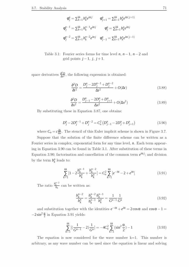
3.7. Stability Analysis 71
φnj = ∑kk
k=1bnkeiα j φn
j+1 = ∑kkk=1bn
keiα( j+1)
φn−1j = ∑kk
k=1bn−1k eiα j φn
j = ∑kkk=1bn
keiα j
φn−2j = ∑kk
k=1bn−2k eiα j φn
j−1 = ∑kkk=1bn
keiα( j−1)
Table 3.1: Fourier series forms for time level n, n−1, n−2 andgrid points j −1, j, j +1.
space derivatives ∂2D∂x2 , the following expression is obtained:
∂2D∂t2 =
Dnj −2Dn−1
j +Dn−2j
∆t2 +O(∆t) (3.88)
∂2D∂x2 =
Dnj−1−2Dn
j +Dnj+1
∆x2 +O(∆x2) (3.89)
By substituting these in Equation 3.87, one obtains:
Dnj −2Dn−1
j +Dn−2j = C2
o
(Dn
j−1−2Dnj +Dn
j+1
)(3.90)
where Co = c∆t∆x. The stencil of this Euler implicit scheme is shown in Figure 3.7.
Suppose that the solution of the finite difference scheme can be written as a
Fourier series in complex, exponential form for any time level, n. Each term appear-
ing in Equation 3.90 can be found in Table 3.1. After substitution of these terms in
Equation 3.90; factorisation and cancellation of the common term eiα j ; and division
by the term bnk leads to:
kk
∑k=1
[1−2bn−1
k
bnk
+bn−2
k
bnk
] = C2o
kk
∑k=1
[e−iα −2+eiα] (3.91)
The ratiobn−2
kbk
can be written as:
bn−2k
bnk
=bn−2
k
bn−1k
bn−1k
bnk
=1
Gn−1
1Gn (3.92)
and substitution together with the identities e−iα +eiα = 2cosα and cosα−1 =
−2sin2 α2 in Equation 3.91 yields:
kk
∑k=1
[(1
Gn−1 −2)1
Gn ] = −4C2o
kk
∑k=1
(sin2 α2)−1 (3.93)
The equation is now considered for the wave number k=1. This number is
arbitrary, as any wave number can be used since the equation is linear and solving

72 Chapter 3. Numerical solution method
for the amplification factor Equation 3.94 is obtained, where α = 2π/N and Nε [2,∞).
Gn =2− 1
Gn−1
1+4C2o sin2 α
2
(3.94)
In Equation 3.91 for a single mode a solution of the form bn = λn can be tried,
where in b the use of n is time index and in λ power. After substitution the charac-
teristic or dispersion Equation 3.95 is obtained. It can be seen that time level is not
included so assuming that the amplification factor between consecutive time steps
is the same Gn = Gn−1 = G = λ gives .
(1+4C2o sin2 α
2)λ2−2λ+1 = 0 (3.95)
This equation has two solutions. Therefore two amplification factors exist that
must satisfy the stability condition (Equation 3.83), although the exact solution has
a single value of the amplification. The solution with the positive sign corresponds
to the physical solution, whereas the one with the negative sign propagates in the
other direction. The solutions of Equation 3.95 are:
G =1
1± i2Cosinα2
(3.96)
The amplitude and phase portrait of G at different Co numbers Co = 14, 1
2, 34, 1, 5
4
are shown in Figure 3.8.
The scheme used for the discretisation of the Equation 3.85 is unconditionally
stable for all Co, but it is dissipative. This means that the amplitude of the wave will
suffer an attenuation of some magnitude at each time step. This numerical damping
is well known as numerical viscosity (or dissipation). The numerical dissipation gets
smaller by reducing ∆x (or increasing N). From the phase portrait it can be seen
that there is a phase shift of the travelling wave which can be improved by increasing
the number of grid points per wave length N.
3.7.2 Velocity formulation for linear elastic Hookean solid
(1D)
The equation of the velocity formulation in 1D with the assumption of constant
density ρ can be written in the form bellow, where m= 1, 2, ..., n is the time step
index.
ρ∂Ux
∂t=
∆t2
(2µ+λ)n
∑m=1
[∂2Um
x
∂x2 +∂2Um−1
x
∂x2 ] , tε [0,∞) , xε [0,L] (3.97)

3.7. Stability Analysis 73
0 5 10 15 20 250.2
0.3
0.4
0.5
0.6
0.7
0.8
0.9
1
N
|G|
Co=1/4Co=1/2Co=3/4Co=1Co=5/4Co=2
(a) Amplitude portrait
0 5 10 15 20 250.2
0.3
0.4
0.5
0.6
0.7
0.8
0.9
1
N
Q
Co=1/4Co=1/2Co=3/4Co=1Co=5/4Co=2
(b) Phase portrait
Figure 3.8: Accuracy portrait of the amplification factor G for the1D hyperbolic equation (3.96).

74 Chapter 3. Numerical solution method
By substituting the wave velocity c =√
ϒ/ρ in Equation 3.97 the 1D velocity for-
mulation can be written as Equation 3.98.
∂Ux
∂t=
∆t2
c2n
∑m=1
[∂2Um
x
∂x2 +∂2Um−1
x
∂x2 ] , tε [0,∞) , xε [0,L] (3.98)
The above expression is equivalent to the following system of first order ordinary
differential equations
∂Ux∂t = c2∂2Dx
∂x2 (3.99)
∂Dx
∂t= Ux (3.100)
The velocity formulation expression that contains the summation (Equation 3.98)
is not in a form suitable for perform a stability analysis. Thus, using the main
principle of the von-Neuman analysis and extending it to a system of equations,
the stability analysis can be performed on the system of Equations 3.99 and 3.100
instead.
Using the first order Euler implicit difference approximation to approximate the
first order time derivative ∂U∂t and the second order central approximation for space
derivatives ∂2D∂x2 for Equation 3.99 the following is obtained:
∂U∂t
=Un
j −Un−1j
∆t+O(∆t) (3.101)
∂2D∂x2 =
Dnj−1−2Dn
j +Dnj+1
∆x2 +O(∆x2) (3.102)
The trapezoidal rule is used for the approximation of the integral in Equation
3.100 (as described in Section 2.3.2) , thus
Dnj = Dn−1
j +∆t2
(Un
j +Un−1j
)(3.103)
Thus, Equation 3.98 can be equivalently written as:
Unj −Un−1
j
∆t= c2
(Dn−1
j+1 −2Dn−1j +Dn−1
j−1
∆x2 +∆t2
Unj+1−2Un
j +Unj−1+Un−1
j+1 −2Un−1j +Un−1
j−1
∆x2
)
(3.104)
The stencil of this Equation can be found in Figure 3.9. The treatment of the
spatial term is equivalent to theta-method for θ = 1/2. Thus the stencil is that of
the theta-method with θ = 1/2. The theta methods are linear combinations of the
explicit and implicit Euler schemes. In such schemes, the parameter θ is used to
optimise the accuracy and/or the stability of a scheme. For θ = 1/2 the scheme
is a Crank-Nicolson scheme and it is unconditionally stable. The theta method

3.7. Stability Analysis 75
t
n
n-1
n-2
j j+1j-1
∆x
∆t
Figure 3.9: Stencil for the 1D system of equations that isequivalent to the 1D velocity formulation.

76 Chapter 3. Numerical solution method
is in general first order accurate in the time and second order accurate in space;
for θ = 1/2 it is also second order accurate in ∆t (Mattheij et al., 2005; Higham,
2000). Thus, it is expected from the stability analysis that the equivalent system
of equations to be unconditionally stable and compared with the wave equation
(Section 3.7.1) to be less dissipative.
The system of Equations 3.99 and 3.100 after substitution of the time and space
approximations and setting ζ = ∆t2 and ξ =
C2o
∆t give:
Dnj −Dn−1
j = ζ(Un
j +Un−1j
)(3.105)
Unj −Un−1
j = ξ(Dn
j−1−2Dnj +Dn
j+1
)(3.106)
Suppose that the solution of any finite difference scheme can be written as a
Fourier series in complex, exponential form for any time level, n. Each term appear-
ing in Equations 3.105 and 3.106 can be found in Table 3.1. After substitution of
these terms in the system of equations, factorisation and cancellation of the common
term eiα j ; and using the identities e−iα + eiα = 2cosα and cosα−1 = 2sin2 α2 , the
following equations can be obtained:
kk
∑k=1
[bnk,D−bn−1
k,D ] = ζkk
∑k=1
[bnk,U +bn−1
k,U ] (3.107)
kk
∑k=1
[bnk,U −bn−1
k,U ] = 4ξkk
∑k=1
[sin2 α2
bnk,D] (3.108)
The second index i.e. D or U in the subscript of the Fourier coefficient is used
to denote the variable that this coefficient belongs to, i.e. displacement and velocity
respectively. For a single mode, for example k = 1, the system of equations can take
the matrix form as:
[bn+1
D
bn+1U
]
= A
[bn
D
bnU
]
(3.109)
where A is the matrix
A =
1−2C2
osin2 a2
1+2C2osin2 a
2
−4C2o
∆t sin2 a2
2
1+2C2osin2 a
2∆t
1+2C2osin2 a
2
11+2C2
osin2 a2
The eigenvalues of the 2x2 matrix A will give the characteristic or dispersion
equation, which reads:
λ2− 2(1−C2o sin2 α
2)
1+2C2o sin2 α
2
λ+1
1−2C2o sin2 α
2
= 0 (3.110)

3.7. Stability Analysis 77
0 5 10 15 20 250.85
0.9
0.95
1
N
|G|
Co=1/4
wave equationvelocity formulation
0 5 10 15 20 250.7
0.8
0.9
1
N
|G|
Co=1/2
wave equationvelocity formulation
0 5 10 15 20 250.4
0.6
0.8
1
N
|G|
Co=3/4
wave equationvelocity formulation
0 5 10 15 20 250.4
0.6
0.8
1
N
|G|
Co=1
wave equationvelocity formulation
0 5 10 15 20 250.2
0.4
0.6
0.8
1
N
|G|
Co=5/4
wave equationvelocity formulation
0 5 10 15 20 250.2
0.4
0.6
0.8
1
N
|G|
Co=2
wave equationvelocity formulation
Figure 3.10: Amplitude portrait of the 1D velocity formulation incomparison with the wave equation (displacementformulation).
Setting ϑ =−2C2o sin2 α
2 in Equation 3.110 and from the solution of the quadratic
equations the two values for the amplification factor G = λ can be obtained. These
values must satisfy the stability condition (Equation 3.83)
λ = G =2
−2−ϑ±√
ϑ(ϑ+8)(3.111)
where α = 2π/N and Nε [2,∞). The solution with the positive sign in Equation
3.111 corresponds to the physical solution, whereas the one with the negative sign
propagates in the other direction.
The accuracy amplitude portraits for different Courant numbers Co = 14, 1
2, 34, 1, 5
4
in comparison with these of the displacement equation are shown in Figure 3.10. The
scheme used for the discretisation of the Equation 3.87 is unconditionally stable for
all Co and the numerical damping is smaller than the scheme used for the wave
equation. Thus this discretisation scheme is more accurate.

78 Chapter 3. Numerical solution method
3.8 Closure
The finite volume method has been applied for the discretisation of the governing
mathematical equations presented in Chapter 2. This method has a long tradition
in computational fluid dynamics. As the reformulated equations for solids have
velocity and pressure as primitive variables, the finite volume method seems to be
the natural choice.
Only the basic principles of the FV method have been presented in this chapter.
Specific attention has been drawn to the discretisation of the Laplacian operator
versus the divergence-gradient operator. The two operators, even though mathe-
matically the same, are discretised differently. Thus, care should be taken when
used as they introduce different discretisation errors.
Practical issues involving the solution procedure with emphasis to the conver-
gence rate have been addressed. The equations have been reformulated to their most
implicit part in order to increase convergence rate according to Jasak and Weller
(2000) paper.
When velocity and pressure are both solved implicitly in the unified formulation
for fluid structure interaction problems, the solution is complicated mainly due to
the fact that there is no independent equation for pressure and each one of the ve-
locity components appears in all equations creating a highly coupled system. The
PISO algorithm has been adopted to solve iteratively the coupled system. A decou-
pled sub-system for each independent variable is solved by temporarily treating all
the other variables as known in an iterative segregated manner. In the present im-
plementation, the PISO algorithm solves for velocity and pressure, rather than their
corrections. The PISO algorithm is typically used for the solution of the Navier-
Stokes equations for fluid and, to the best of the author’s knowledge, it has never
been used before for structural analysis.
In order to derive a unique solution for the momentum equations whether they are
used to solve fluid dynamic problems or solid mechanics problems or fluid-structure
interaction problems, a set of conditions must be specified at the boundary of the
computational domain. The boundary values can either be known or evaluated by
descritising the boundary conditions using the internal cell values.
In order to find the appropriate boundary conditions for solids, a thorough liter-
ature investigation was performed to see what are the most appropriate boundary
conditions for fluids. The conclusion from this investigation was that the choice of
boundary conditions for pressure has received the most intense debate in the litera-
ture. The best choice for deriving an expression for pressure at the boundary is to
solve the momentum equation for the normal component of the pressure gradient.
Based on this, the appropriate boundary conditions were derived for solving the
solids with the new unified solution method that is consistent with a one for fluids.

3.8. Closure 79
For the velocity, a fixed gradient boundary condition can be obtained by applying
the force balance relation at the boundary. For the pressure, a fixed value boundary
expression can be derived by solving for the normal component of the pressure
gradient in the momentum equation and then calculating the pressure value from
the gradient.
In the last part of this chapter, a stability analysis has been presented for the
discretisation of the velocity based formulation in comparison with the equivalent
standard stress analysis formulation for solids. The discretisation scheme for the
new velocity formulation is unconditionally stable for all Courant numbers and is
less dissipative than the one used to discretise the displacement equation. This
means that the solution of the amplitude of the wave will suffer less attenuation at
each time step in comparison with the standard formulation.

80 Chapter 3. Numerical solution method

Chapter 4
Validation of the new formulation
for solids
4.1 Introduction
The new unified formulation with velocity and pressure as primitive variables pre-
sented in Chapter 2 is standard for compressible or incompressible fluid modelling
but is new for solids and therefore, needs to be tested. A beam bending case was
chosen to validate the method. The interest in such a case stems from the need to
use a difficult case that comprises, apart from normal stress, shear stress as well.
The effect of shear is of great importance in wave propagation, so such a case would
be a good validation tool.
4.2 Case Description
A narrow cantilivered beam was considered as shown in Figure 4.1, loaded at its
free end by a concentrated force of such magnitude that the weight of the beam can
be neglected. The material properties of the beam and its dimensions are shown in
Table 4.1.
Property Value
Modulus E 4×10⁹ PaPoisson’s ratio ν 0.3Density ρs 1450 kg/m3
Length l 20 mHeight h 5 mDepth w 1 m
Table 4.1: Material properties and dimentions of the beam.
81

82 Chapter 4. Validation of the new formulation for solids
�������
�������
h
τ
l
y
x
Figure 4.1: Beam bending test case.
The beam has the following physical boundary conditions: the left face is a fixed
end , the right face has an applied end shear of τ = 106Pa and the upper and lower
faces are traction-free. The situation described may be regarded as a plain stress
case, provide that the beam thickness w is small relative to the beam length. In our
case it is w= 1m. To decrease computational time the problem is solved in 2D. The
mesh of the beam is constructed from 400 (40x10x1) square cells. Each cells size is
0.5x0.5x1 m3.
The analytical solution of the case is presented in the following section and is
used for validation of the new method. The comparison between analytical and
computational data is presented in Section 4.4.1.
4.3 Analytical solution
The one dimensional and two dimensional theory of beam bending cases can be
found in many engineering books such as Dym and Shames (1970); Timoshenko and
Goodier (1970); Geradin and Rixen (1997); Ugural and K.Fenster (2003).
In order to calculate the main frequency of the oscillation of the beam, a one
dimensional approximation is used for which an analytic solution is available. Unfor-
tunately a two dimensional solution for the frequency has not been found. Thus, the
1-D solution is used only as a rough reference guide to validate the computational
results. However a two dimensional analytic solution for the steady state is avail-
able. The distribution of stress in the beam is given by (Timoshenko and Goodier,
1970):
σxx = 12τxyh2 (4.1)
σyy = 0 (4.2)

4.3. Analytical solution 83
σxy = 6τ[
14−(y
h
)2]
(4.3)
The beam displacements in the horizontal and vertical direction respectively are
given by:
Dx =2τ
ϒh3
[3(l2−x2)y+(2+ν)y3] (4.4)
Dy =12τϒh3
[x3
6+
l3
3+
x2(νy2− l)+
(h2
)2
(1+ν)(l −x)
]
(4.5)
The maximum deflection of the beam at x = 0 is found by solving Equation 4.5
and reads as:
δ =4τϒ
l3
h2
[
1+34(1+ν)
(hl
)2]
(4.6)
The term in brackets in Equation 4.6 is a two dimetional correction; in the one
dimensional solution, this term is omitted. The term 34(1+ ν)
(hl
)2 ≃(2h
4
)2is the
ratio of the shear deflection to the bending deflection at x= 0 and provides a measure
of the beam slenderness. For a slender beam, h≪ l , it is mainly due to bending. In
vibration at higher modes and in wave propagation, the effect of shear is of great
importance in slender as well as in other beams. Using the values from Table 4.1,
the maximum deflection for the beam is δ = 0.340m.
The speed of propagation of the stress wave through the beam, for this particular
material is:
C =
√ϒρ
= 1660m/sec (4.7)
In the case of a one dimensional solution of a uniform cantilivered beam with no
pre-stress, with bending stifness ϒI , where the second moment of area is I = h3/12
and the mass per unit lengh m remains constant over the beam length, the eigen
frequencies can be written as:
ωn = µ2n
√ϒh2
12ρsl4 (4.8)
where µn is the eigenvalue at mode n. In Figure 4.2, the eigenvalues and the
frequencies of oscillation can be seen in the two graphs (a) and (b). For the funda-
mental eigenvalue, µ1 = 1.875 the frequency of the undamped oscillation is:
ω2 = 1.8754 ϒh2
12ρsl4 (4.9)
and the main frequency of oscillation of the beam: f = ω/2π = 3.35Hz.

84 Chapter 4. Validation of the new formulation for solids
100
101
102
103
101
102
103
104
105
106
Eigen values
Eig
en fr
eque
ncie
s
(a) Eigenfrequencies ωn versus constants µn
for no of modes n = 1 : 100.
100
101
102
100
101
102
103
104
105
no of modes
Fre
quen
y of
osc
illat
ion
[Hz]
(b) Frequency of oscilation f against modesn = 1 : 100
n 1 2 3 >3
µn 1.875 4.694 7.855 (2n−1)π2 (approx.)
ωn 21.070 132.054 369.792 724.660, 1197.788, ...
fn 3.354 21.017 58.854 115.333, 190.634, ...
Figure 4.2: Analytical calculations for the vibration eigenvalues,eigenmodes and frequency of oscilation using a 1Dapproximation for the solution of a cantilever beam.

4.4. Results 85
4.4 Results
The beam bending case was used for testing the validity of the model described in
Section 2.3. The mathematical model was implemented in the FOAM finite volume
C++ library.
The beam bending case was first run using the standard stress analysis model
described in Section 2.3.1 and the results obtained are shown in Section 4.4.1. Within
this chapter, whenever there is a reference to the standard stress analysis model, the
expression displacement formulation is implied.
In Chapter 2, in order to create the final unified solution method, where velocity
and pressure are solved fully implicit, intermediate steps were presented. First the
displacement formulation was altered to have the velocity as a primitive variable
(velocity formulation). Then the pressure was introduced in the formulation, but
it was solved explicitly (velocity-pressure explicit formulation). Finally the unified
solution method was presented where both velocity and pressure are solved implicitly
(velocity-pressure implicit formulation). Each one of these three cases has been run
separately on the beam bending case and as all three of them give the same results.
Only the velocity-pressure implicit formulation results are presented here and, for
brevity, they are described as the velocity-pressure formulation.
The main interest of the discussion appart from the accuracy of the method, is
numerical dissipation and the issues involved with the discretisation error as well
as the term accumulation in the mathematical model. In Section 3.7, the stability
analysis of the displacement formulation was compared with the one from the ve-
locity formulation and the results of this analysis will help with the interpretation
of the results of the present chapter. Thereafter, the effects of discretisation dis-
cretisation scheme, time step, mesh resolution and dissipation are examined for the
velocity pressure formulation.
Further we present the effect of applying different boundary conditions in the
velocity-pressure formulation. This illustration is given in order to stress the im-
portance of making the correct choice when velocity and pressure are solved fully
implicitly. This stems from the investigation presented in Section 3.4. Finally in
Section 4.5 the conclusions gathered from this investigation are presented .
4.4.1 Displacement calculated using the standard stress analy-
sis
The beam bending case has been used for testing the validity of the numerical model
described in Section 2.3. The standard stress analysis code formulation that solves
for displacement has been used in order to compare it with the velocity-pressure
formulation. The end displacement versus time is shown in Figure 4.3. The time
step used was ∆t = 1e−4 s and the Co = 0.33< 1 therefore, it is expected that the

86 Chapter 4. Validation of the new formulation for solids
0
0.1
0.2
0.3
0.4
0.5
0.6
0.7
0 0.2 0.4 0.6 0.8 1 1.2 1.4 1.6 1.8 2
Dis
plac
emen
t d
Time t
(a)
Figure 4.3: End displacement (m) versus time (s) (standard stressanalysis).
energy loss should be minimal. The discretisation method used for the temporal
term discretisation (second order time derivative) is Euler implicit (Section 3.3.2).
The stability analysis of the one dimensional displacement based formulation using
this discretisation method has been presented in Section 3.7.1.
The beam oscillates with a frequency of 3.32 Hz and has a maximum deflection
of 0.62 m. The frequency of the oscillation is in quite a good agreement with the
one dimensional analytical solution for the main frequency of oscillation presented
in Section 4.3. It should be mentioned that the comparison with the analytical
solution can give only an indication about the frequency of the oscillation as it has
been calculated from the equivalent one dimensional problem while the numerical
solution presented here is two dimensional. In order to have an exact comparison a
two dimensional analytical solution should be used. However it is quite complicated
to be solved analytically and thus such a solution for transient problems could not be
found by the author. From a steady state analysis performed on the beam using the
displacement based formulation, it was found that the beam has a maximum vertical
deflection at 0.31 m from its original (horizontal) position. This value is in close
agreement with the two dimensional analytical solution presented in Section 4.3,
namely 0.34 m.
The calculations were performed over a long period and Figure 4.4 presents
the envelope of the displacement graph i.e. only the minimum and the maximum
values. As it can be seen, the system dissipates after about 17 s (170500 time

4.4. Results 87
0
0.1
0.2
0.3
0.4
0.5
0.6
0.7
0 2 4 6 8 10 12 14 16 18
Dis
plac
emen
t D (
m)
Time t (sec)
Figure 4.4: Standard stress analysis (envelope of displacement).
steps); that is after around 56 beam oscillations. This is due to the fact that the
discretisation method used is first order accurate in time. This introduces a certain
amount of numerical dissipation depending on the Co number as provided in the
previous chapter. One can also use a second order accurate expression, which is
nominally more accurate, but does not preserve the boundeness of the solution. It
may cause unphysical stress peaks and even solution instabilities. This is the reason
why the first order accurate solution was preferred (Jasak and Weller, 2000) as
mentioned in Chapter 3.3.
There are other discretisation methods such as the Newmark method, that can
provide better stability and higher accuracy than the analysis presented here for
the displacement based formulation. Such an implementation for dynamic solid me-
chanics tested in a beam bending case can be found in Slone et al. (2003). However,
such methods were not available in the FOAM C++ library and therefore were not
used in the present investigation. Nevertheless, this does not affect the main con-
tribution of this study, which is to demonstrate the validity of the velocity-pressure
formulation for solids.
4.4.2 Discretisation error analysis for the new formulations
In stress analysis codes for solids, it is very important to check that the numerical
errors are small in order to obtain realistic results. Typically, numerical errors de-
pend on the accuracy of the equation discretisation method and the discretisation
of the computational domain. The discretisation errors introduced by the term dis-

88 Chapter 4. Validation of the new formulation for solids
cretisation and time step size variations are studied in the following subsections. In
the first subsection, the calculation of the accumulated term of momentum equation
and its effect in the overall behaviour of the system are presented. In the second
part, the effect of different discretisation schemes on the temporal term of momen-
tum equation using different time steps are presented and discussed. Finally the
effect of the mesh resolution will be examined.
4.4.2.1 Calculation of the accumulated term
The expressions for the momentum equation (Equation 2.19 and 2.23), after taking
into consideration the discussion in Section 3.3.1 take the from of Equations 3.39,
3.40 and 3.41. The discretisation of the momentum equation can be performed in
two ways, depending on how the term ∇ •Σ+ or ∇ •devΣ+ is discretised. This term
is given by the formula:
Σ+ = Σ+∆t2
[(2µ+λ)∇Uo+µ(∇Uo)T −λtr(∇Uo)I− (µ+λ)∇Uo] (4.10)
∇ •Σ+ = ∇ •Σ+∆t2
{∇ • [(2µ+ λ)∇Uo]+ ∇ •
[µ(∇Uo)T]−λ∇ • tr (∇Uo)I− (µ+ λ)∇ •∇Uo}
(4.11)
or
devΣ+ = devΣ+∆t2
[(2µ+λ)∇Uo+µ(∇Uo)T− 2
3tr(∇Uo)I− (µ+λ)∇Uo
](4.12)
∇ •devΣ+ = ∇ •devΣ+∆t2
{∇ • [(2µ+ λ)∇Uo]+ ∇ •
[µ(∇Uo)T]− 2
3∇ • tr(∇Uo)I− (µ+ λ)∇ •∇Uo
}
(4.13)
Note that in Equations 3.39, 3.40 and 3.41, the term ∇ • [(2µ+λ)∇U] is used to
calculate the matrix coefficient (implicit formulation using the Laplacian discreti-
sation scheme in a compact stencil as described in Section 3.2.5). The same term
∇ • [(2µ+λ)∇Uo] also appears in the evaluation of the divergence of the accumulated
stress as shown in the previous equations (however the operator now acts on the old
time step). This now is a source term and is evaluated explicitly, i.e. its contribu-
tion goes to the right hand side of the linear system of equations. As mentioned in
Section 3.2.5, this term can be discretised either with the compact stencil (Laplace
discretisation), or using a wider stencil (div-grad discretisation).
Using two different discretisation techniques to discretise the same term, would
introduce different discretisation errors. This inconsistency would result in higher
dissipation. In Section 4.4.1, the variation of the displacement with time was used

4.4. Results 89
as a means to monitor dissipation. An alternative way to displacement would be the
monitoring of the total power. Power dissipation presents a more involved physical
understanding of a dissipative system and will give a better indication of the nature
of the dissipation, whether it is physical or numerical.
In a closed system, where there are no losses due to friction and other external
factors, the total power should be equal to zero. In the beam bending case the
powers applied in the system are: external power (due to shear force applied at the
end of the beam), kinetic power (due to the oscillating movement of the beam); and
strain power (due to its change of position during the oscillation).
If the discretisation of the momentum equation is not consistent, then further
numerical errors would be introduced that will result in energy dissipation of the sys-
tem. The power formulation will be derived directly from momentum Equation 3.63.
If the dot product with with velocity is taken in both sides of the momentum equa-
tion, then:
U •∂ρU∂t
= U •∇ •σ (4.14)
Using the following identity
σ ••∇U = ∇ •(σ •U)−U •∇ •σ (4.15)
and the momentum Equation 3.63 can be transformed to
U •∂ρU∂t
= ∇ •(σ •U)−σ ••∇U (4.16)
In Equation 4.16 the term on the left hand side denotes the kinetic power of the
system, the first term on the right hand side denotes the external power applied at
the end of the beam and the second term is the strain power. The different types of
power derived from momentum equation are presented below.
External power
EP = ∇ •(σ •U) (4.17)
Kinetic power
KP =12
∂ρUU∂t
(4.18)
Strain power
SP = σ ••∇U (4.19)
In Equation 4.19 the double dot product ( ••) operator is not conservative and this
will create a discontinuity at the boundary. Using Equation 4.15 in Equation 4.19

90 Chapter 4. Validation of the new formulation for solids
0 0.1 0.2 0.3 0.4 0.5 0.6 0.7 0.8 0.9 1−2
−1.5
−1
−0.5
0
0.5
1
1.5
2x 10
5
time (s)
Tot
al P
ower
(W
)= E
xter
nal −
Str
ain
− K
inet
ic
LaplacianDivergence−Grad
Figure 4.5: Total power comparison for the ∇2 and the ∇ •∇operators in the accumulated term.
the following formulation is obtained.
SP = ∇ •(σ •U)−U •∇ •σ (4.20)
Total power
TP = EP−SP−KP (4.21)
The total power of the system can be presented in Equation 4.21 and should
be equal to zero if the discretisation conserves energy, i.e. if there is no artificial
dissipation into the system.
Figure 4.5 compares the total power against time for the inconsistent discretisa-
tion of the ∇ • [(2µ+λ)∇U] term and the consistent discretisation. In the inconsistent
discretisation, the term is evaluated implicitly using the Laplacian operator (com-
pact stencil), whereas when evaluated in the accumulated term (source term) the
div-grad discretisation (wide stencil) is used. It can be seen from the figure that in
this case the total power is highly erratic and non zero. In contrast, in the consistent
discretisation, this term is discretised using the Laplacian operator. In this case, the
total power is around zero. Thus, it is important to be consistent in the way the
terms are discretised in order to avoid erratic behaviour and to get more accurate

4.4. Results 91
−60000
−40000
−20000
0
20000
40000
60000
0 0.1 0.2 0.3 0.4 0.5 0.6 0.7 0.8 0.9 1
Tot
al p
ower
(W
)
Time t (sec)
Comparison of tolerences 10e−6, 10e−7, 10e−8
tolerence 10e−7tolerence 10e−6toterence 10e−8
Figure 4.6: Total power comparison for different tolerances:10e-6,10e-7, 10e-8.
results.
The total power represents the energy residual of the solution. Therefore, by
solving the momentum equation in a tighter tolerance, the total power would ap-
proach even closer to zero. Using the consistent discretisation, different values of
tolerance to which the momentum equation is solved can be compared in Figure 4.6.
The tolerances compared are 10e-6, 10e-7, 10e-8. When the 10e-8 tolerance is used,
the deviation from zero of the total power is the smallest.
4.4.2.2 Temporal term discretisation
Here two issues are examined: The first one is a comparison of the numerical ac-
curacy of the displacement and the velocity based formulation of the governing
equations. The second issue is a comparison of two different schemes applied for the
discretisation of the temporal term: the Euler Implicit and the Backward Differenc-
ing schemes for the velocity-pressure formulation.
It should be noted that in the following figures only the envelope of the displace-
ment (i.e. only the minimum and the maximum values) is plotted.
Comparison between the displacement and velocity based formulations
In this section, the numerical dissipation of the standard displacement formulation
against the velocity based formulation is examined and the results are interpreted
along the lines of the stability analysis presented in Section 3.7.
The displacement formulation has a temporal term of second order and the ve-

92 Chapter 4. Validation of the new formulation for solids
0 5 10 15 20 25 300
0.1
0.2
0.3
0.4
0.5
0.6
0.7
Time t (sec)
Dis
plac
emen
t D (
m)
displacement formulationvelocity based formulation
Figure 4.7: Comparison of displacement formulation andvelocity-based formulation for the Euler Implicitdiscretisation scheme (envelope of displacement).
locity formulation has a temporal term of first order and both of them are discretised
using the Euler implicit difference approximation. The discretisation method, for
the treatment of the spatial terms, applied in both cases, is second order central.
Figure 4.7 compares the velocity-based formulation with the displacement formu-
lation over a period of thirty seconds. It can be seen that the displacement obtained
from the displacement formulation has dissipated after 56 oscillations (170,500 time
steps) (Section 4.4.1) while the displacement calculated using the velocity-pressure
formulation has dissipated by 14.7% over a period of 30 sec(300,000 time steps).
This shows an important advantage of a velocity based formulation over a displace-
ment formulation.
The reason behind this behaviour can be explained from the conclusions obtained
from the stability analysis and the comparison of the one dimensional displacement
formulation and the one dimensional velocity based formulation. In Figure 3.10, it
was shown that the velocity formulation is less dissipative compared to the displace-
ment formulation for all Courant numbers.
The way the velocity is integrated is equivalent to a two step integration, where
the first step is performed using the trapezoidal rule which is second order accurate
in time (Section 3.3.2) and the second step is performed using Euler implicit scheme

4.4. Results 93
0
0.1
0.2
0.3
0.4
0.5
0.6
0.7
0 5 10 15 20 25 30
Dis
plac
emen
t d
Time t
Comparison of Euler Implicit and Backward Differencing descretistion scemes for 1e−4 time step
Euler ImplicitBackward Differencing
Figure 4.8: Comparison of Euler Implicit and BackwardDifferencing discretisation scheme (envelope ofdisplacement).
which is first order accurate. Thus, just by using a velocity based formulation the ac-
curacy of the computation increases without using a more accurate time integration
scheme such as Newmark.
Velocity-pressure formulation: Euler Implicit versus Backward Differenc-
ing
In this subsection, a comparison of the first order time derivative (velocity-pressure
formulation) using different discretisation schemes, for the treatment of the tempo-
ral term will be presented. The discretisation schemes compared are: Euler Implicit
and Backward Differencing. From Figure 4.8 one can see the effect of the discreti-
sation scheme for the first order time derivative. It can be seen that the Backward
Differencing scheme is more accurate than the Euler implicit since the first is second
order accurate while the later is only first order accurate. Over a 30 sec period
(300,000 time steps) the Euler Implicit dissipates about 14.7% and over a 100 sec
(1,000,000 time steps) about 33.3%. On the other hand the Backward Differencing
over a 30 secperiod has much smaller dissipation. In terms of computational over-
head the Backward Differencing takes longer since it requires three time levels for
the computations.
The accuracy of the first time derivative Euler Implicit can be improved further
with the decrease of the time step size. Figure 4.9 compares different time step sizes
for the Euler Implicit discretisation scheme. It can be seen that when the time step
decreases from 1e-4 s to 1e-5 s (Co = 0.033) the accuracy over a 30 s period improves
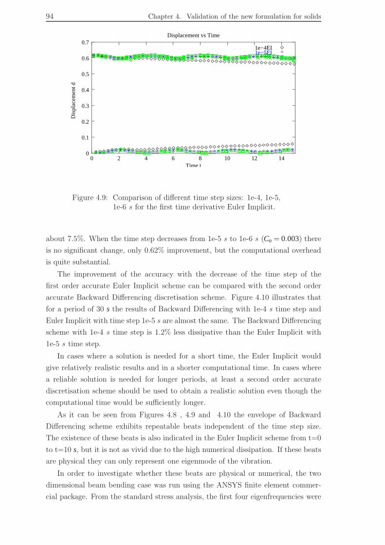
94 Chapter 4. Validation of the new formulation for solids
0
0.1
0.2
0.3
0.4
0.5
0.6
0.7
0 2 4 6 8 10 12 14
Dis
plac
emen
t d
Time t
Displacement vs Time
1e−4EI1e−5EI1e−6EI
Figure 4.9: Comparison of different time step sizes: 1e-4, 1e-5,1e-6 s for the first time derivative Euler Implicit.
about 7.5%. When the time step decreases from 1e-5 s to 1e-6 s (Co = 0.003) there
is no significant change, only 0.62% improvement, but the computational overhead
is quite substantial.
The improvement of the accuracy with the decrease of the time step of the
first order accurate Euler Implicit scheme can be compared with the second order
accurate Backward Differencing discretisation scheme. Figure 4.10 illustrates that
for a period of 30 s the results of Backward Differencing with 1e-4 s time step and
Euler Implicit with time step 1e-5 s are almost the same. The Backward Differencing
scheme with 1e-4 s time step is 1.2% less dissipative than the Euler Implicit with
1e-5 s time step.
In cases where a solution is needed for a short time, the Euler Implicit would
give relatively realistic results and in a shorter computational time. In cases where
a reliable solution is needed for longer periods, at least a second order accurate
discretisation scheme should be used to obtain a realistic solution even though the
computational time would be sufficiently longer.
As it can be seen from Figures 4.8 , 4.9 and 4.10 the envelope of Backward
Differencing scheme exhibits repeatable beats independent of the time step size.
The existence of these beats is also indicated in the Euler Implicit scheme from t=0
to t=10 s, but it is not as vivid due to the high numerical dissipation. If these beats
are physical they can only represent one eigenmode of the vibration.
In order to investigate whether these beats are physical or numerical, the two
dimensional beam bending case was run using the ANSYS finite element commer-
cial package. From the standard stress analysis, the first four eigenfrequencies were

4.4. Results 95
0
0.1
0.2
0.3
0.4
0.5
0.6
0.7
0 5 10 15 20 25 30
Dis
plac
emen
t d
Time t
Comparison of Euler Implicit for 1e−5 time step and Backward Differencing for 1e−4 time step
EI 1e−5BD 1e−4
Figure 4.10: Comparison of Euler Implicit using time step size1e-5 s against Backward differencing using time stepsize of 1e-4 s (envelope of displacement).
n 1 2 3 4
fn 0.677 3.2102 4.2015 5.0791
Table 4.2: Computational calculations for the vibrationeigenfrequencies of vibration using for the twodimensional beam bending case using the ANSYS finiteelement commercial package.

96 Chapter 4. Validation of the new formulation for solids
0
0.1
0.2
0.3
0.4
0.5
0.6
0.7
0 5 10 15 20 25 30
Dis
plac
emen
t d (
m)
Time t (sec)
Mesh resolution comparison 40x10, 60x20BD, 200x50BD
40x1060x20BD
200x50BD
Figure 4.11: Mesh resolution comparison for meshes: 40x10, 60x20and 200x50 cells. Time step size used is 1e-4 andtemporal term discretisation scheme is Backwarddifferencing (envelope of displacement).
obtained (Table 4.2 ). It should be mentioned that the first four eigenmodes are
fundamental and the rest of the frequencies are combination of the first four. The
beats appearing in the envelope of displacement of our discretisation have a fre-
quency of 0.2369 Hz, where the frequency of the first mode found by ANSYS is
0.677 Hz. Thus, it can be concluded that their appearance is of numerical nature.
These errors relate to the mesh quality as it is illustrated in the following section.
4.4.2.3 Mesh quality
In this section, the numerical errors introduced due to mesh quality are examined.
Up to now, the grid was 40x10 cells . In the third dimension there is always one
cell. As this is a two dimensional investigation, displacement and velocity are not
computed in the third direction.
For the other meshes used, the time step is kept to ∆t = 1e−4 s (300,000 time
steps) resulting in a Co = 0.33 and the discretisation scheme for the temporal term
is Backward differencing. The different mesh resolutions applied were 60x20 and
200x50 cells in x and y direction respectively. The results are presented in Fig-
ure 4.11.
All cases run for 30 s. As it can be seen from Figure 4.11 there is very small
dissipation. The displacement envelope beats appears in all three cases but the
number of beats is reduced with the increase of mesh resolution. The frequency of
these beats in the 40x10 cells mesh is 0.1148 Hz, while for 60x20 reduces to 0.1309

4.4. Results 97
0 0.1 0.2 0.3 0.4 0.5 0.6 0.7 0.8 0.9 10
0.1
0.2
0.3
0.4
0.5
0.6
0.7
time (s)
disp
lace
men
t (m
)
Dirichlet using momentumDirichlet using pressure definition
Figure 4.12: Comparison of different boundary conditions forpressure in the fully implicit velocity-pressureformulation.
Hz and for 200x50 drops down to 0.0782 Hz. Thus, for 300,000 time steps for a
200x50 cells mesh, the occurence of the beats is almost dissapearing (only two beats
appear). It should be stressed here that a solution of 300,000 time steps corresponds
to 100 oscillations and the occurence of the beats was no longer examined. Thus, we
need not to conceder further the occurence of the beats. The important finding from
this investigation is that the method proposed in this thesis has minimal dissipation
even if one decides to run the case for very long time.
4.4.3 Boundary conditions
The most difficult part in creating a unified solution method for solving fluid-
structure interaction problems lies in the choice of appropriate boundary conditions.
In the unified method where both velocity and pressure are implicitly solved using
the PISO algorithm for the coupling, a set of boundary conditions is needed for the
velocity and pressure. In Section 2.5 and 3.6 some possible boundary conditions for
the velocity-pressure formulation were derived. There are two issues involved with
the choise of the correct boundary conditions at the free boundary: (a) the equation
that will give a relationship about the behaviour of the variables concerned at the
boundary and (b) the type of the condition i.e. fixed value or fixed gradient.

98 Chapter 4. Validation of the new formulation for solids
In Section 3.4, an extensive literature review is presented on boundary conditions
for incompressible fluids that lead us to the choice of the appropriate boundary
conditions for compressible fluid-structure interaction problems using the unified
solution method. The appropriate boundary conditions for velocity is fixed gradient
and is derived from the force balance equation at the boundary (Equation 3.70) and
for the pressure is fixed value derived from the momentum (Equation 3.76).
As far as the first issue is concerned the derivation of the optimal pressure bound-
ary condition is according to the paper of Gresho and Sani (1987) but for a com-
pressible material. In Figure 4.12 it is demonstrated the accurate solution of the
fully implicit velocity pressure formulation using boundary conditions for pressure
according to Gresho and Sani (1987) in contrast to the suboptimal choice such as
the use of the definition of pressure at the boundary.
4.4.4 Other cases
In this section variations of the beam bending case are presented. These cases were
run in order to get another validation of the results and the behaviour of the code.
The length of the beam was varied and the following two cases were examined: half
and double the initial length. Another case was selected to run was to use the same
beam length but with the applied end force to be half the initial one.
4.4.4.1 Analytical solution
For the beam with half the original length (5mx10m) using the analytical solution,
the end displacement is found to be 0.0995 m and the frequency of the beam os-
cillation is 13.413 Hz. For the beam with double the length (40mx10m) the end
displacement is 5.198 m and the frequency should be 0.8384 Hz. For the beam
where the end shear applied is τ = 5e5Pa, the end displacement is 0.34 m and the
frequency of the beam oscillation is 3.35 Hz.
4.4.4.2 Numerical solution
In all cases the time step used was ∆t = 1e−4 s, the temporal discretisation scheme
applied was Backward differencing and the mesh resolution was kept equivalent
with the beam length i.e. constant ∆x. For the case with half the beam length
(10mx5m) the mesh used was 20x10 cells. The end displacement found was 0.087
m and the frequency was 11.64 Hz (Figure 4.13). The percentage difference for the
frequency between the analytical solution and the numerical solution is 13.29 % and
for the maximum displacement is 12.96 % (Table 4.3). It must be noted that as the
analytical solution is 1D, the shorter the beam is in relation to its height, the less
accurate the solution would be. This can explain the 12.96 % difference with the
numerical solution.

4.4. Results 99
Variable Analytical Predicted % DifferenceBeam size: 10mx5m; end shear: 1e6 Pa
Max Displacement [m] 0.0995 0.0866 12.96Frequency [Hz] 13.41 11.64 13.29
Beam size: 20mx5m; end shear: 1e6 PaMax Displacement [m] 0.68 0.62 8.82Frequency [Hz] 3.35 3.32 0.9
Beam size: 40mx5m; end shear: 1e6 PaMax Displacement [m] 5.2 4.72 9.21Frequency [Hz] 0.84 0.86 2.05Beam size: 20mx5m; end shear: 5e5 PaMax Displacement [m] 0.34 0.313 7.94Frequency [Hz] 3.35 3.29 1.79
Table 4.3: Comparison between analytical and computationalsolution for beams with different size.
0 0.1 0.2 0.3 0.4 0.5 0.6 0.7 0.8 0.9 10
0.01
0.02
0.03
0.04
0.05
0.06
0.07
0.08
0.09
Dis
plac
emen
t (m
)
Time (sec)
Figure 4.13: Beam with size 10mx5m. No of cells used for themesh is 20x10cells , time step size used is 1e-4 andtemporal term discretisation scheme is Backwarddifferencing.

100 Chapter 4. Validation of the new formulation for solids
0 0.5 1 1.5 2 2.5 3 3.5 4 4.5 50
0.5
1
1.5
2
2.5
3
3.5
4
4.5
5
Dis
plac
emen
t (m
)
Time (sec)
Figure 4.14: Beam with size 40mx5m. No of cells used for themesh is 80x10cells , time step size used is 1e-4 s andtemporal term discretisation scheme is Backwarddifferencing.
For the case with double beam length (40mx5m) the mesh used was 80x10 cells
(Figure 4.14). The end displacement was 4.72 m and the frequency was 0.859 Hz .
The percentage difference between the analytical and the numerical solution is 2.05
% and for the displacement 9.21% (Table 4.3).
In the case where the applied end shear was halved τ = 5e5Pa, the time step used
was ∆t = 1e−4 s, the temporal discretisation scheme used was Backward differenc-
ing and the mesh resolution was 40x10 cells, the same as the one in the standard
validation case. Figure 4.15 presents the results. The maximum end displacement is
0.313 m and the frequency of oscillation of the beam is 0.29 Hz. The percentage dif-
ference for the frequency between the analytical solution and the numerical solution
is 1.79 % and for the maximum displacement is 7.94 % (Table 4.3).
4.5 Closure
In Chapter 2 the derivation of the unified solution method for solving fluid-structure
interaction problems was presented. As the method is standard for solving fluids
validation is needed only for solids. In this Chapter, a two dimensional beam bending
case was chosen for the validation, which is more difficult to solve as it comprises,

4.5. Closure 101
0 0.1 0.2 0.3 0.4 0.5 0.6 0.7 0.8 0.9 10
0.05
0.1
0.15
0.2
0.25
0.3
0.35
Time (sec)
Dis
plac
emen
t (m
)
Figure 4.15: Beam with size 20mx5m, with applied end shearτ = 5e5Pa. No of cells used for the mesh is 40x10cells, time step size used is 1e-4 s and temporal termdiscretisation scheme is Backward differencing.

102 Chapter 4. Validation of the new formulation for solids
shear stress as well, rather than normal stress only. The effect of shear is of great
importance in wave propagation in fluid structure interaction problems.
In Chapter 3, several discretisation issues were raised that have been examined
here. The way the terms are discretised in the momentum equation affects the
behaviour of the system. If the discretisation of the accumulated terms is done in
an inconsistent way, different discretisation errors are induced that lead to inaccurate
results. Consistent discretisation removes the erratic behaviour of the net energy.
In Section 3.7, a stability analysis was performed for the displacement based
formulation and compared with the velocity-based formulation. In this Chapter,
we have illustrated this behaviour with a numerical example. A velocity-based
formulation for solids where the trapezoid rule has been used, for the introduction of
the velocity instead of displacement in the stress tensor, results in an accurate system
without the need to use more accurate schemes such as Newark. The displacement
based formulation, which is first order accurate, completely dissipates after 170,000
time steps whereas the velocity formulation after 300,000 time steps has dissipated
by only 14.7%. In both cases, the Euler implicit scheme was used.
The comparison of using backward differencing over Euler implicit for the dis-
cretisation of the temporal term in the velocity-pressure formulation has also been
illustrated. The use of Backward Differencing produces a more accurate behaviour
of the numerical model. The decrease of the time step size by a factor of 10 for first
order time derivative Euler Implicit improves the accuracy and brings the results
close to Backward Differencing.
When the beam bending problem needs to be solved for a short period of time,
the Euler Implicit discretisation method will produce relatively good results in a
short period of calculation time. On the other hand, when there is a need for longer
time solution, at least a second order accurate discretisation method should be used
or the time step size should be decreased significantly. In both cases, the increase
of the accuracy is accompanied by an increase of the computational overhead.
In this Chapter, we have illustrated that the PISO algorithm that to the best
of the author’s knowledge has never been used before for structural analysis can
be used successfully for the pressure-velocity coupling in solids. The difficulty in its
correct implementation in a fully implicit velocity-pressure coupling in solids (as well
as in fluids), when a free boundary is used, lies in the choice of appropriate boundary
conditions. The choice involves two issues: the first issue is the choice of the type
(i.e. Dirichlet or Neumann) and the second is the choice of the correct condition that
describes the behaviour of the variable at the boundary. Here, both issues have been
illustrated. The appropriate boundary conditions for solving a fully implicit fluid-
structure interaction problem with the unified solution method are: for the velocity,
a fixed gradient boundary condition, that is obtained by applying the force balance
relation at the boundary and for the pressure a fixed value boundary expression
4.5. Closure 103
that is derived by solving for the normal component of the pressure gradient in the
momentum equation and calculating the value from the gradient.
In Chapter 2, it was concluded that if the mathematical representation of the
unified solution method proves to be able to solve classic solid mechanics problems,
then the unified method probes to work and can be used for solving FSI problems.
In this Chapter as an answer to that question, it was demonstrated that the method
can indeed solve solid mechanics problems accurately. Thus, it has been proved that
a unified solution method can be considered in solving fluid-structure interaction
problems. The next step for the continuation of this project would be to use this
method to solve a full FSI problem. The way it can be used is explained in Chapter
7 which is related to future work.

104 Chapter 4. Validation of the new formulation for solids

Chapter 5
Wave propagation experiments in
flexible vessels with wall thickness
variation and geometric tapering
5.1 Introduction
The study of wave propagation in fluid-filled tubes is often motivated by the need to
understand arterial blood flow. Even though the general principles gathering wave
propagation in flexible vessels are known (McDonald, 1968; Pedley, 1980; Fung,
1997), there is lack in the literature (Section 1.4) of well defined experiments tak-
ing into consideration the wall thickness variation and the geometric tapering that
characterises the human vessels i.e. the aorta. In vitro laboratory experiments in
mechanically and constitutively well-defined systems are needed for the validation
of numerical and analytical models.
To bridge this gap, a set of tubes was designed and manufactured to assess the
role of geometric tapering and wall thickness variation in flexible vessels. The tubes
were manufactured according to aortic specifications. They were designed such that
the wave speed of the travelling wave would be equivalent to that of the aorta. The
experiments were performed for small deformations.
5.2 The Tube Models Methodology
In Section 1.4, it was concluded that there is lack in the literature of well defined
experiments assessing the non-linearities of flexible vessels i.e. wall thickness varia-
tion and geometric tapering. In order to obtain a complete set of experimental data
assessing these variations, a set of flexible tubes was manufactured.
105

106Chapter 5. Wave propagation experiments in flexible vessels with wall thickness
variation and geometric tapering
5.2.1 The vessels design and specifications
The tubes were designed to be model analogues of the human aorta. One of the most
referenced sources of arterial dimensions is the one from Westerhof et al. (1969). In
Table 5.1, the data mentioned in his work are presented. In this work, they are used
as a guidance for the design of the tubes.
Variable Aorta ThoracalisTop internal radius [mm] 20
Bottom internal radius[mm] 11Length [mm] 315
Slope -0.014ϒ∗h/D [MPa] 0.02-0.04
ϒ : Youngs modulus, h: wall thickness, D: internal diameter
Table 5.1: Aorta anatomical data (Westerhof et al., 1969).
To be able to assess the effects of morphological variations in wave propagation
velocity c, six tubes were manufactured: three straight ones and three tapered ones.
The geometrical parameters of these tubes are summarised in Table A.3. It should
be mentioned that the tube of Type E has the same ϒ ∗h/D and wave speed c as
the aorta according to Westerhof et al. (1969) (See Table 5.1).
To separate effects due to geometric tapering, two pairs of tubes were manu-
factured such that they would have the same wave speed throughout according to
linear wave propagation theory (Lighthill, 1975).
The first pair consists of a straight tube with constant wall thickness (Type
A) and a tapered tube with variable wall thickness (Type F). The variable wall
thickness of the tapered tube was chosen such that according to linear theory the
wave speed throughout its length is the same as for the straight tube with constant
wall thickness. In this way the variable wall thickness of the tapered tube according
to the linear theory will counterbalance the effect of geometric tapering.
The second pair consists of a geometrically tapered tube with constant wall
thickness (Type E) and a straight tube with variable wall thickness (Type C). The
variable wall thickness of the tube was designed such that according to linear theory
the wave speed variation along the length of this straight tube is the same as the
for tapered one with constant wall thickness.
The wall thickness variation for tubes C and F can be seen in Figure 5.1.
For reference, a homogeneneous thick walled straight tube (type B) and a ta-
pered, homogeneously thin-walled tube are made as well.

5.2. The Tube Models Methodology 107
Type D[mm] h±0.002[mm] L[mm] z ϒ∗h/D[MPa] c[m/s]
A 25 0.1 446 0 0.04 6.3
B 25 0.05 446 0 0.02 4.5
C 25 0.05-0.1 446 0 0.02-0.04 4.5-6.3
D 25-12.5 0.1 446 -0.014 0.04-0.08 6.3-8.9
E 25-12.5 0.05 446 -0.014 0.02-0.04 4.5-6.3
F 25-12.5 0.1-0.05 446 -0.014 0.04 6.3
ϒ: Young’s modulus, h: wall thickness, D: diameter
Table 5.3: Geometrical parameters of tubes manufactured.

108Chapter 5. Wave propagation experiments in flexible vessels with wall thickness
variation and geometric tapering
0 10 20 30 405
6
7
8
9
10x 10
−3
Tube length [cm]
Thi
ckne
ss o
f tub
e F
[cm
]
0 10 20 30 401
1.5
2
2.5
3
Tube length [cm]
Inte
rnal
dia
met
er o
f tub
e F
[cm
]
0 10 20 30 405
6
7
8
9
10x 10
−3
Tube length [cm]
Thi
ckne
ss o
f tub
e C
[cm
]
0 10 20 30 401.5
2
2.5
3
3.5
Tube length [cm]
Inte
rnal
dia
met
er o
f tub
e C
[cm
]
Figure 5.1: Wall thickness variation for tubes C and F.

5.3. Material Properties of the Tubes 109
5.2.2 Manufacturing Method
The tubes were manufactured by the method of spin coating. The tube takes the
shape of a steel rod that can rotate along its length axis through a servomotor (x-
servomotor). For the straight tubes, this rod is straight, with 25mm diameter and a
length of 500mm. For the tapered tubes a rod with maximum diameter 25 mm and
a minimum diameter of 12.5 mm was used. The length of the taper is 440mm. The
liquid used in the spin coating process, polyurethane (PU, Besmopan 588, Bayer,
Germany) dissolved in tetrahydrofurane (THF, BASF, Germany) is delivered at a
constant flow rate through a nozzle, by a perfusion pump (Harvard medical sytems,
USA). The nozzle is attached to a trolley that can translate along the length of
the rod through by a rotating ball screw rod connected to a second servomotor
(y-servomotor).
The two servomotors are operated simultaneously by a computer-driven servo-
controller. With a given concentration of the PU-solution, flow rate and a required
geometry, the spin-coating device is programmed to generate the proper wall thick-
ness. After evaporation of the solvent, the remaining tube is removed from the rod
and is ready for use.
The process generates tubes with prescribed wall thicknesses (either constant or
variable) with an accuracy of 2 µm.
A detailed description of the manufacturing process is given in Appendix A.
5.3 Material Properties of the Tubes
The physical properties of PU are given in Table 5.4. The solution used had con-
centrations varying from α = 17−22.73%of PU in THF solvent.
Physical properties Polyurothane (PU)
Density(kg/m3) 880Ultimate tensile strength(MPa) 30
Elongation at break (%) 500Tear propagation resistance (kN/m) 55
Table 5.4: Physical properties of polyurethane.
A little solvent remains in the tube. This solvent remnant causes the tube to
have viscoelastic properties. To measure these properties, relaxation tests were
performed. Tensile force at constant strain over time was determined in a uniaxial
tensile testing machine (Zwick Z010, Germany). The specimens measured had a
wall thickness that was double the average of wall thickness of all the tubes, thus

110Chapter 5. Wave propagation experiments in flexible vessels with wall thickness
variation and geometric tapering
10−2
10−1
100
101
102
103
10−3
10−2
10−1
100
101
time [s]
Ten
sile
For
ce [N
]
Figure 5.2: Typical relaxation test curve for Polyurethanespecimen (3% elongation).
5.3. Material Properties of the Tubes 111
it was 0.14 mm. The width of the specimens was 37.3 mm. The specimens were
strained 1%, 3% and 10% to check possible non-linear mechanical behaviour. For
each strain the experiment was repeated six times each on a new specimen.
In Figure 5.2 a typical relaxation test curve is shown. The graph shows two
parts: the behaviour of the specimen under loading until it reaches the strain target
and the specimen relaxed under constant strain.
In linearly viscoelastic materials, it is straightforward to develop a relationship
for the relaxation response ϒ(t). The stress and relaxation modulus relationship is
given by the following Boltzmann integral, where τ is the time variable of integration:
σ(t) =
Z t
0ϒ(t − τ)
dε(τ)dτ
dτ (5.1)
In the integral form, the time scale is considered just prior to time zero, so that
step function load histories beginning at zero may be accomplished.
As the Figure 5.2 shows, the stress in the material decays with time. A power
law model is suitable to describe this material phenomenologically:
ϒ(t) = ct−n (5.2)
The integral of Equation 5.1 using the derivative theorem and the convolution
theorem, with s the transformation variable, can be transformed to:
σ(s) = sϒ(s)ε(s) (5.3)
It should be noted that the relaxation modulus is complex in the frequency
domain. Taking the Laplace transform of ϒ(t) and recognising Γ, as the gamma
function, defined as follows:
Γ(x) =
Z ∞
0tx−1e−tdt (5.4)
the complex Young’s modulus then is expressed as:
ϒ(s) = cΓ(1−n)sn (5.5)
The complex viscoelastic modulus can be written as a function of the angular
frequency as follows:
ϒ(ω) = cΓ(1−n)ωnei nπ2 (5.6)
The values of c and n can be obtained from data fitting of the relaxation test data
using the power law (Equation 5.2). This is done by using a standard Nelder-Mead
minimisation scheme, as implemented in Matlab 6.5 (The MathWorks, Natick MA,
USA)

112Chapter 5. Wave propagation experiments in flexible vessels with wall thickness
variation and geometric tapering
The following values of c and n are obtained: 2.3 · 106 [Pas−n] and 0.065[−]
respectively. The real part of the complex modulus, the storage modulus relates to
the elastic behaviour of the material and defines the stiffness of the material. The
imaginary part is the loss modulus and relates to the materials viscous behaviour
and defines the energy dissipative ability of the material. This values result in a loss
modulus less than 10% of the value of the storage modulus. Therefore for modelling
purposes the tubes can be modelled as purely elastic. The Young’s modulus of
Polyurethane can be obtained by Rutten (1998):
ϒ =1
N+1
N
∑i=0
Re[ϒi(s)] (5.7)
where N is the harmonic number corresponding to the bandwidth of the excita-
tion signal. In our case it is 40. The Youngs modulus was calculated to be 1.72MPa.
5.4 Measurement Methods
5.4.1 Experimental set-up
A schematic diagram of the experimental set-up used to carry out wave propagation
experiments in flexible vessels is shown in Figure 5.3. The apparatus consists of a
tube marked as (F) in the schematic diagram, placed in horizontal position inside an
open container (E) filled with water. The water depth above the tube prescribes the
pressure outside the vessel. The tube is pre-strained axially to 3% in order keep it in
a straight after it is filled with water. The tube is fixed on both sides and can expand
freely in the radial direction along its length. On one side, the tube has a closed end
and, on the other side, it is connected to a three way solenoid valve (B) operated by
a PC. The valve is connected at one side to a closed tank (C) and at the other side
to a two way manually operated valve (A). The closed tank (C) is maintained at a
constant pressurise of about 1 bar. The two way valve (A) is connected to an open
tank (D). The system is filled with water. When the solenoid valve is not engaged the
water column level inside the open tank (D) prescribes the pressure inside the tube.
A block shaped pulse can be initiated through the PC. The duration of the opening
of the valve which initiates the pulse was set to be 0.05 s. It is essential that the
duration of the opening of the valve is as short as possible because the wavelength
of the waves should be as short as possible, to enable distinction between forward
and backward travelling waves. Furthermore, as little as possible liquid should be
injected into the tube, to keep the stationary pressure rise during the experiment as
low as possible. The flow rate meter (Q) and the ultrasound probe (W) were held
stationary by retort-stand and clip. The ultrasound scanner was positioned so that
the ultrasound beam is sent perpendicular to the surface of the tube. Each one of

5.4. Measurement Methods 113
the pressure catheters (P1,P2) was introduced via a junction beyond the closed end
of the bath in which the tube is fixed.
A: two way manual operated valve, B: three way solenoid valve operated by a PC, C:closed tank pressurised at about 1 bar, D: open tank, E: open container filled withwater, F: tube, P1 and P2: pressure catheters, Q: volumetric flow rate meter, W:wall motion ultrasound scanner.
Figure 5.3: Experimental set-up for wave propagation experiments(TU/e).
5.4.2 Instrumentation
Pressure and pressure gradient
Two pressure-wire sensors (Radi Medical Systems 12000XT ) were used to mea-
sure the pressure simultaneously at two points along the tube, 17 mm apart. The
pressure wires were of 0.36 mm diameter, typically used for clinical measurements.
Each pressure wire was connected to a Radi Medical Systems interface box. The
interfaces introduce a time-delay in the signal due to the internal processing. This
time delay was determined using a real-time analogue pressure measurement with
Beckton Dickinson pressure sensor (PZ10E) in combination with a Peekel CA253
bridge amplifier. The time-shift between the pressures as simultaneously measured
by the Radi pressure-wire and the BD PZ10E was determined by cross-correlation

114Chapter 5. Wave propagation experiments in flexible vessels with wall thickness
variation and geometric tapering
of the two signals and turned out to be 10 ms. The time-shift was accounted for in
the subsequent data processing.
Flow rate
The fluid flow rate was measured using a perivascular flow rate sensor (type MC28AX,
Transonic, the Netherlands), with an inside diameter of 28 mm and a bandwidth
of 160 Hz. The sensor is suitable for measurements of vessels with 22-28 mmouter
diameter allowing maximum distension of the tubes without them touching at the
surface of the probe. The probe was connected to its interface box and the signal
was passed to a PC.
Wall motion
The wall motion was measured using an ultrasound wall track system (Brands
et al., 1999). This single-beam ultrasound system acquires the RF-echo signal at
a pulse repetition Frequency of 1000 Hz and is stored in the computer memory
during acquisition. After the measurement (typical duration 4 seconds) the RF-
matrix is stored to the hard disk for further processing. The wall displacement data
are extracted from the RF-matrix by cross-correlation using the filtering technique
described in Brands et al. (1999). This yields a spatial resolution of 250 µm and a
temporal resolution of 1/200 s.
5.4.3 Protocol
For each one of the six tubes four instantaneous time variables were measured:
Pressure, pressure gradient, flow rate and wall distension. The measurements were
taken at 10 positions (z) along the tube length, each 50 mm apart. The positioning
of the flow probe and the ultrasound scanner was accommodated by a ruler. The
two pressure wires were placed at the two edges of the flow probes width, in order
to have flow rate and pressure gradient measured at the same location.The distance
between the two wires was 17 mm. For every measurement this distance was kept
constant by accurately positioning the two sensors using a stereo microscope. From
the two pressure measurements, the pressure gradient was obtained.
Before each measurement, the pressure wires were calibrated to zero against
the hydrostatic pressure imposed to the tube by the open air tank. During the
measurements, the two way valve (A) connected to the open air tank was kept
closed in order to preserve the volume of the water induced in the tube by the
opening of the solenoid valve. The signals for pressure, pressure gradient and flow
rate for each measurement 1000 samples/s were taken using LabView software with
National Instruments hardware. To avoid any loss of signal, all measurements were
5.5. Results 115
taken with no extra filtering. For the wall movement measurements, the RF-signal
received by the echo scanner was obtained and stored for 2 s.
At each position, the measurements were repeated 16 times in order to obtain the
mean for each variable. The standard deviation at 16 measurements is at about the
noise level of the pressure sensors, so more measurement would not have increased
the accuracy.
5.4.4 Data processing
Pressure and pressure gradient
The data processing of the digitised pressure measurements starts with phase shift
correction between the two signals introduced by the different Radi Medical System
pressure wire interfaces. The signals were fast-Fourier transformed and, by examin-
ing the signal spectrum, undesired noise peaks were identified and filtered without
inducing any phase shift.
Wall distension
Once the RF signal (reflected and scattered) has been recorded and transferred to
the computer, the digitised RF signal as a function of depth is displayed on the
computer screen. The tube lumen and wall interface can be identified by the shape
of the signal. Indicator markers have to be manually placed on the reflections of
the anterior and posterior tube walls to indicate the initial search area for the wall-
detection algorithm. The algorithm then tracks the position of the walls over time.
This renders the wall positions and therefore the lumen diameter as a function of
time.
5.5 Results
5.5.1 Static pressure - initial diameter relation
In order to ensure that the the tubes undergo small deformations during the ex-
periments, the pressure-initial diameter relatio was measured for the thin straight
tube (Tube B) by applying different pressures inside the tube. The different levels
of pressure were defined by the different water levels in the open tank. As can be
seen from Figure 5.4, the tube’s behaviour is linear throughout the pressure range
considered. The corresponding circumferential strains are less than than 3% and
may therefore be considered small. The initial pressure inside the tube was set to
2.94 kPa.

116Chapter 5. Wave propagation experiments in flexible vessels with wall thickness
variation and geometric tapering
1 1.5 2 2.5 3 3.5 4 4.52.38
2.4
2.42
2.44
2.46
2.48
2.5
2.52
2.54
2.56x 10
4
Static pressure [kPa]
Initi
al D
iam
eter
[um
]
Figure 5.4: Static pressure-initial diameter relation of the straighttube (Type B).

5.5. Results 117
5.5.2 Standard deviation of measurements
For each tube, the four instantaneous time variables measured at 10 locations along
the tube length are shown in Sections 5.5.3 and 5.5.4. For each tube at every
location, the mean of 16 measurements and the standard deviation from the mean
were calculated to assess the reliability and repeatability of the results for each one
of the measured variables. The standard deviation is calculated from:
σ =
√∑n
i=1(xi −x)2
n−1(5.8)
A typical result can be seen in Figure 5.5.
0 0.2 0.4 0.6 0.8 1−4
−2
0
2
4
6
8
Flo
w r
ate
Q [l
/min
]
Time t [s]
meanmean+stdmean−std
0 0.2 0.4 0.6 0.8 1−5
0
5
10
15
Pre
ssur
e P
[mm
Hg]
Time t [s]
Tube type B axial location along its length: 100 [mm]
meanmean+stdmean−std
0 0.2 0.4 0.6 0.8 1−100
0
100
200
300
400
500
Wal
l dis
tent
ion
[um
]
Time t [s]
meanmean+stdmean−std
0 0.2 0.4 0.6 0.8 1−3
−2
−1
0
1
2
3
Pre
ssur
e gr
adie
nt
Time t [s]
meanmean+stdmean−std
Figure 5.5: A typical result at a location showing the mean of 16measurements and the standard deviation from themean.
5.5.3 Fluid motion
The three measurements related to the fluid motion were: the pressure, the flow
rate and the pressure gradient. It should be mentioned that only the mean value of
the 16 measurements at each location is presented. In the following sub-sections in

118Chapter 5. Wave propagation experiments in flexible vessels with wall thickness
variation and geometric tapering
order to be able to draw comparative conclusions the results presented have been
scaled in amplitude so as the initial pulse has the same amplitude in all tubes. The
time is also scaled using the peak-to-peak value of the first reflection.
Pressure
The normalised mean pressure measurements for various axial positions along the
length of the tube is plotted against scaled time. The three straight tubes can be
seen in Figure 5.6 and the three tapered ones in Figure 5.7. In Figures 5.8, the
pressure propagation for tubes A and F is compared and, in 5.9, the propagation
for tubes C and E is compared.
0 0.05 0.1 0.15 0.2 0.25 0.3 0.35 0.4 0.45 0.5Scaled time
Axi
al p
ositi
on
Pressure propagation
CAB
Figure 5.6: Normalised pressure measurements every 50 mm alongthe length of the tube against scaled time for straighttubes: types A,B,C (A: straight tube with constantwall thickness of 0.1 mm; B: straight tube withconstant wall thickness of 0.05 mm; C: straight tubewith variable wall thickness of 0.05-0.1 mm).
Figure 5.6 shows that the straight tube with variable wall thickness has slightly
higher amplitude than the other straight ones. The shape of the pulse in all three
of them is similar.

5.5. Results 119
0 0.05 0.1 0.15 0.2 0.25 0.3 0.35 0.4 0.45 0.5Scaled time
Axi
al p
ositi
on
Pressure propagation
FDE
Figure 5.7: Normalised pressure measurements every 50 mm alongthe length of the tube against time for tapered tubes:types D,E,F (D: tapered tube with constant wallthickness of 0.1 mm; E: tapered tube with constantwall thickness of 0.05 mm; F:tapered tube withvariable wall thickness of 0.1-0.05 mm).
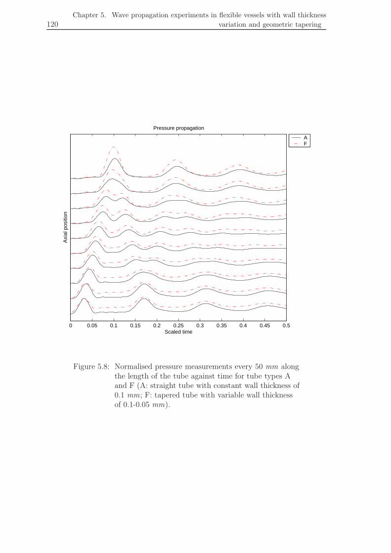
120Chapter 5. Wave propagation experiments in flexible vessels with wall thickness
variation and geometric tapering
0 0.05 0.1 0.15 0.2 0.25 0.3 0.35 0.4 0.45 0.5Scaled time
Axi
al p
ositi
on
Pressure propagation
AF
Figure 5.8: Normalised pressure measurements every 50 mm alongthe length of the tube against time for tube types Aand F (A: straight tube with constant wall thickness of0.1 mm; F: tapered tube with variable wall thicknessof 0.1-0.05 mm).
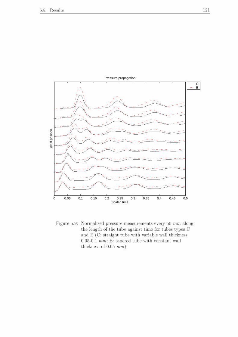
5.5. Results 121
0 0.05 0.1 0.15 0.2 0.25 0.3 0.35 0.4 0.45 0.5Scaled time
Axi
al p
ositi
on
Pressure propagation
CE
Figure 5.9: Normalised pressure measurements every 50 mm alongthe length of the tube against time for tubes types Cand E (C: straight tube with variable wall thickness0.05-0.1 mm; E: tapered tube with constant wallthickness of 0.05 mm).

122Chapter 5. Wave propagation experiments in flexible vessels with wall thickness
variation and geometric tapering
From Figure 5.7 it can be seen that the pressure wave of the two tubes with
constant wall thickness (D and E) matches closely in amplitude and shape. The
tube with the variable wall thickness (F) has slightly lower amplitude at the distal
end, than the other two. The shape of the pulse between the first and the second
reflection at the distal end is slightly less steep.
In Figure 5.8 Tube F has been manufactured with wall thickness variation, to
have the same wave velocity according to the linear theory along its length as the
straight with constant wall thickness (Tube A). Thus, the wall thickness variation
was expected to counterbalance for the tubes tapering. However, it is evident in
Figure 5.8 that the tapering increases the pressure amplitude towards the distal end
while the wave velocity also increases. At the distal end between the two peak-to-
peak values it can be seen that the tapering affects the shape of the pulse as it rises
faster, where as in the straight one it remains flat until the next reflection.
In Figure 5.9, the straight Tube C was manufactured with wall thickness varia-
tion, to have the same wave velocity according to the linear theory as the tapered
one with constant wall thickness (Type E). Thus, the wall thickness variation is
expected to give a similar effect in the propagation as the tapering. However, this
is not the case. It can be seen from the graph that the wall thickness variation
cannot accommodate the non-linear effects introduced by the geometric tapering.
The pressure amplitude is significantly higher due to the tapering and the shape of
the pulse is again different at the distal end and the rise of the pulse between the
first and the second peak.
Thus, the results suggest that for the pressure wave the tapering effects are strong
and cannot be counterbalanced with the wall thickness variation. The tapering leads
to higher pressure amplitude and the shape of the pressure pulse is different due to
the tapering.
Flow rate
The normalised mean flow rate measurements for the various axial positions along
the length of the tube is plotted against scaled time. The results from the three
straight tubes can be seen in Figure 5.10 and from the three tapered ones in Figure
5.11. In Figures 5.12, the measurements from tubes A and F and, in Figure 5.13,
from tubes C and E are presented.
From Figure 5.10, it can be seen that the straight tubes have about the same
wave form shape and the same amplitude. The tube with the wall thickness variation
has slightly lower amplitude. From Figure 5.11, it can be seen that the three tapered
tubes have the same wave form shape. The amplitude of the flow rate for the tube
with the variable wall thickness (Tube F), is slightly higher than the other two.
In Figure 5.12, where the results from the tube pair A and F are compared, it is
seen that the amplitude of the flow rate wave reduces. This is expected as it has

5.5. Results 123
0 0.05 0.1 0.15 0.2 0.25 0.3 0.35 0.4 0.45 0.5Scaled time
Axi
al p
ositi
on
Flow propagation
CAB
Figure 5.10: Normalised flow rate measurements every 50 mmalong the length of the tube against scaled time forstraight tubes: types A, B, C (A: straight tube withconstant wall thickness of 0.1 mm; B: straight tubewith constant wall thickness of 0.05 mm; C: straighttube with variable wall thickness of 0.05-0.1 mm).

124Chapter 5. Wave propagation experiments in flexible vessels with wall thickness
variation and geometric tapering
0 0.05 0.1 0.15 0.2 0.25 0.3 0.35 0.4 0.45 0.5Scaled time
Axi
al p
ositi
on
Flow propagation
FDE
Figure 5.11: Normalised flow rate measurements every 50 mmalong the length of the tube against scaled time forstraight tubes: types D, E, F (D: tapered tube withconstant wall thickness of 0.1 mm; E: tapered tubewith constant wall thickness of 0.05 mm; F: taperedtube with variable wall thickness of 0.1-0.05 mm).

5.5. Results 125
0 0.05 0.1 0.15 0.2 0.25 0.3 0.35 0.4 0.45 0.5Scaled time
Axi
al p
ositi
on
Flow propagation
AF
Figure 5.12: Normalised flow rate measurements every 50 mmalong the length of the tube against time for tubestypes A and F (A: straight tube with constant wallthickness of 0.1 mm; F: tapered tube with variablewall thickness of 0.1-0.05 mm).

126Chapter 5. Wave propagation experiments in flexible vessels with wall thickness
variation and geometric tapering
0 0.05 0.1 0.15 0.2 0.25 0.3 0.35 0.4 0.45 0.5Scaled time
Axi
al p
ositi
on
Flow propagation
CE
Figure 5.13: Normalised flow rate measurements every 50 mmalong the length of the tube against time for tubestypes C and E (C: straight tube with variable wallthickness 0.05-0.1 mm; E: tapered tube with constantwall thickness of 0.05 mm).

5.5. Results 127
been previously observed that the equivalent pressure signal had increased due to
the tapering. The same observations apply for the tube pair C and E as shown in
Figure 5.13.
These observations indicate that the geometric tapering strongly decreases the
amplitude of the wave signal. The wall thickness variation on the other hand does
not play any significant role apart from slightly reducing the amplitude compared
to the constant thickness tubes.
Pressure Gradient
The normalised mean pressure gradient measurements for the various axial positions
along the length of the tube is plotted against scaled time. The result from the three
straight tubes can be seen in Figure 5.14 and the three tapered ones in Figure 5.15.
In Figure 5.16 the results from tubes A and F are shown and in Figure 5.17 the
results from tubes C and E are shown.
In Figure 5.14 the results from the straight tubes are compared. The shape of
the pressure gradient at the entrance of the tube for the tube Type C (with wall
thickness variation), is the same as the one Type B. Throughout the propagation
towards the distal end their behaviour is quite close. In Figure 5.15, where all
the tapered tubes are compared, it can be seen that the tubes with the same wall
thickness at the entrance of the wave i.e. Type D and F have the same shape for the
pressure gradient. From the graphs it is suggested that the shape of the pressure
gradient at the entrance of of the wave depends on the wall thickness of the tube
at the entrance. From Figures 5.16 and 5.17 it can be observed that the geometric
tapering has an affect on the amplitude of the pressure gradient, in particular it
increases towards the distal end. If the results of the two pairs of tubes (A and F
versus C and E) are compared together, it is clear that for each pair the shape is
comparable but the two pairs themselves have different shape. This leads to the
conclusion that the shape of the pulse at the entrance depends on the thickness of
the wall at the entrance of the tube.
Thus, the wall thickness variation plays a role in the shape of the pressure gradi-
ent. The geometric tapering affects the amplitude of the signal and forces it to rise
significantly compared to the straight one.
5.5.4 Wall motion
The normalised mean wall distension measurements for the various axial positions
along the length of the tube is plotted against scaled time.
The measurements for the three straight tubes are shown in Figure 5.18 and
the three tapered ones in Figure 5.19. In Figures 5.20 and 5.21, the two pairs are
presented.

128Chapter 5. Wave propagation experiments in flexible vessels with wall thickness
variation and geometric tapering
0 0.05 0.1 0.15 0.2 0.25 0.3 0.35 0.4 0.45 0.5Scaled time
Axi
al p
ositi
on
Pressure gradient propagation
CAB
Figure 5.14: Normalised pressure gradient measurements every 50mm along the length of the tube against time fortubes types A, B, C (A: straight tube with constantwall thickness of 0.1 mm; B: straight tube withconstant wall thickness of 0.05 mm; C: straight tubewith variable wall thickness of 0.05-0.1 mm).

5.5. Results 129
0 0.05 0.1 0.15 0.2 0.25 0.3 0.35 0.4 0.45 0.5Scaled time
Axi
al p
ositi
on
Pressure gradient propagation
FDE
Figure 5.15: Normalised pressure gradient measurements every 50mm along the length of the tube against time fortubes types D, E, F (D: tapered tube with constantwall thickness of 0.1 mm; E: tapered tube withconstant wall thickness of 0.05 mm; F: tapered tubewith variable wall thickness of 0.1-0.05 mm).

130Chapter 5. Wave propagation experiments in flexible vessels with wall thickness
variation and geometric tapering
0 0.05 0.1 0.15 0.2 0.25 0.3 0.35 0.4 0.45 0.5Scaled time
Axi
al p
ositi
on
Pressure gradient propagation
AF
Figure 5.16: Normalised pressure gradient measurements every 50mm along the length of the tube against time fortubes types A and F (A: straight tube with constantwall thickness of 0.1 mm; F: tapered tube withvariable wall thickness of 0.1-0.05 mm).
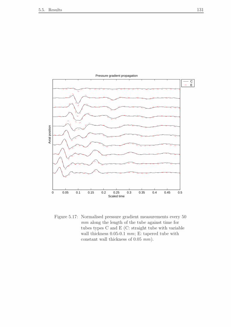
5.5. Results 131
0 0.05 0.1 0.15 0.2 0.25 0.3 0.35 0.4 0.45 0.5Scaled time
Axi
al p
ositi
on
Pressure gradient propagation
CE
Figure 5.17: Normalised pressure gradient measurements every 50mm along the length of the tube against time fortubes types C and E (C: straight tube with variablewall thickness 0.05-0.1 mm; E: tapered tube withconstant wall thickness of 0.05 mm).

132Chapter 5. Wave propagation experiments in flexible vessels with wall thickness
variation and geometric tapering
0 0.05 0.1 0.15 0.2 0.25 0.3 0.35 0.4 0.45 0.5Scaled time
Axi
al p
ositi
on
Wall distension propagation
CAB
Figure 5.18: Normalised wall motion measurements every 50 mmalong the length of the tube against time for tubestypes A, B, C (A: straight tube with constant wallthickness of 0.1 mm; B: straight tube with constantwall thickness of 0.05 mm; C: straight tube withvariable wall thickness of 0.05-0.1 mm).

5.5. Results 133
0 0.05 0.1 0.15 0.2 0.25 0.3 0.35 0.4 0.45 0.5Scaled time
Axi
al p
ositi
on
Wall distension propagation
FDE
Figure 5.19: Normalised wall motion measurements every 50 mmalong the length of the tube against time for tubestypes D, E, F (D: tapered tube with constant wallthickness of 0.1 mm; E: tapered tube with constantwall thickness of 0.05 mm; F: tapered tube withvariable wall thickness of 0.1-0.05 mm).

134Chapter 5. Wave propagation experiments in flexible vessels with wall thickness
variation and geometric tapering
0 0.05 0.1 0.15 0.2 0.25 0.3 0.35 0.4 0.45 0.5Scaled time
Axi
al p
ositi
on
Wall distension propagation
AF
Figure 5.20: Normalised wall motion measurements every 50 mmalong the length of the tube against time for tubestypes A and F (A: straight tube with constant wallthickness of 0.1 mm; F: tapered tube with variablewall thickness of 0.1-0.05 mm).

5.5. Results 135
0 0.05 0.1 0.15 0.2 0.25 0.3 0.35 0.4 0.45 0.5Scaled time
Axi
al p
ositi
on
Wall distension propagation
CE
Figure 5.21: Normalised wall motion measurements every 50 mmalong the length of the tube against time for tubestypes C and E (C: straight tube with variable wallthickness 0.05-0.1 mm; E: tapered tube with constantwall thickness of 0.05 mm).

136Chapter 5. Wave propagation experiments in flexible vessels with wall thickness
variation and geometric tapering
From Figure 5.18, it can be seen that the wall thickness variation significantly
reduces the amplitude of the wall distension as the tube gets thicker towards its distal
end. Comparing tube Type F with D and E, in Figure 5.19, it is indicated that the
wall thickness variation affects again the amplitude of the wave. The more the tube
becomes thinner towards the distal end the more the wall distension increases. In
Figures 5.20 and 5.21, the two pairs are compared. It is evident that the geometric
tapering decreases the amplitude of the wall motion towards the distal end. Thus,
the wall thickness variation can reduce the amplitude of the wave. This effect is
expected from linear theory. The geometric tapering reduces the amplitude of the
wall distension signal, which is expected from linear theory (Laplace’s law).
5.6 Closure
From the comparison of the experimental data, it is concluded that, for the pressure
wave, the tapering effects are strong and cannot be counterbalanced with the wall
thickness variation. The tapering leads to higher pressure amplitude and the shape
of the pressure pulse is different due to the tapering. This is in agreement with the
findings of Belardinelli and Cavalcanti (1992), who studied the effect of tapering in
wave propagation using a two-dimensional non-linear theory. The geometric tapering
strongly decreases the amplitude of the flow wave which is expected to have the
opposite effect to the pressure. The wall thickness variation does not play any
significant role in the flow rate apart from slightly reducing the amplitude of the
signal. The shape of the pressure gradient at the entrance of the wave depends on
the wall thickness of the tube at the entrance. The geometric tapering affects the
amplitude of the gradient and makes it rise compared to the straight one. The wall
thickness variation can reduce the amplitude of the signal, but this effect is expected
from the linear theory. The geometric tapering reduces the amplitude of the wall
distension signal, which is expected from linear theory.
The fact the the shape of the pressure pulse is changed by the geometric tapering
effect is a very important observation in cardiovascular research as pressure is often
used as a tool for diagnosis. Thus, for the correct evaluation of the pressure in
the aorta the geometric tapering has to be taken into account in the computational
models. This directly implies that non-linear theory needs to be incorporated in
modelling the aorta. The wall thickness variation on the other hand, does not have
any significant effect apparent from slightly increasing the pressure amplitude and
this can be corrected by using the correct wave velocity using linear methods.

Chapter 6
Comparison of experimental
results with linear wave
propagation methods
6.1 Introduction
In Chapter 5, a complete experimental data set was presented on the role of geo-
metric tapering and wall thickness variation in flexible vessels. Some of the tubes
measured were designed in pairs according to linear theory in order to have the same
wave propagation velocity. It was concluded that the linear theory cannot predict
the amplitude and the shape of the pulse that alters due the constant reflections
from the tapered wall. In this chapter, the quality of the measurements only for the
straight tubes is tested by comparing them with the linear wave theory. Two cases
are examined; one with purely elastic wall and the second with viscoelastic wall. It
is expected that there will be good agreement between the measurements and the
predictions using the linear theory.
In the first part of this chapter, the main points of the linear theory are outlined
and, in the second part, comparisons between experiments and predictions using
purely elastic or viscoelastic material are presented. The chapter concludes with a
discussion of the main findings from the comparisons.
6.2 Linear Theory of Wave Propagation in Flexi-
ble Vessels
The theoretical investigation of the propagation of pressure disturbances in disten-
sible tubes containing an inviscid fluid has been performed by many researchers
(Section 1.4). The basic theory for a circular uniform flexible tube filled with a
viscous fluid is often referred to as “Womersley theory” (Womersley, 1957). This
137

138Chapter 6. Comparison of experimental results with linear wave propagation
methods
r
z
ξ = ξ(z, t)
ζ = ζ(z, t)
θ
h
r
P
P’
Figure 6.1: Tube motion variables. Point P(z, r) on the surface ofthe wall at rest displaces to position P’(z+ζ, r +ξ) .
theory can be found in many text books such as McDonald (1968); Pedley (1980);
Lighthill (1978) and is outlined here.
6.2.1 Basic theory
The momentum equation (Equation 6.1) and continuity equation (Equation 6.2) for
incompressible Newtonian fluids in a uniform elastic tube of finite length under the
assumption that the flow is axi-symmetric, can be solved in the frequency domain
after linearisation. The equations are:
ρ∂U∂t
+ρ∇ •(UU) = ∇ •(η∇U)−∇p (6.1)
∇ •U = 0 (6.2)
The wave length λ (λ = 2π cω) of the disturbance of interest is assumed to be long
compared to the diameter 2ro of the tube ( λ2r0
≫ 1 ). It is convenient to make the
the Navier-Stokes equations non-dimensional. Therefore U′z and U
′r are considered
as typical velocities in the axial (z) and radial (r) directions respectively. The ratio
between the two velocities is defined by κ = U′r
U ′z, and in the following treatment κ is
considered to be small and L/2r0 ≫ 1. Provided that the Mach numbers
∣∣∣∣U
′r
c
∣∣∣∣≪ 1
and
∣∣∣∣U
′z
c
∣∣∣∣≪ 1, the convective terms plus all velocity derivatives in the z direction in
Equation 6.1 can be neglected (Barnard et al., 1966; Reuderink et al., 1993).
The non-dimensional form of the Navier-Stokes equations in cylindrical coordi-
nates under axisymmetric conditions (θ direction neglected) can therefore be reduced
to:

6.2. Linear Theory of Wave Propagation in Flexible Vessels 139
ρ∂Ur
∂t+
∂p∂r
= η[
∂2Ur
∂r2 +1r
∂Ur
∂r−Ur
r2
](6.3)
ρ∂Uz
∂t+
∂p∂z
= η[
∂2Uz
∂r2 +1r
∂Uz
∂r
](6.4)
1r
∂(rUr)
∂r+
∂Uz
∂z= 0 (6.5)
where η is the kinematic viscosity. In order to be able to integrate over a tube
cross section, appropriate boundary conditions must be specified. At the wall r =
D/2 = r0, the no-slip and no-leak conditions apply. It is assumed that there is
no axial movement, a hypothesis which also has an in-vivo relevance in blood flow
(Pedley, 1980). Thus,
Uz|r=r0=
∂ζ∂t
= 0 (6.6)
Symmetry requires,
Ur = 0,∂Uz
∂r
∣∣∣∣r=0
= 0 (6.7)
In linear theory, it can be assumed that the wave solution can be expressed as a
combination of harmonics with angular frequency ω and a wave number k .Therefore,
the wave solutions of ϕ which can be p, Ur,Uz is of the form
ϕ = ϕei(ωt−kz) (6.8)
In an elastic tube, the propagation constants are functions of the non-dimensional
frequency only. This non-dimensional frequency is called the Womersley number α(Equation 6.9) which is also known as Stokes number. It is defined as the ratio of
inertia forces and the viscous forces.
α = r
√ωη
(6.9)
The combination of the Navier Stokes equations and the equation of motion for
the solid including its constitutive equation give a dispersion equation otherwise
called a frequency equation. The solution of the frequency equation determines
the wave number or propagation coefficient k as a function of the mechanical and
geometrical properties of the tube, the density, the viscosity of the fluid and the
Womersley number α.
k(ω) = ±ωc0
√1
1−F10(6.10)
where c0 is the wave speed given by Equation 6.18 and F10 is a function of the

140Chapter 6. Comparison of experimental results with linear wave propagation
methods
Womersley parameter α and the Bessel functions of the first kind of order 1 and 0,
J1 and J0 . It is given by:
F10 =2J1(αi3/2)
αi3/2J0(αi3/2)(6.11)
The two roots given by Equation 6.10 are complex numbers and therefore the
propagation coefficient k can be expressed as k = ℜ(k) + iℑ(k), where the root is
chosen such that ℜ(k) > 0. The real part ℜ(k) is the damping coefficient and the
imaginary part ℑ(k) the phase coefficient. Using this expression for the wave number
the wave speed and the attenuation constant can be defined as follows. The wave
speed can be expressed as a function of the classical Moens-Korteweg wave speed
and the real part of the propagation coefficient as:
c =c0
ℜ(k)(6.12)
The attenuation constant is given by:
γ =−2πℑ(k)
ℜ(k)(6.13)
It should be mentioned here for clarity that the solution of the dispersion equation
can be expressed in the general form
ϕ = ϕI±ei(ωt±kI z) + ϕII±ei(ωt±kII z) (6.14)
where the two complex roots give the velocity of propagation of two distinct out-
going waves. In the original publication of Womersley, only one root was mentioned
even though both were predicted (Atabek and Lew, 1966). The two waves are: a
pulse wave in which the wall motion are principally radial, denoted as I, which can
be found in the literature under various names such as: pressure wave, radial wave,
Young wave; and another were the wall motion is principally longitudinal, denoted
as II, found in the literature under the names: shear wave, secondary wave, wave
of distortion. The propagation coefficients are kI and kII respectively and were pre-
dicted by Womersley in the particular case where the wave length is long compared
to the tube diameter. The pressure wave propagates slower than the shear wave. In
tethered tubes the faster waves are completely attenuated (Atabek, 1968).
6.2.2 Wave propagation speeds
When a disturbance occurs in a fluid-filled tube, it will propagate as a wave. The
wave speed in the fluid is given by the Korteweg Equation (Korteweg, 1878).

6.2. Linear Theory of Wave Propagation in Flexible Vessels 141
Type of tube anchoring ψ for thin-wall tube ψ for thick-wall tube
At its upstream only 1− ν2
tr (1+ν)+ 2r0
2r0+h
(1+ ν
2
)
Throughout against axial movement 1−ν2 hr0
(1+ν)+2r0(1+ν2)
2r0+h
With expansion joints throughout 1 hr0
(1+ν)+ 2r02r0+h
Table 6.1: Values of coefficient ψ describing different longitudinalsupport conditions for thin- and thick-wall tubes.
c =
√Kρ f
(1+ψ
2r0
hKϒ
)−1
(6.15)
In Equation 6.15, ψ is a coefficient that accounts for different longitudinal support
conditions for thin-walled and thick-walled tubes. The thin wall assumption holds
when wall thicknessinner diameter≡ h
2r0≪ 1 (say h
2r0< 1
20). The value of these coefficients can be
found in Table 6.1 (Wylie and Streeter, 1993). In deriving the values of ψ, tube
wall inertia is neglected. The constant ν is the Poisson ratio if the wall material is
isotropic, while for general materials it is a coefficient relating the circumferential
and the tensile stress (Lighthill, 1978).
Equation 6.15 can be written as
1
c2f
=1
c20
+1
c21
(6.16)
where
c1 =
√Kρ f
(6.17)
and
c0 =
√
ψ−1 ϒh2r0ρ f
(6.18)
In the case when the tube wall is very stiff, ϒ ≫ K and cf = c1. This gives the
speed of sound in an unconfined liquid, e.g. 1480 m/s for water at room temperature.
When the tube wall is very flexible, K ≫ ϒ and cf = c0. Examples of such cases are
waves in rubber hoses and human arteries with typical speeds of about 5-10 m/s.
The linear theory leading to c0 (Equation 6.18) for ψ = 1 was first performed by
Young (1808), but is more widely known as Moens-Korteweg wave speed after two
Dutch scientists who rediscovered it in 1878 (Moens, 1878; Korteweg, 1878) .

142Chapter 6. Comparison of experimental results with linear wave propagation
methods
reflected wave
incomming wave
transmitted (part 2)
transmitted (part 1)
L L+1 L+2
z
r
m k
j
n
Figure 6.2: Discrete transitions between segments.
6.2.3 Wave reflections through discrete transitions
In Section 6.2.1, the basics of wave propagation are described for the case where
the wave is transmitted in a cylindrical, infinitely long tube filled with a fluid with
uniform properties. In practice, however, a tube has a finite length with two ends.
This section is concerned with what happens when the wave travels through a sudden
or gradual change of properties (transitions). Such transitions can be geometric
tapering, wall thickness variation, bifurcations, different fluid, closed end etc. These
changes in linear theory as generally modelled as a sequence of transition line model
segments (Streeter and Wylie, 1979; Pedley, 1980; Lighthill, 1978).
In Figure 6.2, a general example is used to demonstrate the principle of transi-
tions through junctions. When the transition between segments is small compared
to the wavelength, there is a discrete transition. A transition between segments at
junction n is considered as illustrated in Figure 6.2. A traveling wave named in-
coming or incident wave approaches along in the tube segment [m, n]. One part of
the incoming wave i.e. of pressure or flow rate (pI , QI ) is reflected by the junction
(pR, QR) and another part goes through and it is partially transmitted in part 1
(pT1, QT1) and part 2 (pT2, QT2). The transition of a wave through a junction de-
pends on the cross-sectional area A, the density ρ and the wave speed c of the two
sections. This relationship is expressed by the characteristic impedance of the tube
which is defined as:
Zc =ρcA
At any junction, two conditions hold: the pressure is a single valued function and
the flow must be continuous. The relationship between the flow and the pressure is

6.2. Linear Theory of Wave Propagation in Flexible Vessels 143
given by
Q = ± Aρc
p (6.19)
At transition n where z= L holds that:
pIm(ω,L, t)+ pR
m(ω,L, t) = pT1m(ω,L, t) = pT2
m(ω,L, t)
QImn(ω,L, t)− QR
mn(ω,L, t) = QT1n j(ω,L, t)+ QT2
nk(ω,L, t)(6.20)
The reflection coefficient Γ is the ratio of the amplitude of the reflected and the
incoming wave at the transition between two segments. For the nodal point m at
level L, it can be defined as:
Γm(ω) =pR
m(ω,L)
pIm(ω,L)
(6.21)
In the case concerned in this chapter the transition as defined previously is a
closed end. When the wave hits the closed end, it is completely reflected. As the
tube is closed at both ends, the condition Γm = Γn = 1 holds and for brevity, it is
denoted simply as Γ.
For the ingoing pressure wave pI = pI (ω,0)ei(ω,z,t) in the segment with a transition
at z= L, the pressure wave in that segment at any location z< L is equal to :
p(ω,z, t) = pI (ω,z, t)+ pR(ω,z, t)
= pI (ω,0)e−ikz[1+Γe−2ik(L−z)]eiωt(6.22)
The flow rate is similar
Q(ω,z, t) = QI (ω,z, t)− QR(ω,z, t)
= QI(ω,0)e−ikz[1−Γe−2ik(L−z)]eiωt
(6.23)
The input impedance of the system is given by:
ZI =pI (ω,0)e−ikz[1+Γe−2ik(L−z)]eiωt
Q(ω,0)e−ikz[1−Γe−2ik(L−z)]eiωt= Zc
1+Γe−2ik(L−z)
1−Γe−2ik(L−z)(6.24)
As the tube is closed at the two ends, multiple reflections will occur. When N
multiple reflections are taken into account, the pressure and the flow rate can be
determined recursively as
p(ω,z, t) = pI (ω,0)e−ikzN
∏λ=1
[1+Γe(−1)λ2ik(L−z)]eiωt (6.25)
Q(ω,z, t) = QI(ω,0)e−ikz
N
∏λ=1
[1−Γe(−1)λ2ik(L−z)]eiωt (6.26)

144Chapter 6. Comparison of experimental results with linear wave propagation
methods
Properties Units Value
ρ f kg/m3 998
η f N ·s/m2 1e-3ν - 0.5c Pa S−n 1.3*10e6n - 0.065Ys MPa 1.72
ϒs MPa cΓ(1−n)ωnei nπ2
Figure 6.3: Properties used for the calculations.
6.3 Implementation of the continuous linear model
The properties used for the simulation are shown in Table 6.3. For tubes A (with
a diameter of 25 mm, wall thickness of 0.1 mmand length of 446 mm) and B (with
diameter of 25 mm, wall thickness of 0.05 mm and length of 446 mm) the first 8
ms of the pressure signal at the first location of the measurement (nearest to the
valve) were used as the incoming wave for the simulation. During the performance
of the experiments, the tubes were pre-strained by 3%. This elongation of the tube
was taken into consideration for the calculations. The signal was decomposed into
harmonics by a standard fast-Fourier-transform. Calculations were performed using
the Youngs modulus for the elastic material and the frequency dependent complex
modulus for the viscoelastic material. These data were obtained from the relaxation
tests discussed in Section 5.3. In order to simulate the closed wall, the reflection
coefficient Γ = 1. The wave that hits the wall gets fully reflected. For the modelling
of the wall distensions, the principle used for the pressure was also used in order to
compute its harmonic components. The pressure, the flow and the wall distension
ware calculated at 10 locations along the length the tube, 50 mm apart. The two
pressures p0 and p1 were 17 mmapart from each other at every location along the
length of the tube, with the pressure denoted as p0 leading.
6.4 Comparisons with Linear Model for Elastic
Material
The two straight tubes compared with the linear theory were tube A with a diameter
of 25 mm, wall thickness of 0.1 mmand length of 446 mmand tube B with diameter
of 25 mm, wall thickness of 0.05 mmand length of 446 mm. The pressure, the flow
and the wall distension ware calculated at 10 locations along the length the tube
50 mmapart. The two pressures p0 and p1 where 17 mmapart from each other at

6.5. Comparisons with Linear Model for Viscoelastic Material 145
every location along the length of the tube they, with pressure denote as p0 leading.
From the Figures 6.4, 6.5 and 6.6, it can be seen that the predicted velocities of
propagation of the travelling wave are in close agreement between the experimental
data and the linear model. The peak-to-peak values of the reflected wave are occur-
ring at about the same time. However, the amplitude of the reflected wave is highly
overestimated as there is only damping from the liquid in the elastic model.
6.5 Comparisons with Linear Model for Viscoelas-
tic Material
The simulations for tubes A and B where repeated including the viscoelastic proper-
ties of the material. For the same tubes as in Section 6.4, the analytical simulations
were performed and compared with the experimental measurements (Figure 6.10,
6.11, 6.12, 6.14 and 6.15). From the graphs in this section, it is suggested that the
results from the experimental measurements and the linear theory are in good agree-
ment. Thus, the wave propagation in the straight tube with constant wall thickness
can be well predicted from the linear theory when the viscoelasticity of the material
is included.
The damping of the reflected waves computed from the linear theory is slightly
underestimated. This is related to the accuracy with which the material properties
of the wall are known. All figures suggest that the thinner the wall, the better
the matching with the theory is. The best agreement between experimental and
computational data is obtained for the pressure measurements.
In Figures 6.12 and 6.15, the comparison of the experimental wave and the calcu-
lated wave at the entrance of the tube suggests that the experimental measurement
is shifted. After the first peak, the wall distension value does not return to a small
value but it remains at about a value closer to the first peak. This is due to incorrect
data acquisition related to the sensitivity of the measurement close to the entrance
point. In a closer examination, it is seen that peak-to-peak time of the reflected
pulse and its shape is at the same location as the one predicted from the linear
theory. Overall the figures suggest that the wall distension behaves according to the
linear theory.
6.6 Closure
In this chapter, the classic wave propagation theory has been used for the analytical
simulation of wave propagation characterisation of the straight tubes with constant
diameter and constant wall thickness. The simulations have been performed for
two cases depending on the wall treatment: modelling the material as elastic or as

146Chapter 6. Comparison of experimental results with linear wave propagation
methods
0 0.05 0.1 0.15 0.2 0.25 0.3 0.35 0.4 0.45 0.5Time [s]
Axi
al p
ositi
on
Pressure P0 (Type A)
TheoreticalExperimental
(a)
0 0.05 0.1 0.15 0.2 0.25 0.3 0.35 0.4 0.45 0.5Time [s]
Axi
al p
ositi
on
Pressure P1 (Type A)
TheoreticalExperimental
(b)
Figure 6.4: Comparison of pressure experimental measurements ofthe straight tube with constant wall thickness of 0.1mmwith linear analytical model foran elastic tube.

6.6. Closure 147
0 0.05 0.1 0.15 0.2 0.25 0.3 0.35 0.4 0.45Time [s]
Axi
al p
ositi
on
Flow Q (Type A)
TheoreticalExperimental
Figure 6.5: Comparison of the experimental measurements of theflow on a straight tube with constant wall thickness of0.1 mmwith linear analytical model foran elastic tube.

148Chapter 6. Comparison of experimental results with linear wave propagation
methods
0 0.05 0.1 0.15 0.2 0.25 0.3 0.35 0.4 0.45 0.5Time [s]
Axi
al p
ositi
on
Wall distention (Type A)
TheoreticalExperimental
Figure 6.6: Comparison of the experimental measurements of thewall distension on a straight tube with constant wallthickness of 0.1 mmwith linear analytical model foranelastic tube.

6.6. Closure 149
0 0.05 0.1 0.15 0.2 0.25 0.3 0.35 0.4 0.45 0.5Time [s]
Axi
al p
ositi
on
Pressure P0 (Type B)
TheoreticalExperimental
(a)
0 0.05 0.1 0.15 0.2 0.25 0.3 0.35 0.4 0.45 0.5Time [s]
Axi
al p
ositi
on
Pressure P1 (Type B)
TheoreticalExperimental
(b)
Figure 6.7: Comparison of pressure experimental measurements ofthe straight tube with constant wall thickness of 0.05mmwith linear analytical model foran elastic tube.

150Chapter 6. Comparison of experimental results with linear wave propagation
methods
0 0.05 0.1 0.15 0.2 0.25 0.3 0.35 0.4 0.45 0.5Time [s]
Axi
al p
ositi
on
Flow Q (Type B)
TheoreticalExperimental
Figure 6.8: Comparison of the experimental measurements of theflow on a straight tube with constant wall thickness of0.05 mmwith linear analytical model foran elastictube.

6.6. Closure 151
0 0.05 0.1 0.15 0.2 0.25 0.3 0.35 0.4 0.45 0.5Time [s]
Axi
al p
ositi
on
Wall distention (Type B)
TheoreticalExperimental
Figure 6.9: Comparison of the experimental measurements of thewall distension on a straight tube with constant wallthickness of 0.05 mmwith linear analytical model foranelastic tube.

152Chapter 6. Comparison of experimental results with linear wave propagation
methods
0 0.05 0.1 0.15 0.2 0.25 0.3 0.35 0.4 0.45 0.5Time [s]
Axi
al p
ositi
on
Pressure P0 (Type A)
TheoreticalExperimental
(a)
0 0.05 0.1 0.15 0.2 0.25 0.3 0.35 0.4 0.45 0.5Time [s]
Axi
al p
ositi
on
Pressure P1 (Type A)
TheoreticalExperimental
(b)
Figure 6.10: Comparison of the experimental measurements of thepressure on a straight tube with constant wallthickness of 0.1 mmwith linear analytical model foraviscoelastic tube.

6.6. Closure 153
0 0.05 0.1 0.15 0.2 0.25 0.3 0.35 0.4 0.45Time [s]
Axi
al p
ositi
on
Flow Q (Type A)
TheoreticalExperimental
Figure 6.11: Comparison of the experimental measurements of theflow on a straight tube with constant wall thicknessof 0.1 mmwith linear analytical model foraviscoelastic tube.
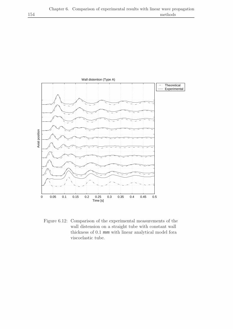
154Chapter 6. Comparison of experimental results with linear wave propagation
methods
0 0.05 0.1 0.15 0.2 0.25 0.3 0.35 0.4 0.45 0.5Time [s]
Axi
al p
ositi
on
Wall distention (Type A)
TheoreticalExperimental
Figure 6.12: Comparison of the experimental measurements of thewall distension on a straight tube with constant wallthickness of 0.1 mmwith linear analytical model foraviscoelastic tube.

6.6. Closure 155
0 0.05 0.1 0.15 0.2 0.25 0.3 0.35 0.4 0.45 0.5Time [s]
Axi
al p
ositi
on
Pressure P0 (Type B)
TheoreticalExperimental
(a)
0 0.05 0.1 0.15 0.2 0.25 0.3 0.35 0.4 0.45 0.5Time [s]
Axi
al p
ositi
on
Pressure P1 (Type B)
TheoreticalExperimental
(b)
Figure 6.13: Comparison of the experimental measurements of thepressure on a straight tube with constant wallthickness of 0.05 mmwith linear analytical model foraviscoelastic tube.

156Chapter 6. Comparison of experimental results with linear wave propagation
methods
0 0.05 0.1 0.15 0.2 0.25 0.3 0.35 0.4 0.45 0.5Time [s]
Axi
al p
ositi
on
Flow Q (Type B)
TheoreticalExperimental
Figure 6.14: Comparison of the experimental measurements of theflow on a straight tube with constant wall thicknessof 0.05 mmwith linear analytical model foraviscoelastic tube.
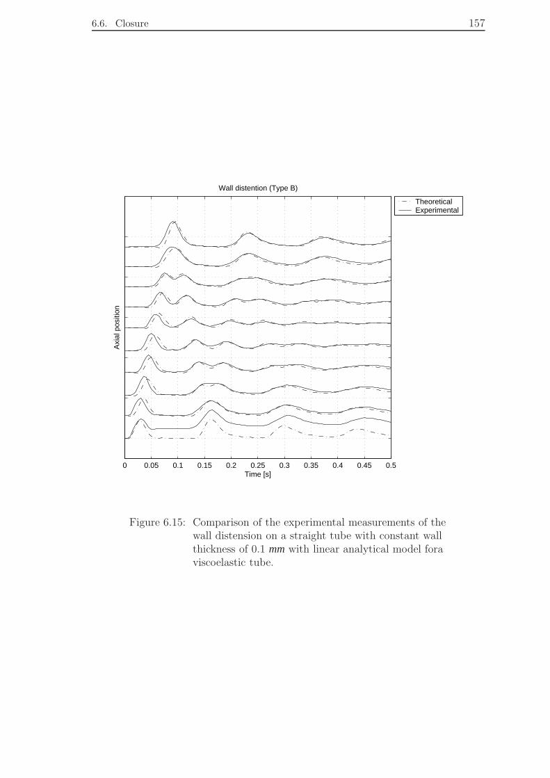
6.6. Closure 157
0 0.05 0.1 0.15 0.2 0.25 0.3 0.35 0.4 0.45 0.5Time [s]
Axi
al p
ositi
on
Wall distention (Type B)
TheoreticalExperimental
Figure 6.15: Comparison of the experimental measurements of thewall distension on a straight tube with constant wallthickness of 0.1 mmwith linear analytical model foraviscoelastic tube.

158Chapter 6. Comparison of experimental results with linear wave propagation
methods
viscoelastic. The experimental waveforms for pressure, flow and wall distension have
been compared with the theory. The pressure gradient has not been investigated as
it is expected to be in good agreement if the pressure comparisons are good.
The linear theory without viscoelasticity included cannot predict the pulse be-
haviour. The wave speed is well predicted by the linear theory as it can be seen from
the peak-to-peak comparisons of the experimental and computational data graphs.
However, the shape of the pulse after the first reflection at the distal end, is very
different. The amplitude of the pulse is highly overestimated as there is damping
only from the liquid.
Viscoelasticity is the most important parameter for the attenuation of the waves.
When the viscoelasticity of the material is included in the linear model, the match-
ing of the experimental measurements and the theoretical predictions is very good.
Therefore, we can conclude that that the tube is behaving in accordance to the linear
theory and the quality of the measurements is good. As a result it can be verified
that the findings of the previous chapter are valid.

Chapter 7
Conclusions
7.1 Overview
This thesis is concerned with the study of fluid-stucture interaction in flexible tubes
both from the modelling as well as the experimental point of view. More specifically,
it presents the first stage of development and testing of a novel unified solution
method suitable for fluid-structure interaction problems.
In Chapter 2, the mathematical description of the single solution method, was
derived. Fluid and solid were treated at as a continuum with different constitutive
equations for the stress tensor. The constitutive equation for a linear viscous New-
tonian fluid has as primitivevariables the velocity and the pressure, whereas for a
linear elastic solid the displacement. In order to develop a unified formulation, the
equation for the solid was altered in order to have velocity and pressure as primitive
variables. Thus, a single set of equations was obtained, with primitive variables
velocity and pressure. In the unified expression, the states of fluid and solid were
distinguished by different coefficients in the same equation. Thus, the fluid-solid
interface in the solution domain is internal and does not need special conditions for
the exchange of information between the two media, as it is inherently implicit.
In Chapter 3, the numerical method used for the solution of the equations was de-
scribed. Issues involving the convergence rate were addressed and taken into account
in the solution of the equations. The PISO velocity-pressure coupling algorithm used
was described. However, instead of solving for pressure corrections, it is used to solve
directly for pressure. This algorithm was used and tested for the first time in solid
dynamics. An extensive boundary condition investigation was presented that led
to the derivation of the optimal boundary conditions in a fully implicit velocity-
pressure solution of the Navier Stokes equations for a compressible material. A one
dimensional stability analysis was performed on the finite difference approximations
used for the displacement formulation and for the new velocity-based formulation.
In Chapter 4, the solution method for the reformulated equations for solids was
validated against the structural dynamic problem of beam bending, a case which
159
160 Chapter 7. Conclusions
incluses not only normal but also shear stresses. The results were compared against
the standard displacement formulation as well as with analytical solutions. For this
particular problem the analytical solutions have been obtained using simplifying as-
sumptions and this has to be taken into account when comparing analytical with
the numerical results. The conservation of the total energy of the numerical imple-
mentation was also tested. The numerical accuracy of the standard displacement
formulation was compared against the velocity based formulation. The dissipa-
tion characteristics of the numerical integration technique were also in agreement
with the conclusions obtained from the one dimensional stability analysis. Differ-
ent discretisation schemes were compared and the effect of the mesh resolution was
investigated. For the fully implicit velocity-pressure coupling, the successful use of
the optimal boundary conditions was illustrated. The optimal boundary conditions
were obtained for velocity by applying force balance at the free boundary and for
the pressure by projection of the momentum equation on the unit vector normal
to the boundary and solving for the normal pressure gradient. The novel solution
method was also validated for other beam bending cases with different dimensions.
In Chapter 5, experimental measurements in flexible vessels were presented that
can be used for the detailed validation of the unified approach. Six tubes were
manufactured: three straight and three tapered ones. One straight tube had wall
thickness variation such that the wave speed according to the linear theory would be
the same as in one of the tapered tubes. One tapered tube had variable wall thickness
such that the wave speed according to the linear theory would be the same as in
one of the straight tubes. The material properties of the tubes were measured by
relaxation tests. In the experiments performed, a pressure wave was initiated by
the opening of a valve. Pressure, pressure gradient, flow rate and wall distension
were measured simultaneously. The results from the different types of tubes were
compared against each other and the importance of the geometric tapering and wall
thickness variationin wave propagation were assessed.
Finally, in Chapter 6, the experimental data measured in the straight tubes
with constant wall thickness was compared with the one dimensional linear wave
propagation theory. Calculations for both elastic and viscoelastic material were
performed. The pressure, volumetric flow rate and wall distension propagation where
well reproduced by the linear theory when the viscoelastic properties of the wall were
taken into account.

7.2. Main achievements 161
7.2 Main achievements
This research has resulted in the following specific contributions:
• The idea of a unified solution methodology for solving fluid-structure inter-
action problems is presented. It is believed that the idea is general and can
be used to handle interaction between other continua which are described by
different constitutive equations. The interaction problems can be described
by a single set of equations in a single grid and, in this way the interface is
internal to the domain.
• The mathematical framework of the new method for fluid-structure interaction
problems has been developed. The method is fully implicit, three dimensional
and without simplifying assumptions. It is suitable for modelling a variety of
FSI applications such as pulse wave propagation in flexible tubes, container
impact etc.
• A numerical solution method for the discretisation and solution of the re-
formulated equations was also developed. The method is fully compatible
with the one currently used widely for the solution of the equations for fluids.
More specifically, for discretisation the finite volume approach is used and for
pressure-velocity coupling the PISO algorithm. It is the first time that this
algorithm is used for solving structural dynamic problems. The fact that the
reformulated equations have the same unknown variables as the ones for fluids
while the same numerical method can be used for their solution, greatly facil-
itates the implementation of a unified methodology for coupled FSI problems.
• Appropriate boundary conditions for the pressure equation were found for the
free boundary for compressible materials when a fully implicit velocity-pressure
method is used.
• The reformulated equations and solution method were successfully tested for
a structural dynamic problem (beam bending) that comprises both normal as
well as shear stresses.
• A complete experimental data set was produced that can be used for the next
step of the testing of the unified FSI approach. More specifically, the exper-
imental work focused on the effect of geometric tapering and wall thickness
variation on pulse wave propagation in flexible vessels. The experimental mea-
surements indicate that the tapering leads to higher pressure amplitude and
alters the shape of the pressure pulse.
• The classic wave propagation theory was used to simulate the aforementioned
experimental measurements for straight tubes with constant diameter and wall

162 Chapter 7. Conclusions
thickness. It was found that when the viscoelastic properties of the wall ma-
terial are included the predictions match well the experiments.
7.3 Future work
This thesis has covered a wide range of aspects in the area of fluid structure in-
teraction such as mathematical modelling and experiments. Therefore, the recom-
mendations for future work will be split into these categories and will be discussed
separately.
7.3.1 Mathematical modelling
Modelling an elastic material is quite restrictive as the materials in nature exhibit
viscoelastic properties. The mathematical model developed can be extended to in-
clude a simple viscoelastic model for the solid. Large deformations are also very
common in engineering practice, thus a arbitrary-Lagrangian-Eulerian large strain
formulation for the continuum can be introduced to take account for the large de-
formations typically occurring in the vessel walls.
The mathematical model presented here is quite general without approximations.
Thus it can be used for a number of disciplines. The important issue is that there
should be a genuine interaction between the fluid and the solid. Otherwise separate
solution methods would be more suitable.
The numerical model has been successfully validated against analytical solutions
to dynamic structural problems. The next step is to validate it for wave propagation
in tubes against the one dimensional linear wave theory presented in Chapter 6 of
this thesis. Validation of the new methodology on wave propagation in a flexible
tube was performed during the duration of this project and the results were very
promising. However, due to lack of time they were not investigated deeply enough
to be presented in this thesis.
However, it will be described here how the unified solution method can solve
a fluid-structure interaction problem. The single set of equations (momentum and
continuity) are describing the fluid-structure continuum are Equations 7.1 and 7.2.
∂ρ∂t
+∇ •(ρU) = 0 (7.1)
and
∂ρU∂t
+∇ •(ρUU) = 2αdev(sym(∇U))+φ∇ •devΣ+−∇p (7.2)
The state of the continuum is distinguished by different values the density ρ, the
constant α and phase constant φ (Equations 7.37.47.5).

7.3. Future work 163
φ = 1φ = 1 φ = 1φ = 1φ = 1
φ = 0φ = 0φ = 0φ = 0φ = 0
α = ηα = ηα = ηα = ηα = ηρ = ρ fρ = ρ fρ = ρ fρ = ρ fρ = ρ f
ρ = ρ f ρ = ρ f ρ = ρ f ρ = ρ f ρ = ρ fα = η α = η α = η α = η α = η
φ = 0φ = 0φ = 0φ = 0φ = 0
φ = 0 φ = 0 φ = 0 φ = 0 φ = 0
φ = 1 φ = 1 φ = 1 φ = 1φ = 1
ρ = ρs ρ = ρs ρ = ρs ρ = ρs ρ = ρs
ρ = ρsρ = ρsρ = ρsρ = ρsρ = ρs
ρ = ρ f ρ = ρ f ρ = ρ f ρ = ρ f ρ = ρ fα = η α = η α = η α = η α = η
α = µ∆t2α = µ∆t
2α = µ∆t2α = µ∆t
2α = µ∆t2
α = µ∆t2 α = µ∆t
2 α = µ∆t2 α = µ∆t
2 α = µ∆t2
NOTE: The coloured cells are in a solid state and the white cells are in a fluid state.
Figure 7.1: The different properties distribution in the single meshfor solving fluid structure interaction problems withthe unified solution method.
ρ =
{ρs f or solid
ρ f f or f luid(7.3)
α =
{µ∆t
2 f or solid
η f or f luid(7.4)
φ =
{1 f or solid
0 f or f luid(7.5)
In Figure 7.1 the schematic of how this is applied in a single grid is seen. There
is no exchange of information at the phase boundary between the two continua; the
interface is inherently implicit.
It would be very interesting to compare the unified solution method for solving
fluid structure interaction problems against monolithic methods to see if there is
reduction of computational time as it is expected. The solution accuracy comparison
of the two method will give a good guide for the future development.
This new way of solving solids in the same way as fluids can also be investi-
gated further by comparisons with standard stress analysis codes that use accurate
schemes of the discretisation. An error analysis together with a computational time
comparison could be performed to see if there are any benefits in using a velocity-
pressure formulation over a displacement formulation for solving solids outside the
fluid-structure interaction context.
When viscoelasticity is included in the mathematical model, the models can be

164 Chapter 7. Conclusions
validated both against the one dimensional theory with viscoelasticity included and
against the experimental data with real pressure boundary conditions at the entrance
taken from the measurements as presented in Chapter 6.
7.3.2 Experimental work
From the work presented Chapter 5 it was suggested that geometric tapering is
of great importance, as the constant reflections from the tapered wall change the
shape of the propagating wave, which cannot be predicted by the linear theory.
Comparison of this data with non linear theory would be of great interest.
The experimental measurements presented in Chapter 5 were obtained for small
deformations. The next step would be to repeat the same measurements with large
deformations and compare the results. This would further assist the understanding
of wave propagation in flexible vessels and would provide more validation data for
theoretical and numerical studies in the field. The ultrasound wall tracking system
can also measure shear rate. Thus, this measurement can be included.
The experiments presented in this thesis were obtained for a single type of initial
pulse. It would be interesting to conduct measurements with different types of
pulses. The most interesting would be to use a pulse that replicates the pulse from
the heart.
Bibliography
Abbott, M. B. and Basco, D. R. (1989). Computational fluid dynamics: an intro-
duction for engineers. Addison Wesley Longman, Essex, England.
Abe, H., Hayashi, K., and Sato, M. (1996). Data book on mechanical properties on
living cells, tissues and organs. Springer-Verlag, Tokyo, Japan.
Adams, A. A. (2003). Calculus: a complete course. Addison Wesley Longman,
Ontario, Toronto, Canada.
Alonso, J. and Jameson, A. (January 1994). Fully-implicit time-marching aeroelastic
solutions. 32nd AIAA Aerospace Sciences Meeting and Exhibit, Paper 94-0056,
American Institute of Aeronautics and Astronautics.
Anderson, D. A., Tannehill, J. C., and Pletcher, R. H. (1984). Computational fluid
mechanics and heat transfer. Hemisphere.
Aris, R. (1962). Vector, Tensors and the basic equations of fluid mechanics. Prentice-
Hall Inc., Englewood Cliffs, New Jersey.
Atabek, H. B. (1968). Wave propagation throught a viscous fluid contained in a
tethered, initially stressed, orthotropic elastic tube. Biophysical journal, 8:626–
649.
Atabek, H. B. and Chang, C. C. (1961). Oscillatory flow near the entry of a circular
tube. ZAMP, pages 185–201.
Atabek, H. B. and Lew, H. S. (1966). Wave propagation through a viscous incom-
pressible fluid contained in an initially stressed elastic tube. Biophysical journal,
6:481–503.
Bailey, C., Taylor, G. A., Cross, M., and Chow, P. (1999). Discretization procedures
for multi-physics phenomena. Journal of Computational and Applied Mathemat-
ics, 103:3–17.
Barnard, A. C. L., Hunt, W. A., Timlake, W. P., and Varley, E. (1966). A theory
of fluid flow in compliant tubes. Biophysical Journal, 6:717–724.
165

166 Bibliography
Bathe, K.-J. (1996). Finite element procedures. Prentice Hall, Englewood Cliffs,
New Jersey.
Bathe, M. and Kamm, R. D. (1999). A fluid-structure interaction finite element
analysis of pulsatile blood flow through a compliant stenotic artery. Journal of
Biomechanical Engineering - Transactions of the ASME, 121:361–369.
Belardinelli, E. and Cavalcanti, S. (1992). Theoretical analysis of pressure pulse
propagation in arterial vessels. Journal of Biomechanics, 25:1337–1349.
Belytschko, T., Karabin, M., and Lin, J. I. (1986). Fluid-structure interaction in
waterhammer response of flexible piping. ASME Journal of Pressure Vessel Tech-
nology, 108:249–255.
Bloom, F. J. (1998). A monolithical fluid-structure interaction algorithm applied
to the piston problem. Computer methods in applied mechanics and engineering,
167:369–391.
Brands, P. J., Hoeks, A. P. G., Willigers, J., and Willekes, C. (1999). An integrated
system for the non-invasive assesment of vessel wall and hemodynamic properties
of large arteries by means of ultrasound. European Journal of Ultrasound, 9:257–
266.
Burattini, R., Fogliardi, R., and Gobbi, R. (1996). Letter to the editor. comments on
’exponentially tapered t-tube model of systemic arterial system in dogs’. Medical
Engineering Physics, 18:333–335.
Caughey, D. A. and Hafez, M. M. (1994). Frontiers of computational flud dynamics
1994. John Wiley Sons Inc., West Sussex, UK.
Chadwick, P. (1976). Continuum mechanics concise theory and problems. George
Allen Unwin Ltd., Toronto, Ontario.
Chang, K. C., Tseng, Y. Z., Lin, Y. J., Kuo, T. S., and Chen, H. I. (1994). Ex-
ponentially tapered t-tube model of systemic arterial system in dogs. Medical
Engineering Physics, 16:370–378.
Cox, R. H. (1969). Comparison of linearized wave propagation models for arterial
blood flow analysis. Journal of Biomechanics, 2:251–265.
Demirdzic, I. and Z.Lilek, M. P. (1993). A collocated finite volume method for
predicting flows at all speeds. Int. J. Numer. methods Fluids, 16:1029–1050.
Demirdzic, I. and Martinovic, D. (1993). Finite volume method for thermo-elastic-
plastic stress analysis. Computer Methods in Applied Mechanics and Engineering,
109:331–349.

Bibliography 167
Demirdzic, I. and Muzaferija, S. (1994). Finite volume method for stress analysis in
complex domains. International Journal for Numerical Methods in Engineering,
37:3751–3766.
Demirdzic, I. and Muzaferija, S. (1995). Numerical method for coupled fluid flow,
heat transfer and stress analysis using unstructured moving meshes with cells of
arbitrary topology. Computer Methods in Applied Mechanics and Engineering,
125:235–255.
Deng, Q. H. and Tang, G. F. (2002). Special treatment of pressure correction
based on continuity conservation in a pressure-based algorithm. Numerical Heat
Transfer, 42:73–92.
Deters, O. J., Bargeron, C. B., Mark, F. F., and Friedman, M. H. (1986). Mea-
surement of wall motion and wall shear in a compliant arterial cast. Journal of
Biomedical Engineering ASME, 108:355–358.
Doormal, J. P. V., Raithby, G. D., and McDonald, B. H. (1987). The segregated
approach to predicting viscous compressible fluid flows. ASME Journal of Turbo-
machinery, 109:268–277.
Dutt, P. (1988). Stable boundary conditions and difference schemes for navier-stokes
equations. SIAM Journal on Scientific Computing, 25:245–267.
Dutta, A., Wang, D. M., and Tarbell, J. M. (1992). Numerical analysis of flow in an
elastic artery model. Journal of Biomechanical Engineering ASME, 114:26–33.
Dym, C. L. and Shames, J. (1970). Solid mechanics. McGraw-Hill Book Co, Tokio,
Japan.
Einav, S., Aharoni, S., and Manoach, M. (1988). Exponentially tapered transmission
line model of the arterial system. IEEE Transactions on Biomedical Eingineering,
35:333–339.
Farhat, C., Lesoinne, M., and Tallec, P. L. (1998). Load and motion transfer al-
gorithms for fluid/structure interaction problems with non-marching discrete in-
terfaces: momentum and energy conservation optimal discretisation and applica-
tion to aeroelasticity. Computer methods in applied mechanics and engineering,
157:95–114.
Farhat, C., Pieterson, K., and Degand, D. (2001). Multidisciplinary simulation of
maneuvering of an aircraft. Engineering with computers, 17:16–27.
Felippa, C. A., Park, K. C., and Farhat, F. (2001). Partitioned analysis of coupled
mechanical systems. Computer methods in applied mechanics and engineering,
190:3247–3270.

168 Bibliography
Ferziger, J. H. and Peric, M. (1996). Computational methods for fluid dynamics.
Springer-Verlag, Berlin, Germany.
Fogliardi, R., Burrattini, R., and Campbell, K. B. (1997). Identification and phys-
iological relevance of an exponentially tapered tube of canine descending aortic
circulation. Med. Eng. Phys., 19:201–211.
Fung, Y. C. (1997). Biomechanics: Circulation. Springer-Verlag, New York, USA.
Geradin, M. and Rixen, D. (1997). Mechanical Vibrations: theory and application
to structural dynamics. John Wiley Sons Inc., New York, USA.
Gerrard, J. H. (1985). An experimental test of the theory of waves in fluid-filled
deformable tubes. J. Fluid Mech., 156:321–347.
Giannopapa, C. G. (May 2002). Fluid structure interaction in flexible vessels. Trans-
fer report from MPhil to PhD, Kings College London, University of London.
Girault, V. and Raviart, P. A. (1986). Finite element methods for Navier-Stokes
equations. Springer, Berlin, Germany.
Greenshields, C. J., Weller, H. G., and Ivankovic, A. (1999). The finite volume
method for coupled fluid flow and stress analysis. Computer Modeling and Simu-
lation in Engineering, 4:213–218.
Gresho, P. H. and Sani, R. L. (1987). On pressure boundary conditions for the incom-
pressible navier-stokes equations. International Journal for Numerical Methods in
Fluids, 7:1111–1145.
Gresho, P. M. and Sani, R. L. (2000). Incompressible flow and the finite element
method, 2 volume set. John Wiley Sons Inc., West Sussex, UK.
Gustafsson, B. and Sundstrom, A. (1978). Incompletely parabolic problems in fluid
dynamics. SIAM Journal on Scientific Computing, 35:343–357.
Hageman, L. A. and Young, D. M. (1981). Applied iterative methods. Academic
Press, New York.
Henry, F. S. and Collins, M. W. (1993a). A novel predictive model with compliance
for arterial flow. Advances in Bioengineering — American Society of Mechanical
Engineers, BED 26:131–135.
Henry, F. S. and Collins, M. W. (1993b). Prediction of transient wall movement
of an incompressible elastic tube using a finite volume procedure. Computational
Biomedicine, 26:165–172.

Bibliography 169
Hesthaven, J. S. (1997). A stable penalty method for the compressible navier-stokes
equations. ii. one-dimentional domain decomposition schemes. SIAM Journal on
Scientific Computing, 18:658–685.
Hesthaven, J. S. and Gottlieb, D. (1996). A stable penalty method for the com-
pressible navier-stokes equations. i. open boundary condisions. SIAM Journal on
Scientific Computing, 3:579–612.
Higham, D. J. (2000). Mean-square and asymptotic stability of the stochastic theta
method. SIAM Journal of Numerical Analysis, 38:753–769.
Hirsch, C. (1988). Numerical computation of internal and external flows. Wiley,
Chichester, UK.
Hoeks, A. P. G., Willekes, C., Bourouyrie, P., Brands, P. J., Willigers, J. M., and
Reneman, R. S. (1997). Automated detection of local artey wall thickness based
on m-line signal processing. Ultrasound in Med. & Biol., 23:1017–1023.
Horsten, J. B. A. M., van Steenhoven, A. A., and van Dongen, M. E. H. (1989). Lin-
ear propagation of pulsatile waves in viscoelastic tubes. Journal of Biomechanics,
22:477–484.
Hubner, B., Walhorn, E., and Dinkler, D. (2004). A monolithic approach to fluid-
structure interaction using space-time finite elements. Computer methods in ap-
plied mechanics and engineering, 193:2087–2104.
Hughes, T. J. R. (1987). The Finite Element Method: linear static and dynamic
finite element analysis. Dover Publications,Inc., Mineola, New York.
Issa, R. I. (1986). Solution of the implicitly discretised fluid flow equations by
operator-splitting. Journal of Computational Physics, 62:40–65.
Jasak, H. and Weller, H. G. (2000). Application of the finite volume method and un-
structured meshes to linear elasticity. International Journal for Numerical Meth-
ods in Engineering, 48(2):267–287.
Klip, W. (1962). Velocity and damping of pulse wave. Martinus Nijhoff, The Hague,
Netherlands.
Klip, W., Loon, P. V., and Klip, D. A. (1968). Formulas for phase velocity and
damping of longitudinal waves in thick-walled, viscoelastic tubes. Journal of ap-
plyed Physics, 38:3745–3755.
Konig, C. S., Clark, C., and Mokhtarzaden-Dehgham, M. R. (1999). Comparison
of fluid in numerical and physical models of a ventricular assist device using low-
and high-viscosity fluids. Journal of Biomedical Engineering, 116:294–301.

170 Bibliography
Korteweg, D. J. (1878). Uber die Fortplanzungsgeschwindigkeit des Schalles in
elastischen rohren (on the velocity of propagation of sound in elastic pipes.). An-
nalen der Physik und Chemie, 5:525–542.
Ku, D. N., Biancheri, C. L., Pettigrew, R. I., W.Peifer, J., Markou, C. P., and
Engels, H. (1990). Evaluation of magnetic resonance velocimetry for steady flow.
ASME Journal of Biomechanical Engineering, 112:464–472.
Levick, J. R. (2000). Cardiovascular physiology. Arnold, London, UK.
Liepsch, D. and Moravec, S. (1984). Pulsatile flow of non-newtonian fluid in disten-
sible models of human arteries. Biorheology, 21:571–586.
Lighthill, J. (1975). Mathematical biofluiddynamics : a treatment in bookform of the
material in the lecture course delivered to the research conference of the National
Science Foundation, held July 1973 at Rensselaer Polytechnic Institute, Troy,
New.York. Society for Industrial and Applied Mathematics, Philadelphia, Pa,
USA.
Lighthill, J. (1978). Waves in fluids. Cambridge University Press, Cambridge, UK.
Ling, S. C. and Atabek, H. B. (1972). A nonlinear analysis of pulsatile flow in
arteries. Journal of Fluid Mechanics, 55:493–511.
Malvern, L. E. (1969). Introduction to the Mechanics of a Continuous Medium.
Prentice-Hall Inc., Englewood Cliffs, New Jersey.
Mattheij, R. M. M., Rienstra, S. W., and ten Thije Boonkkamp, J. H. M. (2005).
Partial differential equations: modelling, analysis and computing. SIAM, Philadel-
phia (in press).
McDonald, D. A. (1968). Blood flow in arteries. Arnolds, London.
Mirsky, I. (1968). Wave propagation in a viscous fluid contained in an orthotropic
elastic tube. Biophysical Journal, 7:165–186.
Moens, A. I. (1878). Die pulscurve. E. J. Brill, Leyden, The Netherlands.
Moin, P. and Kim, J. (1980). On the numerical solution of time-dependent viscous
incompressible fluid flows involving solid boundaries. Journal of Computational
Physics, 3:381–392.
Nabla, L. (23rd April 2002). Programmers guide. Version 2.1.
Nerem, R. M., Seed, W. A., and Wood, N. B. (1971). An experimental study of the
velocity distribution and transition to turbulence in the aorta. J. Fluid Mech.,
52:137–160.

Bibliography 171
O.Ladyshenkaya (1998). Mathematical problems in the dynamics of viscous incom-
pressible fluids. Gordon and Breach, New Yourk, USA.
Olivier, J. and Sundstrom, A. (1978). Theoretical and practical aspects of some
initial boundary value problems in fluid dynamics. SIAM Journal on Scientific
Computing, 35:419–446.
Orszag, S. and Israeli, M. (1974). Numerical simulation of viscous incompressible
flows. Annual Review of Fluid Mechanics, Paolo Alto, CA, pages 281–319.
Patankar, S. V. (1980). Numerical heat transfer and fluid flow. McGraw-Hill, New
York.
Patankar, S. V. and Spalding, D. B. (1972). A calculation procedure for heat, mass
and momentum transfer in three-dimensional parabolic flows. Int. J. Heat Mass
Trans., 15:1787–806.
Pedley, T. J. (1980). The fluid mechanics of large blood vessels. Cambridge Univer-
sity Press, Cambridge, UK.
Perktold, K. and Rappitsch, G. (1995). Computer simulation of local blood flow
and vessel mechanics in a compliant carotid artery bifurcation model. Journal of
Biomechanics, 28:845–856.
Rade, L. and Westergren, B. (1990). Beta mathematics handbook. CRC Press, 2nd
Edition.
Raveh, D. (September 2000). Reduced order models for nonlinear unsteady aero-
dynamics. 8th AIAA/USAF/NASA/ISSMO Symposium on Multidisciplinary
Analysis and Optimization, Long Beach, CA. American Institute of Aeronautics
and Astronautics.
Reuderink, P., Sipkema, P., and Westerhof, N. (1988). Influence of geometric taper
on the derivation of the true propagation coefficient using a three point method.
Journal of Biomechanics, 21:141–153.
Reuderink, P. J., Hoogstraten, H. W., Sipkema, P., Hillen, B., and Westerhof, N.
(1989). Linear and nonlinear one-dimensional models of pulse wave transmission
at high Womersley numbers. Journal of Biomechanics, 22:819–827.
Reuderink, P. J., van de Vosse, F. N., van Steenhoven, A. A., van Dongen, M. E. H.,
and Janssen, J. D. (1993). Incompressible low-speed-ratio flow in non-uniform
distensible tubes. Journal of Numerical method in Fluids, 16:597–612.

172 Bibliography
Rhie, C. M. and Chow, W. L. (1982). A numerical study of the turbulent flow past
an isolated airfoil with trailing edge separation. AIAA-82-0998, AIAA/ASME 3rd
Joint Thermophysics, Fluids, Plasma and Heat Transfer Conference, St. Louis,
Missouri.
Rifai, S. M., Johan, Z., Wang, W. P., Grisval, J. P., Hughes, T. J. R., and Ferencz,
R. M. (1998). Multiphysics simulation of flow-induced vibrations and aeroelastic-
ity on parallel computing platforms. Computer methods in applied mechanics and
engineering, 174:394–417.
Roades, R. A. and Tanner, G. A. (1995). Medical physiology. Lippincott Williams
Wilkins, Baltimore, USA.
Rutten, M. C. M. (1998). Fluid-solid interaction in large arteries. PhD thesis,
University of Eindhoven.
Segel, L. A. (1977). Mathematics applied to continuum mechanics. Macmillan Pub-
lishing Co., New York, USA.
Slone, A. K., Bailey, C., and Cross, M. (2003). Dynamic solid mechanics using finite
element methods. Applied mathematical modelling, 27:69–87.
Steinman, D. A. and Ethier, C. R. (1994). The effect of wall distensibility on flow in
a two-dimensional end-to-side anastomosis. Journal of Biomechanical Engineering
- Transactions of the ASME, 116:294–301.
Streeter, V. L. and Wylie, E. B. (1979). Fluid mechanics. McGraw-Hill, New York.
Tallec, P. L. and Mouro, J. (2001). Fluid structure interaction with large struc-
tural displacements. Computer methods in applied mechanics and engineering,
190:3039–3067.
Tang, D., Yang, C., Huang, Y., and Ku, D. N. (1999a). Wall stress and strain
analysis using a 3-D thick-wall model with fluid-structure interactions for blood
flow in carotid arteries with stenoses. Computers and Structures, 72:341–356.
Tang, D., Yang, C., and Ku, D. N. (1999b). A 3-D thin-wall model with fluid-
structure interactions for blood flow in carotid arteries with symmetric and asym-
metric stenoses. Computers and Structures, 72:357–377.
Taylor, C. A., Hughes, T. J. R., and Zarins, C. K. (1998). Finite element model-
ing of blood flow in arteries. Computational Methods in Applied Mechanics and
Engineering, 158:155–196.
Taylor, M. G. (1965). Wave travel in a non-uniform transmission line, in relation to
pulses in arteries. Physics in Medicine and Biology, 10:539–550.

Bibliography 173
Tijsseling, A. S. (1996). Fluid-structure interaction in liquid-filled pipe systems: a
review. Journal of Fluids and Structures, 10:109–146.
Tijsseling, A. S. and Wiggert, D. C. (2001). Fluid transients and fluid-structure
interaction in flexible liquid-filled piping. American Society of Mechanical Engi-
neers, 54:455–481.
Timoshenko, S. P. and Goodier, J. N. (1970). Theory of elasticity. McGraw-Hill
Book Co, Singapore.
Turner, M. J., Clough, R. W., Martin, H. C., and Topp, L. J. (1956). Stiffness and
deflection analysis of complex structures. Journal of Aerospace Science, 23:805–
833.
Ugural, A. C. and K.Fenster, S. (2003). Advanced strength and applied elasticity.
McGraw-Hill Book Co, New Jersey, USA.
van Brummelen, E. H., Hulshoff, S. J., and de Borst, R. (2003). Energy conservation
under incompatibility for fluid-structure interaction problems. Computer methods
in applied mechanics and engineering, 192:2727–2748.
van Brummelen, E. H. and Koren, B. (2003). A pressure-invariant conservation
godunov-type method for barotropic two-fluid flows. Journal of Computational
Physics, 185:289–308.
van Steenhoven, A. A. and van Dongen, M. E. H. (1986). Model studies of the aortic
pressure rise just after value closure. Journal Fluid Mechanichs, 166:93–113.
Versteeg, H. K. and Malalasekera, W. (1995). Computational fluid dynamics. The
finite volume method. Prentice Hall, Essex, UK.
von Kries, J. (1883). Uber die beziehungen zwischen druck und geschwindigkeit,
welche bei der wellenbewegung in elestischen schlauchen bestehen. Festschrift der
56. Versammlung deutscher Naturforscher und Arzte gewidmet von der Natur-
forschenden Gesellschaft zu Freiburg i. B., Supplement zu Band VIII der Berichte
uber die Verhandlungen der Naturforschenden Gesellschaft zu Freiburg i. B.,
Akademische Verlagsbuchhndlung vor JCB Mohr (Paul Siebeck), Freibung im
Breisgau und Tubingen, Germany, 67-88.
von Kries, J. (1892). Studien zur Pulslehre. PhD thesis, Akademische Verlagsbuch-
handlung von JCB Mohr (Paul Siebeck).
Weller, H. G., Tabor, G., Jasak, H., and Fureby, C. (1998). A tensorial approach
to continuum mechanics using object-oriented techniques. Computers in Physics,
12:620–631.

174 Bibliography
Wemple, R. R. and Mockros, L. F. (1972). Pressure and flow in the systemic arterial
system. Journal of Biomechanics, 5:629–641.
Westerhof, N., Bosman, F., Vries, C. J. D., and Noordergraaf, A. (1969). Analogue
studies of the human systemic arterial tree. Journal Biomechanics, 2:121–143.
Wilkins, M. L. (1964). Calculations of elastic-plastic flow. Methods in Computational
Physics, 3:211–263.
Witzig, K. (1914). Uber erzwungene wellenbegungen zaher, inkopressible flussigkeit-
edn in elastischen rohren. PhD theses, University of Bern.
Womersley, J. R. (1957). An elastic tube theory of pulse transmission and oscillatory
flow in mammalian arteries. Technical report, Wright Air Development Centre
TR56-614.
Wood, N. B. (1999). Aspects of fluid iynamics to the larger arteries. Journal of
Theoritical Biology, 199:137–161.
Wylie, E. B. and Streeter, V. L. (1993). Fluid transients in systems. Prentice Hall,
Englewood Cliffs, New Jersey.
Xu, X. Y., Long, Q., Collins, M. W., Bourne, M., and Griffith, T. M. (1999). Recon-
struction of blood flow patterns in human arteries. Proceedings of the Institution
of Mechanical Engineers Part H, 213:411–421.
Young, T. (1808). Hydraulic investigations, subservient to an intended croonian
lecture on the motion of blood. Philosophical Transactions of the Royal Society
(London), 98:164–186.
Zhao, S. Z., Xu, X. Y., and Collins, M. W. (1998). The numerical analysis of
fluid-solid interactions for blood flow in arterial structures. Part 2: development
of coupled fluid-solid algorithms. Proceedings of the Institution of Mechanical
Engineers Part H, 212:241–252.
Zienkiewcz, O. C. and Taylor, R. L. (1989). The finite element method, solid and
fluid mechanics. Dynamics and non-linearity., volume 5. McGraw-Hill, New York.
Zienkiewcz, O. C. and Taylor, R. L. (1991). The finite element method., volume 2.
McGraw-Hill, London.

Appendix A
The Tube Models Manufacturing
Methodology
In Section 1.4 it was presented the lack in the literature of well defined experiments
assessing the non-linearities of flexible vessels i.e. wall thickness variation and geo-
metric tapering. In order to obtain a complete set of experimental data assessing
these variations, a set of flexible tubes was manufactured.
A.1 The vessels design and specifications
The tubes were designed to be model analogues of the human aorta. One of the most
referenced sources of arterial dimensions is the one from Westerhof et al. (1969). In
Table A.1, the data mentioned in his work are presented and is used as a guidance
for the design of the tubes used in this work.
Variable Aorta Thoracalis
Top internal radius [mm] 20Bottom internal radius[mm] 11
Length [mm] 315Slope -0.014
ϒ∗h/D [MPa] 0.02-0.04
ϒ : Youngs modulus, h: wall thickness, D: internal diameter
Table A.1: Aorta anatomical data (Westerhof et al., 1969).
In order to be able to assess the effects of morphological variations in wave
propagation, six tubes were manufactured: three straight ones and three tapered
ones. The geometrical parameters of these tubes are summarised in Table A.3. It
should be mentioned that the tube of Type E has the same ϒ ∗ h/D as the aorta
according to Westerhof et al. (1969) (See Table A.1).
i

ii A.1. The vessels design and specifications
In order to be able to separate effects due to geometric tapered from the six
tubes, two pairs of tubes were manufactured in a specific manner, so that they
would have the same wave speed throughout according to linear theory. The first
pair consists of a geometrically tapered tube with constant wall thickness (Type
E) and a straight tube with variable wall thickness (Type C). The variable wall
thickness of the tube was designed so as according to linear theory the wave speed
throughout this straight tube will be the same as the tapered one with constant wall
thickness. The second pair consists of a straight tube with constant wall thickness
(Type A) and a tapered tube with variable wall thickness (Type F). The variable
wall thickness of the tapered tube was chosen such that according to linear theory
the wave speed throughout its length is the same as for a tapered tube with constant
wall thickness. In this way the variable wall thickness of the tapered tube according
to the linear theory will counterbalance the effect of geometric tapering.
Type D[mm] h±0.002[mm] L[mm] z ϒ∗h/D[MPa] c[m/s]
A 25 0.1 446 0 0.04 6.3
B 25 0.05 446 0 0.02 4.5
C 25 0.05-0.1 446 0 0.02-0.04 4.5-6.3
D 25-12.5 0.1 446 -0.014 0.04-0.08 6.3-8.9
E 25-12.5 0.05 446 -0.014 0.02-0.04 4.5-6.3
F 25-12.5 0.1-0.05 446 -0.014 0.04 6.3
ϒ: Young’s modulus, h: wall thickness, D: diameter
Table A.3: Geometrical parameters of tubes manufactured.

A.2. Manufacturing set-up iii
A.2 Manufacturing set-up
The tubes were manufactured by the method of spin coating. The set-up is shown
in Figure A.1. The tube will take the shape of a steel rod that can rotate along its
length axis through a servomotor (x-servomotor). The process can be seen in Figure
A.2.
The liquid used in the spin coating process is delivered through a nozzle that has
cross sectional area of 7mm2(π∗(3mm/2)2) and is injected by a pump. The pump can
operate only on constant flow rate throughout the process. The nozzle is attached
on a trolley that can translate along the length of the rod through by a rotating
ball screw rod connected to a second servomotor (y-servomotor). Different nozzles
designs were tried and optimal shapes were found by trial and error. As the trolley
translates the nozzle places a spiral stripe of resin of about 3 mm thickness on the
rotating rod. Under infrared light the liquid stripes will blend into each other and
solidify, creating a tube of certain thickness. The thickness of the tube is marginally
small, therefore two things are important for the consecutive spiral stripes to merge:
the positioning of the nozzle and the distance ξ between the stripes that should not
exceed 3 mm.
The x-servomotor rotates at Crot = 2000counts/revolution and has a 1-1 relation-
ship with the connected rotating beam. The y-servomotor rotates at Ctrans = 4000
counts/revolution and the ball screw pitch is λ = 2.5mm. Thus, the rotational move-
ment of 1600 counts the y-servomotor can be translated to translational movement
of 1 mm of the trolley. The translational movement of the y-servomotor is responsi-
ble for the thickness h of the tube and the rotational movement of the x-servomotor
is responsible for the spacing ξ between consequent raisin spirals delivered by the
nozzle.
The movement of the servo-motors can be controlled via an DMC-630 Galil
controller connected to a PC. In the following three sections the equations used for
the programming of the servomotors movement will be derived.
A.3 Equations for manufacturing
The following equations describing the behaviour of the machine regarding the tube
specifications have been written out and have been used for the programming of the
microcontroller.
Volume of straight tube
VL = πD(x)∗X ∗h∗100/α , xε [0,X] (A.1)
where D is the diameter of the steel rod, h is the thickness of the tube, X is the

iv A.3. Equations for manufacturing
x-servomotornozzletrolley with
infraredlight
steel rod
y-servomotor
λ
Figure A.1: Spin coating set-up ( TU/e).
ξ
Figure A.2: Spin coating process of a tube.

A.4. Straight tube manufacturing v
length of the rod and α is the concentration of the solution.
Volume of a tapered tube (Rade and Westergren, 1990)
V1 =π∗X12
[D(0)2+D(0)∗D(X)+D(X)2] , xε [0,X] (A.2)
V2 =π∗X12
[D(0)+d)2 +(D(0)+d)∗ (D(X)+d)+ (D(X)+d)2] , xε [0,X] (A.3)
VL = (V2−V1)∗100/α (A.4)
The horizontal to vertical slope of the cone is given by Equation A.5.
z=1
2X(D(X)−D(0)) (A.5)
Flow rate
FL =VL
t(A.6)
Frequency of servomotor rotation
f (x) =U(x)∆x
(A.7)
From the definition of frequency a relationship between the speed and the number
of counts per revolution (C) for the servo-motors can be obtained:
U(x) = C∗ f (x) (A.8)
For the x-servomotor Crot = 2000counts/revolution and for y-servomotor Ctrans=
4000counts /revolution.
A.4 Straight tube manufacturing
The specifications of the steel rod used as a manufacturing mould can be seen in
Figure A.3, and the straight tube specifications can be seen in Table A.5).
Variable Abbreviation Value
Diameter[mm] D 25Length [mm] X 500
Thicknes [mm] h(x) 0.05-0.1
Table A.5: Straight tube specifications.

vi A.4. Straight tube manufacturing
2.5 [cm]
50 [cm]
Figure A.3: Straight tube steel rod dimensions.
A.4.1 Constant thickness
The equations necessary for the manufacturing of the straight tube are Equations
A.1, A.6 and A.8. In order for the spiral liquid stripe of the solution to merge and
solidify homogeneously the distance between the spiral lines should be 0.2 ≤ ξ ≤0.3 [mm]. The rotational rotor is responsible for the spacing distance ξ, therefore in
Equation A.7 should have ∆x = ξ. So, its velocity in counts/s is:
Urot =FL ∗α/100h∗π∗D
Crot
ξ(A.9)
The equation giving the axial velocity of the y-servomotor in counts/secis given
by:
Uax =FL ∗α/100h∗π∗D
Cax
λ(A.10)
The relationship between the velocities of the two servo-motors is linear and
always valid regardless of the type of tube to be manufactured. Therefore it is
written in a general form at any point x along the length of the rod:
Urot(x) = Uax(x)Crot
Cax
λξ
(A.11)
A.4.2 Variable thickness
A tube with variable thickness is needed as described in Section A.1. The thickness
of the tube will be varying in a way that the wave velocity inside the tube at all time
will be the same as the wave velocity in a tapered tube with constant wall thickness
according to Moens Korteweg equation.
Considering a tapered tube with constant wall thickness h∗ , diameter varying
with the the rod length D∗(x) and varying wave speed c∗(x). The wave velocity is
give by
c∗(x) =
√ϒρ
h∗
D∗(x)(A.12)

A.4. Straight tube manufacturing vii
The straight tube with constant diameter D will have a varying wall thickness
with the rod length h(x) and a varying wave speed c(x). Thus, the wave velocity is
given by
c(x) =
√ϒρ
h(x)D
(A.13)
In order to have at all points along the length of the two tubes the same wave
velocity the two wave speeds should be the same at all times c(x) = c∗(x). Substitut-
ing Equations A.12 and A.13 the relationship according to which the wall thickness
should be varying is obtained.
h(x) =h∗ ∗DD∗(x)
(A.14)
The velocities of the x-servomotor and the y-servomotor can be given by sub-
stituting Equation A.14 in Equations A.9 and A.10. In Figure A.4 one can see the
wall thickness variation in relation to the tube length.
0 10 20 30 403000
4000
5000
6000
7000
Rod length [cm]
Tra
nsla
tiona
l Vel
ocity
[cou
nts/
sec]
0 10 20 30 402000
2500
3000
3500
4000
4500
Rod length [cm]
Rot
atio
nal V
eloc
ity [c
ount
s/se
c]
0 10 20 30 405
6
7
8
9
10x 10
−3
Rod length [cm]
Thi
ckne
ss [c
m]
0 10 20 30 401.5
2
2.5
3
3.5
Rod length [cm]
Rod
dia
met
er [c
m]
Figure A.4: Translational velocity, rotational velocity, tube wallthickness and tube diameter versus the tube lengthfor tube C.

viii A.5. Tapered tube manufacturing
A.5 Tapered tube manufacturing
For the manufacturing of the tapered tube a tapered steel bar was constructed
(FigureA.5) with dimensions shown in Table A.7. The equations describing this
requirements can be derived as follows.
A.5.1 Constant thickness
Using Equation A.5 the radius at any point x along the tapered bar is increasing
according to Equation A.15.
D(x) = D(0)−2x∗z , xε [0,X] (A.15)
Rewriting Equation A.15 in ∆x increments, Equation A.16 is obtained.
D(x) = D(x−∆x)−2∆x∗z , xε [0,X] (A.16)
1.25 [cm]
4 [cm] 44.6 [cm] 2.4 [cm]
2.5 [cm]
Figure A.5: Tapered tube steel rod dimensions.
Variable Abbreviation Value
Diameter at bottom [mm] D(0) 12.5Diamerter at top [mm] D(X) 25
Length [mm] X 446Horizontal to vertical slope z 0.014
Thickness [mm] h 0.05-0.1
Table A.7: Tapered tube specifications.
In the same way the equations giving the change in volume of the tube for every
increment ∆x is given by EquationsA.17, A.18, A.19 and A.20.
∆V1(x) =π∗∆x
12
[D(x)2+D(x)∗D(x+∆x)+D(x+∆x)2] , xε [0,X] (A.17)

A.5. Tapered tube manufacturing ix
∆V2(x) =π∗∆x
12
[(D(x)+h)2+(D(x)+h)∗ (D(x+∆x)+h)+(D(x+∆x)+h)2] , xε [0,X]
(A.18)
∆VL(x) = [∆V2(x)−∆V1(x)]∗100/a (A.19)
VL(x) =x=X
∑x=0
∆VL(x)∗100/α (A.20)
Substituting for time increments ∆t = ∆x/U(x) in EquationA.6, the velocity of
the trolley and the velocity of the rotating beam is given by:
Urot(x) =FL ∗∆x∆VL(x)
Crot
ξ(A.21)
Uax(x) =FL ∗∆x∆VL(x)
Cax
λ(A.22)
From Equations A.22, A.21 and EquationA.6 it can be seen that the relationship
between the distance along the bar and the translational velocity is non linear of
hyperbolic form.
The way of calculating the volume of the liquid described above is accurate using
the theory for a cone cylinder and can be used to calculate accurately the total
volume of the liquid that needs to be injected by the pump. For the programming
of the microcontroller and the calculation of the speed of the x, y-servo-motors the
volume of the stripe can be approximated by Equation A.1, where the diameter is
given by Equation A.15:
∆VL(x) = π∗D(x)∗∆x∗h∗100/α (A.23)
Therefore, by substituting Equation A.23 in Equations A.21 and A.22 the rota-
tional and axial velocities in counts/secare give by:
Urot =FL ∗α/100h∗π∗D(x)
Crot
ξ(A.24)
Uax =FL ∗α/100h∗π∗D(x)
Cax
λ(A.25)
For the update of the diameter a relationship is needed between ∆x and ∆t is
needed and can be obtained by substituting Equation A.23 in Equation A.6. One of
the two will have to be fixed and chosen arbitrary and the other will get calculated.
In Figure A.6 one can see the servo-motors hyperbolic velocity variation according
to the diameter change of the tube.

x A.5. Tapered tube manufacturing
0 10 20 30 40
5000
6000
7000
8000
9000
Rod length [cm]
Tra
nsla
tiona
l Vel
ocity
[cou
nts/
sec]
0 10 20 30 402500
3000
3500
4000
4500
5000
5500
6000
Rod length [cm]
Rot
atio
nal V
eloc
ity [c
ount
s/se
c]
0 10 20 30 400
0.002
0.004
0.006
0.008
0.01
Rod length [cm]
Tub
e th
ickn
ess
[cm
]
0 10 20 30 40
1.4
1.6
1.8
2
2.2
2.4
2.6
2.8
Rod length [cm]
Rod
dia
met
er [c
m]
Figure A.6: Translational velocity, rotational velocity, tube wallthickness and tube diameter versus the tube lengthfor tube E.

A.6. Wall thickness accuracy xi
A.5.2 Variable thickness
A tapered tube with variable thickness is needed as described in Section A.1 in order
to distinguish which effects are due to the geometric tapering. The thickness of the
tube will be varying in a way that the wave velocity inside the tube at all time will
be constant as it is in the straight tube with constant wall thickness according to
Moens Korteweg equation.
Considering a straight tube with constant wall thickness h∗, diameter D∗ and
constant wave speed c∗. The wave velocity is given by
c∗ =
√ϒρ
h∗
D∗ (A.26)
Considering a tapered tube with variable wall thickness h(x) , diameter varying
with the the rod length 12.5≤ D(x) ≤ 25 mm and constant wave speed c. The wave
velocity is give by
c =
√ϒρ
h(x)D(x)
(A.27)
In order to have at all points along the length of the two tubes the same constant
wave velocity the two wave speeds should be the same c= c∗. Thus, from Equations
A.26 and A.13 the relationship according to which the wall thickness should be
varying is obtained:
h(x) =h∗
D∗D(x) (A.28)
In Figure A.7 one can see the wall thickness variation 0.05≤ h(x) ≤ 0.1 mm in
relation to the tube length which is a linear relationship. The velocities of the x and
y-servo-motors can be obtained by substituting Equation A.28 in Equations A.24
and A.25.
A.6 Wall thickness accuracy
The wall thickness of the tubes manufactured was measured every 10 mm along the
tube length with a micrometer and it was found that the wall thickness accuracy
was ±2µm. This variation is small. Thus, for modelling purposes can be neglected.

xii A.6. Wall thickness accuracy
0 10 20 30 402000
4000
6000
8000
10000
12000
14000
16000
Rod length [cm]
Tra
nsla
tiona
l Vel
ocity
[cou
nts/
sec]
0 10 20 30 402000
4000
6000
8000
10000
Rod length [cm]
Rot
atio
nal V
eloc
ity [c
ount
s/se
c]
0 10 20 30 405
6
7
8
9
10x 10
−3
Rod length [cm]
Thi
ckne
ss [c
m]
0 10 20 30 40
1.4
1.6
1.8
2
2.2
2.4
2.6
2.8
Rod length [cm]
Rod
dia
met
er [c
m]
Figure A.7: Translational velocity, rotational velocity, tube wallthickness and tube diameter versus the tube lengthfor tube F.