Final Technical Report ESMART Subtask 5.8: Mechanical ... · Final Technical Report ESMART Subtask...
284
Final Technical Report ESMART Subtask 5.8: Mechanical Performance of Dies Award Number DE‐FC36‐04GO14230 Co‐Op Agreement No. 2005‐307 OSURF Project Number 746200 Project Period: January 2004 – June 2011 R. Allen Miller, Principal Investigator Phone: 614‐581‐1754 Email: [email protected] Ohio State University 210 Baker Systems Engineering 1971 Neil Ave. Columbus, OH 43210 Contributors: Khalil Kabiri‐ Bamoradian, Research Engineer Abelardo Delgado‐Garza, PhD Student Karthik Murugesan, PhD Student Adham Ragab, Postdoctoral Researcher Partner Organization: North American Die Casting Association September 13, 2011
Transcript of Final Technical Report ESMART Subtask 5.8: Mechanical ... · Final Technical Report ESMART Subtask...
Final Technical Report
ESMART Subtask 5.8: Mechanical Performance of Dies
Award Number DE‐FC36‐04GO14230
Co‐Op Agreement No. 2005‐307
OSURF Project Number 746200
Project Period: January 2004 – June 2011
R. Allen Miller, Principal Investigator
Phone: 614‐581‐1754
Email: [email protected]
Ohio State University
210 Baker Systems Engineering
1971 Neil Ave.
Columbus, OH 43210
Contributors:
Khalil Kabiri‐ Bamoradian, Research Engineer
Abelardo Delgado‐Garza, PhD Student
Karthik Murugesan, PhD Student
Adham Ragab, Postdoctoral Researcher
Partner Organization: North American Die Casting Association
September 13, 2011

i
Acknowledgement/Disclaimer
Acknowledgement: This report is based upon work supported by the U S. Department of
Energy under Award No. DOE award DE‐FC36‐04GO14230.
Disclaimer: Any opinions, findings, and conclusions or recommendations expressed in this
material are those of the author and do not necessarily reflect the views of the Department
of Energy.
Proprietary Data Notice: This report does not contain any proprietary data.
Document Availability: Reports are available free via the U.S. Department of Energy (DOE)
Information Bridge Website: http://www.osti.gov/bridge
Reports are available to DOE employees, DOE contractors, Energy Technology Data Exchange (ETDE) representatives, and Informational Nuclear Information System (INIS) representatives from the following source:
Office of Scientific and Technical Information P.O. Box 62 Oak Ridge, TN 37831 Tel: (865) 576‐8401 FAX: (865) 576‐5728 E‐mail: [email protected] Website: http://www.osti.gov/contract.html

ii
TableofContents
Acknowledgement/Disclaimer ................................................................................. i
Table of Contents .................................................................................................... ii
List of Figures ......................................................................................................... iv
List of Tables ............................................................................................................ v
List of Acronyms ..................................................................................................... vi
List of Appendices ..................................................................................................vii
Executive Summary ............................................................................................... viii
1. Introduction ...................................................................................................... 1
2. Background ....................................................................................................... 2
2.1 Summary of Previous Work .............................................................................. 2
2.2 Summary of the State‐of‐the‐Art ................................................................... 10
2.3 Objectives ....................................................................................................... 11
2.4 Tasks and Approach ........................................................................................ 12
3. Results and Discussion .................................................................................... 14
3.1 Analysis of Die Position Effects ....................................................................... 14
3.1.1 Computational Experiments 16
3.1.2 Dimensional Analysis 17
3.1.3 Model Adequacy, FEA Results 21
3.1.4 Model Adequacy, Experimental Measurements 22
3.2 Die Failure Case Study .................................................................................... 27
3.3 Cavity Pressure Modeling Methods ............................................................... 29
3.3.1 Fluid Structure Interaction (FSI) Model 30
3.3.2 Alternative to FSI 32
3.3.3 Tracking of Cavity Distortion 33
3.4 Evaluation of Ejector Side and Slide Design ................................................... 35
3.4.1 Design of Experiments 35
3.4.2 Dimensional Analysis 37
3.4.3 Cover Side Parting Surface Separation 43
3.5 Modeling and Design Guidelines .................................................................... 44
4. Benefits Assessment ....................................................................................... 45
5. Commercialization .......................................................................................... 46
6. Accomplishments ............................................................................................ 46

iii
7. Conclusions ..................................................................................................... 48
8. Recommendations .......................................................................................... 48
9. References ...................................................................................................... 49
10. Appendices A – E ............................................................................................. 55

iv
ListofFigures
Figure 1 Typical Die Casting System Model Used by OSU ........................................... 10
Figure 2 Free Body Diagram of the Mechanical Loads ................................................ 15
Figure 3 Depiction of System Response ...................................................................... 15
Figure 4 Coordinate System and Tie bar Labels .......................................................... 17
Figure 5 Schematic of the test die on the machine platens ....................................... 23
Figure 6 Schematic of strain gauges and coordinate system ...................................... 23
Figure 7 Tie bar Load Measurements vs. Predictions ................................................. 26
Figure 8 The Casting .................................................................................................... 28
Figure 9 Defects ........................................................................................................... 28
Figure 10 FSI cavity displacement predictions ............................................................ 31
Figure 11 Casting finite element mesh ........................................................................ 33
Figure 12 Shell element mesh ..................................................................................... 35
Figure 13 Schematic of Pillar Patterns used in the Study ........................................... 37
Figure 14 Length Scales Representing Unsupported Span .......................................... 42

v
ListofTables
Table 1 Description of Variables ................................................................................. 17
Table 2: Parameter Estimates for Top Tie Bar Model Fit ............................................. 19
Table 3: Parameter Estimates for Bottom Tie Bar Model Fit ....................................... 20
Table 4: Summary of Finite Element Models ............................................................... 21
Table 5: Comparison of Model Predictions for a 3500 Ton Machine .......................... 21
Table 6: Comparison of Model Predictions for a 1000 Ton Machine .......................... 22
Table 7: Comparison of Model Predictions for a 250 Ton Machine ............................ 22
Table 8: Experimental Array ......................................................................................... 24
Table 9: Comparison of Measurements and Predictions ............................................. 25
Table 10: Difference between Measurements and Model Predictions ....................... 27
Table 11 Factors used in Design of Experiments ........................................................ 36
Table 12 Non‐Dimensional Structural Design Parameters .......................................... 39
Table 13 Parameter Estimates for Ejector Side Fit ...................................................... 41
Table 14 Parameter Estimates for Cover Side Fit ....................................................... 44

vi
ListofAcronyms
NADCA North American Die Casting Association
DOE Department of Energy, also Design of Experiments
FEA Finite Element Analysis
FSI Fluid Structure Interaction
SPSS Statistical analysis software

vii
ListofAppendices
Appendix A: K. Kabiri‐Bamoradian “Die and Die Casting Machine Force and Deflection
Predictions,”, Report prepared for NADCA, July 2010.
Appendix B: A. Ragab, K. Kabiri‐Bamoradian, “Door Closer Die Case Study,” May 2004.
Appendix C: R. A. Miller, K. Kabiri‐Bamoradian, and A. Garza, “Finite Element Modeling of
Casting Distortion in Die Casting,” NADCA Transactions 2009, North American
Die Casting Association, Wheeling, Illinois, April 2009
Appendix D: Abelardo Garza‐Delgado, K. Kabiri‐Bamoradian, R. A. Miller, “Determination of
Elevated‐Temperature Mechanical Properties of an Aluminum A380.0 Die
Casting Alloy in the As‐Cast Condition", NADCA Transactions 2008, North
American Die Casting Association, Wheeling, Illinois, May 2008.
Appendix E: Die and Die Casting Machine Computer Simulations: Modeling, Meshing,
Boundary Conditions, and Analysis Procedures

viii
ExecutiveSummary
As a net shape process, die casting is intrinsically efficient and improvements in energy
efficiency are strongly dependent on design and process improvements that reduce scrap
rates so that more of the total consumed energy goes into acceptable, usable castings. A
casting that is distorted and fails to meet specified dimensional requirements is typically
remelted but this still results in a decrease in process yield, lost productivity, and increased
energy consumption. This work focuses on developing, and expanding the use of, computer
modeling methods that can be used to improve the dimensional accuracy of die castings and
produce die designs and machine/die setups that reduce rejection rates due to dimensional
issues.
A major factor contributing to the dimensional inaccuracy of the casting is the elastic
deformations of the die cavity caused by the thermo mechanical loads the dies are subjected
to during normal operation. Although thermal and die cavity filling simulation are widely
used in the industry, structural modeling of the die, particularly for managing part distortion,
is not yet widely practiced. This may be due in part to the need to have a thorough
understanding of the physical phenomenon involved in die distortion and the mathematical
theory employed in the numerical models to efficiently model the die distortion
phenomenon. Therefore, two of the goals of this work are to assist in efforts to expand the
use of structural modeling and related technologies in the die casting industry by 1)
providing a detailed modeling guideline and tutorial for those interested in developing the
necessary skills and capability and 2) by developing simple meta‐models that capture the
results and experience gained from several years of die distortion research and can be used
to predict key distortion phenomena of relevance to a die caster with a minimum of
background and without the need for simulations. These objectives were met. A detailed
modeling tutorial was provided to NADCA for distribution to the industry. Power law based
meta‐models for predicting machine tie bar loading and for predicting maximum parting
surface separation were successfully developed and tested against simulation results for a
wide range of machines and experimental data. The models proved to be remarkably
accurate, certainly well within the requirements for practical application.
In addition to making die structural modeling more accessible, the work advanced the state‐
of‐the‐art by developing improved modeling of cavity pressure effects, which is typically
modeled as a hydrostatic boundary condition, and performing a systematic analysis of the
influence of ejector die design variables on die deflection and parting plane separation. This
cavity pressure modeling objective met with less than complete success due to the limits of
current finite element based fluid‐structure‐interaction analysis methods, but an improved
representation of the casting/die interface was accomplished using a combination of solid

ix
and shell elements in the finite element model. This approximation enabled good prediction
of final part distortion verified with a comprehensive evaluation of the dimensions of test
castings produced with a design experiment. An extra deliverable of the experimental work
was development of high temperature mechanical properties for the A380 die casting alloy.
The ejector side design objective was met and the results were incorporated into the meta‐
models described above.
This new technology was predicted to result in an average energy savings of 2.03 trillion
BTU’s/year over a 10 year period. Current (2011) annual energy saving estimates over a ten
year period, based on commercial introduction in 2009, a market penetration of 70% by
2014 is 4.26 trillion BTU’s/year by 2019. Along with these energy savings, reduction of scrap
and improvement in casting yield will result in a reduction of the environmental emissions
associated with the melting and pouring of the metal which will be saved as a result of this
technology. The average annual estimate of CO2 reduction per year through 2020 is 0.085
Million Metric Tons of Carbon Equivalent (MM TCE).

1
1. Introduction
Die casting is a near net shape manufacturing process in which parts with complex
geometries are produced by injecting molten metal into steel molds/dies under high
pressure. The molten metal is held in the die cavity until it solidifies and partially cooled, the
die is opened and the part is ejected, and the process is repeated thousands of times. The
process offers competitive advantages over many other net‐shape manufacturing processes
such as forging and stamping with its ability to produce parts with complex geometric
features, high surface finish and tight dimensional tolerances.
As a net shape process, die casting is intrinsically efficient and improvements in energy
efficiency are strongly related to design and process improvements that reduce scrap rates
so that more of the total consumed energy goes into acceptable, usable castings. A casting
that is distorted and fails to meet the specified dimensional requirements is scrapped and
remelted but this still results in a decrease in process yield, lost productivity, and increased
energy consumption. This work focuses on developing and expanding the use of computer
modeling methods that can be used to improve the dimensional accuracy of die castings and
produce die designs and process setups that reduce rejection rates due to dimensional
issues.
One of the major factors that contribute to the dimensional inaccuracy of the casting is the
elastic deformations of the die cavity caused by the thermo mechanical loads the dies are
subjected to during normal operation. Die casting dies are expected to run several million
cycles during their life time. High manufacturing costs prohibit prototyping and any serious
die deformation or die failure problems are not noticed until the first production run. A die
can cost anywhere between $50,000 to $1,000,000 and the delivery times ranges from 3‐12
months depending upon the complexity of the dies. Therefore it is extremely important that
the die distortion be predicted and controlled at the design stage.
Although thermal and die cavity filling simulation are widely used in the industry, structural
modeling of the die, particularly for managing part distortion, is not yet widely practiced.
This may be due in part to the need to have a thorough understanding of the physical
phenomenon involved in die distortion and the mathematical theory employed in the
numerical models to efficiently model the die distortion phenomenon. Therefore, two of the
goals of this work are to assist in efforts to expand the use of structural modeling and
related technologies in the die casting industry. Specifically to
1. Provide a detailed modeling guideline and tutorial for those interested in developing the
necessary skills and capability and

2
2. develop simple meta‐models that capture the results and experience gained from several
years of die distortion research and can be used to predict key distortion phenomena of
relevance to a die caster with a minimum of background and without the need for
simulations.
In addition the work is intended to advance the state‐of‐the‐art by developing improved
modeling of cavity pressure effects which is typically modeled as a hydrostatic boundary
condition and to perform a systematic analysis of the influence of ejector die design
variables on die deflection and parting plane separation.
In terms of commercialization/dissemination of the methodology, the tutorial mentioned
above is now available in electronic form from the North American Die Casting Association
(NADCA) web site and is linked to other material related to distortion. Two meta‐models
(one for tie bar balance used for machine setup to minimize distortion and one for parting
plane separation (flash) prediction) have also been transferred to NADCA and available to
the industry. The meta‐models are dimensionless power law models that encapsulate
results from simulations performed in this project and in preceding projects in a form that
can be used without the need for a complex FEA simulation. Each meta‐model has been
converted to a simple application that can be downloaded from the NADCA website. The tie
bar balance results have also been implemented as a module within version 4 of the PQ2
software program that is distributed by NADCA. This software is used to help find the best
match of die, machine, and process setup with part design requirements. Including the tie
bar balance model in this software enables basic distortion considerations to be considered
along with machine power and die filling conditions.
2. Background
The purpose of this section is to provide a summary of previous work performed on the
mechanical performance of dies and to outline the objectives of this project.
2.1 SummaryofPreviousWorkTo date only two groups in the world have systematically addressed the mechanical
performance of the die and machine system in die casting. One of the groups is OSU,
supported through previous DOE funded work. The second is Dave Caulk and his colleagues
at the General Motors Tech. Center when they developed the Die Cast software (e.g., [25]).
Others around the world have performed experimental work and generally overly simplified
static analyses, but only these two groups have looked at the fundamental principles that
underlie the behavior of the die in response to the machine clamping forces, cyclic heat
loads, and high cavity pressures during fill and intensification. Perhaps because only high
pressure processes are impacted by these additional loads (sand, investment, permanent
mold systems are not subject to the same clamping and pressure loads and only permanent
3
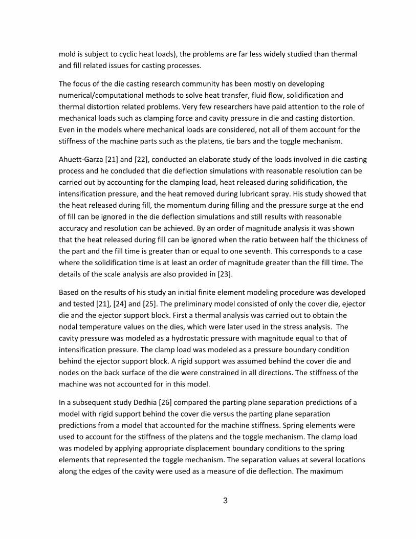
mold is subject to cyclic heat loads), the problems are far less widely studied than thermal
and fill related issues for casting processes.
The focus of the die casting research community has been mostly on developing
numerical/computational methods to solve heat transfer, fluid flow, solidification and
thermal distortion related problems. Very few researchers have paid attention to the role of
mechanical loads such as clamping force and cavity pressure in die and casting distortion.
Even in the models where mechanical loads are considered, not all of them account for the
stiffness of the machine parts such as the platens, tie bars and the toggle mechanism.
Ahuett‐Garza [21] and [22], conducted an elaborate study of the loads involved in die casting
process and he concluded that die deflection simulations with reasonable resolution can be
carried out by accounting for the clamping load, heat released during solidification, the
intensification pressure, and the heat removed during lubricant spray. His study showed that
the heat released during fill, the momentum during filling and the pressure surge at the end
of fill can be ignored in the die deflection simulations and still results with reasonable
accuracy and resolution can be achieved. By an order of magnitude analysis it was shown
that the heat released during fill can be ignored when the ratio between half the thickness of
the part and the fill time is greater than or equal to one seventh. This corresponds to a case
where the solidification time is at least an order of magnitude greater than the fill time. The
details of the scale analysis are also provided in [23].
Based on the results of his study an initial finite element modeling procedure was developed
and tested [21], [24] and [25]. The preliminary model consisted of only the cover die, ejector
die and the ejector support block. First a thermal analysis was carried out to obtain the
nodal temperature values on the dies, which were later used in the stress analysis. The
cavity pressure was modeled as a hydrostatic pressure with magnitude equal to that of
intensification pressure. The clamp load was modeled as a pressure boundary condition
behind the ejector support block. A rigid support was assumed behind the cover die and
nodes on the back surface of the die were constrained in all directions. The stiffness of the
machine was not accounted for in this model.
In a subsequent study Dedhia [26] compared the parting plane separation predictions of a
model with rigid support behind the cover die versus the parting plane separation
predictions from a model that accounted for the machine stiffness. Spring elements were
used to account for the stiffness of the platens and the toggle mechanism. The clamp load
was modeled by applying appropriate displacement boundary conditions to the spring
elements that represented the toggle mechanism. The separation values at several locations
along the edges of the cavity were used as a measure of die deflection. The maximum

4
separation value was about 12% to 20% higher in the model with spring elements than the
values from the model with rigid support, depending upon the design features of the die.
Choudhary [27] developed a finite element model in which the three machine platens, the C‐
frame and the tie bars were modeled explicitly. The die was a dummy structure that
consisted of two parallel plates connected by pillars on the four corners of the plates. A
roller support was modeled at the bottom of cover and ejector platens. A support block was
modeled at the bottom of the rear platen to prevent displacement in the vertical direction. A
small sliding contact was defined at all interfaces. The nodes on the either end of the tie bars
were tied to corresponding nodes on the ejector and rear platen. The clamp load was
applied as a pressure boundary condition on the toggle blocks on the cover and rear platens.
Thermal loads and cavity pressure were ignored in the model. The deflection of the cover
platen was predicted at eight different locations behind the cover platen and the results
were compared with corresponding values from the field data. The deflection pattern from
the simulations was similar to the pattern observed on the field data. But the individual
deflection values fell in the range of 10% to 15% of the observed field data. This model was
fairly accurate given the various approximations to the boundary conditions in the model
and the procedure followed to model the clamp load.
In another die distortion modeling study, Chayapathi [28] used a finite element model in
which the tie bars were explicitly modeled and the toggle mechanism was represented by
linear spring elements. The nodes on one end of the tie bar that are in contact with the
nodes in the cover platen were tied to the corresponding nodes on the cover platen. The
nodes on the other end of the tie bar were constrained in all six degrees of freedom. The
corner nodes on the bottom of the cover platen were constrained in vertical direction to
prevent rigid body motion. The clamp load was applied by specifying displacements on the
free end of the spring elements. The intensification pressure load was applied as a pressure
boundary condition on the cavity surfaces.
Ragab et al [29] experimentally verified the adequacy of this finite element model for
predicting the contact loads between the dies and platens on the cover and ejector sides.
The contact load between the platens and the dies were measured using a total of 35 load
cells, 18 load cells on the cover side and 17 load cells on the ejector side. The contact load
was measured under two different loading conditions, under clamp load only and during
actual casting operation. The load cells and the fixtures used in the experiments were also
explicitly included in the finite element model. The summation of cover side load cell
measurements decreased by 7% after intensification whereas the summation of cover side
load cell predictions from simulation remained constant. On the ejector side the summation
of load cell measurements and predictions remained constant. The difference between
5
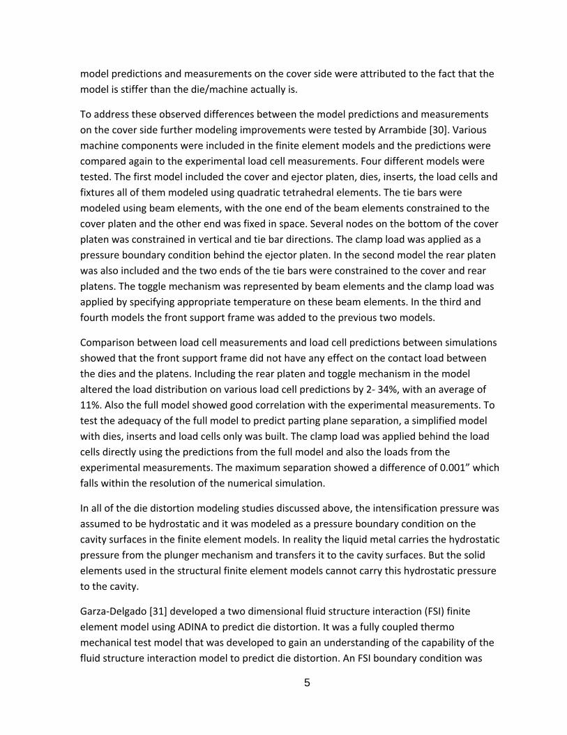
model predictions and measurements on the cover side were attributed to the fact that the
model is stiffer than the die/machine actually is.
To address these observed differences between the model predictions and measurements
on the cover side further modeling improvements were tested by Arrambide [30]. Various
machine components were included in the finite element models and the predictions were
compared again to the experimental load cell measurements. Four different models were
tested. The first model included the cover and ejector platen, dies, inserts, the load cells and
fixtures all of them modeled using quadratic tetrahedral elements. The tie bars were
modeled using beam elements, with the one end of the beam elements constrained to the
cover platen and the other end was fixed in space. Several nodes on the bottom of the cover
platen was constrained in vertical and tie bar directions. The clamp load was applied as a
pressure boundary condition behind the ejector platen. In the second model the rear platen
was also included and the two ends of the tie bars were constrained to the cover and rear
platens. The toggle mechanism was represented by beam elements and the clamp load was
applied by specifying appropriate temperature on these beam elements. In the third and
fourth models the front support frame was added to the previous two models.
Comparison between load cell measurements and load cell predictions between simulations
showed that the front support frame did not have any effect on the contact load between
the dies and the platens. Including the rear platen and toggle mechanism in the model
altered the load distribution on various load cell predictions by 2‐ 34%, with an average of
11%. Also the full model showed good correlation with the experimental measurements. To
test the adequacy of the full model to predict parting plane separation, a simplified model
with dies, inserts and load cells only was built. The clamp load was applied behind the load
cells directly using the predictions from the full model and also the loads from the
experimental measurements. The maximum separation showed a difference of 0.001” which
falls within the resolution of the numerical simulation.
In all of the die distortion modeling studies discussed above, the intensification pressure was
assumed to be hydrostatic and it was modeled as a pressure boundary condition on the
cavity surfaces in the finite element models. In reality the liquid metal carries the hydrostatic
pressure from the plunger mechanism and transfers it to the cavity surfaces. But the solid
elements used in the structural finite element models cannot carry this hydrostatic pressure
to the cavity.
Garza‐Delgado [31] developed a two dimensional fluid structure interaction (FSI) finite
element model using ADINA to predict die distortion. It was a fully coupled thermo
mechanical test model that was developed to gain an understanding of the capability of the
fluid structure interaction model to predict die distortion. An FSI boundary condition was
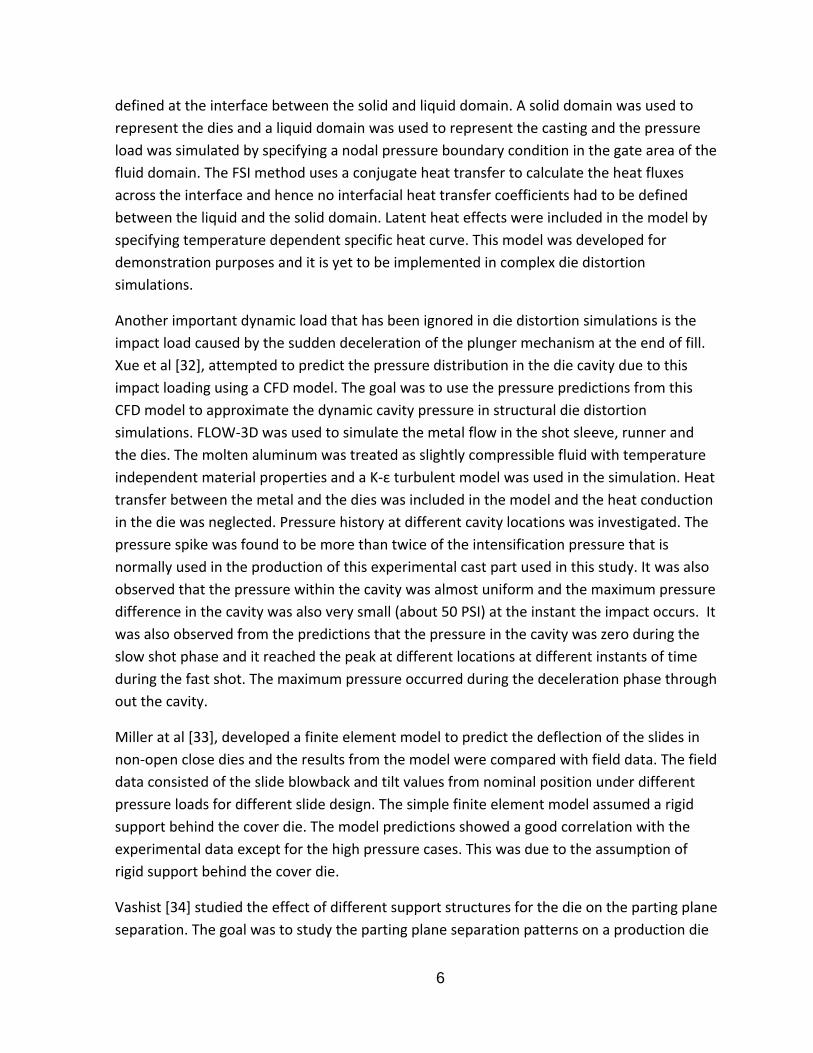
6
defined at the interface between the solid and liquid domain. A solid domain was used to
represent the dies and a liquid domain was used to represent the casting and the pressure
load was simulated by specifying a nodal pressure boundary condition in the gate area of the
fluid domain. The FSI method uses a conjugate heat transfer to calculate the heat fluxes
across the interface and hence no interfacial heat transfer coefficients had to be defined
between the liquid and the solid domain. Latent heat effects were included in the model by
specifying temperature dependent specific heat curve. This model was developed for
demonstration purposes and it is yet to be implemented in complex die distortion
simulations.
Another important dynamic load that has been ignored in die distortion simulations is the
impact load caused by the sudden deceleration of the plunger mechanism at the end of fill.
Xue et al [32], attempted to predict the pressure distribution in the die cavity due to this
impact loading using a CFD model. The goal was to use the pressure predictions from this
CFD model to approximate the dynamic cavity pressure in structural die distortion
simulations. FLOW‐3D was used to simulate the metal flow in the shot sleeve, runner and
the dies. The molten aluminum was treated as slightly compressible fluid with temperature
independent material properties and a K‐ε turbulent model was used in the simulation. Heat
transfer between the metal and the dies was included in the model and the heat conduction
in the die was neglected. Pressure history at different cavity locations was investigated. The
pressure spike was found to be more than twice of the intensification pressure that is
normally used in the production of this experimental cast part used in this study. It was also
observed that the pressure within the cavity was almost uniform and the maximum pressure
difference in the cavity was also very small (about 50 PSI) at the instant the impact occurs. It
was also observed from the predictions that the pressure in the cavity was zero during the
slow shot phase and it reached the peak at different locations at different instants of time
during the fast shot. The maximum pressure occurred during the deceleration phase through
out the cavity.
Miller at al [33], developed a finite element model to predict the deflection of the slides in
non‐open close dies and the results from the model were compared with field data. The field
data consisted of the slide blowback and tilt values from nominal position under different
pressure loads for different slide design. The simple finite element model assumed a rigid
support behind the cover die. The model predictions showed a good correlation with the
experimental data except for the high pressure cases. This was due to the assumption of
rigid support behind the cover die.
Vashist [34] studied the effect of different support structures for the die on the parting plane
separation. The goal was to study the parting plane separation patterns on a production die

7
that flashed severely after it was moved from a 1000 ton machine to a 2500 ton machine.
The die had to be mounted lower on the 2500 ton machine due to the location of the shot
hole. Therefore, to evenly spread out the clamp load, the die foot print was increased on the
cover on the machine platen by adding support structures to the dies. This study analyzed
the effect of different types of support structures and different clamp loads. The results
showed that the added supports stiffened the die/machine structure and increased the
platen coverage area, but they did not aid in transferring the clamp load to the die faces.
Flynn et al [35] measured the deflection of the same production die at various locations of
the die using LVDT’s and they reported a good match between the model predictions by
Vashist [34] and the experimental measurements.
Garza‐Delgado [36] studied the failure of tie bolts that occurred on a hot chamber machine,
using a sequentially coupled thermo mechanical model. This case study showed that non‐
uniform heat growth on the parting surface of the die resulted in unequal distribution of
loads on the tie bolts and resulted in tie bolts failure. The machine frame, shank and bracket
were modeled explicitly in the structural model. The toggle mechanism and the tie bolts
were modeled using 3D beam elements.
Barone and Caulk [39] presented a method to predict the ultimate distortion of both the
casting and the die due to thermal and mechanical loads in the die casting process. They
formulated the die distortion problem as a nonlinear thermo elastic contact problem solved
by iterative boundary element method. But the casting distortion was analyzed as an
unconstrained thermo elastic shrinkage using finite element method. Their model included
the dies, the ejector support, and cover and ejector platens. The tie bars and toggle
mechanisms were represented by spring elements behind the ejector and cover platen
respectively with appropriate stiffness values. Suitable displacement constraints were
provided on selected nodes on the bottom of the cover platen to prevent rigid body motion
of the entire structure. This boundary condition is an approximation of anchoring the
machine to the base. The uneven contact on the parting surface was handled using
contact/gap elements whose formulation provides for load transfer between the die
components only when the mutual surface traction is compressive. Friction between the
contact surfaces were ignored in this model. The cavity pressure was modeled as a
hydrostatic pressure with a magnitude equal to that of the intensification pressure. The
modeling approach was tested on a front drive transmission case die and the results were
presented. The advantage of this method as claimed by the authors is that the casting and
die distortion can be analyzed simultaneously and the shrinkage allowance for the die cavity
can be estimated.

8
Ragab et al [40] studied the effect of casting material constitutive model on the deflection
and residual stress predictions on the casting. The cover and ejector platens were included in
the model and the tie bars were represented using spring elements. The clamp load was
applied by specifying displacement boundary condition on the spring elements representing
the toggle mechanism. The cavity pressure was modeled as a pressure boundary condition.
A contact constraint was used between the die and the casting. A fully coupled thermo
mechanical analysis was conducted. Three different material models were considered for the
casting, viz., elastic, elastic‐plastic and elastic‐viscoplastic. The residual stress predictions
were affected significantly by the material models. The distortion predictions were less
affected. The elastic model overestimated the stresses and the visco‐plastic model lacked
the required material property data. Therefore in a further study Ragab, [41] used the
elastic‐plastic model to predict the effect of key modeling factors on casting distortion
predictions. The factors considered were the yield strength and strain hardening of the
casting material, the heat transfer coefficient between the die and the casting and the
injection temperature of the metal. The study concluded that the yield strength had a major
effect on residual stresses at ejection while the injection temperature and the heat transfer
coefficient had a major effect on the residual stresses at room temperature. The
disadvantage of the model used in Ragab’s study was that the solid casting could not follow
the distorted shape of the cavity due to the use of solid elements for the castings and hence
it might affect the casting distortion prediction.
Garza‐Delgado [42] addressed this issue by using a shell mesh representing the casting
surface in the sequentially coupled thermo mechanical model that included the clamp loads,
intensification pressure load and the thermal load. The nodal distortion values of the shell
mesh were then mapped on to the surface nodes of a solid mesh for the casting. Then the
solid cavity was tied to the distorted shape of the die using tied contact and the cooling
stages of the casting were simulated using a fully coupled elastic‐plastic thermo mechanical
model. Modeling the tie bars explicitly and applying the clamp loads through spring
elements caused problems in establishing contact between the die and the casting.
Therefore the clamp force was modeled as a pressure boundary condition behind the ejector
platen in this work.
Numerous parametric die design studies has been conducted at the Center for Die Casting at
Ohio State University to understand the role of structural die design parameters on die
deflection. Some of these parametric die design studies are reviewed here.
Jayaraman [43], conducted a parametric study of the slide design variables for an inboard
lock design and the work was continued by Chakravarti [44, 45] using a refined model. The
variables considered were the preload, the angle of the locking surface and the pivot. Results

9
suggested that the preload had no effect on the blowback and tilt values but it affected the
fatigue life of the slides. The trends also showed that the tip separation increased with
locking face angle and slides with high pivot were better supported by the ejector platen.
There was negligible effect on the parting plane separation within the range of design
variables.
The effect of proud inserts on the parting plane separation was first analyzed by Dedhia [26],
[46]. The study concluded that using proud inserts resulted in a lower separation during the
initial cycles but at the later stages as the die warms up and grows the separation values
were similar to the cases with flush inserts (insert parting surface in line with the die parting
surface). A much refined model was later used by Tewari [3], [45] to study the effect of
proud inserts on the parting plane separation. The contact pressure between the dies and
the platens and the compressive stresses in the die pocket were also studied. It was
observed that the parting plane separation was reduced around the cavity by having a proud
insert and the contact pressure between the dies and the platens was not affected due to
the use of proud inserts. The proud insert had negligible effect on the compressive stresses
in the die pocket.
Tewari [3], [45], analyzed the effect of adding a back plate behind the ejector support box.
Results from his study indicate that the back plate has negligible effect on both the parting
plane separation and the contact pressure between the ejector die and the platen.
A parametric study conducted by Dedhia et al [26], [46], showed that using proud pillars had
no effect on the parting plane separation. The difference in parting plane separation values
between the cases with proud pillars and flush pillars was less than 5%.
A series of parametric studies [1‐3], [28] were conducted to gain understanding of the effect
of important structural variables of the dies and the machine on the die distortion. The
summary of the work was published in [4], [45].
The variables investigated were die size (% of platen area covered), insert thickness,
thickness of die steel behind the insert and die location on the platen. Response surface
models based on design of experiments were used to study the interaction between the
variables and their effect of parting plane separation. The approach for the sensitivity
analysis was developed by Chayapathi [1], [28] and the initial experimental design array
consisted of 15 experimental runs. An additional 16 runs were further added by Kulkarni
and Tewari [2], [3] to ascertain the results. The study has shown that the dominant factor
that affects the die distortion on the cover side is the cover platen thickness. Thin dies
performed better than thick dies. The more the steel behind the dies the lesser was the
parting plane separation observed. Small or medium sized dies (covering 40% to 50% of

10
platen area) performed better. Kulkarni [2] attempted to study the cover and ejector side
performances separately. But the ejector side design variables such as the rail size, number,
size and location of the support pillars were not controlled in the computational
experiments. Therefore the study was inconclusive about the contribution of ejector side
design to the ejector side separation.
2.2 SummaryoftheState‐of‐the‐ArtThe state‐of‐the‐art in modeling the die casting die/machine system is briefly summarized in
this section to place the work performed in this project in context.
The vast majority of die casting modeling work performed in industry addresses flow
modeling of die filling and thermal modeling of the part and die as the die cools. In virtually
every case the machine is ignored except as the source of the metal speed during filling and
the die is assumed to be completely rigid except possibly for thermal growth. There is
generally no consideration of the mechanical forces and pressures at work in the system.
As described in the previous section, the work at Ohio State over the past several years has
addressed and developed structural modeling techniques and boundary conditions suitable
to model many aspects of the system response to the machine clamping forces, cavity and
injection pressure, as well as the thermal loads that most modeling considers. A depiction of
the major components of the system as typically modeled is shown in Figure 1.
Figure 1 Typical Die Casting System Model Used by OSU

11
The machine base, all three platens (assuming a three platen system), the cover and ejector
die components, and the tie bars are explicitly modeled. The machine clamping mechanism
is represented with beam elements whose length is adjusted to provide the proper clamp
magnitude.
The part and die cavity are typically modeled independently and the system is analyzed in
quasi steady state by modeling 50 or more thermal cycles of the die so that the time‐varying
die temperature field is consistent from one cycle to the next. The structural analysis is
static and the cavity pressure is not explicitly modeled but addressed with a hydrostatic
boundary condition. The inability to explicitly model the pressure at the interface between
the casting and the die is one of the limiting factors in developing robust models of part
distortion. Overall, the modeling approach has proven to be quite robust and useful but it
does require considerable understanding of the mechanics of the system and of structural
modeling. Consequently, structural modeling of the system is not yet widely practiced in
industry as a design tool. It is, however, beginning to be used for trouble shooting system
failures.
2.3 ObjectivesIn general terms, the objectives of this project are to make the principles and methods of
system structural modeling more accessible to the industry through the development of
detailed tutorial material and through the use of meta‐models (models of models) that
capture the results of simulations in relatively simple dimensionless equations that can be
programmed on a spread sheet or in a simple computer application. In addition, the issue of
the pressure boundary condition mentioned above is explored in some detail and areas of
the modeling that are less well developed, specifically the design of the ejector side of the
die, are explored.
Several of the industrial case studies summarized in the previous section show that even
very experienced process engineers and tooling designers often incorrectly predict how the
die will respond to changes to the structural elements in the die assembly. Industry does not
always apply basic engineering principles when considering die mechanical performance. As
a consequence considerable time and money is spent trying out die design options that
ultimately do not work. This process results in very long try outs with many scrapped
castings. These problems can be avoided or at least minimized with corresponding savings of
wasted energy.
Specific goals included:
Systematically addressing design of the ejector side of the die casting die.
Develop parametric information about the relationship between die shoe design,
slide carrier design, and the machine.

12
Analyzing the relationship between the die center of pressure, die geometric center,
and platen center of pressure in the pursuit of better setup guidelines.
Examine the possibility of explicitly modeling the casting/die interface with the
objective of eliminating the need to use a pressure boundary condition
Provide design guidelines for the industry addressing the mechanical design of dies
and the relationship between die and machine.
2.4 TasksandApproachThe tasks to meet these goals include:
1. Analysis of Die Position Effects
Approach – A collection of computational experiments designed using design of
experiments principles was used to develop FEA models of dies in various configurations
on the die casting machine. Then through the application of dimensional analysis, the
data produced along with data from other experiments performed by the group, were
then used to construct a dimensionless power law model to predicting tie bar balance as
a function of die configuration parameters. This task is closely related to task 4
described below.
2. Die Failure Case Study
Approach – A study was performed in conjunction with an industry partner that analyzed
the root cause of premature cracking of a die used to produce a door closer housing.
The crack resulted in a surface blemish that resulted in castings being rejected. The
primary purpose of this task was to gain more modeling experience with failures and to
extend the modeling procedures to consider these issues.
3. Cavity Pressure Modeling Methods
Approach – A comprehensive FEA modeling study supported with results from casting
experiments and a separate set of experiments to obtain high temperature stress‐strain
properties was used.
4. Evaluation of Ejector Side and Slide Design
Approach ‐ A collection of computational experiments designed using design of
experiments principles was used to develop FEA models of various die shoe and pillar
configurations. Then through the application of dimensional analysis, the were used to
construct a dimensionless power law model to predicting maximum parting plane
separation as a function of design parameters. This task is closely related to task 1
described above.
5. Modeling and Design Guidelines

13
Approach – Drawing on experiences with modeling performed as part of this project and
with the previous work summarized in the previous section, a comprehensive modeling
tutorial was developed. In addition, a very short summary of key principles was
developed as an introduction to the area.
14
3. ResultsandDiscussion
3.1 AnalysisofDiePositionEffectsA brief description of the modeling and analysis performed for this task is presented below.
A summary report that describes the die position analysis work is presented in Appendix A.
This report was provided to NADCA for distribution to the industry and also contains the
summary for the ejector side design work.
A simplified representation of a die casting machine and die used for modeling was shown in
Figure 1 previously.
The die is clamped and held closed by the combination of a toggle mechanism (represented
as beam elements in the figure) and tie bars that are anchored to the cover and rear platen.
The ejector platen moves with the toggle to open the die. The tie bars act much like bolts or
a clamp in providing the restraining force needed to keep the die closed. The degree to
which the die is held closed and pressure on the parting surfaces of the die are relatively
uniform depends on the thermal growth of the die, the cavity shape and the placement of
the position of the die on the platens.
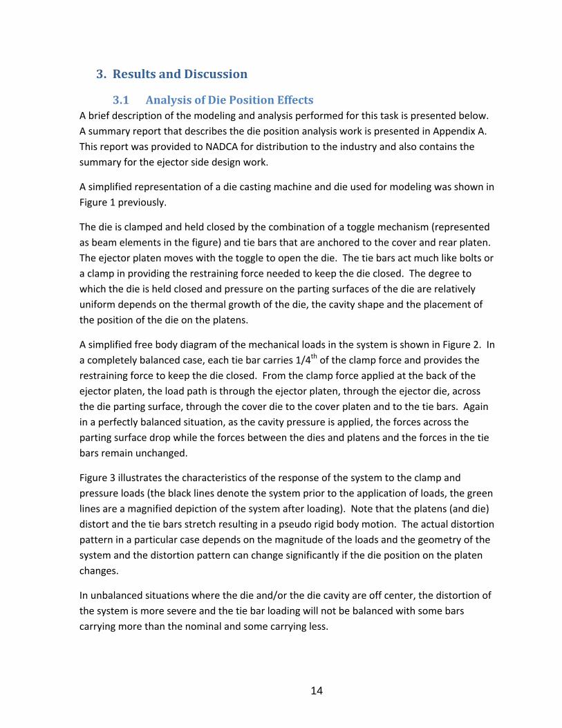
A simplified free body diagram of the mechanical loads in the system is shown in Figure 2. In
a completely balanced case, each tie bar carries 1/4th of the clamp force and provides the
restraining force to keep the die closed. From the clamp force applied at the back of the
ejector platen, the load path is through the ejector platen, through the ejector die, across
the die parting surface, through the cover die to the cover platen and to the tie bars. Again
in a perfectly balanced situation, as the cavity pressure is applied, the forces across the
parting surface drop while the forces between the dies and platens and the forces in the tie
bars remain unchanged.
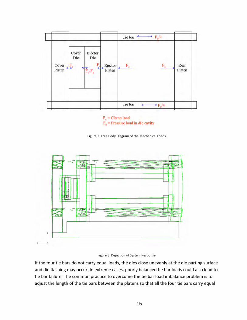
Figure 3 illustrates the characteristics of the response of the system to the clamp and
pressure loads (the black lines denote the system prior to the application of loads, the green
lines are a magnified depiction of the system after loading). Note that the platens (and die)
distort and the tie bars stretch resulting in a pseudo rigid body motion. The actual distortion
pattern in a particular case depends on the magnitude of the loads and the geometry of the
system and the distortion pattern can change significantly if the die position on the platen
changes.
In unbalanced situations where the die and/or the die cavity are off center, the distortion of
the system is more severe and the tie bar loading will not be balanced with some bars
carrying more than the nominal and some carrying less.
15
Figure 2 Free Body Diagram of the Mechanical Loads
Figure 3 Depiction of System Response
If the four tie bars do not carry equal loads, the dies close unevenly at the die parting surface
and die flashing may occur. In extreme cases, poorly balanced tie bar loads could also lead to
tie bar failure. The common practice to overcome the tie bar load imbalance problem is to
adjust the length of the tie bars between the platens so that all the four tie bars carry equal

16
loads. In such a case the minimum clamp load required to hold the dies together will be
higher than the one that would be needed if the dies were centered on the platen thus
limiting the capacity of the machine.
The current approach used in industry to predict the tie bar loads balances the moments due
to the cavity pressure but ignores the location of the die with respect to the platen center
and it assumes that the machine and the dies are perfectly rigid and consequently can be
quite inaccurate.
To address these issues, a non‐linear power law model was developed to predict the tie bar
loads of the die casting machine based on the location of the die and cavity center of
pressure with respect to the tie bars. The model was obtained by curve fit to tie bar load
prediction data from computational experiments. The computational experiments were
conducted using the finite element modeling. An experimental design was developed based
on the horizontal and vertical dimension of the die, the locations of the die and cavity center
of pressure with respect to the platen center and the magnitude of cavity center of pressure.
Dimensional analysis was used to incorporate other important scale factors and obtain the
non‐dimensional parameters. The non‐linear model was then fit to the non‐dimensional
form of the location, scale and load variables. Experimental tie bar load measurements were
then compared to the power law model predictions to check the adequacy of the power law
models.
3.1.1 ComputationalExperimentsThe factors that were considered are the die length, die width, location of the die with
respect to the platen center and the location of the cavity center of pressure with respect to
the platen center and the magnitude of the cavity pressure. The description of the variables
and their levels are shown in Table 1. The location variables are defined with respect to a
coordinate system with origin on the center of the platen area between the tie bars. The
schematic of the coordinate system and the tie bar labels are shown in Figure 4 .

17
Factor Factor Description Level
1
Level
2
Level
3
Level
4
Level
5
LX Die Width (inches) 26.49 30.4 32.6 34.6 36.5
LY Die Height (inches) 26.49 30.4 32.6 34.6 36.5
DPX Die location in X‐
direction (inches) ‐4 ‐2 0 2 4
DPY Die location in Y‐
direction (inches) ‐4 ‐2 0 2 4
CPX
Location of center of
pressure in X‐
direction (inches)
‐4 ‐2 0 2 4
CPY
Location of center of
pressure in Y‐direction
(inches)
‐4 ‐2 0 2 4
CPR Cavity Pressure (KSI) 2 4 6 8 1
Table 1 Description of Variables
Figure 4 Coordinate System and Tie bar Labels
A few additional cases were also added to the experimental array to include cases with a
cavity load equal to 100% of clamp load and a few cases with no cavity pressure load.
3.1.2 DimensionalAnalysisDimensional analysis and an analysis of the physical phenomena involved lead to a power
law form shown in (1)

18
c1 c2
tb tb
t b tb
Tie bar load DPX DPY=c0 1± 1+ ×
Nominal Load 0.5L 0.5L
CPR×A CPX CPY CPR×A× 1+c3 exp 1± +c4 1+ ×
CLAMP 0.5L 0.5L CLAMP
CPR×A CPR×A× 1-c5 ×exp
CLAMP
CLAMP
(1)
This form was assumed for each individual tie bar and parameters selected to fit the power
law to the predicted loads for each of the four tie bars for all of the 70 cases in the
experimental array. The SPSS statistical software package was used to perform the non‐
linear regression and the sequential quadratic programming algorithm in SPSS was used to
solve the non‐linear regression problem.
The same model form was obtained for all the four tie bars and the magnitudes of the
coefficients and exponents for the two top tie bars were approximately equal with different
signs. Similarly the magnitudes of the exponents and coefficients for the two bottom tie bars
were nearly the same. Therefore the load data for the top tie bars were pooled and the data
for the bottom tie bars were pooled and the same model form was fit to the pooled data.
The results are given by equations (2) and (3) respectively. The terms with +/‐ signs are
reversed between the two equations. These parameters represent the vertical location of
the die and center of pressure respectively and hence their signs are positive for the top tie
bars and negative for the bottom tie bars.
The parameter estimates, the standard error in the estimates and the confidence intervals
for the estimates for the top and bottom tie bars are provided in Table 2and Table 3
respectively. The quality of the fit is clearly very good.
The resulting equations are as follows:
0.354 0.303
tb tb
tb tb
Top Tie bar load DPX DPY=1.005 1± 1+ ×
Nominal Load 0.5L 0.5L
CPR×A CPX CPY CPR×A× 1+0.063 exp 1± +0.886 1+ ×
CLAMP 0.5L 0.5L CLAMP
× 1-0.
CPR×A CPR×A098 ×exp
CLAMP CLAMP
(2)

19
0.294 0.256
tb t b
tb t b
Bottom Tie bar load DPX DPY=1.04 1± 1- ×
Nominal Load 0.5L 0.5L
CPR×A CPX CPY CPR×A× 1+0.062 exp 1± +1.03 1- ×
CLAMP 0.5L 0.5L CLAMP
× 1-0
CPR×A CPR×A.106 ×exp
CLAMP CLAMP
(3)
Parameter Estimates
Parameter Estimate
Std.
Error
95% Confidence
Interval
Lower
Bound
Upper
Bound
c0 1.005 0.002 1.001 1.009
c1 0.354 0.011 0.333 0.374
c2 0.303 0.012 0.279 0.327
c3 0.063 0.005 0.052 0.074
c4 0.886 0.045 0.796 0.976
c5 ‐0.098 0.006 ‐0.109 ‐0.086
Adjusted R‐square = 0.96
Table 2: Parameter Estimates for Top Tie Bar Model Fit
20
Parameter Estimates
Parameter Estimate
Std.
Error
95% Confidence
Interval
Lower
Bound
Upper
Bound
c0 1.04 0.002 1.036 1.044
c1 0.294 0.012 0.271 0.318
c2 0.256 0.014 0.228 0.284
c3 0.062 0.005 0.051 0.073
c4 1.025 0.052 0.922 1.128
c5 ‐0.106 0.005 ‐0.117 ‐0.095
Adjusted R‐Square = 0.95
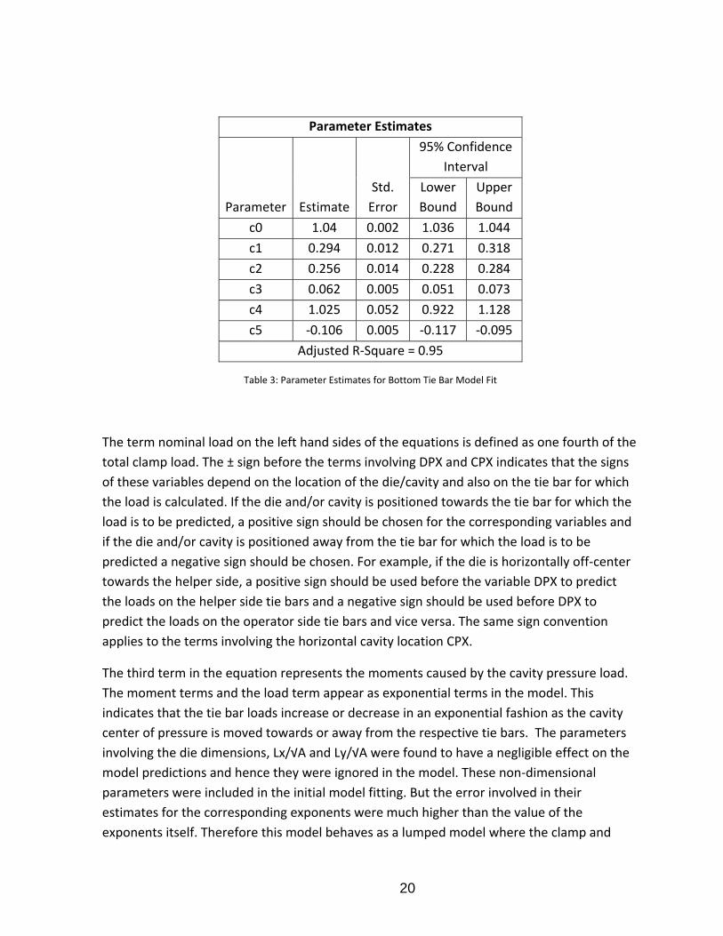
Table 3: Parameter Estimates for Bottom Tie Bar Model Fit
The term nominal load on the left hand sides of the equations is defined as one fourth of the
total clamp load. The ± sign before the terms involving DPX and CPX indicates that the signs
of these variables depend on the location of the die/cavity and also on the tie bar for which
the load is calculated. If the die and/or cavity is positioned towards the tie bar for which the
load is to be predicted, a positive sign should be chosen for the corresponding variables and
if the die and/or cavity is positioned away from the tie bar for which the load is to be
predicted a negative sign should be chosen. For example, if the die is horizontally off‐center
towards the helper side, a positive sign should be used before the variable DPX to predict
the loads on the helper side tie bars and a negative sign should be used before DPX to
predict the loads on the operator side tie bars and vice versa. The same sign convention
applies to the terms involving the horizontal cavity location CPX.
The third term in the equation represents the moments caused by the cavity pressure load.
The moment terms and the load term appear as exponential terms in the model. This
indicates that the tie bar loads increase or decrease in an exponential fashion as the cavity
center of pressure is moved towards or away from the respective tie bars. The parameters
involving the die dimensions, Lx/√A and Ly/√A were found to have a negligible effect on the
model predictions and hence they were ignored in the model. These non‐dimensional
parameters were included in the initial model fitting. But the error involved in their
estimates for the corresponding exponents were much higher than the value of the
exponents itself. Therefore this model behaves as a lumped model where the clamp and

21
pressure loads are approximated by point loads acting on the die center and cavity center of
pressure respectively.
3.1.3 ModelAdequacy,FEAResultsThe power law models shown in equations (2) and (3) were obtained by curve fitting to tie
data from a 800 ton four toggle machine. To study the adequacy of the model to predict the
tie bar loads on machines of other designs and clamping capacity, the power law model
predictions were compared against the finite element model predictions of tie bar load on
machines of other designs and tonnages. Three different machine finite element models
were considered, viz, a 3500 ton four toggle machine, 1000 ton four toggle machine and a
250 ton two toggle machines. The die location, cavity location, the clamp load and
magnitude of cavity pressure for these three cases are summarized in Table 4. The FEA and
power law predictions, presented as the difference from nominal, for the same four cases
are shown in Table 5, Table 6, and Table 7 respectively.
Machine
Design
DPX
(in)
DPY
(in)
CPX
(in)
CPY
(in)
CPR
(PSI)
Ltb
(in)
Cavity
Load
(tons)
Clamp
Load
(tons)
3500 ton‐4
toggle 4 0 4 0 0 84.25 0 3500
1000‐ton‐
4 toggle 0 1.25 0 3.63 10000 44 602 722
250‐ton‐2
toggle 0 ‐3.14 0 ‐0.423 10000 21.75 135 250
Table 4: Summary of Finite Element Models
Tie Bar Load/Nominal Load Prediction
FEA Power Law
Top Tie Bar‐1 ‐3.8% ‐3.0%
Top Tie Bar‐2 2.8% 3.8%
Bottom Tie Bar‐1 ‐2.9% ‐2.6%
Bottom Tie Bar‐2 4.0% 3.1%
Table 5: Comparison of Model Predictions for a 3500 Ton Machine
(DPX=4”, DPY=0”, CPX=4”, CPY=0”, CPR=0 PSI)

22
Tie Bar Load/Nominal Load Prediction
FEA Power Law
Top Tie Bar‐1 4.1% 6.7%
Top Tie Bar‐2 4.1% 6.7%
Bottom Tie Bar‐1 ‐4.1% ‐2.1%
Bottom Tie Bar‐2 ‐4.1% ‐2.1%
Table 6: Comparison of Model Predictions for a 1000 Ton Machine
(DPX=0”, DPY=1.25”, CPX=0”, CPY=3.63”, CPR=10000 PSI)
Tie Bar Load/Nominal Load Prediction
FEA Power Law
Top Tie Bar‐1 ‐8.2% ‐8.3%
Top Tie Bar‐2 ‐8.2% ‐8.3%
Bottom Tie Bar‐1 8.2% 14%
Bottom Tie Bar‐2 8.2% 14%
Table 7: Comparison of Model Predictions for a 250 Ton Machine
(DPX=0”, DPY=‐3.14”, CPX=0”, CPY=‐0.423”, CPR=10000 PSI)
The 1000 and 250 ton machines have very different designs compared to the 800 and 3500
ton machines and the FEA analyses in these cases used simplified boundary conditions on
the cover platen. The difference in boundary conditions, and not the difference in design, is
largely responsible for the constant magnitude FEA results in the two cases in question.
The results show reasonably good predictive capability across a variety of designs as
expected of a dimensionless model.
3.1.4ModelAdequacy,ExperimentalMeasurementsExperiments were conducted on a 250 ton two‐toggle machine by varying the die location
and obtaining the tie bar loads under clamp load only. The schematic of the test die on the
machine platens is shown in Figure 5. The test die measures 13.38 inches by 18 inches and
the distance between the tie bar centers is 21.75 inches. Four uniaxial strain gauges were
attached to each tie bar to measure the longitudinal strains. The strain gauges were
attached to the tie bars at a distance of 267 mm (10.5 in) from the inside face of the
stationary platen so that the strain gauges are half‐way between the stationary and movable
platens when the test die is closed. The schematic of the strain gauge locations is shown in

23
Figure 6. The four strain gauges on each tie bar are 90ο apart. Thirteen different die setups
were studied, one with a die centered on the platen, four cases with vertically off center
dies, four cases with horizontally off center dies and four cases with diagonally off center
dies. The thirteen cases are summarized in Table 8 . Not all combinations of diagonally off
center dies could be studied due to the limitation of the space available between the tie
bars.
Figure 5 Schematic of the test die on the machine platens
Figure 6 Schematic of strain gauges and coordinate system

24
Run DPX
(inches) DPY (inches)
1 0 0
2 0 2
3 0 4
4 2 0
5 4 0
6 0 ‐2
7 0 ‐4
8 ‐2 0
9 ‐4 0
10 2 1.875
11 4 1.875
12 ‐2 ‐1.875
13 ‐4 ‐1.875
Table 8: Experimental Array
Each case was repeated three times and a constant clamp load of 2500 KN was applied in all
cases. Though the machine was programmed to apply a clamping load of 2500 KN, the actual
clamp load applied by the machine varies slightly from the nominal. The metal injection
stage was ignored in these experiments due to the practical difficulty of moving the shot
sleeve for each test. The strains on each tie bar were obtained under clamp load only. The
average of the strains measured by the four strain gauges on each tie bar was calculated to
obtain the strain on each tie bar. The tie bar loads were then calculated from the strain
values. The nominal clamp load per tie bar was assumed to be the average of the four tie bar
loads and the load on each tie bar was estimated as the ratio between the tie bar load and
the nominal load.
The experimental measurements and power law predictions of tie bar loads for the thirteen
cases are shown in Table 9 and Figure 7. Ideally the loads on all four tie bars should be equal
for case‐1 where the dies are centered on the platen. However the measurements show that
the loads on bottom tie bars are lower than on the top tie bars. This could be due to
inaccuracy in positioning the dies on the platen causing the measurements to be biased
towards the top tie bars. Lack of squareness and perfect flatness of the platens could also
contribute to this observed difference.

25
Case DPX DPY
Experimental
Measurements Power Law Predictions
T1 T2 B1 B2 T1 T2 B1 B2
1 0 0 1.03 1.02 0.99 0.97 1.00 1.01 1.04 1.04
2 0 2 1.10 1.09 0.92 0.90 1.05 1.06 0.99 0.99
3 0 4 1.16 1.15 0.85 0.83 1.10 1.11 0.93 0.93
4 2 0 0.99 1.09 0.90 1.02 0.94 1.07 0.98 1.09
5 4 0 0.94 1.14 0.85 1.07 0.86 1.12 0.91 1.13
6 0 ‐2 0.96 0.95 1.05 1.04 0.94 0.95 1.08 1.08
7 0 ‐4 0.92 0.90 1.10 1.08 0.87 0.88 1.12 1.12
8 ‐2 0 1.09 0.98 1.03 0.91 1.06 0.94 1.09 0.98
9 ‐4 0 1.16 0.92 1.09 0.83 1.11 0.86 1.13 0.92
10 2 1.875 1.06 1.15 0.84 0.95 0.98 1.12 0.93 1.04
11 4 1.875 1.03 1.22 0.76 1.00 0.90 1.17 0.87 1.08
12 ‐2 ‐1.875 1.02 0.90 1.11 0.97 1.00 0.89 1.13 1.02
13 ‐4 ‐1.875 1.08 0.84 1.17 0.91 1.05 0.82 1.18 0.95
Table 9: Comparison of Measurements and Predictions
The data show that the model predictions are consistently slightly lower than the
experimental measurements for the top tie bars and they are consistently slightly higher
than the measurements for the bottom tie bars in all of the 13 cases. This can be attributed
to the constraint type used between the cover platen and the machine base for the FEA
model used to construct the meta‐model. The edge nodes of the cover platen and the base
were tied using a multi‐point constraint in the computational (FEA) experiments that created
the data for the meta‐model. Though the 250‐ton machine used for the experiments has a
welded joint the multi‐point constraint used in the FEA might be stiffer than the actual
welded joint on the machine. The lack of flatness and squareness of the dies could also have
contributed to some of these differences.

26
Figure 7 Tie bar Load Measurements vs. Predictions
The differences between the measurements and model predictions are shown in Table 10.
The differences between the model predictions and the load measurements vary from 0.1%
to 12% depending on the die location. As expected, the worst cases are the diagonally off
center cases, case‐10 and case‐11, where the measurements show that the load on the top
tie bar‐1 (T1) is higher than the nominal and the model predictions show that the loads on
top tie bar‐1 (T1) is lower than the nominal. Similarly the load measurements on bottom tie
bar‐1 (B2) are lower than the nominal in case‐10 and case‐11, and the model predictions
show that they are higher than the nominal. Overall, the pattern of results is very good.
Note again that the power law was derived from simulation data based on an 800 ton, 4
toggle machine and the experimental data is from a 250 ton, 2 toggle machine adding
credibility to the claim that the power law produces reasonable predictions for a wide
variety of machine designs and sizes.

27
Case DPX DPY
Difference between Measurements and Model
Predictions (%)
T1 T2 B1 B2
1 0 0 2.54% 1.26% ‐4.83% ‐7.40%
2 0 2 4.50% 2.84% ‐6.77% ‐9.17%
3 0 4 6.52% 4.59% ‐7.20% ‐9.76%
4 2 0 5.40% 2.03% ‐7.72% ‐6.95%
5 4 0 7.63% 2.24% ‐6.75% ‐6.03%
6 0 ‐2 1.98% 0.10% ‐2.75% ‐4.90%
7 0 ‐4 4.28% 2.13% ‐1.80% ‐4.32%
8 ‐2 0 2.80% 3.37% ‐5.10% ‐7.81%
9 ‐4 0 5.19% 5.90% ‐3.89% ‐9.10%
10 2 1.875 8.15% 3.25% ‐9.65% ‐9.23%
11 4 1.875 12.33% 4.66% ‐11.54% ‐8.60%
12 ‐2 ‐1.875 2.49% 1.02% ‐2.25% ‐5.41%
13 ‐4 ‐1.875 3.39% 2.29% ‐0.91% ‐4.14%
Table 10: Difference between Measurements and Model Predictions
3.2 DieFailureCaseStudyThe die used to produce the housing of a door closing mechanism suffered premature cracks
on the ejector die cavity surface. These cracks led to visible marks on the casting surface
making the casting unacceptable. The onset of the cracks in the ejector die occurred at
approximately 20,000 – 40,000 shots, much below the design expectation leading to
unexpected cost elevation. Several techniques were tried by the die caster to fix the
problem, but with no success. Since the cause of the problem was thought to be flexing of
the die, the Center for Die Casting at Ohio State University was asked to analyze the die
using die distortion modeling techniques developed over the past several years. The
problem was expected to provide a good case study for testing the analysis procedures.
Figure 8 and Figure 9 illustrate the casting and the surface defect. Several modifications
were made to the casting and the ejector insert to avoid the crack formation with little
success. The modifications included changes in the casting geometry and adding cooling
lines to the ejector insert. The last modification was to split the ejector insert into two pieces
to minimize the bending strains.

28
Figure 8 The Casting
Figure 9 Defects
This problem was provided to OSU by DCD Technologies and Blue Ridge Pressure Castings.
The goal was to simulate the die and the casting process using the techniques developed in
the Center for Die Casting at the Ohio State University in order to investigate the reason for
the cracks and to propose appropriate die modifications to minimize it.
A sequentially coupled thermo‐mechanical analysis was conducted and the model predicted
strains were used to calculate the fatigue cycle life in the ejector insert cavity surface. The
model predicted strains can cause fatigue failure within 13,000‐23,000 cycles at the actual
crack locations somewhat earlier than has been observed. This may be due to the lack of two
features in the structural model, namely, the casting and the slides. The interaction between
the inserts and both the casting and slides can change the strain pattern and decrease, to
some extent, the tensile strains resulting from the thermal loads. Including the casting and

29
slides in the structural model was not possible due to the need to keep computational
resources manageable.
The results show that the high strains are localized to a few locations suggesting that
modifying the die structure does not solve the problem. Instead changing the part geometry
to reduce the stress concentrator at the crack locations could make a difference. The
analysis was rerun again with modified fillet radii at cracks locations and the results showed
much better results at two of the four locations.
In summary, the case study turned out to be a useful test of the modeling procedures, but
since the problem was determined to be the part design and not the die or machine, the
opportunity to represent die changes and perform “before and after” tests did not
materialize.
A report providing more detail about this work is found in Appendix B.
3.3 CavityPressureModelingMethodsAs mentioned in the introduction, a shortcoming in the die structural modeling procedures
currently used is the pressure boundary condition used to represent the mechanical
interface between the casting and the die. This tends not to be a problem if the issues are
structural design of the die but it may be an issue if accurate part distortion models are
sought.
The distorted die cavity at the end of filling represents the initial shape conditions for the
casting at the onset of solidification. This distorted die cavity shape results from the effects
of mainly three process loads: clamping, temperature growth and intensification pressure.
Accurate predictions of casting final dimensions require modeling the distorted die cavity
shape adequately, since the elastic deflections experienced produced dimensional changes
in the die cavity that affect the casting dimensions.
In die distortion models the intensification pressure effects have been traditionally
represented by using a constant pressure boundary condition applied to the die cavity
surface. Ideally, the intensification pressure should be the result of the loading action of the
pressurized casting acting onto the die cavity surfaces. However, this hydrostatic loading
cannot be modeled because continuum solid elements lack a hydrostatic pressure degree of
freedom and are rendered inadequate for these purposes.
The latest developments in finite element modeling algorithms allow modeling the
interaction of fluid and structural elements. These modeling capabilities represent the state‐
of‐the‐art in finite element codes and were initially adopted for modeling casting and die
30
distortion. The finite element package ADINA was selected because it allows multi‐physics
modeling in one single integrated code.
The adoption of this modeling technique was thought to augment casting and die distortion
modeling efforts due to the following. First, since the casting could be represented using
liquid elements that possess a pressure degree of freedom, modeling intensification
pressure effects could be readily done by applying a pressure load to the biscuit and letting
the casting fluid elements load the deformable die. Second, the distorted die cavity shape at
the end of filling could be readily obtained from the distorted casting mesh because the
fluid‐structure‐interaction algorithm requires the liquid elements to always follow the
distorted shape. Therefore, the initial casting shape at the onset of solidification could be
readily obtained from the distorted fluid mesh.
3.3.1 FluidStructureInteraction(FSI)ModelThe model was divided into solid and liquid domains. The solid domain was comprised of
the structural elements which included the inserts, die, ejector support block, ejector and
cover platens and tie bars. The liquid domain was comprised of only the casting. In the
structural elements the usual boundary conditions applied to die distortion models were
considered. Contact between all the deformable bodies was incorporated as well. In the
fluid domain, the casting was represented with liquid elements, which have pressure and
velocity degrees of freedom. A fluid‐structure‐interaction boundary condition was specified
for all the surfaces in both the casting and the die where they were expected to interact.
Clamping and thermal force was simulated by applying a pressure load on the ejector platen.
Thermal load was modeled by prescribing a temperature load on the inserts and die.
Intensification pressure was modeled by normal surface traction load on the biscuit region of
the casting. The loads were applied sequentially in a total of three steps.
The displacements on the casting mesh were extracted at the end of the analysis. Figure 10
shows the predictions given by the FSI model. These results show that the cavity distortion
is not negligible and the predicted displacement magnitudes emphasize the importance of
incorporating the contributions of the die deflections in casting distortion analyses.
This displacement field represented the distorted cavity shape at the end of filling and was
considered as the initial casting shape for subsequent thermal‐mechanical
solidification/cooling modeling. The same mesh for all the different components used in the
FSI model was used in a fully coupled thermal‐mechanical model. The model was comprised
of the same structural components as before with the addition of the casting. The final
coordinates of the casting in the FSI model were taken as the initial coordinates for the
thermal‐mechanical model.

31
Figure 10 FSI cavity displacement predictions
Since modeling casting solidification/cooling must consider the interaction between the
casting and the die, the deformed state predicted in the FSI model had to be reproduced
using the same loading conditions. Clamping and thermal loads were modeled as described
and the intensification pressure was now modeled as a pressure load applied to the die
cavity surfaces. Contact between the casting and the die was not enabled until the
deformation was reproduced. All the finite elements used to represent all the components
had temperature and displacements degrees of freedom. The model was run in Abaqus,
using the C3D8T coupled temperature‐displacement three dimensional elements.
While running this model convergence difficulties were experienced. Examination of the
results showed a mismatch between the casting shape and die cavity surfaces after
application of the initial loading. The semi‐rigid body motion due to tie bar stretching after
clamping was identified as the source of divergence in the thermal‐mechanical model. The
displacement predictions after clamping between the FSI and the thermal‐mechanical model
32
differed by as much as 0.07mm and this difference was large enough to prevent proper
establishment of contact.
It was conjectured that the different contact algorithms used by each code produced
different displacements. Since coupled thermal‐mechanical models can be analyzed in
ADINA it was decided to set up the solidification model and run it all in ADINA. The same
loading and boundary conditions as described before were reproduced in an ADINA thermal‐
mechanical model. The results showed that the displacement predictions of the thermal‐
mechanical model were different when compared with the FSI predictions. The magnitude
of these differences was close to 0.07mm as well. These differences in displacement
predictions within ADINA prevented further modeling efforts using the code and it was
abandoned.
3.3.2 AlternativetoFSIThe modeling of part distortion was divided into three different models. The first model
determines the initial casting shape after the metal has filled the die cavity. The second
model simulates the cooling of the casting inside the die. The third model simulates the
cooling of the casting after ejection. The models are run in the described sequence and the
results provided by each model are subsequently used by the following one.
Figure 11 shows the casting used for this research project. The geometry of the casting was
designed for a process control study done by Osborne [ 42] as part of his research work. All
of the casting ribs are formed in the ejector half, with the cover contributing only to form
the back of the plate. The design of this casting was done in order to use the distance
between the ribs as a measure for in‐cavity distortion, whereas the depth of the ribs was
used to provide a measure for across parting plane distortion.

33
Figure 11 Casting finite element mesh
3.3.3 TrackingofCavityDistortionThe predictions obtained by the die distortion model represent the first step towards the
modeling of casting distortion. As has been already described, the die experiences elastic
deflections resulting from the combined effects of the different process loads. These
deflections cause small but important dimensional changes in the die cavity, changes that
must be captured since they represent the initial shape the liquid casting acquires at the end
of the filling.
In order to know what the initial casting shape is prior to the onset of cooling, an accurate
description of the deformed die cavity shape must be obtained first. Ragab [ 35]
experimented tracking the distorted die shape by tying the casting surfaces to the die cavity
surfaces. The model included the casting, die, platens, ejector support block. All parts in the
model were discretized using solid brick finite elements. It was reported that because the
casting was represented by solid elements, limitations in the element deformations
prevented it from accurately tracking the die shape as the different loads were applied.
The methodology used in this research work relies in the use of a shell mesh to track the
distortions in the cavity. The same structural components for the die distortion model are
used in this model. The application of the three different process loads is sequentially done

34
as described before. In order to avoid having a solid casting tracking the cavity distortions, a
shell mesh is used instead. The shell mesh is built using the surface elements of the casting
mesh, sharing the same nodes as the casting surface elements. By sharing the same nodes,
the displacements obtained from the shell mesh can be readily mapped onto the casting
mesh surface.
The dimensional changes in the cavity are tracked by tying the shell mesh to the die cavity
mesh. Tying the shell to the die cavity provides a description of the distorted die cavity
shape after the application of the already mentioned static loads. After the die has been
distorted, the predicted displacements of the shell mesh can be applied to the casting mesh,
providing a casting shape that matches that of the deformed die cavity. The underlying
assumption in this procedure is that the distortions in the cavity are small enough that they
can be mapped only to the casting surface without affecting its interior structure.
Figure 12 shows the shell mesh used for this model. With a three‐dimensional mesh of the
casting, the shell mesh can be readily obtained using the meshing capabilities of any pre‐
processor. For this model, a shell thickness of 0.0254mm was specified. To avoid any
modeling limitations due to rigidity on the shell, the Young’s Modulus of the shell material
was specified to be three orders of magnitude smaller than that of regular steel.
The model is run as a static analysis. As has been already described, clamping, thermal and
pressure load are sequentially applied in three different steps. At the end of the analysis,
the displacement predictions from the shell are extracted and used in the following model.
The description for modeling the cooling of casting inside the die is provided in the next
section.
Two papers, one describing a part distortion study based on this work and one detailing
work to obtain the high temperature properties of the die casting alloy A380 are presented
in Appendices C and D respectively.

35
Figure 12 Shell element mesh
3.4 EvaluationofEjectorSideandSlideDesignThe approach to the ejector side design task closely follows that used for tie bar loading.
Power law models were developed to predict maximum parting plane separation on the
cover and ejector side. A design of experiments was developed based on the major
structural variables of the die casting die and the machine. A static finite element analysis
was conducted at each design point specified in the design array using our basic structural
modeling methodology. The predicted maximum separation of the cover and ejector side
parting surfaces from their nominal location was obtained from the finite element models.
Power law models were fit to the parting plane separation data and the non‐dimensional
structural design parameters. The non‐dimensional parameters were obtained using
dimensional analysis based on Buckingham pi‐theorem. The design of experiments, the non‐
dimensional parameters and the power law models are summarized below. More details
can be found in Appendix A.
3.4.1 DesignofExperimentsThe design variables included in the study are the die width, die length, die thickness,
thickness of the die steel behind the insert (die shoulder thickness), pillar diameter and the
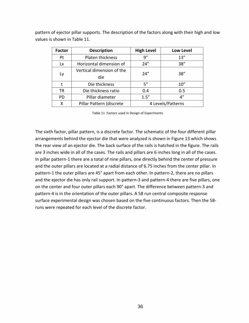
36
pattern of ejector pillar supports. The description of the factors along with their high and low
values is shown in Table 11.
Factor Description High Level Low Level
Pt Platen thickness 9” 13”
Lx Horizontal dimension of 24” 38”
Ly Vertical dimension of the
die 24” 38”
t Die thickness 5” 10”
TR Die thickness ratio 0.4 0.5
PD Pillar diameter 1.5” 4”
X Pillar Pattern (discrete 4 Levels/Patterns
Table 11 Factors used in Design of Experiments
The sixth factor, pillar pattern, is a discrete factor. The schematic of the four different pillar
arrangements behind the ejector die that were analyzed is shown in Figure 13 which shows
the rear view of an ejector die. The back surface of the rails is hatched in the figure. The rails
are 3 inches wide in all of the cases. The rails and pillars are 6 inches long in all of the cases.
In pillar pattern‐1 there are a total of nine pillars, one directly behind the center of pressure
and the outer pillars are located at a radial distance of 6.75 inches from the center pillar. In
pattern‐1 the outer pillars are 45° apart from each other. In pattern‐2, there are no pillars
and the ejector die has only rail support. In pattern‐3 and pattern‐4 there are five pillars, one
on the center and four outer pillars each 90° apart. The difference between pattern‐3 and
pattern‐4 is in the orientation of the outer pillars. A 58 run central composite response
surface experimental design was chosen based on the five continuous factors. Then the 58‐
runs were repeated for each level of the discrete factor.

37
Figure 13 Schematic of Pillar Patterns used in the Study
Pattern‐1, 9 pillars, (b) Pattern‐2, No pillars, (c) Pattern‐3, Five Pillars, (d) Pattern‐4, 5 pillars
The maximum cover and ejector side parting plane separation were predicted for each case
in the experimental array using the finite element modeling methodology
3.4.2 DimensionalAnalysisThe objective of the computational experiments is to develop empirical correlations to
predict the maximum parting plane separation as a function of the design variables involved.
Dimensional analysis was used to determine the non‐dimensional parameters for the
empirical correlations. Dimensional analysis is based on the principle that any valid physical
relationship should be dimensionally homogeneous. Based on this principle Buckingham [58]
showed in his famous Pi‐theorem that any equation describing the physical relationship
between the variables can be reformulated as a function of dimensionless products of
variables.

38
The choice of variables to be used in the dimensional analysis and the grouping of variables
that form the non‐dimensional groups can be determined using the knowledge of the
physical phenomenon and engineering judgment. The dies and inserts are assumed as pre‐
stressed flat plates that are resting on elastic supports and subjected to uniform loading. The
semi analytical empirical equation for predicting maximum deflection of a flat plat under
uniform loading is given by [60].
4
3
WLMaximum deflection
Et (4)
W is the uniformly distributed load, l is the length of the plate, E is the young’s modulus, t is
the plate thickness and α is a constant that depends on the aspect ratio and boundary
conditions. The unsupported span behind the cover die is characterized by the length and
width of the die and a model for cover side separation will take a form similar to the
deflection equation above. However on the ejector side the unsupported span is
characterized by the distance between the pillars and rail supports. Jofreit [61] developed a
semi empirical equation to predict the maximum deflection of concrete flat plates supported
on straight beams around the periphery and a grid of pillars in between the beam supports.
The equation to predict the maximum deflection within any inner grid of pillars is given by
4
3
3
4
s nl lW
Maximum deflectionEt
(5)
where ls and ln are the long span and the short span between the pillar supports. It can be
observed that the span variable L in equation (4) is replaced by the weighted average of the
shorter and longer span between the pillar supports. Therefore a model for the ejector side
separation will take a similar form. Based on the structure of the equations (4) and (5), the
physical relation between the maximum parting plane separation and the design variables
can be written as follows:
max , , , , , , , , , , 0 tb nf Pt L t TR L l PD RW DistributedLoad E (6)
where, δmax is the maximum parting plane separation, Ltb is the distance between the tie bar
centers, L is the length scale representing the length and width of the die or the span
between the pillars, ln is the length scale for span between pillars, PD is the pillar diameter,
RW is the width of the die and E is the young's modulus of the die material. The term
Distributed Load denotes the distributed contact load at the parting surface and it is
approximates as follows:

39
Pr Pr
-
x y x y
TotalClamp Load Cavity essure ojectedAreaofCavityDistrubted Contact Load
L L L L(7)
The non‐dimensional parameters selected are summarized as shown in Table 12. Details can
be found in Appendix A.
Dimensionless
Parameter
Description
П1 (Ltb/t) or (Distance between tie bar centers/Die thickness)
П2 (Pt/t ) or (Platen thickness/Die thickness)
П3 (TR) or (Die shoulder thickness/Die thickness)
П4 (L/t ) or (Span/Die thickness)
П5 (Max Separation/t)× (Young’s Modulus/Distributed contact
load)
П6 (Lx/Ly) or (Aspect ratio of the die)
П7 (Lcx/Lcy) or (Aspect ratio of the cavity)
Table 12 Non‐Dimensional Structural Design Parameters
The parameter П1, indicates that increasing the distance between the tie bar center has the
same effect as decreasing the die thickness. If the distance between the tie bars increases
for a given platen thickness, the platen bends more and the support available for the dies is
reduced and the dies deflect more. Decreasing the die thickness will also result in an
increase in the deflection of the die. Though the variable Ltb was not explicitly varied in the
computational experiments, the parameter П1 varies among the experimental cases due to
the variation in die thickness among the experimental cases and the effect of Ltb can be
captured from the computational experiments.
The second parameter П2 can be combined with the first parameter П1, to obtain a new non
dimensional parameter, say, П1‐2, which is given by
11 2
2
tb
Pt
L (8)
The parameter П1‐2, above shows that there is always a combination of values of platen
thickness and distance between tie bar centers for which the platen stiffness remains a
constant. The most important non dimensional parameter is П4 which represents the ratio
between the unsupported span and the die thickness. This parameter suggests that larger
the span behind the die, thicker should be the die. A combination of the span and die

40
thickness can always be chosen to obtain a desired magnitude of parting plane separation.
On the ejector side, the parameter П4 represents the ratio of the span between the pillar
supports to the die thickness. In our experiments the pillar locations with respect to the
center of pressure were fixed. But the thickness of the die was varied and hence the
parameter П4 varies among the different experimental cases. This enables the power law
model fit to capture the inherent variability in die deflection caused by changes in
unsupported span and die thickness.
Seven common length scales (L1x, L1y, L2, L3, L4, RWX and RWY) that characterize the span
between pillars in each pillar pattern were identified as shown in Figure 14 and a general
closed form expression that can be extended to any arbitrary pillar pattern was developed.
The model form used in the regression for the ejector side data is shown in equation (9)
below. The term Liavg represents the average of the internal spans (L2, L3 and L4) between
the pillar supports in each of the four pillar support cases. For pillar pattern‐1, Liavg was taken
to be the average of L2, L3 and L4. For pillar pattern‐2, there are no pillar supports and hence
Liavg was taken to be zero. For pattern‐3, Liavg is the average of L2 and L4 and for pillar pattern‐
4 it is the average of L3 and L4. The variable np was introduced as a correction for the
number of pillar supports.
The power law model was obtained by non linear regression using sequential quadratic
programming optimization algorithm in SPSS [67]. The parameter estimates, the standard
error values and the confidence intervals for the parameter estimates are shown in Table 13.
The resulting equation is shown in (10). The standard error values and the confidence
intervals were estimated using the linearized form of equation (9) and indicate a very good
fit.
71 61
43
1
6
8 0 1
1 12
2 2
1
cc cnp
tb
tb
cc
npiavg
c
LMax Ejector Sep E PTc c
t Dist load L t
LL x L y RWX RWYc
t t t
Lx Lcy
Ly Lcx
(9)

41
Parameter Estimates
Parameter EstimateStd.
Error
95%
Confidence
Interval
Lower
Bound
Upper
Bound
c0 26.586 6.25 14.261 38.91
c1 ‐0.954 0.1 ‐1.15 ‐0.758
c2 1.62 0.078 1.467 1.773
c3 3.785 0.113 3.563 4.008
c4 1.484 0.084 1.319 1.649
c5 ‐0.407 0.108 ‐0.62 ‐0.193
c6 ‐1.488 0.119 ‐1.722 ‐1.253
c7 3.053 0.354 2.356 3.751
c8 20.205 3.672 12.964 27.446
Adjusted R squared = 0.982.
Table 13 Parameter Estimates for Ejector Side Fit
3.1-0.95+ -1.51+np
tb
tb
1.53.8+
1+npiavg
-0.41
LMax Ejector Sep E Pt× =20.2+26.6 1+ × ×
t Dist load L t
LL1x+L1y RWX+RWY× + +1.6 ×
2t 2t t
Lx Lcy× 1+ ×
Ly Lcx
(10)

42
Figure 14 Length Scales Representing Unsupported Span
The largest contribution to the ejector side separation comes from the unsupported span
behind the die which is characterized by the number, size and location of the support pillars
and rails. The term ‘np’ in the exponent for the average span variable suggests that as the
number of pillars increases, the value of the exponent decreases and the separation
becomes less sensitive to the span between the pillars as opposed to case which has fewer
pillar supports. When ‘np’ decreases the value of the exponent increases and the model
prediction becomes more sensitive to the span between the pillars.
The next major variable affecting the separation on the ejector side is the thickness of the
die shoe. For a case with no pillar supports, the effect of die thickness on the maximum
ejector side separation is in the order, Ө (t ‐2.8) while all other factors are held constant.
Increasing the thickness of the die results in an increase in the stiffness of the die and hence
thicker the die, less the separation.
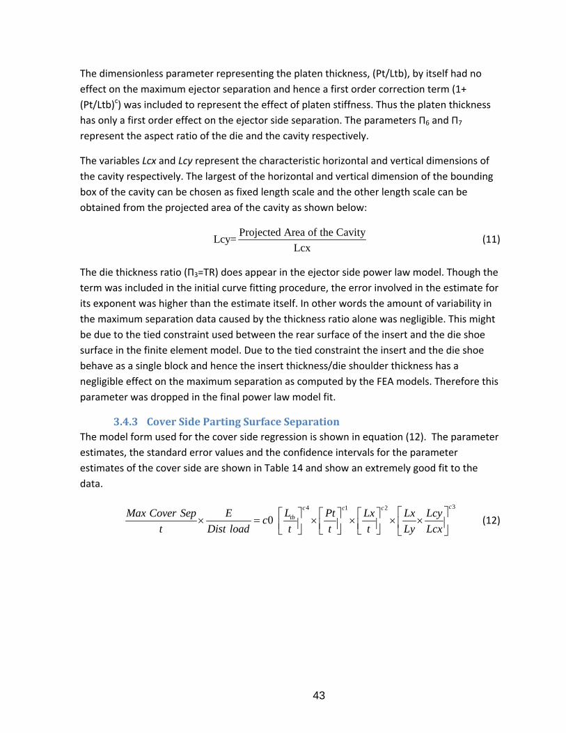
43
The dimensionless parameter representing the platen thickness, (Pt/Ltb), by itself had no
effect on the maximum ejector separation and hence a first order correction term (1+
(Pt/Ltb)c) was included to represent the effect of platen stiffness. Thus the platen thickness
has only a first order effect on the ejector side separation. The parameters П6 and П7
represent the aspect ratio of the die and the cavity respectively.
The variables Lcx and Lcy represent the characteristic horizontal and vertical dimensions of
the cavity respectively. The largest of the horizontal and vertical dimension of the bounding
box of the cavity can be chosen as fixed length scale and the other length scale can be
obtained from the projected area of the cavity as shown below:
Projected Area of the Cavity
Lcy=Lcx
(11)
The die thickness ratio (П3=TR) does appear in the ejector side power law model. Though the
term was included in the initial curve fitting procedure, the error involved in the estimate for
its exponent was higher than the estimate itself. In other words the amount of variability in
the maximum separation data caused by the thickness ratio alone was negligible. This might
be due to the tied constraint used between the rear surface of the insert and the die shoe
surface in the finite element model. Due to the tied constraint the insert and the die shoe
behave as a single block and hence the insert thickness/die shoulder thickness has a
negligible effect on the maximum separation as computed by the FEA models. Therefore this
parameter was dropped in the final power law model fit.
3.4.3 CoverSidePartingSurfaceSeparationThe model form used for the cover side regression is shown in equation (12). The parameter
estimates, the standard error values and the confidence intervals for the parameter
estimates of the cover side are shown in Table 14 and show an extremely good fit to the
data.
34 1 2
0
cc c c
tbLMax Cover Sep E Pt Lx Lx Lcyc
t Dist load t t t Ly Lcx (12)
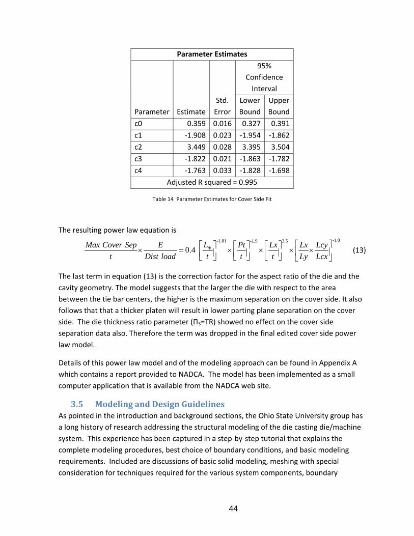
44
Parameter Estimates
Parameter Estimate
Std.
Error
95%
Confidence
Interval
Lower
Bound
Upper
Bound
c0 0.359 0.016 0.327 0.391
c1 ‐1.908 0.023 ‐1.954 ‐1.862
c2 3.449 0.028 3.395 3.504
c3 ‐1.822 0.021 ‐1.863 ‐1.782
c4 ‐1.763 0.033 ‐1.828 ‐1.698
Adjusted R squared = 0.995
Table 14 Parameter Estimates for Cover Side Fit
The resulting power law equation is
-1.8-1.81 -1.9 3.5
0.4
tbLMax Cover Sep E Pt Lx Lx Lcy
t Dist load t t t Ly Lcx (13)
The last term in equation (13) is the correction factor for the aspect ratio of the die and the
cavity geometry. The model suggests that the larger the die with respect to the area
between the tie bar centers, the higher is the maximum separation on the cover side. It also
follows that that a thicker platen will result in lower parting plane separation on the cover
side. The die thickness ratio parameter (П3=TR) showed no effect on the cover side
separation data also. Therefore the term was dropped in the final edited cover side power
law model.
Details of this power law model and of the modeling approach can be found in Appendix A
which contains a report provided to NADCA. The model has been implemented as a small
computer application that is available from the NADCA web site.
3.5 ModelingandDesignGuidelinesAs pointed in the introduction and background sections, the Ohio State University group has
a long history of research addressing the structural modeling of the die casting die/machine
system. This experience has been captured in a step‐by‐step tutorial that explains the
complete modeling procedures, best choice of boundary conditions, and basic modeling
requirements. Included are discussions of basic solid modeling, meshing with special
consideration for techniques required for the various system components, boundary

45
conditions and material properties, thermal analysis with industry standard software,
mechanical analysis with Abaqus, and post processing. This document was provided to
NADCA and it has been converted to an electronic document available from the NADCA web
site. The complete document is provided in Appendix E.
4. BenefitsAssessment
This new technology was predicted to result in an average energy savings of 2.03 trillion
BTU’s/year over a 10 year period. Current (2011) annual energy saving estimates over a ten
year period, based on commercial introduction in 2009, a market penetration of 70% by
2014 is 4.26 trillion BTU’s/year by 2019.
Along with these energy savings, reduction of scrap and improvement in casting yield will
result in a reduction of the environmental emissions associated with the melting and pouring
of the metal which will be saved as a result of this technology. The average annual estimate
of CO2 reduction per year through 2020 is 0.085 Million Metric Tons of Carbon Equivalent
(MM TCE).
Estimates of energy savings are based on the following assumptions:
‐ There was an estimated 1.6 million tons of die casting shipments in 2000 (U.S.
Department of Commerce, U.S. Census Bureau, Current Industrial Reports, Iron and
Steel Castings, MA331E (00)‐1.)
‐ The die casting industry will grow at a rate of2.5% per year (AFS Metalcasting
Forecast & Trends 2002 (Oct. 2001))
‐ Baseline energy consumption for die casting is 23.4 million Btu per ton = 6858kWh
‐ The results of this project will provide the ability to design better dies which will in
turn reduce scrap and improve operating efficiency in contributing to a combined 8%
improvement in energy efficiency.
Assumes 3412 Btu/kWh (Source: DOE/EIA, Monthly Energy Review)
Approximately 25% of scrap and 75% new material are used during melting. The average
price for Aluminum scrap in 2001 was .49 a pound or $980 a ton (Source: American Metal
Market). For new aluminum it cost about $.70 a pound or $1400 per ton. (Source: U.S.
Geological Survey, Mineral Commodity Summaries, Jan 2002) A majority of die castings are
aluminum therefore aluminum price data was used for these calculations

46
5. Commercialization
This work has been incorporated into NADCA’s Productivity Improvement Suite and much of
the work is already available. Specific commercialization activities:
The “How to Model the Die/Machine System” report is available from the NADCA web site and provides a detailed step‐by‐step tutorial to assist the industry in more easily applying this type of modeling technology.
The tie bar balance power law model and the parting plane separation power law model have both been converted to computer applications that can be downloaded from the NADCA website and serve as simple design tools that can be applied throughout the industry.
The tie bar balance power law model is a module within version 4 of the PQ2 program distributed by NADCA. PQ2 program is used to optimally match the die and machine to the requirements of the casting and the tie bar module provides additional data to ensure that the proposed setup of the machine and die will not impose unbalanced loading along with the problems so entailed.
This work has been reviewed twice a year in the NADCA Computer Modeling Task Group and once per year in the NADCA Research and Development Committee throughout the duration of the project. Both groups are composed of members of the industry and these vehicles provide a mechanism to disseminate information as it develops as well as provide guidance to the research.
6. Accomplishments
This work resulted in the improvements of modeling procedures used to represent the
casting/die interface which is very important in extending the structural modeling of the die
and machine to modeling the development of stresses in the cast part. The work also
formalized the modeling procedures and captured in simple power law models much of the
information gained over many years of modeling work.
The papers developed from this work are listed below:
A. Ragab, K. Kabiri‐Bamoradian, R. A. Miller,, “Part Distortion and Stress Prediction in Die
Casting Process: Sensitivity Analysis,” 108th Metal Casting Congress, Paper T01‐012,
North American Die Casting Association, Rosemont, Illinois, June 2004.
A. Garza‐Delgado, A. Ragab, K. Kabiri‐Bamoradian, R. A. Miller,, “Finite Element Modeling
of Die Casting Die Distortion by Coupled Fluid‐Thermal‐Structural Analysis,” 108th Metal
Casting Congress, Paper T01‐041, North American Die Casting Association, Rosemont,
Illinois, June 2004.
A. Ragab, . K. Kabiri‐Bamoradian, R. A. Miller, “Experimental Validation of Die
Deformation Modeling,” 108th Metal Casting Congress, Paper T01‐052, North American
Die Casting Association, Rosemont, Illinois, June 2004.

47
E. Arrambide, A. Ragab, K. Kabiri‐Bamoradian, R. A. Miller, “Modeling Influence of the Die
Casting Machine Components on Contact Load Between Dies and Platens, , Paper T05‐
011, NADCA Transactions 2005, North American Die Casting Association, Wheeling,
Illinois, April 2005.
K. Murugesan, A. Ragab, K. Kabiri‐Bamoradian, R. A. Miller, “Effect of Die, Cavity and
Toggle Locations on Tie bar Forces, Toggle Forces and Parting Plane Separation, Paper
T05‐013, NADCA Transactions 2005,North American Die Casting Association, Wheeling,
Illinois, April 2005.
K.S. Murugesan, A. Ragab, K. Kabiri‐Bamoradian and R. A. Miller, “A Model to Predict Tie
Bar Load Imbalance,” Paper T06‐121, NADCA Transactions 2006, North American Die
Casting Association, Wheeling, Illinois, April 2006
K. Murugesan, A. Ragab, K. Kabiri‐Bamoradian, R. A. Miller, “An Experimental Verification
of the Effect of Die, Locations on Tie Bar Load Imbalance, NADCA Transactions
2007,North American Die Casting Association, Wheeling, Illinois, May 2007.
K. Murugesan, K. Kabiri‐Bamoradian, R. A. Miller, “The Effect of Support Pillar Patterns
on the Mechanical Performance of the Ejector Side Dies", NADCA Transactions 2008,
North American Die Casting Association, Wheeling, Illinois, May 2008.
Abelardo Garza‐Delgado, K. Kabiri‐Bamoradian, R. A. Miller, “Determination of Elevated‐
Temperature Mechanical Properties of an Aluminum A380.0 Die Casting Alloy in the As‐
Cast Condition", NADCA Transactions 2008, North American Die Casting Association,
Wheeling, Illinois, May 2008.
R. A. Miller, K. Kabiri‐Bamoradian, and A. Garza, “Finite Element Modeling of Casting
Distortion in Die Casting,” NADCA Transactions 2009, North American Die Casting
Association, Wheeling, Illinois, April 2009
Two PhD Dissertations also derived from the work:
Abelardo Garza‐Delgado, “A Study of Casting Distortion and Residual Stresses in Die
Casting,” Industrial and Systems Engineering, The Ohio State University, 2007.
Karthik S. Murugesan, “Predicting Parting Plane Separation and Tie Bar Loads in Die
Casting Using Computer Simulation and Dimensional Analysis,” Industrial and Systems
Engineering, The Ohio State University, 2008.

48
7. Conclusions
The project has successfully extended the capability to model the die casting die/machine
system and has made the use of this technology more accessible to the industry. The state‐
of‐the‐art in the modeling of fluid‐structure interactions still does not allow us to adequately
model the casting/die interface during cavity filling and during solidification, but improved
approximations were developed.
The use of dimensional analysis to develop power law models for parting plane separation
and for tie bar loading turned out to be extremely effective. The resulting power law
functions turned out to be very accurate, certainly adequate, for the purposes of evaluating
the suitability of a proposed die design and die/machine setup. As part of the presentations
of the work before industry groups, we have made a point to encourage companies who
routinely perform process modeling to consider the general approach since it leverages the
results of specific simulations and helps to quantify, formalize and generalize lessons learned
from the specific simulation results thereby amplifying the benefit from the investment in
the technology.
8. Recommendations
While structural modeling of the die/machine system is relatively mature, extension of the
modeling to include the effects of the die and machine on the part dimensions and stress
state after cooling is not. There are still major issues in capturing the macroscopic behavior
of the casting/die interface during and immediately after filling. As the capabilities of
generic fluid structure interaction improve, perhaps the modeling of the casting properties
can be improved.
The second major impediment is the lack of high temperature material properties. The
mechanical properties of the cast alloy are needed up to the solidus temperature and over a
wide range of strain rates. Such data are virtually non‐existent today and must be
developed in the very near future.
49
9. References
[1] Chayapathi, A., 1999, "Study of the Effect of Structural Variables of Die and Die Casting
Machine on Die Deflections," Master’s Thesis, The Ohio State University.
[2] Kulkarni, Y., 2000, "Study of the Effect of Structural Variables of Die and Die Casting
Machine on Die Deflections," Master’s Thesis, The Ohio State University.
[3] Tewari, A., 2000, "Study of the Effect of Structural Variables of Die and Die Casting
Machine on Die Deflections," Master’s Thesis, The Ohio State University.
[4] Miller, R.A., 2003, "Die Deflection Modeling: Empirical Validation and Tech Transfer," US
Department of Energy Project Report, Project DE‐FC07‐97ID13576.
[5] Herman, E.A., 1992, "Designing die casting dies," North American Die Casting Association,
Rosemont, IL, USA.
[6] Hetu, J. F., Gao, D. M., Kabanemi, K. K., 1998, "Numerical Modeling of Casting Processes,"
Advanced Performance Materials, 5pp. 65‐82.
[7] Barone M.R., Caulk D.A., 2000, "Analysis of Liquid Metal Flow in Die Casting,"
International Journal of Engineering Science., 38(12) pp. 1279‐1302.
[8] Jia, L., Xiong, S., and Liu, B., 2000, "Study on Numerical Simulation of Mold Filling and
Heat Transfer in Die Casting Process," Journal of Material Science and Technology, 16(3) pp.
269‐272.
[9] Kulasegaram, S., Bonet, J., Lewis, R. W., 2003, "High Pressure Die Casting Simulation using
a Lagrangian Particle Method," Communications in Numerical Methods in Engineeering,
19pp. 679‐687.
[10] Cleary, P., Ha, J., Alguine, V., 2002, "Flow Modelling in Casting Processes," Applied
Mathematical Modelling, 26pp. 171‐190.
[11] Bounds, S., Davey, K., and Hinduja, S., 1999, "Modelling the Pressure Die Casting Process
using a Hybrid Finite‐Boundary Element Model," International Journal of Numerical Methods
in Engineering, 45pp. 1165‐1185.

50
[12] Xiong, S. M., Lau, F., Lee, W. B., 2003, "Numerical Methods to Improve the
Computational Efficiency of Thermal Analysis for the Die Casting Process," Journal of
Materials Processing Technology, 139pp. 457‐461.
[13] Koric, S., and Thomas, B. G., 2006, "Efficient Thermo‐Mechanical Model for Solidification
Processes," International Journal of Numerical Methods in Engineering, 66pp. 1955‐1989.
[14] Song, Y., Yan, Y., Zhang, R., 2001, "Three Dimensional Non‐Linear Coupled Thermo‐
Mechanical FEM Analysis of the Dimensional Accuracy for Casting Dies in Rapid Tooling,"
Finite Elements in Analysis and Design , 91, 38pp. 79‐91.
[15] Dour, G., 2001, "Thermal Stresses and Distortion in Dies of Die Casting Processes: A New
Normalized Approach," Modelling and Simulation in Materials Science and Engineering, 9(5)
pp. 399‐413.
[16] Broucaret, S., Michrafy, A., and Dour, G., 2001, "Heat Transfer and Thermo‐Mechanical
Stresses in a Gravity Casting Die," Journal of Materials Processing Technology, 110(2) pp.
211‐217.
[17] Lin, J. C., 2003, "The Optimal Design of a Cooling System for a Die‐Casting Die with a
Free Form Surface," The International Journal of Advanced Manufacturing Technology, 21(8)
pp. 612‐619.
[18] Srivastava, A., Joshi, V., and Shivpuri, R., 2004, "Computer Modeling and Prediction of
Thermal Fatigue Cracking in Die‐Casting Tooling," Wear, 256(1‐2) pp. 38‐43.
[19] Sakhuja, A., and Brevick, J. R., 2004, "Prediction of Thermal Fatigue in Tooling for Die‐
Casting Copper Via Finite Element Analysis," Proceedings of the 8th International Conference
on Numerical Methods in Industrial Forming Processes, 712(1) pp. 1881‐1886.
[20] Park, J. K., Samarasekara, I. V., Thomas, B. G., 2000, "Analysis of thermal and
mechanical behavior of copper mould during thin slab casting," 83rd Steelmaking
Conference Proceedings, 83, pp. 9‐21.
[21] Ahuett‐Garza, H., 1996, "Characterization of Loads in Die Casting and Prediction of Die
Deflections," PhD Dissertation, The Ohio State University.
[22] Ahuett‐Garza, H.,Miller, 1997, "NADCA‐Sponsored Research: Computer Simulation of
Causes and Effects," NADCA Transactions, pp. 41‐48.

51
[23] Ahuett‐Garza, H., and Miller, R. A., 2003, "The Effects of Heat Released during Fill on the
Deflections of Die Casting Dies," Journal of Materials Processing Technology, 142(3) pp. 648‐
658.
[24] Hegde, K., Ahuett‐garza, H., Padiyar, G., 1995, "NADCA‐Sponsored Research: FEM
analysis of die casting die deflections: Part I‐ Modeling and Simualtion," NADCA Transactions,
pp. 17‐23.
[25] Ahuett‐Garza, H., Hegde, K., Padiyar, G., Miller,R.A., 1995, "NADCA‐Sponsored Research:
FEM analysis of die casting die deflections: part II, results," NADCA Transactions, pp. 25‐31.
[26] Dedhia, S., Ahuett‐Garza, H., Miller, R. A., 1997, "NADCA Sponsored Research: Analysis
of Proud Inserts on Die Deflections and Slide Blow Back in Die Casting Dies," NADCA
Transactions, pp. 35‐40.
[27] Choudhry, A. K., Dedhia, S., Ahuett‐Garza, H., 1997, "NADCA Sponsored Research: Study
of the Effect of Platen Size on Clamping Characteristics of Die," NADCA Transactions, pp.
103‐106.
[28] Chayapathi, A., Kesavan, V., and Miller, R. A., 1999, "The effects of structural die and
machine variables on die deflections," NADCA Transactions.
[29] Ragab, A., Kabiri‐Bamoradian, K., and Miller, R. A., 2004, "Experimental validation of die
deformation modeling," NADCA Transactions.
[30] Arrambide, E., Ragab, A., Kabiri‐Bamoradian, K., 2005, "Modeling Influence of the Die
Casting Machine Components on Contact Load between Dies and Platens," NADCA
Transactions.
[31] Garza‐Delgado, A., Ragab, A., Kabiri‐Bamoradian, K., 2004, "Finite element modeling of
die casting die distortion by coupled fluid‐thermal‐structural analysis," NADCA transactions.
[32] Xue, H., Kabiri‐Bamoradian, K., and Miller, R. A., 2005, "Modeling the dynamic cavity
pressure and impact spike in die casting," NADCA Transactions.
[33] Miller, R. A., and Arrambide, A., 1999, "Finite element modeling of slide distortion in
transmission casing die," NADCA Transactions.
[34] Vashisht, A., Kabiri‐Bamoradian, K., and Miller, R. A., 2002, "Die Casting Die Distortion:
Case Study to Predict Parting Plane Separation and Flash Location," NADCA Transactions, pp.
1‐6.
52
[35] Flynn, E. W., and Douglas, S., 2005, "Real time defelction measurement," NADCA
Transactions.
[36] Garza‐Delgado, A., Miller, R. A., and Kabiri‐Bamoradian, K., 2003, "Using die
deformation modeling to predict component failure in a miniature zinc die," NADCA
Transactions, pp. 25‐33.
[37] Milroy, J., Hinduja, S., and Davey, K., 1998, "Modelling the Pressure Die Casting Process
with the Boundary Element Method: Die Deformation Model for Flash Prevention,"
Proceedings of Instituion of Mechanical Engineers, 212 Part Cpp. 197‐215.
[38] Alonso Rasgado, M. T., Davey, K., Clark, L. D., 2006, "Boundary Element Stress Analysis
for Copper‐Based Dies in Pressure Die Casting," Computers and Structures, 84(3‐4) pp. 254‐
267.
[39] Barone, M. R., and Caulk, D. A., 1999, "Analysis of thermo mechanical distortion in die
casting," ," NADCA Transactions, pp. 81‐89.
[40] Ragab, A., Kabiri‐Bamoradian, K., and Miller, R. A., 2001, "Modeling part distortion and
stresses in die casting," NADCA Transactions, pp. 77‐83.
[41] Ragab, A., Kabiri‐Bamoradian, K., and Miller, R. A., 2004, "Part distortion and stress
prediction in die casting process: Sensitivity analysis," NADCA Transactions.
[42] Garza‐Delgado, A., Kabiri‐Bamoradian, K., and Miller, R. A., 2007, "Finite element
modeling of casting distortion in die casting," NADCA transactions.
[43] Jayaraman, P., 1999, "Finite Element Modeling and Parametric Study of Slide Deflection
in a Die Casting Die with an Inboard Lock Design," Master’s Thesis, The Ohio State University.
[44] Chakravarthi, V., 2000, "Parametric Deflection Study and Fatigue Life Prediction of Non
Open‐Close Die Components," Master’s Thesis, The Ohio State University.
[45] Miller, R. A., Chakravarthi, V., Kabiri‐Bamoradian, K., 2001, "Modeling the distortion and
mechanical performances of dies," NADCA Transactions.
[46] Dedhia, S., 1997, "Study of the Effect of Structural Variables of Die on Die Deflections,"
Master’s Thesis, The Ohio State University.
[47] Isayev, A. I., Scavuzzo, R. J., and Kuroyama, Y., 1994, "Injection Molding of Rubber
Compounds: Cavity Filliung, Packing and Flash Formation," Journal of Applied Polymer
Science: Applied Polymer Science Symposium, 53pp. 233‐252.

53
[48] Chen, Z., Giacomin, J. A., and Turng, L., 2006, "Flash," Polymer Engineering & Science,
46pp. 241‐247.
[49] Carpenter, B., Patil, S., Hoffman, R., 2006, "Effect of Machine Compliance on Mold
Deflection during Injection and Packing of Thermoplastic Parts," Polymer Engineering &
Science, 46(7) pp. 844‐852.
[50] Hostert, C., Kollmeier, H., Maas, S., 2004, "Simulation of locking mechanism of an
injection moulding clamp unit," NAFEMS Seminar: Analysis of Multi Body Systems using FEM
and MBS, Oct 27‐28, 2004, Weisbaden, Germany.
[51] Beiter, K. A., Cardinal, J. M., and Ishii, K., 1995, "Design for Injection Molding: Balancing
Mechanical Requirements, Manufacturing Costs and Material Selection," Proceedings of the
ASME Symposium on Design for Manufacture.
[52] Menges, Michaeli, and Mohren., 2000, "How to make injection molds," Third Edition,
Hanser Gardner Publications, Cincinnati.
[53] Sasikumar, C., Srikanth, S., and Das, S. K., 2006, "Analysis of Premature Failure of a Tie
Bar in an Injection Molding Machine," Engineering Failure Analysis, 13(1246) pp. 1259.
[54] Simpson, T. W., Poplinski, J. D., Koch, P. N., 2001, "Metamodels for Computer‐Based
Engineering Design: Survey and Recommendations," Engineering with Computers, 17(2) pp.
129‐150.
[55] W. J. Roux, Nielen Stander,R.T.Haftka, 1998, "Response Surface Approximations for
Structural Optimization," International Journal for Numerical Methods in Engineering, 42(3)
pp. 517‐534.
[56] Sacks, J., Welch, W. J., Mitchell, T. J., 1989, "Design and Analysis of Computer
Experiments," Statistical Science, 4(4) pp. 409‐423.
[57] ABAQUS Version 6.6, User’s Guide.
[58] Buckingham, E., 1914, "On Physically Similar Systems; Illustrations of the use of
Dimensional Equations," Physical Review, IV(4) pp. 345‐376.
[59] Vignaux, V. A., and Scott, J. L., 1999, "Simplifying Regression Models using Dimensional
Analysis," Australian & New Zealand Journal of Statistics, 41(1) pp. 31‐41.
[60] Roark, R.J., and Young, W.C., 1975, "Formulas for stress and strain," Fifth Edition,
McGraw‐Hill, New York.

54
[61] Jofriet, J. C., 1973, "Short Term Deflections of Concrete Flat Plates," Journal of the
Structural Division, 99(1) pp. 167‐182.
[62] Buckingham, E., 1915, "Model Experiments and the Forms of Empirical Equations,"
Transactions of ASME, 37pp. 263‐294.
[63] Allen, T. T., and Yu, L., 2002, "Low‐Cost Response Surface Methods from Simulation
Optimization," Quality and Reliability Engineering International, 18(1) pp. 5‐17.
[64] Allen, T. T., Yu, L., and Schmitz, J., 2003, "An Experimental Design Criterion for
Minimizing meta–model Prediction Errors Applied to Die Casting Process Design," Journal of
the Royal Statistical Society, 52(1) pp. 103‐117.
[65] Murugesan, K. S., Ragab, A., Kabiri‐Bamoradian, K., and Miller, R.A., 2006, "A Model to
Predict Tie Bar Load Imbalance," NADCA Transactions.
[66] Vinarcik, E. J., 2003, "High Integrity Die Casting Process," John Wiley & Sons
Publications, New York
[67] SPSS Regression Models 16.0, User’s Manual.
55
10. AppendicesA–E
Appendix A: Die and Die Casting Machine Force and Deflection Predictions
Appendix B: Door Closer Die Case Study
Appendix C: Finite Element Modeling of Casting Distortion in Die Casting
Appendix D: Determination of Elevated Temperature Mechanical Properties of an
Aluminum A380.0 Die Casting Alloy in As‐Cast Condition
Appendix E: Die and Die Casting Machine Computer Simulations: Modeling, Meshing,
Boundary Conditions, and Analysis Procedures

Appendix A: Die and Die Casting Machine Force and Deflection
Predictions
DieandDieCastingMachineForceandDeflectionPredictions:
CorrelationsforPredictingTieBarForcesandPartingPlaneSeparation
Khalil Kabiri-Bamoradian
Center for Die Casting The Ohio State University
April 2009

i
Summary
Die casting is used to produce complex parts generally in large volumes and it can produce
parts with tight dimensional tolerances. The goal of many engineers who design engineered
parts is to have net-shape parts with no machining that can meet the engineering
specifications, tolerances, flatness and durability requirements of the parts. Computer
simulation has been used to help the die and part designers to design better dies and parts by
incorporating models of the die casting machine, dies, inserts, die supports and part as a
system analyzed together. Inclusion of a relatively accurate model of die casting machine is
essential for the prediction of the parting plane separation and tie bar loads.
Analytical equations or empirical correlations can be very useful tools to engineers and die
designers for predicting parting plane separation and tie bar loads at the initial stages of
design. The correlations are easy and quick to use and are very useful as long as they can give
a good predictions. These correlations can guide engineers and designers to design better dies
for the die casting machine to be used and also can provide guidance on the relative size of
die, size and pattern of pillar support for dies and the effect of the location of the die on
machine on part properties.
With this in mind, the Center for Die Casting at The Ohio State University has focused not
only on developing comprehensive computer models of part, dies, inserts, support frame,
support pillars and die casting machine (which includes platens, tie bars, toggle mechanism,
and machine base) that represents and simulate closely the actual die casting process set up,
the center has also developed regression models based on the results of the simulation runs.
The current proposed empirical correlations are based on dimensionless parameters that were
derived from the geometry of the part, die, inserts, pillars and machine and tie bars and
applied tie bar and intensification loads. Non-dimensional analyses were utilized to get the
dimensionless parameters. Two design of experiment (DOE) matrices were developed and
used, one for tie bar force computer simulation and another one for parting pane separation.
The DOE matrix for tie bar force predictions had 70 runs. Die thickness, die size in

ii
horizontal and vertical directions, center of die and center of pressure in vertical and
horizontal directions, thickness ratio of die and insert, and also the intensification pressure
were all varied in the DOE matrix. The simulation model was based on a 800 ton machine.
One of the computer simulation results was the resulting force in each tie bar. The DOE
matrix for parting plane separation had 232 runs. Platen thickness, die thickness, die size in
vertical and horizontal, support pillar diameter, thickness ratio of the die and insert and pillar
patterns were all varied. Four different pillar patterns were used in the run matrix. Non-linear
regression models using dimensionless parameter were fit to the results to get the empirical
correlations.
Two correlations were developed for the tie bars, one for top tie bars and another one for
bottom tie bars. The physical reason for having two correlations is that the bottom tie bar
forces are influenced by its proximity to the machine base where the cover platen is attached
to the machine; whereas the top tie bar does not have this condition. These equations are:
c1 c2
tb tb
tb tb
Top Tie bar load DPX DPYc0 1 1
Nominal Load 0.5L 0.5L
CPR A CPX CPY CPR A1 c3 exp 1 c4 1
CLAMP 0.5L 0.5L CLAMP
CPR A1 c5
CLAMP
CPR Aexp
CLAMP
c1 c2
tb tb
tb tb
Bottom Tie bar load DPX DPY0 1 1
Nominal Load 0.5L 0.5L
CPR A CPX CPY CPR A1 c3 exp 1 c4 1
CLAMP 0.5L 0.5L CLAMP
CPR A1 c5
CLA
c
CPR Aexp
MP CLAMP
Table 1 gives the description of parameter for the tie bar loads equations.

iii
Description
LX Die Width
LY Die Height
DPX Die location in X‐direction
DPY Die location in Y‐direction
CPX Location of center of pressure in X‐direction
CPY Location of center of pressure in Y‐direction
CPR Cavity Pressure
Table S-1, Tie Bar Correlations Parameters
Two correlations were also developed for the parting plane separation, one for the cover side
and another one for the ejector side. The physical reason for having two correlations is that
the ejector side has the ejector mechanisms and to give better support and to accommodate
ejector mechanism there is a support frame and support pillars behind the ejector die. Also,
the cover platen is attached to the base, whereas ejector platen can slide on the tie bars. The
pillar support pattern also depends on the die design, cooling lines, and the availability of
space. These two correlations are:
1.81.81 1.9 3.5Max Cover Sep E Ltb PT Lx Lx Lcy
0.4 t Dist load t t t Ly Lcx
3.10.95 1.5
1 np
1.53.8
1 npiavg
0.41
Max Ejector Sep E PT Ltb20.2 26.6 1
t Dist load Ltb t
LL1x L1y RWX RWY1.6
2t 2t t
Lx Lcy1
Ly Lcx

iv
Where Liavg is average length among the pillars and given by 2 3 niavg
L L ....... LL
n
where L2, L3, …,Ln are distances between pillars. The description of parameters for separation
correlations are given in Table 2.
Description
PT Platen thickness
Lx Horizontal dimension of the die
Ly Vertical dimension of the die
t Die thickness
TR Die thickness ratio
PD, np Pillar diameter, Number of pillars
Ltb Distance between tie bars
RWX, RWY Rail thickness in X and Y
L1X, L1Y Distance between rails in X and Y
Table 2 Parting Plane Separation Correlations Parameters.
The correlations for tie bar forces were compared against available computer simulations for
die casting machines of 250, 800 and 3000 tons. The percent tie bar load imbalance prediction
from the correlation and computer simulation for these machines for top and bottom tie bars
were within 2-5%. A comparison was also made with measured data from an experiment.
The experimental data were collected using the 250 ton machine at the Center for Die
Casting. The percent imbalance from the correlation prediction and actual experimental data
were within 0-10 percent depending on die location with some of the deviation possibly
attributed to lack of squareness and parallelism of this machine.
The correlations for the parting plane separation for cover side and ejector side were verified
against three more computer simulations with different pillar patterns. The comparison
showed that the maximum difference between the correlation perditions and computer
simulation were 0.0005” on the cover side and 0.002’’ on the ejector side. Also steps and

v
procedure were developed to find equivalent stiffness of cover and ejector platens for designs
other than those used in the simulations
In conclusions, the proposed empirical correlations for the tie bar force and parting plane
separation predictions give extremely good results and they have been compared with
different machine designs, die designs and pillar patterns.

vi
Contents
Summary ...................................................................................................................................... i
1. Introduction ......................................................................................................................... 1
2. Force Path and Machine/Die Stiffness ................................................................................ 3
3. Spring–Force Circuit of dies and Die casting Machine ...................................................... 4
3.1 Example of Machine and Die Stiffness ....................................................................... 6
4. Tie Bar forces and Parting Plane Separation of Dies .......................................................... 8
4.1 Tie Bars Force Distribution from Clamp Force ........................................................... 8
4.2 Intensification Pressure .............................................................................................. 10
4.3 Parting Plane Separation of Dies ............................................................................... 11
5. Correlations to Predict Tie Bar Forces .............................................................................. 12
6. Correlation to Predict Cover Side and Ejector Side Parting Plane Separation ................. 19
6.1 Rules to Characterize the Spans Between Pillars and the Spans Between Pillars and
Rails 30
7. Equivalent Machine Stiffness ........................................................................................... 31
7.1 Steps to Determine Equivalent Cover Platen Thickness ........................................... 32
7.2 Steps to Determine Equivalent Ejector Platen Thickness .......................................... 36
7.3 Steps to Determine Equivalent Ejector Platen Thicknesses with Different Toggle
Locations .............................................................................................................................. 38
8. References ......................................................................................................................... 40

1
1. Introduction
The die casting process is used to produce complex parts generally in large volumes and with
tight tolerances. The goal of many engineers who design engineered parts is to have net-shape
parts that require no machining and that meet the engineering specifications, tolerances,
flatness and durability test requirements. In order to reach these goals part designers, die
designers and process engineers should consider the parameters of the dies and machines that
will influence the part’s geometrical dimensions and its mechanical and thermal performance.
The dies/inserts, machine and part all experience loads due to clamp, intensification, thermal
and dynamic phenomena [1, 2, 3]. The clamp force and intensification loads are relatively
consistent from cycle to cycle while the thermal loads change from cycle to cycle and may
reach a quasi-steady state only after many (100-150) cycles [4, 5, 6]. The dynamic loads are
generated by acceleration and deceleration of the moving parts, such as plunger, plunger rod,
liquid metal and hydraulic system and liquids [7].
These loads can be simulated using steady state static analysis. The clamp and intensification
loads as mentioned before are fixed for all cycles. A transient thermal analysis of dies, inserts
and parts and possibly platens, if necessary, should be run before the static analysis. The
output of the analysis is the nodal temperature at each cycle [5, 7]. Thermal loads can be
added to clamp and intensification loads by selecting thermal loads from the transient thermal
analysis. At the Center for die casting thermal loads selected are usually cycle one, cycle 30
and cycle 100. A simple way to simulate the dynamic loads is by multiplying the
intensification loads by a factor determined from the machine characteristics, This factor can
vary from 1.5 to 2.5 [7].
The present article will discuss the effect of clamp and intensification loads on the tie bar
forces and parting plane separation. The thermal loads are not considered here [8, 20]. The
objective of this study was to determine how these two loads influence the tie bar forces and
parting plane separation.
Tie bar loads and parting plane separation are influenced by the die and machine dimensions,
shape and relative location, physical properties and the clamp and intensification forces [6, 8

2
,9 10, 11,12 , 18,19, 20]. The approach which was adopted for this report was to determine
non-dimensional numbers (a group of factors or variables) using the PI-Theorem and
determine the non-linear functional relation between these non-dimensional parameters/
numbers [8, 13, 14, 15] using a best-fit optimization procedure. The functional forms of these
correlations render themselves to combinations of power law and exponential functions. The
power laws and exponential functional forms in general are the solutions to governing non-
linear deferential equations. Therefore the use of these forms of equations in conjunction with
the non-dimensional variables results in empirical regression models that can be similar to,
and may be close to, the analytical forms derived from governing equations. The results will
therefore have a wider range of application than the domain used in original design of
experiments [8, 13,14,15]. Linear regression models which use polynomials have limited
scope and can be used only in the domain over which they have been developed and this
limits their use and application [16, 17, 18, 21]. Comparisons between the power law model
predictions and experiments and/or computer simulation with variables outside the range used
to derive the power law models confirm the above statements [8, 18, 19, 2].
The Section 1 of this article describes the force path in the die and the die casting machine.
Section 2 details a simple spring-force model which represents the die and machine stiffness.
Section 3 describes die and machine variables that affect the tie bar force and parting plane
separation. Sections 4 and 5 give the correlations for tie bars loads, parting plane separations.
Section 6 describes equivalent stiffness models for die and machine that can be used in the
correlations.
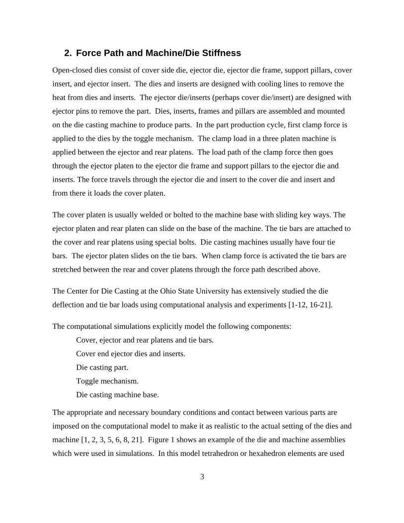
3
2. Force Path and Machine/Die Stiffness
Open-closed dies consist of cover side die, ejector die, ejector die frame, support pillars, cover
insert, and ejector insert. The dies and inserts are designed with cooling lines to remove the
heat from dies and inserts. The ejector die/inserts (perhaps cover die/insert) are designed with
ejector pins to remove the part. Dies, inserts, frames and pillars are assembled and mounted
on the die casting machine to produce parts. In the part production cycle, first clamp force is
applied to the dies by the toggle mechanism. The clamp load in a three platen machine is
applied between the ejector and rear platens. The load path of the clamp force then goes
through the ejector platen to the ejector die frame and support pillars to the ejector die and
inserts. The force travels through the ejector die and insert to the cover die and insert and
from there it loads the cover platen.
The cover platen is usually welded or bolted to the machine base with sliding key ways. The
ejector platen and rear platen can slide on the base of the machine. The tie bars are attached to
the cover and rear platens using special bolts. Die casting machines usually have four tie
bars. The ejector platen slides on the tie bars. When clamp force is activated the tie bars are
stretched between the rear and cover platens through the force path described above.
The Center for Die Casting at the Ohio State University has extensively studied the die
deflection and tie bar loads using computational analysis and experiments [1-12, 16-21].
The computational simulations explicitly model the following components:
Cover, ejector and rear platens and tie bars.
Cover end ejector dies and inserts.
Die casting part.
Toggle mechanism.
Die casting machine base.
The appropriate and necessary boundary conditions and contact between various parts are
imposed on the computational model to make it as realistic to the actual setting of the dies and
machine [1, 2, 3, 5, 6, 8, 21]. Figure 1 shows an example of the die and machine assemblies
which were used in simulations. In this model tetrahedron or hexahedron elements are used
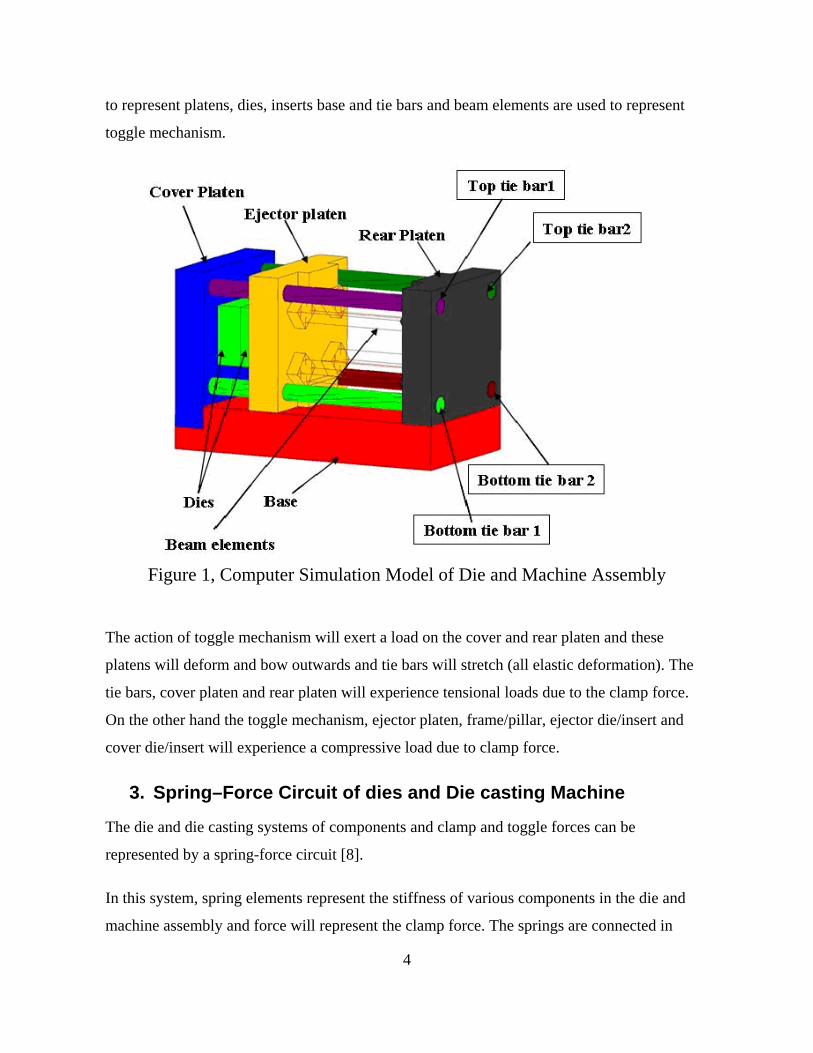
4
to represent platens, dies, inserts base and tie bars and beam elements are used to represent
toggle mechanism.
Figure 1, Computer Simulation Model of Die and Machine Assembly
The action of toggle mechanism will exert a load on the cover and rear platen and these
platens will deform and bow outwards and tie bars will stretch (all elastic deformation). The
tie bars, cover platen and rear platen will experience tensional loads due to the clamp force.
On the other hand the toggle mechanism, ejector platen, frame/pillar, ejector die/insert and
cover die/insert will experience a compressive load due to clamp force.
3. Spring–Force Circuit of dies and Die casting Machine
The die and die casting systems of components and clamp and toggle forces can be
represented by a spring-force circuit [8].
In this system, spring elements represent the stiffness of various components in the die and
machine assembly and force will represent the clamp force. The springs are connected in

5
series and/or parallel depending on how they interact with other components. Figure 2 shows
a simple equivalent spring-force circuit for the given simulation model. In figure 2 the
stiffness values are:
KRP Stiffness of Rear Platen,
KTB Stiffness of Tie Bars,
KCP Stiffness of Cover Platen,
KTG Stiffness of Toggle Mechanism,
KEP Stiffness of Ejector Platen,
KED Stiffness of Ejector Die,
KCD Stiffness of Cover Die,
KCPS Stiffness of Cover Die Parting Surface
KEPS Stiffness of Ejector Die Parting Surface
KPS Stiffness of Die Parting Surface (from KCPS and KEPS)
Figure 2, Spring-Force Elements for Clamp Load
The stiffness of each part can be calculated or can be derived from a simulation model. To
calculate stiffness from the simulation model an average of the actual displacement or
deformation of each component is calculated after removing pseudo-solid free motion
(translation) of the dies and platens. When clamp force is activated by the toggle mechanism,
the tie bars stretch and, due to this stretching, the dies and platens move and are displaced.
This translation is a pseudo free body motion, and it will not cause any stresses or

6
deformation. To calculate the actual deformation of these parts, this translation should be
removed from the given deformation results of the finite element simulation. An average
deflection of each component is estimated and used in calculation of stiffness of each
component K.
ClampFK
X
Where, ΔX is the average displacement and K is the stiffness of the component, and FClamp is
the clamp force value. The equivalent stiffness of the system in Figure 2 is:
A CP TB RP
B TG EP ED EPS CPS CD
eq A B
1 1 1 1
K K K K
1 1 1 1 1 1 1
K K K K K K K
K K K
KPS , the parting surface stiffness, can be calculated from the simulation results or from the
correlations to predict the maximum die separation, which will be discussed later in this
paper.
These equations provide a relatively straightforward way to compare machine and die
components.
3.1 Example of Machine and Die Stiffness
The machine stiffness and stiffness for two die designs are calculated to demonstrate how the
overall stiffness of die and machine will change depending on the die design [8].
In this example the machine configuration remains the same for both die designs while the
footprint of the dies is modified. One die has 24“ x 24” foot print and is 5’ thick while the
other die has a 36” x 36” footprint and is 5” thick. Table 1 shows the calculated stiffness for
each components of both assemblies and also shows the equivalent, or total stiffness of the
assembly,

7
Component Stiffness (N/m)
24" by 24” foot print, 5"
thick Die
38" by 38” foot print, 5"
thick Die
Rear Platen 2.3000E+10 2.3000E+10
Tie Bar 8.2000E+09 8.2000E+09
Cover Platen 3.0000E+10 3.0000E+10
Toggle 2.6000E+10 2.6000E+10
Ejector Platen 2.4000E+12 2.4000E+12
Ejector Die 7.4000E+11 2.5000E+11
Ejector Parting Surface 1.2251E+12 2.0000E+11
Cover Parting Surface 1.1568E+12 1.8000E+11
Cover Die 1.1400E+12 1.7100E+11
KA 5.03E+09 5.03E+09
KB 2.34E+10 1.69E+10
Equivalent Stiffness 2.84E+10 2.19E+10
Table 1, Stiffness Table for a machine and two die design
As can be seen from Table 1, the die with smaller footprint has a larger parting surface and
die stiffness resulting in a larger total stiffness than the die with the larger footprint with the
same thickness on the same machine. Therefore under the same forces, the larger foot print
die will have a larger deflection than the smaller one. To compensate for the lower overall
stiffness of the larger die, for example, the die thickness could be made thicker to increase the
stiffness to the same level of the smaller die.
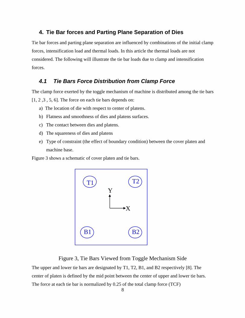
8
4. Tie Bar forces and Parting Plane Separation of Dies
Tie bar forces and parting plane separation are influenced by combinations of the initial clamp
forces, intensification load and thermal loads. In this article the thermal loads are not
considered. The following will illustrate the tie bar loads due to clamp and intensification
forces.
4.1 Tie Bars Force Distribution from Clamp Force
The clamp force exerted by the toggle mechanism of machine is distributed among the tie bars
[1, 2 ,3 , 5, 6]. The force on each tie bars depends on:
a) The location of die with respect to center of platens.
b) Flatness and smoothness of dies and platens surfaces.
c) The contact between dies and platens.
d) The squareness of dies and platens
e) Type of constraint (the effect of boundary condition) between the cover platen and
machine base.
Figure 3 shows a schematic of cover platen and tie bars.
Figure 3, Tie Bars Viewed from Toggle Mechanism Side
The upper and lower tie bars are designated by T1, T2, B1, and B2 respectively [8]. The
center of platen is defined by the mid point between the center of upper and lower tie bars.
The force at each tie bar is normalized by 0.25 of the total clamp force (TCF)
T1 T2
B2 B1
X
Y

9
If the dies are located at the center of platen and the surfaces are all flat and smooth and in
perfect contact, and if there is no effect of the boundary condition between the cover platen
and machine base, then all tie bars will carry equal forces, therefore:
1 2 1 2
1O.25*TCF O.25*TCF O.25*TCF O.25*TCF
T T B B
This means that all tie bars carry a normalized load of 1.00 or 100 percent.
In actual machines the cover platen is welded or it is bolted with key ways to the machine
base. Therefore due to the constraint (or effect of boundary condition) between the cover
platen and base, the tie bar loads will not be equal. In these cases B1 and B2 will carry higher
loads than T1 and T2.
The computer simulations at the Center for Die Casting show that the effect of boundary
conditions on tie bar load distribution is around 2-3 %. For example, simulation shows that
for dies centered on the platen the clamp load is approximately distributed among tie bars by
T1=T1= 0.99, B1=B2=1.01. It should be reminded that in these simulations due the nature of
Finite Element Analysis it is assumed that dies and platens are smooth, have perfect contact,
and dies and platens are square.
If the die is off center only in vertical direction, (Y direction, see Figure 3), with respect to the
center of the platen, the tie bars closest to the die will carry more forces than others. For
example if the dies are moved upward (positive Y) T1 and T2 will carry more load than B1
and B1.
If the dies are off centered with respect to platen center in both the X and Y directions, see
Figure 3, then the tie bar closet to the die will carry the most force and the tie bar farthest will
carry the least force. For example, if the dies move in positive Y and X , Figure 3, the closet
tie bar will be T2 which will carry highest force, and the farthest will be B1 which will carry
lowest force.

10
4.2 Intensification Pressure
When intensification pressure is applied to the cavity, the force generated by the cavity
pressure is distributed on the die and tie bars [1, 2, 3, 5, 6, 8,21]. The load path of the cavity
pressure is though cover and ejector dies to cover and ejector platens.
a b
Figure 4, Clamp and cavity Pressure
Figure 4 shows the force distribution of clamp force and cavity pressure on the die assembly.
The clamp force is applied to the outside surfaces of the dies, as a result this clamp force
contact pressure will be generated on the parting plane surface of dies (blue two way arrows),
then cavity pressure is applied (green arrows inside cavity), Figure 4a. The combination of
these two forces will results in a contact pressure between parting plane surfaces of the dies
(red arrows), Figure 4b.
The loads on the platens and forces on the tie bar adjust to compensate for the cavity pressure
and the resulting moments. The computer simulation results at Center for Die Casting show
that when dies are centered on the platens the tie bar loads change on the order of 2-3% when
the cavity pressure is added.
Distributed contact load at
parting surface
Fc - Fp
Fc - Fp
=
Fc = Clamp load
Fp = Pressure
Clamp + Cavity Pressure

11
The effect of the cavity pressure on the tie bar force redistribution will be larger if the dies are
mounted off center with respect to the platen center. If the die is mounted in the center of
platen and cavity is off center the effect of cavity pressure on the tie bar force redistribution
will be less than if the die is off center.
4.3 Parting Plane Separation of Dies
The total parting plane separation is divided into two parts, cover die side separation and
ejector die side separation, as shown in Figure 5. The cover and ejector die side separations
are measured from the nominal parting plane. This nominal parting plane is the contact plane
between the cover and ejector dies when the free body motion has been removed. In Figure 5,
the black lines are the nominal parting plane, blue lines are the ejector side parting surface and
red lines are the cover side parting surface [8].
Figure 5, Parting Plane Separation of Dies

12
The clamp forces cause the initial parting plane separation which increases when the cavity
pressure is applied. The cover die will bow more toward the cover platen. The larger the die
footprint, the larger the cover side separation while the thicker the die or the thicker the cover
platen, the smaller the cover die separation.
The ejector die will deflect more toward the ejector platen with cavity pressure. The ejector
die side separations not only depend on the die foot print and die thickness of die, but also
depend on the size of the support frame behind the ejector die and pillar support pattern.
5. Correlations to Predict Tie Bar Forces
Based on simulations performed at Center for Die Casting, empirical correlations have been
developed to predict tie bar force distribution due to clamp and cavity pressure. Designed
experiments were used to obtain various computational simulations in the domain of interest
for each factor [8]. The factors and their range are given in Table 2. Die width, die height, die
location in X and Y directions, location of center of pressure in X and Y are all in inches.
Cavity pressure is in KSI.
Factor Factor Description Level
1
Level
2
Level
3
Level
4
Level
5
LX Die Width 26.49 30.4 32.6 34.6 36.5
LY Die Height 26.49 30.4 32.6 34.6 36.5
DPX Die Location in X-Direction
-4 -2 0 2 4
DPY Die Location in Y-Direction
-4 -2 0 2 4
CPX Location of Center of Pressure in X-Direction
-4 -2 0 2 4
CPY Location of Center of Pressure in Y-Direction
-4 -2 0 2 4
CPR Cavity Pressure (KSI) 2 4 6 8 1
Table 2, Factors and Range of Factors for Tie Bars Simulation

13
The initial design of experiment matrix had fifty runs with no cavity pressure. Runs with
cavity pressure at 10 and 12 ksi were later added to design matrix. A total of 70
computational simulations were performed and results for each tie bar, T1, T2 , B1 and B2,
were extracted from the computation simulations.
Dimensional analysis was used to identify the dimensionless parameters that effect the force
distribution on the tie bars [13, 14, 15, 8]. The dimensionless parameters are shown in Table
3. In this table, A is the projected area of the cavity, and the square root of A is used as the
length scale factor. the Clamp Force or 0.25x Clamp Force is the force scale. These scales are
used to non-dimensionalize the factors. In Table 3, the П1 to Π8 are the independent non-
dimensional parameters (inputs) and Π9 is the dependent non-dimensional parameter (output).
Parameter Definition
П1 Lx/√A
П2 Ly/√A
П3 DPX/ √A
П4 DPY/ √A
П5 CPX/ √A
П6 CPY/ √A
П7 Ltb/ √A
П8 (CPR × A) / Clamp
П9 T/ (0.25 × Clamp)
Table 3, Non-Dimensional Parameters for Tie Bars Correlations
Non-linear power law equation models using these dimensionless parameters were fitted to
the computational results for each tie bar. In summary the following power law models were
obtained. Equation 1 is used for top tie bars T1 and T2, and Equation 2 is used for bottom Tie
bars B1 and B2 [8].

14
0.354 0.303
tb tb
tb tb
Top Tie bar load DPX DPY1.005 1 1
Nominal Load 0.5L 0.5L
CPR A CPX CPY CPR A1 0.063 exp 1 0.886 1
CLAMP 0.5L 0.5L CLAMP
C1 0.098
PR A CPR Aexp
CLAMP CLAMP
(1)
0.294 0.256
tb tb
tb tb
Bottom Tie bar load DPX DPY1.04 1 1
Nominal Load 0.5L 0.5L
CPR A CPX CPY CPR A1 0.062 exp 1 1.03 1
CLAMP 0.5L 0.5L CLAMP
CPR A CPR A1 0.106 exp
CLAMP CLAMP
(2)
Where DPX and DPY are the die position relative to center of platen in X and Y directions,
CPX and CPY are the center of the cavity pressure relative to center of the platen, CLAMP is
the tie bar clamp force, CPR is the cavity pressure, Ltb is the distance between the centers of
the tie bars [8].
When the die is off centered the equation with + sign is used for the tie bar closest to the die
and equation with - is used for the tie bar farthest from the die. The form of the equations is
the same but the coefficients and exponents are slightly different. The bottom tie bar forces
are affected more by the boundary condition between the cover platen and machine base
which is reflected in bottom tie bar equation.
Figures 5 and 6 are surface plots of normalized top tie bar force (Tie Bar Force/ 0.25 Total
Clamp Force) versus CPX (center of cavity pressure in X direction) and CPY (center of cavity
pressure in Y direction) for a die centered on the platen, DPX=0.0” (center of die in X
direction) and DPY=0.0” (center of die in X direction) and for the cases were the cavity
pressure is 20% and 80% of the clamp forces respectively [8]. Figure 5 shows that when the
die is centered and cavity pressure is low with respect to clamp force the normalized tie bar
loads are almost 1.0 irrespective of the cavity location, while Figure 6 shows that for high
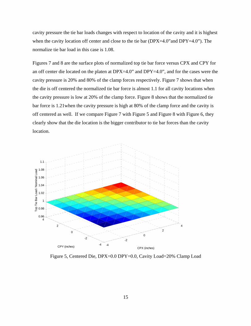
15
cavity pressure the tie bar loads changes with respect to location of the cavity and it is highest
when the cavity location off center and close to the tie bar (DPX=4.0”and DPY=4.0”). The
normalize tie bar load in this case is 1.08.
Figures 7 and 8 are the surface plots of normalized top tie bar force versus CPX and CPY for
an off center die located on the platen at DPX=4.0” and DPY=4.0”, and for the cases were the
cavity pressure is 20% and 80% of the clamp forces respectively. Figure 7 shows that when
the die is off centered the normalized tie bar force is almost 1.1 for all cavity locations when
the cavity pressure is low at 20% of the clamp force. Figure 8 shows that the normalized tie
bar force is 1.21when the cavity pressure is high at 80% of the clamp force and the cavity is
off centered as well. If we compare Figure 7 with Figure 5 and Figure 8 with Figure 6, they
clearly show that the die location is the bigger contributor to tie bar forces than the cavity
location.
Figure 5, Centered Die, DPX=0.0 DPY=0.0, Cavity Load=20% Clamp Load
-4
-2
0
2
4
-4
-2
0
2
40.96
0.98
1
1.02
1.04
1.06
1.08
1.1
CPX (inches)CPY (inches)
Top
Tie
Bar
Loa
d / N
omin
al L
oad

16
Figure 6, Centered Die, DPX=0.0 DPY=0.0, Cavity Load=80% Clamp Load
Figure 7, Off Centered Die, DPX=4.0”, DPY=4.0”, Cavity Load=20% Clamp Load
-4
-2
0
2
-4
-2
0
2
40.96
0.98
1
1.02
1.04
1.06
1.08
1.1
CPX (inches)CPY (inches)
Top
Tie
Bar
Loa
d / N
omin
al L
oad
-4
-2
0
2
-4
-2
0
2
41.05
1.1
1.15
1.2
1.25
CPX (inches)CPY (inches)
Load
on
Top
Tie
Bar
/ N
omin
al
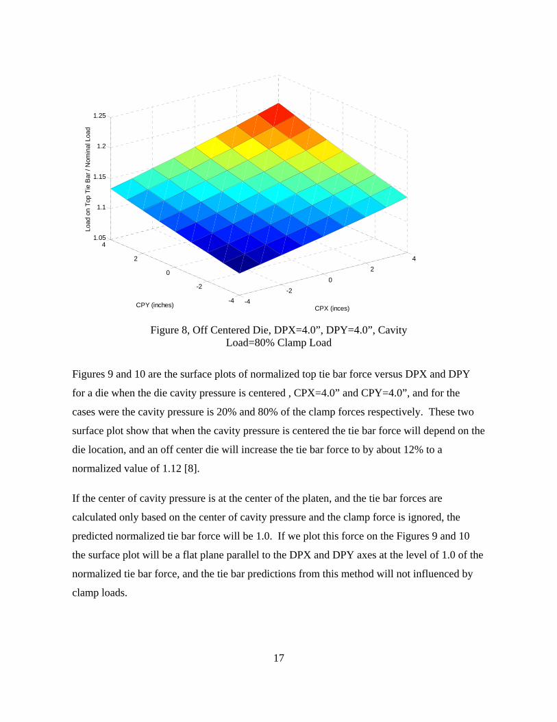
17
Figure 8, Off Centered Die, DPX=4.0”, DPY=4.0”, Cavity Load=80% Clamp Load
Figures 9 and 10 are the surface plots of normalized top tie bar force versus DPX and DPY
for a die when the die cavity pressure is centered , CPX=4.0” and CPY=4.0”, and for the
cases were the cavity pressure is 20% and 80% of the clamp forces respectively. These two
surface plot show that when the cavity pressure is centered the tie bar force will depend on the
die location, and an off center die will increase the tie bar force to by about 12% to a
normalized value of 1.12 [8].
If the center of cavity pressure is at the center of the platen, and the tie bar forces are
calculated only based on the center of cavity pressure and the clamp force is ignored, the
predicted normalized tie bar force will be 1.0. If we plot this force on the Figures 9 and 10
the surface plot will be a flat plane parallel to the DPX and DPY axes at the level of 1.0 of the
normalized tie bar force, and the tie bar predictions from this method will not influenced by
clamp loads.
-4
-2
0
2
4
-4
-2
0
2
41.05
1.1
1.15
1.2
1.25
CPX (inces)CPY (inches)
Load
on
Top
Tie
Bar
/ N
omin
al L
oad

18
Figure 9, Centered Cavity Pressure, CPX=0.0, CPY=0.0, Cavity Load=20% Clamp Load
Figure 10, Centered Cavity Pressure, CPX=0.0, CPY=0.0, Cavity Load=80% Clamp Load
-4-2
02
4
-4
-2
0
2
4
0.9
1
1.1
1.2
DPX (inches)DPY (inches)
Loa
d on
Top
Tie
Ba
r-2
/ N
omin
al L
oad
-4-2
02
4
-4
-2
0
2
4
0.9
1
1.1
1.2
DPX (inches)DPY (inches)
Lo
ad o
n T
op
Tie
Ba
r-2
/ No
min
al L
oad

19
To verify the validity of the correlations for the tie bars forces, the predictions from these
equations were compared to tie bar forces calculated from computer simulations for various
die casting machines with different tonnage and configurations and boundary conditions
between cover platen and machine base. The tonnage of these machine ranges from 250 to
3500 tons. Also the predictions from the Equations 1 and 2 were compared to experimental
measurements from a 250 ton machine [8]. All these results indicated that overall prediction
values and patterns are very satisfactory and give good results.
6. Correlation to Predict Cover Side and Ejector Side Parting
Plane Separation
Correlation to predict the parting plane separations of cover and ejector side were developed
based on computer simulation runs. The selected factors and their range are shown in Table 5
[8]. The continuous factors are Platen thickness (PT), horizontal and vertical dimension of the
die (Lx and Ly), die thickness (t), die thickness ration (TR), which is the ratio of the die
shoulder to total dir thickness, and pillar diameter (PD). X denotes the pillar pattern which is a
discrete variable. Four pillar patterns were selected for the purpose of parting plane separation
study. The units for Platen thickness horizontal and vertical dimensions of die, die thickness
and pillar diameter are in inches, the die thickness ration and pillar pattern have no
dimensions.
The design of the experiments had 58 runs, which they were repeated for each pillar patterns.
Therefore a total of 232 computer simulation runs were performed and the cover side and
ejector side separation were calculated from the results of the simulation, as described in the
previous section.
Similar to tie bar studies, non-linear power law models were selected to fit the results of the
computer simulations based on the non-dimensional parameters [13, 14, 15, 20, 8]. The non-
dimensional parameters that were derived based on PI-Theorem are shown in Table 6. The die
thickness “t” was selected as the length factor for non-dimensionalization.

20
Factor Description Low Level High Level
PT Platen thickness 9 13
Lx Horizontal dimension of the die 24 38
Ly Vertical dimension of the die 24 38
t Die thickness 5 10
TR Die thickness ratio 0.4 0.5
PD Pillar diameter 1.5 4
X Pillar Pattern (discrete factor) 4 Levels/Patterns
Table 5, Design of Experiments Factors for Parting Plane Separation
In Table 6 Lcx and Lcy are the characteristic dimensions of the cavity. And they can be
calculated from the geometry of cavity shape. Lcx and Lcy represent the bounding box of the
cavity [8]. Once one of these lengths, for example Lcx, is selected the other dimension is
calculated from the basic area relation of
A Lcx x Lcy
where A is the projected area of the cavity.
The maximum separations of the cover and ejector side are non-dimensionalized by die
thickness, Young’s Modulus and distributed contact load., which is defined as:
x y x y
Total Clamp Load Cavity Pressure Projected Area of CavityDistrubted Contact Load
L L L L
The above equation represent a uniform pressure load on the contacting surfaces of the of the
cover and ejector dies.
In Table 6, the non-dimensional parameters П1 to П6 are independent variables (inputs) and
П7 is the dependent variable (output). Ltb is the distance between the centers of the tie bars.

21
In the design of experiments Ltb was kept constant, but П1 parameter is a variable since “t”
the die thickness is changing [8].
Parameter Description
П1 (Ltb/t) or (Distance between tie bar centers/Die thickness)
П2 (Pt/t ) or (Platen thickness/Die thickness)
П3 (TR) or (Die shoulder thickness/Die thickness)
П4 (L/t ) or (Span/Die thickness)
П5 (Lcx/Lcy) or (Aspect ratio of the cavity)
П6 (Lx/Ly) or (Aspect ratio of the die)
П7 (Max Separation/t)× (Young’s Modulus/Distributed contact load)
Table 6, Non-Dimensional Parameters of Parting Plane Separation
The correlations for predicting maximum cover and ejector side separation are given by
Equation 3 and 4 [8]:
1.81.81 1.9 3.5
Max Cover Sep E Ltb PT Lx Lx Lcy0.4
t Dist load t t t Ly Lcx
(3)
3.10.95 1.5
1 np
1.53.8
1 npiavg
0.41
Max Ejector Sep E PT Ltb20.2 26.6 1
t Dist load Ltb t
LL1x L1y RWX RWY1.6
2t 2t t
Lx Lcy1
Ly Lcx
(4)
where PD is the pillar diameter, np is the number of pillars, RWX and RWY are the thickness
of the frame in X and Y directions, L1x and L1y are the longest distances between the pillars
and frame in X and Y directions, L2, L3, …., Ln are the span between the pillars , E is the
Young’s Modulus, and Liavg is the average span between the pillars given by:

22
2 3 niavg
L L ....... LL
n
(5)
Figures 11a to 11d show L1x, L1y, RWX, RWY, and Ls for the four pillar patterns used for
the design of experiments [8]. In selecting the length scales for pillars, an attempt should be
made to select the independent length scales that represents the pillar geometry and its
distribution. By introducing an average length scale for pillars, if the scales are not
independent, the averaging method, Equation 5, will compensate for dependency if any exists.
Figure 11-a, Length Scales for Pillar Pattern 1 LIavg = ((L2+L3+L4)/3

23
Figure 11-b Length Scales for Pillar Pattern 2 LIavg = 0.0
Figure 11-c Length Scales for Pillar Pattern 3 LIavg = (L2+L4)/2

24
Figure 11-d Length Scales for Pillar Pattern 4 LIavg =(L3+L4)/2
Figure 12 shows the surface plot for maximum cover separation versus die thickness and die
length for three platen thicknesses [8]. This plot shows that as platen thickness increases the
maximum separation decreases, and as the die thickness increases the maximum separation on
the cover side will increase. Figure 12 also shows that for a larger die the maximum
separation will be larger compare to a die with smaller foot print.
Figure 13 is a surface plot of maximum cover side separation versus platen thickness and die
thickness for three die lengths [8]. Figure 13 shows that as platen thickness increases and die
thickness decrease the maximum cover separation will decrease for all die sizes. And the
larger die footprints will have larger cover side separation compared to smaller die footprints
under the same conditions.
Figure 14 is a surface plot of maximum cover side separation versus die thickness and
distance between tie bars for three die lengths [8]. This plot shows that platen size has a larger
effect on reducing the cover side separation than does die thickness. A small die has smaller
cover side separation than a larger die mounted on the same size platen.

25
A careful study of equation 3 shows that the major contributors to the cover side separation
are, Die footprint or die length, Lx, platen thickness, Pt, Tie bar distance , Ltb and finally die
thickness, t [8].. The powers of their contributions are:
Die footprint, die length, Lx - power on the order of 3.
Platen thickness, PT - power on the order of -1.9.
Tie bar distance, Ltb - power on the order of -1.8.
Die thickness, “t“- power on the order of 1.2.
Figure 12, Maximum Cover Die Separation Versus Die thickness and Die Length(Ltb= 44 inches, Lx/Ly = 1, Lcx/Lcy = 0.58)
The correlation for maximum cover side separation, Equation3, and its graphical plots clearly
show that the die performs the best when it is of nominal die thickness mounted on the
thickest platen or in other words, when the ratio of die foot print to platen size is small (
around 60 percent), the cover side separation will be the smallest. If a large die is mounted on

26
a platen where this ratio is large (around 80 percent) to reduce the cover side separation a thin
die should be used. The decision about choosing size of die or size of platen also depends on
the contact stresses between the die and platen, coining (high stress, yielding) may happen if a
very small die is selected.
Figure 13, Maximum Cover Die Separation Versus Die thickness and Platen Thickness (Ltb= 44 inches, Lx/Ly = 1, Lcx/Lcy = 0.58)

27
Figure 14, Maximum Cover Die Separation Versus Die thickness and Distance between Tie Bars (Ltb= 44 inches, Lx/Ly = 1, Lcx/Lcy = 0.58)
Figure 15 is a surface plot of maximum ejector side separation versus die thickness and pillar
diameter for four pillar patterns [8]. This figure shows that the largest separation is for Pillar
Pattern 2 when there is no pillar support. Pillar Pattern 1 and 4 are the same. The vertical and
horizontal pillars in Pattern 4 provide adequate support behind the cavity to reduce the ejector
side separation. The four pillars located 45 degree from vertical or horizontal pillars do not
contribute much and give no additional support to cavity.
Figures 16 and 17 are surface plots of maximum ejector side separation versus die thickness
and die length for three platen thicknesses for Pillar Pattern 1 with Pillar diameters of 4’’ and
1.5” respectively [8]. . This plot shows that the main contributor to maximum separation on
ejector side is the die thickness. Die length and platen thickness are the next factors that
affect ejector side separation. Comparing Figure s16 and 17 it can be seen when the pillar
diameter is small a thicker platen reduces the maximum ejector side separation.

28
The largest contributor to the ejector side separation is the unsupported span behind the
ejector side. As can be seen from the pillar patterns, Figures 11-a to 11-d, and Equation 4,
the unsupported span is characterized by the numbers of pillars, size of the pillars and location
of pillars or pillar patterns. The next major contributor to maximum ejector side separation is
the die thickness and the distance between the tie bars [8]. The powers of their contributions
are:
Unsupported span, Liave, - power is on the order of 3.5
Die thickness, t, - power is on the order of -2.8
Tie bar distance, Ltb - power is on the order of -1.5
Figure 15, Maximum Ejector Die Separation Versus Die thickness and Pillar Diameter (Ltb= 44 inches, Lx/Ly = 1, Lcx/Lcy = 0.58)

29
Figure 16, Maximum Ejector Die Separation Versus Die thickness and Pillar Diameter (Ltb= 44 inches, PD=4.0 inches, Lx/Ly = 1, Lcx/Lcy = 0.58)
Figure 17, Maximum Ejector Die Separation Versus Die thickness and Pillar Diameter (Ltb= 44 inches, PD=4.0 inches, Lx/Ly = 1, Lcx/Lcy = 0.58)

30
6.1 Rules to Characterize the Spans Between Pillars and the
Spans Between Pillars and Rails
It was observed during the model adequacy study that the ejector side parting plane separation
is very sensitive to the span between the pillars and the definition of spans should be
consistent with span definitions used in the power law model development. The following
guidelines characterize the spans between the pillars and between the pillars and the rails [8].
1. The span between the pillars and the rails should be defined from the edge of the
outermost pillar and the inner edge of the rails. This is illustrated in Figure 18-a, where
the Lo’s denote the spans between the pillars and rails.
2. If a pillar is present directly behind the center of pressure, the inner spans are defined
as the horizontal and vertical distances from the edge of this center pillar to the edge
of the outer pillars as shown in Figure 18-a where the inner spans are represented by
Li’s.
3. If a pillar is not present behind the center of pressure, the inner spans Li are defined as
the horizontal and vertical distances from the center of pressure to the edge of the
outer pillars as shown in Figure 18-c.
4. If only one pillar is present then the outer spans Lo are defined between the outer edge
of the pillar to the inner edge of the rails and the inner spans Li are defined from the
center of pressure to the outer edge of the pillar. This is illustrated in Figure18-d.
The rules summarized above can be used as a guideline to characterize the spans between the
pillars and the rail supports to be used in the power law model to predict the ejector side
separation
It should be reiterated that since we are using an average span for the pillars, this average
process will correct for small inconsistencies such as more spans are defined of if these spans
are not independent or they are not exactly defined according to above rules.

31
Figure 18, Sketches for Characterizing the Spans behind the Ejector Die
7. Equivalent Machine Stiffness
The above correlation model was developed based on the die and die casting machine model
described in Section 2. As can be seen from Figure 1, in this machine model platens are
represented by a rectangular shape with a constant thickness [8]. In actual die casting
machines platens can have ribs; grooves, cuts and the thickness are not usually constant along
the vertical direction of platens. Even some cast platens have thick ribs to give more support
and to reduce the mass of platens. For these types of machines an equivalent platen with
constant thickness which has the same stiffness as the actual platen should be used in the
above correlations for each platen.
The locations and arrangements of toggle mechanism behind the ejector platen is different for
various die casting machine. Two platens which have the same thickness but different toggle
locations or patterns, such as four pad location versus two pad locations, could have different

32
stiffness characteristics due to the differences in force location, moments from these forces
and ejector geometry. Therefore this should be conceded when one wants to used the
correlations. The correlations are developed based on the die casting machine model shown
on Figure 1, this model has four pad or locations where toggle mechanism exerts forces on the
ejector platen [8].
Platens provide supports for the dies. Their main task is to prevent deflection along the tie bar
direction, and reduce the parting plane separation to a minimum. Therefore the equivalent
stiffness that is relevant is the deflection along the tie bars or in our cases along the Z-
directions. Therefore the equivalent platen can be determined by comparing the displacement
of the actual platen to equivalent platen.
The relation between the load, deflection and stiffness is given by
F K x
where F is the force, K is the stiffness and ∆x is the deflection.
Finding the equivalent platen thickness uses a series of static finite element analyses to obtain
the force and deflection data for both the actual and equivalent platens. The deflections of the
actual platen under different magnitudes of force are calculated from analyses. Also a series
analyses are done with a solid rectangular platen with various thicknesses. It is important that
the loads be applied at the same locations where dies are attached to the platens in the
analyses runs. These loads are applied as boundary conditions for both actual and equivalent
platens. The constraints used in these models are different for the cover and ejector platens.
Figures 19 and 20 show a four toggle location platen with ribs design [8]. This sample platen
will be used to show the steps and procedures to calculated equivalent cover and ejector
platens. The equivalent cover or ejector platen thickness can be used in the above
correlations.
7.1 Steps to Determine Equivalent Cover Platen Thickness
The cover platen is attached/ bolted to the machine tie bars and the bottom of the cover platen
is bolted or welded to the machine base. One end of the tie bar attached to the cover platen
33
and the other ends of the tie bars are secured to the rear platen. In the proposed method the tie
bars are modeled explicitly and one end of the tie bars is attached to the platen using a tied
contact. The nodes on the other end of the tie bar are constrained in space in all directions.
The bottom of the platen is constrained in all directions. Figure 20 shows the finite element
model with the constraints on the bottom of platen and on the tie bars. A uniform load is
distributed on the platen center over an area equal to the die mounted on the machine; in this
case this area is 31” by 31”. This loading area and its location can be changed depending on
the size of the die and where it is mounted in the actual machine. Four load magnitude are run
for each case. In this example loads are 250 tons, 500 tons, 750 tons and 1000 tons [8].
The maximum deflection of the ribbed platen is calculated for each of the loading cases. For
platen stiffness calculations only the platen deflection is important.
The analyses will give total deflection at each location on the platen; from this total deflection
the tie bar deflection or stretching should be removed to calculate only the platen deflections.
Then the deflections of solid rectangular platens with thicknesses of 0.2795 meters (9 inches),
0.254 meters (10 inches) and 0.2286 meters (11 inches) are also obtained from analyses runs.
The deflection values for the solid platens are obtained at a location which is same as the
location of maximum deflection on the actual platen.
The load deflection curves for the actual platen, and solid rectangular platens with thickness
of 0.2795 meters (9 inches), 0.254 meters (10 inches) and 0.2286 meters (11 inches) are
shown in Figure 21 [9]. As can be seen from these figure a solid rectangular 9 inch platen has
the same stiffness as the actual platen shown in Figures 18 and 19. Therefore a nine inch solid
rectangular platen can represent the ribbed cover platen in the above correlations

34
Figure 19, Selected Platen Design for Equivalent Stiffness Study
Figure 19, Dimensions of the Selected Platen Design for Equivalent Stiffness Study (Dimensions in Inches)

35
Figure 20, Finite Element Model Used to Determine the Cover Platen Stiffness
Figure 21, Deflection versus Forces Curves for Cover Platen
Deflection Vs Load y_9" = 4551731632.71x - 6.83y_rib = 4470805440.54x - 17.88
y_10" = 5318714310.27x - 5.32y_11" = 6047360126.79x + 9.07
0
1000000
2000000
3000000
4000000
5000000
6000000
7000000
8000000
9000000
10000000
0 0.0005 0.001 0.0015 0.002 0.0025
Deflection (meters)
Lo
ad
(N
ew
ton
)
Ribbed
Solid-9"
Solid-10"
Solid-11"
36
7.2 Steps to Determine Equivalent Ejector Platen Thickness
The steps to determine the equivalent solid rectangular ejector platen stiffness to be used in
the above correlation from an actual ejector platen design are basically similar to the cover
platen procedures. The differences are the way the platen forces and constraints are imposed
on the mesh models. The ejector platen can freely slide on the tie bars and the toggle
mechanism transmits the clamp loads on the ejector platen and can add some stiffness to the
ejector platen. Therefore the toggles mechanism model should be included in the ejector
platen model to predict the ejector platen stiffness. The toggle mechanism is modeled as three
dimensional equivalent beam elements in the finite element models. One end of these beams
attached to the ejector platen and the other end of the beams are constrained in space in all
degrees of freedom for both the actual ejector platen and its equivalent solid rectangular
platen. Figure 22 shows the finite element model of the actual ribbed platen with the
constraints [8].
The forces or loads are applied on the area where the dies are mounted on the platen for both
the actual ejector platen and for the solid rectangular platen. For this example, loads are
uniformly distributed over an area of 31” by 31” on the center of the platens. Four load cases
are run. In this case the loads are of 250 tons, 500 tons, 750 tons and 1000 tons. A series of
static analyses runs were performed on the platens and the maximum deflection of the actual
ribbed platen and solid rectangular platens with different thickness were obtained from
analyses runs. The deflection of the equivalent platen is obtained at the location were the
deflection is the highest for the actual platen design.
The force versus deflection curves for actual platen design and solid rectangular platens with
thickness of 0.2795 meters (9 inches) and 0.254 meters (10 inches) are shown in Figure 23
[8]. This figure shows that a solid rectangular 9 inch platen exhibits the same stiffness
characteristic as the actual ribbed ejector platen.

37
Figure 22, Finite Element Model Used to Determine the Ejector Platen Stiffness
Figure 23, Deflection versus Load Curves for Ejector Platens
Deflection Vs Load y_rib = 3578847885.62418x y_9" = 2852503674.45180x + 2.8y_10" = 3793433298.8133x
0
1000000
2000000
3000000
4000000
5000000
6000000
7000000
8000000
9000000
10000000
0 0.0005 0.001 0.0015 0.002 0.0025 0.003 0.0035
Deflection (meters)
Lo
ad
(N
ew
ton
)
Ribbed
Solid-9"
Solid-10"

38
7.3 Steps to Determine Equivalent Ejector Platen Thicknesses
with Different Toggle Locations
The toggle mechanism is attached to ejector platen at one side and to rear platen at the other
side. The toggle mechanism attachment to ejector platen varies from one machine to another.
The way toggle mechanism is attached to ejector platen should be addressed because the
location and number of pads/attachments will affect the stiffness of the ejector platen. For
example a machine with two toggle ejector platen has a different stiffness than a machine with
four toggle platen. Since the above correlation are determined from a two toggle machine
platen, if these correlations are used to predict the parting plane separation for a four toggle
machine the equivalent ( two toggle thickness) ejector platen should be in the correlations.
Figure 24 shows the mesh models for decrementing thickness of a two toggle ejector
mechanism for a four toggle ejector platen [8]. Figure 24-A and Figure 24-B show models of
tow toggle and four toggle location machines. The toggles are modeled using three dimension
beams, each beam have the same stiffness as the actual toggle mechanism.
A B
Fire 24, Models Used to determine the Equivalent Stiffness of Four Toggle
The other ends of the beans are constrained in all directions. In our example, the maximum
deflections at the same location are calculated using a static analysis for of the two toggle

39
platen and four toggle platens. The forces were 250 tons, 500 tons, 750 tons and 1000 tons.
These forces were distributed uniformly on the area and location where dies are mounted on
the platen; in this case the area representing the foot print of the dies was 31” by 31” inches.
Analyses should be repeated for different thicknesses of platens in order to find the equivalent
thickness.
In our example the 0.254 meters (10 inch) two toggle platen is the base line for comparison.
The above analyses steps are repeated for 0.254 meters (10 inch) two toggle platen and for
four toggle platens with 0.2286 meters (9 inches) and 0.2032 meters (8 inches). Force
deflection plots for these models are shown in Figure 25 [8].
Figure 25, Force Deflection for Two Toggle and Four Toggle Platens
As can be seen from this figure the stiffness of a 0.2032 meters (8 inches) four toggle ejector
platen is almost equivalent to a 0.254 meters (10 inches) two toggle ejector platen.
Deflection vs Loady_8"_4TG = 10950266433.03x - 164.25
y_9"_4TG = 15348952508.01x - 222.54
y_10"_2TG = 11874368631.68x - 89.05
0
1000000
2000000
3000000
4000000
5000000
6000000
7000000
8000000
9000000
10000000
0.0000 0.0002 0.0004 0.0006 0.0008 0.0010
Deflection (meters)
Lo
ad
(N
ew
ton
)
2-Toggle-10"
4-Toggle-9"
4-Toggle-8"
40
8. References
[1] Tewari, A., 2000, "Study of the Effect of Structural Variables of Die and Die Casting Machine on Die Deflections," Master’s Thesis, The Ohio State University.
[2] Ahuett-Garza, H., 1996, "Characterization of Loads in Die Casting and Prediction of Die Deflections," PhD Dissertation, The Ohio State University.
[3] Miller, R.A., 2003, "Die Deflection Modeling: Empirical Validation and Tech Transfer," US Department of Energy Project Report, Project DE-FC07-97ID13576
[4] Ahuett-Garza, H., and Miller, R. A., 2003, "The Effects of Heat Released during Fill on the Deflections of Die Casting Dies," Journal of Materials Processing Technology, 142(3) pp. 648-658.
[5] Ragab, A , 2003, , "Sensitivity Analysis of Casting Distortion And residual Stress Prediction through Simulation Modeling And Experimental Verification," PhD Dissertation, The Ohio State University.
[6] Arrambide, E., 2004, "Modeling Influence of The Die Casting Machine Components on Contact Pressure between Dies and Platens," Master’s Thesis, The Ohio State University.
[7] Xue, H., Kabiri-Bamoradian, K., and Miller, R. A., 2005, "Modeling the dynamic cavity pressure and impact spike in die casting," NADCA Transactions.
[8], Murugesan, K. S., 2008, , "Predicting Parting Plane Separation And Tie Bar Loads in Die casting Using Computer Modeling and Dimensional Analysis ," PhD Dissertation, The Ohio State University.
[9] Ragab, A., Kabiri-Bamoradian, K., and Miller, R. A., 2001, "Modeling part distortion and stresses in die casting," NADCA Transactions, pp. 77-83.
[10] Ragab, A., Kabiri-Bamoradian, K., and Miller, R. A., 2004, "Part distortion and stress prediction in die casting process: Sensitivity analysis," NADCA Transactions.
[11] Garza-Delgado, A., Kabiri-Bamoradian, K., and Miller, R. A., 2007, "Finite element modeling of casting distortion in die casting," NADCA transactions.
[12] Garza-Delgado, A, 2007, “A Study of Casting Distortion And Residual Stress in Die Casting , “PhD Dissertation, The Ohio State University.
[13] Buckingham, E., 1914, "On Physically Similar Systems; Illustrations of the use of Dimensional Equations," Physical Review, IV(4) pp. 345-376
[14] Buckingham, E., 1915, "Model Experiments And The Forms of Empirical Equations," Transaction of American Society of Mechanical Engineers, pp. 263-297

41
[15] Vignaux, G. A. And Scott J. L., 2001, “Simplifying Regression Models Using Dimensional Analysis,” Research Publication in Australian and New Zeeland Journal of Statistics.
[16] Arrambide, E., Ragab, A., Kabiri-Bamoradian, K., Miller, R. A., 2005 “Modeling Influence of the Die Casting Machine Components on Contact Load Between Dies and Platens”, Proceeding CastExpo’05 Congress 2005, St. Louis, Missouri, April 16-19, 2005.
[17] Murugesan, K. S., Ragab, A., Kabiri-Bamoradian, K., Miller, R. A., 2005 “Effect of Die, Cavity and Toggle Locations on the Tie Bar Forces, Toggle Forces Parting Plane Separation,” Proceeding of CastExpo’05 Congress 2005, St. Louis, Missouri, April 16-19.
[18] Murugesan, K. S., Ragab, A., Kabiri-Bamoradian, K.,Miller, R. A., 2006, “A Model to Predict Tie Bar Load Imbalance,” Proceeding CastExpo’06 Congress , Columbus, OH, April 18-21.
[19] Murugesan, K. S., Ragab, A., Kabiri-Bamoradian, K., Miller, R. A., 2007 “An Experimental Verification of the Effect of Die Location on the Tie Bar Load Imbalance,” Proceeding of 111th MetalCasting Congress, Houston TX, May 15-18.
[20] Murugesan, K. S., Kabiri-Bamoradian, K., Miller, R. A., 2008, “The Effect of Support Pillar Patterns on the Mechanical Performance of the Ejector Side Dies,” Proceeding of CastExpo’08 Congress, Atlanta, GA, May 17-20.
[21] Kinatingal, J. X., 2005, "Study of The Effect of Structural Die and Machine Variables on Die Deflections," Master’s Thesis, The Ohio State University.

Appendix B: Door Closer Die Case Study

DoorCloserDieCaseStudy
Adham Ragab Khalil Kabiri-Bamoradian
OSU Center for Die Casting
May 2004

Door Closer Case Study 2
Background The die used for the housing of a door closing mechanism suffered premature cracks on the ejector die cavity surface. These cracks led to marks on the casting surface that were visible when the casting is in use making the casting unacceptable. The onset of the cracks in the ejector die was at approximately 20,000 – 40,000 shots, much below the design expectation. This problem led to unexpected cost elevation. Several techniques were tried by the die caster to fix the problem, but with no success. Since the cause of the problem was thought to be flexing of the die, the Center for Die Casting at Ohio State University was asked to analyze the die using die distortion modeling techniques developed over the past several years. Figures 1 and 2 show the casting and the marks on its outer surface respectively. Several modifications were made to the casting and the ejector insert to avoid the crack formation with little success. The modifications included changes in the casting geometry and adding cooling lines to the ejector insert. The last modification was to split the ejector insert into two pieces to minimize the bending strains. This problem was to simulate the die and the casting process using the techniques developed in the Center for Die Casting at the Ohio State University in order to investigate the reason for the cracks and to propose some modifications to minimize it. Computer Simulation Model One of the problems faced in building this model was that the solid model that we had for the casting and inserts was not adequate for meshing. The solid model suffered from gaps and overlapped surfaces in many locations, especially at the interactions between fillets.
Figure 1 The casting Figure 2: Casting defects

Door Closer Case Study 3
These gaps and overlaps were too severe to be fixed and a new solid model was built from scratch. Another problem was the computational resources needed for running the model. Since the problem studied was basically on the cavity surface, the mesh had to depict the surface details as thoroughly as possible. This led to a large model that could not be run on a PC. Running the model on the Ohio Super Computer did not produce much improvement. Although the super computer could run this big model, it was too slow (in clock time, not CPU cycle time) to be practical. To overcome this problem, the casting geometry and hence the insert geometry was simplified to decrease the required model size. The simplifications were made as far as possible from the crack areas which was the main concern in this analysis. A sequentially coupled thermo-mechanical finite element analysis was conducted to simulate the casting process. This type of analysis is divided into two stages: a thermal stage and a structural stage. In the first stage a pure thermal analysis was run for fifteen casting cycles. The goal is to allow the die temperature to reach a quasi-steady state. The cycle time was given as shown in Table1.
Cycle Segment Time (Sec) Metal injection 0.04 Solidification 29.96 Die opening 2.0 Slide retraction 3.0 Part ejection 5.0 Spraying 6.0 Idle 9.0 Die closing 2.0 Total cycle time 57.0
Table 1: Cycle time
The thermal analysis includes the casting, inserts, dies and slides. Cooling lines are active in the model with a heat transfer coefficient of 3000 W/m2K to a constant temperature coolant of 20oC. The ambient temperature is assumed constant at 30oC. The heat transfer coefficient from the dies to the environment is 20 W/m2K. Heat transfer between the casting and the inserts is assumed constant at 3000 W/m2K. The heat transfer coefficients between insert/insert, insert/die, die/die and slide/insert are constant at 1000 W/m2K. The initial temperature of the molten metal is 650oC. In the structural stage of the analysis, only the inserts and dies are included due to the model size constraints on a PC. Figure 3 shows the solid model of the die set. The finite element model was created using 10-noded quadratic tetrahedron elements. Figure 4 shows the element with its nodes and integration points [ABAQUS, 1998]. While this type of elements is reliable in structural analysis, its thermal results are not accurate. This problem is defined in ABAQUS manual as “Spurious oscillations due to small time

Door Closer Case Study 4
increments”. To overcome this problem the middle nodes in the 10-noded element are removed in the thermal analysis and the element is used as a 4-noded linear tetrahedron element. When reading the temperature distribution from the thermal results file into the structural analysis, the temperature of the middle nodes are linearly interpolated from the temperature of the element corner nodes. A clamping load of 5000 KN was applied as a pressure boundary condition on the back of the ejector die. The intensification pressure was applied on the cavity surface with a value of 70 MPa (10,000 psi.). The structural analysis consists of three steps. In the first step the clamping load is applied. In the second step the intensification pressure is added. In the third step the temperature distribution from the thermal analysis results is input to the structural analysis. Results from each step are saved in the structural results file. Another structural analysis was run with the third step only to investigate the effect of thermal load without interaction or interference with mechanical loads. Results and Discussion Figures 5 and 6 show the locations of the main cracks relative to the casting and insert respectively. Figures 7 and 8 show the equivalent strain in the ejector insert due to thermal loads and mechanical loads respectively. Figures 9 and 10 show the equivalent strain due to thermal loads and mechanical loads respectively, at the crack locations. Figure 11 shows the equivalent strain due to thermo-mechanical loads at the crack locations. The equivalent strain, shown in Figures 6-11, was calculated using equation (1).
Figure 3: Die set model Figure 4: 10-noded tetrahedron element
(1) )()()(23
1 232
231
221 e

Door Closer Case Study 5
Where: εe= Equivalent strain ε1= Max. principal strain ε2= Mid. principal strain ε3= Min. principal strain
Figure 7: Equivalent strain in the ejector insert due to thermal load only. (Dark blue= 0.0000 – 0.00042, Red = 0.00458 – 0.005, light green = 0.00167 – 0.00208)
Figure 5: Main crack locations with respect to the casting
Figure 6: Main crack locations with respect to the ejector insert
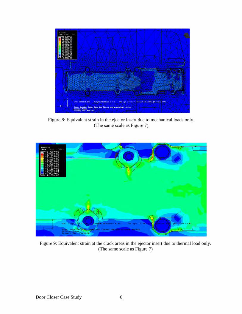
Door Closer Case Study 6
Figure 8: Equivalent strain in the ejector insert due to mechanical loads only. (The same scale as Figure 7)
Figure 9: Equivalent strain at the crack areas in the ejector insert due to thermal load only. (The same scale as Figure 7)

Door Closer Case Study 7
Figure 10: Equivalent strain at the crack areas in the ejector insert due to mechanical loads only. (The same scale as Figure 7)
Figure 11: Equivalent strain at the crack areas in the ejector insert due to thermo-mechanical loads. (The same scale as Figure 7)
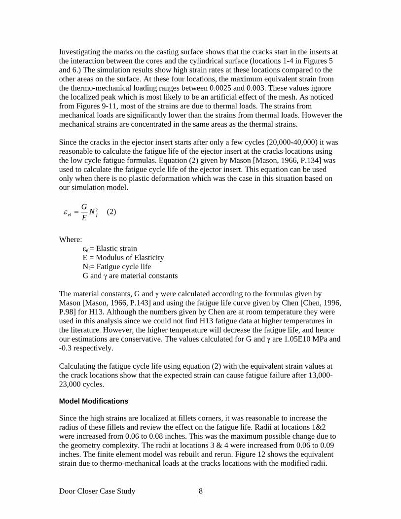
Door Closer Case Study 8
Investigating the marks on the casting surface shows that the cracks start in the inserts at the interaction between the cores and the cylindrical surface (locations 1-4 in Figures 5 and 6.) The simulation results show high strain rates at these locations compared to the other areas on the surface. At these four locations, the maximum equivalent strain from the thermo-mechanical loading ranges between 0.0025 and 0.003. These values ignore the localized peak which is most likely to be an artificial effect of the mesh. As noticed from Figures 9-11, most of the strains are due to thermal loads. The strains from mechanical loads are significantly lower than the strains from thermal loads. However the mechanical strains are concentrated in the same areas as the thermal strains. Since the cracks in the ejector insert starts after only a few cycles (20,000-40,000) it was reasonable to calculate the fatigue life of the ejector insert at the cracks locations using the low cycle fatigue formulas. Equation (2) given by Mason [Mason, 1966, P.134] was used to calculate the fatigue cycle life of the ejector insert. This equation can be used only when there is no plastic deformation which was the case in this situation based on our simulation model. Where: εel= Elastic strain E = Modulus of Elasticity Nf= Fatigue cycle life G and γ are material constants The material constants, G and γ were calculated according to the formulas given by Mason [Mason, 1966, P.143] and using the fatigue life curve given by Chen [Chen, 1996, P.98] for H13. Although the numbers given by Chen are at room temperature they were used in this analysis since we could not find H13 fatigue data at higher temperatures in the literature. However, the higher temperature will decrease the fatigue life, and hence our estimations are conservative. The values calculated for G and γ are 1.05E10 MPa and -0.3 respectively. Calculating the fatigue cycle life using equation (2) with the equivalent strain values at the crack locations show that the expected strain can cause fatigue failure after 13,000-23,000 cycles. Model Modifications Since the high strains are localized at fillets corners, it was reasonable to increase the radius of these fillets and review the effect on the fatigue life. Radii at locations 1&2 were increased from 0.06 to 0.08 inches. This was the maximum possible change due to the geometry complexity. The radii at locations 3 & 4 were increased from 0.06 to 0.09 inches. The finite element model was rebuilt and rerun. Figure 12 shows the equivalent strain due to thermo-mechanical loads at the cracks locations with the modified radii.
(2) fel NE
G

Door Closer Case Study 9
Figure 12 shows that the equivalent strains range between 0.0019 and 0.003. Calculating the fatigue life using equation (2), it yields that the fatigue life would range between 13,000 and 60,000 cycles. The main improvement in fatigue life took place in locations 3 & 4. At these two locations, the expected fatigue life increased from 23,000 to 60,000 cycles. Locations 1 & 2 did not show a significant change. It is expected to have better results at locations 1 & 2 using bigger radius than 0.08 inches which was not possible in the solid model, but can be done if the casting design changes slightly. Conclusions A case study of a die deformation was conducted. In this case the ejector insert suffered from cracks on the cavity surface after 20,000-40,000 cycles. A finite element simulation model was built to simulate the casting process and to find out the expected reason for the cracks formation. A sequentially coupled thermo-mechanical analysis was conducted and the model predicted strains were used to calculate the fatigue cycle life in the ejector insert cavity surface. The results showed that the model predicted strains can cause fatigue failure within 13,000-23,000 cycles at the cracks locations. The model results match the actual die failure pattern very well. However, the simulation predictions suggest failure somewhat earlier than has been observed. This may be due to the lack of two features in the structural model, namely, the casting and the slides. The interaction between the inserts and both the casting and slides can change the strain pattern and decrease, to some
Figure 12: Equivalent strain at the crack areas in the ejector insert due to thermo-mechanical loads: with a modified radii casting.
(The same scale as Figure 7)

Door Closer Case Study 10
extent, the tensile strains resulting from the thermal loads. Including the casting and slides in the structural model was not possible due to the need to keep computational resources manageable. The results show that the high strains are localized to a few locations. This suggests that modifying the die structure does not solve the problem. Instead changing the geometry at the crack locations can make a difference. The analysis was rerun again with modified fillet radii at cracks locations and the results showed much better results at two of the four locations. References ABAQUS Corporate, ABAQUS Standard Manual, USA (1998). Chen, C.S., ”The Effect of Pulsed Electromechanical Machining on the Fatigue Life of H-13 Steel”, Master Thesis, The Ohio State University, 1996. Mason, S.S., Thermal Stress and Low Cycle Fatigue, McGraw-Hill, New York, 1966.

Appendix C: Finite Element Modeling of Casting Distortion in Die
Casting

This paper is subject to revision. Statements and opinions advanced in this paper or during presentation are the author’s and are his/her responsibility, not the Association’s. The paper has been edited by NADCA for uniform styling and format. For permission to publish this paper in full or in part, contact NADCA, 241 Holbrook, Wheeling, Illinois, 60090, and the author.
Finite Element Modeling of Casting Distortion in Die Casting
R. Allen Miller K. Kabiri-Bamoradian
Ohio State University, Columbus, Ohio
A. Garza Simulia Erie Region, Cleveland, Ohio
ABSTRACT The finite element method has become a widely used tool in the design of a variety of mechanical, thermal or fluid systems. In the casting industry, finite element and other related computational analyses have become a common tool among the successful die casters, allowing prediction of filling patterns, thermal profiles in tooling and products, tool and machine components deflections, etc. Recently, theses analyses have been used to predict the final part shape and residual stresses in castings. Because of the complexity of the many interrelated physical phenomena taking place during the casting cycle, all of the current approaches rely on the use of assumptions to make the problem solvable. The fidelity of the computer model predictions is strictly related to the adequacy of the assumptions; thus, care should be exercised when interpreting the results. In this paper an extension to standard modeling approaches that was developed to predict final deformations and residual stresses in die castings is presented. The modeling methodology incorporates the die and machine components into the analysis and treats them as deformable bodies, enabling an accounting for the elastic deflections experienced by the tooling during operation. The elastic deflections in the cavity are tracked by using a shell mesh, the displacements of which are subsequently used to modify the casting initial surface shape prior to the onset of cooling. Furthermore, the model incorporates realistic temperature and strain rate dependent material properties to represent the casting material. The analysis is carried out as a fully-coupled thermal-mechanical model using the commercially available software ABAQUS. The casting under study is a ribbed plate used extensively in previous case studies. The FEA model of machine was patterned after a Buhler SC-250 cold chamber die casting machine available at Ohio State. Computer model deformation predictions are validated against experimental measurements taken on actual castings. The comparisons are made using the results of a set of designed experiments in which the effects of intensification pressure and dwell time were studied. The obtained results showed relatively good agreement for the selected dimensions and also raise a number of interesting questions about the ability to predict small distortions. Discussion of the results and needed additional work is presented. INTRODUCTION Casting distortion arises primarily from two main sources, uneven cooling of the different sections of the casting due to variation in geometry, and the constraint imposed by the die walls that limits the ability of the casting to shrink freely. Distortions may also be induced by die manufacturing inaccuracies, die setup errors and post-processing operations such as fixturing, machining, and quenching.
Karvi [1] identified the two primary sources of dimensional variability as: random variability in process conditions and incorrect die dimensions. Typical sources of random variability in die casting can be attributed to: variations in cycle time, injection pressure, injection velocity, metal temperature, spraying patterns, cooling line conditions, etc. All these factors have an effect on the repeatability of the process. Incorrect die dimensions and improper setup represent systematic sources of error leading to the production of castings with dimensions that are consistently off target regardless of any variability in the process conditions. The systematic nature of this source of error is usually attributed to the incorrect over sizing of the die cavity. Because metals experience shrinkage when they cool down, die cavities are usually oversized to compensate for this phenomenon. Thus, die cavities are usually enlarged by a shrinkage factor. For simplicity tool builders typically apply this factor uniformly throughout the cavity shape, inherently assuming that the casting will cool down evenly. However,

because of the irregular shapes usually encounter in die castings, cooling does not progress uniformly and some sections of the casting cool faster than others and this may result in casting distortion and dimensional inaccuracy.
Another factor that poses a major challenge in properly sizing the die cavity is the distortion the die cavity experiences due to the operating conditions. The causes and effects of die distortion in die casting have been identified by Ahuett [2]. This research work and others that followed have supported the claim that, as a result of the combined effect of mechanical and thermal loads, dies elastically deflect and their operating dimensions are somewhat different from the ones intended by the tool builder.
The restrained cooling the casting experiences while cooling inside the die leads to thermal strains. At high temperatures, the casting material yields easily and the thermal strains result in plastic deformation. However, when the material has cooled down enough to no longer yield, the thermal strains lead to elastic residual stresses, which at the point of ejection may have an effect on the way the casting distorts while cooling to room temperature. Elastic residual stresses may also be caused as a result of thermal strains generated while the casting cools outside the die due to uneven cooling of different sections.
This research focused on the development of computer modeling techniques to simulate the die casting process in order to predict the final dimensions and residual stresses in a die casting. Experimental validation of the computer model predictions of dimensions are a main objective. The results of this investigation provide insight into how process and tool design related factors affect the final deformation and residual stresses in a die casting.
Among many other things, computer model predictions rely heavily upon the representation of the system being analyzed as well the use of appropriate constitutive models and physical properties that describe the physical/mechanical behavior of the components involved. An important side objective of this research work was the determination of key high temperature mechanical properties of the die casting alloy employed in the model. The availability and use of these properties was important in order to have confidence in the predictions. The measurement of high temperature properties of the A380 alloy was reported in the 2008 transactions [3]
DIE DISTORTION MODELING Modeling of die distortion has been an active research area at the Center for Die Casting at The Ohio State University and throughout the industry. Among the contributions are [4-6] and the series of papers [7-15].
Earlier work determined that the main causes of the elastic deflections experienced by the die are: the clamping force developed by tie bar stretching, the uneven thermal profile of the die that results from the non-uniform part geometries and a quasi-steady state process that injects hot material into the same die cycle after cycle, and the intensification pressure applied to increase material feeding and reduce pore size across the casting volume. The interaction of these static loads leads to uneven elastic deflections of the die that affect the cavity dimensions.
Modeling of die distortion requires the inclusion of the die and machine elements. In this research the model was built based on a Buhler SC-250 ton cold chamber die casting machine available at Ohio State. The model included the die, ejector support block, plus the ejector and cover platens. Tie bars were not included due to the procedure used to model the clamping force which is described later. Figure 1 shows the basic model.
Because of the side to side symmetry of the machine and the casting, only half of the model was used. A symmetric boundary condition was specified on all the nodes lying at the symmetry plane, constraining their motion in the direction normal to that plane. In order to simulate the attachment of the cover platen to the machine foundation and of the contact of the ejector platen on the rails, the motion in the vertical direction of some nodes on these surfaces was restrained. The contact interaction among all the structural elements was specified as small sliding, having a coulomb friction coefficient of 0.1.
CLAMPING FORCE MODELING The effects of clamping force was modeled with a pressure load was applied on both platens as shown in Figure 2. Pressure was applied at the toggle pads on the back of the ejector platen and at the regions where the reaction from the tie bar locking nuts is developed on the cover platen as shown in Figure 3. The application of both pressure loads was done during the same simulation step. The clamping force magnitude was equally divided between the top and bottom regions on each side of the machine. Any unbalance due to die location was not accounted for. The unbalanced between the top and bottom tie bars has been estimated to be about 8%, and represents a contribution to part distortion not addressed in this model [15].
This procedure was used to arrest an observed semi-rigid body motion that resulted from tie bar stretching when tie bars were included in preliminary models. The observed motion caused divergence when contact was being established between the casting and the cavity surfaces. A more detailed description of this situation will be provided when the procedure to model the cooling of the casting inside the die is described in a later section. The assumption of equal load between the top and the bottom might result in incorrect platen distortion patterns and die sealing patterns at the parting plane. In reality, when the die is moved down the bottom tie bars take up more load and greater contact pressure magnitudes are obtained at the bottom of the parting plane. The assumption of equal load therefore, may be expected to alter this profile, possibly affecting parting

plane separation when the pressure load is applied. Additionally, tie bar load redistribution due to the effects of intensification pressure cannot be accounted for, since the pressure magnitude is kept constant throughout the analysis. The inability to account for this load redistribution may also lead to slightly different platen distortion patterns
Figure 1 Machine finite element model
Figure 2 Schematic of clamping method
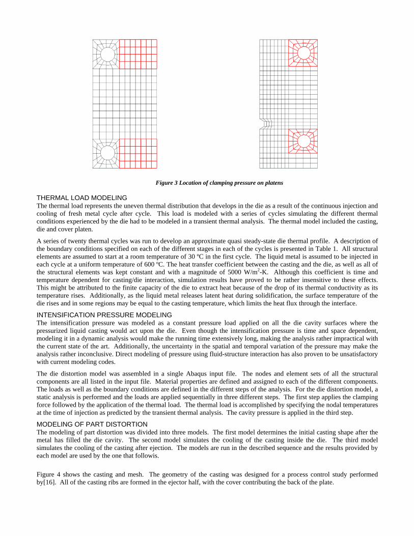
Figure 3 Location of clamping pressure on platens THERMAL LOAD MODELING The thermal load represents the uneven thermal distribution that develops in the die as a result of the continuous injection and cooling of fresh metal cycle after cycle. This load is modeled with a series of cycles simulating the different thermal conditions experienced by the die had to be modeled in a transient thermal analysis. The thermal model included the casting, die and cover platen.
A series of twenty thermal cycles was run to develop an approximate quasi steady-state die thermal profile. A description of the boundary conditions specified on each of the different stages in each of the cycles is presented in Table 1. All structural elements are assumed to start at a room temperature of 30 ºC in the first cycle. The liquid metal is assumed to be injected in each cycle at a uniform temperature of 600 ºC. The heat transfer coefficient between the casting and the die, as well as all of the structural elements was kept constant and with a magnitude of 5000 W/m2-K. Although this coefficient is time and temperature dependent for casting/die interaction, simulation results have proved to be rather insensitive to these effects. This might be attributed to the finite capacity of the die to extract heat because of the drop of its thermal conductivity as its temperature rises. Additionally, as the liquid metal releases latent heat during solidification, the surface temperature of the die rises and in some regions may be equal to the casting temperature, which limits the heat flux through the interface.
INTENSIFICATION PRESSURE MODELING The intensification pressure was modeled as a constant pressure load applied on all the die cavity surfaces where the pressurized liquid casting would act upon the die. Even though the intensification pressure is time and space dependent, modeling it in a dynamic analysis would make the running time extensively long, making the analysis rather impractical with the current state of the art. Additionally, the uncertainty in the spatial and temporal variation of the pressure may make the analysis rather inconclusive. Direct modeling of pressure using fluid-structure interaction has also proven to be unsatisfactory with current modeling codes.
The die distortion model was assembled in a single Abaqus input file. The nodes and element sets of all the structural components are all listed in the input file. Material properties are defined and assigned to each of the different components. The loads as well as the boundary conditions are defined in the different steps of the analysis. For the die distortion model, a static analysis is performed and the loads are applied sequentially in three different steps. The first step applies the clamping force followed by the application of the thermal load. The thermal load is accomplished by specifying the nodal temperatures at the time of injection as predicted by the transient thermal analysis. The cavity pressure is applied in the third step.
MODELING OF PART DISTORTION The modeling of part distortion was divided into three models. The first model determines the initial casting shape after the metal has filled the die cavity. The second model simulates the cooling of the casting inside the die. The third model simulates the cooling of the casting after ejection. The models are run in the described sequence and the results provided by each model are used by the one that followis.
Figure 4 shows the casting and mesh. The geometry of the casting was designed for a process control study performed by[16]. All of the casting ribs are formed in the ejector half, with the cover contributing the back of the plate.
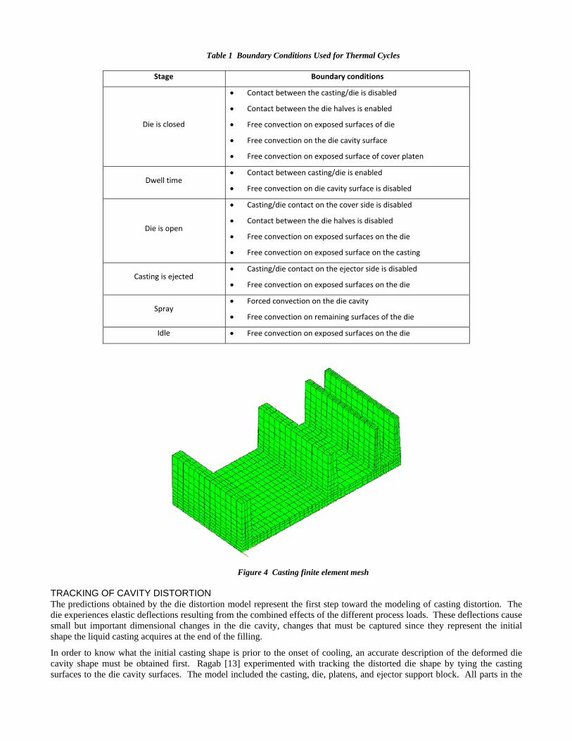
Table 1 Boundary Conditions Used for Thermal Cycles
Stage Boundary conditions
Die is closed
Contact between the casting/die is disabled
Contact between the die halves is enabled
Free convection on exposed surfaces of die
Free convection on the die cavity surface
Free convection on exposed surface of cover platen
Dwell time Contact between casting/die is enabled
Free convection on die cavity surface is disabled
Die is open
Casting/die contact on the cover side is disabled
Contact between the die halves is disabled
Free convection on exposed surfaces on the die
Free convection on exposed surface on the casting
Casting is ejected Casting/die contact on the ejector side is disabled
Free convection on exposed surfaces on the die
Spray Forced convection on the die cavity
Free convection on remaining surfaces of the die
Idle Free convection on exposed surfaces on the die
Figure 4 Casting finite element mesh TRACKING OF CAVITY DISTORTION The predictions obtained by the die distortion model represent the first step toward the modeling of casting distortion. The die experiences elastic deflections resulting from the combined effects of the different process loads. These deflections cause small but important dimensional changes in the die cavity, changes that must be captured since they represent the initial shape the liquid casting acquires at the end of the filling.
In order to know what the initial casting shape is prior to the onset of cooling, an accurate description of the deformed die cavity shape must be obtained first. Ragab [13] experimented with tracking the distorted die shape by tying the casting surfaces to the die cavity surfaces. The model included the casting, die, platens, and ejector support block. All parts in the
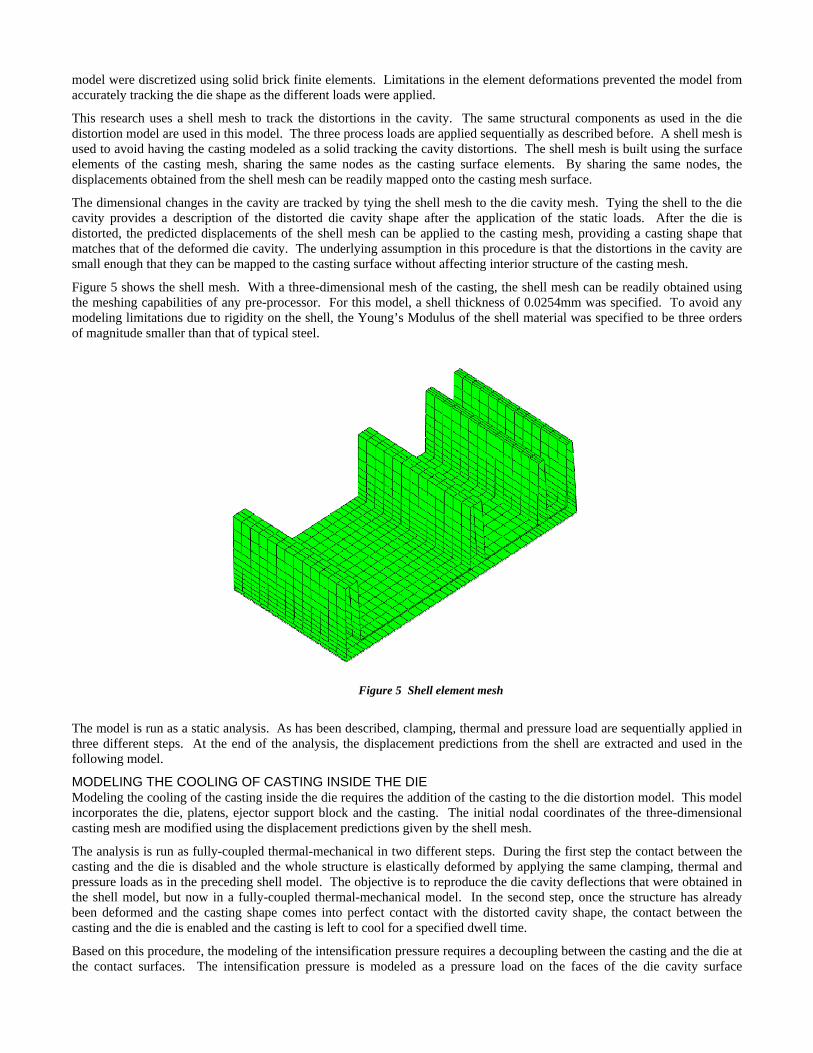
model were discretized using solid brick finite elements. Limitations in the element deformations prevented the model from accurately tracking the die shape as the different loads were applied.
This research uses a shell mesh to track the distortions in the cavity. The same structural components as used in the die distortion model are used in this model. The three process loads are applied sequentially as described before. A shell mesh is used to avoid having the casting modeled as a solid tracking the cavity distortions. The shell mesh is built using the surface elements of the casting mesh, sharing the same nodes as the casting surface elements. By sharing the same nodes, the displacements obtained from the shell mesh can be readily mapped onto the casting mesh surface.
The dimensional changes in the cavity are tracked by tying the shell mesh to the die cavity mesh. Tying the shell to the die cavity provides a description of the distorted die cavity shape after the application of the static loads. After the die is distorted, the predicted displacements of the shell mesh can be applied to the casting mesh, providing a casting shape that matches that of the deformed die cavity. The underlying assumption in this procedure is that the distortions in the cavity are small enough that they can be mapped to the casting surface without affecting interior structure of the casting mesh.
Figure 5 shows the shell mesh. With a three-dimensional mesh of the casting, the shell mesh can be readily obtained using the meshing capabilities of any pre-processor. For this model, a shell thickness of 0.0254mm was specified. To avoid any modeling limitations due to rigidity on the shell, the Young’s Modulus of the shell material was specified to be three orders of magnitude smaller than that of typical steel.
Figure 5 Shell element mesh
The model is run as a static analysis. As has been described, clamping, thermal and pressure load are sequentially applied in three different steps. At the end of the analysis, the displacement predictions from the shell are extracted and used in the following model.
MODELING THE COOLING OF CASTING INSIDE THE DIE Modeling the cooling of the casting inside the die requires the addition of the casting to the die distortion model. This model incorporates the die, platens, ejector support block and the casting. The initial nodal coordinates of the three-dimensional casting mesh are modified using the displacement predictions given by the shell mesh.
The analysis is run as fully-coupled thermal-mechanical in two different steps. During the first step the contact between the casting and the die is disabled and the whole structure is elastically deformed by applying the same clamping, thermal and pressure loads as in the preceding shell model. The objective is to reproduce the die cavity deflections that were obtained in the shell model, but now in a fully-coupled thermal-mechanical model. In the second step, once the structure has already been deformed and the casting shape comes into perfect contact with the distorted cavity shape, the contact between the casting and the die is enabled and the casting is left to cool for a specified dwell time.
Based on this procedure, the modeling of the intensification pressure requires a decoupling between the casting and the die at the contact surfaces. The intensification pressure is modeled as a pressure load on the faces of the die cavity surface
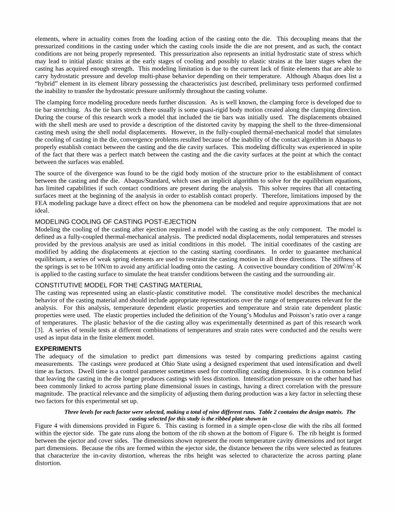
elements, where in actuality comes from the loading action of the casting onto the die. This decoupling means that the pressurized conditions in the casting under which the casting cools inside the die are not present, and as such, the contact conditions are not being properly represented. This pressurization also represents an initial hydrostatic state of stress which may lead to initial plastic strains at the early stages of cooling and possibly to elastic strains at the later stages when the casting has acquired enough strength. This modeling limitation is due to the current lack of finite elements that are able to carry hydrostatic pressure and develop multi-phase behavior depending on their temperature. Although Abaqus does list a “hybrid” element in its element library possessing the characteristics just described, preliminary tests performed confirmed the inability to transfer the hydrostatic pressure uniformly throughout the casting volume.
The clamping force modeling procedure needs further discussion. As is well known, the clamping force is developed due to tie bar stretching. As the tie bars stretch there usually is some quasi-rigid body motion created along the clamping direction. During the course of this research work a model that included the tie bars was initially used. The displacements obtained with the shell mesh are used to provide a description of the distorted cavity by mapping the shell to the three-dimensional casting mesh using the shell nodal displacements. However, in the fully-coupled thermal-mechanical model that simulates the cooling of casting in the die, convergence problems resulted because of the inability of the contact algorithm in Abaqus to properly establish contact between the casting and the die cavity surfaces. This modeling difficulty was experienced in spite of the fact that there was a perfect match between the casting and the die cavity surfaces at the point at which the contact between the surfaces was enabled.
The source of the divergence was found to be the rigid body motion of the structure prior to the establishment of contact between the casting and the die. Abaqus/Standard, which uses an implicit algorithm to solve for the equilibrium equations, has limited capabilities if such contact conditions are present during the analysis. This solver requires that all contacting surfaces meet at the beginning of the analysis in order to establish contact properly. Therefore, limitations imposed by the FEA modeling package have a direct effect on how the phenomena can be modeled and require approximations that are not ideal.
MODELING COOLING OF CASTING POST-EJECTION Modeling the cooling of the casting after ejection required a model with the casting as the only component. The model is defined as a fully-coupled thermal-mechanical analysis. The predicted nodal displacements, nodal temperatures and stresses provided by the previous analysis are used as initial conditions in this model. The initial coordinates of the casting are modified by adding the displacements at ejection to the casting starting coordinates. In order to guarantee mechanical equilibrium, a series of weak spring elements are used to restraint the casting motion in all three directions. The stiffness of the springs is set to be 10N/m to avoid any artificial loading onto the casting. A convective boundary condition of 20W/m2-K is applied to the casting surface to simulate the heat transfer conditions between the casting and the surrounding air.
CONSTITUTIVE MODEL FOR THE CASTING MATERIAL The casting was represented using an elastic-plastic constitutive model. The constitutive model describes the mechanical behavior of the casting material and should include appropriate representations over the range of temperatures relevant for the analysis. For this analysis, temperature dependent elastic properties and temperature and strain rate dependent plastic properties were used. The elastic properties included the definition of the Young’s Modulus and Poisson’s ratio over a range of temperatures. The plastic behavior of the die casting alloy was experimentally determined as part of this research work [3]. A series of tensile tests at different combinations of temperatures and strain rates were conducted and the results were used as input data in the finite element model.
EXPERIMENTS The adequacy of the simulation to predict part dimensions was tested by comparing predictions against casting measurements. The castings were produced at Ohio State using a designed experiment that used intensification and dwell time as factors. Dwell time is a control parameter sometimes used for controlling casting dimensions. It is a common belief that leaving the casting in the die longer produces castings with less distortion. Intensification pressure on the other hand has been commonly linked to across parting plane dimensional issues in castings, having a direct correlation with the pressure magnitude. The practical relevance and the simplicity of adjusting them during production was a key factor in selecting these two factors for this experimental set up.
Three levels for each factor were selected, making a total of nine different runs. Table 2 contains the design matrix. The casting selected for this study is the ribbed plate shown in
Figure 4 with dimensions provided in Figure 6. This casting is formed in a simple open-close die with the ribs all formed within the ejector side. The gate runs along the bottom of the rib shown at the bottom of Figure 6. The rib height is formed between the ejector and cover sides. The dimensions shown represent the room temperature cavity dimensions and not target part dimensions. Because the ribs are formed within the ejector side, the distance between the ribs were selected as features that characterize the in-cavity distortion, whereas the ribs height was selected to characterize the across parting plane distortion.

Table 2 DOE Matrix Run Pressure (bars) Time (s) 1 170 112 170 73 170 94 340 115 680 96 680 77 340 98 340 79 680 11
Figure 6 Casting dimensions in millimeters (2º draft on interior walls formed by the insert and 1º draft on walls formed by the insert
The nominal intensification pressure level of 680 bars represents the upper limit the laboratory machine can provide. The lower pressure level is approximately half machine injection capacity and nearly no intensification pressure.
The runs were randomized and a series of castings were produced using the parameters of run 1 to get the die to a quasi-steady thermal state. Batches of 30 castings were produced for each of the different 9 cases. The last 20 were used for the dimensional analysis to allow the die to reach quasi-steady thermal state after the change in process conditions. Actual cycle times for each casting, shot weights, casting weights and furnace temperature were recorded for each casting.
CASTING MEASUREMENTS A Coordinate Measurement Machine (CMM) was used to measure the dimensions. A fixture based on the 3-2-1 principle was designed and built to secure the castings properly during the measurements. Figure 7shows the six gauging locations on the casting that were contacted by the fixture. The CMM measurements consisted in recording the coordinates of a series of points on the different casting features. Figure 8 shows the selected casting features used to characterize the casting distortion.
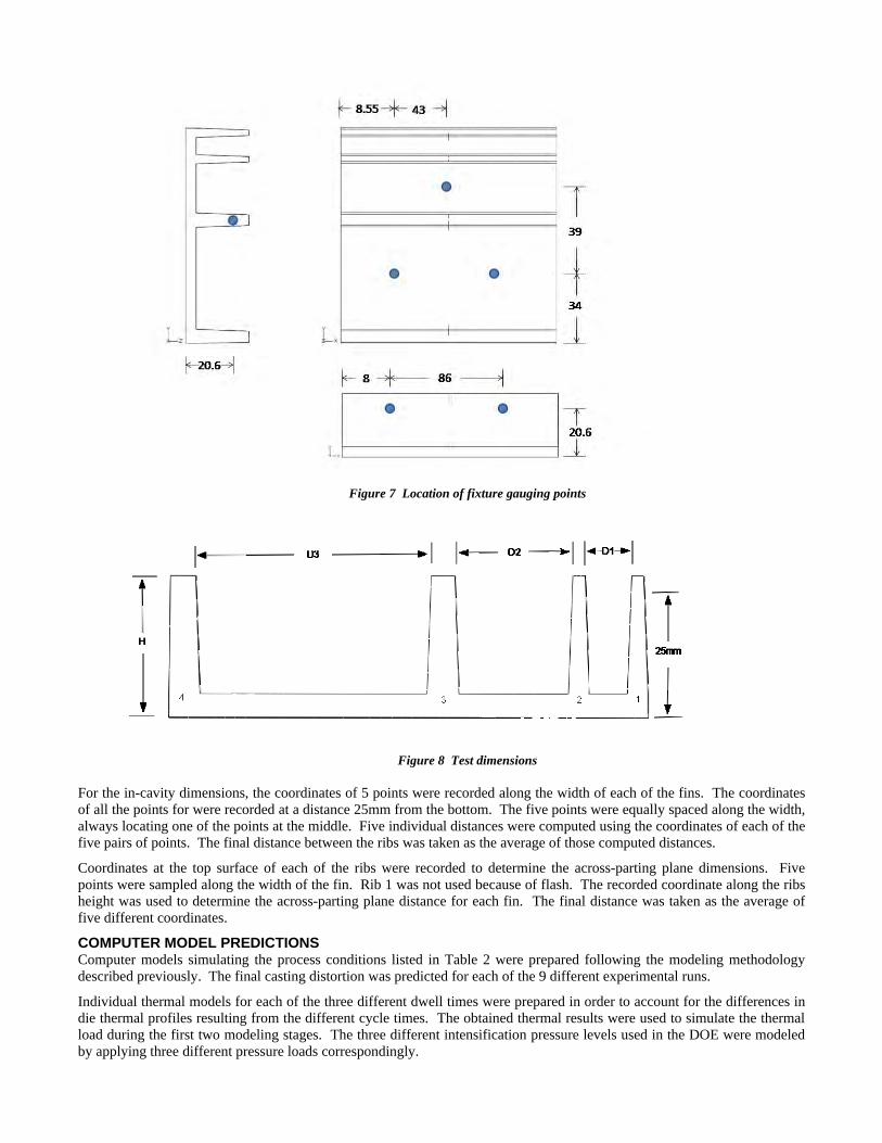
Figure 7 Location of fixture gauging points
Figure 8 Test dimensions For the in-cavity dimensions, the coordinates of 5 points were recorded along the width of each of the fins. The coordinates of all the points for were recorded at a distance 25mm from the bottom. The five points were equally spaced along the width, always locating one of the points at the middle. Five individual distances were computed using the coordinates of each of the five pairs of points. The final distance between the ribs was taken as the average of those computed distances.
Coordinates at the top surface of each of the ribs were recorded to determine the across-parting plane dimensions. Five points were sampled along the width of the fin. Rib 1 was not used because of flash. The recorded coordinate along the ribs height was used to determine the across-parting plane distance for each fin. The final distance was taken as the average of five different coordinates.
COMPUTER MODEL PREDICTIONS Computer models simulating the process conditions listed in Table 2 were prepared following the modeling methodology described previously. The final casting distortion was predicted for each of the 9 different experimental runs.
Individual thermal models for each of the three different dwell times were prepared in order to account for the differences in die thermal profiles resulting from the different cycle times. The obtained thermal results were used to simulate the thermal load during the first two modeling stages. The three different intensification pressure levels used in the DOE were modeled by applying three different pressure loads correspondingly.

The fully-coupled thermal-mechanical models were run to completion using 64-bit Windows-based work stations. The running time for the computer models varied based on the simulated dwell time, taking 15, 19 and 21 days for the 7, 9 and 11 seconds simulated dwell time respectively. The running times were rather long because the maximum step size was controlled not to exceed 0.010 seconds. This restriction in step size was imposed by design in order to avoid numerical errors in the stress field due to large temperature differences within steps.
The distortion predictions were analyzed as if the castings were measured by a CMM in the same manner as the actual castings. A coordinate transformation is required to express the final distorted nodal coordinates of the casting relative to the same coordinate system defined by the fixture used in the experimental measurements. The coordinate system established by the fixture during the measurements was mathematically constructed using the final distorted coordinates of six nodes in the casting located the closest to the gauging points. The procedure followed is essentially that described by Caulk in [17]. Since a symmetric model was used in the simulations only three nodes were sampled along the casting width. The nodes were chosen to be equally spaced as in the CMM measurements with the middle point always located at the symmetry plane. Details of the transformation can be found in [18].
RESULTS Box plots of each dimension determined from the simulation and from the experiment are shown in Figure 9. The data are presented as a percentage of the nominal cavity dimension. Since the comparison is against the die dimension and not the target part dimension, all values are slightly less than 100%.
It is clear from inspection of the box plots that the differences in median are all very small. With the exception of H4 the difference is typically 0.2% to 0.3% which corresponds to 0.002 - 0.003in/in. The difference with H4 is over 1% and is probably due to factors not addressed in the experiment. This difference will be discussed in greater detail later in the paper. The other observation that can be drawn is that the variability in the data is similar for simulation and ecperiment, with the simulation data showing more spread than measurements in several cases.
The measurement data can be analyzed with statistical techniques and an analysis of variance (ANOVA) using a general linear model including pressure, cycle time, furnace temperature, shot weight, and all interactions was performed. A correlation analysis showed that casting weight was correlated with pressure (r = 0.8, p=0) so it was eliminated from the analysis to avoid colinearity problems. Also since cycle time, furnace temperature and shot weight were random factors and not controlled, by chance of the data the cycle time - shot weight interaction could not be estimated.
A summary of the effects and interactions resulting from the ANOVA is provided in Table 3. For purposes of constructing the table, an effect of interaction was classified as significant if p<0.12. The choice of p value is arbitrary. The interaction plots for all
6 measured dimensions are shown in Figure 10 -
Figure 12.
It is not surprising that pressure is significant for all cross parting plane dimensions and for D3, the larger inter rib spacing. Shot weight is also significant for all dimensions due likely to the influence of shot weight on both the thermal load and the distribution of pressure in the cavity. Dwell is significant only for D2 while the dwell*pressure interaction is significant for all but D1.
It is interesting that the only items significant for the D1 (smallest inter rib distance) are shot weight and several interactions with the process nuisance variables. Pressure, Dwell, and Pressure*Dwell, the quantities that the simulation predicts, are not significant suggesting that factors other than those included in the simulation determine this particular dimension.
In summary, generally the measured dimensions are determined by pressure, shot weight, the pressure*dwell interaction, and the pressure*shot weight interaction. Other interactions contribute in specific cases.

Figure 9 Comparison of Measured and Predicted Dimensions
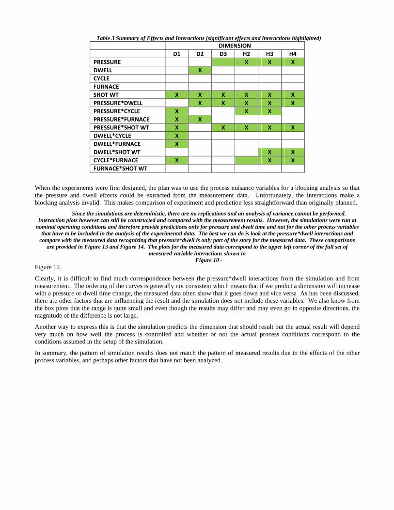
Table 3 Summary of Effects and Interactions (significant effects and interactions highlighted) DIMENSION
D1 D2 D3 H2 H3 H4
PRESSURE X X X
DWELL X
CYCLE
FURNACE
SHOT WT X X X X X X
PRESSURE*DWELL X X X X X
PRESSURE*CYCLE X X X
PRESSURE*FURNACE X X
PRESSURE*SHOT WT X X X X X
DWELL*CYCLE X
DWELL*FURNACE X
DWELL*SHOT WT X X
CYCLE*FURNACE X X X
FURNACE*SHOT WT
When the experiments were first designed, the plan was to use the process nuisance variables for a blocking analysis so that the pressure and dwell effects could be extracted from the measurement data. Unfortunately, the interactions make a blocking analysis invalid. This makes comparison of experiment and prediction less straightforward than originally planned.
Since the simulations are deterministic, there are no replications and an analysis of variance cannot be performed. Interaction plots however can still be constructed and compared with the measurement results. However, the simulations were run at
nominal operating conditions and therefore provide predictions only for pressure and dwell time and not for the other process variables that have to be included in the analysis of the experimental data. The best we can do is look at the pressure*dwell interactions and
compare with the measured data recognizing that pressure*dwell is only part of the story for the measured data. These comparisons are provided in Figure 13 and Figure 14. The plots for the measured data correspond to the upper left corner of the full set of
measured variable interactions shown in Figure 10 -
Figure 12.
Clearly, it is difficult to find much correspondence between the pressure*dwell interactions from the simulation and from measurement. The ordering of the curves is generally not consistent which means that if we predict a dimension will increase with a pressure or dwell time change, the measured data often show that it goes down and vice versa As has been discussed, there are other factors that are influencing the result and the simulation does not include these variables. We also know from the box plots that the range is quite small and even though the results may differ and may even go in opposite directions, the magnitude of the difference is not large.
Another way to express this is that the simulation predicts the dimension that should result but the actual result will depend very much on how well the process is controlled and whether or not the actual process conditions correspond to the conditions assumed in the setup of the simulation.
In summary, the pattern of simulation results does not match the pattern of measured results due to the effects of the other process variables, and perhaps other factors that have not been analyzed.

Figure 10 Interactions for D1 and D2 Measurements
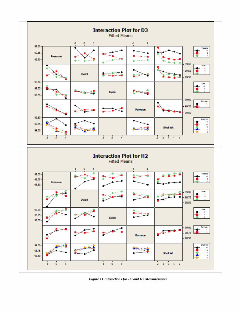
Figure 11 Interactions for D3 and H2 Measurements
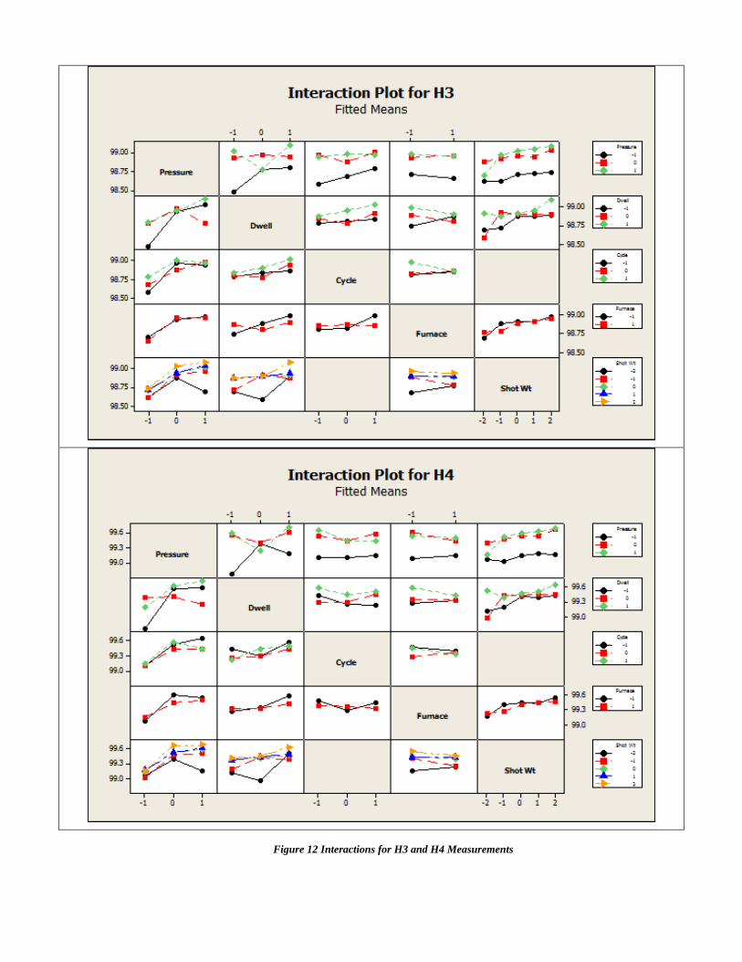
Figure 12 Interactions for H3 and H4 Measurements

Experimental Simulation
Figure 13 Prediction-Measurement Comparisons, D1, D2, D3

Experimental Simulation
Figure 14 Prediction-Measurement Comparisons, H2, H3, H4
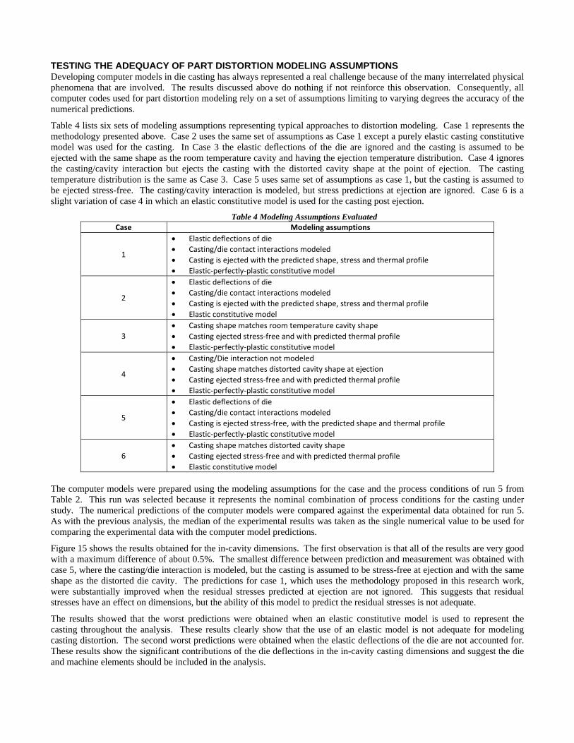
TESTING THE ADEQUACY OF PART DISTORTION MODELING ASSUMPTIONS Developing computer models in die casting has always represented a real challenge because of the many interrelated physical phenomena that are involved. The results discussed above do nothing if not reinforce this observation. Consequently, all computer codes used for part distortion modeling rely on a set of assumptions limiting to varying degrees the accuracy of the numerical predictions.
Table 4 lists six sets of modeling assumptions representing typical approaches to distortion modeling. Case 1 represents the methodology presented above. Case 2 uses the same set of assumptions as Case 1 except a purely elastic casting constitutive model was used for the casting. In Case 3 the elastic deflections of the die are ignored and the casting is assumed to be ejected with the same shape as the room temperature cavity and having the ejection temperature distribution. Case 4 ignores the casting/cavity interaction but ejects the casting with the distorted cavity shape at the point of ejection. The casting temperature distribution is the same as Case 3. Case 5 uses same set of assumptions as case 1, but the casting is assumed to be ejected stress-free. The casting/cavity interaction is modeled, but stress predictions at ejection are ignored. Case 6 is a slight variation of case 4 in which an elastic constitutive model is used for the casting post ejection.
Table 4 Modeling Assumptions Evaluated Case Modeling assumptions
1
Elastic deflections of die
Casting/die contact interactions modeled
Casting is ejected with the predicted shape, stress and thermal profile
Elastic‐perfectly‐plastic constitutive model
2
Elastic deflections of die
Casting/die contact interactions modeled
Casting is ejected with the predicted shape, stress and thermal profile
Elastic constitutive model
3
Casting shape matches room temperature cavity shape
Casting ejected stress‐free and with predicted thermal profile
Elastic‐perfectly‐plastic constitutive model
4
Casting/Die interaction not modeled
Casting shape matches distorted cavity shape at ejection
Casting ejected stress‐free and with predicted thermal profile
Elastic‐perfectly‐plastic constitutive model
5
Elastic deflections of die
Casting/die contact interactions modeled
Casting is ejected stress‐free, with the predicted shape and thermal profile
Elastic‐perfectly‐plastic constitutive model
6 Casting shape matches distorted cavity shape
Casting ejected stress‐free and with predicted thermal profile
Elastic constitutive model
The computer models were prepared using the modeling assumptions for the case and the process conditions of run 5 from Table 2. This run was selected because it represents the nominal combination of process conditions for the casting under study. The numerical predictions of the computer models were compared against the experimental data obtained for run 5. As with the previous analysis, the median of the experimental results was taken as the single numerical value to be used for comparing the experimental data with the computer model predictions.
Figure 15 shows the results obtained for the in-cavity dimensions. The first observation is that all of the results are very good with a maximum difference of about 0.5%. The smallest difference between prediction and measurement was obtained with case 5, where the casting/die interaction is modeled, but the casting is assumed to be stress-free at ejection and with the same shape as the distorted die cavity. The predictions for case 1, which uses the methodology proposed in this research work, were substantially improved when the residual stresses predicted at ejection are not ignored. This suggests that residual stresses have an effect on dimensions, but the ability of this model to predict the residual stresses is not adequate.
The results showed that the worst predictions were obtained when an elastic constitutive model is used to represent the casting throughout the analysis. These results clearly show that the use of an elastic model is not adequate for modeling casting distortion. The second worst predictions were obtained when the elastic deflections of the die are not accounted for. These results show the significant contributions of the die deflections in the in-cavity casting dimensions and suggest the die and machine elements should be included in the analysis.
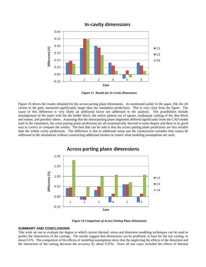
Figure 15 Results for In Cavity Dimensions
Figure 16 shows the results obtained for the across parting plane dimensions. As mentioned earlier in the paper, H4, the rib closest to the gate, measured significantly larger than the simulation predictions. This is very clear from the figure. The cause of this difference is very likely an additional factor not addressed in the analysis. The possibilities include misalignment of the insert with the die holder block, die and/or platens out of square, inadequate cooling of the shot block and runner, and possibly others. Assuming that the insert/parting plane alignment differed significantly from the CAD model used in the simulation, the cross parting plane predictions are all systematically skewed to some degree and there is no good way to correct or compare the results. The best that can be said is that the across parting plane predictions are less reliable than the within cavity predictions. The difference is due to additional setup and die construction variables that cannot be addressed in the simulations without constructing additional meshes no matter what modeling assumptions are used.
Figure 16 Comparison of Across Parting Plane Dimensions SUMMARY AND CONCLUSIONS This work set out to evaluate the degree to which current thermal, stress and distortion modeling techniques can be used to predict the dimensions of die castings. The results suggest that dimensions can be predicted, at least for the test casting, to about 0.5%. The comparison of the effects of modeling assumptions show that the neglecting the effects of die distortion and the interaction of the casting decrease the accuracy by about 0.25%. Since all test cases included the effects of thermal

distortion, these results do not address the relative contribution of temperature and mechanical loads on the predicted dimensions. The results also suggest that an elastic material model is adequate for post ejection cooling, but is not a good assumption for modeling the casting while in the die.
From a practical simulation perspective, modeling of the stress state of the cooling casting while in a die that is dynamically changing shape is a very expensive calculation that, at least with the models used in this research, does not improve the prediction of final casting dimensions. It appears that there are still too many simplifying assumptions to adequately estimate the stresses. Ignoring the in-cavity stresses while tracking cavity distortion is computationally much less expensive and provides as good or better dimensional predictions. This does not address the residual stress issue however.
The use of a shell mesh to capture the distorted cavity shape appears to work, but leaves unaddressed other issues related to modeling the effects of pressure on solidification of the casting and on the casting die interaction during solidification and cooling.
Perhaps the most important insight from the work is the demonstration of the statistical significance of variability in process variables (shot weight, furnace temperature, cycle time particularly shot weight) on dimensions. These variables interact significantly with the controlled process variables. Basically, this means that the use of simulation results to predict the small changes in dimensions on the order of a few thousands of an inch is not dependable unless the process is very well controlled, the die is accurately made, and the setup is very carefully managed. Variability introduced by process and setup factors that are not part of the simulation produce changes in dimensions that are on the same order as the controlled factors. The simulation results may be perfectly accurate, but the results obtained may not correspond to measurements due to variation in other factors. Good process control is essential if simulation is to be a meaningful tool for dimensional control.
ACKNOWLEDGMENTS The authors would like to acknowledge the US Department of Energy ESMART program for its support of this work. They also thank the NADCA computer modeling task group for their valuable suggestions throughout this research.
REFERENCES 1. Karve, A., Dimensional control of die castings, in Industrial Engineering. 1998, The Pennsylvania State University 2. Garza, H.A., of loads in die casting and prediction of die deflections, in Mechanical Engineering. 1996, The Ohio State
University: Columbus, Ohio. 3. Garza-Delgado, A., K. Kabiri-Bamoradian, and R.A. Miller, Gleeble Determination of Elevated-temperature Mechanical
Properties of an Aluminum A380.0 Die Casting Alloy in the As-cast Condition. NADCA Transactions, 2008. 4. Barone, M.R. and D.A. Caulk, Analysis of Thermo-Mechanical Distortion in Die Casting. NADCA Transactions, 1999. 5. Caulk, D.A. and M.R. Barone, dieCAS—Thermal Analysis Software for Die Design: Modeling Approach, NADCA
Transactions, 1993. 6. Sequeira, W.K., Prediction and validation of distortion and residual stresses in an aluminum high pressure diecasting
with considerations to die casting process related variables. NADCA Transactions, 2005. 7. Hedge, K., et al., Analysis of die casting die deflections: part I, modeling and simulation. NADCA Transactions, 1995. 8. Hedge, K., et al., FEM analysis of die casting die deflections: part II, results. NADCA Transactions, 1995. 9. Choudhury, A., Study of the effects of platen size on die deflections. NADCA Transactions, 1997. 10. Miller, R.A., et al., Computer Modeling and Experimental Validation of the Performance of In-board Locks and Proud
Inserts. NADCA Transactions, 1997. 11. Chayapathi, A., V. Kesavan, and R.A. Miller, The Effects of Structural Die and Machine Variables on Die Deflection.
NADCA Transactions, 1999. 12. Ragab, A., K. Kabiri-Bamoradian, and R.A. Miller, Modeling Part Distortion and Residual Stresses in Die Casting
Process. NADCA Transactions, 2001. 13. Ragab, A., K. Kabiri-Bamoradian, and R.A. Miller, Part Distortion and Stress Prediction in Die Casting Process:
Sensitivity Analysis. NADCA Transactions, 2004. 14. Murugesan, K., et al., Effect of Die, Cavity and Toggle Locations on Tie bar Forces, Toggle Forces and Parting Plane
Separation. NADCA Transactions, 2005. 15. Murugesan, K., K. Kabiri-Bamoradian, and R.A. Miller, An experimental verification of the effect of die location on the
tie bar load imbalance. NADCA Transactions, 2007. 16. Osborne, M., J. Brevick, and R.A. Miller, Analysis of Effects of Die Casting Process Control on Casting Dimensional
Variability. NADCA Transactions, 1995. 17. Caulk, D.A., Computer Modeling Keynote. NADCA Transactions, 2007. 18. Garza-Delgado, A., A study of casting distorion and residual stresses in die casting, in Industrial and Systems
Engineering. 2007, Ohio State University: Columbus, Ohio.

Appendix D: Determination of Elevated Temperature Mechanical
Properties of an Aluminum A380.0 Die Casting Alloy in As‐Cast
Condition
This paper is subject to revision. Statements and opinions advanced in this paper or during presentation are the author’s and are his/her responsibility, not the Association’s. The paper has been edited by NADCA for uniform styling and format. For permission to publish this paper in full or in part, contact NADCA, 241 Holbrook, Wheeling, Illinois, 60090, and the author.
Determination of Elevated-Temperature Mechanical Properties of an Aluminum A380.0 Die Casting Alloy in the As-Cast Condition
Abelardo Garza-Delgado, Khalil Kabiri-Bamoradian, R. Allen Miller
The Ohio State University
ABSTRACT Computer model predictions of casting distortion and residual stresses using finite element analyses have become a valuable tool over the past years. The obtained predictions have provided useful insights into the effects of process parameters on casting final distortion as well as on tooling performance. The predictions can be a valuable piece of information as well when trying to size die cavities to produce castings with the correct dimensions and within the tolerances. However, the adequacy of the computer model predictions is strictly related to the material properties used to represent the different mechanical components comprising the model. Currently, the mechanical properties of casting materials from the solidus to room temperature are a lacking piece of information needed to refine the deformation and residual stress predictions given by the computer models. Furthermore, accurate representation of the casting material temperature and strain-rate dependency, especially at high temperatures, represents also a much needed piece of information in the material’s property definition. This paper presents the results a series of elevated-temperature tensile tests done to determine the temperature and strain rate-dependent mechanical properties for the die casting aluminum alloy A380.0. The tests were carried out using a Gleeble 1500 thermo-mechanical simulator available at The Ohio State University. The selected specimens for the tests were used in the as-cast conditions. The tensile tests were conducted at different combinations of temperatures and constant strain rates characteristic of the solidification conditions commonly found in die castings. The obtained results confirmed the typical plastic behavior of casting aluminum alloys at elevated temperatures. It was observed that perfect plasticity was obtained for temperatures higher than 250 ºC. The strain-rate dependency became more evident at temperatures higher than 150 ºC. INTRODUCTION Computer modeling in the die casting industry has become a popular tool among successful die casters. Die casters have benefited from the model predictions by looking at fill patterns, evolution of temperature profiles in casting and tooling, distortion of machine components and tooling, etc., all available at the analyst’s computer desk. The development of these computer models has been tightly related to the increase in the complexity of the mathematical models used to describe the involved physical phenomena and to the developments in computer hardware required to solve such complex systems of equations. These developments have allowed computer models to provide better representations of the analyzed systems and to give more accurate and reliable predictions. However, in spite of the great improvements in the mathematical models and computer hardware, the accuracy of the computer model predictions has been limited due to the lack of material properties used to represent the behavior of the different components in the model. This is particularly true in the case of part distortion analyses, which rely on accurate constitutive models to represent the casting material behavior. These analyses are aimed at predicting the mechanical and thermal response of the casting during solidification, and require accurate physical, thermal and mechanical properties for the casting alloy throughout the whole solidification and cooling range. On the one hand the physical and thermal properties for most die casting alloys are available in the literature and their magnitudes can be readily found. Currently, computer codes have been developed that can compute these properties using thermodynamical principles as presented by Saunders et al [1], Miettinen [2] and Miettinen et al [3]. These codes have been readily incorporated in casting CAE packages such as ProCAST [4]. On the other hand however, the mechanical properties and their dependency on temperature and material characteristics such as strain rate are a lacking piece of information for die casting alloys. The required material properties comprise what is called the casting constitutive model in the finite element models and are used for computing the stresses based on the developed elastic, inelastic and thermal strains. Thus, in order to

improve the accuracy of the stress predictions in casting distortion analyses, the mechanical properties of the die casting alloys must be determined. The aim of this research article is to present the results of an experimental project done to determine the elevated-temperature mechanical properties of the aluminum die casting alloy A380.0. The main contribution of the results presented here consists of a series of stress vs. strain curves at different temperatures and strain rates that can be used with die casting distortion computer models. The article is structured as follows. First, a review of the literature concerning casting alloys material properties is presented. A detailed description of the methodology used to carry out the tensile tests is presented next. The next section describes the results of the mechanical tests. Lastly, the final section is devoted to the discussion and conclusions of this project. LITERATURE REVIEW DIE CASTING ALLOYS The microstructures and mechanical properties of a wide range of die casting alloys were determined in an experimental project carried out at Worcester’s Polytechnic Institute [5]. The aim of the project was to provide die casting designers with material data for product design purposes. Tensile and fatigue test specimen were produced following ASTM standards. The tensile tests were conducted at 25 ºC, 100 ºC and 200 ºC with a test velocity of 0.05in/min. The specimen were heated using a heating chamber attached to the testing machine and the axial strain was determined by a extensometer placed in contact with the specimen. The results of this comprehensive project were reported as a series of stress vs. strain curved at the three temperature conditions for the wide range of die casting alloys. These data primarily address the properties of the casting material under operating conditions. The creep behavior of three aluminum die casting alloys was determined by Jaglinski et al [6]. The selected aluminum alloys were B-390 (Al-17%Si-4%Cu-0.5%Mg), eutectic Al-Si alloy (Al-13%Si-3%Cu-0.2%Mg) and Al-17%Si-0.2%Cu-0.5%Mg alloy. The objective of the study was to provide product designers with creep material data for engine design, as many of these components work under high temperatures and creep and relaxation might be observed during engine operation. As-cast tensile test specimens were used to perform the creep tests. The specimen were heated at 220 ºC, 260 ºC and 280 ºC. Constant creep load uniaxial tests were done using a dead weight lever frame, where strain was measured using axial extensometers securely attached to the specimen’s gage section. The results were presented as a series of strain vs. time curves for the selected alloys at the different temperature conditions. ALUMINUM CASTING ALLOYS Singer et al [7] conducted an experimental work to determine the mechanical properties of a variety of hypoeutectic Al-Si alloys below and in the solidus temperature. The purpose of the study was to provide experimental data that would assist in explaining the phenomenon of hot-shortness. A total of ten different alloys were tested, including super-purity aluminum. The specimen were heated using a resistance tube furnace that slid on the testing apparatus, providing uniform heating throughout the specimen’s length. The experimental results showed that the tensile strength of the tested Al-Si alloys decreases gradually as the temperature increases above 400 ºC, reaching finite magnitudes at the solidus temperature. The mechanical behavior of various Al-Cu alloys at solidifying and just-solidified temperature conditions was determined by Wisniewski et al [8]. The goal of the study was to develop an adequate fracture criterion to predict hot tearing for Al-Cu solidifying alloys. The percentage Cu content was varied from 2.5 to 7.5%. Rectangular bars 13x51mm were tested at strain rates that ranged from 1x10⁻⁵ to 1x10⁻¹ s-1. The specimen were mounted onto a fixture in an Instron machine. The tests were carried at constant extension rates. The obtained results show that, at all strain rates, the maximum stress decreased as the Cu content was increased. The mechanical behavior of an Al-4.5%Cu-Mg-Ti alloy in the mushy zone was determined in an experimental study conducted by Vicente-Hernandez et al [9]. The main objective was to determine an adequate testing procedure to determine the visco-plastic mechanical behavior of aluminum alloys in the mushy zone in order to provide solidification computer models with reliable material data for gap formation predictions. The developed test consisted in the pushing of a needle at a constant rate into a solidifying ingot. The cooling conditions in the mold were controlled carefully to obtain vertical isotherms. The described test provided records of applied force versus needle displacement at different temperatures. The experimental data was fitted to the Norton-Hoff power law model. The results showed a remarkable match between the measured displacements and the displacements predicted by the simulation. DIRECT CHILL CASTING ALLOYS Van Haaften et al [10] conducted an experimental study to determine the mechanical properties of AA1050, 113104 and AA5182 DC aluminum casting alloys. The objective was to obtain a Power law model using the experimental data that can be used in computer models to predict thermal stresses and deformation in DC ingots. A series of tensile tests at different

temperatures and strain rates were performed using a Gleeble 1500 and a Gleeble 3500. Non-cylindrical specimen 10mm in diameter and 95mm long, with a reduced 8mm diameter at the center were used for the testing. The obtained data was fitted to the extended Ludwik power law and to the Garofalo’s hyperbolic-sine models. The flow stress at steady-state creep conditions for AA3103 aluminum alloy was determined by Farup et al [11]. The goal of the experimental study was to obtain the parameters of the Garofalo’s model for use in DC thermal-mechanical finite element models. Non-cylindrical specimens being 10mm in diameter, 90mm long and a reduced 8mm diameter at the specimen’s center were used. The obtained results were successfully used to determine the parameters of the Garofalo’s equation. The mechanical properties under compression, tension and cyclical compression for AA582 Direct Casting aluminum alloy were determined by Alhassan-Abu et al [12]. The objective was to determine the parameters of the Garofalo’s equation for use in computer modeling of thermal-mechanical stress in Direct Casting ingots. The tests were carried out using a Gleeble 1500 machine. The results obtained were used to determine the parameter of the Garofalo’s hyperbolic-sine model. METHODOLOGY This section describes the procedure followed to determine the elevated temperature mechanical properties for the die casting alloy A380.0. A detailed description of all the steps taken to carry out this experimental project is provided. Issues such as machine and specimen selection, the selected design of experiments matrix, production and preparation of specimens and testing methodology are presented in the following paragraphs. MACHINE AND SPECIMEN SELECTION Based on the approaches and results reported in the literature review, the Gleeble machine was selected to perform the high temperature tensile tests. As reported in the cited articles, the Gleeble thermo-mechanical simulator is a reliable piece of equipment that can readily perform tensile tests at the required temperatures and strain rates. The reliability of the control system in controlling temperature, jaw velocity and loading force made the Gleeble 1500 an excellent choice for the project. The Gleeble system is a high-strain-rate, high temperature testing machine where a solid specimen is held horizontally by water cooled grips, through which electric current is introduced to resistance heat the test specimen [13]. Fig. 1 shows the schematic of a typical Gleeble test. Specimen temperature is monitored by a thermocouple that is spot welded to the specimen’s surface. The temperature of the specimen is controlled by a function generator using the readings provided by the thermocouple. The direct-resistance heating system of the Gleeble machine can heat specimen at rates of up to 10,000 ºC/s. Due to this capability, this machine can perform hot tensile tests several times faster than conventional methods. Radial strain measurements are readily done by attaching a dilatometer that monitors the reduction in area as the specimen is being tensioned.
Fig. 1 Schematics of a typical Gleeble test [10]
The specimen design is shown in Fig. 2. The selected shape corresponds to the suggested design for conducting fatigue tests for die casting alloys and was chosen based on the shapes described in the articles cited in the literature review section. The common denominator in those designs was the use of a cylindrical specimen with a reduced diameter at the center. The reduction in area at the center was done in order to guarantee that the maximum strained region is at the specimen’s center. Additionally, as reported by Walsh et al [14], quadratic temperature profiles are typical of a Gleeble test, where the maximum temperature is located at the specimen’s center and the water cooled grips define the lowest temperature points. Thus, the quadratic temperature profile together with the reduction in area guarantees that the region of failure is located at the specimen’s center, eliminating the need for a gage length.

Fig. 2 Schematic of the selected specimen
The radial strains were determined by the reduction in area readings provided by a dilatometer attached at the specimen’s center as shown in Fig 1. The radial strains were computed by using the following expression
oradial D
Dln2
Eq. 1
where D is the current diameter
oD is the starting diameter
The radial strains were then converted to axial strains by using the following expression
radial
allongitudin
Eq. 2
where is the Poisson’s ratio The true stresses were readily computed by dividing the applied force by the reduced cross-sectional area as shown in the following expression
A
F
Eq. 3
The describe procedure relied in two main assumptions. One is the assumption of a homogeneous temperature distribution throughout the specimen’s length. The other assumption is a homogenous cross-sectional shape. Both assumptions generate non-uniform flow stresses along the specimen’s length, leading to inaccuracies in the computed stresses and strain rates. This was recognized by Farup et al [15] where the effects of those in-homogeneities were investigated. An axis-symmetric model representing the specimen in their tests was modeled in Abaqus. The obtained visco-plastic properties from the experiments were assigned to the material. Three conditions were studied: one representing the same temperature and shape in-homogeneities as in the experiments, another one assuming a non-cylindrical specimen but with a uniform longitudinal temperature profile and the last one assuming a cylindrical specimen but with the parabolic temperature profile characteristic of their tests. The obtained results showed that the variation in the visco-plastic strain rate along the radius varies as much as 12.5%, with a maximum at the center. It was recognized that the major source of variation was the parabolic temperature

profile, contributing more than the non-cylindrical shape to the observed radial differences. It can therefore be expected that the obtained strain-rates in the experiments carry an error of at least 12.5% due to the above mentioned in-homogeneities. SELECTION OF TESTING CONDITIONS A design of experiments was proposed where the specimen temperature and strain rate were the main design variables. The selected temperatures ranged from 25 ºC to 500 ºC, having a total of ten levels. The strain rates were determined by analyzing the cooling conditions at different regions on a typical die casting using the following expression
dt
dT
dt
d
Eq. 4
where is the coefficient of thermal expansion Cooling rates from a computational thermal analysis of different regions of a solidifying casting were extracted and Eq. 1 was used to calculate the strain rates. The obtained results produced strain rates that ranged from 1x10⁻⁶ to 1x10⁻² s-1. Given the results obtained, five different levels for the strain rate were selected. Because of the different levels obtained for the two design variables, a Hexagonal design was selected [16]. Table 1shows the design matrix. In order to have statistical significance on the results, it was decided to conduct 5 replications for each of the 20 cases, making a total of 100 tests.
Run Temperature (ºC) Strain rate (s-1) 1 500 3.16E-04
2 486 2.26E-03 3 444 1.28E-02 4 381 4.62E-02 5 304 9.16E-02 6 221 9.16E-02 7 144 4.63E-02 8 81 1.28E-02 9 39 2.27E-03
10 25 3.17E-04 11 25 3.17E-04 12 39 4.42E-05 13 81 7.83E-06 14 144 2.16E-06 15 221 1.09E-06 16 304 1.09E-06 17 381 2.16E-06 18 444 7.80E-06 19 486 4.40E-05 20 263 3.16E-04
Table 1. Experimental array for tensile tests SPECIMEN PRODUCTION AND PREPARATION The specimen were produced using an existing insert available at The Ohio State University. The insert design allowed the production of two specimen per shot. The production was carried out continuously during one shift at Empire Die Casting Co., Inc. located in Macedonia, Ohio. A total of 800 specimen were die cast with an average cycle time of 40s and a shot weight of 0.5kg. The information regarding alloy chemistry is shown in Table 2.
Si Fe Cu Mn Mg Cr Zn Ni Ti Pb Sn V Al 8.92 0.801 3.28 0.17 0.0386 0.097 1.72 0.0643 0.0361 0.0341 0.0156 0.00477 84.82
Table 2. Aluminum alloy chemical composition

After production, the specimen were trimmed. Runners, biscuit and any excessive flash were manually removed. The runner and biscuit were removed using a rubber hammer, while the flash was removed using a vertical band saw. Radiographs were taken on all specimen to guarantee that only the best would be tested. The specimen were X-rayed. The radiographs showed that the majority of the specimens had shrinkage porosity at the grip ends, while very little porosity was detected at the reduced cross-sectional area. Out of the 800 specimen produced 370 were selected for testing. The selected specimen were machine-threaded using a threading die. The specific thread used was ½-20. The finer pitch was selected to maximize the number of threads engaged during testing to avoid stripping the threads. The machine-threading was also done to guarantee proper alignment between the axes produced by the threads on both grip ends. After threading the specimen were polished. Polishing was done using a rotating brush, with the main intention of removing residual flash at the parting plane. A smooth surface finish was obtained after polishing was completed. TESTING PROCEDURES As can be seen in Table 1, the 20 cases required different combinations of temperatures and strain rates. Two different approaches, namely constant jaw velocity and constant force, were developed based on the way the required strain rates were achieved and were used to perform the tests. A description of the procedures is provided in the following paragraphs. The strain rate is a mechanical material behavior characteristic that provides a measure of the rate of strengthening or softening of the material under a given set of loading conditions. This rate of strengthening or softening may or may not be constant depending on the way the material responds as the plastic deformation is taking place. Constant strain rates at temperatures below creeping are usually achieved by loading the material under a constant rate of displacement and can be estimated by using the following expression
l
v
dt
d
Eq. 5
where v is the jaw velocity
l is the deformed length Because most aluminum alloys start creeping at temperatures around 300 ºC, all the test cases at temperatures below 300 ºC were conducted under constant jaw velocities. As can be seen from Eq. 5 the magnitude of the strain rate is proportional to the magnitude of the jaw velocity. A series of room temperature tests were performed to determine the correlation between the jaw velocity and the obtained radial strain rate measured at the specimen’s center. The jaw velocity was varied progressively by orders of magnitude and the strain was measured by a dilatometer and recorded by the Gleeble’s data acquisition system. With the time history of the recorded strain, the strain rates were computed numerically. Fig. 3 shows the strain-time and strain rate-time plots for a case where the jaw velocity was 0.001mm/s. The top figure shows that the radial strain came to be in the order of 1x10⁻³ mm/mm, while the strain rate was about 1x10⁻⁶ s-1. The fact that the strain rate is 3 orders of magnitude smaller can be explained by the order of magnitude of the time scale, which is about 1x10³ s. The strain rate results were plotted in a histogram and the results are shown in Fig. 4. The histogram clearly depicts that the radial strain rates at the specimen’s center were all in the order of 1x10⁻⁶ s-1.
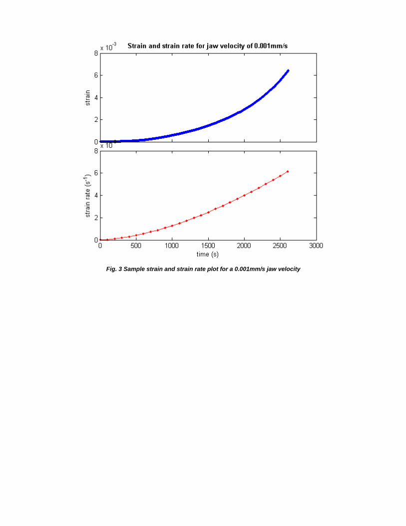
Fig. 3 Sample strain and strain rate plot for a 0.001mm/s jaw velocity

Fig. 4 Sample histogram of strain rate distribution for a 0.001mm/s jaw velocity
As can be noticed from the results shown, there exists a clear correlation between the jaw velocity and the achieved radial strain rates. In order to get a more comprehensive correlation plot, a series of tests with various jaw velocities were done and the results were processed as described before. From the log-log scatter plot shown in Fig. 5, a linear correlation between the jaw velocity and the achieved radial strain rate can be observed. Although the correlation plot shown in Fig. 5 was generated using the results of room temperature tests, this correlation was found to be valid and vary only slightly for temperatures up to 260 ºC. Therefore, the obtained plot was used as a basis to carry out all the test cases where the specimen’s temperature was under 300 ºC.
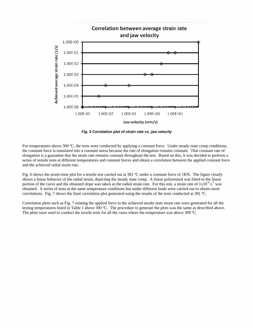
Fig. 5 Correlation plot of strain rate vs. jaw velocity
For temperatures above 300 ºC, the tests were conducted by applying a constant force. Under steady state creep conditions, the constant force is translated into a constant stress because the rate of elongation remains constant. That constant rate of elongation is a guarantee that the strain rate remains constant throughout the test. Based on this, it was decided to perform a series of tensile tests at different temperatures and constant forces and obtain a correlation between the applied constant force and the achieved radial strain rate. Fig. 6 shows the strain-time plot for a tensile test carried out at 381 ºC under a constant force of 1KN. The figure clearly shows a linear behavior of the radial strain, depicting the steady state creep. A linear polynomial was fitted to the linear portion of the curve and the obtained slope was taken as the radial strain rate. For this test, a strain rate of 1x10⁻⁶ s-1 was obtained. A series of tests at the same temperature conditions but under different loads were carried out to obtain more correlations. Fig. 7 shows the final correlation plot generated using the results of the tests conducted at 381 ºC. Correlation plots such as Fig. 7 relating the applied force to the achieved steady state strain rate were generated for all the testing temperatures listed in Table 1 above 300 ºC. The procedure to generate the plots was the same as described above. The plots were used to conduct the tensile tests for all the cases where the temperature was above 300 ºC.

Fig. 6 Sample strain vs. time curve for a 1.0KN force at 381 ˚C
Fig. 7 Correlation plot of strain rate vs. force at 381 ˚C
RESULTS The tensile tests were carried out using the correlation plots shown in previous section as reference. Before any test was conducted, all one hundred test case numbers were randomized to minimize the effect of the many sources of error. The selection of the specimen for each test was done randomly as well to minimize the effect of the specimen production process on the results. Care was exercised to choose specimen from the whole batch. The tests were conducted over a one month period, five months after the specimen were produced. The five-month period was considered long enough to minimize the effects of any aging taking place in the metal. In the meantime before the bars were tested, the specimen were stored at room temperature under controlled conditions.

After each test was conducted, the raw data from the Gleeble data acquisition system was numerically filtered using a running average technique. Each of the curves shown in Fig. 8 to Fig. 10 represents the numerical average of the five replications performed at each of the twenty different testing conditions listed in Table 1. The average was numerically computed strain-wise. The curves have been grouped in three figures to facilitate visualization due to the wide range of stress and strain scales among the many curves. Fig. 8 shows the curves representing the results for temperatures between 25 ºC and 144 ºC. Fig. 9 shows the curves representing the results for temperatures between 221 ºC and 381 ºC. Lastly, Fig. 10 shows the curves representing the results for temperatures between 444 ºC and 500 ºC. As can be seen from Fig. 8, the strain rate effects do not play a significant role for temperatures below 100 C. The strain rate effects start to be seen at 144 C, where the material experiences a decrease in the flow stress and the rate of strain hardening. The elongation magnitudes can be seen to vary quite substantially and might be attributed to the different levels of porosity content and distribution among the specimen. As shown in Fig. 9, perfect plasticity was obtained for strain rates about 1x10⁻⁶ s-1 at temperatures above 220 C. Above this temperature magnitude, the strain rate has a marked effect on the yield stress, where the smallest strain rates result in smaller yield stresses. The curves in this figure also show the significant impact temperature has on the yield and flow stresses. The curves show that the total elongation of the bars was largely dependent on the temperature magnitude. Fig. 10 shows the material response at the three highest temperature levels tested. As in the previous cases, the strain rate effects have a significant impact on the magnitude of the flow stress. From the curves it can be seen that the flow stress at 444 ºC and 1x10⁻⁶ s-1 is smaller in magnitude to any of the two curves at 486 ºC. These results seem to suggest that even one order of magnitude difference in strain rate can produce a higher yield stress even for a 40 ºC temperature difference.
Fig. 8 Stress vs. strain curves at 25 ˚C, 39 ˚C, 81 ˚C and 144 ˚C
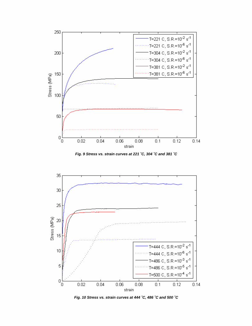
Fig. 9 Stress vs. strain curves at 221 ˚C, 304 ˚C and 381 ˚C
Fig. 10 Stress vs. strain curves at 444 ˚C, 486 ˚C and 500 ˚C

CONCLUSIONS Material properties are one of the most important pieces of information when building a finite element model. The constitutive equations that relate stress to strain are a function of the material constitutive model used. If the constitutive model used does not represent adequately the response of the analyzed part, the stress and force predictions will be highly questionable. The lack of mechanical properties at temperatures relevant for solidification analysis was the motivation to carry out a project to determine the constitutive model for the die casting alloy A380.0. Test bars were die cast and specimens were qualitatively selected based radiography results. A series of stress-strain curves at different combinations of temperature and strain rate were obtained. The tests were carried out using displacement and force control modes in a Gleeble thermo-mechanical simulator. The displacement control mode was used for temperatures below creep (about 300 ºC), whereas the force control model was used for temperature above creep. Calibration curves for both modes of control were developed to conduct the tests. The results obtained showed the large dependency of the flow stress on both, temperature and strain rate. Temperature and strain rate effects on flow stress showed a more marked effect at temperatures greater than 150 ºC. Perfect plasticity was obtained at temperatures about 220 ºC. The obtained trends suggested that strain rate has a greater impact on flow stress at temperatures above 300 ºC. Its effects were even more notorious at the highest temperatures tested, where an order of magnitude increase in strain rate can result in a higher flow stress even when the temperature is 40 ºC smaller. As far as elongation is concerned, a greater scatter was observed at the lowest temperatures tested. The elongation was seen to be largely a function of the temperature, where greater magnitudes were obtained the higher the temperature. The scatter of the elongation results was smaller at the highest temperatures tested. ACKNOWLEDGMENTS We would like to thank Rick Tomazin formerly of DCD for the help provided in modifying the tooling used in this project. We are grateful to Mark Kubicki from Empire Die Casting for all the help provided in developing the cycle time parameters needed and for the production of the test bars. We would like to thank the Materials Science and Engineering Department at The Ohio State University for allowing us to use the Gleeble 1500 for conducting the tests. The successful completion of this project was largely a function of their help and we would like to express our gratitude. This research was funded in part by the US Department of Energy ESMART program, award number DE-FC36-04GO14230. This support is much appreciated. REFERENCES
1. Saunders, N. L.-P. (2003). Modelling of the thermophysical and physical properties relevant to solidification. Modeling of Casting, Welding and Advanced Solidification Processes X (pp. 669-676). The Minerals, Metals & Materials Society.
2. Miettinen, J. (1997). Calculation of solidification-related thermophysical properties for steels. Metallurgical and
Materials Transactions B , 28B, 281-297.
3. Miettinen, J. L. (1994). Calculation of thermophysical properties of carbon and low alloyed steels for modeling of solidification processes. Metallurgical and Materials Transactions B , 25B, 909-916.
4. ProCAST.
5. Makhlouf, M. A. (2000). Microstructures and properties of aluminum die casting alloys. North American Die
Casting Association.
6. Jaglinski, T. L. (2004). Creep behavior of Al-Si die cast alloys. Journal of Engineering Materials and Technology , 126, 378-383.
7. Singer, R. C. (1946). Properties of the aluminum-silicon alloys at the temperatures in the region of the solidus.
Journal of Institute of Metals , 33-54.
8. Wisniewski, P. B. (1991). Tensile behavior of solidifying aluminum alloys. Modeling of Casting, Welding and Advanced Solidification Processes V (pp. 259-264). The Minerals, Metals & Materials Society.

9. Vicente-Hernandez, P. D. (1995). Mushy state behavior: rheological characterization and influence on air gap formation. Iron and Steel Institute of Japan International , 35 (6), 805-812.
10. Van Haaften, W. M. (2002). Constitutive behavior of as-cast AA1050, AA3104 and AA5182. Metallurgical and
Materials Transactions A , 33A, 1971-1980.
11. Farup, I. D. (2000). Gleeble machine determination of creep law parameters for thermally induced deformations in aluminum DC casting. Journal of Thermal Stresses , 47-58.
12. Alhassan-Abu, A. W. (2003). Determination of constitutive behavior of as cast AA5182 for deformations that occur
during direct chill casting using the Gleeble 1500 machine. Materials Science and Technology , 19, 55-61.
13. Tensile Testing (Second ed.). (2004). American Society for Metals.
14. Walsh, D. C. (1986). Temperature measurements in resistance-heated specimens: longitudinal gradients. Welding Journal , 65, 184-192.
15. Farup, I. D. (1998). Inhomogeneities in the stress and strain rate fields during Gleeble testing. First ESAFORM
Conference on Material Forming. Sophia Antipolis, France.
16. Myers, R. M. (1995). Response Surface Methodology. John Wiley & Sons.

Appendix E: Die and Die Casting Machine Computer Simulations:
Modeling, Meshing, Boundary Conditions, and Analysis Procedures

DieandDieCastingMachineComputerSimulations:Modeling,Meshing,BoundaryConditions,and
AnalysisProcedures
Khalil Kabiri-Bamoradian
Center for Die Casting
The Ohio State University
July-2010

i
Contents0. Introduction .................................................................................................................... 1
1. Modeling ........................................................................................................................ 4
1.1 Solid Modeling Procedures .................................................................................... 5 1.2 Modeling Simplifications....................................................................................... 6 1.3 Modeling Contacts ................................................................................................. 6 1.4 Solid Modeling of Components ............................................................................. 7 1.4.1 Analysis Units ................................................................................................... 7
1.4.2 Naming Components ........................................................................................ 8
1.4.3 Constructing Die Casting Models ..................................................................... 8
2. Meshing........................................................................................................................ 37
2.1 Element Types ..................................................................................................... 40 2.2 Meshing of Components ...................................................................................... 41 2.2.1 Inserts .............................................................................................................. 41
2.2.2 Dies ................................................................................................................. 46
2.2.3 Casting Part ..................................................................................................... 48
2.2.4 Platens ............................................................................................................. 49
2.2.5 Tie Bars ........................................................................................................... 50
2.2.6 Toggle Mechanism.......................................................................................... 54
2.2.7 Support Blocks, Back Plates and Pillars ......................................................... 57
2.2.8 Die Casting Machine Base .............................................................................. 58
2.2.9 Die Slides ........................................................................................................ 61
2.2.10 Other Un-common Components of Machine or Dies ................................... 62
2.2.11 Tie Bars Nuts ................................................................................................ 62
2.2.12 Bolt Joints Between Components ................................................................. 63
3. Boundary Conditions and Material Properties ............................................................. 65
3.1 Mechanical Loads ................................................................................................ 65 3.2 Components Constraints ...................................................................................... 66 3.2.1 Tie Bar Constraints ......................................................................................... 66
3.2.2 Ejector and Rear Platens Constraints .............................................................. 67
3.2.3 Cover Paten Constraints .................................................................................. 67
3.2.4 Toggle Mechanism Using Springs .................................................................. 68
3.2.5 Spring Forces on the Die Slides ...................................................................... 69
3.2.6 Casting Part and Dies/Inserts Part Cavity Intensification Pressure ................ 69
3.3 Temperature Calculations .................................................................................... 71 3.3.1 Casting Part, Dies and Inserts Part Cavity Heat transfer Coefficients ............ 71
ii
3.3.2 Outside Dies Heat Transfer Coefficients ........................................................ 71
3.3.3 Contact Heat Transfer Coefficients ................................................................. 73
3.3.4 Heat Removal During Spraying ...................................................................... 73
3.3.5 Heat Transfer from Dies and Insets ................................................................ 76
3.4 Contact Surfaces .................................................................................................. 77 3.4.1 Contact Element Set Definition ....................................................................... 78
3.5 Mechanical and Thermal Properties of Materials ................................................ 80 3.5.1 Defining Thermal Properties ........................................................................... 82
3.5.2 Defining Mechanical Properties .................................................................... 84
3.6 Conversion Table ................................................................................................. 85 4.0 Analyses ..................................................................................................................... 86
4.1 Magmasoft ........................................................................................................... 88 4.1.1 Magmasoft Pre-processor ............................................................................... 89
4.1.2 Magmasoft Mesh Generation .......................................................................... 91
4.1.3 Magmasoft Simulation Run ............................................................................ 91
4.2 Thermal Analysis ................................................................................................. 93 4.2.1 Abaqus Thermal Simulation ........................................................................... 94
4.2.2 Inputs Commands for Thermal Simulation..................................................... 95
4.3 Mechanical Analysis ............................................................................................ 98 4.3.1 Input Commands for Mechanical Analysis ................................................... 100
4.4 Abaqus Run Commands .................................................................................... 103 5. Post-Processing .......................................................................................................... 104
5.1 Magmasoft Post-Processor................................................................................. 105 5.2 Abaqus Post –Processor ..................................................................................... 105 5.2.1 Mesh and Boundary Conditions Display ...................................................... 106
5.2.2 Background Color ......................................................................................... 107
5.2.3 Viewing ......................................................................................................... 108
5.2.4 Deform and Un-deform Shapes of Components ........................................... 108
5.2.5 Contour Plots ................................................................................................ 110
5.2.6 Parting Plane Separation ............................................................................... 113
6. Acknowledgements .................................................................................................... 116
7. References .................................................................................................................. 118
1
0. Introduction The die casting process is a net shape or near net-shape manufacturing process. The liquid
metal is injected into the part cavity inside the inserts/dies under high pressure. The liquid
metal solidifies inside the die then it is ejected as a net shape or near finished part. The inserts
and dies play two rolls in this process, 1) they are the mold for the part, 2) they extract heat
from the liquid metal allowing it to solidify and form the part, and therefore they are cooling
media for the casting part too.
For die casting to be economically competitive and produce large quantities of parts with
reasonable cost, the cycle time has to be short and the scarps has to be keep to a small percent
of total manufactured parts and also after works should be minimal on the parts. The cycle
time consists of following operation;
1) Closing of the dies,
2) Clamping of the dies (application of clamp force),
3) Injecting the molten metal under high pressure,
4) Dwelling or solidification under intensification pressure,
5) Opening of the dies and then rejecting the casting part,
6) Spraying the cavity, dies and inserts with the lubricant, coolant and/or air,
7) Dies stay open and are exposed to air.
Each of these operations will take some seconds or its fractions to be completed; a cycle time
is the addition of times for all of these seven operations. The shortest times are the application
of clamp force and the molten metal injection.. The largest times are spent at the dwell time,
which is the time for part to solidify by removing heat, or at sparing time and subsequent
cooling, which is to cool the dies and inserts. If dwell time can made shorter, as long this
dwell time can produce a satisfactory part, will result in shorter spraying time; and therefore
total cycle will be shorter. The above cycle is repeated to produce as many casting parts as
intended.
The die casting simulation effectively will model the physics involved at each cycle in order

2
to predict the dies, casting part and machine deflections, distortion and stresses. The
simulation model will include the geometry of: casting part, inserts, dies, slides, support/back
plates, pillar supports, platens, tie bars, toggle mechanism, machine base and other
components deemed necessary for structural integrity of the die casting process.
The adjacent components are attached together by bolted joints or welded joints. They come
into contact with each other on the opposing surfaces. The contact surfaces affect both the
load path and heat transfer from one component(s) to the neighboring component(s). The
contacts between two adjacent parts are simulated using contact surfaces. The contacting
surfaces are closed or are in touch with each other when there is a compressive force between
them. These surfaces cannot penetrate into each other. The contacting surfaces open when
there are tension force between them.
At the start of casting or at the first shot to produce the first part, the dies/inserts and die
machine components are at room temperature. In some cases the dies and inserts are heated
using heating lines or external heaters to bring up the dies/inserts temperature near operating
condition. After the first cycle the dies/inserts and other components temperature will start to
rise. It will take a large number of cycles, possibly more than 100 cycles, for the dies/inserts
temperatures to reach to a quasi-steady state temperature, depending on the size of the casting
part, dies and cooling methods.
The change in temperature of dies/inserts can results in non-uniform deformation of
dies/inserts which can affect load pass, and therefore the tie bar forces and parting plane
separation pattern. The temperature changes due to heat removal will results in thermal
forces/loads on the dies/inserts and exert a thermal load on the dies, inserts and machine. This
thermal load is in addition to the mechanical loads, static forces, i.e. clamping and
intensification loads, which is present during each cycle. The mechanical loads are almost
constant during each cycle, but thermal load will change from cycle to cycle until the machine
reaches to the quasi steady state operation condition.
During the injection of molten metal there are dynamic forces, these forces are the spikes of

3
intensification forces due to acceleration and deceleration of the plunger motion. These
dynamic loads will be in addition to the static loads experienced by the dies/inserts and
machine during the clamping and intensification. Dynamics loads can change from cycle to
cycle too.
As can be seen there are there set of loads which is present at each cycle of the die casting
process:
1) Dynamic forces,
2) Static forces,
3) Thermal forces.
At the Center for Die casting at Ohio State University for predicting the deflections and
stresses of the dies and machine assembly, parting plane separations of the dies and inserts,
and tie bar forces, we consider only the static and thermal loads in majority of our
simulations. A first approximation of dynamics loads can be performed by using equivalent
static loads, this means that we can multiply the intensification force by a factor, this factor
can change from 1.5 to 2.5, depending on the machine size and plunger size and motion. In
this way we will have an approximate estimate of what these dynamics forces will do on the
dies/insets separation.
At the Center for Die Casting we have developed special procedure that can be sued to predict
and estimate casting part deformation and stresses
The material properties of the dies, inserts, support blocks, support pillars and machine
components are almost constant and independent of temperature, or they have a weak
temperature dependency in the range of the operating temperature of the dies/inserts and other
attached components, this assumption will simplify the analysis. But the material properties of
casting part form molten to room temperature are strongly dependent on the temperature
which should be included in the analysis.

4
Two types of analysis can be used to simulate the die casting processes, coupled thermo-
mechanical analysis and de-coupled thermo mechanical analysis.
In a decoupled analysis, we can first perform a time transient thermal analysis of the casting
part, dies/insets and other attached components to dies to simulate as many cycles as needed.
The results from this thermal analysis simulation will be the predicted temperature for the
dies/inserts and other components which is included in the thermal model. The next step is to
perform a static analysis, with the given clamp force and intensification pressure plus the
temperature results from the thermal analysis, for the selected cycles. The selected cycles, in
our group, usually are:
A) Cycle 1, which simulates the cold dies/inserts,
B) Cycle 30, which simulates the semi hot dies/inserts,
C) Cycle 100, which simulates the quasi-steady state, or hot dies/inserts
Performing the thermal and static analysis sequentially is called un-coupled thermo-
mechanical analysis. When the mechanical and thermal properties are
temperature dependent, or when the casting part deformation will affect the heat transfer
coefficient and vice–versa or when we are interested in casting parts’ deformation and casting
part stresses and residual stresses coupled thermo-mechanical analysis in essential. This type
of analysis is much more complex and the run times are much longer than un-coupled thermo-
mechanical simulations.
1. Modeling
Modeling and analysis of the die casting processes for an de-coupled thermo-mechanical
analysis involve three major operations:
1) Constructing the solid model of the dies, inserts, tie bars, platens, toggle mechanism,
supports block / back plates, pillar support , machine base and other components as needed.
5
2) Generating mesh from the solid models for heat transfer analysis, i.e. using Abaqus [1], this
model includes at least casting part, dies and inserts and other components if needed.
3) Generating mesh model for static analysis with the given mechanical and thermal loads to
predict displacements and stresses of each component in the assembly model. This model will
include inserts, dies, supports blocks/ back plates, pillar support and die machine components,
which is consists of toggle mechanism, platens, tie bars, guiding pines and machine base and
other machine components that will affect the loading path due to clamp loads.
If solidification analyses are intended STL files of casting part, dies and inserts and other
components are used as input files for solidification simulation using Magmasoft [2] or
Procast [3].
1.1SolidModelingProcedures
A preprocessor is used to generate solid models, Ideas [3] is generally used at the Center for
Die Casting to make the solid models. Abaqus can be also used to generate solid models. The
customers usually provide us with the solid models of components; these models are usually
generated using different solid modelers. The most frequently used CAD or preprocessor
software are Pro/E (4) , Ideas / NX ( Unigraphics) (5) , Catia (6), Autocad (7), Anysys (8),
and Hyperworks (9) , Patran (10), and the solvers are Abaqus, Ansys, and Marc (11)
The solid models that provided by the customers, in general, have more details than needed
for die casting simulations. The first task of the analyst is to simplify the CAD solid models
without compromising the integrity of the structure. These operations usually mean that the
analyst will reconstruct components solid models. In some cases only the two dimensional
drawing will be provided by the customers, in these cases the analyst will construct the solid
models using these two dimensional drawings.
6
1.2ModelingSimplifications
The solid model simplification can include but is not limited to the following rules:
A) The small fillets, and radii can be easily ignored.
B) Cooling/heating line can be modeled as circular sections or they can be modeled as
rectangular duct with equivalent areas. The path of cooling lines can be represented by
segments of the straight lines.
C) Bolt joints can be represented by tied contact or explicitly modeled as bolt joints with pre-
loads.
D) If two components are attached together with many bolts or with weld joints, the two
structures can be modeled as one solid piece.
E) Straight or curved lines and surfaces can be used to represent small details of the parts
geometries
E) The grooves in the platens can be ignored or if needed the thickness of the platen can be
modified to have equivalent stiffness.
If the die casting assembly is symmetric, the symmetry should be utilized. This will
reduce the number of nodes and elements by half. In this case if necessary more details of the
components can be included in the model.
1.3ModelingContacts
In generating the solid model the analyst should provide provision for the contacting surfaces
between/among the components for both thermal and mechanical contacts. The important
contact surfaces will include, but is not limited to the following:
For mechanical load analysis:
a) Contact between the faces of the dies and inserts,
b) Contact between the inserts and dies,
c) Contacts between the faces of the dies (shoe face),
d) Contacts between the ejector die and support block/back plate,

7
e) Contact between the support block/back plate and ejector platen,
f) Contact between the cover die and cover platen,
g) Contact between the slides and inserts and/or dies,
h) Contact between the tie bars and the platens,
i) Contact between the ejector and rear platens the railing of the machine base,
j) Contact between the machine base and ejector and rear platen.
The combined shoe face and inserts face contacting surfaces will make up the parting plane
surface of the dies.
For thermal load analysis
a) Contact between the face of the inserts,
b) Contacts between the inserts and dies,
c) Contacts between the face of the dies.
1.4SolidModelingofComponents
The solid model of each component can be generated one part a time, these components then
can be assembled together to include all the components necessary for a particular analysis.
The following sections describe the steps that may be considered for this purpose
1.4.1AnalysisUnits
In general the standard length unit for CAD models is mm (millimeter). The models can be
generated in this unit but when exported it can be converted to other units. At Center for Die
Casting standard SI units of MKS (meter, kilogram, second) are used for most of the
simulations. In some cases where dimensions of part geometry are small and using meter
length scale can cause numerical problems, the millimeter can be used for the length scale. If
the length unit is in mm, care should be taken to define all other thermal, mechanical and
physical properties in consistent units.
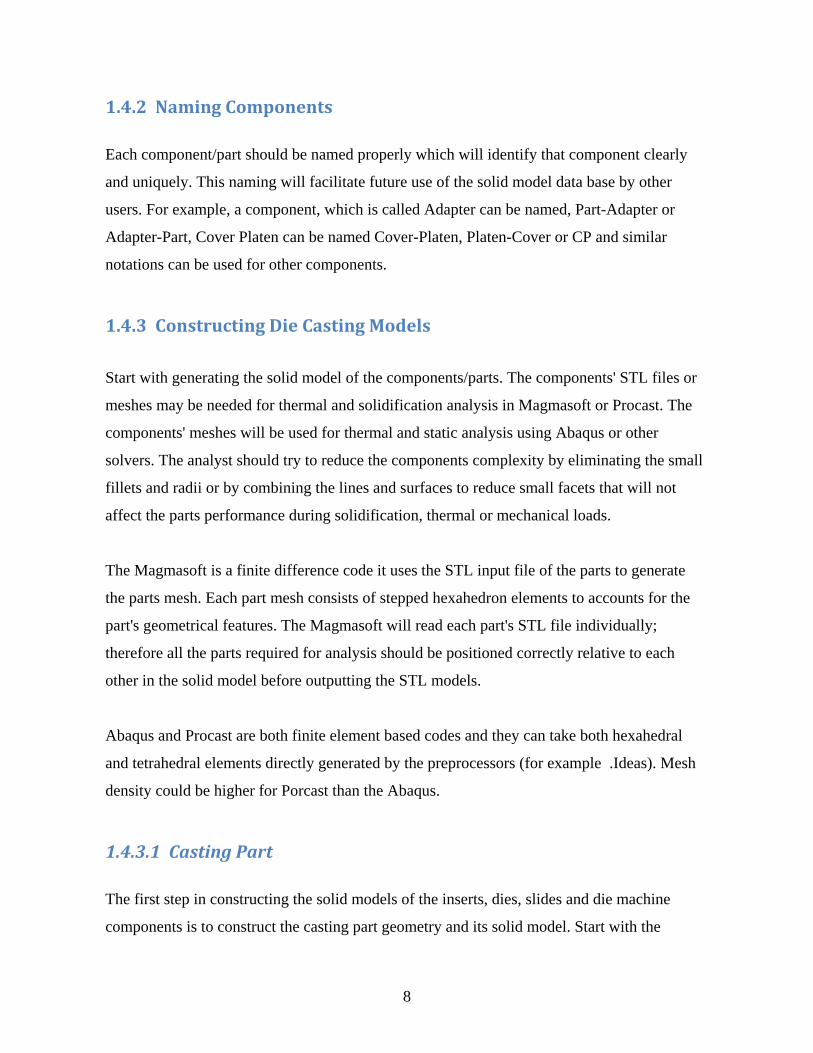
8
1.4.2NamingComponents
Each component/part should be named properly which will identify that component clearly
and uniquely. This naming will facilitate future use of the solid model data base by other
users. For example, a component, which is called Adapter can be named, Part-Adapter or
Adapter-Part, Cover Platen can be named Cover-Platen, Platen-Cover or CP and similar
notations can be used for other components.
1.4.3ConstructingDieCastingModels
Start with generating the solid model of the components/parts. The components' STL files or
meshes may be needed for thermal and solidification analysis in Magmasoft or Procast. The
components' meshes will be used for thermal and static analysis using Abaqus or other
solvers. The analyst should try to reduce the components complexity by eliminating the small
fillets and radii or by combining the lines and surfaces to reduce small facets that will not
affect the parts performance during solidification, thermal or mechanical loads.
The Magmasoft is a finite difference code it uses the STL input file of the parts to generate
the parts mesh. Each part mesh consists of stepped hexahedron elements to accounts for the
part's geometrical features. The Magmasoft will read each part's STL file individually;
therefore all the parts required for analysis should be positioned correctly relative to each
other in the solid model before outputting the STL models.
Abaqus and Procast are both finite element based codes and they can take both hexahedral
and tetrahedral elements directly generated by the preprocessors (for example .Ideas). Mesh
density could be higher for Porcast than the Abaqus.
1.4.3.1CastingPart
The first step in constructing the solid models of the inserts, dies, slides and die machine
components is to construct the casting part geometry and its solid model. Start with the

9
desired working plane (sketch plane). It has been adopted, at the Center for Die Casting, that
the tie bar axis to be in the Z direction, therefore the platens will be located in X-Y plane. The
vertical direction will be Y axis and lateral direction will be X direction. The casting part solid
model is necessary for the construction of the inserts. The solid model of the casting part
could be subtracted from the inserts geometry to create the part cavity in the inserts. Figure
1.1 shows the solid model of an experimental casting part used at the Center. This
Experimental casting part has been used extensively by our research groups both in computer
simulations models and physical experiments. The physical experiments were done in our
facilities at the center. The purposes of experiments are to compare and validate our results
from the computer simulation and actual experiments.
Figure 1.1: Solid model of an experimental part

10
1.4.3.2Inserts
The next step is to construct the inserts. In a solid model maker, for example Ideas, the
working plane (sketch plane) should be selected as one of the planes of the casting part. This
will ensure that when all solid models of parts are made and they are meshed together, they
will be in the same coordinate system for analyses. Some solid model makers use the
technique of joining and partitioning the solid models to created the shape of solid models
.The joining and partitioning solid models have its drawbacks, it is not precise and some times
can create thin volumes, these thin volumes usually can not be meshed or if they are meshed it
will result in degenerated or bad elements, therefore the joining and partitioning should be
avoided.
The overall inserts shapes are square or rectangular blocks that the casting part geometry is
subtracted from them to create the part cavity. The first step is usually to construct the cover
and ejector insert solid models and then remove the casting part from them.
The inserts usually have cooling and/or heating lines. The cooling and heating lines should be
included in the inserts solid models. These lines are circular pipes, but in the simulation they
can be modeled as circular or rectangular pipes. The rectangular pipe shapes will make the
solid model construction easier in this case the area of the rectangular is equal to the area of
the circular pipe. The disadvantage of making pipes rectangular is that if we are interested in
inserts stresses the rectangular pipes will cause higher stress concentration at the cores of the
pipes. In general it is safer to model them as the same shape of the heating or cooling lines.
The addition of the cooling or heating lines will increase the complexity of the solid models
and in essence will increase number of elements in the inserts. The cooling and or heating
lines are essential in removing heat from the insert and cooling them, therefore they should be
a part of the meshed model for thermal analysis. When each volumes or portions of inserts
have been constructed, the solid models should be tested to verify that the constructed solid
model could be meshed with acceptable element quality for particular analyses. This practice
should be followed when solid models for any component are made. The element generation
(meshing) will be described in Chapter 2.
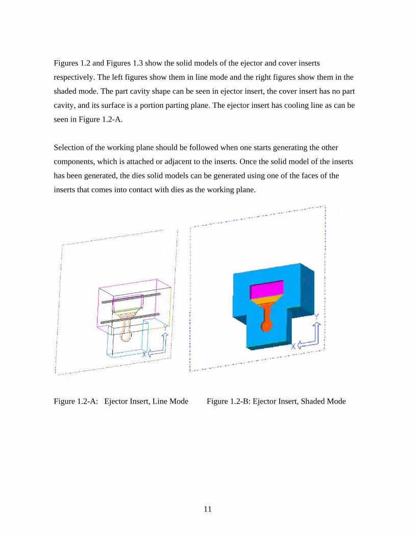
11
Figures 1.2 and Figures 1.3 show the solid models of the ejector and cover inserts
respectively. The left figures show them in line mode and the right figures show them in the
shaded mode. The part cavity shape can be seen in ejector insert, the cover insert has no part
cavity, and its surface is a portion parting plane. The ejector insert has cooling line as can be
seen in Figure 1.2-A.
Selection of the working plane should be followed when one starts generating the other
components, which is attached or adjacent to the inserts. Once the solid model of the inserts
has been generated, the dies solid models can be generated using one of the faces of the
inserts that comes into contact with dies as the working plane.
Figure 1.2-A: Ejector Insert, Line Mode Figure 1.2-B: Ejector Insert, Shaded Mode

12
Figure 1.3-A: Cover Insert, Line Mode Figure 1.3-B: Cover Insert, Shaded Mode
1.4.3.3DiesandPositioning/GuidingPins
In generating the dies models a working plane (sketch plane) should be selected on the
corresponding insert's solid model to construct the dies solid models. For example, starting
with the ejector die, first construct the ejector die, which, in general, at the start will look like
a rectangular or square box, then remove the ejector insert solid model from the ejector die
solid model. Figures 1.4 shows the solid model of the ejector dies, in the line mode and
shaded mode.
The same steps should be followed for the cover die using the cover inserts. The cover
geometry includes the runners that should be included in the cover die model. Figures 1.5
show the cover die and insert models, no runners and biscuits are shown in these figures.
Similar to inserts, the dies also have the cooling and/or heating lines; these lines should be
modeled in a similar way to the cooling and/or heating lines of the inserts. Figures 1.6 show
the cooling lines in the ejector die.

13
Figure 1.4-A: Ejector Die, Line Mode Figure 1.4-B: Ejector Die, Solid Mode
Figure 1.5-A: Ejector Die, Line Mode Figure 1.5-B: Ejector Die, Shaded Mode
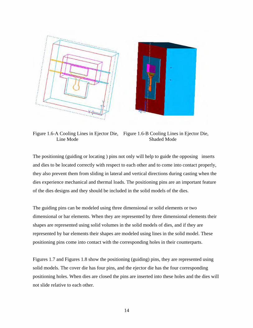
14
Figure 1.6-A Cooling Lines in Ejector Die, Figure 1.6-B Cooling Lines in Ejector Die, Line Mode Shaded Mode The positioning (guiding or locating ) pins not only will help to guide the opposing inserts
and dies to be located correctly with respect to each other and to come into contact properly,
they also prevent them from sliding in lateral and vertical directions during casting when the
dies experience mechanical and thermal loads. The positioning pins are an important feature
of the dies designs and they should be included in the solid models of the dies.
The guiding pins can be modeled using three dimensional or solid elements or two
dimensional or bar elements. When they are represented by three dimensional elements their
shapes are represented using solid volumes in the solid models of dies, and if they are
represented by bar elements their shapes are modeled using lines in the solid model. These
positioning pins come into contact with the corresponding holes in their counterparts.
Figures 1.7 and Figures 1.8 show the positioning (guiding) pins, they are represented using
solid models. The cover die has four pins, and the ejector die has the four corresponding
positioning holes. When dies are closed the pins are inserted into these holes and the dies will
not slide relative to each other.
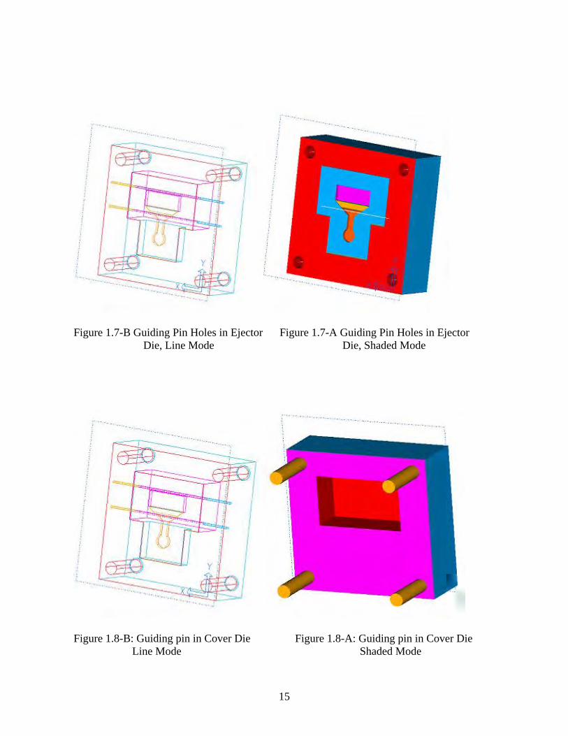
15
Figure 1.7-B Guiding Pin Holes in Ejector Figure 1.7-A Guiding Pin Holes in Ejector Die, Line Mode Die, Shaded Mode
Figure 1.8-B: Guiding pin in Cover Die Figure 1.8-A: Guiding pin in Cover Die Line Mode Shaded Mode

16
In solid model representation of the guiding pins, and pin holes, they will be modeled as a part
of the cover die or ejector die solid model, this depends on the die design and where the pins
are located on the cover or ejector die. Usually the guiding pins are press fitted onto the cover
die and they slide into the ejector die holes. For this reason the pins can be modeled as a part
of the cover die as one piece together (see Figure 1.6 and 1.7).
The interaction of the pins with the holes on the ejector die can be represented by contacting
surfaces. The contacting surfaces modeling will be described in Chapter 3. Modeling the pins,
as a solid model, will expedite the modeling and contact definitions.
To model the locating pins using bar elements will follow procedures that will be explained
for the tie bars using bar elements.
1.4.3.4SlidesDies are called an open-closed dies when there are no slides; Open-closed dies are consists of
inserts and dies only. The dies in Figures 1.4 through 1.8 are open-closed dies. If there are
slides the similar steps, as described for the building inserts and dies should be followed to
construct the solid models of the slides. The slides will be built by selecting a working plane
(sketch plane) on the side of the inserts that comes into contact with the slides. Then the
analyst can start constructing the slides geometry and its solid models. When constructing the
dies solid models with slides, both the inserts and slide solid models should be removed from
the dies solid models. The same procedure can be used to construct the solid models of the
other slides if necessary.
1.4.3.5SupportsBlock,BackPlates,andSupportPillars
The supports blocks, back plates, and support pillars are attached to the ejector die; these
components connect the ejector die to the ejector platen. The clamp forces path goes through
17
these components, and these components will give additional structural support to ejector die
by providing larger contact area between the ejector die and ejector platen, which will results
in less deflection of the ejector platen and reduce parting plane separation. A realistic solid
model representation of these components should be included in the total assembly of dies
and machine. Simplification can be made to the geometry as long as the load path and contact
areas remain almost the same. For example, the support block, pillars and back plate are
usually bolted to the ejector die or to each other; these parts can be modeled as one solid
model attached to the ejector die.
The next step is to construct the support block, back plates, and support pillars solid models.
Since the support block / back plate/ pillars come into contact with the ejector die, a working
plane (sketch plane) should be selected on the ejector die. After the selection of working plane
the construction of the supports/ back plates / support pillars geometry and solid models can
begun.
Figures 1.9 show the support block of ejector die, in this design there are no support pillars or
back plate. The shapes of the support block / back plate /support pillars patterns varies
depending on the die machine and die designs, some have pillars and some have railings on
the sides. In large dies they have many pillars to support the back of the dies / inserts. In some
die designs the supports pillars can be found on both the ejector side and cover side and in
some designs they use back plate as an additional support for ejector die and some designs do
not have this feature. If back plate bolted in many locations and it behaves as one piece with
the ejector die the ejector die and support plate ca be modeled as monolithic or one piece
component.

18
Figure 1.9-A: Ejector Die and Support Figure 1.9-B: Ejector Die and Support Block
Line Mode Block, Shaded Mode
1.4.3.6Platens
Most of the die casting machines have three platens, cover platen, ejector platen, and rear
platens, there are two platen machines that they have only cover and ejector platens. In this
manual we describe three machine platens in details and the same can be followed for two
platen machines.
In general the platens shapes are rectangular blocks, from which four cylinders with the size
of the tie bars are removed. The platen also have groove and cut to mount the dies. If there
are other features, which influence the structural integrity and the response of the ejector
platen; those should also be included in the solid model. The cover, ejector platens shapes and
their thickness’ can differ from each other.
The ejector platen comes in contact with the support bock / back plates, therefore a working
plane (sketch plane) should be selected on the support block/ back plate solid models to begin
the construction of the ejector platen geometry and its solid models.
19
The ejector platens have mounts to be attached to the toggle mechanism. The toggle
mechanism applies the predefined clamp load on the machine. This clamp forces can be
applied on the ejector platen as boundary conditions or through toggle mechanism solid model
based through special loading sequences. The clamp forces can be represented as a
distributed load on the applied pad location or load can be applied through toggle mechanism
which will be represented by solid or bar elements. Applying the clamp load though the solid
or bar elements are the standard modeling approach at Center for Die Casting. The ejector
platen is free to slide on the tie bars, the interaction between the tie bars and ejector platen
should be modeled using contact surfaces. Also the bottom surface of ejector platen slides on
a railing of the machine base. The ejector platen can move up but it cannot move down, this
motion will be modeled using contact surface definitions.
The cover platen comes into contact with the cover die; therefore a working plane (sketch
plane) should be selected on the cover die solid models to start constructing the cover platen
geometry and its solid model. The cover platen is also looks like a rectangular box, from
which four cylinders with the size of the tie bars are removed. The cover platen also has the
hole or slot for the shot sleeves and has special geometry around and near shot hole, and the
geometry around this hole sometimes should be considered in the solid model to include any
structural contribution from its geometry (cover platens are thinner around the sot sleeve
holes). The cover platen is attached to the machine base by bolts or welded to it, therefore
cover platen is not free to mode side ways and upward.
Figures 1.10 show the cover platen (in orange) and ejector platen (in purple), along with the
cover and ejector die and the support block.
The tie bars are fastened to the cover platen through nuts in a die machine. The tie bar
connection to the cover platen can be achieved in two ways:
a) If the tie bars modeled as solid model then it will be meshed using three dimensional or
solid elements. The tie bar end nodes and the cover platen nodes on the perimeter of the holes
should have common nodes or they should be tied together. To represent the nut stiffness, a

20
plate or solid model of the nut can be constructed. If the nuts are represented by plate
elements the nuts and the end face of the tie bars should have common nodes or tied together.
If the nuts are modeled using solid elements the inner nodes of the nuts and outer nodes of the
extended tie bars should have common nodes or tied together.
b) If two dimensional or bar element is used to represent tie bars, then plate elements can be
used to represent the nuts. Each nut should have a center node where the tie bar will attach to
it. The nuts will have common nodes with the nodes on the perimeter of the tie bar holes on
the cover platen. In addition radial or spoke shaped bar elements should attach the center node
of the nuts to the edge nodes of the nuts. The nut models will have common nodes with the
cover platen or nodes are tied to the platen. The thickness of the nut models and their material
property will be the same as the nut thickness and nut material properties of machine tie bars.
The connection steps will be explained in tie bar section
Figure 1.10-A: Cover and Ejector Platens Figure 1.10-B: Cover and Ejector Platens and Dies, Line Mode and Dies, Shaded Mode .
21
The rear platen model is also looks like a rectangular or square block from which four
cylinders with the same diameter of the tie bars has been removed. The tie bars are attached at
one end to the cover platen and the other end of the tie bars are connected the rear platen. The
same models as described for the cover platens can be used to connect tie bars to rear platen.
The toggle mechanism applies clamp load from one side on the ejector platen and on the other
side on the rear platen, provision should be taken similar to ejector platen for toggle
mechanism.
1.4.3.7TieBars
Tie bars can be modeled using solid models or lines. The solid model representations will be
meshed with the three dimensional elements and the line representations will be meshed using
two dimensional or bar elements.
1.4.3.7.1TieBarsasSolidModels
In this case, the tie bars will be constructed as cylindrical objects and they will be meshed
using three dimensional elements, tetrahedron or hexahedron elements. Provisions should be
taken for the areas of the tie bars where they come into contact with the platens. It is a good
modeling practice to divide the full length of tie bar to at least into six sections. It is preferable
that these sections are made longer than the platens thicknesses. Descriptions of these sections
will start from the rear platen toward the cover platen:
First section; if rear platen model is included in the solid models then this section comes into
contact with the tie bar holes in the rear platen. If no rear platen is included in the assembly,
then all end nodes are fixed in all directions. The length of this section will be at least equal to
the thicknesses of tie bar holes in the rear platen.
Second section is the part between rear and ejector platens. The length of this section will be
equal to the length between the rear platen and ejector platen.
Third section is the portion of tie bar that comes into contact with the tie bar holes in ejector
platen. The length of this portion will be at least equal to the length of tie bar holes in the
ejector platen.

22
Fourth and fifth section will represent the area between the ejector and cover platens. The
section between the ejector and cover platen are sectioned into two solid models at Center for
die Casting. The portioning plane is at the location of parting plane dies, the faces at this
location are tie together. The forces of these nodes at this portioning plane are one of the
outputs of analyses and each tie bar force is calculated from appropriate output node set.
Sixth section is the area of the tie bars that come into contact with the cover platen. The length
of this section will be equal at least to the length of tie bars holes in cover plate. The total
length of the tie bar is the summation of these six part parts. If the nut models are to be
included, both at cover and rear platens, then seventh and eighth sections are also needed to
represent these portions of the bars where they come into contact with the nuts.
The sections of the tie bars that are coming into contact with the platens will be modeled
using contact surfaces. In some case to simplify the models; for example for the cover platen
area and rear platen areas, these contacts can be reprinted by tying the surfaces together or
using tied nodes, but it is not recommended. The nuts models can be modeled as described in
the platen section. If the nuts are modeled as solids then seventh and eighth sections of the tie
bars are attached to the nuts and they will have common nodes or tied nodes. Figures 1.11
show the solid models of tie bars and the nuts, in this model the nuts have been molded as
circular doughnut shape objects.

23
Figure 1.11-B: Tie Bars as Solid Model Figure 1.11-A: Tie Bars as Solid Model Line Mode Shaded Mode
1.4.3.7.2TieBarasLineModels
The line representation of tie bars will be meshed using bar elements, in this form the tie bar
will be partitioned into at least six sections. These section will the same as the sections
described for the solid models.
The contact representation of the bar elements with the platens can be modeled using the
following approach:
Making points or nodes or mesh the surface of the tie bar holes in the platen and the tie bars
using at least four or five segments. Construct. radial lines, between the points (nodes) on the
tie bars and the points (nodes) on the surface of the tie bar holes in the platen, by attaching
one point (node) on the tie bar to all the radial points (nodes) on the inside surface of the tie
bar holes in the platen. The shape of these radial lines will look like spoke wheels and their
length is equal to the radius of the tie bars. When these lines are meshed they have nodes at
both ends of the bar. But the ends nodes they will be have common nodes with the tie bars
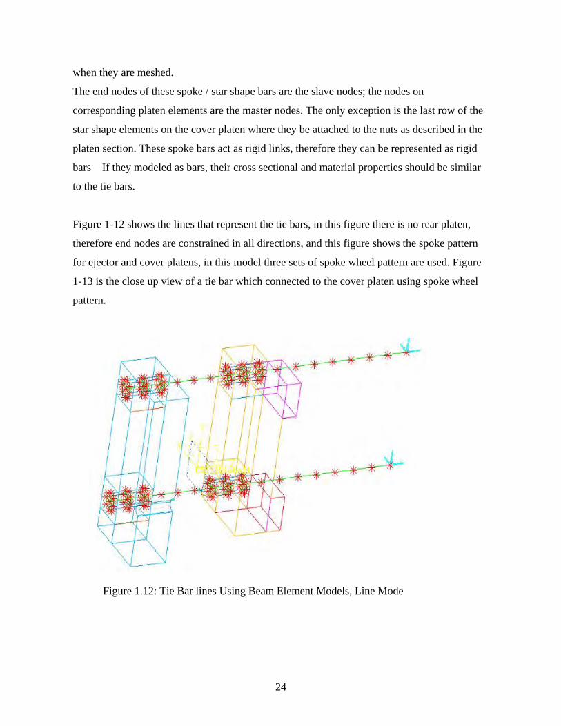
24
when they are meshed.
The end nodes of these spoke / star shape bars are the slave nodes; the nodes on
corresponding platen elements are the master nodes. The only exception is the last row of the
star shape elements on the cover platen where they be attached to the nuts as described in the
platen section. These spoke bars act as rigid links, therefore they can be represented as rigid
bars If they modeled as bars, their cross sectional and material properties should be similar
to the tie bars.
Figure 1-12 shows the lines that represent the tie bars, in this figure there is no rear platen,
therefore end nodes are constrained in all directions, and this figure shows the spoke pattern
for ejector and cover platens, in this model three sets of spoke wheel pattern are used. Figure
1-13 is the close up view of a tie bar which connected to the cover platen using spoke wheel
pattern.
Figure 1.12: Tie Bar lines Using Beam Element Models, Line Mode

25
Figure 1.13: Close up View of Contact Model, between Tie Bar and Platen
1.4.3.8ToggleMechanismandClampForcesThe clamp forces can be modeled as an input boundary conditions or toggle mechanism can
be explicitly modeled in the analyses. These models are described in the following sections.
1.4.3.8.1ClampForceUsingaUniformPressureLoad
A uniform pressure can represent the clamp force when the toggle mechanism equivalent
stiffness is not available or when the rear platen is not included in the model or when the
simulation model has been simplified. The location and contact area where the toggle
mechanism applies the force on the ejector platen is modeled on the ejector platen, and then a
uniform pressure is applied on these areas. The sum of these pressure times the areas will be
equivalent to the clamp force, the uniform pressure that will be assigned as boundary
condition can be calculated from Equation 1:
F = P-Uniformt *A-Toggle-Pad (1)
Where;

26
F = Clamp Force
P-Uniform = Constant pressure applied as boundary condition
A-Toggle-Pad = Sum of toggle pad areas
1.4.3.8.2ClampForceUsingEquivalentSprings
The clamp force can be applied with a series of the springs; the toggle mechanism will be
represented and will be modeled using a series of equivalent spring elements. These springs
attached at one end to the area where toggle mechanism applies forces on the ejector platen
and the other ends are free. The stiff nesses of the springs are calculated from the actual
toggle mechanism configurations and geometry. A forced displacement will be applied at the
open end of the springs, this displacement is equal to the displacement required to induce to
clamp forces, this is equal to spring stiffness times the displacement time the number of the
springs.
When modeling the ejector platen the location and area where the toggle mechanism exerts
forces on the ejector platen should be included in the solid model of ejector platen and also
enough nodes should be active on this section to model springs. The clamp force uniformly
distributed among these springs. The enforce displacement can be calculated from:
F = k-spring*d-spring*N-spring (2)
Where:
F = Clamp force
k-spring = Springs stiffness
d-spring = Enforced displacement on the springs
N-spring = Number of springs.
To calculate equivalent spring stiffness the toggle mechanism alone will be modeled, then the
toggle mechanism will be constrained at one end and three forces will be applied on the other
end of the toggle mechanism. At least three static simulation will be run for this assembly

27
and the deflection of the toggle mechanism will be recorded for each run A plot of force
versus defection from these data will give the overall spring stiffness. The overall stiffness
can be divided among the numbers of the nodes on the contacting area s of the toggle
mechanism and ejector platen. The details are described in the following sections.
1.4.3.8.3ClampForceUsingEquivalentBeams
Beam elements representation of toggle mechanism will attach connect these beams at one
end to the ejector platen and at the other end to rear platen. In this model the ends of beams
elements are attached to the pad areas where toggle mechanism exerts forces on the ejector
and rear platens. These beams elements are attached to the pads with like spokes wheel
patterns, See Figures 1-12, and 1-13 (in the same similar methods as described in the tie bar
section). The end nodes of the spoke pattern have common nodes with the platen nodes but
the center node will not have common node with the platens.
The diameter of these beams elements can be calculated using the equivalent toggle
mechanism stiffness. To do so, a model of the actual toggle mechanism will be constructed.
One end of this toggle model will be constrained in all directions and forces will be applied on
the other end. Static analyses runs with at least three forces will need to calculate the
equivalent stiffness. The steps are as follows:
An actual model of one arm of toggle mechanism should be constructed; meshed and material
properties of the toggle mechanism should be assigned to the model. One end of this toggle
arm is constrained, in Figure 1.14 the lower circular hole nodes are constrained, and the forces
are applied on the upper circular hole nodes, These forces are along the axes of the toggle
mechanism, the direction is from the center of lower circular hole to the center of the upper
circular hole. Three static analyses of this toggle mechanism model are needed to run with
three different force magnitudes to get the equivalent stiffness of actual toggle mechanism.
The maximum deflection under each force was calculated from the analysis results and
deflections versus force were plotted from the calculated data.

28
Figure 1.14: Toggle Mechanism Arm Model
The equivalent stiffness of a single toggle mechanism arm can be calculated from the force
versus displacement plot. Figure 1.15 shows the force-displacement plot for our example.
Figure 1.15: Force-Displacement for Figure 1.14 Toggle Mechanism Arm
Arm Stiffness
0.00E+00
2.00E-05
4.00E-05
6.00E-05
8.00E-05
1.00E-04
1.20E-04
1000 5000 10000
Force (N)
Dis
pla
cem
en
t (m

29
The stiffness of toggle mechanism arm can be calculated using the following equations;
K= X
F
(3)
Where:
K= Toggle Stiffness
Δ F= Force difference from the force-displacement plot
ΔX= Displacement difference from the force-displacement plot
The equivalent beam area for toggle mechanism arm can be calculated using the following equation;
A= E
LK * (4)
Where:
A= Cross sectional area of equivalent beam of single toggle mechanism arm
K= Toggle mechanism arm stiffness
L= Length of single toggle mechanism arm
E= Young modulus of toggle mechanism arm
There is a graphical way of determining the equivalent diameter of beam model. In this
approach models of beam element are constructed with different beam diameters, one end of
these beam models similar to actual toggle mechanism models are constrained in all directions
and forces will be applied to the other end in the axial direction of the beam. Three static
analyses, with three force magnitude, will be run for the actual toggle mechanism arm models
and each of the beam models with various diameters, and the maximum deflections of these
models are recorded. The forces versus displacements for the beams models along with the
toggle mechanism arm models are plotted on the same graph. The diameter of the beam which
has the same stiffness as the toggle mechanism arm model is selected for the analysis.

30
The clamp force (nominal machine clamp force) will be imposed on the ejector and rear
platen by these beams. This clamp force will be applied in our simulation model by
specifying temperature values of the nodes on the equivalent beams elements which they will
represent or modeling the toggle mechanism. Therefore these nodes temperature will be the
input to the analyses, and their magnitude will such that they will result at right clamp force.
To get an initial estimate of these nodes temperatures the following steps can be used:
The strain of the beam is calculated from
ε =
= L
=
AE
F (5)
Where:
F= Force
A= Beam area
E= Young modulus
The Force, F, in these equations is clamp force. Solving for displacement, δ, we get:
δ = AE
FL (6)
Where:
F= Force
L = Length
A = Transversal area
E = Young modulus
The beam elongation due to temperature is calculated using the following Equations: δ = εt L ΔT (7)
Where:
31
δ = Displacement
εt = Thermal expansion coefficient
L = Length
ΔT = Thermal difference
Equations 6 and 7 will give:
εt L ΔT = AE
FL
Solving for temperature
ΔT1= tAE
F
(8)
Where:
F = Force
A= Transversal Area (m2)
E= Young Modulus (Pa)
εt= Thermal Expansion Coefficient
The above calculated temperature is given subscript 1 or ΔT1, because this magnitude of
temperature, ΔT1, is required to apply the clamp force only if the tie bars were rigid. But the
tie bars are elastic parts (are not rigid) and they will stretch too due to temperature load,
therefore the initial assigned temperature should be lager than the one predicted by Equation 8
to compensate for elastic stretching of tie bars. There we have to calculate and to estimate the
elastic stretching of tie bars stretch assuming the other components are rigid.
δTB= TBTB
tb
EA
FL (9)
Where:
δTB = Displacement of tie bar
F = Force

32
LTB = Length of tie bar
ATB = Area of tie bar
ETB = Young modulus of tie bars
Equations 7 and 9 will give ΔT2, the nodes temperatures required to compensate for tie
elastic stretching of tie bar, namely:
ΔT2= tTBTBEA
F
(10)
Therefore the first guess for nodes temperatures, ΔTGuess ,of the equivalent beam elements
are:
ΔTGuess = ΔT1 + ΔT2 (11)
Static analyses of the full dies and die machine assembly should be run using the calculated
firstl guess for nodes temperatures of the beams or using an initial guess. The calculated or
predicted the sum of clamp forces of tie bars from these static runs should be checked to see if
it has the correct clamp force magnitude (nominal machine clamp force). The following steps
can be followed to get the right value;
1) As explained in the tie bars modeling section, the tie bars can be partitioned at one
location; in the middle section, or better at the parting plane separation of dies between the
ejector and cover platen.
2) These partitioned parts are tied together in the mesh model, the contact forces at these
portioned locations, one for each tie bar, are requested to be written as output from the
simulation software (i.e. Abaqus).
3) The sum of these forces at each partition location will be equal to clamp force for that
particular tie bar. The sum of these tie bar forces is the predicted clmp force.
4) If the predicted clamp force is not equal to the clamp force (nominal machine clamp force)
then the nodes temperatures on the beams should be modified to higher or lower temperatures,
depending on the predicted clamp force, until we get the right clamp force.

33
We need at most three runs to calculate the right temperatures for these beams nodes. It
should be mentioned that the temperature of the nodes that directly attached to the platen
should not be modified during the simulation runs. The spoke beams nodes and the center
node, should have the same temperature as the platens. The ΔTGues is the difference between
the initial beam temperature and guessed temperature,
TAssigned = ΔTGuess + T0
Where:
TAssigned = Assigned temperature to equivalent beam elements of toggle mechanism
ΔTGuess = Calculated temperature from Equation 11
T0 = Initial nodes temperatures
The Figures 1.16-A and 1.16-B show the ejector platen mesh model for two and four toggle
mechanisms respectively. The toggle mechanisms are modeled using equivalent beam
elements or both machine models.
Figure 1.16-A: Two Toggle Mechanism Figure1.16-B: Four Toggle Mechanism
1.4.3.9DieCastingMachineBase

34
The cover platen is bolted or welded to the machine base. When cover platen is bolted to the
base it can move on grooves on the machine base. On the other hand the ejector platen and
read platen slide on the railing of the machine base along the axes of tie bars directions. The
ejector platen and rear platen are free to move sideways but these motions are restricted by the
tie bars. The sliding motion will prevent the ejector and rear platens from moving downward,
but it will not prevent them from separating from machine base and moving in up-ward
direction.
The machine base can be modeled using solid elements. The base will be grounded some of
the base nodes will be constrained from moving at all directions. This condition will prevent
the machine base from moving when the forces applied to the die casting machine. It is
usually sufficient to constrain 6 to 12 nodes of the base, for example 4 nodes at the coroners
and the other can be the nodes in between them.
Figure 1.17: Machine Base Solid Model

35
The Figure 1.17 shows a solid model of die casting machine including machine base. If the
machine base is not molded in the simulation assembly, the sliding surface should be included
in the mode. This sliding surface is needed in order to prevent the ejector platen and rear
platen from moving downward. The sliding surface can be molded using rigid surfaces. The
interaction between the ejector and rear platens with the rigid surface are represented by
contact surfaces. In this case the bottom of the ejector and rear platen and top of the sliding
base each put on a surface sets. Then the interactions between each pairs are defined using
contact surface definitions of the solver.
Figures 1.18-A and Figures 1.18-B show the close up of the die machine, cover platen and
ejector platen, tie bars and the base are shown in this close up. The railing has been modeled
using a solid block, as one piece structure that comes into contact with the bottom surface of
the ejector platen and the base has been attached to the cover platen.
Figure 1.18-A: Machine Base Cover Platen Figure 1.18-B: Close Up of Machine Base And Cove Platen And Die Casting Machine

36
1.4.3.10UncommonComponentsofMachineorDies
In special cases, there can be additional components in die assemblies. The function of these
parts can be for example; to redistribute the load uniformly on the dies, to help to centrally
locate the dies relative to the platens or adjust the die heights. These parts should be carefully
studied and if they are participating in the load path or load distribution they should be
included in the model.
1.4.3.11TieBarsNuts
If tie bars are modeled as solid elements, the nuts can be also modeled as a solid model with
the given thickness. In this case the extended portion of the tie bars out side of cover and rear
platens will have common nodes with the inside nodes of the nuts and these nodes are tied
together. The nuts are also come into contact with the surface of the platens and the nodes of
the nuts and the nodes of platens that come into contacts can also be tied tougher or they can
be defined as contact surface. The threads in the nuts and the tie bars need not to be modeled;
the inner diameter of the nuts should be equal to the diameter of the tie bars.
If the tie bars are modeled as bar elements, the tie bar nuts are represented by circular plates
which will have the same thickness of the nuts. These nuts are attached to the tie bars and the
platens using rigid bars and tied nodes.
1.4.3.12BoltModelsforComponentsAttachment
The bolt joints between components can be represented by using the tied nodes; which in this
case two nodes on the two adjacent parts are tied together at the location of the bolts. For
example in Abaqus the TIE commands are used. In this case the bolt holes are not explicitly
modeled but analysts have make provisions in the solid models for bolt location such that
there will be a node on the vicinity of the bolt location.

37
The bolts can also be explicitly modeled to account for their stiffness. I this case they will be
modeled using bar elements. The bolt will be represented by a line in the solid model and at
each end the bolt will be attached to the corresponding parts. The end s of the bolts are
attached to the bolt holes perimeter by line segments, which will mesh as rigid or beam
elements, in a spoke pattern. Figure 1-19 shows the lines which represent the bar element
model of bolts.
Figure 1.19: Bar Element Representation of the Bolts
As shown in Figure 19, the long lines represent the bolts, and the four small line segments at
each end of the long lines are the spoke patterns which will attach this bolt to the
corresponding parts. It is a good modeling practice to use at least four and preferably six or
more radial lines (beam or rigid elements) for spoke pattern at each ends of the bolts.
2. Meshing
The main goal of the die casting simulation is to determine the overall behavior and response
of dies and die casting machine assembly under die casting process loads, thermal and
mechanical loads. Main simulation interests are:
38
1) To predict the separation between the inserts and dies surfaces, die opening, parting plane
separation, and die deformation.
2) To predict the deflections and stresses, load path (contacting forces) in various die
components and die machine assembly
3) To predict the tie bar forces during the die casting process.
4) Filling pattern during casting process.
5) In special advance simulations to predict deflections, stresses, residual stresses and
distortions in the casting part.
In article we will focus simulations that will predict the dies and machine deflection and
stresses, parting plane separations and tie bar loads.
The types of elements used in simulations depend on what types of analyses are performed on
the assembly. For example, in order to determine the thermal loads first a heat transfer
analysis is done. The next step is to combine these thermal loads along with the clamping and
intensification forces (mechanical loads) to evaluate the response of the dies, die casting
machine components, dies assembly components and casting part.
Usually a preprocessor (like IDEAS) is used to build the solid models and prepare the mesh
for the processor or solver (like Abaqus). The input deck, input file, to the solver consists of
nodes, elements, boundary conditions which includes constrains and loads, contact
definitions, analysis steps and analysis type. The preprocessor with is integrated with the
solver usually can prepare an input file which is ready to run (i.e.Abaqus preprocessor). Some
independent preprocessors (from solver, like Ideas) can output the nodes, elements and
boundary conditions, but not all the modules needed for the input file. In these cases some
manual works have to be done, by the analyst, to convert these inputs from preprocessor
format to solver format. For example if Ideas is used as preprocessor the steps to define
contact surfaces between to adjacent surfaces in Abqus format is as follows: 1) in Ideas a
distributed pressure are applied on two contacting surfaces, as a pressure boundary condition.
2) When output from Ideas to Abaqus these surface pressures will be in Abaqus format but as
pressure boundary conditions form. 3) The analysis will be changed manually the pressure
39
format to contact surface format.. Some solvers have the solid model construction and
meshing modulus in these cases the solid modeling and meshing, and solving can be done (ie.
Abaqus, Ansys) using the same software.
In finite element methodology, the computational domain is divided to many small size
elements. Based on the discritization methods the stiffness, mass matrix are assembled and
solved numerically to predict the deformation at each node of the elements and then
calculation stresses.
Three dimensional elements, like tetrahedron and hexahedron elements, are used to generate
mesh for volume solid models; two dimensional elements, like plate elements, are used to
mesh the surface solid models; and one dimensional elements, like bar elements, are used to
mesh line.
The preprocessor have two kind of meshing modulus, automatic meshing or free meshing and
map meshing
If automatic meshing or free meshing is used usually to preprocessor will generate the meshes
of solid models using tetrahedron elements, in this case solid models can be made more
freely. The analyst will define the element size during the meshing process or analyst can
define the number of elements at each edge of the solid models. After meshing each solid
model the analyst should check the mesh quality to verify if the generated mesh of each solid
model will pass element quality. If elements in a solid model do not pass the quality check,
analyst can change the element size of that sold model or change the number of edge
elements. Also the analyst can use element biasing to improve the element quality. Element
biasing will increase or decrease the relative size of elements in a solid model with the given
factor. The biasing can be done using one corner or center of the each edge of the solid model.
Map meshing usually uses hexahedron elements. In this case the analyst should pay careful
attention when he/she making the solid models of the components. Each solid model of any
component should be suitable for map meshing, this means that the solid models should have

40
six faces, like a deformed cubical. The number of elements at each edge of the solid model is
assigned for meshing. The elements of map meshing should be checked for quality. To
improve the quality of mesh the number of elements at each edge of the solid model can be
changed, also the edges can be biased. As mentioned before, the biasing will change the
relative size of adjacent elements with the given factor. To construct the solid models for map
meshing will take more and it will be more time consuming than free meshing, but it can
generate less nodes and elements. Also in some analyses types; like fluid-solid interactions,
non-linear material and geometry, high contact interactions, or heat transfer simulation of
molten metal the map meshing are preferred to be used to generate the meshes for the
analyses.
The analyst should make sure which type of elements and what density of mesh will satisfy
the analyses requirements’ before starting the solid model and meshing generations. The solid
models construction usually starts from the casting part geometry, then inserts, dies, and next
machine parts, then assembly of these components for analyses. Meshing can start with any
component in the assembly.
2.1ElementTypes
Based on the type of analysis performed on the model assembly appropriate element type
have to be selected for the analysis. At the Center for Die Casting the preprocessor is usually
Ideas and the solver is usually Abaqus. In this manual all the examples given are based on the
Abaqus formats.
2.1.1StressandDeflectionAnalysis
If Abaqus is the solver the types of the elements are:
Solid elements C3D10M 10 node tetrahedron element
Solid element C3D8 8 node hexahedron element
Plate elements S3R 3 node shell element

41
Plate Elements STRI65 6 node shell element
Bar Elements B31 2 node bar element
Rigid surface R3D3 3 node bar element
Spring element SPINGA 2 node spring element
Spring element SPING1 1 node spring element
2.1.2HeatTransferAnalysis
Solid element DC3D10 10 node tetrahedron element
Solid element DC3D8 8 node hexahedron element
Plate elements DS3 3 node shell element
2.2MeshingofComponents
Once the solid models of the die machine and die components and casting part have been
prepared they can be meshed individually. It is better to mesh solid models of each
component separately and to renumber the nodes and elements in a specified range for that
particular part. This numbering method will help during the assembly process of the parts to
generate input file for analysis, and it will make easer and will help in checking the parts in
the input deck.
2.2.1Inserts
One of the objectives of analyses is to predict the dies/inserts separation and dies/inserts
distortion. Therefore well representative models of the inserts with sufficient number of nodes
and elements are required to capture the dies/inserts deformations and stresses under loading
conditions. The tetrahedron or hexahedron elements can used to mesh the inserts. The inserts
elements length should be around 50 mm or less.
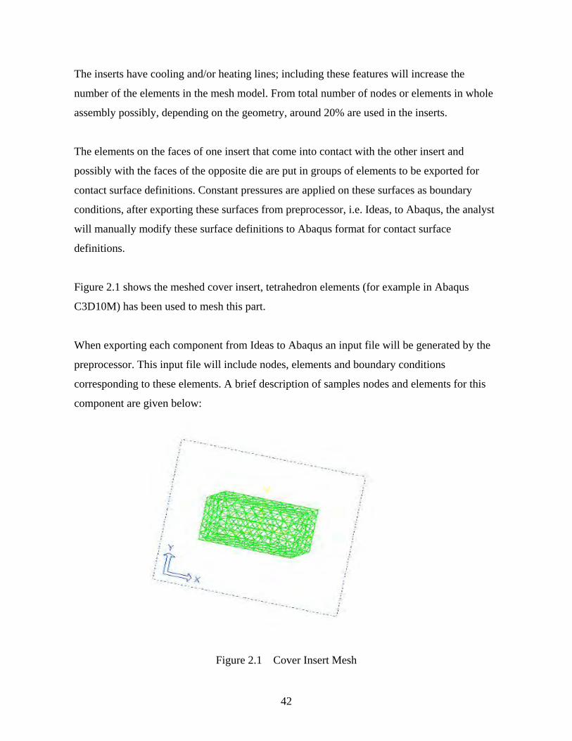
42
The inserts have cooling and/or heating lines; including these features will increase the
number of the elements in the mesh model. From total number of nodes or elements in whole
assembly possibly, depending on the geometry, around 20% are used in the inserts.
The elements on the faces of one insert that come into contact with the other insert and
possibly with the faces of the opposite die are put in groups of elements to be exported for
contact surface definitions. Constant pressures are applied on these surfaces as boundary
conditions, after exporting these surfaces from preprocessor, i.e. Ideas, to Abaqus, the analyst
will manually modify these surface definitions to Abaqus format for contact surface
definitions.
Figure 2.1 shows the meshed cover insert, tetrahedron elements (for example in Abaqus
C3D10M) has been used to mesh this part.
When exporting each component from Ideas to Abaqus an input file will be generated by the
preprocessor. This input file will include nodes, elements and boundary conditions
corresponding to these elements. A brief description of samples nodes and elements for this
component are given below:
Figure 2.1 Cover Insert Mesh

43
The following is a sample node set in Abaqus format: *** Node set NEINS *NODE, SYSTEM=R, NSET=NEINS 25001,-4.3771641E+02, 7.3565754E+02,-3.4694470E-15 25002,-4.3023860E+02, 7.3565754E+02,-3.4694470E-15 25003,-4.3023860E+02, 7.4289137E+02, 0.0000000E+00 25004,-4.3771641E+02, 7.3565754E+02,-4.4873333E+00 25005,-4.3023860E+02, 7.3565754E+02,-4.4873333E+00 25006,-4.3023860E+02, 7.4289137E+02,-4.4873333E+00 25007,-4.3771641E+02, 7.3565754E+02,-8.9746667E+00 Where in Abaqus:
* one star at first position of line indicates the command line.
** two or more stars at first position of line indicate comments.
*NODE this command indicates what is followed is the node definition.
SYSTEM= this command indicates what type coordinate system is used.
NSET= this command indicates the node name set, in this example the node name set
is NEINS, this name shows node for ejector insert
Each line after * NODE line shows the Node Number and its X, Y, Z coordinates in the
corresponding coordinate system selected and in the units of measurements selected in the
Ideas. In the above example, the first line after *NODE, is the node number 25001 having X
coordinate located at 4.3771641E+02, Y at 7.3565754E+02, and Z at -3.4694470E-15 in a
global Cartesian coordinate system and units of measurements is mm in this example.
A sample element set of the input file in Abaqus format is as follows: *ELEMENT,TYPE=C3D10M ,ELSET=EINS 1, 217, 121, 10, 120, 302, 129, 300, 301, 127, 131 2, 172, 73, 88, 71, 205, 103, 303, 206, 72, 240 3, 118, 19, 39, 41, 304, 271, 136, 135, 296, 40 4, 99, 69, 71, 226, 203, 70, 98, 305,

44
248, 242 5, 292, 7, 31, 251, 308, 32, 306, 307, 259, 258 6, 166, 226, 99, 287, 312, 305, 204, 311, 309, 310 *SOLID SECTION, ELSET = EINS, MATERIAL = 4140
*MAT, NAME = 4140
*ELASTIC, TYPE = ISOTROPIC
2.068E+05 2.900E-01
*DENSITY
7.820E-06
*EXPANSION, TYPE=ISO, ZERO=21.85
1.170E-05
*CONDUCTIVITY, TYPE=ISO
4.000E+01
Where in Abaqus format:
*ELEMENT this command indicates what is followed is the element definition.
TYPE= this option indicates type of element is used, in this case is 10 node modified
tetrahedron, C3D10M.
ELSET= this option indicates the element name set; in this example the element name
set is EEINS. All elements after *ELEMENT will be in this set until the next *ELEMENT is
encountered. This name shows elements for ejector inserts.
*SOLID SECTION this command indicates that the lines that will follow this command
are section properties of the element set, with specified element set and the material name. For
solid elements there is no next line. For plate elements the next line will indicate the thickness
of the plate. The arguments of these command ELSET= is the name of element set, and
MATERIAL= is the name of the material for this element set.

45
* MAT this command indicates, what will follow are the mechanical and or thermal
properties for the specified material. The argument, NAME= is the name given to this
material properties.
*ELASTIC command indicates that in the next line the elastic module and poisson ratio of
the material will be specified.
* DENSITY this statement indicates that in the next line the density of the material will be
specified.
*EXPANSION this command indicate that in the next line the expansion coefficient of
the material will be specified.
*CONDUCTIVITY this command indicates that in the next line the thermal conductivity of
the material will be specified.
TYPE= This option in the density, elastic, expansion, conductivity commands indicates
what type of material or thermal properties are defined, isotropic or anisotropic.
In above example, element 1, is a C3D10M ( three dimensional continuum element)
tetrahedron with 10 nodes and modified shape function, the node numbers are 217, 121, 10,
120, 302, 129, 300, 301, 127, 131, these nodes are defined in the node section. In this
example, the insert is made of 4140 steel. The *ELASTIC command show that for the inserts
a linear elastic and isotropic material property is used. The material properties are given as:
E=2.068E+5 N/mm*mm, Poisson ratio = 0.29. Also given the density and conductivity of the
material used in the simulation. Similar outputs will be generated for nodes and element sets
of cover insert, dies or other parts.

46
2.2.2Dies
A detailed geometry of dies, like inserts, should be incorporated into the analysis model. Dies
are meshed similar to the inserts. Therefore they will be meshed with a larger percent of total
elements. The dies have cooling / heating lines that will increase the number of the elements,
like inserts possibly, depending on the geometry, 20 % of the total elements will be used to
mesh dies. The element size is around 50 mm or less similar to insert mesh density. The
tetrahedron or hexahedron elements are used to mesh the dies. The elements on the faces one
die that come into contact with the opposite insert, support block, platen, and other die are put
in groups of elements to be exported for contact definitions, similar to inserts.
Figure 2.2 and Figure 2.3 show the cover die and ejector die meshes, tetrahedron elements are
used mesh their solid models ( for example in Abaqus C3D10M) . In these dies the locator
pins are located on the cover die, and they have been included in the cover die solid model.
The locator pins are meshed similar to the dies. The corresponding locator holes can be seen
on the ejector die mesh. The locator pins on the cover die comes into contact with the locator
holes in the ejector die. The elements on the surface of locator pins and elements on the
surface of locator holes are pit into sets to define the contact surfaces between the locator pins
and locator holes. The locator pins and holes should be always be included in the ejector and
cover dies models to prevent slipping of the ejector and cover dies relative to each other
during the loading.

47
Figure 2..2 Cover Die Mesh Model
Figure 2.3 Ejector Die Mesh Model
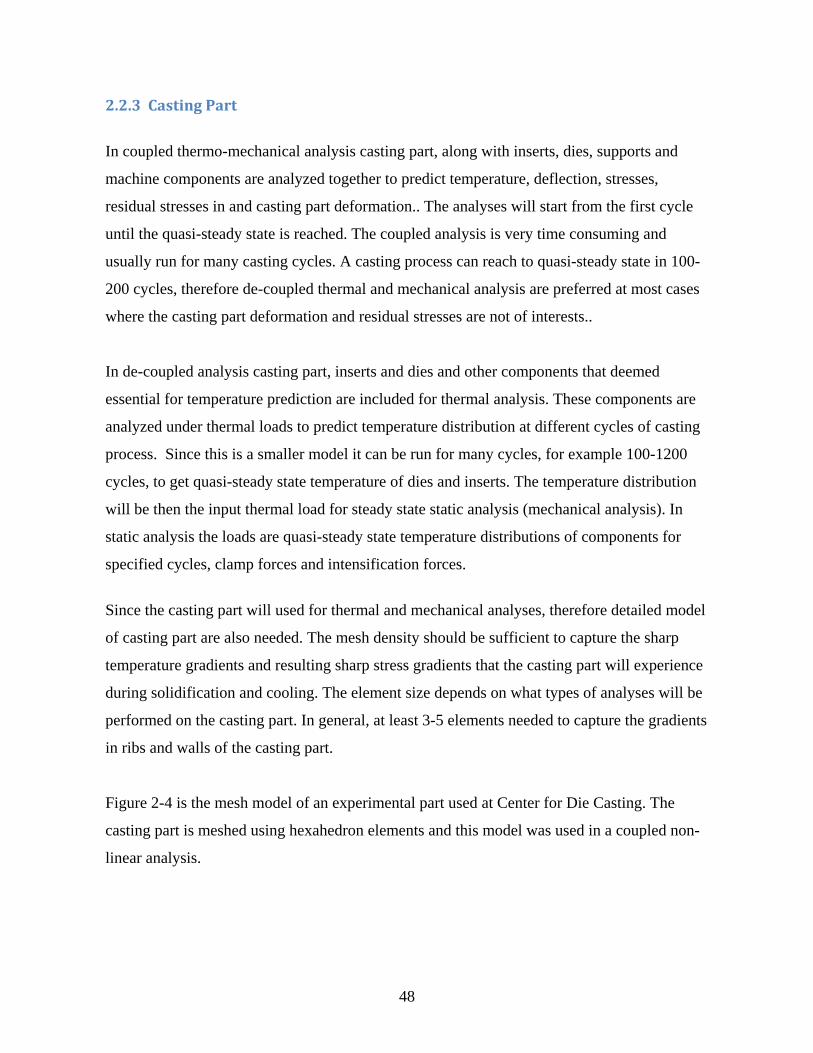
48
2.2.3CastingPart
In coupled thermo-mechanical analysis casting part, along with inserts, dies, supports and
machine components are analyzed together to predict temperature, deflection, stresses,
residual stresses in and casting part deformation.. The analyses will start from the first cycle
until the quasi-steady state is reached. The coupled analysis is very time consuming and
usually run for many casting cycles. A casting process can reach to quasi-steady state in 100-
200 cycles, therefore de-coupled thermal and mechanical analysis are preferred at most cases
where the casting part deformation and residual stresses are not of interests..
In de-coupled analysis casting part, inserts and dies and other components that deemed
essential for temperature prediction are included for thermal analysis. These components are
analyzed under thermal loads to predict temperature distribution at different cycles of casting
process. Since this is a smaller model it can be run for many cycles, for example 100-1200
cycles, to get quasi-steady state temperature of dies and inserts. The temperature distribution
will be then the input thermal load for steady state static analysis (mechanical analysis). In
static analysis the loads are quasi-steady state temperature distributions of components for
specified cycles, clamp forces and intensification forces.
Since the casting part will used for thermal and mechanical analyses, therefore detailed model
of casting part are also needed. The mesh density should be sufficient to capture the sharp
temperature gradients and resulting sharp stress gradients that the casting part will experience
during solidification and cooling. The element size depends on what types of analyses will be
performed on the casting part. In general, at least 3-5 elements needed to capture the gradients
in ribs and walls of the casting part.
Figure 2-4 is the mesh model of an experimental part used at Center for Die Casting. The
casting part is meshed using hexahedron elements and this model was used in a coupled non-
linear analysis.
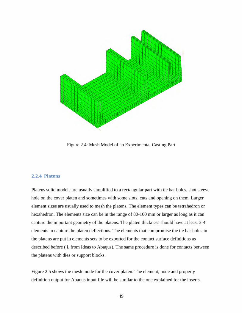
49
Figure 2.4: Mesh Model of an Experimental Casting Part
2.2.4Platens
Platens solid models are usually simplified to a rectangular part with tie bar holes, shot sleeve
hole on the cover platen and sometimes with some slots, cuts and opening on them. Larger
element sizes are usually used to mesh the platens. The element types can be tetrahedron or
hexahedron. The elements size can be in the range of 80-100 mm or larger as long as it can
capture the important geometry of the platens. The platen thickness should have at least 3-4
elements to capture the platen deflections. The elements that compromise the tie bar holes in
the platens are put in elements sets to be exported for the contact surface definitions as
described before ( i. from Ideas to Abaqus). The same procedure is done for contacts between
the platens with dies or support blocks.
Figure 2.5 shows the mesh mode for the cover platen. The element, node and property
definition output for Abaqus input file will be similar to the one explained for the inserts.

50
Figure 2.5: Cover Platen Mesh Model
2.2.5TieBars
Tie bars can be meshed using three dimensional solid elements or beam elements. If tie bars
are modeled using solid volumes, cylindrical objects, in solid modeling they are meshed using
solid elements of tetrahedrons o hexahedrons types. The element size for theses three
dimensional elements are around 80-100 mm. The element size is selected such that there will
be at least 4-5 elements along the diameter of the tie bars. AS mentioned in modeling sections
of tie bars, it is a g0od practice to partition to different segments to have provisions for
contact definitions with the platens. The portions of surface of elements of each tie bar that
comes into contact with ejector platen, cover platen and rear platen are put into a different
element sets for contact surface definitions with appropriate platen. Figure 2-6 shows the solid
model mesh of the tie bars using Tetrahedron elements (for example in Abaqus C3D10M). In
general it is easer to make volume solid models of the tie bars and platens and define the
contacts between or among them.
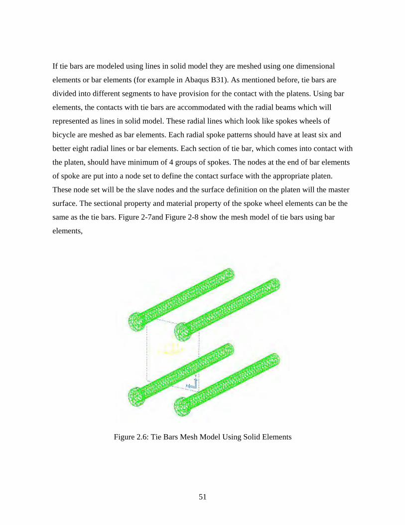
51
If tie bars are modeled using lines in solid model they are meshed using one dimensional
elements or bar elements (for example in Abaqus B31). As mentioned before, tie bars are
divided into different segments to have provision for the contact with the platens. Using bar
elements, the contacts with tie bars are accommodated with the radial beams which will
represented as lines in solid model. These radial lines which look like spokes wheels of
bicycle are meshed as bar elements. Each radial spoke patterns should have at least six and
better eight radial lines or bar elements. Each section of tie bar, which comes into contact with
the platen, should have minimum of 4 groups of spokes. The nodes at the end of bar elements
of spoke are put into a node set to define the contact surface with the appropriate platen.
These node set will be the slave nodes and the surface definition on the platen will the master
surface. The sectional property and material property of the spoke wheel elements can be the
same as the tie bars. Figure 2-7and Figure 2-8 show the mesh model of tie bars using bar
elements,
Figure 2.6: Tie Bars Mesh Model Using Solid Elements
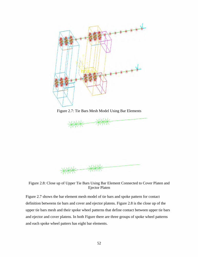
52
Figure 2.7: Tie Bars Mesh Model Using Bar Elements
Figure 2.8: Close up of Upper Tie Bars Using Bar Element Connected to Cover Platen and Ejector Platen
Figure 2.7 shows the bar element mesh model of tie bars and spoke pattern for contact
definition betweens tie bars and cover and ejector platens. Figure 2.8 is the close up of the
upper tie bars mesh and their spoke wheel patterns that define contact between upper tie bars
and ejector and cover platens. In both Figure there are three groups of spoke wheel patterns
and each spoke wheel patters has eight bar elements.
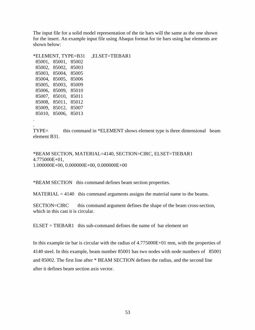
53
The input file for a solid model representation of the tie bars will the same as the one shown for the insert. An example input file using Abaqus format for tie bars using bar elements are shown below: *ELEMENT, TYPE=B31 ,ELSET=TIEBAR1 85001, 85001, 85002 85002, 85002, 85003 85003, 85004, 85005 85004, 85005, 85006 85005, 85003, 85009 85006, 85009, 85010 85007, 85010, 85011 85008, 85011, 85012 85009, 85012, 85007 85010, 85006, 85013 . . TYPE= this command in *ELEMENT shows element type is three dimensional beam element B31. *BEAM SECTION, MATERIAL=4140, SECTION=CIRC, ELSET=TIEBAR1 4.775000E+01, 1.000000E+00, 0.000000E+00, 0.000000E+00 *BEAM SECTION this command defines beam section properties. MATERIAL = 4140 this command arguments assigns the material name to the beams. SECTION=CIRC this command argument defines the shape of the beam cross-section, which in this cast it is circular.
ELSET = TIEBAR1 this sub-command defines the name of bar element set
In this example tie bar is circular with the radius of 4.775000E+01 mm, with the properties of
4140 steel. In this example, beam number 85001 has two nodes with node numbers of 85001
and 85002. The first line after * BEAM SECTION defines the radius, and the second line
after it defines beam section axis vector.

54
2.2.6ToggleMechanism
Toggle mechanism can be meshed using bar elements or solid elements. Toggle mechanism is
connected at one end to cover platen and the other end connected to rear platen. If rear platen
is not modeled in die and machine assembly then the toggle mechanism is modeled or meshed
as spring elements.
If rear platen is a part of the assembly the toggle mechanism can be modeled using lines to be
meshed as beam/bar elements or as cylindrical volume shapes to be meshed using three
dimensional elements like tetrahedrons or hexahedrons elements. In order to define the
diameter of the bar elements or model them as cylindrical shapes the equivalent stiffness of
toggle mechanism should be calculated. These procedures were explained in section 1.4.3.8.
Toggle mechanism models should represent closely actual set up in the die machine. In order
toggle mechanisms models distribute the forces more uniformly on the platens the equivalent
stiffness model of the upper and lower toggles should be divided among at least 4 or five
beams or cylinders respectively. Figure 2.9 shows the ejector platen, rear platen and toggle
mechanisms solid models. In this model toggles are represented by equivalent beam elements,
and inn this case the equivalent stiffness of the upper and lower toggle has been divided
among 4 beams.
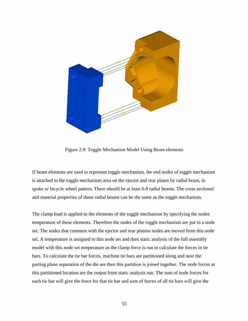
55
Figure 2.9: Toggle Mechanism Model Using Beam elements
If beam elements are used to represent toggle mechanism, the end nodes of toggle mechanism
is attached to the toggle mechanism area on the ejector and rear platen by radial beam, in
spoke or bicycle wheel pattern. There should be at least 6-8 radial beams. The cross sectional
and material properties of these radial beams can be the same as the toggle mechanism.
The clamp load is applied to the elements of the toggle mechanism by specifying the nodes
temperature of these elements. Therefore the nodes of the toggle mechanism are put in a node
set. The nodes that common with the ejector and rear platens nodes are moved from this node
set. A temperature is assigned to this node set and then static analysis of the full assembly
model with this node set temperature as the clamp force is run to calculate the forces in tie
bars. To calculate the tie bar forces, machine tie bars are partitioned along and near the
parting plane separation of the die are then this partition is joined together. The node forces at
this partitioned location are the output from static analysis run. The sum of node forces for
each tie bar will give the force for that tie bar and sum of forces of all tie bars will give the
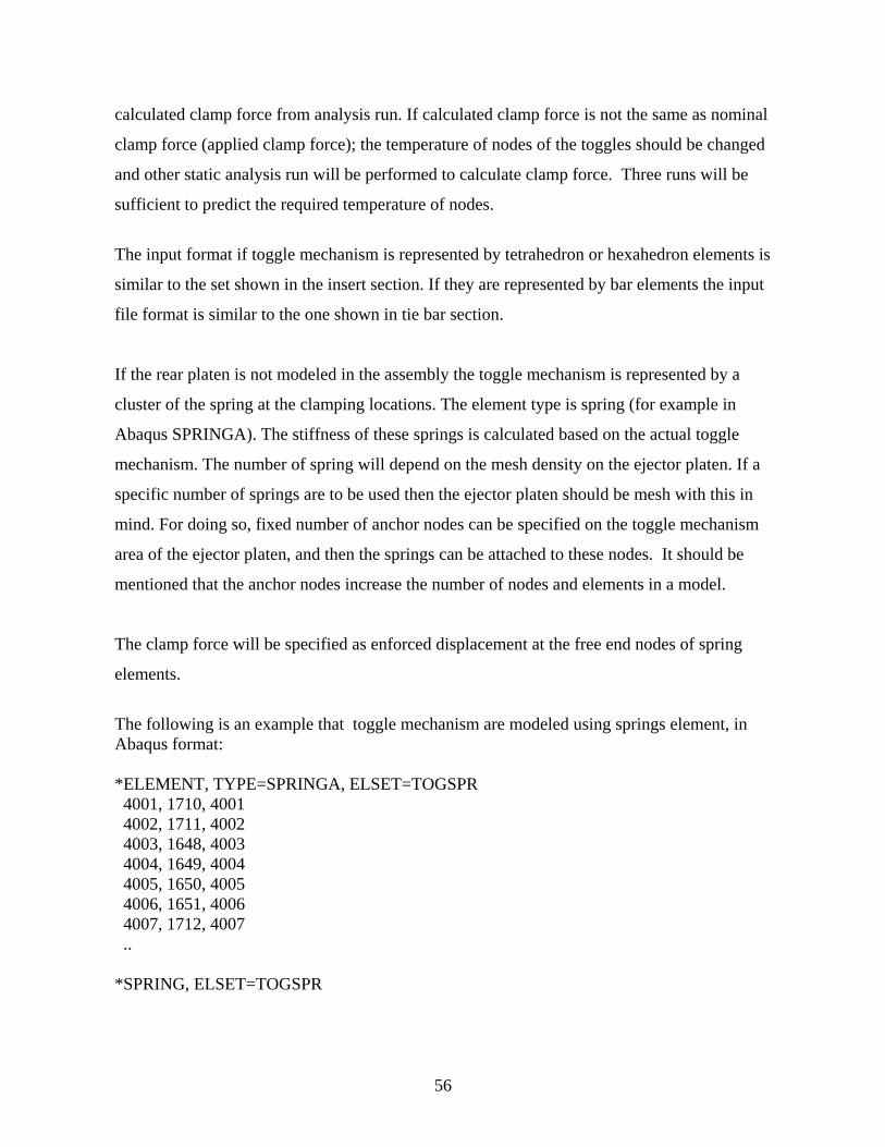
56
calculated clamp force from analysis run. If calculated clamp force is not the same as nominal
clamp force (applied clamp force); the temperature of nodes of the toggles should be changed
and other static analysis run will be performed to calculate clamp force. Three runs will be
sufficient to predict the required temperature of nodes.
The input format if toggle mechanism is represented by tetrahedron or hexahedron elements is
similar to the set shown in the insert section. If they are represented by bar elements the input
file format is similar to the one shown in tie bar section.
If the rear platen is not modeled in the assembly the toggle mechanism is represented by a
cluster of the spring at the clamping locations. The element type is spring (for example in
Abaqus SPRINGA). The stiffness of these springs is calculated based on the actual toggle
mechanism. The number of spring will depend on the mesh density on the ejector platen. If a
specific number of springs are to be used then the ejector platen should be mesh with this in
mind. For doing so, fixed number of anchor nodes can be specified on the toggle mechanism
area of the ejector platen, and then the springs can be attached to these nodes. It should be
mentioned that the anchor nodes increase the number of nodes and elements in a model.
The clamp force will be specified as enforced displacement at the free end nodes of spring
elements.
The following is an example that toggle mechanism are modeled using springs element, in Abaqus format: *ELEMENT, TYPE=SPRINGA, ELSET=TOGSPR 4001, 1710, 4001 4002, 1711, 4002 4003, 1648, 4003 4004, 1649, 4004 4005, 1650, 4005 4006, 1651, 4006 4007, 1712, 4007 .. *SPRING, ELSET=TOGSPR

57
5.8806E+04 TYPE= this sub-command or option defines the element type, in this example element type is SPRINGA ELSET= this option defines the name of element set. *SPRING this command will give the spring stiffness along the two nodes. In the above example 4001 is a SPRINGA element, and it is numbered 4001, with two node
numbers 1701, and 4001. These nodes are defined in the node section of the input file. The
first line after *SPRING command is a blank line for the SPRINGA, the second line is the
stiffness of the spring.
2.2.7SupportBlocks,BackPlatesandPillars
The support blocks and back plates mesh density and element size can be similar to the
platens mesh and density. These parts can be meshed using tetrahedron or hexahedron
elements (for example using C3D10M elements in Abaqus). These parts usually have box
shape geometry with some pillars and some ejector pin holes; therefore it may require a more
detailed solid model and with more mesh density than the platens. The analysts should decide
how much detail is required for the type of computer simulation is considering to be analyzed.
In general ejector pin holes can be neglected but the pillars are very important in load path
and therefore in load distribution and die deflections. The pillars should always be a part of
the solid model and meshed assembly.
The surface of elements on one face support blocks and back plates come into contact with
the ejector platen, and on the other face come into contact with the die. The elements on each
face are put in a separate element set for contact surface definition (see section 3.1.8).
Figure 2.10 shows the model of the ejector die, ejector plate along with the back frame/
support block. In this model there are no support pillars, but the model has the guiding pine
for the ejector plate.

58
Figure 2.10: Ejector Back Plate, Back Frame and Ejector Die
2.2.8DieCastingMachineBase
A simplified solid model of the machine base should be constructed and be included in the die
and machine assembly. Figure 1.17 shows the die and machine assembly solid model. The
machine base is meshed using three dimensional elements, tetrahedron and hexahedron
elements. The machine base is included in the total machine assembly for two reasons:
1) In some die machines the cover platen attached to the machine base by welding bottom
edges of the platen to the base and in other machines the cover platen bottom is joined to the
base by bolts. For the case of welded joints; the nodes on the perimeter of the cover platen can
be tied to the machine base nodes. For the case the bolted joint; this joint can be represented
either by using tied nodes where nodes on the machine base and cover platen are tied together
or bolts can be explicitly modeled using beam elements where these beam elements are
attached at one end the cover platen and on the other end to the machine base.

59
2) The ejector platen and rear platen slide on the machine base, and they could move upward
and get detached from the base, but they can not move downward. The railing of the machine
base will make it possible to achieve both proposes by defining the contact conditions
between the machine base railings and bottom of ejector and rear platens.
The attachment or joint between the bottom of cover platen and the top of machine base is
defined using boundary condition of the solvers.
Pictures in Figure 2.11 show the mesh model of the machine assembly and various boundary
conditions used to define the joints attachments between the cover platen and machine base. .
In This figure the mesh model of cover, ejector and rear platens along with toggle mechanism,
tie bars and machine base mesh are shown. Also shows in these figures three ways that
analyst could select based on the machine type to attach the cover platens to the machine base.
Figure 2.11-a shows the case where platen bottom edge are welded to the base, in this case the
bottom edge nodes of platen are tied to the corresponding nodes of the machine base, this type
of connection will represent welded edges. If the bottom of the cover platen are bolted to the
machine base with many bolts this model can be represented by tying all nodes on the bottom
of the cover platen to the nodes on the machine base, this model is shown in Figure 2.11-b. If
bottom of the cover platen is attached to the machine base by few bolts and the analyst is
interested in bolts pre-loads and bolts stretching during the die casting processes and loading
conditions, then these bolts can be modeled explicitly. Figure 2.11-c shows the model when
the cover plated is bolted to the machine base, this figure is the close dup of the bolt model
and how they are attached to the cover platen and machine base. As can be seen from the
Figure 2.11-c six bolts joins the cover platen to the base, beam elements are used to represent
the bolts. One end of beams are attached to the cover platen and the other end is attached to
the machine base using spoke pattern or bicycle wheel shape. The spoke pattern will distribute
the forces more uniformly among more nodes on the cover platen and machine base and
prevent excess deformation die to one node connection.
If machine base is not molded explicitly then the machine railing, which ejector and rear
platens slide on it, should be included in the machine assembly. This motion of the ejector and

60
rear platen on the railing is defined using contact conditions. The contact conditions can be
achieved by using rigid surfaces; in this case the interaction between the rigid surface and the
bottom surfaces of the ejector and rear platens should be defined. For this case the cover
platen nodes are constrained in all directions to prevent it from moving.
For example in Abaqus, the sliding plane, which the ejector and rear platens ride on it, will be
meshed using rigid elements R3D3. A node that is associated with this rigid element set is
anchored not to move, this node’s all degrees of freedoms will be constrained.

61
Figure 2.11: Boundary Conditions used Between Cover Platen and Base
2.2.9DieSlides
The die slides is meshed similar to dies and inserts using three dimensional solid elements like
tetrahedron or hexahedron elements. The element size and the mesh density will be similar to
the inserts. Care should be taken for the contact conditions between the die slides and the dies

62
or inserts. The mesh density should be fine enough to capture the contact interaction between
or among them. The contact conditions are defines using contact surfaces similar to others
contact conditions.
2.2.10OtherUn‐commonComponentsofMachineorDies
Some die designs can have additional parts to enable them to be mounted on different die
casting machines. For example, when mounting smaller dies on larger die casting machine
the die height of the die should be increased to do so additional components designed to be
attached to the cover or ejector dies backsides. These un-common components can play an
impotent roll in load pass and load distribution on the die faces, therefore on parting plane
separation of the dies. It is very important that analyst include these parts they way were
intended to function.. These parts can be meshed with the similar element type and mesh
density as platens or dies depending on their functionality o and how they are assembled
relative to the neighboring parts. The mesh density of these parts should reflect the role they
play during die casting process for re-distributing the loads and how they affect the load path.
2.2.11TieBarsNuts
Tie bar nuts can be meshed using two dimensional plate elements (for example in Abaqus
S3R a 3 node element or STR65 a 6 node element) or using three dimension solid elements
like tetrahedron or hexahedron elements.
If plate elements are used a thickness will be assigned to these elements which is equal to the
nut thickness. The outer perimeters of these plate elements have common nodes with the
cover platen. The end of the tie bars which passes through cover platen holes are attached to
these nuts. If bar elements is used to model the tie bars, these beam elements will be attached
to the center node of the nut elements. This center node is also attached by spoke wheel
pattern using bar elements to the perimeter nodes of the nuts. If the inside nodes of the nuts
elements are tied to the platen nodes then the spoke pattern bar elements are not needed.

63
If the nuts are modeled using solid elements; the inside nodes on these nuts elements are
attached or tied to the outer nodes of the tie bars, where they come into contact. In effect the
nuts can be a part of the tie bar model, see Figure 2.6. The nuts also can have common nodes
on the face of the nuts where they comes into contact with the cover platen, or these nodes on
the nuts can have contact condition with the cover platen.
Figure 2.6 shows the mesh model of the tie bars and nuts using tetrahedron elements. In
Figures 2-7 and Figure 2-8 there is no nut model, but the tie bars are connected to the cover
platen through the spoke wheel bar elements.
2.2.12BoltJointsBetweenComponents
The bolt joints between any two parts or components can be represented by beam (bars)
elements or by tied nodes.
The beam/bar representation is more realistic but will increase the complexity of the solid
model construction also it will increase the number of nodes and elements drastically. In this
case, the bolt holes will be explicitly molded in corresponding parts. To model a bolt, a bar or
beam element is constructed equal to the length of the bolt, then the node on each end of this
beam element is attached to the corresponding parts through a spoke wheel pattern using
additional bar or beam elements. The material and cross sectional properties of the beam
representing the bolt and the spoke wheel bars will be similar to the bolt itself.
The following is a sample input file for a bolt model in Abaqus format *ELEMENT,TYPE=B31 ,ELSET=CBOLT1 80001, 80001, 80002 . . * cbolt-ci-b1 80009, 80001, 50013 80010, 80001, 50015 80011, 80001, 50028 80012, 80001, 50035
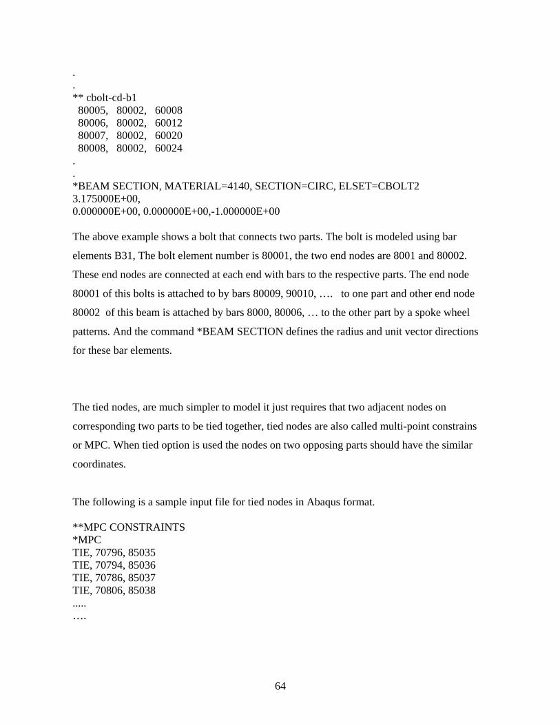
64
.
. ** cbolt-cd-b1 80005, 80002, 60008 80006, 80002, 60012 80007, 80002, 60020 80008, 80002, 60024 . . *BEAM SECTION, MATERIAL=4140, SECTION=CIRC, ELSET=CBOLT2 3.175000E+00, 0.000000E+00, 0.000000E+00,-1.000000E+00 The above example shows a bolt that connects two parts. The bolt is modeled using bar
elements B31, The bolt element number is 80001, the two end nodes are 8001 and 80002.
These end nodes are connected at each end with bars to the respective parts. The end node
80001 of this bolts is attached to by bars 80009, 90010, …. to one part and other end node
80002 of this beam is attached by bars 8000, 80006, … to the other part by a spoke wheel
patterns. And the command *BEAM SECTION defines the radius and unit vector directions
for these bar elements.
The tied nodes, are much simpler to model it just requires that two adjacent nodes on
corresponding two parts to be tied together, tied nodes are also called multi-point constrains
or MPC. When tied option is used the nodes on two opposing parts should have the similar
coordinates.
The following is a sample input file for tied nodes in Abaqus format. **MPC CONSTRAINTS *MPC TIE, 70796, 85035 TIE, 70794, 85036 TIE, 70786, 85037 TIE, 70806, 85038 ..... ….

65
The above example shows that the nodes 70796 and 85035 are tied to together, each node is
located at two adjacent parts.
Figure 2.11 shows different joints modes. Figures 2.11-a and 2.11-b are the models for the
weld joints or bolt joints using tied nodes or multi-point constrains, and Figure 2.11-c shows
explicit bolts models using beam elements.
3. Boundary Conditions and Material Properties
The computer simulation of the dies and die machine is completed by the additions of the
boundary conditions. The boundary conditions include thermal and mechanical loads,
constrains and interaction between and among the components. Also the material properties
which include physical, mechanical and thermal properties should be defined for each
component in the model assembly based on the type of analysis will be performed to simulate
the die casting processes.
3.1MechanicalLoads
The mechanical loads in a die casting simulations can include;
A) Enforced displacements to represent the clamp forces when spring element is used to
model the toggle mechanisms.
B) Distributed pressure load on the toggle mechanism area to represent the clamp load when
toggle mechanism is not included in the simulation model. Case A and case B clamp forces
models will ignore the change in clamp force during the machine operation.
C) Intensification pressure is modeled using distributed pressure loading on the inner surface
of inserts, part cavity, and outer surface of the casting part.
Some solvers have special elements that can transfer hydrostatic loads. If these special
elements are used for the casting part, then these elements can transfer hydrostatic pressure
though the contact between the insert and casting part to the insert cavity, then intensification
pressure should be applied only on the surface area of biscuit.

66
3.2ComponentsConstraints
Components constraints are the boundary conditions in the simulations which have to be
defined. The boundary conditions specified in die casting simulations should represent the
actual constraints since they play a great role in defining how the simulation assembly will
behave. Therefore a great deal of attention should be paid to define the assembly constraints
with proper simulation boundary conditions.
3.2.1TieBarConstraints
If rear platen is not included in the machine model assembly and tie bars are meshed using
solid / brick (i.e. in Abaqus C3D10M) elements, then all degrees of the freedoms (X, Y and Z
in Abaqus 1, 2, and, 3) are constrained at the open end of tie bars and the other end of tie bars
are attached to the cover platen as explained before. If tie bars are meshed using bar
elements (i.e. in Abaqus B31) elements, all degrees of the freedom (X, Y,Z, ROTX, ROTY,
and ROTZ, or in Abaqus 1, 2, 3, 4, 5 and 6) are constrained at the open end.
If the rear platen model is included in the machine model assembly one end of tie bars
attached to the cover platen and the other end of tie bars attached to the rear platen as
previously described.
An Abauqs input file for boundary conditions examples is defined bellow:
*BOUNDARY, OP=NEW 85021, 1, 6, 0.00000E+00 85022, 1, 6, 0.00000E+00 85022, 1, 3, 0.00000E+00 . . The constraint command beings with *BOUNDARY, the parameter OP or option will have
the choice of NEW or MOD. NEW for a new set of constraints or MOD to change the
constraints from the previous *SETP of analysis

67
In the above example the nodes 85021 and 85022 are constrained in all six directions or all six
degrees of freedom (1, 2, 3, 4, 5, and 6) have been constrained and node 52023 is constrained
in 1, 2 and 3 directions.
3.2.2EjectorandRearPlatensConstraints
The ejector and rear platens are constrained by the tie bars and the machine base to slide on
the railing of the machine base. The ejector and rear platens can separate from the base but
they can not penetrate into the machine base. These constrains are provided by using contact
surfaces between the platens and the railing.
3.2.3CoverPatenConstraints
If the machine base is not included in machine model assembly then the cover platen base is
constrained from moving up and side-ways at the four, six or more locations. It is sufficient to
constrain few nodes on the base of the cover platen, preferably these nodes will be at the
locations where the cover platen are bolted or welded to the base or frame of the die machine.
At the Center for Die Casting when modeling die casting machine the Z (i.e. 3 in Abaqus)
coordinate is parallel to the axes of tie bars, X (i.e. 1 in Abaqus ) coordinate and Y (i.e. 2 in
Abaqus) coordinate show lateral and vertical directions respectively. In Abaqus input file; in
this case the movement of the cover platen is constrained in lateral (i.e.1) and vertical
direction (i.e. 2)
An Example of Abaqus input file: *BOUNDARY, OP=NEW CVRPLT, 1, 2, 0.00000E+00 *NSET, NSET=CVRPLT 4021, 4022, 4023, 4024, 4025, 4026, 4027,4027 4122,4123,4124,4125

68
The node set CVRPLT which contained the nodes on the base of the cover platen is constrained in 1 (X) and 2 (Y) directions. If machine base is included in the machine model assembly the type of attachment can be
determined from the machine models as described in Chapter 2.
3.2.4ToggleMechanismUsingSprings
The case where toggle mechanism is molded using spring elements, one end of springs
elements are attached to the area on the ejector platen and the other end of springs elements
are free. The free ends of spring elements are constrained in all directions, except along the tie
bar axis (Z-direction). Along this axes (Z-direction) an enforced displacement boundary is
specified..
This magnitude of the enforced displacement is calculated from the relation
F=N*K*d
Where: F = Total force applied, N = Number of toggle springs, K = Toggle spring stiffness, D = Enforce displacement. The equivalent toggle stiffness, K, can be calculated as described in Chapter 1. Abaqus input file example:
The following input data show that the node set REAR-TOG of the toggle springs is given an
enforced displacement of –1.9 mm, in 3 ( Z) direction.
*BOUNDARY, OP=NEW REAR-TOG, 3,, -1.90000E+00 *NSET,NSET=REAR-TOG 4001, 4002, 4003, 4004, 4005, 4006, 4007, 4008, 4009, 4010, 4011 4012, 4013, 4014, 4015,.......

69
3.2.5SpringForcesontheDieSlides
The spring forces on the slides can be applied using spring elements (for example SPRING1
elements in Abaqus). The enforced displacements will be applied to the springs on slides to
be equal to the forces in the specified directions. The forces in three directions can be applied
using three springs in three different directions. The procedures and commands will be similar
to the toggle springs
3.2.6CastingPartandDies/InsertsPartCavityIntensificationPressure
In general, two kind of simulations models are used to model die casting process with given
mechanical and thermal loads and boundary conditions. One with the casting part included in
the die and machine assembly model and other one without the casting part. The latter is more
common practice and gives simpler models to run. The casting part is this case included only
for the thermal analysis in order to calculate the components transient or quasi-steady state
temperatures.
If the software solver has special elements that can transfer properly hydrostatic pressures,
then the part can be included in die and machine assembly model. In this case the
intensification pressure is described as a uniform distributed load on the surface of the biscuit.
At present the solvers that have proper hydrostatic elements they lack the proper calculation
of the deflections and stresses of elements. On the other hand there are solvers that their
hydrostatic elements behaves like forging elements, this mean that they can not properly
handle the liquid to solid transition during the die casting process (the casting parts separates
from the cavity) but they can correctly calculate the deflections and stresses of elements.
If the casting part is not included in the die and machine assembly model, the intensification
pressure is applied to the surface of the surface elements that make up the part cavity.
Intensification pressure is applied as a uniform distributed load.

70
The following is an Abaqus Input file that describes the intensification pressure on the part
cavity surface.
*DLOAD,OP=NEW CINS015, P1, 4.1364E+01 CINS016, P2, 4.1364E+01 CINS017, P3, 4.1364E+01 . *ELSET,ELSET=CINS015 40008,40068,40080,40092,40135,40139,40282,40539,40547,40599,40763,41027 41191,41283,41443,41575,41808,42040,42056,42120,42124,42298,42424,42426 42533,42596,42732,42772,42844 ELSET,ELSET=CINS016
5672.5682, 5890,5895,5960,59,65,5983,5988,5990
6005,6008,6011,6022,6026,...
...
*ELSET,ELSET=CINS016
7929, 7938,7955, 7820,......
…
The distributed loads are defined using *DLOAD commands in Abaqus , with the OP the
option parameter. The values of OP parameter are NEW or MOD. The NEW option is
specified when a new load on the load step is (*STEP) used and the MOD option is used
when the load will be modified from the previous load step (*STEP). The distributed loads
are applied on face of tetrahedron (four faces) or hexahedron (six faces) elements with to face
number assigned as P1 , P2, . .. and shell elements will have positive or negative directions.
In the above example intensification load has been applied to the insert cavity as a distributed
load on the element sets CINS015, CINS016 and CINS017. They are applied on the face 1
and 2 and 3 of the elements on the element sets CINS015, CINS016 and CINS017
respectively the magnitude of pressure is 4.13E01 N/mm2.
71
3.3TemperatureCalculations
In die casting before first casting starts, the die casters preheat the dies and insets to a
specified temperature for better casting operations. After the casting start from the time first
part is made; the dies and inserts temperatures will change with time. The spraying of the dies
and inserts are done after each casting cycle. The spaying will cool the dies and inserts
temperatures to prevent them from over heating. The increase in temperatures of dies and
inserts will results in their thermal growth and induce additional deflections of dies and inserts
besides deflections due to mechanical loads. Therefore a thermal analysis is an integrated part
of any die casting simulation with appropriate boundary conditions and proper thermal and
physical properties.
For thermal analysis a separate model is usually run which is consist of casting part, dies,
inserts and other components which deemed necessary during the thermal
3.3.1CastingPart,DiesandInsertsPartCavityHeattransferCoefficients
Heat transfer coefficients are assigned to the casting part surface and the part cavity. The
magnitude these heat transfer coefficients ranges of 5000 to 10000 W/m*m*C in SI units.
These magnitudes show the heat transfer coefficient between the molten cast part and the part
cavity of dies and inserts.
The inserts and dies also come into contact with each other too. These surfaces compromise
the parting plane surface; therefore heat transfer coefficient between them should also be
specified. The contact heat transfer coefficient is in the range of 5000 W/m*m*C in SI units
when there is no gap (zero separation) between adjacent surfaces. The contact heat transfer
coefficient is also called gap conductance. An example will be given in the next section.
3.3.2OutsideDiesHeatTransferCoefficients
The heat transfer from the die to ambient temperature is specified using heat transfer
coefficients. This heat transfer from the dies to the ambient t temperature is by natural
convection mostly, and if there is any air movement it will be at very low speeds.

72
The ambient die temperature (Tabm ) is usually fixed, at about 30 C, The natural heat transfer
coefficient, h, to the ambient from the dies is in the order of 20 to 30 W/m*m*C (or 0.02 -
0.3 W/mm*mm* C). The contact heat transfer coefficients (gap conductance) between the
die-to-die and die-to-inserts are around 5000 W/m*m*C.
In Abaqus, The heat transfer coefficients are specified using *FILM command. With the OP
option as new, OP=NEW. Each line after the *FILM command line will specify the element
numbers or element sets, face number, ambient temperature and the heat transfer coefficient.
Following is an Abaqus example for input file:
*FILM, OP=NEW
** GENER-CONV
EDH06, F1, 3.0000E+01, 2.0000E-02
EDH07, F2, 3.0000E+01, 2.0000E-02
EDH08, F3, 3.0000E+01, 2.0000E-02
*ELSET, ELSET = EDH06 5019,5023,5115,5122,5227,5259,5335,5378,5382,5403,5443,5502,5527 5575,5592,5611,5615,5658,5686,5708,5719,5723,5759,5764,5768,5803 5886,5924,5928,5930,5936,5942,5972,5980,5982,6018,6055,6074,6120 6144,6175,6198,6202,6208,…… *ELSET,ELSET=EDH07 7142,7152,7168,7198,8023, …. … *ELSET, ELSET=EDH08 …..
The above example defines heat transfer coefficients on the F1 (face 1), F2 (face 2) and F3 (
face 3) faces of the element set EDH06, EDH07, and EDH08 respectively. The ambient
temperature is 30 C and h= 0.02W/mm*mm*K (in this unit the length in mm).

73
3.3.3ContactHeatTransferCoefficients
The heat transfers between adjacent surfaces are described using contact heat transfer
coefficient or gap conductance. The contact heat transfer is used to define the boundary
conditions between or among contacting surfaces that their temperature changes during the
simulation and they are also having mechanical contacts. The contact is said to be perfect if
there is no opening between the adjacent surfaces or gap distance remains at 0.00 m. If gap
opening starts to develop during the simulation then the gap distance will be greater than 0.00
m. If only thermal analysis are performed on contacting surfaces, theses contacting surfaces
will always remain in contact and no gap will be developed and the gap conductance will be
constant. But if coupled thermo-mechanical analysis is done due to thermal loads or
mechanical loads gaps can be developed between and among the contacting surfaces due to
deformation of the adjacent components.. In the case of developing gap, gap opening, the
contact heat transfer coefficient or gap conductance will decrease with increasing gap.
The following statement describes the gap conductance definition in Abaqus;
*GAP CONDUCTANCE 5000, 0.000 4500, 0.20E-6 4000, 0.35E-6 3500, 0.50E-6 …. …. 1500, 2.0E-6 1000, 4.0E-6 750, 12.0E-6 In this above example the gap conductance decreases as the gap width increase from 5000
W/m*m*k at 0.00 m gap to 750 W/m*m*k at 12.0 µm (12.0E-6 m)
3.3.4HeatRemovalDuringSpraying
Spraying the dies and insert surfaces will result in removing heat from and cooling dies and
inserts and also lubricating the contacting surfaces. The amount of heat extracted during the
spaying varies substantially according to dies, inserts and casting part size and the practice

74
and experience of the die castes. The heat extracted by spraying can range from 15% to 30%
of the total heat generated by the solidifying casting part. At Center for Die Casting a value of
15% to 20% heat removal is usually used. To calculate the heat fluxes values for the dies and
inserts the following procedures, equations 3.1 to 3.3, can be used;
Qs = ks* Q (3.1)
where:
Qs The heat removed by spray
ks The factor for percent heat remove ( e.g. 0.15 in our application)
Q Total Heat released from solidifying casting part
The total heat release from the casting part from initial injection temperature TI, to average
ejection temperature TE can be calculated using:
Q = ρl*Cpl*Vpart*(TI-TSd.) + ρl * Vpart *Lh +
ρs *Cps*Vpart*(TSLd-TAE) (3.2)
Where:
ρl Density of Liquid
ρs Density of solid
Cpl Specific heat of casting material at liquid phase
Cps Specific heat of casting material at solid phase
Vpart Volume of the casting Part
TI Initial Injection temperature
TSLd Solidus / liquidus temperature
TAE Average Ejection temperature of the part
Lh Latent heat of the solidification
The heat flux that will be specified on the dies and inserts surfaces can be calculated using:

75
Q” = Qs/ (tis-tsp)*ATot (3.3)
where:
Q” Heat flux from the each volume or section
ATot Total surface where exposed to spraying
tsi Time spraying initiated (start time)
tsp Time spray ended (stop time)
The heat flux will be specified on the dies and inserts where spaying are done.
3.3.4.1 HeatTransferbyHeatFlux
Once the heat fluxes has been calculated during spaying time, then the heat flux boundary
conditions can be specified for thermal analysis. The heat fluxes are assigned to the surfaces
of the solid or plate elements. Thermal analysis of die casting processes is transient; it starts
from the first cycle and will continue until the dies and inserts reach to quasi-steady state. The
quasi-steady states indicate that the dies and inserts temperature will fluctuate around almost a
mean steady temperature without this mean temperature increasing much. In thermal or
coupled thermo-mechanical analyses the heat fluxes or heat transfer coefficients can be
defined as constant or varying with time.
For example in Abaqus the heat fluxes are defined inside the *STEP command using
*DFLUX command with the parameters Op (option) and AMPLITUDE.
The OP parameter is similar to the ones in *DLOAD, and *BOUNDARY. The AMPLITUDE
parameter gives how the heat flux magnitude changes in this step. The AMPLITUDE is set
equal to the name of a curve that defines the magnitude change in this step.
The parameter AMPLITUDE is defined by the command *AMPLITUDE which has
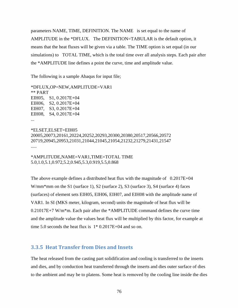
76
parameters NAME, TIME, DEFINITION. The NAME is set equal to the name of
AMPLITUDE in the *DFLUX. The DEFINITION=TABULAR is the default option, it
means that the heat fluxes will be given via a table. The TIME option is set equal (in our
simulations) to TOTAL TIME, which is the total time over all analysis steps. Each pair after
the *AMPLITUDE line defines a point the curve, time and amplitude value.
The following is a sample Abaqus for input file; *DFLUX,OP=NEW,AMPLITUDE=VAR1 ** PART EIH05, S1, 0.2017E+04 EIH06, S2, 0.2017E+04 EIH07, S3, 0.2017E+04 EIH08, S4, 0.2017E+04 ... *ELSET,ELSET=EIH05 20005,20073,20161,20224,20252,20293,20300,20380,20517,20566,20572 20719,20945,20953,21031,21044,21045,21054,21232,21279,21431,21547 ..... *AMPLITUDE,NAME=VAR1,TIME=TOTAL TIME 5.0,1.0,5.1,0.972,5.2,0.945,5.3,0.919,5.5,0.868 The above example defines a distributed heat flux with the magnitude of 0.2017E+04
W/mm*mm on the S1 (surface 1), S2 (surface 2), S3 (surface 3), S4 (surface 4) faces
(surfaces) of element sets EIH05, EIH06, EIH07, and EIH08 with the amplitude name of
VAR1. In SI (MKS meter, kilogram, second) units the magnitude of heat flux will be
0.21017E+7 W/m*m. Each pair after the *AMPLITUDE command defines the curve time
and the amplitude value the values heat flux will be multiplied by this factor, for example at
time 5.0 seconds the heat flux is 1* 0.2017E+04 and so on.
3.3.5HeatTransferfromDiesandInsetsThe heat released from the casting part solidification and cooling is transferred to the inserts
and dies, and by conduction heat transferred through the inserts and dies outer surface of dies
to the ambient and may be to platens. Some heat is removed by the cooling line inside the dies

77
and inserts. The heat transfer from inserts to dies are defined using contact heat transfer or gap
conductance, and the heat transfer from dies to the ambient temperature is specified by using
the natural heat transfer coefficients between the dies and ambient. The procedures for
defining heat transfer coefficients are described in section 3.3.2.
3.3.6CoolingandHeatingLinesHeatTransfer
The dies and inserts are designed to work the best while their temperatures are controlled
within the desired operating temperatures. The cooling and heating lines are used to achieve
this goal. The cooling lines will remove excess heat form dies and inserts and lower their
temperatures. The heating lines are used to add heat to the areas of ides and inserts where the
temperature is low.
The cooling and heating lines heat transfer coefficients are specified using heat transfer
coefficients commands (for example in Abaqus using *FILM command). This is similar to
die heat transfer coefficient definition in section 3.3.2. The magnitude of the heat transfer
coefficient is much larger than natural heat transfer coefficient to ambient. The cooling and
heating line heat transfer coefficients are around 5000 W/m*m*C.
For cooling line; the ambient temperature, for recirculation media which is usually water, is
usually given to be around 30C.
For cooling line; the ambient temperature, for recirculation media which is usually oil, will
depend on the operating condition of die casting and should be specified by the design
engineers and it can be in the range of 150-200C.
3.4ContactSurfaces
Contact surface definitions are used to define the mechanical interaction and or heat transfer
between two contacting surfaces.
The mechanical contact between two surfaces can be defined by assigning Coulomb friction
coefficients to these surfaces. If this coefficient is zero the contact surfaces are said to be

78
frictionless. The contact heat transfer (gap conductance) is used when heat is transferred
between to adjacent surfaces with a given heat transfer coefficients when temperature of both
surfaces change during the simulations.
In some pre-processors the contact surfaces cannot be defined explicitly (like Ideas), therefore
the contacts between any two surfaces has to defined indirectly and sometimes manually
modifying the output surfaces from the pre-processor format to the solver format. The
surface definition in modeling and analysis means a collection of faces of adjacent elements.
Contact surfaces in Abaqus are defined by:
*SURFACE DEFINITION,NAME = Name-of -surface
Each lines after this command will give the element number or the set name, the face number
for the solid element or POS or NEG for shell elements that together define the surface name,
NAME= is used to assign a name to surface definition (Name-of –surface)
3.4.1ContactElementSetDefinition
To define the contact element sets definitions, the analyst will collect the faces of the
elements that will make the target surfaces of interests in one group.
For example in Ideas follow these steps.
1) Apply a pressure to the faces of elements that will be in contact with another surface with a
given pressure magnitude.
2) When these pressure boundaries exported from Ideas to Abaqus, Ideas will put these
elements in element sets, with given specific names
3) In load step there will be a pressure load with the name of each element set and the face
number, and the given pressure magnitude
4) Delete the pressure magnitude and convert it to a surface definition
Example of element sets with pressure on them:

79
*DLOAD,OP=NEW *** CINS-ci1 CDIE005, P4, 4.00E+01 CDIE004, P3, 4.00E+01 CDIE002, P1, 4.00E+01 CDIE003, P2, 4.00E+01 .... *DLOAD,OP=NEW *** CINS-cd1 CINS011, P1, 4.00E+01 CINS012, P2, 4.00E+01 CINS013, P3, 4.00E+01 CINS014, P4, 4.00E+01 ... The above element pressures on the element sets are converted to surface definitions. *SURFACE DEFINITION,NAME=CINS-ci1 CDIE002, S1 CDIE003, S2 CDIE004, S3 CDIE005, S4 ..... *SURFACE DEFINITION,NAME=EINS-cd1 CINS011, S1 CINS012, S2 CINS013, S3 CINS014, S4 ....
In Abaqus, the contact between two pair of surfaces is defined using the command
*CONTACT PAIR, the parameters of the contact pair are SMALL SLIDING,
INTERACTION, HCRIT, EXTENSION ZONE. The INTERACTION is set equal to the
name of the *SURFACE INTERACTION, which defined the friction between the two
surfaces. The HCRIT specify how much slave node can penetrate into the master surface, and
EXTENSION ZONE determines how much the master surface to be extended. The next line
after the *CONTACT PAIR defines the salve surface or contact nose set, and then master
surface

80
*CONTACT PAIR,SMALL SLIDING, INTERACTION=CONTFRIC, HCRIT=10, EXTENSION ZONE=.2 CINS-cd1,CDIE-ci1 ****** *SURFACE INTERACTION,NAME=CONTFRIC *FRICTION 0.3 In the above example, a pressure load of magnitude of 40 is applied on face of cover insert
(CINS-ci1) the output from Ideas to Abaqus will generate a distributed load, *DLOAD,
OP=NEW, with the following element sets, CDIE002, CDIE003, CDIE004, CDIE004. Also a
pressure load is applied to the contacting face of the ejector inserts (EINS-cd1) , when
exported to Abaqus, it will create another distributed load set with the following element sets
CINS011, CINS012, CINS013, CINS014. These two load set are converted to surface
definition by replacing *DLOAD, OP=NEW with the
*SURFACE DEFINITION,NAME=CINS-cd1
which is the surface definition command. The unique name is given, NAME=CINS-cd1, so
this surface will be distinguished from other surfaces. And the same will be done for the
opposing contact surface. Once the two contacting surfaces have been defined, the contact
pair are defined using *CONTACT PAIR command.
In above example, the slave surface is CINS-cd1 and master surface is CDIE-ci1. These two
surfaces will have small sliding action which is defined by SMALL SLIDING. The
INTERACTION= CONTFRIC shows that is friction between them and the Coulomb friction
coefficient is 0.3. HCRIT = 10 and EXTENSION ZONE = 0.2 are parameters that will
control the penetration and sliding of the salve nodes on the master surfaces.
3.5MechanicalandThermalPropertiesofMaterials
The mechanical and thermal properties of dies, inserts, platens, support blocks, die casting
machine parts, and other components included in the simulation model are specified
depending on type of analyses are used to compute dies and machine responses under various

81
loadings. If coupled thermo-mechanical analysis is used both mechanical and thermal
properties are defined, for thermal analysis only thermal portieres are needed, and for static
analysis depending on loading conditions usually both mechanical and thermal properties are
needed. For example a static analysis which has thermal loading both mechanical and thermal
properties need to be specified.
Tie bars, platen, and other die casting machine components and in most cases support blocks
temperatures are near ambient temperature or these parts temperature can be 15 or 25 C above
it, and all these components are made of steel. The dies or inserts can be made of steel for die
casting aluminum parts, or can be made of aluminum for producing zinc parts. In die casting
aluminum parts the dies and inserts average temperature can reach up to 250 C and in some
local locations even higher. In die casting zinc parts the dies and inserts temperature are kept
below 150 C. In these high temperatures ranges (100 C or higher), depending on the
application, the material and most of thermal properties can weakly or strongly depend on the
temperature. At near ambient or low temperatures the material properties and are almost
constant and therefore constant material properties can be used in the analysis for those
components that temperature remains near ambient temperature. . In Some applications the
dies and inserts temperatures at some locations can reach to 350C and higher, in these cases
the temperature dependent physical, mechanical and thermal properties should be used.
The mechanical properties required for typical analyses are; Elastic modulus, Yield strength,
Possion ratio, density. The thermal properties are; thermal conductivity, coefficient of thermal
expansion, and specific heat. The specific heat varies with temperature in the range of
temperatures for the dies and inserts. The variation specific heats with temperature are usually
given in a tabulated form for the solver.
The dies and inserts are made of H13 or 4140 steel, and the tie bars and platen are made of the
steel. The steels have the same elastic modulus, Possion ratio, density, but thermal
conductivity and coefficient of thermal expansion, specific heat, ultimate strength, and yield
strength will vary drastically from one type of steel to another.. The biggest differences
among various steel properties are the yield strength, ultimate strength and fatigue life.
82
Depending on analyses type simulated by the analyst, the proper mechanical and thermal
properties should be defined in input file according to solver format..
3.5.1DefiningThermalProperties This section and next will describe the thermal and mechanical properties in Abaqus format
for input file. The properties are given in SI units, as mentioned before the length units can be
either meter (m) or millimeter (mm).
The density is given with *DENSITY command, for constant density the next line defines the
material density. Density has the units of kg/m*m*m or gr/mm*mm*mm
*DENSITY
**** gr/mm*mm*mm
7.820E-6
*DENSITY
*** kg/m*m*m
7.820E03
The above examples show the density both in gr/mm*mm*mm and kg/m*m*m*.
The SI units of density is kg/m*m*m.
The thermal conductivity is specified by *CONDUCTIVITY command with parameter
TYPE, which can be ISO for isotropic, ORTHO for orthotropic and ANISO for fully
anisotropic conductivity. The thermal conductivity can be given in units of W/m*C,
(N-m/m*C), or N-mm/mm*C
*CONDUCTIVITY, TYPE=ISO
**** In both W/m*C and N-mm/mm*C
2.900E+01
The coefficient of thermal expansion is defined by *EXPANSION command with the
83
parameters TYPE which has similar arguments as the conductivity and the ZERO which is the
reference temperature. Thermal expansion has the unit of 1/C. therefore is the same if length
scale m, or mm is used..
*EXPANSION,TYPE=ISO,ZERO=21.85 1.170E-05
Specific heat, Cp, will be described by the *SPECIFIC HEAT command, the temperature
dependency of the specific heat is usually given in a tabulated form. Each line after the
*SPECIFIC HEAT command will give one point of the curve, the first argument is the
specific heat and the next argument is the temperature. The units of the Cp is J/kg*C (N-
m)/kg*C, or (N-mm)/gr*C. In the example below the specific heat values are given from
room temperature up to 850C.
*SPECIFIC HEAT ***J/kg*C, SI units 4.5888E+02, 23.0 5.1850E+02, 200.0 5.8776E+02, 400.0 7.2620E+02, 600.0 9.0540E+02, 700.0 11.511E+02, 760.0 8.8500E+02, 800.0 7.9270E+02, 850.0 *SPECIFIC HEAT ***(N-mm)/gr*C 4.5888E+05, 23.0 5.1850E+05, 200.0 5.8776E+05, 400.0 7.2620E+05, 600.0 9.0540E+05, 700.0 11.511E+05, 760.0 8.8500E+05, 800.0 7.9270E+05, 850.0

84
3.5.2DefiningMechanicalProperties
Elastic modulus is defined by *ELASTIC command, with the parameter TYPE. TYPE
parameter has the same arguments as the TYPE parameter of the *DENSITY. The next line
after *ELASTIC will define the linear elastic modulus (E) and Poisson ratio. The elastic
modulus in SI units is Pascal (Pa) which has units of N/m*m. If the length is in mm the
elastic modulus units are N/mm*mm or MPa (Mega Pascal 10E6*Pa). The Possion ratio is
dimensionless.
*ELASTIC,TYPE=ISOTROPIC
*** In units N/mm*mm
2.068E+05,2.900E-01
*ELASTIC,TYPE=ISOTROPIC
*** In SI units N/m*m
2.068E+11,2.900E-01
All the properties are defined after the *MAT, or *MATERIAL command . This command
has the parameter NAME, which is the assigned name by analyst for the material of
component(s). The name of material, NAME= Name-of-material, is the same name given for
the parameter MATERIAL in the *SOLID SECTION, or *SHELL SECTION command in
the elements definitions.
*SOLID SECTION and *SHELL SECTION commands define element properties for solid
(three dimensional), and shell (two dimensional) elements respectively.
**MATERIAL, NAME=H13 *ELASTIC,TYPE=ISOTROPIC 2.068E+05 2.900E-01 *DENSITY 7.820E-06 *EXPANSION,TYPE=ISO,ZERO=21.85 1.170E-05 *CONDUCTIVITY,TYPE=ISO

85
2.900E+01 *SPECIFIC HEAT 4.5888E+05, 23.0 5.1850E+05, 200.0 5.8776E+05, 400.0 .. *SOLID SECTION, ELSET=EINS, MATERIAL=H13 The above, *SOLID SECTION commands show that the element set EINS are solids whit the
given material name of H13, MATERIAL.=H13. The material and thermal properties of H13
are defined under *MATERIAL Command.
The molten metal is injected into the part cavity usually at superheated temperatures around
620 C, therefore if casting part is included in the simulations models then temperature
dependent material and thermal properties of casting part should be defined.
3.6ConversionTable
Table 1 gives the conversion factors when the length scale is in millimeter (mm) instead of
the meter (m).

86
Property M K S Multiply N gr mm s
Density Kg /m*m*m 1.00E-09 gr /mm*mm*mm
Conductivity W/m*K 1 ((N*mm)/S)/mm*K
Thermal Expansion
m/m*K 1 Mm/mm*K
Specific Heat J/Kg*K 1.00E-03 N-mm/gr*K
Heat Transfer Coefficient
W/m*m*K 1.00E-3 N-mm/mm*mm*k
Heat Flux W/m*m 1.00E-03 N-mm/mm*mm
Gap Conductance
W/m*m*K 1.00W-3 N-mm/mm*mm*K
Pressure N/m*m 1.00E-06 N/mm*mm
Elastic Modulus
N/m*m 1.00E-06 N/mm*mm
Poisson ratio - 1.00 -
Force N 1.00 N Length m 1.00E+3 mm Mass Kg 1.00E+3 gr
Table 1: Conversion Factors
4.0 Analyses
As mentioned before, the dies and inserts experience two types of loads during each casting
cycle, thermal and mechanical loads. The mechanical loads are clamp forces and
intensification forces. The motion of plunger will cause additional dynamics loads, these
dynamics loads can change from cycle to cycle. The intensification and clamp forces are
almost constant for each cycle. Thermal loads are the results of the casting part solidification
and heat release to ambient temperature and cooling lines through inserts and dies. The
thermal loads will change from the first casting cycle until it reaches to a quasi-steady load
after many cycles.

87
In coupled thermo-mechanical analyses, which in these situations thermal analysis and
mechanical analysis are done during the same simulation run. Coupled thermo-mechanical
simulations are transient analyses due to the thermal loads. The analysis should be run for
many casting cycle, in order of 100-150 casting cycles. In these analyses dynamic loads can
be included if desired. If analysts are interested in predicting casting part deformation and its
residual stresses, then coupled analyses are the only simulation type that can be used to
simulate the casting process..
The most common analysis types are decoupled thermal and mechanical analyses. In
decoupled analyses first; a transient thermal analysis is run to calculate the temperature
distribution of the dies, insets and other components deemed necessary. Then a steady state
mechanical analysis (static analysis) is performed using the calculated inserts, and dies
temperatures as thermal loads; plus clamp forces and intensification forces.
If analyst intersected to see the effect of the dynamic loads; these dynamic loads can be
simulated using a static load. In this case intensification forces are multiplied by a factor
greater than one. This factor can be in the ranges of 2-2.5.
When casting process starts and the first casting part is made the dies and insert are cold. Heat
will transfer from the solidifying part to the inserts and ides, therefore inserts and dies will get
warmer with each casting cycle. This will, in turn, affect the thermal loads and die
deformation. As mentioned before, the dies and inserts temperatures change with each cycle
therefore thermal loads are transient load but they will reach to a quasi-steady state. The
number of cycles needed depends on the casting part and die designs. At Center for Die
casting we usually simulations are performed for first and 10th, 30th and 100th cycles.
Thermal simulation models of casting processes ,in general, includes casting part, cover and
ejector dies, cover and ejector inserts and possibly some other attached components to dies
and inserts.. The transient thermal analysis is run for as many cycles as needed, around 100-
150 cycles. The outputs from thermal analysis are the nodal temperature of the dies, inserts

88
and other components. The next step is to run static (mechanical) analysis with three load sets,
clamp forces, intensification forces, and thermal loads from selected cycles of thermal
analysis.
At the Center for Die Casting; Magmasoft and Procast software are usually used for
solidification simulations and calculation of the casting part, dies and inserts temperatures.
The solidification models includes only casting part, inserts, and dies. Their element types and
densities are different than the one used for mechanical simulations.
Static analyses simulations models, in general, include; cover and ejector dies, cover and
ejector inserts, support blocks, pillars, tie bars, cover, ejector and rear platens, and machine
base with appropriate boundary and loading conditions.
The analyses can be performed interactive or in the batch mode. At the Center for Die Casting
Magmasoft software simulations are run usually in the interactive mode, where Abaqus
simulations are run mostly in batch mode. The selection of interactive or batch mode highly
depends on the amount of time required to complete a run. The Abaqus simulations usually
take from few hours to days; therefore batch mode is a better option for it.
4.1Magmasoft Magmasoft software is used to simulate die casting and permanent mold casting processes. It
is capable to simulate and analyze three aspects of the die casting;
I. Solidification simulations; filling and flow pattern of molten metal in the plunger, runner
and die cavity.
II. Thermal analysis; heat transfer from the casting part the dies, inserts and surroundings.
III. Stress analysis; stresses in the casting part, dies and inserts due to thermal loads.
Only the casting, inserts and dies models are usually included in Magmasoft simulations and
the calculated stresses in the casting part, dies or inserts are due to thermal loads only.
Magmasoft is not capable at present to simulate the full machine and die components with

89
mechanical loads and interaction among the components due to contact surfacea. Magmasoft
software has been used in many occasions to validate the thermal analysis results from
Abaqus. The steps to run a Magmasoft are descried in the following sections.
4.1.1MagmasoftPre‐processor
The sequences for running Magmasoft are:
1-Save the solid models of casting part, inserts, dies and cooling lines in STL format (as
explained in Chapter 1). Note that if you have created solid models in Ideas you cannot create
the STL format directly from I-DEAS. You need first to export it as IGES format from Ideas.
Then open The IGES file in Pro/E software or any other software, and export it again as STL
format. Each components STL file should be exported separately.
2- Run Magmasoft.
3- Click on the “project” button, and select “create project”.
4- The “create project window” will then open. Select “Shape casting/batch production”.
Write the required path in the given field. Write the project name in the second field (You
have to press “Enter” after writing the project name). Then press OK.
5-Select the default and press Next (>>) till the end of these pop-up windows. Now you have
the project ready for work.
6- Click “preprocessor” and a new window will open, Figure 4.1 show this window,
In this new window proceed with the following steps:

90
Figure 4.1: Magmasoft Pre-Processor Window 7- In this new window click on “material” button, then select “cast” (the default).
8- Click on “File” menu, then select “load SLA”. A window will open, browse and find the
STL file that represents the casting part and select it. This file will be loaded, and you should
be able to see the casting part in the given views. If you cannot see it, you can select “Zoom”
and zoom till you see it.
9- At the bottom of the window write “SET MAT 6 1” to select the material “Permanent mold
no. 1” to describe the cover insert.
10- “File – Load SLA” then select the file name (the cover insert STL).
11- At the bottom of the window write “SET MAT 6 2” to select the material “Permanent
mold no. 2” to describe the ejector insert.
12-“File – Load SLA” then select the file name (the ejector insert STL).
13- At the bottom of the window write “SET MAT 8 1” to select the material “user no. 1” to
describe the cover die.
14- “File – Load SLA” then select the file name (the cover die STL).
15- At the bottom of the window write “SET MAT 8 2” to select the material “user no. 2” to
describe the ejector die.
16- “File – Load SLA” then select the file name (the ejector die STL).
17- If there is some cooling lines, select “material” then “cool” then the cooling lines STL

91
file.
18- Click “File”, and then select “Save as 1”.
19- File- Exit.
4.1.2MagmasoftMeshGeneration
Magmasoft will generate its own mesh. The mesh topologies are stepped or staggered mesh
that best fits the geometry and boundaries of each component. Magmasoft first generates a
uniform mesh that encompasses the outer limits of the geometry of each component, and then
it will remove the excess cells in such a way that outer cells will intersect the boundary of the
component. At close inspection it will have a stepped wise mesh shape.
To generate the mesh for analysis follow these steps:
1- Select “enmeshment” from Magmasoft main window.
You can select “Automatic” or “Standard”. If you selected “Standard you have to select the
element size, accuracy and etc.. so it is easier to select “Automatic”. Then click “generate”
and it will generate the mesh. Then click close- dismiss.
4.1.3MagmasoftSimulationRun
Once the mesh has been generated the model can be prepared to simulate the casting
processes. The steps are:
1- Select “Simulation” from Magmasoft main window.
2- In the small window select “Calculate batch production”. Click “Ok”. Material definition
window will appear.
3- Define the material Properties by:
i- Select the “cast alloy”, Click “ Select data”, and a new window will open. In this window
select “AlSi9Cu3”, this is the European equivalent to the American Aluminum alloy 380.

92
Then press “OK”.
ii- Click “parameters” and enter the initial temperature. Then press “Enter” after writing the
temperature value.
iii- Repeat the previous two steps with “permanent mold” and “user 1”. Select “steel” as the
material for both of them. Analyst can check the properties of the materials that have been
selected; to do so in the “select data” window click “MagmaData” – select the material – click
view, in the new window, click view again and then select the property that you want).
iv- Click “Ok”.
4- Defining heat transfer
In the heat transfer window you will define the heat transfer coefficient between casting and
inserts, inserts and inserts, inserts and dies and dies and dies.
i- First select, and click on “select data”. In the select data window select the value that
matches your heat transfer data value. For example, if you can select “c3500”; this means that
the heat transfer coefficient between the casting and the inserts will be 3500 w/m*m*K.
ii- Repeat the previous step with the other lines. Then press “OK”.
5- Next the cycle definition window will appear. First define the number of cycles you need to
be simulated, for example 10, 30 or 100, and then press “Enter”.
6- Define the “solid results” and “consider casting” as YES for all cycles.
7- Fill the parameters as shown in the following table. Press “enter” after writing each
number.
Die opening time Opening parameter The die closing time. Die closing time Closing parameter The die opening time. Lead time 0
8- Press “OK”.
9- Press “OK” for the next two windows.

93
10- Press “Start” and the simulation will run. You can follow the run status through the window that is shown in Figure 4.2.
Figure 4.2: Run Time monitoring window
4.2ThermalAnalysis
To predict the tie bar loads, parting plane separation and casting part distortion and
deformation it is essential that both the thermal and mechanical loads to be included in the
casting processes simulations.
At Center for Die Casting two types of analyses are used to simulate thermal portion of
casting processes; coupled thermo-mechanical simulation and decoupled thermal analysis.
Both analysis types will be time dependent or transient.
As mentioned before; the coupled thermo-mechanical analyses are used when the geometrical
and thermal and mechanical material non-linearity are included in the analysis. This type of
analysis will predict simultaneously the temperature distribution, deflections and stresses on
all components in the model.

94
A transient thermal analysis will only predict temperatures of dies, inserts and other
components included in thermal model. The components temperature predictions will be the
input thermal loads for static analysis to predict deflections and stresses of components under
simultaneous thermal and mechanical loads.
4.2.1AbaqusThermalSimulation
Thermal loads are generated by the heat release from the casting part during the solidification.
This heat is conducted through the dies and inserts and transferred to the ambient or to the
cooling lines. As mentioned before; heat can be added to the dies and inserts by the heating
lines too to increase the local temperature for better die performance.
The thermal cycle in analysis file has to be defined according to die casting process cycle. At
the beginning of the casting all the components most are likely at the ambient temperature. In
many applications the dies and inserts are pre-heated by the heating lines or heating elements.
The components temperatures before the first casting are called initial temperature
distribution. After die closes and molten metal injected into the cavity and the casting part
will begin to solidify; then heat will be extracted by the dies and insets, after some seconds of
dwell time, dies open and casting part is rejected. During this time the dies and inserts are
sprayed to lower their temperatures then the dies are closed and the cycle will be repeated.
This sequence of the thermal cycle has to be specified in analysis run file. For example in
Abaqus *STEP command is used. The total numbers of the cycles needed has to be specified,
for example if 30 cycles to be simulated and each cycle is 90 seconds a total of 2700 seconds
of casting has to be simulated to predict the temperature distribution in each component. Also
each cycle has to be divided in many steps in order to define a full cycle, i.e. die close time,
dwell time (solidification time), die close time, die open time with casting, casting part
ejection time, spaying time, and die open time. For example a cycle time can be 5.0, 9.0, 3.0,
3.0, 2.0, 15.0, and 15.0 seconds, respectively, and the cycle time is 52 seconds.

95
4.2.2InputsCommandsforThermalSimulation
To run an Abaqus thermal simulation the time step, initial conditions, thermal loads, boundary
conditions and in some cases run control parameters have to be defined in the run file (file-
name.inp). In thermal analyses the following procedures and commands are used for each
time step.
Initial temperature distribution in dies, inserts, platen and other components have to be
specified by the user as an input data. The command to use is:
*INITIAL CONDITIONS,TYPE=TEMPERATURE COOL-ed, 30 EDIE-REM, 30 COOL-ei, 30 EINS-REM, 80 COOL-ci, 30 CINS-SS, 90 CPART, 620 ...... ..... *NSET, NSET=COOL-ed 5006,6008,5009,5010,5011,5012,5013,5014,5015,5017,5018 ….. … *NSET, NSET=EINS-REM 10025,10082,10091,10129,10145 ….. ….. *NSET, NSET=CPART 1,2,3,4,5,6,7,8,9,10 11,12,13,1,4,1,5,1,6 ….. ….. In the above example the initial condition type is temperature and the node set COO-ed
(NSET = COOL-ed) is given 30C temperature as initial temperature and the node set EINS-
96
REM is given 80C as initial temperature. The casting part node set CPART initial temperature
is 620C which is the molten metal initial temperature. and following initial temperature node
sets are defined in above example.
The next command in a time step command will define load step and how the load is applied,
the type of analysis and increment for this load step. Each load step starts with *STEP and
ends with *END STEP. In between these two commands. The analysis type, loads and
Boundary conditions, output requests, and analysis controls can be given.
** DIE CASTING CYCLE - HEAT STEP 1 (DIE-HALVES ARE CLOSED) *STEP, AMPLITUDE=STEP, INC=50 *HEAT TRANSFER 0.25, 5.0, 0.01, 0.5 The definitions of these terms are:
*STEP command is used to define the beginning of a new load step.
AMPLITUDE argument defines how the load to be applied. Abaqus applies the loads in two
ways as a step load or as a ramp load.
INC argument defines the number of analysis increment in this step.
*HEAT TRANSFER command defines the type of analysis is thermal simulation.
The next line after the analysis type command defines the time and its increments:
initial time increments, time step, minimum time increments, maximum time increment. For
example these are 0.25, 5.0, 0.1, and 0.5 seconds respectively.
The command *FILM is used to define film or heat transfer coefficients. *FILM,OP=NEW ** GENER-CONV EDH06, F1, 3.0000E+01, 2.0000E+02 EDH07, F2, 3.0000E+01, 2.0000E+02 EDH08, F3, 3.0000E+01, 2.0000E+02 EDH09, F4, 3.0000E+01, 2.0000E+02 CDH06, F1, 3.0000E+01, 2.0000E+02

97
CDH07, F2, 3.0000E+01, 2.0000E+02 ... ... *ELSET,ELSET=EDH06 5019,5023,5115,5122,5227,5259,5335,5378,5382,5403,5443,5502,5527 5575,5592,5611,5615,5658,5686,5708,5719,5723,5759,5764,5768,5803 5886,5924,5928,5930,5936,5942,5972,5980,5982,6018,6055,6074,6120 6144,6175,6198,6202,6208,6210,6375,6379,6406,6410,6412,6414,6440 ... ...
In the above example the face 1 of the element set EDH06, has the reference temperature of
30C with a heat transfer value of h=200 W/m*m*C
** COOL-CONV EDH14, F1, 3.0000E+01, 5.0000E+00 EDH15, F2, 3.0000E+01, 5.0000E+00 EDH16, F3, 3.0000E+01, 5.0000E+00 6126, F4, 3.0000E+01, 5.0000E+00 8053, F4, 3.0000E+01, 5.0000E+00 ... ...
In the above example the element sets EDH14, EDH15, EDH16, and elements
6126,8053 has given a heat transfer coefficient of h =5 W/m*m*C with element faces of 1
2, 3 and 4 respectively. The ambient temperature is assigned to be 30C.
To output the nodal temperature for post processing in Ideas or other third party software the
following command is added in each step:
*NODE FILE, FREQUENCY=100,GLOBAL=YES NT *NODE PRINT,FREQUENCY=0 *EL PRINT,FREQUENCY=0 *END STEP

98
The command *NODE FILE will output nodal temperature (NT) at every 100 FREQUNCEY
or increment or at the end of the step if number of increments is less than 100 at the global
coordinate system.
The * NODE PRINT or * EL PRINT commands will print the requested outputs to the
formatted Abaqus output file (name-file.dat). This file is helpful if you need to get access to
nodal or element output for external use.
The *END STEP command is used to end the step time.
To write analysis outputs to be post-processed in Abaqus software the *RESTART command
is used:
*RESTART, WRITE, FREQUENCY=50
this command can be place at the top of the Input file (Name-file.inp file) or at each *STEP
command. Analyst can use FREQUENCY option of this command to control the frequency of
the output results. In this example the results file will be written to the results file (name-
file.res) after every 50 increment or at the end of each step or the end of the current step.
Without this command Abqus will not generate the results or restart file.
4.3MechanicalAnalysis
The static analysis will calculate and predict the defections, stresses and forces of the dies,
inserts, platen, tie bars, supports and other components under specified mechanical and
thermal loads with given initial and boundary conditions. The mechanical loads, thermal
loads, initial conditions and boundary conditions need to be specified for each step of the
analysis.
The mechanical loads are clamp forces, intensification loads and thermal loads. The thermal

99
loads are the temperature changes of components from initial temperature to operating
temperature.
These loads have to be given in the same sequence of the die casting operations in order to
simulate correctly the casting cycles. Each cycle needs to be divided in many steps. If analysts
are simulating many casting cycles, these cycles will be defined using many steps. At the
Center for Die Casting; in general we simulate the 1st , 10th, 30th and 100th cycles of the
casting operations. The first cycle will simulate the satiation for cold dies and inserts , the 10th
and 30th casting cycle will show how components temperatures effects deflections, stresses,
and forces. The 100th cycle will simulate the quasi-steady state operation of the casting
process.
As mentioned before each casting cycle has many steps and each step has to be specified in
the solver (i.e. Abaqus) input file. After the dies are closed the clamp forces are applied
through the toggle mechanism, then molten metal will be injected into the part cavity and next
the intensification force is applied. During the solidification heat is released from the casting
part and the components temperatures will raise with each casting cycle until their
temperatures reach to a quasi-steady state temperature. Thermal load will specify this process.
After the solidification (dwell time) the dies will open, casting part will be ejected and the
dies and inserts are spayed with coolant to lower their temperatures and remove excess heat
from them. After spraying the dies and inserts will remains open to ambient temperature
which in this case dies and inserts will lose more heat to ambient temperature, then the dies
are closed. During the dwell time clamp and intensification forces are present. But during
spraying and dies opening there are no clamp and intensification forces.
For a de-coupled thermo-mechanical analysis the above cycle will be repeated for the 1st, 10th,
30th and 100th cycles the only differences in cycle steps are the thermal loads, the clamp and
intensification forces will remain the same or constant, but thermal loads will change from
cycle to cycle. The nodal temperatures for thermal loads in static analysis (de-coupled
analysis) are read from a previously thermal analysis. These transient thermal analyses have

100
to be run before the static run. In the case of no heat load, when thermal loads are ignored for
special simulations, only the two steps are required the clamp forces and intensification
forces.
For a coupled thermo-mechanical analysis the simulation runs will be transient and the steps
should be given in the same sequence as the casting operations. First step to specify the clamp
forces. Since in thermo-mechanical analysis filling time is not simulated, the next step is to
define the intensification forces. The next step will be solidification process during the dwell
time, next the dies will be opened and casting part will be ejected, next spaying will be done.
After dies will remain open for a few seconds die will close and the cycle will be repeated. In
coupled analyses as many steps required will be simulated, for example 30 cycles, then 30
cycles have to be specified in the input file. As mentioned in section 4.2.1 a cycle can have at
least 7 steps then for 30 cycles 210 steps need to be specified in the input file.
The next section will describe the steps for a de-coupled analysis using Abaqus solver.
4.3.1InputCommandsforMechanicalAnalysis To run Abaqus static simulation the time steps, mechanical and thermal loads, initial and boundary conditions and in some cases run control parameters have to be defined in the input file (name-file.inp). In static analysis the following commands are added for each time step: ** BOUNDARY CONDITION SET 1 *STEP,AMPLITUDE=STEP,INC=100 *STATIC 0.1,5.0,.0001,0.5 ** indicates comments or describes what will follow
*STEP is the beginning of a new step command.
*STEP command has following arguments:
AMPLITUDE defines how the load to be applied as step load or as ramp load.
INC number of analysis increment in this step.
*STATIC command indicates that analysis type is static.

101
The next line after the *STATIC command defines the time and its increments in time units
(seconds) they are as follows:
initial time increments, time step, minimum time increment, maximum time increment.
For the above example these are:
initial time increment = 0.1
time step =5.0
minimum time increment = 0.0001
maximum time increment = 0.5
To specify the boundary conditions * BOUNDARY command is used:
*BOUNDARY,OP=NEW
5002, 2,, 0.00000E+00
…..
…… 85022, 1, 6, 0.00000E+00 REAR-TOG, 3,, -1.90000E+00 EPLA001, 1,, 0.00000E+00 CPLA001, 1,, 0.00000E+00 EPL2001, 1,, 0.00000E+00 EPL1001, 1,, 0.00000E+00 CPL2001, 1,, 0.00000E+00 ..... ..... *NSET,NSET=REAR-TOG 4001, 4002, 4003, 4004, 4005, 4006, 4007, 4008, 4009, 4010, 4011 4012, 4013, 4014, 4015, 4016, 4017, 4018, 4019, 4020, 4021, 4022 4023, 4024, 4025, 4026, 4027, 4028, 4029, 4030, 4031, 4032, 4033 ..... ….. *NSET,NSET=EPLA001
1034,1035,1036,1037,1038,1039,1040,1041,1042,1053,1054,1055,1056,1057,1063
1064,1065,1066,1067,1068,1069,1070,1071,1072,1073,1074,1075,1076,1077,1078
102
1079,1080,1081,1087,1088,1089,1090,1091,1092,1093,1094,1095,1096,1097,1098
...
...
In this example the node 5002 is constrained from moving in 2 or Y (Y=0) direction, and
node 85022 constrained from moving in all directions (X=0 , Y=0 ,Z=0, ROTX=0, ROTY=0,
ROTZ=0). The node set EPLA001 is constrained in 1 direction (X=0). The clamp load the
example is represented by spring elements, node set REAR-TOG and an enforced
displacement of -1.9 mm in 3 (Z=-1.9) direction has been imposed on this node set.
If the toggle mechanism is molded using beams or solid elements the clamp forces can be
specified using the nodal temperatures of these components. The commands will be similar to
specifying the initial nodal temperatures and the finial nodal temperatures that will generate
given clamp forces.
In static analysis the thermal loads are given using the results file from a previously run
thermal analysis. This is achieved by selecting and specifying which time step of thermal
analysis corresponds exactly to the current time step of the static analysis. For example:
*TEMPERATURE, FILE= thermal, BSTEP=73
*TEMPERATURE command will read nodal temperatures of components form the
thermal.res file ( results file written by thermal analysis) at the beginning of the time step 73
of the thermal analysis. At each step of the static analysis this time step will change according
to simulation sequence of the thermal analysis. This time step should be equal to the time step
of cycles to be simulated i.e.1st, 10th and others.
The intensification pressure is described by the distributed load *DLOAD command on the
cavity surface.
** CAVITY PRESSURE *DLOAD,OP=NEW
103
CINS015, P1, 4.1364E+01 CINS016, P2, 4.1364E+01 EINS015, P2, 4.1364E+01 EINS016, P3, 4.1364E+01 EINS017, P4, 4.1364E+01 60640, P2, 4.1364E+01 60642, P2, 4.1364E+01 .... .... ….. *ELSET,ELSET=CINS015 40008,40068,40080,40092,40135,40139,40282,40539,40547,40599,40763 41191,41283,41443,41575,41808,42040,42056,42120,42124,42298,42424 42533,42596,42732,42772,42844, .... ……..
In this example the cavity pressure of 4.136 N/mm*mm applied to face 1 of element set
CINS015 and other element sets and on face 2 of element 60640 and other elements.
4.4AbaqusRunCommands
Once the input (name-file.inp) file has been assembled, the simulation can be started. The
commands to run thermal and static simulations are the same. It is always a good idea to run
the input file for data check. Abaqus data check will check the input commands and will
check the elements qualities. If there is any problem with the input file, for example elements
qualities, commands, surface definitions and contacting pairs, it will generate an error
message. Data check will not run the load steps. The checking step is also recommended to
check individual components before assembling them to run full simulations.
The command for data check is
Abaqus-version datacheck
104
Then the Abaqus will ask for the input file name.
Where; Abaqus-Version is the notation for which version of Abaqus is running or used by the
analyst. Instead of the version you type the version number, i.e. abaqus7.
Once all the input file errors have been corrected the simulation can be performed, by issuing
the following command:
Abaqus-version job=name-file
The name-file is the name of the input analysis deck with suffix .inp; for example a generic
input file name is name-file.inp and a specific input file name can be casting-statc.inp.
5. Post-Processing
The results of analyses can be displayed and viewed using the post-processor module of the
solver or other general purpose post-processors. For example Abaqus and Magmasoft have
their own postprocessor modules. The results of Abaqus run can be also post-processed using
Ideas, a general purpose pre- and post- processor. Special commands are added to salver’s run
file to output the analyses results for general purpose post-processors.
The post-processors are generally menu driven and relatively easy to use. These
postprocessors can display and show analysis results for all the output variables, like
components or assembly deformations, stresses and stains, nodal temperatures, contact
pressure, and gap or separation between the contacting surfaces and etc.

105
5.1MagmasoftPost‐Processor
The analysis results of Magmasoft runs can be displayed using Magmasoft post-processor and
the post-processor is menu driven. To activate post-processing menu, first run Magmasoft
software, and then:
1- Select “postprocessing – on enmeshment”.
2- Click on “3D results”, then select analysis results that you want to display, as shown in
Figure 5.1
3- Select “solidification” and then select the results time you want to see and then press
“accept”. Figure 5.1
4- Click “material” and then select the part that you want to check.
5- Press “accept”, then “Go”. For example the part temperature will be shown on the display
window.
Figure 5.1: Magmasoft Postprocessor Window
5.2AbaqusPost–Processor
The Abaqus post-processor is menu driven. The post processor can display the mesh and
boundary conditions as well as the analysis results such as, deform and un-deform shapes
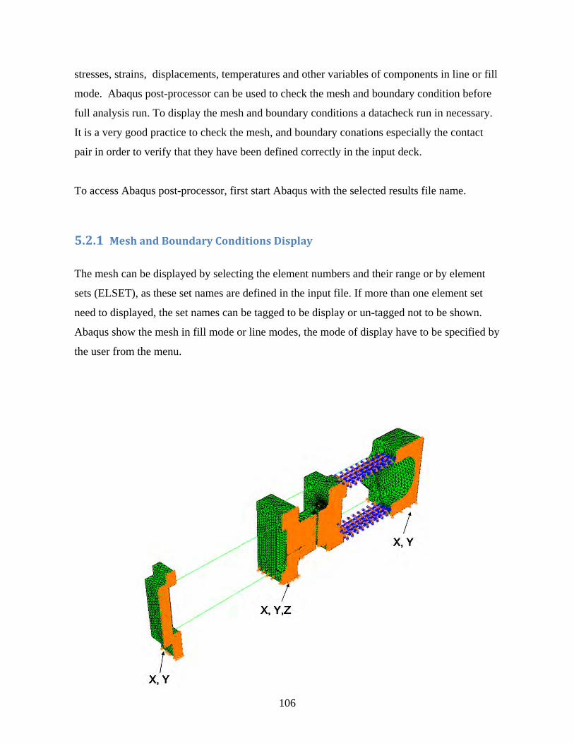
106
stresses, strains, displacements, temperatures and other variables of components in line or fill
mode. Abaqus post-processor can be used to check the mesh and boundary condition before
full analysis run. To display the mesh and boundary conditions a datacheck run in necessary.
It is a very good practice to check the mesh, and boundary conations especially the contact
pair in order to verify that they have been defined correctly in the input deck.
To access Abaqus post-processor, first start Abaqus with the selected results file name.
5.2.1MeshandBoundaryConditionsDisplay
The mesh can be displayed by selecting the element numbers and their range or by element
sets (ELSET), as these set names are defined in the input file. If more than one element set
need to displayed, the set names can be tagged to be display or un-tagged not to be shown.
Abaqus show the mesh in fill mode or line modes, the mode of display have to be specified by
the user from the menu.
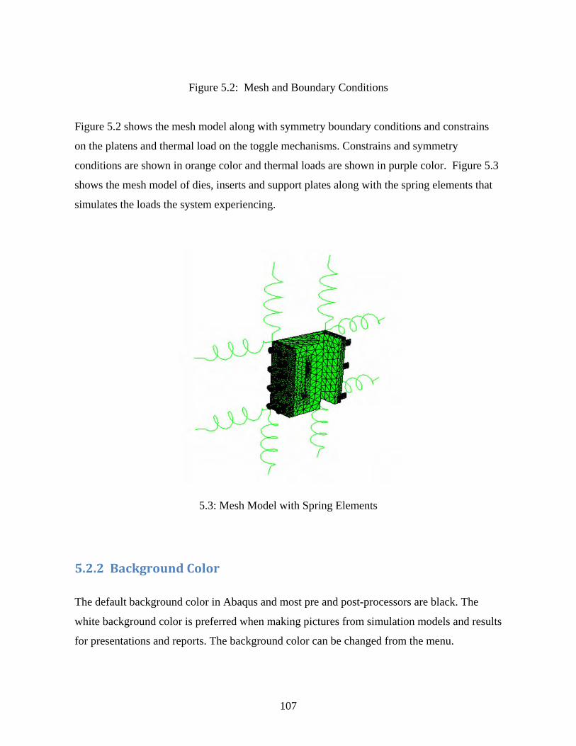
107
Figure 5.2: Mesh and Boundary Conditions
Figure 5.2 shows the mesh model along with symmetry boundary conditions and constrains
on the platens and thermal load on the toggle mechanisms. Constrains and symmetry
conditions are shown in orange color and thermal loads are shown in purple color. Figure 5.3
shows the mesh model of dies, inserts and support plates along with the spring elements that
simulates the loads the system experiencing.
5.3: Mesh Model with Spring Elements
5.2.2BackgroundColor
The default background color in Abaqus and most pre and post-processors are black. The
white background color is preferred when making pictures from simulation models and results
for presentations and reports. The background color can be changed from the menu.

108
5.2.3Viewing
The view buttons will change the viewing angle displayed objects. The fixed viewing angles
can show objects in isoperimetric, front, back, side view. Any other viewing angle can be
done by defining the unit vector of viewing angle in the menu. For example the unit vector of
(1, 1, 1) indicates an isoperimetric viewing vector. Also by selecting manual viewing the
curser can be moved in the viewing areas to change the viewing angle.
5.2.4DeformandUn‐deformShapesofComponents
The deform and un-deform shape of part or parts can be displayed by selecting the results file
and the element sets from the defined sets. The deform shape can be shown along with un-
deform shape in the line mode or fill mode. Also magnification factor can be selected, the
magnification factor is used to exaggerate the deform shape of parts relative to un-deform
shape. In most cases if magnification factors is one the deform and un-deform shape will
superimpose each other, while selecting a large magnification factor, for example 1000 or
2000, will result in a very unrealistic part display. The appropriate magnification factors can
be determined by selecting various magnification factors and plotting deform and un-deform
shapes.
Figure 5.4 displays the deform and un-deform shape of the casting part in fill mode. In this
plot the un-deformed shape in shown red color and deform shape in white in fill mode. In this
plot a magnification factor of 10 is used. This plot shows the deform and un-deform shapes
using elements in hidden form. In hidden form display shows only what can see seen from the
viewing angle, and will hide what is behind it.
In some cases it is better to display the deform and un-deform shapes by selecting outline
parameter as perimeter in the menu. In this way the plots will be more clear with less lines
and it can show subtle differences between deform and un-deform shapes of the parts. Also
these plots are better for presentation to be seen by observers which are not familiar in detail
with the parts.
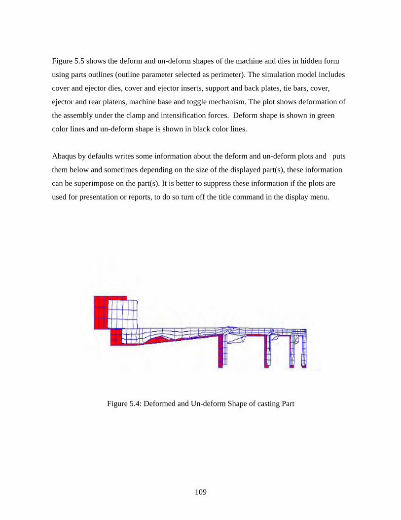
109
Figure 5.5 shows the deform and un-deform shapes of the machine and dies in hidden form
using parts outlines (outline parameter selected as perimeter). The simulation model includes
cover and ejector dies, cover and ejector inserts, support and back plates, tie bars, cover,
ejector and rear platens, machine base and toggle mechanism. The plot shows deformation of
the assembly under the clamp and intensification forces. Deform shape is shown in green
color lines and un-deform shape is shown in black color lines.
Abaqus by defaults writes some information about the deform and un-deform plots and puts
them below and sometimes depending on the size of the displayed part(s), these information
can be superimpose on the part(s). It is better to suppress these information if the plots are
used for presentation or reports, to do so turn off the title command in the display menu.
Figure 5.4: Deformed and Un-deform Shape of casting Part
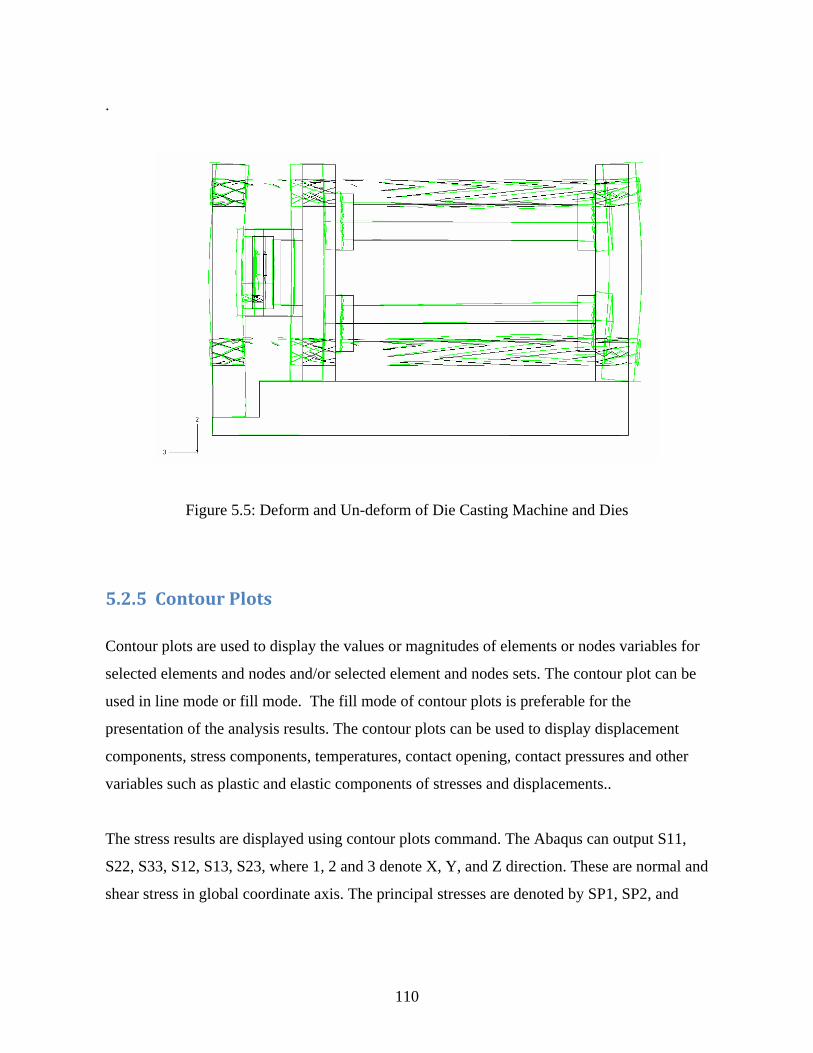
110
.
Figure 5.5: Deform and Un-deform of Die Casting Machine and Dies
5.2.5ContourPlots
Contour plots are used to display the values or magnitudes of elements or nodes variables for
selected elements and nodes and/or selected element and nodes sets. The contour plot can be
used in line mode or fill mode. The fill mode of contour plots is preferable for the
presentation of the analysis results. The contour plots can be used to display displacement
components, stress components, temperatures, contact opening, contact pressures and other
variables such as plastic and elastic components of stresses and displacements..
The stress results are displayed using contour plots command. The Abaqus can output S11,
S22, S33, S12, S13, S23, where 1, 2 and 3 denote X, Y, and Z direction. These are normal and
shear stress in global coordinate axis. The principal stresses are denoted by SP1, SP2, and
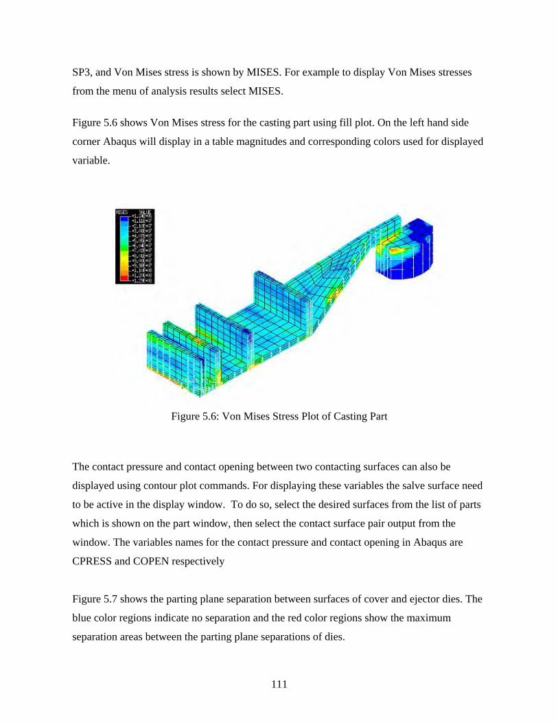
111
SP3, and Von Mises stress is shown by MISES. For example to display Von Mises stresses
from the menu of analysis results select MISES.
Figure 5.6 shows Von Mises stress for the casting part using fill plot. On the left hand side
corner Abaqus will display in a table magnitudes and corresponding colors used for displayed
variable.
Figure 5.6: Von Mises Stress Plot of Casting Part
The contact pressure and contact opening between two contacting surfaces can also be
displayed using contour plot commands. For displaying these variables the salve surface need
to be active in the display window. To do so, select the desired surfaces from the list of parts
which is shown on the part window, then select the contact surface pair output from the
window. The variables names for the contact pressure and contact opening in Abaqus are
CPRESS and COPEN respectively
Figure 5.7 shows the parting plane separation between surfaces of cover and ejector dies. The
blue color regions indicate no separation and the red color regions show the maximum
separation areas between the parting plane separations of dies.

112
Figure 5.8 show the contact pressure between the cover die and cover platen. The blue color
regions indicate low contact pressure areas and the red color regions indicate high contact
areas.
Figure 5.7: Parting Plane Separation between Dies

113
Figure 5.8: Contact Pressure between Cover Die and Cover Platen
5.2.6PartingPlaneSeparation
To display parting plane separation between the deformed dies and inserts surfaces relative to
initial contact planes requires the plot of the actual deformations of the cover side die and
insert contact surfaces and ejector side die and insert contact surfaces. When the clamp forces
are applied by toggle mechanism the tie bars will stretch, the tie bars stretches are elastic; this
deformation will displace the dies and inserts and will deform them too. A large portion
displaced dies and inserts are rigid body motion (rigid body displacement) and it will not
deform the dies and induce any stresses. The rigid motion part of displayed dies and inserts
should be removed from overall displacements of the both cover and ejector dies and inserts
contact surfaces. Once the intensification pressure and thermal loads are applied the
displacements of the dies and inserts surfaces will be adjusted according to these forces.
Plotting parting plane separation due to addition of intensification pressure and/or thermal
loads also requires removing the rigid body displacements of the dies and inserts due to the
clamp forces.
The die casting machine tie bars do not stretch uniformly (the tie bar forces are not equal), in
general, when the clamp force is applied. Each tie bar stretch (or its force) is also depends on

114
and adjusted by the intensification and thermal loads [13]. The die location on the platens will
distribute the clamp force on the tie bars. Tie bars force magnitudes are highly depends on the
die location on the platens. The final tie bar forces and resulting stretch when intensification
pressure and thermal loads are added is also by lesser degree depends on the location of the
cavity relative to the platen. The thermal loads will adjust the tie bars forces due to un-even
growth of the dies, this will happen when the temperature distribution on dies and inserts are
no symmetric.
Removing the rigid body displacements of the dies and inserts due to tie bar stretching
combined with any other forces will results in actual deform shapes relative to the initial
unloaded contact surface. Figure 5.5 displays the rigid body motion and displacement of the
dies and inserts. The black lines are the un-deformed shape and the green lines are the
deformed shape of the dies and die machine assembly.
The rigid body displacement can be removed from the predicted total displacements by using
a local coordinated system. The parting plane separations can be displayed by plotting
calculated displacements of the contact surfaces in this local coordinate system relative to
initial position of these surfaces. It is very important to mention that the nodes or points which
will be selected to construct this local coordinate system should the nodes or points that
remain in contact between and/or among the contacting surfaces (on the cover side die and
insert surfaces and on the ejector side die and insert surfaces) at all times and for all loads
steps. This condition will preserve the relative normal projection vector for all load cases and
the unit vector will not change with changing the forces or load cases. It is a very good
practice to check the direction of the constructed local coordinate system for al load steps and
cases and if needed to modify these nodes or points and select nodes or points that make them
( nodes and points) to remain in contact for all loads cases. The other import point is to select
nodes or points that are furthest from each other this will result in a local coordinate system
that will define unit vectors that relative calculated displacements are more sensitive to them.
If possible, the nodes can be selected near three corners of the dies.
The steps to plot parting plane are as follows

115
1- Plot two contact surfaces of the cover and ejector sides of the dies and inserts and
select the nodes or points that furthest from each other and remain in contact for all
loads cases by examining their deformation for all loads cases.
2- Construct a local coordinate system
3- Select the load case and plot deform and un-deform shapes in this local coordinate
system
Figure 5.9 shows the parting plane separation of the dies and inserts in line mode relative to
the nominal parting plane, initial contacting surface, for the cover and ejector dies and inserts.
The back lines show initial or nominal parting plane surfaces, the blue lines show the
displaced or distorted ejector side parting plane surface after removing the rigid body motion
of dies and the red lines show the displaced or distorted cover side parting plane surface after
the dies rigid body motion have been removed.
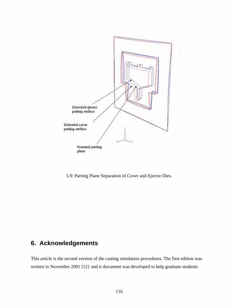
116
5.9: Parting Plane Separation of Cover and Ejector Dies.
6. Acknowledgements
This article is the second version of die casting simulation procedures. The first edition was
written in November 2001 [12} and it document was developed to help graduate students

117
doing research at the Center for Die Casting to get familiar with the modeling and analysis
procedures. This article was a web based documents.
The current article is the accumulation of the knowledge I have learned during my tenure at
the Center for Die Casting. During the past few years we, at the Center for Die Casting, have
refined and have developed new methods and procedures to simulate the die casting process.
Procedures have been developed to predict: tie bar forces, deflections and stresses in dies and
machine components, parting plane separation, casting part deformations, stresses and
residual stresses under mechanical and thermal loads. Some of these new procedures have
been compared with experimental data. The experiments which we, at the Center for Die
Casting, have designed them, conducted them, and collected data from them. The results of
comparisons in many cases are very satisfactory and very encouraging and they confirm the
validity of our simulation procedures.
The writing of this article and another article [13], for predicting tie bar forces and parting
plane separation using non-dimensional non-linear empirical correlations, were good
opportunities for me to document what I have learned by working with Dr. R. Allen Miller,
Head of the Center for Die Casting at The Ohio State University and the master and doctoral
students. Dr. Miller’s physical and fundamental knowledge of die casting processes is well
known and well respected and that is the way I learned them. I would like to give my greatest
thanks and appreciations to Dr. Miller who gave me many many opportunities to try my new
ideas, I also would like to thank all the graduate students that I worked, and they tried to
implements my new (may be old) ideas in their works. Some of these ideas worked, some did
not work, and some needed modification, and modifications were implemented which some
of these changes were proposed to me by Dr. Miller or by students. I would like to mention
the names of some of the graduate students whom I worked: Dr. Adham Ragab, Dr. Abelrado
Garza-Delgado, Dr. Karthik Murugesan, Eduardo Arrambide, Jeeth Kinatingal. Hongyu Xue,
and many others.
118
All the figures, plots and tables used in this manuscript were produced at the Center for Die
Casting by me and/or by students working at the center. I would like to thank all of them, the
persons I have mentioned and those I did not mention. Thank you all.
This article describes the most recent and common procedures that currently used at the
Center for Die Casting to simulate die casting process. A series of special procedures were
developed to simulate and predict casting part deformations, stresses and residual stresses and
die and also procedures were tested to simulate die casting machine behavior under dynamic
loads. These procedures are not explained here, The procedures and analysis details and
procedures can be found at [14,15,16,17,18,19,20,21,22].
7. References [1] Abaqus is a registered trade mark of Simulate www.simula.com [2] Magmasoft is a registered trade mark of Magma www.magmasoft.com [3] NX,/Ideas/Unigraphics are registered trade marks of Siemens PLM
www.plm.automation.siemens.com or www.unigraphics.com [4] Porcast is registered trade mark of ESI www.procast.com [5] Pro/E is registered trade mark of Tristar www.tristar.com [6] Catia is registered trade mark of Dassault System www.catia.com [7] AutoCad is registered trade mark of Autodesk www.autodesk.com [8] Ansys is registered trade mark of Ansys www.anays.com [9] Hypeworks/Hypermesh is registered trade mark of Altair www.altair.com [10] Patran is registered trade marc of MSC www.mscsoftware.com [11] Marc is registered trade marc of MSC www.mscsoftware.com [12] Kabiri, K., 2001, “Die Distortion Simulation,” Center for Die Casting, The Ohio State University.

119
[13] Kabiri-Bamoradian, K., 2009, “Die and Die Casting Machine Force and Deflection Predictions: Correlations for Predicting Tie Bar Forces and Parting Plane Separation,” Center for Die Casting, The Ohio State University. [14] Ragab, A., 2003, , "Sensitivity Analysis of Casting Distortion And residual Stress Prediction through Simulation Modeling And Experimental Verification," PhD Dissertation, The Ohio State University.
[15] Arrambide, E., 2004, "Modeling Influence of The Die Casting Machine Components on Contact Pressure between Dies and Platens," Master’s Thesis, The Ohio State University.
[16] Kinatingal, J.X., 2005, ‘Study of the effect of Structural and Machine Variables on Die deflection,” Master’s Dissertation, The Ohio State University.
[17] Xue, H., Kabiri-Bamoradian, K., and Miller, R. A., 2005, "Modeling the dynamic cavity pressure and impact spike in die casting," NADCA Transactions.
[18] Ragab, A., Kabiri-Bamoradian, K., and Miller, R. A., 2001, "Modeling part distortion and stresses in die casting," NADCA Transactions, pp. 77-83.
[19] Ragab, A., Kabiri-Bamoradian, K., and Miller, R. A., 2004, "Part distortion and stress prediction in die casting process: Sensitivity analysis," NADCA Transactions.
[20] Garza-Delgado, A., Kabiri-Bamoradian, K., and Miller, R. A., 2007, "Finite element modeling of casting distortion in die casting," NADCA transactions.
[21] Garza-Delgado, A, 2007, “A Study of Casting Distortion And Residual Stress in Die Casting , “PhD Dissertation, The Ohio State University.
[22] Murugesan, K. S., 2008, , "Predicting Parting Plane Separation And Tie Bar Loads in Die casting Using Computer Modeling and Dimensional Analysis," PhD Dissertation, The Ohio State University.