FIBER OPTICS -...

CHAPTER

8 FIBER OPTICS

8.1 STEP-INDEX FIBERS A. Guided Rays

B. Guided Waves C. Single-Mode Fibers

8.2 GRADED-INDEX FIBERS

A. Guided Waves B. Propagation Constants and Velocities

8.3 ATTENUATION AND DISPERSION A. Attenuation B. Dispersion

C. Pulse Propagation

Dramatic improvements in the development of low-loss materials for optical fibers are responsible for the commercial viability of fiber-optic communications. Corning Incorpo- rated pioneered the development and manufacture of ultra-low-loss glass fibers. C 0 R N I N G

272

Fundamentals of PhotonicsBahaa E. A. Saleh, Malvin Carl TeichCopyright © 1991 John Wiley & Sons, Inc.ISBNs: 0-471-83965-5 (Hardback); 0-471-2-1374-8 (Electronic)

An optical fiber is a cylindrical dielectric waveguide made of low-loss materials such as silica glass. It has a central core in which the light is guided, embedded in an outer cladding of slightly lower refractive index (Fig. 8.0-l). Light rays incident on the core-cladding boundary at angles greater than the critical angle undergo total internal reflection and are guided through the core without refraction. Rays of greater inclination to the fiber axis lose part of their power into the cladding at each reflection and are not guided.

As a result of recent technological advances in fabrication, light can be guided through 1 km of glass fiber with a loss as low as = 0.16 dB (= 3.6 %). Optical fibers are replacing copper coaxial cables as the preferred transmission medium for electromagnetic waves, thereby revolutionizing terrestrial communications. Applications range from long-distance telephone and data communications to computer communications in a local area network.

In this chapter we introduce the principles of light transmission in optical fibers. These principles are essentially the same as those that apply in planar dielectric waveguides (Chap. 71, except for the cylindrical geometry. In both types of waveguide light propagates in the form of modes. Each mode travels along the axis of the waveguide with a distinct propagation constant and group velocity, maintaining its transverse spatial distribution and its polarization. In planar waveguides, we found that each mode was the sum of the multiple reflections of a TEM wave bouncing within the slab in the direction of an optical ray at a certain bounce angle. This approach is approximately applicable to cylindrical waveguides as well. When the core diameter is small, only a single mode is permitted and the fiber is said to be a single-mode fiber. Fibers with large core diameters are multimode fibers.

One of the difficulties associated with light propagation in multimode fibers arises from the differences among the group velocities of the modes. This results in a variety of travel times so that light pulses are broadened as they travel through the fiber. This effect, called modal dispersion, limits the speed at which adjacent pulses can be sent without overlapping and therefore the speed at which a fiber-optic communication system can operate.

Modal dispersion can be reduced by grading the refractive index of the fiber core from a maximum value at its center to a minimum value at the core-cladding boundary. The fiber is then called a graded-index fiber, whereas conventional fibers

Figure 8.0-I An optical fiber is a cylindrical dielectric waveguide.

273

274 FIBER OPTICS

W --

(cl -- n1

I

n2 ---

a--

r

n1

me-_

-A-

-- n2

---

l}

nl ---

--

Figure 8.0-2 Geometry, refractive-index profile, and typical rays in: (a) a multimode step-index fiber, (b) a single-mode step-index fiber, and (c) a multimode graded-index fiber.

with constant refractive indices in the core and the cladding are called step-index fibers. In a graded-index fiber the velocity increases with distance from the core axis (since the refractive index decreases). Although rays of greater inclination to the fiber axis must travel farther, they travel faster, so that the travel times of the different rays are equalized. Optical fibers are therefore classified as step-index or graded-index, and multimode or single-mode, as illustrated in Fig. 8.0-2.

This chapter emphasizes the nature of optical modes and their group velocities in step-index and graded-index fibers. These topics are presented in Sets. 8.1 and 8.2, respectively. The optical properties of the fiber material (which is usually fused silica), including its attenuation and the effects of material, modal, and waveguide dispersion on the transmission of light pulses, are discussed in Sec. 8.3. Optical fibers are revisited in Chap. 22, which is devoted to their use in lightwave communication systems.

8.1 STEP-INDEX FIBERS

A step-index fiber is a cylindrical dielectric waveguide specified by its core and cladding refractive indices, ~zr and n2, and the radii a and b (see Fig. 8.0-l). Examples of standard core and cladding diameters 2a/2b are S/125, 50/125, 62.5/125, 85/125, 100/140 (units of pm). The refractive indices differ only slightly, so that the fractional refractive-index change

A = ‘l - n2 (8.1-1) nl

is small (A < 1). Almost all fibers currently used in optical communication systems are made of fused

silica glass (SiO,) of high chemical purity. Slight changes in the refractive index are

STEP-INDEX FIBERS 275

made by the addition of low concentrations of doping materials (titanium, germanium, or boron, for example). The refractive index y1r is in the range from 1.44 to 1.46, depending on the wavelength, and A typically lies between 0.001 and 0.02.

A. Guided Rays

An optical ray is guided by total internal reflections within the fiber core if its angle of incidence on the core-cladding boundary is greater than the critical angle 8, = sin - ‘(n,/nt ), and remains so as the ray bounces.

Meridional Rays The guiding condition is simple to see for meridional rays (rays in planes passing through the fiber axis), as illustrated in Fig. 8.1-l. These rays intersect the fiber axis and reflect in the same plane without changing their angle of incidence, as if they were in a planar waveguide. Meridional rays are guided if their angle 8 with the fiber axis is smaller than the complement of the critical angle GC = VT/~ - 8, = cos-l&/n,). Since rrr = n2, 8, is usually small and the guided rays are approximately paraxial.

Meridional plane

Figure 8.1-1 The trajectory of a meridional ray lies in a plane passing through the fiber axis. The ray is guided if 8 < aC = cos-‘(n,/n,).

Skewed Rays An arbitrary ray is identified by its plane of incidence, a plane parallel to the fiber axis and passing through the ray, and by the angle with that axis, as illustrated in Fig. 8.1-2. The plane of incidence intersects the core-cladding cylindrical boundary at an angle C#I with the normal to the boundary and lies at a distance R from the fiber axis. The ray is identified by its angle 8 with the fiber axis and by the angle 4 of its plane. When 4 # 0 (R f 0) the ray is said to be skewed. For meridional rays C$ = 0 and R = 0.

A skewed ray reflects repeatedly into planes that make the same angle 4 with the core-cladding boundary, and follows a helical trajectory confined within a cylindrical shell of radii R and a, as illustrated in Fig. 8.1-2. The projection of the trajectory onto the transverse (x-y) plane is a regular polygon, not necessarily closed. It can be shown that the condition for a skewed ray to always undergo total internal reflection is that its angle 0 with the z axis be smaller than aC.

Numerical Aperture A ray incident from air into the fiber becomes a guided ray if upon refraction into the core it makes an angle 8 with the fiber axis smaller than gC. Applying Snell’s law at the air-core boundary, the angle 8, in air corresponding to gC in the core is given by the relation 1 - sin 0, = nr sin gC, from which (see Fig. 8.1-3 and Exercise 1.2-5) sin e a = n (1 I - cos2e )li2 c = n,[l - (n2/n1)2]‘/2 = (ny - n;)‘/2. Therefore

8, = sin-’ NA, (8.1-2)

276 FIBER OPTICS

a x

Figure 8.1-2 A skewed ray lies in a plane offset from the fiber axis by a distance R. The ray is identified by the angles 8 and 4. It follows a helical trajectory confined within a cylindrical shell of radii R and a. The projection of the ray on the transverse plane is a regular polygon that is not necessarily closed.

where

1 NA = (4 - w2 = n1wY2 1 ,,,,,ica,~;;‘,;“,;

is the numerical aperture of the fiber. Thus 8, is the acceptance angle of the fiber. It

Unguided Guided

Small NA

Large NA

Figure 8.1-3 (a) The acceptance angle 8, of a fiber. Rays within the acceptance cone are guided by total internal reflection. The numerical aperture NA = sin 8,. (b) The light-gathering capacity of a large NA fiber is greater than that of a small NA fiber. The angles 8, and gC are typically quite small; they are exaggerated here for clarity.


determines the cone of external rays that are guided by the fiber. Rays incident at angles greater than 8, are refracted into the fiber but are guided only for a short distance. The numerical aperture therefore describes the light-gathering capacity of the fiber.

When the guided rays arrive at the other end of the fiber, they are refracted into a cone of angle 8,. Thus the acceptance angle is a crucial parameter for the design of systems for coupling light into or out of the fiber.

EXAMPLE 8.1-l. C/added and Uncladded Fibers. In a silica glass fiber with izl = 1.46 and A = (n, - n2)/n1 = 0.01, the complementary critical angle gC = cos-‘(n/n,) = 8.1”, and the acceptance angle 8, = 11.9”, corresponding to a numerical aperture NA = 0.206. By comparison, an uncladded silica glass fiber (n, = 1.46, n2 = 1) has e, = 46.8”, Ba = 90”, and NA = 1. Rays incident from all directions are guided by the uncladded fiber since they reflect within a cone of angle SC = 46.8” inside the core. Although its light-gathering capacity is high, the uncladded fiber is not a suitable optical waveguide because of the large number of modes it supports, as will be shown subsequently.

B. Guided Waves

In this section we examine the propagation of monochromatic light in step-index fibers using electromagnetic theory. We aim at determining the electric and magnetic fields of guided waves that satisfy Maxwell’s equations and the boundary conditions imposed by the cylindrical dielectric core and cladding. As in all waveguides, there are certain special solutions, called modes (see Appendix C), each of which has a distinct propagation constant, a characteristic field distribution in the transverse plane, and two independent polarization states.

Spatial Distributions Each of the components of the electric and magnetic fields must satisfy the Helmholtz equation, V2U + n2kzU = 0, where n = ~1~ in the core (r < a) and n = n2 in the cladding (r > a) and k, = 27r/A, (see Sec. 5.3). We assume that the radius b of the cladding is sufficiently large that it can safely be assumed to be infinite when examining guided light in the core and near the core-cladding boundary. In a cylindrical coordinate system (see Fig. 8.1-4) the Helmholtz equation is

a2u 1 au 1 a2u a2u p+;~+~~+~+n2k~U=0,

r a4 (8.1-4)

Cladding

Figure 8.1-4 Cylindrical coordinate system.

278 FIBER OPTICS

where the complex amplitude U = U(r, 4, z) represents any of the Cartesian components of the electric or magnetic fields or the axial components E, and Hz in cylindrical coordinates.

We are interested in solutions that take the form of waves traveling in the z direction with a propagation constant /3, so that the z dependence of U is of the form e . -j@ Since U must be a periodic function of the angle 4 with period 2~, we assume that the dependence on 4 is harmonic, e-j@‘, where I is an integer. Substituting

U( r, 4, z) = u( r)e-ir4e-jpz, I = 0, * 1, * 2,. . . , (8.1-5)

into (8.1-4), an ordinary differential equation for U(T) is obtained:

d2u 1 du z+;~+ (8.1-6)

As in Sec. 7.2B, the wave is guided (or bound) if the propagation constant is smaller than the wavenumber in the core (p < n,k,) and greater than the wavenumber in the cladding (/3 > n,k,). It is therefore convenient to define

and

kf = n:kz - p2 (8.1-7a)

y2 = p2 - nzkz, (8.1-7b)

so that for guided waves k; and y2 are positive and k, and y are real. Equation (8.1-6) may then be written in the core and cladding separately:

r < a (core), (8.1-8a)

r > a (cladding). (8.1-8b)

Equations (8.1-8) are well-known differential equations whose solutions are the family of Bessel functions. Excluding functions that approach 03 at r = 0 in the core or at r + a in the cladding, we obtain the bounded solutions:

u(r) a J&r) 7 r < a (core)

KkYr) 7 r > a (cladding), (8.1-9)

where J[(x) is the Bessel function of the first kind and order 1, and K,(x) is the modified Bessel function of the second kind and order 1. The function J,(x) oscillates like the sine or cosine functions but with a decaying amplitude. In the limit x z+ 1,

J,(X) = (h)l/lw~[~ - (I + +);I, x x=- 1. (8.1-10a)

u(r) t


44

t

*~ o

0 a r

(a) lb)

Figure 8.1-5 Examples of the radial distribution U(T) given by (8.1-9) for (a) 1 = 0 and (b) 1 = 3. The shaded areas represent the fiber core and the unshaded areas the cladding. The parameters k, and y and the two proportionality constants in (8.1-9) have been selected such that u(r) is continuous and has a continuous derivative at r = a. Larger values of k, and y lead to a greater number of oscillations in U(T).

In the same limit, K,(x) decays with increasing x at an exponential rate,

412 - 1 1 + 8x ew( -x>, x x=- 1. (8.1-lob)

Two examples of the radial distribution U(T) are shown in Fig. 8.1-S. The parameters k, and y determine the rate of change of U(T) in the core and in

the cladding, respectively. A large value of k, means faster oscillation of the radial distribution in the core. A large value of y means faster decay and smaller penetration of the wave into the cladding. As can be seen from (8.1-7), the sum of the squares of k, and y is a constant,

k; + y2 = (nf - n;)k; = NA2 + k;, (8.1-11)

so that as k, increases, y decreases and the field penetrates deeper into the cladding. As k, exceeds NA- k,, y becomes imaginary and the wave ceases to be bound to the core.

The V Parameter It is convenient to normalize k, and y by defining

X = kTa, Y= ya. (8.1-12)

In view of (&l-11),

x2 + Y2 = v2, (8.1-13)

where V = NA * k,a, from which

1 V = 2rFNA. (8.1-14) 0 V Parameter

As we shall see shortly, V is an important parameter that governs the number of modes

280 FIBER OPTICS

of the fiber and their propagation constants. It is called the fiber parameter or V parameter. It is important to remember that for the wave to be guided, X must be smaller than V.

Modes We now consider the boundary conditions. We begin by writing the axial components of the electric- and magnetic-field complex amplitudes E, and Hz in the form of (8.1-5). The condition that these components must be continuous at the core-cladding boundary r = a establishes a relation between the coefficients of proportionality in (8.1-9), so that we have only one unknown for E, and one unknown for Hz. With the help of Maxwell’s equations, jwe0n2E = V x H and -jopOH = V X E, the remaining four components E,, H4, E,., and Hr are determined in terms of E, and Hz. Continuity of E, and H4 at r = a yields two more equations. One equation relates the two unknown coefficients of proportionality in E, and Hz; the other equation gives a condition that the propagation constant p must satisfy. This condition, called the characteristic equation or dispersion relation, is an equation for p with the ratio a/h, and the fiber indices n 1, n2 as known parameters.

For each azimuthal index I, the characteristic equation has multiple solutions yielding discrete propagation constants plm, m = 1,2,. . . , each solution representing a mode. The corresponding values of k, and y, which govern the spatial distributions in the core and in the cladding, respectively, are determined by use of (8.1-7) and are denoted kTlm and ylm. A mode is therefore described by the indices 1 and m characterizing its azimuthal and radial distributions, respectively. The function U(T) depends on both I and m; 2 = 0 corresponds to meridional rays. There are two independent configurations of the E and H vectors for each mode, corresponding to two states of polarization. The classification and labeling of these configurations are generally quite involved (see specialized books in the reading list for more details).

Characteristic Equation for the Weakly Guiding Fiber Most fibers are weakly guiding (i.e., y1r = n2 or A < 1) so that the guided rays are paraxial (i.e., approximately parallel to the fiber axis). The longitudinal components of the electric and magnetic fields are then much weaker than the transverse components and the guided waves are approximately transverse electromagnetic (TEM). The linear polarization in the x and y directions then form orthogonal states of polarization. The linearly polarized (I, m) mode is usually denoted as the LP,, mode. The two polarizations of mode (I, m) travel with the same propagation constant and have the same spatial distribution.

For weakly guiding fibers the characteristic equation obtained using the procedure outlined earlier turns out to be approximately equivalent to the conditions that the scalar function U(T) in (8.1-9) is continuous and has a continuous derivative at r = a. These two conditions are satisfied if

The derivatives Ji and Ki of the Bessel functions satisfy the identities

(8.1-15)

J,(x) J/(x) = +Jlqzl(~) + I-

X

K,(x) K/(x) = -K/.,(X) T l-

x *


Substituting these identities into (8.1-15) and using the normalized parameters X = k,a and Y = ya, we obtain the characteristic equation

(8.1-16) Characteristic

Equation

X2+Y2=V2

Given V and I, the characteristic equation contains a single unknown variable X (since Y2 = V2 - X2). Note that J-&x) = (- l)‘J[(x) and K-,(x) = K,(x), so that if I is replaced with -I, the equation remains unchanged.

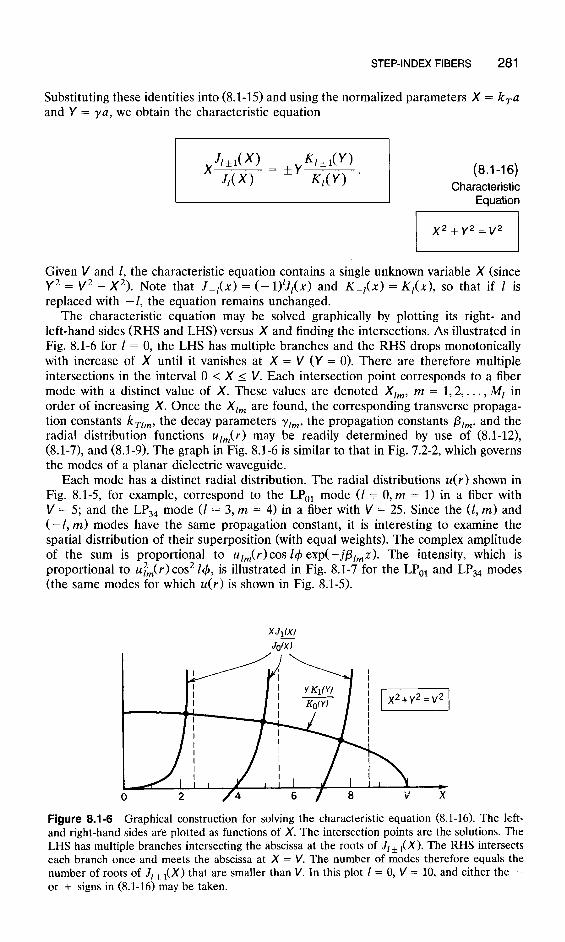
The characteristic equation may be solved graphically by plotting its right- and left-hand sides (RHS and LHS) versus X and finding the intersections. As illustrated in Fig. 8.1-6 for I = 0, the LHS has multiple branches and the RHS drops monotonically with increase of X until it vanishes at X = V (V = 0). There are therefore multiple intersections in the interval 0 < X i V. Each intersection point corresponds to a fiber mode with a distinct value of X. These values are denoted Xlm, m = 1,2,. . . , M[ in order of increasing X. Once the X,, are found, the corresponding transverse propagation constants kTlm, the decay parameters yfm, the propagation constants firm, and the radial distribution functions ulm(r) may be readily determined by use of (&l-12), (8.1-7), and (8.1-9). The graph in Fig. 8.1-6 is similar to that in Fig. 7.2-2, which governs the modes of a planar dielectric waveguide.

Each mode has a distinct radial distribution. The radial distributions U(T) shown in Fig. 8.1-5, for example, correspond to the LP,, mode (I = 0, m = 1) in a fiber with V = 5; and the LP,, mode (I = 3, m = 4) in a fiber with V = 25. Since the (1, m) and (-I, m) modes have the same propagation constant, it is interesting to examine the spatial distribution of their superposition (with equal weights). The complex amplitude of the sum is proportional to U/~(T) cos Z4 exp( -jplmz). The intensity, which is proportional to u;~(I-) cos2 Z& is illustrated in Fig. 8.1-7 for the LP,, and LP,, modes (the same modes for which U(T) is shown in Fig. 8.1-S).

X JlCX,

JO(X)

O

Figure 8.1-6 Graphical construction for solving the characteristic equation (8.1-16). The left- and right-hand sides are plotted as functions of X. The intersection points are the solutions. The LHS has multiple branches intersecting the abscissa at the roots of JI f r(X). The RHS intersects each branch once and meets the abscissa at X = V. The number of modes therefore equals the number of roots of JI + r(X) that are smaller than V. In this plot 1 = 0, V = 10, and either the - or + signs in (8.1-16) may be taken.

282 FIBER OPTICS

Figure 8.1-7 Distributions of the intensity of the (a) LP,, and (b) LP34 modes in the transverse plane, assuming an azimuthal cos 14 dependence. The fundamental LPO, mode has a distribution similar to that of the Gaussian beam discussed in Chap. 3. fb)

Mode Cutoff and Number of Modes It is evident from the graphical construction in Fig. 8.1-6 that as V increases, the number of intersections (modes) increases since the LHS of the characteristic equation (8.1-16) is independent of I/, whereas the RHS moves to the right as V increases. Considering the minus signs in the characteristic equation, branches of the LHS intersect the abscissa when J,-,(X) = 0. These roots are denoted by xlm, m = 1,2,. . . . The number of modes Ml is therefore equal to the number of roots of JI- ,(X) that are smaller than V. The (I, m) mode is allowed if V > xlm. The mode reaches its cutoff point when V = xlm. As V decreases further, the (I, m - 1) mode also reaches its cutoff point when a new root is reached, and so on. The smallest root of JIpl(X) is xol = 0 for I = 0 and the next smallest is xI1 = 2.405 for 1 = 1. When V < 2.405, all modes with the exception of the fundamental LPol mode are cut off. The fiber then operates as a single-mode waveguide. A plot of the number of modes Mr as a function of V is therefore a staircase function increasing by unity at each of the roots xl,,, of the Bessel function J,-,(X). Some of these roots are listed in Table 8.1-1.

TABLE 8.1-1 Cutoff V Parameter for the LP,, and LP,, Mode#

1 m: 1 2 3

0 0 3.832 7.016 1 2.405 5.520 8.654

‘The cutoffs of the I = 0 modes occur at the roots of L,(X) = -J,(X). The 1 = 1 modes are cut off at the roots of J,(X), and so on.


50

40 . ‘r, z “0 30 E

6

ij 20 E 3

= 10

0 0 2 4 6 8

V

Figure 8.1-8 Total number of modes M versus the fiber parameter V = 2r(a/A,JNA. In- cluded in the count are two helical polarities for each mode with I > 0 and two polarizations per mode. For V < 2.405, there is only one mode, the fundamental LP,,, mode with two polarizations. The dashed curve is the relation M = 4V2/7r2 + 2, which provides an approximate formula for the number of modes when V x=- 1.

A composite count of the total number of modes M (for all I) is shown in Fig. 8.1-8 as a function of V. This is a staircase function with jumps at the roots of JImI( Each root must be counted twice since for each mode of azimuthal index I > 0 there is a corresponding mode -1 that is identical except for an opposite polarity of the angle C$ (corresponding to rays with helical trajectories of opposite senses) as can be seen by using the plus signs in the characteristic equation. In addition, each mode has two states of polarization and must therefore be counted twice.

Number of Modes (Fibers with Large V Parameter) For fibers with large V parameters, there are a large number of roots of J,(X) in the interval 0 < X < V. Since J,(X) is approximated by the sinusoidal function in (8.1-10a) when X B 1, its roots xlm are approximately given by xl,,, - (I + iX7r/2) = (2m - 1)(7~/2), i.e., xlm = (I + 2m - $)~/2, so that the cutoff points of modes (I, m), which are th e roots of J, + ,(X), are -

xlm = i /+2+1 f

1 = (l+ 24, I = O,l,...; m Z- 1, (8.1-17)

when m is large. For a fixed I, these roots are spaced uniformly at a distance r, so that the number

of roots Ml satisfies (1 + 2M,)7r/2 = V, from which M, = V/T - Z/2. Thus h4/ drops linearly with increasing I, beginning with M, = V/T for 1 = 0 and ending at i’MI = 0 when I = Imax, where I,, = 2V/7r, as illustrated in Fig. 8.1-9. Thus the total number of modes is M = L&m, = Q‘$V/a - l/2).

Since the number of terms in this sum is assumed large, it may be readily evaluated by approximating it as the area of the triangle in Fig. 8.1-9, M = +(~V/TXV/T) = V2/r2. Allowing for two degrees of freedom for positive and negative I and two polarizations for each index (I, m), we obtain

(8.148) Number of Modes

(Vx=+ 1)

284 FIBER OPTICS

Figure 8.1-9 The indices of guided modes extend from m = 1 to m = V/r - l/2 and from 1 = 0 to 2: ~V/T.

0 0 v/n m

This expression for A4 is analogous to that for the rectangular waveguide (7.3-3). Note that (8.1-18) is valid only for large V. This approximate number is compared to the exact number obtained from the characteristic equation in Fig. 8.1-8.

EXAMPLE 8.1-2. Approximate Number of Modes. A silica fiber with nl = 1.452 and A = 0.01 has a numerical aperture NA = (n: - nz)1/2 = n1(2Aj1i2 = 0.205. If A, = 0.85 pm and the core radius a = 25 pm, the V parameter is V = 2r(a/A,)NA = 37.9. There are therefore approximately M = 4V2/7r2 = 585 modes. If the cladding is stripped away so that the core is in direct contact with air, n2 = 1 and NA = 1. The V parameter is then V = 184.8 and more than 13,800 modes are allowed.

Propagation Constants (Fibers with Large V Parameter) As mentioned earlier, the propagation constants can be determined by solving the characteristic equation (8.1-16) for the X,, and using (8.1-7a) and (8.1-12) to obtain PI,,, = (nfkz - X&/a2)1/2. A number of approximate formulas for X,, applicable in certain limits are available in the literature, but there are no explicit exact formulas.

If V z+ 1, the crudest approximation is to assume that the X,, are equal to the cutoff values xlm. This is equivalent to assuming that the branches in Fig. 8.1-6 are approximately vertical lines, so that Xrm = xlm. Since V z=- 1, the majority of the roots would be large and the approximation in (8.1-17) may be used to obtain

7r2 1 l/2

P lm = nfk,2 - (1 + 2rr1)‘~ . (8.1-19)

Since

M= -$V2 = 5NA2. a2kz = -$(lnfl)k:o”, (8.1-20)

(8.1-19) and (8.1-20) give

(8.1-21)

Because A is small we use the approximation (1 + 8)li2 = 1 + 6/2 for 161 GE 1, and


n2kJ

n1k0

---------- / n2kJ

0 / d= /

. . . . . . . . . . . . ml

. . . .

v% A- 2 m

n&J

PO1

012345 2

(61

Figure 8.1-10 (a) Approximate propagation constants Plm of the modes of a fiber with large V parameter as functions of the mode indices 1 and m. (b) Exact propagation constant PO1 of the fundamental LPO, modes as a function of the V parameter. For V B 1, PO1 = nlk,.

obtain

Since 1 + 2m varies between 2 and = 2V/7~ = m (see Fig. 8.1-9), PI,,, varies approximately between nlko and n,k,(l - A) = nzko, as illustrated in Fig. 8.1-10.

Group Velocities (Fibers with Large V Parameter) To determine the group velocity, vim = do/dp,,, of the (I, m) mode we express Plrn as an explicit function of o by substituting nlko = o/c1 and A4 = (4/r2)(2nfA)k$z2 = (8/r2)a2ti2A/cf into (8.1-22) and assume that cr and A are independent of o. The derivative do/d/?,, gives

(1 -I- 2mj2 -l vim A .

A4 1 Since A -=K 1, the approximate expansion (1 + S)-’ = 1 - 6 when ISI -=z 1, gives

Because the minimum and maximum values of (1 + 2m) are 2 and m, respectively, and since A4 x=- 1, the group velocity varies approximately between c r and c,(l - A) = c1(n2/nz1). Thus the group velocities of the low-order modes are approximately equal to the phase velocity of the core material, and those of the high-order modes are smaller.

286 FIBER OPTICS

The fractional group-velocity change between the fastest and the slowest mode is roughly equal to A, the fractional refractive index change of the fiber. Fibers with large A, although endowed with a large NA and therefore large light-gathering capacity, also have a large number of modes, large modal dispersion, and consequently high pulse spreading rates. These effects are particularly severe if the cladding is removed altogether.

C. Single-Mode Fibers

As discussed earlier, a fiber with core radius a and numerical aperture NA operates as a single-mode fiber in the fundamental LP,, mode if V = 2r(a/A,)NA < 2.405 (see Table 8.1-1 on page 282). Single-mode operation is therefore achieved by using a small core diameter and small numerical aperture (making n2 close to ni), or by operating at a sufficiently long wavelength. The fundamental mode has a bell-shaped spatial distribution similar to the Gaussian distribution [see Figs. 8.1-5(a) and 8.1-7(a)] and a propagation constant /3 that depends on V as illustrated in Fig. 8.1-10(b). This mode provides the highest confinement of light power within the core.

EXAMPLE 8.1-3. Single-Mode Operation. A silica glass fiber with n1 = 1.447 and A = 0.01 (NA = 0.205) operates at A, = 1.3 pm as a single-mode fiber if V = 2r(a/A,)NA < 2.405, i.e., if the core diameter 2a < 4.86 pm. If A is reduced to 0.0025, single-mode operation requires a diameter 2a < 9.72 pm.

There are numerous advantages of using single-mode fibers in optical communication systems. As explained earlier, the modes of a multimode fiber travel at different group velocities and therefore undergo different time delays, so that a short-duration pulse of multimode light is delayed by different amounts and therefore spreads in time. Quantitative measures of modal dispersion are determined in Sec. 8.3B. In a single- mode fiber, on the other hand, there is only one mode with one group velocity, so that a short pulse of light arrives without delay distortion. As explained in Sec. 8.3B, other dispersion effects result in pulse spreading in single-mode fibers, but these are significantly smaller than modal dispersion.

As also shown in Sec. 8.3, the rate of power attenuation is lower in a single-mode fiber than in a multimode fiber. This, together with the smaller pulse spreading rate, permits substantially higher data rates to be transmitted by single-mode fibers in comparison with the maximum rates feasible with multimode fibers. This topic is discussed in Chap. 22.

Another difficulty with multimode fibers is caused by the random interference of the modes. As a result of uncontrollable imperfections, strains, and temperature fluctuations, each mode undergoes a random phase shift so that the sum of the complex amplitudes of the modes has a random intensity. This randomness is a form of noise known as modal noise or speckle. This effect is similar to the fading of radio signals due to multiple-path transmission. In a single-mode fiber there is only one path and therefore no modal noise.

Because of their small size and small numerical apertures, single-mode fibers are more compatible with integrated-optics technology. However, such features make them more difficult to manufacture and work with because of the reduced allowable mechanical tolerances for splicing or joining with demountable connectors and for coupling optical power into the fiber.

GRADED-INDEX FIBERS 287

Polarization 1

ia)

_I=L_, I , Polarization 1 .I& 0

Polarization 2 Polarization 2

Polarization 1 .I

ib)

Polarization 2 Polarization 2 33l + t t

Figure 8.1-l 1 (a) two polarizations.

Ideal polarization-maintaining fiber. (b) Random transfer of power between

Polarization-Maintaining Fibers In a fiber with circular cross section, each mode has two independent states of polarization with the same propagation constant. Thus the fundamental LPO, mode in a single-mode weakly guiding fiber may be polarized in the x or y direction with the two orthogonal polarizations having the same propagation constant and the same group velocity.

In principle, there is no exchange of power between the two polarization components. If the power of the light source is delivered into one polarization only, the power received remains in that polarization. In practice, however, slight random imperfections or uncontrollable strains in the fiber result in random power transfer between the two polarizations. This coupling is facilitated since the two polarizations have the same propagation constant and their phases are therefore matched. Thus linearly polarized light at the fiber input is transformed into elliptically polarized light at the output. As a result of fluctuations of strain, temperature, or source wavelength, the ellipticity of the received light fluctuates randomly with time. Nevertheless, the total power remains fixed (Fig. 8.1-11). If we are interested only in transmitting light power, this randomiza- tion of the power division between the two polarization components poses no difficulty, provided that the total power is collected.

In many areas related to fiber optics, e.g., coherent optical communications, integrated-optic devices, and optical sensors based on interferometric techniques, the fiber is used to transmit the complex amplitude of a specific polarization (magnitude and phase). For these applications, polarization-maintaining fibers are necessary. To make a polarization-maintaining fiber the circular symmetry of the conventional fiber must be removed, by using fibers with elliptical cross sections or stress-induced anisotropy of the refractive index, for example. This eliminates the polarization degeneracy, i.e., makes the propagation constants of the two polarizations different. The coupling efficiency is then reduced as a result of the introduction of phase mismatch.

8.2 GRADED-INDEX FIBERS

Index grading is an ingenious method for reducing the pulse spreading caused by the differences in the group velocities of the modes of a multimode fiber. The core of a graded-index fiber has a varying refractive index, highest in the center and decreasing gradually to its lowest value at the cladding. The phase velocity of light is therefore minimum at the center and increases gradually with the radial distance. Rays of the

288 FIBER OPTICS

n2 n1 n

Figure 8.2-l Geometry and refractive-index profile of a graded-index fiber.

most axial mode travel the shortest distance at the smallest phase velocity. Rays of the most oblique mode zigzag at a greater angle and travel a longer distance, mostly in a medium where the phase velocity is high. Thus the disparities in distances are compensated by opposite disparities in phase velocities. As a consequence, the differences in the group velocities and the travel times are expected to be reduced. In this section we examine the propagation of light in graded-index fibers.

The core refractive index is a function n(r) of the radial position r and the cladding refractive index is a constant n2. The highest value of n(r) is n(O) = n1 and the lowest value occurs at the core radius r = a, n(a) = n2, as illustrated in Fig. 8.2-l.

A versatile refractive-index profile is the power-law function

n2(r) =nf[l - 2(k)'A], r 5 a, (8.2-l)

where

A= n: - nz nl - n2

xy= ,

n1

(8.2-2)

and p, called the grade profile parameter, determines the steepness of the profile. This function drops from n1 at r = 0 to n2 at r = a. For p = 1, n2(r) is linear, and for p = 2 it is quadratic. As p + 03, n2(r) approaches a step function, as illustrated in Fig. 8.2-2. Thus the step-index fiber is a special case of the graded-index fiber with p = 00.

Guided Rays The transmission of light rays in a graded-index medium with parabolic-index profile was discussed in Sec. 1.3. Rays in meridional planes follow oscillatory planar trajecto-

P = 1

n$ nf e

n2

Figure 8.2-2 Power-law refractive-index profile n2(r) for different values of p.


fb)

Figure 8.2-3 Guided rays in the core of a graded-index fiber. (a) A meridional ray confined to a meridional plane inside a cylinder of radius R,. (b) A skewed ray follows a helical trajectory confined within two cylindrical shells of radii rf and R,.

ries, whereas skewed rays follow helical trajectories with the turning points forming cylindrical caustic surfaces, as illustrated in Fig. 8.2-3. Guided rays are confined within the core and do not reach the cladding.

A. Guided Waves

The modes of the graded-index fiber may be determined by writing the Helmholtz equation (8.1-4) with n = n(r), solving for the spatial distributions of the field components, and using Maxwell’s equations and the boundary conditions to obtain the characteristic equation as was done in the step-index case. This procedure is in general difficult.

In this section we use instead an approximate approach based on picturing the field distribution as a quasi-plane wave traveling within the core, approximately along the trajectory of the optical ray. A quasi-plane wave is a wave that is locally identical to a plane wave, but changes its direction and amplitude slowly as it travels. This approach permits us to maintain the simplicity of rays optics but retain the phase associated with the wave, so that we can use the self-consistency condition to determine the propagation constants of the guided modes (as was done in the planar waveguide in Sec. 7.2). This approximate technique, called the WKB (Wentzel-Kramers-Brillouin) method, is applicable only to fibers with a large number of modes (large V parameter).

Quasi-Plane Waves Consider a solution of the Helmholtz equation (8.1-4) in the form of a quasi-plane wave (see Sec. 2.3)

W = 49 ew[ -jk,S(d] , (8.2-3)

where a(r) and S(r) are real functions of position that are slowly varying in comparison with the wavelength h, = 2r/k,. We know from Sec. 2.3 that S(r) approximately

290 FIBER OPTICS

satisfies the eikonal equation (VS12 = n2, and that the rays travel in the direction of the gradient VS. If we take k,S(r) = k,~(r) + Z4 + pz, where S(Y) is a slowly varying function of r, the eikonal equation gives

2 l2 + p2 + 7 = n2(r)kz. (8.2-4)

The local spatial frequency of the wave in the radial direction is the partial derivative of the phase k,S(r) with respect to r,

kr=ko;,

so that (8.2-3) becomes

(8.2-5)

and (8.2-4) gives

1 l2

k; = n2(r)kz - p2 - 7. (8.2-7)

I

Defining k, = l/r, i.e., exp(-jZ+) = exp( -jk,r+), and k, = p, we find that (8.2-7) gives kz + k$ + kz = n2(r)k$ The quasi-plane wave therefore has a local wavevector k with magnitude n(r)k, and cylindrical-coordinate components (k,, k,, k,). Since n(r) and k, are functions of r, k, is also generally position dependent. The direction of k changes slowly with r (see Fig. 8.2-4) following a helical trajectory similar to that of the skewed ray shown earlier in Fig. 8.2-3(b).

Figure 8.2-4 (a) The wavevector k = (k,, k,, k,) in a cylindrical coordinate system. (b) Quasi-plane wave following the direction of a ray.


a .2k2 - 12

0

/

r2

n2k2 lo n2k2

lo

(a) (b)

Figure 8.2-5 Dependence of n2(r)kz, n2(r)kz - 12/r2, and k: = n2(r)kz - Z2/r2 - p2 on the position r. At any r, kf is the width of the shaded area with the + and - signs denoting positive and negative k;. (a) Graded-index fiber; k; is positive in the region rl < r < R,. (b) Step-index fiber; kf is positive in the region rl < r < a.

To determine the region of the core within which the wave is bound, we determine the values of r for which k, is real, or k; > 0. For a given 1 and p we plot k; = [n2(r)kz - 12/r2 - p2] as a function of r. The term n2(r)kz is first plotted as a function of r [the thick continuous curve in Fig. 8.2-5(a)]. The term Z2/r2 is then subtracted, yielding the dashed curve. The value of p2 is marked by the thin continuous vertical line. It follows that k; is represented by the difference between the dashed line and the thin continuous line, i.e., by the shaded area. Regions where k; is positive or negative are indicated by the + or - signs, respectively. Thus k, is real in the region rl < r < R,, where

l2 n2(r)kz - 7 - p2 = 0, r = rl and r=R,. (8.2-8)

It follows that the wave is basically confined within a cylindrical shell of radii rl and R, just like the helical ray trajectory shown in Fig. 8.2-3(b).

These results are also applicable to the step-index fiber in which n(r) = n1 for r < Q, and n(r) = n2 for r > a. In this case the quasi-plane wave is guided in the core by reflecting from the core-cladding boundary at r = a. As illustrated in Fig. 8.2-5(b), the region of confinement is rl < r < a, where

l2 n2k2 - 2 - p2 = 0

1 0 .

rl

(8.2-9)

The wave bounces back and forth helically like the skewed ray shown in Fig. 8.1-2. In the cladding (r > a) and near the center of the core (r < rl), kf is negative so that k, is imaginary, and the wave therefore decays exponentially. Note that rl depends on /3. For large p (or large I), rl is large; i.e., the wave is confined to a thin cylindrical shell near the edge of the core.

292 FIBER OPTICS

n* k* 1 0

Figure 8.2-6 The propagation constants and confinement regions of the fiber modes. Each curve corresponds to an index 1. In this plot 1 = 0, 1, . . . ,6. Each mode (representing a certain value of m) is marked schematically by two dots connected by a dashed vertical line. The ordinates of the dots mark the radii rl and R, of the cylindrical shell within which the mode is confined. Values on the abscissa are the squared propagation constants p* of the mode.

Modes The modes of the fiber are determined by imposing the self-consistency condition that the wave reproduce itself after one helical period of traveling between rl and R, and back. The azimuthal path length corresponding to an angle 27r must correspond to a multiple of 27~ phase shift, i.e., k,27rr = 27rZ; I = 0, + 1, f 2,. . . . This condition is evidently satisfied since k, = Z/r. In add ition, the radial round-trip path length must correspond to a phase shift equal to an integer multiple of 2~,

2 /

R’kr dr = 2rm, m = I,2 ,..., Ml. (8.2-10) r1

This condition, which is analogous to the self-consistency condition (7.2-2) for planar waveguides, provides the characteristic equation from which the propagation constants plm of the modes are determined. These values are marked schematically in Fig. 8.2-6; the mode m = 1 has the largest value of /3 (approximately n,k,) and m = Mr has the smallest value (approximately n,k,).

Number of Modes The total number of modes can be determined by adding the number of modes Ml for I = 0, 1, . . . , I,,. We shall address this problem using a different procedure. We first determine the number Q of modes with propagation constants greater than a given value p. For each I, the number of modes M,(p) with propagation constant greater than p is the number of multiples of 2~ the integral in (8.2-10) yields, i.e.,

/

Rl k,dr = 1

7r ri

Z2 l/2 dr, (8.2-11) n2(r)kz - 7 - p2 1


where rl and R, are the radii of confinement corresponding to the propagation constant p as given by (8.2-8). Clearly, rl and R, depend on p.

The total number of modes with propagation constant greater than p is therefore

4p = 4 c W(P), I=0

(8.2-12)

where I m,&) is the maximum value of I that yields a bound mode with propagation constants greater than p, i.e., for which the peak value of the function n2(r)ki - Z2/r2 is greater than p2. The grand total number of modes M is qp for p = n2ko. The factor of 4 in (8.2-12) accounts for the two possible polarizations and the two possible polarities of the angle 4, corresponding to positive or negative helical trajectories for each (I, m). If the number of modes is sufficiently large, we can replace the summation in (8.2-12) by an integral,

qP = 4/‘““‘“‘M,( p) dl. 0

(8.2-13)

For fibers with a power-law refractive-index profile, we substitute (8.2-l) into (8.2-ll), and the result into (8.2-13), and evaluate the integral to obtain

(p+2)‘p

I ,

P P V2 M= -$,&2A = - -

p+2 l O p-!-2 2’

(8.2-14)

(8.2-15)

Here A = (ni - n2)/y2i and V = 2r(a/h,)NA is the fiber at p = n2ko, M is indeed the total number of modes.

For step-index fibers (p = 001,

and

V parameter. Since qp = A4

(8.2-16)

(8.2-17) Number of Modes (Step-index Fiber)

V = 2&z/A,)NA

This expression for M is nearly the same as M = 4V2/7r2 = 0.41V2 in (8.1-18) which was obtained in Sec. 8.1 using a different approximation.

294 FIBER OPTICS

B. Propagation Constants and Velocities

Propagation Constants The propagation constant p, of mode q is obtained by inverting (8.2-14),

p, = n,k,L1 - 2(Jf-)n’~p+2q’2, q = 1,2,...,M, (8.2-18)

where the index qp has been replaced by q, and /3 replaced by p,. Since A -=c 1, the approximation (1 + 8)‘12 = 1 + $3 (when 161 -K 1) can be applied to (8.2-18), yielding

The propagation constant /3, therefore decreases from = n, k, (at q = 1) to n2 k, (at q = M), as illustrated in Fig. 8.2-7.

In the step-index fiber (p = m),

4 (8.2-20) Propagation Constants

(Step-Index Fiber) q =1,2,...,M

This expression is identical to (8.1-22) if the index q = 1,2,. . . , M is replaced by (I + 2rnj2, where 1 = 0, 1,. . . , m; m = 1,2,. . . , m/2 - l/2.

Group Velocities To determine the group velocity uq = dw/dp,, we write /3, as a function of o by substituting (8.2-E) into (8.2-19), substituting nlko = o/c1 into the result, and evaluat- ing uq = (dp,/dw)-‘. With th e h 1 e p of the approximation (1 + 6))’ = 1 - 6 when

Step-index fiber Graded-index fiber

0 M 0 M

Modex index q Mode index q

Figure 8.2-7 Dependence of the propagation constants j3, on the mode index q = 1,2,. . . , M.


161 s 1, and assuming that cl and A are independent of cr) (i.e., ignoring material dispersion), we obtain

For the step-index fiber (p = 00)

vq = c,(l - $A). 1 (8.2-22) Group Velocities

(Step-Index Fiber) q =1,2,...,M

The group velocity varies from approximately cl to c,(l - A). This reproduces the result obtained in (8.1-23).

Optimal Index Profile Equation (8.2-21) indicates that the grade profile parameter p = 2 yields a group velocity uq = cr for all 4, so that all modes travel at approximately the same velocity ci. The advantage of the graded-index fiber for multimode transmission is now apparent.

To determine the group velocity with better accuracy, we repeat the derivation of vq from (8.2-18), taking three terms in the Taylor’s expansion (1 + S)lj2 = 1 + S/2 - 62/8, instead of two. For p = 2, the result is

1 vq = + - %:)- 1 Group$$ q =l,...,M

Thus the group velocities vary from approximately cl at q = 1 to approximately c,(l - A2/2) at q = M. In comparison with the step-index fiber, for which the group velocity ranges between cl and c,(l - A), the fractional velocity difference for the parabolically graded fiber is A2/2 instead of A for the step-index fiber (Fig. 8.2-8). Under ideal conditions, the graded-index fiber therefore reduces the group velocity

A 1 P Graded-index fiber 2 Step-index fiber c- ;3 )r (p=2)

.z c ,o 9

c1 l .m.*. ; ‘1 ?e?l_Fw.aa- q(l -A*/2)

l *..* 9 a 2

l @a ~-----------_ 9 I t l ‘i cl(l - A) e CJ I I / * 0 M 0 M

Mode index q Mode index q

Figure 8.2-8 Group velocities uq of the modes of a step-index fiber (p = 03) and an optimal graded-index fiber (p = 2).

296 FIBER OPTICS

difference by a factor A/2, thus realizing its intended purpose of equalizing the mode velocities. Since the analysis leading to (8.2-23) is based on a number of approxima- tions, however, this improvement factor is only a rough estimate; indeed it is not fully attained in practice.

For p = 2, the number of modes M given by (8.2-E) becomes

V2 El M= 4. (8.2-24) Number of Modes

(Graded-Index Fiber, p = 2) V = 2&/A,)NA

Comparing this with (8.2-171, we see that the number of modes in an optimal graded-index fiber is approximately one-half the number of modes in a step-index fiber of the same parameters nl, n2, and a.

8.3 AlTENUATlON AND DISPERSION

Attenuation and dispersion limit the performance of the optical-fiber medium as a data transmission channel. Attenuation limits the magnitude of the optical power transmitted, whereas dispersion limits the rate at which data may be transmitted through the fiber, since it governs the temporal spreading of the optical pulses carrying the data.

A. Attenuation

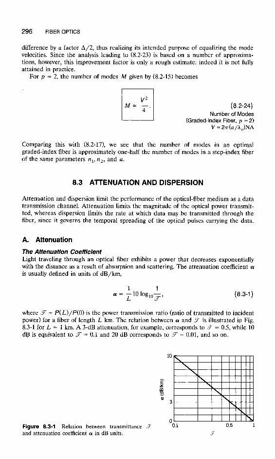
The Attenuation Coefficient Light traveling through an optical fiber exhibits a power that decreases exponentially with the distance as a result of absorption and scattering. The attenuation coefficient (Y is usually defined in units of dB/km,

1 1 a = L 10 logr,y_, (8.3-l)

where 7 = &5)/P(O) is the power transmission ratio (ratio of transmitted to incident power) for a fiber of length L km. The relation between (Y and Y is illustrated in Fig. 8.3-l for L = 1 km. A 3-dB attenuation, for example, corresponds to Y = 0.5, while 10 dB is equivalent to Y = 0.1 and 20 dB corresponds to Y = 0.01, and so on.

Figure 8.3-l Relation between transmittance 7 and attenuation coefficient (Y in dB units.

AlTENUATION AND DISPERSION 297

Losses in dB units are additive, whereas the transmission ratios are multiplicative. Thus for a propagation distance of z kilometers, the loss is (YZ decibels and the power transmission ratio is

P(z) - = P(O)

lo-m/l0 = e-0.23az . (a in dB/km) (8.3-2)

Note that if the attenuation coefficient is measured in km-’ units, instead of in dB/km, then

P(z)/P(O) = e-az (8.3-3)

where cy = 0.23~1. Throughout this section CY is taken in dB/km units so that (8.3-2) applies. Elsewhere in the book, however, we use (Y to denote the attenuation coefficient Cm- ’ or cm-‘) in which case the power attenuation is described by (8.3-3).

Absorption The attenuation coefficient of fused silica glass (SiO,) is strongly dependent on wavelength, as illustrated in Fig. 8.3-2. This material has two strong absorption bands: a middle-infrared absorption band resulting from vibrational transitions and an ultraviolet absorption band due to electronic and molecular transitions. There is a window bounded by the tails of these bands in which there is essentially no intrinsic absorption. This window occupies the near-infrared region.

Scattering Rayleigh scattering is another intrinsic effect that contributes to the attenuation of light in glass. The random localized variations of the molecular positions in glass create random inhomogeneities of the refractive index that act as tiny scattering centers. The amplitude of the scattered field is proportional to 02.+ The scattered intensity is therefore proportional to o4 or to l/At, so that short wavelengths are scattered more than long wavelengths. Thus blue light is scattered more than red (a similar effect, the

Wavelength 1, (pm)

Figure 8.3-2 Dependence of the attenuation coefficient CY of silica glass on the wavelength A,. There is a local minimum at 1.3 pm (cy = 0.3 dB/lun) and an absolute minimum at 1.55 pm (<y = 0.16 dB/km).

‘The scattering medium creates a polarization density 9 which corresponds to a source of radiation proportional to d*~F/dt* = -w*P; see (5.2-19).

298 FIBER OPTICS

Wavelength 1, (pm)

Figure 8.3-3 Ranges of attenuation coefficients of silica glass single-mode and multimode fibers.

scattering of sunlight from tiny atmospheric molecules, is the reason the sky appears blue). The attenuation caused by Rayleigh scattering therefore decreases with wavelength as l/At, a relation known as Rayleigh’s inverse fourth-power law. In the visible band, Rayleigh scattering is more significant than the tail of the ultraviolet absorption band, but it becomes negligible in comparison with infrared absorption for wavelengths greater than 1.6 pm.

The transparent window in silica glass is therefore bounded by Rayleigh scattering on the short-wavelength side and by infrared absorption on the long-wavelength side (as indicated by the dashed lines in Fig. 8.3-2).

Extrinsic Effects In addition to these intrinsic effects there are extrinsic absorption bands due to impurities, mainly OH vibrations associated with water vapor dissolved in the glass and metallic-ion impurities. Recent progress in the technology of fabricating glass fibers has made it possible to remove most metal impurities, but OH impurities are difficult to eliminate. Wavelengths at which glass fibers are used for optical communication are selected to avoid these absorption bands. Light-scattering losses may also be accentu- ated when dopants are added for the purpose of index grading, for example.

The attenuation coefficient of guided light in glass fibers depends on the absorption and scattering in the core and cladding materials, Since each mode has a different penetration depth into the cladding so that rays travel different effective distances, the attenuation coefficient is mode dependent. It is generally higher for higher-order modes. Single-mode fibers therefore typically have smaller attenuation coefficients than multimode fibers (Fig. 8.3-3). Losses are also introduced by small random variations in the geometry of the fiber and by bends.

B. Dispersion

When a short pulse of light travels through an optical fiber its power is “dispersed” in time so that the pulse spreads into a wider time interval. There are four sources of dispersion in optical fibers: modal sion, and nonlinear dispersion.

dispersion, material dispersion, waveguide disper-

ATTENUATION AND DISPERSION 299

Figure 8.3-4 Pulse spreading caused by modal dispersion.

Modal Dispersion Modal dispersion occurs in multimode fibers as a result of the differences in the group velocities of the modes. A single impulse of light entering an M-mode fiber at z = 0 spreads into M pulses with the differential delay increasing as a function of z. For a fiber of length L, the time delays encountered by the different modes are rq = L/u,, q = l,..., M, where uq is the group velocity of mode 4. If U,in and u,, are the smallest and largest group velocities, the received pulse spreads over a time interval L/“min - L/vmax* Since the modes are generally not excited equally, the overall shape of the received pulse is a smooth profile, as illustrated in Fig. 8.3-4. An estimate of the overall rms pulse width is a, = +(L/U,i” - L/u,,). This width represents the response time of the fiber.

In a step-index fiber with a large number of modes, u,,,~ = c,(l - A.) and u,, = c1 (see Sec. 8.1B and Fig. 8.28). Since (1 - A1-l = 1 + A, the response time is

(8.3-4) Response Time

(Multimode Step-Index Fiber)

i.e., it is a fraction A/2 of the delay time L/c,. Modal dispersion is much smaller in graded-index fibers than in step-index fibers

since the group velocities are equalized and the differences between the delay times r4 = L/u, of the modes are reduced. It was shown in Sec. 8.2B and in Fig. 8.2-8 that in a graded-index fiber with a large number of modes and with an optimal index profile, u max = ct and vmin = ci (1 - A2/2>. The response time is therefore

L A2 UT z --

Cl 4’

which is a factor of A/2 smaller than that in a step-index fiber.

(8.3-5) Response Time

(Graded-Index Fiber)

EXAMPLE 8.3-l. Multimode Pulse Broadening Rate. In a step-index fiber with A = 0.01 and n = 1.46, pulses spread at a rate of approximately u,/L = A/2c, = nw% == 24 ns/km. In a loo-km fiber, therefore, an impulse spreads to a width of = 2.4 ps. If the same fiber is optimally index graded, the pulse broadening rate is approximately n,A2/4c, = 122 ps/km, which is substantially reduced.

300 FIBER OPTICS

The pulse broadening arising from modal dispersion is proportional to the fiber length L in both step-index and graded-index fibers. This dependence, however, does not necessarily hold when the fibers are longer than a certain critical length because of mode coupling. Coupling occurs between modes of approximately the same propagation constants as a result of small imperfections in the fiber (random irregularities of the fiber surface, or inhomogeneities of the refractive index) which permit the optical power to be exchanged between the modes. Under certain conditions, the response time a7 of mode-coupled fibers is proportional to L for small L and to L1i2 when a critical length is exceeded, so that pulses are broadened at a slower rate+.

Material Dispersion Glass is a dispersive medium; i.e, its refractive index is a function of wavelength. As discussed in Sec. 5.6, an optical pulse travels in a dispersive medium of refractive index n with a group velocity u = co/N, where N = n - A, dn/dh,. Since the pulse is a wavepacket, composed of a spectrum of components of different wavelengths each traveling at a different group velocity, its width spreads. The temporal width of an optical impulse of spectral width ah (nm), after traveling a distance L, is c7 = I(d/dh,Xl/u)lo, = l(d/dAo)(LN/c,)(aA, from which

where

A, d2n DA= --2 CcJ dh

(8.3-7)

is the material dispersion coefficient [see (5.6-21)]. The response time increases linearly with the distance L. Usually, L is measured in km, a7 in ps, and ah in nm, so that D, has units of ps/km-nm. This type of dispersion is called material dispersion (as

opposed to modal dispersion). The wavelength dependence of the dispersion coefficient D, for silica glass is shown

in Fig. 8.3-5. At wavelengths shorter than 1.3 pm the dispersion coefficient is negative,

40

0

a i?lJ< - 120 w : - 160

0.6 0.7 0.8 0.9 1.0 1.1 1.2 1.3 1.4 1.5 1.6

Wavelength A0 (pm)

Figure 8.3-5 The dispersion coefficient D, of silica glass as a function of wavelength A, (see also Fig. 5.6-5).

‘See, e.g., J. E. Midwinter, Optical Fibers for Transmission, Wiley, New York, 1979.


so that wavepackets of long wavelength travel faster than those of short wavelength. At a wavelength h, = 0.87 pm, the dispersion coefficient D, is approximately -80 ps/km-nm. At A, = 1.55 pm, D, = + 17 ps/km-nm. At A, = 1.312 pm the dispersion coefficient vanishes, so that o7 in (8.3-6) vanishes. A more precise expression for a7 that incorporates the spread of the spectral width oh about A, = 1.312 pm yields a very small, but nonzero, width.

EXAMPLE 8.3-2. Pulse Broadening Associated with Material Dispersion. The dispersion coefficient D, = -80 ps/km-nm at A, = 0.87 pm. For a source of linewidth ah = 50 nm (from an LED, for example) the pulse spreading rate in a single-mode fiber with no other sources of dispersion is [D,[u~ = 4 ns/km. An impulse of light traveling a distance L = 100 km in the fiber is therefore broadened to a width a7 = ID,la,L = 0.4 ps. The response time of the fiber is then 0.4 us. An impulse of narrower linewidth uA = 2 nm (from a laser diode, for example) operating near 1.3 pm, where the dispersion coefficient is 1 ps/km-nm, spreads at a rate of only 2 ps/km. A loo-km fiber thus has a substantially shorter response time, Us = 0.2 ns.

Waveguide Dispersion The group velocities of the modes depend on the wavelength even if material dispersion is negligible. This dependence, known as waveguide dispersion, results from the dependence of the field distribution in the fiber on the ratio between the core radius and the wavelength (a/A,). If this ratio is altered, by altering h,, the relative portions of optical power in the core and cladding are modified. Since the phase velocities in the core and cladding are different, the group velocity of the mode is altered. Waveguide dispersion is particularly important in single-mode fibers, where modal dispersion is not exhibited, and at wavelengths for which material dispersion is small (near A, = 1.3 pm in silica glass).

As discussed in Sec. 8.1B, the group velocity u = (dp/do)-’ and the propagation constant /3 are determined from the characteristic equation, which is governed by the fiber V parameter V = 2r(a/h,)NA = (a * NA/c,)o. In the absence of material dispersion (i.e., when NA is independent of o), V is directly proportional to w, so that

1 dP dp dV a*NA dp -=-c--E-- u do dVdw c, dV’

(8.3-8)

The pulse broadening associated with a source of spectral width uA is related to the time delay L/v by a7 = I(d/dh,XL/u)l~,. Thus

where

(8.3-10)

302 FIBER OPTICS

is the waveguide dispersion coefficient. Substituting (8.3-8) into (8.3-10) we obtain

(8.3-11)

Thus the group velocity is inversely proportional to dp/dV and the dispersion coefficient is proportional to V* d *p/d” *. The dependence of p on V is shown in Fig. 8.1-10(b) for the fundamental LP,, mode. Since p varies nonlinearly with V, the waveguide dispersion coefficient Dw is itself a function of V and is therefore also a function of the wavelength. + The dependence of D, on A, may be controlled by altering the radius of the core or the index grading profile for graded-index fibers.

Combined Material and Waveguide Dispersion The combined effects of material dispersion and waveguide dispersion (referred to here as chromatic dispersion) may be determined by including the wavelength dependence of the refractive indices, nl and n2 and therefore NA, when determining dp/dw from the characteristic equation. Although generally smaller than material dispersion, waveguide dispersion does shift the wavelength at which the total chromatic dispersion is minimum.

Since chromatic dispersion limits the performance of single-mode fibers, more advanced fiber designs aim at reducing this effect by using graded-index cores with refractive-index profiles selected such that the wavelength at which waveguide dispersion compensates material dispersion is shifted to the wavelength at which the fiber is to be used. Dispersion-shifted fibers have been successfully made by using a linearly tapered core refractive index and a reduced core radius, as illustrated in Fig. 8.3-6(a). This technique can be used to shift the zero-chromatic-dispersion wavelength from 1.3 pm to 1.55 pm, where the fiber has its lowest attenuation. Note, however, that the process of index grading itself introduces losses since dopants are used. Other grading profiles have been developed for which the chromatic dispersion vanishes at two wavelengths and is reduced for wavelengths between. These fibers, called dispersion- flattened, have been implemented by using a quadruple-clad layered grading, as illustrated in Fig. 8.3-6(b).

Combined Material and Modal Dispersion The effect of material dispersion on pulse broadening in multimode fibers may be determined by returning to the original equations for the propagation constants p, of the modes and determining the group velocities uq = (dp,/do)-’ with n1 and n2 being functions of o. Consider, for example, the propagation constants of a graded- index fiber with a large number of modes, which are given by (8.2-19) and (8.2-15). Al- though n, and n2 are dependent on o, it is reasonable to assume that the ratio A = (n, - n2)/nl is approximately independent of o. Using this approximation and evalu- ating uq = (d/3Jdo)-‘, we obtain

(8.3-12)

where N, = (d/do)(wnl) = n1 - A,(dn,/dh,) is the group index of the core material. Under this approximation, the earlier expression (8.2-21) for vq remains the same, except that the refractive index n, is replaced with the group index Nr. For a step-index fiber (p = m), the group velocities of the modes vary from c,/Nr to

’ For more details on this topic, see the reading list, particularly the articles by Gloge.


Cladding

: Core -+P--

a

0 -- n

a

n

Figure 8.3-6 Refractive-index profiles and schematic wavelength dependences of the material dispersion coefficient (dashed curves) and the combined material and waveguide dispersion coefficients (solid curves) for (a) dispersion-shifted and (b) dispersion-flattened fibers.

(co/NIX1 - A), so that the response time is

L A

ar = (co/N,) -!i-’ (8.3-13)

Response Time (Multimode Step-Index Fiber

with Material Dispersion)

This should be compared with (8.3-4) when there is no material dispersion.

EXERCISE 8.3- 1

Optimal Grade Profile Parameter. Use (8.2-19) and (8.2-E) to derive the following expression for the group velocity uq when both n1 and A are wavelength dependent:

vq ( ;)P”“+2’A], q = 1,2,. . . , M, (8.3-14)

where ps = 2(nr/NrXo/A) dA/d w. What is the optima1 value of the grade profile parameter p for minimizing modal dispersion?

Nonlinear Dispersion Yet another dispersion effect occurs when the intensity of light in the core is sufficiently high, since the refractive indices then become intensity dependent and the material exhibits nonlinear behavior. The high-intensity parts of an optical pulse undergo phase shifts different from the low-intensity parts, so that the frequency is shifted by different amounts. Because of material dispersion, the group velocities are

304 FIBER OPTICS

modified, and consequently the pulse shape is altered. Under certain conditions, nonlinear dispersion can compensate material dispersion, so that the pulse travels without altering its temporal profile. The guided wave is then known as a solitary wave, or a soliton. Nonlinear optics is introduced in Chap. 19 and optical solitons are discussed in Sec. 19.8.

C. Pulse Propagation

As described in the previous sections, the propagation of pulses in optical fibers is governed by attenuation and several types of dispersion. The following is a summary and recapitulation of these effects, ignoring nonlinear dispersion.

An optical pulse of power ~;$(t/r,,) and short duration ro, where p(t) is a function which has unit duration and unit area, is transmitted through a multimode fiber of length L. The received optical power may be written in the form of a sum

P(t) a f exp( -0.23ol,L)u;‘p ~ t - Tq

( I ,

q=l %

(8.3-15)

where M is the number of modes, the subscript q refers to mode q, aq is the attenuation coefficient (dB/km), rs = L/u, is the delay time, uq is the group velocity, and a4 > 7. is the width of the pulse associated with mode q. In writing (8.3-H), we have implicitly assumed that the incident optical power is distributed equally among the M modes of the fiber. It has also been assumed that the pulse shape p(t) is not altered; it is only delayed by times rq and broadened to widths as as a result of propagation. As was shown in Sec. 5.6, an initial pulse with a Gaussian profile is indeed broadened without altering its Gaussian nature.

The received pulse is thus composed of M pulses of widths gq centered at time delays rq, as illustrated in Fig. 8.3-7. The composite pulse has an overall width a7 which represents the overall response time of the fiber.

We therefore identify two basic types of dispersion: intermodal and intramodal. Intermodal, or simply modal, dispersion is the delay distortion caused by the disparity among the delay times 7q of the modes. The time difference +(T,, - Ten) between the longest and shortest delay constitutes modal dispersion. It is given by (8.3-4) and (8.3-5) for step-index and graded-index fibers with a large number of modes, respectively. Material dispersion has some effect on modal dispersion since it affects the delay times. For example, (8.3-13) gives the modal dispersion of a multimode fiber with material dispersion. Modal dispersion is directly proportional to the fiber length L, except for long fibers, in which mode coupling plays a role, whereupon it becomes proportional to L’12.

Intramodal dispersion is the broadening of the pulses associated with the individual modes. It is caused by a combination of material dispersion and waveguide dispersion

Figure 8.3-7 Response of a multimode fiber to a single pulse.

ATTENUATION AND DISPERSION 305

Multimode step-index fiber

I Ll 0 t

Graded-index fiber

Multimode step-index fiber (coupled modes)

L Ll 0 t

Single-mode fiber

L Ll 0 t

Nonlinear fiber

Ld!L 0 t

?a

I 0

!!L UT t

Soliton L 0 t

Figure 8.3-8 Broadening of a short optical pulse after transmission through different types of fibers. The width of the transmitted pulse is governed by modal dispersion in multimode (step-index and graded-index) fibers. In single-mode fibers the pulse width is determined by material dispersion and waveguide dispersion. Under certain conditions an intense pulse, called a soliton, can travel through a nonlinear fiber without broadening. This is a result of a balance between material dispersion and self-phase modulation (the dependence of the refractive index on the light intensity).

306 FIBER OPTICS

resulting from the finite spectral width of the initial optical pulse. The width a4 is given by

a4 2 = r; -I- (DqcALj2, (8.3-16)

where Dq is a dispersion coefficient representing the combined effects of material and waveguide dispersion for mode q. Material dispersion is usually more significant. For a very short initial width TV, (8.3-16) gives

aq = DquAL. (8.3-17)

Figure 8.3-8 is a schematic illustration in which the profiles of pulses traveling through different types of fibers are compared. In multimode step-index fibers, the modal dispersion i(r,, - 7,in) is usually much greater than the material/waveguide dispersion as, so that intermodal dispersion dominates and a7 = i(r,, - 7,in). In multimode graded-index fibers, i(~,, - 7,in) may be comparable to us, so that the overall pulse width involves all dispersion effects. In single-mode fibers, there is obviously no modal dispersion and the transmission of pulses is limited by material and waveguide dispersion. The lowest overall dispersion is achieved in a single-mode fiber operating at the wavelength for which the combined material-waveguide dispersion vanishes.

READING LIST

Books See also the books on optical waveguides in Chapter 7. P. K. Cheo, Fiber Optics and Optoelectronics, Prentice Hall, Englewood Cliffs, NJ, 1985, 2nd ed.

1990. F. C. Allard, Fiber Optics Handbook for Engineers and Scientists, McGraw-Hill, New York, 1990. C. Yeh, Handbook of Fiber Optics: Theory and Applications, Academic Press, Orlando, FL, 1990. L. B. Jeunhomme, Single-Mode Fiber Optics, Marcel Dekker, New York, 1983, 2nd ed. 1990. P. W. France, ed., Fluoride Glass Optical Fibers, CRC Press, Boca Raton, FL, 1989. P. Diament, Wave Transmission and Fiber Optics, Macmillan, New York, 1989. W. B. Jones, Jr., Introduction to Optical Fiber Communication Systems, Holt, Rinehart and

Winston, New York, 1988. H. Murata, Handbook of Optical Fibers and Cables, Marcel Dekker, New York, 1988. E. G. Neuman, Single-Mode Fibers-Fundamentals, Springer-Verlag, New York, 1988. E. L. Safford, Jr. and J. A. McCann, Fiberoptics and Laser Handbook, Tab Books, Blue Ridge

Summit, PA, 2nd ed. 1988. S. E. Miller and I. Kaminow, Optical Fiber Telecommunications II, Academic Press, Boston, MA,

1988. J. Gowar, Optical Communication Systems, Prentice Hall, Englewood Cliffs, NJ, 1984. R. G. Seippel, Fiber Optics, Reston Publishing, Reston, VA, 1984. ANSI/IEEE Standards 812-1984, IEEE Standard Definitions of Terms Relating to Fiber Optics,

IEEE, New York, 1984. A. H. Cherin, An Introduction to Optical Fibers, McGraw-Hill, New York, 1983. G. E. Keiser, Optical Fiber Communications, McGraw-Hill, New York, 1983. C. Hentschel, Fiber Optics Handbook, Hewlett-Packard, Palo Alto, CA, 1983. Y. Suematsu and K. Iga, Introduction to Optical Fiber Communications, Wiley, New York, 1982. T. Okoshi, Optical Fibers, Academic Press, New York, 1982. C. K. Kao, Optical Fiber Systems, McGraw-Hill, New York, 1982. E. A. Lacy, Fiber Optics, Prentice-Hall, Englewood Cliffs, NJ, 1982.

PROBLEMS 307

D. Marcuse, Light Transmission Optics, Van Nostrand Reinhold, New York, 1972, 2nd ed. 1982. D. Marcuse, Principles of Optical Fiber Measurements, Academic Press, New York, 1981. A. B. Sharma, S. J. Halme, and M. M. Butusov, Optical Fiber Systems and Their Components,

Springer-Verlag, Berlin, 1981. CSELT (Centro Studi e Laboratori Telecomunicazioni), Optical Fibre Communications,

McGraw-Hill, New York, 1981. M. K. Barnoski, ed., Fundamentals of Optical Fiber Communications, Academic Press, New York,

1976, 2nd ed. 1981. C. P. Sandbank, ed., Optical Fibre Communication Systems, Wiley, New York, 1980. M. J. Howes and D. V. Morgan, eds., Optical Fibre Communications, Wiley, New York, 1980. H. F. Wolf, ed., Handbook of Fiber Optics, Garland STPM Press, New York, 1979. D. B. Ostrowsky, ed., Fiber and Integrated Optics, Plenum Press, New York, 1979. J. E. Midwinter, Optical Fibers for Transmission, Wiley, New York, 1979. S. E. Miller and A. G. Chynoweth, Optical Fiber Telecommunications, Academic Press, New York,

1979. G. R. Elion and H. A. Elion, Fiber Optics in Communication Systems, Marcel Dekker, New York,

1978. H. G. Unger, Planar Optical Waveguides and Fibers, Clarendon Press, Oxford, 1977. J. A. Arnaud, Beam and Fiber Optics, Academic Press, New York, 1976. W. B. Allan, Fibre Optics: Theory and Practice, Plenum Press, New York, 1973. N. S. Kapany, Fiber Optics: Principles and Applications, Academic Press, New York, 1967.

Special Journal Issues Special issue on fiber-optic sensors, Journal of Lightwaue Technology, vol. LT-5, no. 7, 1987. Special issue on fiber, cable, and splicing technology, Journal of Lightwave Technology, vol. LT-4,

no. 8, 1986. Special issue on low-loss fibers, Journal of Lightwaue Technology, vol. LT-2, no. 10, 1984. Special issue on fiber optics, IEEE Transactions on Communications, vol. COM-26, no. 7, 1978.

Articles M. G. Drexhage and C. T. Moynihan, Infrared Optical Fibers, Scientific American, vol. 259, no. 5,

pp. 110-114, 1988. S. R. Nagel, Optical Fiber-the Expanding Medium, IEEE Communications Magazine, vol. 25,

no. 4, pp. 33-43, 1987. R. H. Stolen and R. P. DePaula, Single-Mode Fiber Components, Proceedings of the IEEE, vol.

75, pp. 1498-1511, 1987. P. S. Henry, Lightwave Primer, IEEE Journal of Quantum Electronics, vol. QE-21, pp. 1862-1879,

1985. T. Li, Advances in Optical Fiber Communications: An Historical Perspective, IEEE Journal on

Selected Areas in Communications, vol. SAC-l, pp. 356-372, 1983. I. P. Kaminow, Polarization in Optical Fibers, IEEE Journal of Quantum Electronics, vol. QE-17,

pp. 15-22, 1981. P. J. B. Clarricoats, Optical Fibre Waveguides-A Review, in Progress in Optics, vol. 14, E. Wolf,

ed., North-Holland, Amsterdam, 1977. D. Gloge, Weakly Guiding Fibers, Applied Optics, vol. 10, pp. 2252-2258, 1971. D. Gloge, Dispersion in Weakly Guiding Fibers, Applied Optics, vol. 10, pp. 2442-2445, 1971.

8.1-1 Coupling Efficiency. (a) A source emits light with optical power P, and a distribution I(0) = (l/r)/‘, cos 8, where I(0) is the power per unit solid angle in the direction making an angle 8 with the axis of a fiber. Show that the power collected

308

8.1-2

8.1-3

8.1-4

8.2-l

8.2-2

8.2-3

8.3-l

8.3-2

8.3-3

FIBER OPTICS

by the fiber is P = (NA)*P,, i.e., the coupling efficiency is NA* where NA is the numerical aperture of the fiber. (b) If the source is a planar light-emitting diode of refractive index n, bonded to the fiber, and assuming that the fiber cross-sectional area is larger than the LED emitting area, calculate the numerical aperture of the fiber and the coupling efficiency when n, = 1.46, n2 = 1.455, and n, = 3.5.

Modes. A step-index fiber has radius a = 5 pm, core refractive index n1 = 1.45, and fractional refractive-index change A = 0.002. Determine the shortest wavelength A, for which the fiber is a single-mode waveguide. If the wavelength is changed to A,/2, identify the indices (I, m) of all the guided modes.

Modal Dispersion. A step-index fiber of numerical aperture NA = 0.16, core radius a = 45 pm and core refractive index n, = 1.45 is used at A, = 1.3 pm, where material dispersion is negligible. If a pulse of light of very short duration enters the fiber at t = 0 and travels a distance of 1 km, sketch the shape of the received pulse: (a) Using ray optics and assuming that only meridional rays are allowed. (b) Using wave optics and assuming that only meridional (1 = 0) modes are allowed.

Propagation Constants and Group Velocities. A step-index fiber with refractive indices n, = 1.444 and n2 = 1.443 operates at A, = 1.55 pm. Determine the core radius at which the fiber V parameter is 10. Use Fig. 8.1-6 to estimate the propagation constants of all the guided modes with 1 = 0. If the core radius is now changed so that V = 4, use Fig. 8.1-10(b) to determine the propagation constant and the group velocity of the LPO, mode. Hint: Derive an expression for the group velocity u = (d/3/&)-l in terms of dp/dV and use Fig. 8.1-10(b) to estimate d/?/N. Ignore the effect of material dispersion.

Numerical Aperture of a Graded-Index Fiber. Compare the numerical apertures of a step-index fiber with n, = 1.45 and A = 0.01 and a graded-index fiber with n , = 1.45, A = 0.01, and a parabolic refractive-index profile (p = 2). (See Exercise 1.3-2 on page 24.)

Propagation Constants and Wavevector (Step-Index Fiber). A step-index fiber of radius a = 20 pm and refractive indices n, = 1.47 and n2 = 1.46 operates at A, = 1.55 pm. Using the quasi-plane wave theory and considering only guided modes with azimuthal index I = 1: (a) Determine the smallest and largest propagation constants. (b) For the mode with the smallest propagation constant, determine the radii of the cylindrical shell within which the wave is confined, and the components of the wavevector k at r = 5 pm.

Propagation Constants and Wavevector (Graded-Index Fiber). Repeat Problem 8.2-2 for a graded-index fiber with parabolic refractive-index profile with p = 2.

Scattering Loss. At A, = 820 nm the absorption loss of a fiber is 0.25 dB/km and the scattering loss is 2.25 dB/km. If the fiber is used instead at A, = 600 nm and calorimetric measurements of the heat generated by light absorption give a loss of 2 dB/km, estimate the total attenuation at A, = 600 nm.

Modal Dispersion in Step-Index Fibers. Determine the core radius of a multimode step-index fiber with a numerical aperture NA = 0.1 if the number of modes M = 5000 when the wavelength is 0.87 pm. If the core refractive index n, = 1.445, the group index N, = 1.456, and A is approximately independent of wavelength, determine the modal-dispersion response time a7 for a 2-km fiber.

Modal Dispersion in Graded-Index Fibers. Consider a graded-index fiber with a/A, = 10. n, = 1.45. A = 0.01, and a power-law profile with index u. Determine

PROBLEMS 309

8.3-4

the number of modes M, and the modal-dispersion pulse-broadening rate u,/L for p = 1.9, 2, 2.1, and m.

Pulse Propagation, A pulse of initial width TV is transmitted through a graded-index fiber of length L kilometers and power-law refractive-index profile with profile index p. The peak refractive index n, is wavelength-dependent with D, = -(&/c,)d2nl/dh2,, A is approximately independent of wavelength, ah is the source’s spectral width, and h, is the operating wavelength. Discuss the effect of increasing each of the following parameters on the width of the received pulse: L, TV, P, IDAl, q, and A,.

FIBER OPTICS -...

Documents

Transcript of FIBER OPTICS -...