Factors Affecting Demand Amplification in Supply Chains · Factors Affecting Demand Amplification...

Factors Affecting Demand Amplification in Supply Chains (Abstract Number: 003-0073)

Sixteenth Annual Conference of POMS Chicago, IL, April 29 – May 2, 2005

Seung-Kuk Paik, Ph.D. Assistant Professor

Systems and Operations Management Department College of Business and Economics

California State University, Northridge 18111 Nordhoff Street

Northridge, CA 91330-8378 Email: [email protected]

Phone: 818-677-4627 Fax: 818-677-6079

2

Abstract

Using computer simulation models, this study investigates the factors that are

believed to affect demand amplification and examines their effects on the variability of

orders in supply chains. When there are multiple levels of echelons in the supply chains,

information sharing and coordination within and across the organizations are essential to

reduce demand amplification. Sharing of accurate demand information leads to a better

matching of supply and demand so that mismatch cost between supply and demand can be

reduced. When few intermediaries are involved in a supply chain, a factory’s activities tend

to fluctuate as the actual demand changes. Market responsiveness or agility is a useful

principle to dampen the bullwhip effect when there are few intermediaries involved in a

supply chain.

Introduction

Supply chain management emphasizes close coordination among the various

companies involved in the chain (Lambert et al., 1998; Christopher, 1998; Bowersox et al.,

2003). Unless there is a good coordination among the supply chain members, it causes

many problems in the supply chain and consequently weakens the effectiveness of the

3

whole supply chain. The bullwhip effect is a well-known example of supply chain

dynamics when there is no or little coordination among the supply chain members. Since

Forrester (1958; 1961) first discussed the amplification of demand in a supply chain using a

simulation model, many researchers have investigated the bullwhip effect. Although some

research has been done to examine the bullwhip effect in intra-organizational echelons

(Svensson, 2003), the majority of research has concentrated on the bullwhip effect in inter-

organizational structures (Sterman, 1989; Lee et al., 1997; Hong-Minh et al., 2000; Chen

and Samroengraja, 2000; McCullen and Towill, 2001; Yu et al., 2001).

Although many previous studies have identified several possible causes of the

bullwhip effect, little attention was given to the measurement of the bullwhip effect based

on the causes identified in the previous literature. Most of the past work acknowledged the

existence of the bullwhip effect and enumerated the possible causes. But many of the past

studies failed to accurately investigate the relative contribution of each of the causes of

bullwhip effect. In particular, there is little research addressing the severity of demand

amplification under different supply chain structures. This study seeks to fill this gap by

incorporating and analyzing the set of the causes of the bullwhip effect in computer

simulation models. By building and running computer simulation models with the variables

4

corresponding to the various causes, this study investigates each of the causes and seeks to

determine their relative effects on the demand amplification under each of three different

supply chain structures. By examining the effects on multiple supply chain structures, this

study tries to help business practitioners find out a more effective approach to mitigate the

demand amplification. More specifically, this study seeks to achieve the following research

objectives:

• To examine the aggregate impact of the set of causes of the bullwhip effect on

the variability of orders under three different supply chain structures.

• To determine the relative contribution of each cause of the bullwhip effect on

the variability of orders under three different supply chain structures.

This study takes nine causes of the bullwhip effect identified in previous studies and

examines the aggregate effect of the nine causes on the bullwhip effect. After determining

the overall impact of the selected causes, this study assesses the relative contribution of

each cause on the variability of orders under different supply chain structures. Based on the

relative contribution measured, it determines which cause has the most significant effect on

the bullwhip effect.

5

Research Methodology

The main research methodologies used in this study include computer simulation

and statistical analysis. The purpose of computer simulation is to obtain data of order

quantities placed by each of the participants in supply chains, while the statistical technique

is to analyze the obtained data and present findings related to the research objectives.

Because this research investigates the causes of the bullwhip effect under three

different supply chain structures, it requires building simulation models representing

different supply chain systems. The Beer Distribution Game is used as a benchmark model

representing a supply chain. Nine causes of the bullwhip effect are incorporated as the

variables in the simulation models, as shown in Table 1. By changing the value of the nine

variables, this study seeks to investigate the relationship between each of the causes and the

severity of its effect on the bullwhip effect.

Table 1. Relationship between the Causes and the Variables

Causes of the Bullwhip Effect Corresponding Concept Variables in the Simulation

Demand forecast updates Level of safety stock Correction (αs) factor for any shortfall of inventory

Order batching Timing of batch Time interval btw. order batch (OB)

Shortage and rationing gaming

Multiple ordering Ratio (β) of correction factor for orders and goods in transit to αs

Material lead-time Material delay Transportation delay (MD)

6

Information lead-time Information delay Order & mail delay (ID)

Capacity limit Maximum capacity Upper capacity limit (CL)

Machine breakdown Production delay Delay in production (PD)

Price variation Average waiting time before purchasing

Delay in purchasing (PDC)

Level of echelons Number of echelons Number of echelons (LE)

These nine variables are used to predict the level of the amplification of order as the

dependent variable in the statistical analysis. This study measures amplification factor as a

proxy variable for the variability of orders in a supply chain during the experiments. The

amplification factor is measured in the excursion (∆ factory order) of the output variable

relative to that (∆ customer order) of the input (Sterman, 1989).

For data collection, a factorial arrangement with nine factors each at three levels is

proposed, and a complete factorial experiment requires 39 = 19,683 runs. But since the

number of runs required is so large that it is not economical to carry out the complete

factorial experiment, fractional factorial design is used. In this study, a fraction (1/81) or

3(9-4) fractional factorial design is constructed in order to investigate the main effect of each

of the selected causes of the bullwhip effect (Conner and Zelen, 1959; Montgomery, 1991).

This fractional factorial experiment requires 243 observations.

The outcomes of the simulations do not speak for themselves. Simulation often

7

requires some statistical techniques to analyze and present the results of the computer

simulation models. The analysis of variance is most commonly used in simulations

designated to probe the impacts of several independent variables on a single dependent

variable (Whicker and Sigelman, 1991). The objective of the analysis of variance for

fractional factorial experiments is to examine the effects of two or more factors on the

dependent variable, whether or not interaction exists.

After this study determines the aggregate impact of the selected causes, it then

assesses the relative contribution of each of the causes on the variability of orders in supply

chains. In this assessment, the causes of the bullwhip effect are ranked based on their

relative contributions, which can be measured by partial R-squares. The rank tells us which

cause of the bullwhip effect has the most significant impact on the variability of orders in

supply chains. All of the observations collected from the simulation runs are divided into

different groups, depending on the number of echelons. In this study, three different supply

chain structures are investigated to understand the causes of the bullwhip effect. For each of

these groups, the aggregate impact and the relative contribution of the causes of the

bullwhip effect are examined to provide managerial implications.

8

Capturing Decision-Makers’ Behavioral Pattern

Any modeling approach, including simulation, is often believed to suffer from

external validity (Mentzer and Flint, 1997). External validity indicates whether the research

findings can be generalized. The external validity of a computer simulation model depends

on both how well a logic underlying the model reflects the underlying phenomena and how

well the computer program represents the model (Whicker and Sigelman, 1991).

In order to capture the behavioral pattern of real decision-makers, several sessions

of the Beer Distribution Game were conducted with undergraduate and graduate students,

including executive MBA students, at two universities – the George Washington University

and the University of California, Riverside. Many of the graduate students who participated

in the games are responsible business managers who make important business decisions for

their organizations. Using the data collected from the various sessions of the game, pattern

matching was conducted to ensure the validity of the computer model. If a pattern similar to

the one found in the Beer Distribution Game is detected in the computer models, then the

computer models are believed to reflect the underlying behavioral pattern of decision-

makers (Whicker and Sigelman, 1991).

9

When collecting all of 243 observations, the behavioral pattern of the computer

model was observed to see whether there is any major departure from the expected pattern

or whether any unusual outputs are received. None of these was found in the simulation

models. Figure 1 illustrates the ordering pattern by each of the supply chain members when

there are four levels of echelon in a supply chain. This figure was drawn from the data

generated by the simulation model.

Figure 1. Ordering Pattern in a Computer Simulation Model

Order Rate

0

5

10

15

20

25

30

35

week

orde

r rat

e RetailerWholesalerDistributorFactory

The computer simulation models exhibited the three distinctive characteristics of the

bullwhip effect: oscillation, amplification, and phased time lags on order level in the supply

10

chain. Order quantities were oscillated in either direction and showed excessive swings.

Second, the amplification of orders increased steadily from retailer to factory. Third, the

order quantities peaked later as the orders moved from the downstream members to the

upstream members.

Along with this pattern matching, this study compared the ordering patterns of the

real decision makers and those of the computer simulation model. As shown in Figure 2,

similar ordering behavior could be observed in each of the supply chain members, although

the magnitudes of the order quantities were different.

Figure 2. Comparison Between Actual Decision Maker’s Behavior and Computer Simulation Model

0

10

20

30

40

50

1 7 13 19 25 31

DecisionM aker

Simulat ionM odel

Retailer

0

10

20

30

40

50

1 6 11 16 21 26 31

DecisionMaker

SimulationModel

Wholesaler

11

0

10

20

30

40

50

1 7 13 19 25 31

DecisionM aker

Simulat ionM odel

Distributor

0

10

20

30

40

50

1 6 11 16 21 26 31

DecisionMaker

SimulationModel

Factory

Impact of the Variables on the Bullwhip Effect Under Different Supply Chain

Structures

The number of echelon is one of the significant factors causing the bullwhip effect

in a supply chain (Towill, et al., 1992; Ackere et al., 1993; Evans et al., 1993). Depending

on the number of echelon, three different supply chain structures are investigated in the

study. In each of these supply chain structures, the effects of the variables on demand

amplification are examined to understand their relative contributions on the bullwhip effect.

Four Levels of Echelons

Table 2 provides a summary of the statistical analysis when there are four

participants in the supply chain, which includes retailer, wholesaler, distributor and factory.

Because the p-value (p-value < 0.0001) of this model is less than the predetermined alpha

12

value (α = 0.05), we are at least 95 percent confident that the set of the causes predicts

some variations in the values of demand amplification factor. The overall model R-square

is 0.9283, indicating that 92.83% of the variations in the demand amplification factor can

be explained by the set of the selected variables in the model.

Regarding each of the selected independent variables, five independent variables are

statistically significant. These five independent variables include alpha (αs), order batching,

material delay, information delay, and purchasing delay. As shown in Table 2, “alpha” for

demand forecast updating is the most significant factor among the selected variables,

followed by purchasing delay for price variation, order batching, material delay and

information delay. However, "beta" (β) for rationing and shortage gaming, capacity limit

for production constraint, and production delay for supply variability are not statistically

significant with α = 0.05.

Table 2. Impact of the Causes of the Bullwhip Effect at Four Echelons

Variables F-value P-value R-square Rank

Model 15.81 <0.0001 92.83%

Alpha(ALPHA) 120.98 <0.0001 39.45% 1

13

Order Batching (OB) 24.24 <0.0001 7.90% 3

Beta (BETA) 0.64 0.5307 0.21% N.S.

Material Delay (MD) 14.04 <0.0001 4.58% 4

Information Delay (ID) 11.95 <0.0001 3.90% 5

Capacity Limit (CL) 1.12 0.3358 0.36% N.S.

Production Delay (PD) 0.16 0.8500 0.05% N.S.

Purchasing Delay (PDC) 52.77 <0.0001 17.21% 2

ALPHA×MD 6.78 0.0027 2.21%

ALPHA×ID 5.67 0.0064 1.85%

ALPHA×PDC 9.73 <0.0001 6.35%

OB×PDC 3.46 0.0153 2.26%

N.S.: Not significant

Ranks are made only on the main effects

When there are four levels of echelon in a supply chain, the following interaction

variables, ALPHA×MD, ALPHA×ID, ALPHA×PDC, and OB×PDC, are statistically

significant, and thus, it is important to determine whether there are ordinal relationships

between the variables. If there are disorderly interactions between the variables, it can

obscure the main effects and thus may be impossible to directly examine them. Orderly

interaction exists between two factors when the order of the means for levels of one factor

14

is always the same even though the magnitude of the differences between levels of the

factor may change from level to level of the other factor. Although ALPHA×PDC and

OB×PDC do not show any disordinal relationship, ALPHA×MD and ALPHA×ID show

disorderly relationship between the factors.

For the ALPHA×MD variable, disorderly relationship is detected only between a

one-week and a two-week material delay (MD) at ALPHA = 0.13. Other than this, no

disordinal relationship is found in any other combination of these two factors. Regarding

the main effects on the material delay (MD), there is no statistical significance between a

one-week and a two-week delay, as shown in the following table.

Table 2.1. Scheffe Test for “MD”

Scheffe Grouping* Mean N Level

A 1,611.4 27 4

B 1,150.0 27 2

B 1,017.0 27 1

*: Means with the same letter are not significantly different.

The ALPHA×ID variable also shows disorderly relationship only between a one-

week and a two-week information delay (ID) at ALPHA = 0.26. Other than this, no

15

disordinal relationship is found in any other combination of the two factors. Regarding the

main effects on the information delay (ID), statistical significance is not found between a

one-week and a two-week delay.

Table 2.2. Scheffe Test for “ID”


A 1,588.3 27 4

B 1,136.7 27 2

B 1,053.4 27 1


Three Levels of Echelons

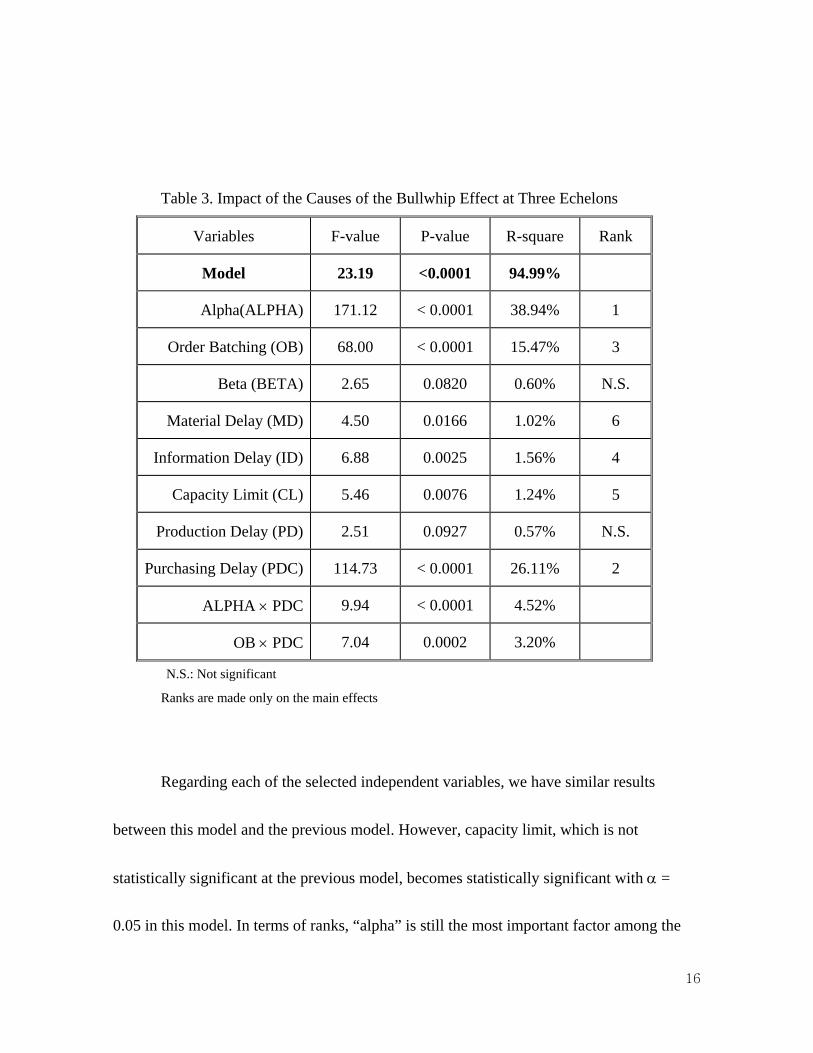
Table 3 shows the results under three levels of echelons, including retailer,

distributor and factory. The overall model is statistically significant with α = 0.05 (p-value

< 0.0001). Therefore, we are at least 95 percent confident that the set of the selected causes

predicts some variation in the values of demand amplification factor. The overall model R-

square is 0.9499, indicating that 94.99% of the variation in the demand amplification factor

can be explained by the set of the selected variables in the model.

16

Table 3. Impact of the Causes of the Bullwhip Effect at Three Echelons


Model 23.19 <0.0001 94.99%

Alpha(ALPHA) 171.12 < 0.0001 38.94% 1

Order Batching (OB) 68.00 < 0.0001 15.47% 3

Beta (BETA) 2.65 0.0820 0.60% N.S.

Material Delay (MD) 4.50 0.0166 1.02% 6

Information Delay (ID) 6.88 0.0025 1.56% 4

Capacity Limit (CL) 5.46 0.0076 1.24% 5


Purchasing Delay (PDC) 114.73 < 0.0001 26.11% 2

ALPHA × PDC 9.94 < 0.0001 4.52%

OB × PDC 7.04 0.0002 3.20%



Regarding each of the selected independent variables, we have similar results

between this model and the previous model. However, capacity limit, which is not

statistically significant at the previous model, becomes statistically significant with α =

0.05 in this model. In terms of ranks, “alpha” is still the most important factor among the

17

variables, followed by purchasing delay and order batching. These three main effects

account for about 81 percent of the total variations in the values of demand amplification

factor. The remaining portions are explained by information delay, capacity limit, and

material delay.

In this model, capacity limit is a statistically significant variable. Although its

predictability for the variation in the values of the dependent variable is minimal, only 1.24

percent, it is significant, indicating that this variable provides additional predictability of

the amplification factor above and beyond the predictability offered by the other variables.

For capacity limit, three levels are chosen. During the simulation runs, factory can

produce either 8 beers, 50 beers, or 200 beers per week. A statistically significant

difference exists only between 8 and 200 beers. As shown in Table 3.1, the average demand

amplification factor at eight-beer production capacity is 801.39, compared to 706.20 and

661.76 at 50-beer production capacity and 200-beer production capacity, respectively. As

production capacity decreases, the demand amplification factor increases.

18

Table 3.1. Scheffe Test for Capacity Limit


A 801.39 27 8

A B 706.20 27 50

B 661.76 27 200


In this model, two statistically significant interaction variables, ALPHA × PDC and

OB × PDC, show the ordinal relationship.

Two Levels of Echelons

Table 4 shows the statistical results when there are two levels of echelons in a

supply chain, consisting of only retailer and factory. The overall model is statistically

significant (p-value: < 0.0001). Therefore, we can be at least 95 percent confident that the

set of the selected causes predicts some variation in the values of demand amplification

factor. The overall model R-square is 0.9797, meaning that 97.97% of the variation in the

demand amplification factor can be accounted for by the set of the selected variables in the

model.

19

Table 4. Impact of the Causes of the Bullwhip Effect at Two Echelons


Model 59.09 < 0.0001 97.97%

Alpha(ALPHA) 244.08 < 0.0001 22.48% 3

Order Batching (OB) 266.52 < 0.0001 24.55% 2

Beta (BETA) 4.19 0.0216 0.39% 5

Material Delay (MD) 6.13 0.0045 0.56% 4

Information Delay (ID) 3.47 0.0398 0.32% 6

Capacity Limit (CL) 1.06 0.3559 0.10% N.S.


Purchasing Delay (PDC) 437.80 < 0.0001 40.33% 1

ALPHA × MD 4.26 0.0203 0.39%

ALPHA × PDC 21.82 < 0.0001 4.02%

OB × PDC 21.16 < 0.0001 3.90%



In this model, six independent variables are statistically significant with α = 0.05.

These independent variables include alpha (αs), order batching, beta (β), material delay,

information delay, and purchasing delay. In terms of ranks based on the partial R-square,

these variables show different ranks compared to other results. In this model, when there

20

are only two levels of echelons, purchasing delay is the most significant independent

variable, followed by order batching. “Alpha”, which is the most significant variable in

other analyses, is the third most important contributing factor to demand amplification in

this model. These three important variables are followed by material delay, “beta”, and

information delay. The top three variables can explain about 87 percent of the variations in

the values of demand amplification factor. Capacity limit and production delay are not

statistically significant variables in this model.

In this analysis, the following interaction variables, ALPHA×MD, ALPHA×PDC,

and OB×PDC, are statistically significant. Although ALPHA×PDC and OB×PDC do not

show any disordinal relationship, a disorderly relationship is detected in ALPHA×MD only

between a one-week and a two-week material delay (MD) at ALPHA = 0.26. Once again,

no disordinal relationship was found in any other combination of these two factors.

Regarding the main effects on the material delay (MD), there is no statistical significance

between a one-week and a two-week delay, as shown in the following table.

21

Table 4.1. Scheffe Test for “MD”


A 449.35 27 4

B 413.61 27 2

B 407.22 27 1


Managerial Implication

Multiple Levels of Echelons

When there are multiple levels of echelons in the supply chain, the three most

significant causes of the bullwhip effect are demand forecast updating, purchasing delays

and order batching. These three variables explain at least about 65 percent of the variations

in the demand amplification factor when there are four or three levels of echelons in the

supply chain. In particular, the independent variable for demand forecast updating, "alpha",

is very significant compared to other two variables. As shown in the following table, the

relative contribution of this variable measured in the partial R-square is very high compared

to those of the others.

22

Table 5. Partial R-squares of the Three Variables at Four and Three Echelons

"Alpha" Price Variation Order Batching

Four Echelons 39.45% 17.21% 7.90%

Three Echelons 38.94% 26.11% 15.47%

This result indicates that, when there are multiple levels of echelons, demand

forecast updating is the area on which supply chain managers need to focus in order to

dampen the bullwhip effect. What demand forecast updating implies to us is that actual

customer demand should be shared and used for demand forecasting and there is a need for

coordination and collaboration among the supply chain members. When forecasts are based

only on orders placed by downstream members, any variability in customer demand is

magnified as orders move up the supply chain to manufacturers and suppliers. When a

retailer interprets a small random change in the actual customer sales to be a growth trend,

the retailer places an order more than the observed increase in demand because the order

includes the anticipated growth trend parts. Therefore, it is not uncommon to have larger

order quantity than the actual customer demand as the order moves up the supply chain

because the upstream members have no way to interpret the order increase correctly. In

order to prevent this pattern, the actual customer demand needs to be shared among all of

23

the supply chain members and used to make plans for the entire supply chain.

Price variation influences the consumption pattern of a product or service by

reducing the purchase waiting time. Unlike other variables in the simulation models, this

price variation variable has a direct impact on the actual consumer sales. Depending on the

values of purchase waiting time, actual consumer sales are changed. This relationship

indicates two things. First, the level and the frequency of advertising and sales promotion

should be reduced to prevent sales fluctuation. In order to reduce the bullwhip effect, first,

various functions in an organization, such as marketing and production, need to coordinate

their activities and work together. One of the ways to coordinate activities within a firm is

to ensure that the objective any function has should be aligned with the firm’s overall

objective. Second, supply chain managers need to understand the demand pattern of their

products. If there is a large fluctuation in the sales, they seek to respond quickly to the

change in sales. If they fail to act quickly, they have excessive or insufficient stocks and

capacities.

Accumulating orders triggers demand lumpiness at a particular time followed by

no or few orders during the time interval between the successive order placements. The

major reasons for order batching are high ordering costs and transportation costs (Lee et al.,

24

1997). By using order batching, companies are able to reduce the number of orders and also

achieve the economies of scale in transporting shipments. This practice, however, creates

the bullwhip effect. Thus, companies need to think differently and take new approaches to

address this issue. Use of electronic data interchange (EDI) and third party logistics (3PL)

may help companies to achieve both economies of scale and frequent ordering at the same

time (Chopra and Meindl, 2001). Building strategic partnership and trust is a key to

diminish the demand amplification and achieve coordination among the supply chain

partners.

In a nutshell, when there are multiple levels of echelons in the supply chain,

information sharing and coordination within and across the organization are essential to

overcome the bullwhip effect. Sharing of accurate information that is trusted by every

stages leads to a better matching of supply and demand so that mismatch cost between

supply and demand is eliminated. A better relationship on the basis of improved trusts also

reduces the duplicated efforts and transaction cost between supply chain members.

Two Levels of Echelons

When there are two levels of echelons, the three most significant causes of the

25

bullwhip effect are purchasing delays, demand forecast updating and order batching. These

three variables explain about 87 percent of the variation in the demand amplification factor.

In particular, the proxy variable for price variation is very significant compared to other two

variables, as shown in the following table.

Table 6. Partial R-square of Selected Three Variables at Two Echelons

Price Variation Order Batching "Alpha"

Two Echelons 40.33% 24.55% 22.48%

As discussed in the previous section, the level and the frequency of advertising and

sales promotion should be reduced to prevent sales fluctuation. However, more important

thing is to increase agility to market demand. When few intermediaries are involved in a

supply chain, a factory’s activities tend to fluctuate as the actual consumer sales change.

Therefore, the factory needs to respond quickly to the changing market demand. In other

words, market responsiveness or agility is a key to address the bullwhip effect when there

are few intermediaries involved in a supply chain.

Agility can be defined as the organization’s ability to respond quickly to the needs

of the market (Christopher, 2000). In order to improve agility, companies need to be market

26

sensitive. They must be able to read and respond to the true market demand. In order to do

so, they need to share the actual customers demand with all the parties involved in their

supply chain. When there is little or no sharing of real demand data among the supply chain

members, they often make a decision based on forecasts rather than the actual demands.

The bullwhip effect is a consequence of this forecast-driven decision. When the forecasts

are transmitted from one stage to another in a supply chain, the data are distorted and noisy,

creating amplification of real demand. Use of information technology, for example,

electronic data interchange (EDI), improves the company’s ability to read and respond to

the actual market demand. Information technology captures real demand data from point-

of-sales and allows supply chain members to act upon the same data (Yu et al., 2001).

Sharing information among the supply chain members needs to be done with the

process integration. When the supply chain members are willing to coordinate and manage

their processes together, data on real demand can be captured as far down the chain as

possible and shared with upstream suppliers, and thus, the benefits of information sharing

are maximized (Mason-Jones and Towill, 1999). This process integration, however,

requires recognition that each of the supply chain members is a part of a team. Individual

companies no longer compete as stand-alone entity, but rather as supply chain. When the

27

supply chain members create a closer relationship each other, they are able to gain the

respective strengths and competencies to achieve greater responsivenss to market needs.

28

References

Ackere, A.V., Larsen, E.R. and Morecroft, J.D.W. (1993), “Systems thinking and business

process redesign: an application to the beer game”, European Management Journal,

Vol. 11 No. 4, pp. 412-423.

Bowersox, D.J., Closs, D.J. and Stank, T.P. (2003), “How to master cross-enterprise

collaboration”, Supply Chain Management Review, Vol. 7 No. 4, pp. 18-27.

Chen, F. and Samroengraja R. (2000), “The stationary beer game”, Production and

Operations Management, Vol. 9 No.1, pp. 19-30.

Chopra, S. and Meindl, P. (2001), Supply Chain Management: Strategy, Planning, and

Operation, Prentice Hall: New Jersey.

Christopher, M. (1998), Logistics and Supply Chain Management, 2nd ed., Financial Times,

London.

Christopher, M. (2000), “The agile supply chain: competing in volatile markets”, Industrial

Marketing Management, Vol. 29 No. 1, pp. 37-44.

Conner, W.S. and Zelen, M. (1959), Fractional Factorial Experiment Designs for

29

Factors at Three Levels, Applied Mathematics Series, No.54, National Bureau of

Standards: Washington, DC.

Evans, G.N., Naim, M.M. and Towill, D.R. (1993), “Dynamic supply chain performance:

assessing the impact of information systems”, Logistics Information Management,

Vol. 6 No. 4, pp. 15-23.

Forrester, J. W. (1958), “Industrial dynamics: a major breakthrough for decision

makers”, Harvard Business Review, July-August (1958), pp.37-66.

Forrester, J.W. (1961), Industrial Dynamics, MIT Press: Boston, MA.

Hong-Minh, S.M., Disney, S.M. and Naim, M.M. (2000), “The dynamics of emergency

transhipment supply chains”, International Journal of Physical Distribution and

Materials Management, Vol. 30 No. 9, pp.788-815.

Lambert, D.M., Cooper, M.C. and Pagh, J.D. (1998), “Supply chain management:

Implementation issues and research opportunities”, International Journal of

Logistics Management, Vol. 9 No. 2, pp. 1-19.

Lee, H.L., Padmanabhan, V. and Whang, S. (1997), “The bullwhip effect in supply chains”,

Sloan Management Review, Vol. 38 No. 3, pp. 93-102.

30

Mason-Jones, R. and Towill, D.R. (1999), “Using the information decoupling point to

improve supply chain performance”, International Journal of Logistics

Management, Vol. 10 No. 2, pp. 13-26.

McCullen, P. and Towill, D. (2001), “Achieving lean supply chain through agile

manufacturing”, Integrated Manufacturing Systems, Vol. 12 No. 7, pp. 524-533.

Mentzer, J.T. and Flint, D.J. (1997), “ Validity in logistics research”, Journal of

Business Logistics, Vol.18 No.1, pp.196-216.

Montgomery, D.C. (1991), Design and Analysis of Experiments, 3rd ed., John Wiley &

Sons, New York.

Sterman, J.D. (1989), “Modeling managerial behavior: misperceptions of feedback in a

dynamic decision-making environment”, Management Science, Vol. 35 No. 3, pp.

321-399.

Svensson, G. (2003), “The bullwhip effect in intra-organisational echelons”, International

Journal of Physical Distribution and Logistics Management, Vol. 33 No. 2, pp.

103-131.

31

Towill, D.R., Naim, M.M. and Wikner, J. (1992), “Industrial dynamics simulation models

in the design of supply chains”, International Journal of Physical Distribution and

Logistics Management, Vol. 22 No. 5, pp. 3-13.

Whicker, M.L. and Sigelman, L. (1991), Computer Simulation Applications: An

Introduction, Sage Publications, Newbury Park.

Yu, Z., Yan, H. and Cheng, T.C.E. (2001), “Benefits of information sharing with supply

chain partnerships”, Industrial Management & Data Systems, Vol. 101 No. 3, pp.

114-119.

Factors Affecting Demand Amplification in Supply Chains · Factors Affecting Demand Amplification...

Documents

Transcript of Factors Affecting Demand Amplification in Supply Chains · Factors Affecting Demand Amplification...