1utdallas.edu/~metin

Planning Demand and Supply in a Supply Chain

Forecasting and Aggregate Planning

2

utdallas.edu/~metin

Learning Objectives

�Overview of forecasting

� Forecast errors

� Aggregate planning in the supply chain�Managing demand

�Managing capacity

3

utdallas.edu/~metin

Phases of Supply Chain Decisions

� Strategy or design: Forecast

� Planning: Forecast

�Operation Actual demand

� Since actual demands differs from forecasts so does the execution from the plans. – E.g. Supply Chain concentration plans 40 students per year

whereas the actual is ??.

4

utdallas.edu/~metin

Characteristics of forecasts

� Forecasts are always wrong. Should include expected value and measure of error.� Long-term forecasts are less accurate than short-term forecasts. Too

long term forecasts are useless: Forecast horizon� Aggregate forecasts are more accurate than disaggregate forecasts

– Variance of aggregate is smaller because extremes cancel out» Two samples: (3,5) and (2,6). Averages of samples: 4 and 4.» Variance of sample averages=0» Variance of (3,5,2,6)=5/2

� Several ways to aggregate– Products into product groups– Demand by location– Demand by time period

5

utdallas.edu/~metin

Forecasting Methods

�Qualitative– Expert opinion– E.g. Why do you listen to Wall Street stock analysts?

� Time Series– Static – Adaptive

� Causal

� Forecast Simulation for planning purposes

6

utdallas.edu/~metin

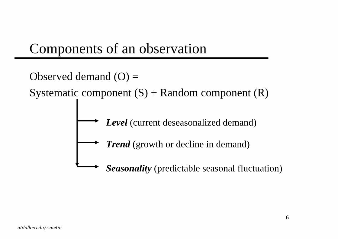
Components of an observation

Observed demand (O) =

Systematic component (S) + Random component (R)

Level (current deseasonalized demand)

Trend (growth or decline in demand)

Seasonality (predictable seasonal fluctuation)

7

utdallas.edu/~metin

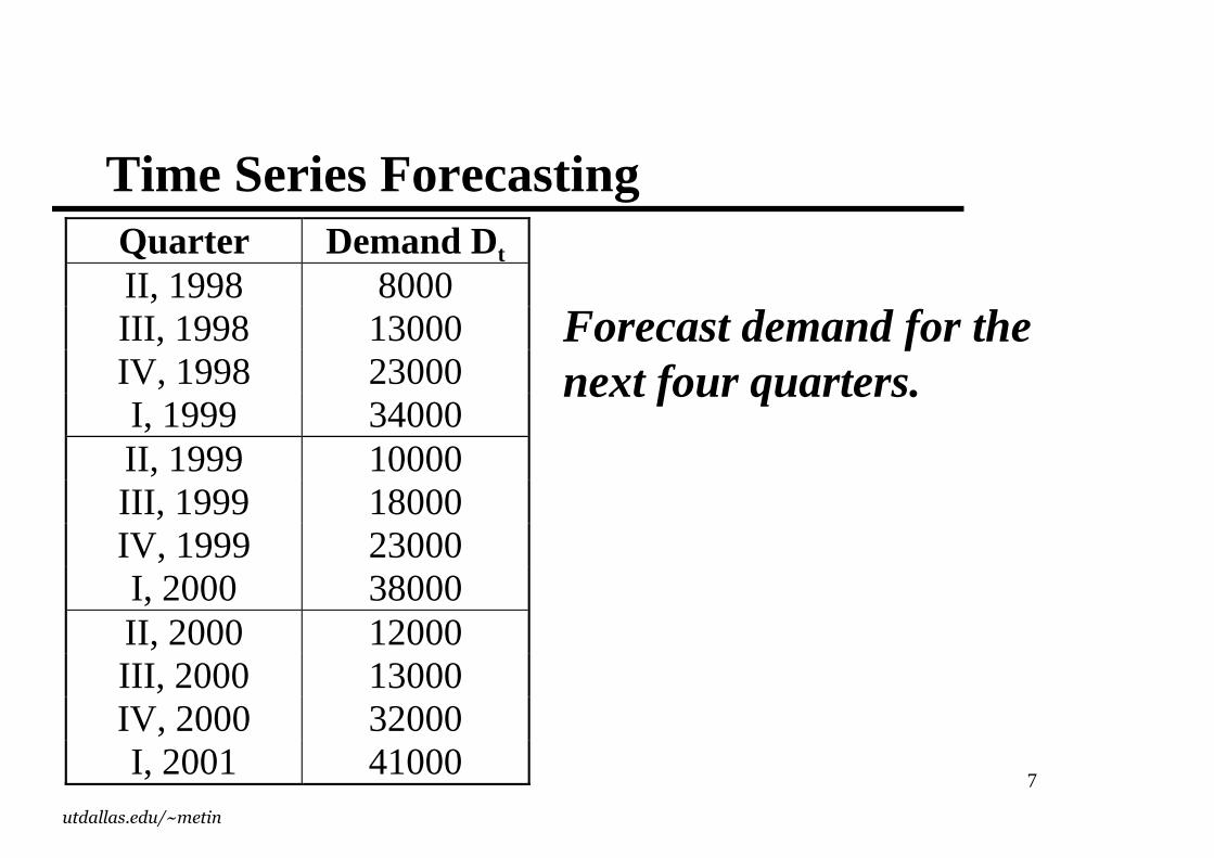
Time Series ForecastingQuarter Demand Dt

II, 1998 8000III, 1998 13000IV, 1998 23000I, 1999 34000II, 1999 10000III, 1999 18000IV, 1999 23000I, 2000 38000II, 2000 12000III, 2000 13000IV, 2000 32000I, 2001 41000

Forecast demand for thenext four quarters.

8

utdallas.edu/~metin

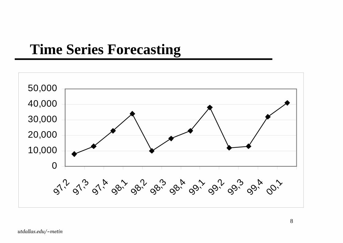
Time Series Forecasting

0

10,000

20,000

30,000

40,000

50,000

97,2

97,3

97,4

98,1

98,2

98,3

98,4

99,1

99,2

99,3

99,4

00,1

9

utdallas.edu/~metin

Forecasting methods

� Static

� Adaptive– Moving average

– Simple exponential smoothing

– Holt’s model (with trend)

– Winter’s model (with trend and seasonality)

10

utdallas.edu/~metin

Error measures

�MAD

�Mean Squared Error (MSE)

�Mean Absolute Percentage Error (MAPE)

� Bias

� Tracking Signal

11

utdallas.edu/~metin

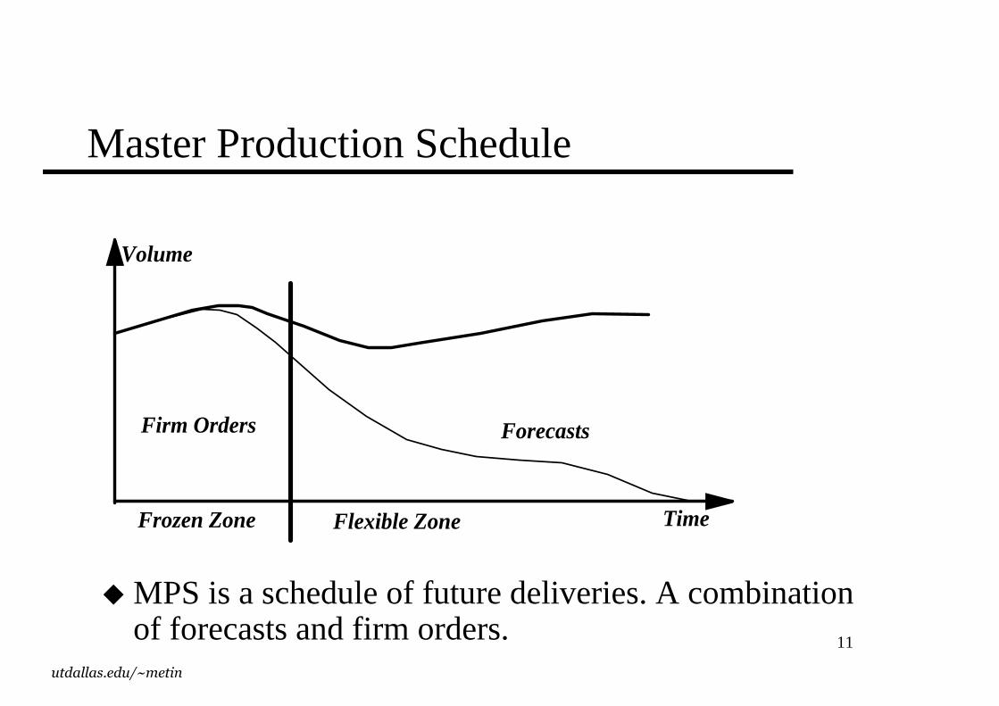
Master Production Schedule

�MPS is a schedule of future deliveries. A combination of forecasts and firm orders.

Volume

Time

Firm Orders Forecasts

Frozen Zone Flexible Zone

12

utdallas.edu/~metin

Aggregate Planning

� If actual is different than plan, why bother sweating over detailed plans� Aggregate planning: General plan

– Combined products = aggregate product» Short and long sleeve shirts = shirt � Single product

– Pooled capacities = aggregated capacity» Dedicated machine and general machine = machine� Single capacity

– Time periods = time buckets» Consider all the demand and production of a given month together� Quite a few time buckets � When does the demand or production take place in a time bucket?

13

utdallas.edu/~metin

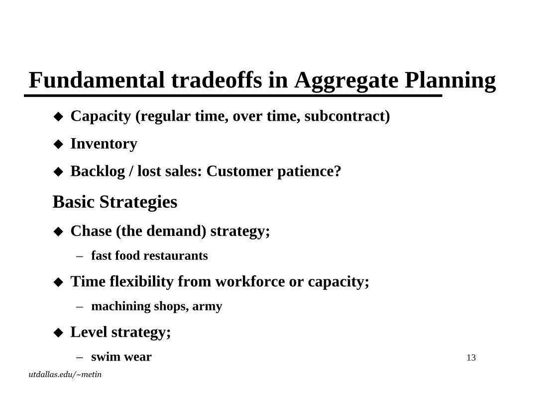
Fundamental tradeoffs in Aggregate Planning� Capacity (regular time, over time, subcontract)

� Inventory

� Backlog / lost sales: Customer patience?

Basic Strategies

� Chase (the demand) strategy;

– fast food restaurants

� Time flexibility from workforce or capacity;

– machining shops, army

� Level strategy;

– swim wear

14

utdallas.edu/~metin

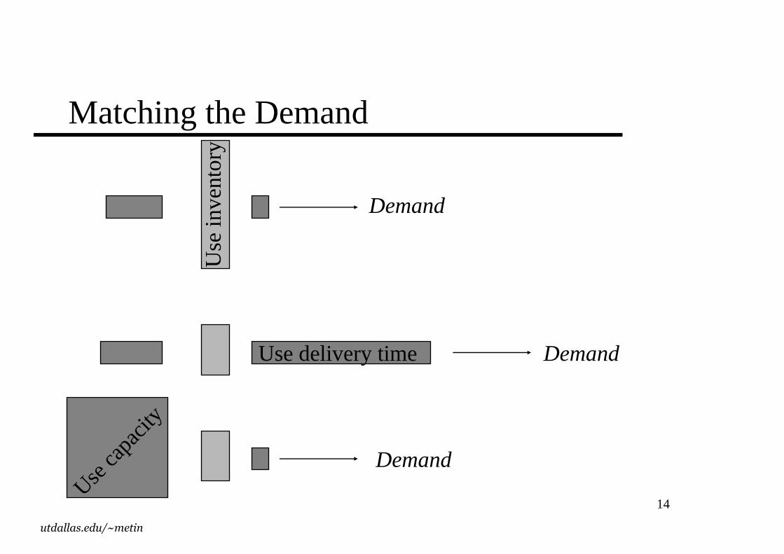
Matching the Demand

Use

inve

ntor

y

Use delivery time

Use ca

pacit

y

Demand

Demand

Demand

15

utdallas.edu/~metin

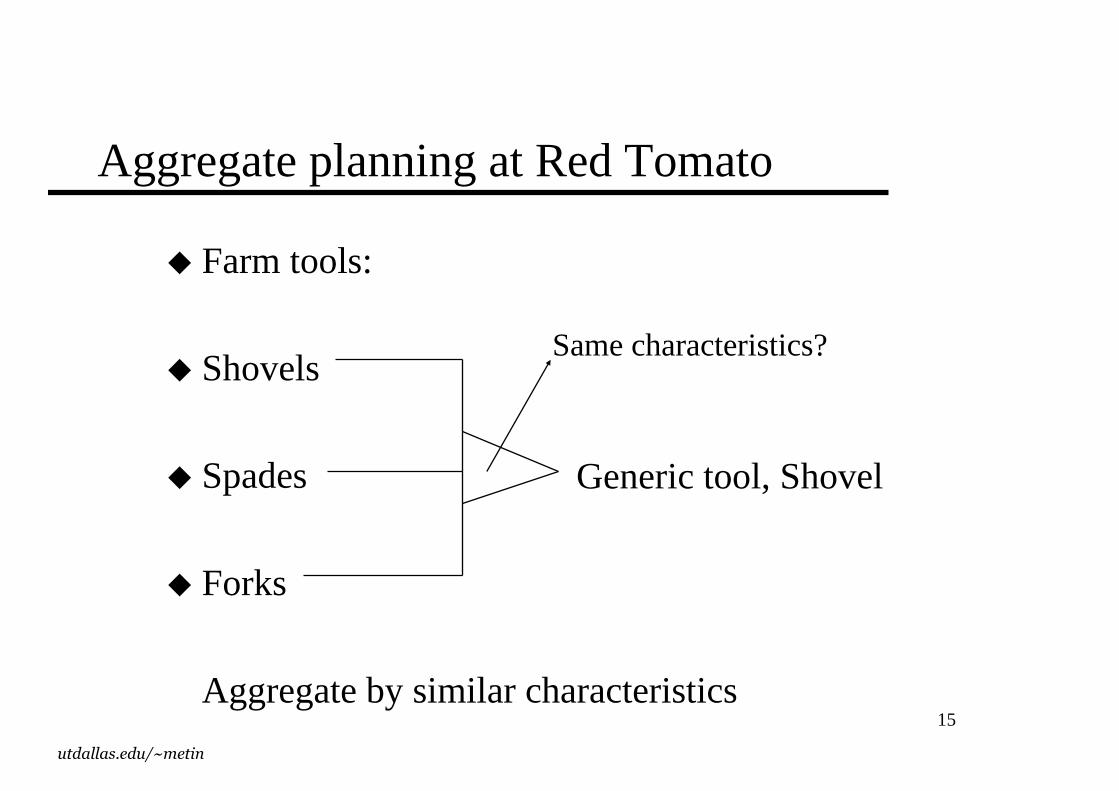
Aggregate planning at Red Tomato

� Farm tools:

� Shovels

� Spades

� Forks

Aggregate by similar characteristics

Generic tool, Shovel

Same characteristics?

16

utdallas.edu/~metin

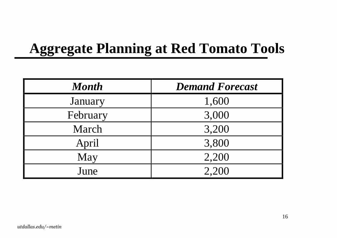
Aggregate Planning at Red Tomato Tools

Month Demand ForecastJanuary 1,600February 3,000March 3,200April 3,800May 2,200June 2,200

17

utdallas.edu/~metin

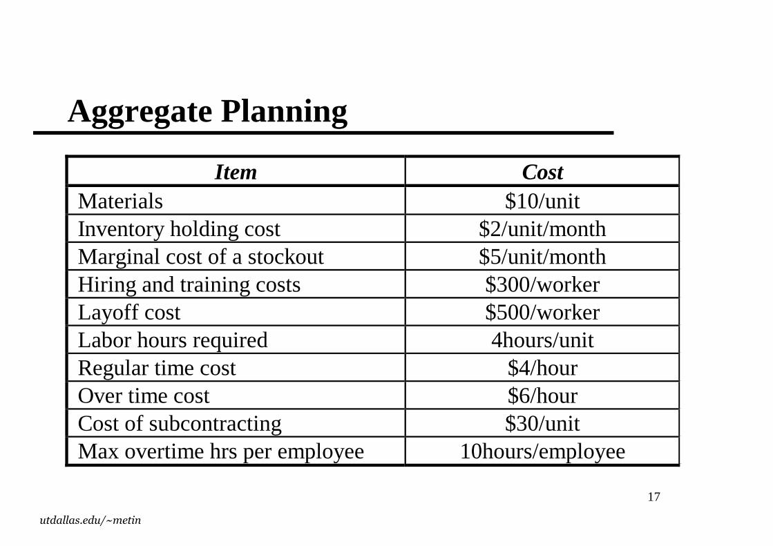
Aggregate Planning

Item Cost Materials $10/unit Inventory holding cost $2/unit/month Marginal cost of a stockout $5/unit/month Hiring and training costs $300/worker Layoff cost $500/worker Labor hours required 4hours/unit Regular time cost $4/hour Over time cost $6/hour Cost of subcontracting $30/unit Max overtime hrs per employee 10hours/employee

18

utdallas.edu/~metin

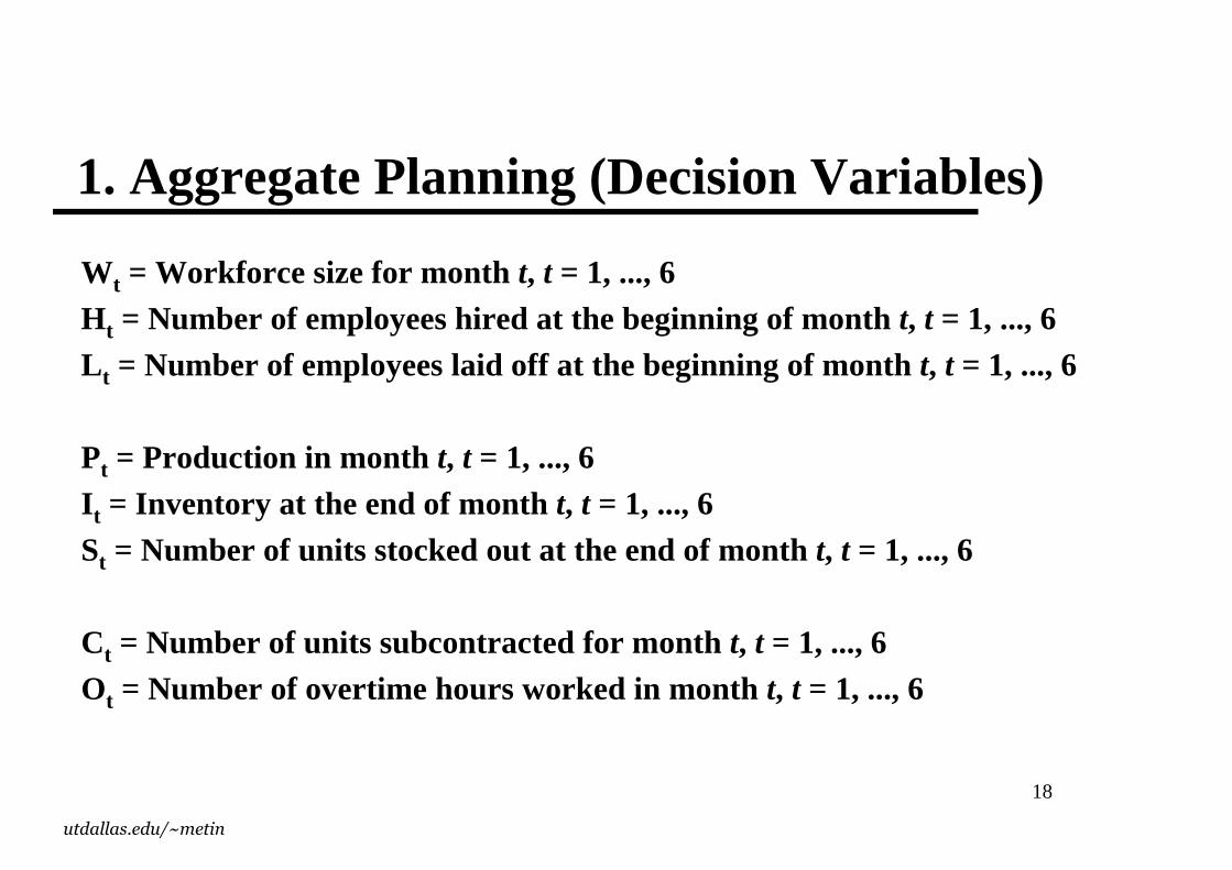
1. Aggregate Planning (Decision Variables)

Wt = Workforce size for month t, t = 1, ..., 6Ht = Number of employees hired at the beginning of month t, t = 1, ..., 6

Lt = Number of employees laid off at the beginning of month t, t = 1, ..., 6

Pt = Production in month t, t = 1, ..., 6It = Inventory at the end of month t, t = 1, ..., 6

St = Number of units stocked out at the end of month t, t = 1, ..., 6

Ct = Number of units subcontracted for month t, t = 1, ..., 6Ot = Number of overtime hours worked in month t, t = 1, ..., 6

19

utdallas.edu/~metin

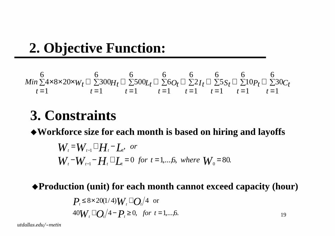
2. Objective Function:

.80 ,6,...,1 0

,

01

1

===+−−

−+=

−

−

WLHWWLHWW

wheretfor

or

tttt

tttt

∑=

+∑=

+∑=

+∑=

+∑=

+∑=

+∑=

+∑=

×××6

130

6

110

6

15

6

12

6

16

6

1500

6

1300

6

12084

tCt

tPt

tSt

tIt

tOt

tLt

tHt

tWtMin

3. Constraints�Workforce size for each month is based on hiring and layoffs

�Production (unit) for each month cannot exceed capacity (hour)

.6,...,1 ,0440

or 4)4/1(208

=≥−+

+×≤

tforPOWOWP

ttt

ttt

20

utdallas.edu/~metin

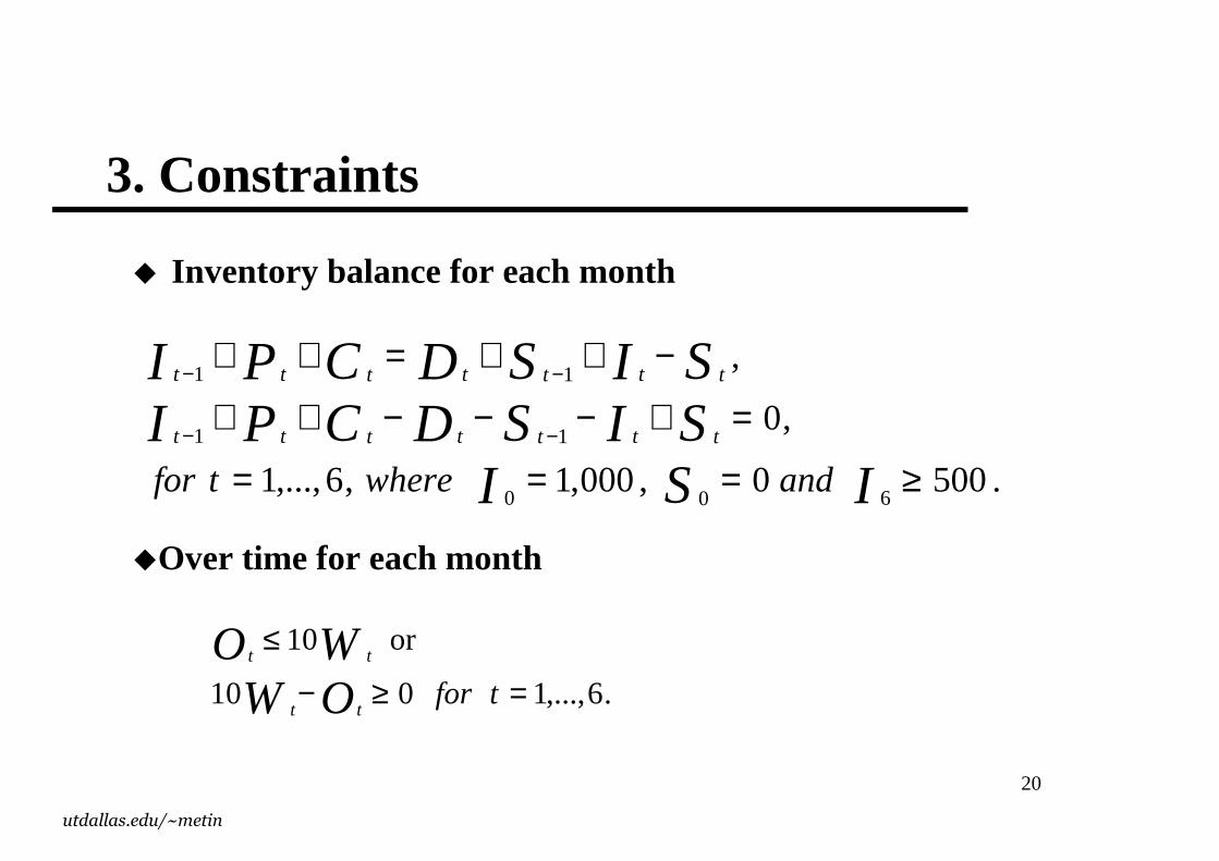
3. Constraints

� Inventory balance for each month

.500 0,000,1 ,6,...,1

,0

,

600

11

11

≥===

=+−−−++

−++=++

−−

−−

ISISISDCPISISDCPI

andwheretforttttttt

ttttttt

�Over time for each month

.6,...,1 010

or 10

=≥−

≤

tforOWWO

tt

tt

21

utdallas.edu/~metin

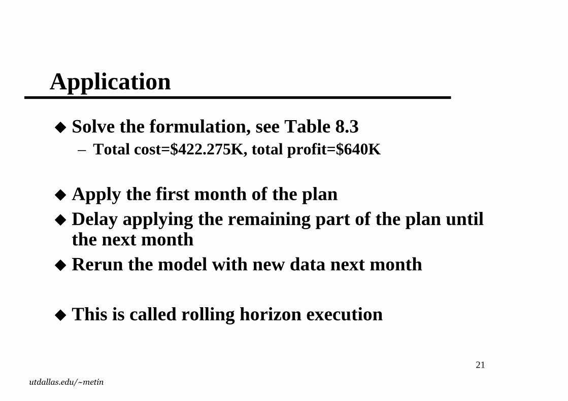
Application

� Solve the formulation, see Table 8.3– Total cost=$422.275K, total profit=$640K

� Apply the first month of the plan � Delay applying the remaining part of the plan until

the next month� Rerun the model with new data next month

� This is called rolling horizon execution

22

utdallas.edu/~metin

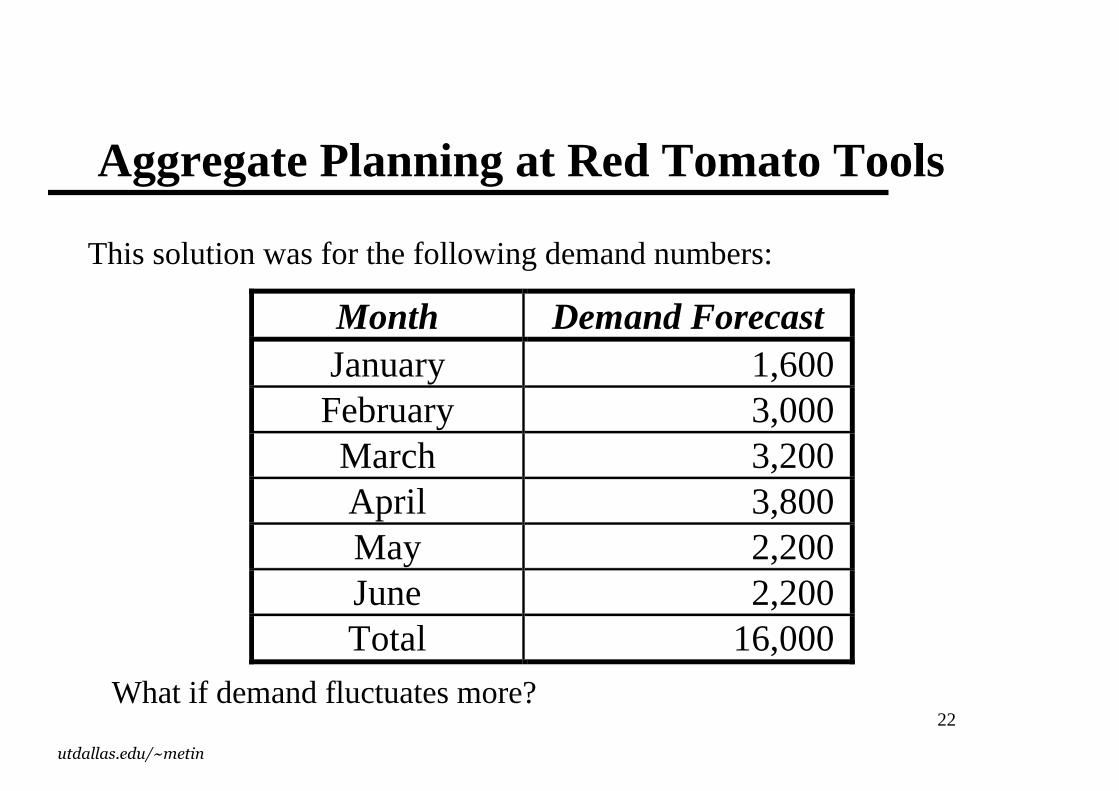
Aggregate Planning at Red Tomato Tools

Month Demand Forecast January 1,600 February 3,000 March 3,200 April 3,800 May 2,200 June 2,200 Total 16,000

This solution was for the following demand numbers:

What if demand fluctuates more?

23

utdallas.edu/~metin

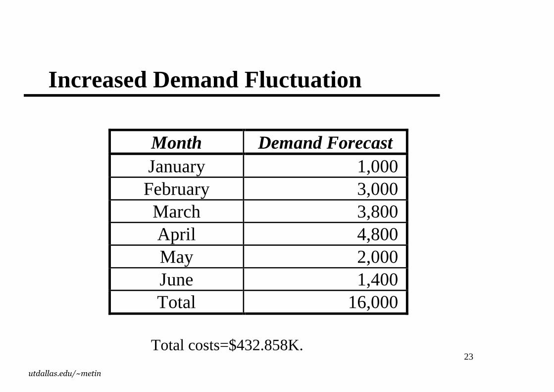
Increased Demand Fluctuation

Month Demand Forecast January 1,000 February 3,000 March 3,800 April 4,800 May 2,000 June 1,400 Total 16,000

Total costs=$432.858K.

24

utdallas.edu/~metin

Chapter 9:Matching Demand and Supply

� Supply = Demand

� Supply < Demand => Lost revenue opportunity

� Supply > Demand => Inventory

�Manage Supply – Productions Management

�Manage Demand – Marketing

25

utdallas.edu/~metin

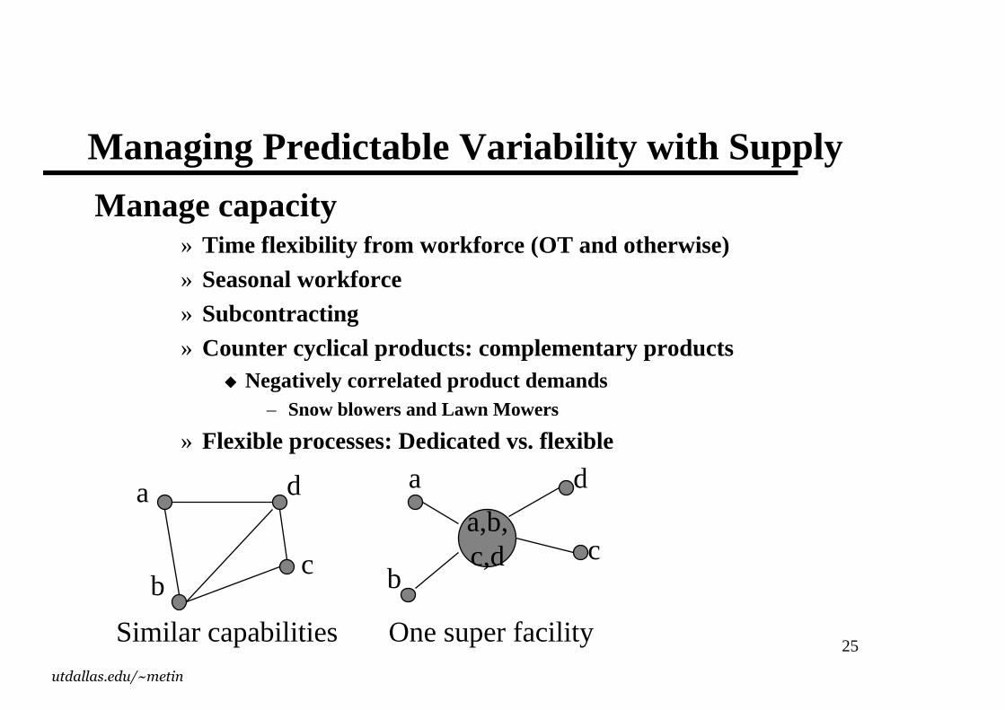
Managing Predictable Variability with Supply

Manage capacity» Time flexibility from workforce (OT and otherwise)» Seasonal workforce» Subcontracting» Counter cyclical products: complementary products� Negatively correlated product demands

– Snow blowers and Lawn Mowers

» Flexible processes: Dedicated vs. flexible

a,b,c,d

Similar capabilities One super facility

a

bc

d a

bc

d

26

utdallas.edu/~metin

Managing Predictable Variability with Inventory

» Component commonality� Remember fast food restaurant menus

» Build seasonal inventory of predictable products in preseason� Nothing can be learnt by procrastinating

» Keep inventory of predictable products in the downstream supply chain

27

utdallas.edu/~metin

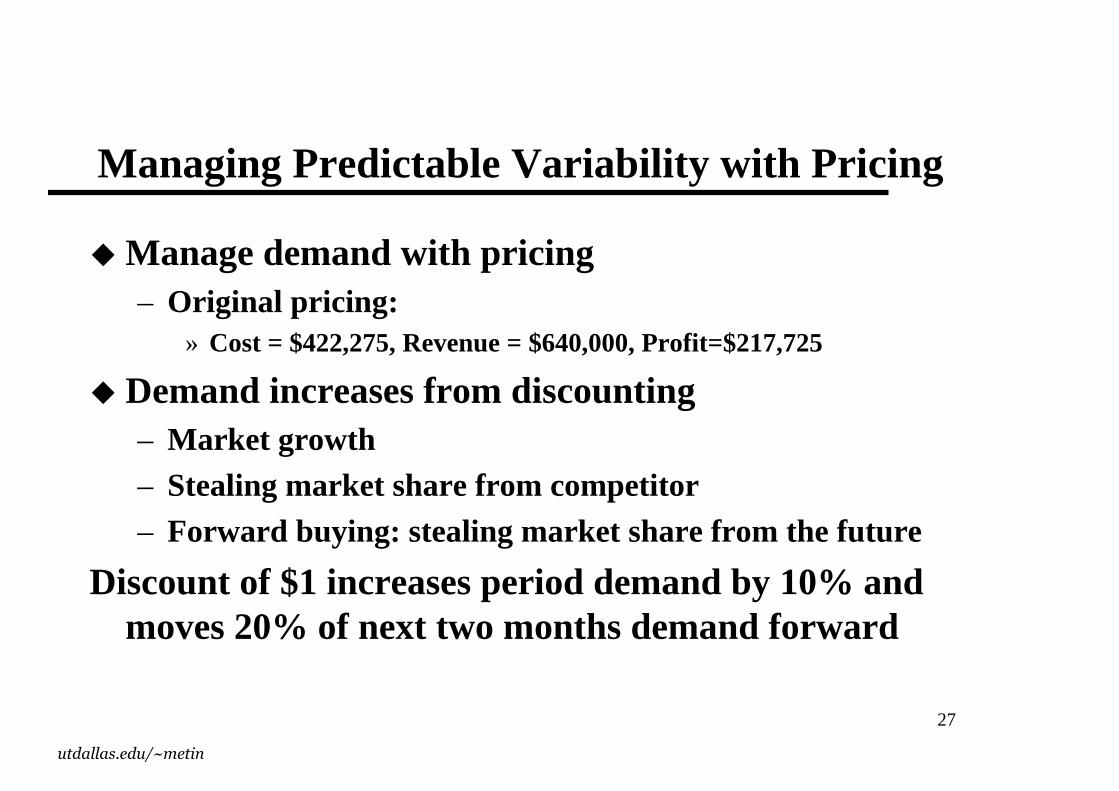
Managing Predictable Variability with Pricing

�Manage demand with pricing– Original pricing:

» Cost = $422,275, Revenue = $640,000, Profit=$217,725

� Demand increases from discounting– Market growth– Stealing market share from competitor– Forward buying: stealing market share from the future

Discount of $1 increases period demand by 10% and moves 20% of next two months demand forward

28

utdallas.edu/~metin

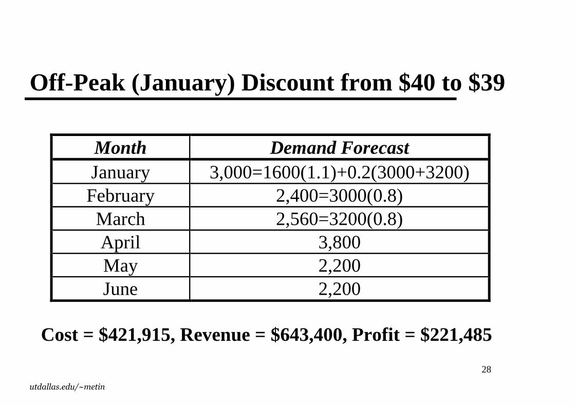
Off-Peak (January) Discount from $40 to $39

Month Demand Forecast January 3,000=1600(1.1)+0.2(3000+3200) February 2,400=3000(0.8) March 2,560=3200(0.8) April 3,800 May 2,200 June 2,200

Cost = $421,915, Revenue = $643,400, Profit = $221,485

29

utdallas.edu/~metin

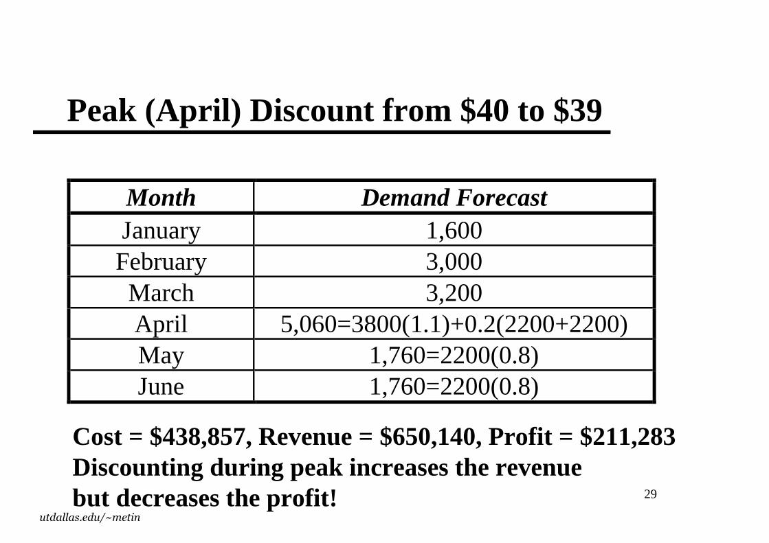
Peak (April) Discount from $40 to $39

Month Demand Forecast January 1,600 February 3,000 March 3,200 April 5,060=3800(1.1)+0.2(2200+2200) May 1,760=2200(0.8) June 1,760=2200(0.8)

Cost = $438,857, Revenue = $650,140, Profit = $211,283Discounting during peak increases the revenue but decreases the profit!

30

utdallas.edu/~metin

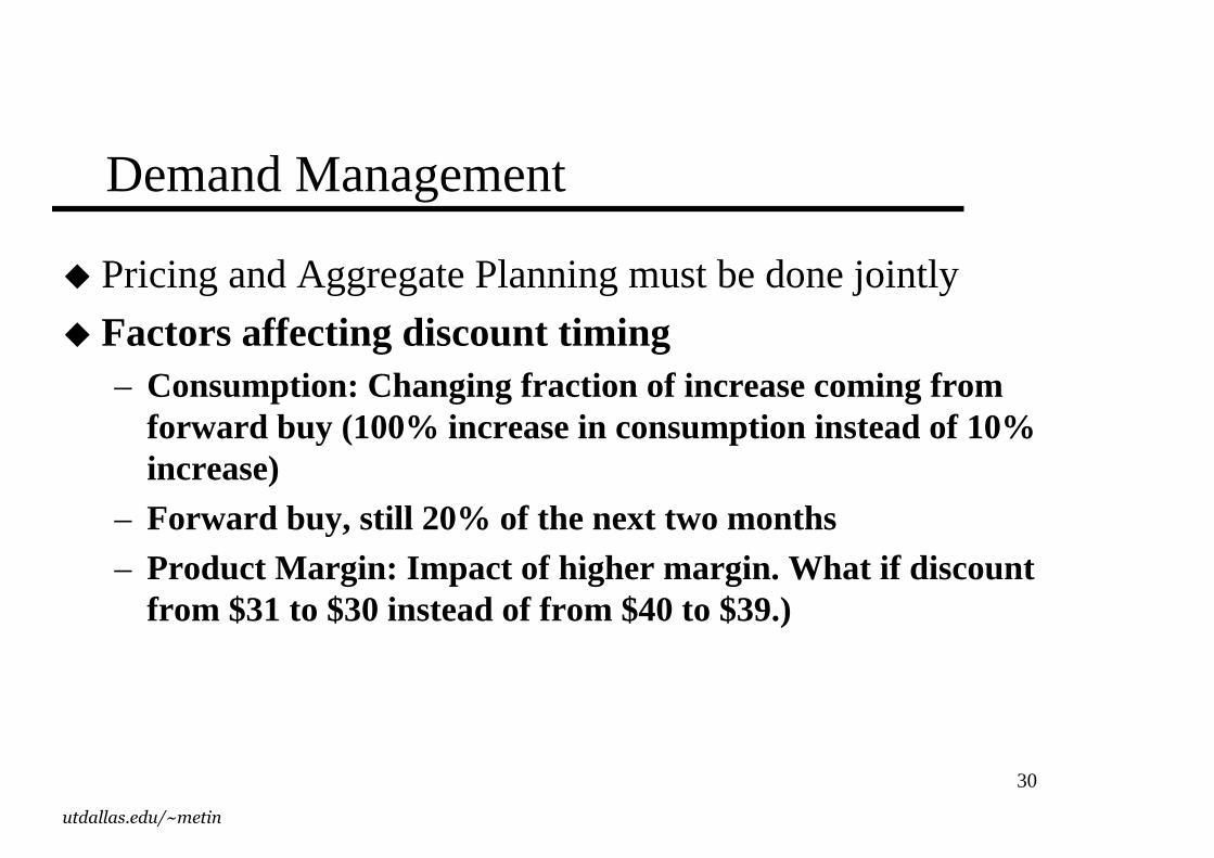
Demand Management

� Pricing and Aggregate Planning must be done jointly

� Factors affecting discount timing– Consumption: Changing fraction of increase coming from

forward buy (100% increase in consumption instead of 10% increase)

– Forward buy, still 20% of the next two months– Product Margin: Impact of higher margin. What if discount

from $31 to $30 instead of from $40 to $39.)

31

utdallas.edu/~metin

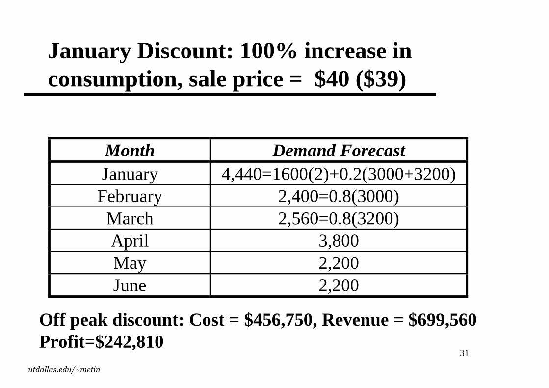
January Discount: 100% increase in consumption, sale price = $40 ($39)

Month Demand Forecast January 4,440=1600(2)+0.2(3000+3200) February 2,400=0.8(3000) March 2,560=0.8(3200) April 3,800 May 2,200 June 2,200

Off peak discount: Cost = $456,750, Revenue = $699,560Profit=$242,810

32

utdallas.edu/~metin

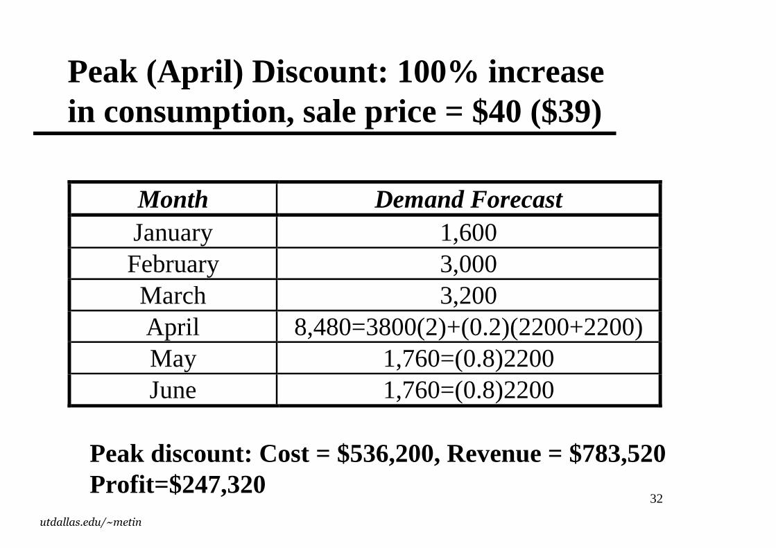
Peak (April) Discount: 100% increase in consumption, sale price = $40 ($39)

Month Demand Forecast January 1,600 February 3,000 March 3,200 April 8,480=3800(2)+(0.2)(2200+2200) May 1,760=(0.8)2200 June 1,760=(0.8)2200

Peak discount: Cost = $536,200, Revenue = $783,520Profit=$247,320

33

utdallas.edu/~metin

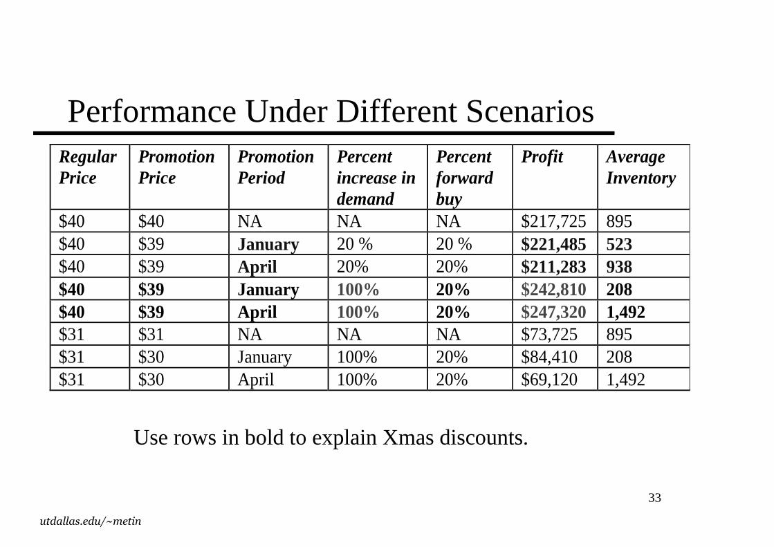
Performance Under Different ScenariosRegular Price

Promotion Price

Promotion Period

Percent increase in demand

Percent forward buy

Profit Average Inventory

$40 $40 NA NA NA $217,725 895 $40 $39 January 20 % 20 % $221,485 523 $40 $39 April 20% 20% $211,283 938 $40 $39 January 100% 20% $242,810 208 $40 $39 April 100% 20% $247,320 1,492 $31 $31 NA NA NA $73,725 895 $31 $30 January 100% 20% $84,410 208 $31 $30 April 100% 20% $69,120 1,492

Use rows in bold to explain Xmas discounts.

34

utdallas.edu/~metin

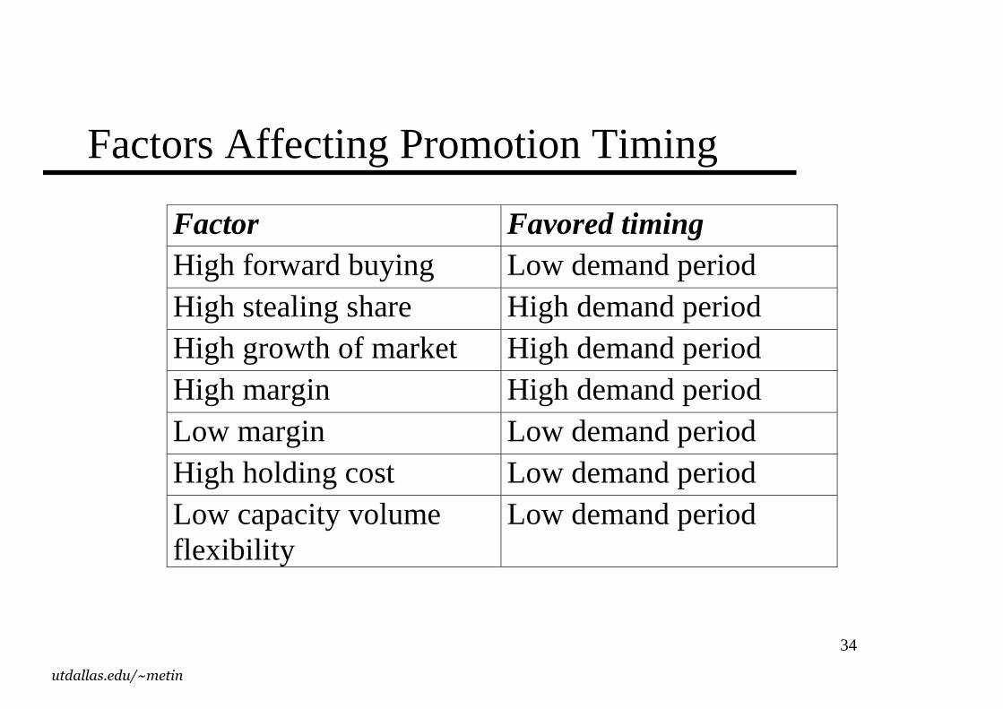
Factors Affecting Promotion Timing

Factor Favored timing High forward buying Low demand period High stealing share High demand period High growth of market High demand period High margin High demand period Low margin Low demand period High holding cost Low demand period Low capacity volume flexibility

Low demand period

35

utdallas.edu/~metin

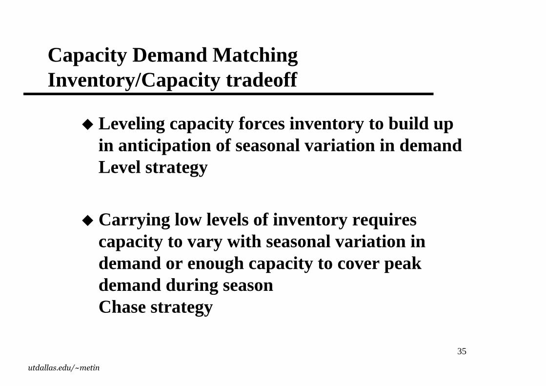
Capacity Demand MatchingInventory/Capacity tradeoff

� Leveling capacity forces inventory to build up in anticipation of seasonal variation in demand Level strategy

� Carrying low levels of inventory requires capacity to vary with seasonal variation in demand or enough capacity to cover peak demand during season Chase strategy

36

utdallas.edu/~metin

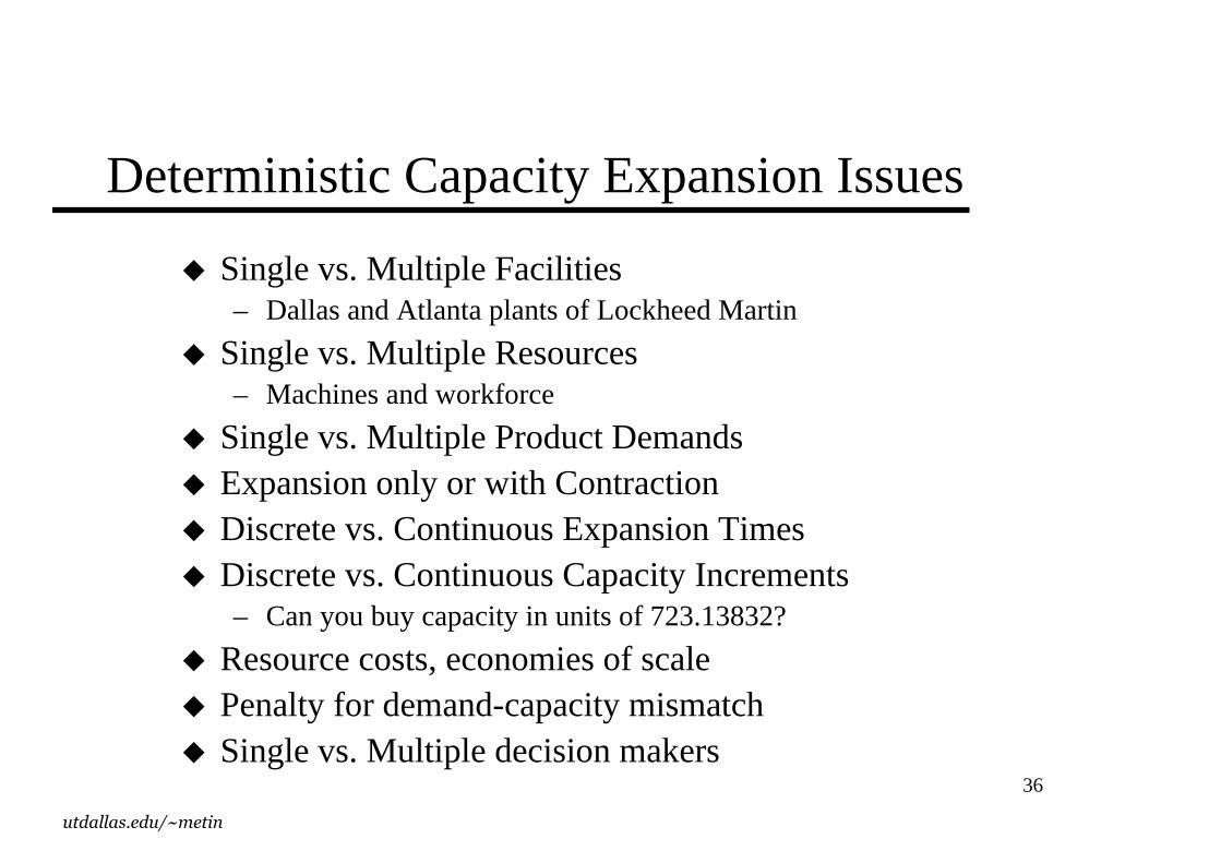
Deterministic Capacity Expansion Issues

� Single vs. Multiple Facilities– Dallas and Atlanta plants of Lockheed Martin

� Single vs. Multiple Resources– Machines and workforce

� Single vs. Multiple Product Demands� Expansion only or with Contraction� Discrete vs. Continuous Expansion Times� Discrete vs. Continuous Capacity Increments

– Can you buy capacity in units of 723.13832?

� Resource costs, economies of scale� Penalty for demand-capacity mismatch� Single vs. Multiple decision makers

37

utdallas.edu/~metin

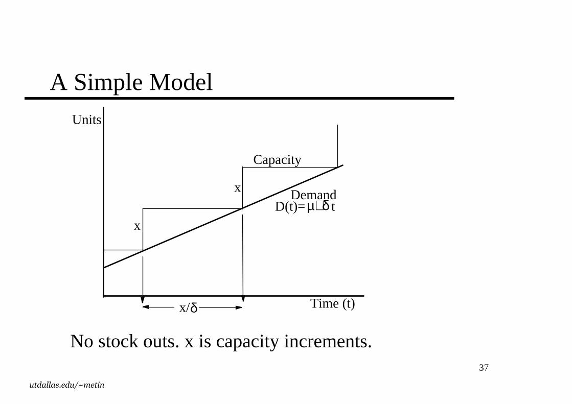
A Simple Model

No stock outs. x is capacity increments.

D(t)=µ+δ t

x

Demand

Capacity

Units

Time (t)x/δ

x

38

utdallas.edu/~metin

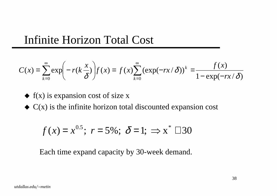
Infinite Horizon Total Cost

� f(x) is expansion cost of size x

� C(x) is the infinite horizon total discounted expansion cost

)/exp(1

)())/(exp()()()(exp)(

00 δδ

δ rx

xfrxxfxf

xkrxC

k

k

k −−=−=

−= ∑∑ ∞

=

∞

=

30 x ;1 %;5 ;)( *5.0 ≅⇒=== δrxxf

Each time expand capacity by 30-week demand.

39

utdallas.edu/~metin

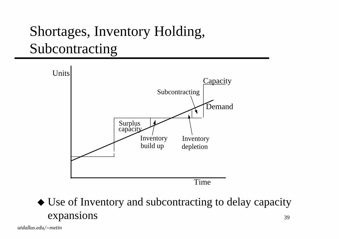
Shortages, Inventory Holding, Subcontracting

� Use of Inventory and subcontracting to delay capacity expansions

Demand

Units

Time

Capacity

Surpluscapacity

Inventorybuild up

Inventorydepletion

Subcontracting

40

utdallas.edu/~metin

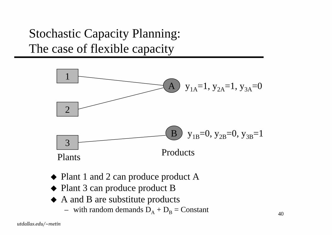
Stochastic Capacity Planning: The case of flexible capacity

� Plant 1 and 2 can produce product A� Plant 3 can produce product B� A and B are substitute products

– with random demands DA + DB = Constant

1

2

3

A

B

Plants Products

y1A=1, y2A=1, y3A=0

y1B=0, y2B=0, y3B=1

41

utdallas.edu/~metin

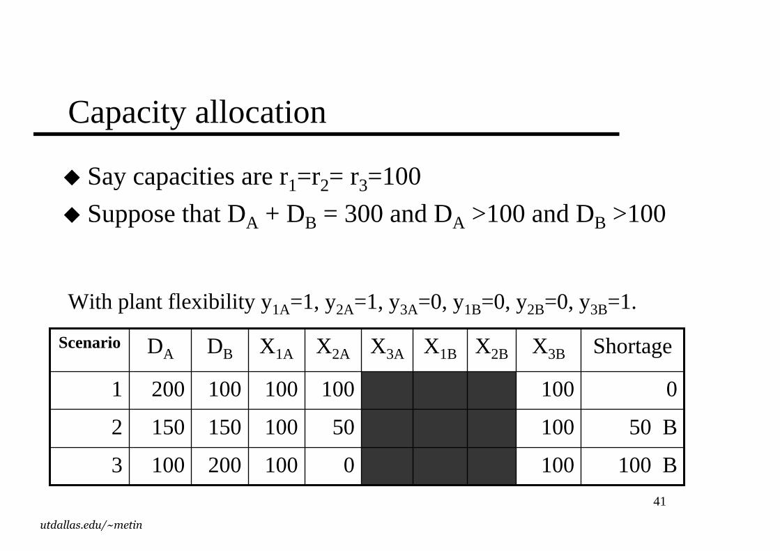
Capacity allocation

� Say capacities are r1=r2= r3=100

� Suppose that DA + DB = 300 and DA >100 and DB >100

100 B

50 B

0

Shortage

3

2

1

Scenario

1000100200100

10050100150150

100100100100200

X3BX2BX1BX3AX2AX1ADBDA

With plant flexibility y1A=1, y2A=1, y3A=0, y1B=0, y2B=0, y3B=1.

42

utdallas.edu/~metin

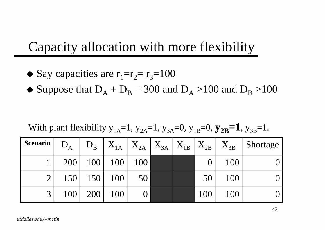
Capacity allocation with more flexibility

� Say capacities are r1=r2= r3=100

� Suppose that DA + DB = 300 and DA >100 and DB >100

0

0

0

Shortage

3

2

1

Scenario

1001000100200100

1005050100150150

1000100100100200

X3BX2BX1BX3AX2AX1ADBDA

With plant flexibility y1A=1, y2A=1, y3A=0, y1B=0, y2B=1, y3B=1.

43

utdallas.edu/~metin

Material Requirements Planning

�Master Production Schedule (MPS)� Bill of Materials (BOM)�MRP explosion� Advantages

– Disciplined database– Component commonality

� Shortcomings– Rigid lead times– No capacity consideration

44

utdallas.edu/~metin

Optimized Production Technology

� Focus on bottleneck resources to simplify planning

� Product mix defines the bottleneck(s) ?

� Provide plenty of non-bottleneck resources.

� Shifting bottlenecks

45

utdallas.edu/~metin

Just in Time production

� Focus on timing

� Advocates pull system, use Kanban

� Design improvements encouraged

� Lower inventories / set up time / cycle time

� Quality improvements

� Supplier relations, fewer closer suppliers, Toyota city

� JIT philosophically different than OPT or MRP, it is not only a planning tool but a continuous improvement scheme

46

utdallas.edu/~metin

Summary of Learning Objectives

� Forecasting� Aggregate planning� Supply and demand management during

aggregate planning with predictable demand variation– Supply management levers– Demand management levers

�MRP, OPT, JIT� Deterministic Capacity Planning