Exploring the potential of microwave diagnostics in SEP ... · 1 Exploring the potential of...
23
submitted to Journal of Space Weather and Space Climate c The author(s) under the Creative Commons Attribution-NonCommercial license Exploring the potential of microwave diagnostics 1 in SEP forecasting: 2 The occurrence of SEP events 3 Pietro Zucca 1 , Marlon Nu ˜ nez 2 , and Karl-Ludwig Klein 1 4 1 LESIA-UMR 8109 - Observatoire de Paris, PSL Res. Univ., CNRS, Univ. P & M Curie and 5 Paris-Diderot, 92190 Meudon, France 6 e-mail: [email protected] e-mail: [email protected] 7 8 2 Universidad de Malaga, Malaga, Spain 9 e-mail: [email protected] 10 ABSTRACT 11 Solar energetic particles (SEPs), especially protons and heavy ions, may be a space weather hazard 12 when they impact spacecraft and the terrestrial atmosphere. Forecasting schemes have been devel- 13 oped, which use earlier signatures of particle acceleration to predict the arrival of solar protons and 14 ions in the space environment of the Earth. The UMASEP scheme forecasts the occurrence and 15 the importance of an SEP event based on combined observations of soft X-rays, their time deriva- 16 tive, and protons above 10 MeV at geosynchronous orbit. We explore the possibility to replace the 17 derivative of the soft X-ray time history with the microwave time history in the UMASEP scheme. 18 To this end we construct a continuous time series of observations for a thirteen months period from 19 December 2011 to December 2012 at two microwave frequencies, 4.995 and 8.8 GHz, using data 20 from the four Radio Solar Telescope Network (RSTN) patrol stations of the US Air Force, and feed 21 this time series to the UMASEP prediction scheme. During the selected period the Geostationary 22 Operational Environmental Satellites (GOES) detected nine SEP events related with activity in the 23 western solar hemisphere. We show that the SEP forecasting using microwaves has the same prob- 24 ability of detection as the method using soft X-rays, but no false alarm in the considered period, 25 and a slightly increased warning time. A detailed analysis of the missed events is presented. We 26 conclude that microwave patrol observations improve SEP forecasting schemes that employ soft 27 X-rays. High-quality microwave data available in real time appear as a significant addition to our 28 ability to predict SEP occurrence. 29 Key words. Sun: particle emission; Sun: radio radiation; solar-terrestrial relations 1
Transcript of Exploring the potential of microwave diagnostics in SEP ... · 1 Exploring the potential of...

submitted to Journal of Space Weather and Space Climatec© The author(s) under the Creative Commons Attribution-NonCommercial license
Exploring the potential of microwave diagnostics1
in SEP forecasting:2
The occurrence of SEP events3
Pietro Zucca1, Marlon Nunez2, and Karl-Ludwig Klein14
1 LESIA-UMR 8109 - Observatoire de Paris, PSL Res. Univ., CNRS, Univ. P & M Curie and5
Paris-Diderot, 92190 Meudon, France6
e-mail: [email protected] e-mail: [email protected]
8
2 Universidad de Malaga, Malaga, Spain9
e-mail: [email protected]
ABSTRACT11
Solar energetic particles (SEPs), especially protons and heavy ions, may be a space weather hazard12
when they impact spacecraft and the terrestrial atmosphere. Forecasting schemes have been devel-13
oped, which use earlier signatures of particle acceleration to predict the arrival of solar protons and14
ions in the space environment of the Earth. The UMASEP scheme forecasts the occurrence and15
the importance of an SEP event based on combined observations of soft X-rays, their time deriva-16
tive, and protons above 10 MeV at geosynchronous orbit. We explore the possibility to replace the17
derivative of the soft X-ray time history with the microwave time history in the UMASEP scheme.18
To this end we construct a continuous time series of observations for a thirteen months period from19
December 2011 to December 2012 at two microwave frequencies, 4.995 and 8.8 GHz, using data20
from the four Radio Solar Telescope Network (RSTN) patrol stations of the US Air Force, and feed21
this time series to the UMASEP prediction scheme. During the selected period the Geostationary22
Operational Environmental Satellites (GOES) detected nine SEP events related with activity in the23
western solar hemisphere. We show that the SEP forecasting using microwaves has the same prob-24
ability of detection as the method using soft X-rays, but no false alarm in the considered period,25
and a slightly increased warning time. A detailed analysis of the missed events is presented. We26
conclude that microwave patrol observations improve SEP forecasting schemes that employ soft27
X-rays. High-quality microwave data available in real time appear as a significant addition to our28
ability to predict SEP occurrence.29
Key words. Sun: particle emission; Sun: radio radiation; solar-terrestrial relations
1
Zucca et al.: Accepted for publication in the Journal of SWSC.
1. Introduction30
Solar energetic particles (SEPs), especially protons and heavy ions, can disturb or damage electronic31
equipment aboard spacecraft, affect the ionization and chemistry of the high terrestrial atmosphere,32
and create secondaries that interact with equipment and living beings aboard aircraft. SEPs may33
be a major space weather hazard, and a fundamental concern to manned spaceflight. Forecasting34
the occurrence and importance of an SEP event is therefore a task for space weather research, and35
appears mandatory if human beings are to be sent aboard spacecraft beyond low-Earth orbit. SEPs36
are accelerated in relationship with major eruptive events in the corona, flares and coronal mass37
ejections (CMEs).38
As of today, it is not possible to reliably predict a flare or a CME. It is also not possible to predict39
before the eruptive event whether it will lead to a major SEP event or not. The only practicable40
forecasting strategy is presently to infer the SEPs to come from the first observations of the eruptive41
activity in the corona or from early signatures of fast particles themselves. Several different, but42
complementary approaches have been developed. Some use the analysis of solar electromagnetic43
radiation as the basic ingredient. Because of their continuous availability, soft X-ray observations44
by the Geostationary Orbiting Environmental Satellites (GOES) of NOAA play a key role in these45
forecasting schemes.46
The empirical forecast systems of the US Air Force (Smart and Shea, 1992; Kahler et al., 2007)47
and of the NOAA Space Weather Prediction Center (Balch, 2008) are based on the location of the48
flare and the importance and time evolution of the associated soft X-ray burst. The USAF system49
predicts the onset, rise time and peak of the SEP event at several energies above 5 MeV, radiation50
dose rates in the terrestrial atmosphere and ionospheric absorption. The NOAA system uses in ad-51
dition the occurrence of metre-wave radio emission related to CMEs and shocks. It predicts the52
probability of occurrence of an SEP event, the maximum intensity and its time. Both schemes are53
semi-automatic, in that operators are supposed to use them for a final decision on whether an event54
is to be predicted or not. Laurenza et al. (2009) added an observational criterion of the escape of par-55
ticles accelerated in the corona to the interplanetary space, using the observation of decametric-to-56
kilometric radio emission from electron beams that travel through the high corona (type III bursts).57
Garcia (2004), Belov (2009) and the COMESEP model (Dierckxsens et al., 2015) propose methods58
that calculate the probability of SEP events from X-ray observations. The empirical and operational59
SEP forecasting methods using electromagnetic observations of solar activity currently rely more60
on data related to the flare rather than the CME-driven shock to predict well-connected SEP events.61
Physics-based SEP forecasting models have so far been mostly developed based on shock accel-62
eration theories or on particle transport modelling, assuming injections into the interplanetary space63
from an unspecified generic accelerator. These models are not operational yet. Physics-based par-64
ticle models like SOLPENCO1 (Aran et al., 2006, 2008) and SPARX Marsh et al. (2015) are able65
to make a post-event prediction of the SEP intensity profiles. The core of SOLPENCO contains a66
database of pre-calculated synthetic flux profiles of gradual proton events for different interplane-67
tary scenarios for energies up to 200 MeV. SPARX uses a pre-generated database of model runs68
containing varying proton injection locations for energies in the ranges E>10 MeV and E>60 MeV.69
1 http://dev.sepem.oma.be/help/solpenco2_intro.html
2

Zucca et al.: Accepted for publication in the Journal of SWSC.
When SEP forecasting is based exclusively on solar radiative signatures, there is no certainty70
whether the Earth or the spacecraft of interest are magnetically connected to the particle accelerator71
or not. The location of the eruptive activity is only a partial indicator. The problem is avoided by72
forecasting schemes based on in situ observations of energetic particles themselves. The longest73
warning times are achieved when the particles employed are particularly fast. The RELEASE sys-74
tem (Posner, 2007) uses energetic electrons, while the GLE-Alert system (Souvatzoglou et al., 2014)75
is based on relativistic protons observed by neutron monitors.76
The UMASEP scheme (Nunez, 2011) combines the monitoring of solar soft X-ray emission,77
its time-derivative and solar protons, using GOES measurements. Simultaneous rises in the soft78
X-ray flux and the particle intensity are considered as an indicator that an SEP event is to occur.79
We conduct an exploratory study to see if the soft X-ray data can be replaced or complemented by80
microwave observations referring to the gyrosynchrotron emission of mildly relativistic electrons81
accelerated in the associated flare. The motivation is twofold: from a physics viewpoint microwave82
emission produced by non-thermal electrons may be expected to be more closely related to SEP83
acceleration than soft X-rays, which are emitted by the plasma heated during the solar eruption.84
From an empirical viewpoint, the derivative of the soft X-ray time profile is known to mimic the85
time profile of microwave emission from non-thermal electrons. The UMASEP scheme and the mi-86
crowave emission are briefly introduced in Section 2. In Section 3 composite profiles of microwave87
flux densities during a 13-months interval are presented, and the results of a run of UMASEP with88
these data are described. The reasons for erroneous predictions are studied in detail in Section 4.89
The usefulness of microwave data is discussed in the light of these results in Section 5.90
2. The UMASEP prediction scheme and microwave burst emission91
2.1. The UMASEP model for well-connected SEP events92
The UMASEP scheme (Nunez, 2011) comprises two different procedures to forecast SEP events,93
which are referred to as “well-connected” and “poorly-connected” prediction models. The predic-94
tion model of “well-connected” events uses the common rise, with a plausible time delay, of the soft95
X-ray flux of the Sun and the intensities of protons in each of the energy channels measured by the96
GOES particle detectors, i.e. 9-500 MeV. The correlated occurrence of the two rises is considered as97
evidence that they are physically related to a common energy release at the Sun. The region of the98
solar energy release and the spacecraft are therefore considered as being magnetically connected,99
and the events are referred to as “well-connected” events.100
In the literature the term “well-connected” is in general employed for solar activity that occurs101
in some restricted range of heliolongitudes around the nominal footpoint at the Sun of the Parker102
spiral through the observing point, the Earth or a spacecraft. Since the Parker spiral is an aver-103
age description of the interplanetary magnetic field, this definition may not be adequate in each104
individual case, notably when the interplanetary magnetic field is perturbed by coronal mass ejec-105
tions (Richardson and Cane, 1996; Masson et al., 2012). In addition, even when the interplanetary106
magnetic field is adequately described by a Parker spiral, energetic particles may have access to a107
given field line from a broad range of heliolongitudes. This is the case on the one hand when the108
acceleration region is broad, for instance an extended shock front (Lee et al., 2012). On the other109
hand the Parker spiral is rooted on the source surface of the solar wind, at some distance from the110
3

Zucca et al.: Accepted for publication in the Journal of SWSC.
photosphere. The open magnetic field lines that connect an active region in the low corona to this111
footpoint may spread apart with increasing altitude and cover an extended range of heliolongitudes112
(Klein et al., 2008). In all these cases SEPs can reach the spacecraft along magnetic field lines from113
longitudes that would be characterised as being poorly-connected if the definition referred to the114
nominal Parker spiral. The direct comparison between the rise of particle intensities at a spacecraft115
and a signature of coronal activity gives physical meaning to the term “connection”.116
The UMASEP model for predicting well-connected events, called here WCP model, issues an117
SEP prediction if at least one of the correlations between the proton intensities and the soft X-ray118
flux is high, and if the associated X-ray burst is also strong. This approach has two limitations:119
On the one hand the correlation between the rises of the X-ray emission and the SEP intensity120
must not be coincidental. This is a hypothesis, which is validated by the success of the forecasting121
procedure. On the other hand, the procedure works only when the solar activity is on the visible122
disk. SEP events may be observed at Earth even when the parent activity is behind the solar limb.123
This can be due to the interplanetary transport, which may carry SEPs across magnetic field lines124
(Dresing et al., 2014; Laitinen and Dalla, 2017), or to a direct magnetic connection. However, the125
peak intensity and therefore the space-weather relevance of events that are more than 10 behind the126
west limb or more than 20 east of central meridian decreases significantly, as shown for instance127
in Fig. 12 of Richardson et al. (2014). Within the UMASEP scheme, such events can still be pre-128
dicted by a different approach, called the “poorly connected” (PCP) model, which does not employ129
electromagnetic data. For this reason we do not consider this model any more in the following. The130
term “poorly connected” is misleading in those cases where parent activity behind the limb has a131
magnetic connection to the terrestrial observer. This has to be kept in mind when employing the132
conventional UMASEP nomenclature as described above.133
The aforementioned scheme has been used to build several tools: UMASEP-10 (Nunez, 2011),134
the first of these tools, predicts well- and poorly-connected SEP events > 10 MeV from soft X-ray135
and proton fluxes; UMASEP-100 (Nunez, 2015), a tool for predicting well-connected > 100 MeV136
SEP events from soft X-ray and proton data; HESPERIA UMASEP-500 (Nunez et al. 2017, in137
preparation), a tool for predicting well-connected > 500 MeV events from soft X-ray, proton and138
neutron monitor data. HESPERIA UMASEP-10mw, the tool that is introduced in the present paper,139
is devised to predict SEP events with energies > 10 MeV from microwave and proton data. Real-140
time UMASEP-10 forecasts are publicly available since 2010 in NASA’s integrated Space Weather141
Analysis (iSWA) system2, in the European Space Weather Portal3, as well as in the University of142
Malaga’s space weather portal4. UMASEP-10 was also included as a module in the European Space143
Agency’s SEPsFLAREs system (Garcıa-Rigo et al., 2016). Section 2.2 describes the UMASEP144
scheme, and section 2.4 the adaptation of this scheme to build the tool UMASEP-10mw using145
microwave data.146
2 http://iswa.ccmc.gsfc.nasa.gov/IswaSystemWebApp/index.jsp?i_1=141&l_1=40&t_1=
270&w_1=600&h_1=5003 http://www.spaceweather.eu/forecast/uma_sep4 http://spaceweather.uma.es/forecastpanel.htm
4

Zucca et al.: Accepted for publication in the Journal of SWSC.
(a)
(b)
Fig. 1. Schematic of the correlation process of the Well-Connected SEP forecasting module of theUMASEP scheme. (a) UMASEP-10, which correlates the time-derivative of soft X-ray flux with thetime-derivative of the differential proton fluxes in different energy channels observed by the GOESspacecraft (9-500 MeV). (b) UMASEP-10mw, which uses the microwave flux density instead ofthe soft X-ray derivative.
2.2. UMASEP-10: the UMASEP scheme based on soft X-ray data147
The magnetic connectivity estimation of the well-connected prediction (WCP) model is based on148
the strength of the correlation between the time derivatives of the soft X-ray flux and the differential149
proton flux in at least one of the channels between 9 and 500 MeV measured by all available GOES150
satellites, as illustrates Figure 1a. A persistent high correlation is considered as a signature that151
particles are escaping along magnetic field lines to the observer. For the case of UMASEP-10, a152
forecast is triggered when a magnetic connection is detected and the associated X-ray flux peak153
is greater than 4 × 10⁻⁶ W m−2 (>C4 flares). The best results are obtained when evaluating the154
correlation between the time derivatives of soft X-ray and proton fluxes at time t, both normalized155
to 1, where t is the time stamp in 5-min integrated data.156
This approach tries to identify potential cause-consequence pairs of positive time derivatives.157
A positive time derivative of the soft X-ray flux is analysed only if it exceeds a threshold h in158
the interval from time step t − 1 to t. This threshold is set to eliminate triggering by background159
fluctuations. A pair is discarded if the time between the soft X-ray increase and the consequential160
proton increase is shorter than two time steps, i.e. 10 min. This interval accounts for the fact that it161
takes the protons a longer time to travel to the spacecraft than the photons. The numerical value is162
adjusted empirically. Because there are several ways to pair X-ray rises to differential proton flux163
rises, the approach collects all possible combinations of consecutive cause-consequence pairs. The164
set of possible cause-consequence pairs belonging to an observed significant increase of the soft165
X-ray flux is called a CCsequence.166
To estimate the correlation, a fluctuation similarity is calculated. Each CCsequence has a set of167
possible cause-consequence pairs. Let a given CC-pair be labelled (i, j), where index i refers to the168
time of the soft X-ray measurement, index j to that of the proton measurement. With each such pair169
5

Zucca et al.: Accepted for publication in the Journal of SWSC.
we can associate a time difference ∆ti j = time(i) − time(j) and an intensity difference of the protons170
∆Ji j = Jp(i) − Jp( j). A cause-effect pattern between two measurements i and j is identified when a171
sequence of pairs has very similar time differences and intensity differences, and when this situation172
persists over a minimum duration d. To measure the similarity function si j, where i and j are the173
analyzed subsequences, we used an ad-hoc formula:174
si j = wtµt + ε
µt + σt + ε+ wJ
µJ + ε
µJ + σJ + ε, (1)175
where wt and wJ are weights of the similarity in terms of temporal and intensity differences, re-176
spectively; µt and σt are the average and the standard deviation of the time differences ∆ti j of the177
pairs within a CCsequence; µJ and σJ are the average and the standard deviation of the intensity178
differences of the pairs within a CCsequence; ε is a very small value used to avoid possible divi-179
sions by 0. All these parameters were manually tuned to augment the probability of detection (POD)180
and reduce the false-alarm ratio (FAR). The WCP model calculates si j for every differential proton181
channel j. Then it selects the highest si j, called smax in the following, which is processed as follows:182
– If the fluctuation similarity smax is lower than a threshold m, it is considered that particles are not183
accelerated during the eruptive event, or else that there is no magnetic connection to the Earth.184
– If the fluctuation similarity smax is greater than or equal to the fluctuation-similarity threshold m,185
two conclusions are issued: there is a magnetic connection with normalised strength smax, and186
the average of the temporal distances between the causes and consequences within CCsequence187
is the estimated supplementary travel time of protons, as compared to photons, from the Sun to188
1 AU. The associated flare may be identified in the information within CCsequence. The highest189
original (X-ray) flux of the corresponding causative fluctuations in pairs within CCsequence190
corresponds to the peak of the associated flare. If the peak of the associated flare is greater than191
a certain X-ray flux threshold f , then a preliminary well-connected SEP forecast is sent to the192
Analysis and Inference Module, including the time and X-ray peak flux of the associated flare.193
The UMASEP-10 tool uses this scheme with soft X-ray and proton fluxes for predicting protons194
above 10 MeV. As mentioned earlier, in addition to forecasting well-connected events, UMASEP-195
10 also has a poorly-connected event prediction model (PCP). The performance of the combined196
UMASEP-10 WCP and PCP models on GOES soft X-ray and proton data, updated for version 1.3197
(Nunez, 2015), obtained a POD of 88.6% and a FAR of 23.24%, and an average warning time of 3198
h 58 min, for the period of January 1994 to September 2013.199
For every predicted well-connected SEP event, the UMASEP-10 tool also predicts the integral200
proton flux that will be attained 7 hours after the time of the prediction. The procedure is summa-201
rized as follows: the > 10 MeV integral proton flux 7 hours after the time of the prediction, called202
I7h, is calculated as203
I7h = A(F · 10smax) + B , (2)204
where A and B are linear regression factors that were empirically found with observed I7h values in205
historical well-connected SEP events that took place in solar cycles 22 and 23, smax is the maximum206
similarity value calculated from the recent soft X-ray and proton fluxes (see above), and F is the207
time-integral of the recent soft X-ray flux calculated from near the flare onset to the flare peak. For208
more information about the aforementioned formula, see Nunez (2011).209
6

Zucca et al.: Accepted for publication in the Journal of SWSC.
01:20 01:40 02:00 Universal time [hours] on 2012 May 17 (DOY 138)
10-9
10-8
10-7
10-6
10-5
Flu
x [
W m
-2]
0
200
400
600
Flu
x d
en
sity
[sfu
]
10.0
1.0
0.1
Fre
qu
en
cy [
MH
z]
Fig. 2. Time history of the soft X-ray (bottom), microwave (centre) and decametre-to-kilometre-wave radio emission (top) associated with the SEP event on 2012 May 17. The grey-scale plot inthe top panel shows a dynamic spectrum, with dark shading showing bright emission.
2.3. Non-thermal microwave bursts and the Neupert effect210
Radio emission at microwave frequencies has contributions from three processes, which may or211
may not occur together during a given event: gyrosynchrotron emission from non-thermal elec-212
trons at energies between about 100 keV and a few MeV, thermal bremsstrahlung, and coher-213
ent plasma emission from anisotropic non-thermal electron distributions, such as beams. Thermal214
bremsstrahlung emission is usually rather weak (< 100 sfu 5) and has a spectrum that rises at fre-215
quencies around 5 GHz, to a flat peak at frequencies above about 9 GHz.The peak frequency varies216
from event to event. Plasma emission is most clearly seen at the lower frequencies (6 3 GHz), and217
usually has a very rapidly varying time profile.218
Empirically it is known that the most intense microwave emission usually occurs during the rise219
phase of the soft X-ray burst, and that its light curve mimics the time-derivative of the soft X-220
5 1 sfu (solar flux unit) = 10−22 W m−2 Hz−1
7

Zucca et al.: Accepted for publication in the Journal of SWSC.
ray flux (Neupert, 1968) - the so-called Neupert effect. The hard X-ray light curve has a similar221
relationship with the soft X-ray derivative (Dennis and Zarro, 1993; Holman et al., 2011). This222
points to a common time evolution of the energy release that goes to the electron acceleration223
on the one hand and to the heating of the plasma during the related flare on the other. Since the224
UMASEP scheme uses the derivative of the soft X-ray time profile and the proton profile to identify225
a magnetic connection to a solar particle source, one should be able to replace the calculated soft X-226
ray derivative by the observed microwave time profile. To do this, one must make sure that the used227
time profile is due to the gyrosynchrotron emission of mildly relativistic electrons. The Neupert228
effect breaks down when the microwave emission is dominated by thermal bremsstrahlung.229
Multi-wavelength observations of a solar soft X-ray and radio burst are displayed in Figure 2.230
The emissions accompany the solar origin of a large SEP event, which was also detected at ground231
level by neutron monitors. The rise of the soft X-ray emission (bottom panel) comprises two bursts,232
each with a microwave counterpart shown in the middle panel. The microwave emission is pro-233
nounced in the rise phase of the X-ray burst, consistent with the Neupert effect. The emission has a234
broadband component, with similar peaks being seen at 4.995 (red curve), 8.8 (green) and 15.4 GHz235
(blue). This is a typical signature of gyrosynchrotron emission from mildly relativistic electrons. At236
each frequency between 4.995 and 15.4 GHz a prolonged, gradually decreasing weak emission is237
seen in the decay phase, say after 01:45 UT. This slowly evolving emission with flux density below238
100 sfu is the typical signature of thermal bremsstrahlung. It is much weaker than the non-thermal239
gyrosynchrotron emission, which usually dominates during the impulsive flare phase. The time pro-240
file at 2.695 GHz (black curve) has similarities with the higher frequencies, in that it shows the same241
overall peaks, but with different amplitudes. This reveals the changing gyrosynchrotron spectrum242
in the course of the event. The decay of the time profile does not show the thermal bremsstrahlung243
signature, which is optically thick at 2.695 GHz. But there are smaller bursts, which do not show up244
at 8.8 and 15.4 GHz. They may be due to plasma emission. Plasma emission may also dominate the245
gyrosynchrotron emission in certain events at frequencies up to some GHz. It does not necessarily246
have the relationship with soft X-rays described by the Neupert effect.247
The dynamic spectrum in the top panel of Figure 2 shows type III bursts from electron beams248
between the high corona, at a heliocentric distance of the source at 10 MHz of about 3 R (e.g.,249
Mann et al., 1999), and 1 AU near 20 kHz. The typical drift towards lower frequencies shows the250
beams are propagating outward. Their appearance at the time of the impulsive phase of the flare,251
when the microwave emission is bright, shows that electrons accelerated in the flaring active region252
find access to the high corona and interplanetary space. This makes it likely that protons accelerated253
during the impulsive phase also escape to the interplanetary space.254
2.4. The UMASEP-10mw tool255
Based on the UMASEP scheme, illustrated in Figure1a, the UMASEP-10mw tool was developed. In256
order to construct the tool UMASEP-10mw for predicting >10 MeV SEP events using microwave257
data, the time derivative of the soft X rays was replaced by the microwave flux density, as illustrated258
in Figure 1b. The UMASEP thresholds were re-calibrated. The tool UMASEP-10mw has been de-259
veloped to be used for calculating the correlation between the solar microwave flux densities at260
4.995 and 8.8 GHz, which are monitored by patrol instruments (see Sect. 3), and the time deriva-261
tives of the near-earth differential proton fluxes measured in different energy channels (i.e. using262
8
Zucca et al.: Accepted for publication in the Journal of SWSC.
the GOES satellites). The rest of this section describes in detail how the UMASEP scheme was263
adjusted to properly use microwave data for predicting >10 MeV SEP events; section 3 presents the264
preliminary results of this tool. For brevity, and since the emission is intrinsically broadband, we265
refer to the two microwave frequencies as 5 and 9 GHz instead of 4.995 and 8.8 GHz.266
The first calibration of UMASEP using microwave data was done using a set of thresholds that267
was very similar to that using soft X-ray data; however, the results in terms of probability of de-268
tection (POD) and false-alarm ratio (FAR) were not satisfactory. We found that the use of similar269
threshold values as UMASEP-10 led to a poor performance mainly because there are important270
differences between the time derivatives of soft X-rays and the microwave flux density in terms of271
candidate events, that is events where the time history has a positive slope during several successive272
time intervals. Because of the many fluctuations of the thermal soft X-ray emission of the Sun we273
had to impose a threshold f of the peak X-ray flux to be considered in UMASEP-10 when trig-274
gering an SEP event prediction. Microwave data are more robust, in the sense that a conspicuous275
microwave burst usually takes place when electrons are accelerated to near relativistic energies.276
This occurs much less often than a thermal X-ray burst, such that we did not need to impose a277
threshold f within UMASEP-10mw.278
We searched for an optimal configuration of the parameter l, thresholds h, m, d, and the weights279
wt and wJ (factors of the similarity function) such as to increase the POD and reduce the FAR in280
the forecast of well-connected SEP events. By default, a general forecasting performance measure281
was needed to find the optimal configuration. We used a combination of precision, i.e. 1 − FAR,282
and recall, i.e. POD, with the corresponding weights: w1−FAR · (1 − FAR) + wPOD · POD (Davis and283
Goadrich, 2006). With these types of multi-objective problems, designers usually give more weight284
to one objective than to the other. We decided to give equal importance to POD and 1 − FAR;285
therefore, the weights are 0.5. To find a highly effective configuration of weights (not necessarily286
the best one), parameters and thresholds, we used a multi-resolution optimization. That is, we first287
searched the two optimal threshold configurations using low-resolution steps. For every configu-288
ration found, we applied a new search by using higher resolution steps in the neighbourhoods of289
the solutions found in the previous step. The width of the new range for every threshold/weight (to290
be optimized using higher-resolution steps) was a tenth of the original low-resolution width. We291
repeated the process until the highest general forecasting performance was reached over the studied292
time interval from December 2011 to December 2012.293
3. A test run of UMASEP using microwave data294
3.1. A composite microwave time profile over 13 months from RSTN data295
The Radio Solar Telescope Network (RSTN) of the US Air Force provides continuous time se-296
ries of whole-Sun flux densities at eight frequencies (0.245, 0.410, 0.610, 1.415, 2.695, 4.995,297
8.8, 15.4 GHz) with 1 s time resolution. It comprises four different observatories located in298
western Australia (Learmonth), Italy (San Vito), Massachusetts (Sagamore Hill) and Hawaii299
(Palehua). The data are available via the National Geophysical Data Center (NGDC)6. Data from300
6 http://www.ngdc.noaa.gov/stp/space-weather/solar-data/solar-features/
solar-radio/rstn-1-second/
9

Zucca et al.: Accepted for publication in the Journal of SWSC.
the Nobeyama Radio Polarimeters7 (NoRP, Torii et al., 1979; Nakajima et al., 1985), operated by301
the National Astronomical Observatory of Japan, were used for checking purposes and to replace302
RSTN/Learmonth when necessary.303
There is no generally referenced publication on RSTN single-frequency patrol observations. A304
paper by Kennewell from June 2008 is available on the web8. The following information is drawn305
from this publication. The equipment is the same at the four stations. The observations at frequen-306
cies between 1.415 and 8.8 GHz on the one hand, 15.4 GHz on the other, are carried out with two307
parabolic antennas of diametres 2.4 m and 1 m, respectively. They track the Sun from sunrise to308
sunset. The observing periods of the four stations overlap. This overlap can be used for the inter-309
calibration.310
Kennewell notes that power supply fluctuations, pointing errors and occasional drive problems311
are such that the tracking may have to be corrected manually. These corrections are carried out when312
the operator notes that the output signal is lower than expected. The corrections are hence delayed313
with respect to the occurrence of the problem, which leaves traces in the data such as drifts and314
sudden changes of the flux density. We developed several simple procedures for a semi-automated315
correction of some of the problems:316
– Observing intervals in the early morning and late afternoon are cut out in order to avoid periods317
with bad pointing.318
– Isolated spikes are identified by a comparison of the flux density level with adjacent time inter-319
vals, and cut out. The spikes are replaced by an average of the adjacent flux density values.320
– At each frequency for each observing station a daily background is automatically determined in321
an iterative procedure: the average and standard deviation of the flux density are computed in the322
first run, and in an iterative procedure refined by omitting flux densities with absolute values that323
exceed the average by more than three standard deviations.324
– The average of the background values of the four observing stations is then added to the325
background-subtracted flux densities of the individual stations. The background procedure re-326
moves discontinuities at the transition between different stations, but only as long as the individ-327
ual background levels are constant.328
– The daily records constructed in this way are then pasted together to build a long time series,329
up to 13 months. A uniform average background is added at each frequency, and smaller flux330
densities are set to the background value. This is done to avoid data gaps especially during cali-331
bration periods around local noon, when the antenna is pointed away from the Sun during several332
minutes. Finally 5-min integration further smoothes out short-term irregularities that remain after333
the data cleaning procedure.334
Figure 3 shows a sample 24-hour interval. In panel (a) the original data are plotted for the four335
RSTN stations, while panel (b) shows the corrected combined data after the semi-automatic pro-336
cedure. Dips of the light curves in panel (a) near the centres of the observing intervals are due to337
7 http://solar.nro.nao.ac.jp/norp/html/event/8 www.deepsouthernskies.org/LSO/RSTN.pdf
10

Zucca et al.: Accepted for publication in the Journal of SWSC.
Fig. 3. Example of microwave data for a sample 24-hour interval. Panel (a) shows the flux den-sity observed by the four RSTN stations at 4.9 GHz. Spikes, discontinuities, and background arecorrected in the combined flux density shown in panel (b).
the above-mentioned calibration periods. The selected observing time for each RSTN station varies338
depending on the period of the year. The time intervals are typically 00–08 UT for Learmonth, 08–339
14 UT for San Vito, 14–19 UT for Sagamore Hill and 19–24 UT for Palehua. For the period 2012340
March 01 to 07 measurements from Learmonth were not available at 8.8 GHz, while from 2012 July341
10 to 30 no Learmonth observations were available at all. The Learmonth data at 4.9 GHz were re-342
placed by Nobeyama measurements at 3.75 GHz, those at 8.8 GHz by Nobeyama observations at343
9.4 GHz.344
Figure 4 shows the resulting flux density calculated for the 13 months interval from December345
2011 to December 2012. At both frequencies numerous bursts are seen. The two light curves are346
used in the following to replace the first derivative of the soft X-rays in the UMASEP-10mw test.347
3.2. Illustration of an UMASEP-10mw forecast348
We illustrate the forecast of the UMASEP-10mw tool using microwave data at 5 GHz for predict-349
ing the >10 MeV SEP event. We used independently the forecasting tools working exclusively with350
the soft X-ray derivative and exclusively with the microwave flux density, and compared their re-351
sults.Figure 5 shows the forecast graphical output that an operator would have seen if the UMASEP-352
10mw tool had processed real-time microwave data on 2012 July 12. This figure also shows the353
inferences about the associated flare, heliolongitude and active region.354
Figure 5a displays the prediction before the SEP event, and Figure 5b the forecast image several355
hours after the start time. The upper time series in both images shows the observed integral proton356
flux with energies greater than 10 MeV. The current flux is indicated below the label “now” at each357
11

Zucca et al.: Accepted for publication in the Journal of SWSC.
Fig. 4. The combined time history of the microwave flux density at two frequencies during the 13months from 2011 Dec 01 to 2012 Dec 31, constructed from observations of the four RSTN stations.The flux density is averaged over 5 minutes, the background is removed for each instrument, andan average backgound over the 13 month period is added.
image. To the right of this label, the forecast integral proton flux is presented. The yellow/orange-358
coloured band indicates the expected evolution of the integral proton flux derived from the predic-359
tion of the proton flux I7h as described in Equation 2. The band shows the backward extrapolation of360
the range I7h±23% to the current time, using a function that increases as t0.2, which was found to be a361
convenient average representation in past SEP events. In order to make the prediction of Equation 2362
work when microwave data are used as input, a simple linear relationship was determined between363
the derivative of the soft X-ray flux and the microwave flux density for the considered 13-month364
interval. The central curve in each panel displays the microwave flux density time profile, and the365
lower time series shows the magnetic connectivity estimation (for more information, see section 2.1)366
with the best-connected CME/flare process zone. When a forecast is issued, the graphical output367
also shows the details of these predictions and what the model infers about the situation. Figure 5368
shows the prediction at 18:05 (2012 July 12). This forecast is that an event will start during the369
following two hours and reach a peak intensity of 36 pfu9 (see white section “Automatic forecast”).370
Below the forecast section, the system also presents the model inference section, which shows that371
the Earth is well-connected with the solar region 11520. The system also shows that the associated372
X1.4 flare took place at S15W01. As time passes, the integral proton flux also rises. At 18:35 UT,373
the flux exceeds the 10-pfu threshold, which indicates that a proton event is occurring. Note that the374
well-connected SEP event was successfully forecast 30 min earlier, when the enhancement of the375
integral proton flux was still weak (1.24 pfu).376
9 1 pfu = 1 cm−2 s−1 sr−1
12

Zucca et al.: Accepted for publication in the Journal of SWSC.
(a)
(b)
Fig. 5. Two UMASEP-10mw outputs after processing microwave data at 5 GHz from 2012 July12 and GOES proton fluxes of > 10 MeV energies. (a) the prediction at 18:05. (b) the subsequentevolution of the >10 MeV integral proton flux. The yellow/orange band in the proton intensity plotsgives the predicted range, with the colour scale shown by the vertical bar.
3.3. UMASEP-10mw forecasting using the microwave time profile377
In order to assess the performance of the UMASEP-10mw tool, it was run from December 2011378
to December 2012. During this period, nine SEP events were considered as well-connected events.379
and four were considered as poorly-connected events. The performance of this tool was assessed380
with the well-connected events only, because their predictions are directly associated to microwave381
emissions. Table 1 lists the SEP events with the obtained results. Column 1 gives the event start382
times, columns 2 to 4 the characteristics of the associated flare, columns 5 to 7 the warning time of383
13

Zucca et al.: Accepted for publication in the Journal of SWSC.
SEP Flare Warning Time (WCP model)(1) Result using WCP model (1)Start Time Peak Time GOES Location 5 GHz 9 GHz SXR 5 GHz 9 GHz SXR
class (min) (min) (min)2012 Jan 23 Jan 23 M8 N28W36 50 50 45 Hit Hit Hit
05:30 03:592012 Jan 27 Jan 27 X1 N27W71 15 15 15 Hit Hit Hit
19:05 18:372012 Mar 07 Mar 07 X5 N17E15 25 25 70 Hit Hit Hit
05:10 00:242012 Mar 13 Mar 13 M7 N18W62 5 10 10 Hit Hit Hit
18:10 17:412012 May 17 May 17 M5 N12W89 5 5 5 Hit Hit Hit
02:10 01:472012 Jul 07 Jul 06 X1 S18W50 Miss Miss Miss(2)
04:00 23:082012 Jul 12 Jul 12 X1 S16W09 30 25 30 Hit Hit Hit
18:35 17:102012 Jul 17 Jul 17 M1 S17W75 10 Miss Miss Hit
17:15 17:152012 Sep 28 Sep 27 C3 N08W41 85 85 Hit Hit Miss
03:00 23:57(1) WCP is the abbreviation of ”Well-connected prediction”.(2) The UMASEP-10’s WCP model did not predict this event. Due to its gradual start, this event waspredicted by UMASEP-10’s poorly-connected event model.
Table 1. Forecast results for each of the SEP events that occurred from November 2011 to December2012 and were considered as well-connected events, using soft X-ray (SXR) and microwave emis-sion (5 and 9 GHz) as input to the UMASEP scheme.
the successful predictions, and columns 8 to 10 list the result of the predictions in terms of “hits” and384
“misses”. Note that UMASEP-10mw (9 GHz) and UMASEP-10 have different results in the events385
on July 17 and September 28: the results of UMASEP-10mw were a “miss” and “hit”, respectively,386
whilst the results of UMASEP-10 were “hit” and “miss”. One event missed by the WCP model387
(2012 July 07) was successfully predicted by the PCP model, which is not supposed to predict such388
a well-connected event, and which is not applicable to UMASEP-10mw.389
Taking into account the results in Table 1, Table 2 presents the forecast performance results in390
terms of POD, FAR and average warning time using only the Well-Connected forecasting model391
with microwave (5 and 9 GHz) or soft X-ray data. Probability of detection (POD) is the number of392
the predicted SEP events divided by that of the SEP events that actually occurred, i.e. nine events393
in the considered time interval. The false-alarm ratio (FAR) is the number of false predictions over394
the number of predictions. Seven predictions were triggered when microwaves were used, and eight395
with soft X-rays. An SEP event in the sense used here is an event where the proton intensity at396
energies above 10 MeV exceeds 10 pfu. We note that the use of soft X-ray and microwave data397
produces the same POD. The most notable difference is that the use of microwave data does not398
14

Zucca et al.: Accepted for publication in the Journal of SWSC.
UMASEP-10mw UMASEP-10(5 GHz) (9 GHz) (SXR)
Probability of Detection 77.8% (7/9) 77.8% (7/9) 77.8% (7/9)False-alarm Ratio 0% (0/7) 0% (0/7) 12.5% (1/8)
Average Warning Time 30.7 min 30.7 min 26.4 min
Table 2. Forecast performance results in terms of POD, FAR and average warning time of theUMASEP scheme (WCP model only) using microwave and soft X-ray (SXR) data from 2011December 01 to 2012 December 31.
yield any false alarm. The average warning time is slightly higher when microwave observations399
are used. The probabilities of detection used above are adequate to compare the performance of400
soft X-rays and microwaves within the UMASEP scheme, but overestimate the expected ones: SEP401
events originating behind the solar limb are undetectable to the UMASEP WCP scheme, because402
it uses electromagnetic observations from a terrestrial vantage point. This bias affects soft X-rays403
from GOES and radio observations from ground in the same way.404
Regarding false alarms, it is interesting to note that on 2011 December 25 an M4 flare took place405
at 18:16. This western flare (S22W26) was associated with a small proton enhancement that did406
not exceed 10 pfu (i.e. no >10 MeV SEP event took place). At 23:25, UMASEP-10 detected a407
magnetic connection associated with the aforementioned flare, whose peak intensity was greater408
than the threshold f , the minimum X-ray peak flux (see section 2.2), and, consequently, it issued a409
false alarm (see last column in Table 2). A microwave burst was also detected during this event, with410
a faint increase at both 5 and 9 GHz. But the flux densities did not exceed the threshold h, which411
suppresses triggering by background fluctuations. Therefore, UMASEP-10mw (successfully) did412
not issue any prediction. The aforementioned threshold h in UMASEP-10mw was also useful to413
filter out all the faint microwave flux events artificially produced when the time profiles of two414
stations were joined. It is important to mention that during the first calibrations the threshold h was415
wrongly set to a very low value; therefore, the number of false alarms of UMASEP-10mw was416
initially high. Once we set a proper threshold h (i.e. to a value that is higher than the faint spurious417
microwave events, but lower than the real microwave events associated to SEP events), the number418
of false alarms abruptly decreased to 0, without sacrificing successful predictions (see second and419
third columns of Table 2). This means that the threshold h could be lowered if the microwave data420
quality were improved.421
4. Analysis of the results: missed events422
Table 1 shows that one of the two SEP events missed by UMASEP-10mw was also missed by423
UMASEP-10 (2012 Jul 07), while another one was successfully predicted (2012 Jul 17). The event424
2012 Sep 28 was predicted by UMASEP-10mw, but missed by UMASEP-10. The reasons are425
examined in the following. The 2012 May 17 event, which was successfully predicted, but with a426
very short warning time, is also briefly discussed.427
On 2012 Jul 07 a weak SEP event occurred with a peak intensity that barely exceeded the NOAA428
threshold of 10 pfu. Although the parent activity near W 50 suggests a magnetic connection to429
the Earth, the particle intensity rose to its maximum slowly, during several hours, and in several430
15

Zucca et al.: Accepted for publication in the Journal of SWSC.
Fig. 6. UMASEP prediction web page for 2012 July 07: the upper and lower panel show the SEPprediction using soft X-rays and microwaves, respectively. The success of the prediction using softX-rays is due to the poorly-connected prediction scheme. The well-connected prediction schemefailed to forecast the SEP event.
steps, like during a poorly-connected SEP event. The UMASEP prediction web page is shown in431
Figure 6. When the well-connected prediction model was used, both UMASEP-10 and UMASEP-432
10mw failed to forecast the SEP event, although both the soft X-ray burst and the microwave burst433
were very clear. But the first derivatives of all differential proton intensities were noisy, and the434
correlation with either the soft X-ray derivative or the microwave flux density did not exceed the435
correlation threshold smax of the UMASEP forecasting schemes.436
An SEP event without non-thermal microwave emission near 5 and 9 GHz during a soft X-437
ray burst of importance M1.7 occurred on 2012 July 17-18. UMASEP-10 detected a magnetic438
connection, and the associated soft X-ray burst was strong enough to trigger an SEP forecast as439
16
Zucca et al.: Accepted for publication in the Journal of SWSC.
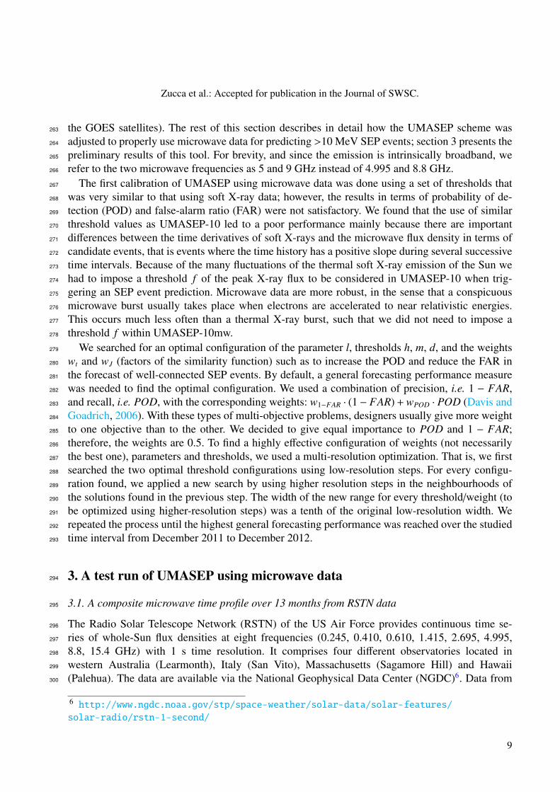
Fig. 7. UMASEP prediction web page for 2012 July 17: the upper and lower panel show the SEPprediction using soft X-rays and microwaves, respectively.
shown in the top panel of Figure 7. The microwave burst had a slowly evolving time profile, with440
a rise from start to peak over about 40 min, a flat high-frequency spectrum from 5 to 15 GHz, with441
a peak flux density around 40 sfu. This is typical of thermal bremsstrahlung. Because of the slow442
rise of the microwave time profile, only a rather weak correlation is found with the time derivative443
of the proton intensity profile. This correlation is below the similarity threshold smax, and no SEP444
forecast is issued by the UMASEP-10mw system, as shown in the lower panel of Figure 7.445
On 2012 Sep 28 an SEP event was preceded by a soft X-ray burst of class C3. This is below446
the UMASEP-10 threshold for event amplitudes (parameter f ), and no SEP event was predicted447
based on the soft X-rays (top panel of Figure 8). The microwave emission at 5 and 9 GHz was again448
thermal bremsstrahlung, with a rather low peak flux density (about 20 sfu at 9 GHz), but a faster449
rise from background to peak (within 20 min) than on 2012 Jul 17. The thermal bremsstrahlung450
17

Zucca et al.: Accepted for publication in the Journal of SWSC.
Fig. 8. UMASEP prediction web page for 2012 September 27: the upper and lower panel show theSEP prediction using soft X-rays and microwaves, respectively.
microwaves predicted the SEP event on Sep 28 (Fig. 8, bottom panel), unlike the thermal soft X-451
rays. This success is due to the faster rise of the microwave profile, which generated a correlation452
with the time derivative of the proton intensity above the similarity threshold smax, leading to a453
correct forecast of an SEP event.454
We finally discuss the large SEP event of 2012 May 17, which was successfully predicted by455
both UMASEP-10 and UMASEP-10mw, but with a very short warning time of only 5 min. It was456
missed by the original calibration of the UMASEP-10mw procedure: the microwave burst triggered457
a forecast, but this came after the SEP intensity exceeded the NOAA threshold (bottom panel of458
Figure 9). The short warning time is the result of a very fast arrival of the first SEPs, together with459
a steep rise of the time profile.460
18

Zucca et al.: Accepted for publication in the Journal of SWSC.
Fig. 9. UMASEP prediction web page for 2012 May 17: the upper and lower panel show the SEPprediction using soft X-rays and microwaves, respectively.
5. Summary and discussion461
An experimental run of the UMASEP prediction scheme of the occurrence of SEP events was462
presented, using microwave data as an identification of connection to a solar particle source. The463
key findings for a thirteen months period from December 2011 to December 2012 are the following:464
– The probability of detection is the same as in the traditional UMASEP scheme, where the deriva-465
tive of the soft X-ray time profile is correlated with the SEP intensity.466
– The false-alarm ratio is reduced to zero by the microwave data at both frequencies considered (5467
and 9 GHz).468
19

Zucca et al.: Accepted for publication in the Journal of SWSC.
– The warning time obtained with the microwave light curves is slightly improved with respect to469
soft X-rays (30.7 vs 26.4 min).470
The forecasting scheme using microwaves fails when the microwave emission is thermal and471
slowly rising (2012 June 17). Both soft X-ray based and microwave-based forecasts fail when the472
proton time profile rises slowly (2012 July 07). Both give only short warning times when the SEPs473
arrive very rapidly after the solar event (2012 May 17). Somewhat surprisingly, the forecasting474
seems to work on occasion even when the microwave emission is thermal bremsstrahlung, pro-475
vided its rise is not too slow (2012 September 27-28). This depends of course on the calibration476
of the internal parameters of the UMASEP scheme, which in turn depend on the fluctuations of477
the detected microwave signal. Microwave bursts, be they non-thermal gyrosynchrotron emission478
or thermal bremsstrahlung, are rarer than thermal soft X-ray bursts. If the latter are used in SEP479
forecasting, an empirical threshold must be imposed on the peak flux of the soft X-ray bursts to480
discard the ubiquitous small events. This turns out to not be necessary for microwave bursts.481
The comparatively rare occurrence of the microwave bursts probably explains the low false-alarm482
ratio. Spurious fluctuations of the microwave data then appear as the main problem of the method:483
baseline drifts due to erroneous antenna pointing or receiver instabilities, sudden jumps and slow484
fluctuations of the background with an amplitude well above the noise level led us to carefully485
calibrate the threshold associated with the minimum value of the background-subtracted microwave486
flux density to be considered. Part of these data problems could be corrected by a more careful487
cleaning. But a sophisticated and reliable data analysis is hardly possible in real time. Therefore a488
better controlled operation of the radio instruments appears mandatory if one wants to use them for489
an automated prediction scheme of SEP events in an operational service.490
Conclusions drawn here for the microwave emission probably pertain to hard X-rays, too. Hard491
X-ray time profiles are known to be similar to the time profiles of gyrosynchrotron microwaves.492
They do not show the thermal bremsstrahlung counterpart sometimes observed in the microwave493
time profiles. Since it is currently not possible to construct long uninterrupted time profiles of solar494
hard X-ray emission, we cannot test their predictive performance. A possible inconvenience is the495
sensitivity of the detectors to energetic particles, especially electrons, which contaminate observa-496
tions taken outside the Earth’s magnetosphere. This can be seen, for instance, in X-ray observations497
from the International Sun-Earth Explorer mission (ISEE-3) located at the L1 Lagrange point in498
Figure 1 of Kane et al. (1985). Figure 4 of Kuznetsov et al. (2011) illustrates a similar contamina-499
tion effect on a gamma-ray detector in polar orbit by solar and magnetospheric protons during the500
2003 Oct 28 event.501
The radio observations exploited in the present work are carried out with rather simple patrol502
instruments, which monitor the whole Sun flux density using parabolic antennas with a typical size503
of 1 metre. Such data are presently not provided in real time, but there is no technical obstacle to do504
so. If a reliable calibration and stable and reliable antenna operations can be achieved, microwave505
patrol observations will be a significant addition to our ability to predict the occurrence of SEP506
events. As attractive as microwave observations may be, they are limited to activity on the Earthward507
part of the solar disk or possibly just behind the western limb. The practical consequences of this508
limitation on the SEP impact are somewhat uncertain, because the intensity of SEPs at the Earth509
decreases significantly with increasing distance of the parent active region from W 100. In any510
case the limitation is shared with present soft X-ray observations, but can be overcome in principle511
20

Zucca et al.: Accepted for publication in the Journal of SWSC.
by placing a spacecraft in an adequate vantage point. While space-borne microwave observations512
are conceivable, the tool will then of course cease to be a cheap alternative to the X-rays.513
Acknowledgements. This research received funding from the European Union’s Horizon 2020 research and514
innovation programme under grant agreement No 637324 (HESPERIA project). It was also supported by515
the Agence Nationale pour la Recherche (ANR/ASTRID, DGA) project Outils radioastronomiques pour516
la meteorologie de l’espace (ORME, contract No. ANR-14-ASTR-0027) and by the French space agency517
CNES. The work is based on radio data from the RSTN network (provided through NGDC) and the Nobeyama518
Radio Polarimeters (NoRP). NoRP are operated by Nobeyama Radio Observatory, a branch of National519
Astronomical Observatory of Japan. Supporting information was provided by the Radio Monitoring web520
site maintained at Paris Observatory with support by CNES. The authors acknowledge detailed and helpful521
comments by the referees. PZ and KLK acknowledge helpful discussions with G. Trottet. The editor thanks522
Arik Posner and an anonymous referee for their assistance in evaluating this paper.523
References524
Aran, A., B. Sanahuja, and D. Lario. SOLPENCO: A solar particle engineering code. Adv. Space Res., 37,525
1240–1246, 2006. 10.1016/j.asr.2005.09.019.526
Aran, A., B. Sanahuja, and D. Lario. Comparing proton fluxes of central meridian SEP events with those527
predicted by SOLPENCO. Adv. Space Res., 42, 1492–1499, 2008. 10.1016/j.asr.2007.08.003.528
Balch, C. C. Updated verification of the Space Weather Prediction Center’s solar energetic particle prediction529
model. Space Weather, 6, S01,001, 2008. 10.1029/2007SW000337.530
Belov, A. Properties of solar X-ray flares and proton event forecasting. Adv. Space Res., 43(4), 467–473,531
2009. 0.1016/j.asr.2008.08.011.532
Davis, J., and M. Goadrich. The relationship between precision-recall and ROC curves. In W. Cohen533
and A. Moore, eds., Proceedings of the Twenty-Third International Conference on Machine Learning534
(ICML’06), vol. 148 of ACM Int. Conf. Proc. Ser., 233–240. Assoc. for Comput. Mach., 2006.535
10.1145/1143844.1143874.536
Dennis, B. R., and D. M. Zarro. The Neupert effect - What can it tell us about the impulsive and gradual537
phases of solar flares? Sol. Phys., 146, 177–190, 1993. 10.1007/BF00662178.538
Dierckxsens, M., K. Tziotziou, S. Dalla, I. Patsou, M. S. Marsh, N. B. Crosby, O. Malandraki, and539
G. Tsiropoula. Relationship between solar energetic particles and properties of flares and CMEs: sta-540
tistical analysis of solar cycle 23 events. Sol. Phys., 290, 841–874, 2015. 10.1007/s11207-014-0641-4,541
1410.6070.542
Dresing, N., R. Gomez-Herrero, B. Heber, A. Klassen, O. Malandraki, W. Droge, and Y. Kartavykh.543
Statistical survey of widely spread out solar electron events observed with STEREO and ACE with special544
attention to anisotropies. Astron. Astrophys., 567, A27, 2014. 10.1051/0004-6361/201423789.545
Garcia, H. A. Forecasting methods for occurrence and magnitude of proton storms with solar soft X-rays.546
Space Weather, 2, S02,002, 2004. 10.1029/2003SW000001.547
21

Zucca et al.: Accepted for publication in the Journal of SWSC.
Garcıa-Rigo, A., M. Nunez, R. Qahwaji, O. Ashamari, P. Jiggens, G. Perez, M. Hernandez-Pajares, and548
A. Hilgers. Prediction and warning system of SEP events and solar flares for risk estimation in space launch549
operations. Journal of Space Weather and Space Climate, 6(27), A28, 2016. 10.1051/swsc/2016021.550
Holman, G. D., M. J. Aschwanden, H. Aurass, M. Battaglia, P. C. Grigis, E. P. Kontar, W. Liu, P. Saint-551
Hilaire, and V. V. Zharkova. Implications of X-ray observations for electron acceleration and propagation552
in solar flares. Space Sci. Rev., 159, 107–166, 2011. 10.1007/s11214-010-9680-9, 1109.6496.553
Kahler, S. W., E. W. Cliver, and A. G. Ling. Validating the proton prediction system (PPS). J. Atmos.554
Solar-Terr. Phys., 69, 43–49, 2007. 10.1016/j.jastp.2006.06.009.555
Kane, S. R., P. Evenson, and P. Meyer. Acceleration of interplanetary solar electrons in the 1982 August 14556
flare. Astrophys. J., 299, L107–L110, 1985. 10.1086/184590.557
Klein, K.-L., S. Krucker, G. Lointier, and A. Kerdraon. Open magnetic flux tubes in the corona and the trans-558
port of solar energetic particles. Astron. Astrophys., 486, 589–596, 2008. 10.1051/0004-6361:20079228.559
Kuznetsov, S. N., V. G. Kurt, B. Y. Yushkov, K. Kudela, and V. I. Galkin. Gamma-ray and high-energy-560
neutron measurements on CORONAS-F during the solar flare of 28 October 2003. Sol. Phys., 268, 175–561
193, 2011. 10.1007/s11207-010-9669-2.562
Laitinen, T., and S. Dalla. Energetic Particle Transport across the Mean Magnetic Field: Before Diffusion.563
Astrophys. J., 834, 127, 2017. 10.3847/1538-4357/834/2/127, 1611.05347.564
Laurenza, M., E. W. Cliver, J. Hewitt, M. Storini, A. G. Ling, C. C. Balch, and M. L. Kaiser. A technique565
for short-term warning of solar energetic particle events based on flare location, flare size, and evidence of566
particle escape. Space Weather, 7, S04,008, 2009. 10.1029/2007SW000379.567
Lee, M. A., R. A. Mewaldt, and J. Giacalone. Shock acceleration of ions in the Heliosphere. Space Sci. Rev.,568
173, 247–281, 2012. 10.1007/s11214-012-9932-y.569
Mann, G., F. Jansen, R. J. MacDowall, M. L. Kaiser, and R. G. Stone. A heliospheric density model and type570
III radio bursts. Astron. Astrophys., 348, 614–620, 1999.571
Marsh, M. S., S. Dalla, M. Dierckxsens, T. Laitinen, and N. B. Crosby. SPARX: A modeling system572
for Solar Energetic Particle Radiation Space Weather forecasting. Space Weather, 13, 386–394, 2015.573
10.1002/2014SW001120, 1409.6368.574
Masson, S., P. Demoulin, S. Dasso, and K.-L. Klein. The interplanetary magnetic structure that guides solar575
relativistic particles. Astron. Astrophys., 538, A32, 2012. 10.1051/0004-6361/201118145, 1110.6811.576
Nakajima, H., H. Sekiguchi, M. Sawa, K. Kai, and S. Kawashima. The radiometer and polarimeters at 80,577
35, and 17 GHz for solar observations at Nobeyama. Publ. Astron. Soc. Jpn., 37, 163–170, 1985.578
Neupert, W. M. Comparison of solar X-ray line emission with microwave emission during flares. Astrophys.579
J., 153, L59–L64, 1968. 10.1086/180220.580
Nunez, M. Predicting solar energetic proton events (E > 10 MeV). Space Weather, 9, 07003, 2011.581
10.1029/2010SW000640.582
Nunez, M. Real-time prediction of the occurrence and intensity of the first hours of >100 MeV solar energetic583
proton events. Space Weather, 13, 807–819, 2015. 10.1002/2015SW001256.584
22

Zucca et al.: Accepted for publication in the Journal of SWSC.
Posner, A. Up to 1-hour forecasting of radiation hazards from solar energetic ion events with relativistic585
electrons. Space Weather, 5, S05001, 2007. 10.1029/2006SW000268.586
Richardson, I. G., and H. V. Cane. Particle flows observed in ejecta during solar event onsets and their impli-587
cation for the magnetic field topology. J. Geophys. Res., 101, 27,521–27,532, 1996. 10.1029/96JA02643.588
Richardson, I. G., T. T. von Rosenvinge, H. V. Cane, E. R. Christian, C. M. S. Cohen, A. W. Labrador, R. A.589
Leske, R. A. Mewaldt, M. E. Wiedenbeck, and E. C. Stone. > 25 MeV proton events observed by the High590
Energy Telescopes on the STEREO A and B spacecraft and/or at Earth during the first seven years of the591
STEREO mission. Sol. Phys., 289, 3059–3107, 2014. 10.1007/s11207-014-0524-8.592
Smart, D. F., and M. A. Shea. Modeling the time-intensity profile of solar flare generated particle fluxes in593
the inner heliosphere. Adv. Space Res., 12, 303–312, 1992. 10.1016/0273-1177(92)90120-M.594
Souvatzoglou, G., A. Papaioannou, H. Mavromichalaki, J. Dimitroulakos, and C. Sarlanis. Optimizing the595
real-time ground level enhancement alert system based on neutron monitor measurements: Introducing596
GLE Alert Plus. Space Weather, 12, 633–649, 2014. 10.1002/2014SW001102.597
Torii, C., Y. Tsukiji, S. Kobayashi, N. Yoshimi, H. Tanaka, and S. Enome. Full-automatic radiopolarimeters598
for solar patrol at microwave frequencies. Proceedings of the Research Institute of Atmospherics, Nagoya599
University, 26, 129–132, 1979.600
23