1

EXISTENCE OF MEIR-KEELER FIXED POINT

RESULTS IN VARIOUS SPACES

MTH645: DISSERTATION-II

SUBMITTED BY SUPERVISED BY

Sandeep Kaur(11501294) Dr. Manoj Kumar

SCHOOL OF CHEMICAL ENGINEERING AND PHYSICAL

SCIENCES DEPARTMENT OF MATHEMATICS

LOVELY PROFESSIONAL UNIVERSITY JALANDHAR,

PUNJAB

2

Declaration of Authorship

I, Sandeep Kaur, declare that this thesis titled, “Existence of Meir-Keeler fixed point results in

various spaces” and the work presented in it are my own. I confirm that:

This work was done wholly or mainly while in candidature for a research degree at this

University.

Where any part of this project has previously been submitted for a degree or any other

qualification at this University or any other institution, this has been clearly stated.

Where I have consulted the published work of others, this is always clearly attributed.

Where I have quoted from the work of others, the source is always given. With the

exception of such quotations, this project is entirely my own work.

I have acknowledged all main sources of help.

Where the project is based on work done by myself jointly with others, I have made clear

exactly what was done by others and what I have contributed myself.

Signed:

Author: SANDEEP KAUR

Registration No.: 11501294

Date: April 2017

3

Certificate

This is to certify that SANDEEP KAUR has completed Project titled “Existence of Meir-Keeler

fixed Point results in various Spaces” under my guidance and supervision. To the best of my

knowledge, the present work is the result of her original investigation and study. No part of the

project has ever been submitted for any other degree at any University.

The project is fit for the submission and the partial fulfillment of the conditions for the award of

Master of Science in Mathematics.

Signed:

Supervisor: Dr. MANOJ KUMAR

Associate Professor

Date: April 2017

4

“Thanks to my solid academic training, today I can write hundreds of words on virtually any

topic without possessing a shred of information, which is how I got a good job in journalism.”

Dave Barry

5

Abstracts

In this paper, first of all we introduce the new notion of generalized 𝛽 − 𝜓 −asymmetric Meir-

Keeler contractive mapping in G-metric spaces and prove certain fixed point theorems in the

setting of these spaces. Further, we introduce a new notion of generalized Meir-Keeler 𝜓 − 𝛼-

contraction in partial metric spaces and then we prove some fixed point theorems in these spaces

through rational expressions. Some results in the literature are also generalized from our results.

6

Acknowledgement

It is great pleasure for me to present the project report on “Existence of Meir-Keeler fixed

Point results in various Spaces”. Every work accomplished is a pleasure, a sense of fulfillment.

However many people always motivate, criticize and appreciate a work with their objective ideas

and opinions. I would like to use this opportunity to thank all, who have directly or indirectly

helped us to complete the capstone-1.

Firstly, I would like to thank Dr. Manoj Kumar. I never would’ve completed my capstone-1

without the help of Dr. Manoj Kumar. It is my pride and privilege to express my sincere thanks

and deep sense of gratitude for his valuable advice, splendid supervision and constant patience

through which this work was able to take the shape in which it has been presented.

Next, I would like to thank all people who gave their valuable time and feedback to this project. I

would also like to thank my collage for supporting us with resources which beyond any doubt

have helped me.

At last I would prefer to specify my deep feeling to our head of department Mr. Kulwinder Singh

and head of school Dr. Ramesh Thakur for providing all necessary facilities and inspiring.

Sandeep Kaur

Lovely Professional University, Punjab

7

CONTENTS

Declaration of Authorship 2

Certificate 3

Abstract 5

Acknowledgement 6

Chapter 1 Introduction

1.1 Background of fixed point theory 8

1.2 Definitions 8

1.3 Examples 8

1.4 Significance of fixed point theory 9

Chapter 2 Review of Literature

2.1 literature review 11

2.2 Applications of fixed point theory 13

2.2.1 In Analysis 13

2.2.2 Image Compression 13

2.2.3 Page Rank Algorithm 14

2.2.4 Game Theory 15

2.2.5 To solve differential and integral equations 15

Chapter 3 Main Results

3.1 Objective of the study 17

3.2 G-metric Space 17

3.3 Partial Metric Space 21

Bibliography 27

8

CHAPTER-1

INTRODUCTION

In the study of mathematics, fixed points are an important part of nonlinear functional analysis.

The study of fixed points has been at the center of energetic research activity in the last decades

where the mappings satisfying certain contractive conditions in different abstract spaces. The

Banach contraction mapping principle is one of the incipient and basic results in this direction. In

a complete metric space each contraction has a unique fixed point. In many mathematical

problems the existence of solution and existence of fixed point are equal. Therefore the existence

of fixed point is foremost significant in different fields of mathematics and other sciences. Fixed

point results gives situations under which the maps have solutions. The theory of fixed points

thus a great and delighted combination of analysis (pure and applied). It has been developed

through various spaces such as metric space, topological space, fuzzy metric space etc.

1.1 Background of fixed point theory

Fixed point theory itself is a beautiful mixture of analysis, topology and geometry. Over past 60

years, fixed point theory has been established itself as a very most powerful and considerable

tool in the study of nonlinear phenomena. In general, fixed point techniques have been applied in

diverse fields such as in biology, chemistry, economics, engineering, game theory and physics.

The point at which the y = f(x) and the line y = x intersects gives the solution of the curve, and

the point of intersection is the fixed point of the curve. The usefulness of the concrete

applications has increased enormously due to the development of accurate techniques for

computing fixed points.

Fixed point theory is rapidly moving into the mainstream of mathematics mainly because of its

applications in diverse fields which include numerical methods like Newton-Raphson method,

establishing Picard’s Existence theorem, existence of solution of integral equations and a system

of linear equations.

Definition 1.2 Let X be a non-empty set and F: X → X be a mapping. A solution of the equation F(x) =

x is called a fixed point of F.

In other words, a fixed point is a point which does not change under a certain map.

Example 1.3 Examples of fixed point are as follows:

(a) A translation mapping has no fixes point, that is,

9

G(x) = x + 1 for all x ∈ R.

(b) A mapping T: R ⟶ R defined by Tx = 𝑥

𝑘 − (k −1), where k is a positive integer,

Then x = −k is the unique fixed point.

(c) A mapping T: R → R defined by T(x) = x, has infinitely many fixed points, i.e., every

point of domain is a fixed point of T.

Therefore, from the above examples one can conclude that a mapping may have a unique fixed

point, it may have more than one or even infinitely many fixed point. Theorems dealing with the

existence and construction of a solution to an operator equation T(x) = x form the part of fixed

point theory. In functional analysis fixed point theory is divided mainly into four branches:

Set theoretic fixed point theory

Metric fixed point theory

Topological fixed point theory

Fuzzy topological fixed point theory

1.4 Significance of Fixed Points

Fixed points are the points which remain invariant under a map/transformation. Fixed points tell

us which parts of the space are pinned in plane, not moved, by the transformation. The fixed

points of a transformation restrict the motion of the space under some restrictions. We note that

fixed point problems and root finding problems f(x) = 0 are equivalent.

Now, we state a result which gives us the guarantee of existence of fixed points.

Suppose g is continuous self map on [a, b]. Then, we have the following conclusions:

(1) If the range of the mapping y = g(x) satisfies y ∈ [a, b] for all x ∈ [a, b], then g has

a fixed point in [a, b].

(2) Suppose that gˊ(x) is defined over (a, b) and that a positive constant k < 1 exists with

| gˊ(x)|≤ 𝑘 for all x ∈ (a, b), then g has a unique fixed point p in [a, b].

Now, suppose that (X, d) be a complete metric space and T: X → X be a map. The mapping T

satisfies a Lipschitzs condition with constant 𝛼 ≥ 0 such that d(Tx, Ty) ≤ 𝛼 d(x, y), for all x, y

in X. For different values of 𝛼, we have the following cases:

(a) T is called a contraction mapping if 𝛼 < 1;

(b) T is called non-expansive if 𝛼 ≤ 1;

(c) T is called contractive if 𝛼 = 1.

10

It is clear that contraction ⟹ 𝑐𝑜𝑛𝑡𝑟𝑎𝑐𝑡𝑖𝑣𝑒 ⟹ 𝑛𝑜𝑛 − 𝑒𝑥𝑝𝑎𝑛𝑠𝑖𝑣𝑒 ⟹ 𝐿𝑖𝑝𝑠𝑐𝑕𝑖𝑡𝑧.

However, converse is not true in either case as:

(1) The identity map I: X ⟶ X, where X is a metric space, is non-expansive but not

contractive.

(2) Let X = [0,∞) be a complete metric space equipped with the metric of absolute value.

Define, f: X → X given by f(x) = x +1 𝑥 . Then f is contractive map, while f is not

contraction.

Thus, fixed points give a way to establish the existence of a solution to a set of equations.

If the system of equation for which a solution is solved is in the form of p(x) = 0.

Then, the function p will defined as

p(x) =q(x) –x

A fixed point of q is a solution to p(x) = 0.

11

CHAPTER-2

Review of Literature

2.1 Literature Review

The origin of fixed point theory was basically for the successive approximation to establish the

existence and uniqueness of solutions, for the differential and integral equations.

There are mainly two types of fixed point theorems: constructive fixed point theorems and non-

constructive fixed point theorems. Constructive fixed point theorems are those theorems that

provide the existence of solution as well as yield an algorithm such as Banach fixed point

theorem. On the other hand non-constructive theorems define estimate of the number of fixed

points such as Brouwer’s fixed point theorem. Poincare was the first to work in this field of fixed

points, in 1886. Then in 1912, Brouwer gave the fixed point theorem for the solution of the

equation g(x) = x. He also proved fixed point theorem for a square, a sphere and their n-

dimensional counter parts that was further extended by Kakutani. Several proofs of Brouwer’s

theorem are given by others. This theorem just gave information about the solution that exists but

no more information about the uniqueness and how to determine the solution. It gives no

information about the place of fixed point where it is located. Throughout this, Banach gave his

principle which was judged as one of the primary principle in the field of functional analysis.

Banach’s contraction principle plays vital role in the existence and uniqueness theorems in

different branches of sciences. The most useful feature of this principle is that it gives the

existence, uniqueness and the convergence of the sequence of successive approximation to a

solution of the problem. In 1992, Banach beared out that a contraction mapping in the field of

complete metric space have a unique fixed point. After that it was studied and extended by

Kannan. Fixed point theory is integrative topic that is useful in various directions of mathematics

and mathematical sciences. Mainly, there are two important fixed point theorems: one is Brouwer’s

(1912), and the other Banach’s (1922) fixed point theorem. Brouwer’s fixed point theorem is existential

by its nature.

The elegant Banach’s fixed point theorem solves:

a) The problem on the existence of a unique solution to an equation,

b) Gives a practical method to obtain approximate solution and

12

c) Gives an estimate of such solutions.

The applications of the Banach’s fixed theorem and its generalization are very important in

diverse disciplines of mathematics, statistics, engineering and economics.

In 1922, Banach [2] proved a fixed-point theorem and called it Banach Fixed Point Theorem or

Banach Contraction Principle which is considered as the mile stone in fixed point theory. This

theorem provides a technique for solving a variety of applied problems in mathematical sciences

and engineering. This theorem was generalized and improved in different ways by various

authors. Many important proofs in nonlinear analysis and optimization involve applications of

various fixed point theorems. In 1909, Luitzen Brouwer has proved the first fixed point theorem

called Brouwer’s theorem. The notion of partial metric space was introduced by Matthews in

1992. In fact, a partial metric space is a generalization of usual metric spaces in which d(x, x) are

no longer necessarily zero. Thus, a partial metric space can be defined to be a partial metric

space in which each self-distance is zero. This principle has had many applications but it suffers

from one drawback – the definition requires that T be continuous throughout X. Therefore, from

the above examples one can conclude that a mapping may have a unique fixed point, it may have

more than one or even infinitely many fixed points and it may not have any fixed point.

With the discovery of computer and development of new software’s for speedy and fast

computing, a new dimension has been given to fixed point theory. New field of study generated

like applied mathematics, numerical analysis and algorithms. Fixed point theory has become the

subject of scientific research. As the introduction of Jungck’s fixed point theorem on

commutative mappings and then relaxing the condition of commutatively by weak

commutatively by the results of Sessric followed by the work a and similar concepts new turn

takes place in the development of fixed point theory. Drastic chances took place with the work of

Ciric followed by the work of Rhoades, Krik on non-expansive mappings and the work of Park

and Sadovski B. have made valuable contribution by considering new types of mapping

conditions.

After the work of Mann and Ishikawa in the field of fixed point theory took a new direction for

approximating fixed point and convergence of iterative of sequences. Many other gave many

results in this field. The reason behind this kind of work is that a few types of approximate

numerical solution is required when the equation may not be able to give exact solution. It is

seen from the above history and theory of fixed points that the fixed points can be managed

13

either by modifying the nature of mappings or by emphasizing upon the studies on the structure

of the space and its topological characteristic. Fixed point theory is a major research area of new

researches and advancements. New results and researches are given by various authors day by

day and thus it becomes a important topic of study.

2.2 APPLICATIONS OF FIXED POINT THEORY

Fixed point techniques have been put in disparate fields like in biology, chemistry, economics,

engineering, medical sciences, classical analysis, functional analysis, integral equations,

differential equations, partial differential equation, general and applied technology, game theory

and physics. In many fields, equilibrium and stability are the key concepts that can be

represented in the way of fixed points. For example, economics, game theory. Also, many

compilers that convert normal language to programming language use fixed point computations

for program analysis. For example, data flow analysis. Some of the examples of fixed point

theory are as follows:

2.2.1 In Analysis

The most important example of Banach fixed point theorem is the proof of:

1. The existence of solution of differential equations.

2. The uniqueness of solutions of differential equation.

2.2.2 Application to image compression

The right way to save an image in memory is to store the color of each pixel. There are two

problems with this method:

a) It demands a huge quantity of memory.

b) If we try to expand the image, for instance for using it in a large poster, then the pixels

will become larger squares and we will be missing information on how to fill the details

in these squares

It is to encode less information than the original image so that the eye cannot see that image

observed is determined. Internet has increased the need for good image compression. Indeed,

images slow down navigation on the web quite significantly. So for internet navigation, it is

good to have images encoded in files as small as possible.

14

There are several different ways in which image files can be compressed. For Internet use,

generally the two more special quality compressed graphic image formats are the JPEG

format and the GIF format. The JPEG method is more often used for photographs, while the

GIF format is usually used for line art and other images in which geometric shapes are

comparatively not complicated. More techniques for image compression include the use of

fractals and wavelets. These methods have not given much acceptance for use on the internet

as of this writing.

There is another method, which has remained more experimental. This method was given by

Barnsley, and it is called iterated function systems. The main motive behind this method is to

approximate an image by geometric objects. The geometric objects are not limited to lines

and smooth curves, but also the fractal objects like the fern, the Sierpinski Carpet, the

Menger Sponge , and many more.

.

2.2.3 The Page Rank algorithm

The PageRank algorithm is an amazing application of Banach fixed point theorem. PageRank is

an algorithm that is used by Google search to rank websites in their search engine results.

Larry Page is an inventor of PageRank. He is also the founder of Google. He invented it in 1998.

The idea of PageRank was that, the significance of a web page can be decided by looking at the

pages that link to it. It is a way of calculating the importance of website pages. In PageRank

algorithm, a fixed point of a linear operator ℝ𝑛 is computed which is contraction, and this fixed

point yields the ordering of pages.

Google is successful due to because a search engine arrives from its algorithm: the page rank

algorithm. In this algorithm, one can computes a fixed point of linear operator on eculiden space

which is a contraction, and this fixed point yields the arranging of the pages.

15

2.2.4 GAME THEORY:

Consider a game with n≥2 players, and the assumption that the players do not cooperate among

themselves. Each player follows a strategy, in dependence of the strategies of the other players.

Denote the set of all possible strategies of the 𝑞𝑡𝑕 player by𝑄𝑞 , and set 𝑄 = 𝑄1 × …× 𝑄𝑛 . An

element 𝑎 ∈ 𝑄 is called a strategy profile. For each q, let 𝑔𝑞 :𝑄 → ℝ be the loss function of the

𝑞𝑡𝑕 player. If

𝒈𝒒(𝒂)𝒏𝒒=𝟏 = 0, 𝑓𝑜𝑟 𝑎𝑙𝑙 𝑎𝜖 𝑄

the game is said to be of zero-sum. The aim of each player is to minimize his loss,

Or, equivalently, to maximize his gain

2.2.5 TO SOLVE DIFFERENTIAL EQUATIONS AND INTEGRAL

EQUATIONS:

Let g(x, y) be a continuous real-valued function on closed interval [a, b]×[c ,d]. The Cauchy

Initial value problem is to find a continuous differential function y on [a, b] satisfying the

differential equation

𝑑𝑦

𝑑𝑥= 𝑝 𝑥, 𝑦 ,𝑦 𝑥0 = 𝑦0 (1)

Consider the Banach space C[a ,b] of continuous real-valued functions with supremum norm

defined by ∥ 𝑦 ∥ = sup 𝑦 𝑥 𝑥𝜖 𝑎,𝑏 .

On integrating, we obtain an integral equation

𝑦 𝑥 = 𝑦0 + ∫ 𝑝(𝑡,𝑦(𝑡))𝑑𝑡𝑥

𝑥0 (2)

The problem (1) is equivalent the problem solving the integral equation (2).

We define an integral operator T: C[a, b]→C[a ,b] by

𝑇𝑦 𝑥 = 𝑦0 + 𝑝(𝑡, 𝑦(𝑡))𝑑𝑡𝑥

𝑥0

Thus, a solution of Cauchy initial value problem (1) corresponds with a fixed point of T. One

may easily check that if T is contraction, then the problem (1) has a unique solution.

The integral equations occur in applied mathematics, engineering and mathematical physics.

They also arise as representation formulas in the solution of differential equations. The equations

16

𝑞 𝑥 = 𝑠 𝑥,𝑦 𝑞 𝑦 𝑑𝑦,𝑏

𝑎

𝑞 𝑥 = 𝑝 𝑥 + 𝑠 𝑥,𝑦 𝑞 𝑦 𝑑𝑦,𝑏

𝑎

𝑞 𝑥 = 𝑠 𝑥,𝑦 𝑞(𝑦)2𝑑𝑦,𝑏

𝑎

Here q is an unknown function and all other functions are known are called integral equations.

The most general linear integral equation in y(x) can be written as

𝑕 𝑥 𝑦 𝑥 = 𝑔 𝑥 + 𝑘 𝑥, 𝑡 𝑦(𝑡)𝑑𝑡𝑏(𝑥)

𝑎

When b(x) = x, this equation is called Volterra integral equation.

𝑕 𝑥 𝑠𝑦 𝑥 = 𝑔 𝑥 + 𝑘 𝑥, 𝑡 𝑦(𝑡)𝑑𝑡𝑥

𝑎

.

17

CHAPTER-3

Fixed Point Theorems for Meir- Keeler-type mappings in G-metric spaces and

Partial metric spaces

3.1Objectives of the study

Our objective was to meet the following objectives:

To design a framework to survey the study of fixed point in partial metric spaces as studied by

other researchers using

(1) Triangular-𝛼 -admissible mapping

(2) Generalized 𝛽 -asymmetric Meir-Keeler contractive conditions.

(3) Meir-Keeler-type 𝜙 − 𝛼 − contractions on partial metric spaces.

(4) Partial Metric Spaces involving Rational Expressions.

Metric Space: let X be a non-empty set. Let d: X × X → ℝ be a map. Then (X, d) is said to be

metric space if the following conditions holds:

(i) d(x, y) ≥ 0 and d(x,y) = 0 ⇔ x=y

(ii) d(x, y) = d(y, x)

(iii) d(x, y) ≤ d(x, z) + d(z, y) for all x, y, z ∈ X.

G-metric space: let X be a non-empty set. Let a function G: X × X × X → ℝ+. Then a pair

(X, G) is called a G-metric space if the following conditions are satisfied:

(i) G(x, y, z) = 0 if x = y = z;

(ii) G(x, y, y) > 0 for any x, y ∈ X with x ≠ y;

(iii) G(x, x, y) ≤ G(x, y, z) for any x, y, z ∈ X with y ≠ z;

(iv) G(x, y, z) = G(x, y, z) = G(x, y, z) =…, symmetry in all three variables;

(v) G(x, y, z) ≤ G(x, a, a) + G(a, y, z) for any x, y, z, a∈ X

Meir-Keeler contractive mapping:

The Banach contraction mapping principle is one of the pivotal results of analysis. It is widely

considered as the source of metric fixed point theory. Generalization of this principle has been a

heavily investigated branch of research. In particular, one of the remarkable notions in fixed

point theory is Meir-Keeler contraction mapping which is as follows:

18

Let (X, d) be a complete metric space and T: 𝑋 → 𝑋. Assume that, for every 휀 > 0, there exists

𝛿( 휀) > 0 such that

x, y ∈ X; 휀 ≤ d( x, y) < 휀 + 𝛿 ⇒ d( Tx, Ty) < 휀.

Then T has a unique fixed point x* ∈ 𝑋 and 𝑇𝑛𝑥 → 𝑥 ∗ 𝑎𝑠 𝑛 → ∞ for every x ∈ X, where 𝑇𝑛

denotes the nth order iterate of T.

Modified 𝜶 −𝝍 Asymmetric Meir-Keeler contractive Mappings: Let (X, d) be a metric

space and let 𝜓 be a non-decreasing, sub-additive altering distance function. Suppose that

f: X → X is a triangular 𝛼-admissible mapping satisfying the following condition:

For each 휀 > 0 there exists 𝛿 > 0 such that

휀 ≤ 𝜓(d(x, y)) < 휀 + 𝛿 implies 𝜓(d(fx, fy)) < 휀

For all x, y ∈ X with 𝛼(x, y) ≥ 1. Then f is called a modified 𝛼 − 𝜓 − Meir-Keeler contractive

mapping.

Theorem3.2 Let (X, G) be a G-complete G-metric space andΦ ∈ 𝜓. Suppose that T: X → 𝑋 is a

triangular 𝛼 −admissible and modified 𝛼 − Φ −asymmetric Meir-keeler contractive mapping.

Assume that there exists 𝑥0 ∈ 𝑋 such that 𝛼 𝑥0, 𝑇𝑥0 ≥ 1 and T is continuous, then T has a

fixed point.

𝑮𝒎 –Meir-Keeler -Contractive mappings: Let (X, G) be a G-metric space. Suppose that

f: X → X is a self-mapping satisfying the following condition:

for each 휀 > 0, there exists 𝛿 > 0 such that for all m ∈ ℕ, we have

ℰ ≤ 𝐺( x, 𝑓(𝑚 )𝑥,𝑦) < 휀 + 𝛿 implies G(fx, 𝑓(𝑚+1)𝑥, 𝑓𝑦) < 휀.

Then f is called a 𝐺𝑚 -Meir-Keeler contractive mapping.

Definition3.2 Let (Y, G) be a G-metric space and 𝜓 ∈ Ψ . Suppose that f is a self map satisfying

the following conditions:

For each 𝜖 > 0 there exists 𝛿 > 0 such that for all x, y ∈ Y and for all q ∈ ℕ, we have

휀 ≤ 𝜓(G(x,𝑓𝑞𝑥, 𝑦)) <휀 + 𝛿 implies 𝜓(G(fx,𝑓(𝑞+1)𝑥, 𝑓𝑦)) < 휀 for all x,y ∈ Y with 𝛽(𝑥, 𝑦) ≥ 1.

Then f is called generalized 𝛽 − 𝜓 − 𝑎𝑠𝑦𝑚𝑚𝑒𝑡𝑟𝑖𝑐 Meir Keeler contractive mapping.

Remark3.2.2 If f : Y→ Y is a 𝐺𝑚 Meir Keeler contractive mapping on a G metric space Y, then

𝜓 𝐺(𝑓𝑥, 𝑓 𝑞+1 𝑥,𝑓𝑦) < 𝜓(𝐺(𝑥, 𝑓𝑞𝑥,𝑦)) holds for all x,y ∈ 𝑋 and for all q∈ ℕ with

𝛽(𝑥, 𝑦) ≥ 1 when 𝜓(𝐺(𝑥, 𝑓𝑞𝑥, 𝑦)) > 0.

On the other hand if 𝜓 𝐺 𝑥,𝑓𝑞𝑥, 𝑦 = 0 then x = 𝑓𝑞𝑥 = 𝑦 and so

19

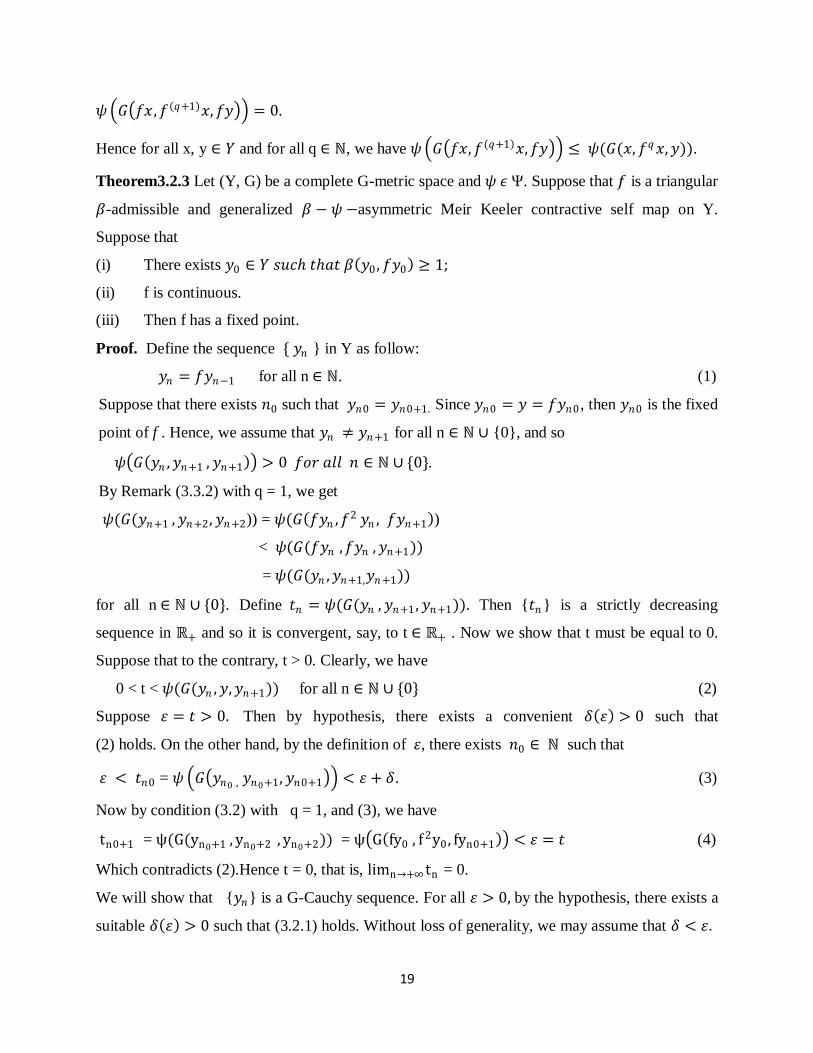
𝜓 𝐺 𝑓𝑥 ,𝑓 𝑞+1 𝑥,𝑓𝑦 = 0.

Hence for all x, y ∈ 𝑌 and for all q ∈ ℕ, we have 𝜓 𝐺 𝑓𝑥,𝑓 𝑞+1 𝑥,𝑓𝑦 ≤ 𝜓(𝐺(𝑥, 𝑓𝑞𝑥,𝑦)).

Theorem3.2.3 Let (Y, G) be a complete G-metric space and 𝜓 𝜖 Ψ. Suppose that 𝑓 is a triangular

𝛽-admissible and generalized 𝛽 − 𝜓 −asymmetric Meir Keeler contractive self map on Y.

Suppose that

(i) There exists 𝑦0 ∈ 𝑌 𝑠𝑢𝑐𝑕 𝑡𝑕𝑎𝑡 𝛽 𝑦0 , 𝑓𝑦0 ≥ 1;

(ii) f is continuous.

(iii) Then f has a fixed point.

Proof. Define the sequence { 𝑦𝑛 } in Y as follow:

𝑦𝑛 = 𝑓𝑦𝑛−1 for all n ∈ ℕ. (1)

Suppose that there exists 𝑛0 such that 𝑦𝑛0 = 𝑦𝑛0+1. Since 𝑦𝑛0 = 𝑦 = 𝑓𝑦𝑛0, then 𝑦𝑛0 is the fixed

point of f . Hence, we assume that 𝑦𝑛 ≠ 𝑦𝑛+1 for all n ∈ ℕ ∪ {0}, and so

𝜓 𝐺 𝑦𝑛 ,𝑦𝑛+1 , 𝑦𝑛+1 > 0 𝑓𝑜𝑟 𝑎𝑙𝑙 𝑛 ∈ ℕ ∪ {0}.

By Remark (3.3.2) with q = 1, we get

𝜓(𝐺(𝑦𝑛+1 , 𝑦𝑛+2, 𝑦𝑛+2)) = 𝜓(𝐺 𝑓𝑦𝑛 ,𝑓2 𝑦𝑛 , 𝑓𝑦𝑛+1 )

< 𝜓(𝐺(𝑓𝑦𝑛 ,𝑓𝑦𝑛 ,𝑦𝑛+1))

= 𝜓(𝐺(𝑦𝑛 ,𝑦𝑛+1,𝑦𝑛+1))

for all n ∈ ℕ ∪ {0}. Define 𝑡𝑛 = 𝜓(𝐺(𝑦𝑛 , 𝑦𝑛+1 , 𝑦𝑛+1)). Then {𝑡𝑛} is a strictly decreasing

sequence in ℝ+ and so it is convergent, say, to t ∈ ℝ+ . Now we show that t must be equal to 0.

Suppose that to the contrary, t > 0. Clearly, we have

0 < t < 𝜓(𝐺(𝑦𝑛 ,𝑦,𝑦𝑛+1)) for all n ∈ ℕ ∪ {0} (2)

Suppose 휀 = 𝑡 > 0. Then by hypothesis, there exists a convenient 𝛿 휀 > 0 such that

(2) holds. On the other hand, by the definition of 휀, there exists 𝑛0 ∈ ℕ such that

휀 < 𝑡𝑛0 = 𝜓 𝐺 𝑦𝑛0 , 𝑦𝑛0+1, 𝑦𝑛0+1 < 휀 + 𝛿. (3)

Now by condition (3.2) with q = 1, and (3), we have

tn0+1 = ψ(G(yn0+1 , yn0+2 , yn0+2)) = ψ G fy0 , f 2y0 , fyn0+1 < 휀 = 𝑡 (4)

Which contradicts (2).Hence t = 0, that is, limn→+∞ tn = 0.

We will show that {𝑦𝑛} is a G-Cauchy sequence. For all 휀 > 0, by the hypothesis, there exists a

suitable 𝛿 휀 > 0 such that (3.2.1) holds. Without loss of generality, we may assume that 𝛿 < 휀.

20

Since t = 0, there exist 𝑁 > ℕ such that

𝑡𝑛−1 = 𝜓 𝐺 𝑦𝑛−1, 𝑦𝑛 , 𝑦𝑛 < 𝛿 𝑓𝑜𝑟 𝑎𝑙𝑙 𝑛 ≥ 𝑁. (5)

We asserts that for any fixed k ≥ 𝑁, the condition

𝜓 𝐺 𝑦𝑘 , 𝑦𝑘+𝑝 , 𝑦𝑘+𝑝 ≤ 휀 𝑓𝑜𝑟 𝑎𝑙𝑙 𝑝 ∈ ℕ (6)

To prove it, we use the method of induction. By Remark (3.2.2) and (5), assertion (5) is satisfied

for p = 1. Suppose that (5) is satisfied for p = 1, 2,…, q for some q ∈ ℕ.

Now, for p = q+1, using (4), we obtain

𝜓 𝐺 𝑦𝑘−1 ,𝑓 𝑞+1 𝑦𝑘−1, 𝑦𝑘+𝑞 = 𝜓(𝐺(𝑦𝑘−1, 𝑦𝑘+𝑞 ,𝑦𝑘+𝑞))

≤ 𝜓(𝐺 𝑦𝑘−1, 𝑦𝑘 ,𝑦𝑘 + 𝐺(𝑦𝑘 , 𝑦𝑘+𝑞 ,𝑦𝑘+𝑞))

≤ 𝜓 𝐺 𝑦𝑘−1 , 𝑦𝑘 ,𝑦𝑘 + 𝜓(𝐺(𝑦𝑘 , 𝑦𝑘+𝑞 ,𝑦𝑘+𝑞))

< 휀 + 𝛿. (7)

𝜓(G(𝑦𝑘−1 ,𝑦𝑘+𝑞 , 𝑦𝑘+𝑞 )) ≥ 휀, 𝑡𝑕𝑒𝑛 by(3.2), we get

𝜓 𝐺 𝑦𝑘 , 𝑦𝑘+𝑞+1, 𝑦𝑘+𝑞+1 = 𝜓(𝐺(𝑓𝑦𝑘−1 ,𝑓 𝑞+2 𝑦𝑘−1 , 𝑓𝑦𝑘+𝑞)) < 휀

And hence (6) is satisfied.

If 𝜓 𝐺 𝑦𝑘−1, 𝑦𝑘+𝑞 , 𝑦𝑘+𝑞 = 0 𝑖𝑚𝑝𝑙𝑖𝑒𝑠 𝑡𝑕𝑎𝑡 𝐺 𝑦𝑘−1, 𝑦𝑘+𝑞 , 𝑦𝑘+𝑞 = 0

𝑡𝑕𝑒𝑛 𝑦𝑘−1 = 𝑦𝑘+𝑞 𝑎𝑛𝑑 𝑕𝑒𝑛𝑐𝑒 𝑦𝑘 = 𝑓𝑦𝑘−1 = 𝑥𝑘+𝑞+1 . This implies

𝜓(𝐺(𝑦𝑘 ,𝑦𝑘+𝑞+1 ,𝑦𝑘+𝑚+1)) = 𝜓 𝐺 𝑦𝑘 , 𝑦𝑘 ,𝑦𝑘 = 0 < 휀

And (5) is satisfied.

If 0 < 𝜓 𝐺 𝑦𝑘−1, 𝑦𝑘+𝑞 ,𝑦𝑘+𝑞 < 휀, by Remark (3.2.2), we obtain

𝜓(𝐺(𝑦𝑘 , 𝑦𝑘+𝑞+1 , 𝑦𝑘+𝑞+1)) = 𝜓(𝐺(𝑓𝑦𝑘−1 , 𝑓 𝑞+1 𝑦𝑘−1, 𝑓𝑦𝑘+𝑞))

< 𝜓 𝐺 𝑦𝑘−1, 𝑦𝑘+𝑞 , 𝑦𝑘+𝑞 < 휀.

Consequently, (6) is satisfied for p = q+1 and hence

𝜓(𝐺(𝑦𝑛 ,𝑦𝑞 ,𝑦𝑞)) < 휀 𝑓𝑜𝑟 𝑎𝑙𝑙 𝑞 ≥ 𝑛 ≥ 𝑁. (8)

Using (8), we have

𝜓 𝐺 𝑦𝑛 ,𝑦𝑚 ,𝑦𝑚 ≤ 2𝜓 𝐺 𝑦𝑚 ,𝑦𝑛 ,𝑦𝑛 < 2휀 .

Hence, for all m, n ≥ 𝑁, the following holds:

𝜓 𝐺 𝑦𝑛 ,𝑦𝑚 ,𝑦𝑚 < 2휀 .

21

Thus {𝑦𝑛} is a G- Cauchy sequence. Since (Y, G) is G- complete, there exists w ∈ 𝑌 such that

{𝑦𝑛} is G- convergent to w. Now, by Remark (3.2.2) with q = 1 we have,

𝜓 𝐺 𝑦𝑛+1, 𝑦𝑛+1, 𝑓𝑤 = 𝜓(𝐺(𝑓𝑦𝑛 ,𝑓 2 𝑦𝑛 ,𝑓𝑤 )) ≤ 𝜓 𝐺 𝑦𝑛 ,𝑓𝑦𝑛 ,𝑤 = 𝜓 𝐺 𝑦𝑛 ,𝑦𝑛+1 ,𝑧 (9)

By taking the limit as n→ +∞ 𝑖𝑛 the above inequality and using the continuity of the function

G, we get

𝜓(𝐺(𝑤,𝑤,𝑓𝑤)) = 𝑙𝑖𝑚𝑛→+∞𝜓 𝐺 𝑦𝑛+1, 𝑦𝑛+2, 𝑓𝑧 = 0

And hence, w = 𝑓w, that is, w is a fixed point of f. To prove the uniqueness, we assume that

v ∈ Y is another fixed point of f such that w ≠ 𝑣.

Then 𝜓 𝐺 𝑤,𝑓 𝑞 𝑧, 𝑤 = 𝜓 𝐺 𝑤,𝑤, 𝑣 > 0.

Now, by Remark (3.2.2), we get

𝜓 𝐺 𝑤,𝑤, 𝑣 = ψ Gψ w, f q+1w, fv < 𝜓 G w, f q w, v = ψ G w, w, v .

Which is a contradiction and hence w = v.

Definition3.3. let X be a nonempty set and let p: 𝑋 × 𝑋 → [0,∞) satisfy

(p1) x = y if and only if p(x, x) = p(x, y) = p(y, y);

(p2) p(x, x) ≤ p(x, y);

(p3) p(x, y) = p(y, x);

(p4) p(x, y) ≤ p(x, z) + p(z, y) – p(z, z).

A partial metric space is a pair (X, p) such that X is a nonempty set and p is a partial metric on

X.

Notice that for a partial metric p on X, the function dp : 𝑋 × 𝑋 → ℝ+ given by dp(x, y) = 2p(x, y)-

p(x, x)-p(y, y) is a usual metric on X. The limit in a partial metric space is not unique.

In recent years, fixed point theory has developed rapidly on partial metric spaces.

Definition3.3.1 Let (X, p) be a partial metric space, 𝑇:𝑋 → 𝑋, 𝜓 𝜖 Ψ and

𝛼:𝑋 × 𝑋 → ℝ+ .Then T is called a generalized Meir-Keeler-type 𝜓 𝜖 Ψ contraction if the

following conditionss hold:

(i) T is 𝛼-admissible

(ii) For each n>0, there exist 𝛿 >0 such that

𝜂 ≤ 𝜓{max(𝑝(𝑦,𝑇𝑦) 1 + 𝑝 𝑥,𝑇𝑥 1 + 𝑝 𝑥, 𝑦 ,𝑝 𝑥,𝑦 )} < 𝜂 + 𝛿

This implies 𝛼 𝑥,𝑥 𝛼 𝑦, 𝑦 𝑝 𝑇𝑥,𝑇𝑦 < 𝜂 (3.3.1)

Remark3.3.2. If T is a generalized Meir-Keeler-type 𝜓 − 𝛼 − contraction then for all x,y ∈ X

22

𝛼 𝑥, 𝑥 𝛼 𝑦, 𝑦 𝑝 𝑇𝑥,𝑇𝑦

≤ 𝜓{max(𝑝(𝑦,𝑇𝑦) 1 + 𝑝 𝑥,𝑇𝑥 1 + 𝑝 𝑥, 𝑦 ,𝑝 𝑥, 𝑦 )}

Lemma3.3.3 (i) {xn} is a Cauchy sequence in a partial metric (X, p) if and if it is a Cauchy

sequence in the metric space (X, dp);

(ii) a partial metric space (X, p) is complete if and only if the metric space (X, dp) is complete,

Furthermore, lim𝑛→∞ 𝑑𝑝 𝑥𝑛 ,𝑥 = 0 if and only if

p(x, x) = lim𝑛→∞ 𝑝 𝑥𝑛 ,𝑥 = lim𝑛→∞ 𝑝 𝑥𝑛 ,𝑥𝑚 .

Theorem3.3.4: Let (X, p) be a complete partial metric space and 𝜓 𝜖 Ψ. If 𝛼:𝑋 × 𝑋 → ℝ+

satisfies the following conditions:

(i) there exists x0 ∈ X such that 𝛼(x0,x0)≥ 1;

(ii) if 𝛼(xn, xn)≥ 1 for all n ∈ ℕ then lim𝑛→∞ 𝛼(xn , xn ≥ 1);

(iii) 𝛼:𝑋 × 𝑋 → ℝ+ is a continuous function in each co-ordinate.

Suppose that 𝑇:𝑋 → 𝑋 is a generalized Meir-Keeler-type rational 𝜓 − 𝛼 − contraction. Then

T has a fixed point in X.

Proof: let x0 ∈ X

Let xn+1 = Txn = Tnx0 for n = 0,1,2,…

Since T is 𝛼-admissible and 𝛼(x0, x0) ≥ 1 , we have

𝛼(Tx0, Tx0) = 𝛼(x1, x1) ≥ 1

By continuing this process, we get

𝛼(xn, xn)≥ 1 for all n ∈ ℕ ∪ 0 (1)

If there exist n ∈ ℕ such that xn+1 = xn, then we finished the proof.

Suppose that xn+1 ≠ xn for n= 0,1,2,…

By the definition of function 𝜓 we have

Step1. We shall prove that

lim𝑛→∞ 𝑝 𝑥𝑛 ,𝑥𝑛+1 = 0

that is lim𝑛→∞𝑑 𝑝 𝑥𝑛 ,𝑥𝑛+1 = 0

By remark (3.3.2) and using (3.3.1)

p(xn+1, xn+2) = p(Txn, Txn+1)

≤ 𝛼(𝑥𝑛 ,𝑥𝑛)𝛼 𝑥𝑛+1 ,𝑥𝑛+1 𝑝(𝑇𝑥𝑛 ,𝑇𝑥𝑛+1)

< 𝜓{max(𝑝(𝑥𝑛+1,𝑇𝑥𝑛+1)1+𝑝(𝑥𝑛 ,𝑇𝑥𝑛 )

1+(𝑥𝑛 ,𝑥𝑛+1),𝑝(𝑥𝑛 ,𝑥𝑛+1))}

23

= 𝜓{max(𝑝(𝑥𝑛+1, 𝑥𝑛+2)1+𝑝(𝑥𝑛 ,𝑥𝑛+1)

1+𝑝(𝑥𝑛 ,𝑥𝑛+1), 𝑝(𝑥𝑛 ,𝑥𝑛+1))}

≤ 𝜓{ max(𝑝(𝑥𝑛+1 ,𝑥𝑛+2) ,𝑝(𝑥𝑛 ,𝑥𝑛+1))} (2)

if 𝑝(𝑥𝑛 ,𝑥𝑛+1) ≤ (𝑝(𝑥𝑛+1 , 𝑥𝑛+2) then

p(xn+1, xn+2) = p(Txn,Txn+1)

< 𝜓{ max(𝑝(𝑥𝑛+1 ,𝑥𝑛+2) , 𝑝(𝑥𝑛+1, 𝑥𝑛+2))}

≤ (𝑝(𝑥𝑛+1 , 𝑥𝑛+2)

Which is a contradiction and hence p(xn, xn+1) < p(xn-1,xn).From the argument above, we also

have that for each n ∈ ℕ

p(xn+1 , xn+2) = p( Txn ,Txn+1)

< 𝜓 max(𝑝(𝑥𝑛 ,𝑥𝑛+1) ,𝑝 𝑥𝑛 ,𝑥𝑛+1

≤ (𝑝(𝑥𝑛 ,𝑥𝑛+1) (3)

Since the sequence {(𝑝(𝑥𝑛 ,𝑥𝑛+1)} is decreasing, it must converge to some 𝜂 ≥0,

that is, lim𝑛→∞ 𝑝 𝑥𝑛 ,𝑥𝑛+1 = 𝜂 (4)

it follows from (3) and (4) that

lim𝑛→∞

𝜓{𝑚𝑎𝑥(𝑝 𝑥𝑛 ,𝑥𝑛+1 ,𝑝 𝑥𝑛 ,𝑥𝑛+1 )} = 𝜂 (5)

Notice that 𝜂 = inf {(𝑝 𝑥𝑛 ,𝑥𝑛+1 :𝑛 ∈ ℕ}. We claim that 𝜂 =0. Suppose,

to the contrary, that 𝜂 >0. Since T is a generalized Meir-Keeler-type

rational 𝜓 − 𝛼 − contraction, corresponding to 𝜂 use, and taking into

account the inequality (5), there exist 𝛿 > 0 and a natural number k

such that

𝜂 ≤ 𝜓{max 𝑝 𝑥𝑘 ,𝑥𝑘+1 ,𝑝 𝑥𝑘 , 𝑥𝑘+1 < 𝜂 + 𝛿

⇒ 𝛼 𝑥𝑘 ,𝑥𝑘 𝛼 𝑥𝑘+1, 𝑥𝑘+1 𝑝 𝑇𝑥𝑘 ,𝑇𝑥𝑘+1 < 𝜂

which implies

𝑝 𝑥𝑘+1, 𝑥𝑘+2 = p(T𝑥𝑘 ,𝑇𝑥𝑘+1)

≤ 𝛼 𝑥𝑘 ,𝑥𝑘 𝛼 𝑥𝑘+1 ,𝑥𝑘+1 𝑝 𝑇𝑥𝑘 ,𝑇𝑥𝑘+1 < 𝜂

So, we get a contradiction since 𝜂 = inf{(𝑝 𝑥𝑛 ,𝑥𝑛+1 :𝑛 ∈ ℕ}. Thus we have that

lim𝑛→∞ 𝑝 𝑥𝑛 ,𝑥𝑛+1 = 0 (6)

Since p(x, x) ≤ p(x, y). Therefore we have

lim𝑛→∞ 𝑝 𝑥𝑛 ,𝑥𝑛 = 0 (7)

Since dp(x, y) = 2p(x, y)-p(x, x)-p(y, y) for all x, y ∈ X, using (6) and (7),

24

We obtain that

lim𝑛→∞𝑑𝑝( 𝑥𝑛 ,𝑥𝑛+1) = 0 (8)

Step2. We show that {xn} is a Cauchy sequence in the partial metric space (X, p), that is, it is

sufficient to show that {xn} is a Cauchy sequence in the partial metric space (X, dp).

Suppose that the above statement is false. Then there exist 휀 > 0 such that for any k∈ ℕ, there

are n(k), m(k) ∈ ℕ with n(k) > m(k)≥ k satisfying

dp( xm(k), xn(k)) ≥ 휀 (9)

Further, corresponding to m(k) ≥ k, we can choose n(k) in such a way that it is the smallest

integer with n(k) > m(k)≥ k and

dp(𝑥2𝑚(𝑘), 𝑥2𝑛(𝑘)) ≥ 휀. Therefore

𝑑𝑝 𝑥𝑚 𝑘 , 𝑥𝑛 𝑘 −2 < 휀 (10)

Now we have that for all k∈ ℕ,

휀 ≤ dp( xm(k), xn(k))

≤ 𝑑𝑝 𝑥𝑚 𝑘 ,𝑥𝑛 𝑘 −2 + 𝑑𝑝 𝑥𝑛 𝑘 −2, 𝑥𝑛 𝑘 −1 + 𝑑𝑝 𝑥𝑛 𝑘 −1 , 𝑥𝑛 𝑘

< 휀 + 𝑑𝑝 𝑥𝑛 𝑘 −2, 𝑥𝑛 𝑘 −1 + 𝑑𝑝 𝑥𝑛 𝑘 −1 , 𝑥𝑛 𝑘 . (11)

Letting k→ ∞ in the above inequality and using (11), we get

lim𝑘→∞𝑑𝑝( 𝑥𝑚 𝑘 ,𝑥𝑛 𝑘 ) = 휀 (12)

On the other hand, we have

휀 ≤ dp(xm(k), xn(k))

≤ 𝑑𝑝 𝑥𝑚 𝑘 ,𝑥𝑚 𝑘 +1 + 𝑑𝑝 𝑥𝑚 𝑘 +1, 𝑥𝑛 𝑘 +1 + 𝑑𝑝 𝑥𝑛 𝑘 +1 , 𝑥𝑛 𝑘

≤ 𝑑𝑝 𝑥𝑚 𝑘 ,𝑥𝑚 𝑘 +1 + 𝑑𝑝 𝑥𝑚 𝑘 +1, 𝑥𝑚(𝑘) + 𝑑𝑝 𝑥𝑚 𝑘 ,𝑥𝑛 𝑘 + 𝑑𝑝 𝑥𝑛 𝑘 , 𝑥𝑛 𝑘 +1 +

𝑑𝑝 𝑥𝑛 𝑘 +1, 𝑥𝑛 𝑘 .

Letting n→ ∞, we obtain that

lim𝑛→∞𝑑𝑝( 𝑥𝑚 𝑘 +1 ,𝑥𝑛 𝑘 +1 ) = 휀 (13)

Since dp(x, y) = 2p(x, y)-p(x, x)-p(y, y) and using (12) and (13), we have that

lim𝑛→∞ 𝑝 𝑥𝑚(𝑘), 𝑥𝑛(𝑘) = 휀

2 (14)

and

lim𝑛→∞ 𝑝 𝑥𝑚(𝑘)+1, 𝑥𝑛(𝑘)+1 = 휀

2 (15)

By remark (3.2.2 ) and using (p4), we have

25

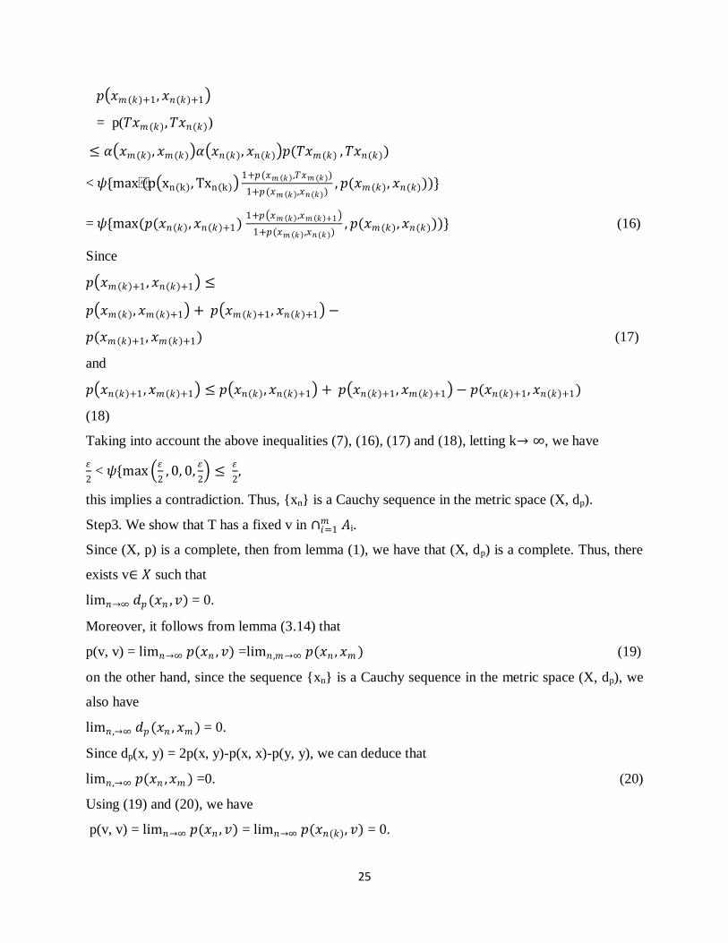
𝑝 𝑥𝑚(𝑘)+1, 𝑥𝑛(𝑘)+1

= p(𝑇𝑥𝑚(𝑘),𝑇𝑥𝑛(𝑘))

≤ 𝛼 𝑥𝑚(𝑘),𝑥𝑚(𝑘) 𝛼 𝑥𝑛(𝑘), 𝑥𝑛(𝑘) 𝑝(𝑇𝑥𝑚(𝑘) ,𝑇𝑥𝑛(𝑘))

< 𝜓{max(p xn k , Txn k 1+𝑝(𝑥𝑚 𝑘 ,𝑇𝑥𝑚 (𝑘))

1+𝑝(𝑥𝑚 𝑘 ,𝑥𝑛(𝑘)), 𝑝(𝑥𝑚(𝑘), 𝑥𝑛(𝑘)))}

= 𝜓{max(𝑝(𝑥𝑛 𝑘 ,𝑥𝑛 𝑘 +1) 1+𝑝 𝑥𝑚 𝑘 ,𝑥𝑚 𝑘 +1

1+𝑝(𝑥𝑚 𝑘 ,𝑥𝑛(𝑘)), 𝑝(𝑥𝑚(𝑘),𝑥𝑛(𝑘)))} (16)

Since

𝑝 𝑥𝑚 𝑘 +1 , 𝑥𝑛 𝑘 +1 ≤

𝑝 𝑥𝑚 𝑘 ,𝑥𝑚 𝑘 +1 + 𝑝 𝑥𝑚 𝑘 +1, 𝑥𝑛 𝑘 +1 −

𝑝(𝑥𝑚 𝑘 +1, 𝑥𝑚 𝑘 +1) (17)

and

𝑝 𝑥𝑛 𝑘 +1 ,𝑥𝑚 𝑘 +1 ≤ 𝑝 𝑥𝑛 𝑘 ,𝑥𝑛 𝑘 +1 + 𝑝 𝑥𝑛 𝑘 +1, 𝑥𝑚 𝑘 +1 − 𝑝(𝑥𝑛 𝑘 +1, 𝑥𝑛 𝑘 +1)

(18)

Taking into account the above inequalities (7), (16), (17) and (18), letting k→ ∞, we have

휀

2 < 𝜓{max

휀

2, 0, 0,

휀

2 ≤

휀

2,

this implies a contradiction. Thus, {xn} is a Cauchy sequence in the metric space (X, dp).

Step3. We show that T has a fixed v in ∩𝑖=1𝑚 𝐴i.

Since (X, p) is a complete, then from lemma (1), we have that (X, dp) is a complete. Thus, there

exists v∈ 𝑋 such that

lim𝑛→∞ 𝑑𝑝(𝑥𝑛 ,𝑣) = 0.

Moreover, it follows from lemma (3.14) that

p(v, v) = lim𝑛→∞ 𝑝(𝑥𝑛 ,𝑣) =lim𝑛 ,𝑚→∞ 𝑝(𝑥𝑛 ,𝑥𝑚 ) (19)

on the other hand, since the sequence {xn} is a Cauchy sequence in the metric space (X, dp), we

also have

lim𝑛 ,→∞ 𝑑𝑝(𝑥𝑛 ,𝑥𝑚 ) = 0.

Since dp(x, y) = 2p(x, y)-p(x, x)-p(y, y), we can deduce that

lim𝑛 ,→∞ 𝑝(𝑥𝑛 ,𝑥𝑚 ) =0. (20)

Using (19) and (20), we have

p(v, v) = lim𝑛→∞ 𝑝(𝑥𝑛 ,𝑣) = lim𝑛→∞ 𝑝(𝑥𝑛(𝑘), 𝑣) = 0.

26

Again by Remark (3.3.2), (p4), and the conditions of the mapping 𝛼, we have

p(xn+1,Tv) = p(Txn, Tv)

≤ 𝛼 𝑥𝑛 ,𝑥𝑛 𝛼 𝑣,𝑣 𝑝(𝑇𝑥𝑛 ,𝑇𝑣)

< 𝜓{max(𝑝 𝑣,𝑇𝑣 1+𝑝 𝑥𝑛 ,𝑇𝑥𝑛

1+𝑝 𝑥𝑛 ,𝑣 , 𝑝 𝑥𝑛 ,𝑣 )}

= 𝜓{max(𝑝 𝑣,𝑇𝑣 1+𝑝 𝑥𝑛 ,𝑥𝑛+1

1+𝑝 𝑥𝑛 ,𝑣 ,𝑝 𝑥𝑛 ,𝑣 )} (21)

Letting n→ ∞ in (21), we get

p(v, Tv) < 𝜓{max 𝑝 𝑣,𝑇𝑣 , 0 } ≤ p(v, Tv),

a contradiction. So, we have p(v, Tv) = 0, that is, Tv = v.

27

BIBLIOGRAPY

1. M. Aamri, D. EI. Moutawakil, Some new common fixed point theorems under strict

contractive conditions, J. Math.Anal.Appl. 27(1)(2002), 181-188.

2. S. Banach, Sur les operations dans les ensembles abstraits et leurs applications aux

equations integral. Fund Math. 3(1922), 133-181.

3. Karapinar, E, Salimi,P :Fixed Point theorems via auxiliary functions. J. Appl. Math.

2012, Article ID 792174(2012).

4. Moradlou, f, Salimi, P, Vetro, P: Some new extensions of Edelstein-Suzuki-type fixed

point theorem of G-metric and G-cone metric spaces. Acta Math. Sci .(In press).

5. M. Abbas, T. Nazir, and S. Romaguera, “Fixed point results for generalized cyclic

contraction mappings in partial metric spaces,” Rev. R. Acad. Cinec. Exactas Fis. Nat.,

Ser. A Mat., RACSAM, vol. 106, no. 1, pp. 287-297, 2012.

6. O. Valero, “On Banach fixed point theorems for partial metric spaces,” Appl. Gen.

Topol., vol. 6, no. 2, pp. 229-240, 2005.s

7. S. G. Matthews, “Partial metric topology,” Dept. of Computer Science, University of

Warwick, Research Report 212, 1992.

8. E. Karapinar and D. M. Erhan, “Fixed point theorems for operators on partial metric

spaces,” Appl. Math. Lett., vol. 24, no. 11, pp. 1894-1899, 2011.

9. 9 Meir, A, Keeler, E: A theorem on contraction mappings. J. Math. Anal. Appl. 28, 326-

329(1969)

10. 10 Aydi, H: Fixed point results for weakly contractive mappings in ordered partial metric

spaces. J. Adv. Math. Stud.4(2), 1-12(2011)