Meir-WinGreen Formula
33
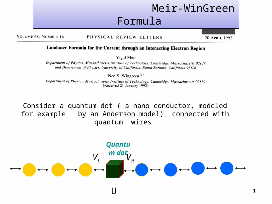
Meir-WinGreen Formula 1 Quantu m dot U L V R V Consider a quantum dot ( a nano conductor, modeled for example by an Anderson model) connected with quantum wires
description
Meir-WinGreen Formula. Quantum dot. U. Consider a quantum dot ( a nano conductor, modeled for example by an Anderson model) connected with quantum wires. Quantum dot. U. - PowerPoint PPT Presentation
Transcript of Meir-WinGreen Formula
Meir-WinGreen Formula Meir-WinGreen Formula
1
Quantum dot
U
LV RV
Consider a quantum dot ( a nano conductor, modeled for example by an Anderson model) connected with quantum wires
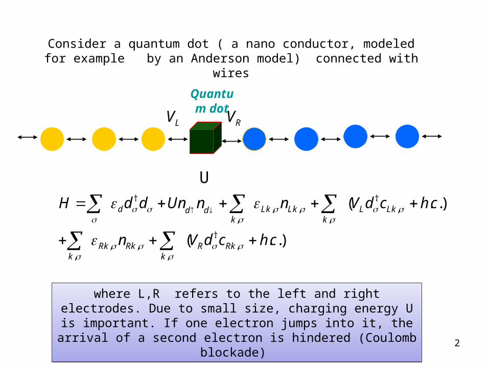
Consider a quantum dot ( a nano conductor, modeled for example by an Anderson model) connected with wires
† †, , ,
, ,
†, , ,
, ,
( . .)
( . .)
d Lk Lk L Lkd dk k
Rk Rk R Rkk k
H d d Un n n V d c h c
n V d c h c
where L,R refers to the left and right electrodes. Due to small size, charging energy U is important. If one electron jumps into it, the arrival of a second electron is hindered (Coulomb blockade)
where L,R refers to the left and right electrodes. Due to small size, charging energy U is important. If one electron jumps into it, the arrival of a second electron is hindered (Coulomb blockade)
2
Quantum dot
U
LV RV
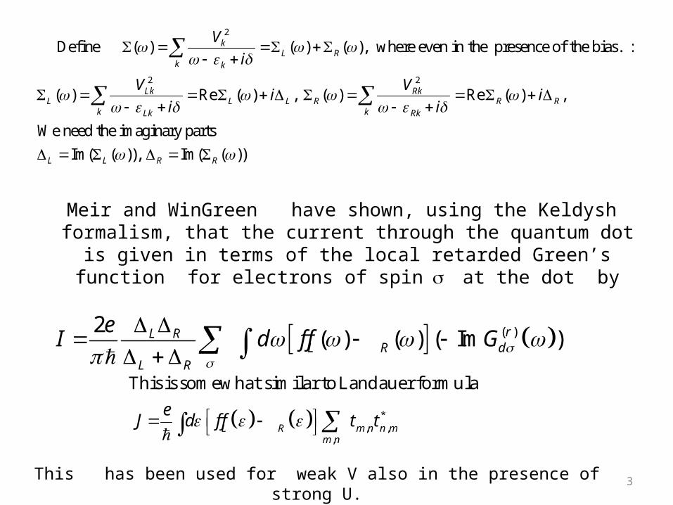
Meir and WinGreen have shown, using the Keldysh formalism, that the current through the quantum dot is given in terms of the local retarded
Green’s function for electrons of spinat the dot by
( )2( ) ( ) ( Im )
rL RL R d
L R
eI d f f G
This has been used for weak V also in the presence of strong U.3
2
2 2
Define ( ) ( ) ( ), where even in the presence of the bias. :
( ) Re ( ) , ( ) Re ( ) ,
We need the imaginary parts
Im( ( )),
kL R
k k
Lk RkL L L R R R
k kLk Rk
L L
V
i
V Vi i
i i
Im( ( )) R R
*
, ,,
Thisissomewhat similartoLandauerformula
L R mn n mmn
eJ d ff t t
44
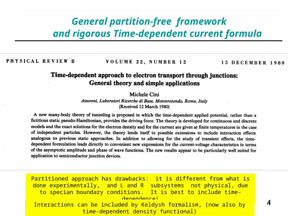
General partition-free framework and rigorous Time-dependent current formula
General partition-free framework and rigorous Time-dependent current formula
Partitioned approach has drawbacks: it is different from what is done experimentally, and L and R subsystems not physical, due to specian
boundary conditions. It is best to include time-dependence!
Interactions can be included by Keldysh formalism, (now also by time-dependent density functional)
55
† †1 1
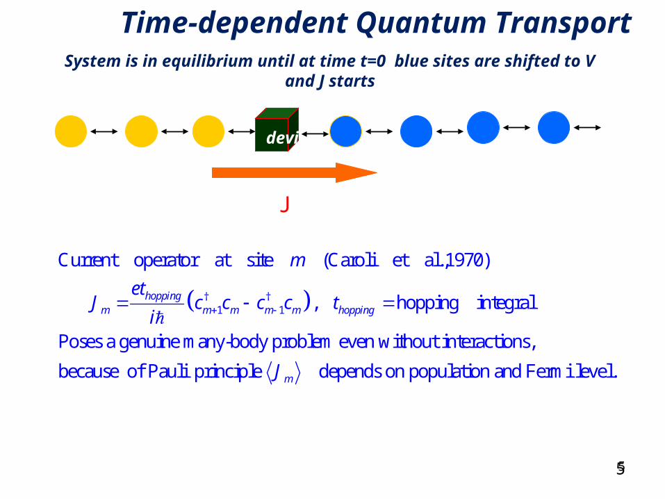
Current operator at site (Caroli et al.,1970)
, hopping integral
Poses a genuine many-body problem even without interactions,
because of Pauli principle depends on
hoppingm m m m m hopping
m
m
etJ c c c c t
i
J
population and Fermi level.
Time-dependent Quantum Transport System is in equilibrium until at time t=0 blue sites are shifted to V and J starts
device
J
6
, 1 , 1' 0
, 1
, 1 , 1
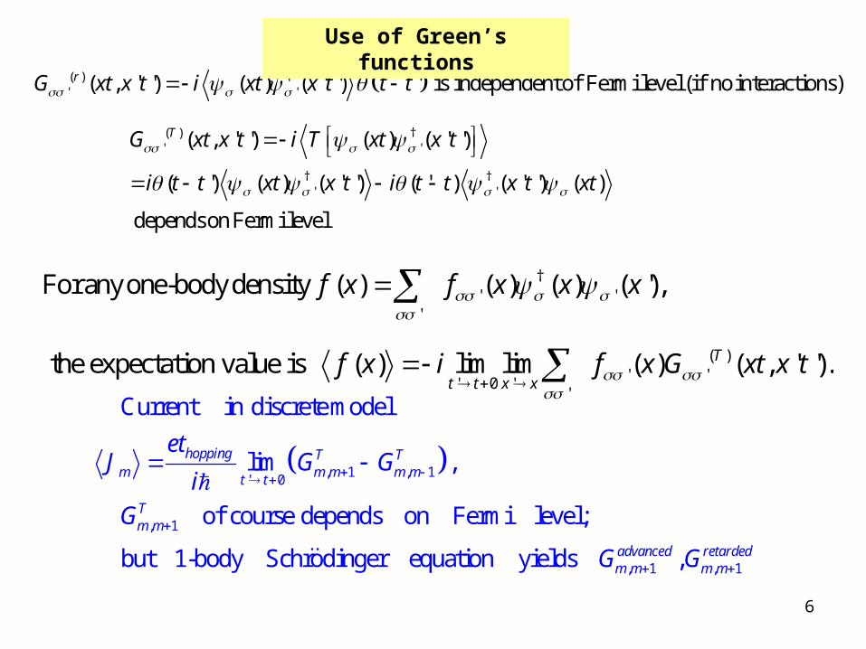
Current in discrete model
lim ,
of course depends on Fermi level;
but 1-body Schrodinger equation yields ,
hopping T Tm m m m m
t t
Tm m
advanced retardedm m m m
etJ G G
i
G
G G
†' '
'
( )' '
' 0 ''
For anyone-bodydensity ( ) ( ) ( ) ( '),
the expectation value is ( ) lim lim ( ) ( , ' ').T
t t x x
f x f x x x
f x i f x G xt x t
( ) †' '
† †' '
( , ' ') ( ) ( ' ')
( ') ( ) ( ' ') ( ' ) ( ' ') ( )
depends on Fermi level
TG xt x t i T xt x t
i t t xt x t i t t x t xt
( ) †' '( , ' ') ( ) ( ' ') ' is independent of Fermi level (if nointeractions)rG xt x t i xt x t t t
Use of Green’s functions
†1 ' '
0
( ) ( ) ( ) i.e. bias is on
eigenstates fo
at time0
r 0,
Fermi function f unbiaor syst ms eed .
q
q
kk k kk
Let H q q
H t V t a a t
V
f
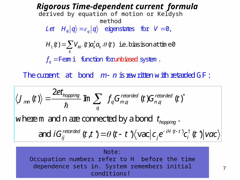
Rigorous Time-dependent current formula
*, ,
( ') †
2( ) Im ( ) ( )
where m and n are connected by a bond .
and ( , ') ( ') vac ( ')
hopping retarded retardedmn q m q n q
q
hopping
retarded iH t tij j i
etJ t f G t G t
t
iG t t t t c e c t vac
7
The current at bond is rewritten with retarded GF : m n
Note:Occupation numbers refer to H before the time dependence sets in.
System remembers initial conditions!
derived by equation of motion or Keldysh method
8
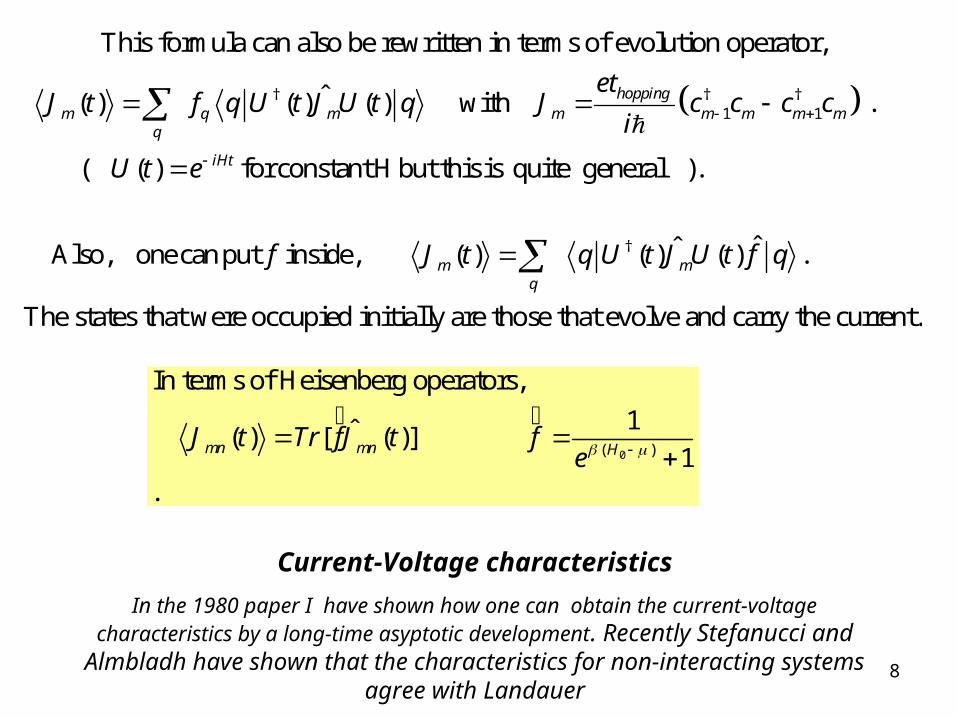
† † †1 1
This formula can also be rewritten in terms of evolution operator,
ˆ ( ) ( ) ( ) with .
( ( ) for constant H but this is quite general ).
Also, onecan put in
hoppingm q m m m m m m
q
iHt
etJ t f q U t J U t q J c c c c
i
U t e
f
† ˆˆside, ( ) ( ) ( ) .
The states that were occupied initially are those that evolve and carry the current.
m mq
J t q U t J U t f q
0( )
In terms of Heisenberg operators,
1ˆ( ) [ ( )]1
.
mn mn HJ t Tr fJ t fe
Current-Voltage characteristics
In the 1980 paper I have shown how one can obtain the current-voltage characteristics by a long-time asyptotic development. Recently Stefanucci and Almbladh have shown that
the characteristics for non-interacting systems agree with Landauer
9
2 2
0
22
2
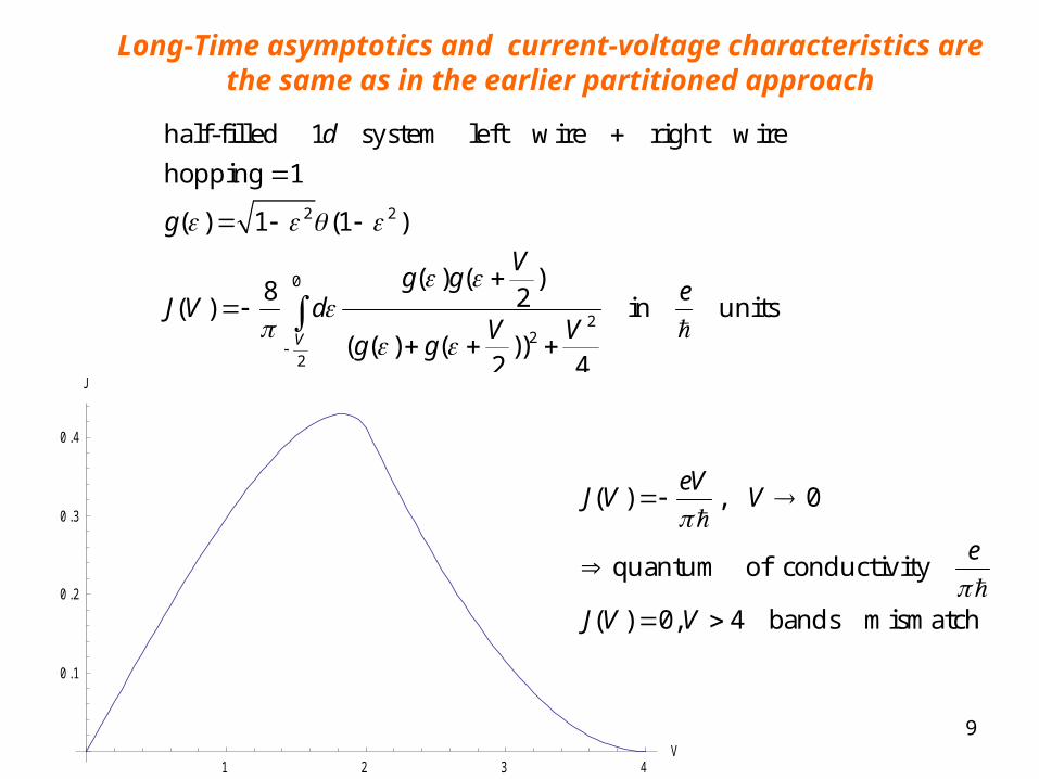
half-filled 1 system left wire right wire
hopping 1
( ) 1 (1 )
( ) ( )8 2( ) in units( ( ) ( ))
2 4V
d
g
Vg g e
J V dV V
g g
1 2 3 4V
0 .1
0 .2
0 .3
0 .4
J
( ) , 0
quantum of conductivity
( ) 0, 4 bands mismatch
eVJ V V
e
J V V
Long-Time asymptotics and current-voltage characteristics are the same as in the earlier partitioned approach
10
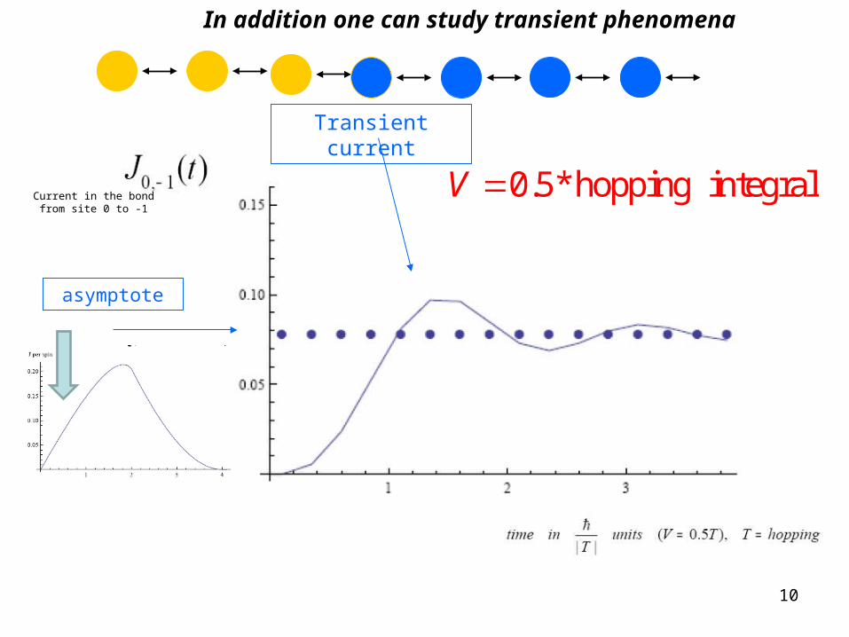
Current in the bond from site 0 to -1
Transient current
asymptote
0.5*hopping integralV
In addition one can study transient phenomena
M. Cini E.Perfetto C. Ciccarelli G. Stefanucci and S. Bellucci, PHYSICAL REVIEW B 80, 125427 2009
1
0
( ) ( ) ,
0, t<0 ( )
0.5, t>0
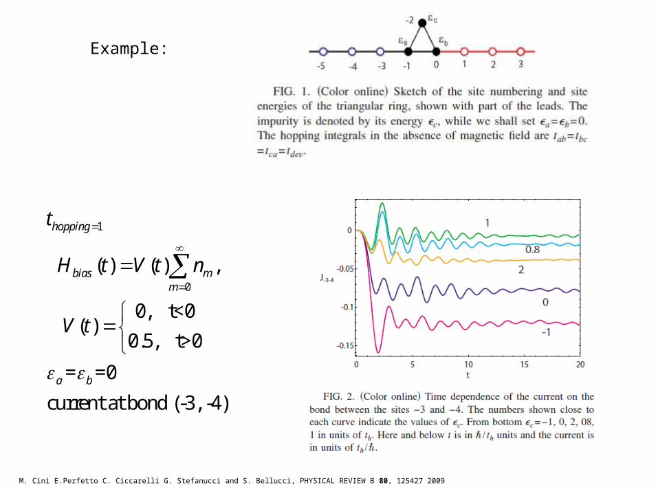
= =0
current at bond (-3, -4)
hopping
bias mm
a b
t
H t V t n
V t
Example:
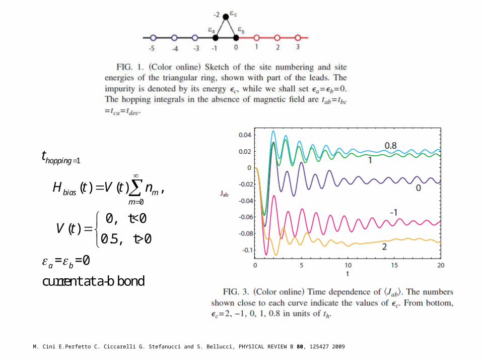
M. Cini E.Perfetto C. Ciccarelli G. Stefanucci and S. Bellucci, PHYSICAL REVIEW B 80, 125427 2009
1
0
( ) ( ) ,
0, t<0 ( )
0.5, t>0
= =0
current at a-b bond
hopping
bias mm
a b
t
H t V t n
V t
13
G. Stefanucci and C.O. Almbladh (Phys. Rev 2004) extended to TDDFT LDA scheme
TDDFT LDA scheme not enough for hard correlation effects: Josephson effect would not arise
Keldysh diagrams should allow extension to interacting systems, but this is largely unexplored.
Retardation + relativistic effects totally to be invented!
14
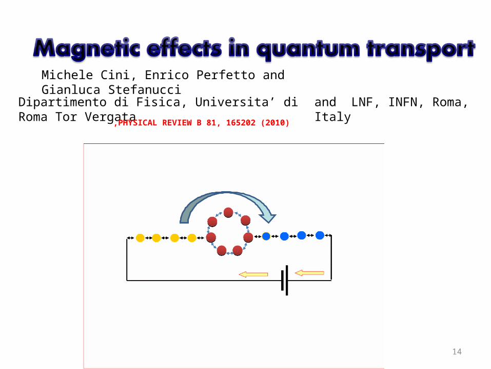
Michele Cini, Enrico Perfetto and Gianluca Stefanucci
Dipartimento di Fisica, Universita’ di Roma Tor Vergata and LNF, INFN, Roma, Italy
,PHYSICAL REVIEW B 81, 165202 (2010)
1515
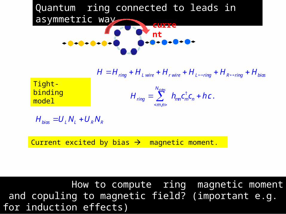
ring L wire r wire L ring R ring biasH H H H H H H
Tight-binding model †
,
. .sidesN
ring mn m nm n
H h c c h c
How to compute ring magnetic moment and copuling to magnetic field? (important e.g. for induction effects)
Current excited by bias magnetic moment.
bias L L R RH U N U N
Quantum ring connected to leads in asymmetric way
current
1616
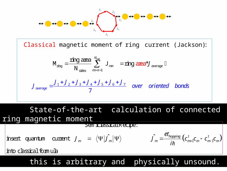
State-of-the-art calculation of connected ring magnetic moment
† †1 1
Semiclassical Recipe:
ˆ ˆinsert quantum current hoppingm m m m m m m
etJ J J c c c c
i
into classical formula
magnetic moment of ring current Classi (Jackscal on):
ring1sides
ring areaaring *
Nrea
latiN
mn averagem n
J
M J
1 2 3 4 5 6 7
7
average
J J J J J J JJ over oriented bonds
J1 J2
J3
J4
J5
J7
J6
this is arbitrary and physically unsound.
17
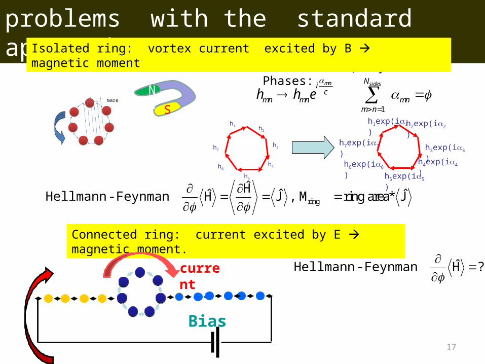
problems with the standard approach
Insert flux by Peierls Phases:
1
mn sidesN
ic
mn mn mnm n
h h eNN S
ring
ˆˆ ˆ ˆ, ring area*
HHellmann-Feynman H J M J
Isolated ring: vortex current excited by B magnetic moment
Connected ring: current excited by E magnetic moment.
Bias
current
h1 h2
h3
h4
h5
h7
h6
h5exp(i5)
h6exp(i6)
h1exp(i1) h2exp(i2)
h4exp(i4)
h3exp(i3)h7exp(i7)
ˆ ?
Hellmann-Feynman H

18
c
a b
Insert flux by Peierls Phases:
1
mn sidesN
ic
mn mn mnm n
h h e
NN S
ac ab bac b H J
00 0
0 bc
ab
0 ac
All real orbitals, all hoppings=
Gauges
Blue orbital picks phase , previous bond e i, following bond e-i
Physics does not change
ie ie
Probe flux, vanishes eventually
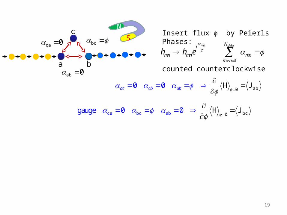
19
c
a b
Insert flux by Peierls Phases:
1
mn sidesN
ic
mn mn mnm n
h h e
NN S
00 0
abH Jac cb ab
bc ca 0
0 ab
0gauge 0 0
ca bc a bb cH J
counted counterclockwise
2020
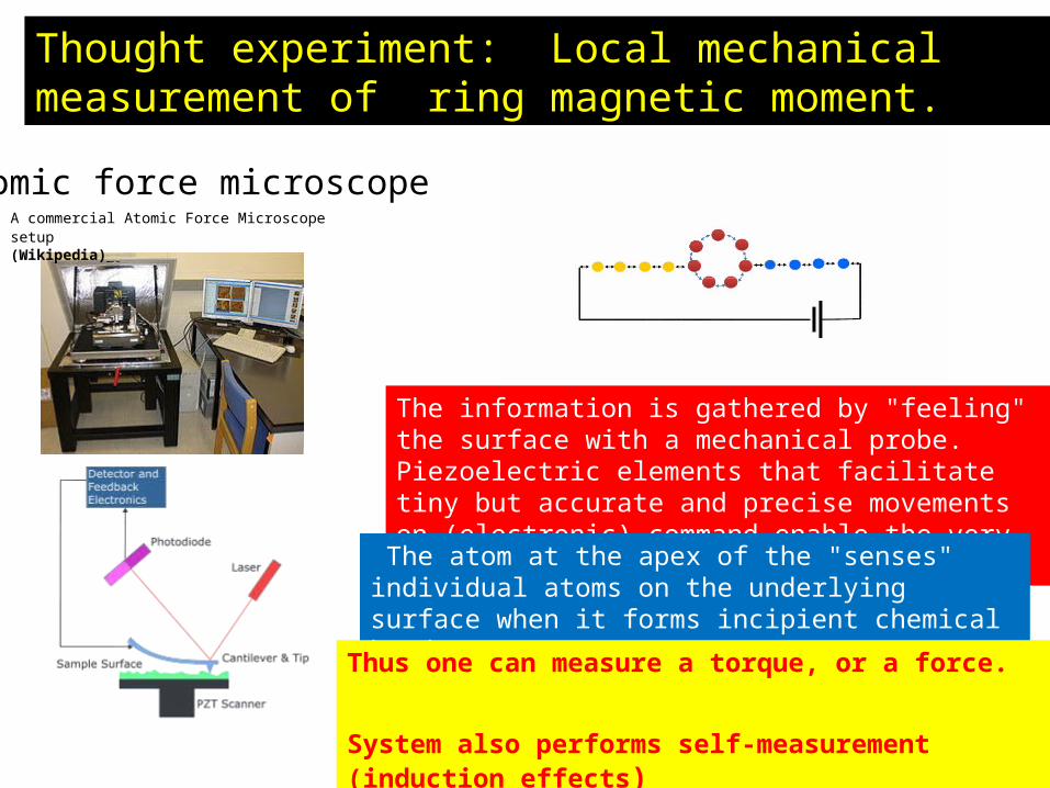
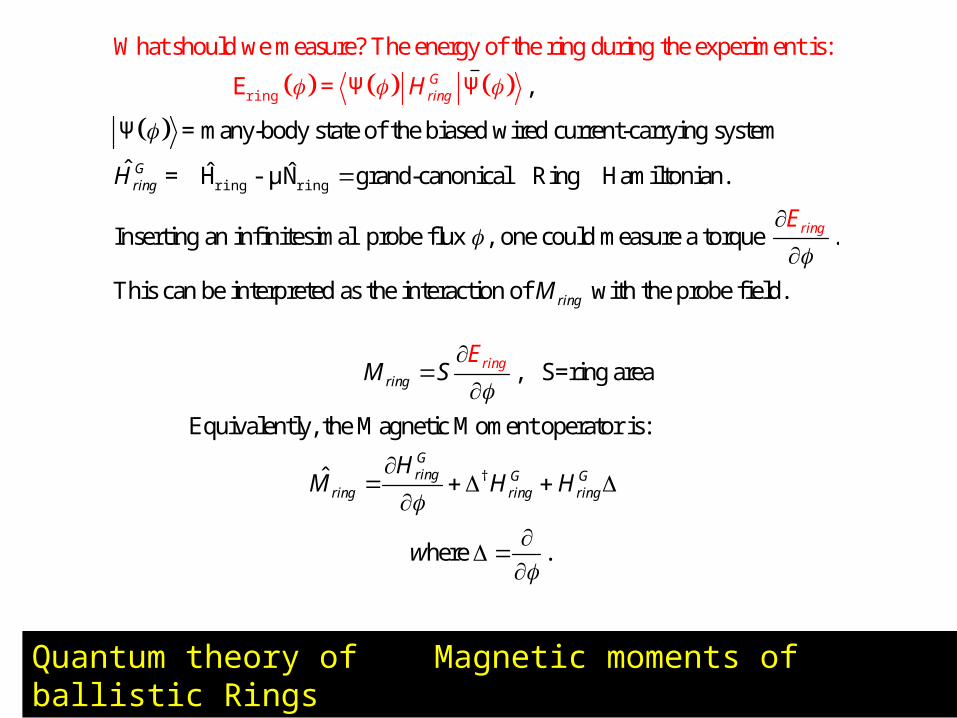
Thought experiment: Local mechanical measurement of ring magnetic moment.
The information is gathered by "feeling" the surface with a mechanical probe. Piezoelectric elements that facilitate tiny but accurate and precise movements on (electronic) command enable the very precise scanning.
The atom at the apex of the "senses" individual atoms on the underlying surface when it forms incipient chemical bonds.
Atomic force microscopeA commercial Atomic Force Microscope setup (Wikipedia)
Thus one can measure a torque, or a force.
System also performs self-measurement (induction effects)
2121
†
, S=ring area
Equivalently, the Magnetic Moment operator is:
ˆ
here .
ring
Gring G G
ring ring rin
n
g
ri gM S
HM
E
H H
w
,
= many-body state
What should we meas
of the biased wire
ure? The energy of the ring during the
d current-carrying system
ˆ ˆ ˆ grand-canonic
experim
al Ring Ha
ent is:
mGr
Gring
ing
H
H
ring ri
in
ng
r g
Ψ
= H
= Ψ
- N
Ψ
μ
E
iltonian.
Inserting an infinitesimal probe flux , one could measure a torque .
This can be interpreted as the interaction of with the probe field.
r
ring
ing
M
E
Quantum theory of Magnetic moments of ballistic Rings
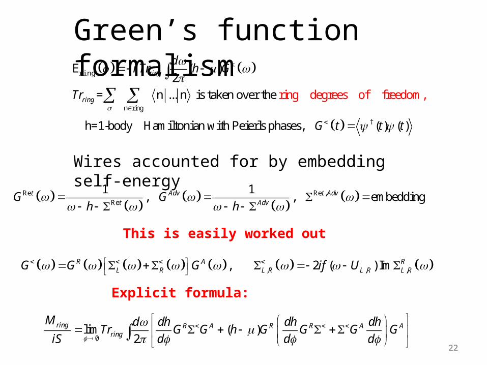
2222
n ring
†
ring degrees of
( )2
= n ... n is taken over the
h=1-body Hamiltonian with Peierls phases,
freedom,
( ) ( )
ring
ring
di Tr h G
Tr
G t t t
ringE
0lim ( )
2
ring R A R R A A
ring
M d dh dh dhTr G G h G G G G
iS d d d
Re Re ,Re
1 1, , embeddingt Adv t Adv
t AdvG G
h h
, , ,, 2 ( ) Im R A R
L R L R L R L RG G G if U
Wires accounted for by embedding self-energy
Green’s function formalism
Explicit formula:
This is easily worked out
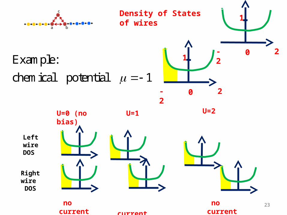
2323
2-2 0
1Density of States of wires
Example:
chemical potential 1 2-2 0
1
U=0 (no bias)
no current
Left wire DOS
Right wire DOS
U=1
current no current
U=2
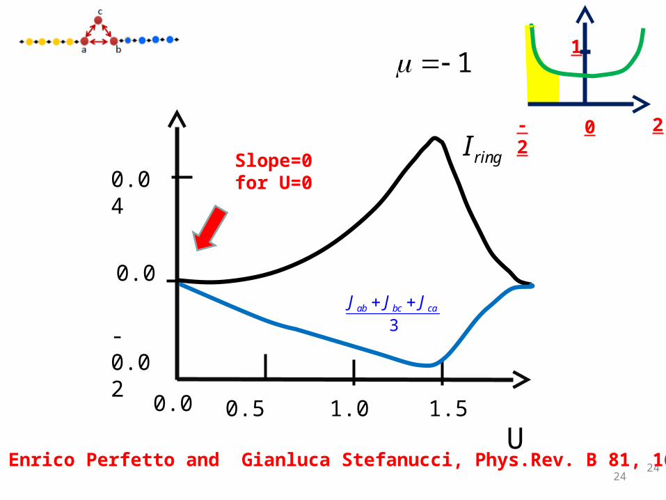
2424
U1.00.0 0.5 1.5
0.04
0.0
-0.02
ringI
3
ab bc caJ J J
1
2-2 0
1
Slope=0 for U=0
Cini Michele, Enrico Perfetto and Gianluca Stefanucci, Phys.Rev. B 81, 165202-1 (2010)
2525
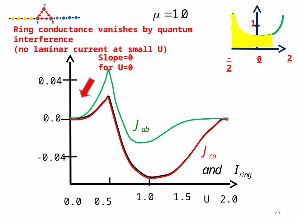
1.0
0.04
-0.04
0.0
0.0 0.5 1.0 1.5 2.0U
abJ
i
ca
r ngand I
J
2-2 0
1Ring conductance vanishes by quantum interference(no laminar current at small U)
Slope=0 for U=0
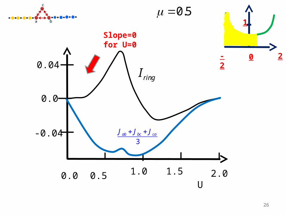
2626
0.0 0.5 1.0 1.5 2.0U
-0.04
0.04
0.0
ringI
3
ab bc caJ J J
0.5
2-2 0
1
Slope=0 for U=0
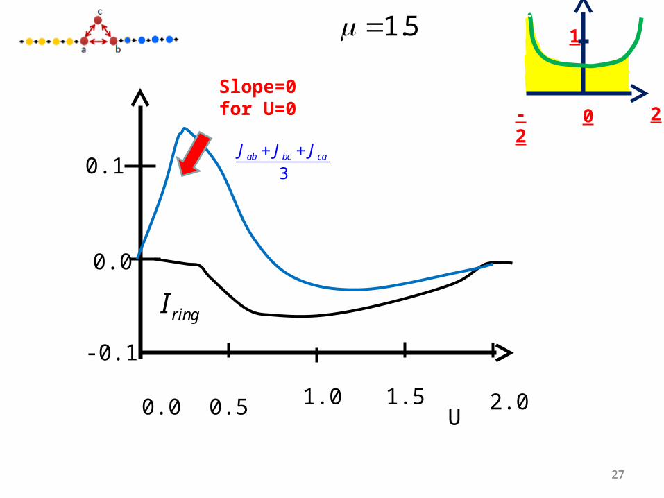
2727
1.5
0.0 0.5 1.0 1.5 2.0U
-0.1
0.1
0.0
ringI
3
ab bc caJ J J
2-2 0
1
Slope=0 for U=0
28
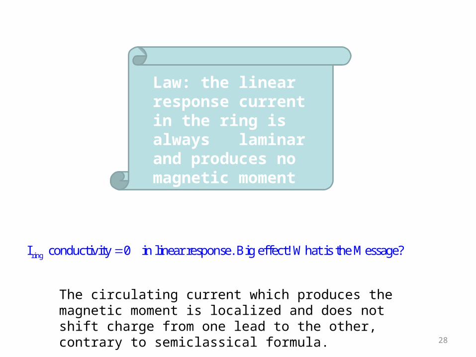
Law: the linear response current in the ring is always laminar and produces no magnetic moment
ringI conductivity 0 in linear response. Big effect! What is the Message?
The circulating current which produces the magnetic moment is localized and does not shift charge from one lead to the other, contrary to semiclassical formula.
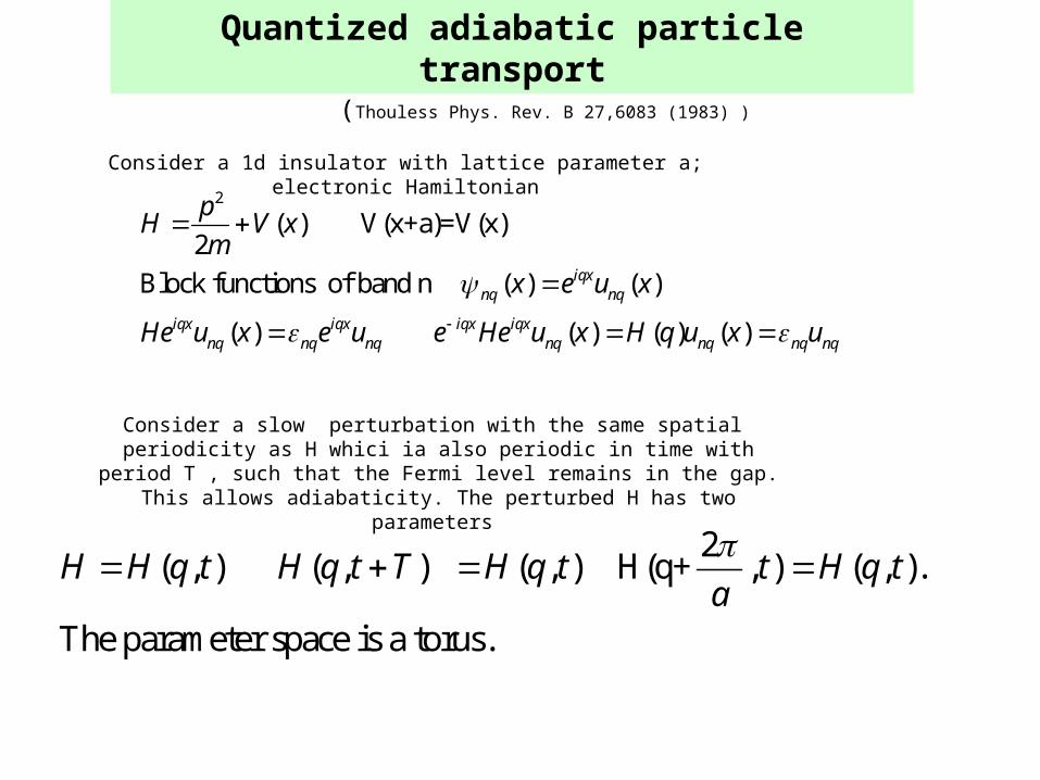
Quantized adiabatic particle transport
(Thouless Phys. Rev. B 27,6083 (1983) )
Consider a 1d insulator with lattice parameter a; electronic Hamiltonian
2
( ) V(x+a)=V(x) 2
Block functions of band n ( ) ( )
( ) ( ) ( ) ( )
iqxnq nq
iqx iqx iqx iqxnq nq nq nq nq nq nq
pH V x
m
x e u x
He u x e u e He u x H q u x u
Consider a slow perturbation with the same spatial periodicity as H whici ia also periodic in time with period T , such that the Fermi level remains in the gap. This allows adiabaticity. The perturbed H
has two parameters
2( , ) ( , ) ( , ) H(q+ , ) ( , ).
The parameter space is a torus.
H H q t H q t T H q t t H q ta
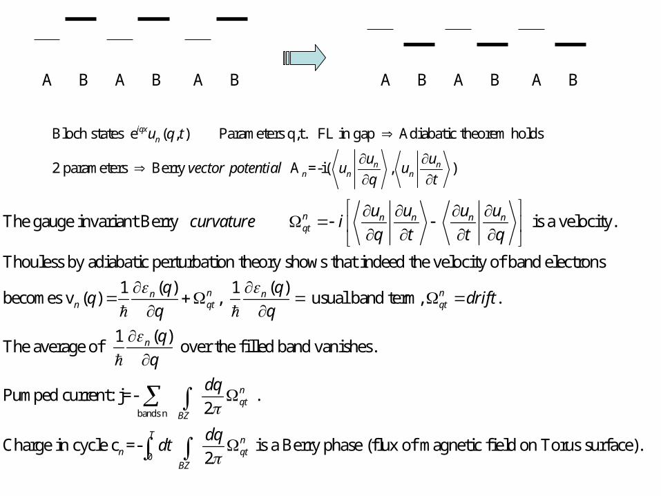
Bloch states e ( , ) Parameters q,t. FL in gap Adiabatic theorem holds
2 parameters Berry A =-i( , )
iqxn
n nn n n
u q t
u uvector potential u u
q t
A B A B A B A B A B A B
The gauge invariant Berry is a velocity.
Thouless by adiabatic perturbation theory shows that indeed the velocity of band electrons
1becomes v ( )
n n n n nqt
n
u u u ucurvature i
q t t q
q
bands n
0
( ) ( )1, usual band term, .
( )1The average of over the filled band vanishes.
Pumped current: j=- .2
Charge in cycle c =- is a Berry2
n nn nqt qt
n
nqt
BZ
T nn qt
BZ
q qdrift
q q
q
q
dq
dqdt
phase (flux of magnetic field on Torus surface).
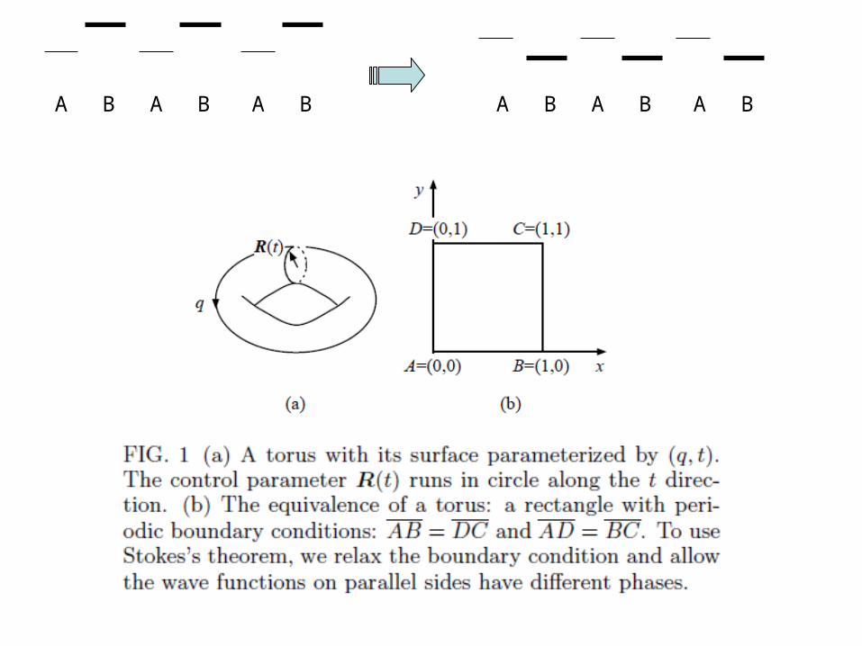
A B A B A B A B A B A B
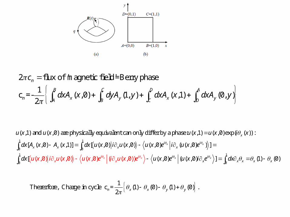
2 flux of 'magnetic field'=Berry phase
1c =- ( ,0) (1, ) ( ,1) (0, )
2
n
B C D A
n x y x yA B C D
c
dxA x dyA y dxA x dxA y
1 1
0 0
1
0( ,0) ( ,0) (
( ,1) and ( ,0) are physically equivalent can only differ by a phase: ( ,1) ( ,0)exp( ( )) :
[ ( ,0) ( ,1)] [ ( ,0) ( ,0) ( ,0) ( ( ,0) ) ]
[ ,0)
x
x
x
x
i ix x x x
ix
u x u x u x u x i x
dx A x A x dx u x i u x u x e i u x e
d u x i u x u x ex
1
0( ,0) ( ( ,0( ( ) ],0 () )) 1 (0)xx xi i
x x x x xi
x u x e u x i e xi u x e d
1Thererfore, Charge in cycle c = (1) (0) (1) (0) .
2n x x y y
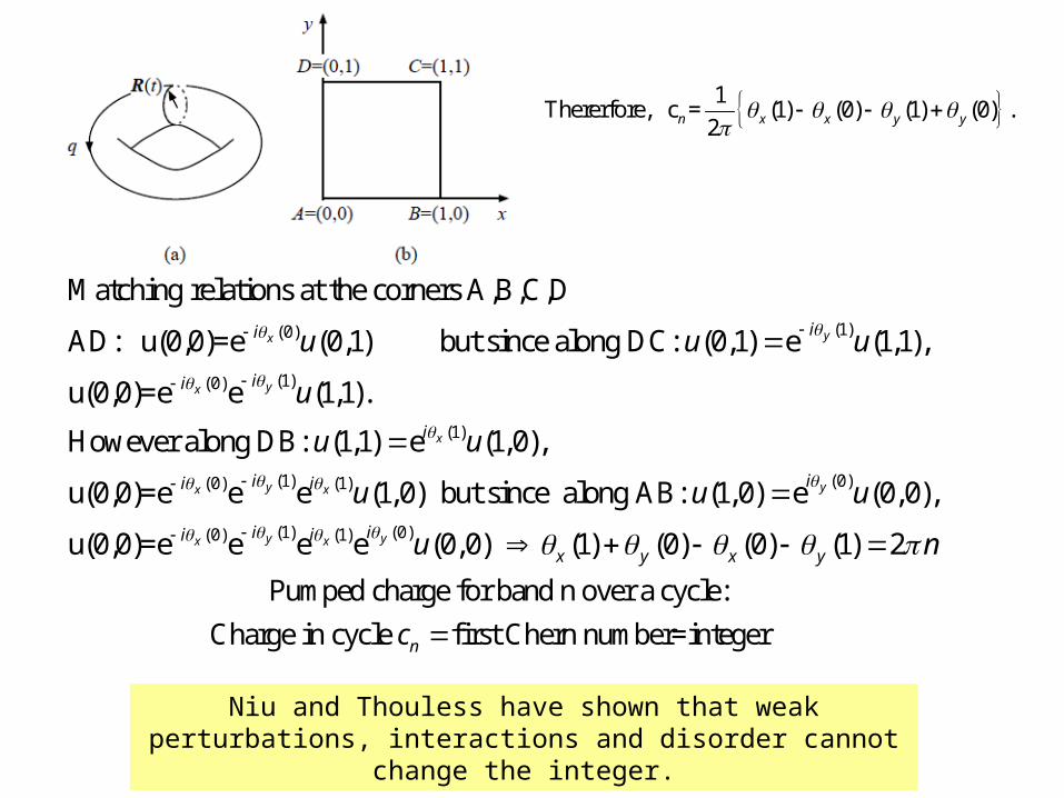
Pumped charge for band n over a cycle:
Charge in cycle first Chern number=integer nc
Niu and Thouless have shown that weak perturbations, interactions and disorder cannot change the integer.
1Thererfore, c = (1) (0) (1) (0) .
2n x x y y
(1)(0)
(1)(0)
(1)
Matching relations at the corners A,B,C,D
AD: u(0,0)=e (0,1) but since along DC: (0,1) e (1,1),
u(0,0)=e e (1,1).
However along DB: (1,1) e (1,0),
u(0,0)=e
yx
yx
x
x
ii
ii
i
i
u u u
u
u u
(1) (0)(0) (1)
(1) (0)(0) (1)
e e (1,0) but since along AB: (1,0) e (0,0),
u(0,0)=e e e e (0,0) (1) (0) (0) (1) 2
y yx
y yx x
i ii
i ii ix y x y
u u u
u n


![ElEleecctrontron--vvibibrarationtion ssccaatteritteringng ... · Current (Meir-Wingreen) TThhee DFDFTTBB aapppprrooaacchh DFTB = DFT based Tight-Binding method 0 [ ] [ ] rep k k k](https://static.fdocuments.net/doc/165x107/5e2116986214331e050a7d56/eleleecctrontron-vvibibrarationtion-ssccaatteritteringng-current-meir-wingreen.jpg)