Exact Analysis of a Common-Source MOSFET Amplifier

Consider the common-source MOSFET amplifier driven from signal source vs

with Thévenin equivalent resistance RS and a load consisting of a parallel resistor RL and capacitor CL as shown below:

VDD

RL

CL

M1

vS

RS

iS

vout +

_

+

_

Calculate the voltage gain, AV (= vout/vs), for this amplifier.

1

2

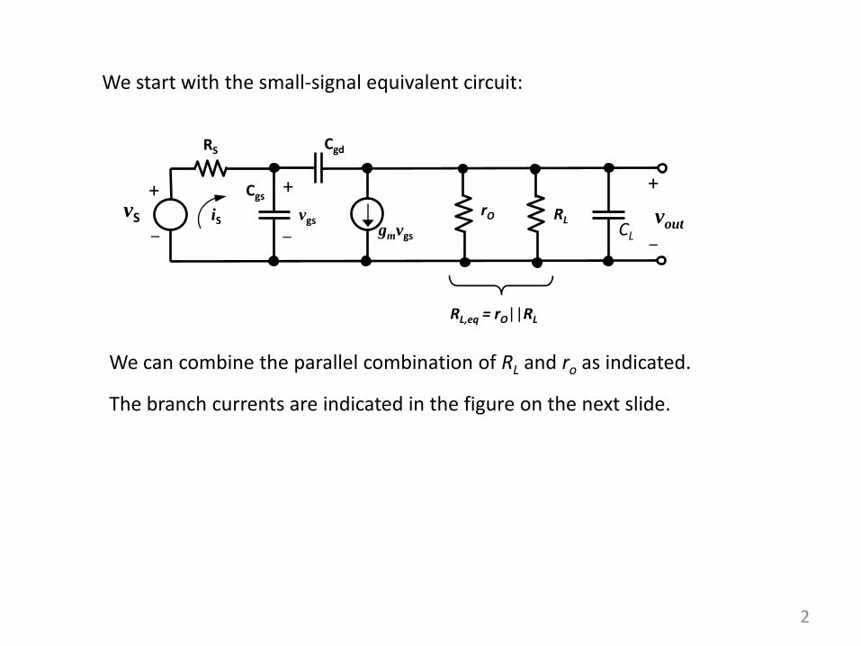
We start with the small-signal equivalent circuit:

CL

vS

RS

iS vgs

+

_

+

_

Cgs

Cgd

gmvgs

rO RL

_

+

vout

RL,eq = rO||RL

We can combine the parallel combination of RL and ro as indicated.

The branch currents are indicated in the figure on the next slide.

3

vS

RS

iS

+

_

Cgs

Cgd

CL

vgs

+

_

gmvgs

_

+

vout rO||RL

sCgsvgs

sCgd(vgs – vout)

rO||RL

vout sCLvout

iS

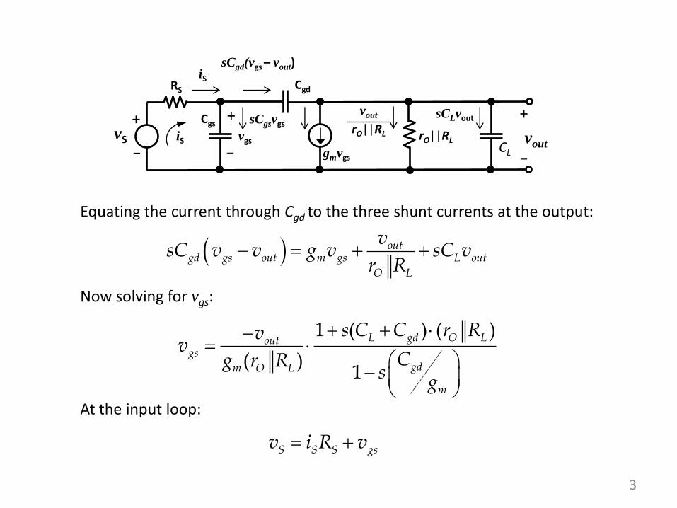
Equating the current through Cgd to the three shunt currents at the output:

outgd gs out m gs L out

O L

vsC v v g v sC v

r R

Now solving for vgs:

1 ( ) ( )

( )1

L gd O Loutgs

gdm O L

m

s C C r Rvv

Cg r Rs

g

At the input loop:

S S S gsv i R v

4

vS

RS

iS

+

_

Cgs

Cgd

CL

vgs

+

_

gmvgs

_

+

vout rO||RL

sCgsvgs

sCgd(vgs – vout)

rO||RL

vout sCLvout

iS

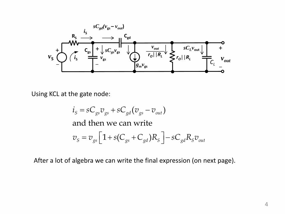
Using KCL at the gate node:

( )

and then we can write

1 ( )

S gs gs gd gs out

S gs gs gd S gd S out

i sC v sC v v

v v s C C R sC R v

After a lot of algebra we can write the final expression (on next page).

5

2

( ) 1

1 (1 ( )) ( ) ( )

( ) ( )

gd

m O L

mout

S gs gd m O L S gd L O L

gd L gs L gd S O L

Cg r R s

gv

v s C C g r R R C C r R

s C C C C C R r R

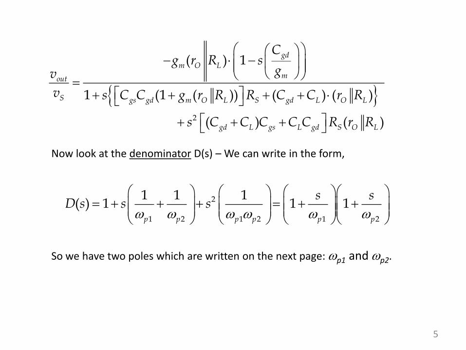
Now look at the denominator D(s) – We can write in the form,

2

1 2 1 2 1 2

1 1 1( ) 1 1 1

p p p p p p

s sD s s s

So we have two poles which are written on the next page: p1 and p2.

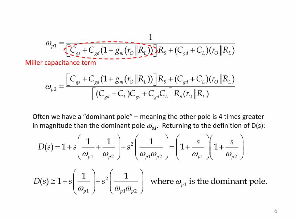
6

1

1

(1 ( )) ( )( )p

gs gd m O L S gd L O LC C g r R R C C r R

2

(1 ( )) ( )( )

( ) ( )

gs gd m O L S gd L O L

p

gd L gs gd L S O L

C C g r R R C C r R

C C C C C R r R

2

1 2 1 2 1 2

1 1 1( ) 1 1 1

p p p p p p

s sD s s s

Often we have a “dominant pole” – meaning the other pole is 4 times greater in magnitude than the dominant pole p1. Returning to the definition of D(s):

21

1 1 2

1 1( ) 1 where is the dominant pole.p

p p p

D s s s

Miller capacitance term

7

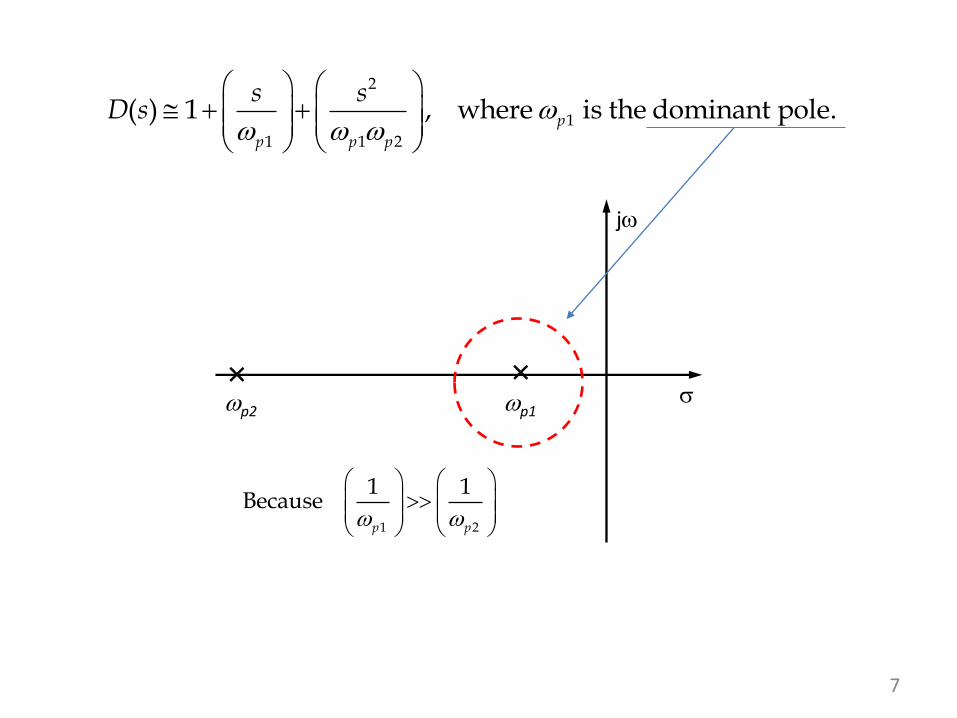
2

1

1 1 2

( ) 1 , where is the dominant pole.p

p p p

s sD s

j

p1 p2

1 2

1 1Because

p p

8

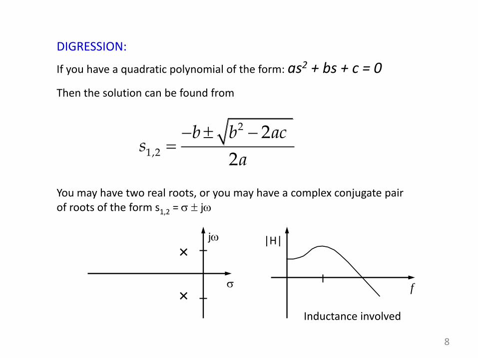
If you have a quadratic polynomial of the form: as2 + bs + c = 0

Then the solution can be found from

2

1,2

2

2

b b acs

a

You may have two real roots, or you may have a complex conjugate pair of roots of the form s1,2 = j

j

DIGRESSION:

f

|H|

Inductance involved

9

Miller’s Theorem (from Razavi)

• If Av is the voltage gain from node 1 to 2, then a floating impedance ZF can be converted to two grounded impedances Z1 and Z2:

v

FF

F AZ

VV

VZZ

Z

V

Z

VV

1

1

21

11

1

121

1 2 2 22

2 1 2

1

11

F F

F

v

V V V VZ Z Z

Z Z V VA

10

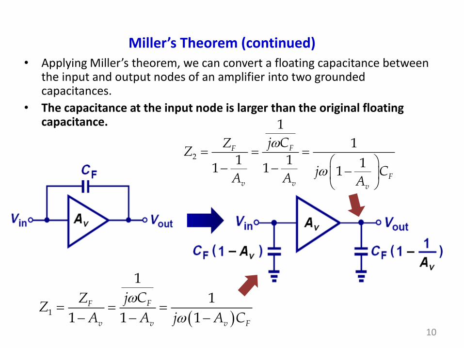
• Applying Miller’s theorem, we can convert a floating capacitance between the input and output nodes of an amplifier into two grounded capacitances.

• The capacitance at the input node is larger than the original floating capacitance.

1

1

1

1 1 1FF

v v v F

j CZZ

A A j A C

2

1

1

1 1 11 1 1

FF

Fv v v

j CZZ

j CA A A

Miller’s Theorem (continued)

11

(1 ( )) (1 )in F m D F m DC C g R C g R

Miller’s Theorem

0

0

0

gs

gd

C

C

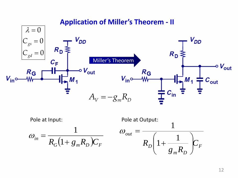
Application of Miller’s Theorem - I

Capacitor Cin is given by

V m DA g R

Capacitor Cout is given by

1 11 1out F F

m D m D

C C Cg R g R

12

Miller’s Theorem

0

0

0

gs

gd

C

C

Application of Miller’s Theorem - II

V m DA g R

FDmG

inCRgR

1

1

F

Dm

D

out

CRg

R

1

1

1

Pole at Input: Pole at Output:

13

CL

vS

RS

iS vgs

+

_

+

_

Cgs

Cgd

gmvgs

rO RL

_

+

vout

RL,eq = rO||RL

Back to our common-source MOSFET amplifier

What is the midband voltage gain AV?

Set all capacitors to open circuits for midband voltage gain calculation.

vS

RS

vgs

+

_ _

gmvgs

rO RL

_

+

vout

RL,eq = rO||RL

+

( )V m O LA g r R

14

Cout

vS

RS

iS vgs

+

_

+

_

Cin

gmvgs

_

+ vout rO||RL

1 (in gs gd m O LC C C g r R

Applying Miller’s Theorem to CS MOSFET Amplifier

11

(out L gd

m O L

C C Cg r R

Now we have only an input loop and an output loop to deal with. This means we will have an input pole and an output pole to contend with.

15

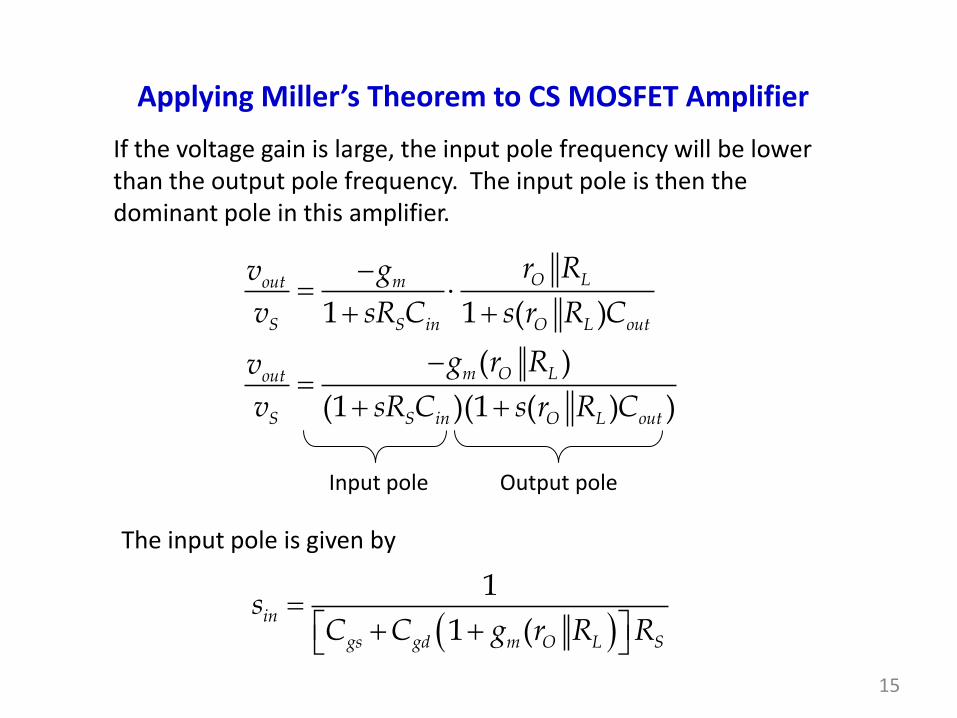
Applying Miller’s Theorem to CS MOSFET Amplifier

If the voltage gain is large, the input pole frequency will be lower than the output pole frequency. The input pole is then the dominant pole in this amplifier.

1 1 ( )

( )

(1 )(1 ( ) )

O Lmout

S S in O L out

m O Lout

S S in O L out

r Rgv

v sR C s r R C

g r Rv

v sR C s r R C

Input pole Output pole

The input pole is given by

1

1 (in

gs gd m O L S

sC C g r R R

16

Comparing dominant pole terms from “exact analysis” to that from Miller’s Theorem

1

1

1 (in p

gs gd m O L S

sC C g r R R

1

1

(1 ( )) ( )( )p

gs gd m O L S gd L O LC C g r R R C C r R

From our “exact analysis”:

From our analysis using Miller’s theorem:

17

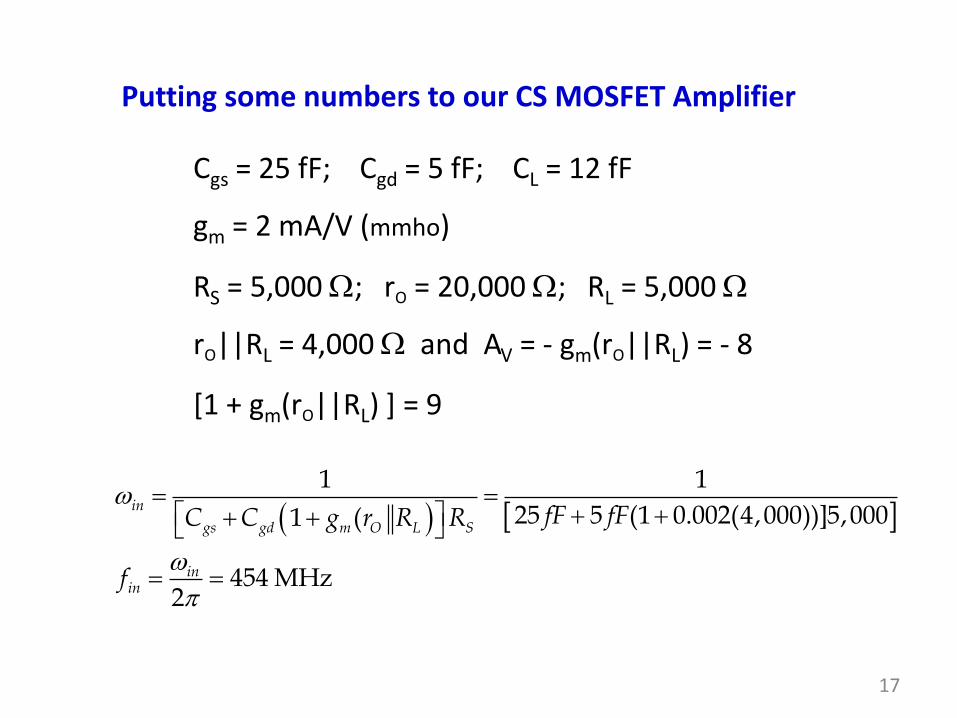
Putting some numbers to our CS MOSFET Amplifier

Cgs = 25 fF; Cgd = 5 fF; CL = 12 fF

gm = 2 mA/V (mmho)

RS = 5,000 ; rO = 20,000 ; RL = 5,000

rO||RL = 4,000 and AV = - gm(rO||RL) = - 8

[1 + gm(rO||RL) ] = 9

1 1

25 5 (1 0.002(4,000))]5,0001 (

454 MHz2

in

gs gd m O L S

inin

fF fFC C g r R R

f

18

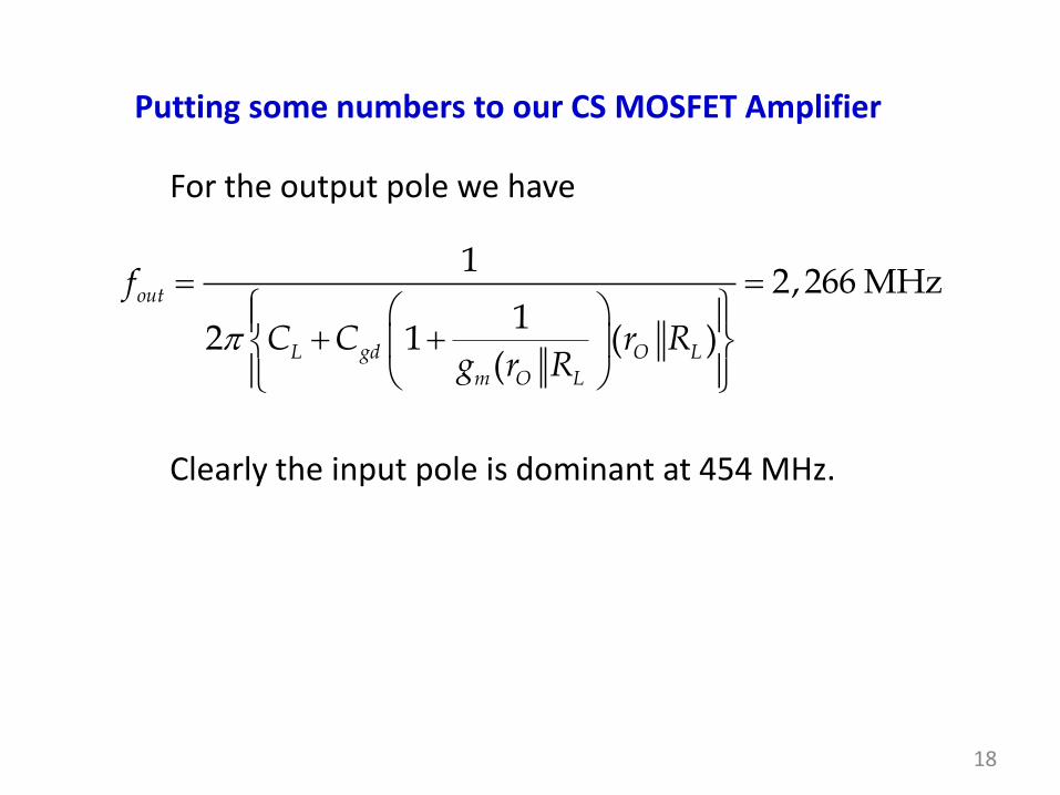
Putting some numbers to our CS MOSFET Amplifier

For the output pole we have

12,266 MHz

12 1 ( )

(

out

L gd O L

m O L

f

C C r Rg r R

Clearly the input pole is dominant at 454 MHz.

19

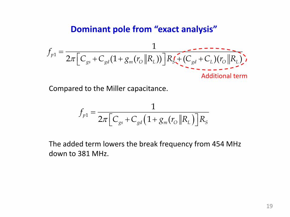
1

1

2 (1 ( )) ( )( )p

gs gd m O L S gd L O L

fC C g r R R C C r R

Dominant pole from “exact analysis”

Compared to the Miller capacitance.

1

1

2 1 (p

gs gd m O L S

fC C g r R R

Additional term

The added term lowers the break frequency from 454 MHz down to 381 MHz.

20

NEXT: Open-Circuit Time Constant Analysis

21 2

21 2

1( )

1

mm

nn

a s a s a sH s K

b s b s b s

When the poles and zeros are easily found, then it is relatively easy to determine the dominant pole. But often it is not easy to determine the dominant pole. The coefficient b1 is especially important because

1

1 2 3

1 1 1 1

p p p pn

b

How do we determine the pi values? We will consider all capacitors in the overall circuit one at a time.

21

Open-Circuit Time Constant Analysis

We consider each capacitor in the overall circuit one at a time by setting every other small capacitor to an open circuit and letting independent voltage sources be short circuits. The value of b1 is computed by summing the individual time constants, called “open-circuit time constants.” and

11

n

io ii

b R C

1

1

1 1H n

io ii

bR C

Time constant = RC

22

Open-Circuit Time Constant Rules

• For each “small” capacitor in the circuit:

– Open-circuit all other “small” capacitors

– Short circuit all “big” capacitors

– Turn off all independent sources

– Replace cap under question with current or voltage source

– Find equivalent input impedance seen by capacitor

– Form RC time constant

• This procedure is best illustrated with an example…