
Estimating Crystallite Size Using XRD - Welcome to Prism...
105
Estimating Crystallite Size Estimating Crystallite Size Estimating Crystallite Size Estimating Crystallite Size Using XRD Using XRD Using XRD Using XRD Scott A Speakman, Ph.D. 13-4009A [email protected] http://prism.mit.edu/xray MIT Center for Materials Science and Engineering
Transcript of Estimating Crystallite Size Using XRD - Welcome to Prism...
Estimating Crystallite SizeEstimating Crystallite SizeEstimating Crystallite SizeEstimating Crystallite SizeUsing XRDUsing XRDUsing XRDUsing XRD
Scott A Speakman, Ph.D.13-4009A
http://prism.mit.edu/xray
MIT Center for Materials Science and Engineering
Center for Materials Science and Engineeringhttp://prism.mit.edu/xray
Warning
• These slides have not been extensively proof-read, and therefore may contain errors.
• While I have tried to cite all references, I may have missed some– these slides were prepared for an informal lecture and not for publication.
• If you note a mistake or a missing citation, please let me know and I will correct it.
• I hope to add commentary in the notes section of these slides, offering additional details. However, these notes are incomplete so far.
Center for Materials Science and Engineeringhttp://prism.mit.edu/xray
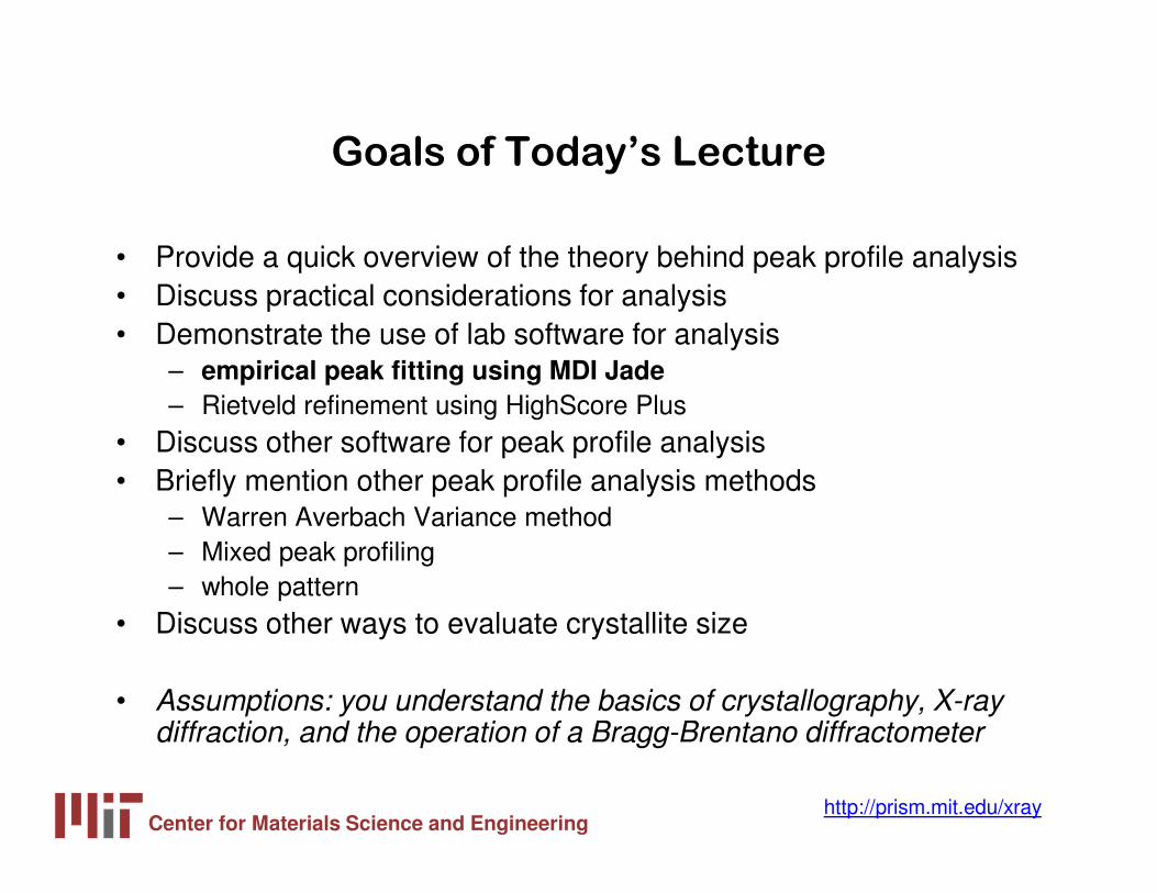
Goals of Today’s Lecture
• Provide a quick overview of the theory behind peak profile analysis• Discuss practical considerations for analysis• Demonstrate the use of lab software for analysis
– empirical peak fitting using MDI Jade– Rietveld refinement using HighScore Plus
• Discuss other software for peak profile analysis• Briefly mention other peak profile analysis methods
– Warren Averbach Variance method– Mixed peak profiling– whole pattern
• Discuss other ways to evaluate crystallite size
• Assumptions: you understand the basics of crystallography, X-ray diffraction, and the operation of a Bragg-Brentano diffractometer
Center for Materials Science and Engineeringhttp://prism.mit.edu/xray
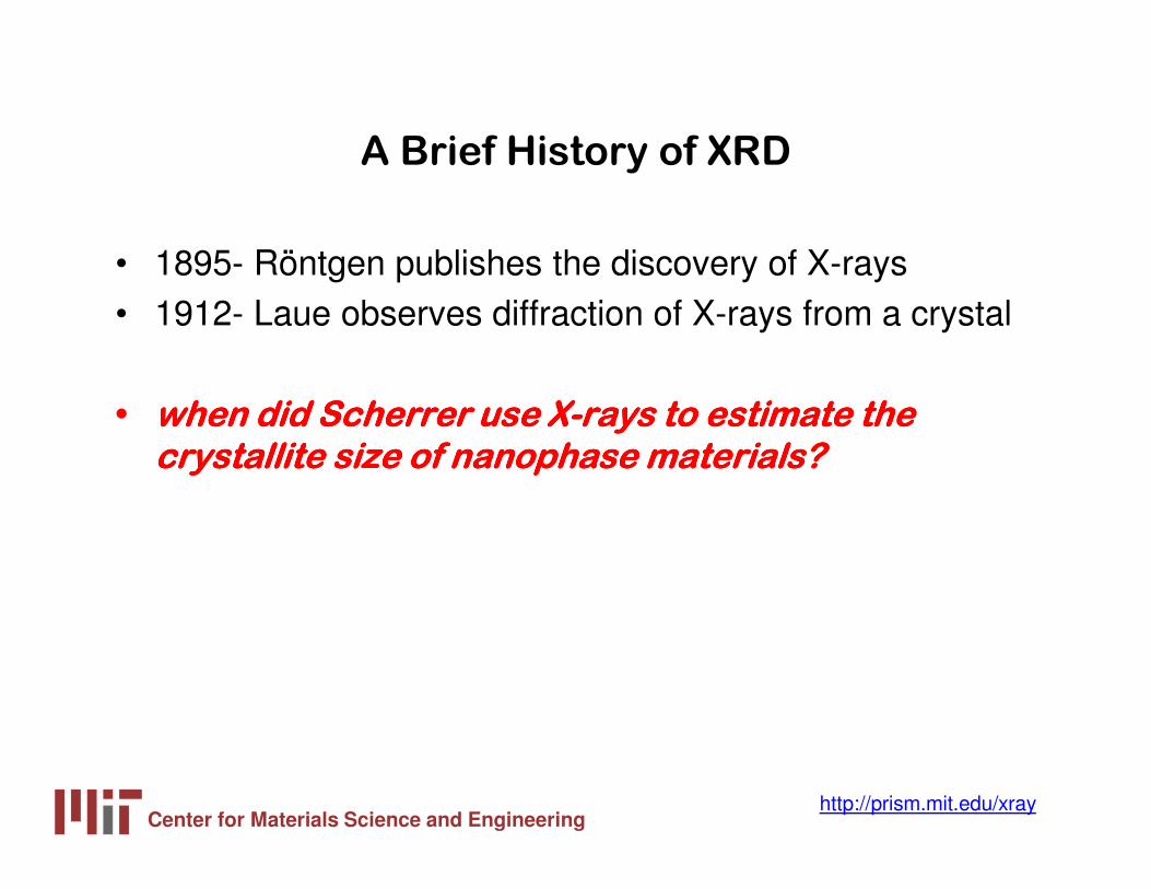
A Brief History of XRD
• 1895- Röntgen publishes the discovery of X-rays• 1912- Laue observes diffraction of X-rays from a crystal
• when did Scherrer use Xwhen did Scherrer use Xwhen did Scherrer use Xwhen did Scherrer use X----rays to estimate the rays to estimate the rays to estimate the rays to estimate the crystallite size of nanophase materials?crystallite size of nanophase materials?crystallite size of nanophase materials?crystallite size of nanophase materials?

Center for Materials Science and Engineeringhttp://prism.mit.edu/xray
The Scherrer Equation was published in 1918
• Peak width (B) is inversely proportional to crystallite size (L)
• P. Scherrer, “Bestimmung der Grösse und der inneren Struktur von Kolloidteilchen mittels Röntgenstrahlen,” Nachr. Ges. Wiss. Göttingen 26(1918) pp 98-100.
• J.I. Langford and A.J.C. Wilson, “Scherrer after Sixty Years: A Survey and Some New Results in the Determination of Crystallite Size,” J. Appl. Cryst.
11 (1978) pp 102-113.
( )θ
λθ
cos2
L
KB =
Center for Materials Science and Engineeringhttp://prism.mit.edu/xray
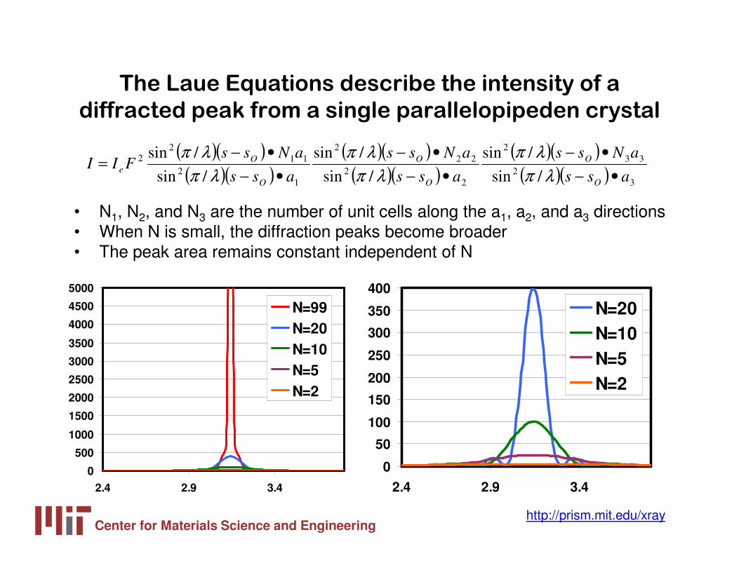
The Laue Equations describe the intensity of a
diffracted peak from a single parallelopipeden crystal
• N1, N2, and N3 are the number of unit cells along the a1, a2, and a3 directions• When N is small, the diffraction peaks become broader• The peak area remains constant independent of N
( )( )( )( )
( )( )( )( )
( )( )( )( ) 3
2
33
2
2
2
22
2
1
2
11
2
2
/sin
/sin
/sin
/sin
/sin
/sin
ass
aNss
ass
aNss
ass
aNssFII
O
O
O
O
O
O
e•−
•−
•−
•−
•−
•−=
λπ
λπ
λπ
λπ
λπ
λπ
0
500
1000
1500
2000
2500
3000
3500
4000
4500
5000
2.4 2.9 3.4
N=99N=20N=10N=5N=2
0
50
100
150
200
250
300
350
400
2.4 2.9 3.4
N=20N=10N=5N=2
Center for Materials Science and Engineeringhttp://prism.mit.edu/xray
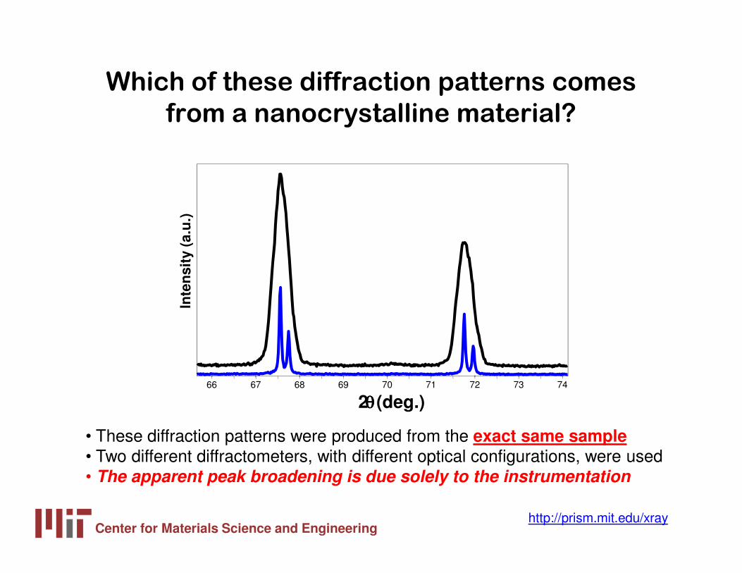
Which of these diffraction patterns comes
from a nanocrystalline material?
66 67 68 69 70 71 72 73 74
2θθθθ (deg.)
Inte
nsi
ty (
a.u
.)
• These diffraction patterns were produced from the exact same sample• Two different diffractometers, with different optical configurations, were used• The apparent peak broadening is due solely to the instrumentation

Center for Materials Science and Engineeringhttp://prism.mit.edu/xray
Many factors may contribute to
the observed peak profile
• Instrumental Peak Profile• Crystallite Size• Microstrain
– Non-uniform Lattice Distortions– Faulting– Dislocations– Antiphase Domain Boundaries– Grain Surface Relaxation
• Solid Solution Inhomogeneity• Temperature Factors
• The peak profile is a convolution of the profiles from all of
these contributions
Center for Materials Science and Engineeringhttp://prism.mit.edu/xray
Instrument and Sample Contributions to the
Peak Profile must be Deconvoluted
• In order to analyze crystallite size, we must deconvolute:– Instrumental Broadening FW(I)
• also referred to as the Instrumental Profile, Instrumental FWHM Curve, Instrumental Peak Profile
– Specimen Broadening FW(S)• also referred to as the Sample Profile, Specimen Profile
• We must then separate the different contributions to specimen broadening– Crystallite size and microstrain broadening of diffraction peaks
Center for Materials Science and Engineeringhttp://prism.mit.edu/xray
Contributions to Peak Profile
1. Peak broadening due to crystallite size2. Peak broadening due to the instrumental profile3. Which instrument to use for nanophase analysis4. Peak broadening due to microstrain
• the different types of microstrain
• Peak broadening due to solid solution inhomogeneity and due to temperature factors
Center for Materials Science and Engineeringhttp://prism.mit.edu/xray
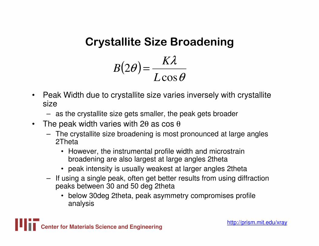
Crystallite Size Broadening
• Peak Width due to crystallite size varies inversely with crystallite size– as the crystallite size gets smaller, the peak gets broader
• The peak width varies with 2θ as cos θ– The crystallite size broadening is most pronounced at large angles
2Theta• However, the instrumental profile width and microstrain
broadening are also largest at large angles 2theta• peak intensity is usually weakest at larger angles 2theta
– If using a single peak, often get better results from using diffraction peaks between 30 and 50 deg 2theta
• below 30deg 2theta, peak asymmetry compromises profile analysis
( )θ
λθ
cos2
L
KB =

Center for Materials Science and Engineeringhttp://prism.mit.edu/xray
The Scherrer Constant, K
• The constant of proportionality, K (the Scherrer constant) depends on the how the width is determined, the shape of the crystal, and the size distribution– the most common values for K are:
• 0.94 for FWHM of spherical crystals with cubic symmetry• 0.89 for integral breadth of spherical crystals w/ cubic symmetry• 1, because 0.94 and 0.89 both round up to 1
– K actually varies from 0.62 to 2.08• For an excellent discussion of K, refer to JI Langford and AJC
Wilson, “Scherrer after sixty years: A survey and some new results in the determination of crystallite size,” J. Appl. Cryst. 11(1978) p102-113.
( )θ
λθ
cos2
L
KB = ( )
θ
λθ
cos
94.02
LB =

Center for Materials Science and Engineeringhttp://prism.mit.edu/xray
Factors that affect K and crystallite size
analysis
• how the peak width is defined • how crystallite size is defined• the shape of the crystal • the size distribution
Center for Materials Science and Engineeringhttp://prism.mit.edu/xray
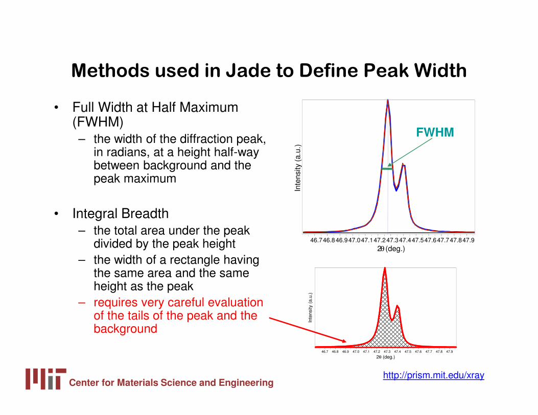
46.7 46.8 46.9 47.0 47.1 47.2 47.3 47.4 47.5 47.6 47.7 47.8 47.9
2θ (deg.)
Inte
nsity
(a.
u.)
Methods used in Jade to Define Peak Width
• Full Width at Half Maximum (FWHM)– the width of the diffraction peak,
in radians, at a height half-way between background and the peak maximum
• Integral Breadth– the total area under the peak
divided by the peak height– the width of a rectangle having
the same area and the same height as the peak
– requires very careful evaluation of the tails of the peak and the background
46.746.846.947.047.147.247.347.447.547.647.747.847.92θ (deg.)
Inte
nsity
(a.
u.)
FWHM
Center for Materials Science and Engineeringhttp://prism.mit.edu/xray
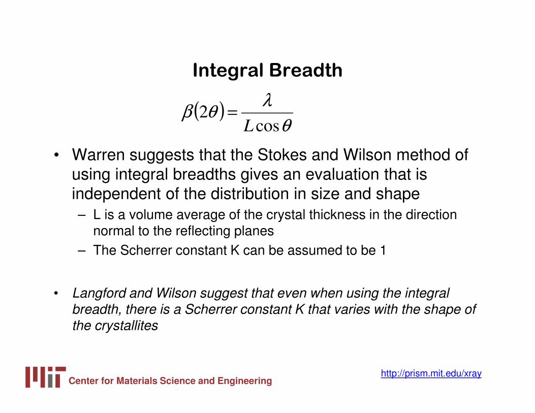
Integral Breadth
• Warren suggests that the Stokes and Wilson method of using integral breadths gives an evaluation that is independent of the distribution in size and shape– L is a volume average of the crystal thickness in the direction
normal to the reflecting planes– The Scherrer constant K can be assumed to be 1
• Langford and Wilson suggest that even when using the integral breadth, there is a Scherrer constant K that varies with the shape of the crystallites
( )θ
λθβ
cos2
L=
Center for Materials Science and Engineeringhttp://prism.mit.edu/xray
Other methods used to determine peak width
• These methods are used in more the variance methods, such as Warren-Averbach analysis– Most often used for dislocation and defect density analysis of metals– Can also be used to determine the crystallite size distribution– Requires no overlap between neighboring diffraction peaks
• Variance-slope– the slope of the variance of the line profile as a function of the range of
integration
• Variance-intercept– negative initial slope of the Fourier transform of the normalized line
profile
Center for Materials Science and Engineeringhttp://prism.mit.edu/xray
How is Crystallite Size Defined
• Usually taken as the cube root of the volume of a crystallite– assumes that all crystallites have the same size and shape
• For a distribution of sizes, the mean size can be defined as– the mean value of the cube roots of the individual crystallite volumes– the cube root of the mean value of the volumes of the individual
crystallites
• Scherrer method (using FWHM) gives the ratio of the root-mean-fourth-power to the root-mean-square value of the thickness
• Stokes and Wilson method (using integral breadth) determines the volume average of the thickness of the crystallites measured perpendicular to the reflecting plane
• The variance methods give the ratio of the total volume of the crystallites to the total area of their projection on a plane parallel to the reflecting planes
Center for Materials Science and Engineeringhttp://prism.mit.edu/xray
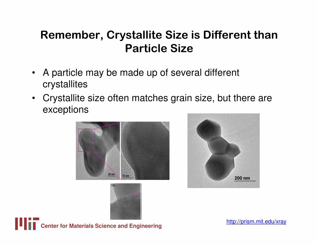
Remember, Crystallite Size is Different than
Particle Size
• A particle may be made up of several different crystallites
• Crystallite size often matches grain size, but there are exceptions
Center for Materials Science and Engineeringhttp://prism.mit.edu/xray
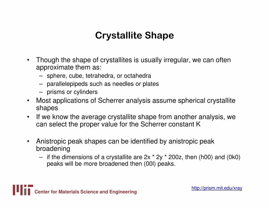
Crystallite Shape
• Though the shape of crystallites is usually irregular, we can often approximate them as:– sphere, cube, tetrahedra, or octahedra– parallelepipeds such as needles or plates– prisms or cylinders
• Most applications of Scherrer analysis assume spherical crystallite shapes
• If we know the average crystallite shape from another analysis, we can select the proper value for the Scherrer constant K
• Anistropic peak shapes can be identified by anistropic peak broadening– if the dimensions of a crystallite are 2x * 2y * 200z, then (h00) and (0k0)
peaks will be more broadened then (00l) peaks.
Center for Materials Science and Engineeringhttp://prism.mit.edu/xray
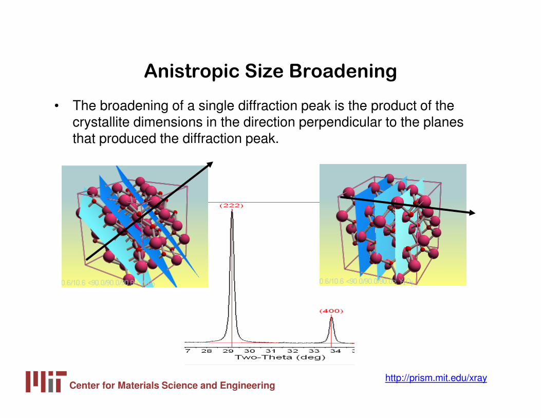
Anistropic Size Broadening
• The broadening of a single diffraction peak is the product of the crystallite dimensions in the direction perpendicular to the planes that produced the diffraction peak.
Center for Materials Science and Engineeringhttp://prism.mit.edu/xray
Crystallite Size Distribution
• is the crystallite size narrowly or broadly distributed?• is the crystallite size unimodal?
• XRD is poorly designed to facilitate the analysis of crystallites with a broad or multimodal size distribution
• Variance methods, such as Warren-Averbach, can be used to quantify a unimodal size distribution– Otherwise, we try to accommodate the size distribution in the Scherrer
constant– Using integral breadth instead of FWHM may reduce the effect of
crystallite size distribution on the Scherrer constant K and therefore the crystallite size analysis
Center for Materials Science and Engineeringhttp://prism.mit.edu/xray
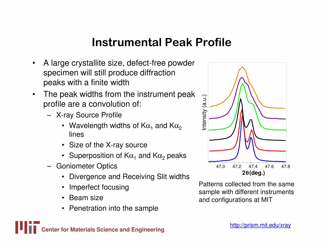
Instrumental Peak Profile
• A large crystallite size, defect-free powder specimen will still produce diffraction peaks with a finite width
• The peak widths from the instrument peak profile are a convolution of:– X-ray Source Profile
• Wavelength widths of Kα1 and Kα2lines
• Size of the X-ray source• Superposition of Kα1 and Kα2 peaks
– Goniometer Optics• Divergence and Receiving Slit widths• Imperfect focusing• Beam size• Penetration into the sample
47.0 47.2 47.4 47.6 47.8
2θθθθ (deg.)
Inte
nsity
(a.
u.)
Patterns collected from the same sample with different instruments and configurations at MIT
Center for Materials Science and Engineeringhttp://prism.mit.edu/xray
What Instrument to Use?
• The instrumental profile determines the upper limit of crystallite size that can be evaluated– if the Instrumental peak width is much larger than the broadening
due to crystallite size, then we cannot accurately determine crystallite size
– For analyzing larger nanocrystallites, it is important to use the instrument with the smallest instrumental peak width
• Very small nanocrystallites produce weak signals– the specimen broadening will be significantly larger than the
instrumental broadening– the signal:noise ratio is more important than the instrumental
profile
Center for Materials Science and Engineeringhttp://prism.mit.edu/xray
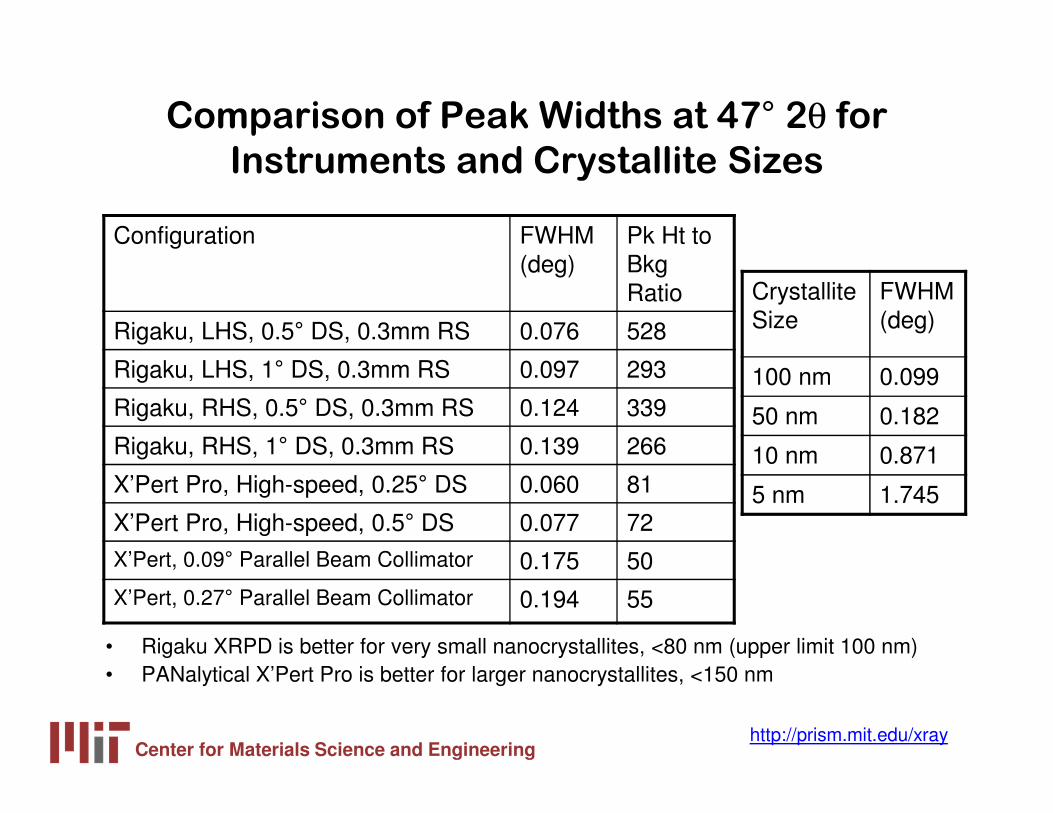
Comparison of Peak Widths at 47° 2θ for
Instruments and Crystallite Sizes
• Rigaku XRPD is better for very small nanocrystallites, <80 nm (upper limit 100 nm)• PANalytical X’Pert Pro is better for larger nanocrystallites, <150 nm
Configuration FWHM (deg)
Pk Ht to Bkg Ratio
Rigaku, LHS, 0.5° DS, 0.3mm RS 0.076 528
Rigaku, LHS, 1° DS, 0.3mm RS 0.097 293
Rigaku, RHS, 0.5° DS, 0.3mm RS 0.124 339
Rigaku, RHS, 1° DS, 0.3mm RS 0.139 266
X’Pert Pro, High-speed, 0.25° DS 0.060 81
X’Pert Pro, High-speed, 0.5° DS 0.077 72
X’Pert, 0.09° Parallel Beam Collimator 0.175 50
X’Pert, 0.27° Parallel Beam Collimator 0.194 55
Crystallite Size
FWHM (deg)
100 nm 0.099
50 nm 0.182
10 nm 0.871
5 nm 1.745

Center for Materials Science and Engineeringhttp://prism.mit.edu/xray
Other Instrumental Considerations
for Thin Films
• The irradiated area greatly affects the intensity of high angle diffraction peaks– GIXD or variable divergence slits on the
PANalytical X’Pert Pro will maintain a constant irradiated area, increasing the signal for high angle diffraction peaks
– both methods increase the instrumental FWHM
• Bragg-Brentano geometry only probes crystallite dimensions through the thickness of the film– in order to probe lateral (in-plane) crystallite sizes,
need to collect diffraction patterns at different tilts– this requires the use of parallel-beam optics on the
PANalytical X’Pert Pro, which have very large FWHM and poor signal:noise ratios
Center for Materials Science and Engineeringhttp://prism.mit.edu/xray
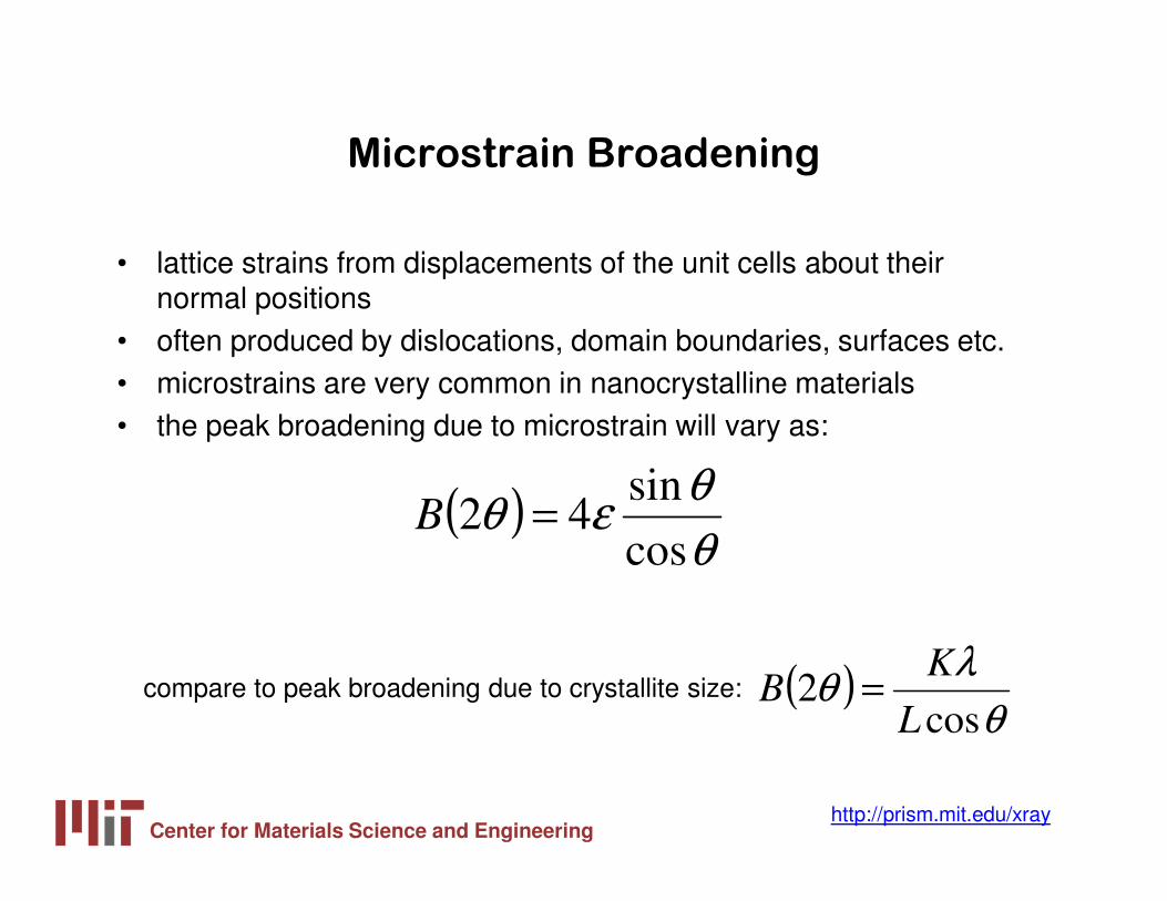
Microstrain Broadening
• lattice strains from displacements of the unit cells about their normal positions
• often produced by dislocations, domain boundaries, surfaces etc.• microstrains are very common in nanocrystalline materials• the peak broadening due to microstrain will vary as:
( )θ
θεθ
cos
sin42 =B
compare to peak broadening due to crystallite size: ( )θ
λθ
cos2
L
KB =
Center for Materials Science and Engineeringhttp://prism.mit.edu/xray
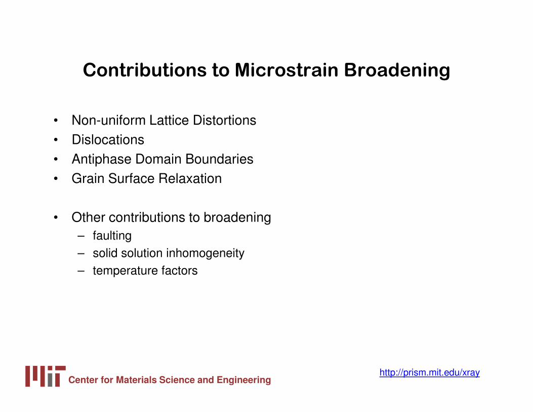
Contributions to Microstrain Broadening
• Non-uniform Lattice Distortions• Dislocations• Antiphase Domain Boundaries• Grain Surface Relaxation
• Other contributions to broadening– faulting– solid solution inhomogeneity– temperature factors
Center for Materials Science and Engineeringhttp://prism.mit.edu/xray
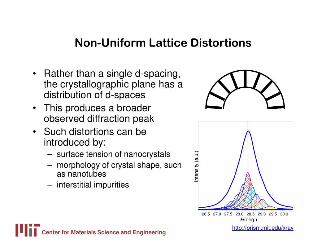
Non-Uniform Lattice Distortions
• Rather than a single d-spacing, the crystallographic plane has a distribution of d-spaces
• This produces a broader observed diffraction peak
• Such distortions can be introduced by: – surface tension of nanocrystals– morphology of crystal shape, such
as nanotubes– interstitial impurities
26.5 27.0 27.5 28.0 28.5 29.0 29.5 30.02θ(deg.)
Inte
nsity
(a.
u.)

Center for Materials Science and Engineeringhttp://prism.mit.edu/xray
Antiphase Domain Boundaries
• Formed during the ordering of a material that goes through an order-disorder transformation
• The fundamental peaks are not affected• the superstructure peaks are broadened
– the broadening of superstructure peaks varies with hkl
Center for Materials Science and Engineeringhttp://prism.mit.edu/xray
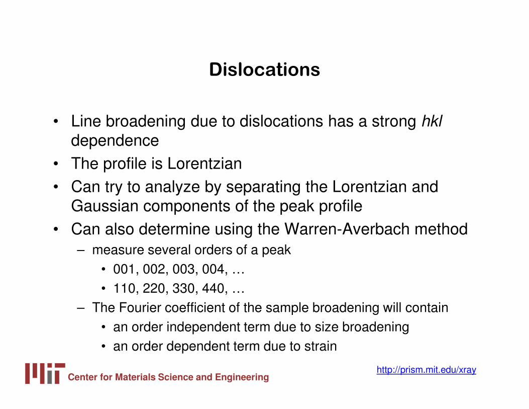
Dislocations
• Line broadening due to dislocations has a strong hkl
dependence• The profile is Lorentzian• Can try to analyze by separating the Lorentzian and
Gaussian components of the peak profile• Can also determine using the Warren-Averbach method
– measure several orders of a peak• 001, 002, 003, 004, …• 110, 220, 330, 440, …
– The Fourier coefficient of the sample broadening will contain • an order independent term due to size broadening • an order dependent term due to strain
Center for Materials Science and Engineeringhttp://prism.mit.edu/xray
Faulting
• Broadening due to deformation faulting and twin faulting will convolute with the particle size Fourier coefficient– The particle size coefficient determined by Warren-Averbach
analysis actually contains contributions from the crystallite size and faulting
– the fault contribution is hkl dependent, while the size contribution should be hkl independent (assuming isotropic crystallite shape)
– the faulting contribution varies as a function of hkl dependent on the crystal structure of the material (fcc vs bcc vs hcp)
– See Warren, 1969, for methods to separate the contributions from deformation and twin faulting

Center for Materials Science and Engineeringhttp://prism.mit.edu/xray
CeO219 nm
45 46 47 48 49 50 51 52
2θθθθ (deg.)
Inte
nsity
(a.
u.)
ZrO246nm
CexZr1-xO20<x<1
Solid Solution Inhomogeneity
• Variation in the composition of a solid solution can create a distribution of d-spacing for a crystallographic plane– Similar to the d-spacing distribution created from microstrain due
to non-uniform lattice distortions
Center for Materials Science and Engineeringhttp://prism.mit.edu/xray
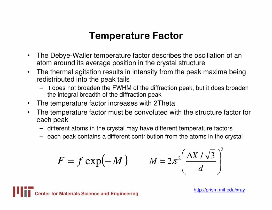
Temperature Factor
• The Debye-Waller temperature factor describes the oscillation of an atom around its average position in the crystal structure
• The thermal agitation results in intensity from the peak maxima being redistributed into the peak tails– it does not broaden the FWHM of the diffraction peak, but it does broaden
the integral breadth of the diffraction peak• The temperature factor increases with 2Theta• The temperature factor must be convoluted with the structure factor for
each peak– different atoms in the crystal may have different temperature factors– each peak contains a different contribution from the atoms in the crystal
( )MfF −= exp
2
2 3/2
∆=
d
XM π
Center for Materials Science and Engineeringhttp://prism.mit.edu/xray
Determining the Sample Broadening due to
crystallite size
• The sample profile FW(S) can be deconvoluted from the instrumental profile FW(I) either numerically or by Fourier transform
• In Jade size and strain analysis– you individually profile fit every diffraction peak– deconvolute FW(I) from the peak profile functions to isolate FW(S) – execute analyses on the peak profile functions rather than on the raw
data• Jade can also use iterative folding to deconvolute FW(I) from the
entire observed diffraction pattern– this produces an entire diffraction pattern without an instrumental
contribution to peak widths– this does not require fitting of individual diffraction peaks – folding increases the noise in the observed diffraction pattern
• Warren Averbach analyses operate on the Fourier transform of the diffraction peak– take Fourier transform of peak profile functions or of raw data
Center for Materials Science and Engineeringhttp://prism.mit.edu/xray
Analysis using MDI Jade
• The data analysis package Jade is designed to use empirical peak profile fitting to estimate crystallite size and/or microstrain
• Three Primary Components– Profile Fitting Techniques– Instrumental FWHM Curve– Size & Strain Analysis
• Scherrer method• Williamson-Hall method
Center for Materials Science and Engineeringhttp://prism.mit.edu/xray
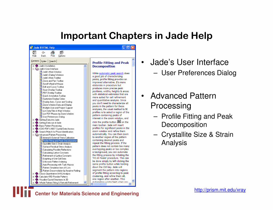
Important Chapters in Jade Help
• Jade’s User Interface– User Preferences Dialog
• Advanced Pattern Processing– Profile Fitting and Peak
Decomposition– Crystallite Size & Strain
Analysis
Center for Materials Science and Engineeringhttp://prism.mit.edu/xray
28.5 29.0 29.5 30.0
2θ (deg.)In
tens
ity (
a.u.
)
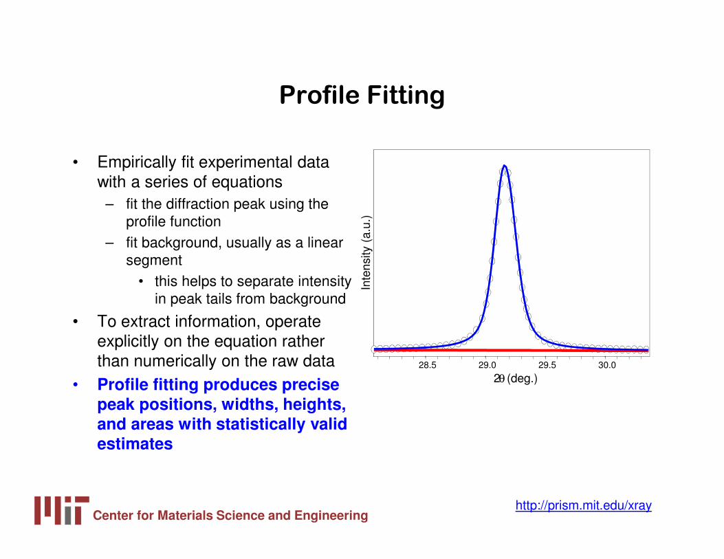
Profile Fitting
• Empirically fit experimental data with a series of equations
– fit the diffraction peak using the profile function
– fit background, usually as a linear segment
• this helps to separate intensity in peak tails from background
• To extract information, operate explicitly on the equation rather than numerically on the raw data
• Profile fitting produces precise peak positions, widths, heights, and areas with statistically valid estimates

Center for Materials Science and Engineeringhttp://prism.mit.edu/xray
Profile Functions
• Diffraction peaks are usually the convolution of Gaussian and Lorentzian components
• Some techniques try to deconvolute the Gaussian and Lorentzian contributions to each diffraction peak; this is very difficult
• More typically, data are fit with a profile function that is a pseudo-Voigt or Pearson VII curve
– pseudo-Voigt is a linear combination of Gaussian and Lorentzian components• a true Voigt curve is a convolution of the Gaussian and Lorentzian
components; this is more difficult to implement computationally– Pearson VII is an exponential mixing of Gaussian and Lorentzian components
• SA Howard and KD Preston, “Profile Fitting of Powder Diffraction Patterns,”, Reviews in Mineralogy vol 20: Modern Powder Diffraction, Mineralogical Society of America, Washington DC, 1989.
Center for Materials Science and Engineeringhttp://prism.mit.edu/xray
Important Tips for Profile Fitting
• Do not process the data before profile fitting– do not smooth the data– do not fit and remove the background– do not strip Ka2 peaks
• Load the appropriate PDF reference patterns for your phases of interest
• Zoom in so that as few peaks as possible, plus some background, is visible– Fit as few peaks simultaneously as possible– preferably fit only 1 peak at a time
• Constrain variables when necessary to enhance the stability of the refinement
Center for Materials Science and Engineeringhttp://prism.mit.edu/xray
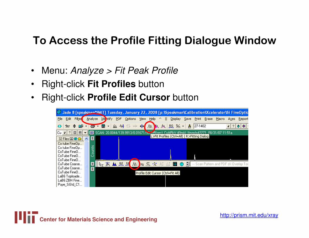
To Access the Profile Fitting Dialogue Window
• Menu: Analyze > Fit Peak Profile
• Right-click Fit Profiles button• Right-click Profile Edit Cursor button
Center for Materials Science and Engineeringhttp://prism.mit.edu/xray
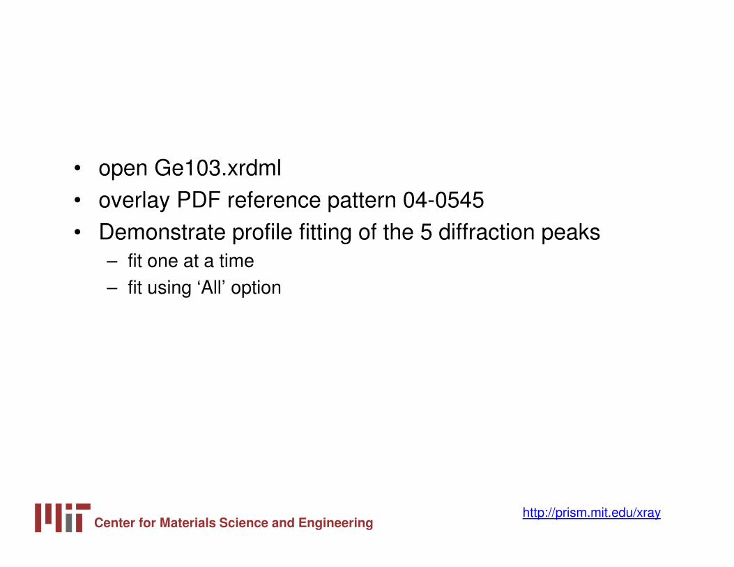
• open Ge103.xrdml• overlay PDF reference pattern 04-0545• Demonstrate profile fitting of the 5 diffraction peaks
– fit one at a time– fit using ‘All’ option
Center for Materials Science and Engineeringhttp://prism.mit.edu/xray
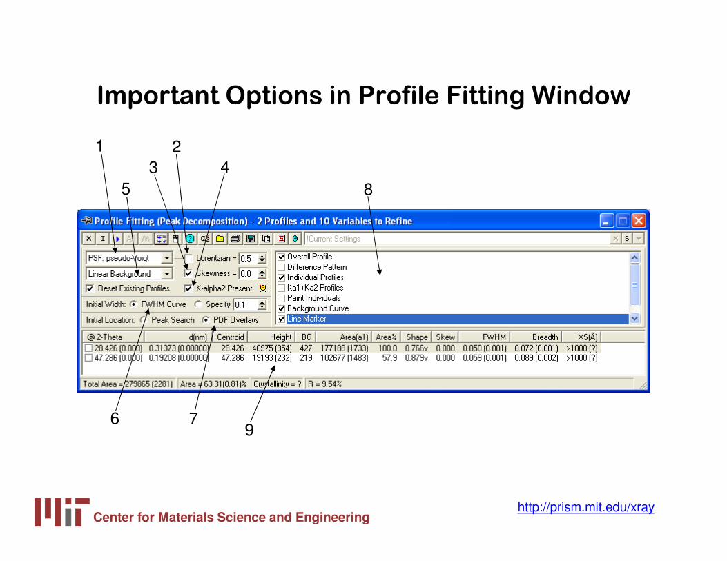
Important Options in Profile Fitting Window
1
53
24
8
6 79

Center for Materials Science and Engineeringhttp://prism.mit.edu/xray
1. Profile Shape Function
• select the equation that will be used to fit diffraction peaks• Gaussian:
– more appropriate for fitting peaks with a rounder top– strain distribution tends to broaden the peak as a Gaussian
• Lorentzian:– more appropriate for fitting peaks with a sharper top– size distribution tends to broaden the peak as a Lorentzian– dislocations also create a Lorentzian component to the peak broadening
• The instrumental profile and peak shape are often a combination of Gaussian and Lorentzian contributions
• pseudo-Voigt:– emphasizes Guassian contribution– preferred when strain broadening dominates
• Pearson VII:– emphasize Lorentzian contribution– preferred when size broadening dominates
Center for Materials Science and Engineeringhttp://prism.mit.edu/xray
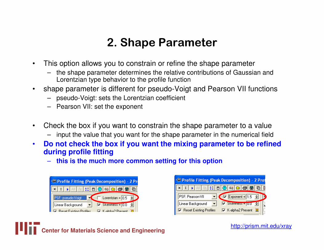
2. Shape Parameter
• This option allows you to constrain or refine the shape parameter– the shape parameter determines the relative contributions of Gaussian and
Lorentzian type behavior to the profile function• shape parameter is different for pseudo-Voigt and Pearson VII functions
– pseudo-Voigt: sets the Lorentzian coefficient– Pearson VII: set the exponent
• Check the box if you want to constrain the shape parameter to a value– input the value that you want for the shape parameter in the numerical field
• Do not check the box if you want the mixing parameter to be refined during profile fitting
– this is the much more common setting for this option
Center for Materials Science and Engineeringhttp://prism.mit.edu/xray
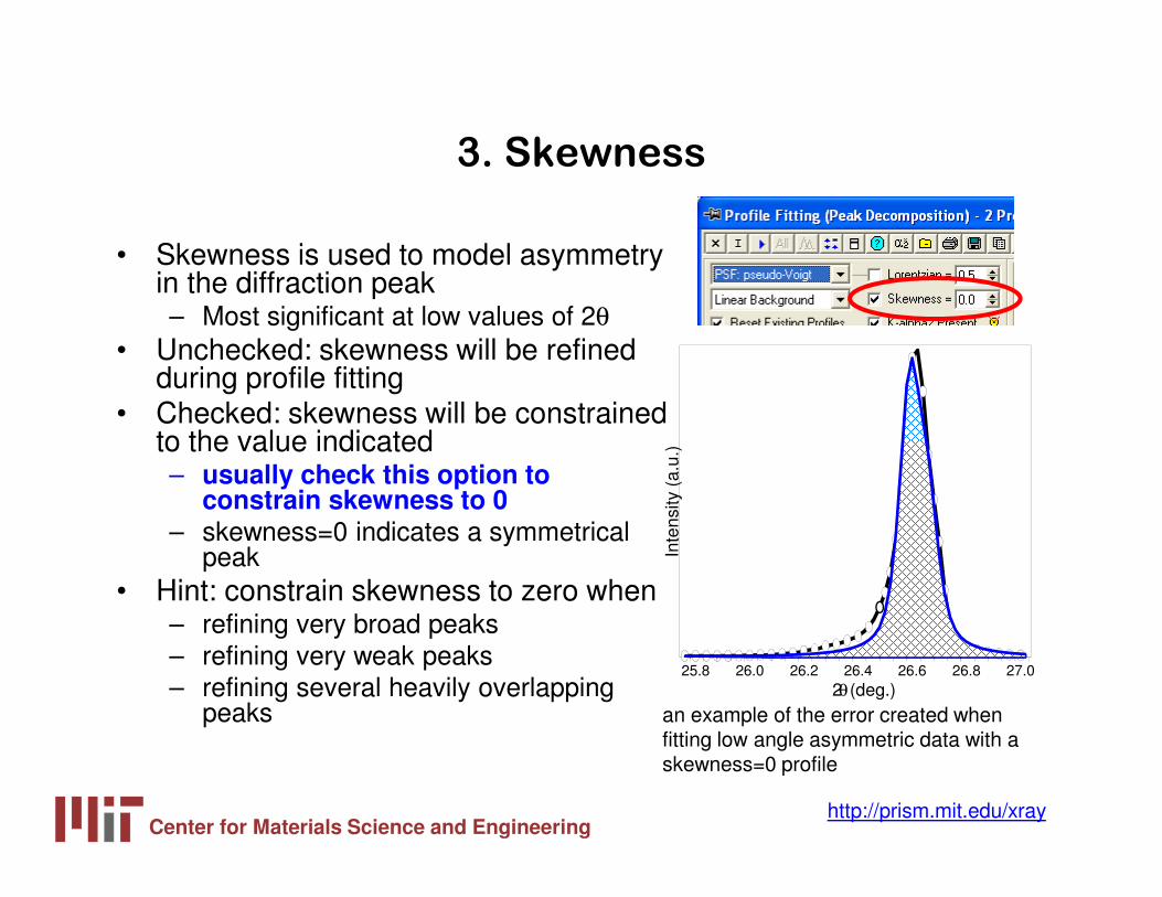
3. Skewness
• Skewness is used to model asymmetry in the diffraction peak– Most significant at low values of 2θ
• Unchecked: skewness will be refined during profile fitting
• Checked: skewness will be constrained to the value indicated– usually check this option to
constrain skewness to 0– skewness=0 indicates a symmetrical
peak• Hint: constrain skewness to zero when
– refining very broad peaks– refining very weak peaks– refining several heavily overlapping
peaks an example of the error created when fitting low angle asymmetric data with a skewness=0 profile
25.8 26.0 26.2 26.4 26.6 26.8 27.02θ (deg.)
Inte
nsity
(a.
u.)
Center for Materials Science and Engineeringhttp://prism.mit.edu/xray
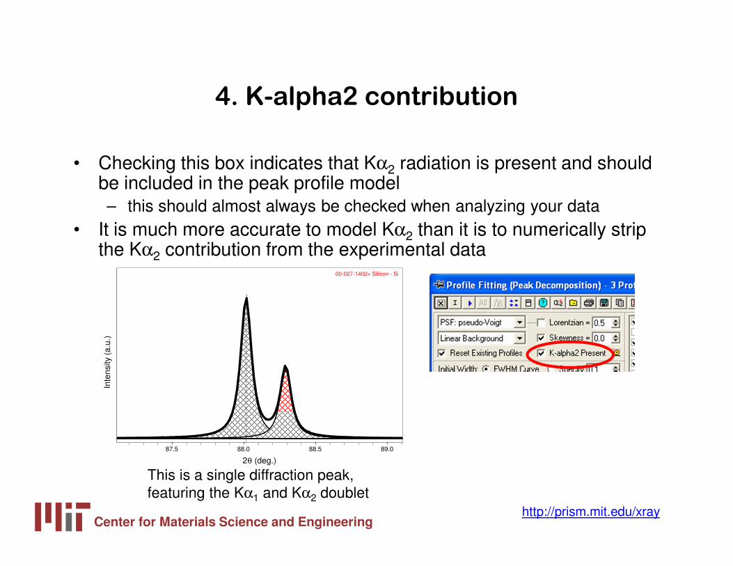
87.5 88.0 88.5 89.0
2θ (deg.)
Inte
nsity
(a.
u.)
00-027-1402> Silicon - Si
4. K-alpha2 contribution
• Checking this box indicates that Kα2 radiation is present and should be included in the peak profile model– this should almost always be checked when analyzing your data
• It is much more accurate to model Kα2 than it is to numerically strip the Kα2 contribution from the experimental data
This is a single diffraction peak, featuring the Kα1 and Kα2 doublet
Center for Materials Science and Engineeringhttp://prism.mit.edu/xray
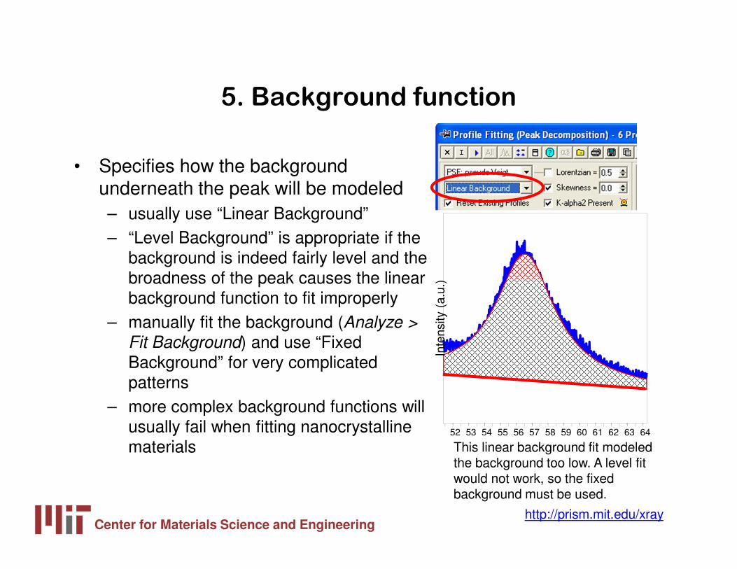
52 53 54 55 56 57 58 59 60 61 62 63 64
2θ(deg.)In
tens
ity (
a.u.
)
5. Background function
• Specifies how the background underneath the peak will be modeled– usually use “Linear Background”– “Level Background” is appropriate if the
background is indeed fairly level and the broadness of the peak causes the linear background function to fit improperly
– manually fit the background (Analyze >
Fit Background) and use “Fixed Background” for very complicated patterns
– more complex background functions will usually fail when fitting nanocrystalline materials This linear background fit modeled
the background too low. A level fit would not work, so the fixed background must be used.
Center for Materials Science and Engineeringhttp://prism.mit.edu/xray
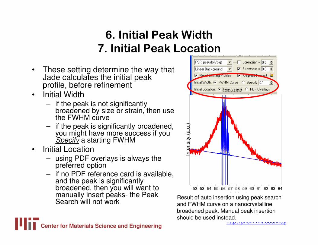
52 53 54 55 56 57 58 59 60 61 62 63 64
2θ(deg.)In
tens
ity (
a.u.
)
6. Initial Peak Width
7. Initial Peak Location
• These setting determine the way that Jade calculates the initial peak profile, before refinement
• Initial Width– if the peak is not significantly
broadened by size or strain, then use the FWHM curve
– if the peak is significantly broadened, you might have more success if you Specify a starting FWHM
• Initial Location– using PDF overlays is always the
preferred option– if no PDF reference card is available,
and the peak is significantly broadened, then you will want to manually insert peaks- the Peak Search will not work
Result of auto insertion using peak search and FWHM curve on a nanocrystalline broadened peak. Manual peak insertion should be used instead.
Center for Materials Science and Engineeringhttp://prism.mit.edu/xray
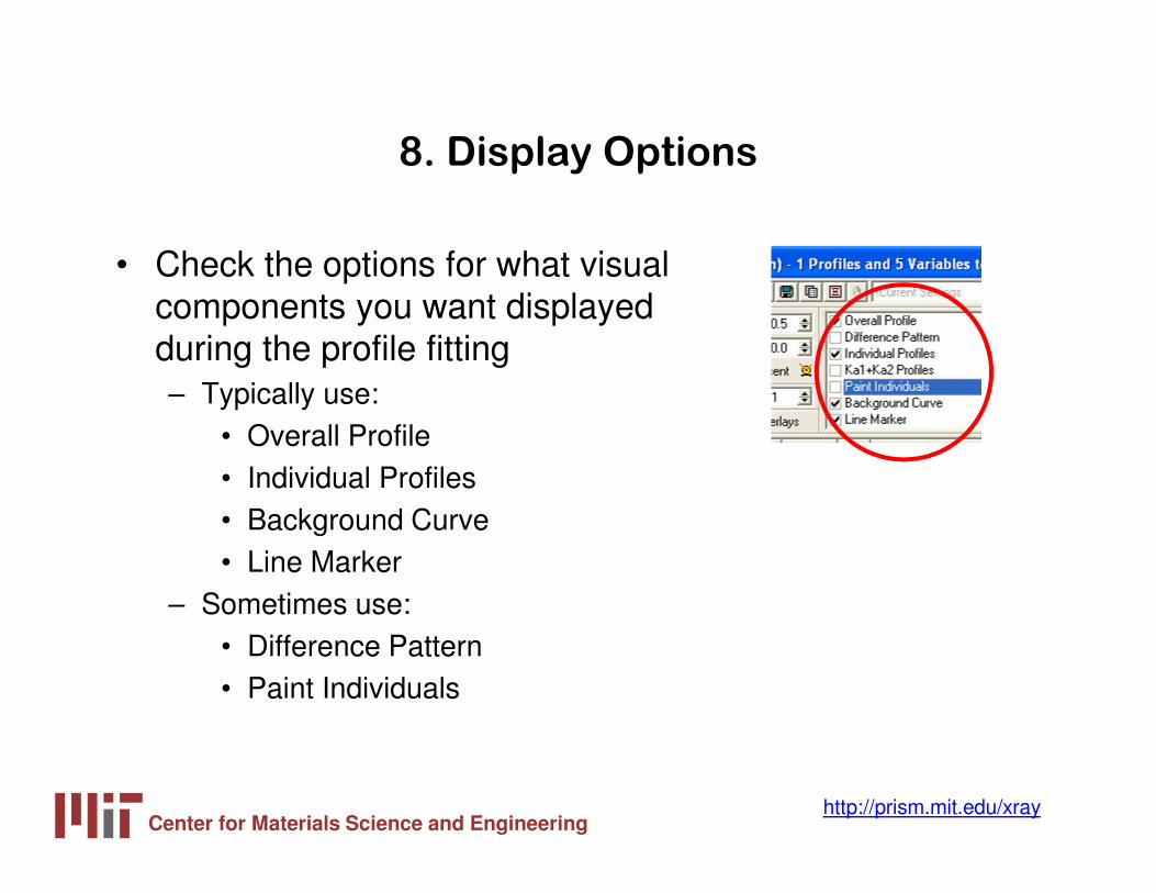
8. Display Options
• Check the options for what visual components you want displayed during the profile fitting– Typically use:
• Overall Profile• Individual Profiles• Background Curve• Line Marker
– Sometimes use:• Difference Pattern• Paint Individuals
Center for Materials Science and Engineeringhttp://prism.mit.edu/xray
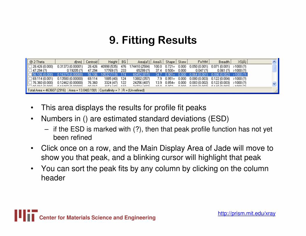
9. Fitting Results
• This area displays the results for profile fit peaks• Numbers in () are estimated standard deviations (ESD)
– if the ESD is marked with (?), then that peak profile function has not yet been refined
• Click once on a row, and the Main Display Area of Jade will move to show you that peak, and a blinking cursor will highlight that peak
• You can sort the peak fits by any column by clicking on the column header
Center for Materials Science and Engineeringhttp://prism.mit.edu/xray
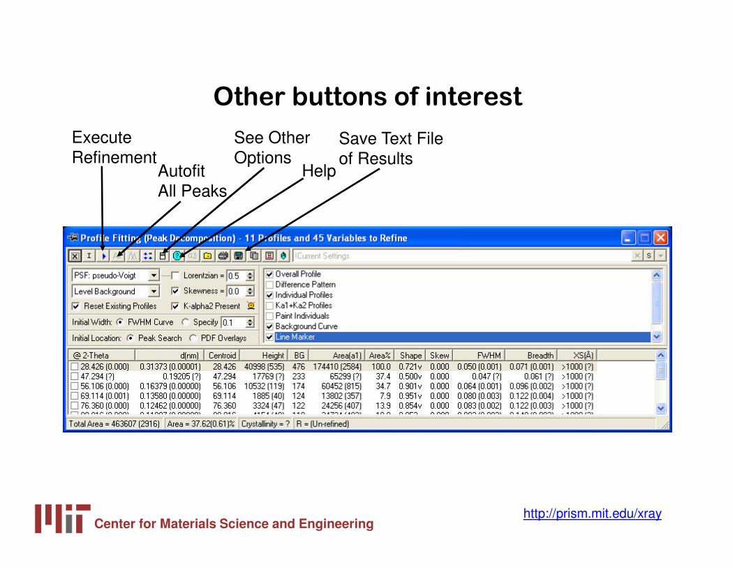
Other buttons of interest
ExecuteRefinement
AutofitAll Peaks
See OtherOptions
Help
Save Text Fileof Results
Center for Materials Science and Engineeringhttp://prism.mit.edu/xray
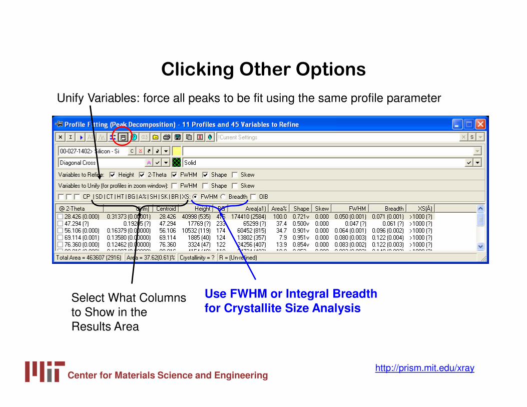
Clicking Other Options
Unify Variables: force all peaks to be fit using the same profile parameter
Use FWHM or Integral Breadth for Crystallite Size Analysis
Select What Columns to Show in the Results Area
Center for Materials Science and Engineeringhttp://prism.mit.edu/xray
Procedure for Profile Fitting a Diffraction
Pattern
1. Open the diffraction pattern2. Overlay the PDF reference3. Zoom in on first peak(s) to analyze4. Open the profile fitting dialogue to configure options5. Refine the profile fit for the first peak(s) 6. Review the quality of profile fit7. Move to next peak(s) and profile fit8. Continue until entire pattern is fit
Center for Materials Science and Engineeringhttp://prism.mit.edu/xray
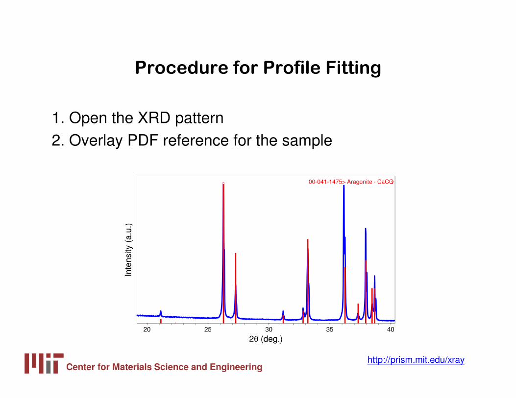
Procedure for Profile Fitting
1. Open the XRD pattern2. Overlay PDF reference for the sample
20 25 30 35 40
2θ (deg.)
Inte
nsity
(a.
u.)
00-041-1475> Aragonite - CaCO3

Center for Materials Science and Engineeringhttp://prism.mit.edu/xray
Procedure for Profile Fitting
3. Zoom in on First Peak to Analyze– try to zoom in on only one peak– be sure to include some background on either side of the peak
25.6 25.7 25.8 25.9 26.0 26.1 26.2 26.3 26.4 26.5 26.6 26.7
2θ (deg.)
Inte
nsity
(a.
u.)
00-041-1475> Aragonite - CaCO3
Center for Materials Science and Engineeringhttp://prism.mit.edu/xray
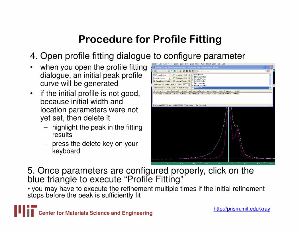
Procedure for Profile Fitting
• when you open the profile fitting dialogue, an initial peak profile curve will be generated
• if the initial profile is not good, because initial width and location parameters were not yet set, then delete it– highlight the peak in the fitting
results– press the delete key on your
keyboard
4. Open profile fitting dialogue to configure parameter
5. Once parameters are configured properly, click on the blue triangle to execute “Profile Fitting”• you may have to execute the refinement multiple times if the initial refinement stops before the peak is sufficiently fit
Center for Materials Science and Engineeringhttp://prism.mit.edu/xray
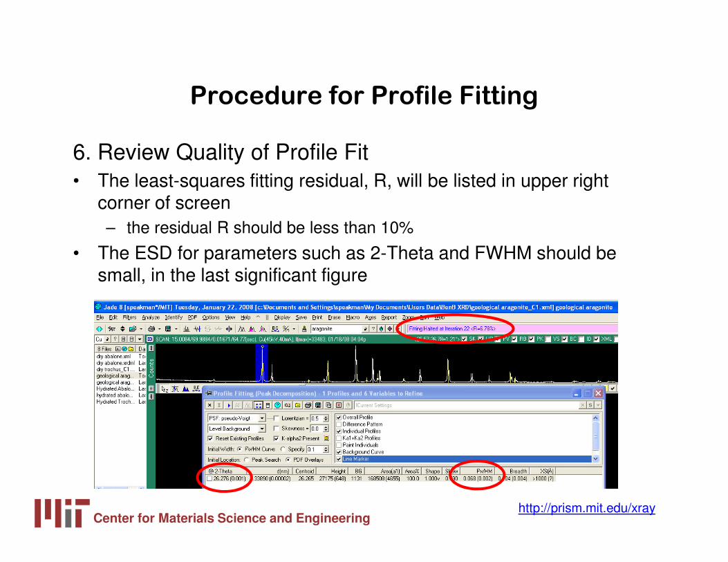
Procedure for Profile Fitting
6. Review Quality of Profile Fit• The least-squares fitting residual, R, will be listed in upper right
corner of screen– the residual R should be less than 10%
• The ESD for parameters such as 2-Theta and FWHM should be small, in the last significant figure
Center for Materials Science and Engineeringhttp://prism.mit.edu/xray
37.0 37.5 38.0 38.5 39.0
2θ (deg.)
Inte
nsity
(a.
u.)
00-041-1475> Aragonite - CaCO 3
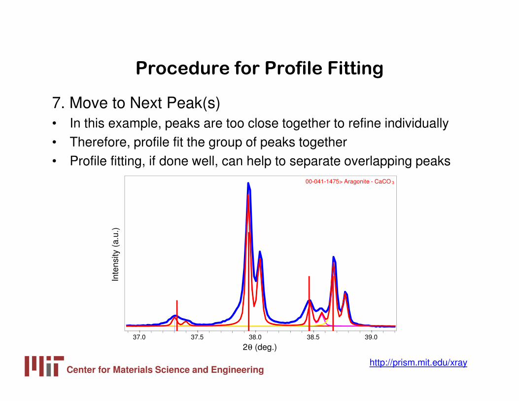
Procedure for Profile Fitting
7. Move to Next Peak(s) • In this example, peaks are too close together to refine individually• Therefore, profile fit the group of peaks together• Profile fitting, if done well, can help to separate overlapping peaks
Center for Materials Science and Engineeringhttp://prism.mit.edu/xray
30 40 50 60
2θ (deg.)
Inte
nsity
(a.
u.)
00-041-1475> Aragonite - CaCO 3
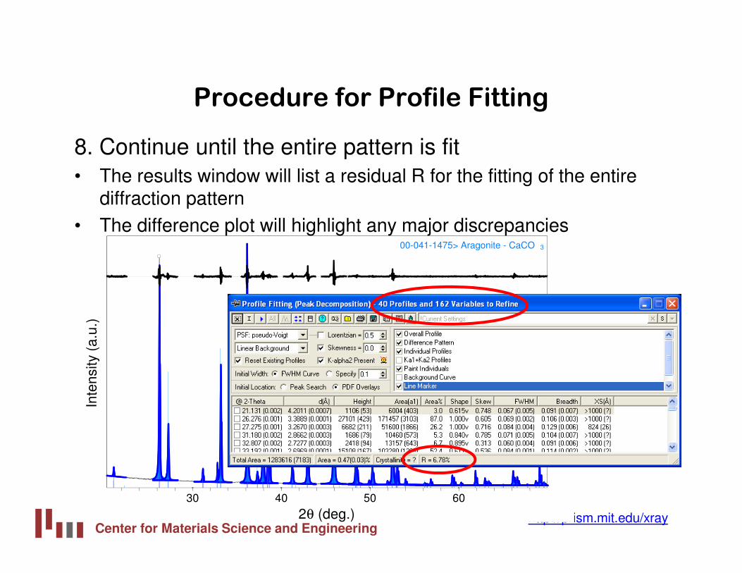
Procedure for Profile Fitting
8. Continue until the entire pattern is fit• The results window will list a residual R for the fitting of the entire
diffraction pattern• The difference plot will highlight any major discrepancies
Center for Materials Science and Engineeringhttp://prism.mit.edu/xray
Instrumental FWHM Calibration Curve
• The instrument itself contributes to the peak profile• Before profile fitting the nanocrystalline phase(s) of
interest – profile fit a calibration standard to determine the
instrumental profile
• Important factors for producing a calibration curve– Use the exact same instrumental conditions
• same optical configuration of diffractometer• same sample preparation geometry• calibration curve should cover the 2theta range of interest for
the specimen diffraction pattern– do not extrapolate the calibration curve
Center for Materials Science and Engineeringhttp://prism.mit.edu/xray
Instrumental FWHM Calibration Curve
• Standard should share characteristics with the nanocrystalline specimen– similar mass absorption coefficient– similar atomic weight– similar packing density
• The standard should not contribute to the diffraction peak profile– macrocrystalline: crystallite size larger than 500 nm– particle size less than 10 microns– defect and strain free
• There are several calibration techniques– Internal Standard– External Standard of same composition– External Standard of different composition

Center for Materials Science and Engineeringhttp://prism.mit.edu/xray
Internal Standard Method for Calibration
• Mix a standard in with your nanocrystalline specimen• a NIST certified standard is preferred
– use a standard with similar mass absorption coefficient– NIST 640c Si– NIST 660a LaB6
– NIST 674b CeO2
– NIST 675 Mica
• standard should have few, and preferably no, overlapping peaks with the specimen– overlapping peaks will greatly compromise accuracy of analysis
Center for Materials Science and Engineeringhttp://prism.mit.edu/xray
Internal Standard Method for Calibration
• Advantages:– know that standard and specimen patterns were collected under
identical circumstances for both instrumental conditions and sample preparation conditions
– the linear absorption coefficient of the mixture is the same for standard and specimen
• Disadvantages: – difficult to avoid overlapping peaks between standard and
broadened peaks from very nanocrystalline materials– the specimen is contaminated– only works with a powder specimen

Center for Materials Science and Engineeringhttp://prism.mit.edu/xray
External Standard Method for Calibration
• If internal calibration is not an option, then use external calibration
• Run calibration standard separately from specimen, keeping as many parameters identical as is possible
• The best external standard is a macrocrystalline specimen of the same phase as your nanocrystalline specimen– How can you be sure that macrocrystalline specimen does not
contribute to peak broadening?
Center for Materials Science and Engineeringhttp://prism.mit.edu/xray
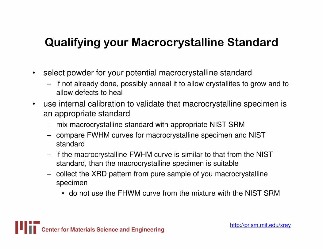
Qualifying your Macrocrystalline Standard
• select powder for your potential macrocrystalline standard– if not already done, possibly anneal it to allow crystallites to grow and to
allow defects to heal
• use internal calibration to validate that macrocrystalline specimen is an appropriate standard– mix macrocrystalline standard with appropriate NIST SRM– compare FWHM curves for macrocrystalline specimen and NIST
standard– if the macrocrystalline FWHM curve is similar to that from the NIST
standard, than the macrocrystalline specimen is suitable– collect the XRD pattern from pure sample of you macrocrystalline
specimen• do not use the FHWM curve from the mixture with the NIST SRM

Center for Materials Science and Engineeringhttp://prism.mit.edu/xray
Disadvantages/Advantages of External Calibration
with a Standard of the Same Composition
• Advantages:– will produce better calibration curve because mass absorption
coefficient, density, molecular weight are the same as your specimen of interest
– can duplicate a mixture in your nanocrystalline specimen– might be able to make a macrocrystalline standard for thin film samples
• Disadvantages: – time consuming– desire a different calibration standard for every different nanocrystalline
phase and mixture– macrocrystalline standard may be hard/impossible to produce– calibration curve will not compensate for discrepancies in instrumental
conditions or sample preparation conditions between the standard and the specimen

Center for Materials Science and Engineeringhttp://prism.mit.edu/xray
External Standard Method of Calibration using
a NIST standard
• As a last resort, use an external standard of a composition that is different than your nanocrystalline specimen– This is actually the most common method used– Also the least accurate method
• Use a certified NIST standard to produce instrumental FWHM calibration curve
Center for Materials Science and Engineeringhttp://prism.mit.edu/xray
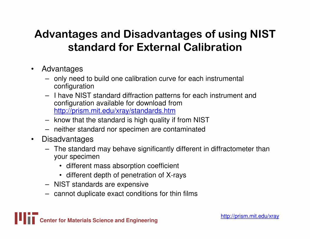
Advantages and Disadvantages of using NIST
standard for External Calibration
• Advantages– only need to build one calibration curve for each instrumental
configuration– I have NIST standard diffraction patterns for each instrument and
configuration available for download from http://prism.mit.edu/xray/standards.htm
– know that the standard is high quality if from NIST– neither standard nor specimen are contaminated
• Disadvantages– The standard may behave significantly different in diffractometer than
your specimen• different mass absorption coefficient• different depth of penetration of X-rays
– NIST standards are expensive– cannot duplicate exact conditions for thin films
Center for Materials Science and Engineeringhttp://prism.mit.edu/xray
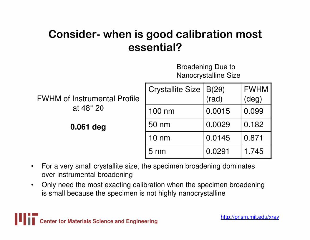
Consider- when is good calibration most
essential?
• For a very small crystallite size, the specimen broadening dominates over instrumental broadening
• Only need the most exacting calibration when the specimen broadening is small because the specimen is not highly nanocrystalline
FWHM of Instrumental Profileat 48° 2θ
0.061 deg
Broadening Due to Nanocrystalline Size
Crystallite Size B(2θ) (rad)
FWHM (deg)
100 nm 0.0015 0.099
50 nm 0.0029 0.182
10 nm 0.0145 0.871
5 nm 0.0291 1.745
Center for Materials Science and Engineeringhttp://prism.mit.edu/xray
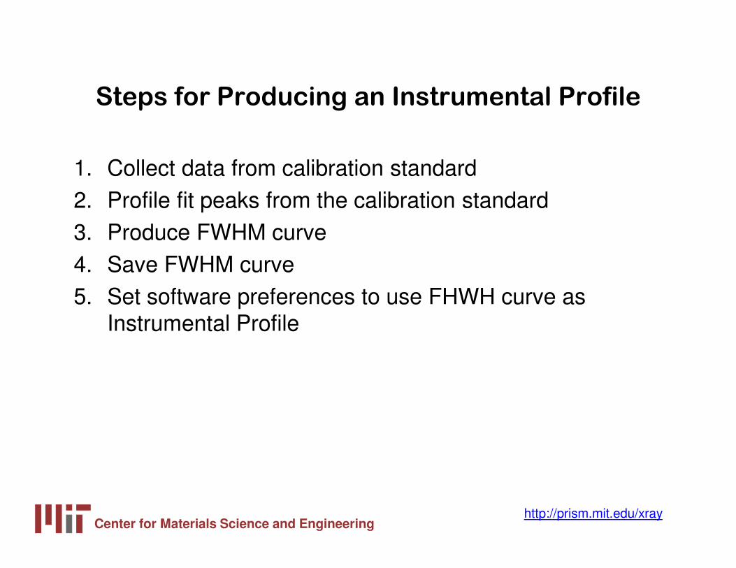
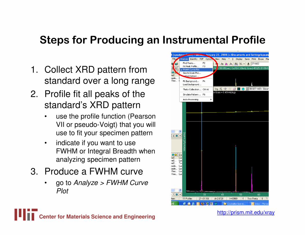
Steps for Producing an Instrumental Profile
1. Collect data from calibration standard2. Profile fit peaks from the calibration standard3. Produce FWHM curve4. Save FWHM curve5. Set software preferences to use FHWH curve as
Instrumental Profile
Center for Materials Science and Engineeringhttp://prism.mit.edu/xray
Steps for Producing an Instrumental Profile
1. Collect XRD pattern from standard over a long range
2. Profile fit all peaks of the standard’s XRD pattern• use the profile function (Pearson
VII or pseudo-Voigt) that you will use to fit your specimen pattern
• indicate if you want to use FWHM or Integral Breadth when analyzing specimen pattern
3. Produce a FWHM curve• go to Analyze > FWHM Curve
Plot
Center for Materials Science and Engineeringhttp://prism.mit.edu/xray
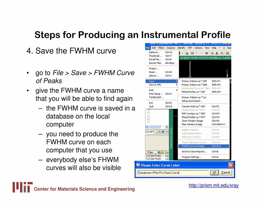
Steps for Producing an Instrumental Profile
4. Save the FWHM curve
• go to File > Save > FWHM Curve of Peaks
• give the FWHM curve a name that you will be able to find again– the FWHM curve is saved in a
database on the local computer
– you need to produce the FWHM curve on each computer that you use
– everybody else’s FHWM curves will also be visible

Center for Materials Science and Engineeringhttp://prism.mit.edu/xray
Steps for Producing an Instrumental Profile
5. Set preferences to use the FWHM curve as the instrumental profile
• Go to Edit > Preferences
• Select the Instrument tab• Select your FWHM curve from the
drop-down menu on the bottom of the dialogue
• Also enter Goniometer Radius– Rigaku Right-Hand Side: 185mm– Rigaku Left-Hand Side: 250mm– PANalytical X’Pert Pro: 240mm
Center for Materials Science and Engineeringhttp://prism.mit.edu/xray
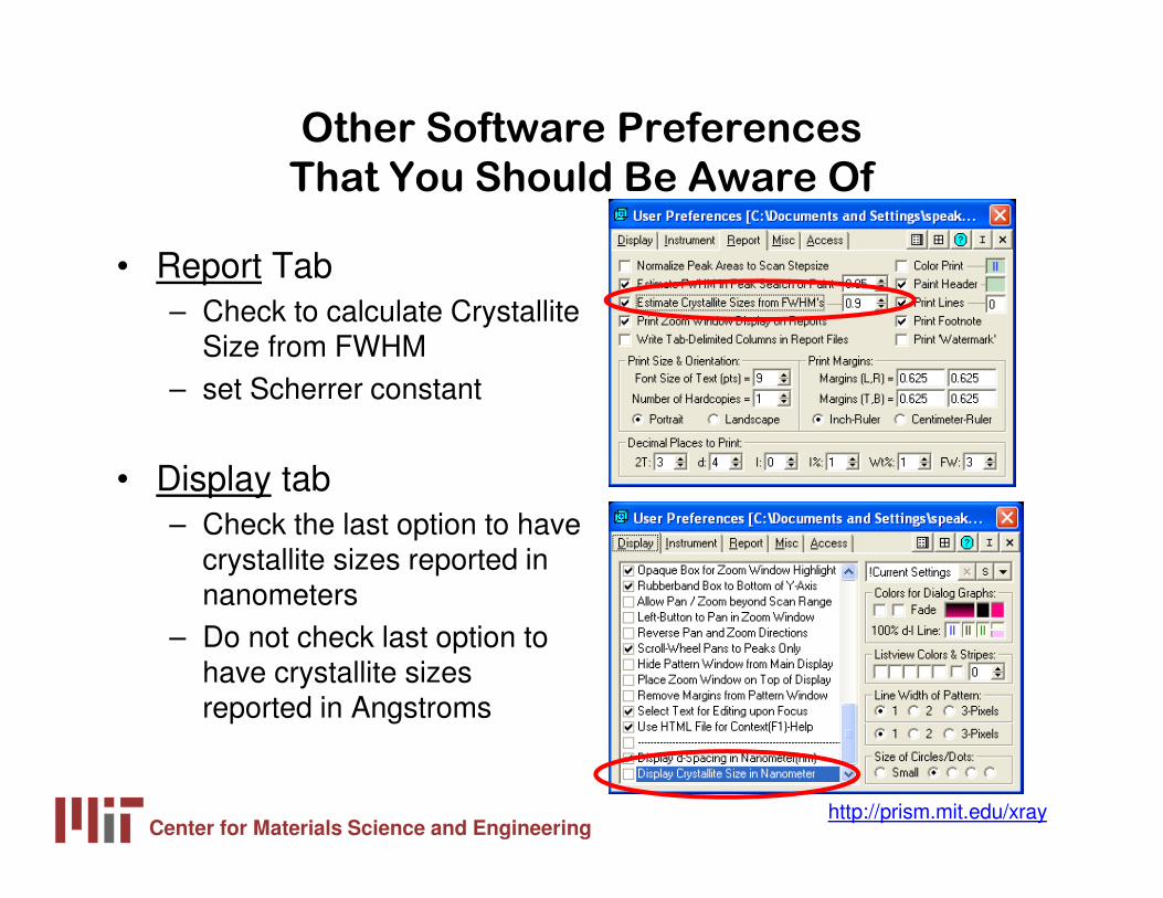
Other Software Preferences
That You Should Be Aware Of
• Report Tab– Check to calculate Crystallite
Size from FWHM– set Scherrer constant
• Display tab– Check the last option to have
crystallite sizes reported in nanometers
– Do not check last option to have crystallite sizes reported in Angstroms
Center for Materials Science and Engineeringhttp://prism.mit.edu/xray
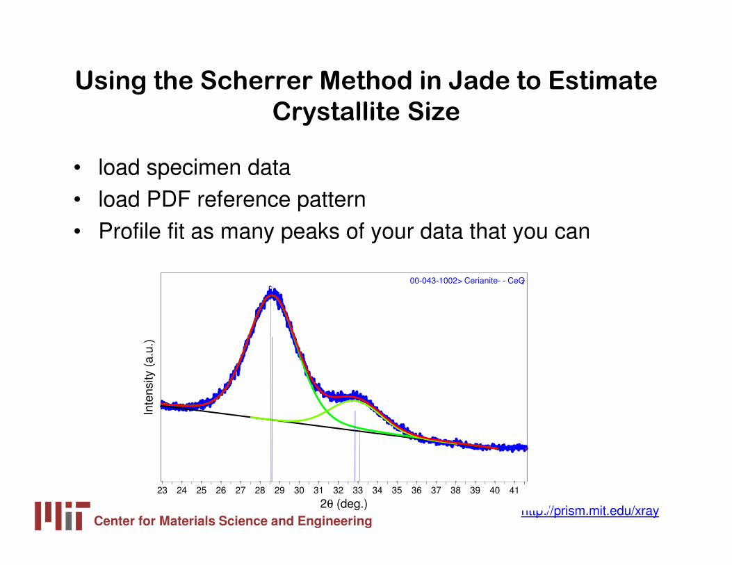
Using the Scherrer Method in Jade to Estimate
Crystallite Size
• load specimen data• load PDF reference pattern• Profile fit as many peaks of your data that you can
23 24 25 26 27 28 29 30 31 32 33 34 35 36 37 38 39 40 41
2θ (deg.)
Inte
nsity
(a.
u.)
00-043-1002> Cerianite- - CeO2

Center for Materials Science and Engineeringhttp://prism.mit.edu/xray
Scherrer Analysis Calculates Crystallite Size
based on each Individual Peak Profile
• Crystallite Size varies from 22 to 30 Å over the range of 28.5 to 95.4° 2θ
– Average size: 25 Å– Standard Deviation: 3.4 Å
• Pretty good analysis• Not much indicator of
crystallite strain• We might use a single
peak in future analyses, rather than all 8

Center for Materials Science and Engineeringhttp://prism.mit.edu/xray
FWHM vs Integral Breadth
• Using FWHM: 25.1 Å (3.4)• Using Breadth: 22.5 Å (3.7)• Breadth not as accurate because there is a lot of overlap between peaks-
cannot determine where tail intensity ends and background begins
Center for Materials Science and Engineeringhttp://prism.mit.edu/xray
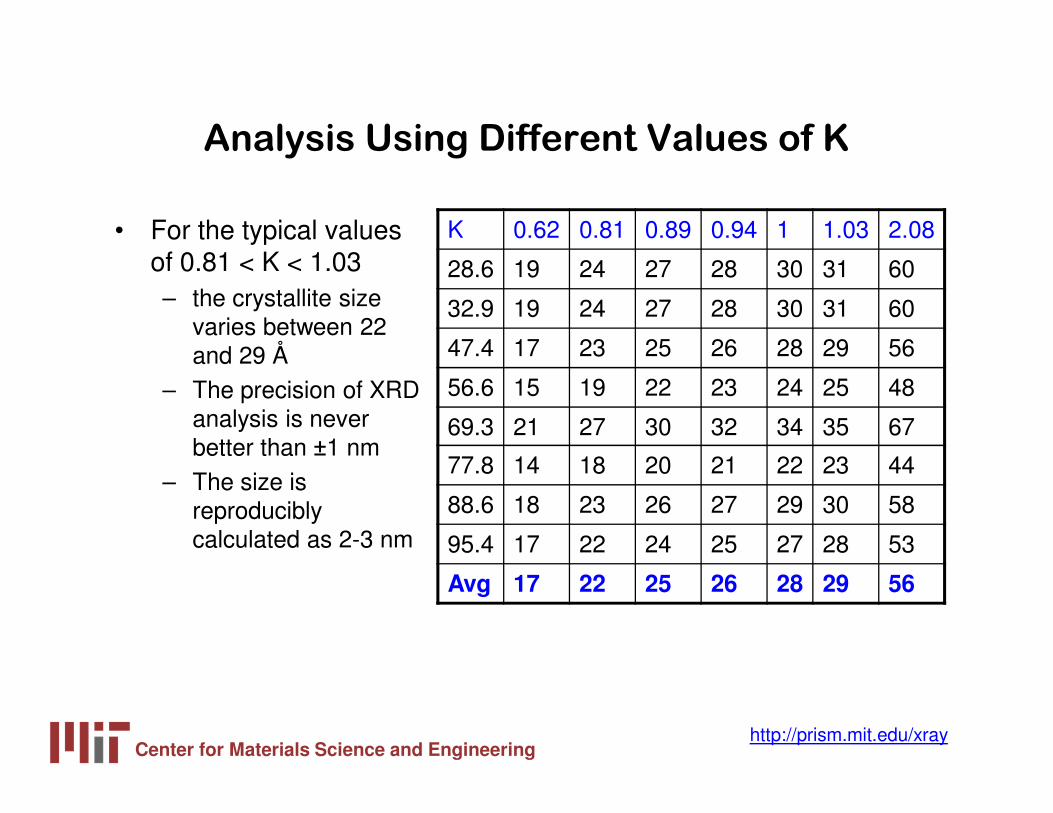
Analysis Using Different Values of K
• For the typical values of 0.81 < K < 1.03– the crystallite size
varies between 22 and 29 Å
– The precision of XRD analysis is never better than ±1 nm
– The size is reproducibly calculated as 2-3 nm
K 0.62 0.81 0.89 0.94 1 1.03 2.08
28.6 19 24 27 28 30 31 60
32.9 19 24 27 28 30 31 60
47.4 17 23 25 26 28 29 56
56.6 15 19 22 23 24 25 48
69.3 21 27 30 32 34 35 67
77.8 14 18 20 21 22 23 44
88.6 18 23 26 27 29 30 58
95.4 17 22 24 25 27 28 53
Avg 17 22 25 26 28 29 56
Center for Materials Science and Engineeringhttp://prism.mit.edu/xray
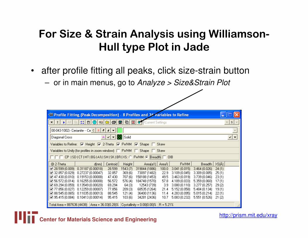
For Size & Strain Analysis using Williamson-
Hull type Plot in Jade
• after profile fitting all peaks, click size-strain button – or in main menus, go to Analyze > Size&Strain Plot
Center for Materials Science and Engineeringhttp://prism.mit.edu/xray
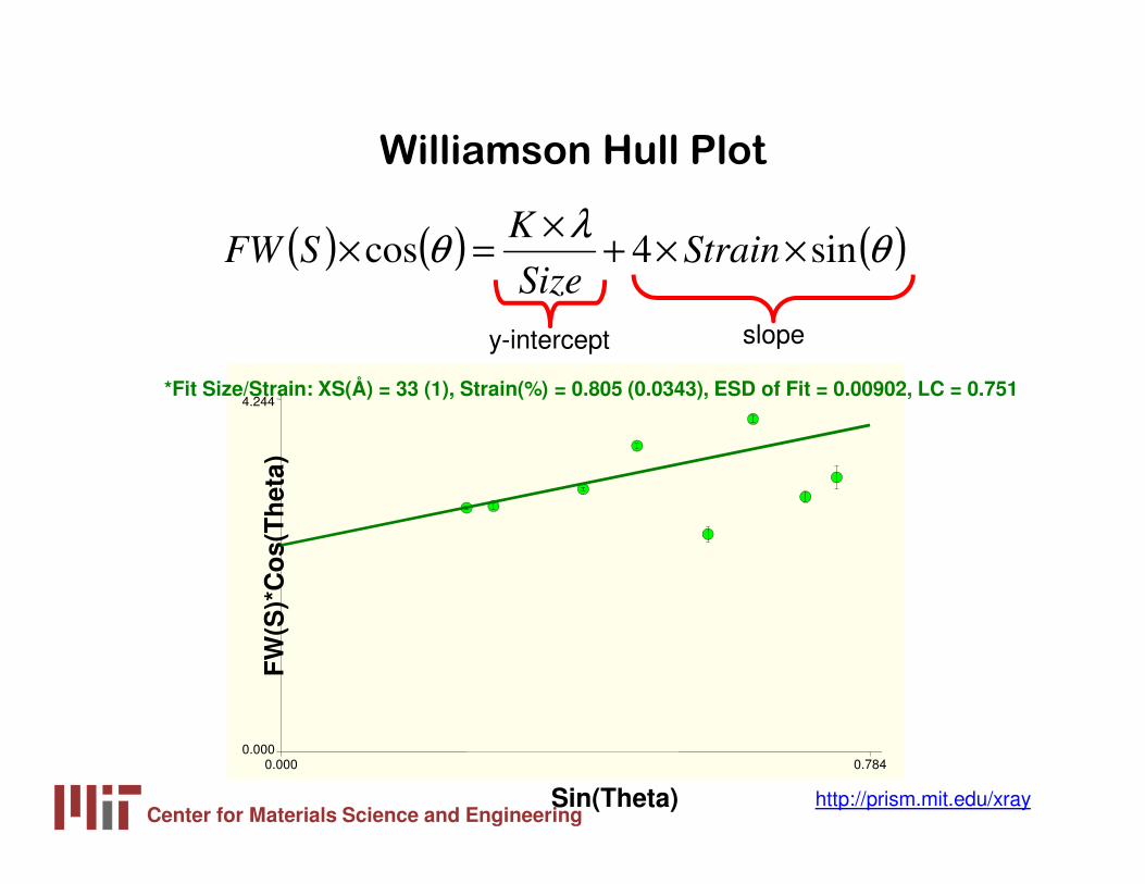
Williamson Hull Plot
( ) ( ) ( )θλ
θ sin4cos ××+×
=× StrainSize
KSFW
y-intercept slope
FW
(S)*
Co
s(T
het
a)
Sin(Theta)
0.000 0.7840.000
4.244*Fit Size/Strain: XS(Å) = 33 (1), Strain(%) = 0.805 (0.0343), ESD of Fit = 0.00902, LC = 0.751
Center for Materials Science and Engineeringhttp://prism.mit.edu/xray
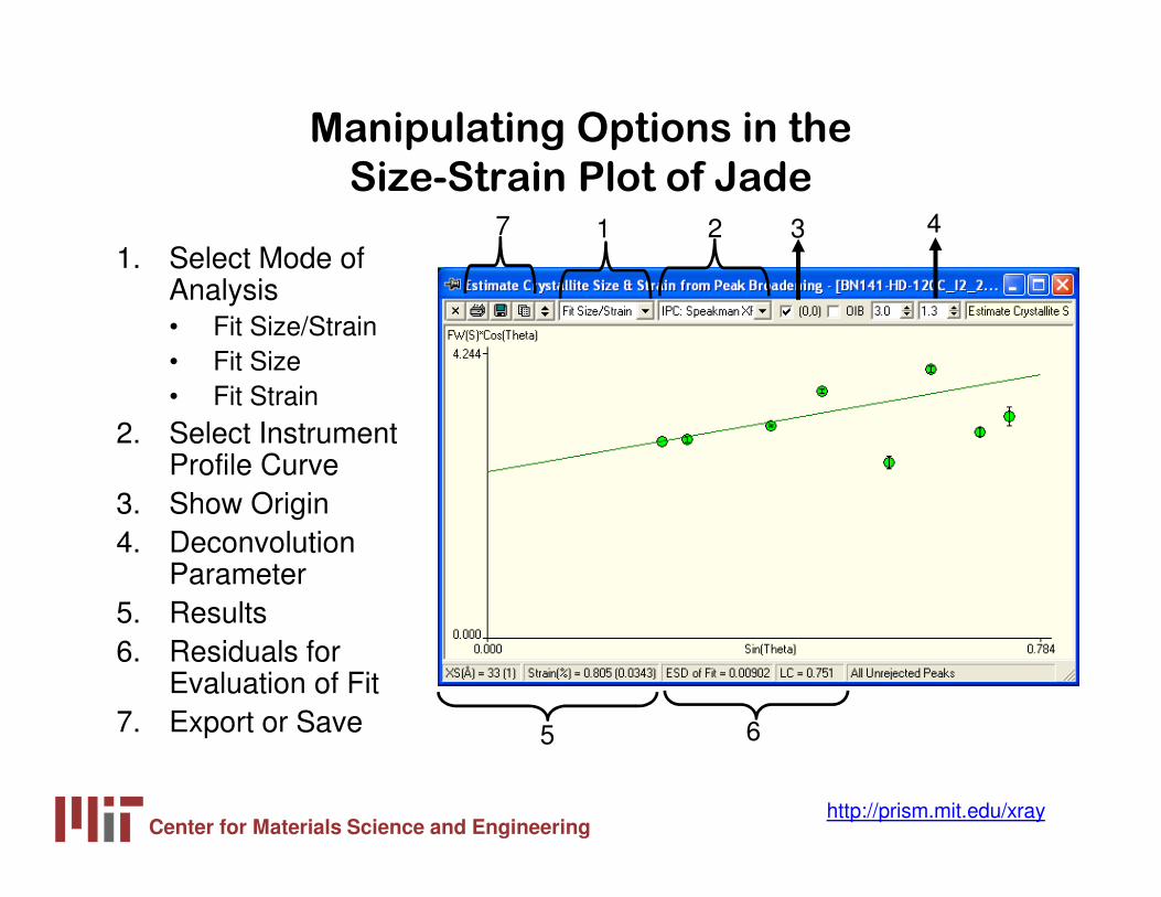
Manipulating Options in the
Size-Strain Plot of Jade
1. Select Mode of Analysis• Fit Size/Strain• Fit Size• Fit Strain
2. Select Instrument Profile Curve
3. Show Origin4. Deconvolution
Parameter5. Results6. Residuals for
Evaluation of Fit7. Export or Save
1 2 3 4
5 6
7
Center for Materials Science and Engineeringhttp://prism.mit.edu/xray
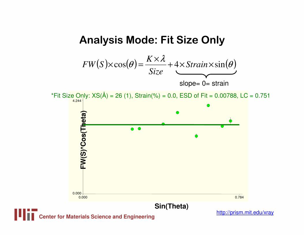
Analysis Mode: Fit Size Only
( ) ( ) ( )θλ
θ sin4cos ××+×
=× StrainSize
KSFW
slope= 0= strainF
W(S
)*C
os(
Th
eta)
Sin(Theta)
0.000 0.7840.000
4.244*Fit Size Only: XS(Å) = 26 (1), Strain(%) = 0.0, ESD of Fit = 0.00788, LC = 0.751
Center for Materials Science and Engineeringhttp://prism.mit.edu/xray
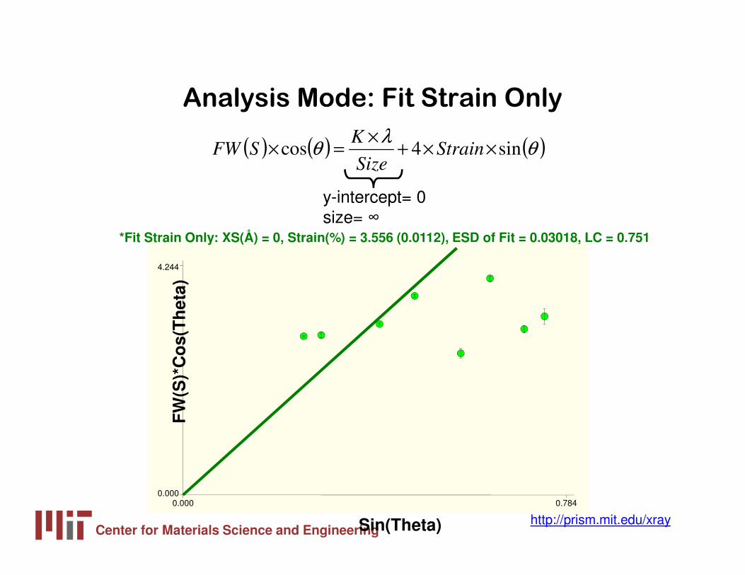
Analysis Mode: Fit Strain Only
( ) ( ) ( )θλ
θ sin4cos ××+×
=× StrainSize
KSFW
y-intercept= 0 size= ∞
FW
(S)*
Co
s(T
het
a)
Sin(Theta)
0.000 0.7840.000
4.244
*Fit Strain Only: XS(Å) = 0, Strain(%) = 3.556 (0.0112), ESD of Fit = 0.03018, LC = 0.751

Center for Materials Science and Engineeringhttp://prism.mit.edu/xray
Analysis Mode: Fit Size/Strain
( ) ( ) ( )θλ
θ sin4cos ××+×
=× StrainSize
KSFW
FW
(S)*
Co
s(T
het
a)
Sin(Theta)
0.000 0.7840.000
4.244*Fit Size/Strain: XS(Å) = 33 (1), Strain(%) = 0.805 (0.0343), ESD of Fit = 0.00902, LC = 0.751

Center for Materials Science and Engineeringhttp://prism.mit.edu/xray
Comparing Results
Size (A) Strain (%) ESD of Fit
Size(A) Strain(%) ESD of Fit
Size Only
22(1) - 0.0111 25(1) 0.0082
Strain Only
- 4.03(1) 0.0351 3.56(1) 0.0301
Size & Strain
28(1) 0.935(35) 0.0125 32(1) 0.799(35) 0.0092
Avg from Scherrer Analysis
22.5 25.1
Integral Breadth FWHM
Center for Materials Science and Engineeringhttp://prism.mit.edu/xray
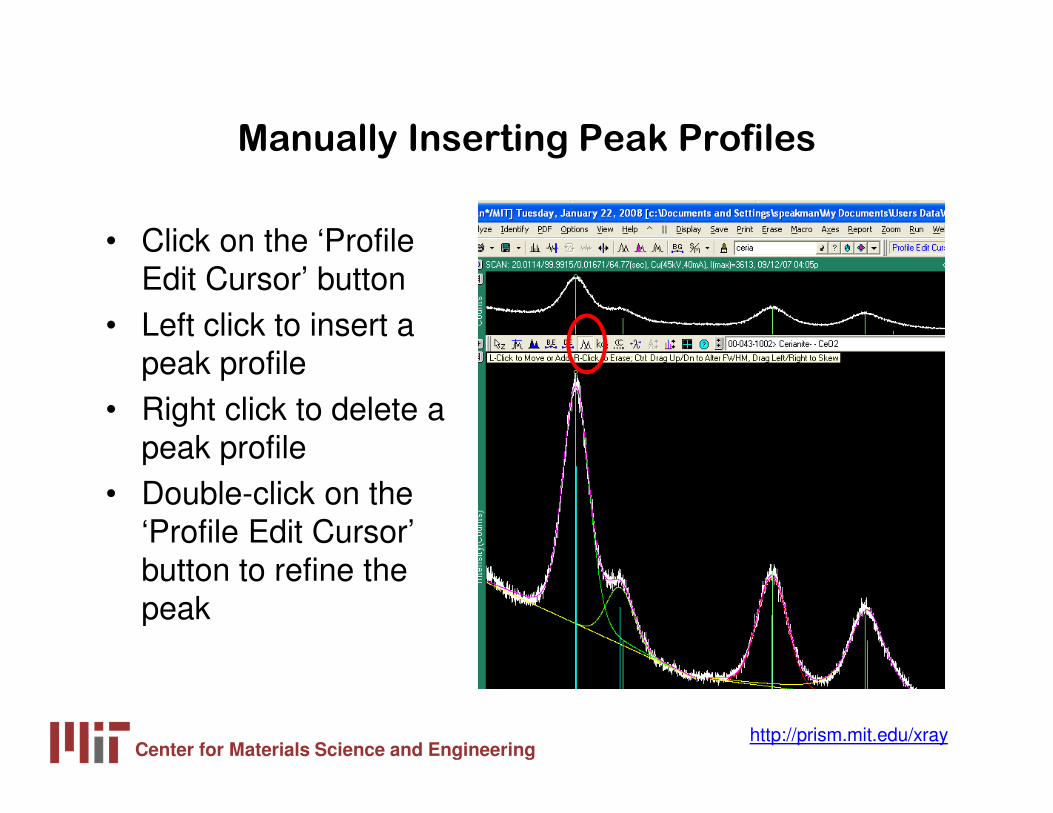
Manually Inserting Peak Profiles
• Click on the ‘Profile Edit Cursor’ button
• Left click to insert a peak profile
• Right click to delete a peak profile
• Double-click on the ‘Profile Edit Cursor’ button to refine the peak
Center for Materials Science and Engineeringhttp://prism.mit.edu/xray
Examples
• Read Y2O3 on ZBH Fast Scan.sav– make sure instrument profile is “IAP XPert FineOptics ZBH”– Note scatter of data– Note larger average crystallite size requiring good calibration– data took 1.5 hrs to collect over range 15 to 146° 2θ– could only profile fit data up to 90° 2θ; intensities were too low after that
• Read Y2O3 on ZBH long scan.sav– make sure instrument profile is “IAP XPert FineOptics ZBH”– compare Scherrer and Size-Strain Plot– Note scatter of data in Size-Strain Plot– data took 14 hrs to collect over range of 15 to 130° 2θ– size is 56 nm, strain is 0.39%
• by comparison, CeO2 with crystallite size of 3 nm took 41min to collect data from 20 to 100° 2θ for high quality analysis
Center for Materials Science and Engineeringhttp://prism.mit.edu/xray
Examples
• Load CeO2/BN*.xrdml• Overlay PDF card 34-0394
– shift in peak position because of thermal expansion
• make sure instrument profile is “IAP XPert FineOptics ZBH”
• look at patterns in 3D view• Scans collected every 1min as sample annealed in situ
at 500°C• manually insert peak profile• use batch mode to fit peak• in minutes have record of crystallite size vs time
Center for Materials Science and Engineeringhttp://prism.mit.edu/xray
Examples
• Size analysis of Si core in SiO2 shell– read Si_nodule.sav– make sure instrument profile is “IAP Rigaku RHS”– show how we can link peaks to specific phases– show how Si broadening is due completely to microstrain– ZnO is a NIST SRM, for which we know the crystallite size is
between 201 nm• we estimate 179 nm- shows error at large crystallite sizes

Center for Materials Science and Engineeringhttp://prism.mit.edu/xray
We can empirically calculate nanocrystalline
diffraction pattern using Jade
1. Load PDF reference card2. go to Analyze > Simulate Pattern
3. In Pattern Simulation dialogue box1. set instrumental profile curve2. set crystallite size & lattice strain3. check fold (convolute) with
instrument profile
4. Click on ‘Clear Existing Display and Create New Pattern’
5. or Click on ‘Overlay Simulated Pattern’
demonstrate with card 46-1212observe peak overlap at 36° 2θ as peak broaden
Whole Pattern FittingWhole Pattern FittingWhole Pattern FittingWhole Pattern Fitting

Center for Materials Science and Engineeringhttp://prism.mit.edu/xray
Emperical Profile Fitting is sometimes difficult
• overlapping peaks• a mixture of nanocrystalline phases• a mixture of nanocrystalline and macrocrystalline phase
20 30 40 50 60
2θ (deg.)
Inte
nsity
(a.
u.)
00-008-0459> Cadmoselite - CdSe
Center for Materials Science and Engineeringhttp://prism.mit.edu/xray
Or we want to learn more information about
sample
• quantitative phase analysis– how much of each phase is present in a mixture
• lattice parameter refinement– nanophase materials often have different lattice parameters from
their bulk counterparts
• atomic occupancy refinement
Center for Materials Science and Engineeringhttp://prism.mit.edu/xray
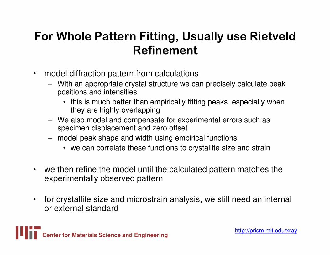
For Whole Pattern Fitting, Usually use Rietveld
Refinement
• model diffraction pattern from calculations– With an appropriate crystal structure we can precisely calculate peak
positions and intensities• this is much better than empirically fitting peaks, especially when
they are highly overlapping– We also model and compensate for experimental errors such as
specimen displacement and zero offset– model peak shape and width using empirical functions
• we can correlate these functions to crystallite size and strain
• we then refine the model until the calculated pattern matches the experimentally observed pattern
• for crystallite size and microstrain analysis, we still need an internal or external standard
Center for Materials Science and Engineeringhttp://prism.mit.edu/xray
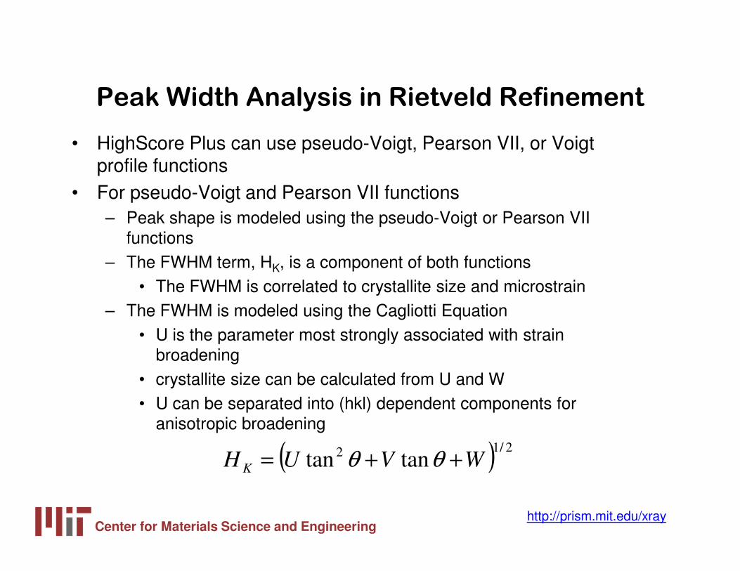
Peak Width Analysis in Rietveld Refinement
• HighScore Plus can use pseudo-Voigt, Pearson VII, or Voigt profile functions
• For pseudo-Voigt and Pearson VII functions– Peak shape is modeled using the pseudo-Voigt or Pearson VII
functions– The FWHM term, HK, is a component of both functions
• The FWHM is correlated to crystallite size and microstrain– The FWHM is modeled using the Cagliotti Equation
• U is the parameter most strongly associated with strain broadening
• crystallite size can be calculated from U and W• U can be separated into (hkl) dependent components for
anisotropic broadening
( ) 2/12 tantan WVUH K ++= θθ
Center for Materials Science and Engineeringhttp://prism.mit.edu/xray
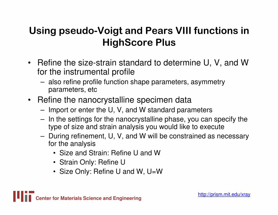
Using pseudo-Voigt and Pears VIII functions in
HighScore Plus
• Refine the size-strain standard to determine U, V, and W for the instrumental profile– also refine profile function shape parameters, asymmetry
parameters, etc
• Refine the nanocrystalline specimen data– Import or enter the U, V, and W standard parameters– In the settings for the nanocrystalline phase, you can specify the
type of size and strain analysis you would like to execute– During refinement, U, V, and W will be constrained as necessary
for the analysis• Size and Strain: Refine U and W• Strain Only: Refine U• Size Only: Refine U and W, U=W
Center for Materials Science and Engineeringhttp://prism.mit.edu/xray
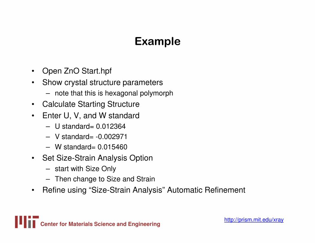
Example
• Open ZnO Start.hpf• Show crystal structure parameters
– note that this is hexagonal polymorph
• Calculate Starting Structure• Enter U, V, and W standard
– U standard= 0.012364– V standard= -0.002971– W standard= 0.015460
• Set Size-Strain Analysis Option– start with Size Only– Then change to Size and Strain
• Refine using “Size-Strain Analysis” Automatic Refinement
Center for Materials Science and Engineeringhttp://prism.mit.edu/xray
The Voigt profile function is applicable mostly
to neutron diffraction data
• Using the Voigt profile function may tries to fit the Gaussian and Lorentzian components separately, and then convolutes them– correlate the Gaussian component to microstrain
• use a Cagliotti function to model the FWHM profile of the Gaussian component of the profile function
– correlate the Lorentzian component to crystallite size• use a separate function to model the FWHM profile of the
Lorentzian component of the profile function
• This refinement mode is slower, less stable, and typically applies to neutron diffraction data only– the instrumental profile in neutron diffraction is almost purely
Gaussian

Center for Materials Science and Engineeringhttp://prism.mit.edu/xray
HighScore Plus Workshop
• Jan 29 and 30 (next Tues and Wed)– from 1 to 5 pm both days
• Space is limited: register by tomorrow (Jan 25)– preferable if you have your own laptop
• Must be a trained independent user of the X-Ray SEF, familiar with XRD theory, basic crystallography, and basic XRD data analysis
Center for Materials Science and Engineeringhttp://prism.mit.edu/xray
Free Software
• Empirical Peak Fitting– XFit– WinFit
• couples with Fourya for Line Profile Fourier Analysis– Shadow
• couples with Breadth for Integral Breadth Analysis– PowderX– FIT
• succeeded by PROFILE• Whole Pattern Fitting
– GSAS– Fullprof– Reitan
• All of these are available to download from http://www.ccp14.ac.uk
Center for Materials Science and Engineeringhttp://prism.mit.edu/xray
Other Ways of XRD Analysis
• Most alternative XRD crystallite size analyses use the Fourier transform of the diffraction pattern
• Variance Method– Warren Averbach analysis- Fourier transform of raw data– Convolution Profile Fitting Method- Fourier transform of Voigt profile
function• Whole Pattern Fitting in Fourier Space
– Whole Powder Pattern Modeling- Matteo Leoni and Paolo Scardi– Directly model all of the contributions to the diffraction pattern– each peak is synthesized in reciprocal space from it Fourier transform
• for any broadening source, the corresponding Fourier transform can be calculated
• Fundamental Parameters Profile Fitting– combine with profile fitting, variance, or whole pattern fitting techniques– instead of deconvoluting empirically determined instrumental profile, use
fundamental parameters to calculate instrumental and specimen profiles
Center for Materials Science and Engineeringhttp://prism.mit.edu/xray
Complementary Analyses
• TEM– precise information about a small volume of sample– can discern crystallite shape as well as size
• PDF (Pair Distribution Function) Analysis of X-Ray Scattering
• Small Angle X-ray Scattering (SAXS)
• Raman
• AFM
• Particle Size Analysis– while particles may easily be larger than your crystallites, we know that
the crystallites will never be larger than your particles
Center for Materials Science and Engineeringhttp://prism.mit.edu/xray
Textbook References
• HP Klug and LE Alexander, X-Ray Diffraction Procedures for Polycrystalline and Amorphous Materials, 2nd edition, John Wiley & Sons, 1974.– Chapter 9: Crystallite Size and Lattice Strains from Line Broadening
• BE Warren, X-Ray Diffraction, Addison-Wesley, 1969– reprinted in 1990 by Dover Publications– Chapter 13: Diffraction by Imperfect Crystals
• DL Bish and JE Post (eds), Reviews in Mineralogy vol 20: Modern Powder Diffraction, Mineralogical Society of America, 1989.– Chapter 6: Diffraction by Small and Disordered Crystals, by RC
Reynolds, Jr.– Chapter 8: Profile Fitting of Powder Diffraction Patterns, by SA Howard
and KD Preston• A. Guinier, X-Ray Diffraction in Crystals, Imperfect Crystals, and
Amorphous Bodies, Dunod, 1956.– reprinted in 1994 by Dover Publications
Center for Materials Science and Engineeringhttp://prism.mit.edu/xray
Articles
• D. Balzar, N. Audebrand, M. Daymond, A. Fitch, A. Hewat, J.I. Langford, A. Le Bail, D. Louër, O. Masson, C.N. McCowan, N.C. Popa, P.W. Stephens, B. Toby, “Size-Strain Line-Broadening Analysis of the Ceria Round-Robin Sample”, Journal of Applied Crystallography 37 (2004) 911-924
• S Enzo, G Fagherazzi, A Benedetti, S Polizzi, – “A Profile-Fitting Procedure for Analysis of Broadened X-ray Diffraction Peaks: I.
Methodology,” J. Appl. Cryst. (1988) 21, 536-542.– “A Profile-Fitting Procedure for Analysis of Broadened X-ray Diffraction Peaks. II. Application
and Discussion of the Methodology” J. Appl. Cryst. (1988) 21, 543-549• B Marinkovic, R de Avillez, A Saavedra, FCR Assunção, “A Comparison between the
Warren-Averbach Method and Alternate Methods for X-Ray Diffraction Microstructure Analysis of Polycrystalline Specimens”, Materials Research 4 (2) 71-76, 2001.
• D Lou, N Audebrand, “Profile Fitting and Diffraction Line-Broadening Analysis,” Advances in X-ray Diffraction 41, 1997.
• A Leineweber, EJ Mittemeijer, “Anisotropic microstrain broadening due to compositional inhomogeneities and its parametrisation”, Z. Kristallogr. Suppl. 23(2006) 117-122
• BR York, “New X-ray Diffraction Line Profile Function Based on Crystallite Size and Strain Distributions Determined from Mean Field Theory and Statistical Mechanics”, Advances in X-ray Diffraction 41, 1997.
Center for Materials Science and Engineeringhttp://prism.mit.edu/xray
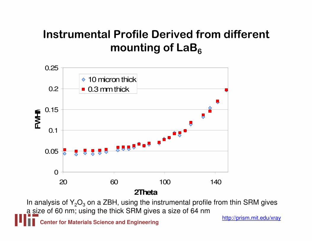
Instrumental Profile Derived from different
mounting of LaB6
0
0.05
0.1
0.15
0.2
0.25
20 60 100 140
2Theta
FW
HM
10 micron thick0.3 mm thick
In analysis of Y2O3 on a ZBH, using the instrumental profile from thin SRM gives a size of 60 nm; using the thick SRM gives a size of 64 nm


![[PPT]Estimating Crystallite Size Using XRD - Newcastle … · Web viewWhile I have tried to cite all references, I may have missed some– these slides were prepared for an informal](https://static.fdocuments.net/doc/165x107/5af9845a7f8b9a5f588e2ed7/pptestimating-crystallite-size-using-xrd-newcastle-viewwhile-i-have-tried.jpg)
![IJNEAM 4 2 6 121-134 No. 2 2011...Int. J. Nanoelectronics and tvlaterials 4 (2011) 121-134 The crystallite size, CS, can be calculated from (XRD) pattern using Scherrer formula [24].](https://static.fdocuments.net/doc/165x107/60e481e11fa46d2de3457627/ijneam-4-2-6-121-134-no-2-2011-int-j-nanoelectronics-and-tvlaterials-4-2011.jpg)


