Washington University in St. LouisWashington University Open Scholarship

Arts & Sciences Electronic Theses and Dissertations Arts & Sciences

Spring 5-15-2018

Essays on Financial and Monetary EconomicsXi WangWashington University in St. Louis

Follow this and additional works at: https://openscholarship.wustl.edu/art_sci_etds

Part of the Economic History Commons, and the Finance and Financial Management Commons

This Dissertation is brought to you for free and open access by the Arts & Sciences at Washington University Open Scholarship. It has been acceptedfor inclusion in Arts & Sciences Electronic Theses and Dissertations by an authorized administrator of Washington University Open Scholarship. Formore information, please contact digital@wumail.wustl.edu.

Recommended CitationWang, Xi, "Essays on Financial and Monetary Economics" (2018). Arts & Sciences Electronic Theses and Dissertations. 1597.https://openscholarship.wustl.edu/art_sci_etds/1597

WASHINGTON UNIVERSITY IN ST. LOUIS

Department of Economics

Dissertation Examination Committee:Costas Azariadis, Chair

Gaetano AntinolfiMichele Boldrin

Werner PlobergerNgoc-Khanh Tran

Essays on Financial and Monetary Economicsby

Xi Wang

A dissertation presented toThe Graduate School

of Washington University inpartial fulfillment of the

requirements for the degreeof Doctor of Philosophy

May 2018St. Louis, Missouri

Manjushri

c©2018, Xi Wang

Table of Contents

List of Figures . . . . . . . . . . . . . . . . . . . . . . . . . . . . . . iv

List of Tables. . . . . . . . . . . . . . . . . . . . . . . . . . . . . . . vi

Acknowledgements . . . . . . . . . . . . . . . . . . . . . . . . . . . . vii

Abstract . . . . . . . . . . . . . . . . . . . . . . . . . . . . . . . . . viii

Chapter 1 Quality Consumption and Asset Pricing . . . . . . . . . . . . 1

1.1 Introduction . . . . . . . . . . . . . . . . . . . . . . . . . . . . . . . . . . . . 21.2 Literature Review . . . . . . . . . . . . . . . . . . . . . . . . . . . . . . . . . 51.3 A parsimonious setup with general preference specification . . . . . . . . . . 131.4 Estimate the RRA with Aggregate Data . . . . . . . . . . . . . . . . . . . . 201.5 Motivation Evidence: Limited Participation in the Stock Market . . . . . . . 231.6 A Quantitative Exercise . . . . . . . . . . . . . . . . . . . . . . . . . . . . . 261.7 Data . . . . . . . . . . . . . . . . . . . . . . . . . . . . . . . . . . . . . . . . 29

1.7.1 Synthetic Consumption by the Rich, Backed from Wealth and IncomeData . . . . . . . . . . . . . . . . . . . . . . . . . . . . . . . . . . . . 32

1.7.2 Quality Goods and Equity Premium . . . . . . . . . . . . . . . . . . 341.8 More Moment Conditions . . . . . . . . . . . . . . . . . . . . . . . . . . . . 411.9 Cross-Sectional Expected Return . . . . . . . . . . . . . . . . . . . . . . . . 421.10 Conclusion . . . . . . . . . . . . . . . . . . . . . . . . . . . . . . . . . . . . . 461.11 Appendix . . . . . . . . . . . . . . . . . . . . . . . . . . . . . . . . . . . . . 47

1.11.1 An Empirical Estimation for Habit Formating Framework . . . . . . 471.11.2 Numerical Algorithm: Policy Iteration . . . . . . . . . . . . . . . . . 481.11.3 More Statistical Tables . . . . . . . . . . . . . . . . . . . . . . . . . . 52

Chapter 2 Reassessing the Quantity Theory of Money. . . . . . . . . . . 55

2.1 Introduction . . . . . . . . . . . . . . . . . . . . . . . . . . . . . . . . . . . . 552.2 Empirical Method . . . . . . . . . . . . . . . . . . . . . . . . . . . . . . . . . 672.3 Empirical Results . . . . . . . . . . . . . . . . . . . . . . . . . . . . . . . . . 72

2.3.1 Data . . . . . . . . . . . . . . . . . . . . . . . . . . . . . . . . . . . . 722.3.2 Scatter Graphs: Frequency Approach . . . . . . . . . . . . . . . . . . 73

ii

2.3.3 Evidence from Cointegration test: Temporal Approach . . . . . . . . 752.3.4 Cross countries Robust Check . . . . . . . . . . . . . . . . . . . . . . 76

2.4 Proposed Channel: Endogenous generated money and financial innovation . 772.4.1 Model outline . . . . . . . . . . . . . . . . . . . . . . . . . . . . . . . 81

2.5 Endogenous Money Creation: Loan Issuing . . . . . . . . . . . . . . . . . . . 922.5.1 Numerical Algorithm and Calibration . . . . . . . . . . . . . . . . . . 96

2.6 Conclusion . . . . . . . . . . . . . . . . . . . . . . . . . . . . . . . . . . . . . 1012.7 Appendix . . . . . . . . . . . . . . . . . . . . . . . . . . . . . . . . . . . . . 103

2.7.1 Data source, Cross-Country . . . . . . . . . . . . . . . . . . . . . . . 1032.7.2 Numerical Solution . . . . . . . . . . . . . . . . . . . . . . . . . . . . 107

Chapter 3 Quantity Theory of Money is not a Universal Rule: Evidencefrom Monetary History of Thirteen Countries . . . . . . . . . 113

3.1 Introduction . . . . . . . . . . . . . . . . . . . . . . . . . . . . . . . . . . . . 1133.2 Empirical Method . . . . . . . . . . . . . . . . . . . . . . . . . . . . . . . . . 1183.3 Empirical Results . . . . . . . . . . . . . . . . . . . . . . . . . . . . . . . . . 120

3.3.1 U.S.A . . . . . . . . . . . . . . . . . . . . . . . . . . . . . . . . . . . 1213.3.2 Australia . . . . . . . . . . . . . . . . . . . . . . . . . . . . . . . . . . 1233.3.3 Canada . . . . . . . . . . . . . . . . . . . . . . . . . . . . . . . . . . 1253.3.4 Switzerland . . . . . . . . . . . . . . . . . . . . . . . . . . . . . . . . 1263.3.5 U.K . . . . . . . . . . . . . . . . . . . . . . . . . . . . . . . . . . . . 1273.3.6 Germany . . . . . . . . . . . . . . . . . . . . . . . . . . . . . . . . . . 1293.3.7 Italy . . . . . . . . . . . . . . . . . . . . . . . . . . . . . . . . . . . . 1303.3.8 Spain . . . . . . . . . . . . . . . . . . . . . . . . . . . . . . . . . . . . 1323.3.9 France . . . . . . . . . . . . . . . . . . . . . . . . . . . . . . . . . . . 1333.3.10 Denmark . . . . . . . . . . . . . . . . . . . . . . . . . . . . . . . . . . 1353.3.11 Netherlands . . . . . . . . . . . . . . . . . . . . . . . . . . . . . . . . 1363.3.12 Norway . . . . . . . . . . . . . . . . . . . . . . . . . . . . . . . . . . 1373.3.13 Sweden . . . . . . . . . . . . . . . . . . . . . . . . . . . . . . . . . . 139

3.4 Conclusion . . . . . . . . . . . . . . . . . . . . . . . . . . . . . . . . . . . . . 140

Bibliography . . . . . . . . . . . . . . . . . . . . . . . . . . . . . . . 141

iii

List of Figures

1.1 Equity held by Top 10% wealthy, annual data, source:Piketty, Saez and Zuc-man (2016) . . . . . . . . . . . . . . . . . . . . . . . . . . . . . . . . . . . . 26

1.2 Implied Risk aversion Coefficient by backed-consumption of rich . . . . . . . 28

1.3 Synthetic Consumption of the Rich and Excess Return, 1945-2012, Annual Data 32

1.4 Luxury sales and Excess Return, 1962-2015, Annual Data . . . . . . . . . . . 34

1.5 Premium Grocery sales and Excess Return . . . . . . . . . . . . . . . . . . . 35

1.6 Luxury Lodging and Excess Return . . . . . . . . . . . . . . . . . . . . . . . 37

1.7 Index of Stock of Quality Goods and Excess Return . . . . . . . . . . . . . . 38

1.8 CCAPM can explain almost nothing cross-sectionally . . . . . . . . . . . . . 40

1.9 1927-2012, Realized versus predicted excess returns(25 Portfolio), Top Con-sumption . . . . . . . . . . . . . . . . . . . . . . . . . . . . . . . . . . . . . . 40

1.10 1927-2012, Realized versus predicted excess returns(100 Portfolio), Top Con-sumption . . . . . . . . . . . . . . . . . . . . . . . . . . . . . . . . . . . . . . 43

1.11 Realized versus predicted excess returns(25 Portfolio) . . . . . . . . . . . . . 44

1.12 Realized versus predicted excess returns(100 Portfolio) . . . . . . . . . . . . 45

2.1 Does Price of Final Goods Follow any Money index? Source: H.6 Money StockMeasure table provided by the Federal Reserve Board, 1959-2016, Annual data 57

2.2 Does Price of Final Goods Follow any Money index? Source: H.6 Money StockMeasure table provided by the Federal Reserve Board, 1959-2016, Annual data 58

2.3 Gain function of different filter specification . . . . . . . . . . . . . . . . . . 66

2.4 Growth rate of Money stock against Inflation rate and Real GDP, U.S . . . . 70

2.5 Filtered Growth rate of Money stock against Inflation rate, 1955-2006, U.S . 72

2.6 Ratio of (New) M1 over GDP against interest rate (3 month) with Lucas(1980) Exercise, Baumol-Tobin Specification, 1915-2006, Annual data . . . . 73

2.7 Candidate Cointergeration residuals, De-mean . . . . . . . . . . . . . . . . . 77

2.8 Growth of estimated M2 into Real estate and relevant inflations . . . . . . . 78

2.9 Ratio of Commercial and Industry loans and mortgage loan over total loans,all commercial banks .Source: H.8 table provided by the Federal ReserveBoard, 1945-2016, monthly data . . . . . . . . . . . . . . . . . . . . . . . . . 81

2.10 Market value of land/GDP ratio .Source: Davis and Heathcote(2007), Quar-terly data . . . . . . . . . . . . . . . . . . . . . . . . . . . . . . . . . . . . . 83

iv

2.11 (Filtered) Growth rate of Money stock against Inflation rate and Price of RealEstate, U.S . . . . . . . . . . . . . . . . . . . . . . . . . . . . . . . . . . . . 85

2.12 Ratios between consumer credit and M1(wealth), U.S, Source: G.19 and Z.1Table from Federal Reserve Board . . . . . . . . . . . . . . . . . . . . . . . . 90

2.13 Structure replacement cost over GDP, Quarterly data, 1975Q1-2016Q4, source:Davisand Heathcote (2007) . . . . . . . . . . . . . . . . . . . . . . . . . . . . . . . 92

2.14 The path of consumption, borrowing and asset price under one realizationpath of zt with simulated Belief against Financial Structure Parameters Ft 98

2.15 How do household borrow? Source: Flow-of-Funds tables provided by theFederal Reserve Board, 1945-2016, annual data . . . . . . . . . . . . . . . . . 99

2.16 Distribution of βt, 10000 simulation paths of zt . . . . . . . . . . . . . . . 1022.17 Policy functions under different Financial structure parameters realization Ft,

given y = Y H . . . . . . . . . . . . . . . . . . . . . . . . . . . . . . . . . . . 111

3.1 Filtered Growth rate of Money stock against Inflation rate, U.S . . . . . . . 1223.2 Filtered Growth rate of Money stock against Inflation rate, Australia . . . . 1243.3 Filtered Growth rate of Money stock against Inflation rate, Canada . . . . . 1253.4 Filtered Growth rate of Money stock against Inflation rate, Switzerland . . . 1263.5 Filtered Growth rate of Money stock against Inflation rate, U.K . . . . . . . 1273.6 Filtered Growth rate of Money stock against Inflation rate, Germany . . . . 1293.7 Filtered Growth rate of Money stock against Inflation rate, Italy . . . . . . . 1313.8 Filtered Growth rate of Money stock against Inflation rate, Spain . . . . . . 1323.9 Filtered Growth rate of Money stock against Inflation rate, France . . . . . . 1343.10 Filtered Growth rate of Money stock against Inflation rate, Denmark . . . . 1343.11 Filtered Growth rate of Money stock against Inflation rate, Netherlands . . . 1363.12 Filtered Growth rate of Money stock against Inflation rate, Norway . . . . . 1383.13 Filtered Growth rate of Money stock against Inflation rate, Sweden . . . . . 139

v

List of Tables

1.1 Estimated or Calibrated RRA in Previous Literature . . . . . . . . . . . . . 41.2 Risk Aversion Implied by Aggregate Data . . . . . . . . . . . . . . . . . . . 231.3 Sample Observation of Shareholder, PSID:1984-2015 . . . . . . . . . . . . . . 251.4 Risk Aversion Implied by quality goods and service data . . . . . . . . . . . 391.5 Estimated RRA with Habit formating specification . . . . . . . . . . . . . . 491.6 Sample Observation of Shareholder, PSID:1984-2015 . . . . . . . . . . . . . . 521.7 Risk Aversion Estimation with Four Moment Condition . . . . . . . . . . . . 531.8 Risk Aversion Estimation with 25 Size to Book Portfolio(Value Weight) . . . 531.9 Risk Aversion Estimation with 25 Size to Book Portfolio(Equally Weight) . . 54

2.1 Calibration Parameter . . . . . . . . . . . . . . . . . . . . . . . . . . . . . . 100

vi

Acknowledgments

I am particularly grateful to my main advisor Costas Azariadis for his inspiration, advice and

patience. I am also in debt to Michele Boldrin and Gaetano Antinolfi for their enlightening

discussion and training. I appreciate the conversation with the faculty members and students

from the Department of Economics and Finance at Washington University in St. Louis, Saint

Louis University and University of Missouri–St. Louis. Meanwhile, I really appreciate the

supports from my parents, my wife Xiao Hu and Manjushri.

Certainly, I offer special thanks to Washington University Economic Department for its

rigorous training and financial funding. Moreover, I really appreciate the patience and love

from my parents and wife.

Xi Wang

Washington University in St. Louis

May 2018

vii

ABSTRACT OF THE DISSERTATION

Essays on Financial and Monetary Economics

by

Xi Wang

Doctor of Philosophy in Economics

Washington University in St. Louis, 2018

Professor Costas Azariadis, Chair

The first part of this dissertation explores an empirical relevance to understand the

equity premium puzzle. Since only the wealthiest people invest significant amounts in the

stock market (limited participation), it is reasonable to combine the consumption data of

the wealthy, instead of aggregate data, with observed asset returns to estimate the risk

aversion coefficient (RRA). I approximate the consumption by the rich from two angles: one

explores the income and wealth data to back out synthetic consumption directly, and the

other explores the sales data to approximate the expenditure by the rich. By using the

created indices, the lowest RRA estimate is around three for the first approach, and slightly

below ten for the second one. Furthermore, when I use my indices to fit more moments

besides excess return, the estimate of RRA increases modestly, e.g., to fit returns of 25 size

and book-to-market portfolios, estimates of RRA are between 2.16 and 18. I conclude that

these indices, especially the top consumption processes, provide a useful vantage point from

which we can reassess the theory of consumption-based asset pricing. When I used these

newly constructed indices in a factor model, my factor model explains cross-sectional excess

returns better than CAPM and CCAPM model with aggregate consumption.

The latter two parts are to re-evaluate the Quantity Theory of Money(QTM) using, to

the extent possible, the same statistical and economic criteria but a much larger data set

covering both a longer period and many more countries. I investigate whether QTM breaks

viii

across countries and I find Lucas’ result fragile. It appears that the period 1955-1980 is the

only period during which QTM fits data well in most of our sample countries. It starts to

break down when we go beyond this period. Furthermore, the recent breaking down of QTM

is not global when I truncate the sample before the crisis since QTM is not a tight rule across

countries. To explain the breaking down for the U.S during Pre-crisis Period (1980-2007),

the second part shows M2 is a more robust monetary index by investigating the historical

performance of M1. Under the view of endogenous money. Namely, broad money(M2) is

generated from loan issuing. I decompose the structure of loans for the U.S. I found that real

estate is the major collateral asset for Household and Firms. I thus propose money is after

real estate and final goods. To confirm our theory, we investigate a historical nominal price

index of U.S and find that (long-run) growth of nominal house price co-moves with(leads)

growth of broad money more robustly. Furthermore, the timing of recent financial innovation

matches with breaking data. I thus propose a channel through which financial innovation

can affect the estimation of QTM.

ix

Chapter 1

Quality Consumption and Asset

Pricing

This paper explores an empirical relevance to understand the equity premium puzzle. Since

only the wealthiest people invest significant amounts in the stock market (limited participa-

tion), it is reasonable to combine the consumption data of the wealthy, instead of aggregate

data, with observed asset returns to estimate the risk aversion coefficient (RRA). I approx-

imate the consumption by the rich from two angles: one explores the income and wealth

data to back out synthetic consumption directly, and the other explores the sales data to

approximate the expenditure by the rich.

And by using the created indices, the lowest RRA estimate is around three for the first

approach, and slightly below ten for the second one. Furthermore, when I use my indices to

fit more moments besides excess return, the estimate of RRA increases modestly, e.g., to fit

returns of 25 size and book–to–market portfolios, estimates of RRA are between 2.16 and

18. I conclude that these indices, which are approximations to the consumption of the rich,

provide a useful vantage point from which we can reassess the theory of consumption-based

asset pricing. When I used these newly constructed indices in a factor model, my factor

1

model explains cross-sectional excess returns better than CAPM and CCAPM model with

aggregate consumption.

1.1 Introduction

The equity premium puzzle has been at the heart of financial economics since Mehra and

Prescott (1985) (afterward, MP). MP adopts a representative agent framework with time-

separable CRRA utility, and calibrates the model to match the average excess return of

the stock, i.e., the difference between stock market returns and risk-free rate1. It turns out

that this model requires an unreasonably high risk aversion coefficient to match the equity

premium which is annually 6% on average.

The intuition follows a general idea: people invest or save for future consumption. Assets

that offer insurance have high prices and low returns. An example is Treasury bonds or life

insurance. Contrastly, risky assets have high returns, e.g., stocks. As the old saying goes, the

greater the risk, the greater the reward. An average 6% excess return (reward) implies stock

should be a risky asset. However, when one turns to data, she will find a low co-variance2

between the consumption growth and stock return. The consumption data states that stock

is not a bad hedge against consumption risk, though the stock is still mildly risky. To justify

these two phenomena, investors should be extremely risk averse to require a high (6%) excess

return as compensation for this mild risk. In other words, the risk aversion coefficient(RRA

afterward) is high. However, the required RRA is too high to fit in any reasonable range by

any literature in other fields.

In addition, high risk aversion involves another problem: the “risk-free rate puzzle”

(Weil (1989)). High RRA implies an unreasonably high risk-free rate under the CRRA

1In this article, I use one month T-bill rate as the risk-free rate. The puzzle prevails even if one usesreturns on treasury bonds with other maturities.

2It is worth pointing out that low covariance between consumption and risky return comes from the lowvolatility of consumption data.

2

utility specification. Risk aversion has implications for peoples’ intertemporal behaviors

under the CRRA setup: the elasticity of intertemporal substitution (EIS afterward) equals

to the reciprocal of RRA. A high risk aversion means a low EIS. A representative agent with

low EIS prefers a smooth intertemporal consumption path. However, U.S consumption per

capita grows stably, not a smooth path at all. A high risk-free interest rate is thus necessary

to justify this consumption deferral. Alternatively the agent values future consumption more:

β > 1, e.g., Kocherlakota (1996).

In this paper, I provide an angle to understand this “puzzle”: to provide another empirical

relevant measure for the risk imposed by the stock. First, I present evidence of limited

participation. I show that not all Americans invest in the stock market. Only the wealthiest

invest significantly in this market, echoing the evidence in Mankiw and Zeldes (1990, 1991).

Therefore, the consumption of the rich should be the relevant consumption sequence one

should use to justify this 6% annual premium. To approximate the consumption of the

rich, I use two approaches: one explores the data from Piketty, Saez and Zucman (2016)

on the income and wealth of the rich to back out a synthetic consumption by the rich,

and the other uses sales data of luxury goods and services to approximate the expenditure

by the rich; To be more precise, I create three quality consumption indices (1960-2015) by

following the second method: U.S sales of luxury brands, sales of luxury lodging service and

sales of premium grocery. During 1960-2014, the correlation coefficient between personal

consumption expenditure and average individual income is 0.76. During the same period,

the correlation coefficient between my quality service (goods) and the average income of the

top 10% of the rich is 0.630 (0.368).

By using these indices, I reestimate RRA under an endowment economy with the CRRA

preference. Estimates are much lower than the ones in the previous empirical literature with

a similar setup. For example, the lowest estimate of RRA is 3.8 (7.6 if using the quality

index), lower than 13.9 in Ait-sahalia, Parker and Yogo (2004), and lower than 17 in Savov

3

(2011). Previous successful literature has low calibrated RRA ranging from 1 to 10 and

above, but the most successful ones are all from the calibration side. For example, Boldrin,

Christiano and Fisher (2001) use habit formation and the log utility setup. Barro (2009)

combines rare disaster with Epstein-Zin preferences and calibrates RRA to be 3−4. Finally,

Bansal and Yaron (2004) combine Epstein-Zin preferences with long-run risk and stochastic

volatility and calibrate RRA to be 10 or above3. I summarize this comparison in Table-1.1

and leave a detailed review of the literature to next section. My estimate of RRA is the

lowest among empirical studies.

Table 1.1: Estimated or Calibrated RRA in Previous Literature

Preference Specification Additional Assumptions Calibrated RRAor Data Or Estimated

Mehra and Prescott (1985) CRRA n.a Calibrated 10Campbell and Cochrane (1999) CRRA Habit Formation Calibrated 2a

Boldrin, Christiano and Fisher (1997) CRRA Habit Formation Calibrated 1Barro (2006) CRRA Rare Disaster Calibrated 4b

Barro (2009) E-P Rare Disaster Calibrated 3–4Bansal and Yaron (2004) E-P Persistent Consumptionc Calibrated 10

Constantinides et.al.(2002) CRRA Credit market imperfection Calibrated 6Mankiw and Zeldes (1990) CRRA Consumption of Shareholders Estimated 35

Yogo (2006) E-P Durable goods Estimated 174–206Ait-sahalia el.at.(2004) CRRA Luxury Cars and Durables Estimated 13-20

Savov (2011) CRRA Garbage Data Estimated 17Kronencke (2017) CRRA Unfilter Estimated 15.76

a However, the de facto risk aversion still range from 60 to 80 (Page 243).b With a RRA valued at 4, Barro (2006) can justify an excess return 0.16% (Page 843).c Stochastic Volatility and Large EIS are also necessary to justify a 6% equity premium. Without stochastic volatility, a

RRA valued at 10 can only justify a excess return less than 5%.

In the following sections, I will first briefly review relevant literature and link my pro-

cedure and results to that. In section III, I lay out a parsimonious model to nest several

preference specifications and to accommodate composition risks. In section IV, we use ag-

gregate data and explore Euler Equations to estimate RRA γ under different specifications.

In section V, I provide two pieces of time series evidence to show limited participation of the

stock market. In section VI, I start to create consumption indices for the rich. And RRA

will be re-estimated by using these created indices in section VII. In section VIII, I explore

3Depends on whether they include stochastic volatility or not. See following literature review for details.

4

the cross-sectional implication of my newly constructed pricing kernels. A conclusion section

will then follow.

1.2 Literature Review

Researchers try to solve the Equity Premium puzzle in various ways. solutions can be

categorized into model- and data-oriented approaches. The model approach considers more

assumptions, while the data approach investigates and explores relevant indices to price

assets, because of issues of NIPA consumption data, which we will elaborate later.

For the model approach, different researchers introduce various additional elements (as-

sumptions) into the classical Lucas-tree model. There are at least four groups of successful

and elegant literature: rare disaster, habit formation, long-run risk and imperfect credit

market.

The rare disaster model, first introduced by Rietz (1988) and further developed by Barro

(2006) and Gabaix (2012), states that there is a small but positive probability of a rare

disaster. This rare event reduces consumption significantly when it happens, e.g., 15% Barro

(2006). Though this rare event does not happen in postwar datasets which is a typical sample

period people are investigating, it did happen and this rare event is so important(significant

consumption cut) that investors cannot ignore their existence (a peso problem, as stated in

Rietz (1988)). With this tail-event, cautious investors will require a relative high return on

stock and other risky assets, though Epstein and Zin preference is still necessary to lower

the RRA to a reasonable range, e.g., Under a CRRA specification, γ = 4 can only justify

0.16% excess return (Page 843, Barro (2006)).

Epstein and Zin preference (E-Z preference afterward) is invented by Epstein and Zin

(1989). Under the E-Z preference, the RRA is separated with EIS4. Under this preference,

4see Epstein and Zin (1989, 1991) for further discussion of recursive utility

5

high risk aversion does not necessarily imply a low EIS or a high risk-free rate. However, the

E-Z preference alone cannot generate a high equity premium without the help of a high RRA.

This preference cannot deliver a reasonable answer even when one may add in composition

risks, for example, Yogo (2006)5. A high RRA is still necessary to justify 6% equity premium

even with this composition risk. With E-Z preferences, Yogo (2006) estimates RRA to be 174

to 199 (Table II, Page 552). Additional elements are thus necessary to lower the estimate.

There is another strand of models that successfully takes the advantage of the E-Z pref-

erence: the long-run risk model, e.g., the pioneering work Bansal and Yaron (2004). Under

the E-Z preferences, people care about future uncertainty, and under certain parameter re-

strictions (RRA > 1EIS

) people are willing to pay for early resolution of that uncertainty. In

other words, people need to be compensated for future risks. The required compensation

positively depends on the magnitude of risk people are facing. There are thus two indispens-

able elements to make the long-run model consistent with both a low RRA and a 6% equity

premium: (1) A persistent component6 in consumption process7. Since other components of

consumption are deterministic, any consumption shock is long-lasting, like a I(1) Process.

Hence this model is named as “long-run” risk model. (2) Stochastic Volatility; the volatil-

ity of this “long-run” risk is also random. In other words, there are two layers of future

uncertainty to resolve, if anyone can do so. When one of these two elements is absent, the

5Yogo (2006) differentiates durable goods with nondurable goods and services. The ratio between thesetwo is varying over time. Yogo (2006) names this as composition risk

6Persistent shocks may have potential surprising implications on the time-varying property of EquityPremium as pointed out in Boldrin, Christiano and Fisher (1997). Good Shock may bring negative return.The intuition goes as follows: In a life-cycle model, consumption is determined by permanent income. Ifshocks of income are signaling even higher future income, a good shock means higher permanent income,which causes higher consumption than dividends. People thus have the incentive to sell the tree. To clearasset market, the return of stock should go up and price of the stock goes down. Negative return is generated.Under a (un)carefully calibrated model, RRA can be negatively associated with implied excess return.

7However, it is hard on the basis of a finite sample of observation to test whether a process containsa persistent component or is merely a white noise; This problem is two-sided:For any given sample size(1) for a process contains a persistent component there exists a white noise process such that it is almostindistinguishable from the previous candidate.(2) for any white noise process, we can write down a processcontaining a persistent component. And this constructed process is indistinguishable from the white noise.See Shephard and Harvey (1990).

6

long run risk model cannot justify the 6% equity premium with an RRA less than 10, for

example, Table-II in Page 1492 of Bansal and Yaron (2004).

Another successful preference-based approach is offered by habit forming preference8, e.g.,

Boldrin, Christiano and Fisher (1997, 2001) and Campbell and Cochrane (1999)9. Even with

a constant risk-free interest rate and random walk consumption, this setup can generate a

large equity premium and volatile stock price. The main mechanism is through “endogenous”

risk aversion. When consumption (C) falls behind habit (X), the “endogenous” risk aversion

increases (−UcccUc

= γ CC−X ), driving up the equity premium and decreasing stock price10. But

the risk aversion coefficient is de facto high, “Risk aversion is about 80 at steady state,..., and

is still as high as 60 at the maximum surplus consumption ratio... (Campbell and Cochrane

(1999), Page 244).”

The last strand explores additional market structure, e.g., borrowing constraint11. Under

imperfect credit specification, there are at least two working channels increasing the implied

excess return, e.g., the elegant setup of Constantinides, Donaldson and Mehra (2002). (1)

Precautionary saving channel lowers the risk-free rate. One problem with CRRA utility

specification is that increasing RRA boosts risk-free rate, excess return thus increases in-

significantly, e.g., Page 842–843 Barro (2006). (2) Worsen hedging channel increases required

the return of stock directly and indirectly. When borrowing constraint binds, people want

to consume more but they cannot. There is an incentive to sell the asset. To clear the asset

8Recently, Yang (2016) tests habit formation model against long-run risk model, the former is preferred9To be more precise, one needs a special kind of habit formation preference, for example, ratio habit

formation in Abel (1990) does not work well. The habit formation here is in the form of difference.10This statement follows Campbell-Shiller decomposition. Campbell and Shiller (1988) prove that higher

expected excess return means lower current price. It is also worth pointing out that Yogo (2008) derives aframework by using reference-dependent preferences. This setup is similar to habit formation model sincehabit itself serves as a natural type of reference point. The calibrated RRA is 1 in Yogo (2008) (Page 137).

11There is also a huge literature combing incomplete market(market structure), heterogeneity with habitformation or Epstein and Zin preference to study the Equity premium. Examples are Constantinides andDuffie (1996), Heaton and Lucas (1996), Krusell and Smith (1998), Constantinides et al. (2002), Storeslettenet al. (2004), Basak and Cuoco(1998) and He et al. (1990,1991). Alvarez and Jermann(2001) and Lustiget al. (2005) use an endogenous incomplete market framework and argue that the observed distribution ofwealth justifies a 3% premium.

7

market, the return of stock has to go up.

Furthermore, there is an indirect channel: limited borrowing makes consumption smooth-

ing more difficult. Though borrowing constraint may be slack currently, risky assets, like

stock, can potentially make this constraint binding in the future, especially when there is

a collateral constraint, e.g. Wang (2017). Borrowing limit thus makes the positive co-

movement between consumption and risky return closer.

However, most of these modified models can perform well quantitatively but not empiri-

cally, since all of their critical assumptions are hard to test, Constantinides, Donaldson and

Mehra (2002) is an elegant exception, it explores the limited participation structure of the

stock market and made a realistic model specification. To be more precise: (1) Though E-P

preferences with low RRA can generate a high equity premium when the possibility of rare

disaster is added, the model suffers from sample biases. It is hard to estimate the probability

of this “rare” event out of several data points. (2) For the long-run risk model, it is hard to

test a consumption process with a persistent component against a white noise. The magni-

tude of EIS is another issue12. But the implications out of these two processes are different.

A model with white noise consumption process implies a nearly zero equity premium, while

a small but persistent component can generate a significantly higher equity premium13. (3)

For the habit formation model, we do not have direct measures or observation of “habit”

term, let alone the statistical properties of the process of this habit term14. Hence, the suc-

cess of these three models comes from quantitative exercises, instead of empirical evidence.

Additionally, rare disaster model is fragile under learning framework: Chen, Joslin and Tran

(2012) show that under heterogeneous belief setting, the rare disaster model can only deliver

12A successful calibration requires an EIS larger than 1, much higher than the number in literature focusingon estimating this parameter, e.g., EIS is estimated to be 0.4 in Chirinko and Mallick(2017). See footnote-21for more details.

13Equity premium is 4.20% without stochastic volatility for RRA=10, EIS=1.5. Table II, Page 1492,Bansal and Yaron (2004).

14It is worth mentioning that the unfiltered process in Kronencke (2017) has a similar form of habitformation, e.g., the formula in Page 54.

8

a 2% equity premium when optimists own 10% wealth of the economy.

On the other hand, the literature, using data-oriented approach, reminds us that the

aggregate consumption data released by NIPA are not satisfying ones to determine the

pricing kernel since NIPA uses filtering and interpolation methods to smooth out fluctuations

in consumption15. Therefore, the resulting pricing kernel is not volatile enough16 unless with

a high RRA. There are papers trying to address this problem by using other data sources

or modifying raw data. Parker and Julliard (2005) adopt consumption growth during a

longer horizon instead of the annual growth rate: three years consumption growth is used.

Jagannathan and Wang (2007) use fourth quarter to fourth quarter consumption growth.

Savov (2011) uses garbage data to approximate the “true consumption. As a work closet to

mine, Ait-sahalia, Parker and Yogo (2004) argues that since normal consumption is essential

to people’s lives, what is important for asset prices is non-subsistence consumption. Luxury

consumption, on the other hand, has no issues on subsistence. Ait-sahalia, Parker and

Yogo (2004) collect luxury cars, luxury brand goods, luxury housing and wine data to price

assets. More recently, Kronencke (2017) explores the implication of reversing a forward

Kalman filter, “un-filtering” the filtered consumption data17 and use the “unfiltered” data

to estimate RRA.

All these alternative (approximate) consumption processes are more volatile and corre-

lated with stock returns than the canonical measures; researchers can reduce the estimated

risk aversion into a lower range, say under 20.

In this paper, I follow another angle to understand this asset puzzles: limited participation

in the stock market. I create more comprehensive and longer quality consumption indices

to approximate the consumption of the rich. And I use these created indices to reassess the

15This contributes to the low volatility of raw consumption data.16As pointed out in Hansen and Jagannathan (1991), a nonvolatile pricing kernel generates low equity

premium.17This method only works if NIPA uses forward Kalman filter only. It cannot recover the original data if

NIPA additionally employs a Kalman smoothing process.

9

Equity Premium Puzzle.

Limited market participation refers to the fact that when not all agents in our economy

invest substantially in stocks. This pattern has more profound implication of pricing kernel:

the aggregate consumption sequence provides little evidence on the risk aversion coefficient of

the actual stock investors18, as emphasized in Brav, Constantinides and Geczy (2002). There

are theoretical papers exploring this pattern, e.g. ,iteConstantinides2002. In sum, the risk

of stock assets should be measured by its co-movement with active investors’ consumption;

aggregate consumption is not an appropriate process we should use to estimate RRA.

Mankiw and Zeldes (1990, 1991) explore the Panel Study of Income Dynamics (PSID)

dataset to recover the consumption of shareholders. Though they obtain a high estimator

(35) of RRA with shareholder’s consumption process, the RRA implied by consumption of

all family (100) and non-shareholders (261.9) are much higher. And this high estimate (35)

may result from the poor quality of PSID in certain dimensions, as is well-documented in the

literature, e.g., Aguiar and Bils (2015) suggest that wealth and consumption data in PSID

has low quality, especially during the years before 199919. For example, PSID measures only

the consumption of food and housing, undersampling the wealthy and reporting wealth data

infrequently. In a related paper, Malloy, Moskowitz and Vissing-Jorgensen (2009) lay out a

long run risk model but focusing on stockholders’ consumption risk. VissingJrgensen (2002)

explores Consumer Expenditure Survey(CEX) dataset. However, CEX has also low-quality

data of income and wealth. CEX top-codes both consumption and wealth. Furthermore,

CEX is only available on a continuous basis since 198020. If one focuses on the CRRA setting,

18If we focus on PSID data, at most one-fourth of Americans hold stock assets(1991 PSID survey).19But PSID offers an excellent panel data source for income. This is the reason PSID is so popular

in labor literature. As documented in Attanasio and Pistaferri (2016), the motivation of the PSID was tostudy income dynamics between and across generations. Consumption data collection was thus consideredancillary: Before 1997 wave, PSID collected information only on a few consumption items: food (at homeand away from home), home rent, and (occasionally) utility payments. However, since the 1999 wave, PSIDbegan to collect a broader range of consumption items, covering 70%− 90% percent of the spending coveredby Consumer Expenditure Survey(CEX).

20But it is a dataset used by BLS(Bureau of Labor Statistics) in the computation of overall ConsumptionPrice Index.

10

risk aversion coefficient estimates of VissingJrgensen (2002) range from 25 to 33 implicitly21.

On the other hand, SCF(Survey of Consumer Finance, offered by Board of Governors of

Fed) provides a high-quality data on wealth , but limited consumption data. None of these

datasets gives good measure to both of wealth and consumption.

In this paper, I present time series data to show that stock assets are held by the rich (c.f

data appendix of Piketty, Saez and Zucman (2016)). Limited participation is robust even

when currently more and more people are entering the stock market.

This paper constructs several indices, one of which directly approximate the consumption

growth and the others of which use the sales to approximate consumption (indirectly). The

later approach extends and refines the idea and sequence in Ait-sahalia, Parker and Yogo

(2004). Certainly, I am not the first one to approximate consumption by rich. For example,

consumption used by Mankiw and Zeldes (1990) can be viewed as an index. Instead, I

focus on quality consumption to approximate the consumption of this particular group. The

closest work to us, Ait-Sahalia et al. (2004) also touches the U.S retails of some luxury

brands. However, Ait-Sahalia et al. (2004) focus on the subsistence property part of luxury

consumption. In other words, luxury brands are a luxury to the representative agent and

the indices used in Ait-Sahalia et al. (2004) are most (luxury) durable.

However, we focus on another property of luxury brands–quality. Consumption quantity

of the rich does not necessarily consist of more goods than the general public. But their

consumption generally has a higher quality. After all, Iranian caviar is different with Russian

Osetra Caviar. Moreover, because of price effect, the rich are major consumers of luxury

brands. This fact motives me to use U.S sales of luxury brands (goods and service) to

approximate consumption of quality goods. Furthermore, my indices avoid the durability

issue, covering a longer horizon and a more extensive brand set. Furthermore, my indices

21 Since the focus of VissingJrgensen (2002) is to estimate elasticity of intertemporal Substitution. Andfrom here, one can notice how small the estimator of EIS is. As stated in previous footnotes, EIS of long-runrisk is above 1, significantly higher than the number in VissingJrgensen (2002).

11

are more correlated with the income of the rich, especially my quality service index.

As being pointed out that goods of quality consumption here are not necessarily equiv-

alent to luxury goods defined as Equation-(10) in Ait-sahalia, Parker and Yogo (2004).

For my purposes, “luxury brands” merely means high-quality consumption. For example,

men’s suits are a common kind of normal goods. One can pick up a Tommy suit located

in Macy’s department store. Or he can pick up a Brioni or Kiton suit(made in Italy), from

BergdorfGoodman or Saks, or go to a professional tailor, for example, Anderson-Sheppard or

H-Huntsman, in Savile Row(London) and have a bespoke one made by cashmere22 from Lora

Piana, Holland Sherr or Harrisons23. Luxury brands stand for quality, texture, and design,

not just a famous name or fashion. One can obviously feel the difference between a woven

silk tie by Hermes and a common silk tie made in China. Quality groceries in premium

groceries, for example, Wholefood, are also different from those in Walmart. Luxury brands

signal higher quality and have nothing to do with income elasticity. A belt made by Louis

Vuitton may be “luxury” to normal people, but “normal” to the rich. Organic olive oil may

seem expensive, but “necessary” to the rich.

In next two sections, I will first lay out a parsimonious model specification to combine

Epstein and Zin preferences with kinds of composition risk. Then two pieces of evidence on

the limited participation of the stock market follow.

22Alternatively pashimina, shahpashm, Capra-Hircus, Vicuna and Guanaco will feel better. From theperspective of wildlife protection, I will not recommend the last two.

23New money prefers Italian style texture. Scabal is not as popular as before nowadays. Other top brandsinclude W Bill, Smith Woollens, Scabal, Harrisons of Edinburgh, H Lesser, Dormeuil, Zegna, Carlo Babera

12

1.3 A parsimonious setup with general preference spec-

ification

In this section, we lay out and solve a parsimonious setup of a representative agent model.

A brief numerical solution section is left in Appendix.

Generally, there can be several kinds of goods, and several sub-kinds of goods within each

kind. For a illustration purpose, I set out a setup with three kinds of goods C, D and H.

ct, dt and ht represent consumption vectors of C, D and H. Within each category, there

exist an homogeneous degree one aggregator f(.), g(.) and l(.) to aggregate vector up:

Ct = f(ct)

Dt = g(dt)

Ht = l(ht)

where Ct, Dt and Ht are scales, representing aggregate consumptions of corresponding kinds,

I interpret them as consumption flow of nondurable goods and services, durable goods and

housing services. ct, dt and ht represent consumption vectors. For example, ct represents a

supermarket shopping list. And sum or weighted sum can serve as an aggregator: f(c) ≡

cT1. I define a flow utility function on Ct, Dt and Ht through a CES aggregator:

U(Ct, Dt, Ht) = [[Cαt + aDα

t ]ρα + bHρ

t ]1ρ

Thus ε = 11−α is the elasticity of substitution between C and D consumption. ξ = 1

1−ρ is

the elasticity of substitution between H and the bundle goods combining C and D. a and

b are their corresponding weight. I later calibrate a and b to match expenditure share of

nondurables and expenditures other than house services.

13

To lay out an non-expected utility specification, I follow and extend Epstein and Zin

(1989), specifications in Bansal and Yaron (2004) and Yogo (2006). Let Vt and Vt+1 denote

life time utility (value function) at period t and t+ 1. Instead of assuming time separability,

I specify24:

Vt = (1− β)U(Ct, Dt, Ht)1−γθ + βE[V 1−γ

t+1 ]1θ

θ1−γ (1)

Where β < 1 is the rate of time preference, γ is the risk aversion coefficient. Elasticity

of intertemporal substitution ψ = θθ+γ−1

governs agents’ inter-temporal behavior. If one set

θ = 1, this specification degenerates into a CRRA framework. And the relative magnitude

of γ and 1ψ

determines whether people prefer an early resolution25 of future uncertainty26 is

preferred when γ > 1ψ

27.

The representative agent maximizes lifetime value function subject to a budget constraint:

Ct + qdtDt + qhtHt + petset + (pdt − qdt )sdt + (pht − qht )sht ≤ Wt (2)

Wt ≡ (pet + dt)set−1 + pdt (1− δd)sdt−1 + pht (1− δh)sht−1

where Ct denotes nondurable consumption in period-t, Dt and Ht are service flow from

durable28 goods and house. And I further assume that there is a perfect rent market, people

24A more general setup can be written as Vt = A(Ut, µ(Vt+1)), where A is an aggregator function. Ut isthe utility flow for period t only. µ(Vt+1) denotes the certainty equivalent of future life value. From here,one know why we will later interpret γ in specification-1 as risk aversion coefficient.

25One can consider two consumption streams. The first process draws a level of consumption from a certaindistribution for each period, while the second one draws a level of consumption from the same distributionfor the first period and consumption in later periods will be fixed at the value realized in the first period. Ifthe second consumption stream is preferred, people are named to have early resolution preference.

26It is not obvious whether an early resolution is preferred by a normal people. It may depend on situationsin reality: people may hate an early resolution of some rare disaster, late cancer for example. Barro (2009)can be understood in this way. However, early consumption resolution is preferred seems to be a reasonableex-ante assumption. This possibility arises a future extension to add in behavior modification: since aresolution of some events may result in a modification of the original optimization problem.

27The long-risk model needs a high EIS to have an early resolution preference. Hence, future risk (twolayers) increases the required return on risky assets.

28One can set δd or δd or both to be 1, if one or both is nondurable.

14

thus can enjoy an amount of service unmatched with her durable stock holding or house

size sDt and sHt , similar assumptions are also adopted in Piazzesi and Schneider (2016). This

assumption will simplify our calculation since we can view sDt and sHt as another two kinds

of investment except for stock, set .

There are three kinds of consumption goods and services: Ct, Dt and Ht. There is a

competitive market for each of them. Furthermore, set , sdt and sht are stock level of eq-

uity, durable goods, and house. All of them are determined in period-t and will be pre-

determined for period-t+ 1. The dividend from stock is denoted as dt. Durable stock

and house sdt and sht provide service flows sdt and sht . Service flow comes in the same

amount as stock. Furthermore, the return of set , sdt and sht can be represented as

pet+1+dt+1

pet,

pdt+1(1−δd)

pdt−qdtand

pht+1(1−δh)

pht −qht.

From Equation-(1) and the budget constraint, one can tell that value function is homo-

geneous degree on in wealth. I thus denote Vt = φtWt, and φ can be represented recursively.

Substitute Vt = φtWt into Equation-(1), I can express φ1−γθ as29:

φ1−γθ

t = (1− β)U1−γθ (xt, yt, zt) + βE

1θ [φ1−γ

t+1R1−γt+1,m](1− xt − qdt yt − qht zt)

1−γθ (*)

where xt ≡ CtWt

, yt ≡ DtWt

and zt ≡ HtWt

stand for consumption tendencies out of wealth. qdt , qht

are the real prices of service flow from durable goods and house. Rt+1,m ≡ Wt+1

Wt−Ct−qdtDt−qht Ht

29This representation can be proved as

φt = (1− β)U(CtWt︸︷︷︸≡xt

,Dt

Wt︸︷︷︸≡yt

,Ht

Wt︸︷︷︸≡zt

)1−γθ + βE[φ1−γt+1 (

Wt+1

Wt)1−γ ]

1θ

θ1−γ

= (1− β)U(xt, yt, zt)1−γθ

+ βE[φ1−γt+1 (Wt+1

Wt − Ct − qdtDt − qht Ht)1−γ ]

1θ (1− Ct

Wt− qdtDt

Wt− qht Ht

Wt)

θ1−γ

= (1− β)U1−γθ (xt, yt, zt) + βE

1θ [φ1−γt+1R

1−γt+1,m](1− xt − qdt yt − qht zt)

1−γθ

θ1−γ

15

denotes the total return of wealth30.

The first order condition of xt, yt and zt can be written as:

(1− β)U(xt, yt, zt)1−γ−θθ

∂U

∂x= βE

1θ [φ1−γ

t+1R1−γt+1,m](1− xt − qdt yt − qht zt)

1−γ−θθ (3)

(1− β)U(xt, yt, zt)1−γ−θθ

∂U

∂y= βE

1θ [φ1−γ

t+1R1−γt+1,m](1− xt − qdt yt − qht zt)

1−γ−θθ qdt (5)

(1− β)U(xt, yt, zt)1−γ−θθ

∂U

∂z= βE

1θ [φ1−γ

t+1R1−γt+1,m](1− xt − qdt yt − qht zt)

1−γ−θθ qht (6)

After some algebra manipulation31, we can simplify Equation-(*) into following equation,

where we denote U ′x ≡ ∂U∂z

:

φ1−γθ

t = (1− β)U1−γ−θθ (xt, yt, zt)U

′x (7)

30I did not include human capital here. To take human capital into account, Bansal, Kiku and Yaron(2007) and Dittmar, Palomino and Yang (2016)

31Furthermore, for the second term in Equation-(*), we have:

βE1θ [φ1−γt+1R

1−γt+1,m](1− xt − qdt yt − qht zt)

1−γθ

= βE1θ [φ1−γt+1R

1−γt+1,m](1− xt − qdt yt − qht zt)

1−γ−θθ (1− xt − qdt yt − qht zt)

= βE1θ [φ1−γt+1R

1−γt+1,m](1− xt − qdt yt − qht zt)

1−γ−θθ − βE 1

θ [φ1−γt+1R1−γt+1,m](1− xt − qdt yt − qht zt)

1−γ−θθ xt

− βE 1θ [φ1−γt+1R

1−γt+1,m](1− xt − qdt yt − qht zt)

1−γ−θθ qdt yt

− βE 1θ [φ1−γt+1R

1−γt+1,m](1− xt − qdt yt − qht zt)

1−γ−θθ qht zt

= (1− β)U1−γ−θθ

∂U

∂x− (1− β)U

1−γ−θθ (xU ′x + yU ′y + zU ′z)

= (1− β)U1−γ−θθ (x, y, z)

∂U

∂x− (1− β)U

1−γθ (x, y, z)

The third equality comes from Equation-(3) (5) and (6). The last equality comes from the fact that our

period utility function is homogeneous degree one. And U ′x = ∂U(x,y,z)∂x , U ′y = ∂U

∂y and U ′z = ∂U∂z

16

On the other hand, we can manipulate Equation-(*) in the following way:

φ1−γθ

t = (1− β)U1−γθ (xt, yt, zt) + βE

1θ [φ1−γ

t+1R1−γt+1,m](1− xt − qdt yt − qht zt)

1−γθ |xt,yt,zt=x∗,y∗,z∗

= (1− β)U1−γ−θθ (xt, yt, zt)(xU

′x + yU ′y + xU ′y)

+ βE1θ [φ1−γ

t+1R1−γt+1,m(1− xt − qdt yt − qht zt)1−γ]

= βE1θ [φ1−γ

t+1R1−γt+1,m(1− xt − qdt yt − qht zt)1−γ−θ](−xt − qdt yt − qht zt)

+ βE1θ [φ1−γ

t+1R1−γt+1,m(1− xt − qdt yt − qht zt)1−γ]

= βE1θ [φ1−γ

t+1R1−γt+1,m](1− xt − qdt yt − qht zt)

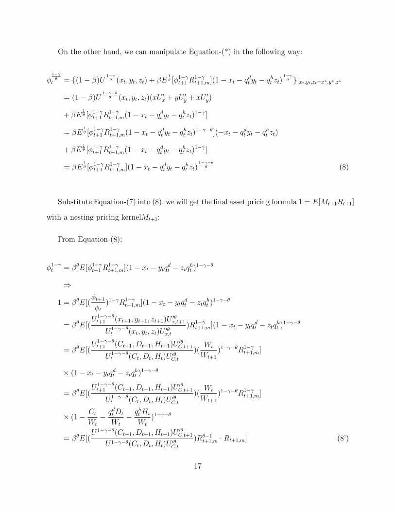
1−γ−θθ (8)

Substitute Equation-(7) into (8), we will get the final asset pricing formula 1 = E[Mt+1Rt+1]

with a nesting pricing kernelMt+1:

From Equation-(8):

φ1−γt = βθE[φ1−γ

t+1R1−γt+1,m](1− xt − ytqdt − ztqht )1−γ−θ

⇒

1 = βθE[(φt+1

φt)1−γR1−γ

t+1,m](1− xt − ytqdt − ztqht )1−γ−θ

= βθE[(U1−γ−θt+1 (xt+1, yt+1, zt+1)U ′θx,t+1

U1−γ−θt (xt, yt, zt)U ′θx,t

)R1−γt+1,m](1− xt − ytqdt − ztqht )1−γ−θ

= βθE[(U1−γ−θt+1 (Ct+1, Dt+1, Ht+1)U ′θC,t+1

U1−γ−θt (Ct, Dt, Ht)U ′θC,t

)(Wt

Wt+1

)1−γ−θR1−γt+1,m]

× (1− xt − ytqdt − ztqht )1−γ−θ

= βθE[(U1−γ−θt+1 (Ct+1, Dt+1, Ht+1)U ′θC,t+1

U1−γ−θt (Ct, Dt, Ht)U ′θC,t

)(Wt

Wt+1

)1−γ−θR1−γt+1,m]

× (1− CtWt

− qdtDt

Wt

− qhtHt

Wt

)1−γ−θ

= βθE[(U1−γ−θ(Ct+1, Dt+1, Ht+1)U ′θC,t+1

U1−γ−θ(Ct, Dt, Ht)U ′θC,t)Rθ−1

t+1,m ·Rt+1,m] (8’)

17

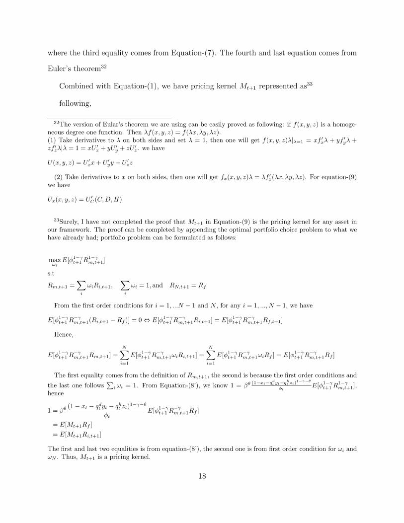
where the third equality comes from Equation-(7). The fourth and last equation comes from

Euler’s theorem32

Combined with Equation-(1), we have pricing kernel Mt+1 represented as33

following,

32The version of Eular’s theorem we are using can be easily proved as following: if f(x, y, z) is a homoge-neous degree one function. Then λf(x, y, z) = f(λx, λy, λz).(1) Take derivatives to λ on both sides and set λ = 1, then one will get f(x, y, z)λ|λ=1 = xf ′xλ + yf ′yλ +zf ′zλ|λ = 1 = xU ′x + yU ′y + zU ′z. we have

U(x, y, z) = U ′xx+ U ′yy + U ′zz

(2) Take derivatives to x on both sides, then one will get fx(x, y, z)λ = λf ′x(λx, λy, λz). For equation-(9)we have

Ux(x, y, z) = U ′C(C,D,H)

33Surely, I have not completed the proof that Mt+1 in Equation-(9) is the pricing kernel for any asset inour framework. The proof can be completed by appending the optimal portfolio choice problem to what wehave already had; portfolio problem can be formulated as follows:

maxωi

E[φ1−γt+1R1−γm,t+1]

s.t

Rm,t+1 =∑i

ωiRi,t+1,∑i

ωi = 1, and RN,t+1 = Rf

From the first order conditions for i = 1, ...N − 1 and N , for any i = 1, ..., N − 1, we have

E[φ1−γt+1R−γm,t+1(Ri,t+1 −Rf )] = 0⇔ E[φ1−γt+1R

−γm,t+1Ri,t+1] = E[φ1−γt+1R

−γm,t+1Rf,t+1]

Hence,

E[φ1−γt+1R−γm,t+1Rm,t+1] =

N∑i=1

E[φ1−γt+1R−γm,t+1ωiRi,t+1] =

N∑i=1

E[φ1−γt+1R−γm,t+1ωiRf ] = E[φ1−γt+1R

−γm,t+1Rf ]

The first equality comes from the definition of Rm,t+1, the second is because the first order conditions and

the last one follows∑i ωi = 1. From Equation-(8’), we know 1 = βθ

(1−xt−qdt yt−qht zt)

1−γ−θ

φtE[φ1−γt+1R

1−γm,t+1],

hence

1 = βθ(1− xt − qdt yt − qht zt)1−γ−θ

φtE[φ1−γt+1R

−γm,t+1Rf ]

= E[Mt+1Rf ]

= E[Mt+1Ri,t+1]

The first and last two equalities is from equation-(8’), the second one is from first order condition for ωi andωN . Thus, Mt+1 is a pricing kernel.

18

Mt+1 = βθ(At+1

At)1−γ−θρ(

Bt+1

Bt

)θ(ρ−α)(Ct+1

Ct)θ(α−1)Rθ−1

m,t+1 (9)

where

At ≡ [Cα + aDα]ρα + bHρ

1ρ and B ≡ [Cα + aDα]

1α

Kernel – 8’ or 9 combine the preference in Epstein and Zin (1989) with more general

composition risks. As one set a = 0 and b = 0, utility function then become U(Ct, Dt, Ht) =

Ct, then from Equation-8’, we can have:

Mt+1 = βθRmθ−1(

Ct+1

Ct)1−γ−αθ(

Ct+1

Ct)(α−1)θ

= βθRθ−1m (

Ct+1

Ct)1−γ−θ

= βθRθ−1m (

Ct+1

Ct)−

θψ (10)

Under different specification of A, B, my specification can degenerate into CRRA and original

setup of E-Z preference. Here, through more general aggregator, composition of C, D and

H will play a role in asset pricing. namely composition risk. For example, from Equation-

(10), we can tell that when θ = 1, EIS ψ becomes ψ = θθ+γ−1

|θ=1 = 1γ, general formula

degenerates into CRRA specification. This observation is confirm as pricing kernel now

becomes Mt+1 = β(Ct+1

Ct)−

1ψ = β(Ct+1

Ct)−γ. Compared to CRRA case, we need a restriction

to take the advantage of E-Z preference: θ > 1, in this case 1− θ − γ < −γ. Pricing kernel

is thus more volatile and more correlated with risky return (Rm part) than CRRA case.

Further more, when γ > 1, θ > 1 is equivalent to γ > θ+γ−1θ≡ 1

ψ. As stated in previous

section, E-Z can improve models’ explanation power against equity premium, when people

prefer early resolution.

19

1.4 Estimate the RRA with Aggregate Data

To study the equity premium, I focus on two versions of asset pricing Euler equations. One

from a simplified version of the general framework, and I will use this simple version to

illustrate the implications out of covariance of aggregate consumption and returns. The

other one follows Equation – (8’) or (9), I adopt this one as granting the model enough

freedom to fit the data. In this general pricing kernel, I calibrate the parameter a and b

to match the expenditure shares of nondurable goods and other expenditure except house

services. The empirical results out of these two specifications are summarized in Table-1.2.

Under the setup in the previous section, I am testing the following Euler equations34:

(EZ) 0 = E[βθ(At+1

At)1−ρ−θρ(

Bt+1

Bt

)θ(ρ−α)(Ct+1

Ct)θ(α−1)Rθ−1

m,t+1(Rt −Rf )] ,

(CRRA) 0 = E[β(Ct+1

Ct)−γ(Rt −Rf )] .

where CRRA case comes from specifying U(c) = C1−γ

1−γ or γ = 1ψ

, pricing kernel follows

Equation-follows Equation-(8’), without resort to Epstein-Zin or other non-traditional pref-

erence parameterization. EZ case follows Equation-(9), with At ≡ [Cα + aDα]ρα + bHρ

1ρ

and B ≡ [Cα + aDα]1α .

If only the excess return equation is to be used in estimation35, I can write the estimation

process of CRRA case into a more explicitly form by approximate the formula by a Taylor

expansion36:

E[R−Rf ] ≈ γCov(gc, R−Rf ) (10)

34For the intuition; one can focus on CRRA case. In general case, the only extra risk is from the compo-sition. For example, the ratio between different kinds of consumption.

35GMM with one moment delivers a similar value of γ36Alternatively, one can explore property of lognormal distribution: if ln(x) ∼ N(µ, σ), then E[x] =

exp(µ+ σ2

2 ). Here, I just use Taylor expansion and the fact that gc and R−Rf are relatively small numbers.

20

where gc ≡ ln(Ct+1) − ln(Ct) and R − Rf is the excess return of equity. Hence, we can

estimate γ well from raw data or Ct and Rt − Rf,t, without resorting to any regression

method:

γ =E[R−Rf ]

Cov(gc, R−Rf )

Where E[.] and Cov(., .) can be estimated as sample average and covariance under the ergodic

assumption. One can tell explicitly that covariance between (relevant) consumption growth

with excess rate is the critical term for equity premium puzzle: since E[R−Rf ] u 6% during

our sample (1961-2016). And covariance between two sequences is determined by correlation

coefficient and individual variance. One can tell from this formula that under CRRA case, the

equity premium implies unreasonably RRA when covariance between the excess return and

consumption growth is low. For example, if we use annual NIPA consumption process, we will

get an estimator around 100, as summarized in Table-1.2. Throughout my whole estimation

process, I follow Campbell (1999) and use the beginning-of-period timing convention as it

gives aggregate consumption data the best chance to fits stock returns.

Since consumption data from NIPA has been filtered and interpolated, the variance of

these sequences got dampened. From the first two rows of Table-1.2, one can tell the corre-

lation between NIPA consumption sequences with the excess return is not low. High implied

RRA is a result of low individual variance and thus low covariance between consumption and

excess return. Hence, Savov (2011) use the garbage data to approximate true consumption

Equation-10 can be proved as following:

0 = E[G−γc (Rt −Rf )]

⇒ E[exp(−γgc))]E[R−Rf ] = −Cov(exp(−γgc), R−Rf )

⇒ (1− γgc +O(1))E[R−Rf ] = −Cov(1− γgc +O(1), R−Rf )

⇒ (E[R−Rf ]− γgcE[R−Rf ] +O(1)) = −Cov(−γgc +O(1), R−Rf )

⇒ E[R−Rf ] ≈ Cov(γgc, R−Rf )

21

process. However, garbage disposable is not a consumption index at all. Moreover, garbage

is measured by weight. Garbage resulting from nondurable goods, like grocery, receives much

less weight than durable goods, e.g., an abandoned running machine.

As an alternative to measuring consumption, I use a more precise index to approximate

aggregate consumption: annual total retail sales (1992-2016). I can get a close estimator

around 25 out of this retail data, while Savov (2011) has 17. Under CRRA specification,

I also try branches of other sequences to represent (approximate) consumption process, for

example, dividend process, auto, Jewelry and watch expenditure from NIPA. As one can

tell from Table-1.2, durable expenditure from NIPA performs relatively better to fit stock

returns, because of higher volatility. To avoid this durability issue, in later sections I exclude

luxury brands focusing on durable goods and try to back out consumption from income and

wealth data of the rich. For example, Richemont is the second largest37 luxury group, I

will not consider its sale when I create my quality goods index since this group focuses on

durables like watches, e.g., IWC Schaffhausen, and writing materials, such like Montblanc.

Beside filtering issuance, all consumption data are time aggregated, and there is a poten-

tial time-aggregation bias: As shown by Breeden, Gibbons and Litzenberger (1989), using

time-aggregate consumption can bias the estimated covariance downward by a factor 0.5.

Hence, given an estimate of RRA, an optimistic adjustment can simply divide it by 2. As

summarized in Table-1.2, the lowest estimator of RRA when we use NIPA consumption data

would be 50, still significantly larger than the upbound 10 in Mehra and Prescott (1985).

And it is worth pointing out that aggregation bias is one reason why calibration results differ

with estimation results.

Furthermore, I include estimator under the EZ-specification in the last row of Table-1.2

with a and b matching the expenditure shares. As one can tell from the table, the estimate

of RRA is 29, which is much less than Hansen and Singleton (1983)38. If one would like to

37LVMH is the largest one and stays in our sample.38I compare my results with Hansen and Singleton (1983), since they use similar estimation process, GMM.

22

consider more portfolios as extra moments, for example, Fama’s SMB and HML factors, one

will get a risk aversion parameter with value 55, significantly lower then Yogo (2006). And

if one is more ambitious to fits Fama-French’s 25 portfolios, I will get a risk aversion with

value 58, as a benchmark Yogo (2006) gets 191. However, House alone, will not generate

a low risk aversion estimator, for example, Davis and Martin (2005)39. Without additional

help, it seems impossible to address equity premium puzzle.

Table 1.2: Risk Aversion Implied by Aggregate Data

Relevant Consumption Series Period Risk Aversion RRA-adjusted Correlation(s.t.d) (s.t.d)

PCE(Total) 1930-2016 85.6 42.8 0.0872(90.2) (45.1)

PCE(Non-durable) 1930-2016 95.54 47.77 0.0836(97.7) (48.85)

PCE(Durable) 1930-2016 51.57 25.78 0.0629(58.1) (29.1)

PCE(Durable:Jewelry and Watches) 1961-2016 -114.26 -57.13 -0.053(122.1) (61.05)

PCE(Durable:auto) 1961-2016 36.84 18.42 0.121(42.1) (21.05)

Retail sale(Grocery Stores) 1992(Jan)-2016(Dec) 24.98 12.48 0.11(31.5) (15.75)

Dividend(S&P 500) 1930-2016 101.96 50.98 0.0333(109.8) (54.9)

Real GDP 1930-2016 55.3 27.65 0.15(61.7) (30.85)

Durable, Nondurable consumption 1930-2016 29.2 14.6 n.aand service flow from House b (35.1) (17.55)

a The table reports the implied RRA for consumption growth using aggregate (approximated) consumptiondata. These results are estimators out of GMM with one moment condition of excess return under differentpreference specification, all rows except the last one are testing E[G−γc (R−Rf )] = 0. Two step of optimalweighting matrix algorithm and Newey and West(1987) adjustment with 5 Lags were adopted throughall estimation processes.

b All other specification are under CRRA. Here we adopt a general pricing kernel Mt+1 =

βθ(At+1

At)1−ρ−θρ(

Bt+1

Bt)θ(ρ−α)(

Ct+1

Ct)θ(α−1)Rθ−1

m,t+1, with At ≡ [Cα + aDα]ρα + bHρ

1ρ and B ≡

[Cα + aDα]1α

1.5 Motivation Evidence: Limited Participation in the

Stock Market

Mankiw and Zeldes (1990) investigates 1984 Panel Study of Income Dynamics(PSID) survey

39Piazzesi, Schneider and Tuzel (2006) adopt a calibration with a tuned process, it is a quantitative success.

23

data and concludes that at most one-fourth American invest in stock market40. However,

one may doubt that one year sample may not suffice to establish that most of the people

are not in the stock market. I thus extend Mankiw and Zeldes (1990) and adopt PSID

in year 1984, 1989, 1994, 1999-2015 (Bi-yearly Survey since 1999)41. PSID is available on

an annual basis from 1968 to 1997, and on a biannual basis since then, but starts to offer

data on equity wealth since 1984. During 1984-1999, PSID only offers equity wealth data in

1984, 1989 and 1994. I summarize the sample in Table-1.3. As one can tell from the table,

Mankiw and Zeldes (1990) gives an optimistic estimator of investor fraction, averagely there

are 18% American have an investment in equity market directly and indirectly. The fraction

of American investing in the stock market has a declining trend, and this is not a problem

with PSID sample.

One can tell the dividend and stock fractions occupied by rich starts to increase since

the mid-1980s. According to Table-1.3, in 2015 only 11.17% of the American families has

positive equity! If one is willing to investigate the fraction of American investing in the stock

market with at least $1000, this number will be much lower than the numbers in the last

column of Table-1.3, for example, Table-1.6 in Appendix.

However, the pattern I find from PSID seems to disagree the recent popularity of mutual

fund. More and more people are entering this market. To address this doubt, I explore a

longer and more comprehensive dataset.

I explore a more comprehensive micro-survey dataset – IRS dataset (administrative tax

records). Though, there is a large gap among national accounts42, the survey, and tax data.

For example, when we investigate PSID, we may conclude that there is one-fourth American

40According to my calculation, there are 17.7% out of the whole sample have positive stock holding, asTable-1.3 shows. Here, positive stock holding is a mild restriction; a family has stock of the value of $1 willbe counted as a shareholder under our conservative assumption.

41I use variable “Equity in stock” (includes shares of stock in publicly held corporations, mutual funds,and investment trusts), variable Index of PSID: S110, S210, S310, S410, S510, S610, S710, S810, ER46952,ER52356, ER58169, ER65366

42For example, national income, such as Census bureau estimates

24

Table 1.3: Sample Observation of Shareholder, PSID:1984-2015

Year Number of Family Number of Family Total number of Fraction of familywithout Investment with positive Investment Family in Survey Staying

in Equitya in Equity in Stock Market

1984 5689 1229 6918 17.77%1989 5614 1500 7114 21.09%1994 6476 2181 8657 25.19%1999 5492 1504 6996 21.50%2001 5729 1677 7406 22.64%2003 6261 1561 7822 19.96%2005 6538 1462 8002 18.28%2007 6809 1477 8289 17.83%2009 7302 1384 8686 15.93%2011 7776 1128 8904 12.67%2013 7970 1090 9060 12.03%2015 8035 1010 9045 11.17%a The table reports the number of family with positive equity, including positive shares of

stock in publicly held corporations, mutual funds, and investment trusts.

hold stock, but this one-fourth may not reflect the true ranking. Fortunately, Piketty, Saez

and Zucman (2016) provide a dataset which combines tax43, survey, and national accounts

data. Piketty, Saez and Zucman (2016) use tax data, which is critical to capture the top

part of income and wealth distribution, and supplement it with survey data to capture the

income not captured in tax data, for example, fringe benefits and tax-exempt transfers to

match national income accounts. It is more comprehensive dataset than PSID.

For this dataset, I plot out the fraction of equity and dividend flow owned by Top 10%

wealthy, in Figure-1.1. In Figure-1.1, equities held through pension plans are counted as

equity holding too44. I thus view this estimate as a conservative one. During 1913-2015,

averagely, 88.1% (89.1%) of equity (dividend) is held by top 10% wealthy. The wealthy are

thus a group who own, operate and manage the firms; they bear most of the risk of the stock

market. This pattern echoes the finding documented in Table-1.6: Only the risk invest a

significant amount in the stock market.

However, there exist no dataset documenting the consumption of rich, I will try several

43Raw data is available after 1962 from annual public-use micro-files created by the Statistics of Incomedivision of the IRS. Piketty, Saez and Zucman (2016) supplement this dataset with the internal use Statisticsof Income (SOI) Individual Tax Return Sample files after 1979. 1916-1962, Statistics of Income, U.S TreasuryDepartment, Internal Revenue Service(Piketty and Saez (2003))

44Data Appendix, Piketty, Saez and Zucman (2016), Page 25.

25

Figure 1.1: Equity held by Top 10% wealthy, annual data, source:Piketty, Saez and Zucman (2016)

ways to “back out” or approximate the consumption of the rich and use the “backed” or

approximated consumption to estimate RRA. In next section, I lay out a simple exercise to

illustrate this idea.

1.6 A Quantitative Exercise

As illustrated in previous sections, aggregate data cannot explain equity return well. One

reason is that of filtering and interpolation issue. However, as a more appropriate index was

adopted, e.g., with retail data I estimate RRA to be around 25, the fifth row of Table-1.2.

In another word, one is still unable to explain the equity return even with an aggregate

consumption approximate without filtering issue.

As we have documented in motivation evidence section, not all people are involved in

the stock market. This phenomenon may be a result of high fixed costs of participating

in the stock market45 or relative high subsistence level. Poor are not willing to incur this

cost to invest or incur this risk. Since the risk is too large for them to hold the risky

45In reality, investment in the stock market involves a lower bound investment amount, even ignoring otherfees like transaction fee.

26

asset, especially when income is close to the subsistence level. Or both of these two factors

contributes, for example when non-rich households have relatively low income compared to

their subsistence46:

U(c) =

(c−x)1−γ

1−γ if c > x

−∞ if otherwise

A mile volatile, risky return means a damaging event to the family, as c → x, where x is

subsistence level, marginal Utility will become infinity. Put in another way, current equity

premium is not high enough to attract poor. Hence, the stock market is mainly occupied

by the wealthy and rich. Limited participation thus predicts a low covariance between the

aggregate consumption and stock returns, since an average American does not even bear the

risk from the stock market. Aggregate consumption, no matter how we are to measure it, in-

cludes the consumption of all families. Using this aggregate sequence potentially contributes

to the Equity Premium Puzzle since the covariance is down-biased.

As one can tell from Table-1.3 and Figure-1.1, top 10% wealthy is the player in stock

market. I thus make a simplifying assumption to facilitate our exploration exercise: a

representative agent is assumed to have ln utility function. Without any market structure

friction, consumption will be a fix fraction of rich’s wealth. The growth rate of consumption

of rich can be then represented by the growth rate of the wealth of the rich. Then we use

this “backed” consumption process to replicate the exercise of Mehra and Prescott (1985).

This structure “back-out” method can be extended to a general case, using only income

and wealth data without the information on investment portfolios: for any given(guessed)

RRA, one can solve a consumption policy function. Then we “back out” rich’s consumption

data from income and wealth data. Furthermore, this backed out data can be used to

46Under subsistence assumption, the pricing kernel under EZ preference will not be as simple as Equation-(9) and derivation method should change accordingly, since value function is not homogeneous of degree oneanymore.

27

Figure 1.2: Implied Risk aversion Coefficient by backed-consumption of rich

calibrate RRA again, as Mehra and Prescott (1985) does. And the true estimator should

be the one at which guessed value agrees with the calibrated one. I will leave general case

exploration for later sections. Here we merely explore the backed-consumption process of

top income under log preference specification.

The exercise of Mehra and Prescott (1985) can be implemented as following: calibrate

the income process by a two-state Markovian process, matching the expected, variance and

first-order auto-correlation of income growth. And under CRRA framework, earning/price

ratio(policy function) will thus be a function of the only state variable(income growth).

Expected risky return can thus be calculated. I used policy function iteration algorithm as

stated in the Numerical appendix.

Given a backed-out consumption process, we take it to be the “true” consumption process

and parameters except time discounting rate and RRA are calibrated to match its sample

28

average, variance and first-order autocorrelation. The time discounting rate is fixed at 0.98,

then implied excess return is plotted against varying RRA, as in Figure-1.2. To justify a

6% equity premium, rich people in top 10% quantile will need an RRA around 10, rich

people in top 5% quantile will need an RRA around 7. The mechanism here is that top

incomes are more volatile than aggregate income (GDP). The relatively high volatility of

rich’s “consumption” can be justified by risk-sharing mechanism: workers get a fixed salary,

and share-holder afford whatever the firm earns or losses. Furthermore, rich’s income is

more persistent than GDP, echoing the mechanism in Bansal and Yaron (2004). It is worth

pointing out that the persistent should not be too large. As well-illustrated in Boldrin,

Christiano and Fisher (1997), too persistent consumption process will deliver a wired pattern:

when RRA increases the implied excess return decreases. If I use the backed consumption

process to estimate RRA, estimate are 11.34 for Top 10%, 10.8 for Top 5%, 9.67 for Top 1%.

In next two sections, I start to design and create a consumption index to approximate

rich’s consumption. The data we use in previous and later sections will also be documented

in next section.

1.7 Data

To have an index to measure quality goods, we construct sale data of Tiffany, Sakes, Gucci47,

Neiman Marcus, LVMH, Hermes, Burberry, Bulgari48, Gucci49 and Kering50. Many groups

here own branches of brands. For example, LVHM owns 56 brands, not only Louis Vuitton,

but LVMH also owns Loro Piana, Kenzo, Givenchy, and Berluti. Bering51 maybe not as

47Now Belongs to Bering, collected sales in U.S area from Annual Reports48independent until 2011, now belongs to LVMH, collected sales in U.S area from Annual Reports49independent until 2004, belongs to Kering now50There is another famous luxury group, Richemont, which mainly focuses on jewellery, watches, leather

products, and writing instruments. But as we discussed in the early sections, we try our best to focus onthe luxury brands not concentrate on durables.

51Formerly named Pinault-Printemps-Redoute

29

famous as LVMH. It transforms into a luxury retailer after 2004. However, it owns well-

known luxury brands like Brioni, YSL. All sales data are restricted to turnover in U.S area

and taken from their original annual reports.

Since most brands have products like leather products and clothes, durability is a po-

tential issue, though BEA includes them in non-durable goods. A baby cashmere52 sweater

by Loro Piana or a handbag by Hermes may last for over ten years. However, this is one

character of quality goods. Not only they provide tremendous consumption experience, such

like texture and fitting, but also they can offer them consistently and during a more extended

period.

As a solution to this durability. One can argue that fashion is fickle. Their products are

updated seasonly. However, as we are focusing on the quality part of luxury brands, fashion

is not our concern. Hence, I instead resort to two other indices and another approach: (1)

Quality Grocery, I estimate the sale of Premium Grocers by aggregate the sales of four

public grocery firms: Whole Foods Market, The Fresh Market, Sprouts Farmers Market,

and Fairway Group Holdings. I choose premium grocers as they focus on providing grocery

with high qualities. (2) Luxury lodging service. According to ”J.D. Power 2015 North

America Hotel Guest Satisfaction Index”. I selected out the most luxury hotels listed53.

I then deleted those who has minor or even no operation in U.S, for example Gran Melia

hotel. They focus their business in Spain. Fortunately, most of these hotels belong to several

hotel groups: Marriott(formly name Hot Shoppes,then Marriott Hotel corporation), Hilton,

52Gathered only from the under fleece of Hyrcus goat kids, Baby Cashmere is exceptionally fine, at just13 microns. It takes the fleeces of 19 child goats to make a single sweater.

53Listed hotels: Bulgari Hotels and Resorts (Marriott Hotel Development), Park Hyatt, Mandarin Orien-tal Hotel Group(a member of the Jardine Matheson Group), St. Regis Hotels & Resorts(Starwood HotelsSystem), Ritz-Carlton Hotel Company(belongs to Marriott International), Waldorf Astoria Hotels & Re-sorts(Owned by Hilton Worldwide), Four Seasons Hotels,The Peninsula Hotels, Luxury Collection(Marriott),Sofitel :French luxury hotel chain brand under AccorHotels, Rosewood Hotels & Resorts, Conrade Hotels(Hilton Group), JW Marriott(Marriott Group), Andaz (Hyatt), W Hotel (S.P.G Marriot), Renaissance Ho-tels (Marriot), Autograph Collection Hotels (Marriot), Edition (Marriot), Curio(Hilton), Westin(StarwoodHotels and Resorts Worldwide Or Marriot), Le Meridien (SPG), InterContinental (InterContinental HotelsGroup), Marriott, Hilton Hotels & Resorts, Hyatt Gegency (Hyatt), Sheraton(Starwood Hotels and ResortsWorldwide), Crowne Plaza(InterContinental Hotels Group)

30

SPG(now belongs to Marriott), InterContinental Hotel Groups and Hyatt. I obtain their

sales in U.S from their annual report. Hilton(1967-2005,2013-2015), Marriott(1968-2015)

and InterContinental Hotel Groups(2003-2015).

For the other approach, I explore the data on income, wealth and investment portfolio

of the rich to estimate their consumption. Data on after-tax real income per capita, labor

income share, real wealth, investment portfolios, equity wealth distribution and dividends

distribution is from data appendix II of Piketty, Saez and Zucman (2016)54 . Return data

of relevant categorized assets is from data appendix I of the same paper.

For returns, the stock return is measured as the return on the value-weighted NYSE-

AMEX portfolio from the Center for Research in Security Prices (CRSP). I follow Fama

and French (1993) to define excess return as stock return minus one-month Treasury bill

rate. Along with three FamaFrench factors, return data and one-month Treasury bill rate

are available from French’s Website55. The three FamaFrench factors are excess returns on

the market portfolio, returns on the SMB portfolio(small minus big), and returns on the

HML portfolio(high(book-to-market) minus low). The excess market return is the return on

a value-weighted portfolio of NYSE, AMEX, and Nasdaq stocks minus the one-month T-bill

rate. The SMB and HML portfolios are based on the six FamaFrench benchmark portfolios

sorted by size (breakpoint at the median) and book-to-market equity (breakpoints at the 30th

and 70th percentiles). The SMB return is the difference in average returns between three

small and three big stock portfolios. The HML return is the difference in average returns

between two high and two low book-to-market portfolios. The 25 FamaFrench portfolios are

constructed from an independent sort of all NYSE, AMEX, and Nasdaq stocks into quintiles

based on size (i.e., market equity) and book-to-market equity. Data on the FamaFrench

factors and portfolios are again obtained from Kenneth Frenchs web page.

54Available through http://gabriel-zucman.eu/usdina/55http://mba.tuck.dartmouth.edu/pages/faculty/ken.french/data library.html

31

Figure 1.3: Synthetic Consumption of the Rich and Excess Return, 1945-2012, Annual Data

1.7.1 Synthetic Consumption by the Rich, Backed from Wealth

and Income Data

In this section, I explore the dataset provided by Piketty, Saez and Zucman (2016) to estimate

the consumption by the rich. In the following sections, I will explore data from public firms

to create another three indices to approximate the consumption by rich.

From data Appendix II of Piketty, Saez and Zucman (2016), I get data on income, labor

share, investment portfolio, and per capita wealth data of the Top 10%, 5% and 1% wealthy.

I make an empirical conjecture that the wealthy people are the same as people with highest

after-tax income. Since this assumption holds just approximately, I view my estimate of

consumption of the rich as an approximate. And since this conjuncture may not hold for

the top 1%, in the main text, I only report the estimates of 10% and 5%.

One can view my process as an inverse procedure in Saez and Zucman (2016). Section VI

of Saez and Zucman (2016) tries to estimate the saving rate of rich. Here, I try to estimate

the synthetic consumption of rich.

32

Furthermore, I back out consumption by the following formula:

Wt+1 = Rm,t+1 · [Wt + Yt − Ct]

where Yt and Ct denote the labor income and consumption during period t, and Wt represents

the wealth the end of period t. Rm,t+1 is the real return of wealth. Here I use the assumption

that labor income comes before capital income. Alternatively, in appendix I used Wt+1 =

Rm,t+1 · [Wt − Ct] + Yt to replicate the whole estimate process here. Our results are robust

to this modification.

Since I need data from Wt and Wt+1 to estimate Ct, hence the estimated Consumption

ranges from 1927-2012. And to estimate the wealth return of the rich, I also make an

approximation assumption: people obtain the same return of the same kinds of assets.

To estimate the real return of wealth, I append my data with the average real return of

various kinds of asset: Home, Equity, Fixed income asset, Pension, and Business. Return

data comes from data Appendix Table-I56. To estimate the wealth return of the rich, I also

make an approximation assumption: people obtain the same return of the same kinds of

assets because of data restriction.

Following the formula, I estimate the consumption by top 10% and 5%. The growth rate

of these consumption process is plotted against excess return from 1927-2012 in Figure-1.3.

One can tell that these sequences comove with excess return closely.

The GMM RRA estimate out of a single moment (1927-2012) are 4.88 and 3.23 for the

top 10% and 5%. For period 1960–2012, the RRA are 3.011 and 2.941.

To show the low estimate of RRA is not a result of this approach, I next focus on sales

data to create three indices to approximate the consumption by the rich in following sections.

56Available through http://gabriel-zucman.eu/usdina/ or https://sites.wustl.edu/xiwang/research/.

33

Figure 1.4: Luxury sales and Excess Return, 1962-2015, Annual Data

1.7.2 Quality Goods and Equity Premium

In this section, I start to use my constructed indices to approximate the rich’s consumption

and estimate RRA. One uses the sales of luxury brands in the U.S. Another one adopts

quality grocery to price the asset. Another uses luxury lodging service. As a robustness check,

I estimate and use the stock of quality goods, instead of sales to approximate consumption

flow. The estimators we get are summarized in Table-1.4. As one can tell at first glance, all

these estimates are below ten after adjustment even though we are using annual series.

Sales of Quality Goods

I plot the growth rate of constructed quality goods index against excess return in Figure-1.4.

Since the goods sold by each group are close substitutes, we merely sum them up to get an

aggregate index. As one can tell from Figure-1.4, there is a positive co-movement over time

between excess stock returns and sales growth for quality goods. And this co-movement

becomes more significant when it enters the late-1980s, when we include more and more

brands in our quality goods index, before late-1980s, Tiffany is the only one in our sample.

34

Figure 1.5: Premium Grocery sales and Excess Return

The overall correlation(covariance) between quality sales and excess return is 0.285(0.731),

while the correlation is 0.208(0.409) during 1961-1989. Furthermore, our index is much more

correlated with rich’s income(Top 10%) than NIPA nondurable consumption index: 0.368

against 0.113 during 1961-2014, while the correlation between aggregate consumption and

income is 0.301 during the same period. Our index thus offers a good approximate to rich’s

consumption.

With sale index of quality goods, we estimate RRA by GMM with one moment condition

under CRRA specification, hence we restrict our ability to fit the data. Estimate of RRA

out of this process is 9.48, without any adjustment. This estimate of risk aversion is an

order of magnitude less than estimator by using (non)durable process, which is above 50 as

summarized in Table-1.2.

However, there are still two issues about our constructed index:(1) Durability. Quality

goods, by definition, lives longer than there peer product. (2) Before the late-1980s, Tiffany is

the sole company in our sample. In next subsections, we tend to adopt another two datasets

to attack these two problems and confirm that our estimator is robust if one investigates a

nondurable and longer quality consumption data.

35

Premium Groceries

Since the quality goods, I list in the previous section includes clothes, Jewelry, and handbags,

durability is an issue. The ideal index should be nondurable goods or service. I adopt and

construct two indexes to approximate them. Focus here is the same with previous sections:

quality goods, for example, organic fruits, olive oil and luxury lodging service like Ritz-

Carlton.

As an approximate quality nondurable goods and comparable series to the retail data

we adopt in the previous section, we adopt annual(quarterly) sale of Premium Grocers. I

estimate the sale of Premium Grocers by aggregate the sales of four public grocery firms5758:

Whole Foods Market, The Fresh Market, Sprouts Farmers Market, and Fairway Group

Holdings. I choose premium grocers as they focus on providing grocery with high qualities.

For example, Whole Foods Market is the first certified organic grocer in U.S, which means

it ensures, to National Organic Program standards, organic integrity of the heterogeneous

products from the time they reach stores until they are placed in a shopping cart. Even

though organic foods do not have a higher content of nutrients, studies have found they have

a lower level of anti-nutrients, cadmium and pesticide residues. The sales and excess return

are plotted in Fig-1.5. Estimate of RRA with GMM(one moment) is 17.47, without any

adjustment. Since whole food has the longest historical data, we adjust our return according

to its fiscal year, which ends in September. The estimator of RRA by using whole food alone

is 19.38.

57There are several large premium groceries stay private, for example, Trader Joe’s and HEBs CentralMarket.

58Though Safeway, Kroger, and even Walmart have expanded their premium and organic offerings inrecent years. They used not to focus on premium grocery market.

36

Figure 1.6: Luxury Lodging and Excess Return

Luxury Lodging

In my main index, Tiffany is the only sample we have before the late-1980s. And as we can

tell from Table-1.2, Jewelry did a not bad job to explain stock return. One may doubt the

explanation power to some degree, at least before the 1980s, may come from this durability.

To address this issue, we adopt luxury lodging service to approximate consumption flow.

From ”J.D. Power 2015 North America Hotel Guest Satisfaction Index”. I then further

restrict our sample to those hotel brands focusing in U.S. For example, Bulgari Hotels, and

Resorts, Park Hyatt, St. Regis (Starwood Hotels System), Ritz-Carlton Company(Marriott),

Waldorf Astoria Hotels & Resorts(Owned by Hilton Worldwide). Most of these hotels belong

to four hotel group: Marriott (formerly name Hot Shoppes, then Marriott Hotel corporation),

Hilton, Four Season(not Public), Hyatt. Hence, we collect sales of full-service and luxury

sales from their annual report and construct a luxury lodging service index. The sales and

excess return are plotted in Fig-1.6. Since there is a potential reservation lag, people use

to book a room in advance; they plan this consumption in advance. I thus take a one-year

lag to implement estimation process. Estimate of RRA with GMM(one moment) is 15.05,

37

Figure 1.7: Index of Stock of Quality Goods and Excess Return

without any adjustment.

Robust check: Add in Depreciation

By adopting different sources of data, we tried to address durability issue in previous sub-

sections. In this subsection, we provide further evidence that durability is not the reason

driving our results. Parker and Julliard (2005) argue that the stock of durables should be

cointegrated with durables expenditure. In other words, in long-run durable expenditure

can represent the stock of durables. No adjustment is necessary, as long as we use a growth

rate of a longer horizon, e.g., three years. Besides this long-horizon growth rate, we estimate

the stock of durable by assuming a depreciation rate.

By using the quality goods index we have constructed, we back-out the stock of quality

goods,St, from the flow, Ft by assume a depreciation rate59:

St = St−1(1− δ) + Ft

59If δ = 1, then quality goods are perishable goods, and sales date can represent consumption flow.

38

Where δ is the rate at which the durable good depreciates. Then 1/δ is the expected lifetime

of durable. By setting expected durability to be 1.25, 2 and 2.5 years, we can back out

a sequence of stock. The RRA Estimates out of this sequence are 14.01, 17.40 and 19.9

without any adjustment. And these stocks data are plotted against excess return in Fig-1.7.

I summarize our empirical finding by using quality goods sequences in Table-1.4. I lay out

several summary tables with more moments conditions: Fama-French’s three factors and 25

portfolios. In brief, we have a much smaller estimator of RRA when comparing with previous

literature.

Furthermore, as another kind of robustness check, we implement estimation with more

moment conditions and explore the cross-sectional average return in next sections.

Table 1.4: Risk Aversion Implied by quality goods and service data

Relevant Consumption Series Period Risk Aversion RRA-adjusted Correlation(s.t.d) (s.t.d) with excess return

Consumption by Top 10% 1927-2012 4.88 2.06 0.367(4.11) (2.06)

Consumption by Top 5% 1927-2012 3.23 1.62 0.243(2.97) (1.49)

Quality Goods(Total) 1961-2016 9.48 4.74 0.285(12.2) (6.1)

Quality Goods(1.25 Years) 1971-2016 14.01 7.01 0.164(16.7) (8.35)

Quality Goods(2 Years) 1971-2016 17.40 8.70 0.1524(22.1) (11.1)

Quality Goods(2.5 Years) 1971-2016 19.90 9.95 0.1417(25.3) (12.65)

Premium Grocery 1993-2016 12.91 8.735 0.1207(15.1) (9.55)

Quality Lodging 1969-2016 15.05 7.53 0.246(19.7) (9.85)

a The table reports the implied RRA for consumption growth using quality goods consumptiondata. These results are estimators out of GMM with one moment condition of excess returnunder different preference specification, all rows are testing E[G−γc (R − Rf )] = 0. Two stepof optimal weighting matrix algorithm and Newey and West(1987) adjustment with 5 Lagswere adopted through all estimation processes.

39

Figure 1.8: CCAPM can explain almost nothing cross-sectionally

Figure 1.9: 1927-2012, Realized versus predicted excess returns(25 Portfolio), Top Consumption

40

1.8 More Moment Conditions

In previous sections, the estimation burden we imposed on our CRRA model is mild: only

one asset pricing moment, requiring our model to fit equity premium data. However, an

asset pricing Euler equation is more than a moment restriction on market excess return.

For example, there are Euler equations restricting the moment condition of risk-free rate,

three Fama French factors and more extremely 25 or 100 portfolios formed on Size and

Book-to-Market, as defined in Fama and French (1993).

I thus adopt two-step procedure of GMM method with Newey and West(1987) adjust-

ment(5 Lags60). To better assess the performance of our constructed indexes, we mainly

lay out another three strings of estimation. In one string, we impose four moment condi-

tions: Euler equations of Market excess return, risk-free rate(one-month T-bill rate), SMB

and HML excess return. The last two are as defined in Fama and French (1993), for com-

pleteness of our article, we rephrase the definition as follows: SMB (Small Minus Big) is

the average return on the three small portfolios minus the average return on the three big

portfolios. HML (High Minus Low) is the average return on the two value portfolios minus

the average return on the two growth portfolios. One can view them as two different returns

of two pairs of portfolios.

Another two strings impose 27 moments condition: Euler equations of Market excess

return, risk-free rate(one-month T-bill rate) and pricing formula for 25 portfolios formed on

Size and Book-to-Market(Value and Equally weighted), definitions and summary statistics

are reserved in Appendix.

Furthermore, all these estimation processes include three parts:(1) unconditional moment

estimation (2) Conditional moment estimation with lag consumption growth as instruments

(3) Conditional moment estimation with lag consumption growth and risk-free rate as in-

struments. I adopt our two quality index: quality goods index and luxury lodging index. As

60Our results are robust if one would like to adjust more lags.

41

a benchmark, we adopt nondurable consumption and service and total consumption as the

benchmark.

Estimation results are summarized in Table-1.7, 1.8 and 1.9. As one can tell from these

tables, adding more moments does not increase our estimation of RRA if we use our quality

index, but standard deviation got reduced. For example, the first row of Table-1.8, the

lowest RRA estimate is 2.17 with s.t.d 0.80, within the range pointed out in Mehra and

Prescott (1985). However, when we adopt aggregate consumption index, equity premium

persists. For example, the last row of Table-1.8, RRA is estimated to be 61.6 with s.t.d

12.34, significantly higher than 10.

1.9 Cross-Sectional Expected Return

In this section, we evaluate the ability of quality indices to price the average returns on

different portfolios of stocks besides the excess market return. If our quality indices approxi-

mate the rich’ consumption, stocks that have more exposure to this consumption risk should

have a higher expected return. In this section, we consider the ability of our quality indices

to explain the cross-sectional difference of expected return across portfolios.

I am considering 25/100 portfolios formed on Size and Book-to-Market as test portfo-

lios. As a benchmark, we compare our fitting to Fama-French three sector, CCAPM, and

CAPM models. In sum, Fama-French three sector model dominates. Quality indices perform

better(has lower MAE) than the other two models.

Cross section specification emerges from the linearization of pricing kernel. SupposeMt+1 is

a pricing kernel, which is a linear function of some factors, e.g. consumption growth rate in

42

Figure 1.10: 1927-2012, Realized versus predicted excess returns(100 Portfolio), Top Consumption

CCAPM Model.

E[Mt+1(Ri,t+1 −Rf )

]= 0 , for i = 1, 2, . . . , N

Mt+1

E[Mt+1]= −

[α + θTft+1

].

Combine these two equations, we have a cross sectional relationship:

43

Figure 1.11: Realized versus predicted excess returns(25 Portfolio)

E[(Ri,t+1 −Rf )

]= −Cov(Mt+1, Ri,t+1 −Rf )

E[Mt+1], for i = 1, 2, . . . , N

= Cov(θTft+1, Ri,t+1 −Rf ))

≡ θTΣf,i

= θTΣf,f Σ−1f,fΣf,i︸ ︷︷ ︸≡βi

= Factor Risk Premium · βi

Portfolios with higher risk exposure(βi) should enjoy a higher excess return. I visualize

our results in Figure-(1.8) to (1.12). In Figure-1.8, we plot the predicted average return

implied by CCAPM model to actual returns, left panel is the case of 25 portfolios and right

44

Figure 1.12: Realized versus predicted excess returns(100 Portfolio)

for 100 portfolios. You can tell from the figure that CCAPM can almost justify nothing in

the difference between portfolios.

On the other hand, Fama-French model(FF) is (one of) the best among our candidate to

fit cross-sectional returns. From 1960 – 2015, one can tell from upper left panel of Figure-

(1.11) and (1.12), predicted returns almost lines up with actual ones. Moreover, though our

quality indices cannot beat FF, it beats CAPM and CCAPM. For example, MAE of quality

goods index to fit 100 portfolios is 0.026, while MAE of CCAPM and CAPM are both 0.028.

From 1927 – 2012, one can tell from Figure-1.9 and 1.10 that my top consumption is not

dominated by FF method.

45

1.10 Conclusion

In this article, we reviewed the fact that equity premium persists under the model without

the help of tuned process or modified data. I argue that the equity premium puzzle is partly

because we are using a polluted consumption data. I layout two pieces of evidence to show

that the stock market involves only a small fraction of people. They are the top wealthy

people in U.S. As a way to approximate their consumption process, we discuss and create

indices of quality goods and services.

By using several quality indices, we find that marginal utility of the investors(the wealthy)

co-moves significantly with the return on equity. The covariance of quality indices and excess

returns implies a coefficient of relative risk aversion estimate lower than the one estimated by

using aggregate consumption. To avoid the issue of durability issue, we restrict our brands

sampling during the process of creating quality goods index. Moreover, we also provide two

sequences of nondurable and service indices as alternative quality goods and service indices.

In general, our estimators of RRA can be reduced in a reasonable range according to Mehra

and Prescott (1985) and lower than those estimators in existing literature. Furthermore, our

indices provide a better cross-sectional fitting than CCAPM and CAPM.

46

1.11 Appendix

1.11.1 An Empirical Estimation for Habit Formating Framework

It is hard to find a empirical corresponds for habit formation models. All papers based on

Habit formation are using quantitative assumptions to characterize the property of habit

term.

On the other hand, utility with a varying subsistence level can also be viewed as a habit

formation preference with exogenous varying habit. Put in another way, subsistence level

approximates habit term. To approximate this subsistence level, we use poverty thresholds,

which can be understood as the lowest income to stay alive.

This subsection will explore the successful specification being used in previous literature:

Habit difference. In the remaining text, I will explain the data source. Then, a model with

habit formation are laid out and moments conditions are derived, And I summarize the

estimation results out of a two stage GMM with HAC adjustment.

There are two slightly different versions of the federal poverty measure: poverty thresholds

and poverty guidelines.

Poverty thresholds are the first version of poverty measure, being updated by Census

Bureau on yearly base since 1959. It is the number used by the Census Bureau to determine

the poverty status of families. Thus, all official poverty population are calculated by using

this sequence. This data sequence is available from Census Bureau’s website, 1959-2016.

The other index, poverty guidelines, is created by Department of Health and Human

Services(HHS). This index is a simplification of the former one, and used for administrative

purposes, e.g. determining eligibility for certain federal programs. This data sequence is

available from the website of HHS, 1982-2016.

Consumption per capita and inflation data are from BEA’s website.

To estimate the subsistence (habit) term X in Utility function (C−X)1−γ

1−γ , I use Poverty

47

Line (Guide) data, consumption per capita, and H-P filter.

To estimate long-run consumption per capita Ctrendt Tt=1, I use λ = 100 (annual data) to

extract the long run trend from ln(Ct)Tt=1 , then long-run consumption can be backed by

take a exponential transformation of the resulting sequence.

Subsistent level or habit term should be a fraction of this long-run term. To pin down

this fraction, I take the average of the ratio between Poverty line (Guide) and consumption

per capita. The fractions are pined down as 0.461 and 0.376.

Hence X itTt=1 are estimated as:

X it = θi · Ctrend

t

where Ctrendt is the long-run component of consumption per capita in period t. θ1 = 0.461

and θ2 = 0.376.

Thus RRA (γ) estimate is from GMM with the moment:

E[β(Ct+1 −Xt+1

Ct −Xt

)−γ(R−Rf )]

= 0

To show my results are robust to my choice of λ = 100 in HP filter, I document the

results with other value of λ in following table.

1.11.2 Numerical Algorithm: Policy Iteration

In this section, we layout a general version of our numerical algorithm we used in this article

to solve our model. This method can be used to solve Long run risk model or Habit formation

48

Table 1.5: Estimated RRA with Habit formating specification

λ in HP filter RRA1 RRA2

100 35.91 38.75120 36.07 38.77150 36.20 38.79180 36.29 38.84300 36.82 38.98500 37.37 39.1480 35.89 38.7260 35.77 38.7530 35.97 38.92

method too. To fix idea, we lay out several notation first: For any period t, exogenous state

variables are zt, endogenous state variable is st. In general, zt and st can be vectors. In our

case, zt is the growth rate of consumption, st is the stock holding. In Long-run risk setup,

zt will be the volatility and consumption.

Given any realization of exogenous state variables, our goal is to find a optimal choice

variable and endogenous state variable for next period, namely Policy function. Since st

here is restricted to be 1, as required by market clearing condition. I do not really have an

endogenous state variable. Hence, the goal here is to find policy function for consumption

and asset price.

Given any realization of zt and policy functions from last iteration(k), ck(z, F,B), qk(z, F,B):

The equations we are to explore under CRRA setting is:

ct(zt, st+1) = (U ′)−1(EFt [βU ′(ck(zt+1, st+1))Rf ])

qt(zt) = (EFt [βU ′(ck(zt+1))

U ′(ck(zt))(qt(zt+1, st+1) + d(zt+1))] (A.1)

where (U ′)−1 is inverse function of U ′(.) and ck(z, st+1) is policy function from iteration k.

49

EFt denotes an expectation operator conditional on information set at period t. Since our

model is Markovian, Ft is sufficient for agents to form an expectation. Generally, policy

function is defined on state variable space. It is worth pointing out that ct(zt, st+1) and

qt(zt, st+1) is not a policy function yet, since B′ is not a state variable, at least not for period

t. And generally, we can choose zt+1 instead of searching the optimum at period t, following

endogenous grid method.

Under endowment economy setting, numerical problem is dramatically simplified by two

reason: (1) st is set to 1 exogenously, because of asset market clearing condition. Thus

endogenous grid method can be avoided (2) consumption policy function can be avoid, since

all the consumption comes from dividend, which will be assumed exogenously. Hence the

only relevant policy function is Equation-(A.1).

Policy iteration process goes as following:

(1) Specify a initial guess of policy function, which defined on exogenous state space. I

denote it as q0(z);

(2) Given any policy function qk(z) from k-th iteration. the policy function for next

iteration is defined as

For any zt in the support set of state variable, and expectation is formulated by a tran-

sition matrix, which can be generated through Tauchen method or Rouwenhorst method.

qk+1(zt) = E[βMt+1(qk(zt+1) + d(zt+1))|zt]

For example, under E-Z setting Mt+1 = βθ(At+1

At)1−ρ−θρ(Bt+1

Bt)θ(ρ−α)(Ct+1

Ct)θ(α−1)Rθ−1

m,t+1, with

At ≡ [Cα + aDα]ρα + bHρ

1ρ and B ≡ [Cα + aDα]

1α . A, B, C will be all pre-specified

function of exogenous variables. Under CRRA setting Mt+1 = U ′(ck(zt+1))U ′(d(zt))

. And again d(.) is

exogenous specified by our model.

(3) Calculate the distance between the new policy function and the old one. Keep iter-

50

ating until the distance drops below a prior setting, for example 10−6.

This procedure can also be used to solve long-run risk and habit formation model. As

long as within a endowment economy, extension is straightforward.

51

1.11.3 More Statistical Tables

Table 1.6: Sample Observation of Shareholder,PSID:1984-2015

Year Total number of Number of Family Fraction of familyFamily in Survey with more than $1000 staying inside

Investment in Equitya

1984 6918 960 13.88%1989 7114 1267 17.81%1994 8657 1924 22.22%1999 6996 1376 19.67%2001 7406 1481 20.00%2003 7822 1387 17.73%2005 8002 1329 16.61%2007 8289 1360 16.41%2009 8686 1238 14.25%2011 8904 1020 11.46%2013 9060 1005 11.09%2015 9045 937 10.36%a The table reports the number of family with positive equity, includ-

ing positive shares of stock in publicly held corporations, mutualfunds, and investment trusts.

52

Table 1.7: Risk Aversion Estimation with Four Moment Condition

Relevant Consumption Series Period Risk Aversion Instruments Instrumentsabc

with gc,t−1 with rft−1 and gc,t−1

(s.t.d) (s.t.d) (s.t.d)

Quality Index 1961-2016 7.838725 7.765891 7.550789(2.935593) (2.893989) (2.694529)

Luxury lodging 1961-2016 20.18627 17.72594 17.38974(10.60995) (3.631274) (3.138696)

Nondurable goods 1961-2016 39.73827 38.18957 37.41744and Service (27.70305) 16.6783 (13.91141)

Total Consumption 1961-2016 49.82824 47.54617 47.86384(17.86918) (13.36898) (12.40958)

a The table reports the implied RRA for consumption growth using quality goods consumptiondata. These results are estimators out of GMM with four moment condition of excess return underRRA specification. Two step of optimal weighting matrix algorithm and Newey and West(1987)adjustment with 5 Lags were adopted through all estimation processes.

b Four moments includes pricing risk free rate, pricing equity premium, SMB and HML Fama-French 3 factors

c Instruments estimation is essentially estimating conditional moment conditions.

Table 1.8: Risk Aversion Estimation with 25 Size to Book Portfolio(ValueWeight)

Relevant Consumption Series Period Risk Aversion Instruments Instrumentsabc

with gc,t−1 with rft−1 and gc,t−1

(s.t.d) (s.t.d) (s.t.d)

Top 10% Consumption 1961-2016 2.168263 2.740748 2.666241(.8017915) (.6622103) (.2561315)

Top 5% Consumption 1961-2016 1.3628 1.875603 1.942435(.6635609) (.363467 ) (.2496861)

Quality Index 1961-2016 9.312636 7.765891 7.603876(2.53162) (2.893989 ) (2.801075)

Luxury lodging 1961-2016 18.72369 17.72594 17.45517(2.288341) (3.631274) (2.607822)

Nondurable goods 1961-2016 -90.0424 38.18957 38.70487and Service (22.49862) (16.6783) (15.20182)

Total Consumption 1961-2016 61.66475 47.54617 48.04298(12.34485) (13.36898) (12.50159)

a The table reports the implied RRA for consumption growth using quality goods consumptiondata. These results are estimators out of GMM with Twenty seven moment conditions ofexcess return under RRA specification. Two step of optimal weighting matrix algorithm andNewey and West(1987) adjustment with 5 Lags were adopted through all estimation processes.

b Twenty seven moments includes pricing risk free rate, pricing equity premium, and 25 Portfo-lios(Value Weighted) Formed on Size and Book-to-Market.

c Instruments estimation is essentially estimating conditional moment conditions.

53

Table 1.9: Risk Aversion Estimation with 25 Size to Book Portfolio(EquallyWeight)

Relevant Consumption Series Period Risk Aversion Instruments Instrumentsabc

with gc,t−1 with rft−1 and gc,t−1

(s.t.d) (s.t.d) (s.t.d)

Top 10% Consumption 1961-2016 2.340826 2.909688 2.872546(.8048266) (.636315) (.4408074)

Top 5% Consumption 1961-2016 1.444308 1.968068 1.869321(.665057) (.2714227) (.3265898)

Quality Index 1961-2016 11.3465 11.30186 10.9427(2.024994) (0.8420869) (1.093398)

Luxury lodging 1961-2016 18.87187 17.0533 17.25982(2.096608) (1.745999) (1.473657)

Nondurable goods 1961-2016 -53.03731 -37.7818 -35.20731and Service (23.91825) (3.272319) (1.303017)

Total Consumption 1961-2016 61.18114 60.37082 62.31743(11.58245) (6.324507) (4.095732)

a The table reports the implied RRA for consumption growth using quality goods consumptiondata. These results are estimators out of GMM with Twenty seven moment conditions ofexcess return under RRA specification. Two step of optimal weighting matrix algorithm andNewey and West(1987) adjustment with 5 Lags were adopted through all estimation processes.

b Twenty seven moments includes pricing risk free rate, pricing equity premium, and 25 Portfo-lios(Equally Weighted) Formed on Size and Book-to-Market.

c Instruments estimation is essentially estimating conditional moment conditions.

54

Chapter 2

The Quantity Theory of Money: An

Empirical and Quantitative

Reassessment

2.1 Introduction

The Quantity Theory of Money (QTM) has been at the heart of Monetary Economics since

its birth. The QTM states that the general price level should, over the long-run, co-move

with the quantity of money available in the economy. Hence general inflation should co-

move with the growth rate of money, and such movement should be one-to-one. This means

that the QTM is both a theory of money (it says what ”money really is”) and a theory of

how markets for monetary exchanges function. In fact, the QTM begins with a well-known

accounting identity

M · V = P · Y

55

and turns into a theory of how the price level P is determined as a function of the available

quantity of M by making assumptions about

• the way in which Y (GNP or any other pile of goods traded in monetary exchanges)

is determined;

• the way in which V (velocity of money) moves over time and is or is not affected by

Y,M and other economic variables such as interest rates and what not;

The QTM is a few centuries old and, from a technical vantage point, it has assumed

a variety of forms. After Friedman’s classical spelling out of its modern version(Friedman

(1956)), there is no doubt that Lucas has become - both on theoretical and empirical grounds

- the point of reference for the contemporary research on this subject. In fact, Lucas(Lucas

(1980)) was able to show that, in US data covering the years 1955-1977, M1 growth and

CPI inflation moved together when short-run movements had been reasonably filtered out.

Following in the steps of Lucas, many other researchers have also contributed to strengthen

the view that ...the central prediction of the quantity theory are that, in the long run,

money growth... should affect the inflation rate on a one-for-one basis... the application

of the quantity theory of money is not limited to currency reforms and magical thought

experiments. It applies, with remarkable success, to co-movements in money and prices

generated in complicated, real-world circumstances...1

In the present paper, I examine recent data from the US and from a group of advanced

economies over the half-century 1955-2016 to evaluate if this statement still stands. The

1There are bunches of paper confirming this observation with different measure and from different angles.From a cross-country standpoint, McCandless Jr and Weber (1995) uses 30 years (1960-1990) averages ofannual inflation and growth rates of M2 across 110 countries to show that they line up almost perfectlyalong a 45-degree line. Lucas (1996) views this as a great success of QTM and Monetary Economics. Fromnow on, I would like to refer methods analyzing the properties of data in the time domain as the temporalapproach, for example, the method in McCandless Jr and Weber (1995), simply adopting sample averageof raw data. More recently, Benati et al. (2016) applies co-integration tests to long spanned dataset andpropose the existence of long-run money demand. Co-integration test is also a method explore (dynamic)properties of data in time domain. On the other hand, papers like Lucas (1980), Christiano and Fitzgerald(2003) and Sargent and Surico (2011) adopt frequency domain method.

56

Figure 2.1: Does Price of Final Goods Follow any Money index? Source: H.6 Money Stock Measuretable provided by the Federal Reserve Board, 1959-2016, Annual data

executive summary of my findings is that Lucas’ original formulation works quite well for

M1(2) until the early-middle 1980s(early-1990s) but begins to break down after that. By the

middle 1990s the one-to-one relationship between M1 (or M2 for that matter) and inflation,

which was so stable for about three decades, is all but disappeared. I investigate some,

somewhat ”natural,” measures of money supply other than M1 (including ”NewM1” as

defined in Lucas and Nicolini (2015)) and find that, when the last twenty years or so are taken

into consideration, none of them is capable of replicating what M1 used to do. Figures-2.1

and 2.1 report the (raw) time series we are studying, in levels and growth rates respectively;

measures of money supply are in the upper panel while prices indices are in the lower panel

in both figures.

A number of technical and theoretical issues are involved in the empirical study of the

QTM: (i) the definition of what is the ”money” used in transactions; (ii) the definition of

what is being transacted, which needs not necessarily be GNP; (iii) a convincing way of

measuring the ”long-run movements” of the various variables. These are difficult problems,

and I will next describe how I approached them, starting from the last, which is in some

57

Figure 2.2: Does Price of Final Goods Follow any Money index? Source: H.6 Money Stock Measuretable provided by the Federal Reserve Board, 1959-2016, Annual data

sense the easiest.

In his pioneering work Lucas (1980) used an elementary band-pass filter to extract the

long run2 signal from M1, CPI and the T-bill rate. This procedure is not necessarily imme-

diate because at least M1 is a non-stationary time series. To make the band-pass filter work

and avoid a spurious regression Lucas (1980) used the annual growth rates of M1 (hence

of the CPI) in his statistical analysis. The stationarized sequences are used to estimate

“long-run” signal.

After estimating the long run trends of inflation and money growth, Lucas (1980) plots

(1) (QTM) long-run(filtered) growth rate of money against inflation rate; (2) (Fisher Effect)

long-run(filtered) growth of money against T-bill rate. Lucas (1980) finds that these points

line up almost perfectly along a 45-degree line. Hence inflation rate co-moves with money

growth on a one-to-one basis. Furthermore, nominal interest rate is sum of real interest

rate and expected inflation rate.Lucas (1980) argures that interest rate is determined by the

2Long-run signal, in Spectrum Analysis, refers to the signals with low frequencies, for example, frequenciesaround ω = 0. But it is practically impossible to identify the spectrum on ω = 0. For more details, one canrefer to Sargent (1987), Hamilton (1994) and Ltkepohl (2007).

58

status of the real economy, which is in long run irrelevant with money stock. The long-run

variation of nominal interest thus reflects variations of expected inflation. The relationship

between money and the nominal interest rate is thus determined by the effect of money onto

(expected) inflation. As a result, QTM reveals itself with direct and indirect evidence from

its influence over inflation. In this article, we have no intent to defend or attack whether

money neutrality, we instead focus on the validity of QTM. Thus, all the empirical findings

below are all adjusted for real income.

Recent evidence of U.S presents a counterexample to QTM, no matter real income ad-

justed or not. Inflation reacts to money growth, at best, in a drawling way, certainly not on

a one-for-one basis anymore. In upper(down) panel of Figure-2.1 and -2.2, we plot out the

level(growth) of these normalized index during 1979-2007. In the upper panel, we normalize

the level of M1(0/2) stock and price all to be 100 at 1979. From the figures, one can tell that

price of consumption(Grey lines) did not keep pace with any monetary index(Black lines),

during 1979 to 2007, no matter what kind of price index we are using to represent the price

level. In Figure-2.1 and 2.2, we used CPI index, PCE Chain price index and GDP deflator.

One can tell that PCE Chain price has almost the same trend with GDP deflator and neither

of them comoves with any money index. In sum, all price index grows at an almost constant

rate ignoring fluctuations from money part at the raw data level. I thus investigate whether

QTM holds for U.S in a long history.

I am not the first to investigate whether QTM was stable across time for U.S. Benjamin M.

Friedman(1988) did a preliminary test3 to check the relationship between price and money,

and found the collapse of the one-to-one relationship between money and prices in the 1980s.

There are also several recent papers take “long run” seriously, documenting breaking down

of QTM(after some date). For example: “...For most of the last 25 years, the quantity

theory of money has been sleeping...(Sargent and Surico (2011), Page 110). “...in the later

3Friedman (1988) does not take “long-run” title into consideration.

59

period, the relationship(between money and inflation) turns negative in frequencies 20 years

or higher.....(Christiano and Fitzgerald (2003)).

Our empirical findings confirm this recent breaking down of QTM in U.S. I find that

the period 1953-1977 which is under the investigation of Lucas (1980), is a special period,

beyond which QTM is hardly a tight law governing the one-for-one relationship between

money and inflation. For example, during the period from 1945-1954, (long run) inflation

ran off the track of (long run) growth rate of the money stock, no matter we are using M1

or M2. However, U.S is not alone.

This fragility of QTM is robust across countries. In our robust check, we found QTM

is not a global(universal) law: we have countries where QTM never holds and still holds.

Furthermore, for more countries, QTM tends to hold for a while, then collapse. Though

different countries have different breaking dates and degrees, collapsing QTM is qualitative

robust. For example, QTM never holds in Germany and France. And QTM used to exist

in Australia, but not after 2000. QTM used to exist in Italy, but not after 1998. Countries

deviate away from QTM in their own ways. Before having a unifying theory to explain the

breaking down, we believe one should investigate countries’ own monetary history.

Put evidence on one side; researchers have proposed several explanations for collapsing

QTM. For example, Sargent and Surico (2011) adopts a general equilibrium framework and

proposes disinflation policy as a candidate. Benati (2009) believes monetary velocity shock

plays a role. Teles, Uhlig and Valle e Azevedo (2016) adopts the temporal approach to test

whether disinflation policy weakens the relationship between money growth and inflation.

Following the same approach, McCallum and Nelson (2010) finds QTM deteriorates after

disinflation policies. Nevertheless, all supportive evidence provided by the temporal approach

is misleading to some degree: they never checked whether QTM exists in the investigated

countries or not. For example, they include France in their sample. But it is hard to conclude

that QTM used to exist in France. From cross countries long-dated data, we thus believe it

60

is more useful to investigate in a case-by-case way.

Theoretically, disinflation policy must have a role in the revealing process of QTM, since

the central bank is supposed to have the power of controlling the money supply. However,

to make disinflation policy to have any effect on QTM or estimated QTM, one has to adopt

a framework with uncertainty. If our economy is under a circumstance without any shock,

and the central bank has an incentive to change(lower) inflation rate. The Central bank

must have channels to make its inflation-rate choice. In another word, central bank needs

a policy tool to implement its policy target. The channel there should be QTM or stable

money demand function. In other words, QTM lays out a menu, and central bank picks

its favorite from this menu. In the end, no matter how central bank dislikes inflation or

what policy target central bank chooses, all the realized points should line up according

to this menu: QTM. The one-to-one relationship will still hold in a deterministic world.

Logically disinflation policy should, therefore, have no effects on the relationship between

money growth and inflation without the help of (relative) randomness (of money supply and

demand). With the help of randomness, the problem becomes a simultaneous estimation

process, classical wisdom applies. Relative volatility of supply and demand play a critical

role, the effect of the slope of the supply curve, at best, is second-order, see Wang (2015).

Without the help of randomness, collapsing of QTM should be explained from the angle

of money demand. To make QTM be A THEORY out of an identity(or to have a stable

money demand), people place restrictions on money velocity, for example, Lucas and Nicolini

(2015) links money velocity with interest rate4. As long as velocity is not stable, QTM will be

gone. Hence, a micro foundation to this changing velocity is necessary to explain collapsing

QTM.

4This cannot explain recent breaking of QTM either: points after 1984 all lie under the fitting curve.However, if one would like to link velocity with interest rate. Stationarity of interest rate implies a stablelong-run velocity. Hence, a long run money regression still applies. Furthermore, the channel in Lucas andNicolini (2015) cannot explain breaking QTM: since interest rate starts to become stationary again after1990. It is hard to conclude that there is a trend in the process of the T-bill rate during 1990-2007. However,QTM still breaks after 1990

61

To micro-found changing(decreasing) velocity of QTM, we went back to money generation

process. However, we have already established that Transaction purpose should not serve as

a micro-foundation for the Money demand, i.e., M1 does not robustly co-moves with inflation.

Instead, M2 does. Though M2 version of QTM breaks, it sheds lights on the direction of us

to investigate: M2 is the major liability of depositary financial institution. On the asset side,

loan plays a major role. In other words, instead of investigating deposit demand, we look at

credit generation or Money generation process. Beside deposit, loan issuing also generates

money. In another word, money demand is not only represented by deposit but also by the

loans. As taught in Econ 101 class, a large portion of the money is generated by the financial

system. I call the process of money generation “money multiplier. And money-multiplier

heavily depends on the process of loan issuing. For example, Commercial and Industry loan

can be used by firms to purchase intermediary goods and input. Consumer credit can be

used to buy final consumption goods. These types of loan can boost prices of final goods.

Instead of tracking the demand of deposit, we track the composition of loans. In U.S, major

kinds of loans are associated with real estate. For example, nearly 70% of all commercial

and industrial loans in the United States are secured by collateral assets (Berger and Udell

(1990)). And real estate is an important tangible asset for small and large firms (from Z.1

Tables and Liu, Wang and Zha (2013)). In another word, Real estate, as an important

collateral, generates significant loans. Meanwhile, in U.S the fraction of real estate loan out

of total loans stays high since the beginning of available data. In sum, Real estate not only

serves as collateral generates loans, but it also generates loans directly by being a transaction

target. This fact inspires us to propose that (long-run) demand of money and real estate are

intertwined.

To confirm our judgment, we investigate the historical nominal price of house during pre-

crisis period(S&P CoreLogic Case-Shiller Home Price Indices, available from Robert Shiller’s

website,; Longest dataset we can find) for U.S. And we found that in U.S (filtered) growth

62

rate of nominal house price co-moves nearly perfectly with (filtered) growth rate of broad

money during 1955-2007, not only during Lucas period(1955-1980). Put in other words,

index of house price moves more robust with the growth rate of money than CPI. Hence, the

demand for money or money generation should be closely linked to housing purchase. Then

here comes another question: can we explain the valid QTM during 1955-1980(90)? Can we

have a general theory to nest the classical QTM? Both answers turn out to be yes.

During 1955-1990s, (filtered) price growth of house tracks CPI(PCE price) inflation well,

or one can think reversely: CPI(PCE) price index tracks the price of the house well. However,

after a certain date, (filtered) inflation fails to track the price of the house. As notes by Davis

and Heathcote (2007), cost of land plays a more and more important role in determining the

price of house. One can think house as a bundle, comprising consumption goods(reproducible

structure) and non-reproducible plots of land. If consumption goods contribute a constant

fraction, there will be a constant fraction of money used to purchase consumption goods.

However, if the fraction going into final goods decreases, in other words, the fraction of land

increases, we should expect a larger fraction of money going after land, leaving the price of

consumption goods growing more slowly than money growth. Put in another words, the real

price of land increases, thus creates larger money demand. With this endogenous money

generating process, we then explore the effect of a potential explanation of breaking QTM:

financial innovation. Since financial innovation also starts around mid-1980s. I am thus to

propose a broader money generating process: borrowing collateral by land also generates

money. Under this endogenous money generation process, we then explore the implication

of financial innovation.

Concerning to empirical method, we adopt the original method of Lucas (1980) in the

main body of this article. As a robustness check, we also used bandpass filter like Christiano

and Fitzgerald (2003) and (window) spectrum at like Benati (2009). Though the idea behind

Lucas (1980) is to estimate long-run signal out of original data, it is worth to repeat that the

63

estimation of the spectrum at ω = 0 is notorious of unstable property. Furthermore, we do

not have a criterion or would like to take a stand on how long should be named to be “Long

run, 30 years or over or 40 years or above? For example, if we would like to explore dataset

of U.S is from 1955-2015 (post-Lucas period), 30 years or above will also have the similar

disadvantage of a spectrum estimation at ω = 0. And laying out the gain estimator would

be a misleading part, high value of this estimator tends to have a high variance. Hence,

when we have high gain estimator, we tend to accept that QTM is still alive. However, an

estimator significant higher than one should be viewed as a rejection of QTM. And it is also

straight forward to extend our analysis to adopt a Fourier Analysis approach, for example

one can take ∑

j<5[αj cos(ωj(t − 1)) + δj sin(ωj(t − 1))]Tt=1 to be the estimated long-run

signal. Then one must have a criterion on which frequencies should be chosen. Fourier

Analysis is available from the author upon request; we closely follow Lucas (1980) in our

main text.

In the related literature, various empirical methods were used. For example, Benati

(2009) uses nonparametric spectrum estimation and found that QTM is not stable. Rolnick

and Weber (1997) adopts the temporal approach and finds that correlation between inflation

and money growth was weaker during the standard Gold Period. Sargent and Surico (2011)

uses time-varying VAR to establish the recent failure of QTM. However, Sargent and Surico

(2011) adopts filter of Lucas (1980) with 16 quarters window length. Benati et al. (2016)

explore several co-integration tests(temporal approach) to prove the existence of long-run

money demand5.

To summarize, in the first part of this article, we check whether QTM ever holds across

time in U.S. To robust check my results for U.S, I did a cross-countries analysis. Put in

other words, we ask following question: Does Bob get lucky when he explores the data of

U.S during 1955-1977? Does QTM hold for developed countries during 1955-1977? As a

5Because of cross-correlation, cointegration specification is supposed to be a more appropriate one thanthe difference specification, which is taken by Lucas (1980) and us

64

robust check, we also checked the performance of QTM across countries during the years

after 1980 I find that for U.S, QTM breaks down. Our results are robust even if we abandon

post-crisis period, namely QTM breaks way before 2007. And later we will focus on this pre-

crisis period. In other words, 1953-1977 is a special period. In the robust check, I investigated

data of 13 countries during a long historical period, mainly from 1870-1880s or early 1890s

to 2016. For each country, we check whether QTM exits 1955-1980 and post-19806. During

1950s-1980, for most of the countries in our sample, the growth rate of money provides a

good explanation of inflation. Furthermore, the latest breaking down of QTM happens at

a different time for different countries(Monetary measure). For example, the breaking date

for U.S is 1991 if we focus on M2, while it is 1984 if we focus on M1. And this breaking date

also depends on window length of our filter, for example, Sargent and Surico (2011) used a

window length of 5 years and identified 1984 is breaking date.

Logically, if quantity theory of Money holds for most of the countries during 1953-1977

but not recently, it is meaningful to ask another question: Why does QTM break down

recently? And an interesting policy question would be whether and how the central bank

can control inflation. Why is there no co-movement of inflation after expansion of monetary

aggregates? However, as shown in data, each country has its pattern, we believe it is bene-

ficial to investigate country by country. I thus investigate U.S case in this article and leave

the rest for future research.

In the second half, we explore a possible explanation of the recent breaking down of

QTM for U.S during the pre-crisis period. I explore the historical nominal house price of

U.S(Robert Shiller’s price index). I found that for U.S, in long run, the growth rate of house

price co-moves with the growth of M2. Since money is endogenously generated, a higher

growth rate of house price generates higher demand of loans, which will generate money

6It turn out that Quantity Theory of Money is not a global pattern before the 1950s, but one may doubtthe quality of data during the pre-WWII period, we thus focus the results after 1955. Results of pre-1955are available from the author upon request.

65

Figure 2.3: Gain function of different filter specification

endogenously. Before the 1980s, the relative price of land and final goods stays stable.

Hence the fraction of money related to final goods transaction is stable. However, since the

mid-1980s, following a sequence of financial innovations, the land becomes better and better

collateral, the relative price of land becomes higher. With complementary assumption, this

will cause the fraction of money related to final goods decreases. Or the growth of money is

not generated by final good inflation but asset inflation. Hence the relationship between the

growth of money and inflation breaks. Namely, narrowly defined QTM breaks.

To model financial innovation, we use a simple occasionally binding model with collateral

borrowing and Bayesian Learning following Boz and Mendoza (2014), and our new money

demand function. Under this framework, we can generate a pattern with growing money

stock but with significantly lower inflation. To solve this model, we adopt the method of

policy iteration with the endogenous grid point. Then we calibrate our model to U.S economy

and check the implied relationship between money growth and inflation.

66

2.2 Empirical Method

When one stares at the identity MV = PY , where M is the stock of money, V is money

velocity, P is aggregate price level, and Y is real income. Without any restriction, it is

just an identity without any further empirical implications. QTM claims a constant money

velocity in the long-run. Then it implies that ∆M = ∆P + ∆Y or ∆P = ∆M −∆Y , with

money neutrality assumption, ∆Y can be viewed as a error term, uncorrelated with ∆M .

Hence, when one run a regression ∆P = α + β∆M + ε, QTM is a hypothesis that β = 1.

Without money neutrality assumption, regression can be run as ∆P/Y = α + β∆M + ε.

Now ε is interpreted as measurement error. QTM is still a hypothesis stating β = 1.

To extract low frequency signal from raw data, we follow the process of Lucas (1980).

First, we take fourth order difference of (quarterly) the raw data to make them into stationary

processes:

gm(t) = log(Mt)− log(Mt−4)

π(t) = log(CPIt)− log(CPIt−4)

gy(t) = log(yt)− log(yt−4)

Where CPIt and yt stand for consumption Price index and real GDP at time t. And Mt

stands for Monetary aggregate, which can be currency plus reserves M0, M1, M2 even M3/4

for some countries. Since the definitions of Monetary index are different across countries. I

will try to label monetary stock as narrow or broad money in robust check section, but all

empirical process are the same.

After stationarizing the data, Lucas (1980) then uses exponential decreasing sequence as

filter coefficient to extract long-run information. To be more precise, Let filter coefficient

67

ωρ,L(n) with bandwidth L, for n = 0, 1, 2, ..T , defined as

Ψn(ρ, L) =

ρ|n| |n| ≤ L

0 |n| > L

I will denote x(t) and xf (t) for t = 1, 2, 3, ..., T as raw and filtered data respectively. xf (t) =∑Ts=1 Ψs(ρ, L)x(t− s) = Ψ(L)x(t). I explicit write Ψn as function of ρ, L to emphasize that

filter Ψ(L) depends on discounting rate ρ and bandwidth L. One can try different bandwidth

and discounting rate of this filter, to extract long run signal out of raw data7. And it is worth

to note that here we use zero padding technique8, which is common in signal analysis. After

fixed bandwidth and ρ to be sixteen years and 0.95, we extract out long-run growth rate

of Monetary stock, Inflation and real income. Then we would like to check how long-run

inflation correlates with long run growth of money.

The idea of Long-run signal can be understood as following: when one applies a Fourier

Transformation to our data, we can decompose the signal, represented by the data, into a

sequences of sub-signals with different frequencies(periods) and their corresponding weights9.

Formally, for any ytTt=1, there is αj, δj such that yt = y +∑

j[αj cos(ωj(t − 1)) +

δj sin(ωj(t − 1))], where ωj = 2jπT, j = 1, 2, ..., T−1

2(T

2)1011. Here, with the help of formula,

we can define long-run signal to be those signals with low frequencies ωj1213, for example

7when the gain function concentrate on low frequency. Variation of filtered date comes from low frequencyvariance of original data series; See Sargent (1987) or Stoica and Moses (2005)

8To be more precise, we append the original data with infinite 0. Say YtTt=1 is our observation, then weapply analysis to sequence Yt∞t=−∞, where Yt = 0 if t > T or T < 1

9Riesz Fischer theorem.10This perfect fitting comes from orthogonality of sequence sin(ωj(t− 1)), cos(ωk(t− 1))11The formula of αj , δj

T−12 (T2 )

j=1 are from Residue Theorem.12Whiteman (1984) interprets the filter of Lucas (1980) is one to identify the signal with frequency 0. But

as we have stated in previous footnotes, it is mostly practical impossible to accomplish. With the formulahere, we can put it in a more explicit way: the longest cycle we can identify from a dataset with length Tis T . It is impossible to torture a dataset to identify a cycle with an infinite period. Furthermore, the gainof spectrum of filter in Lucas (1980) is not a precise delta function on frequency ω = 0. In the languageof spectrum analysis or electronical engineering, It has sidelobe leakage, see Chapter 2, Stoica and Moses(2005)

13The so called “long-run risk” finance literature also refers to the lasting effects of a shock to the (small)

68

α1 cos(ω1(t− 1)) + δ1 sin(ω1(t− 1))Tt=1 is the long-run signal associated with frequency ω1

or period 2πω1

.

To understand why filter can extract a particular group of frequencies out. It is helpful

to step back and view our data on frequency domain. Suppose our demeaned data xtt is

generated by a stationary and ergodic data generating process14, we denotes auto correlation

sequence as γk∞k=1, where γk = E[xtxt−k]. According to inverse Fisher Reitz theorem, there

is well-defined function g(ω) =∑γke−ikω, we denote s(ω) = 1

2πg(ω). s(ω) is then named to

be spectrum density of xtt. Under a mild condition, an equivalent definition can be used

as s(ω) = 12π

limN→∞E[ 1N|∑N

t=1 xte−itω|2]15

Intuitively, we can view any random variable as a sequence with energy. A constant se-

quence is one with zero energy, it does not move at all. Similar to physics, a more energetic

sequence is more active, in another words, more volatile. To measure volatility, we use vari-

ance as an index. Inverse Fourier transformation of s(ω) or from the second representation

of s(ω), one can easily tell that V ar(x) = γ0 =∫ π−π s(ω)eikω|k=0dω =

∫ π−π s(ω)dω. s(ω) thus

represents the energy contributed by sub-signal16 with frequency ω.

persistent component of consumption growth. But LR model implicitly assume a stochastic volatility ele-ment, since persistent consumption or dividend process alone cannot generate a high enough equity premium.But concerning to “long-run”, both emphasize the persistent component.

14I implicitly assume it is a one dimensional data process, it is straightforward to extend this intuitioninto multidimensional case.

15This mild condition is absolute value of γk decays sufficiently enough, so limN→∞1N

∑Nk=−N |k||γk| =

0. The equivalence can be proved as following:

limN→∞

E[1

N|N∑t=1

xte−itω|2] = lim

N→∞E[

1

N

N∑t,s

xtx∗se−i(t−s)ω]

= limN→∞

1

NE[

N−1∑k=−N+1

(N − |k|)γke−ikω]

=∑

γke−ikω + lim

N→∞

1

N

N∑k=−N

|k|γke−ikω

= g(ω)

The last equation follows the fact that mode of last term goes to zero as previous assumption states.16As a more general statement, we can represent the data generating process as yt = µ+

∫0π[α(ω) cos(ωt)+

69

Figure 2.4: Growth rate of Money stock against Inflation rate and Real GDP, U.S

When we apply a filter, say H(L), to the raw data. The spectrum density of filtered

data can be represented by H(e−iω)s(ω)H(eiω or |H(e−iω)|2s(ω), where s(ω) is the spectrum

density of raw data. The ideal filter should mimic function shape of delta function: it is zero

elsewhere except for one point. As Figure-2.3, we plot out the |H(e−iω)|2 of Lucas filter with

different ρ and window length. Since, gain values of these six specifications go to zero after

π9, we plot out the value from [0, π

9]17. One can tell that, though with a different shape, values

|H(e−iω)|2 of all six specifications peak at zero and then decay, like a delta function, but not

perfect delta function. Thus Lucas filter is a filtering extracting signals with low frequencies.

Furthermore, it is worth to notice that as ρ or window length L increases, extracting quality

improves.

During the period under investigation of Lucas (1980), the growth rate of real GDP can

be viewed as a stable series. However, during a long historical period, we are to explore, the

growth rate of income cannot be taken as given. Furthermore, we do not tend to defend or

[δ(ω) sin(ωt)], so signal is a compound by series of sub-signals.17Since s(ω) is an even function and periodic, with period 2π. Normally, we plot out the value of spectrum

from [0, π].

70

attack money neutrality. To take this time-varying growth rate of real GDP into account,

we adjust our money growth by the growth rate of real GDP, especially when we analyze

European countries in robust check part. Adjusting real income is important for QTM

revealing. For example, without adjusting real income, QTM does not show up during

1955-1980 in Switzerland. I thus include and focus on the cases with income adjustment.

Following Lucas (1980), we plot filtered growth rate of money or excess(adjusted) growth

rate of money against (filtered) inflation rate. Excess growth rate of money is defined to be

growth rate of money minus growth rate of real GDP.

Lucas (1980) implicitly adopt an eyeball metric to illustrate the nearly perfect linear(one-

to-one) relationship between (filtered) growth rate of money and inflation. This method,

interpreted by Sargent and Surico (2011), can be boiled down to a test whether the coefficient

before money growth equals to one if we run a regression of monetary growth onto inflation:

π(t) = α + βgm(t) + ε

H0 : β = 1

Before we move on into the estimation results, it is worthy to note that β = 1 does

not necessarily mean quantity theorem holds. One can easily scatter several points along

the 45-degree lines to get unite slope. But it is hard to conclude that these two are closely

related. Quantity theorem of money does not only requires more than β = 1, but it also

states that money should be the dominating driving factor of inflation. Put it in another

way, R2 of this regression should be close to 1. And this is the reason why papers like Benati

(2009) includes coherency. In spectrum analysis, coherency can be understood similar to R2.

However, coherency estimation without any window adjustment will be one by definition. It

is reasonable to doubt this measurement even after adjustment. I thus prefer to implement

a simple regression method in this section. Next, we turn to discuss the empirical results for

71

Figure 2.5: Filtered Growth rate of Money stock against Inflation rate, 1955-2006, U.S

U.S, data description and result for other countries is reserved in Appendix.

2.3 Empirical Results

In this section, we present data and extend Lucas’s scatter plots of filtered money growth

and inflation as well as the cointegration test of long-run money demand. I find that re-

cent decades experiences collapsing of QTM no matter what kind of empirical methods are

adopted.

2.3.1 Data

To avoid data quality issue, we focus on data after WWII, but our results are robust when

one would like to extend data. I use quarterly U.S Real GDP(M1/2) data from FRED from

1947Q1(1959Q1). M2/1 data before 1959Q1 are from Appendix B of Balke and Gordon

(1986). I plot out the growth rate of raw data in Figure-2.4; the gray area in the Figure

72

Figure 2.6: Ratio of (New) M1 over GDP against interest rate (3 month) with Lucas (1980) Exer-cise, Baumol-Tobin Specification, 1915-2006, Annual data

represents periods identified as the recession by NBER. I can confirm the era of Great

moderation, a reduction in the volatility of business cycle fluctuations starting in the mid-

1980s18. And this is one of the reasons we insist on adjusting for real income. Not only we

can observe a decreasing volatility, but we can also tell that inflation trends down and never

came back, no matter how money stock grows or nominal interest rate adjusts.

2.3.2 Scatter Graphs: Frequency Approach

I plot filtered money growth(income-unadjusted case in the upper panel and adjusted one

in the down panel) against inflation in Figure-2.5. As we can tell from the figures, the

relationship between growth rate of M1/2 and inflation, no matter controlling the growth of

income or not, is nearly perfect during Pre-1980 period. To facilitate illustration, we label

different periods with different colors. When we compare the graphics in upper panel with

their counterparts, one can tell that for U.S under the period we are investigating, controlling

the growth rate of income improves the fitting of QTM. However, adjusting income cannot

18This pattern is well documented by Stock and Watson (2003), Bernanke (2004), and Clark (2009)

73

save QTM from recent breaking down, the relationship between money and price flattens

out after some points. After a certain point, the growth of money is associated with inflation

in a non-one-to-one way, if they are still related.

Growth rates of M1 and M2 fit inflation perfectly during Lucas Period. For upper panel

in Figure-2.5, without controlling real income, β and R2 are 1.1(1.3), 0.86(.81), for M1(2). β

and R2 will become 0.82(1.0075) and 0.82(0.96) for M1(2) when we control for real income.

As one will see in robust check section, Lucas period(1955-1980) is a unique interval during

which inflation co-moves with monetary indexes closely(or reversely) in most countries. Since

we used filtered data for QTM regression, it is hard to use standard deviation to determine

whether we can reject hypothesis β = 1 or R2 = 1. I adopt an ad hoc criterion here19, we

used β = 0.7, R2 = 0.8 as a benchmark20. However, for M1(2), β is significantly less than 1

during post-1984(1991). For the points in Figure-2.5, during post-1984(1991) era forM1(M2),

β = 0.33489(−0.1), R2 = 0.0889(0.0064) if not adjust for real income, β = 0.002(−0.2),

R2 = 0(0.25) for adjusted case. It is also worth to note that with different bandwidth, it is

possible to find different breaking dates. For example, when we use 16 years as bandwidth,

QTM of M2 broke around 1991(1993), while Sargent and Surico (2011) finds QTM broke

around mid-1980(1984) by using four years(8 quarters before and eight quarters after) as

bandwidth. However, as we showed before, shorter window length means poorer extracting

quality.

Additionally, Lucas and Nicolini (2015) link money velocity to interest rate and create

another relevant index of money stock, NewM1, M1+MMDA. And it seems natural that

they propose nominal interest rate is the opportunity cost of holding money (M1+MMDA),

hence V should be increasing in interest rate.

Because (1) Velocity growth is similar to a ignore term in the QTM regression, (2)

Velocity is positively related to the interest rate. Hence when interest rate increases, Velocity

19These ad hoc criterion are justified from our Mont Carlo experiments.20Or be more precise β should not stay too large either, we set β < 1.4, so 1

β < 0.7

74

increases. When interest rate decreases, velocity decreases. Hence, if I plot inflation against

the growth of Money-GDP, the slope should be larger when the interest rate is increasing

than the slope when the interest rate is decreasing. As shown in the right panel of 2.6,

If one looks at two time periods in the history: 1915-1928, 1950-1977. The slopes of the

inflation and money regressions are similar, both are close to 1. But the interest rate during

1915-1928 was decreasing while the interest rate was increasing during 1950-1977.

2.3.3 Evidence from Cointegration test: Temporal Approach

I set out a general cointegration specification below, then interpret Benati et al. (2016)

through this setting:

pt = mt + vt

mt = mt−1 + ξt

where pt = ln(Pt), vt = ln(Vt), mt = ln(Mt)− ln(yt), Pt, yt, Mt and Vt stand for Price level,

real GDP, level of monetary stock and money velocity. There are two issue here may cause

our original (difference) specification not appropriate: E[ξtvt], E[ξtvt+s] 6= 0. I explore this

point in another paper Wang(2016). Here we merely replicate an exercise in Benati et al.

(2016) and Lucas and Nicolini (2015), and extend it with M2 data. Both paper try to use

shoe cost to micro-found money velocity: money velocity is interpreted as frequency people

go to the bank, interest rate serves as an opportunity cost of holding cash(M1). Benati et al.

(2016) explores several co-integration tests to identify a long-run equilibrium relationship

between real money balance and price under different specification. Benati et al. (2016)

ignore the second equation in our specifications, focuses on the first equation and replaces

vt as a function of interest rate. Functions to represent vt generally vary under different

specifications.

75

I replicate Baumol-Tobin specification in Benati et al. (2016). I plot money balance over

GDP against interest rate with fitted “long-run money demand” in Figure-2.6, upper panel

plots the case of M1, down panel plots M2. As one can tell from Figure-2.6, the long-run

demand for money performs well to fit such long historical data(1914-2015), points scatter

tightly along the fitted curves. However, if we color different era with different colors, for

example, in the upper panel we color the points post-1984 out, in the down panel we color

the points post-1991 out, these points lie under the fitted money demand, as demonstrated

in Figure-2.6. An eye ball metric can tell that the variation of data after 1984 is too little to

justify the validity of this long-run demand function. The same breaks down of “long-run”

demand apply to M2 after 1991 as well.

This running off track is confirmed by a cointegration test. Intuition behinds co-integration

is to identify a persistent relationship, under which a combination of I(1) processes become

stationary, or the residual will be stationary. In Figure-2.7, we plot out residuals of our

estimated cointegration relationship21. One can easily tell that after some date, residuals

become negative uniformly: the points cannot be justified by historical (reasonable) track.

The long-run demand for money fits long historical data well. But recent decades seems to

be a totally different era.

2.3.4 Cross countries Robust Check

I summarize the empirical results here. Data and figures are reserved in Appendix. In the

third part of this thesis, I conduct a robustness check, I investigate the cases of Australia,

Canada, Denmark, France, Germany, Italy, Netherlands, Norway, Spain, Sweden, Switzer-

land, United Kingdom.

QTM holds, at least for a while (1955–1980), for most of the countries under our investiga-

tion. However, QTM is not a universal law. For example, QTM rarely exists in Netherlands,

21I adopt Phillips and Hensen’s fully modified OLS estimates.

76

Figure 2.7: Candidate Cointergeration residuals, De-mean

France and Germany (except the hyperinflation period). Among those countries where QTM

applies, QTM recently collapses in U.S, Sweden, Denmark, Spain, Switzerland at different

dates, which do not coincide with their starting dates of disinflation policy. If we take into

account the fact that QTM rarely exists in some countries, we can conclude that the recent

breaking down of QTM is robust.

2.4 Proposed Channel: Endogenous generated money

and financial innovation

As previous evidence shows, the recent breaking down of QTM is robust. To nail down our

problem, we focus on the case of U.S: Quantity theory of money works for a while in U.S

(1955 to mid-1980s (early-1990s)), then it breaks down. As stated previously, we choose to

focus on the demand part of Money and try to find a micro-foundation of changing money

77

Figure 2.8: Growth of estimated M2 into Real estate and relevant inflations

velocity22.

The demand for money or the incentive of holding money balance come from transaction

purpose. And this is the reason why Lucas (1980) and Lucas and Nicolini (2015) adopt

M1 and similar indexes. However, during 1932-1954, (filtered) growth rate of M1 has no

explanation power to inflation(β = −0.17, R2 = 0.07), while M2 are valid after controlling

income growth(β = .91, R2 = 0.76)23. Furthermore, one should not contribute the uselessness

of M1 to Great recession period since M1 cannot explain inflation variation during several

years previous to 1929. However, it is hard to believe during 1932-1950, M2 plays any role

in implementing transactions. Though M2 version of QTM breaks, it sheds lights on the

direction we should investigate: M2 is the major liability of depositary financial institution.

On the asset side, loan plays a major role. In other words, instead of investigating deposit

demand, we look at credit generation or Money creating process.

M2 stands for a major part of the liability of depositary system, namely banks. On

the other side of the bank, there are kinds of assets, the most important of which are

22In Wang (2016), I explore the case in which central bank can affect money velocity23This may serve as a reason why Sargent and Surico (2011) adopts M2 index.

78

loans. Furthermore, money can be endogenously generated by loan issuing. When a loan

got issued, the bank has facilitated a transaction, no matter how receivers of fund keep

it in their checking or saving accounts. Experience of U.S during 1930-1955 justify this

understanding, M2 can explain inflation well. I choose to focus on loan issuing instead of

deposit demanding, emphasizing that money is generated endogenously.

I made a empirical conjuncture that the purpose of loan represents the transaction pur-

pose of money. Next, to decompose the loan and extract the most important components,

we explore the data of flow of fund. For individuals, as Figure-2.15 demonstrates, the largest

liability is from mortgage loan since the first available data point. For corporations, collat-

eral loans are also important borrowing. Berger and Udell (1990) reports that nearly 70% of

all commercial and industrial loans in the United States are secured by collateral assets. An

important collateral asset for both small firms and large corporations is real estate. Accord-

ing to the S.5 of Z.1 tables provided by the Federal Reserve Board, during 1952Q1-2016Q4,

averagely real estate represents 63% of the tangible assets held by non-financial corporate

firms on their balance sheets. For the period from 1952Q1 to 2016Q4, tangible assets (the

sum of real estate, equipment, and intellectual property products) average about 58% of

total corporate assets. Furthermore, total corporate assets include financial asset; not all

financial assets can serve as collateral, for example, firms’ foreign investment and kinds of

deposit accounts. Each of them contributes 20% and 25% of financial asset. For non-farm

noncorporate U.S. firms, averagely real estate accounts for 90% of tangible assets (which is in

turn about 87% of total assets). And we can tell from Figure-2.9 commercial and industrial

loan and mortgage loan plays a major role in loan issuing. Hence, it is now reasonable to

propose that real estate serves as another major component in money generating process24.

Since real estate can be viewed as a bundle goods of structure, a kind of final goods,

and land. I can view the money as generated by final goods and land transaction. In other

24I even ignore the expenditure affected by house purchase, for example, home-related durables and homeimprovements sectors. See Benmelech, Guren and Melzer (2017).

79

words, growth rate of money does not need to track the final goods price inflation, because

of the existence of another component.

To confirm this finding, we explore long-run data of house price during the pre-crisis

period(S&P CoreLogic Case-Shiller Home Price Indices). In Figure-2.11, we plot raw data

of house price index in the upper panel and filtered growth rate of house price with inflation

and growth of M2 in down panel. Again we adopt the filter of Lucas (1980). As one can tell

from the figure, the filtered growth rate of this price index co-moves with money more closely

and robustly, if one follows Lucas (1980) to plot growth rate of M2 against house price, and

run a QTM regression the β(R2) will be 0.89(0.93). In the time domain, the nominal price

of real estate tracks money throughout the whole pre-crisis sample, including Lucas Period.

One can read the graph as follows: If relative price of land is fixed, real estate price

tracks consumption price well. In other words, two transaction component grow by a similar

rate. Growth of money tracks both price inflation. QTM hold under this case. To confirm

my conjuncture, I use the fraction of real estate loan in the total loans as a parameter to

estimate the fraction of M2 goes into real estate. From figure-?, this part of money is mainly

generated by land value, especially during the innovation.

However, Financial innovation starts around the mid-1990s. Back to then, Collateralized

debt obligation(CDO) was introduced. Then residential mortgage-backed securities (MBS)

and collateralized mortgage obligations(CMO) follow. Then credit default swaps follow.

Meanwhile, a sequence of acts got passed to facilitate financial innovation, for example,

Gramm-Leach-Bliley Act(1999), Commodity Futures Modernization Act(2000)25.

As a result, aggregate leverage ratio and the ratio of market value of residual land over

GDP increase since the early-1990s, as shown in Figure-2.10. In other words, the land

becomes better and better collateral during the new era. Under the framework of endogenous

money creating, the land generates more and more money, or more money and credit are

25GLB Act allows bank holding companies to own other financial companies. CFM Act moves regulationout of OTC market.

80

Figure 2.9: Ratio of Commercial and Industry loans and mortgage loan over total loans, all com-mercial banks .Source: H.8 table provided by the Federal Reserve Board, 1945-2016, monthly data

generated because of land. QTM thus reveals itself in a different way.

To be more precise, as one will see in a model with financial innovation, for example, the

model in next section, financial innovation promotes the real price of the asset, which will, on

the other hand, generate more money endogenously. This fact will thus have a tremendous

implication for QTM: more money is after the price of land. Furthermore, if people treat

land and final goods are complementary(e.g., in-house production, one need to combine final

goods with land), the higher relative price of land means more money will be generated by

land but not final goods. Or put in another way, less money is chasing or generated from

final goods. Narrowly defined QTM thus breaks down.

2.4.1 Model outline

In this section, we would like to embed a (broader) money demand(generating) function(process)

into a framework with financial innovation to explain collapsing QTM for U.S during Pre-

crisis period. To model financial innovation, first we would like to outlay our economy in

a frictional environment, then financial innovation improves agents’ situation. The friction

we choose is borrowing limit, which is a fundamental feature of our financial system. I thus

81

adopt a framework with endogenous borrowing limit. A critical feature of this limited bor-

rowing framework is that borrowers are subject to an endogenous borrowing limit, which is

itself endogenously determined by the status of the economy. This feedback loop has already

been explored in financial friction literature, such like Kiyotaki and Moore (1997), Jermann

and Quadrini (2012), Bianchi and Mendoza (2010) and Bianchi, Boz and Mendoza (2012).

A binding borrowing constraint will be reflected on economic status, which will further af-

fect borrowing limit. In other words, this feedback loop is two-sided: economy status and

borrowing limit are determined simultaneously.

For example, under the collateral constraint we are adopting, the degree of consumption

smoothing is positively linked to the market value of collateral since people can borrow more

when the collateral value is high. Furthermore, as people can have a more stable consumption

path, price of collateral will also increase and become higher than its fundamental value. Vice

versa, if the price of collateral decreases, borrowing limit will shrink accordingly. People then

will face a “sudden stop” and reduced consumption. Lower consumption will further dampen

the price of collateral.

I model financial friction as a process alleviating this borrowing friction; people are

thus able to keep a higher leverage ratio if they are willing to. To make this innovation

endogenous, we model financial innovation as a learning process, following Boz and Mendoza

(2014). The main mechanism is that haircut of collateral is random, following a Markovian

regime changing process(2 states Markovian process). However, agents in our economy have

no perfect information about this regime-changing probability. They are Bayesian learners.

Conditional on new observation, the agent will update her subjective belief, optimal planning

will be then carried on accordingly. To make our analysis computation efficient, we follow

the algorithm in Cogley and Sargent (2008) and Kreps (1998): the optimal decision will be

planned as if the belief will not be updated further.

I will first lay out the basic setup, then briefly go through the numerical method to solve

82

Figure 2.10: Market value of land/GDP ratio .Source: Davis and Heathcote(2007), Quarterly data

it. A calibration section then follows.

Basic Setting: Real Economy

Consider a economy in infinite discrete time t = 1, 2, 3, ..., there is a unit measure of agents.

Agents face a stochastic endowment flow: she will receive yt(perishable) every period, where

yt follows a Markovian process. Agents act atomistically in a competitive market and

value consumption ct∞t=0 according to a standard time-separable expected utility function

as below. The normal assumption on time discounting rate and shape of utility function

applies.

E[ ∞∑T=0

βtU(ct)]

There is a risk-neutral bank, and it trades one-period non-state-contingent discount real

bonds bt with the economic agents. I assume the bank is willing to hold any collateral asset

directly, e.g., because of asymmetric information. To simplify our setting, we further fix the

83

price of one period bond as 1/R, where R is the real interest rate. As explained in Sargent

and Ljungqvist(2004), we need restriction Rβ < 1 to ensure the existence of a well-defined

long-run distribution of borrowing. Furthermore, this real interest rate R is exogenous to

our economy26. For domestic agents, one-period real risk-free bond and land are two kinds

of trade-able assets. Later we will allow a role for cash. Furthermore, land can serve as

collateral. The period budget constraint is thus:

ct + bt+1/R + lt+1qt≤bt + lt(dt + qt) + Lt

where lt, qt is the land holding and price of land in period t, dt is the dividend flow from

land and Lt is labor income. I divide the total production ztf(lt) into dividend(rent) from

land, dt and Lt. zt follows a Markovian process (zt ∈ Zt = z1, z2, ...zN). To emphasize

the effect of financial innovation, we assume that people has perfect statistical information

about ztt and land is not reproducible and available stock is normalized to 1. Hence it is

straightforward to state that dt = ztf′(1) and Lt = zt[f(1)− f ′(1)].

Under this incomplete market framework, we add in an endogenous collateral borrowing

constraint:

bt+1≥− ψt − φtqtlt+1

And as we stated previously, stochastic process of ψ and φ follows a “true” Markovian

process. For simplicity, we adopt a binary support set. Namely, (φt, ψt) can take two value

(φh, ψh) and (φl, ψl), where 1 > φh > φl and ψh > ψl. The learning process will be elaborated

in later in this section. It is straightforward to extend our set into a setup with multiple

26This assumption reflects recent evidence documented in papers like Warnock and Warnock(2006),Bernanke(2005) and Mendoza et al. (2009): during the era of financial globalization, risk free rate hasbeen significantly affected by foreign factors, even for U.S. And we view this assumption as a simplificationone.

84

Figure 2.11: (Filtered) Growth rate of Money stock against Inflation rate and Price of Real Estate,U.S

states.

Furthermore, it is worth pointing out that φt is enough to represent the status of the

financial structure if one only concerns about collateral borrowing. Moreover, we would like

to give a role to the evolving credit payment system, as pointed out in Wang (2016). Figure-

2.12 is borrowed from Wang (2016), plotting the time path of ratios between consumer credit

and M1(wealth). Furthermore, credit card balance is the major component in consumer

credit. From the figure, one can tell that credit card keeps crowding out M1 or money to

implement a transaction. This is another reason we prefer to honor the role of loans and do

not want to merely focus on cash or M1. Here we use ψt as a shortcut27 to represent this

“non-collateral” borrowing.

Let µt denote the Lagrange multiplier of the collateral constraint, the Euler Equations

27This is a shortcut for limited commitment setup to justify the existence of unsecured credit, such as inAzariadis, Kaas and Wen (2016) and Wang (2016)

85

for bt+1 and lt+1 will be

U ′(ct) = EBt [βRU ′(ct+1)] + µt

qt =EBt [βU ′(ct+1)(qt+1 + dt+1)]

U ′(ct)− φtµt

Where EBt [...] represents the expectation according to belief at period t, Bt. I mark B(.)

with subindex t to emphasize belief is evolving.

Equilibrium condition of this model consists of Euler equations, budget constraint, col-

lateral borrowing, complementary slackness condition, and unit normalized stock of land:

ct = bt + ztf(1)− bt+1/R

bt+1≥− ψt − φtptlt+1|lt+1=1 (*)

lt+1 = 1

µt[bt+1 + ψt + φtqtlt+1] = 0

Collateral constraint brings a feedback loop into our setup. To see how feedbacks work, it

is worth emphasizing that one can express policy functions of consumption(by complemen-

tary slackness condition) as the minimum of two branches, one denotes unconstrained case

and another for constrained. ct = min(U ′)−1(EBt [βRU ′(ct+1)]), ψt + φtqtlt+1 + bt + ztg(1)

Through this formula, it is easier for one to understand the feedback between financial

structure and consumption: binding agents choose a lower level of consumption than uncon-

strained case(so min function). Furthermore, reduced consumption will dampen asset price,

which is a critical component in collateral borrowing, since in equilibrium asset holding is

normalized to be 1. To make this observation more explicit, we take a difference between the

86

two Euler Equations of risky and risk-free rate28) as following and define Rqt+1 ≡

(qt+1+dt+1)qt

:

1− µt = EBt [βU ′(ct+1)(Rqt+1 −R)]

EBt [Rqt+1 −R] = −

Cov(U ′(ct+1), Rqt+1)− (1− φt)µt

EBt [U ′(ct+1)](0)

Except (1− φt)µt term, expected excess return follows a classical formulation:

Payments from a good-hedging security positively correlate with pricing kernel: pays

better when people value consumption more. It offers insurance to some degree; people

will thus require lower (future) excess return or price of a good hedging security is high.

On the other hand, a binding borrowing constraint directly increases excess return, because

of positive µ, e.g., Equation-0. In another word, the price of the asset will be dampened:

according to Campbell and Shiller decomposition29, higher expected future excess return

means lower current asset price. To make this statement clearer under our setup, one can

write EBt [Rqt+1] ≡ EBt [(qt+1+dt+1)]

qtrecursively(forward) to express price of asset as a discounted

value of a dividend sequence as following. And the discounting rate is general different with

28The intuitions in Aiyagari and Gertler (1999) still applies.29I present Campbell and Shiller as following, which one will tell that it is a little different with our later

formulation:

Rt+1 =Pt+1 +Dt+1

Pt

rt+1 ≡ ln(Rt+1) = pt+1 − pt + ln(1 +Dt+1

Pt+1) = pt+1 − pt + ln(1 + exp(dt+1 − pt+1))

= pt+1 − pt + ln(1 + exp (d− p)) +exp (d− p)

1 + exp (d− p)(dt+1 − pt+1 − (d− p))

= pt+1 − pt + k + (1− ρ)(dt+1 − pt+1)

⇒

pt = ρpt+1 + k + (1− ρ)dt+1 − rt+1, ρ =1

1 + exp (d− p)

One can tell from the last equation(Compbell-Shiller decomposition) that pt+1 is decreasing in future returnrt+1. Moreover, one can apply the last equation forward recursively to represent pt as a discounted value offuture dividends.

87

risk-free rate unless investors are risk-neutral:

qt =EBt [dt+1 + qt+1]

EBt [Rqt+1]

= EBt [(dt+1 + qt+1)1

EBt [Rqt+1]

]

= EBt [(dt+1)1

EBt [Rqt+1]

] + EBt [1

EBt [Rqt+1]

EBt+1 [(dt+2 + qt+2)1

EBt+1 [Rqt+2]

]]

= EBt [(dt+1)1

EBt [Rqt+1]

] + EBt [(dt+2 + qt+2)1

EBt [Rqt+1]EBt [Rq

t+2]] = ...

= EBt [∞∑k=0

(1

Πki=0E

Bt [Rqt+1+i]

)dt+1+k] (**)

From the formula-**, it is clear that higher future expected the excess return, which may

be caused by binding borrowing constraint, positive µ, can dampen the price of the asset.

Furthermore, endogenous borrowing constraint makes land an even worse hedging against

consumption through an indirect channel: when constraint binds, higher realized return

means higher land price, which further implies higher borrowing limit, better consumption.

Hence covariance between consumption and realized return would be higher than the cases

without borrowing limit. Reduced asset price will further trigger tighter binding of borrowing

constraint again. Mathematically, |Cov(U ′(ct+1), Rqt+1)| will be larger than frictionless case.

Furthermore, formulation-** give us another self-full filling channel, especially under a

framework with endogenous belief. When people expect borrowing constraint to be bind-

ing in the future, this expectation will also reduce asset price today, since it will increase

EBt [Rt+k] for some k. To focus on the purpose of this article, we will leave this sun-spot

equilibrium exploration to future research.

To make financial innovation as a smoothly progressive process30, we model it as a up-

dating optimistic belief through Bayesian learning channel and adopt equilibrium compu-

30Under a smoothly progressive process, real shocks still have a place. Hence, our quantitative resultstakes care of shocks from real economy.

88

tation algorithm in Cogley and Sargent (2008). Bayesian learners update their belief to

take new data points into account according to Bayesian law31. In our setup, condition

on (φt−1, ψt−1) = (φh, ψh), after the realization of (φt, ψt), agents update transition prob-

ability of period and form a new belief Bt, which can be summarized in Pr((φt+1, ψt+1) =

(φh, ψh)|(φt, ψt) = (φh, ψh)).

Since belief itself evolves, a complete computation is time-consuming. Anticipated Utility

approach in Cogley and Sargent (2008)32 adopts a simplifying computation strategy(assumption)

that after observing every new sample, agents update their belief and choose consumption,

investment and borrowing decision according to this updated belief. In another word, they

ignore the possibility that their belief will change in next period. Moreover, to focus on

financial sector part, we assume (φt, ψt) can be observed directly without any noise. Under

a framework with observation error, it is straightforward to embed a (forward) Kalman filter

process in this setting to “filtering” noise. Our numerical computation consists of two steps:

(1) After setting the prior belief; we simulate a sequence of observation. Agents’ posterior

belief BTt=1 will be generated according to Bayesian Law. (2) For any period t, given belief

Bt, agents will make their optimal decision according to this belief. Put it in another way;

we solve the model as if belief Bt will last forever. Policy functions in any period-t are time

specific, only valid in the particular period. In next subsection, we elaborate how people’s

belief is updated.

31Generally, Bayesian learner has a prior belief first, say q(θ), where θ is the parameter learner feelinterested in. For illustration purpose, we assume that q(θ), θ ∈ Θ is a probability density function, Θ isthe support set of parameters. Bayesian learning still apply with any well defined random variable, notmatter its probability density function exists or not. Posterior belief about θ will be updated according to

Pr(θ|yt) = Pr(y|θ)q(θ)∫ΘPr(y|θ)q(θ)dθ . Since the denominator is complicated in most cases, but it is a constant. In

most analysis, researchers write Pr(θ|yt) ∝ Pr(yt|θ)q(θ) and use MCMC algorithm to sample this posteriordistribution. For more details on MCMC, see Chib (2003)

32Cogley and Sargent (2008) gave the credit to Kreps(1998).

89

Figure 2.12: Ratios between consumer credit and M1(wealth), U.S, Source: G.19 and Z.1 Tablefrom Federal Reserve Board

Bayesian Learning

Since agents has no perfect information about the transition probability of financial structure

parameters Ft = (φt, ψt). I further simply assume that there are only two state of Ft, hence

learning process degenerates to learn the transition probability p = Pr(Ft = H|Ft = H) and

q = Pr(Ft = L|Ft = L). I can write the transition probability matrix of Ft(a function of

time) as:

Π =

p 1− p

1− q q

Furthermore, we set prior of p, q are independent beta distribution. Posterior belief on p, q

will be beta distribution too: pt ∼ β(nHHt , nHLt ) and qt ∼ β(nLLt , nLHt ) where nij is the

number of observation of transition from state i to state j. For example, nLHt −nLH0 denotes

the numbers of observation of shrinking lending. Counters N0 = [nHH0 , nHL0 , nLL0 , nLH0 ]T

summarize prior belief, and counter will be updated afterward after any new data sample is

90

observed, these counters Nt is updated as

N ijt =

N ijt−1 + 1 if Ft−1 = i and Ft = j

N ijt−1 otherwise

It is clear that Ft and (Ft, Nt) is a Markovian process. For our purpose, we do not need

to derive out the full transition matrix of (Ft, Nt). I only care about Pr(Ft+1 = h|Ft, Nt), it

can be calculated as

Pr(Ft+1 = H|Ft, Nt) = Pr(Ft+1 = H|Nt) =

∫ 1

0pf(p|Nt)dp if Ft = H∫ 1

0(1− q)f(q|Nt)dq if Ft = L

The first equality is because Nt summarizes the information of Ft. And Nt is also evolving

as previously stated. Hence the belief Bt can be summarized as

Πt =

∫ 1

0pf(p|Nt)dp 1−

∫ 1

0pf(p|Nt)dp

1−∫ 1

0qf(q|Nt)dq

∫ 1

0qf(q|Nt)dq

=

NHHt

NHHt +NHL

t

NHLt

NHHt +NHL

t

NLHt

NLHt +NLL

t

NLLt

NLHt +NLL

t

The first equality comes from Bayesian learning; the second follows properties of the beta

distribution. For prior belief, we set N0 ≈ 0, equivalently, p0 = q0 = 12, this prior implicitly

assume that agents have no prior information about the financial innovation process. Thus

no previous transition was observed, N0 ≈ 0.

As Cogley and Sargent (2008) show, this updated belief will asymptotically converge to

the true process, a numerical example is reserved in Appendix. In previous sections, the

expectation operator bases on belief Bt, which now can be summarized by Πt and transition

matrix of zt.

91

Figure 2.13: Structure replacement cost over GDP, Quarterly data, 1975Q1-2016Q4, source:Davisand Heathcote (2007)

2.5 Endogenous Money Creation: Loan Issuing

As we argued in previous sections, transaction-oriented money demand is not robust enough

to justify QTM: M1 is not event a robust index, co-moving with inflation on a one-to-one

basis. I can understand MV = PY in another way; money is generated by credit issuing:

bank issues loans with the amount proportional to the value of goods, “money” here can be

unsecured credit, e.g., credit card, or collateral loans. Surely,and there is a cost associated

with credit, more precisely, there is a yield curve for credit. Hence, V should represent the

level and slope of this yield curve: as interest increases more with longer maturity, agents

tend to keep loan shorter and trade more frequently. This is how we interpret velocity under

our this money creation process. Along with a stationary interest rate assumption, we view

V as a constant in the long run. In another word, we assume the amount of money generated

is proportional to the value of goods, and now we have more goods to take into consideration.

Surely, this is merely a simplification to model money creation.

To make this simplification aligned with our previous data analysis, we propose a setup

with loans, where loans can also implement a transaction. Furthermore, there is another

transaction: house purchasing. I make canonical assumptions on this Monetary economy:

92

people are working but only get paid for the units of cash after all consumption, borrow-

ing(repayment) and asset investment transaction happened33. People cannot enjoy output

from own labor; they have to purchase from other people. There is no monitoring system

except the bank. People can use cash or borrow from the bank to implement a transaction.

Of course, the maximum credit is restricted by collateral constraint. The Central bank will

use a helicopter to drop cash at the very beginning of every period. House is necessary for a

consumption process to take place, no further utility it will offer. Homogeneous houses are

offered by a competitive real estate company. I adopt this timeline because of liquidity of

collateral asset.

Besides cash, all transactions can be implemented by borrowing too. Borrowing itself is

still under collateral constraint. And we will call the balance of cash and “money” created

by borrowing as broad money, M2 for example.

Concerning to house, we assume competitive real estate companies34 are to maxcH ,l[cρH +

lρ]1ρ , ρ < 0 and pcH + pql ≤ Cost. Real estate company, owned by economy agents, will offer

the houses to households at its cost: pt[1 + qρρ−1

t ]ρ−1ρ , the total quantity of house is [cρH + lρ]

1ρ ,

where cH is the amount of final goods embedded in-house, i.e house structure. Furthermore,

from data we can tell that structure-replacement cost is almost a constant fraction of GDP,

as documented in Figure-2.13. I have no government expenditure and private investment

in our model; we thus restrict cH is a fixed fraction of total consumption, θ exogenously:

more consumption needs a larger house. To make our micro-foundation simple, we assume

that factory are all built underground, and a house is built on the ground. Since agents act

atomically, they take the price and size of house as given:

33This is the simplest timeline to solve. One interesting modification to this timeline is to allow assetmarket open after all transaction happens. In other words, under our original timeline, the only outputfrom labor need to be transacted through money, and there is no inflation risk for asset holding. Under thismodified timeline, collateral asset faces inflation risk.

34Real Estate Companies are owned by households.

93

Mt +Gt

pt+ bt + st(dt + qt) ≥ ct + [1 + q

ρρ−1

t ]ρ−1ρ [cρH + lρ]

1ρ +

b′

R+ st+1qt (10)

Where cH and l is the final goods and land used in house construction, people take them

as given. Gt is cash transfer from government. But at equilibrium: l = 1, cH = θc and

cH + c = y. From this equation, we embed in the pattern we found in data: right hand-

side -Loan(broad money) is issued(generated) to purchase real estate, left hand-side- broad

money can be generated by using collateral.

Furthermore, new budget constraint will become:

ct + bt+1/R + lt+1qt +Mt+1

pt+ [1 + q

ρρ−1

t ]ρ−1ρ [cρH + lρ]

1ρ≤bt + lt(dt + qt) + Lt +

Mt +Gt

pt+ Πt

where Πt = 0 is profit from real estate company. Again with borrowing constraints, our

equilibrium condition consists of

U ′(ct) = EBt [βRU ′(ct+1)] + µt (1)

qt =EBt [βU ′(ct+1)(qt+1 + dt+1)]

U ′(ct)− φtµt(2)

ct = bt + ztf(1)− bt+1/R (3)

bt+1 ≥ −(ψt + φtqtlt+1)|lt+1=1 (5)

M bt = pt(1− θ)ct + pt[(θct)

ρ + lρ]1ρ [1 + q

ρρ−1

t ]ρ−1ρ︸ ︷︷ ︸

Results from Cost Minimization

(6)

Where M bt represents the stock of broadly defined money including credit.

The main mechanism can be understood through a simplification to Equation-(6). I

simplify Equation-(6) to be Mt ≈ pt[(θct)ρ + lρ]

1ρ [1 + q

ρρ−1

t ]ρ−1ρ , since consumption value

is relatively small. I use this specification to emphasize the channel through which QTM

94

breaks. It is straightforward to see that from this simplified money generating function:

M bt+1

M bt

≈ pt+1

pt

[1 + qρρ−1

t+1 ]ρ−1ρ

[1 + qρρ−1

t ]ρ−1ρ

From this equation, one can tell growth of broad money is not merely associated with inflation

of final goods pt+1

pt, but also with real price inflation of the collateral asset qt+1

qt. This intuition

applies to our original setup too. Not only money is necessary to implement more kinds of

transaction, but money can also be generated through (collateral) borrowing. Empirically,

to estimate the effect of money growth onto inflation under this framework, one can take

a log-difference and read the formula reversely, in a regression form: regress inflation onto

growth rate of money. To be more explicit, from period t to t+N the coefficient will be:

βt,t+N =[1 + q

ρρ−1

t ]ρ−1ρ

[1 + qρρ−1

t+N ]ρ−1ρ

, ρ < 0

This is a formula nesting canonical QTM and broader QTM: when the relative price of

collateral asset stays stable qt+1

qt≈ 1, as what happens during Lucas’ Period 1955-1980, β

will be close to 1. When relative price of land is increasing qt+1

qt> 1, as more money is

generating from or chasing after asset; we will get a β significant less than 1. The reason is

that more money is generated by (because of) collateral asset instead of final goods under

financial innovation era.

To solve this model at period t, we take Bt as given, as if this belief will last for-

ever, all usual optimization process goes through, we will get bt+1(bt, zt, Ft), ct(bt, zt, Ft)

and qt(bt, zt, Ft) to solve equation-(1) to (6). The solution, policy functions bt+1(bt, zt, Ft),

ct(bt, zt, Ft) and qt(bt, zt, Ft) thus merely determine the optimal plan for period t. People

will act according to these policy function only during period t. People will have another

95

group of policy functions in following periods. Furthermore, different realization paths of

zt and (ψt, ψt) will form different belief, sequence of policy function will be thus different

accordingly.

To summarize, financial innovation is a process in which asset becomes better collateral,

alleviating borrowing friction in this economy. To have a progressive process, leave a role for

real shocks, we deviate from rational expectation framework and model financial innovation

as a learning process, following Boz and Mendoza (2014) and Cogley and Sargent (2008).

The financial innovation is a process in which people learn that their asset become better

collateral, at least they believe so. One can skip this learning and exogenously change the

Markovian process governing parameters (ψ, φ) in financial innovation regime. According

to our calculation, the QTM implications out of these two methods are very similar: both

processes generate increasing sequence of real asset price, narrowly defined QTM breaks.

2.5.1 Numerical Algorithm and Calibration

In this section, we will go through our numerical method briefly in the first part. Detailed

procedure can be found in numerical algorithm Appendix. Then we calibrate our model to

match U.S economy and financial innovation process. In the end, we will use our calibrated

model to simulate a(bunches of) sequence(s) data and use the simulated data to run a QTM

regression. As one will tell, we will have a slope significantly less than 1. Since we have more

than one simulation, we have a distribution of the loading of Money onto inflation, β.

Numerical Solution Method

As we can tell from equilibrium conditions Equation-(1) to (6). The first four equations can

be solved by policy functions µt(bt, zt, Ft), bt+1(bt, zt, Ft), ct(bt, zt, Ft) and qt(bt, zt, Ft). Given

a exogenous money supply, pt(bt, zt, Ft) can be solved from the last condition. In this section,

we focus on explaining the idea of how to solve the first four equations.

96

I combine the implication of complementary slackness condition and policy function iter-

ation with endogenous grids. One can still use a usual value function iteration procedure to

solve it. From slackness condition, we can have following equation-À. And I will use policy

function iteration to solve equations-(2) to (5) with equation-(À).

ct = min(U ′)−1(EBt [βRU ′(ct+1)]), ψt + φtqtst+1 + bt + ztg(1) (À)

Where ct will take the left branch if collateral constraint is loose(µt = 0) since U ′(ct) =

βRU ′(ct+1) + µt, and take the right branch if collateral constraint is binding(µt > 0, then

consumption should be solved from budget constraint35). When collateral constraint is loose

µ = 0, normal pricing kernel applies and asset pricing formula goes through. Otherwise,

when collateral constraint is binding, ct will be determined by ψt + φtqtst+1 + bt + ztg(1). In

this case, binding constraint bt+1 = −ψt − φtqt gives us an asset price. Then we can explore

asset pricing equation-2 to recover consumption policy function. Policy function µ follows

equation-1.

I then explore theoretical characteristics of solution: for every given zt and Ft, there is

a threshold b such that, when bt > b collateral constraint goes slack, when bt < b collat-

eral constraint goes binding, and when bt = b collateral constraint is marginally binding.

Hence b is the value of bt, at which cbinding(bt, zt, Ft) = cslack(bt, zt, Ft), qbinding(bt, zt, Ft) =

qslack(bt, zt, Ft), and µbinding(bt, zt, Ft) = 0.

On the top of all these procedures, we simulate a realization of Ft from “True” process.

People will then update their belief Bt and combine it with knowledge of process zt to

form the expectation, from which our optimization process starts. More details are left in

Numerical algorithm Appendix.

35This structure can be explored more in a more general context, see Korinek and Mendoza (2014)

97

Figure 2.14: The path of consumption, borrowing and asset price under one realization path of ztwith simulated Belief against Financial Structure Parameters Ft

Calibration

First, utility function and production technology are specified to be U(ct) =c1−γt

1−γ , f(lt) = lαt .

I need to set the value of γ,α, ρ, φH , φL, ψH , ψL, and prior belief N0 as long as the process

of zt.

I calibrate the model to U.S during 1984-2006, excluding the crisis period. The date

t = 1 is set to 1984, t = T is set to be 2006 since it is believed that 2007 is the start of

financial crisis. I will then set Ft = H during t = 1 to t = T . Learning period is 23 years.

The value of γ,α, ρ, φL, ψL will be set to match U.S annual data 1955-1984. And there is

only one regime for financial structure for the pre-innovation period. The real interest rate

is set to 2% since the average annual real return of three months and one year bill between

1984-2006 is 1.84% and 2.39%. TFP zt is approximate use a log-AR(1) process, namely,

ln(zt) = θ ln(zt−1) + εt. I adopt Tauchen Method to discretize this AR(1) process. Routinely

estimation give us value of θ = 0.98 and σe = .01575. For γ, we set it equal to 5, a middle

value of the acceptable range from Mehra and Prescott(1984). I set the mean of output to

98

Figure 2.15: How do household borrow? Source: Flow-of-Funds tables provided by the FederalReserve Board, 1945-2016, annual data

be 1.

Furthermore, during pre-1984 era, residual land accounts for 43% GDP(Davis and Heath-

cote(2007) Dataset) and borrowing from abroad accounts for 29.7% GDP. Hence, we set ψL =

0.297, φL = 0.0001, φH = 0.1 and ψH = 0.35 to match the leverage ratio at the end of 2006.

I set β = 0.95 and N0 = NHH0 = NHL

0 = NLH0 = NLL

0 = 0.015(Boz and Mendoza (2014)).

Furthermore, consumption contributes 60.5% of GDP during 1955-1984. Since there is no

government and private investment here in our model, we assume there is a lump-sum loss A,

budget constraint is c+ b′

R+A = b+1, hence A = 1−0.605−0.297(1+2%−1)/(1+2%) = 0.389.

And the true process of Ft is not quite important for our purpose, since our calibration pro-

cess. The calibrated parameter is summarized in Table-2.1. The prior belief parameter is

critical. For example, Boz and Mendoza (2014) set this parameter to match option-adjusted

spread on Fannie Mae RMBS with 30-year maturity over T-bill. Under our set-up, Nt counts

the changes. Since there is no regime change before the mid-1980s, it is no-harmful to set

a small N0 u 0. I take no stands on which excess return we should match; we thus im-

plement numerical experiments with N0 = 0.01, 0.005, 0.001. Our results are robust to this

parametrization.

99

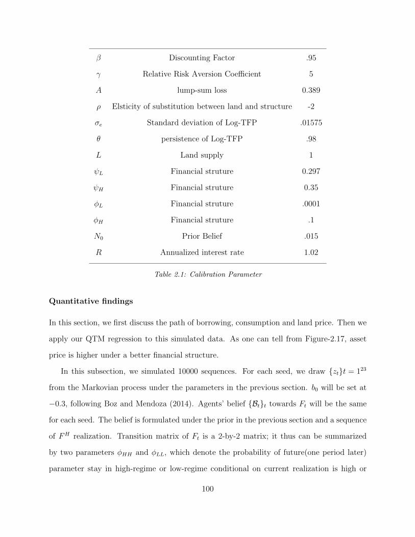
β Discounting Factor .95

γ Relative Risk Aversion Coefficient 5

A lump-sum loss 0.389

ρ Elsticity of substitution between land and structure -2

σe Standard deviation of Log-TFP .01575

θ persistence of Log-TFP .98

L Land supply 1

ψL Financial struture 0.297

ψH Financial struture 0.35

φL Financial struture .0001

φH Financial struture .1

N0 Prior Belief .015

R Annualized interest rate 1.02

Table 2.1: Calibration Parameter

Quantitative findings

In this section, we first discuss the path of borrowing, consumption and land price. Then we

apply our QTM regression to this simulated data. As one can tell from Figure-2.17, asset

price is higher under a better financial structure.

In this subsection, we simulated 10000 sequences. For each seed, we draw ztt = 123

from the Markovian process under the parameters in the previous section. b0 will be set at

−0.3, following Boz and Mendoza (2014). Agents’ belief Btt towards Ft will be the same

for each seed. The belief is formulated under the prior in the previous section and a sequence

of FH realization. Transition matrix of Ft is a 2-by-2 matrix; it thus can be summarized

by two parameters φHH and φLL, which denote the probability of future(one period later)

parameter stay in high-regime or low-regime conditional on current realization is high or

100

low. I plot this transition matrix in Panel D of Figure-2.14.

For illustration purpose, we pick up a path of zt and plot out the path of consumption,

borrowing and asset price in Figure-2.14(implied β = 0.5745).As one can tell from Figure-

2.14, as optimism builds up, consumption increase, while borrowing keeps increase though

then converge to a steady state. Furthermore, the Land price keeps going up during the

whole period. Under some parametrization of “true” process, people borrow too much. This

over-borrowing is a result of non-rational expectation and will make the sudden stop more

damaging. I can tell that consumption excesses new steady state 7%, at the peak, then

converges to steady state quickly(less than ten periods). However, the land price keeps

increasing during the whole sample period.

Thus, we then calibrate an ARMA(2,2) process36 to match M2 growth of U.S., And we

will use equation-5 to solve out the price. Then we run QTM regression to estimate the effect

of Money growth onto inflation; we focus on income adjustment here, the results without

income adjustment have very close distribution. Under our baseline parameter, from our

10000 simulations, slope estimator β of QTM is 0.572, as plotted in Figure-2.16, where we

plot out the simulation distribution of β. As one can tell from Figure-2.16, our money loading

ranges from 0.54 to 0.6, significantly less than 1. Hence our mechanism and model can offer

an alternative explanation to collapsing of QTM.

2.6 Conclusion

In this article, we reviewed and discussed the historical performance of the Quantity The-

ory of Money(QTM). I re-evaluate the one-to-one relationship between money growth and

inflation. By adopting the same statistical and economic criteria as Lucas (1980), with a

much larger data set covering both a longer period and many more countries, we found QTM

36ARMA(2,2) is used just for a parsimonious setting. One can use an AR(2) process too.

101

Figure 2.16: Distribution of βt, 10000 simulation paths of zt

breaks in U.S, and this collapsing of QTM is universal.

It appears that the period 1955-1980 is the only period during which QTM fits data

well in most of our sample countries. It starts to break down when we go beyond this

period. Furthermore, the recent breaking down of QTM coincides with a process of financial

innovation.

To explain this breaking down for U.S, we use a money generating theory instead of money

demand. To be more precise, the loan is an important source of money generation. And we

decompose the loan structure of U.S market. I found real estate is the major collateral asset

of Households and Firms. I thus propose money chases after real estate, a bundle of final

goods and land. To confirm our judgment, we use a long historical data of nominal house

price and find that (long-run) growth of nominal house price co-moves with(leads) growth

of broad money more robustly.

I then propose a framework under which financial innovation can affect our estimation

of QTM. And as our quantitative exercise shows our model is capable of explaining the

collapsing of QTM.

102

2.7 Appendix

2.7.1 Data source, Cross-Country

I obtain different measures of money stock from various sources. The main data source

of cross country data is from the dataset offered by Schularick and Taylor (2012). They

also offer an extraordinary database recently: http://www.macrohistory.net/data/. The

original data sources, which I explored, are summarized as follows:

Norway: Historical statistics of Norge Bank 37. For M1/2, 1870-1919 are from Jan T.

Klovland, Monetary Aggregates in Norway 18192003, chapter 5, Page 208-210. 1919-2006 are

from Table a2a. Nominal and real GDP are from Table-c6-table5 and table6. For deflator,

data are taken from Table-c6-table7. Data from 1940-1945 are missing. For 2004-2015,

Statistics Norway(M1 and M2 are from Table-0825338 and Table-10945). Data of real and

nominal GDP from 2000-2015 are from Eurostat. CPI data from 1924(1864)-2015 are from

table 08184 of Consumption index, issued by Statistics Norway. After 1924, we use the

growth rate of CPI to represent inflation.

Switzerland: 1907-2006, M1/3 is from The monetary base and the M1, M2, and M3 mon-

etary aggregates, Swiss National Bank, 2007. Before 1907, we take the data from Schularick

and Taylor(2012) For Price, 1870-1992 are from H.1 of historical statistics of Switzerland

online. After that, we adopt CPI from Swiss Federal Statistical Office. For GDP, 1870-1913

are from Table Q.1a; 1914-2005 are from Q.16a, b; 1980-2016 are from Eurostat. From

1984-2016, data of M1/2/3 are available from the database of Swiss National Bank.

Sweden: Historical Monetary and Financial Statistics for Sweden, Volume 1-2, Sveriges

Riksbank. For 1872-2006, CPI and GDP deflator are taken from Table A8.1, Volume 1,

Page 443-447. M0/3 during 1846-2012 are taken from Table A7.2, and 7.3, Volume 1, Page

325-332, since No data on M1 was presented before 1999. After 2012, we use data offered

37http://www.norges-bank.no/en/Statistics/Historical-monetary-statistics/38data of M1/2 stops at Feb, 2015

103

by Statistics Sweden. GDP is taken from Table A4.3, Page 164-169 from 1872-2000. After

that, we take data from Statistics Sweden. CPI during 1980-2016 is taken from Statistics

Sweden(Consumer Price Index (CPI)/Living Cost Index, July 1914=100).

Australia: M1/3: 18701983 Page 5771 from David Pope, Australian Money and Banking

Statistics. M3 after 1960 is from Reserve bank of Australia(RBA, ID: DMAM3N), M1 after

1975 is from RBA(ID: DMAM1N), between 1960-1975, we use data from OECD. CPI from

1922-2016 from RBA(Table G1, GCPIAG)

U.S: Real and nominal GDP (M1, M2 stock) are available from the FRED database since

1947: I (1959: I). Before that growth rates on the real GNP and M1, M2 series constructed

by Balke and Gordon (1986). Since there is no M1 data until 1914, we use the growth rate

of money base to approximate the growth rate of M1 from 1871-1914.

U.K: M0/1/3/4/4x and nominal GDP is from Money creation in the modern economy,

by Michael Mcleay, Amar Radia and Ryland Thomas. Consumption price and Real GDP

data is from The UK recession in context what do three centuries of data tell us? by Bank

of England. After 1997, we use M4x(excluding intermediate other financial corporations) to

represent broad money index. According to Bank of England, “...modify the measurement of

UK M4 by excluding the money holdings of some OFCs in order to obtain a better measure

of those money holdings that are likely to be used as a medium of exchange.”

Spain: From 1870-1998, M1/2 and Broad index(Disponibilidades liquidas, similar to M2

definition of Fed). Table 9.16, Page697. Carreras and X. Tafunell (eds.), Estadisticas His-

toricas De Espana, Madrid 2005 http://www.fbbva.es/TLFU/dat/autores.pdf. After that,

we get them from IFS. 1936-1940 are missing for Money. Nominal GDP(El PIB a precios

corrientes) from 1870-2000, Table 17.7, Page 1339-1340. After that we can have GDP from

Eurostat(1995-2006). GDP deflator, from 1870-2000, Table 17.16(Deflactores implcitos del

PIB a precios de mercado y sus componentes de gasto). 1995-1997, we can use data from

OECD. After 1998, we use (M1/3)data from Table 1.13 from Banco de Espana.

104

Denmark: From 1995-2016, M1/3 are from Danmarks Nationalbank(1995-2013 from Ta-

ble DNM1KOR, after 2005 from table DNMNOGL). From 1970-1995, we use data from

OECD. Nominal Gdp is from Barro-Ursua Macroeconomic Data (2010). From 1971-2016, we

take from OECD. Real GDP (1995-2016) and Harmonized Index of Consumer Prices(2001-

2016) are taken from Eurostat. Monetary data before 1971 are from narrow(broad) monetary

index of Schularick and Taylor(2012)39.

Germany: (M0/M2, Price and output, Pre-1960) are from Rolnick and Weber (1997)40.

Then for M1/3 during 1969-1998, we take data from IFS, after 1999 from Deutsche Bundes-

bank(we add ”German contribution to the monetary aggregate M3 and its components in the

euro area ” with “Banknotes in circulation / Deutsche Bundesbank.” ). For real GDP and

CPI from 1971-2000, we use data from OECD. Then I use data from Deutsche Bundesbank.

Netherlands(M1/2/3), from 1982-2015, Table 5.4 from De Nederlandsche Bank. They

do not directly provide M1, M2. So we use the definition of Monetary stock according to

ECB: M1= Currency in circulation+Overnight deposits. M2= M1+Deposits with an agreed

maturity up to 2 years+Deposits redeemable at a period of notice up to 3 months41. For

pre-1982, we adopt data from Schularick and Taylor(2012).

France(M1/2) are from Banque De France-M1,242 after 1980, before which we adopt data

from Rolnick and Weber (1997).

Italy(M1, M2 plus/3): For the whole period, GDP index is taken from Alberto Baf-

figi(2011) Italian National Accounts, 1861-2011. M1/2, 1861-1939, Monetary aggregates

in Italy 1861-2014, Banca d’Italia. After 1999, we take data from Banca d’Italia. I con-

39They construct the monetary index by sum liability of the central bank, commercial banks and savingbanks, by using data from Hans Chr. Johansen(1986)

40As robust check we also used data from Schularick and Taylor(2012), they construct M1 based onDeutsche Bundesbank (1976), “Deutsches Geld- und Bankwesen in Zahlen 1876-1975”

41M3=M2+Repurchase agreements+Money market fund (MMF) shares/units+Debt securities up to 2years. This debt is restricted to liabilities of the money-issuing sector and central government liabilities witha monetary character held by the money-holding sector

42MI.M.U2.Y.V.M10.X.1.U2.2300.Z01.M.E.C.X and MI.M.U2.Y.V.M20.X.1.U2.2300.Z01.M.E.C.X3+-

105

struct M3(M1) by adding “Italian contribution to euro-area M3(M1) excluding currency”43

and “currency held by public”44. From 1940-1998, M145 Data is offered by Banca d’Italia.

M2plus46 offered by Banca d’Italia) was used before 1998 (Historic data offered by Banca

d’Italia). After 1998, we use M3.

For Canada, M1/2 series: M1 before 1952 is from Metcalf, Redish, and Shearer (1996)

after 1980 we use data from Statistics Canada, M2 before 1967 is from Metcalf, Redish, and

Shearer (1996). All data between can be downloaded from Statistics Canada. And Metcalf,

Redish, and Shearer (1996) offer monthly data; we convert the monthly series to the annual

frequency by taking value in December. GDP and GDP deflator data are from Statistics

Canada47.

43BAM-AGGM.M.1020001.M3XC.3.101.EMUBI4.SBI138.100044BAM-AGGM.M.1010001.AM01.0.101.WRDBI2.S0.EUR45SST-STSMB.M.M1ST.10146SST-STSMB.M.M2PLST.10147Table 380-0064

106

2.7.2 Numerical Solution

For completeness, we first derive equation-(1) to (6). Then we went through the solution

details.

L =∑t

βtU(ct)+λt[(qt + dt)st + bt + Lt − st+1qt − ct −bt+1

R]

+µt[bt+1

R+ φtqtst+1 + ψt]

First order conditions of ct, st+1 and bt+1 will be

U ′(ct) = λt

λtR

=µtR

+ EBt [βλt+1] ⇒ U ′(ct) = REBt [βU(ct+1)] + µt (A.1)

λtqt = EBt [βλt+1(qt+1 + dt+1)] + µtφtqt ⇒ qt =EBt [βλt+1(qt+1 + dt+1)]

U ′(ct)− φtµt(A.2)

Combine equation-(A.1) with budget constraint and binding borrowing constraint will have:

ct = min(U ′)−1(EBt [βRU ′(ct+1)]), ψt + φtqtst+1 + bt + ztg(1) (A.3)

For any period t, exogenous state variables are zt and Ft, endogenous state variable is

bt and st. Since market clear condition restricts st to be 1, we simply state that bt is the

only endogenous variable. Given any realization of exogenous state variables, there exists a

b, such that borrowing constraint will be binding if bt < b48.

Given any realization of zt, Ft, b and policy functions from last iteration(k), ck(z, F,B),

qk(z, F,B), and µk(z, F,B):

When bt ≥ b, borrowing constraint is loose, we denote the current case as Case.1. Con-

sumption is thus determined by the left branch of equation-A.3. If agent choose a bond

48It is possible that b =∞, so borrowing constraint will be binding regardless the realization of exogenousvariable

107

holding B′ next period, we denotes the consumption policy function as ct(zt, Ft, B′), which

will defined as following:

c1,t(zt, Ft, B′) = (U ′)−1(EBt [βRU ′(ck(zt+1, Ft+1, B

′))]) (A.5)

where (U ′)−1 is inverse function of U ′(.) and ck(z, F,B) is policy function from iteration

k. This policy function is defined on state variable space. It is worthy to point out that

c1,t(zt, Ft, B′) is not a policy function yet, since B′ is not a state variable, at least not for

period t. And when bt ≥ b, borrowing constraint is loose, thus µt(zt, Ft, B′) = 0. From

equation-(A.2), we can solve out the value of collateral asset given people choose bond

holding of next period to be B′ as below:

q1,t(zt, Ft, B′) =

EBt [βU ′(ck(zt+1, Ft+1, B′))(qk(zt+1, Ft+1, B

′) + dt+1)]

U ′(c1,t(zt, Ft, B′))(A.6)

where qk(z, F,B) is policy function from iteration k. dt+1 is dividend from land. And the

exception in equation-(A.5) and (A.6) are based on belief Bt towards zt+1 and Ft+1. And

q1,t(zt, Ft, B′) is an increasing function of the first and third input. Furthermore, bt can be

backed out through budget constraint if people choose bond holding of next period to be B′,

given st+1 = st = 1:

ct +B′

R= dt + Lt + bt ⇒

bt(zt, Ft, B′) = dt + Lt − ct(zt, Ft, B′)−

B′

R

Hence, for any zt and Ft, we define policy functions in iteration k + 1 for B ≥ b(zt, Ft) or

108

Case 1 as:

ck+11 (z, F,B) = c1,t(z, F, dt(z) + Lt(z)−Rct(z, F,B′)−RB)

qk+11 (z, F,B) = q1,t(z, F, dt(z) + Lt(z)−Rct(z, F,B′)−RB)

µk+11 (z, F,B) = 0

where c1,t(zt, Ft, B′) and q1,t(zt, Ft, B

′) are defined in equation-(A.5) and (A.6).

Otherwise, when bt < b, borrowing constraint is binding, we denote the current case

as Case 2. Thus value of collateral asset is thus determined by borrowing constraint-*.

Given agent choose a bond holding B′ next period, we denotes asset price policy function as

qt(zt, Ft, B′), which will defined as following:

q2,t(zt, Ft, B′) =

1

φt[−ψt −

B′

R] (A.7)

where both of φt and ψt are determined by Ft. And we substitute mu2,t = U ′(ct) −

EBt [RU ′(ct+1)] into asset pricing equation-A.2 to solve consumption, we will get:

c2,t(zt, Ft, B′) = U ′−1(

1

1− φtU′(ck(zt+1, Ft+1, B

′))(dt+1 + qk(zt+1, Ft+1, B′))

q2,t(zt, Ft, B′)

− φtRBt [RU ′(ck(zt+1, Ft+1, B′))]) (A.8)

where q2,t(zt, Ft, B′) is determined in Equation-A.8. Furthermore, according to equation-A.1:

µ2,t(zt, Ft, B′) = U ′(c2,t(zt, Ft, B

′))− EBt [RU ′(ck(zt+1, Ft+1, B′))] (A.9)

where (U ′)−1 is inverse function of marginal utility U ′(.), ck(z, F,B) and qk(z, F,B) are

109

consumption and asset price policy function from the kth iteration. And finally in follow-

ing formula, we back out the endogenous state variable bt at which given exogenous state

variables Ft, agent is to choose B′ as bond holding for next period.

From budget constraint:

bt(zt, Ft, B′) = dt + Lt − ct(zt, Ft, B′)−

B′

R

The policy functions for the k+1th iteration can be defined as following when borrowing

constraint is binding:

ck+12 (z, F,B) = c2,t(z, F, dt(z) + Lt(z)−Rct(z, F,B′)−RB)

qk+12 (z, F,B) = q2,t(z, F, dt(z) + Lt(z)−Rct(z, F,B′)−RB)

µk+12 (z, F,B) = µ2,t(z, F, dt(z) + Lt(z)−Rct(z, F,B′)−RB)

In the end, we need to define a b for each zt and Ft. As we know, b is the threshold, if

bt ≥ b agent stays unconstrained. In another words, b is the level at which agent will be

marginal binding: For any realization of zt and Ft, say zt = z, Ft = F , b(zt, Ft)49 is the

solution of

ck+12 (z, F, b) = ck+1

1 (z, F, b)

where cki (z, F, b), i = 1, 2 represents consumption policy function under case i. As our policy

functions converge, threshold level will converge too.

Furthermore, since we are forcing agents to choose B′ for next period, then we should

restrict the choice of B′ is a reasonable set. For example, for a borrowing constraint to be

bind, B′ < −ψt, or agent will face no restriction at all, even when the collateral has zero

49Since b will be different for different exogenous variables. Hence it is a function of zt and Ft.

110

Figure 2.17: Policy functions under different Financial structure parameters realization Ft, giveny = Y H

value.

The range of B′ is of course given by Equation-*. Under the constraint, B′ ≥ −ψt −

φtqtst+1 ≥ −ψt−φtqt. Given any realization of zt = z and FF , B′ ≥ −ψt−φtqi,t(zt, Ft, B′) ≥

−ψt − φtq1,t(zt, Ft, B′), the second inequality follows from Equation-A.2 with µ = 0. Or we

can present borrowing constraint as ψt + φtq1,t(zt, Ft, B′) +B′ ≥ 0, the left hand side of this

equation is increasing function of B′. The lower bound of B′ should be thus solved from

equation below:

ψt + φtq1,t(zt, Ft, Blower) +Blower = 0

Hence, we will restrict B′ ∈ [Blower,−ψt] and solve case 2. If backed bt stays below b, the

policy function serves as constraint branch. Similarly, we restrict B′ ≥ Blower when solving

case 1. If backed bt stays above b, the policy function serves as unconstrained branch. Since

bt are backed through budget constraints in both cases and consumption and borrowing is

lower in case 2, backed bt has no overlapping. I can patch these two branch together and

form the policy function for next iteration.

111

A numerical solution under parameter β = 0.96, R = 1.03, γ = 3, α = .2, φH(L) =

0.070(.05), ψH(L) = 0.2(.2), zH(L) = 1.1(.969), is displayed in Figure-2.17.

112

Chapter 3

Quantity Theory of Money is not a

Universal Rule: Evidence from

Monetary History of Thirteen

Countries

3.1 Introduction

The Quantity Theory of Money (QTM) is at the heart of Monetary Economics since its

birth. QTM is a long-run statement which provides that inflation rate will be the same with

the growth rate of Money in the long-run. Since Money has real effects in the short run,

we can only have QTM in the long-run or as a steady state equilibrium, for example Lucas

(1980) and Lucas (1996). QTM receives strong rigorous empirical supports since Lucas’

works. Lucas (1980) believes that QTM

“...possess[es] a combination of theoretical coherence and empirical verification shared

by no other propositions in Monetary economics. . . , . . . It is hard to imagine a nonvacuous

113

economic prediction obtaining stronger confirmation than that shown. . . This is the kind of

“empirical verification” of the quantity theory on which economists who assign it a central

theoretical role base most of their confidence.” (Page 1007, Lucas (1980))

There is no doubt that, at least since Friedman (1956), Lucas (1980) has been the most

influential restatement of the QTM for the elegance and strength of this empirical result. In

fact, Bob Lucas shows that, for US during 1955-1977, M1 growth and CPI inflation where,

when short-run movements had been reasonably filtered out, essentially one-to-one linked.

The co-movements between inflation and the growth rate of M1 were on a one-to-one basis.

Of course, the “Long-run” is not an empty title. The cross-country evidence, which shows

up in McCandless Jr and Weber (1995), uses 30 years (1960-1990) average annual inflation

rate and average (annual) growth rate of M2 across 110 countries. McCandless Jr and Weber

(1995) plots inflation rate against the growth of M2 and finds that these points line up near

perfectly along a 45-degree line. Lucas (1996) views this as a great success of QTM and

Monetary Economics:

“...The kind of monetary neutrality shown in this figure needs to be a central feature of

any monetary or macroeconomic theory that claims empirical seriousness...”

Long-run signal, in Spectrum Analysis, is equivalent to the signals with a range of low

frequencies (long periods), say the area around frequency ω = 0. Lucas (1980) uses a band-

pass filter (e.g.,Christiano and Fitzgerald (2003)) to extract (estimate) long-run signal from

raw data and then plots (1) (QTM) filtered growth of money against filtered inflation; (2)

(Fisher’s Effect) filtered growth of money against (filtered) T-bill rate. Lucas (1980) finds

that in both graphs points almost line up along a 45-degree line. As a result, QTM reveals

itself with direct and indirect evidence from Lucas (1980) its influence over inflation.

Researchers use several empirical methods to elaborate(estimate) the title “long run”.

A famous cross-country evidence to support QTM, which shows up in McCandless Jr and

Weber (1995), uses 30 years (1960-1990) average annual inflation rate and average (annual)

114

growth rate of M2 across 110 countries. McCandless Jr and Weber (1995) plots (average)

inflation rate against (average) growth of M2 and finds that these points line up near perfectly

along a 45-degree line. More recently, Benati et al. (2016) applies co-integration test to long

spanned dataset. H

From now on, we would like to refer this average of annual rate across some time span

as Temporal Approach.In contrast, Lucas (1980) uses a Frequency Approach to exploit sup-

porting time series evidence from U.S data. In the pioneering work of Lucas (1980), the

author uses a preliminary band-pass filter to extract (estimate) the long run signal (most

persistent part of) from the annual growth rate of M1, CPI and T-bill rate during 1953-1977.

However, does QTM stable across time? Friedman (1988) conducts a preliminary test

to check the relationship between Price and Money during 1977-1980s. The inflation rate,

realized or expected, stays relatively more stable than, and irrelevant to money growth (in

U.S). Along with several others, we also found that QTM is not robust after some date for

the US.

For example: “...For most of the last 25 years, the quantity theory of money has been

sleeping...” (Sargent and Surico (2011), Page 110).

“...in a later period, the relationship(between money and inflation) turns negative in

frequencies 20 years or higher.....”(Christiano and Fitzgerald (2003)). Additionally, this

relationship is not even robust across history. In this article, I will show QTM is not even

robust across countries.

Furthermore, the latest breaking of QTM seems to be a global pattern, though different

countries have different breaking dates and degrees. There are several proposed explanation,

say disinflation policy, fiat or commodity Standards. However, we cannot find positive

evidence to confirm these proposals.

This article, instead of trying to explain QTM, checks whether QTM ever holds across

time and countries. Put in other words, does Bob get lucky when he explores the data of U.S

115

during 1955-1977? Does QTM hold before 1955 in U.S? Does QTM hold for other countries

during 1955-1977? How is the performance of QTM across nations during during the years

before 1955 or after 1980?

In this article, I investigated historical data of 13 countries during a long time span,

mainly from the late-1880s or early 1890s to 2006. I truncated my data to avoid the late

financial crisis. I applied the original method of Lucas (1980) to the cases of these 13

countries. It turns out that the Quantity theory of Money is not a global pattern before

the 1950s. But during 1950s-1980, for most of the countries in my sample, the (Long-Run)

growth rate of money provides a good explanation of inflation. However, the growth rate

of money has nothing to do with the interest rate, except 1950s-1980 for almost all the

countries. Most importantly, the latest breaking down of QTM happens at a different time

for different country. For example, the breaking date for U.S is 1991 if I use M2 as my main

focus, while for most of the European countries, it is 1998.

Additionally, whether QTM breaks hugely depends on the measure of money I am using,

echoing the message from Lucas and Nicolini (2015). For example, if one focuses on M4

index for U.K, the QTM still holds. However, M2 and M1 version of QTM breaks for U.K.

Hence, it is reasonable to doubt whether QTM still holds for more general definitions of

money. However, this goes beyond this scope of this paper.

Concerning to the method, I adopt the original method of Lucas (1980) in the main

body of this article. As a robustness check, we also used bandpass filter like Christiano and

Fitzgerald (2003) and (rolling over) spectrum at like ?. For U.S and U.K, I also checked

time-varying VAR. I agree that idea of Lucas (1980) is to estimate the long-run signal

out of original data. However, the estimation of the spectrum at ω = 0 is notorious of

unstable property. For more details, one can refer to Sargent (1987), Hamilton (1994) and

Ltkepohl (2007)., can be viewed as a smoothing(filtering) method to estimate the most

persisting identifiable component(s) from raw data. One can also refer it as the long-run

116

trend. Furthermore, I do not have a criterion or would like to take a stand on how long

should be named to be “Long-run” 30 years? 40 years? For example, if we would like to

explore dataset of U.S is from 1948-2015(post-WWII period), 30 years or above will also

have the similar disadvantage of a spectrum estimation at ω = 0. Additionally, laying out

the gain and coherence estimators would be a misleading part. For example, for coherence,

though people may have used several kinds of window function adjusted it, high value of

this estimator tends to have a high variance1. And when people have high gain estimator,

we should not accept that QTM is still alive. Since QTM refers to a one-to-one relationship,

the gain should be far away from 1 if QTM holds.

Lucas (1980) uses an elementary band-pass filter to extract the long run signal from M1,

CPI and T-bill rate during 1953-1977(hereafter, as Frequency (domain) Approach2).

To make band-pass filter work and avoid Spurious regression3, Lucas (1980) stationarizes

the data by taking annual growth rate of the raw data of M1 and CPI.

I am not the first to arise whether QTM is alive or not. For example, ? uses spectrum

estimation and finds that QTM is not stable. Rolnick and Weber (1997) finds that correlation

between inflation and money growth was weaker during the standard Gold Period than

during the fiat standard. Sargent and Surico (2011) found that QTM does not work recently.

Sargent and Surico (2011) use time-varying VAR and the filter of Lucas (1980) to establish

the recent failure of QTM. However, Sargent and Surico (2011) used the filter of Lucas(1980)

with 16 quarters window length.

In this empirical paper, we will replicate the filter of Lucas (1980) and check whether

Quantity theorem of Money hold across countries and cross time. In Wang (2017), I mainly

1It worths to point out that ? applies a Mont Carlo Method to simulate the variance of gain and coherence.2One can view (stationary) data Yt∞t=0 as (1)(Time domain) Yt = α +

∑j φjεt−j or(2)(Frequency

domain) Yt = α+∫ π0a(ω)cos(ωt)dω+

∫ π0b(ω)sin(ωt)dω. Please notice that M1 and CPI are not stationary

process yet.3Since at least M1 is a I(1) process in theory: Mt = Mt−1 + εt where εt is the money injection by central

bank. One can easily test unit root in M1 and CPI too. Con-integration test, e.g., Benati et al. (2016) isanother way out.

117

focus on the data U.S case.

This article will be organized as follows; I will describe the empirical method, data, and

results in the first three sections. Then we will conclude and leave the explanations of this

collapse to future research.

3.2 Empirical Method

Following Lucas (1980), I will work on following (quarterly) data transformation:

Gm(t) = log(Mt)− log(Mt−4)

π(t) = log(CPIt)− log(CPIt−4)

Gy(t) = log(yt)− log(yt−4)

Where CPIt and yt stand for consumption Price index and real GDP at time t. And Mt

stands for monetary aggregate, which can be currency and reserve, M1, M2 even M3/4 for

some countries. Since the definitions of monetary indices are different among countries. I

will label monetary stocks as narrow or broad money.

Lucas (1980) uses an exponential decreasing sequence as filter coefficient to extract long-

run information. To be more precise, Let window function ωρ,L(n) with bandwidth L, for

n = 0, 1, 2, ..T

ωρ,L(n) =

ρ|n| |n| ≤ L

0 |n| > L

I will denote x(t) and xf (t) for t = 1, 2, 3, ..., T as raw and filtered data respectively. xf (t) =∑Ts=1 ωρ,L(t − s)x(s) = Ω(L)x(t). One can try different bandwidth and discounting rate of

118

this filter, to extract long run signal out of raw data4. And it is worth to note that here we

use zero padding technic, which is common in signal analysis: setting the missing data to

0. After fixing bandwidth and rho to be sixteen years and 0.95, I extract out the long-run

growth rate of monetary stock, inflation and real income. Then I would like to check how

long-run inflation correlates with the long-run (income-adjusted) growth of money.

During the period under investigation of Lucas (1980), the growth rate of real GDP can

be viewed as a stable series. However, during the long historical period, I am to explore,

the growth rate of income cannot be taken as given. And to take this varying pattern of

the growth rate of GDP into account, I need to adjust growth rate of real GDP or GNP,

especially for the European countries. For example, the average growth rate of GDP of Spain

is 6.7% during 1951-1975, but 2.9% at most during 1976-2006.

Following Lucas (1980), I plot the filtered growth rate of money or excess growth rate of

money against inflation rate. The excess growth rate is defined to be the part of the growth

rate of money exceeding the growth rate of real GDP.

Lucas (1980) implicitly adopts an eyeball metric to illustrate the nearly perfect linear

relationship between growth rate of money and inflation. This idea, interpreted by Sargent

and Surico (2011), can be boiled down to a test whether the coefficient before money growth

equals to one if we run a regression of monetary growth onto inflation:

π(t) = α + βGm(t) + ε H0 : β = 1 (3.1)

Before we move on into the estimation results, it is worthy to note that β = 1 does not

necessarily mean quantity theorem holds. One can easily scatter several points along the 45-

degree lines to get unite slope. But it is hard to conclude that these two are closely related.

4when the gain function concentrate on low frequency. Variation of filtered date comes from the low-frequency variance of original data series; See Sargent (1987) or Stoica and Moses (2005) for more details.

119

Quantity theorem of money requires more than β = 1. It requires that money should be the

dominating driving factor of inflation. Put it in another way, R2 of this regression should

be close to 1. And this is the reason why ? includes coherency. In spectrum analysis,

coherency can be understood to be the R2. However, coherency estimation without any

window adjustment will be one by definition. It is reasonable to doubt this measurement

even after adjustment. Hence, we prefer to implement a simple regression method in this

section. Next, I turn to discuss the empirical results, data is mainly from the dataset of

Schularick and Taylor (2012), Balke and Gordon (1986), Bank of England, Bank of Italy,

Bank Australia and European central bank.

3.3 Empirical Results

Before getting into details, we have a problem of varying monetary regime: from Gold stan-

dard to Bretton Woods system, from Brettonwoods to its breaking down. And as Rolnick

and Weber (1997) conclude, the correlation between money and inflation is weaker during

commodity standard than fiat standard. But Rolnick and Weber (1997) mainly adopt a

cross-country regression, and different countries have final dates of commodity money stan-

dard. And I find this weak correlation is a temporal pattern, not necessarily linked to the

commodity money standard: Weak correlation happens mainly before 1900. Even when

commodity standard got abandoned before 1900, weak correlation generally will continue

for most of the countries.

During the period I am to investigate, several countries adopt Inflation target policy, one5

will find that this seems to cause breaking down of narrowly defined money in these countries.

For example, according to Hammond (2012), Canada adopt it since 1991, UK 1993, Australia

1993, Spain 1994, Switzerland and Germany 1970. M1 of U.S lost its explanation power to

5For example, Teles, Uhlig and Valle e Azevedo (2016)

120

inflation after 19806, Which is within the period during which Fed adopt disinflation policy.

However, there are countries with breaking QTM before the change of monetary policy

change.

Recent Breaking down of QTM happens in U.S, Sweden, Netherlands (rarely exists),

Denmark, France (rarely exists), Switzerland (QTM is a recent pattern), Australia and

Canada.

However, it is hard to conclude that QTM went asleep after some specific year, say 1984

for U.S. (1) Pattern breaking date depends on the window length we are using. Put in

another word; exact breaking date may be not robust to window length. (2)The monetary

stock is not well defined. There are dates before which M1 works, after which M1 does not

but M2/3/4 takes over.

This finding has a negative implication for policy recommendation. It does not matter

whether QTM is alive or not. Even if QTM is still alive, one does not have a stable and

robust measure to implement QTM. Concerning to learning or predict future inflation rate,

people do not have a public signal now.

In this section, we are using 16 years as bandwidth, and 0.95 as discounting rate, in

honor of Lucas (1980). In the graphs in appendix, I will color the point during different

periods; one will find that QTM is not a universal phenomenon. Whether QTM holds or

not is irrelevant with whether country implements fiat money or not7.

3.3.1 U.S.A

In Figure-3.1, with a much longer data set, from 1871-2008. I plot the growth rate of M1

and M2 against inflation rate in the upper panel. Down panel gives the pattern with income

adjustment. I label five different periods with different colors: 1871-1931(commodity stan-

6One will conclude different breaking date with a different filter. For example, using Lucas’ filter withdifferent window length.

7In an appendix available upon request, I also implement Fast Fourier Analysis and time-varying Var.

121

Figure 3.1: Filtered Growth rate of Money stock against Inflation rate, U.S

dard), 1932-1950(after abandoning commodity standard), 1951-1980(Lucas period), 1981-

2002 (Breaking-down period), and 2003-2006 (Pre-crisis).

As we can tell from the figure, the relationship between growth rate of M1 and inflation,

no matter controlling the growth of income or not, is nearly perfect. When we compare

the upper panel graphics with the ones in down panel, one can tell that for the case of U.S

that controlling the growth rate of income improves the fitting of QTM. However, adjusting

income will not save QTM from recent breaking down.

Growth rates of M1 and M2 co-moves with inflation perfectly during Lucas Period. With-

out controlling real income, β and R2 are 0.937(1.2), 0.88(.81), for M1(2). With income ad-

justment, β and R2 will become 0.771(0.967) and 0.97(0.96) for M1(2). Additionally, Lucas

period 1951-1980 is the period during which monetary indexes move closely with inflation

in most countries. Since I am using filtered data to run this regression, it is hard to use

standard deviation to determine whether we can reject hypothesis β = 1 or R2 = 1. I adopt

122

an ad-hoc criterion here, we used β = 0.7, R2 = 0.8 as a benchmark8.

More surprisingly, during 1932-1954, the growth rate of M1 has no explanation power to

inflation (β = −0.17, R2 = 0.07). And this powerless fact cannot be contributed to the Great

Recession since M1 starts not to explain inflation variation during several years previous to

1929. One can tell that during the same period, more broad indexes are valid after controlling

income growth (β = .91, R2 = 0.76). QTM failed for M1 completely. However, it is hard

to believe during 1932-1950, M2 plays a role in transactions. This is the reason why Wang

(2017) focuses on M2 for U.S.

During 1871-1931, if one would like to explore more on monetary standard: explaining

powers of M1 are different during this two sub-period (β = 0.29 for 1872-1899, and 0.91

for 1900-1931), difference persists even after controlling the real income. Additionally, M2

outperforms M1, especially after controlling income. But one will find the fitting of M2

during pre-1900 is still worse than 1900-1931. It is also worth to note that with different

bandwidth, it is possible to find different breaking date. For example, when we use 16

years as bandwidth, QTM break around 1991, while Sargent and Surico (2011) found QTM

break around mid-1980 by using four years as bandwidth and much lower R2 of the QTM

regression.

3.3.2 Australia

In Figure-3.2, I plot the growth rate of M1 and M2 against inflation in the upper panel.

Income adjustment cases are laid out at the down panel. I divide the case of Australia into

four periods, 1874-1931, 1932-1954, 1955-1980, 1981-1992, and 1993-2006. I have 1955-1980

as a period is to fit Lucas (1980). And I choose 1931 to be another threshold is because U.K

abandons commodity standard at 1931 according to Rolnick and Weber (1997). Additionally,

1993 is the year when Australia adopt Inflation target policy according to Hammond (2012).

8Or be more precise β should not stay too large either, we set β < 1.4, so 1β < 0.7

123

Figure 3.2: Filtered Growth rate of Money stock against Inflation rate, Australia

For Australia, M1 works well during 1955-1980, all points during this period lie along

the 45-degree line, except M2 during 1955-1559. But during 1932-1954, the one-to-one

relationship goes away no matter whether we control income and what monetary index one

would like to use. Hence, during 1932-1954, I conclude that inflation is robustly un-correlated

with money growth. If one would like to explore more, one will find from 1945-1950, the

correlation between inflation and money growth is negative.

Concerning to 1874-1931, one will again find that the “poor” performance of money

during commodity standard can be contributed to years previous to 1900: β and R2 for

M1 are 0.6352 and 0.97723 after 1900, while they are 0.27 and 0.097 before 1900. M2 has

a similar pattern: poor during years pre-1900(β = 0.33, R2 = 0.58), fits better from 1900-

1929(β = 0.98, R2 = 0.87), then deteriorates during 1930-1954, start to work during later

half of 1955-1980 and 1981-2006. On the other hand, M1 lost its explanation to inflation after

124

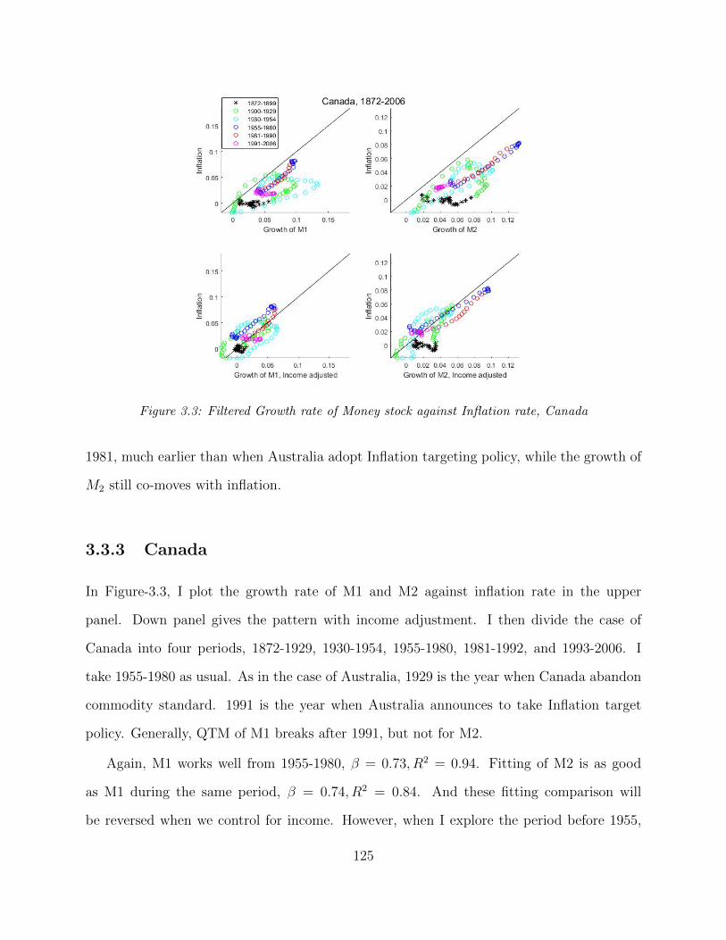
Figure 3.3: Filtered Growth rate of Money stock against Inflation rate, Canada

1981, much earlier than when Australia adopt Inflation targeting policy, while the growth of

M2 still co-moves with inflation.

3.3.3 Canada

In Figure-3.3, I plot the growth rate of M1 and M2 against inflation rate in the upper

panel. Down panel gives the pattern with income adjustment. I then divide the case of

Canada into four periods, 1872-1929, 1930-1954, 1955-1980, 1981-1992, and 1993-2006. I

take 1955-1980 as usual. As in the case of Australia, 1929 is the year when Canada abandon

commodity standard. 1991 is the year when Australia announces to take Inflation target

policy. Generally, QTM of M1 breaks after 1991, but not for M2.

Again, M1 works well from 1955-1980, β = 0.73, R2 = 0.94. Fitting of M2 is as good

as M1 during the same period, β = 0.74, R2 = 0.84. And these fitting comparison will

be reversed when we control for income. However, when I explore the period before 1955,

125

Figure 3.4: Filtered Growth rate of Money stock against Inflation rate, Switzerland

namely 1930-1954, inflation react insensitively to money growth (M1 and M2) no matter

whether I control for income or not.

During the area of the commodity standard, messages are mixing: During the years

before 1900, it is hard to conclude that inflation moves with the growth rate of money in a

one-to-one way, no matter whether we control income or not, the R2 are all less than 0.2.

The situation of 1900-1929 improves a little: inflation starts to react to changing growth

rate of money aggregate (M1 and M2), but still not in a one-to-one fashion.

Furthermore, for M2, there is no significant break at 1991, which is the year Canada

adopt inflation targeting policy. The breaking happens around 1997.

3.3.4 Switzerland

In the case of Switzerland, it is important to adjust the growth of income, especially for the

period after 1946 as shown in Figure-3.4. No index except excess growth rate of M2 can fit

inflation well. And M2 only starts to work after 1946. Switzerland is a little different from

126

Figure 3.5: Filtered Growth rate of Money stock against Inflation rate, U.K

all the other countries I investigate: (1) it abandons gold standard after 2000; (2) QTM is a

recent pattern for Switzerland and still holds. Switzerland is a perfect counter example to

the argument in favor of monetary standards.

Hence, I view Switzerland as a counterexample to statement of Rolnick and Weber (1997).

The weak correlation between money and inflation is not a necessary result of commodity

standard. Instead, the weak correlation seems to be a temporal pattern specific to the years

pre-1900. Since 2000 is close to the end of our data sample, it is hard to conclude any result

for fiat money standard in this case.

M1 does not work for Switzerland all the time, except when one would like to count the

fitting during 1900-1945 as a small success(β = 0.88, R2 = 0.45). On the other hand, it seems

to be safe to state that M2 after adjustment works well after 1946 until 2000. Furthermore,

for Switzerland QTM (controlled for income) is a recent pattern, which did not exist before

that.

3.3.5 U.K

U.K is the last country I investigate with filtering the whole sample, because of WWII, the

economy may fall under a different regime, prices may not be able to move freely during some

127

period. It will not give us too much hints on how money works. Wartime is an extreme case

for the economy: Government needs to issue a lot of money to finance their war, and this fiat

money is not backed by any commodity. People are afraid of government default, which is

pretty common phenomenon during the wartime. Then inflation will increase dramatically.

But this is not a confirmation of purchasing power of money, but a story of trust. For U.K,

I divide the whole sample into six pieces: 1870-1899, 1900-1931, 1932-1952,1953-1980,1981-

1990 and 1991-2006 as shown in Figure-3.5. 1931 is the year when U.K abandon commodity

standard, 1953 gives the best fit for QTM during the Lucas Period, and 1991 is when U.K

adopt Inflation target policy.

For United kingdom, generally speaking, quantity theorem works well, except 1932-1952

and recent breaking. For 1932-1952, as we discussed, this can be a result of the war. And

more interesting, the recent breaking down of QTM can be saved by using a broader monetary

index, M4.

As we found in other countries, inflation reacts to money growth in a detached pattern

during pre-1900 years, values of β of M1 and M2 are around 0.3. But if one gets into 1900-

1931, both β go up to 0.9. And during 1900-1931 inflation moves more closely with money

growth than the period 1953-1993, if one does not control income growth. However, fittings

get worse during 1932-1952.

I choose 1991 as a separating point is because U.K officially adopts inflation target after

1993. As one can tell from figure that the breaking of QTM locates around 1991, if one

chooses a narrow monetary measure, say M0 or M1. However, QTM of M4 cannot be counted

as broken if one is willing to abandon the sample period after 2006, following Sargent and

Surico (2011) to avoid the latest financial crisis. For M4, β = 0.80, R2 = 0.97 after controlled

for income.

In sum, one will find positive historical evidence of QTM for U.K, and it is still alive if

128

Figure 3.6: Filtered Growth rate of Money stock against Inflation rate, Germany

we adopt broad monetary index9.

3.3.6 Germany

Since Germany got involved in two World Wars, I decide to divide the sample into pre-1900,

1900-1913(commodity standard), 1926-1938(between WWI and WWII, no hyperinflation

period, which locates 1921-1924), 1952-1980(Lucas period), 1981-2006 as shown in Figure-

3.6.Germany abandoned the commodity standard in 1913. I filter commodity standard area

as a whole piece and color pre-1900 and post-1900(1900-1913) by different colors. 1952-2006

are also filtered together but colored differently. Period 1926-1938 is filtered alone, and the

hyperinflation period is excluded from my sample.

Without controlling growth or income, neither of the monetary indexes can explain fluc-

9It does not matter we adopt M4 or M4(x) during 1998-2006 since the growth rate of two indexes arepretty close.

129

tuation of inflation. For the case of M1, β attains 0.28 during 1884-1899, and stay at the

level of 0.12 − 0.16 till 2006. For M3, situation is similar, the maximum β = 0.26. If one

would like to insist on QTM without income adjustment, I have to conclude QTM never

(rarely) exists in Germany.

For comparison of pre-1900 and after-1900, a contrast to what happens in other countries,

during years pre-1900, M1 and M3 fit better than during 1900-1913.

When one controls income growth, one will find that Lucas period is the only period

during which inflation lies closely to M1 growth (β = 0.81, R2 = 0.86). After 1981, QTM

breaks down for M1 (β = −0.48, R2 = 0.34). Furthermore, there is a regime change in

Germany during 1952-2006. While M1 works well during Lucas period(1952-1980), the

explanatory power of M3 is not as strong as M1 during the same time (R2 = 0.72). However,

the situation got reversed after 1980: M3 has better fitting after 1980 (β = 0.7, R2 = 0.9),

while M1 got divergent with inflation. Since 1970 is the year Germany adopt Inflation target

policy, one can also divided the sample into pre-1970 and post-1970, but it is hard to conclude

that there is a structure break at this year.

3.3.7 Italy

Italy is a role model for Quantity theorem of Money. And there is even no breaking down of

QTM, at least if one restricts herself into the period before crisis as shown in Figure-3.7, as

this and other papers for all of the samples. I filtered two pieces of data sample separately:

1881-1939, 1952-2006. Then I further use different colors to label different periods: 1881-

1899, 1900-1939, 1952-1980, 1981-1998(before-Euro), and 1999-2006.

Italy abandons commodity standard on 1935. Since this year is close to WWII period, I

decide to investigate 1881-1939 as a whole piece for Italy. However, the result here is robust,

if one separates the sample at 1935. I further use two different color two eras of 1881-

1939: pre-1900 and 1900-1939. As one can tell from Figure 7, generally relationship between

130

Figure 3.7: Filtered Growth rate of Money stock against Inflation rate, Italy

money and inflation is weak during the years pre-1900 (without controlling income R2 for

M1(M3) is 0.6(0.68) before 1900, 0.85(0.95)after 1900. similar patterns show up when one

controls income). This is in line with my previous findings: so-called weak correlation during

commodity standard is a time-specific pattern, only happens before 1900. Furthermore,

M1/3 after income adjustment fits inflation during 1900-1939(for M1, β = 0.84, R2 = 0.95)

as well as 1952-1980(for M1, β = 1.2, R2 = 0.97). Hence, it is difficult to contribute QTM

to fiat money standard.

During 1952-1980 and 1981-1998, the growth of M1 or M3 correlated with inflation well,

and almost perfectly when one is willing to control the growth of income. During Lucas

period (1952-1980), income-controlled M1 and M2 works well for inflation(β = 1.2, 0.8 and

R2 = 0.97, 0.95). For Italy, the popular breaking down of QTM1 does not happen β =

0.75, R2 = 0.9, but explanation of M2 does decrease: β = 1, R2 = .96 during 1981-1998,

while β = 0.61, R2 = 0.99 during 1999-2006.

To sum up, everything works well until late 1990s, before the establishment of Euro. M2

131

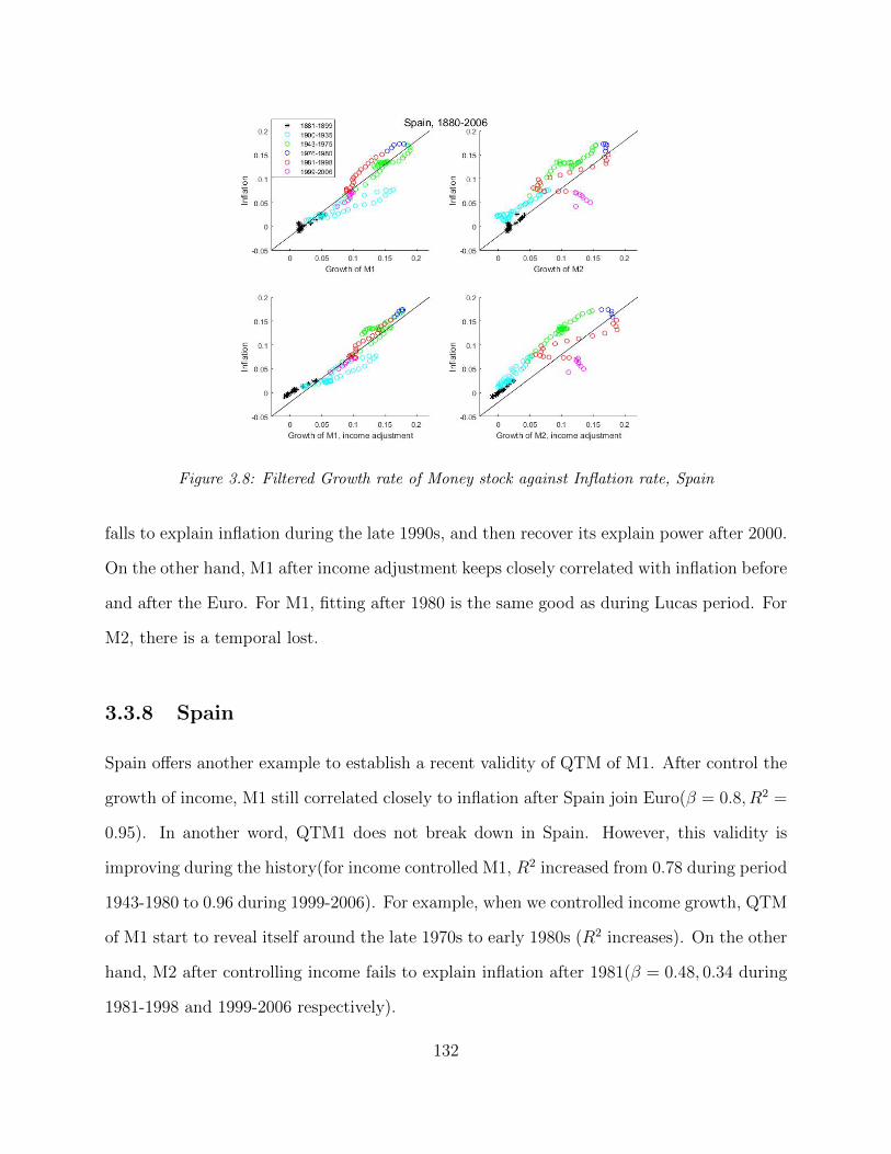
Figure 3.8: Filtered Growth rate of Money stock against Inflation rate, Spain

falls to explain inflation during the late 1990s, and then recover its explain power after 2000.

On the other hand, M1 after income adjustment keeps closely correlated with inflation before

and after the Euro. For M1, fitting after 1980 is the same good as during Lucas period. For

M2, there is a temporal lost.

3.3.8 Spain

Spain offers another example to establish a recent validity of QTM of M1. After control the

growth of income, M1 still correlated closely to inflation after Spain join Euro(β = 0.8, R2 =

0.95). In another word, QTM1 does not break down in Spain. However, this validity is

improving during the history(for income controlled M1, R2 increased from 0.78 during period

1943-1980 to 0.96 during 1999-2006). For example, when we controlled income growth, QTM

of M1 start to reveal itself around the late 1970s to early 1980s (R2 increases). On the other

hand, M2 after controlling income fails to explain inflation after 1981(β = 0.48, 0.34 during

1981-1998 and 1999-2006 respectively).

132

Spain adopts disinflation policy after 1994 according to Hammond (2012). And 1994 is

too close to Euro, if there is a structured break, it is hard to determine whether it is because

of Euro or disinflation policy. Like other European countries, our empirical results(not

presented here) show that if we only use data before Euro, namely focusing on data before

1998 only, there will be no breaking of Quantity theorem of Money for M2 either.

During 1881-1899, after we control growth rate of income, M1 and M2 work well to

explain inflation(without income adjustment β = 0.7(1.07), R2 = 0.8(0.75) for M1(M2)).

Then M1 begin to be not sufficient to move inflation around(β = 0.58(0.46) with(out) in-

come adjustment), M2 took over the power during 1900-1935(β = 1.2(0.8) with(out) income

adjustment). Generally, 1881-1935 is not a bad period for QTM.

During 1943-1975, I divide the sample into pre-1975 and post-1975 is because it is natural

to think Spain went through a regime change after Francisco passing away.

To sum up, for Spain, the message of QTM is mixing as shown in Figure-3.8. For M1,

it still works, especially after adjusting income growth. However, M2 seems to get divorced

with inflation after 1991. But as we discussed earlier, this breaking down depends on whether

we take the time after Euro into account.

3.3.9 France

I divide France into 1881-1899 (Pre-1900), 1900-1913(1900-Pre-WWI), 1922-1938(After WWI),

1946-1954(after WWII), 1955-1980(Lucas Period), 1981-1998 and 1999-2006 as shown in

Figure-3.9. France abandons commodity standard on 1936, which is too close to WWII, so

we group this year into 1922-1938. I filter Pre-1913, 1922-1938, and post-1946 separately.

Generally speaking, we cannot find a robust relationship between inflation and growth

of money. One may find that QTM reveals itself during the early part of 1981-1998, leaving

alone the breaking down during the later half. But generally speaking, it is even hard to

conclude that monetary index has ever correlated with inflation in a robust way in France.

133

Figure 3.9: Filtered Growth rate of Money stock against Inflation rate, France

Figure 3.10: Filtered Growth rate of Money stock against Inflation rate, Denmark

134

3.3.10 Denmark

There is no obvious time division for Denmark; we mainly divide Denmark into Pre-WII and

After WWII period. I filter these two pieces separately; one is from 1886 to 1938, one is from

1951-2006. Then we label different subsamples with different colors: 1886-1899, 1900-1913,

1914-1938, 1951-1980, 1981-1998 and 1999-2006 as shown in Figure-3.10. I do not have a

specific reason to group them in this way; I simply follow the case of Germany. I filter data

during 1886-1938 and 1951-2006 separately.

Quantity theorem of money holds perfectly during 1900-1938. Weak correlation still

applies to the pre-1900 period. The performance of M1 becomes bad after 1938. The

relationship between M3 and inflation is still there, though deteriorates. The breaking

happens during late-1990 depends on whether we sample in years after 2000. There is a

breaking down of QTM after 1999, for both M1 and M2.

During 1886-1899, the scatty plot is a common pattern across countries: Inflation is only

weakly correlated with money growth. After entering the 20th century, money starts to

reveal its power onto inflation. During 1900-1913 and 1914-1938, inflation is nearly perfectly

correlated with the growth of M1/3: Before 1900, M1(M3) β equals 0.28(0.38) if we do not

control the income. After 1900, β of M1(M2), is around 0.7.

However, after WWII, inflation got divorced with M1, even during 1951-1980(Lucas

period),β = 0.92 but R2 = 0.64. During 1951-1980 and 1981-1991, we have years during

which inflation fluctuate by its own without varying M1 growth. But M2 works after 1951

until late-1990(R2 = 0.77, 0.97). This kind of regime change happens in Germany too: before

a certain year, M1 works, but not after that date. M2 take over M1 after the threshold.

Broad money takes over.

135

Figure 3.11: Filtered Growth rate of Money stock against Inflation rate, Netherlands

3.3.11 Netherlands

Netherlands abandon commodity standard on 1936 and adopt disinflation policy on 1999.

1999 is a specific date for European countries. So we try to label this year out for all

European countries. For Netherlands, we separately filter two pieces of data: 1901-1948

and 1949-2006, then labor sub-samples with different colors. In the end, we have 1901-

1913 (Pre-WWI), 1914-1936 (Commodity standard), 1937-1948 (WWII), 1949-1980(Lucas

period), 1981-1998(before Euro) and 1999-2006. I filtered three pieces of sample separately:

pre-WWII, WWII and post-WWII. The reason of separating WWII from other sample is be-

cause that though Netherlands had proclaimed neutrality when war broke out in September

1939, just as it did during the World War I, it was still invaded by Germany in 1940.

Quantity theorem of money never exists in Netherlands, no matter we use M1 or M2,

control income or not. The relationship between the growth of money and inflation was

never close to one-to-one, though they move together closely.

During pre-WWII area, one can tell from Figure-3.11, the relationship between money

136

and inflation during these years are very similar. Inflation reacts to the growth of M1 and

M2 similarly. And inflation reacts to money in a very stable way: positive, but significantly

less than 1(the highest β is 0.5, M3 during 1914-1936). There seems to be another “quantity

theorem of money” in Netherlands, with coefficient less than 1 but closely co-movement

between money growth and inflation. Additionally, the performances of money are different10

during post-1900 than pre-1900: β = 0.35(0.36) for M1(M2) during pre-1900, β = 0.49(0.50)

during post-1900.

When one turns to 1949-1980, during the early stage, neither of varying M1 or M2 can

move inflation around, no matter we control income growth or not. Then inflation seems

to react to M1 in a one-to-one way for several years.Actually, this one-to-one relationship is

between 1955-1980, if we run regression just for this period, β = 0.77(0.72), R2 = 0.85(0.83)

for M1 with(out) controlling. After 1981, neither M1 or M3 growth co-moves with infla-

tion well, no matter whether I adjust income. It seems like QTM breaks down after 1981.

However, it rarely exists in Netherlands, except Lucas Period.

3.3.12 Norway

Norway abandons commodity standard on 1931, which is pretty close to our last year before

WWII, 1939. I group 1931 into our Pre-WWII sample. According to Hammond (2012),

Norway adopts disinflation policy on 2001. I separately filter data of Norway during Pre-

WWII and after-WWII. Then I further use different color to label different sub-samples:

1871-1899, 1900-1939, 1947-1960, 1961-1980, 1981-1998, and 1999-2006 as shown in Figure-

3.12. The reason I still choose 1999 is to keep consistent with other European countries,

results are robust to this threshold choice.

M3 works more robustly than M1 in Norway. Inflation reacts to the growth of M3 in

a one-to-one way generally. To be more precise, QTM works during 1900-1939, 1961-1980,

10The R2 are pretty similar.

137

Figure 3.12: Filtered Growth rate of Money stock against Inflation rate, Norway

1981-1998 and 1999-2006. On the other hand, M1 works during Lucas Period and 1900-1939.

During 1947-1960, the performances of these two indices get worse, no matter whether we

adjust income growth.

And it is worth to note that as most of other countries, money performs badly to explain

inflation variation during the year before 1900. This weak correlation hence should not be

taken as a characteristic of the commodity standard. Again, in Norway, commodity standard

got abandoned on 1931, thirty years later. Take M2 as an example, with(out) controlling

income, β = 0.72(0.74), R2 = 0.27(0.58) before 1900, β = 0.75(0.80), R2 = 0.88(0.89).

Generally, when I controlled income, M3 fits inflation well. In other words, QTM still

holds in Norway. Additionally, QTM holds for most of the European countries, if one stop

the data at 1998. And this is the reason why this article tries to separately label pre-1999

era out.

138

Figure 3.13: Filtered Growth rate of Money stock against Inflation rate, Sweden

3.3.13 Sweden

Sweden starts to adopt fiat standard from 1931. I divide the sample of Sweden into three

pieces and filter them separately pre-1938(pre-WWII), 1939-1950(WWII around), post-

WWII. I further label the whole sample by different colors: 1872-1899(pre-1900), 1900-1938

(pre-WWII), 1939-1950(WWII around), 1951-1980(Lucas period), 1981-1998(Pre-Euro), and

1999-2006. To reconfirm that weak correlation is not a result of the commodity standard, we

further label years before 1900 by using different colors with other years during 1900-1938.

Since Sweden keeps netural in two World Wars, I filter the sample together.

During 1872-1899, there is no significant correlation between inflation and money growth,

β = 0.07(0.88), R2 = 0.03(0.69) for M0(M3). Then M0 starts to positively correlated with

inflation from 1900, but less close than M3, β = 0.67(1.06), R2 = 0.61(0.87) for M0(M3)

during 1900-1938. During this period, M3 performs well to explain inflation. During 1961-

1980, both of M0 and M3 perform well, with income adjustment, β = 0.86(1.17), R2 =

139

0.92(0.98) for M0(M3).

WWII is notorious for invalidity of QTM, as we have already witnessed in other countries.

As one can tell from Figure-3.13, inflation keeps weakly co-move with money growth during

1939-1950, β = 0.085(0.19), R2 = 0.63(0.56) for M0(M3). Additionally, QTM breaks down

for Sweden at least since 1999.

3.4 Conclusion

In this paper, we are inspired by recent silent quantity theorem of money(QTM), especially in

U.S. I start out to check whether QTM is a robust relationship governing the co-movement

between money growth and inflation. I found evidence of recent breaking down of QTM

in U.S, confirming the finding of Sargent and Surico (2011) and Christiano and Fitzgerald

(2003). Moreover, we try to explore whether QTM is a robust pattern across the history of

U.S. The answer turns to be negative for M1 but positive for M2. In another word, QTM

is not a tight law across U.S history if one restricts itself to a pre-determined definition

of money. It implies that it is preferable to conclude which version of QTM breaks down

and more importantly which version of QTM still lives, echoing the message from Lucas

and Nicolini (2015). I then use long historical international data to confirm our finding in

U.S. By exploiting our international historical data; we found QTM is not robust across

countries either. There are countries where QTM exits and continues to exist. There are

countries where QTM exists for certain period. Furthermore, there are countries where QTM

rarely exists. I thus conclude that each country deserves a closer investigation to their own

monetary history to understand the recent universal collapse of QTM.

140

141

Bibliography

Abel, A. B. (1990): “Asset Prices under Habit Formation and Catching up with the

Joneses,” Working Paper 3279, National Bureau of Economic Research.

Aguiar, M., and M. Bils (2015): “Has Consumption Inequality Mirrored Income Inequal-

ity?,” American Economic Review, 105(9), 2725–56.

Ait-sahalia, y., J. A. Parker, and M. Yogo (2004): “Luxury Goods and the Equity

Premium,” The Journal of Finance, 59(6), 2959–3004.

Aiyagari, S., and M. Gertler (1999): “Overreaction of Asset Prices in General Equi-

librium,” Review of Economic Dynamics, 2(1), 3 – 35.

Attanasio, O. P., and L. Pistaferri (2016): “Consumption Inequality,” Journal of

Economic Perspectives, 30(2), 3–28.

Azariadis, C., L. Kaas, and Y. Wen (2016): “Self-Fulfilling Credit Cycles,” The Review

of Economic Studies, 83(4), 1364–1405.

Balke, N., and R. J. Gordon (1986): “Appendix B: historical data,” in The American

business cycle: Continuity and change, pp. 781–850. University of Chicago Press.

Bansal, R., D. Kiku, and A. Yaron (2007): “Risks For the Long Run: Estimation and

Inference,” .

142

Bansal, R., and A. Yaron (2004): “Risks for the Long Run: A Potential Resolution of

Asset Pricing Puzzles,” The Journal of Finance, 59(4), 1481–1509.

Barro, R. J. (2006): “Rare Disasters and Asset Markets in the Twentieth Century*,” The

Quarterly Journal of Economics, 121(3), 823–866.

(2009): “Rare Disasters, Asset Prices, and Welfare Costs,” American Economic

Review, 99(1), 243–64.

Benati, L. (2009): “Long Run Evidence on Money growth and inflation,” ECB working

paper.

Benati, L., R. Lucas, J. P. Nicolini, and W. Weber (2016): “International Evidence

on Long Run Money Demand,” (22475).

Benmelech, E., A. Guren, and B. T. Melzer (2017): “Making the House a Home:

The Stimulative Effect of Home Purchases on Consumption and Investment,” Working

Paper 23570, National Bureau of Economic Research.

Berger, A. N., and G. F. Udell (1990): “Collateral, loan quality and bank risk,”

Journal of Monetary Economics, 25(1), 21 – 42.

Bianchi, J., E. Boz, and E. G. Mendoza (2012): “Macro-Prudential Policy in a Fishe-

rian model of Financial Innovation,” Working Paper 18036, National Bureau of Economic

Research.

Bianchi, J., and E. G. Mendoza (2010): “Overborrowing, Financial Crises and ’Macro-

prudential’ Taxes,” Working Paper 16091, National Bureau of Economic Research.

Boldrin, M., L. J. Christiano, and J. D. M. Fisher (1997): “HABIT PERSISTENCE

AND ASSET RETURNS IN AN EXCHANGE ECONOMY,” Macroeconomic Dynamics,

1, 312–332.

143

(2001): “Habit Persistence, Asset Returns, and the Business Cycle,” The American

Economic Review, 91(1), 149–166.

Boz, E., and E. G. Mendoza (2014): “Financial innovation, the discovery of risk, and

the U.S. credit crisis,” Journal of Monetary Economics, 62, 1 – 22.

Brav, A., G. M. Constantinides, and C. C. Geczy (2002): “Asset Pricing with

Heterogeneous Consumers and Limited Participation: Empirical Evidence,” Journal of

Political Economy, 110(4), 793–824.

Breeden, D. T., M. R. Gibbons, and R. H. Litzenberger (1989): “Empirical Test

of the Consumption-Oriented CAPM,” The Journal of Finance, 44(2), 231–262.

Campbell, J. Y. (1999): “Chapter 19 Asset prices, consumption, and the business cycle,”

vol. 1 of Handbook of Macroeconomics, pp. 1231 – 1303. Elsevier.

Campbell, J. Y., and J. H. Cochrane (1999): “By Force of Habit: A Consumption-

Based Explanation of Aggregate Stock Market Behavior,” Journal of Political Economy,

107(2), 205–251.

Campbell, J. Y., and R. J. Shiller (1988): “Stock Prices, Earnings, and Expected

Dividends,” The Journal of Finance, 43(3), 661–676.

Chen, H., S. Joslin, and N.-K. Tran (2012): “Rare Disasters and Risk Sharing with

Heterogeneous Beliefs,” The Review of Financial Studies, 25(7), 2189–2224.

Chib, S. (2003): “MARKOV CHAIN MONTE CARLO METHODS: COMPUTATION

AND INFERENCE,” Handbook of Econometrics.

Christiano, L. J., and T. J. Fitzgerald (2003): “The Band Pass Filter*,” International

Economic Review, 44(2), 435–465.

144

Cogley, T., and T. J. Sargent (2008): “ANTICIPATED UTILITY AND RATIONAL

EXPECTATIONS AS APPROXIMATIONS OF BAYESIAN DECISION MAKING*,” In-

ternational Economic Review, 49(1), 185–221.

Constantinides, G. M., J. B. Donaldson, and R. Mehra (2002): “Junior Can’t

Borrow: A New Perspective on the Equity Premium Puzzle,” The Quarterly Journal of

Economics, 117(1), 269–296.

Davis, M. A., and J. Heathcote (2007): “The price and quantity of residential land in

the United States,” Journal of Monetary Economics, 54(8), 2595 – 2620.

Davis, M. A., and R. F. Martin (2005): “Housing, House Prices, and the Equity Pre-

mium Puzzle,” Staff working papers in the Finance and Economics Discussion Series.

Dittmar, R. F., F. Palomino, and W. Yang (2016): “Leisure Preferences, Long-Run

Risks, and Human Capital Returns,” The Review of Asset Pricing Studies, 6(1), 88–134.

Epstein, L. G., and S. E. Zin (1989): “Substitution, Risk Aversion, and the Temporal

Behavior of Consumption and Asset Returns: A Theoretical Framework,” Econometrica,

57(4), 937–969.

(1991): “Substitution, Risk Aversion, and the Temporal Behavior of Consumption

and Asset Returns: An Empirical Analysis,” Journal of Political Economy, 99(2), 263–286.

Fama, E. F., and K. R. French (1993): “Common risk factors in the returns on stocks

and bonds,” Journal of Financial Economics, 33(1), 3 – 56.

Friedman, B. M. (1988): “Lessons on Monetary Policy from the 1980s,” Journal of Eco-

nomic Perspectives, 2(3), 51–72.

Friedman, M. (1956): Studies in the Quantity Theory of Money. The University of Chicago

Press.

145

Hamilton, J. D. (1994): Time Series Analysis. Princeton University Press.

Hammond, G. (2012): State of the art of inflation targeting. Centre for Central Banking

Studies, Bank of England, 4 edn.

Hansen, L. P., and R. Jagannathan (1991): “Implications of Security Market Data for

Models of Dynamic Economies,” Journal of Political Economy, 99(2), 225–262.

Hansen, L. P., and K. J. Singleton (1983): “Stochastic Consumption, Risk Aversion,

and the Temporal Behavior of Asset Returns,” Journal of Political Economy, 91(2), 249–

265.

Jagannathan, R., and Y. Wang (2007): “Lazy Investors, Discretionary Consumption,

and the Cross-Section of Stock Returns,” The Journal of Finance, 62(4), 1623–1661.

Jermann, U., and V. Quadrini (2012): “Macroeconomic Effects of Financial Shocks,”

American Economic Review, 102(1), 238–71.

Kiyotaki, N., and J. Moore (1997): “Credit Cycles,” Journal of Political Economy,

105(2).

Kocherlakota, N. R. (1996): “The Equity Premium: It’s Still a Puzzle,” Journal of

Economic Literature, 34(1), 42–71.

Korinek, A., and E. G. Mendoza (2014): “From Sudden Stops to Fisherian Deflation:

Quantitative Theory and Policy,” Annual Review of Economics, 6(1), 299–332.

Kreps, D. M. (1998): “Anticipated Utility and Dynamic Choice,” Frontiers of Research in

Economic Theory: The Nancy L. Schwartz Memorial Lectures, pp. 242–74.

Kronencke, T. A. (2017): “Asset Pricing without Garbage,” The Journal of Finance,

72(1), 47–98.

146

Liu, Z., P. Wang, and T. Zha (2013): “Land-Price Dynamics and Macroeconomic Fluc-

tuations,” Econometrica, 81(3), 1147–1184.

Ltkepohl, H. (2007): New Introduction to Multiple Time Series Analysis. Springer.

Lucas, R. E. (1980): “Two Illustrations of the Quantity Theory of Money,” The American

Economic Review, 70(5), 1005–1014.

(1996): “Nobel Lecture: Monetary Neutrality,” Journal of Political Economy,

104(4), 661–682.

Lucas, R. E., and J. P. Nicolini (2015): “On the stability of money demand,” Journal of

Monetary Economics, 73, 48 – 65, Carnegie-Rochester-NYU Conference Series on Public

Policy Monetary Policy: An Unprecedented Predicament held at the Tepper School of

Business, Carnegie Mellon University, November 14-15, 2014.

Malloy, C. J., T. J. Moskowitz, and A. Vissing-Jorgensen (2009): “Long-Run

Stockholder Consumption Risk and Asset Returns,” The Journal of Finance, 64(6), 2427–

2479.

Mankiw, N., and S. P. Zeldes (1991): “The consumption of stockholders and nonstock-

holders,” Journal of Financial Economics, 29(1), 97 – 112.

Mankiw, N. G., and S. P. Zeldes (1990): “The Consumption of Stockholders and Non-

Stockholders,” Working Paper 3402, National Bureau of Economic Research.

McCallum, B. T., and E. Nelson (2010): “Chapter 3 - Money and Inflation: Some

Critical Issues,” vol. 3 of Handbook of Monetary Economics, pp. 97 – 153. Elsevier.

McCandless Jr, G. T., and W. E. Weber (1995): “Some monetary facts,” Federal

Reserve Bank of Minneapolis. Quarterly Review-Federal Reserve Bank of Minneapolis,

19(3), 2.

147

Mehra, R., and E. Prescott (1985): “The equity premium: A puzzle,” Journal of

Monetary Economics, 15, 145–161.

Parker, J. A., and C. Julliard (2005): “Consumption Risk and the Cross Section of

Expected Returns,” Journal of Political Economy, 113(1), 185–222.

Piazzesi, M., and M. Schneider (2016): “Chapter 19 - Housing and Macroeconomics,”

vol. 2 of Handbook of Macroeconomics, pp. 1547 – 1640. Elsevier.

Piazzesi, M., M. Schneider, and S. Tuzel (2006): “Housing, Consumption, and Asset

Pricing,” Working Paper 12036, National Bureau of Economic Research.

Piketty, T., and E. Saez (2003): “Income Inequality in the United States, 1913-1998,”

The Quarterly Journal of Economics, 118(1), 1–39.

Piketty, T., E. Saez, and G. Zucman (2016): “Distributional National Accounts:

Methods and Estimates for the United States,” Working Paper 22945, National Bureau

of Economic Research.

Rolnick, A. J., and W. E. Weber (1997): “Money, Inflation, and Output under Fiat

and Commodity Standards,” Journal of Political Economy.

Saez, E., and G. Zucman (2016): “Wealth Inequality in the United States since 1913:

Evidence from Capitalized Income Tax Data *,” The Quarterly Journal of Economics,

131(2), 519–578.

Sargent, T. J. (1987): Macroeconomic Theory (Economic Theory, Econometrics, and

Mathematical Economics Series).

Sargent, T. J., and P. Surico (2011): “Two Illustrations of the Quantity Theory of

Money: Breakdowns and Revivals,” American Economic Review, 101(1), 109–28.

148

Savov, A. (2011): “Asset Pricing with Garbage,” The Journal of Finance, 66(1), 177–201.

Schularick, M., and A. M. Taylor (2012): “Credit Booms Gone Bust: Monetary

Policy, Leverage Cycles, and Financial Crises, 1870-2008,” American Economic Review,

102(2), 1029–61.

Shephard, N. G., and A. C. Harvey (1990): “ON THE PROBABILITY OF ESTIMAT-

ING A DETERMINISTIC COMPONENT IN THE LOCAL LEVEL MODEL,” Journal

of Time Series Analysis, 11(4), 339–347.

Stoica, P., and R. Moses (2005): Spectral Analysis of Signals. Prentice Hall.

Teles, P., H. Uhlig, and J. Valle e Azevedo (2016): “Is Quantity Theory Still

Alive?,” The Economic Journal, 126(591), 442–464.

VissingJrgensen, A. (2002): “Limited Asset Market Participation and the Elasticity of

Intertemporal Substitution,” Journal of Political Economy, 110(4), 825–853.

Wang, X. (2015): “Simultaneous Estimation under DSGE Framework: Dis-inflation policy

against Relative Uncertainty,” Working Paper.

(2016): “Evolving Payment system: Re-reassess The Quantity Theory of Money,”

Working Paper.

(2017): “The Quantity Theory of Money: An Empirical and Quantitative Reassess-

ment,” Working Paper.

Weil, P. (1989): “The equity premium puzzle and the risk-free rate puzzle,” Journal of

Monetary Economics, 24(3), 401 – 421.

Whiteman, C. H. (1984): “Lucas on the Quantity Theory: Hypothesis Testing without

Theory,” The American Economic Review, 74(4), 742–749.

149

Yogo, M. (2006): “A Consumption-Based Explanation of Expected Stock Returns,” The

Journal of Finance, 61(2), 539–580.

(2008): “Asset Prices under Habit Formation and Reference-Dependent Prefer-

ences,” Journal of Business & Economic Statistics, 26(2), 131–143.

150