
ESSAYS IN DEVELOPMENT ECONOMICS
121
ESSAYS IN DEVELOPMENT ECONOMICS by Tongtong Hao A thesis submitted in conformity with the requirements for the degree of Doctor of Philosophy Department of Economics University of Toronto © Copyright by Tongtong Hao 2021
Transcript of ESSAYS IN DEVELOPMENT ECONOMICS

ESSAYS IN DEVELOPMENT ECONOMICS
by
Tongtong Hao
A thesis submitted in conformity with the requirements for the degree of Doctor of Philosophy
Department of Economics University of Toronto
© Copyright by Tongtong Hao 2021

Abstract
Essays in Development Economics
Tongtong HaoDoctor of Philosophy
Department of EconomicsUniversity of Toronto
2021
Since the beginning of its economic reform in 1978, China’s extraordinary economic growth has been ac-
companied by increased migration and rapid structural transformation – the reallocation of economic activity
from agriculture to nonagriculture. This significant labor reallocation and migration stemmed from a series of
institutional reforms and policies that significantly reduced labor market barriers. My thesis studies the impact of
changes in labor market barriers during China’s reform era.
Chapter 1 constructs measures of sectoral reallocation and geographical relocation of labor at the provincial
level for 1978-2015 resulting from a series of institutional reforms and policies that lowered labor market barri-
ers. I find that the structural transformation process was uneven across provinces. Agriculture-to-nonagriculture
worker reallocation began earlier and on a larger scale for coastal provinces. Since 1990, workers moving from
inland agriculture to coastal nonagriculture became an important source of nonagricultural labor growth.
Chapter 2 quantifies changes in barriers regarding sectoral reallocation and regional migration and studies
their impact on China’s economic growth over 1978-2015. I build a two-sector two-region general equilibrium
model focusing on labor market barriers both between agricultural and nonagricultural sectors and across coastal
and inland regions. I find that the 1982-2015 decline in labor market barriers contributed to an increase in output
of 26.5% in 2015. Despite this, there remain considerable gains for future improvement. In particular, eliminating
barriers from inland agriculture to coastal nonagriculture in 2015 could further increase output by 12%.
Chapter 3 presents the joint work with Ruiqi Sun, Trevor Tombe, and Xiaodong Zhu. Expanding on Chapter
2, we explore the effect of changes in capital market and trade frictions in addition to labor market barriers on
resource allocation. Employing a rich spatial general equilibrium model, we quantify the size and impact of mi-
gration barrier changes, capital barrier changes, and trade cost changes, to growth, regional income convergence,
and structural change in China over 2000-2015. While each contributed meaningfully to growth, migration policy
changes were central to China’s structural change and regional income convergence.
ii

Acknowledgements
For the work presented here, I am deeply indebted to my advisors, Loren Brandt, Gueorgui Kambourov, andXiaodong Zhu, for their patient guidance, tireless support, and continuous inspiration. I am grateful for everythingI have learned from them throughout the research process, about cultivating excellence, and pursuit of a betterself.
I have also benefited greatly from insightful discussions with many faculty at the University of Toronto. Isincerely thank Gordon Anderson, Diego Restuccia, Aloysius Siow, and all other participants of my CEPA andMacro brown bag seminars who took the time to offer constructive feedback. I would like to thank StephanAyerst, Baxter Robinson, Marc-Antoine Schmidt, and Jiaqi Zou for their friendship, motivation, mental support,and advice, which contributed greatly to the completion of this thesis.
Lastly, I would like to give special appreciation and thanks to my parents, Yingqi Hao and Guanghua Sun, andmy husband, Hao Zheng, for their endless support and encouragement in this pursuit over the years.
iii

I dedicate this thesis to my parents, for their unconditional love and support.
iv

Contents
Acknowledgements v
Contents v
List of Tables viii
List of Figures x
1 Measuring China’s Employment, Labor Reallocation, and Migration 11.1 Introduction . . . . . . . . . . . . . . . . . . . . . . . . . . . . . . . . . . . . . . . . . . . . . . 2
1.2 Background: Sectoral Reallocation and Geographical Migration . . . . . . . . . . . . . . . . . . 3
1.3 Measuring Sectoral Employment . . . . . . . . . . . . . . . . . . . . . . . . . . . . . . . . . . . 5
1.3.1 China Statistical Yearbook Official Employment . . . . . . . . . . . . . . . . . . . . . . 5
1.3.1.1 Official Yearbook Employment Data Construction . . . . . . . . . . . . . . . . 6
1.3.2 China Statistical Yearbook Alternative Employment . . . . . . . . . . . . . . . . . . . . 7
1.3.2.1 Alternative Yearbook Employment Data Construction . . . . . . . . . . . . . . 8
1.3.3 Census Employment . . . . . . . . . . . . . . . . . . . . . . . . . . . . . . . . . . . . . 9
1.3.4 Discussion and Choice of Employment Data . . . . . . . . . . . . . . . . . . . . . . . . 11
1.3.5 Sectoral Employment Trend by Regions . . . . . . . . . . . . . . . . . . . . . . . . . . . 14
1.4 Measuring Sectoral Labor Reallocation and Migration . . . . . . . . . . . . . . . . . . . . . . . . 15
1.4.1 Census Migration Data Construction . . . . . . . . . . . . . . . . . . . . . . . . . . . . . 17
1.4.2 Migration Trends and Patterns . . . . . . . . . . . . . . . . . . . . . . . . . . . . . . . . 19
1.4.3 Discussion on Sectoral Labor Reallocation and Migration Measures . . . . . . . . . . . . 26
1.4.3.1 Migrant Population and Migrant Workers . . . . . . . . . . . . . . . . . . . . . 26
1.4.3.2 Part-time Farmers . . . . . . . . . . . . . . . . . . . . . . . . . . . . . . . . . 26
1.4.3.3 Changing Hukou . . . . . . . . . . . . . . . . . . . . . . . . . . . . . . . . . . 28
1.5 Contribution of Switchers and Movers to Structural Transformation . . . . . . . . . . . . . . . . 29
1.5.1 Robustness Check: Other Measures . . . . . . . . . . . . . . . . . . . . . . . . . . . . . 30
1.6 Conclusion . . . . . . . . . . . . . . . . . . . . . . . . . . . . . . . . . . . . . . . . . . . . . . 32
1.7 Appendix . . . . . . . . . . . . . . . . . . . . . . . . . . . . . . . . . . . . . . . . . . . . . . . 34
1.7.1 List of Data Sources . . . . . . . . . . . . . . . . . . . . . . . . . . . . . . . . . . . . . 34
1.7.2 Additional Figure . . . . . . . . . . . . . . . . . . . . . . . . . . . . . . . . . . . . . . 34
v
Tongtong Hao
iii

2 Structural Transformation, Labor Reallocation, and Migration in China 352.1 Introduction . . . . . . . . . . . . . . . . . . . . . . . . . . . . . . . . . . . . . . . . . . . . . . 362.2 Model . . . . . . . . . . . . . . . . . . . . . . . . . . . . . . . . . . . . . . . . . . . . . . . . . 39
2.2.1 Production and Consumption . . . . . . . . . . . . . . . . . . . . . . . . . . . . . . . . . 392.2.2 Worker Reallocation and Migration . . . . . . . . . . . . . . . . . . . . . . . . . . . . . 402.2.3 Market Clearing . . . . . . . . . . . . . . . . . . . . . . . . . . . . . . . . . . . . . . . 41
2.3 Data Description and Parameterization . . . . . . . . . . . . . . . . . . . . . . . . . . . . . . . . 412.3.1 Data Description . . . . . . . . . . . . . . . . . . . . . . . . . . . . . . . . . . . . . . . 41
2.3.1.1 Output . . . . . . . . . . . . . . . . . . . . . . . . . . . . . . . . . . . . . . . 412.3.1.2 Employment . . . . . . . . . . . . . . . . . . . . . . . . . . . . . . . . . . . . 422.3.1.3 Sectoral Labor Reallocation and Migration . . . . . . . . . . . . . . . . . . . . 42
2.3.2 Data Summary . . . . . . . . . . . . . . . . . . . . . . . . . . . . . . . . . . . . . . . . 432.3.3 Labor Productivity . . . . . . . . . . . . . . . . . . . . . . . . . . . . . . . . . . . . . . 442.3.4 Calibration of Parameters . . . . . . . . . . . . . . . . . . . . . . . . . . . . . . . . . . 442.3.5 Mover/Switcher Costs Estimation . . . . . . . . . . . . . . . . . . . . . . . . . . . . . . 45
2.4 Quantitative Analysis . . . . . . . . . . . . . . . . . . . . . . . . . . . . . . . . . . . . . . . . . 472.4.1 Quantifying the Effect of Changes in Mover/Switcher Cost . . . . . . . . . . . . . . . . . 472.4.2 Quantifying the Remaining Labor Market Barriers . . . . . . . . . . . . . . . . . . . . . 48
2.5 Discussion on Alternative Mover/Switcher Measures . . . . . . . . . . . . . . . . . . . . . . . . 492.5.1 Part-time Farmers . . . . . . . . . . . . . . . . . . . . . . . . . . . . . . . . . . . . . . . 502.5.2 Changing Hukou . . . . . . . . . . . . . . . . . . . . . . . . . . . . . . . . . . . . . . . 512.5.3 Alternative Definition of Within-Region Mover/Switcher . . . . . . . . . . . . . . . . . . 53
2.6 Conclusion . . . . . . . . . . . . . . . . . . . . . . . . . . . . . . . . . . . . . . . . . . . . . . 572.7 Appendix . . . . . . . . . . . . . . . . . . . . . . . . . . . . . . . . . . . . . . . . . . . . . . . 59
2.7.1 Output Data . . . . . . . . . . . . . . . . . . . . . . . . . . . . . . . . . . . . . . . . . . 592.7.1.1 Nominal GDP and Real GDP Growth Rate . . . . . . . . . . . . . . . . . . . . 592.7.1.2 Deflator . . . . . . . . . . . . . . . . . . . . . . . . . . . . . . . . . . . . . . 60
2.7.2 Proof of Migration Share . . . . . . . . . . . . . . . . . . . . . . . . . . . . . . . . . . . 612.7.3 Construct Mover/Switcher Matrix . . . . . . . . . . . . . . . . . . . . . . . . . . . . . . 622.7.4 Additional Tables . . . . . . . . . . . . . . . . . . . . . . . . . . . . . . . . . . . . . . . 63
3 Migration Policy on Growth, Structural Change, and Inequality in China 663.1 Introduction . . . . . . . . . . . . . . . . . . . . . . . . . . . . . . . . . . . . . . . . . . . . . . 673.2 Sectoral Labor Reallocation, Migration, Structural Change, and Regional Income Convergence . . 69
3.2.1 Data . . . . . . . . . . . . . . . . . . . . . . . . . . . . . . . . . . . . . . . . . . . . . . 693.2.2 Factor Return Dispersion across Provinces and Sectors . . . . . . . . . . . . . . . . . . . 693.2.3 Regional Income Convergence and Structural Change . . . . . . . . . . . . . . . . . . . . 703.2.4 Sectoral Labor Reallocation and Migration in China . . . . . . . . . . . . . . . . . . . . 73
3.3 A Spatial Model of Trade, Labor Reallocation, and Migration . . . . . . . . . . . . . . . . . . . . 753.3.1 Individual Agents . . . . . . . . . . . . . . . . . . . . . . . . . . . . . . . . . . . . . . . 753.3.2 Production and Trade . . . . . . . . . . . . . . . . . . . . . . . . . . . . . . . . . . . . . 773.3.3 Incomes from Employment, Land, and Capital . . . . . . . . . . . . . . . . . . . . . . . 783.3.4 Capital Market Clearing Condition . . . . . . . . . . . . . . . . . . . . . . . . . . . . . . 793.3.5 Worker Mobility Across Provinces . . . . . . . . . . . . . . . . . . . . . . . . . . . . . . 79
vi

3.4 Quantitative Analysis . . . . . . . . . . . . . . . . . . . . . . . . . . . . . . . . . . . . . . . . . 803.4.1 Calibration of Time-Invariant Parameters . . . . . . . . . . . . . . . . . . . . . . . . . . 803.4.2 Size and Impact of Mover/Switcher Cost Reductions . . . . . . . . . . . . . . . . . . . . 81
3.4.2.1 Estimating Mover/Switcher Cost Changes . . . . . . . . . . . . . . . . . . . . 813.4.2.2 Quantifying the Effect of Mover/Switcher Cost Changes . . . . . . . . . . . . . 833.4.2.3 Comparison with Homothetic Preferences Model . . . . . . . . . . . . . . . . 853.4.2.4 Alternative Definition of Within-Province Mover/Switchers . . . . . . . . . . . 85
3.4.3 Effect of Lower Trade Costs . . . . . . . . . . . . . . . . . . . . . . . . . . . . . . . . . 873.4.4 Effect of Capital Wedges and Average Cost of Capital . . . . . . . . . . . . . . . . . . . 893.4.5 Decomposing Growth, Regional Income Convergence, and Structural Change . . . . . . . 92
3.4.5.1 Contributions to Growth . . . . . . . . . . . . . . . . . . . . . . . . . . . . . . 923.4.5.2 Contributions to Structural Change . . . . . . . . . . . . . . . . . . . . . . . . 933.4.5.3 Contributions to Regional Income Convergence . . . . . . . . . . . . . . . . . 93
3.5 Conclusion . . . . . . . . . . . . . . . . . . . . . . . . . . . . . . . . . . . . . . . . . . . . . . 943.6 Appendix . . . . . . . . . . . . . . . . . . . . . . . . . . . . . . . . . . . . . . . . . . . . . . . 96
3.6.1 Data . . . . . . . . . . . . . . . . . . . . . . . . . . . . . . . . . . . . . . . . . . . . . . 963.6.2 Proofs of Propositions . . . . . . . . . . . . . . . . . . . . . . . . . . . . . . . . . . . . 983.6.3 Supplementary Analysis . . . . . . . . . . . . . . . . . . . . . . . . . . . . . . . . . . . 101
Bibliography 107
vii

List of Tables
1.1 Yearbook Employment Data (million) . . . . . . . . . . . . . . . . . . . . . . . . . . . . . . . . 101.2 Census Samples Summary . . . . . . . . . . . . . . . . . . . . . . . . . . . . . . . . . . . . . . 121.3 Categorize migrants/movers, switchers and stayers . . . . . . . . . . . . . . . . . . . . . . . . . 171.4 Inter-province and Inter-region Migrant Fractions . . . . . . . . . . . . . . . . . . . . . . . . . . 191.5 Number of Employment, Switchers and Migrants (million) . . . . . . . . . . . . . . . . . . . . . 201.6 Characteristics of Workers with Agricultural Hukou . . . . . . . . . . . . . . . . . . . . . . . . . 221.7 Employment and Inter-County, Inter-Province Migration by Province . . . . . . . . . . . . . . . 231.8 Inter-County Migration Size and Provincial Share . . . . . . . . . . . . . . . . . . . . . . . . . . 241.9 Inter-Province Migration Size and Provincial Share . . . . . . . . . . . . . . . . . . . . . . . . . 251.10 Major Aggregated Migration Statistics (million) . . . . . . . . . . . . . . . . . . . . . . . . . . . 271.11 Ag-to-Nonag Switchers and Switcher&Movers (million) . . . . . . . . . . . . . . . . . . . . . . 281.12 Fraction of Hukou Changers among Urban Nonagricultural Workers . . . . . . . . . . . . . . . . 291.13 Contribution of Switchers and Movers to Structural Transformation (National) . . . . . . . . . . . 301.14 Contribution of Switchers and Movers to Structural Transformation (Regional) . . . . . . . . . . 311.15 Contribution of Switchers to Structural Transformation (including part-time farmers) . . . . . . . 321.16 Contribution of Switchers to Structural Transformation (including hukou changers) . . . . . . . . 33
2.1 Summary of Employment, Switchers and Migrants (million) . . . . . . . . . . . . . . . . . . . . 432.2 Number of Switchers and Migrants (million) . . . . . . . . . . . . . . . . . . . . . . . . . . . . . 442.3 Mover/Switcher Costs . . . . . . . . . . . . . . . . . . . . . . . . . . . . . . . . . . . . . . . . . 462.4 Decomposing the Effect of Mover/Switcher Cost Changes . . . . . . . . . . . . . . . . . . . . . 472.5 Decomposing the Remaining Mover/Switcher Costs . . . . . . . . . . . . . . . . . . . . . . . . . 492.6 Number of Part-time Farmers by Region (million) . . . . . . . . . . . . . . . . . . . . . . . . . 512.7 Modify the Migration Matrix for Part-Time Farmers . . . . . . . . . . . . . . . . . . . . . . . . . 522.8 Fraction of Hukou Changers among Urban Nonagricultural Workers . . . . . . . . . . . . . . . . 532.9 Including Hukou Changers as Migrants . . . . . . . . . . . . . . . . . . . . . . . . . . . . . . . 542.10 Number of Switchers and Migrants (million) . . . . . . . . . . . . . . . . . . . . . . . . . . . . . 552.11 Alternative Definition of Within-Region Migration . . . . . . . . . . . . . . . . . . . . . . . . . 562.12 Origin Worker Counts (million) . . . . . . . . . . . . . . . . . . . . . . . . . . . . . . . . . . . 642.13 Including Hukou Changers as Within-Region Mover/Switcher . . . . . . . . . . . . . . . . . . . 65
3.1 Sectoral Labor Reallocation and Migration in China, 2000-2015 . . . . . . . . . . . . . . . . . . 743.2 Model Parameters and Initial Equilibrium Values . . . . . . . . . . . . . . . . . . . . . . . . . . 813.3 Average Mover/Switcher Costs in China . . . . . . . . . . . . . . . . . . . . . . . . . . . . . . . 82
viii

3.4 Effect of Lower Mover/Switcher Costs, 2000-2015 . . . . . . . . . . . . . . . . . . . . . . . . . 833.5 Average Mover/Switcher Costs in China (Homothetic Preferences) . . . . . . . . . . . . . . . . . 863.6 Effect of Lower Mover/Switcher Costs, 2000-2015 (Homothetic Preferences) . . . . . . . . . . . 863.7 Intra-Provincial Worker Reallocation and Migration in China, 2000-2015 . . . . . . . . . . . . . 873.8 Average Migration Costs in China (Excluding Non-moving Switchers) . . . . . . . . . . . . . . . 883.9 Effect of Lower Migration Costs, 2000-2015 (Excluding Non-moving Switchers) . . . . . . . . . 883.10 Changes in Internal and External Trade Costs in China, 2002-2012 . . . . . . . . . . . . . . . . . 903.11 Internal and External Trade Shares of China, 2002-2012 . . . . . . . . . . . . . . . . . . . . . . 913.12 Effect of Lower Trade Costs, 2000-2015 . . . . . . . . . . . . . . . . . . . . . . . . . . . . . . . 923.13 Effect of Capital Market Changes, 2000-2015 . . . . . . . . . . . . . . . . . . . . . . . . . . . . 933.14 Decomposing China’s Growth, Income Convergence, and Structural Change . . . . . . . . . . . . 953.15 Average Capital Wedges Across Broad Regions and Sectors in China . . . . . . . . . . . . . . . . 1013.16 Robustness: Effect of Lower Mover/Switcher Costs, 2000-2015 . . . . . . . . . . . . . . . . . . 1033.17 Average Mover/Switcher Costs in China(k = 1.5) . . . . . . . . . . . . . . . . . . . . . . . . . . 1043.18 Average Mover/Switcher Costs in China (After Adjustment) . . . . . . . . . . . . . . . . . . . . 1053.19 Average Mover/Switcher Costs in China (Variant Registered Worker) . . . . . . . . . . . . . . . . 106
ix

List of Figures
1.1 Employment Data in the China Statistical Yearbook . . . . . . . . . . . . . . . . . . . . . . . . . 61.2 Agricultural Employment . . . . . . . . . . . . . . . . . . . . . . . . . . . . . . . . . . . . . . . 91.3 Compare Three Sectoral Employment Measures . . . . . . . . . . . . . . . . . . . . . . . . . . . 131.4 Map of Coastal and Inland China . . . . . . . . . . . . . . . . . . . . . . . . . . . . . . . . . . . 151.5 Employment Trends by Region . . . . . . . . . . . . . . . . . . . . . . . . . . . . . . . . . . . . 161.6 Nonagricultural Employment Share by Region . . . . . . . . . . . . . . . . . . . . . . . . . . . . 161.7 Number of Migrant Workers (million) . . . . . . . . . . . . . . . . . . . . . . . . . . . . . . . . 211.8 Compare Four Agricultural Employment Shares . . . . . . . . . . . . . . . . . . . . . . . . . . . 34
2.1 Sectoral Employment Share of China . . . . . . . . . . . . . . . . . . . . . . . . . . . . . . . . . 362.2 Labor Reallocation and Regional Migration . . . . . . . . . . . . . . . . . . . . . . . . . . . . . 372.3 Labor Productivity Trend . . . . . . . . . . . . . . . . . . . . . . . . . . . . . . . . . . . . . . . 452.4 Labor Productivity Gaps . . . . . . . . . . . . . . . . . . . . . . . . . . . . . . . . . . . . . . . 502.5 Trend of Ag-to-Nonag Switchers and Migrants . . . . . . . . . . . . . . . . . . . . . . . . . . . 552.6 Price Trend by Region and Sector . . . . . . . . . . . . . . . . . . . . . . . . . . . . . . . . . . 60
3.1 Dispersion in Returns to Labor and Capital in China . . . . . . . . . . . . . . . . . . . . . . . . . 713.2 Convergence in Provincial Real GDP per Worker, 2000 to 2015 . . . . . . . . . . . . . . . . . . . 723.3 Structural Change across Provinces in China, 2000 to 2015 . . . . . . . . . . . . . . . . . . . . . 733.4 Migration and Structural Change . . . . . . . . . . . . . . . . . . . . . . . . . . . . . . . . . . . 753.5 Real GDP/Worker Gains from Lower Mover/Switcher Costs, 2000 to 2015 . . . . . . . . . . . . . 843.6 Structural Change without Mover/Switcher Cost Reductions . . . . . . . . . . . . . . . . . . . . 853.7 Average International Trade Costs, China vs World . . . . . . . . . . . . . . . . . . . . . . . . . 102
x

Chapter 1
Measuring China’s Employment, SectoralLabor Reallocation, and Migration
1

CHAPTER 1. MEASURING CHINA’S EMPLOYMENT, LABOR REALLOCATION, AND MIGRATION 2
1.1 Introduction
Since the beginning of economic reform in 1978, China’s extraordinary economic growth has been accompaniedby increasing migration and rapid structural transformation, which refers to the reallocation of economic activityfrom agriculture to nonagriculture. Between 1978 and 2015, the share of the labor working in agriculture fellfrom 68% to 28%. Over the same period, migrants increased from a negligible share of the labor force in 1978to 19% in 2015. To understand the process of structural transformation and migration, it is essential to obtainaccurate sectoral employment and internal migration measures. More importantly, these measures are crucial forquantitative studies of labor allocation efficiency and economic growth in the reform era.
The study of structural transformation and migration in China is complicated by the lack of accurate measuresthat are consistent over time. First, sectoral employment is critical to estimating the timing of structural trans-formation, but it suffers from several data issues. For example, sectoral employment data from different sourcesare not consistent with one another and this inconsistency is rarely discussed. Second, the Chinese migrationliterature fails to study migration in the full reform period due to data limitations. Researchers either study reformperiod migration at the national level (Cai et al., 2008; Chan, 2012; Ma, 2019) or study provincial migration inrelatively short periods (Liang and Ma, 2004; Fan, 2019; Tian, 2018). It is difficult to obtain consistent provincialmigration data throughout the entire reform period. This is because the official data published by the NationalBureau of Statistics suffer from various measurement inconsistencies, especially in the 1980s and 1990s. Withincreasing interest in understanding the Chinese economic growth and efficiency of production factor allocationin the reform period, an accurate estimate of migration between sectors and provinces since the economic reformis needed.
The objective of this chapter is to construct and document basic facts regarding labor mobility, worker sectoralreallocation (switchers) and geographical relocation (migrants/movers) in China’s reform period. I begin by pre-senting institutional and policy reforms that led to labor mobilization. Next, I construct several provincial-levelsectoral employment series and discuss their respective empirical issues. I document disparate rates of structuraltransformation across two widely used sources – the China Statistical Yearbook and the Population Census – andexplain the inconsistencies. Moreover, this chapter produces a set of estimates for switchers and movers at theprovincial and sectoral levels, respectively, between 1982 and 2015 that can be used for long-run quantitativeanalysis. I thoroughly discuss empirical issues concerning the measurements and explore the resulting biases.Lastly, I explore the contribution of switchers and movers to structural transformation by comparing the changein switchers and movers to the change in nonagricultural employment in 5-year increments.
The constructed data show differences between regions in the rate at which workers switch between sectors.This switch from agriculture to nonagriculture occurred earlier and on a larger scale for the coastal region. Atthe same time, workers moving from inland agriculture to coastal nonagriculture increased rapidly since 1990, inresponse to the relaxation of migration policies. While natural population growth also led to an increase in nona-gricultural employment through its increasing of the labor force as a whole, it is the agriculture-to-nonagricultureswitchers that constituted an important force that accelerated structural transformation. Specifically, I comparethe change in switchers to the change in nonagricultural employment in 5-year increments. I find that agriculture-to-nonagriculture switchers contributed increasingly to China’s structural transformation over the reform period.While these switchers only accounted for about a quarter of the nonagricultural employment growth in 1990,they accounted for almost all nonagricultural employment growth by 2010. Among those who switched to thenonagricultural sector, about half were migrants who moved for work opportunities.
This chapter contributes to the migration measurement literature (Chan, 2012; Ma, 2019) by extending thelong-term migration measures from the national level to the provincial level. This chapter also contributes to

CHAPTER 1. MEASURING CHINA’S EMPLOYMENT, LABOR REALLOCATION, AND MIGRATION 3
the development literature (Caselli and Coleman II, 2001; Brandt and Zhu, 2010) by linking labor relocationbetween sectors and migration to the general structural transformation trend. It emphasizes the importance oflabor mobility and policies lowering barriers to migration in the promotion of economic growth.
The remainder of this chapter is structured as follows. Section 1.2 documents the institutional changes thatlead to labor mobilization in China’s reform period. Section 1.3 presents different sectoral employment series.Section 1.4 discusses empirical issues concerning the measurement of geographical movers and sectoral switchersand presents the basic facts of migration in the period of study. Section 1.5 shows the relationship between sectoralswitchers and structural transformation. The last section concludes.
1.2 Background: Sectoral Reallocation and Geographical Migration
China opens up with a series of institutional and policy reforms in both rural and urban areas. These policy changesled to labor reallocation on three main dimensions: from agriculture to nonagriculture, rural to urban, and inlandto coastal region. This subsection gives an overview of the policy changes since the start of the economic reformand their impact on labor mobility.
During China’s planned economy era, the Chinese government designed the hukou registration system forlabor control in the 1950s (Chan, 2019). In the Great Leap Forward of the late 1950s, the government prioritizedstate-owned urban industries, and resources were extracted from rural to urban areas for capital accumulation inthe industry. Each individual is assigned either an “agricultural (rural)” or “nonagricultural (urban)” hukou of aspecific location. Urban-dwelling nonagricultural hukou holders, who comprised only 15% of the population in1955, were guaranteed supplies through the food rationing system. Basic welfare services, such as education,health care, and retirement benefit, are also provided. The agricultural sector provided cheap raw materials tothe industrial nonagricultural sector. Farmers were forced into the commune production system and left withsubsistence consumption and minimal welfare services compared to urban workers. To deter labor mobilitybetween sectors as well as regions in the 1950s when the system was first established, the local governmentstightly controlled attempts to change hukou type from rural to urban as well as hukou location, and bannedmigration without hukou conversion (Chan, 2019). Policies favoring the heavy industry together with the hukouregistration system lead to significant rural-urban inequality (Kanbur and Zhang, 2005; Sicular et al., 2007).
China’s economic reform began in the rural areas, where the household responsibility system (HRS) wasintroduced in 1978 and was fully adopted by 1984. While its predecessor, the commune production system, failedto motivate farmers, HRS returned the decision-making authority to rural households by giving them farmlandland-use rights and allowing them to claim farming profits (Cai et al., 2008). As a result of other reforms ofthe farm sector, including higher grain procurement prices, agricultural productivity increased dramatically, andthe agricultural output growth rate doubled in 1978-1984 under HRS relative to the 1952-1977 planned economy(Lin, 1987, 1992).
By the early 1980s, given the increase in agricultural productivity, farms required fewer workers. Given thehigher wages of the nonagricultural sector, the surplus farm laborers had incentive to seek for nonagriculture jobs.To deter spatial labor mobility, the government encouraged the surplus farmers to “leave the land without leavingthe village” by allowing farmers to work freely at the near by township and village enterprises (TVEs), which wasrenamed from the former rural commune and brigade enterprises (Che and Qian, 1998). In this way, the rapidlygrowing TVEs absorbed rural surplus labor and facilitated structural transformation without a significant increasein migration (Cai et al., 2008). Noticeably, the TVEs are disproportionately concentrated in the coastal provinces,which is driven by both geography and history. Before the planned economy, coastal cities such as Tianjin,

CHAPTER 1. MEASURING CHINA’S EMPLOYMENT, LABOR REALLOCATION, AND MIGRATION 4
Shanghai, and Guangzhou were important commercial centers that linked China with the rest of the world. Thislong history of commercial activities nurtured the light industry in the rural coastal areas. Therefore, the coastalprovinces became more developed than the inland provinces in terms of commercialization and light industry (Linand Yao, 2001; Naughton, 2018). Moreover, in the planning era, a large proportion of State Owned Enterprise(SOE) investment was biased towards the heavy industry and occurred in inland provinces, which allowed formore development of the coastal region’s rural light industry. Even in the reform era, rural areas in the coastalprovinces had more resources for investment in nonagricultural activities. Labor and capital were more abundantrelative to other natural resources, such as coal or arable land, on the coast versus inland areas (Lin and Yao,2001). All these reasons led to a concentration of TVEs along the coast, which gave the coastal region a head startin the structural transformation process.
Urban reforms led to both sectoral reallocation and rural-to-urban migration. In 1994, the central governmentbegan privatizing small and medium SOEs. Furthermore, the 1995 legal reforms that explicitly affirmed thelegitimacy of private enterprise encouraged the rapid expansion of privately owned manufacturing, involvingboth new enterprise formation and privatization of (rural) TVEs and urban collectives (Brandt et al., 2016). Theprivatization and legal reforms created strong growth in private-sector employment in the cities. For example,construction and service sectors began to grow rapidly in the urban areas, which created a high demand for low-skilled labor (Giles, 2006).
On the external front, China opened up to incoming foreign direct investment (FDI) through the establishmentof Special Economic Zones (SEZs). The SEZs were first established in 1979 and 1980 for coastal cities in Guang-dong and Fujian province1 and later expanded to many coastal provinces. The SEZs attract foreign investment byallowing duty-free import of materials used to manufacture export goods. In 1992, various policies dramaticallyexpanded the acceptable types of FDI, which led to an upsurge of FDI into the SEZs and turned China into theworld’s largest manufacturer (Naughton, 2018).
In 1996, during the transition to a market economy, the government implemented policies regarding mar-ket regulation and bank accountability, and banks restricted credit, all of which created a tougher competitiveenvironment for TVEs, bringing the rapid growth of TVEs to an abrupt end (Naughton, 2018). Policies beganto discriminate against TVEs in favor of foreign firms in SEZs (Huang, 2008). As a result, more rural migrantworkers chose to migrate to coastal cities.
China’s industrialization and opening-up policies created high economic growth and large labor demand inurban areas, especially in export-oriented coastal provinces. Realizing the potential benefits of migrant labor tothe urban economy, the attitudes of municipal governments toward migrants started to become more flexible. In1995, local governments “regulated” the flow of migrants by setting quotas on employment certificates. Onlymigrants with valid work documents could stay, while individuals unable to provide the required documents wereexpelled from cities (Cai et al., 2008). In response to this easing of migration regulations, rural migrant workersflooded into the coastal cities for manufacturing jobs. By the mid-1990s, rural-hukou migrant labor makes up thegreat majority of the export industry and the manufacturing sector more generally (Chan, 2019). As labor demandfurther increased, many provinces (especially coastal provinces) eliminated the required work documentationfor migrant workers in 2003. As China entered the twenty-first century, rural migrants had become an integralpart of the urban economy, especially in export-oriented coastal cities. The central government began endorsingmigration as a key vehicle for increasing rural household income through remittance payments from migrantfamily members by reducing migration barriers, such as allowing migrant children to enroll in urban schools.However, implementation of the new measures has been slow and uneven across regions (Cai et al., 2008).
1The SEZs established in 1979 are Shenzhen, Zhuhai, Shantou in Guangdong province, and Xiamen in Fujian province.
CHAPTER 1. MEASURING CHINA’S EMPLOYMENT, LABOR REALLOCATION, AND MIGRATION 5
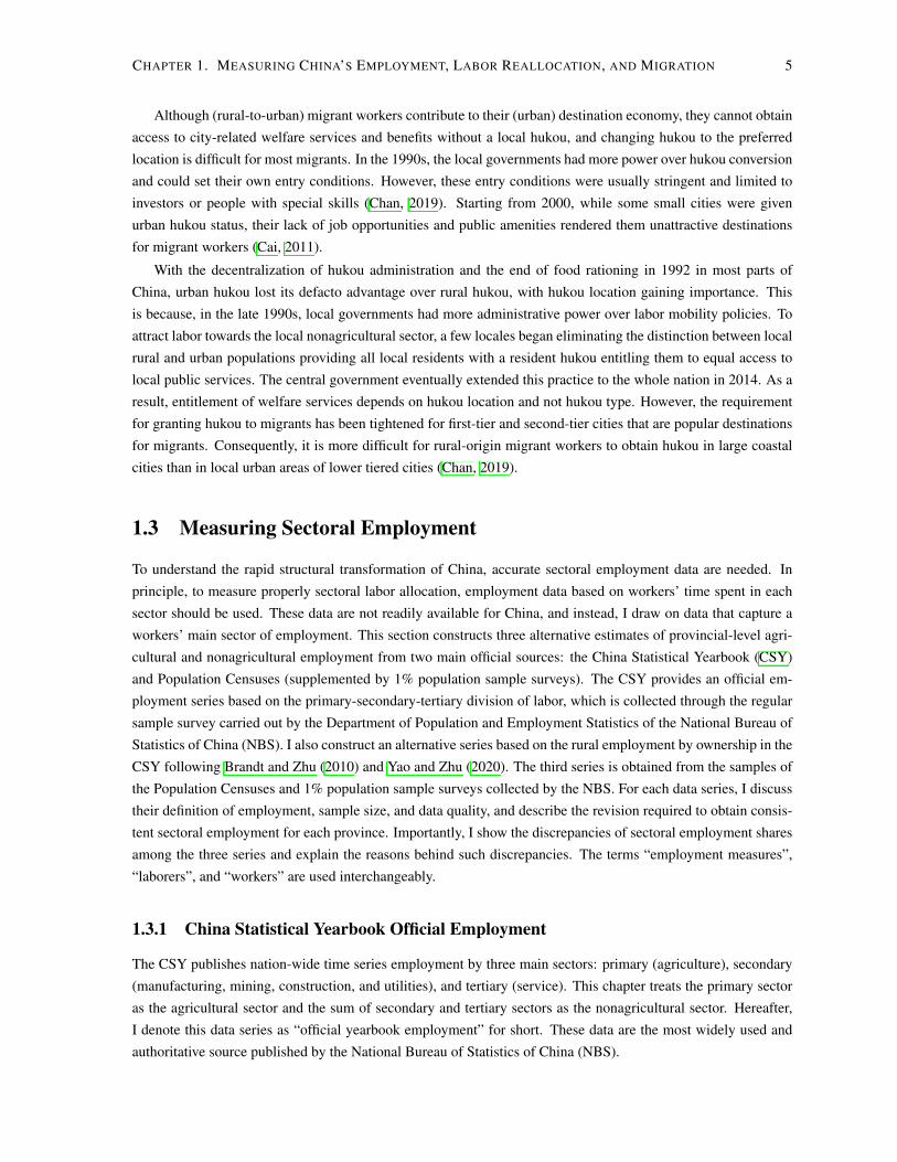
Although (rural-to-urban) migrant workers contribute to their (urban) destination economy, they cannot obtainaccess to city-related welfare services and benefits without a local hukou, and changing hukou to the preferredlocation is difficult for most migrants. In the 1990s, the local governments had more power over hukou conversionand could set their own entry conditions. However, these entry conditions were usually stringent and limited toinvestors or people with special skills (Chan, 2019). Starting from 2000, while some small cities were givenurban hukou status, their lack of job opportunities and public amenities rendered them unattractive destinationsfor migrant workers (Cai, 2011).
With the decentralization of hukou administration and the end of food rationing in 1992 in most parts ofChina, urban hukou lost its defacto advantage over rural hukou, with hukou location gaining importance. Thisis because, in the late 1990s, local governments had more administrative power over labor mobility policies. Toattract labor towards the local nonagricultural sector, a few locales began eliminating the distinction between localrural and urban populations providing all local residents with a resident hukou entitling them to equal access tolocal public services. The central government eventually extended this practice to the whole nation in 2014. As aresult, entitlement of welfare services depends on hukou location and not hukou type. However, the requirementfor granting hukou to migrants has been tightened for first-tier and second-tier cities that are popular destinationsfor migrants. Consequently, it is more difficult for rural-origin migrant workers to obtain hukou in large coastalcities than in local urban areas of lower tiered cities (Chan, 2019).
1.3 Measuring Sectoral Employment
To understand the rapid structural transformation of China, accurate sectoral employment data are needed. Inprinciple, to measure properly sectoral labor allocation, employment data based on workers’ time spent in eachsector should be used. These data are not readily available for China, and instead, I draw on data that capture aworkers’ main sector of employment. This section constructs three alternative estimates of provincial-level agri-cultural and nonagricultural employment from two main official sources: the China Statistical Yearbook (CSY)and Population Censuses (supplemented by 1% population sample surveys). The CSY provides an official em-ployment series based on the primary-secondary-tertiary division of labor, which is collected through the regularsample survey carried out by the Department of Population and Employment Statistics of the National Bureau ofStatistics of China (NBS). I also construct an alternative series based on the rural employment by ownership in theCSY following Brandt and Zhu (2010) and Yao and Zhu (2020). The third series is obtained from the samples ofthe Population Censuses and 1% population sample surveys collected by the NBS. For each data series, I discusstheir definition of employment, sample size, and data quality, and describe the revision required to obtain consis-tent sectoral employment for each province. Importantly, I show the discrepancies of sectoral employment sharesamong the three series and explain the reasons behind such discrepancies. The terms “employment measures”,“laborers”, and “workers” are used interchangeably.
1.3.1 China Statistical Yearbook Official Employment
The CSY publishes nation-wide time series employment by three main sectors: primary (agriculture), secondary(manufacturing, mining, construction, and utilities), and tertiary (service). This chapter treats the primary sectoras the agricultural sector and the sum of secondary and tertiary sectors as the nonagricultural sector. Hereafter,I denote this data series as “official yearbook employment” for short. These data are the most widely used andauthoritative source published by the National Bureau of Statistics of China (NBS).

CHAPTER 1. MEASURING CHINA’S EMPLOYMENT, LABOR REALLOCATION, AND MIGRATION 6
The CSY defines workers as persons aged 16 or above who perform a specific type of work for remuneration orbusiness income. The annual CSY reports employment by three sectors for each province. The CSY employmentdata, as originally reported in each annual yearbook, are collected via a sample survey system by the Departmentof Population and Employment Statistics of the NBS (Yue, 2005; NBS. National Bureau of Statistics of China,2016). In the remainder of this subsection, I discuss how I construct provincial-level employment data from CSYthat spans 1978 to 2015.
1.3.1.1 Official Yearbook Employment Data Construction
There are important problems at both the national and provincial level with the official employment data. Below, Idiscuss these problems and corrections made to obtain consistent province and sector level employment between1978-2015.
Figure 1.1: Employment Data in the China Statistical Yearbook
Note: This figure displays the national employment originally reported in each yearbook,NBS-revised national employment published in the 2016 yearbook, adjusted national employment,and a summation of provincial employment reported by the China Statistical Yearbook. Note thatnational employment experiences a discontinuity around 1990 and the provincial summation isconsistently lower than national employment before 2010.
First, the originally reported annual employment data published in each CSY are subject to periodical revisionby NBS. Specifically, the 1990-1995 national employment data were significantly revised upward in the 1997yearbook. Furthermore, national employment for 2001-2010 was slightly revised downward in the 2011 yearbook.Given that my period of interest spans 1978 to 2015, I therefore consult the 2016 yearbook for any updated officialnational employment figures. Figure 1.1 displays the originally reported national employment with the grey dottedline and the NBS-revised national employment from the 2016 yearbook using the red dash-dotted line.
Second, NBS only revises national employment figures starting from the year 1990. Without revision on thenational employment figures prior to 1990, there is a major discontinuity in the national employment records at1990. Following Holz (2006) and Brandt et al. (2008), I use information from the 1982 Census to make an upward

CHAPTER 1. MEASURING CHINA’S EMPLOYMENT, LABOR REALLOCATION, AND MIGRATION 7
adjustment to the pre-1990 national employment data in a way analogous to the adjustments made for 1990 andafter. This adjusted national employment is represented by the blue dashed line in Figure 1.1. I then apply theemployment shares of agriculture and nonagriculture from the official NBS data to the revised total employmentto generate the employment series for each sector before 1990. Table 1.1 displays this adjusted national-levelemployment by sector.
Third, provincial employment before 1985 and after 2010 are missing from the CSY. I supplement the missingpre-1985 and post-2010 provincial employment data using other sources. Pre-1985 provincial employment by thethree main sectors is reported in the NBS’ China Compendium of Statistics 1949-2008 (Compendium). However,these numbers should be used with caution, as the data exhibit unexplained jumps in 1990 and 1995 for someprovinces.2 Fortunately, the 1985-1990 data are consistent with the CSY and therefore I argue that the 1978-1985Compendium data can be used as a supplement.
Post-2010 provincial employment data are not reported in any NBS publications. I therefore must estimatethe 2010-2015 data from the numbers published by each province’s own statistical bureau. It is important to notethat pre-2010 provincial statistics bureau numbers are inconsistent with those of the CSY in terms of levels. Todeal with this, I only use the provincial statistics bureau’s numbers to compute annual provincial employmentgrowth rates over 2010-2015, 3 which I then apply to the 2010 CSY numbers to estimate 2011-2015 provincialemployment. This assumes that any disparity for each province is consistent for the years 2011-2015. That is tosay, if a province’s statistical bureau understates (overstates) their employment figures compared to the CSY in2010, I assume that their 2011-2015 figures are likewise understated (overstated). I then re-scale these estimated2011-2015 provincial sectoral employment numbers proportionately such that summing across the provinces ofeach sector equals the official 2011-2015 national sectoral employment reported in the CSY.
And fourth, Figure 1.1 demonstrates that the summation of CSY’s official provincial employment figures(solid black line) is consistently less than its revised national employment numbers (red dashed line post-1990).Since the NBS does not revise provincial-level employment as they do for the national employment numbers,I take provincial-level employment data as originally reported from annual CSY publications. Assuming thateach province’s employment figures are understated proportionally, I inflate provincial employment numbers over1978-2010 such that summing across provinces equals the revised total national employment of the correspondingyear. I similarly rescale each province’s agricultural employment such that the sum across provinces equalsthe national primary sector employment. The nonagricultural employment is total employment minus primaryemployment for each province and year.
1.3.2 China Statistical Yearbook Alternative Employment
There are reasons to believe that the NBS Yearbook data overestimate agriculture employment and underestimatethe rate of decline. Rawski and Mead (1998) calculates the labor requirement for agricultural production andfinds it to be smaller than the official CSY agricultural employment numbers, which means the NBS may haveoverestimated the number of agricultural workers. There are several potential reasons for this overestimation:falsely attributing those employed in private and cooperative enterprises owned by households as being part ofagriculture prior to 1984, fully counting part-time agricultural workers who may also be self-employed or workpart-time outside of agriculture, and incorrectly including migrants who left their family farm to work in the city
2For example, Jiangsu, Shandong, and Hubei provinces experience big discontinuities in 1990, 1995, and 1990, respectively. These breaksalso exist in the data published by each province’s own statistical bureau without explanation. It is very likely that the Compendium directlyadopted the numbers compiled by each provincial statistics bureau, and it may be that not all provincial statistics bureaus made adjustmentsto their data following the NBS.
3The pre-2010 growth rate of provincial statistics are similar to those in the CSY.

CHAPTER 1. MEASURING CHINA’S EMPLOYMENT, LABOR REALLOCATION, AND MIGRATION 8
(Brandt and Zhu, 2010).Brandt and Zhu (2010) study sectoral employment at the national level. They find that the official NBS agri-
cultural employment series can be closely approximated by total rural employment minus township and villageenterprise (TVEs) employment as plotted in Figure 1.2. This series, however, still leaves those employed by ruralprivate enterprises and the rural self-employed out of the nonagricultural sector. To better account for agriculturalemployment, I follow Brandt and Zhu (2010) and Yao and Zhu (2020) in constructing an alternative measure tothe official CSY agricultural employment series as follows:
Alternative Agricultural Employment =Total Rural Employment
�Township and Village Enterprise Employment
�Rural Private Enterprise Employment
�Rural Self-Employed Individuals. (1.1)
In the remainder of this subsection, I discuss the construction of this alternative yearbook employment for eachprovince in detail.
1.3.2.1 Alternative Yearbook Employment Data Construction
I construct this alternative yearbook employment measure following the methodology described in Section 1.3.1for the official yearbook employment. That is, I calculate agricultural employment at the national and provinciallevels following equation 1.1, revise or estimate the pre-1990 and post-2010 values, and then rescale the provincialemployment such that the summation of the provincial agricultural employment equals the national agriculturalemployment. The details are as follows.
First, to calculate the alternative agricultural employment at the national level, I apply equation 1.1 to thehistorical employment data published in the 2016 CSY. As can be seen in Figure 1.2, there is also a statisticalbreak in 1990 for the alternative employment measure, much like the yearbook employment data of Section1.3.1. To make the pre-1990 agricultural employment series consistent with later years, I calculate the pre-1990agricultural employment share and apply it to the revised pre-1990 total employment (refer to Section 1.3.1) toobtain my alternative agricultural employment measure. Alternative nonagricultural employment can then becalculated as the difference between the revised total employment and alternative agricultural employment.
Second, national-level TVE employment after 2010 is not reported in the CSY. An alternative source is theChina Township and Village Enterprise Yearbook (CTVEY), 4 which reports the TVE employment up to the year2013. However, the CTVEY reports a reduction in TVE employment by one-third since 2007, which deviates fromCSY numbers. This is because the CTVEY stops reporting the subcategory “other enterprises” since 2007. Toobtain a post-2010 TVE measure consistent with the CSY, I first find the 2007-2010 CTVEY “other enterprises”by CSY TVE number minus the CTVEY TVE number (without “other enterprises”). I then linearly extrapolate theCTVEY TVE (without “other enterprises”) and linearly extrapolate the “other enterprises” separately up to 2015.The summation of these two extrapolated numbers yields an estimation of TVE employment that is consistentwith the CSY.
Third, comparable data at the provincial level are only available for 1993-2010. The 1978-1993 data aresupplemented with the statistical book China Regional Economy, A profile of 17 years of reform and opening up
4China Township and Village Enterprise Yearbook is available from 1978 to 2007. In 2008 its name is changed into China Township andVillage Enterprise and Agricultural Products Processing Industries Yearbook. In 2014, the name changed again into Yearbook of China Agri-cultural Products Processing Industries following the government institutional reform that changes the name of TVE Bureau into AgriculturalProducts Processing Industries Bureau of the Ministry of Agriculture in 2013.

CHAPTER 1. MEASURING CHINA’S EMPLOYMENT, LABOR REALLOCATION, AND MIGRATION 9
Figure 1.2: Agricultural Employment
Note: This figure displays the official agricultural employment as reported by the China StatisticalYearbook, total rural employment minus rural TVE employment, and my alternative agriculturalemployment measure. All three series have a statistical break in 1990, which requires adjustment.
(17-years). However, rural private and self-employment are not reported in 17-years or any other source until1990. Before the 1978 economic reform, private and self-employment in rural areas were illegal. Therefore, I setthe 1978 starting value of these two categories to zero and linearly estimate the two series from 1978 to 1992.
Lastly, I estimate the post-2010 provincial agricultural employment data based on provincial employmentgrowth as in Section 1.3.1. Nonagricultural employment in each province is equal to total employment minusestimated agricultural employment. I then inflate provincial agricultural and nonagricultural employment propor-tionally so that the provincial summation equals the national agricultural and nonagricultural employment.
Table 1.1 documents the agricultural and nonagricultural employment given by both the CSY and my alterna-tive estimates. The latter implies a more rapid switching of labor out of agriculture. In absolute terms, nationalagricultural employment declines from 319 million in 1978 to 114 million in 2015. By 2015, my alternativeestimates suggest that the percentage of agricultural laborers fall to 15% compared to 28% in the official data.
I argue that my alternative agricultural employment series is a better measure for full-time farmers comparedto the official CSY data. For example, the 1997 Agricultural Census reports 311 million full-time farmers in1996, which is very close to the 317 million agricultural laborers in this alternative estimation compared to the348 million agricultural laborers in the official CSY data.
1.3.3 Census Employment
Since the beginning of the 1978 economic reform, China has conducted nation-wide Population Censuses for1982, 1990, 2000, 2010, and 1% population sample surveys (mini census) in the middle years. The populationcensuses and mini censuses cover a wide range of information, including employment and migration. The NBSuses the census data to update the annual CSY employment numbers.

CHAPTER 1. MEASURING CHINA’S EMPLOYMENT, LABOR REALLOCATION, AND MIGRATION 10
Table 1.1: Yearbook Employment Data (million)
TotalOfficial Employment Alternative Employment
EmploymentAg Sector Na Sector Ag Sector Na Sector
Total Percentage Total Percentage Total Percentage Total PercentageYear of total of total of total of total1978 468.43 330.36 70.52 138.07 29.48 318.74 68.04 149.69 31.961979 479.67 334.79 69.80 144.88 30.20 322.85 67.31 156.82 32.691980 493.97 339.95 68.82 154.38 31.25 330.20 66.85 163.77 33.151981 510.39 347.58 68.10 162.81 31.90 340.71 66.75 169.68 33.251982 526.18 358.48 68.13 167.70 31.87 351.00 66.71 175.18 33.291983 541.17 363.04 67.08 178.14 32.92 360.06 66.53 181.11 33.471984 558.10 357.43 64.04 200.66 35.95 345.75 61.95 212.35 38.051985 575.51 359.22 62.42 216.29 37.58 333.24 57.90 242.27 42.101986 591.51 360.51 60.95 231.00 39.05 330.79 55.92 260.72 44.081987 607.44 364.38 59.99 243.06 40.01 329.95 54.32 277.49 45.681988 622.40 369.39 59.35 253.00 40.65 330.70 53.13 291.70 46.871989 635.61 381.68 60.05 253.94 39.95 344.07 54.13 291.54 45.871990 647.49 389.14 60.10 258.35 39.90 368.39 56.90 279.10 43.101991 654.91 390.98 59.70 263.93 40.30 366.85 56.02 288.06 43.981992 661.52 386.99 58.50 274.53 41.50 358.04 54.12 303.48 45.881993 668.08 376.80 56.40 291.28 43.60 340.04 50.90 328.04 49.101994 674.55 366.28 54.30 308.27 45.70 339.18 50.28 335.37 49.721995 680.65 355.30 52.20 325.35 47.80 326.38 47.95 354.27 52.051996 689.50 348.20 50.50 341.30 49.50 316.61 45.92 372.89 54.081997 698.20 348.40 49.90 349.79 50.10 318.67 45.64 379.53 54.361998 706.37 351.77 49.80 354.60 50.20 318.92 45.15 387.45 54.851999 713.94 357.68 50.10 356.26 49.90 314.82 44.10 399.12 55.902000 720.85 360.43 50.00 360.42 50.00 320.41 44.45 400.44 55.552001 727.97 363.99 50.00 363.99 50.00 317.72 43.64 410.25 56.362002 732.80 366.40 50.00 366.40 50.00 309.48 42.23 423.32 57.772003 737.36 362.04 49.10 375.32 50.90 299.19 40.58 438.17 59.422004 742.64 348.30 46.90 394.34 53.10 290.15 39.07 452.49 60.932005 746.47 334.42 44.80 412.05 55.20 274.97 36.84 471.50 63.162006 749.78 319.41 42.60 430.37 57.40 258.89 34.53 490.89 65.472007 753.21 307.31 40.80 445.90 59.20 244.19 32.42 509.02 67.582008 755.64 299.23 39.60 456.40 60.40 230.63 30.52 525.01 69.482009 758.28 288.90 38.10 469.37 61.90 215.14 28.37 543.14 71.632010 761.05 279.31 36.70 481.74 63.30 196.38 25.80 564.67 74.202011 764.20 265.94 34.80 498.26 65.20 184.06 24.09 580.14 75.912012 767.04 257.73 33.60 509.31 66.40 168.01 21.90 599.03 78.102013 769.77 241.71 31.40 528.06 68.60 150.44 19.54 619.33 80.462014 772.53 227.90 29.50 544.63 70.50 134.43 17.40 638.10 82.602015 774.51 219.19 28.30 555.32 71.70 113.93 14.71 660.58 85.29
Note: “Ag sector” stands for agricultural sector. “Na sector” is for nonagricultural sector.

CHAPTER 1. MEASURING CHINA’S EMPLOYMENT, LABOR REALLOCATION, AND MIGRATION 11
The NBS prepares a sample of each census and mini census for research purposes. Each census sample comeswith an official sample size which is listed in the first row in Table 1.2. The census samples are random samplesof the national-wide census, which means they are representative of the population. The mini census samples aresamples of the 1% population sample surveys, meaning they are not representative of the population and weightsneed to be applied for tabulation or analysis. Fortunately, the 2005 and 2015 sample both come with officialweights prepared by the NBS. For the 2005 mini census sample, the official weight variable power 2 makes thesample tabulation by gender, province, and sector very close to the published Census Yearbook aggregate figures.
I use the 1982, 1990, 2000, 2010 census samples and the 2005, 2015 mini census samples. The census samplesrecord the occupation and industry of those aged 15 and older who have worked in the reference week before thecensus.5 To make this definition of employment comparable to that of the CSY, I limit the employment sample ofthe census and mini census to those aged 16 and above who are currently working.
Each census sample comes with an official sample size which is listed in the first row in Table 1.2. The censussamples are random samples of the national-wide census, which means they are representative of the population.The mini census samples are samples of the 1% population sample surveys, meaning they are not representative ofthe population and need to apply weights for tabulation or analysis. Fortunately, the 2005 and 2015 samples bothcome with official weights prepared by the NBS. For the 2005 mini census sample, the official weight variablepower 2 makes the sample tabulation by gender, province, and sector very close to the published census yearbook.For the 2015 mini census sample, the official weight variable qs ren is applied.
Although the official census sample generates a population number close to that reported in the CSY, thecensus employment numbers are generally smaller than those in the CSY.6 Table 1.2 row 2 (actual sample size:population) presents the census sample observation count as a fraction of the official population size as reportedin the CSY, suggesting that the samples are very close to the official sample sizes given in row 1. Row 3 (actualsample size: employment) shows that sample employment as a fraction of the CSY’s official total employment issmaller than the official sample size given in row 1. This suggests there may be undersampling of employment inthe census and mini census samples. Since this chapter focuses on employment, I inflate the census sample’s totalemployment to CSY levels, assuming this employment sample is representative.
The 1982, 1990, 2000, 2005, 2010, 2015 censuses come with industry codes. While the 1982 census followsthe pre-1984 industry classification, 1990 onwards follows the GB/T 4754 series.7 I classify the industries intoagriculture and nonagriculture.8 Table 1.2 panel B documents employment share by sector. In the period of study,agricultural employment share shrinks by half. In 2015, agricultural employment accounts for around one-thirdof total employment.
1.3.4 Discussion and Choice of Employment Data
The biggest discrepancy between CSY and census employment data lies in the agriculture and nonagriculturebreakdown. Figure 1.3 (a) presents agricultural and nonagricultural employment measures from three data series:the yearbook, alternative yearbook estimates, and census (between 1982 and 2015 when censuses are available).
5The 1982 and 1990 censuses define a worker as one who has held a fixed occupation or a temporary occupation of 16 days or more. In the2000 census and later, a worker is defined as an individual who has held a fixed occupation or worked in the week before the census. Whilethe definitions are slightly different, they are all based on current work status.
6Note that I make the census sample employment definition consistent with that of the CSY. Therefore, the employment numbers shouldbe the same.
7GB/T 4754 is the industrial classification for national economic activities published by the NBS. It was introduced in 1984 and revised in1994, 2002, and 2011, respectively. Each census follows the latest edition of the industrial classification.
8I define the agricultural sector to be consistent with that of the CSY, which excludes agriculture and agricultural service and waterconservancy. All other industries are counted as the nonagricultural sector.

CHAPTER 1. MEASURING CHINA’S EMPLOYMENT, LABOR REALLOCATION, AND MIGRATION 12
Table 1.2: Census Samples Summary
year 1982 1990 2000 2005 2010 2015Panel A: Sample SizeOfficial sample size 1% 1% 0.95% 0.20% 0.095% 0.1%(% of total number of observations)
Actual sample sizePopulation 0.99% 1.04% 0.93% 0.20% 0.095% 0.10%Employment 0.97% 1.04% 0.92% 0.19% 0.093% 0.09%
Panel B: Population and Employment (million)Adjusted Census Population and EmploymentBenchmark Population 1016.54 m 1143.33 m 1267.43 m 1307.56 m 1340.91 m 1374.62 mBenchmark Employment 526.18 m 647.49 m 720.85 m 746.47 m 761.05 m 774.51 mNa sector employment 140.82 m 186.05 m 257.03 m 308.62 m 393.17 m 490.14 mAg sector employment 385.36 m 461.44 m 463.82 m 437.85 m 367.88 m 284.37 m
Sectoral Employment SharesShare working in Na sector 26.76% 28.73% 35.66% 41.34% 51.66% 63.28%Share working in Ag sector 73.24% 71.72% 64.34% 58.66% 48.34% 36.72%
Note:1 “Ag sector” stands for agricultural sector. “Na sector” stands for nonagricultural sector.2 Given that the 2005 and 2015 mini census samples are not representative, official NBS weights power 2 and qs ren areapplied to the 2005 and 2015 mini censuses, respectively.
In general, the census data suggest a much higher level of agricultural employment than the other yearbookmeasures. In Figure 1.3 (b), we also see that the census agricultural employment share declines much slower thanthe other two measures before 2005.
The sectoral discrepancy between the census and yearbook is striking, but very few papers document thisproblem. As researchers use information from both sources, it is important to document and explain differencesbetween the two. In this subsection, I argue that the difference between the two datasets is due to part-timefarmers. I present two reasons and possible empirical evidence to support my argument. Finally, I discuss theprinciple to properly measure agricultural employment in China, which leads to future research.
First, the employment data in the census and yearbook are collected via different collection systems. Whilethe census surveys everyone9, the yearbook employment data are collected from three independent survey forms– urban working units, urban private enterprises and self-employed individuals, and rural employment. Since theyearbook surveys registered workers, it is likely that they leave informal or part-time workers out of nonagricul-tural sector. Given that agricultural production is decentralized under the HRS, farmers are most likely to be leftout from the survey.
Second, the census and yearbook are collected at different times of the year – the census surveys workersduring the busy farming season while the yearbook surveys them during the slack season. Before the year 2000,the census surveyed workers in June.10 Since the year 2000, the census has been surveying workers in late
9The 1982, 1990, 2000, and 2010 censuses survey everyone in the population while the 2005 and 2015 mini censuses survey a 1% sampleof the population.
10Before 2000, the census recorded workers’ industry and the occupation in which they worked for at least 16 days in June.

CHAPTER 1. MEASURING CHINA’S EMPLOYMENT, LABOR REALLOCATION, AND MIGRATION 13
Figure 1.3: Compare Three Sectoral Employment Measures
(a)
(b)
Note: Panel (a) ‘Ag’ stands for agricultural sector employment. ‘Na’ stands for nonagri-cultural sector employment.Panel (b) displays agricultural employment shares from three data series: census, officialyearbook and alternative yearbook.

CHAPTER 1. MEASURING CHINA’S EMPLOYMENT, LABOR REALLOCATION, AND MIGRATION 14
October.11 Since both October and June are farming seasons in China, the agricultural workers captured by thecensus includes both full-time and part-time farmers. On the other hand, the yearbook records workers’ industryat the end of the year,12 which is not a farming season. Therefore, the yearbook may not include part-time farmerswho also work in a nonagriculture job seasonally. A part-time farmer that works in the agriculture sector duringthe farming season and works in the nonagricultural sector in the non-farming season would be counted as afarmer in the census and as a worker in the yearbook.
Holz (2006) provides evidence supporting this explanation by cross-referencing the number of full-time andpart-time farmers in the 1996 Agricultural Census. He finds that the 1996 yearbook agricultural employmentfigure is close to the number of full-time farmers, which is more accurate than the census agricultural employmentfigure, which is roughly equal to full-time farmers plus individuals who are primarily but not solely in agriculture(Holz, 2006, P54, line 239).
Part-time farmers are not uncommon in developing countries undergoing structural transformation. Therefore,correctly accounting for labor input into the agricultural and nonagricultural sector is essential. In principle, toproperly account for the part-time farmers’ input into each sector, sectoral employment should be measured fromworker’s time spent in each sector. This principle is in the spirit of Rawski (1980) and Gollin et al. (2014), whichconsider labor time input in each sector instead of the total number of workers.
Brandt and Zhu (2010) estimates agricultural employment from rural household time-use data collected by theResearch Center for Rural Economy (RCRE). They find this measure to be smaller than the official yearbook’sagricultural employment figure. Brandt and Zhu (2010) suggests that the RCRE measure estimated with time-usedata is close to the alternative yearbook agricultural employment numbers. To confirm the validity of this time-use approach in measuring agricultural workers, I look into another data source – the rural sample of ChineseHousehold Income Project (CHIP) surveys – that contains the number of days rural labor spends in agricultureand nonagriculture. I first obtain an estimate of total workdays to agriculture by aggregating labor supplied tofarming by both full and part-time farmers. I do the same for labor supplied to nonagriculture for individualsworking either full or part-time in nonagriculture. I then calculate the share of total labor supplied, agricultureplus nonagriculture, that goes to agriculture. Lastly, I multiply this share by the rural labor force’s share of thetotal labor force, which gives the agriculture employment share. I plot this CHIP estimate in Figure 1.8 in theappendix. Consistent with the RCRE and alternative yearbook estimates in Brandt and Zhu (2010), this CHIPestimation also suggests fewer agricultural workers.
However, the time-use information is not available in waves earlier than 1995 of the CHIP data. Therefore,the earlier trend of farmers is unknown. The RCRE data, which surveyed household time-use between 1986 and2003 and covered all 31 provinces in China, are an alternative source of farmer time-use data. Unfortunately, thisdata is not available to the public. As a result, I adopt the official yearbook measure as a compromise. In futurework, I hope to access the RCRE data to better study sectoral labor input at the provincial level.
1.3.5 Sectoral Employment Trend by Regions
The structural transformation process did not progress evenly for all provinces. I divide the country into coastaland inland regions, as shown in Figure 1.4.13 In this subsection, I compare the sectoral employment trends
11Since 2000, the census and mini census records workers’ industry during the last week of October of the census year.12The yearbook does not document this explicitly. (Holz, 2006, line 214) explains the timing of the survey.13The coastal region is consistent with NBS’ definition of Eastern region and the inland region encompasses the NBS’ Western and Central
regions.The coastal region includes Beijing, Tianjin, Hebei, Liaoning, Shanghai, Jiangsu, Zhejiang, Fujian, Shandong, Guangdong, and HainanProvince.The inland region includes Shanxi, Inner Mongolia, Jilin, Heilongjiang, Anhui, Jiangxi, Henan, Hubei, Hunan, Guangxi, Chongqing, Sichuan,

CHAPTER 1. MEASURING CHINA’S EMPLOYMENT, LABOR REALLOCATION, AND MIGRATION 15
between the two regions using the official yearbook employment data.
Figure 1.4: Map of Coastal and Inland China
Note: This map displays the coastal region colored in red.
Figure 1.5 shows that although the coastal region accounts for only 40% of the national labor force, it has pro-portionally more workers in the nonagricultural sector since the start of the economic reform. Figure 1.6 showsthat, although the two regions experience similar rates of structural transformation (i.e. similarly sloped nona-gricultural employment share trends), the structural transformation progressed earlier in the coastal region. Thecoastal region’s nonagricultural employment share starts at 35% in 1978, which is 9 percentage points higher thanthe inland region’s 26%. This is due to higher nonagricultural employment in rural TVEs in the coastal region.At the beginning of the reform, 40% of TVE employment was located in four coastal provinces: Guangdong,Zhejiang, Shandong, and Jiangsu (BTVE, 2002, p71). The TVEs, the former rural Commune and Brigade Enter-prises, became an important driving force in nonagricultural production, giving the coastal region a head start inthe nonagricultural sector, with the inland region lagging behind for around 15 years.
This persistent gap between the inland and coastal regions is illustrated in Figure 1.6. Over the period of study,nonagricultural employment share increased by 46 percentage points and 39 percentage points in the coastal andinland regions, respectively. However, the coastal region only experienced faster structural transformation beforethe year 1990. After 1990, the share of employment in nonagriculture in the inland increases at the same rate asit does in the coastal region.
1.4 Measuring Sectoral Labor Reallocation and Migration
In this section, I use the census and mini-census samples to generate provincial-level sectoral labor reallocationand migration data. The census and mini-census samples span 1982 to 2015, capturing labor relocation since theemergence of migrant workers. Moreover, the census and mini-census samples represent a complete geographicsample of large sample size with rich details that allow me to observe individual occupation history and migration
Guizhou, Yunnan, Tibet, Shaanxi, Gansu, Qinghai, Ningxia, and Xinjiang Province.

CHAPTER 1. MEASURING CHINA’S EMPLOYMENT, LABOR REALLOCATION, AND MIGRATION 16
Figure 1.5: Employment Trends by Region
(a) (b)
Note: In panel a) and b), ‘Ag sector’ stands for nonagricultural sector and ‘Na sector’ stands for nonagricultural sector.
Figure 1.6: Nonagricultural Employment Share by Region
Note: This figure displays the nonagriculture employment share in coastal and inland region,respectively.
CHAPTER 1. MEASURING CHINA’S EMPLOYMENT, LABOR REALLOCATION, AND MIGRATION 17
trajectory at the micro-level. However, the census and mini-census samples are not perfect. Information collectedon migration behavior changes between census, making it difficult to obtain consistent worker reallocation andmigration measures. As a result, detailed estimation is needed. In this section, I explain the necessary adjustmentsto obtain long-term worker reallocation and migration from the census and present the details of my estimatedmigration measure. Moreover, I explore the possible biases of these labor reallocation and migration measures byciting numbers from other data sources.
1.4.1 Census Migration Data Construction
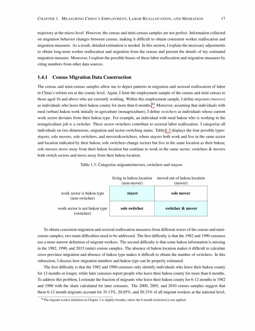
The census and mini-census samples allow me to depict patterns in migration and sectoral reallocation of laborin China’s reform era at the county level. Again, I limit the employment sample of the census and mini census tothose aged 16 and above who are currently working. Within this employment sample, I define migrants (movers)as individuals who leave their hukou county for more than 6 months.14 Moreover, assuming that individuals withrural (urban) hukou work initially in agriculture (nonagriculture), I define switchers as individuals whose currentwork sector deviates from their hukou type. For example, an individual with rural hukou who is working in thenonagriculture job is a switcher. These sector switchers contribute to sectoral labor reallocation. I categorize allindividuals on two dimensions, migration and sector-switching status. Table 1.3 displays the four possible types:stayers, sole movers, sole switchers, and movers&switchers, where stayers both work and live in the same sectorand location indicated by their hukou; sole switchers change sectors but live in the same location as their hukou;sole movers move away from their hukou location but continue to work in the same sector; switchers & moversboth switch sectors and move away from their hukou location.
Table 1.3: Categorize migrants/movers, switchers and stayers
living in hukou location moved out of hukou location(non-mover) (mover)
work sector is hukou type stayer sole mover(non-switcher)
work sector is not hukou type sole switcher switcher & mover(switcher)
To obtain consistent migration and sectoral reallocation measures from different waves of the census and mini-census samples, two main difficulties need to be addressed. The first difficulty is that the 1982 and 1990 censusesuse a more narrow definition of migrant workers. The second difficulty is that some hukou information is missingin the 1982, 1990, and 2015 (mini) census samples. The absence of hukou location makes it difficult to calculatecross-province migration and absence of hukou type makes it difficult to obtain the number of switchers. In thissubsection, I discuss how migration numbers and hukou type can be properly estimated.
The first difficulty is that the 1982 and 1990 censuses only identify individuals who leave their hukou countyfor 12 months or longer, while later censuses report people who leave their hukou county for more than 6 months.To address this problem, I estimate the fraction of migrants who leave their hukou county for 6-12 months in 1982and 1990 with the share calculated for later censuses. The 2000, 2005, and 2010 census samples suggest thatthese 6-12 month migrants account for 35.13%, 20.05%, and 20.33% of all migrant workers at the national level,
14The migrant worker definition in Chapter 3 is slightly broader, where the 6-month restriction is not applied.

CHAPTER 1. MEASURING CHINA’S EMPLOYMENT, LABOR REALLOCATION, AND MIGRATION 18
respectively. This short-term migrants share is large in the early year, declines until 2005, and remains constantafterwards. This is because when migration first surges, short-term-migrants constitute a larger proportion of allmigrants, and this fraction declines and becomes relatively constant in later years. Therefore, the proportion ofshort-term migrants may be even higher in 1982 and 1990. I linearly extend the 6-12 month national migrantsshare in 2000, 2005, and 2010 to 1982 and 1990. This extrapolation suggests that 6-12 month migrants constitute59.21% and 47.37% of total migrants in 1982 and 1990, respectively. After adding the estimated 6-12 monthmigrants, total migrants in 1982 and 1990 increase from 2.50 million and 14.61 million to 6.14 million and 27.75million, respectively.
The second difficulty is that hukou information is missing for the 1982, 1990, and 2015 censuses, respectively.In the 1990 census, 2.26% of workers are migrants who left their hukou county for more than a year, but theirhukou location is not reported. Luckily, the 1990 census reports workers’ residence five years ago, which can beused as a proxy for their hukou location. Among all 12 month+ migrants, 79.12% of them moved across countyborders within the past 5 years (recent migrants for short). These recent migrants comprise 1.79% of the laborforce. I use their previous residence to approximate their hukou location. The operating assumption here is thatmigrants move only once, which seems plausible given strict migration policies before 1990.) The remaining20.88% of the 12 months+ migrants that have been in the current county for more than 5 years (establishedmigrants for short) comprise 0.47% of the labor force. The 6-12 month migrants account for 2.03% of the laborforce, which is 47.37% of all migrants.
Laborers =
8>>>><
>>>>:
stayers and sole switchers (95.71%): origin location knownestablished migrant (0.47%): origin location unknownrecent migrant (1.79%): origin location known6-12 months migrants (2.03%): origin location unknown
For the established migrants, I estimate the proportion that move across provincial borders (established inter-province migrants) for 1990 using the known proportions for 2000. Specifically, Table 1.4 shows that, in the2000 census, 42.28% of established migrants and 61.27% of recent migrants moved between province. Giventhat established migrants are 69%(=42.28%/61.27%) less likely to move between provinces in 2000, I assumethis ratio is the same in 1990 to back out the proportion of established inter-province migrants using the knownproportion of recent inter-province migrants. The estimated inter-province fraction of established migrants is27.24%(=39.47% ⇥ 69%). The same method is applied to calculate the inter-province fraction of 6-12 monthmigrants in 1990. The inter-province share of established, recent, and 6-12 month migrants in 1990 and 2000 arepresented in Table 1.4, where shares with an asterisk are estimated from the (unasterisked) recent migrant share.I repeat this process for inter-region (coastal-inland) migrants. Aggregating these shares with the size of eachmigration category, the total number of migrants that moved inter-province and inter-region are 11.24 million and5.79 million.
The 1982 census reports only 0.48% workers left their hukou county for more than 12 months. However,neither hukou type nor hukou location is reported. To understand labor reallocation and migration, hukou typeneeds to be estimated for all workers, and hukou location needs to be estimated for migrants.
First, to obtain worker hukou type for 1982, I run a probit regression on the 1990 sample and use the coef-ficients to predict the hukou type in 1982. With the 1990 sample, I run a probit regression of the urban hukoudummy on worker characteristics, such as gender, age, education, marital status, household size, working sector,occupation, and migration status (whether moved out of hukou county for more than 12 months), as well as pre-fecture fixed effects. The model predicts an individual’s probability of having urban hukou. The aggregation of

CHAPTER 1. MEASURING CHINA’S EMPLOYMENT, LABOR REALLOCATION, AND MIGRATION 19
Table 1.4: Inter-province and Inter-region Migrant Fractions
Inter-province fraction1 Inter-region fraction2
migrant type 1990 2000 1990 2000established migrants 27.24%⇤ 42.28% 11.17%⇤ 25.63%recent migrants 39.47% 61.27% 20.50% 47.03%6-12 month migrants 44.30%⇤ 68.77% 23.41%⇤ 53.70%
Note:1 The fraction of each migrant type that moved across province borders.2 The fraction of each migrant type that crossed the coastal-inland region border.3 The shares with asterisk are estimated from the (unasterisked) migrant shares.
hukou probability at any level yields an estimate of the number of workers with urban hukou at that level.Second, I estimate the share of inter-province (inter-region) migrants. Given that an increasing number of
workers move across province (region) borders, the share of inter-province (inter-region) migrants among allmigrants increases over time. I use a simple OLS regression to extrapolate national-level inter-province (inter-region) migration share of 1990, 2000, and 2005 to 1982.15 The regression suggests that, among all 6.14 millionmigrants, 22.29% (1.37 million) migrants moved between provinces and 7.41% (0.44 million) migrants movedbetween coastal and inland regions in 1982.
The 2015 mini census does not report hukou type. Instead, individuals are asked if they have the right ofuse of their rural plot of land (land rights for short).16 While having land rights indicates agricultural hukou, lackof land rights could mean either agricultural or nonagricultural hukou, because rural households may lose theirfarmland through government expropriation and continue to hold agriculture hukou in 2015. Therefore, directlyusing land rights as hukou type would underestimate the agriculture hukou type. To estimate hukou type in 2015,I run a probit of worker hukou on worker characteristics with 2010 data and apply the coefficient on 2015 data topredict hukou types. In addition to prefecture fixed effects and area type,17 I include worker characteristics, suchas gender, age, education, marital status, working sector, occupation, and migration status. The aggregation ofhukou probability at any level yields the number of workers with urban hukou at that level.
1.4.2 Migration Trends and Patterns
This subsection describes the employment and migration patterns based on the adjusted census data. I first presentthe national employment and migration of each census year. Then, I show the inter-county and inter-provincemigration of each province. I compare the number of migrants and inter-province migrant subset across provinces.
Table 1.5 presents total employment and migrant counts for each census year. Panel A shows that the share ofemployment in nonagriculture increased by almost 40 percentage points in both the Census and Yearbook between1982 and 2015. Figure 1.7 plots the total, inter-province, and inland-coastal migration, the detailed numbers ofwhich are reported in Table 1.5 panel B. The total migrant stock, i.e. all individuals who physically move outof their hukou county, has been increasing at a greater rate over time. For example, total migrants comprise as
15The inter-province migrant share is 40.49% in 1990, 73.73% in 2000, and 76.37% in 2005. The inter-region migrant share is 20.89% in1990, 44.89% in 2000, and 47.35% in 2005.
16Chinese farmers are entitled to farmland under the current HRS system (Naughton, 2018).17The 2010 and 2015 (mini) censuses both include an area type variable that takes one of three possible values: 1=city, 2=township, or
3=village. Note that this area type classification is distinct from the administrative classification of location codes into the levels of prefecture(city), county, township, and village.

CHAPTER 1. MEASURING CHINA’S EMPLOYMENT, LABOR REALLOCATION, AND MIGRATION 20
Table 1.5: Number of Employment, Switchers and Migrants (million)
Year 1982 1990 2000 2005 2010 2015Panel A: EmploymentOfficial Yearbook employmentTotal employment 526.18 m 647.49 m 720.85 m 746.47 m 761.05 m 774.51 mNonag sector employment 167.70 m 258.35 m 360.42 m 412.05 m 481.74 m 555.32 mAg sector employment 358.48 m 389.14 m 360.43 m 334.42 m 279.31 m 219.19 mShare working in Nonag sector 31.87% 39.90% 50.00% 55.20% 63.30% 71.70%
Census employmentNonag sector employment 140.82 m 186.05 m 257.03 m 308.62 m 393.17 m 490.14 mAg sector employment 385.36 m 461.44 m 463.82 m 437.85 m 367.88 m 284.37 mShare working in Nonag sector 26.76% 28.73% 35.66% 41.34% 51.66% 63.28%
Panel B: Census MigrantsCensus Migrants: stockTotal Migrants 6.14 m 27.75 m 50.67 m 68.49 m 109.23 m 150.40 mInter-province Migrants 1.37 m 11.24 m 30.37 m 41.39 m 63.31 m 76.46 mInter-region Migrants 0.44 m 5.79 m 22.75 m 32.59 m 48.23 m 56.93 mInland-to-coastal Migrants 0.27 m 4.09 m 21.51 m 31.46 m 46.01 m 52.35 m
Census Migrants: share of employment (%)Total Migrants 1.17% 4.29% 7.03% 9.18% 14.35% 19.42%Inter-province Migrants 0.26% 1.74% 4.21% 5.54% 8.32% 9.87%Inter-region Migrants 0.08% 0.89% 3.16% 4.36% 6.34% 7.35%Inland-to-coastal Migrants 0.05% 0.63% 2.98% 4.21% 6.05% 6.76%
Panel C: Census Ag-to-Nonag SwitchersCensus Ag-to-Nonag Switchers: stockTotal Ag-to-Nonag Switchers 45.16 m 71.08 m 118.87 m 161.51 m 230.35 m 270.20 mSwitcher&Movers 2.59 m 19.08 m 36.97 m 48.78 m 79.06 m 94.48 mSwitcher&Inter-province Movers 0.58 m 7.73 m 24.26 m 33.78 m 52.48 m 59.19 mSwitcher&Inter-region Movers 0.18 m 3.65 m 18.91 m 27.58 m 41.70 m 46.56 mSwitcher&Inland-to-coastal Movers 0.10 m 2.30 m 18.10 m 26.92 m 40.34 m 43.11 m
Census Ag-to-Nonag Switchers: share of employment (%)Total Ag-to-Nonag Switchers 8.58% 10.98% 16.49% 21.64% 30.27% 34.89%Switcher&Movers 0.49% 2.95% 5.13% 6.53% 10.39% 12.20%Switcher&Inter-province Movers 0.11% 1.19% 3.37% 4.53% 6.90% 7.64%Switcher&Inter-region Movers 0.04% 0.56% 2.62% 3.69% 5.48% 6.01%Switcher&Inland-to-coastal Movers 0.02% 0.35% 2.51% 3.61% 5.30% 5.57%
Notes:1 Migrants are individuals who left their hukou county for more than 6 months. Inter-province and inter-region migrants aremigrants who crossed province and region border, respectively.2 Details of 1982, 1990, and 2015 hukou estimation see Section 1.4.1.

CHAPTER 1. MEASURING CHINA’S EMPLOYMENT, LABOR REALLOCATION, AND MIGRATION 21
Figure 1.7: Number of Migrant Workers (million)
Note: Migrant workers are individuals who left their hukou county for more than 6 months.Inter-province and inter-region migrant workers are migrant workers who crossed province andregion border, respectively.
much as 20% of total employment in 2015. Around one-third of these migrants cross region borders, the majoritymoving from inland to coastal region.
To understand how labor reallocation contributes to structural transformation, panel C presents sectoral switch-ers who hold agricultural hukou but work in nonagriculture (denoted as ag-to-nonag switchers). In 2015, theseag-to-nonag switchers account for as much as one-third of total employment. One-third of ag-to-nonag switchersmoved to another county while the remaining two-thirds remained in their hukou county. Among those ag-to-nonag switchers who moved to another county, half of them moved from inland to coastal region. The surgein rural migrant workers occurs only after 1990, suggesting that rural migrant workers were responding to therelaxation of migration policies, especially in the coastal region.
To depict these out-of-agriculture switchers and movers, I look into their characteristics. Table 1.6 shows theaverage age, female share, and years of schooling by worker’s moving/switching status for everyone who has anagricultural hukou. The movers and sole switchers are on average younger, more likely to be male, and havemore schooling. In terms of age, the movers are younger than sole switchers. The inland-to-coastal movers areeven younger than the overall movers. Meng (2012) studies the Rural Urban Migration in China and Indonesia(RUMiCI) Project data and finds that migrant workers normally go to cities in their late teens and return homearound age 30-35. The sole switchers and movers are more likely to be male than female, however, the inland-to-coastal movers are more gender-balanced. The movers and switchers received more schooling than stayers. In1990, movers, especially inland-to-coastal movers, had less schooling; however, this is no longer the case since2000, where movers have more schooling than sole switchers.
Next, I examine the migrants received by each province. Table 1.7 displays the total employment count aswell as total and inter-province migrants as a share of total employment for each province.18 The table reveals two
18The 1982 and 1990 inter-province and 2005 total migrant share are not reported due to data limitations.

CHAPTER 1. MEASURING CHINA’S EMPLOYMENT, LABOR REALLOCATION, AND MIGRATION 22
Table 1.6: Characteristics of Workers with Agricultural Hukou
Avg. Age Avg. Female Share Avg. Years of Schooling
1990 2000 2010 1990 2000 2010 1990 2000 2010Stayers 34.57 39.48 43.50 47.27% 48.63% 49.31% 5.75 6.83 7.49Sole Switchers 31.50 34.14 36.64 36.25% 34.85% 38.83% 8.15 8.30 8.97Movers 28.07 29.09 32.62 36.41% 43.57% 41.42% 7.57 8.36 9.21
Movers(Inland-to-Coastal) 24.75 26.88 31.74 48.85% 48.15% 41.97% 7.47 8.53 9.08Total 34.11 38.23 40.19 45.91% 47.08% 45.49% 6.03 7.07 8.11
Notes: This table displays average age, female labor share, and years of schooling by group for workers with agricul-tural hukou. The stayers, sole switchers and movers are mutually exclusive and the movers(inland-to-coastal) is a subsetof the movers that moved from inland to coastal region.
migration patterns. First, in the 1980s, Northeast provinces had relatively larger migrant shares of employmentcompared to other provinces. Second, since 1990, migrants became an increasingly important part of the laborforce in coastal cities and provinces, such as Beijing, Tianjin, Shanghai, and Guangdong. For example, in 2015,out-of-province workers constituted half of the labor force in Beijing and Shanghai and around one-third ofworkers in Tianjin, Zhejiang, and Guangdong.
Tables 1.8 and 1.9 present the absolute number of total and inter-province migrants received by each province.Table 1.8 examines total migration in terms of size, provincial share, and provincial rank for each province overtime. In 1982, a few eastern and central provinces (such as Heilongjiang, Henan, and Jiangsu) started to seemigrants from other counties. However, since 1990, the coastal provinces (such as Guangdong, Zhejiang, andJiangsu) became popular destinations for migrants. These three provinces, together with Shanghai, absorbed halfof China’s total migrants in 2015.
Similarly, Table 1.9 presents inter-province migration in terms of size, provincial share, and provincial rank foreach province. It further suggests that the coastal provinces accommodated most migrants from other provinces.Guangdong province has always been the most popular destination for out-of-province migrants. Guangdongencompasses three of the four original SEZs and was the recipient of much of the FDI coming in from HongKong, which was the main source of FDI for China at the beginning of the reform (Lin and Yao, 2001; Naughton,2018). Other coastal provinces (such as Jiangsu, Zhejiang, and Fujian) are likewise favored by out-of-provincemigrants.

CHAPTER 1. MEASURING CHINA’S EMPLOYMENT, LABOR REALLOCATION, AND MIGRATION 23
Tabl
e1.
7:Em
ploy
men
tand
Inte
r-C
ount
y,In
ter-
Prov
ince
Mig
ratio
nby
Prov
ince
1982
1990
2000
2005
2010
2015
Inte
rIn
ter
Inte
rIn
ter
Inte
rIn
ter
Inte
rIn
ter
Inte
rPr
ovin
ceEm
p.C
ty.
Emp.
Cty
.Em
p.C
ty.
Prov
.Em
p.C
ty.
Prov
.Em
p.C
ty.
Prov
.Em
p.Pr
ov.
(%)
(%)
(%)
(%)
(%)
(%)
(%)
(%)
(%)
Nat
iona
l52
6.18
m1.
1764
7.49
m4.
2972
0.85
m7.
034.
2174
6.47
m9.
185.
5476
1.05
m14
.35
8.32
774.
51m
9.87
Bei
jing
5.56
m1.
406.
17m
9.54
7.43
m24
.10
23.0
78.
00m
38.2
831
.00
10.3
5m
54.1
945
.18
11.8
8m
47.7
6Ti
anjin
4.55
m1.
926.
29m
14.8
64.
98m
8.52
7.97
5.67
m18
.52
15.6
95.
77m
28.0
121
.79
8.67
m35
.93
Heb
ei28
.01
m1.
2031
.82
m2.
5240
.92
m2.
781.
3341
.46
m2.
921.
1343
.21
m4.
691.
8941
.61
m2.
60Sh
anxi
13.2
5m
1.19
14.7
9m
4.22
17.3
4m
3.83
1.91
17.1
6m
3.71
1.41
18.3
1m
8.62
2.89
18.5
5m
2.80
Inne
rMon
golia
9.14
m2.
3112
.80
m6.
1113
.43
m6.
982.
2914
.01
m9.
373.
3713
.53
m17
.80
5.90
13.6
8m
5.94
Liao
ning
18.0
7m
0.96
23.2
1m
3.99
23.5
0m
5.11
2.39
23.2
3m
8.18
3.03
24.9
5m
11.9
34.
3224
.05
m3.
73Ji
lin9.
69m
2.10
13.5
1m
3.38
14.1
2m
3.22
1.13
13.9
9m
4.35
1.20
14.9
6m
6.90
1.65
15.5
5m
1.52
Hei
long
jiang
13.4
1m
4.00
18.2
7m
7.00
18.2
2m
5.20
1.18
19.6
2m
4.94
0.98
20.0
3m
6.71
1.13
20.2
0m
1.06
Shan
ghai
7.63
m1.
729.
66m
17.1
48.
79m
30.1
524
.00
9.68
m45
.45
38.2
513
.27
m61
.31
53.7
814
.35
m56
.20
Jian
gsu
35.1
7m
1.11
41.2
7m
3.83
45.6
0m
7.37
3.90
46.1
2m
13.8
57.
8347
.67
m20
.10
12.2
349
.33
m14
.66
Zhej
iang
21.1
3m
1.02
24.8
1m
5.43
28.1
1m
13.7
29.
6129
.29
m22
.29
18.3
135
.11
m35
.22
29.1
434
.01
m29
.16
Anh
ui26
.00
m1.
3638
.71
m3.
5834
.96
m1.
880.
4138
.33
m3.
070.
6030
.39
m6.
111.
2435
.14
m2.
97Fu
jian
11.7
5m
1.83
16.1
4m
7.54
17.9
9m
13.1
47.
7319
.47
m21
.34
12.9
920
.50
m25
.58
15.3
621
.38
m16
.66
Jian
gxi
15.6
6m
0.98
22.8
3m
2.79
19.8
6m
2.43
0.64
21.9
6m
2.45
0.67
23.7
4m
3.88
1.08
24.4
0m
1.82
Shan
dong
40.5
5m
0.91
47.8
5m
2.07
58.4
7m
2.92
1.14
58.8
5m
4.35
1.53
60.8
1m
5.89
1.81
60.7
5m
2.11
Hen
an40
.26
m1.
3348
.76
m2.
3957
.37
m1.
630.
4255
.31
m1.
590.
3053
.88
m4.
080.
5748
.82
m1.
53H
ubei
25.9
2m
1.30
31.5
7m
3.50
30.6
6m
4.00
1.11
32.8
9m
4.28
0.88
31.7
0m
7.88
1.54
32.1
7m
3.56
Hun
an28
.52
m0.
5534
.49
m1.
7835
.25
m2.
410.
4935
.81
m3.
560.
6236
.51
m4.
930.
8937
.18
m2.
37G
uang
dong
28.2
4m
0.92
31.9
5m
13.4
048
.06
m35
.40
27.0
355
.31
m36
.62
28.2
959
.07
m42
.98
31.8
166
.08
m32
.63
Gua
ngxi
18.7
2m
0.74
23.3
8m
2.67
25.6
5m
3.67
0.85
25.4
8m
3.84
0.90
26.2
8m
7.91
2.04
26.0
0m
3.07
Hai
nan
2.83
m2.
343.
49m
11.6
43.
99m
8.27
5.08
4.54
m8.
333.
934.
32m
14.4
76.
514.
80m
9.37
Cho
ngqi
ng15
.23
m0.
1817
.63
m1.
8417
.12
m3.
011.
3816
.36
m3.
681.
3714
.61
m10
.92
3.82
16.2
5m
5.22
Sich
uan
39.8
3m
0.31
46.6
4m
2.26
49.2
7m
2.92
0.54
48.6
7m
3.30
0.68
49.8
8m
7.88
1.29
47.2
7m
2.41
Gui
zhou
13.9
8m
0.76
16.5
0m
1.74
20.3
4m
3.28
1.16
20.4
3m
3.63
1.24
17.9
8m
7.81
2.54
17.0
8m
4.62
Yunn
an16
.61
m0.
5920
.22
m3.
3326
.47
m5.
692.
7828
.34
m5.
241.
9728
.17
m7.
762.
8229
.30
m3.
64Ti
bet
1.02
m0.
001.
18m
1.47
1.43
m6.
354.
811.
70m
2.63
1.76
1.53
m11
.06
8.61
2.17
m7.
16Sh
aanx
i15
.22
m1.
2517
.71
m4.
1619
.92
m2.
721.
0321
.68
m3.
361.
1421
.11
m7.
332.
3319
.46
m2.
80G
ansu
10.3
6m
0.85
13.5
7m
2.07
15.0
8m
2.42
0.87
15.4
9m
2.00
0.64
14.7
8m
5.16
1.51
14.6
3m
2.16
Qin
ghai
1.86
m2.
282.
98m
6.77
2.80
m5.
592.
412.
97m
6.25
2.77
3.04
m16
.48
7.75
3.15
m9.
15N
ingx
ia1.
80m
1.03
1.90
m1.
253.
16m
6.48
3.40
3.43
m5.
132.
093.
34m
15.6
96.
883.
55m
6.49
Xin
jiang
6.19
m5.
407.
42m
10.1
010
.55
m11
.84
9.50
11.2
2m
8.35
5.87
12.2
4m
14.2
79.
0713
.05
m10
.70
1“E
mp.
”is
num
bero
fem
ploy
men
t.“I
nter
-Cty
.(%)”
isin
ter-
coun
tym
igra
nts
asa
shar
eof
empl
oym
ent.
“Int
er-P
rov.
(%)”
isin
ter-
prov
ince
mig
rant
sas
ash
are
ofem
ploy
men
t.2
The
1982
and
1990
mig
rant
sar
ees
timat
edw
ithtim
e-m
ultip
liert
hati
nclu
des
6-12
mon
ths
mig
rant
s.D
etai
lsse
eSe
ctio
n1.
4.1.
3H
aina
npr
ovin
cew
aspa
rtof
Gua
ngdo
ngpr
ovin
cebe
fore
1988
and
Cho
ngqi
ngm
unic
ipal
ityw
aspa
rtof
Sich
uan
prov
ince
befo
re19
97.I
n19
82an
d19
90ce
nsus
,Itre
atth
epr
efec
ture
sla
terb
elon
gto
Hai
nan
and
Cho
ngqi
ngas
thes
etw
opr
ovin
ces.

CHAPTER 1. MEASURING CHINA’S EMPLOYMENT, LABOR REALLOCATION, AND MIGRATION 24
Tabl
e1.
8:In
ter-
Cou
nty
Mig
ratio
nSi
zean
dPr
ovin
cial
Shar
e
1982
1990
2000
2005
2010
Prov
.Pr
ov.
Prov
.Pr
ov.
Prov
.Pr
ov.
Prov
.Pr
ov.
Prov
.Pr
ov.
Prov
ince
Mig
.Sh
are
Ran
kM
ig.
Shar
eR
ank
Mig
.Sh
are
Ran
kM
ig.
Shar
eR
ank
Mig
.Sh
are
Ran
k(%
)(%
)(%
)(%
)(%
)N
atio
nal
6.14
m10
027
.75
m10
050
.67
m10
068
.49
m10
010
9.23
m10
0B
eijin
g0.
08m
1.27
260.
59m
2.12
231.
79m
3.53
63.
06m
4.47
65.
61m
5.13
5Ti
anjin
0.09
m1.
4225
0.93
m3.
3712
0.42
m0.
8426
1.05
m1.
5316
1.62
m1.
4819
Heb
ei0.
34m
5.49
60.
80m
2.89
141.
14m
2.25
131.
21m
1.77
142.
03m
1.86
15Sh
anxi
0.16
m2.
5716
0.62
m2.
2521
0.66
m1.
3120
0.64
m0.
9323
1.58
m1.
4521
Inne
rMon
golia
0.21
m3.
4512
0.78
m2.
8215
0.94
m1.
8516
1.31
m1.
9212
2.41
m2.
2011
Liao
ning
0.17
m2.
8315
0.93
m3.
3413
1.20
m2.
3712
1.90
m2.
788
2.98
m2.
739
Jilin
0.20
m3.
3113
0.46
m1.
6524
0.46
m0.
9025
0.61
m0.
8924
1.03
m0.
9425
Hei
long
jiang
0.54
m8.
741
1.28
m4.
616
0.95
m1.
8714
0.97
m1.
4118
1.34
m1.
2324
Shan
ghai
0.13
m2.
1420
1.66
m5.
972
2.65
m5.
234
4.40
m6.
424
8.14
m7.
454
Jian
gsu
0.39
m6.
343
1.58
m5.
693
3.36
m6.
633
6.39
m9.
323
9.58
m8.
773
Zhej
iang
0.22
m3.
5010
1.35
m4.
855
3.86
m7.
612
6.53
m9.
532
12.3
7m
11.3
22
Anh
ui0.
35m
5.77
51.
39m
4.99
40.
66m
1.30
211.
18m
1.72
151.
86m
1.70
16Fu
jian
0.21
m3.
5011
1.22
m4.
397
2.36
m4.
665
4.16
m6.
075
5.24
m4.
806
Jian
gxi
0.15
m2.
4918
0.64
m2.
3019
0.48
m0.
9524
0.54
m0.
7926
0.92
m0.
8426
Shan
dong
0.37
m6.
044
0.99
m3.
5611
1.71
m3.
377
2.56
m3.
747
3.58
m3.
288
Hen
an0.
53m
8.71
21.
17m
4.21
80.
94m
1.85
170.
88m
1.28
202.
20m
2.01
12H
ubei
0.34
m5.
487
1.11
m3.
989
1.23
m2.
4211
1.41
m2.
0611
2.50
m2.
2910
Hun
an0.
16m
2.57
160.
61m
2.21
220.
85m
1.68
181.
27m
1.86
131.
80m
1.65
17G
uang
dong
0.26
m4.
269
4.28
m15
.42
117
.02
m33
.58
120
.25
m29
.57
125
.39
m23
.24
1G
uang
xi0.
14m
2.26
190.
62m
2.25
200.
94m
1.86
150.
98m
1.43
172.
08m
1.90
14H
aina
n0.
07m
1.08
270.
41m
1.46
250.
33m
0.65
280.
38m
0.55
270.
63m
0.57
28C
hong
qing
0.03
m0.
4529
0.32
m1.
1726
0.52
m1.
0223
0.60
m0.
8825
1.60
m1.
4620
Sich
uan
0.12
m2.
0321
1.06
m3.
8010
1.44
m2.
849
1.61
m2.
359
3.93
m3.
607
Gui
zhou
0.11
m1.
7322
0.29
m1.
0427
0.67
m1.
3219
0.74
m1.
0821
1.40
m1.
2923
Yunn
an0.
10m
1.59
230.
67m
2.43
181.
51m
2.97
81.
49m
2.17
102.
19m
2.00
13Ti
bet
0.00
m0.
0031
0.02
m0.
0631
0.09
m0.
1831
0.04
m0.
0731
0.17
m0.
1531
Shaa
nxi
0.19
m3.
1114
0.74
m2.
6617
0.54
m1.
0722
0.73
m1.
0622
1.55
m1.
4222
Gan
su0.
09m
1.43
240.
28m
1.01
280.
36m
0.72
270.
31m
0.45
280.
76m
0.70
27Q
ingh
ai0.
04m
0.69
280.
20m
0.73
290.
16m
0.31
300.
19m
0.27
290.
50m
0.46
30N
ingx
ia0.
02m
0.30
300.
02m
0.09
300.
20m
0.40
290.
18m
0.26
300.
52m
0.48
29X
injia
ng0.
33m
5.45
80.
75m
2.70
161.
25m
2.47
100.
94m
1.37
191.
75m
1.60
181
“Mig
.”is
num
bero
fint
er-c
ount
ym
igra
nt.“
Prov
Shar
e.(%
)”is
prov
inci
alin
ter-
coun
tym
igra
nts
asa
shar
eof
tota
lint
er-c
ount
ym
igra
nts.
2Th
e19
82an
d19
90m
igra
nts
are
estim
ated
with
time-
mul
tiplie
rtha
tinc
lude
s6-
12m
onth
sm
igra
nts.
Det
ails
see
Sect
ion
1.4.
1.3
Hai
nan
prov
ince
was
part
ofG
uang
dong
prov
ince
befo
re19
88an
dC
hong
qing
city
was
part
ofSi
chua
npr
ovin
cebe
fore
1997
.In
the
1982
and
1990
cens
us,I
treat
the
pref
ectu
res
late
rbe
long
toH
aina
nan
dC
hong
qing
asth
ese
two
prov
ince
s.

CHAPTER 1. MEASURING CHINA’S EMPLOYMENT, LABOR REALLOCATION, AND MIGRATION 25
Tabl
e1.
9:In
ter-
Prov
ince
Mig
ratio
nSi
zean
dPr
ovin
cial
Shar
e
1990
2000
2005
2010
2015
Prov
.Pr
ov.
Prov
.Pr
ov.
Prov
.Pr
ov.
Prov
.Pr
ov.
Prov
.Pr
ov.
Prov
ince
Mig
.Sh
are
Ran
kM
ig.
Shar
eR
ank
Mig
.Sh
are
Ran
kM
ig.
Shar
eR
ank
Mig
.Sh
are
Ran
k(%
)(%
)(%
)(%
)(%
)N
atio
nal
100.
030
.37
m10
041
.39
m10
063
.31
m10
076
.46
m10
0B
eijin
g5.
254
1.71
m5.
645
2.48
m6.
006
4.68
m7.
385
5.67
m7.
425
Tian
jin6.
963
0.40
m1.
3112
0.89
m2.
158
1.26
m1.
987
3.11
m4.
077
Heb
ei2.
6216
0.55
m1.
8011
0.47
m1.
1313
0.81
m1.
2911
1.08
m1.
4212
Shan
xi3.
579
0.33
m1.
0914
0.24
m0.
5818
0.53
m0.
8417
0.52
m0.
6823
Inne
rMon
golia
2.83
140.
31m
1.01
150.
47m
1.14
120.
80m
1.26
120.
81m
1.06
18Li
aoni
ng3.
4710
0.56
m1.
8510
0.70
m1.
709
1.08
m1.
7010
0.90
m1.
1715
Jilin
1.29
220.
16m
0.52
250.
17m
0.41
250.
25m
0.39
260.
24m
0.31
28H
eilo
ngjia
ng4.
107
0.21
m0.
7121
0.19
m0.
4623
0.23
m0.
3629
0.21
m0.
2830
Shan
ghai
11.3
42
2.11
m6.
953
3.70
m8.
953
7.14
m11
.28
38.
06m
10.5
53
Jian
gsu
5.16
51.
78m
5.86
43.
61m
8.73
45.
83m
9.21
47.
23m
9.46
4Zh
ejia
ng1.
8420
2.70
m8.
902
5.36
m12
.95
210
.23
m16
.16
29.
92m
12.9
72
Anh
ui2.
2218
0.14
m0.
4726
0.23
m0.
5519
0.38
m0.
5921
1.04
m1.
3714
Fujia
n3.
0412
1.39
m4.
586
2.53
m6.
115
3.15
m4.
976
3.56
m4.
666
Jian
gxi
2.54
170.
13m
0.42
280.
15m
0.35
270.
26m
0.40
250.
44m
0.58
25Sh
ando
ng3.
1611
0.66
m2.
199
0.90
m2.
187
1.10
m1.
749
1.28
m1.
689
Hen
an2.
6415
0.24
m0.
7917
0.17
m0.
4026
0.31
m0.
4923
0.75
m0.
9821
Hub
ei3.
578
0.34
m1.
1213
0.29
m0.
7015
0.49
m0.
7719
1.14
m1.
5010
Hun
an0.
8727
0.17
m0.
5724
0.22
m0.
5322
0.33
m0.
5222
0.88
m1.
1516
Gua
ngdo
ng16
.31
112
.99
m42
.78
115
.65
m37
.81
118
.79
m29
.68
121
.57
m28
.20
1G
uang
xi1.
1224
0.22
m0.
7220
0.23
m0.
5520
0.54
m0.
8516
0.80
m1.
0419
Hai
nan
1.76
210.
20m
0.67
230.
18m
0.43
240.
28m
0.44
240.
45m
0.59
24C
hong
qing
0.49
290.
24m
0.78
180.
22m
0.54
210.
56m
0.88
150.
85m
1.11
17Si
chua
n0.
9525
0.26
m0.
8716
0.33
m0.
8014
0.64
m1.
0214
1.14
m1.
4911
Gui
zhou
1.26
230.
24m
0.78
190.
25m
0.61
160.
46m
0.72
200.
79m
1.03
20Yu
nnan
3.03
130.
74m
2.43
80.
56m
1.35
110.
79m
1.25
131.
07m
1.39
13Ti
bet
0.00
310.
07m
0.23
300.
03m
0.07
310.
13m
0.21
310.
16m
0.20
31Sh
aanx
i2.
1419
0.21
m0.
6822
0.25
m0.
6017
0.49
m0.
7818
0.54
m0.
7122
Gan
su0.
5528
0.13
m0.
4327
0.10
m0.
2428
0.22
m0.
3530
0.32
m0.
4126
Qin
ghai
0.91
260.
07m
0.22
310.
08m
0.20
290.
24m
0.37
270.
29m
0.38
27N
ingx
ia0.
1330
0.11
m0.
3529
0.07
m0.
1730
0.23
m0.
3628
0.23
m0.
3029
Xin
jiang
4.88
61.
00m
3.30
70.
66m
1.59
101.
11m
1.75
81.
40m
1.83
81
“Mig
.”is
num
bero
fint
er-c
ount
ym
igra
nt.“
Prov
Shar
e.(%
)”is
inte
r-pr
ovin
cem
igra
tion
asa
shar
eof
tota
lint
er-p
rovi
nce
mig
ratio
nfo
reac
hpr
ovin
ce.

CHAPTER 1. MEASURING CHINA’S EMPLOYMENT, LABOR REALLOCATION, AND MIGRATION 26
1.4.3 Discussion on Sectoral Labor Reallocation and Migration Measures
In this subsection, I discuss the possible biases of the census labor reallocation and migration measures by citingnumbers from other data sources. I first compare the number of migrant workers to the migrant population that iswidely cited in the literature. I then discuss the role of part-time farmers found in Section 1.3.4. Lastly, I discussthe possible bias of using hukou type and location as one’s origin and find the potential bias in this measure.
1.4.3.1 Migrant Population and Migrant Workers
Following each census, the CSY reports the migrant population stock who left their hukou for more than 6months,19 which is widely cited in the literature. I present this CSY migrant population alongside my revisedmigrant worker series in Table 1.10. Column A is the total migrant population who left their hukou township(inter-township) for more than 6 months, which I take directly from the CSY. In column B, I document the inter-county migrant population from various census tabulations published by the NBS.20 Among the migrants whomoved between townships (column A) in 2000, 55% (78.8/144.4) moved between counties for job opportunities(column C). This percentage increases to 72% in 2015, suggesting an increasing number of people moving furtheraway from home to find work.
Columns C and D present the stock of migrant workers under different geographical definitions from myadjusted migrant worker series. Columns C and D’s migrant workers are subsets of the migrant population incolumns A and B, respectively. In general, around 60% of the migrant population are workers, which is slightlyhigher than the average labor-population ratio of 56%. For example, in 2000, out of the 144 million who hadmoved townships, 85 million were workers; and in 2010, out of the 261 million who had moved townships, 153million were workers.
Column E and F further report rural-to-urban migrant workers – workers with agricultural hukou who work inthe nonagricultural sector (ag-to-nonag). Assuming that individuals with rural hukou work initially in agriculture,column E and F capture rural migrant workers who switch to nonagriculture and contribute to structural transfor-mation. 21 Comparing column F to D, rural migrant workers comprise as much as three-quarters of migrants.
1.4.3.2 Part-time Farmers
Section 1.3.4 concludes that agricultural employment difference between the CSY and census is possibly dueto part-time farmers. It is difficult to decide how to treat part-time farmers without more information. But thecensus’ higher agricultural employment may lead to an underestimation of the number of ag-to-nonag switchers.If the CSY-census agricultural employment gap is comprised entirely of part-time farmers who spend most oftheir time in local nonagricultural jobs, this gap should be counted towards ag-to-nonag sole switchers. Thenumber of part-time farmers grew from as low as 27 million in 1982 to 103 million in 2005 before it dropped to65 million in 2015. This extreme scenario rendered the number of ag-to-nonag switchers to be much larger than
19The CSY not only report migrant population in the census years, but also estimates the number of migrants for non-census years.20They are Tabulation on the 1995 1% Population Sample Survey, Table 7-1, 7-3.
Tabulation on the 2000 Population Census of PRC, Table 7-1,Tabulation on the 2010 Population Census of PRC, Table 1-4,Tabulation on the 2015 1% Population Sample Survey, Table 12-9.
21An alternative rural migrant worker measure is the Migrant Workers Monitoring Survey (MWMS) Report. The NBS initiated this surveyin 2008 and report the aggregated number of rural migrants annually. This survey targets the same group as my estimates in column E (i.e.workers who have hukou in villages and work in the nonagricultural sector in another township for at least 6 months) but the MWMS revealsmuch more rural migrant workers. For example, the MWMS reports 153 million rural migrant workers in 2010, which is significantly largerthan 95.9 million in my estimates reported in column E. No literature or official document explains the discrepancy between the two sources,which consequently remains a puzzle.

CHAPTER 1. MEASURING CHINA’S EMPLOYMENT, LABOR REALLOCATION, AND MIGRATION 27
Table 1.10: Major Aggregated Migration Statistics (million)
Census Migrant Population Census Migrant Worker1
Boundary Township County Township County Township CountyWorker Type All All All All Ag-to-Nonag Ag-to-Nonag
Year A B C D E F1982 6.14 2.591990 27.75 19.081995 49.7 29.12000 144.4 78.8 85.2 50.67 45.9 36.972005 153.1 94.9 97.8 68.49 58.3 48.782010 261 166 152.6 109.23 95.9 79.062011 2712012 2792013 2892014 2982015 294 212 150.4 94.482016 2922017 2912018 286
Note:1 All migrants left their hukou county for more than 6 months.2 “Ag hukou” stands for agricultural hukou. “Nonag hukou” is for nonagricultural hukou.Column A: 2019 China Statistical Yearbook, Table 2-3 “population left hukou township”.Column B source:
Tabulation on the 1995 1% Population Sample Survey, Table 7-1, 7-3.Tabulation on the 2000 Population Census of PRC, Table 7-1.1982, 2005 (mini) census sample - estimated by author.Tabulation on the 2010 Population Census of PRC, Table 1-4.Tabulation on the 2015 1% Population Sample Survey, Table 12-9.
Column C, D, E, and F: Tabulation on census samples - estimated by author.

CHAPTER 1. MEASURING CHINA’S EMPLOYMENT, LABOR REALLOCATION, AND MIGRATION 28
that documented in Table 1.5. To estimate the upper bound for ag-to-nonag switchers, I take this CSY-censusagricultural employment gap as the number of additional ag-to-nonag switchers. Table 1.11 panel A suggests thatincluding part-time farmers significantly increases the number of ag-to-nonag switchers. This new measure is aslarge as 2 times that of the census measure of ag-to-nonag switchers for 1990; and declines to 1.24 times of thecensus measure for 2015. While these additional sole switchers do not affect the measure of migrants, they drivedown the percentage of migrants’ contribution to structural change.
Table 1.11: Ag-to-Nonag Switchers and Switcher&Movers (million)
Panel A: Ag-to-Nonag SwitchersYear Employment Census Measure Including Part-time Farmers1 Including Hukou Changers2
Total Percentage Total Percentage Total Percentageof employment of employment of employment
1982 526.18 m 45.16 m 8.58% 72.04 m 13.69% 45.16 m 8.58%1990 647.49 m 71.08 m 10.98% 139.96 m 21.62% 84.81 m 13.10%2000 720.85 m 118.87 m 16.49% 222.26 m 30.83% 146.91 m 20.38%2005 746.47 m 161.51 m 21.64% 264.94 m 35.49% 197.41 m 26.45%2010 761.05 m 230.35 m 30.27% 318.92 m 41.91% 276.70 m 36.36%2015 774.51 m 270.20 m 34.89% 335.38 m 43.30% - -
Panel B: Ag-to-Nonag Switcher&MoversYear Employment Census Measure Including Part-time Farmers Including Hukou Changers
Total Percentage Total Percentageof employment of employment
1982 526.18 m 2.59 m 0.49% 2.59 m 0.49%1990 647.49 m 19.08 m 2.95% 32.81 m 5.07%2000 720.85 m 36.97 m 5.13% 65.01 m 9.02%2005 746.47 m 48.78 m 6.53% 84.69 m 11.34%2010 761.05 m 79.06 m 10.39% 125.41 m 16.48%2015 774.51 m 94.48 m 12.20% - -
Note:1 These columns treat part-time farmers as sole ag-to-nonag switchers. The number of part-time farmers is the differencebetween yearbook and census agricultural employment.2 These columns treat hukou changers as ag-to-nonag switchers and ag-to-nonag switcher&movers. The number ofhukou changers is estimated from the Chinese Household Income Project (CHIP) surveys.
1.4.3.3 Changing Hukou
To identify the number of migrants, I assume that individuals do not change their hukou location and type. Thisis potentially violated if individuals successfully change their hukou location and type. Using hukou location asone’s origin would miss out on these hukou-changing migrants, and I would therefore underestimate the totalnumber of migrants. To quantify this bias, I estimate the number of permanent migrants with information fromother general surveys. 22 The Chinese Household Income Project (CHIP) 1999, 2002, 2007, 2008, 2013 urbansamples ask people whether they changed their hukou type. However, changing hukou location is a subset ofchanging hukou type, because rural residents may also be granted urban hukou through land expropriation or land
22Many survey datasets have migration-related questions in selected waves. However, most migration questions only appear after the year2000, which does not allow for analysis in the early reform period. To be more specific, the Chinese Household Income Project (CHIP) surveystarts as early as 1988 but 1999 is the earliest wave that includes migration-related questions. Rural-Urban Migration in China (RUMIC)focuses on migration but begins in 2008. Other surveys, such as the Chinese General Social Survey (CGSS), China Family Panel Studies(CFPS), and China Labor-force Dynamics Survey (CLDS) start in 2003, 2010, and 2012, respectively.

CHAPTER 1. MEASURING CHINA’S EMPLOYMENT, LABOR REALLOCATION, AND MIGRATION 29
reclassification without moving. Therefore, using this CHIP measure of hukou type changers serves as an upperbound for the number of migrants who change their hukou location. Table 1.12 panel A documents the fraction ofurban hukou workers who changed their hukou type from rural to urban. Panel B presents the linear extrapolationof this fraction across census years. I then apply this predicted fraction to the number of urban hukou holdersfound in the census and report the number of estimated hukou changers in Panel B. The number of hukou typechangers can be as much as 14 million in 1990 and grows to as much as 46 million in 2010, where the latteraccounts for 6% of the labor force.
Table 1.12: Fraction of Hukou Changers among Urban Nonagricultural Workers
Panel A: Fraction of Hukou Changers (CHIP Urban Sample)1
Year 1999 2002 2007 2008 2013Fraction 15.80% 23.08% 26.14% 24.21% 28.26%
Panel B: Predicted Fraction of Hukou ChangersYear 1990 2000 2005 2010 2015Predicted Fraction 11.13% 18.96% 22.87% 26.78% 30.70%
Predicted Hukou Changers 14.27 m 27.83 m 35.88 m 46.35 m -
Note: Chinese Household Income Project (CHIP) urban samples only identify people whochanged hukou type from rural to urban without asking their migration experience. Therefore,the CHIP data give an upper bound of the ideal hukou changer measure.
Table 1.11 panel A reports ag-to-nonag switchers including hukou changers. Panel B reports the subcategoryag-to-nonag switcher&movers including hukou changers. Since changing hukou type and location was strictlyrestricted by the government at the beginning of the reform, I assume the number of hukou changers is zero in1982. When accounting for hukou changers, ag-to-nonag switchers (in panel A) increase by 20% and ag-to-nonagswitcher&movers (in panel B) increase by 58% in 2010.
1.5 Contribution of Switchers and Movers to Structural Transformation
Between 1978 and 2015, the total labor force increased by 47%, which led to an increase in nonagriculturalemployment. Besides this natural population growth, workers switching from agriculture to nonagriculture con-stituted an important force that accelerated structural transformation. This section links sectoral switchers as wellas its subcategory switcher&movers to structural transformation. Table 1.13 subpanel 1 first presents nonagricul-tural employment from the official CSY employment series, the number of sectoral switchers from agricultureto nonagriculture (ag-to-nonag switchers), and the subset of switchers who are also movers, as documented inTable 1.5. I then calculate the five-year increment of these three groups which is documented in subpanel 2.Specifically, I linearly interpolate year 1985 and 1995 figures for the years 1990 and 2000 to calculate five-yearincrements.23 To understand how ag-to-nonag switchers’ growth contributes to nonagricultural sectoral growth,let us look at subpanel 2, entitled Employment and Switcher 5-year Increment. In this subpanel, I compare thefive-year increment of ag-to-nonag switchers (row 2) to that of nonagricultural employment (row 1). Additionally,I compare the five-year increment of individuals who are both ag-to-nonag switcher&movers (row 3) to that ofnonagricultural employment (row 1). Subpanel 2 suggests that nonagricultural employment increases at a constant
23All figures for the years 1990 and 2000 are estimated as linearly interpolated midpoints. The 1990 values are calculated as x1990 �x1985 =x1990 � ( 5
8 x1982 +38 x1990). The 2000 values are x2000 � x1995 = x2000 � ( 1
2 x1990 +12 x2000).

CHAPTER 1. MEASURING CHINA’S EMPLOYMENT, LABOR REALLOCATION, AND MIGRATION 30
Table 1.13: Contribution of Switchers and Movers to Structural Transformation (National)
Panel 1: Employment and Switcher LevelYear 1982 1990 2000 2005 2010 2015Total Employment 526.18 m 647.49 m 720.85 m 746.47 m 761.05 m 774.51 mNonag Sector Employment 167.70 m 258.35 m 360.42 m 412.05 m 481.74 m 555.32 mAg-to-Nonag Switchers 45.16 m 71.08 m 118.87 m 161.51 m 230.35 m 270.20 mAg-to-Nonag Switcher&Movers 2.59 m 19.08 m 36.97 m 48.78 m 79.06 m 94.48 m
Panel 2: Employment and Switcher 5-year IncrementYear 1985-1990 1995-2000 2000-2005 2005-2010 2010-2015Nonag Sector Employment 56.66 m 51.04 m 51.63 m 69.69 m 73.58 mAg-to-Nonag Switchers 16.20 m 23.90 m 42.63 m 68.84 m 39.85 mAg-to-Nonag Switcher&Movers 10.31 m 8.95 m 11.81 m 30.28 m 15.41 m
Panel 3: Switcher Contribution to Nonag Employment Growth3
Ag-to-Nonag Switchers 28.59% 46.83% 82.57% 98.79% 54.16%Ag-to-Nonag Switcher&Movers 18.19% 17.54% 22.87% 43.46% 20.95%
Note:1 “Nonag” stands for nonagricultural sector. “Ag-to-Nonag Switchers” are those who hold agriculture hukou and workin nonagricultural sector.2 All figures for the years 1990 and 2000 are estimated as linearly interpolated midpoints. The 1990 5-year increment isx1990 � x1985 = x1990 � ( 5
8 x1982 +38 x1990). The 2000 5-year increment is x2000 � x1995 = x2000 � ( 1
2 x1990 +12 x2000).
3 “Switcher Contribution to Nonag Employment Growth” is 5-year increment of ag-to-nonag switchers divided by 5-year increment of nonagricultural employment.
pace before 2005. After 2005, the growth of nonagricultural employment accelerates. Sectoral switchers havebeen increasing throughout the period, with the increment in sectoral switchers slowing down in 2015, possiblyas a result of more rapid hukou reform in 2014. When examining the switcher’s contribution to nonagriculturalemployment (subpanel 3), I find that switchers become a dominant force for structural transformation. Amongall the switchers, around half are also migrants, which is a result of a series of policies lowering the barriers tomigration. In 2010, the increment in migrant workers accounted for a large part of nonagricultural employmentgrowth compared to other years. This is because migration grew rapidly between 2005 and 2010 for both inlandand coastal regions.
In Table 1.14, panels A and B present the same content as Table 1.13 for the coastal and inland region,respectively. Labor sectoral reallocation occurred earlier in the coastal than the inland region. For example,in subpanel A.3 row 1, the increment in coastal ag-to-nonag switchers explained more than four-fifths of theincrement in nonagricultural employment between 2000 and 2010. This same process occurred a decade laterin the inland region. More importantly, individuals who were both ag-to-nonag switchers and movers played animportant role in the coastal region, explaining more than one-third of nonagricultural employment growth in thecoastal region over the period of study. This large number of migrants in the coastal region reflects the relaxationof migration policies in the coastal region.
1.5.1 Robustness Check: Other Measures
Section 1.4.3 discusses the potential bias resulting from the presence of part-time farmers and hukou changers.This subsection examines how these biases affect the contribution of migration to structural transformation. Table1.15 follows the structure of Table 1.13 and presents the ag-to-nonag switchers’ contribution to structural trans-formation when part-time farmers are included. Panel 3 suggests that the ag-to-nonag switchers’ contribution has

CHAPTER 1. MEASURING CHINA’S EMPLOYMENT, LABOR REALLOCATION, AND MIGRATION 31
Table 1.14: Contribution of Switchers and Movers to Structural Transformation (Regional)
Panel A: Coastal RegionPanel A.1: Employment and Switcher LevelYear 1982 1990 2000 2005 2010 2015Total Employment 207.92 m 251.48 m 274.89 m 293.95 m 312.73 m 324.20 mNonag Sector Employment 82.39 m 126.26 m 164.98 m 196.56 m 231.43 m 261.74 mAg-to-Nonag Switchers 24.41 m 40.68 m 76.59 m 102.35 m 135.64 m 148.57 mAg-to-Nonag Switcher&Movers 1.20 m 10.21 m 27.95 m 39.56 m 59.7 m 66.72 m
Panel A.2: Employment and Switcher 5-year IncrementYear 1985-1990 1995-2000 2000-2005 2005-2010 2010-2015Nonag Sector Employment 27.42 m 19.36 m 31.58 m 34.87 m 30.31 mAg-to-Nonag Switchers 10.17 m 17.96 m 25.76 m 33.29 m 12.93 mAg-to-Nonag Switcher&Movers 5.63 m 8.87 m 11.61 m 20.14 m 7.02 m
Panel A.3: Switcher Contribution to Nonag Employment GrowthAg-to-Nonag Switchers 37.09% 92.74% 81.57% 95.47% 42.66%Ag-to-Nonag Switcher&Movers 20.54% 45.82% 36.76% 57.76% 23.16%
Panel B: Inland RegionPanel B.1: Employment and Switcher LevelYear 1982 1990 2000 2005 2010 2015Total Employment 318.26 m 396.01 m 445.96 m 452.52 m 448.32 m 450.31 mNonag Sector Employment 85.31 m 132.09 m 195.44 m 215.49 m 250.31 m 293.58 mAg-to-Nonag Switchers 20.75 m 30.40 m 42.29 m 59.16 m 94.71 m 121.62 mAg-to-Nonag Switcher&Movers 1.39 m 8.87 m 9.03 m 9.22 m 19.37 m 27.76 m
Panel B.2: Employment and Switcher 5-year IncrementYear 1985-1990 1995-2000 2000-2005 2005-2010 2010-2015Nonag Sector Employment 29.24 m 31.68 m 20.05 m 34.82 m 43.27 mAg-to-Nonag Switchers 6.03 m 5.95 m 16.87 m 35.55 m 26.91 mAg-to-Nonag Switcher&Movers 4.68 m 0.08 m 0.19 m 10.15 m 8.39 m
Panel B.3: Switcher Contribution to Nonag Employment GrowthAg-to-Nonag Switchers 20.63% 18.77% 84.14% 102.10% 62.19%Ag-to-Nonag Switcher&Movers 15.99% 0.25% 0.95% 29.15% 19.39%
Note:1 “Nonag” stands for nonagricultural sector. “Ag-to-Nonag Switchers” are those who hold agriculture hukou and work in nonagri-cultural sector.2 All figures for the years 1990 and 2000 are estimated as linearly interpolated midpoints. The 1990 5-year increment isx1990 � x1985 = x1990 � ( 5
8 x1982 +38 x1990). The 2000 5-year increment is x2000 � x1995 = x2000 � ( 1
2 x1990 +12 x2000).
3 “Switcher Contribution to Nonag Employment Growth” is 5-year increment of ag-to-nonag switchers divided by 5-year incre-ment of nonagricultural employment.

CHAPTER 1. MEASURING CHINA’S EMPLOYMENT, LABOR REALLOCATION, AND MIGRATION 32
been large and stable since the early reform period. For example, between 1985 and 1990, the increment in ag-to-nonag switchers account for 79% of the increment in nonagricultural employment (instead of the 29% suggestedby the census measure), indicating that part-time farmers played an important role in structural transformation inthe early reform period.
Table 1.15: Contribution of Switchers to Structural Transformation (including part-time farmers)
Panel 1: Employment and Switcher LevelYear 1982 1990 2000 2005 2010 2015Total Employment 526.18 m 647.49 m 720.85 m 746.47 m 761.05 m 774.51 mNonag Sector Employment 167.70 m 258.35 m 360.42 m 412.05 m 481.74 m 555.32 mAg-to-Nonag Switchers 72.04 m 143.38 m 222.26 m 264.94 m 318.92 m 335.38 m
Panel 2: Employment and Switcher 5-year IncrementYear 1985-1990 1995-2000 2000-2005 2005-2010 2010-2015Nonag Sector Employment 56.66 m 51.04 m 51.63 m 69.69 m 73.58 mAg-to-Nonag Switchers 44.59 m 43.33 m 42.66 m 59.56 m 25.23 m
Panel 3: Switcher Contribution to Nonag Employment Growth3
Ag-to-Nonag Switchers 78.70% 84.90% 82.62% 85.46% 34.29%
Note:1 “Nonag” stands for nonagricultural sector. “Ag-to-Nonag Switchers” are those who hold agriculture hukou and work innonagricultural sector.2 All figures for the years 1990 and 2000 are estimated as linearly interpolated midpoints. The 1990 5-year increment isx1990 � x1985 = x1990 � ( 5
8 x1982 +38 x1990). The 2000 5-year increment is x2000 � x1995 = x2000 � ( 1
2 x1990 +12 x2000).
3 “Switcher Contribution to Nonag Employment Growth” is 5-year increment of ag-to-nonag switchers divided by 5-year in-crement of nonagricultural employment.
Table 1.16 presents the contribution of ag-to-nonag switchers as well as ag-to-nonag switcher&movers tostructural transformation when hukou changers are included. By accounting for the hukou changers, the contribu-tion of both ag-to-nonag switchers and ag-to-nonag switcher&movers increased by around 10 percentage pointsrelative to the census measure, suggesting that migrants are an even more important contributor to structuraltransformation.
1.6 Conclusion
This chapter documents basic facts of sectoral employment measurement, worker sectoral reallocation (switchers),and geographical relocation (migrants/movers) at the province level. After constructing several provincial-levelsectoral employment series from widely used sources – the China Statistical Yearbook and the Population Census,I document disparate rates of structural transformation measures and discuss the reason for such inconsistencies.Moreover, this chapter also produces a set of estimates for the number of movers and switchers at the provincialand sectoral levels, respectively, between 1982 and 2015 that can be used for long-run quantitative analysis. Icarefully discuss empirical issues concerning the measurements and explore the resulting biases.
The structural transformation process did not progress evenly for all provinces. Worker switching from agri-culture to nonagriculture occurred earlier and on a larger scale for the coastal region. In this process, workersmoving from the inland region’s agricultural sector to the coastal region’s nonagricultural sector became an im-portant source of nonagricultural employment growth since 1990. While natural population growth led to an

CHAPTER 1. MEASURING CHINA’S EMPLOYMENT, LABOR REALLOCATION, AND MIGRATION 33
Table 1.16: Contribution of Switchers to Structural Transformation (including hukou changers)
Panel 1: Employment and Switcher LevelYear 1982 1990 2000 2005 2010Total Employment 526.18 m 647.49 m 720.85 m 746.47 m 761.05 mNonag Sector Employment 167.70 m 258.35 m 360.42 m 412.05 m 481.74 mAg-to-Nonag Switchers 45.16 m 84.81 m 146.91 m 197.41 m 276.70 mAg-to-Nonag Switcher&Movers 2.59 m 32.81 m 65.017 m 84.69 m 125.41 m
Panel 2: Employment and Switcher 5-year IncrementYear 1985-1990 1995-2000 2000-2005 2005-2010Nonag Sector Employment 56.66 m 51.04 m 51.63 m 69.69 mAg-to-Nonag Switchers 24.78 m 32.84 m 47.55 m 75.37 mAg-to-Nonag Switcher&Movers 18.89 m 17.89 m 16.72 m 36.81 m
Panel 3: Switcher Contribution to Nonag Employment Growth3
Ag-to-Nonag Switchers 43.74% 64.35% 92.10% 108.15%Ag-to-Nonag Switcher&Movers 33.34% 35.06% 32.39% 52.82%
Note:1 “Nonag” stands for nonagricultural sector. “Ag-to-Nonag Switchers” are those who hold agriculture hukou andwork in nonagricultural sector.2 All figures for the years 1990 and 2000 are estimated as linearly interpolated midpoints. The 1990 5-year incrementis x1990�x1985 = x1990�( 5
8 x1982+38 x1990). The 2000 5-year increment is x2000�x1995 = x2000�( 1
2 x1990+12 x2000).
3 “Switcher Contribution to Nonag Employment Growth” is 5-year increment of ag-to-nonag switchers divided by5-year increment of nonagricultural employment.
increase in nonagricultural employment, it is agricultural-to-nonagricultural sector switchers who played an in-creasingly significant role in China’s structural transformation over the reform period, with as much as half ofthem being migrants who moved for job opportunities.

CHAPTER 1. MEASURING CHINA’S EMPLOYMENT, LABOR REALLOCATION, AND MIGRATION 34
1.7 Appendix
1.7.1 List of Data Sources
• China Statistical Yearbook (CSY for short), various years.
• Provincial Statistical Yearbook, various years. For example, Beijing Statistical Yearbook.
• China Regional Economy, A profile of 17 years of reform and opening up (17 years for short)
• China Compendium of Statistics 1949-2008 (Compendium for short)
• Tabulation on the 1990 Population Census of PRC
• Tabulation on the 1995 1% Population Sample Survey
• Tabulation on the 2000 Population Census of PRC
• Tabulation on the 2010 Population Census of PRC
• Tabulation on the 2015 1% Population Sample Survey
• The Gross Domestic Product of China 1952-1995, 1952-2004 (GDP 1952-95, GDP 1952-2004 for short)
1.7.2 Additional Figure
Figure 1.8: Compare Four Agricultural Employment Shares
Note: CHIP estimations are estimated from the rural sample of Chinese Household In-come Project (CHIP) data. I apply the percentage of agriculture workdays on total rurallabor to estimate total agricultural labor.

Chapter 2
Structural Transformation, SectoralLabor Reallocation, and Migration inChina, 1978-2015
35

CHAPTER 2. STRUCTURAL TRANSFORMATION, LABOR REALLOCATION, AND MIGRATION IN CHINA 36
2.1 Introduction
China’s unprecedented economic growth in the past four decades was promoted by, among others, reductions inlabor market distortions as a result of economic reform. In the pre-reform era, the government strictly controlledlabor mobility and labor reallocation between sectors. Since 1978, a series of institutional reforms and policiessignificantly reduced labor market barriers. This led to increasing migration and structural transformation – thereallocation of economic activity from agriculture to nonagriculture. The agricultural employment share decreasedfrom 68% in 1978 to 28% in 2015 as shown in Figure 2.1. At the same time, migrant workers increased fromcomprising 1% of the labor force in 1982 to as much as 19% of the labor force in 2015. In this chapter, I quantifythe changes in sectoral labor reallocation and regional migration barriers and study their role in China’s economicgrowth.
Figure 2.1: Sectoral Employment Share of China
Note: This figure displays sectoral employment share of China. The sectoral employment share is estimated byauthor.
Structural transformation is a common process for all countries to experience as they develop (Kongsamutet al., 2001; Ngai and Pissarides, 2007; Herrendorf et al., 2014). However, barriers to labor reallocation im-pede structural transformation, which thereby hamper economic growth (Freeman and Katz, 1995; Hayashi andPrescott, 2008; Restuccia et al., 2008; Schoellman and Hobijn, 2017). Although China experienced fast structuraltransformation in the reform era, it started with a rigid labor market system. During the Great Leap Forwardof the late 1950s, the Chinese government designed a special hukou registration system to deter labor mobility,which assigned each individual either an “agricultural (rural)” or “nonagricultural (urban)” hukou tied to a spe-cific location. Changing hukou type or location was strictly controlled and migrating without local hukou wasbanned in the planned era (Chan, 2019). Since the start of the economic reform, a series of institutional and policyreforms lowered the labor reallocation and migration barriers by allowing workers to move more freely betweensectors and locations. In the early 1980s, the government allowed farmers to work freely at the nearby townshipand village enterprises (TVEs) without incurring labor migration (Cai et al., 2008). The TVEs are concentratedin the coastal provinces due to historical and geographical reasons (Lin and Yao, 2001; Naughton, 2018). In themid-1990s, the privatization of small and medium State Owned Enterprises (SOEs) and government endorsementof private enterprises created strong growth in urban private-sector employment. The government’s relaxation of

CHAPTER 2. STRUCTURAL TRANSFORMATION, LABOR REALLOCATION, AND MIGRATION IN CHINA 37
migration policies allowed for an influx of migrant labor from rural to urban areas (Cai et al., 2008). Moreover,the establishment of Special Economic Zones (SEZs) in coastal provinces attracted foreign investment and createdjob opportunities in the export-oriented manufacturing sector. In 1992, various policies dramatically expandedthe acceptable types of foreign direct investment (FDI), which led to an upsurge of FDI into the SEZs and turnedChina into the world’s largest manufacturer. As the manufacturing sector grew, migrant workers from all over thecountry flowed into the coastal provinces (Naughton, 2018).
Figure 2.2: Labor Reallocation and Regional Migration
Note: This figure displays labor reallocation within the coastal and inland regions as well asmigration between the two regions. ‘Ag’ stands for the agricultural sector, ‘Nonag’ is fornonagricultural sector.
In Chapter 1 Section 1.4, I find disparate labor reallocation and migration patterns both within and betweenthe coastal and inland regions. 1 Assuming that individuals with rural hukou work initially in agriculture, thedata suggest that labor reallocation from agriculture to nonagriculture (ag-to-nonag) is mainly comprised of threetypes, as presented in Figure 2.2. The blue and red bars are ag-to-nonag workers who remained in the coastal andinland regions, respectively. 2 The yellow bar represents the number of ag-to-nonag workers who moved frominland to coastal. In 1982, all three categories comprised 9% of the total labor force, and this share increased toas much as 35% in 2015.
Two salient patterns are observable over China’s period of rapid structural transformation. First, while thisphenomenon occurred in both the coastal and inland regions, the coastal region had proportionally more workersswitching from agriculture to nonagriculture throughout the period of study, 1982-2015, despite only accountingfor 40% of the national labor force. Second, both the coastal region’s higher labor demand and its more relaxed
1In Chapter 1, the coastal region is consistent with the National Bureau of Statistics of China (NBS)’s definition of Eastern region and theinland region encompasses the NBS’ Western and Central regions.The coastal region: Beijing, Tianjin, Hebei, Liaoning, Shanghai, Jiangsu, Zhejiang, Fujian, Shandong, Guangdong, and Hainan Province.The inland region: Shanxi, InnerMongolia, Jilin, Heilongjiang, Anhui, Jiangxi, Henan, Hubei, Hunan, Guangxi, Chongqing, Sichuan,Guizhou, Yunnan, Tibet, Shaanxi, Gansu, Qinghai, Ningxia, and Xinjiang Province.
2These workers switched from agriculture to nonagriculture but remained in the same region. They can either switch sectors locally orswitch and move to any other county for work within the region.

CHAPTER 2. STRUCTURAL TRANSFORMATION, LABOR REALLOCATION, AND MIGRATION IN CHINA 38
migration policies attracted increasing numbers of workers to migrate from inland agriculture to coastal nonagri-culture. These cross-sector and cross-region migrant workers reached 43 million and comprised as much as 6% ofthe labor force in 2015. These patterns suggest that reductions in barriers to reallocation and migration varied byregion. In this chapter, I closely follow these reallocation and migration patterns using data prepared in Chapter 1for my analysis.
To quantify the reductions in sectoral reallocation and inland-coastal migration barriers as well as to under-stand its impacts on China’s economic growth in the reform era, I build a two-region two-sector general equi-librium model similar to that in Tombe and Zhu (2019). I employ non-homothetic consumption preferences thatcontrol for the impact of income growth on rural-urban migration. In my model, workers have the option to mi-grate to any other sector and/or region by paying a reallocation and/or migration cost, respectively. These costsrepresent all the utility loss faced by workers when they move from one region-sector to another. High costs canbe due to high institutional barriers and other frictions that prevent workers from working in their preferred desti-nation. Researchers find significant migration costs imposed by China’s hukou system. Both Fan (2019) and Tian(2018) construct prefecture-level hukou indexes which quantify the ease with which migrants can settle in theirdestination prefecture. Both papers find that a prefecture with a more liberal migration policy sees an increase inmigration inflows. Fan’s quantitative analysis shows that the hukou system creates substantial mobility costs andcan explain two-thirds of the higher migration costs in China compared to the US. Gai et al. (2021) extends Fan’shukou policy index over a longer period and further finds that, by setting the hukou index of each region to that ofthe most liberal region, the agricultural productivity gap would decrease by 30% and the migrant worker share ofthe total labor force would increase by 9%.
I use the model and the unique long-run dataset constructed in Chapter 1 to quantify the reallocation andmigration costs and their impact on structural transformation and growth. I find large but declining reallocationand migration costs both within and between regions, with the cost of moving from inland agriculture to coastalnonagriculture falling the most. The counterfactual experiments suggest that by allowing labor to move to moreproductive sectors and regions, the reduction in barriers since 1982 contributed to an increase in output of 26.5%by 2015. I decompose this effect into all bilateral channels between each region/sector pair. In particular, thedecline in agriculture-to-nonagriculture reallocation costs from three main channels – within coastal region, withininland region, and inland-to-coastal regions – each contributed around one-third of the output gain in 2015. Whilethe reductions in within-region costs were more important contributors to output than between-region reductionsbefore 1990, this order reversed after 1990.
Despite China’s substantial gain from reducing its reallocation and migration barriers, there still remainssubstantial potential left for further reducing the remaining barriers. Eliminating all the remaining migrationbarriers, for example, would boost simulated output by 14% in 2015. Notably, the potential output gains riseand peak in 2000 before they decline. This is because, between 1982 and 2000, the growing migration and laborreallocation was not fast enough to catch up to the widening sectoral productivity gap. After 2000, since theproductivity gap becomes more stable, the easing of migration restrictions allowed workers to be more mobile.Importantly, the heaviest migration barrier impeded movement from inland agriculture to coastal nonagriculture.This means that, to reduce labor misallocation, future migration policy should focus on reducing migration barriersbetween the coastal and inland region.
My work contributes to the regional development literature which includes both empirical papers (Kanbur andZhang, 1999; Sicular et al., 2007) and theoretical papers (Caselli and Coleman II, 2001). This chapter also buildson emerging literature that studies factor allocation across regions and production sectors (Hsieh and Klenow,2009; Brandt et al., 2013; Tombe and Zhu, 2019; Hao et al., 2020), with many papers focusing on labor (Fan,

CHAPTER 2. STRUCTURAL TRANSFORMATION, LABOR REALLOCATION, AND MIGRATION IN CHINA 39
2019; Eckert and Peters, 2018; Bryan and Morten, 2019). While most of the research on China’s spatial laborallocation (Tian, 2018; Fan, 2019; Tombe and Zhu, 2019; Zi, 2020) study a narrow time window in the 2000s, thischapter contributes to the literature by widening the window to include the entire period between the late 1970sand 2015. The simple model and long-run data in this chapter allow for an estimation of labor market barriersover a longer period. It also serves as a steppingstone to Chapter 3, where a richer and more flexible model ispresented. This chapter is a foundation for future research to perform more detailed analysis over the period1978-2015.
The remainder of the paper is structured as follows. Section 2.2 presents the general equilibrium modelfor quantifying labor market barriers between sectors and regions. Section 2.3 briefly presents the data and thebilateral migration barriers estimated from the model. Section 2.4 examines the impact of migration barrierchanges and potential gain from removing existing migration barriers. Section 2.5 discusses alternative migrationmeasures. Finally, Section 2.6 concludes the paper.
2.2 Model
This section presents a two-region two-sector general equilibrium model that is similar to the one in Tombe andZhu (2019). The two regions are coastal and inland region, denoted by i 2 {coast, inland}. Each region hastwo sectors: agriculture and nonagriculture, denoted by j 2 {a,n}. As for worker changing sector or region,I use subscript kl to denote their origin region/sector and i j to denote the destination region/sector. My modelquantifies reallocation and migration costs and allows me to study the impact of changes in these costs. In additionto the literature’s migration feature, I use non-homothetic preferences to allow for income effect on structuraltransformation.
2.2.1 Production and Consumption
The production function of each region i and sector j is Yi j = Ai jLi j, where Ai j is labor productivity and Li j isnumber of employment. Assuming producers are perfectly competitive, profit maximization problem is:
maxLi j
{pi jAi jLi j �wi jLi j}.
The first-order condition givespi j =
wi j
Ai j. (2.1)
Note that for simplicity in this model, I abstract from the potential effects of capital allocation, land, and tradeon labor productivities, and assume that sector-region-specific labor productivities are exogenous to the model.
The consumption for a worker in region i and sector j is Ci j and the utility is Ui j. The superscript denotes thetype of consumption good (a for agriculture and n for nonagriculture good). Representative worker preferencesfollows a Stone-Geary utility function:
maxca
i j ,cni j
Ui j = log(ei jCi j) =log(ei j)+q log(cai j � a)+(1�q)log(cn
i j)
s.t. piacai j + pincn
i j = wi j, (2.2)
where ei j is the idiosyncratic location-sector preference shifter that is i.i.d across workers, regions, and sectorsthat help pin down the fraction of migrants in the next section; q represents preferences on agriculture good

CHAPTER 2. STRUCTURAL TRANSFORMATION, LABOR REALLOCATION, AND MIGRATION IN CHINA 40
consumption. a is subsistence consumption. A worker first allocates piaa amounts of income to a units ofagricultural good, and then allocates remaining income to the two goods proportional to their weights in theutility function. The ratio of the two first-order conditions is q
1�qcn
i jca
i j�a = piapin
, together with the budget constraint(2.2) gives:
cai j =
qwi j
pia+(1�q)a, (2.3)
cni j =
(1�q)wi j
pin� (1�q) pia
pina. (2.4)
As a result, the implicit consumption of a worker in region i and sector j is
Ci j = (cai j � a)q (cn
i j)1�q = l
wi j � piaapq
ia p1�qin
!(2.5)
where l = q q (1�q)1�q .
2.2.2 Worker Reallocation and Migration
Workers from region/sector kl choose which region/sector i j to work and live in to maximize welfare. Work-ers are heterogeneous in their region/sector preferences ei j, which are distributed identically and independentlyacross workers. Changing from kl to i j incurs a utility cost that lowers welfare by a factor of hkl,i j (hereafter,mover/switcher cost). A cost of 1 means no migration barrier; therefore, those who remain in their original regionand sector (i.e. i j = kl) have hkl,i j = 1. The larger the cost when hkl,i j > 1, the great ther migration/reallocationbarrier. Given consumption Ci j = l
�(wi j � piaa)/(pq
ia p1�qin )
�in each region and sector, the welfare of workers
who change from kl to i j is ei jCi j/hkl,i j.
Let mkl,i j denote the share of originally kl workers who change to i j, where Âi j mkl,i j = 1. Follow Redding(2016) and Tombe and Zhu (2019), the share of kl-to-i j workers is the probability that each individual’s utility ini j exceeds that in any other region/sector:
mkl,i j = Pr✓
ei jCi j/hkl,i j � maxi0 j0
{ei0 j0Ci0 j0/hkl,i0i0}◆.
This proportion can be solved explicitly by assuming that idiosyncratic preferences over sectors and regionsfollow a Frechet distribution with CDF Fe(x) = e�x�k , where k governs the degree of dispersion across individu-als.
Proposition: Given consumption level Ci j for each region and sector, reallocation and migration costs be-tween all region/sector pairs hkl,i j and heterogeneous preferences follow a Frechet distribution Fe(x), the share oforiginally kl workers who change to i j is
mkl,i j =Lkl,i j
Lkl=
(Ci j/hkl,i j)k
Âi0 Â j0(Ci0 j0/hkl,i0 j0)k , (2.6)
where Lkl is the total number of originally kl workers.
Proof: See the appendix.

CHAPTER 2. STRUCTURAL TRANSFORMATION, LABOR REALLOCATION, AND MIGRATION IN CHINA 41
The relationship between employment at the destination versus origin can be expressed as follows:
Lkl,i j = mkl,i jLkl (2.7)
Li j = Âkl
Lkl,i j = Âkl
mkl,i jLkl . (2.8)
2.2.3 Market Clearing
Assume goods are non-tradable between the two regions but freely tradable within a region. The goods marketclearing condition is
c jiaLia + c j
inLin = Yi j. (2.9)
Normalizing total employment to 1
L = Âi j
Li j = Âi j(Â
klmkl,i jLkl) = 1. (2.10)
Definition: The competitive equilibrium is a set of prices {pi j}, output {Yi j}, consumption {cai j,c
ni j}, employ-
ment {Li j} such that producer profit and consumer utility are maximized ((2.1)-(2.4) hold), and the goods andlabor market clearing conditions (2.9) and (2.10) are satisfied. The corresponding labor allocation {Li j} is thecompetitive allocation.
Given mover/switcher barriers hkl,i j, the number of workers originating from each region/sector Li j, andregion/sector productivity, the model can be solved numerically. Specifically, the program iterates until the marketclearing wages converge. Let the aggregate output be a simple summation of regional and sectoral outputs,Y = Âi j Yi j = Âi j Ai jLi j, where Li j is model-simulated labor allocation under a given set of barriers hkl,i j.
2.3 Data Description and Parameterization
This section presents key procedures to obtain data on output, employment, and labor reallocation and migrationthat is used in the model. Specifically, I present the labor reallocation and migration pattern in detail. Afterobtaining time-invariant model parameters, I use the data in this section and the model of Section 2.2 to estimatebilateral mover/switcher costs.
2.3.1 Data Description
The model requires data on output, employment, and labor reallocation and migration data by agricultural andnonagricultural sectors as well as by coastal and inland regions. Unfortunately, these data are not directly avail-able. Therefore, I construct a unique output panel dataset that spans the period 1978-2015 and also use data onemployment, labor reallocation, and migration constructed in Chapter 1.
2.3.1.1 Output
China Statistical Yearbook (CSY) reports nominal GDP in levels and the real GDP growth rate for each provincebut not real GDP in levels. These are reported for primary (agriculture), secondary (manufacturing, mining,construction, and utilities), and tertiary (service) sectors. I treat the primary sector as the agricultural sector andcombine the secondary and tertiary sectors to form the nonagricultural sector. To construct real GDP for eachprovince and sector, I use the information on nominal GDP, real GDP growth rates, and price level differences

CHAPTER 2. STRUCTURAL TRANSFORMATION, LABOR REALLOCATION, AND MIGRATION IN CHINA 42
in 1990. I first proportionately rescale reported nominal agricultural and nonagricultural GDP values in everyyear such that the sum across provinces equals the national total. The growth rate of the GDP deflator is the ratioof nominal and real GDP growth rates, which reflects price differences across time. To capture differences inlevels across provinces and sectors, I set the agricultural and nonagricultural GDP deflator in 1990 to equal the1990 rural-urban price index constructed by Brandt and Holz (2006) for each province. I combine these 1990price levels and GDP deflators to calculate the price levels in other years and then calculate real incomes bydeflating agricultural and nonagricultural GDP with rural and urban price levels, respectively. In the end, bothprovincial-level real and nominal GDP data are aggregated for coastal and inland regions. 3
2.3.1.2 Employment
The CSY also reports provincial-level employment for the three main sectors, which I aggregate into agriculturaland nonagricultural sectors. There are several important shortcomings with the official data. First, the originallyreported annual employment data published in each CSY are subject to periodic revision by the National Bureau ofStatistics of China (NBS), and even the NBS-revised national employment figures exhibit a major discontinuityin 1990. Second, provincial employment before 1985 and after 2010 are missing from the CSY. Third, thesummation of provincial employment is consistently smaller than national employment before 2010. Chapter 1Section 1.3.1 carefully addresses these difficulties for provincial-level employment for agriculture/nonagriculturethat spans the period of study. Then, this provincial-level employment is aggregated for coastal and inland regions.
2.3.1.3 Sectoral Labor Reallocation and Migration
Sectoral labor reallocation and migration information is obtained from 1982, 1990, 2000, 2010 economy-widePopulation Census samples and 2005, 2015 1% population sample surveys (mini census). The difficulty with thecensus data is that its definition of migrants changes over time. In Chapter 1 Section 1.4.1, I carefully documentthe necessary adjustments to obtain worker reallocation and migration from the census that is consistent overtime. Assuming that individuals with rural (urban) hukou work initially in agriculture (nonagriculture), each indi-vidual’s initial and current location and work sector falls into one of the four region-sectors: coastal agriculture,coastal nonagriculture, inland agriculture, and inland nonagriculture. These four region/sectors, as origins anddestinations, generate the full matrix of bilateral mover/switcher shares mkl,i j as needed in Section 2.2.2. Thismover/switcher share matrix captures the patterns of workers switching sectors and moving between coastal andinland regions.
Chapter 1 Section 1.4.1 documents a discrepancy in sectoral employment between the census and CSY that islikely due to differing definitions of sectoral employment. Specifically, part-time farmers are treated as agriculturalworkers in the census while the CSY treats them as nonagriculture workers, the latter of which is believed to bemore accurate (Yue, 2005). To address this disparity in sectoral employment, assuming the census migration shareis correct, I use the CSY sectoral employment (for destination worker count) and census mover/switcher sharematrix to deduce the origin worker count. Applying the census mover/switcher share matrix to the origin workercount then gives us an estimate for the mover/switcher matrix. I discuss this in more detail in the appendix.
3The coastal region: Beijing, Tianjin, Hebei, Liaoning, Shanghai, Jiangsu, Zhejiang, Fujian, Shandong, Guangdong, and Hainan Province.The inland region: Shanxi, InnerMongolia, Jilin, Heilongjiang, Anhui, Jiangxi, Henan, Hubei, Hunan, Guangxi, Chongqing, Sichuan,Guizhou, Yunnan, Tibet, Shaanxi, Gansu, Qinghai, Ningxia, and Xinjiang Province.

CHAPTER 2. STRUCTURAL TRANSFORMATION, LABOR REALLOCATION, AND MIGRATION IN CHINA 43
2.3.2 Data Summary
This section describes labor reallocation and migration patterns for each of the census years. Any worker locatedoutside of their hukou region is denoted as a between-region mover/migrant. Any worker within their hukouregion but working in a sector other than their hukou type (agricultural or nonagricultural) is denoted as a within-region switcher. Table 2.1 presents the total number of between-region movers and within-region switchers, aswell as their shares of total employment. Panel A presents sectoral employment as documented in the CSY. PanelB displays the number of within-region switchers and between-region migrants. The two groups increased fromcomprising only 10% of the total labor force in 1982 to as much as 38% of the labor force in 2015. Before2000, there were very few between-region migrants, but since 2000, between-region migrants account for aroundone-sixth of total switchers and movers. The number of between-region migrants increased from 0.44 million in1982 to 57 million in 2015, comprising 7% of total employment. Panel C is further limited to sectoral switcherswho hold agricultural hukou but work in nonagriculture (denoted as ag-to-nonag). Not surprisingly, the majority(more than 90%) of switchers and migrants documented in panel B switched from agriculture to nonagriculture.
Table 2.1: Summary of Employment, Switchers and Migrants (million)
Year 1982 1990 2000 2005 2010 2015Panel A: EmploymentYearbook Official EmploymentTotal employment 526.18 m 647.49 m 720.85 m 746.47 m 761.05 m 774.51 mNonag sector employment 167.70 m 258.35 m 360.42 m 412.05 m 481.74 m 555.32 mAg sector employment 358.48 m 389.14 m 360.43 m 334.42 m 279.31 m 219.19 mShare working in Ag sector 68.13% 60.10% 50.00% 44.80% 36.70% 28.30%
Panel B: Total Switchers and MigrantsCensus Switchers and Migrants: stockTotal Switchers and Migrants 52.37 m 77.44 m 131.26 m 176.21 m 247.03 m 292.58 mWithin-region Switchers 51.93 m 71.65 m 108.52 m 143.64 m 198.80 m 235.57 mBetween-region Migrants 0.44 m 5.79 m 22.75 m 32.56 m 48.23 m 57.01 m
Census Switchers and Migrants: share of employment (%)Total Switchers and Migrants 9.95% 11.96% 18.21% 23.61% 32.46% 37.78%Within-region Switchers 9.87% 11.07% 15.05% 19.24% 26.12% 30.42%Between-region Migrants 0.08% 0.89% 3.16% 4.36% 6.34% 7.36%
Panel C: Ag-to-Nonag Switchers and MigrantsCensus Ag-to-Nonag Switchers and Migrants: stockTotal Switchers and Migrants 45.16 m 71.08 m 118.87 m 161.51 m 230.35 m 270.20 mWithin-region Switchers 44.97 m 67.43 m 99.96 m 133.93 m 188.65 m 223.64 mBetween-region Migrants 0.18 m 3.65 m 18.91 m 27.58 m 41.70 m 46.56 m
Census Ag-to-Nonag Switchers and Migrants: share of employment (%)Total Switchers and Migrants 8.58% 10.98% 16.49% 21.64% 30.27% 34.89%Within-region Switchers 8.55% 10.41% 13.87% 17.94% 24.79% 28.87%Between-region Migrants 0.04% 0.56% 2.62% 3.70% 5.48% 6.01%
Note:1 Within-region switchers work within their region of hukou registration but outside of their sector of hukou type.2 Between-region migrant workers are those who work outside of their hukou region.
Table 2.2 shows the detailed labor reallocation and migration for each of the bilateral channels across region-

CHAPTER 2. STRUCTURAL TRANSFORMATION, LABOR REALLOCATION, AND MIGRATION IN CHINA 44
sector pairs. Although ag-to-nonag reallocation increased rapidly in both the inland and coastal regions (row (1)and (2)), the scale is larger in the coastal region. This is because both TVEs and SEZs were concentrated inthe coastal region since the beginning of the reform, which created opportunities for local farmers to switch tononagriculture (Lin and Yao, 2001; Cai et al., 2008; Naughton, 2018). Moreover, ag-to-nonag reallocation frominland to coastal (row (5)) increased rapidly before 2000, which is a result of easing migration restrictions onmigrant workers. The inland farmers have incentive to work in coastal export-oriented manufacturing for higherincome.
Table 2.2: Number of Switchers and Migrants (million)
Year 1982 1990 2000 2005 2010 2015Cross Sector & Within Region(1)Ag to Nonag, Coastal 24.31 m 38.38 m 58.49 m 75.42 m 95.30 m 105.46 m(2)Ag to Nonag, Inland 20.67 m 29.05 m 41.48 m 58.50 m 93.35 m 118.17 m(3)Nonag to Ag, Coastal 2.03 m 1.57 m 3.40 m 3.42 m 3.04 m 3.27 m(4)Nonag to Ag, Inland 4.93 m 2.65 m 5.15 m 6.29 m 7.11 m 8.66 m
Cross Sectors & Between Regions(5)Ag to Nonag, Inland to Coastal 0.10 m 2.30 m 18.10 m 26.93 m 40.34 m 43.11 m(6)Ag to Nonag, Coastal to Inland 0.08 m 1.35 m 0.81 m 0.66 m 1.36 m 3.45 m(7)Nonag to Ag, Inland to Coastal 0.00 m 0.03 m 0.07 m 0.05 m 0.05 m 0.01 m(8)Nonag to Ag, Coastal to Inland 0.00 m 0.00 m 0.01 m 0.01 m 0.01 m 0.01 m
Same Sector & Between Regions(9)Ag to Ag, Inland to Coastal 0.11 m 1.02 m 1.15 m 0.77 m 0.92 m 0.55 m(10)Ag to Ag, Coastal to Inland 0.04 m 0.21 m 0.13 m 0.08 m 0.16 m 0.19 m(11)Nonag to Nonag, Inland to Coastal 0.06 m 0.74 m 2.19 m 3.73 m 4.70 m 8.68 m(12)Nonag to Nonag, Coastal to Inland 0.04 m 0.13 m 0.28 m 0.36 m 0.70 m 1.02 m
Note:1 Within-region switchers work within their region of hukou registration but outside of their sector of hukou type.2 Between-region migrant workers are those who work outside of their hukou region.
2.3.3 Labor Productivity
Labor productivity for each sector and region can be calculated from the output and employment data. Figure2.3 shows the log labor productivity measured by real GDP per worker for each region-sector pair. There is asignificant and persistent productivity gap between the two sectors, suggesting that the nonagriculture sector hasalways been much more productive than the agriculture sector. The productivity gap between the coastal andinland region widens from 1978 to 2003, suggesting faster growth in the coastal region over this period. Since2003, this regional gap becomes constant.
2.3.4 Calibration of Parameters
There are three parameters in the model: q , a, and k . Parameter q determines the agricultural good’s expenditureshare in the long run and therefore influences the long-run agriculture employment share. Parameter a determineshow much agricultural labor is needed in the short run to satisfy the subsistence food constraint. Parameter kdetermines an individual’s degree of location preference dispersion, with a larger k implying smaller preference

CHAPTER 2. STRUCTURAL TRANSFORMATION, LABOR REALLOCATION, AND MIGRATION IN CHINA 45
Figure 2.3: Labor Productivity Trend
Note: This figure displays log labor productivity= ln(Ai jt )= ln(Yi jt/Li jt ).
dispersion. Following Tombe and Zhu (2019), agriculture’s share of final demand is q=0.095 and migrationelasticity k=1.5.
Next, I calibrate the value of subsistence consumption a. Given k and q , I choose the parameter a to minimizethe absolute difference between employment in the data and the model for each region and sector throughout theperiod of study. This method gives a = 0.69Aa1978 implying that subsistence consumption is 69% of the 1978real output per worker in agriculture, i.e. each agricultural worker produces food for 1.43 individuals. This isinternally consistent with the data. The data show that in 1978, agricultural workers comprised 70.52% of thelabor force, and thus each agricultural worker supported 1.42 workers, which is close to the value suggested bythe model.
2.3.5 Mover/Switcher Costs Estimation
In this section, I use the model of Section 2.2 and the data of Section 2.3.1 to estimate bilateral mover/switchercosts hkl,i j between regions and sectors for each of the census years. Equation (2.6) can be rewritten withmover/switcher shares as a function of mover/switcher cost:
mkl,i j
mkl,kl=
Lkl,i j
Lkl,kl=
✓Ci j
Ckl⇥ 1
hkl,i j
◆k. (2.11)
Rewriting equation (2.11), mover/switcher cost hkl,i j can be expressed by nominal wages, prices, and mover/switcher

CHAPTER 2. STRUCTURAL TRANSFORMATION, LABOR REALLOCATION, AND MIGRATION IN CHINA 46
shares:
hkl,i j =Ci j
Ckl⇥✓
Lkl,i j
Lkl,kl
◆�1/k(2.12)
=Ci j
Ckl⇥✓
mkl,i j
mkl,kl
◆�1/k
=(wi j � pia a)/pq
ia p1�qin
(wkl � pka a)/pqka p1�q
kn⇥✓
mkl,i j
mkl,kl
◆�1/k, for kl 6= i j.
I estimate nominal wages using nominal GDP per worker in each region and sector and estimate prices basedon spatial and sectoral deflators. Mover/switcher shares are obtained from census reallocation and migrationinformation.
Table 2.3: Mover/Switcher Costs
Year 1982 1990 2000 2005 2010 2015Cross Sectors & Within Region(1)Ag to Nonag, Coastal 23.33 12.68 11.88 8.85 5.74 3.21(2)Ag to Nonag, Inland 48.26 33.21 25.26 19.55 11.03 5.60(3)Nonag to Ag, Coastal 1.05 1.93 1.05 1.14 1.58 2.45(4)Nonag to Ag, Inland 0.51 1.23 0.90 0.81 0.90 1.39
Cross Sectors & Between Regions(5)Ag to Nonag, Inland to Coastal 1861.27 210.13 72.06 51.52 27.89 15.11(6)Ag to Nonag, Coastal to Inland 919.94 101.32 125.69 133.24 67.53 22.76(7)Nonag to Ag, Inland to Coastal 304.91 40.01 26.56 32.22 36.68 181.31(8)Nonag to Ag, Coastal to Inland 340.82 82.74 24.04 28.47 38.70 99.31
Same Sector & Between Regions(9)Ag to Ag, Inland to Coastal 225.37 70.61 68.95 87.47 65.48 72.59(10)Ag to Ag, Coastal to Inland 155.30 50.95 63.49 80.20 49.86 38.76(11)Nonag to Nonag, Inland to Coastal 101.22 23.06 17.18 11.89 9.87 7.73(12)Nonag to Nonag, Coastal to Inland 102.38 43.61 22.38 20.41 15.49 14.75
Note:1 Within-region switchers work within their hukou region but outside of their sector of hukou type.2 Between-region migrant workers are those who work outside of their hukou region.3 Mover/switcher costs are measured by hkl,i j = (Ci j/Ckl) ⇥
�mkl,i j/mkl,kl
��1/k , where Ci j =
l⇣(wi j � piaa)/(pq
ia p1�qin )
⌘and mkl,i j = Lkl,i j/Lkl .
Table 2.3 reports all twelve bilateral mover/switcher costs across sectors and regions. Three striking patternsare observable. First, between-region mover/switcher costs are larger in the initial period and decline faster thanwithin-region costs. While between-region mover/switcher costs decline rapidly in the first two decades, thewithin-region costs decline more smoothly throughout the period. Second, the within-inland ag-to-nonag (row(2)) mover/switcher cost is almost twice that of the coastal region (row (1)), which suggests that inland workersface significantly higher barriers than the coastal workers in terms of switching to nonagriculture. Third, inlandagriculture to coastal nonagriculture cost (row (5)) is largest in 1982 and shrinks the most – to 1% of its 1982level. This rapid decline reflects the government’s relaxation of migration policy.

CHAPTER 2. STRUCTURAL TRANSFORMATION, LABOR REALLOCATION, AND MIGRATION IN CHINA 47
2.4 Quantitative Analysis
In this section, I use the spatial general equilibrium model of Section 2.2 with data described in Section 2.3 torun two sets of counterfactual experiments. First, I quantify the impact of mover/switcher cost reduction in Chinaby restoring bilateral mover/switcher costs. Second, I further eliminate the remaining mover/switcher costs toquantify the potential output gain from lowering the existing mover/switcher barriers.
2.4.1 Quantifying the Effect of Changes in Mover/Switcher Cost
To examine the effect of a decline in mover/switcher cost over the period 1982-2015, I first set each mover/switchercost hkl,i j equal to the initial 1982 value, holding all other model parameters constant. Let counterfactual outputY1982MigCost be the output where all mover/switcher costs are fixed to the 1982 level and Y be the output underobserved mover/switcher costs, the ratio ln(Y1982MigCost/Y ) measures the proportional output loss due to highmover/switcher costs.
To understand the impact of each of the bilateral mover/switcher costs, the above procedure can be performedindividually for each of the twelve mover/switcher channels. However, since decline in one mover/switcher costinteracts with the others, the marginal contribution of a particular change depends on the sequence of changesintroduced into the model. To solve this problem, I compute the average marginal contribution of each of allpossible change sequences. This method gives the decomposition of all bilateral mover/switcher cost changes.
Table 2.4: Decomposing the Effect of Mover/Switcher Cost Changes
Year 1982 1990 2000 2005 2010 2015Overall: ln(Y1982migcost/Y ) 0.00% -5.04% -10.34% -14.54% -21.37% -26.50%
Cross Sectors & Within Region(1)Ag to Nonag, Coastal 0.00% -2.04% -3.23% -4.73% -6.53% -7.53%(2)Ag to Nonag, Inland 0.00% -1.59% -2.09% -3.16% -5.30% -6.62%(3)Nonag to Ag, Coastal 0.00% -0.44% -0.01% -0.12% -0.54% -1.09%(4)Nonag to Ag, Inland 0.00% -0.75% -0.83% -0.77% -0.98% -1.79%
Cross Sectors & Between Regions(5)Ag to Nonag, Inland to Coastal 0.00% -0.40% -3.59% -4.90% -7.12% -8.22%(6)Ag to Nonag, Coastal to Inland 0.00% -0.07% -0.01% -0.01% -0.05% -0.25%(7)Nonag to Ag, Inland to Coastal 0.00% 0.00% 0.00% 0.00% 0.00% 0.00%(8)Nonag to Ag, Coastal to Inland 0.00% 0.00% 0.00% 0.00% 0.00% 0.00%
Same Sector & Between Regions(9)Ag to Ag, Inland to Coastal 0.00% -0.03% -0.04% -0.02% -0.03% 0.00%(10)Ag to Ag, Coastal to Inland 0.00% 0.01% 0.00% 0.00% 0.02% -0.01%(11)Nonag to Nonag, Inland to Coastal 0.00% -0.05% -0.48% -0.78% -0.81% -0.99%(12)Nonag to Nonag, Coastal to Inland 0.00% 0.01% 0.05% 0.05% 0.09% 0.09%
Note:1 ln(Y1982MigCost/Y ) measures the proportional output gain from the reduction in mover/switcher costs since 1982, whereY1982MigCost is the counterfactual case where mover/switcher costs are fixed to the initial 1982 level (hkl,i j,t = hkl,i j,1982).2 ‘Ag’ stands for agricultural sector and ‘Nonag’ is for nonagricultural sector.3 Within-region switchers work within their hukou region but outside of their sector of hukou type.4 Between-region migrant workers are those who work outside of their hukou region.
Table 2.4 first row presents the overall output gain from the reduction in barriers since 1982. The remainder

CHAPTER 2. STRUCTURAL TRANSFORMATION, LABOR REALLOCATION, AND MIGRATION IN CHINA 48
of the table shows the decomposition of all twelve bilateral mover/switcher cost changes. There are four mainfindings. First, since almost all mover/switcher costs declined steadily over time, their impacts on output alsoincreased over time. The reduction in all barriers since 1982 contributed to an increase in output of 26.5% in2015. In other words, if all mover/switcher costs remained unchanged since 1982, the 2015 output level could be26.5% lower. The 2016 CSY data suggests that the Chinese economy expanded 23-fold between 1982 and 2015.Without this reduction in labor market barriers since 1982, the national real GDP would have only expanded17-fold.
Second, for the reductions in within-region mover/switcher costs, the impact of a decrease in ag-to-nonagswitching cost for the coastal region (row (1)) was larger than that for the inland region (row (2)). This is largelybecause TVEs were disproportionately concentrated in coastal provinces due to historical and geographical rea-sons. Before the planned economy, coastal cities such as Tianjin, Shanghai, and Guangzhou were importantcommercial centers that linked China to the rest of the world. This long history of commercial activities nurtureda light manufacturing industry in the rural coastal areas (Lin and Yao, 2001; Naughton, 2018). Moreover, in theplanning era, a large proportion of SOE investment was biased towards the heavy industry and occurred in in-land provinces, which allowed for more development of the coastal region’s (rural) light manufacturing. Such aphenomenon is also found in the reform era – Brandt et al. (2020) suggests that the private sector improves morein all aspects (TFP, output per worker, and wages) in places where SOE employment declines faster. All thesereasons led to a concentration of TVEs along the coast, making it possible for workers living in the coastal regionto switch sectors relative to those living inland.
Third, for the reductions in between-region mover/switcher costs, only inland agriculture to coastal nonagri-culture (row (5)) was important. Last but foremost, when comparing the effect of within-region and between-region reductions in mover/switcher costs on output levels, within-region reductions were the more importantcontributor before 1990, and between-region reductions dominated after 1990. The last result is also consistentwith the institutional reforms and policies implemented in the reform era. By the early 1980s, the governmentallowed farmers to work freely at nearby TVEs, which facilitated structural transformation without a significantincrease in migration (Cai et al., 2008). In the mid-1990s, the rapidly growing urban private enterprises and theexpansion of SEZs in coastal provinces created more job opportunities in the cities, especially the coastal labor-intensive manufacturing sector. During this period, the government’s relaxation of migration policies allowed foran influx of migrant workers from rural to urban areas as well as from inland to coastal regions (Cai et al., 2008;Naughton, 2018). These policies led to reductions in labor market barriers, first for within-region switchers, andthen for between-region migrants.
2.4.2 Quantifying the Remaining Labor Market Barriers
To further understand the remaining labor market barriers, I examine the first best counterfactual where all the bar-riers are eliminated. Let counterfactual output Yoptimal be the output where all mover/switcher costs are eliminatedand let Y be the output given observed mover/switcher costs. The ratio ln(Yoptimal/Y ) measures the percentageoutput gain from eliminating the remaining mover/switcher costs. Table 2.5 first row suggests that output can beas much as 37% higher in the year 2000 if the remaining mover/switcher costs are eliminated. Such output gain ishump-shaped, which may be a result of the interaction between labor market barriers decline and productivity gapchanges. Figure 2.4 shows that both sectoral and regional productivity gaps were increasing before 2003, afterwhich they became relatively constant. Before 2000, labor reallocation did not catch up to the widening sectoralproductivity gap. Therefore, potential output gain grew in spite of fast labor reallocation. After 2000, however,the productivity gap became stable and the easing of migration policy allowed workers to be more mobile. As a

CHAPTER 2. STRUCTURAL TRANSFORMATION, LABOR REALLOCATION, AND MIGRATION IN CHINA 49
result, after 2000, labor market barriers declined and the labor allocation became closer to the first best.
Table 2.5: Decomposing the Remaining Mover/Switcher Costs
Year 1982 1990 2000 2005 2010 2015Overall: ln(Yoptimal/Y ) 17.88% 22.48% 37.25% 33.66% 24.53% 14.09%
Cross Sectors & Within Region(1)Ag to Nonag, Coastal 3.24% 4.25% 7.82% 7.11% 5.49% 3.28%(2)Ag to Nonag, Inland 2.55% 3.40% 2.38% 2.78% 2.50% 1.41%(3)Nonag to Ag, Coastal -0.00% -0.21% -0.06% -0.18% -0.53% -0.96%(4)Nonag to Ag, Inland 0.50% -0.16% 0.13% 0.28% 0.13% -0.43%
Cross Sectors & Between Regions(5)Ag to Nonag, Inland to Coastal 8.90% 13.57% 22.88% 21.14% 16.73% 11.78%(6)Ag to Nonag, Coastal to Inland 1.12% 0.69% -1.21% -1.13% -0.86% -0.86%(7)Nonag to Ag, Inland to Coastal 0.70% 0.35% -0.18% -0.54% -0.86% -1.22%(8)Nonag to Ag, Coastal to Inland -0.86% -0.93% -0.73% -0.70% -0.75% -0.94%
Same Sector & Between Regions(9)Ag to Ag, Inland to Coastal 3.59% -0.39% -0.04% -0.77% -1.67% -1.80%(10)Ag to Ag, Coastal to Inland -2.61% 0.46% -1.16% -1.17% -1.13% -1.01%(11)Nonag to Nonag, Inland to Coastal 1.27% 2.47% 9.55% 9.01% 7.50% 6.73%(12)Nonag to Nonag, Coastal to Inland -0.54% -1.03% -2.13% -2.18% -2.02% -1.89%
Note:1 ln(Yoptimal/Y ) measures the proportional output gain from eliminating the remaining mover/switcher costs, whereYoptimal is the counterfactual case where all mover/switcher costs are eliminated (hkl,i j,t = 1).2 ‘Ag’ stands for agricultural sector and ‘Nonag’ is for nonagricultural sector.3 Within-region switchers work within their hukou region but outside of their sector of hukou type.4 Between-region migrant workers are those who work outside of their hukou region.
Table 2.5 further decomposes the overall potential gain into all twelve bilateral channels. The largest sourceof potential gain has been inland agriculture to coastal nonagriculture (row (5)). It accounts for as much as three-quarters of the overall remaining gain in 2015. This suggests that although barriers between the two regions andsectors declined dramatically, it is still responsible for the remaining labor market distortion. Future migrationpolicy should therefore focus on reducing barriers from inland agriculture to coastal nonagriculture. Additionally,the remaining barrier within the coastal region (row (1)) is larger than that in the inland region (row (2)). Thissuggests that, although the coastal region experienced large and fast labor reallocation, it still has room for furtherlabor reallocation and higher output.
2.5 Discussion on Alternative Mover/Switcher Measures
In Chapter 1 Section 1.4.3, I discussed several concerns about the accuracy of labor reallocation and migrationmeasures and provides alternative migration measures to address these concerns. 4 In this section, I present threealternative labor reallocation and migration measures and their impacts on my main results. First, I count the part-
4The alternative yearbook measure and CHIP estimation documented in Chapter 1 Section 1.4.3 both suggest that actual labor supply toagriculture is less than the CSY agricultural employment figure. If this is the case, then the CSY overestimates the number of agriculturalworkers, which directly results in two things that lead to lower mover/switcher costs. First, the sectoral productivity gap would be much largerthan that of the baseline, leading to smaller sector switcher costs. Second, there would be more local switchers, which would reduce switchercosts according to equation 2.12. These smaller switcher costs would give a smaller output change compared to my baseline results.

CHAPTER 2. STRUCTURAL TRANSFORMATION, LABOR REALLOCATION, AND MIGRATION IN CHINA 50
Figure 2.4: Labor Productivity Gaps
Note: This figure displays log labor productivity gap. The sectoral productivity gap is ln(Anonag)-ln(Aag). The regional productivity gap is ln(Acoastal)-ln(Ainland).
time farmers documented in Chapter 1 Section 1.4.3.2 as ag-to-nonag switchers. Second, I account for those whosuccessfully changed their hukou type. Third, I adopt a narrower migration definition for within-region migrants.
2.5.1 Part-time Farmers
Recall that I estimate the mover/switcher matrix in the baseline analysis to address the discrepancy in sectoralemployment between the census and CSY. I first use the CSY sectoral employment (for destination worker count)and census mover/switcher share matrix to deduce the origin worker count. I then apply the census mover/switchershare matrix to the origin worker count to obtain an estimate for the mover/switcher matrix. In this subsection, Ipropose another method to address this problem.
Chapter 1 Section 1.4.3.2 concludes that part-time farmers should be treated as ag-to-nonag switchers whoremain in the same location. Therefore, I calculate the number of part-time farmers in each region as the gapbetween census and CSY agricultural employment (presented in Table 2.6) and then reclassify them as ag-to-nonag within-region switchers (as opposed to agricultural workers who are neither switchers nor movers). Thisadjustment gives a mover/switcher matrix such that workers’ origin region/sector is consistent with census hukou-registered location/type and workers’ destination region/sector is the same as in CSY employment data.
Table 2.7 anel A shows the mover/switcher costs when part-time farmers are reclassified as switchers. Thisreclassification leads to more ag-to-nonag within-region switchers, and therefore the average corresponding costof switching is one-third lower than that in the baseline.
Panel B presents the output gain from the decline in mover/switcher cost since 1982 when counting part-timefarmers as switchers. The first row shows that the cost decline led to an average overall output gain that is onethird larger than the baseline. Specifically, in 2015, the output gain is 36.9%, compared to a baseline gain of26.5%. The three largest contribution channels are all agriculture to nonagriculture, consistent with the baseline

CHAPTER 2. STRUCTURAL TRANSFORMATION, LABOR REALLOCATION, AND MIGRATION IN CHINA 51
Table 2.6: Number of Part-time Farmers by Region (million)
Year 1982 1990 2000 2005 2010 2015Total 26.88 m 72.30 m 103.39 m 103.43 m 88.57 m 66.96 mCoastal Region 8.35 m 27.44 m 37.68 m 32.79 m 29.76 m 22.92 mInland Region 18.52 m 44.87 m 65.71 m 70.65 m 58.80 m 44.05 m
Part-time farmer share of employment for each region (%)Total 5.11% 11.17% 14.34% 13.86% 11.64% 8.65%Coastal Region 4.02% 10.91% 13.71% 11.15% 9.52% 7.07%Inland Region 5.82% 11.33% 14.74% 15.61% 13.12% 9.78%
analysis: within the coastal region (row (1)), within the inland region (row (2)), and from inland to coastal (row(5)). On average, within-coastal (row (1)) contributes 39% of the overall output gain, while inland-to-coastal (row(5)) only contributes 27% of the overall output gain.
The potential gain from eliminating the remaining mover/switcher cost is not presented here. This is becauseboth the baseline case and the reclassification of part-time farmers have the same destination worker counts –i.e. the CSY employment figures. The potential gain reflects the distance between the current and optimal laborallocations. Given that the current (destination) labor allocation is the same in both cases, the second set ofcounterfactuals are thereby almost the same in these two cases.
2.5.2 Changing Hukou
In the baseline analysis, I assume that individuals do not change their hukou location and type. Therefore, ifa subset of individuals are able to successfully change their hukou location and/or hukou type, then hukou in-formation may not fully capture all switchers and migrants. For example, individuals who originally have ruralhukou but obtain urban hukou after migrating to the city are not counted as migrants and/or switchers. Therefore,the baseline analysis using hukou as worker origin may underestimate the number of switchers and migrants andoverestimate the mover/switcher costs.
To quantify this bias, Chapter 1 Section 1.4.3.3 estimates the number of individuals who changed hukou type(and location) with information from the Chinese Household Income Project (CHIP). The CHIP 1999, 2002,2007, 2008, and 2013 urban samples ask people whether they changed their hukou type (but not location). Table2.8 panel A presents the proportion of hukou changers within nonagricultural workers for each CHIP year. Sincechanging hukou location is a subset of changing hukou type, 5 this CHIP measure of hukou-type changers servesas an upper bound for the number of migrants who change their hukou location. To estimate the upper bound ofhukou changers for each census year, I linearly extrapolate the fraction of hukou type changers from the CHIPsamples. Table 2.8 panel B presents the extrapolated proportion of hukou changers within urban nonagriculturalworkers for each census year.
I incorporate these hukou changers in the analysis by reclassifying them as ag-to-nonag switchers instead ofurban-hukou nonagriculture workers (who are neither switchers nor movers). The origin region of hukou changersis also needed. I deduce the origin region of these hukou changers by assuming that these hukou changers’ mi-gration patterns follow that of observed (non-hukou-changer) migrants. In 2015, for example, we observe amongall movers working in the coastal region that 65% were between-region movers and 35% were within-region
5For example, rural residents may also be granted urban hukou through land expropriation or land reclassification without moving.

CHAPTER 2. STRUCTURAL TRANSFORMATION, LABOR REALLOCATION, AND MIGRATION IN CHINA 52
Table 2.7: Modify the Migration Matrix for Part-Time Farmers
Year 1982 1990 2000 2005 2010 2015Panel A: Mover/Switcher CostsCross Sectors & Within Region(1)Ag to Nonag, Coastal 18.41 7.79 7.07 5.77 3.91 2.30(2)Ag to Nonag, Inland 30.12 16.11 11.56 9.77 6.75 3.87(3)Nonag to Ag, Coastal 1.09 2.21 1.29 1.39 1.96 3.03(4)Nonag to Ag, Inland 0.54 1.37 1.06 0.98 1.09 1.65
Cross Sectors & Between Regions(5)Ag to Nonag, Inland to Coastal 1689.45 179.80 61.03 43.09 23.36 12.78(6)Ag to Nonag, Coastal to Inland 859.75 87.48 100.98 107.71 53.91 18.33(7)Nonag to Ag, Inland to Coastal 319.82 45.84 32.63 39.58 45.75 225.76(8)Nonag to Ag, Coastal to Inland 359.33 92.23 28.34 34.17 46.36 117.88
Same Sector & Between Regions(9)Ag to Ag, Inland to Coastal 223.55 72.58 71.85 89.19 67.79 75.80(10)Ag to Ag, Coastal to Inland 156.56 49.57 60.92 78.65 48.16 37.12(11)Nonag to Nonag, Inland to Coastal 101.67 23.04 17.25 12.01 9.97 7.82(12)Nonag to Nonag, Coastal to Inland 102.54 43.69 22.43 20.47 15.56 14.83
Panel B: Decomposing the Effect of Mover/Switcher Cost ChangesOverall 0.00% -9.39% -19.13% -24.50% -32.27% -36.77%
Cross Sectors & Within Region(1)Ag to Nonag, Coastal 0.00% -4.31% -7.77% -9.34% -11.77% -12.67%(2)Ag to Nonag, Inland 0.00% -4.11% -5.52% -6.62% -8.00% -8.94%(3)Nonag to Ag, Coastal 0.00% -0.18% -0.06% -0.10% -0.23% -0.51%(4)Nonag to Ag, Inland 0.00% -0.26% -0.31% -0.28% -0.40% -0.87%
Cross Sectors & Between Regions(5)Ag to Nonag, Inland to Coastal 0.00% -0.46% -5.23% -7.79% -11.43% -12.90%(6)Ag to Nonag, Coastal to Inland 0.00% -0.04% 0.03% 0.01% -0.02% -0.30%(7)Nonag to Ag, Inland to Coastal 0.00% 0.00% 0.00% 0.00% 0.00% 0.00%(8)Nonag to Ag, Coastal to Inland 0.00% 0.00% 0.00% 0.00% 0.00% 0.00%
Same Sector & Between Regions(9)Ag to Ag, Inland to Coastal 0.00% -0.03% -0.04% -0.02% 0.00% -0.00%(10)Ag to Ag, Coastal to Inland 0.00% 0.01% 0.01% 0.01% -0.01% -0.00%(11)Nonag to Nonag, Inland to Coastal 0.00% -0.03% -0.26% -0.40% -0.44% -0.63%(12)Nonag to Nonag, Coastal to Inland 0.00% 0.01% 0.02% 0.03% 0.04% 0.05%
Note:1 I reclassify the part-time farmers in each region as ag-to-nonag within-region switchers (as opposed to agricultural work-ers who are neither switchers nor movers).2 ln(Y1982MigCost/Y ) measures the proportional output gain from the reduction in mover/switcher costs since 1982, whereY1982MigCost is the counterfactual case where mover/switcher costs are fixed to the initial 1982 level (hkl,i j,t = hkl,i j,1982).3 ‘Ag’ stands for agricultural sector and ‘Nonag’ is for nonagricultural sector.4 Within-region switchers work within their hukou region but outside of their sector of hukou type.5 Between-region migrant workers are those who work outside of their hukou region.

CHAPTER 2. STRUCTURAL TRANSFORMATION, LABOR REALLOCATION, AND MIGRATION IN CHINA 53
movers. I therefore apply these proportions to coastal hukou changers to back out their place of origin. For easeof comparison across counterfactuals, I assume there were no hukou changers in 1982, which is approximatelytrue due to strict hukou policy in the early reform period. In 2015, for example, accounting for hukou changersleads to increases in ag-to-nonag switchers. Specifically, within-coastal switchers increased from 105 million to116 million, within-inland switchers increased from 118 million to 149 million, and inland-to-coastal switchersincreased from 43 million to 62 million.
Table 2.8: Fraction of Hukou Changers among Urban Nonagricultural Workers
Panel A: Fraction of Hukou Changers (CHIP Urban Sample)1
Year 1999 2002 2007 2008 2013fraction 15.80% 23.08% 26.14% 24.21% 28.26%
Panel B: Predicted Fraction of Hukou ChangersYear 1990 2000 2005 2010 2015predicted fraction 11.13% 18.96% 22.87% 26.78% 30.70%
Hukou changers as ashare of employment 2.22% 3.89% 4.81% 6.09% -
Note: The predicted fraction of hukou changer among urban nonagriculture workers isan upper bound.
Table 2.9 panel A shows the mover/switcher costs when hukou changers are considered as switchers andmovers. In this case, the costs within each region on average 9% smaller than the baseline because hukouchangers led to more ag-to-nonag switchers within each region. The between-region mover/switcher costs areon average 32% lower than the baseline because of greater numbers of ag-to-nonag switchers who also movedbetween regions. In panel B, the average overall effect of the reduction in mover/switcher costs is 16% largerthan the baseline due to the greater number of movers and switchers, especially from inland agriculture to coastalnonagriculture.
One may argue that, unlike temporary migrants, the majority of hukou changers moved within the same region.For example, the 2015 China General Social Survey (CGSS) suggests that, among workers who change hukoutype and location, 95% of them moved within regions. Given that cross-region migration cost is higher in earlieryears, the fraction of within-region migration should be even larger. As a result, I run counterfactuals where allhukou changers are originally from the same region. The mover/switcher costs and counterfactual results aredocumented in Table 2.13 in the appendix. In this case, the ag-to-nonag within-region mover/switcher costs are30% larger than the baseline. The overall output gain from declining costs is 17% larger than the baseline but thelarger gains come from both within-region and between-region migration/reallocation.
2.5.3 Alternative Definition of Within-Region Mover/Switcher
The baseline employs a broad definition of within-region switcher – anyone who switches sectors within a region.One concern is that, among within-region sector switchers, those who did not migrate may pay a lower cost thanthose who did. In this subsection, I explore a stricter within-region migration definition that only accounts formigrants (without including within-region sole switchers that stay in their hukou county). For workers workingwithin the same county as their hukou registration, I assume there is no cost of switching sectors by assigningthem agricultural sector.

CHAPTER 2. STRUCTURAL TRANSFORMATION, LABOR REALLOCATION, AND MIGRATION IN CHINA 54
Table 2.9: Including Hukou Changers as Migrants
Year 1982 1990 2000 2005 2010 2015Panel A: Mover/Switcher CostsCross Sectors & Within Region(1)Ag to Nonag, Coastal 23.33 11.84 11.36 8.50 5.50 3.02(2)Ag to Nonag, Inland 48.26 29.20 21.11 16.57 9.65 4.79(3)Nonag to Ag, Coastal 1.05 1.78 0.91 0.96 1.28 1.92(4)Nonag to Ag, Inland 0.51 1.13 0.78 0.69 0.73 1.09
Cross Sectors & Between Regions(5)Ag to Nonag, Inland to Coastal 1861.27 158.33 57.11 41.61 23.06 11.92(6)Ag to Nonag, Coastal to Inland 919.94 67.91 67.18 65.13 40.43 13.15(7)Nonag to Ag, Inland to Coastal 304.91 36.98 23.08 27.39 29.80 141.99(8)Nonag to Ag, Coastal to Inland 340.82 76.48 20.89 23.94 31.44 77.77
Same Sector & Between Regions(9)Ag to Ag, Inland to Coastal 225.37 70.61 68.95 88.13 65.48 72.59(10)Ag to Ag, Coastal to Inland 155.30 50.95 63.49 81.66 49.86 38.76(11)Nonag to Nonag, Inland to Coastal 101.22 21.31 14.93 10.01 8.01 6.06(12)Nonag to Nonag, Coastal to Inland 102.38 40.31 19.45 17.25 12.58 11.55
Panel B: Decomposing the Effect of Mover/Switcher Cost ChangesOverall 0.00% -6.46% -12.52% -17.11% -24.33% -30.87%
Cross Sectors & Within Region(1)Ag to Nonag, Coastal 0.00% -2.39% -3.58% -5.10% -6.99% -8.19%(2)Ag to Nonag, Inland 0.00% -2.27% -2.79% -3.87% -5.92% -7.40%(3)Nonag to Ag, Coastal 0.00% -0.36% 0.17% 0.12% -0.26% -0.72%(4)Nonag to Ag, Inland 0.00% -0.62% -0.58% -0.46% -0.62% -1.31%
Cross Sectors & Between Regions(5)Ag to Nonag, Inland to Coastal 0.00% -0.63% -5.17% -6.83% -9.47% -11.48%(6)Ag to Nonag, Coastal to Inland 0.00% -0.13% -0.02% -0.03% -0.11% -0.54%(7)Nonag to Ag, Inland to Coastal 0.00% 0.00% 0.00% 0.00% 0.00% 0.00%(8)Nonag to Ag, Coastal to Inland 0.00% 0.00% 0.00% 0.00% 0.00% 0.00%
Same Sector & Between Regions(9)Ag to Ag, Inland to Coastal 0.00% -0.03% -0.04% -0.02% -0.06% -0.00%(10)Ag to Ag, Coastal to Inland 0.00% 0.01% 0.00% 0.00% 0.05% -0.01%(11)Nonag to Nonag, Inland to Coastal 0.00% -0.06% -0.58% -0.99% -1.06% -1.33%(12)Nonag to Nonag, Coastal to Inland 0.00% 0.01% 0.05% 0.07% 0.11% 0.11%
Note:1 This table presents main result from migration matrix that count hukou changers as migrants. The number of hukouchangers is an upper bound of the ideal number of workers who changed hukou type. So this table shows the lower boundof mover/switcher costs and upper bound of output gain.2 ln(Y1982MigCost/Y ) measures the proportional output gain from the reduction in mover/switcher costs since 1982, whereY1982MigCost is the counterfactual case where mover/switcher costs are fixed to the initial 1982 level (hkl,i j,t = hkl,i j,1982).3 ‘Ag’ stands for agricultural sector and ‘Nonag’ is for nonagricultural sector.4 Within-region switchers work within their hukou region but outside of their sector of hukou type.5 Between-region migrant workers are those who work outside of their hukou region.
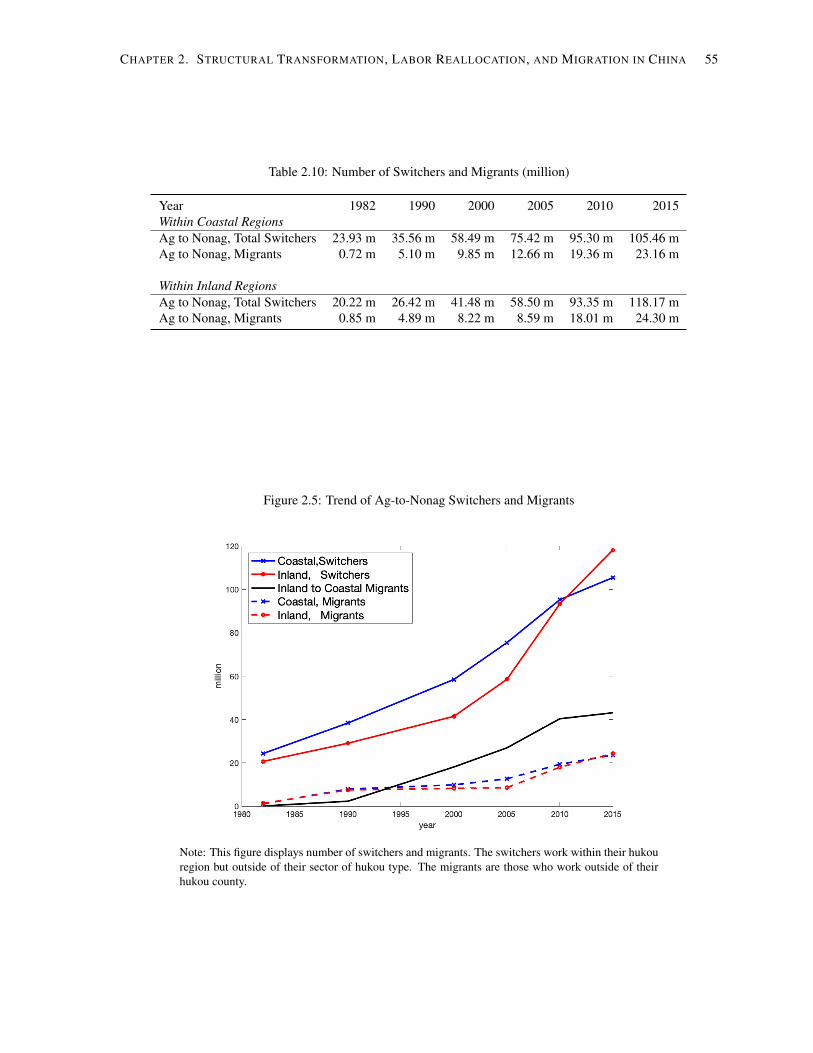
CHAPTER 2. STRUCTURAL TRANSFORMATION, LABOR REALLOCATION, AND MIGRATION IN CHINA 55
Table 2.10: Number of Switchers and Migrants (million)
Year 1982 1990 2000 2005 2010 2015Within Coastal RegionsAg to Nonag, Total Switchers 23.93 m 35.56 m 58.49 m 75.42 m 95.30 m 105.46 mAg to Nonag, Migrants 0.72 m 5.10 m 9.85 m 12.66 m 19.36 m 23.16 m
Within Inland RegionsAg to Nonag, Total Switchers 20.22 m 26.42 m 41.48 m 58.50 m 93.35 m 118.17 mAg to Nonag, Migrants 0.85 m 4.89 m 8.22 m 8.59 m 18.01 m 24.30 m
Figure 2.5: Trend of Ag-to-Nonag Switchers and Migrants
Note: This figure displays number of switchers and migrants. The switchers work within their hukouregion but outside of their sector of hukou type. The migrants are those who work outside of theirhukou county.

CHAPTER 2. STRUCTURAL TRANSFORMATION, LABOR REALLOCATION, AND MIGRATION IN CHINA 56
Table 2.11: Alternative Definition of Within-Region Migration
Year 1982 1990 2000 2005 2010 2015Panel A: Mover/Switcher CostsCross Sectors & Within Region(1)Ag to Nonag, Coastal 204.61 41.10 47.38 38.09 23.74 16.74(2)Ag to Nonag, Inland 320.63 85.57 79.54 77.85 39.41 17.95(3)Nonag to Ag, Coastal 85.64 22.16 8.91 9.33 11.86 22.81(4)Nonag to Ag, Inland 43.47 15.58 7.37 8.34 7.96 7.32
Cross Sectors & Between Regions(5)Ag to Nonag, Inland to Coastal 1957.52 219.88 77.11 57.07 33.25 19.71(6)Ag to Nonag, Coastal to Inland 1025.04 114.61 152.79 174.48 96.55 36.17(7)Nonag to Ag, Inland to Coastal 324.45 41.05 27.72 34.25 38.65 190.20(8)Nonag to Ag, Coastal to Inland 350.96 84.47 24.88 29.41 39.70 101.60
Same Sector & Between Regions(9)Ag to Ag, Inland to Coastal 237.02 73.89 73.78 97.62 78.07 94.66(10)Ag to Ag, Coastal to Inland 173.04 57.63 77.17 106.93 71.28 61.60(11)Nonag to Nonag, Inland to Coastal 107.71 23.66 17.93 12.52 10.39 8.11(12)Nonag to Nonag, Coastal to Inland 105.42 44.52 23.17 21.18 15.89 15.09
Panel B: Decomposing the Effect of Mover/Switcher Cost ChangesOverall 0.00% -3.32% -6.25% -6.97% -7.77% -7.51%
Cross Sectors & Within Region(1)Ag to Nonag, Coastal 0.00% -0.86% -0.76% -0.67% -0.74% -0.71%(2)Ag to Nonag, Inland 0.00% -1.65% -0.93% -0.83% -1.42% -1.61%(3)Nonag to Ag, Coastal 0.00% 0.02% 0.12% 0.16% 0.15% 0.01%(4)Nonag to Ag, Inland 0.00% 0.01% 0.05% 0.04% 0.07% 0.01%
Cross Sectors & Between Regions(5)Ag to Nonag, Inland to Coastal 0.00% -0.65% -4.23% -4.91% -5.10% -4.21%(6)Ag to Nonag, Coastal to Inland 0.00% -0.14% -0.04% -0.02% -0.03% -0.07%(7)Nonag to Ag, Inland to Coastal 0.00% 0.01% 0.03% 0.03% 0.03% 0.00%(8)Nonag to Ag, Coastal to Inland 0.00% 0.00% 0.01% 0.01% 0.01% 0.00%
Same Sector & Between Regions(9)Ag to Ag, Inland to Coastal 0.00% -0.02% -0.01% -0.00% 0.01% 0.00%(10)Ag to Ag, Coastal to Inland 0.00% 0.00% 0.00% 0.00% 0.00% 0.00%(11)Nonag to Nonag, Inland to Coastal 0.00% -0.05% -0.57% -0.87% -0.89% -1.07%(12)Nonag to Nonag, Coastal to Inland 0.00% 0.01% 0.08% 0.10% 0.15% 0.15%
Note:1 This table presents result under a stricter within-region migration definition where only migrants are counted. Thewithin-region sole switchers that stay in their hukou county are counted into agriculture sector and pay no sectorswitching cost.2 ln(Y1982MigCost/Y ) measures the proportional output gain from the reduction in mover/switcher costs since 1982,where Y1982MigCost is the counterfactual case where mover/switcher costs are fixed to the initial 1982 level (hkl,i j,t =hkl,i j,1982).3 ‘Ag’ stands for agricultural sector and ‘Nonag’ is for nonagricultural sector.4 Within-region switchers work within their hukou region but outside of their sector of hukou type.5 Between-region migrant workers are those who work outside of their hukou region.

CHAPTER 2. STRUCTURAL TRANSFORMATION, LABOR REALLOCATION, AND MIGRATION IN CHINA 57
Table 2.10 and Figure 2.5 compare the number of within-region migrants under this narrower definition, withwithin-region total switchers under the original broad definition. Although the trends are similar, the within-regionmigrants are only 19% of the broad definition.
Table 2.11 panel A displays the mover/switcher costs under this narrower definition. On average, the within-region mover/switcher cost is 15 times higher than in the baseline case. Between-region mover/switcher costs arealso slightly higher because, as the number of stayers, the migrant-to-stayer ratio decreases, which drives up allmover costs.
Table 2.11 panel B reports the effect of the reduction in mover/switcher cost under the narrower definition(excluding sole switchers). The impact of the overall cost decline is two-thirds that of the baseline in 1990 andone-third that of the baseline in 2015. The average reduction in ag-to-nonag within-region mover/switcher cost isone-third that of the baseline, which suggests that sole switchers play an important role in economic growth. Inthis case, the inland agriculture to coastal nonagriculture mover/switcher cost (row (5)) is the largest cost since2000.
2.6 Conclusion
In Chapter 1, I document a series of labor market policies that reduce labor market barriers and lead to significantlabor reallocation and migration between the agricultural and nonagricultural sectors as well as the inland andcoastal regions over China’s reform period. Since the 1978 economic reform, workers first reallocated fromagriculture to nonagriculture within the inland and coastal regions, respectively. Since the 1990s, increasingnumbers of workers migrated from inland agriculture to coastal nonagriculture, comprising as much as 6% of thelabor force in 2015.
My two-region two-sector general equilibrium model, calibrated to a unique dataset I constructed, suggeststhrough counterfactual analysis that the reduction in all of China’s reallocation and migration costs since 1982contributed up to 26.5% of output in 2015. In particular, the decline in agriculture-to-nonagriculture reallocationcosts from three main channels – within coastal region, within inland region, and inland-to-coastal regions – eachcontributed around one-third of the output gain in 2015. While the reductions in within-region costs were moreimportant contributors to output than between-region reductions before 1990, this order reversed after 1990.
Despite China’s substantial gains from reducing its reallocation and migration barriers, there still remainssubstantial potential left on the table for further reduction in the remaining barriers. Eliminating all remaining mi-gration barriers, for example, would boost simulated output by 14% in 2015. Interestingly, potential output gainsrise and peak in 2000 before they decline. This is because, between 1982 and 2000, the growth in migration andlabor reallocation was not sufficient to catch up to the widening sectoral productivity gap. After 2000, thanks toeasing migration restrictions, workers became more mobile and the productivity gap became stable. Importantly,the heaviest migration barrier impeded movement from inland agriculture to coastal nonagriculture – which canbe a vital point of focus for future migration policy in order to minimize labor misallocation and promote growth.
A few aspects of this chapter can be improved. First, I assume that workers are homogeneous in my model.However, workers of different gender, age, and skill levels may face different mover/switcher costs. Gai et al.(2021) models heterogeneous migration costs, not only across locations but also for individuals with differentcharacteristics. They find that migration costs are lower for men, highly educated workers, and younger workers.I leave the consideration of worker heterogeneity to future research. Second, I assume that sector-region-specificlabor productivities are exogenous and are not affected by labor reallocation and migration. If production tech-nologies use land as a fixed factor and/or if there are regional comparative advantage and trade, as in Tombe and

CHAPTER 2. STRUCTURAL TRANSFORMATION, LABOR REALLOCATION, AND MIGRATION IN CHINA 58
Zhu (2019), there could be diminishing returns to labor reallocation and migration. This may induce smalleraggregate productivity gains from lower mover/switcher barriers than those estimated in this chapter. The effectof introducing physical capital into production technologies is ambiguous and depends on the interaction betweencapital market distortions and labor market barriers. In the next chapter, a much richer model will be used to exam-ine the effects of changes in mover/switcher costs. The model allows for land and physical capital in productiontechnologies, regional comparative advantage and trade, and capital market distortions.

CHAPTER 2. STRUCTURAL TRANSFORMATION, LABOR REALLOCATION, AND MIGRATION IN CHINA 59
2.7 Appendix
2.7.1 Output Data
To construct real GDP for each province and sector, I use information on nominal GDP levels and real GDPgrowth rates (from CSY) and price level differences in 1990 (from Brandt and Holz (2006)). I first constructthese three series for each province and for the agricultural and nonagricultural sectors. Then I aggregate theprovincial-level nominal and real GDP into coastal and inland regions. 6
Note that administrative changes in provincial borders do not affect my regional data. In 1988, Hainan sepa-rated from Guangdong province and become an independent province. In 1997, Chongqing municipality separatedfrom Sichuan province. In the following analysis, I calculate the real GDP of each province separately and thenaggregate provinces into regions. Tibet starts reporting GDP data in 1984. Since Tibet has small population andGDP, I follow the literature in removing it from all data series.
2.7.1.1 Nominal GDP and Real GDP Growth Rate
The CSY reports nominal GDP in levels and real GDP growth rate for each province, but not real GDP in levels.These are reported for primary (agriculture), secondary (manufacturing, mining, construction, and utilities), andtertiary (service) sectors. I treat the primary sector as the agricultural sector and the secondary and tertiary sectorsin aggregate as the nonagricultural sector.
The nominal GDP and real GDP growth rate are subject to revision by the National Bureau of Statistics ofChina (NBS). In the 1995 CSY, the NBS revised up national tertiary sector nominal GDP and real growth rates ofall years back to 1978, following the 1993 Tertiary Sector Census. Specifically, tertiary sector GDP was revisedupward by 4.37% in 1978 and 32.04% in 1993 Holz (2006, P13, Line 65). Another revision following the 2004Economic Census revised 1993-2004 nominal values and real growth rates for the three main sectors as well asnationwide. Fortunately, the two revisions at the provincial level are reflected in the Gross Domestic Product ofChina (GDPoC) 1952-95 and GDPoC 1952-2004, respectively. Therefore, to incorporate the two major revisionson nominal GDP and real GDP growth rate, I employ the revised 1978-93 and 1993-2004 provincial and sectoraldata from GDPoC 1952-95 and GDPoC 1952-2004, respectively. Post-2004 nominal GDP at the province andsector level are from the 2005-2015 annual CSY.
Additionally, some revisions are reported at only the national level. Following the 2013 Economic Census,the NBS applied minor revisions to GDP data for all years back to 1978 in the 2015 CSY. Besides, China’s NBSretrospectively revises the last previously published annual data Holz (2006, P11, Line 57). I therefore consult the2016 yearbook for any updated official national GDP figures. 7
Moreover, aggregation of province-level nominal GDP routinely exceeds the reported national nominal GDPfor each of the primary, secondary, and tertiary sectors Holz (2006, P10, Line 50). To render the provincial-levelnominal GDP measures consistent with national GDP figures, I proportionally rescale provincial data to the 2016national benchmark such that the provincial sum equals the national total by assuming that provincial GDP sharesremain unchanged.
6The coastal region: Beijing, Tianjin, Hebei, Liaoning, Shanghai, Jiangsu, Zhejiang, Fujian, Shandong, Guangdong, and Hainan Province.The inland region: Shanxi, InnerMongolia, Jilin, Heilongjiang, Anhui, Jiangxi, Henan, Hubei, Hunan, Guangxi, Chongqing, Sichuan,Guizhou, Yunnan, Tibet, Shaanxi, Gansu, Qinghai, Ningxia, and Xinjiang Province.
7At the national level, the 2013 Economic Census revised nominal GDP for each of three sectors: On average, the primary sector wasrevised down by around 1%, the secondary sector was revised up by 0.05%, and the tertiary sector was revised up by 3%.

CHAPTER 2. STRUCTURAL TRANSFORMATION, LABOR REALLOCATION, AND MIGRATION IN CHINA 60
2.7.1.2 Deflator
GDP deflator can be calculated from nominal GDP, real GDP growth rate, and price level differences in 1990. Thegrowth rate of the GDP deflator is given by the ratio of nominal to real GDP growth rates for each province andsector. However, this deflator only shows price differences across time and remains incomparable across provincesand sectors. Brandt and Holz (2006) constructs the cost of provincial and urban-rural consumption baskets. Tocompare price level differences across provinces and sectors in our base year 1990, I set the 1990 GDP deflatorequal to each provinces’ cost of a common basket of goods relative to the national average. In the base year, I usethe common basket price index for rural areas to deflate agriculture’s nominal GDP in each province and use thecommon price index for urban areas to deflate nonagriculture’s nominal GDP.
One potential issue with using the rural and urban price index as the agriculture and nonagricultural price inthe base year is that real nonagricultural output in rural areas may be measured imprecisely. This is because, whilethe agricultural good is produced solely by rural workers, the nonagricultural good is produced in both rural andurban areas. 8 Assigning the urban price index to nonagriculture in the base year assumes this urban price is facedby all nonagriculture producers. This is inaccurate because the portion of nonagricultural goods produced in ruralarea should be deflated with rural prices, which are lower than urban prices. Therefore, employing the urban priceindex to calculate the real nonagricultural output would underestimate the overall real nonagricultural output.
Figure 2.6: Price Trend by Region and Sector
Note: The region and sector specific price is the ratio of their nominal and real GDP.
The real GDP of each region and sector is its nominal GDP divided by the price index. I then aggregate theprovincial-level nominal and real GDPs by coastal and inland region. The region and sector specific price is theratio of their nominal and real GDP.
8The rural nonagricultural good is produced by rural Township and Village Enterprises (TVEs), rural private firms, and rural self-employedworkers

CHAPTER 2. STRUCTURAL TRANSFORMATION, LABOR REALLOCATION, AND MIGRATION IN CHINA 61
2.7.2 Proof of Migration Share
Proposition:
Given the real consumption level for each region and sector Ci j, mover/switcher costs between all region/sectorpairs hkl,i j and a Frechet distribution Fe(x) of the heterogeneous preferences, the share of originally kl workerswho change to destination i j is
mkl,i j =Lkl,i j
Lkl=
(Ci j/hkl,i j)k
Âi0 Â j0(Ci0 j0/hkl,i0 j0)k (2.13)
where Lkl is the total number of originally kl workers.
Proof. The share of people migrate from region/sector kl to i j is the probability that one’s utility in i j exceedsthat in any other region/sector:
mkl,i j = Pr✓
ei jCi j/hkl,i j � maxi0 j0
{ei0 j0Ci0 j0/hkl,i0i0}◆.
By assumption, the idiosyncratic term ei j follows Frechet distribution with CDF Fe(x) = e�x�k . Let X =
ei jCi j/hkl,i j, then
Pr (X x) =Pr�ei jCi j/hkl,i j x
�
=Pr�ei j xhkl,i j/Ci j
�
=e�(x/sX )�k
where sX =Ci j/hkl,i j is simplified as a Frechet parameter. Next, let Y = maxi0 j0
{ei0 j0Ci0 j0/hkl,i0i0}.
Pr (Y x) =Pr✓
maxi0 j0
{ei0 j0Ci0 j0/hkl,i0i0} x◆
=’i0 6=i
’j0 6= j
Pr�ei0 j0Ci0 j0/hkl,i0i0 x
�
=’i0 6=i
’j0 6= j
Pr�ei0 j0 xhkl,i0i0/Ci0 j0
�
=’i0 6=i
’j0 6= j
e�(xhkl,i0i0/Ci0 j0 )�k
=e�x�k Âi0 6=i  j0 6= j(hkl,i0i0/Ci0 j0 )�k
=e�(x/sY )�k

CHAPTER 2. STRUCTURAL TRANSFORMATION, LABOR REALLOCATION, AND MIGRATION IN CHINA 62
where sY = (Âi0 6=i  j0 6= j(Ci0 j0/hkl,i0 j0)k)1/k . By law of probability, the migration share from kl to i j is:
mkl,i j =Z •
0Pr (X � Y |Y = y) fY (y)dy
=Z •
0(1�FX (y))
∂FY (y)∂y
dy
=Z •
0
∂FY (y)∂y
dy�Z •
0FX (y)
∂FY (y)∂y
dy
=1�Z •
0e�(y/sX )
�k kskY y�k�1e�(y/sY )
�kdy
=1�Z •
0e�y�k (sk
X+skY ) ksk
Y y�k�1dy
Let u = y�k and therefore du = ky�k�1. The above equation countinous as:
mkl,i j =1+Z u=0
u=•e�u(sk
X+skY ) sk
Y dy
=1� skY
Z •
0e�u(sk
X+skY )dy
=1� skY
skX + sk
Y
=sk
Xsk
X + skY
=(Ci j/hkl,i j)k
Âi0 Â j0(Ci0 j0/hkl,i0 j0)k
which is the result. The third step follows integralR •
0 e�axdx = 1a .
2.7.3 Construct Mover/Switcher Matrix
This subsection presents the strategy to reconcile the sectoral employment discrepancy between the CSY andcensus. Chapter 1 Section 1.4.1 documents that this sectoral employment discrepancy is likely due to differentdefinitions of sectoral employment. (Yue, 2005) suggests that the CSY definition is believed to be more accurate.Therefore, I use labor reallocation and migration information from the census and regional employment in theCSY to estimate the mover/switcher matrix. The detailed steps are as follows.
First, the census samples report workers’ current location and sector as well as their hukou location and type.Assuming that individuals with rural (urban) hukou work initially in agriculture (nonagriculture), each individ-ual’s initial (origin), current (destination) location, and work sector falls into one of four region/sectors: coastalagriculture, coastal nonagriculture, inland agriculture, and inland nonagriculture. These four region/sectors,representing origins and destinations, constitute the sides of a 4x4 matrix of bilateral mover/switcher levelsLkl,i j (k, i = a,n, l, j = c,d, c for coastal and d for inland) that shows the number of workers who change fromregion/sector kl to i j. This mover/switcher matrix is represented as follows:

CHAPTER 2. STRUCTURAL TRANSFORMATION, LABOR REALLOCATION, AND MIGRATION IN CHINA 63
Destination i j :ca cn da dn
0
BBB@
1
CCCA
ca Lca,ca Lca,cn Lca,da Lca,dn
Origin kl : cn Lcn,ca Lcn,cn Lcn,da Lcn,dn
wa Lda,ca Lda,cn Lda,da Lwa,dn
wn Ldn,ca Ldn,cn Ldn,da Lwn,dn
Each row of this mover/switcher matrix sums up to origin region/sector employment Lkl(= Âi j Lkl,i j). Eachcolumn sums up to destination region/sector employment Li j(= Âkl Lkl,i j).
Second, equation (2.6) can be used to convert the mover/switcher levels matrix to a mover/switcher sharesmatrix M, where each element mkl,i j shows the share of originally kl workers who change to region/sector i j:
Destination i j :ca cn da dn
0
BBB@
1
CCCA
ca mca,ca mca,cn mca,da mca,dn
Origin kl : cn mcn,ca mcn,cn mcn,da mcn,dn
wa mda,ca mda,cn mda,da mwa,dn
wn mdn,ca mdn,cn mdn,da mwn,dn
Third, I use the CSY sectoral employment Li j and census mover/switcher shares matrix M to deduce the originworker count:
0
BBBB@
mca,ca mcn,ca mda,ca mdn,ca
mca,cn ... ... ...
mca,da ... ... ...
mca,dn ... ... ...
1
CCCCA
M0(known)
0
BBBB@
ˆLcaˆLcnˆLdaˆLdn
1
CCCCA
Origin Workers(unknown)
=
0
BBBB@
Lca
Lcn
Lda
Ldn
1
CCCCA
Destination Workers(known)
Fourth, I estimate the mover/switcher matrix by applying the mover/switcher shares matrix M to the deducedorigin worker count Li j. Specifically, the element of this estimated mover/switcher matrix is Lkl,i j = ˆLkl ⇤mkl,i j.The column sum of this estimated mover/switcher matrix is the same employment Li j in the CSY.
Table 2.12 compares the deduced origin worker count ˆLi j to that directly from the census data Li j. In panelA, origin worker counts Li j are represented by their hukou region/sector directly from the census. Agriculturalhukou share is relatively constant over time. Panel B presents the deduced origin worker counts ˆLi j. The deducednonagricultural worker count is larger than that in the census. This is because, for a given migration share matrix,we need to assume more nonagricultural workers in the origin in order to have more nonagricultural workers inthe destination, as suggested by the CSY. This is evident, especially in later years.
2.7.4 Additional Tables

CHAPTER 2. STRUCTURAL TRANSFORMATION, LABOR REALLOCATION, AND MIGRATION IN CHINA 64
Table 2.12: Origin Worker Counts (million)
Year 1982 1990 2000 2005 2010 2015Panel A: Census Origin Worker Counts
Lca 156.14 m 189.96 m 202.39 m 202.11 m 203.87 m 189.20 mLcn 47.25 m 50.30 m 65.17 m 69.17 m 77.38 m 100.24 mLda 267.41 m 338.30 m 371.66 m 387.48 m 384.14 m 351.31 mLdn 55.37 m 68.93 m 81.63 m 87.72 m 95.67 m 133.76 m
Agri hukou share 80.50% 81.59% 79.64% 78.98% 77.26% 69.79%Coastal hukou share 38.65% 37.11% 37.12% 36.34% 36.95% 37.37%
Panel B: Deduced Origin Worker CountsˆLca 145.51 m 153.62 m 145.98 m 145.62 m 143.52 m 133.48 mˆLcn 62.30 m 95.31 m 110.33 m 120.70 m 131.09 m 147.40 mˆLda 245.62 m 286.92 m 285.83 m 286.90 m 281.12 m 260.58 mˆLdn 72.75 m 111.64 m 178.72 m 193.25 m 205.32 m 233.05 m
Agri hukou share 74.33% 68.04% 59.90% 57.94% 55.80% 50.88%Coastal hukou share 39.50% 38.45% 35.56% 35.68% 36.08% 36.27%
Note: Panel A presents the origin worker counts given by the census. Panel B presents the origin workercounts deduced from census mover/switcher share matrix M and CSY employment.

CHAPTER 2. STRUCTURAL TRANSFORMATION, LABOR REALLOCATION, AND MIGRATION IN CHINA 65
Table 2.13: Including Hukou Changers as Within-Region Mover/Switcher
Year 1982 1990 2000 2005 2010 2015Panel A: Mover/Switcher CostsCross Sectors & Within Region(1)Ag to Nonag, East 23.33 11.62 10.53 7.85 5.06 2.73(2)Ag to Nonag, West 48.26 28.61 20.79 16.39 9.56 4.70(3)Nonag to Ag, East 1.05 1.78 0.91 0.96 1.28 1.92(4)Nonag to Ag, West 0.51 1.13 0.78 0.68 0.73 1.09
Cross Sectors & Between Regions(5)Ag to Nonag, West to East 1861.27 210.13 72.06 51.52 27.89 15.11(6)Ag to Nonag, East to West 919.94 101.32 125.69 133.24 67.53 22.76(7)Nonag to Ag, West to East 304.91 36.98 23.08 27.10 29.80 141.99(8)Nonag to Ag, East to West 340.82 76.48 20.89 23.94 31.44 77.77
Same Sector & Between Regions(9)Ag to Ag, West to East 225.37 70.61 68.95 87.47 65.48 72.59(10)Ag to Ag, East to West 155.30 50.95 63.49 80.20 49.86 38.76(11)Nonag to Nonag, West to East 101.22 21.31 14.93 10.00 8.01 6.06(12)Nonag to Nonag, East to West 102.38 40.31 19.45 17.16 12.58 11.55
Panel B: Decomposing the Effect of Mover/Switcher Cost ChangeOverall 0.00% -6.45% -11.99% -16.52% -23.75% -30.28%
Cross Sectors & Within Region(1)Ag to Nonag, Coastal 0.00% -2.50% -4.23% -5.95% -8.07% -9.67%(2)Ag to Nonag, Inland 0.00% -2.41% -3.06% -4.20% -6.30% -7.95%(3)Nonag to Ag, Coastal 0.00% -0.36% 0.17% 0.12% -0.25% -0.69%(4)Nonag to Ag, Inland 0.00% -0.63% -0.61% -0.49% -0.65% -1.36%
Cross Sectors & Between Regions(5)Ag to Nonag, Inland to Coastal 0.00% -0.41% -3.70% -5.08% -7.47% -9.08%(6)Ag to Nonag, Coastal to Inland 0.00% -0.07% -0.01% -0.01% -0.06% -0.31%(7)Nonag to Ag, Inland to Coastal 0.00% 0.00% 0.00% 0.00% 0.00% 0.00%(8)Nonag to Ag, Coastal to Inland 0.00% 0.00% 0.00% 0.00% 0.00% 0.00%
Same Sector & Between Regions(9)Ag to Ag, Inland to Coastal 0.00% -0.03% -0.04% -0.02% -0.04% 0.00%(10)Ag to Ag, Coastal to Inland 0.00% 0.01% 0.01% 0.00% 0.03% -0.01%(11)Nonag to Nonag, Inland to Coastal 0.00% -0.06% -0.57% -0.96% -1.04% -1.31%(12)Nonag to Nonag, Coastal to Inland 0.00% 0.01% 0.05% 0.06% 0.10% 0.11%
Note:1 This table presents main result from migration matrix that count hukou changers as migrants from the same region. Thenumber of hukou changers is an upper bound of the ideal number of workers who changed hukou type. So this table showsthe lower bound of mover/switcher costs and upper bound of output gain.2 ln(Y1982MigCost/Y ) measures the proportional output gain from the reduction in mover/switcher costs since 1982, whereY1982MigCost is the counterfactual case where mover/switcher costs are fixed to the initial 1982 level (hkl,i j,t = hkl,i j,1982).3 ‘Ag’ stands for agricultural sector and ‘Nonag’ is for nonagricultural sector.4 Within-region switchers work within their hukou region but outside of their sector of hukou type.5 Between-region migrant workers are those who work outside of their hukou region.

Chapter 3
The Effect of Migration Policy on Growth,Structural Change, and RegionalInequality in China, 2000-20151
1This chapter is a slightly modified version of a joint work with Ruiqi Sun, Trevor Tombe, and Xiaodong Zhu published in the August2020 issue of Journal of Monetary Economics.
66

CHAPTER 3. MIGRATION POLICY ON GROWTH, STRUCTURAL CHANGE, AND INEQUALITY IN CHINA 67
3.1 Introduction
China’s economic growth since 2000 has been impressive. And although less well known, its rapid structuralchange and large regional income convergence are no less remarkable. Between 2000 and 2015, while the coun-try’s aggregate GDP per worker quadrupled, the share of employment in agriculture fell in half and the incomeinequality across provinces fell by a third. Worker reallocation and migration is central to this transformation.The number of workers switching sectors and/or migrating outside their area of hukou registration increased fromaround 110 million in 2000 to almost 300 million in 2015, mostly due to changes in policies that made laborreallocation and migration easier. In this paper, we quantify the impact of migration policy changes on China’sgrowth, structural change, and regional income convergence.
To accomplish this, we compile uniquely detailed data on production, capital, employment, trade, sectorallabor reallocation, and migration in China. These data reveal four key facts concerning China’s structural changeand regional convergence. First, there was significant regional convergence in real GDP per worker between 2000and 2015. The variance of the cross-province (log) GDP per worker declined by a third, from 0.24 in 2000 to 0.15in 2015. Second, over the same period, there were little convergence in GDP per worker within the agriculturaland nonagricultural sectors. Third, structural change was an important contributor to growth and convergence.The fraction of employment in agriculture fell from 53% in 2000 to 28% in 2015. The largest changes occurredin provinces with lower initial levels of income, higher initial shares of agricultural employment, and larger gapsin labor productivity between the agricultural and nonagricultural sectors. Therefore reallocation of labor fromagricultural to the nonagricultural sector (ag-to-nonag) resulted in larger increases in aggregate GDP per workerin poor provinces than in richer provinces and contributed significantly to the convergence in aggregate incomeacross provinces. Fourth, the structural change is closely related to inter-provincial migration. Provinces withhigher shares of employment in agriculture in 2000 had larger inter-provincial ag-to-nonag reallocation. Thesefacts suggest that labor reallocation and migration-induced structural change is essential for China’s growth andregional income convergence between 2000 and 2015.
We bring our data to a rich yet tractable spatial equilibrium model of China’s economy to both measurechanges in labor market frictions and other frictions in China’s economy and to quantify their impacts on structuralchange, growth, and regional income convergence. We find that, between 2000 and 2015, the costs of migrationand switching sectors (hereafter, mover/switcher costs) fell by forty-five percent, with the cost of ag-to-nonagswitching falling even more. In addition to contributing to growth, these mover/switcher cost changes accountfor the majority of the reallocation of workers out of agriculture and the drop in regional income inequality. Wecompare the effect of migration policy changes with other important economic factors, including changes in tradecosts, capital market distortions, average cost of capital, and productivity. While each contributes meaningfully togrowth, migration policy changes are central to China’s structural change and regional convergence. Finally, wefind that the slow-down in growth between 2010 and 2015 is associated with a smaller reduction in inter-provincialmover/switcher costs and a larger role of capital accumulation during this five-year period.
Our model builds on recent developments in international trade. In particular, we extend the Eaton and Kortum(2002) model to multi-sector as in Caliendo and Parro (2015) and incorporate both imperfect spatial and sectorlabor mobility as in Tombe and Zhu (2019). In addition, we allow for capital as an input in production andfrictions in capital allocation across space and sectors. To better identify inter-sector switching costs, we alsoconsider household preferences that are non-homothetic to control for the impact of income growth on ag-to-nonag reallocation.
Our work contributes to the literature investigating the effect of China’s hukou system, and recent reforms to it.Most recently, Zi (2020) explores the effect of internal frictions in China’s labor market on how trade liberalization

CHAPTER 3. MIGRATION POLICY ON GROWTH, STRUCTURAL CHANGE, AND INEQUALITY IN CHINA 68
improves welfare. In particular, hukou restrictions tend to dampen the gains from trade. On the other hand, Tian(2018) finds that the external trade liberalization associated with China’s accession to WTO induced some ofthe migration policy changes and amplified the impact of external trade liberalization on internal migration inChina. Estimating hukou restrictions at the prefecture-level, Ma and Tang (2019) find significant welfare gainsfrom easing labor mobility restrictions. Finally, Kinnan et al. (2018) use China’s “sent-down youth” program toidentify exogenous effect of migration and find migration lowers consumption volatility and asset-holding. Ourwork is distinct not only methodologically, but also in that we focus on a longer period of time, from 2000 to2015, and examine the impact of migration policy changes on growth, structural change, and regional inequalityat the same time in a unified model with endogenous and frictional labor, capital, and production allocations.
Our work also builds on a large and growing literature quantifying the effects of internal migration (Caliendoet al., 2017; Schmutz and Sidibe, 2018; Imbert and Papp, 2019; Heise and Porzio, 2019). Most recently, Bryanand Morten (2019) show that internal labor migration in Indonesia has significant implications for aggregateproductivity there. Reducing migration costs to the U.S. level boosts aggregate productivity by 7.1%. Our workalso connects with those investigating the link between trade and migration or structural change. Of particularrelevance for China, Fan (2019) demonstrates that trade may exacerbate inequality, and Erten and Leight (2017)analyze the effect of China’s accession to WTO in 2001 on structural change at the local level.
By linking reallocation of labor across sectors to migration, we contribute to the large literature on structuralchange (Herrendorf et al., 2014) and the agricultural productivity gaps (Gollin et al., 2014). Given such gapsin labor productivity between sectors, shifting labor from agriculture to nonagriculture can significantly boostaggregate productivity. Our emphasis on the role of structural change in regional income convergence is alsodirectly related to Caselli and Coleman II (2001), who study structural change and income convergence in theUS. We document that the central factors behind China’s structural transformation are labor reallocation withinprovinces and migration between provinces. Eckert and Peters (2018) also examine the interaction betweenmigration and structural change. But, unlike for China, they find regional migration contributed little to thedecline in the agriculture’s share of employment in the United States. Finally, we build on the recent work of Alderet al. (2019), Comin et al. (2015), and Boppart (2014), by allowing for income effect (through non-homotheticpreferences) to be a driver of structural change. We find income effect magnifies the impact of reductions inmover/switcher costs on structural change and growth. We also show that ignoring income effect may lead one tooverestimate both the initial levels of and reductions in switching and migration costs.
Finally, our paper is closely related to and build on the work by Tombe and Zhu (2019). We extend their worktheoretically by incorporating into the model physical capital as an input in production and income effect throughnon-homothetic preferences. We also extend their work empirically by extending their analysis of the impact oftrade, labor reallocation, and migration on China’s growth between 2000 and 2005 to a much longer and morerecent period, from 2000 to 2015. Most important, we go beyond their analysis on aggregated GDP growth bystudying the impact of mover/switcher cost changes and other changes on both structural change and regionalincome inequality in China.
We begin our analysis with a detailed review of the data in Section 3.2, where we document key patterns inChina’s regional economic growth, structural change, labor reallocation, and migration between 2000 and 2015.With the data in hand, we develop a rich model of China’s economy that can be brought to the data in Section3.3. We then use this model to quantify the magnitude and consequence of changes in mover/switcher costs, tradecosts, capital market distortions, and productivity. We document the results of this quantitative analysis in Section3.4 before concluding in Section 3.5.

CHAPTER 3. MIGRATION POLICY ON GROWTH, STRUCTURAL CHANGE, AND INEQUALITY IN CHINA 69
3.2 Sectoral Labor Reallocation, Migration, Structural Change, and Re-gional Income Convergence
In this section, we document large income disparity across provinces and between the agricultural and nonagri-cultural sectors in China in 2000, and the significant regional income convergence and structural change between2000 and 2015. We also provide evidence suggesting that the structural change and regional income convergenceare intimately related. We then discuss the migration policy changes and the resulting increases in labor realloca-tion and migration as an important driver for both the structural change and regional income convergence. First,however, we discuss briefly the data we use for the paper.
3.2.1 Data
For our analysis, we combine three sources of data on internal labor reallocation and migration, internal andinternational trade, and provincial economic accounts in China. We briefly list the important variables here, andprovide a more thorough description in the appendix.
Sectoral Labor Reallocation and Migration. Our labor reallocation and migration data are from China’spopulation census. In addition to the 2000 and 2005 census data used by Tombe and Zhu (2019), we also use theconfidential micro data of the 2010 and 2015 population census of China.2 These census data provide detailedinformation about sectoral labor reallocation and cross-province migration from 2000 to 2015.
Trade. We construct inter-provincial trade flows based on the inter-provincial input-output table for 2002,2007, and 2012 from Li (2010), Liu et al. (2012), and Liu et al. (2018), respectively.
Provincial GDP and Employment. We construct provincial GDP, capital stock, and employment for agricul-ture and nonagriculture based mainly on the data published in the China Statistical Yearbook (CSY) by China’sNational Bureau of Statistics (NBS). The construction methods for GDP and employment are the same as inTombe and Zhu (2019). However, after 2010, the NBS no longer publishes provincial level employment bysector. For 2015, we therefore estimate provincial employment based on the data published in the provincialyearbooks. We describe the full estimation procedure in the appendix.
Provincial Capital Stock. The CSY reports nominal Gross Fixed Capital Formation (GFCF) by provincebut not by sector. However, it does report the fixed-asset investment by province and sector. We approximateeach sector’s share of capital formation by using the sector’s share of total fixed-asset investment. The realinvestment is nominal GFCF deflated using the province-specific investment price index reported in the CSY. Wethen construct capital stock using a perpetual inventory method assuming a depreciation rate of 7%. The averageinvestment growth rates of the first ten years of a province are used to generate initial capital stock values for 1978.Our estimates of annual real investment, less depreciation, are then used to calculate capital stock in subsequentyears.
3.2.2 Factor Return Dispersion across Provinces and Sectors
Tombe and Zhu (2019) document large differences in real labor income across provinces and between the agricul-tural and nonagricultural sectors in China in 2000, and they argue that an important reason for these differences isthe hukou system that imposes severe restrictions on worker mobility within China. Here we show the evolutionof the distribution of real returns to labor across provinces and sectors over the 15-year period after 2000.
2These data are from NBS micro survey databases: 2010 China Population Census Mirco-database and 2015 1% Sample China PopulationCensus Mirco-database.

CHAPTER 3. MIGRATION POLICY ON GROWTH, STRUCTURAL CHANGE, AND INEQUALITY IN CHINA 70
Using data on real GDP, employment, and factor shares, the real marginal return to labor is
w jn = ab j,l Y j
n
L jn, (3.1)
where Y jn is real GDP of sector j in province n, L j
n is employment, b j,l is labor’s share of value-added, and a isthe share of non-housing goods and services in GDP. We display the distribution of real marginal returns to laborfor 2000, 2005, 2010, and 2015 in Figure 3.1a, which reveals persistent within-sector dispersion of labor returnsacross provinces and large gaps between agriculture and the nonagriculture. Only in the last five years, between2010 and 2015, did the within-sector dispersion in returns and the between sector gaps in returns decline slightly.
For comparison, we also report the distribution of returns to capital across provinces and sectors in Figure3.1b. Specifically, the returns to capital in province n and sector j is
r j,kn = ab j,k P j
nY jn
K jn
, (3.2)
where b j,k denotes capital’s (k) share of value-added and P jnY j
n the nominal GDP of sector j in province n. Notethat we examine nominal rather than real returns to capital because capital owners can invest across locationsand sectors without having to consume at the investment destinations. Therefore they care about nominal returndifferences only and the differences in the cost of living across locations and sectors do not directly affect theirinvestment decisions. If there are no capital market frictions, then investors’ arbitrage would imply that thenominal returns r j,k
n equalize across all sectors and provinces. So, the dispersion in the nominal returns to capitalreflects frictions that result in capital misallocation. As illustrated in Figure 3.1b, the dispersion of capital returnsacross provinces was persistently large in agriculture, but significantly smaller in the nonagricultural sector. Therewas a decline in the dispersion of capital returns in the nonagricultural sector between 2000 and 2005, but thedispersion then increased between 2010 and 2015. The Chinese government’s massive infrastructure and stimulusspending after the global financial crisis may have contributed to the worsening capital allocations during thatperiod, as pointed out by Bai et al. (2016).
3.2.3 Regional Income Convergence and Structural Change
While the within-sector dispersion in labor income did not show a significant decline between 2000 and 2015,there was a dramatic reduction in the inequality of the aggregate provincial labor income over the same period.The cross-province variance of log real GDP per worker was 0.24 in 2000. But by 2015, this variance declinedto 0.15 – a one-third reduction in regional income inequality. Behind this significant decline was the faster laborincome growth experienced by initially lower-income regions. In panel (a) of Figure 3.2, we display the growthrates of real GDP per worker between 2000 and 2015 of all the provinces against their initial real GDP per workerlevels in 2000. There is a significant negative relationship between the initial level of income and subsequentincome growth, implying strong income convergence over this 15-year period. Regressing the average growth oninitial real GDP per worker reveals a precisely estimated b�convergence coefficient of approximately 2%. Thatis, a 10% higher initial income level is associated with a 0.2% lower average annual growth rate.
What’s behind this reduction in regional inequality? In panel (b) of Figure 3.2, we plot the growth rates ofreal GDP per worker within each sector. The negative relationship between the growth rate and initial income isless significant, implying smaller within-sector convergence in real GDP per worker. In fact, the cross-provincevariances of log real GDP per worker within agricultural and the nonagricultural sectors were 0.20 and 0.12,

CHAPTER 3. MIGRATION POLICY ON GROWTH, STRUCTURAL CHANGE, AND INEQUALITY IN CHINA 71
Figure 3.1: Dispersion in Returns to Labor and Capital in China
(a) Real Returns to Labor
2010 2015
2000 2005
−3 −2 −1 0 1 2 −3 −2 −1 0 1 2
0
1
2
3
0
1
2
3
Log Relative Marginal Product of Labour
De
nsi
ty
Agriculture Non−Agriculture
(b) Nominal Returns to Capital
2010 2015
2000 2005
−3 −2 −1 0 1 2 −3 −2 −1 0 1 2
0
1
2
3
0
1
2
3
Log Relative Marginal Revenue Product of Capital
Densi
ty
Agriculture Non−Agriculture
Note: Panel (a) displays the dispersion of returns to labor across provinces, by sector, from 2000 to 2015. Panel (b) displaysthe dispersion in capital wedges over the same period.

CHAPTER 3. MIGRATION POLICY ON GROWTH, STRUCTURAL CHANGE, AND INEQUALITY IN CHINA 72
Figure 3.2: Convergence in Provincial Real GDP per Worker, 2000 to 2015
(a) Growth Rate in Total Real GDP per worker.0
4.0
6.0
8.1
.12
.14
Ave
rage A
nnual G
row
th R
ate
, 2000−
2015
−1 −.5 0 .5 1
Log GDP/Worker in 2000, Relative to Average
log(GDP/worker)
(b) Growth Rate in Ag and Nonag Real GDP per worker
.04
.06
.08
.1.1
2.1
4
Ave
rage A
nnual G
row
th R
ate
, 2000~
2015
−1 −.5 0 .5 1
Within Sector Log GDP/Worker in 2000, Relative to Average
Agriculture Non−agriculture
Note: These figures display the average annual growth rate in real GDP per worker in total, agriculture and nonagriculturefrom 2000 to 2015 against each province’s initial real GDP per worker in 2000. The negative relationship implies systematicconvergence across provinces, while convergences are much smaller within either of the two sectors.
respectively, in 2000, and 0.18 and 0.11 in 2015. In other words, there were only slight declines in within-sectorincome inequality. These facts suggest that changes in the sectoral composition of labor income or structuralchange must be an important reason for the convergence of aggregate GDP per worker across China’s provinces.
Structural change has been significant in China over this 15-year period, during which the share of employmentin agriculture fell nearly in half from 53% to 28%. Since labor productivity in agriculture is significantly lowerthan in nonagriculture, reallocation of labor towards the latter can increase a province’s overall labor productivity.Therefore, structural change can contribute to convergence in regional incomes if the pace of structural changewas faster in poor provinces than in rich provinces. And this is indeed the case. In panel (a) of Figure 3.3, wedisplay the change in the nonagricultural employment shares by province between 2000 and 2015. Provinces witha relatively small nonagricultural sector in 2000 (and therefore lower average income) saw significantly largeremployment shifts into this sector by 2015. Among those provinces with the smallest initial nonagriculturalemployment share (at or below 40%), nearly one-third of total provincial employment switched out of agriculture.Among those with the largest initial nonagricultural employment share (at or above 80%), only 10% of workersswitched. In addition, there is a relationship between structural change and a province’s agricultural productivitygap (the gap between the agricultural and nonagricultural real GDP per worker). In panel (b) of Figure 3.3, we plotthe initial agricultural productivity gap in 2000 by province against each province’s change in the nonagriculturalsector’s share of provincial employment between 2000 and 2015. With the exception of the six provinces withparticularly low levels of structural change (three municipalities, and three peripheral regions), there is a positiverelationship between the initial agricultural productivity gap and the pace of structural change.
To quantify in a simple way the degree to which structural change is driving regional convergence considerthe following simple decomposition of a province’s aggregate real GDP per worker,
yn,t = yagn,t + lna
n,t ·�yna
n,t � yagn,t�, (3.3)
where lagn,t is province n’s nonagricultural employment share in year t and y j
n,t is the real GDP per worker of sectorj in province n and year t. Holding each sector’s real GDP per worker fixed at their 2000 levels, we calculate the

CHAPTER 3. MIGRATION POLICY ON GROWTH, STRUCTURAL CHANGE, AND INEQUALITY IN CHINA 73
Figure 3.3: Structural Change across Provinces in China, 2000 to 2015
(a) Convergence in Economic Structure
Beijing
ShanghaiTianjin
0.05
0.10
0.15
0.20
0.25
0.30
0.35
0.2 0.4 0.6 0.8 1.0Non−agriculture employment share in 2000
Change in
Non−
Ag. E
mp. S
hare
, 200
0−
2015
(b) Agricultural Productivity Gap and Structural Change
Beijing
Heilongjiang
Liaoning ShanghaiTianjin
Xinjiang
0.05
0.10
0.15
0.20
0.25
0.30
0.35
0.5 1.0 1.5 2.0Nonag−to−Ag Real GDP per Worker Gap in 2000
Change in
Non−
Ag. E
mp. S
hare
, 200
0−
2015
Note: Panel (a) and (b) displays the change in the nonagricultural sector’s share of provincial employment between 2000 and 2015 against theinitial share in 2000 and the agricultural productivity gap in 2000, respectively.
counterfactual real GDP in province n as
yn,t = yagn,2000 + lna
n,t ·⇣
ynan,2000 � yag
n,2000
⌘. (3.4)
We find the variance of ln(yn) falls by one-quarter when only lnan,t is changing over time as in the data. Our simple
back-of-the-envelope calculation therefore suggests that structural change accounts for two-thirds of the observedconvergence between China’s provinces.
Of course, this simple calculation ignores potential endogenous relationships between the labor reallocationand the labor productivity in the two sectors, which we will take into account in our quantitative analysis ofa full general equilibrium model later. The simple calculation also does not tell us what drives the structuralchange. Next, we present evidence that ag-to-nonag worker reallocation within-provinces and migration between-provinces, can be important drivers of the structural change in China.
3.2.4 Sectoral Labor Reallocation and Migration in China
Before turning to the data on sectoral labor reallocation and migration, we first provide a summary of China’sinternal migration policy and recent changes to it. The Chinese government formally instituted a household reg-istration or hukou system in 1958 to control labor mobility. Chan (2019) provides a detailed and up-to-date dis-cussion of the system and its reforms. Briefly, each Chinese citizen is assigned a hukou, classified as “agricultural(rural)” or “nonagricultural (urban)” in a specific location. Individuals need approvals from local governments tochange the category (agricultural or nonagricultural) or location of hukou, and it is extremely difficult to obtainsuch approvals. In addition, prior to 2003, workers without local hukou had to apply for a temporary residencepermit. As the demand for migrant workers in manufacturing, construction, and labor intensive service industriesincreased, many provinces, especially the coastal provinces, eliminated the requirement of temporary residencepermit for migrant workers after 2003. There was also a nation-wide administrative reform in 2003 that greatlystreamlined the process for getting a temporary residence permit in other provinces. These policy changes madeit much easier for a worker to leave their hukou location and work somewhere else as a migrant worker. However,even with a temporary residence permit, migrant workers without local hukou have limited access to local public

CHAPTER 3. MIGRATION POLICY ON GROWTH, STRUCTURAL CHANGE, AND INEQUALITY IN CHINA 74
Table 3.1: Sectoral Labor Reallocation and Migration in China, 2000-2015
Intra-Provincial Inter-Provincial2000 2005 2010 2015 2000 2005 2010 2015
Total Switchers and Migrants Stock 101.5 132.6 176.2 215.7 29.7 47.0 79.2 90.2
Share of Employment (%)
Total Switchers and Migrants 14.1 17.8 22.9 28.0 4.1 6.5 10.3 11.7Ag-to-Nonag Switchers 13.0 16.5 21.6 25.5 3.3 5.2 8.6 7.0
Non-migrant Ag Workers 63.0 55.5 46.3 31.6 63.0 55.5 46.3 31.6Note: Displays the number of workers switching sectors and/or migrating outside their type or area of hukou registration. The first rowis in millions. The last three rows are shares of total employment.
services and face higher costs for health care and for their children’s education. In the late 1990s, a few localesbegan experimenting with eliminating the distinction between local agricultural/nonagricultural populations, pro-viding all local residents with a resident hukou entitling them equal access to local public services. This waseventually formalized and extended to the whole nation in 2014. At the same time, however, the government hastightened the requirement for granting hukou to migrants in the first- and second- tiered cities. So, over time, ithas become easier for a rural migrant worker to obtain hukou in a local urban area in lower tiered cities, but it hasbecome harder in recent years for them to move to large coastal cities due to the stricter restrictions there.
Based on population census data, we report in Table 3.1 both inter-provincial and intra-provincial switchersand migrants in China for the years of 2000, 2005, 2010, and 2015.3 As a reference, we also report the shareof workers who are non-migrant agricultural workers. A worker is defined as an inter-provincial migrant if theyworked outside their province of hukou registration. And they are defined as an intra-provincial switcher if theyworked within their province of registration but outside their sector of hukou registration. Our definition of intra-provincial switcher includes both switchers who stayed locally and those that migrated out of the area of theirhukou registration. We choose this definition because we find from the 2005 mini-census data that the averageincome of these local switchers is more than 2.5 times as high as that of the local farmers. This suggests thatthere are significant frictions for rural workers switching sectors locally. In our robustness analysis later, we willconsider a stricter definition of intra-provincial migrant workers.
As documented by Tombe and Zhu (2019), the relaxation of hukou restrictions on labor mobility between2000 and 2005 resulted in significant increases in labor reallocation and migration both intra- and inter-province.4
The general trend seems to have continued between 2005 and 2015, with the intra- and inter-provincial switcherand migrant’s shares of total employment increased from 17.8% and 6.5%, respectively, in 2005, to 28% and11.7% in 2015. Between 2010 and 2015, however, the increase in inter-provincial migration slowed significantly,and the cross-provincial migrants’ share of total employment in 2015 is actually lower than that in 2010. Incontrast, within-province ag-to-nonag switchers continued to increase significantly through 2015. These patternsare consistent with the policy changes adopted by the Chinese government after 2010 that have made moving totop tier cities, the destinations of much of the inter-provincial migration, much harder for people with rural hukouand, at the same time, encouraged local urbanization in poor inland and western provinces.
To see the impact of migration on structural change, in Figure 3.4, we plot for all the provinces their initial
3The switchers and migrants stocks are calculated from the census data and the total employment data are from the China StatisticalYearbook. This switchers and migrants total is slightly larger than that presented in Chapter 1 because here we use a slightly broadermover/switcher definition by including migrants who left their hukou county for less than six months.
4Our estimated switcher and migrant stocks are slightly different from those reported by Tombe and Zhu (2019) because we now use moredetailed sample weights provided by the NBS.

CHAPTER 3. MIGRATION POLICY ON GROWTH, STRUCTURAL CHANGE, AND INEQUALITY IN CHINA 75
Figure 3.4: Migration and Structural Change
0.0
5.1
.15
.2
Inte
r−pro
vinci
al A
g to N
a M
igra
tion S
hare
in 2
015
.2 .4 .6 .8 1
Non−ag Employment Share in 2000
Note: The figure displays the fraction of initially agriculturalworkers that now work in nonagricultural sectors, overall andout of province. This captures the relationship between migra-tion and structural change.
share of employment in agriculture in 2000 against their share of all the workers with agricultural hukou inthat province who work in the nonagricultural sector in another province in 2015. We can see that provinces withhigher shares of initial agricultural employment tend to have a larger proportion of workers move out of agricultureand into the nonagricultural sector outside their hukou registration provinces in 2015. Simply put, reductions inthe share of employment in agriculture in poor provinces are associated with inter-provincial out-migration offarmers.
In summary, the facts we document in this section suggest that migration policy changes and the associatedincreases in labor reallocation and migration have important effects on structural change and regional incomeconvergence in China between 2000 and 2015. We now turn to our main analysis that precisely quantifies theseeffects using a spatial general equilibrium model of trade, labor reallocation, and migration.
3.3 A Spatial Model of Trade, Labor Reallocation, and Migration
The focus of our model is on quantifying the impact of mover/switcher cost changes on growth, structural change,and regional income convergence in China between 2000 and 2015. During this period, however, there werechanges in trade costs, capital costs, and province-sector specific TFPs that could also affect growth, structuralchange, and regional income convergence in China. To identify the impact of mover/switcher cost changes, weuse a tractable quantitative model of trade, labor reallocation, and migration based on the one used in Tombe andZhu (2019), but extended to allow for capital in production and capital market frictions. In addition, since therecent literature on structural change have emphasized the importance of income effect, we further extend themodel with non-homothetic preferences to allow for income effect on structural change. The details of the modelfollow.
3.3.1 Individual Agents
There are N + 1 regions: N provinces in China and 1 region representing the rest of the world. There are twotypes of agents in our model: registered workers with local hukou, and mover/switchers working outside of their

CHAPTER 3. MIGRATION POLICY ON GROWTH, STRUCTURAL CHANGE, AND INEQUALITY IN CHINA 76
hukou location or type. We denote the number of workers in each region and sector as L jn. For the N provinces
in China, we also denote the number of individuals registered in each province and sector as L jn. As workers are
mobile within China, the number of workers in a province need not equal the number of individuals holding ahukou registration there. The number of hukou registrants in a province and sector is fixed.
Following Muellbauer (1975) and, more recently, Boppart (2014) and Alder et al. (2019), individual prefer-ences are characterized by the Price Independent Generalized Linearity (PIGL) specification, with indirect utilityfunction
V jn (q) =
1e
2
64e j
n(q)⇣Pagf
n Pna1�fn
⌘ar j,h1�a
n
3
75
e
� Bg
✓Pag
n
Pnan
◆g, (3.5)
for individuals of type-q (either mover/switcher or non-mover/switcher locals) with earnings e jn(q). The parameter
g governs the sensitivity of expenditure shares to changes in relative prices, e governs the sensitivity of expenditureshares to changes in income, and B � 0 governs the importance of relative prices. This specification is useful foraggregating individuals with differing levels of income within each region in a tractable manner.5 And althougha closed form representation of the direct utility function does not exist, it includes the standard Cobb-Douglaspreferences as a special case when B = 0 and e = 1. The implied aggregate shares of spending allocated to goodsand housing are provided in the following proposition.
Proposition 1. The fraction of aggregate expenditures allocated to the agricultural good, nonagricultural good,and housing in region n and sector j are
Y j,agn = af +B
✓Pag
n
Pnan
◆g2
64e j
n⇣Pagf
n Pna1�fn
⌘ar j,h1�a
n
3
75
�e
, (3.6)
Y j,nan = a(1�f)�B
✓Pag
n
Pnan
◆g2
64e j
n⇣Pagf
n Pna1�fn
⌘ar j,h1�a
n
3
75
�e
, (3.7)
Y j,hn = 1�a (3.8)
where e jn =
hÂq e j
n(q)�e w jn(q)
i�1/eis the weighted harmonic average income across all individuals, and w j
n(q) µ
e jn(q)L
jn(q) is the weight of type-q workers in total income in (n, j).
Proof: See the appendix.
These spending shares imply that as income grows large, the share allocated to the purchase of the agriculturalgood converges to af from above. Similarly, the share allocated to the nonagricultural good converges to a(1�f)from below. And the share allocated to housing is fixed. In the rest of the paper, we will consider the case whenB = 1.
In certain situations, it is convenient to represent utility as a function of real incomes and expenditure shares.Using equation 3.6 to substitute for relative prices in equation 3.5, one can write the utility of an individual with
5An alternative choice is the nonhomothetic CES preferences (Comin et al., 2015). However, in this case, we cannot aggregate consumptiondemand of the mover/switchers and non-mover/switchers into the demand of a representative agent. It is primarily for this reason that we optfor the PIGL specification.

CHAPTER 3. MIGRATION POLICY ON GROWTH, STRUCTURAL CHANGE, AND INEQUALITY IN CHINA 77
real income v jn(q) allocating a share y j,ag
n (q) of their income to agricultural goods as
V jn (q) =
1e� y j,ag
n (q)�afg
!v j
n(q)e . (3.9)
This expression will prove particularly useful in the calibration and quantitative analysis to come, as it mapsdirectly to data on expenditure shares and real incomes.
3.3.2 Production and Trade
Within each sector, final goods are produced as aggregates over a continuum of individual varieties n 2 [0,1]according to the CES technology
Y jn =
✓Z 1
0y j
n(n)(s�1)/s dn◆s/(s�1)
, (3.10)
where s is the elasticity of substitution across varieties. For each variety, producers use labor, capital, land, and acomposite intermediate good to produce output using the follow Cobb-Douglas technology,
y jn(n) = z j
n(n)l jn(n)b j,l
k jn(n)b j,k
h jn(n)b j,h ’
s={ag,na}m j
n(n)b j,s, (3.11)
where b j,l +b j,k +b j,h +Âs b j,s = 1. This implies that the marginal cost of production is inversely proportionalto productivity and proportional to the cost of an input bundle
c jn µ (w j
n)b j,l
(r j,kn )b j,k
(r j,hn )b j,h ’
s={ag,na}(Ps
n)b j,s
. (3.12)
While a sector’s composite output is not tradeable, individual varieties are. Trade is costly, however, and t jni
units must be shipped for one to arrive at the destination. Trade within a region is costless, and therefore t jnn = 1.
Together with the marginal costs of production, the price for sector j varieties produced in region i and shipped toregion n is
p jni(n) = t j
nicji /z j
i (n). (3.13)
The overall pattern of consumer and business intermediate spending across possible suppliers from either theirown region or from others is such that the cost of a sector’s aggregate composite good is minimized. As demon-strated by Eaton and Kortum (2002), if productivity is distributed Frechet, with CDF given by F j
n (z) = e�T jn z�q ,
with variance parameter q and location parameter T jn , then the share of total sector j spending allocated by buyers
in region n to producers in region i is
p jni µ T j
i
t j
nicji
P jn
!�q
, (3.14)
where the price index P jn is
P jn µ
"N+1
Âi=1
T ji
⇣t j
nicji
⌘�q#�1/q
. (3.15)
In both equations 3.14 and 3.15, the constant of proportionality is common across regions and sectors.Trade shares from equation 3.14 determine total sales of each sector in all regions. Given total spending X j
n

CHAPTER 3. MIGRATION POLICY ON GROWTH, STRUCTURAL CHANGE, AND INEQUALITY IN CHINA 78
by consumers and firms in region n on goods from sector j, total revenue is
R jn =
N+1
Âi=1
p jinX j
i , (3.16)
which implies intermediate demand by firms is b j,sR jn. Combined with final demand spending by consumers
Ys, jn es
nLsn, total spending on good j by consumers and firms in region n is therefore
X jn = Â
s2{ag,na}Ys, j
n esnLs
n + Âs2{ag,na}
b s, jRsn. (3.17)
3.3.3 Incomes from Employment, Land, and Capital
Workers earn income from work and, for non-mover/switchers, from their claims to land and capital returns.Broadly consistent with China’s institutional setting, we presume only non-mover/switcher locals receive incomefrom land and capital in their province and sector. Thus, the income of mover/switchers is only their wage w j
n
while the income of non-mover/switchers is w jnd j
n , where d jn > 1 represents the ratio of total income including
rebate of land and capital income to labor income. We show how to determine the equilibrium value of d jn below.
Total rebates in each province and sector combine a number of sources. Total spending on land, for housingby individuals and as an input to production by firms, equals total land rebates. Specifically, if sectoral salesare R j
n then spending on land inputs is b j,hR jn and if consumer income is e j
nL jn then their spending on housing is
(1�a)e jnL j
n. All together, if total land supply in a given province and sector is H jn then total land income is
r j,hn H j
n = b j,hR jn +(1�a)e j
nL jn. (3.18)
Similarly, spending on capital by producers is proportional to their total sales b j,kR jn = r j,k
n K jn . Total income from
all sources is thereforee j
nL jn = w j
nL jn +b j,hR j
n +(1�a)e jnL j
n +b j,kR jn, (3.19)
which implies average per capita income is
e jn = w j
n
✓b j,l +b j,h +b j,k
ab j,l
◆⌘ w j
n
l j , (3.20)
where l j = ab j,l/(b j,l +b j,h +b j,k)< 1. Note this follows because a sector’s wage bill is a fixed share b j,l ofits revenue. Conveniently, average per capita income is a fixed proportion to wages. We also solve for the incomepremium to non-mover/switchers, captured by d j
n , in the following proposition.
Proposition 2. Given wages w jn and mover/switcher shares m js
ni , per capita income of non-mover/switchers inprovince n and sector j is d j
n w jn where
d jn = 1+
1�l j
l jL j
n
L j jnn
(3.21)
where L j jnn is the population of non-mover/switchers.
Proof: See the appendix.
To simplify some of the expressions to come, let d jsni equal d j
n if n = i and j = s and equal 1 otherwise.

CHAPTER 3. MIGRATION POLICY ON GROWTH, STRUCTURAL CHANGE, AND INEQUALITY IN CHINA 79
3.3.4 Capital Market Clearing Condition
Capital market clearing is national in scope. That is, total capital demanded by producers in all sectors andprovinces must add to the total capital supply K. As each sector in each province optimally chooses a quantity ofcapital demanded to equate the marginal revenue product of capital to the cost of capital they face, which reflectsthe average cost of capital common to all sectors and the capital wedge facing that particular sector and province.Specifically, given capital wedges t j
n such that b j,kR jn/K j
n = r j,kn ⌘ r/(1� t j
n), we have
N
Ân=1
Âj2{ag,na}
1� t jn
rb j,k
b j,l w jnL j
n = K, (3.22)
since b j,lR jn = w j
nL jn hold for all n and j. This expression illustrates that, all else equal, a reduction in the average
cost of capital r reflects a rising aggregate supply K. This will prove to be an important component of recentgrowth in China.
To complete the model, we next solve for the equilibrium mover/switcher shares m jsni and employment L j
n ineach province and sector.
3.3.5 Worker Mobility Across Provinces
Workers in China choose where to live and work to maximize welfare. Workers are heterogenous in their taste fordifferent provinces and sectors, and face costs when living outside their province and sector of hukou registration.Labor is perfectly mobile across sectors in the rest of the world. When deciding in which province and sector towork, an individual from province n and sector j compares the potential utility level in all destinations V js
ni , themover/switcher costs between (n, j) and (i,s), and the potential loss of land and capital income reflected in d js
ni .From equation 3.9, V js
ni is as follows
V jsni =
8<
:
⇣d s
ie
e � ys,agi �af
g
⌘vs
ie i f n = i, j = s
⇣1e �
ys,agi �af
g
⌘vs
ie i f n 6= i, j 6= s
(3.23)
where ys,agi and vs
i are the spending share on agriculture goods and real income per worker for mover/switchersliving in province n and sector j. In addition, let worker preferences over locations be captured by zs
i , which isdistributed identically and independently across workers and follows a Frechet distribution with variance parame-ter k . Workers then choose the destination (i,s) to maximize zs
iVjs
ni /µ jsni . Solving for the share of workers that opt
to move to each possible destination is straightforward. We provide the equilibrium mover/switcher shares in thefollow proposition:
Proposition 3. Given indirect utilities V jsni , mover/switcher costs µ js
ni , and a Frechet distribution of idiosyncraticpreferences Fz(x), the fraction of workers registered in province n and sector j that change to province i and sectors is
m jsni =
⇣V js
ni /µ jsni
⌘k
Âs02{ag,na} ÂNi0=1
⇣V js0
ni0 /µ js0ni0
⌘k (3.24)
where V jsni is indirect marginal utility from equation 3.23.
Proof: See the appendix.

CHAPTER 3. MIGRATION POLICY ON GROWTH, STRUCTURAL CHANGE, AND INEQUALITY IN CHINA 80
This expression for mover/switcher shares conveniently summarizes the pattern of inter-provincial and inter-sectoral moves by workers. Note that the parameter k measures the elasticity of moving/switching with respectto utility. From equation 3.9, we can see that the elasticity of moving/switching with respect to real income isek , which can be directly estimated from the data. So, for any given value of e , we can use the estimated incomeelasticity of moving/switching to infer the utility elasticity k .
Finally, given the mover/switcher shares and hukou registrations, total employment in each province and sectoris
L jn =
N
Âi=1
Âs2{ag,na}
ms jin Ls
i , (3.25)
and the number of non-mover/switchers is L j jnn = m j j
nnL jn.
3.4 Quantitative Analysis
We now bring the full model to data. We first calibrate the values of the time-invariant model parameters.Given these parameter values and for each of the four years (2000, 2005, 2010, and 2015), we calibrate themover/switcher costs, trade costs, capital wedges, the average cost of capital, and the province-sector specificTFPs so that the model matches trade, labor reallocation and migration, capital stocks, and real GDP in the data.This provides estimates of trade and mover/switcher costs, capital market distortions, and average cost of capitalover time. To quantify their effect on overall economic activity and regional income inequality in China, wesimulate the model under various counterfactual experiments detailed below.
3.4.1 Calibration of Time-Invariant Parameters
To ease the calibration and quantitative exercise, we solve the model in relative changes as in Dekle et al. (2007).This requires a number of equilibrium objects be set equal to data in the initial period equilibrium, which inour case is the year 2000. The key objects here are the initial trade shares p j
ni, mover/switcher shares m jsni , and
numbers of registered workers L jn. In particular, we use the mover/switcher share matrix from the 2000 census and
the employment by province and sector from the 2000 CSY to back out the initial numbers of registered workersby province and sector,6 and keep them constant for all the quantitative analysis.7
We describe the calibration of each time-invariant model parameter in detail below, and report the relevantvalues in Table 3.2. Production function parameters are calculated to match the share of sector output going toeach type of input, as reported in our Input-Output data. The share of consumer expenditures allocated to housingis set to the average share reported in the CSY for rural (15%) and urban (11%) households. Agriculture’s shareof expenditures in the initial equilibrium Y j,ag
n is also from the data.Some model parameters correspond to empirical elasticities and other moments in the data. We set their values
to correspond to common values from the literature, and explore the sensitivity of our results to alternative valuesin the appendix. In particular, the elasticity of mover/switcher flows to real income differences ek is set to matchthe elasticity of 1.5 estimated by Tombe and Zhu (2019). Given our value for e (described in a moment), thisimplies k = 2.14. The elasticity of trade flows with respect to trade costs q is set to 4, in line with evidence from
6We use this approach to eliminate the gaps in employment between the census and CSY. The Chinese population census and the NBS laborsurvey, the source of the employment data in CSY, use different survey methods in enumerating agricultural and nonagricultural employment.The census provides more accurate information about labor reallocation and migration, but less accurate information on employment. Wediscuss this in more detail in the data appendix.
7For robustness, we also report the results with registered worker changing for each five year period in the appendix, and our main resultsdo not change much.

CHAPTER 3. MIGRATION POLICY ON GROWTH, STRUCTURAL CHANGE, AND INEQUALITY IN CHINA 81
Table 3.2: Model Parameters and Initial Equilibrium Values
Parameter Value Description
(b ag,l ,b na,l) (0.27,0.19) Labor’s share of output(b ag,k,b na,k) (0.06,0.15) Capital’s share of output(b ag,h,b na,h) (0.26,0.01) Land’s share of output(b ag,ag,b na,ag) (0.16,0.04) Agricultural input’s share of output(b ag,na,b na,na) (0.25,0.61) Nonagricultural input’s share of output
a 0.87 Goods’ expenditure sharef 0 Agricultural goods’ share in price indexg 0.30 Price-effect in expenditure sharese 0.70 Income-effect in expenditure shares
Y j,agn Data Agricultural goods’ expenditure shareq 4.0 Elasticity of tradek 2.14 Heterogeneity in location preferences
p jni Data Trade shares
m jsni Data Mover/Switcher shares
L jn Data Initial hukou registrations
Notes: This table displays the main model parameters and the initial equilibrium values for en-dogenous objects set to match data prior to solving the model in relative changes. See text fordetails.
international trade. Following evidence from Tombe (2015), we use the same elasticity for both the agriculturaland nonagricultural sectors. Turning to consumer preference parameters, we set the strength of the income andprice effects in consumer expenditure shares to 0.7 and 0.3, respectively. The former is in line with Alder et al.(2019) who finds e 2 (0.68,0.76) for the United States across different time periods, but the latter is less precise.They also find values for e in the UK (0.76), Canada (0.34), and Australia (1.0). There are other researchers whochoose lower values for e . For example, Boppart (2014) sets it to 0.22 and Eckert and Peters (2018) set it to 0.35.In China, although we do not rigorously estimate e here, a regression of log-expenditure shares on log-incomesuggests a value between 0.8 and 1.0. We opt for 0.7. The value of g is set to 0.3, close to Boppart (2014)’sestimate of 0.41 and Eckert and Peters (2018)’s of 0.32. We show that our results are robust to alternative valuesfor e and g in the appendix. Finally, the long-run share of spending allocated to agriculture f is set to 0, whichsimplifies equation 3.23 with very little quantitative effect on our results, as we demonstrate in the appendix.
3.4.2 Size and Impact of Mover/Switcher Cost Reductions
We first estimate the size of mover/switcher cost changes before quantifying its effect on growth, structural change,and regional convergence. In addition, we compare our main results to a model with homothetic preferences andto estimates based on an alternative definition of migration.
3.4.2.1 Estimating Mover/Switcher Cost Changes
With the calibrated parameters and our data on real incomes, employment, hukou registrations, and mover/switchershares, we infer the full matrix of bilateral mover/switcher costs between provinces and sectors. Specifically, wesolve for the direct mover/switcher costs µ js
ni such that equation 3.24 holds, and from equation 3.23, we can

CHAPTER 3. MIGRATION POLICY ON GROWTH, STRUCTURAL CHANGE, AND INEQUALITY IN CHINA 82
calculate the mover/switcher cost as follows:
µ jsni =
V jsni
V j jnn
m js
ni
m j jnn
!�1/k
=1/e � (ys,ag
i �af)/gd je
n /e � (y j,agn �af)/g| {z }
Nonhomotheticityand rebates
✓vs
i
v jn
◆e
m jsni
m j jnn
!�1/k
| {z }Overall
cost
(3.26)
We use data on real GDP by province and sector to estimate real wages and land and capital rebates, using equation3.20, and data on consumption shares by province and rural or urban area to estimate agricultural spending shares.With these estimates in hand, we report the resulting weighted-average mover/switcher costs in Table 3.3.
Table 3.3: Average Mover/Switcher Costs in China
Average Cost Relative to 2000Year 2000 2005 2010 2015 2005 2010 2015
Overall, Including d jn 3.96 3.59 2.90 2.17 0.91 0.73 0.55
Direct Mover/Switcher costs µ jsni 1.75 1.63 1.31 0.96 0.93 0.75 0.55
Agriculture to Nonagriculture µ jsni
Overall 2.68 2.23 1.57 1.04 0.83 0.58 0.39Within Provinces 2.25 1.87 1.32 0.87 0.83 0.59 0.39Between Provinces 11.38 9.55 5.95 4.88 0.84 0.52 0.43
Between Province µ jsni
Overall 9.14 8.00 5.54 3.68 0.88 0.61 0.40Within Agriculture 11.61 13.48 10.62 14.99 1.16 0.91 1.29Within Nonagriculture 5.67 5.06 4.14 1.92 0.89 0.73 0.34
Note: Displays the weighted-average mover/switcher cost for various years and various types of moving/switching. Thelast three columns display the mover/switcher costs in each year relative to 2000. All mover/switcher costs displayed areexclusive of the foregone returns to land and capital that accrue only to non-mover/switchers, except for the first row thatincludes this in the average.
The average of the direct mover/switcher costs µ jsni is reported in the second row of the table. It was substantial
in 2000, but fell by 45% over the next 15 years. The first row of the second panel in the table show that theaverage of ag-to-nonag mover/switcher costs was even higher in 2000 and also fell more, by 61% between 2000and 2015. Note that mover/switcher costs of less than one do not imply mover/switchers earn more than non-mover/switchers, since these costs are net of the foregone land and capital returns due to their living outside theirhukou region. The first row of the table shows the average overall cost of moving and switching that includes theforegone returns to land and capital.8. It was roughly equivalent to around 60% of annual income in 2000. By2015, the overall average cost declined by 45% and was roughly equivalent to 40% of annual income. Over thethree 5-year periods, the magnitude of the mover/switcher cost reductions generally increased over time, but thebetween-province ag-to-nonag mover/switcher cost reduction between 2010 and 2015 is lower than the reductionbetween 2005 and 2010. This is most likely due to the strict population control policy implemented after 2010 inall the first-tier and some second-tier cities in China.
8The last two terms of equation 3.26

CHAPTER 3. MIGRATION POLICY ON GROWTH, STRUCTURAL CHANGE, AND INEQUALITY IN CHINA 83
Table 3.4: Effect of Lower Mover/Switcher Costs, 2000-2015
Five-Year Growth (%)for Year Ending Cumulative Homothetic
2005 2010 2015 Effect PreferencesChanges in All Mover/Switcher Costs
Aggregate Real GDP Growth 4.3 5.9 6.9 18.0 12.6Provincial Income Inequality -10.6 -14.4 -19.2 -38.2 -35.2Agriculture’s Employment Share -3.2 -5.5 -7.7 -16.3 -13.8
Changes in Ag-to-Nonag, Within-Province Switcher Costs
Aggregate Real GDP Growth 2.5 2.9 3.8 9.4 5.6Provincial Income Inequality -1.9 -3.4 -7.2 -12.1 -5.7Agriculture’s Employment Share -2.3 -3.6 -6.1 -12.0 -10.0
Changes in Ag-to-Nonag, Between-Province Mover/Switcher Costs
Aggregate Real GDP Growth 1.9 3.5 2.5 8.1 6.8Provincial Income Inequality -6.9 -11.3 -13.0 -28.2 -30.3Agriculture’s Employment Share -1.0 -2.4 -2.0 -5.4 -5.0
Note: Displays the effect of changing mover/switcher costs in each of the three five-year periods ending in 2005, 2010, and 2015.The cumulative effects with benchmark model and homothetic-preference model are reported in the last two column. Changing ag-to-nonag switcher costs affects move between agriculture and nonagriculture only. This is further decomposed into its within-province andbetween-province components. The change in provincial income inequality is reported as the change in the variance of log real GDP perworker across provinces. The change in agriculture’s share of national employment is reported as the percentage point change.
3.4.2.2 Quantifying the Effect of Mover/Switcher Cost Changes
To quantify the effect of these mover/switcher cost changes, we start from the 2000 initial equilibrium and solvefor relative changes in the model where change in µ js
ni are set to their estimated values and all other modelparameters are held constant. Though we report only the average changes in mover/switcher costs in Table 3.3, wesimulate the effect of changes in mover/switcher costs across all bilateral province-sector pairs. Table 3.4 reportsthe resulting changes in aggregate real GDP, provincial income inequality, and agriculture’s employment share.
Changes in internal mover/switcher costs have significant effects on aggregate economic activity, regionalincome inequality, and structural change. The top three rows of Table 3.4 show the effect of all estimatedmover/switcher cost changes. First, as a result of these changes, the aggregate real GDP increases by 4.4%,5.9%, and 6.9%, respectively, over the three 5-year periods ending in 2005, 2010, and 2015. The cumulative ef-fect over the 15-year period is an 18% increase in the aggregate real GDP. The second and third panel of Table 3.4show separately the impact of the reductions in within- and between-province ag-to-nonag mover/switcher costs.They increase the aggregate GDP by about similar amount, 9.4% and 8.1%, respectively. To put the magnitudeof the aggregate GDP increase (or aggregate labor productivity increase since we have normalized the total em-ployment to one) in perspective, we compare our results to two recent studies on the gains from reducing spatialmisallocation in some other economies. Fajgelbaum et al. (2019) estimate that a hypothetical complete elimina-tion of state business tax wedges in the US would result in 0.6% increase in welfare for the US, and Bryan andMorten (2019) estimate that a hypothetical reduction of the migration costs in Indonesia to the US levels wouldresult in 7% increase in the aggregate labor productivity in that economy. In contrast, the 18% increase in theaggregate GDP in China is a result of the estimated actual reductions in mover/switcher costs in China. Therewas significant spatial misallocation in China due to its hukou system that imposed severe restrictions on China’sinternal labor mobility and therefore the gain from relaxing those restrictions is large. Despite the reduction in

CHAPTER 3. MIGRATION POLICY ON GROWTH, STRUCTURAL CHANGE, AND INEQUALITY IN CHINA 84
Figure 3.5: Real GDP/Worker Gains from Lower Mover/Switcher Costs, 2000 to 2015
Heilongjiang
Xinjiang
ShanxiNingxia Shandong
Henan JiangsuAnhui
HubeiZhejiang
JiangxiHunan
Yunnan
Guizhou Fujian
Guangxi Guangdong
Hainan
Jilin
Liaoning
Tianjin
Qinghai
Gansu
Shaanxi
InnerMongolia
Chongqing
Hebei
Shanghai
Beijing
Sichuan
−20% 0% 20%
Change in RealGDP per Worker:
Note: Displays the gains in provincial real GDP per worker, across all sectors, in response tochanges in mover/switcher costs between 2000 and 2015. Blue illustrates increases while redillustrates decreases.
mover/switcher costs, however, the labor mobility in China is still much lower than that in the US. Table 3.1shows that the inter-provincial migrant workers as a percentage of total employment was only 11.7% in 2015,much lower than the share of workers in the US who work out of their state of birth, which has been around onethird.
The second row of Table 3.4 shows that the mover/switcher cost reductions also significantly reduce regionalinequality. Overall, the variance of log real GDP per worker across provinces falls by over one-third. We plot theincome gains across each of China’s provinces as a choropleth in Figure 3.5 to illustrate that the lower incomeinterior regions gain notably more from the mover/switcher cost reductions than the coastal ones and thereforethe decline in regional income inequality. The second and the third panel of the table show that, not surprisingly,the between-province mover/switcher cost reductions contribute much more to the decrease in provincial incomeinequality than the within province mover/switcher cost reductions, about two-third vs. one-third.
The third row of Table 3.4 shows that about 16% of total employment shifts from agriculture to nonagriculturalactivities as a result of the change in mover/switcher costs. And the second and the third panel of the table showthat the within-province switcher cost reductions are more important than the between-province mover/switchercost reductions in generating the decline in the agriculture’s share of employment. To further illustrate the impor-tant role of mover/switcher cost reductions in structural change, in Figure 3.6 we display both the actual changesin nonagricultural employment shares across provinces and the model predicted changes in the shares when thereis no mover/switcher cost reductions, but with actual changes in trade costs, capital costs, and province-sectorspecific TFPs. Without the mover/switcher cost reductions, the average change in the nonagricultural employ-ment share is close to zero and has no systematic relationship with initial economic structure. That is, withoutmover/switcher cost reductions, we would see no overall structural change nor convergence in economic structureacross provinces in China.

CHAPTER 3. MIGRATION POLICY ON GROWTH, STRUCTURAL CHANGE, AND INEQUALITY IN CHINA 85
Figure 3.6: Structural Change without Mover/Switcher Cost Reductions
Note: Displays the structural change in data and counterfactual results without mover/switcher costreductions.
3.4.2.3 Comparison with Homothetic Preferences Model
Finally, to examine the role of income effect on structural change, we report a simulation analysis using thehomothetic Cobb-Douglas preferences as in Tombe and Zhu (2019). The results are reported in the last columnof Table 3.4. For ease of comparison, we keep the mover/switcher cost changes the same as those estimated fromour benchmark model, but feed them into the homothetic model in simulating the equilibrium changes. Withoutincome effect, the reduction in the mover/switcher costs would induce less migration and less structural change.As a result, the impact on aggregate GDP growth is smaller.
This exercise also suggests that applying the mover/switcher cost reductions estimated from the benchmarkmodel to the homothetic preferences model under-predicts the increases in labor reallocation and migration. Tomatch the actual increases in labor reallocation and migration, then, the homothetic preferences model requireslarger reductions in mover/switcher costs. In other words, without taking into account the income effect on struc-tural change and migration, matching the homothetic preferences model to data would overestimate the reductionsin mover/switcher costs. Table 3.5 presents the implied mover/switcher costs from the homothetic preferencesmodel. Indeed, the estimated mover/switcher cost changes are much larger than those from the benchmark model.We also present the impact of these mover/switcher cost changes predicted by the the homothetic preferencesmodel in Table 3.6. Even with the larger reductions in mover/switcher costs, their effects on growth, regionalinequality, and structural change are still smaller than those in our benchmark model with income effect.
3.4.2.4 Alternative Definition of Within-Province Mover/Switchers
As we discussed in Section 3.2.4, our definition of intra-provincial mover/switcher is quite broad: anyone whoswitch sector within a province is classified as an intra-provincial mover/switcher. We use this broad definition

CHAPTER 3. MIGRATION POLICY ON GROWTH, STRUCTURAL CHANGE, AND INEQUALITY IN CHINA 86
Table 3.5: Average Mover/Switcher Costs in China (Homothetic Preferences)
Average Cost Relative to 2000Year 2000 2005 2010 2015 2005 2010 2015
Overall, Including d jn 5.86 5.00 3.73 2.47 0.85 0.64 0.42
Direct Mover/Switcher costs µ jsni 3.02 2.51 1.76 1.09 0.83 0.58 0.36
Agriculture to Nonagriculture µ jsni
Overall 3.93 3.12 1.89 1.05 0.79 0.48 0.27Within Provinces 3.23 2.56 1.56 0.85 0.79 0.48 0.26
Between Provinces 27.47 23.05 12.18 9.27 0.84 0.44 0.34
Between Provinces µ jsni
Overall 25.43 21.89 12.93 7.68 0.86 0.51 0.30Within Agriculture 43.42 49.87 35.65 54.31 1.15 0.82 1.25
Within Nonagriculture 19.07 16.70 12.75 4.41 0.88 0.67 0.23
Note: Displays the weighted-average mover/switcher cost for various years and various types of moving/switching. Thelast three columns display the mover/switcher costs in each year relative to 2000. All mover/switcher costs displayed areexclusive of the foregone returns to land and capital that accrue only to non-mover/switchers, except for the first row thatincludes this in the average.
Table 3.6: Effect of Lower Mover/Switcher Costs, 2000-2015 (Homothetic Preferences)
Five-Year Growth (%)for Year Ending Cumulative
2005 2010 2015 EffectChanges in All Mover/Switcher Costs
Aggregate Real GDP Growth 2.8 4.9 6.1 14.4Provincial Inequality -4.2 -13.8 -18.9 -33.0Agricultural Employment Share -2.1 -4.7 -7.7 -14.6
Changes in Ag-to-Nonag, Within-Province Switching Costs
Aggregate Real GDP Growth 1.8 2.3 3.3 7.6Provincial Inequality 0.4 -3.1 -6.8 -9.3Agricultural Employment Share -1.8 -3.1 -6.1 -11.0
Changes in Ag-to-Nonag, Between-Province Mover/Switcher Costs
Aggregate Real GDP Growth 1.3 3.0 2.3 6.7Provincial Inequality -4.6 -10.9 -12.9 -25.9Agricultural Employment Share -0.8 -2.2 -2.0 -4.9
Note: Displays the effect of changing mover/switcher costs in each of the three five-year periods ending 2005, 2010,and 2015. The cumulative effects with benchmark model and homothetic-preference model are reported in the last twocolumn. Changing ag-to-nonag mover/switcher costs affects move between agriculture and nonagriculture only. Thisis further decomposed into its within-province and between-province components. The change in regional inequalityis reported as the change in the variance of log real GDP per worker across provinces. The change in agriculture’sshare of national employment is reported as the percentage point change.

CHAPTER 3. MIGRATION POLICY ON GROWTH, STRUCTURAL CHANGE, AND INEQUALITY IN CHINA 87
Table 3.7: Intra-Provincial Worker Reallocation and Migration in China, 2000-2015
Broad Definition Alternative Definition2000 2005 2010 2015 2000 2005 2010 2015
Total Mover/Switcher Stock 101.5 132.6 176.2 215.7 12.8 15.4 27.3 33.5
Share of Employment (%)
Total Mover/Switchers 14.1 17.8 22.9 28.0 1.78 2.06 3.55 4.31Ag-to-Nonag Switchers 13.0 16.5 21.6 25.5 1.73 2.02 3.50 4.25
Note: Displays the number of workers living and working outside their hukou registration but within their hukou province. Thetwo panels display two definitions of intra-provincial mover/switchers. The broad definition includes anyone who switchedsectors within a province. The alternative definition only includes migrant workers who migrated outside of their hukou county.The first row is in millions. The last two rows are shares of total employment.
because we find in the 2005 census data large differences in labor income between agricultural and nonagricul-tural workers who are in the same village or township, which suggest potentially large frictions to switchingsectors locally. Our broad definition of mover/switcher captures the reduction in these frictions as changes inintra-provincial mover/switcher costs. Here we explore an alternative and stricter definition of intra-provincialmigration. Any worker who switches sectors within a province will be classified as a migrant worker only if theworker is outside their county of hukou registration. For workers working within their hukou registration county,we assume there is no explicit nor implicit cost of switching sectors. That is, they can switch sectors without costand are entitled to receive land and capital income rebates from the sector they work in.
In Table 3.7, we compare the mover/switcher stocks under the alternative definition with those under ouroriginal definition. The alternative intra-provincial migration decreases by around 85 percent compared to thebroad definition. However, like the original definition, the migration share still doubled from 2000 to 2015.According to the new migration matrices, we re-calculate the migration costs by province and sector from 2000to 2015. Table 3.8 displays the average migration costs from 2000 to 2015. The overall migration cost changesare very similar to those we estimated from the benchmark case. For the ag-to-nonag migration costs, however,the alternative definition implies a little less than 40% reduction in the average migration costs, which is smallerthan the 60% reduction in the benchmark case.
We report the counterfactual results under this alternative definition of migration in Table 3.9. Not surprisingly,the impact of the between-sector and within-province migration cost reductions is smaller, while the impact ofinter-provincial migration cost reductions is very similar to the benchmark case. This result suggests that thechanges in the costs of switching sectors within a county contributed non-trivially to aggregate growth, regionalinequality declines, and structure change in China between 2000 and 2015.
3.4.3 Effect of Lower Trade Costs
Changes in the labor market have important effects on growth, structural change, and regional inequality. Sotoo do changes in the product market. Trade costs distort the pattern of production across space by shiftingexpenditures towards relatively less productive local producers. Since 2000, there has been a sharp decline in thecosts of trading between China and the world and between China’s own provinces internally. The period 2000 to2005 was previously explored by Tombe and Zhu (2019), and here we extend this another five years to 2010.9 Asour contribution is not methodological, we omit a full discussion of the method used to estimate trade costs to the
9The trade data is derived from input-output data for 2002, 2007, and 2012. We treat these respectively as corresponding to 2000, 2005,and 2010 data for other variable in our analysis.

CHAPTER 3. MIGRATION POLICY ON GROWTH, STRUCTURAL CHANGE, AND INEQUALITY IN CHINA 88
Table 3.8: Average Migration Costs in China (Excluding Non-moving Switchers)
Average Cost Relative to 2000Year 2000 2005 2010 2015 2005 2010 2015
Overall, Including d jn 18.28 16.24 11.94 8.93 0.89 0.65 0.49
Direct Migration costs µ jsni 7.98 7.57 5.62 4.18 0.95 0.70 0.52
Agriculture to Nonagriculture µ jsni
Overall 9.22 8.46 5.78 4.90 0.92 0.63 0.53Within Provinces 6.63 6.41 4.59 3.49 0.97 0.69 0.53
Between Provinces 11.41 10.05 6.63 6.13 0.88 0.58 0.54
Between Provinces µ jsni
Overall 9.13 8.38 6.19 4.47 0.92 0.68 0.49Within Agriculture 12.41 14.92 12.28 19.86 1.20 0.99 1.60
Within Nonagriculture 6.21 5.79 4.92 2.57 0.93 0.79 0.41
Note: Displays the weighted-average migration cost for various years and various types of moving/switching. Thelast three columns display the migration costs in each year relative to 2000. All migration costs displayed are ex-clusive of the foregone returns to land and capital that accrue only to non-mover/switchers, except for the first rowthat includes this in the average.
Table 3.9: Effect of Lower Migration Costs, 2000-2015 (Excluding Non-moving Switchers)
Five-Year Growth (%)for Year Ending Cumulative
2005 2010 2015 EffectChanges in All Migration Costs
Aggregate Real GDP Growth 2.5 4.6 4.1 11.6Provincial Inequality -8.6 -12.0 -13.5 -30.4Agricultural Employment Share -1.3 -3.8 -3.1 -8.2
Changes in Ag-to-Nonag, Within-Province Migration Costs
Aggregate Real GDP Growth 0.3 1.0 1.3 2.6Provincial Inequality -0.2 -1.5 -3.0 -4.6Agricultural Employment Share -0.2 -1.2 -1.6 -3.0
Changes in Ag-to-Nonag, Between-Province Migration Costs
Aggregate Real GDP Growth 1.9 3.8 2.2 8.2Provincial Inequality -6.2 -10.0 -9.1 -23.2Agricultural Employment Share -1.2 -3.0 -1.8 -5.9
Note: Displays the effect of changing migration costs in each of the three five-year periods ending 2005, 2010,and 2015. The cumulative effects with benchmark model and homothetic-preference model are reported in thelast two column. Changing ag-to-nonag migration costs affects move between agriculture and nonagricultureonly. This is further decomposed into its within-province and between-province components. The change inregional inequality is reported as the change in the variance of log real GDP per worker across provinces. Thechange in agriculture’s share of national employment is reported as the percentage point change.

CHAPTER 3. MIGRATION POLICY ON GROWTH, STRUCTURAL CHANGE, AND INEQUALITY IN CHINA 89
appendix. Briefly, we adopt the Head and Ries (2001) method of trade costs and adjust for trade cost asymmetriesestimated based on Waugh (2010).
The pattern of trade cost changes differs significantly between the five year period ending 2007 and the periodending 2012. Initially, trade costs fell significantly both within China and internationally. But between 2007 and2012, trade costs changed little – increasing for some and decreasing for others.10 In the appendix, we demonstratethat this pattern of trade costs changes for China is found in other datasets internationally. Specifically, we showusing the World Input Output Database that there appears to have been no additional improvements in internationaltrade costs for China following the financial crisis.
To quantify the effect of such trade cost changes on growth and structural change, we simulate a counterfactualequilibrium where t j
ni are set to their estimated changes and hold all other parameters constant. We report theresults in Table 3.12. As in Tombe and Zhu (2019), internal trade cost reductions contribute significantly togrowth initially. But for the following five-year period there is only modest changes due to the relatively smallchanges in relative trade costs over that period. Overall, for the first ten years of our analysis, we find lower tradecosts increased aggregate real GDP by over 16%, but at the cost of 16% higher regional income inequality.11
Structural change effects are modest, with internal trade cost reductions contributing to 1.2% of employmentshifting to nonagricultural activities. Given our limited data on internal trade beyond 2012, we cannot simulatethe third and final five-year period as we can with other components of our analysis.
3.4.4 Effect of Capital Wedges and Average Cost of Capital
As documented in Section 3.2, China experienced some changes in the distribution of capital returns across spaceand sectors in recent years. The widening dispersion of returns between 2010 and 2015 suggests worseningmisallocation of capital and lower aggregate productivity. In addition, we also calculate the average nominal costof capital from equation 3.22 and deflate it using national CPI from (Brandt and Holz, 2006) to arrive at the realaverage cost of capital. The average real cost of capital increases from 15.9% in 2000 to 16.6% in 2010, but thendecreases markedly to 13.3% by 2015. The rise in the dispersion of capital returns across space and the largedecline in the average real cost of capital between 2010 and 2015 is related to the Chinese government’s largefiscal stimulus and credit expansion policy launched after the global financial crisis.
To quantify the effect of the changes in both the distribution of capital returns and the average real cost ofcapital, we simulate the equilibrium changes when t j
n and ˆr changes are set to their estimated levels while holdingall other parameters constant. We report the results in Table 3.13. Overall, the changes in the capital wedges addmodestly to growth between 2000 and 2010, but reduce the aggregate real GDP growth by 0.2% between 2010and 2015. In general, the changes in capital wedges have small effect on aggregate GDP growth and structuralchange. This is consistent with the finding of Brandt et al. (2013) that most of the TFP loss associated with capitalmisallocation can be attributed to the within-province misallocation of capital between the state and non-statefirms. The changes in wedges, however, does increase regional inequality by nearly 13%, which is almost entirelyaccounted for by changes in nonagricultural capital wedges. This result is contrary to the policy discussions inChina claiming that the government-led infrastructure investments as part of the stimulus plan can help to reduceregional income inequality.
The average cost of capital increased from 2000 to 2010, contributing negatively to aggregate GDP growth.This is consistent with the finding of Zhu (2012) that China’s high growth performance prior to the global financial
10Importantly, these bilateral trade costs are relative to within-region trade costs and therefore higher relative trade costs does not necessarilyimply higher trade costs in an absolute sense.
11This is distinct from Fan (2019), although our focus is at the province level rather than cities and we do not separate skilled versusunskilled workers.

CHAPTER 3. MIGRATION POLICY ON GROWTH, STRUCTURAL CHANGE, AND INEQUALITY IN CHINA 90
Tabl
e3.
10:C
hang
esin
Inte
rnal
and
Exte
rnal
Trad
eC
osts
inC
hina
,200
2-20
12
Expo
rter
Impo
rter
Nor
th-
Bei
jing-
Nor
thC
entra
lSo
uth
Cen
tral
Nor
th-
Sout
h-A
broa
dEa
stTi
anjin
Coa
stC
oast
Coa
stR
egio
nW
est
Wes
t
Rela
tive
Cha
nge
inTr
ade
Cos
ts,2
002
to20
07
Nor
thea
st1.
000.
900.
930.
951.
121.
010.
901.
190.
85B
eijin
g/Ti
anjin
0.90
1.00
0.95
0.87
1.01
0.92
0.82
1.03
0.80
Nor
thC
oast
0.93
0.95
1.00
0.91
1.06
0.98
0.87
1.06
0.82
Cen
tralC
oast
0.94
0.87
0.90
1.00
0.90
0.88
0.79
0.99
0.83
Sout
hC
oast
1.12
1.01
1.06
0.91
1.00
0.85
0.82
0.80
0.90
Cen
tralR
egio
n1.
000.
920.
970.
880.
841.
000.
860.
980.
75N
orth
wes
t0.
890.
810.
860.
790.
820.
871.
000.
960.
72So
uthw
est
1.19
1.03
1.06
1.00
0.79
0.99
0.97
1.00
0.73
Wor
ld0.
830.
790.
800.
820.
880.
730.
710.
721.
00
Rela
tive
Cha
nge
inTr
ade
Cos
ts,2
007
to20
12
Nor
thea
st1.
001.
171.
281.
010.
890.
991.
040.
831.
02B
eijin
g/Ti
anjin
1.18
1.00
1.13
1.13
1.07
1.04
1.18
1.13
0.99
Nor
thco
ast
1.29
1.13
1.00
1.13
1.04
1.11
1.12
1.03
0.99
Cen
tralc
oast
1.02
1.14
1.14
1.00
1.19
1.05
1.03
0.96
1.00
Sout
hco
ast
0.90
1.07
1.04
1.19
1.00
1.15
1.03
1.30
1.00
Cen
tralr
egio
n0.
991.
041.
121.
051.
151.
001.
051.
031.
07N
orth
wes
t1.
051.
191.
131.
031.
031.
051.
001.
041.
11So
uthw
est
0.84
1.13
1.03
0.96
1.30
1.03
1.03
1.00
0.96
Wor
ld1.
061.
031.
031.
031.
041.
111.
140.
991.
00N
ote:
Dis
play
sth
ere
lativ
ech
ange
intra
deco
stle
vels
from
2002
to20
07an
dfr
om20
07to
2012
.All
trade
cost
leve
lsar
eno
rmal
ized
toth
ew
ithin
-reg
ion
trade
cost
,whi
chim
plic
itly
are
such
that
tj nn=
1.Va
lues
abov
eon
eth
eref
ore
impl
ytra
deco
sts
betw
een
regi
ons
grew
rela
tive
tow
ithin
-reg
ion
trade
cost
s,w
hich
does
notn
eces
saril
yim
ply
they
grew
larg
erin
anab
solu
tese
nse.
See
text
ford
etai
l.

CHAPTER 3. MIGRATION POLICY ON GROWTH, STRUCTURAL CHANGE, AND INEQUALITY IN CHINA 91
Table 3.11: Internal and External Trade Shares of China, 2002-2012
Exporter Total
Importer North- Beijing- North Central South Central North- South- Abroad Inter-East Tianjin Coast Coast Coast Region West West Prov.
Trade Share in 2002 (%)
Northeast 86.7 0.3 2.4 0.2 0.8 5.3 1.6 1.8 0.9 12.4Beijing/Tianjin 3.3 70.7 5.4 0.7 1.0 6.8 3.0 3.4 5.7 23.6
North Coast 1.0 0.2 93.0 0.1 0.4 2.6 0.9 1.0 0.9 6.1Central Coast 1.9 0.2 2.2 81.1 0.8 6.8 1.4 1.8 3.7 15.1South Coast 1.0 0.1 1.3 0.2 86.8 3.0 0.9 1.3 5.5 7.7
Central Region 1.3 0.2 1.8 0.2 0.6 93.1 1.1 1.5 0.2 6.7Northwest 0.5 0.1 0.8 0.4 0.4 1.2 95.1 0.8 0.5 4.4Southwest 0.7 0.1 1.0 0.3 0.5 1.8 0.8 94.5 0.2 5.2
Trade Share in 2007 (%)
Northeast 86.0 0.4 3.4 0.9 0.1 3.1 2.0 0.9 3.2 10.8Beijing/Tianjin 8.6 30.0 11.4 3.2 3.0 12.5 8.6 11.1 11.6 58.4
North Coast 6.0 0.4 79.4 1.0 0.3 4.4 3.6 2.5 2.5 18.2Central Coast 5.7 0.3 5.2 62.5 1.0 8.1 4.2 3.4 9.6 27.9South Coast 0.3 0.1 1.5 0.5 71.5 8.4 1.2 6.3 10.1 18.3
Central Region 2.2 0.2 2.1 0.6 0.5 87.5 2.7 2.4 1.8 10.7Northwest 1.0 0.1 1.5 0.7 0.9 4.7 84.9 3.1 2.9 12.1Southwest 0.5 0.0 0.7 0.3 0.8 5.2 1.1 89.4 2.1 8.6
Trade Share in 2012 (%)
Northeast 87.3 0.2 1.1 0.5 1.6 3.1 2.0 2.0 2.3 10.5Beijing/Tianjin 5.0 36.4 6.0 1.9 5.5 12.2 7.5 6.9 18.5 45.0
North Coast 2.3 0.4 77.7 1.0 2.6 6.3 3.5 3.3 2.8 19.4Central Coast 2.3 0.3 2.0 68.6 2.7 6.9 3.5 3.3 10.4 21.0South Coast 2.2 0.2 1.6 0.7 72.5 5.3 3.1 3.2 11.2 16.4
Central Region 1.0 0.1 1.0 0.5 1.2 92.6 1.6 1.4 0.7 6.7Northwest 1.4 0.2 1.4 0.5 1.6 3.5 88.2 2.0 1.2 10.6Southwest 0.9 0.1 0.6 0.3 1.0 2.0 1.2 92.7 1.2 6.1
Note: Displays the share of each importing region’s total spending allocated to each source region. The “Total Inter-Prov.”reports spending shares on other provinces in China.

CHAPTER 3. MIGRATION POLICY ON GROWTH, STRUCTURAL CHANGE, AND INEQUALITY IN CHINA 92
Table 3.12: Effect of Lower Trade Costs, 2000-2015
Five-Year Growth (%)for Year Ending Cumulative Homothetic
2005 2010 2015 Effect PreferencesChanges in All Trade Costs
Aggregate Real GDP Growth 15.5 0.2 – 15.8 20.7Provincial Inequality 13.7 1.8 – 15.7 16.5Agricultural Employment Share -0.3 -0.7 – -1.0 -1.1
Changes in Internal Trade Costs Only
Aggregate Real GDP Growth 10.7 0.3 – 11.0 16.1Provincial Inequality 10.4 -0.5 – 9.9 10.8Agricultural Employment Share -0.5 -0.7 – -1.2 -1.3
Changes in External Trade Costs Only
Aggregate Real GDP Growth 4.9 0.0 – 4.9 4.6Provincial Inequality 3.9 2.5 – 6.5 6.3Agricultural Employment Share 0.1 -0.1 – 0.0 0.0
Note: Displays the effect of changing trade costs in each of the three five-year periods ending 2005 and 2010. Data for 2015 is notyet available. The cumulative effect is reported in the final column. The change in regional inequality is reported as the change inthe variance of log real GDP per worker across provinces. The change in agriculture’s share of national employment is reportedas the percentage point change.
crisis is not driven by capital investment. Between 2010 and 2015, however, the reduction in the average cost ofcapital associated with the rapid credit expansion and increase in capital accumulation contributed nearly 12% togrowth over that 5-year period. Investment-driven growth is therefore much more important in China in recentyears.
3.4.5 Decomposing Growth, Regional Income Convergence, and Structural Change
So far we have examined the impact of the changes in mover/switcher costs, trade costs, and capital costs oneat a time, while holding others at their 2000 initial values. We now put all these changes together. Furthermore,we also choose the changes in province-sector specific TFPs (T j
n ) so that the model implied changes in aggregateGDP per worker match those in the data exactly. We then measure the marginal contributions of mover/switchercost changes, trade cost changes, capital cost changes, respectively, to growth, regional income convergence, andstructural change over the period 2000 and 2015. As each of the various changes interact with one another, themarginal contribution of a particular change depends on the order the sequence of changes are introduced into themodel. We therefore compute the average marginal contribution of each over all possible sequences of changes.The results are reported in Table 3.14. We discuss below separately the contributions of different components togrowth, structural change, and regional income convergence.
3.4.5.1 Contributions to Growth
As noted by Tombe and Zhu (2019), province-sector specific TFP growth is the largest contributor to the aggregateGDP growth. The slow growth of the last 5-year period between 2010 and 2015 is associated with a significantslow-down in the TFP growth. It declined from 51.9% between 2005 and 2010 to only 18% between 2010 and2015. In contrast, change in the average cost of capital and the associated capital accumulation played a small

CHAPTER 3. MIGRATION POLICY ON GROWTH, STRUCTURAL CHANGE, AND INEQUALITY IN CHINA 93
Table 3.13: Effect of Capital Market Changes, 2000-2015
Five-Year Growth (%)for Year Ending Cumulative Homothetic
2005 2010 2015 Effect PreferenceChanges in Capital Wedges
Aggregate Real GDP Growth 1.3 0.2 -0.2 1.3 1.3Provincial Inequality 1.8 8.0 2.5 12.6 14.0Agricultural Employment Share 0.0 0.0 0.0 0.0 0.0
Changes in Average Real Cost of Capital
Aggregate Real GDP Growth -1.7 -0.4 11.6 9.3 8.9Provincial Inequality 0.0 0.0 -0.2 -0.2 0.2Agricultural Employment Share 0.0 0.0 -0.2 -0.1 -0.2
All Capital Market Changes
Aggregate Real GDP Growth -0.4 -0.2 11.4 10.7 10.2Provincial Inequality 1.8 8.0 2.3 12.5 14.2Agricultural Employment Share 0.0 0.0 -0.2 -0.1 -0.2
Note: Displays the effect of changing the capital wedges and the aggregate cost of capital in each of the three five-year periodsending 2005, 2010, and 2015. The cumulative effect is reported in the final column. The change in regional inequality is reportedas the change in the variance of log real GDP per worker across provinces. The change in agriculture’s share of national employ-ment is reported as the percentage point change.
negative role before 2010, but became a major contributor to growth in the last five years, account for almost 11%of the GDP growth between 2010 and 2015. Trade costs changes, especially the internal trade cost reductions,played an important role in growth between 2000 and 2005, but their contribution were small and negative after2005. The changes in capital wedges have negligible effect on growth. Finally, the mover/switcher cost reductionshave consistently contributed to GDP growth, and their contribution have increased over time.
3.4.5.2 Contributions to Structural Change
Mover/switcher cost reductions contributed most to the decline in agriculture’s share of employment over theentire fifteen-year period. In the first ten years, province-sector specific TFP growth also contributed to the declinein the agriculture’s share of employment. In the last five years, however, its contribution to structural changebecame negative. The effects of changes in trade costs and capital costs on structural change are negligible.
3.4.5.3 Contributions to Regional Income Convergence
Mover/switcher cost reductions also contributed significantly to the decline in cross-province income inequalitythroughout the fifteen year period. During the first five-year period, around the time of China’s accession toWTO, trade cost reductions and province-sector specific TFP growth both increased income dispersion acrossprovinces in China, but a large chunk of the increase was offset by the reduction in the mover/switcher coststhat reduced income differences across China’s provinces. Without the mover/switcher cost reductions, China’sregional inequality would have increased significantly after its accession to WTO. Since 2005, and especiallyafter 2010, there had been convergence in TFP across provinces and sectors that also contributed to the decline inregional inequality.

CHAPTER 3. MIGRATION POLICY ON GROWTH, STRUCTURAL CHANGE, AND INEQUALITY IN CHINA 94
3.5 Conclusion
Using uniquely detailed data on production, employment, capital, trade, sectoral labor reallocation, and migration,we decompose the various contributing factors behind China’s growth, structural change, and income convergencebetween 2000 and 2015. In particular, by combining rich individual-level data on worker location and occupationdecisions from 2000 to 2015 with a spatial general equilibrium model of China’s economy, we quantify the sizeand consequences of policy-driven reductions in costs of between-sector labor reallocation and between-provincemigration. We find that between 2000 and 2015 the overall cost for switching sectors and migration fell by 45%,with the cost of switching from agriculture to nonagriculture falling by more. Through a variety of quantitativeexercises, we demonstrate that these switching and migration cost changes account for the majority of the dropin regional inequality and the reallocation of workers out of agriculture. We compare the effect of migrationpolicy changes with other important economic developments in China, including changes in trade costs, capitalmarket distortions, aggregate capital cost reductions, and productivity. While each contributes meaningfully togrowth, migration policy is central to China’s structural change and regional convergence. We also find that anotably slower pace of labor reallocation and migration after 2010 and increasing reliance on credit expansionand capital accumulation in generating growth in recent years. Given the importance of labor reallocation andinternal migration to China’s economic development that we have quantified in this paper, we think future policyreforms that further reduce the inter-provincial agriculture-to-nonagriculture switching and migration costs canhave large benefits in terms of promoting growth, speeding up structural change, and reducing regional incomeinequality in China.

CHAPTER 3. MIGRATION POLICY ON GROWTH, STRUCTURAL CHANGE, AND INEQUALITY IN CHINA 95
Table 3.14: Decomposing China’s Growth, Income Convergence, and Structural Change
Five-Year Share of Five-Change Year Change (%)
2005 2010 2015 2005 2010 2015Aggregate Real GDP Growth (%)
Data 63.1 65.0 36.3Overall 54.3 55.0 34.9 100.0 100.0 100.0Productivity Changes 38.4 51.9 18.0 69.5 95.8 47.3Internal Trade Costs 8.3 -1.8 – 15.9 -4.7 –External Trade Costs 4.7 -0.1 – 9.2 -0.4 –Mover/Switcher Costs 4.1 5.5 6.5 8.0 10.6 20.3Capital Wedges 0.5 -0.1 -0.5 0.7 -0.1 -1.7Average Real Capital Cost Changes -1.7 -0.5 10.9 -3.3 -1.2 34.1
Change in Agriculture Share of Employment (percentage points)
Data -8.2 -8.1 -8.4Overall -5.1 -8.4 -6.3 100.0 100.0 100.0Productivity Changes -1.6 -3.1 1.6 32.5 37.0 -24.6Internal Trade Costs 0.1 0.2 – -1.6 -2.5 –External Trade Costs -0.3 0.0 – 5.7 -0.6 –Mover/Switcher Costs -3.2 -5.6 -7.7 63.3 66.4 121.1Capital Wedges 0.0 0.0 0.0 0.9 -0.2 0.5Average Real Capital Cost Changes 0.0 0.0 -0.2 -0.7 -0.1 3.1
Change in Provincial Real GDP/Worker Inequality (%)
Data 4.3 -11.2 -31.8Overall 10.9 -12.0 -31.9 100.0 100.0 100.0Productivity Changes 17.2 -2.1 -14.6 157.6 17.6 45.7Internal Trade Costs 6.3 -4.0 – 57.5 33.6 –External Trade Costs 2.8 2.1 – 26.0 -17.7 –Mover/Switcher Costs -13.1 -14.2 -18.1 -119.4 118.8 56.6Capital Wedges -2.4 6.2 0.8 -21.9 -52.2 -2.6Average Real Capital Cost Changes 0.0 0.0 -0.1 0.1 -0.1 0.3
Note: Displays the growth in China’s aggregate real GDP and the change in agriculture’s share of employment over the threefive-year periods ending 2005, 2010, and 2015. Each row displays the marginal contribution to growth of each counterfactualchange in internal trade costs, external trade costs, mover/switcher costs, capital wedges, and aggregate capital/output acrossall permutations of those changes. Changes in employment shares are the percentage point change in agriculture’s share oftotal employment. Changes in provincial inequality reflect the percent change in the variance of log real GDP per worker.

CHAPTER 3. MIGRATION POLICY ON GROWTH, STRUCTURAL CHANGE, AND INEQUALITY IN CHINA 96
3.6 Appendix
3.6.1 Data
GDP and GDP Deflator
Official statistics published in the annual China Statistical Yearbook (CSY) report nominal GDP for each provinceand by agriculture, industry, and services in each of China’s provinces, which we aggregate to agriculture andnonagriculture. The CSY covers provincial and three-sector nominal GDP and real GDP growth rate from 2000to 2015.
The CSY also reports both the rural and urban Consumer Price Index (CPI) for each province. Brandt andHolz (2006) constructed rural and urban price levels in 1990 for each province based on a rural-urban joint basketof goods. We combine these 1990 price levels and the published CPI indices to calculate the price levels in otheryears, and then calculate real incomes by deflating agricultural GDP and nonagricultural GDP with rural andurban price levels, respectively.
Employment, Labor Reallocation, and Migration
The CSY reports employment data at the province level by primary, secondary and tertiary sectors, which weaggregate to agriculture (primary) and nonagriculture (secondary and tertiary). In our analysis, we use the provin-cial employment numbers without inflating to the national total. Since we only use relative output per worker andprovincial employment proportions, the scale does not affect the outcome of our analysis.
The 2015 provincial employment is not reported and has to be estimated. After 2010, the NBS stops reportingthe provincial employment table in almost all published resources. The 2015 provincial employment can onlybe estimated from yearbooks published by each province12. We take 2010 and 2015 sectoral employment datafrom each of the provincial yearbooks to calculate agricultural and nonagricultural employment growth of eachprovince between 2010 and 2015. Then, 2015 sectoral employment for each province is 2010 provincial-sectoralemployment level times the estimated 2010-2015 provincial-sectoral employment growth rate. The estimated2015 provincial employment is then inflated to the 2015 national employment level.
We construct the labor reallocation and migration share matrix for 2000 and 2010 using China’s PopulationCensus and for 2005 and 2015 using China’s 1% Population Sampling Survey (their “mini census”). The minicensuses are not representative samples. We use the official weight “power 2” for the 2005 mini census and theofficial weight “qs ren” for the 2015 mini census. We limit our attention to those aged 16 and above who reportan occupation, which is the employment definition of the Yearbook.
We define the registered province of an individual as their hukou location and the registered sector as theirhukou type. We define the worker’s current location and the employed industry as their destination province andsector. Finally, we aggregate the microdata to get the fraction m js
ni of workers registered in province n and sector jwho work in province i and sector s. In 2015, individual’s hukou type is no longer reported, so we use an indicatorfor whether an individual owns farmland to proxy for their sector of registration. Workers owning farmland aredefined as agricultural registrants, and the rest are nonagricultural.
Yearbook vs. Census employment
The sectoral employment recorded in the two official data – the China Statistical Yearbook and Census – givedifferent measures and rates of change. Chapter 1 Section 1.3 documents the disparate rates of change and discuss
12For example, Beijing Statistical Yearbook. Specific references for additional provinces are available upon request.

CHAPTER 3. MIGRATION POLICY ON GROWTH, STRUCTURAL CHANGE, AND INEQUALITY IN CHINA 97
the reason for such inconsistencies.
Capital Stock
We construct the capital stock for agriculture and the nonagricultural sector at the provincial level. First, weconstruct nominal Gross Fixed Capital Formation (GFCF) by province and by sector. Second, we calculate realcapital stock for each province by deflating these nominal values by the provincial investment price index. Before1996, the statistical book GDP 1952-95 reports nominal and real GFCF growth rates by province and for the threemain sectors (primary, secondary, and tertiary). However, CSY no longer report these data by sector. We thereforeconstruct agricultural GFCF for each province with provincial fixed investment data. The specific available dataseries are as follows:
• Nominal GFCF and GFCF real growth rate by province and sector 1978-95, from GDP 1952-95
• Nominal GFCF and GFCF real growth rate by province (not by sector) 1996-2015, from CSY
• National fixed investment by three main sectors (not by province) 1996-2015, from CSY
• Provincial fixed investment by detailed sectors 1996-2015: 1997-99, 2003-04 Fixed Asset Yearbook, 2005-2015 CSY. Supplement provincial total fixed investment 1999 and 2000 from Statistics on Investment inFixed Asset of China 1950-2000.
Fixed investment includes GFCF as well as land expenditures. Fixed investment and GFCF are indistinguish-able throughout much of the period. The fixed investment starts to increase after 2002 because of the growingimportance of expenditures on land. Following Brandt and Zhu (2010), we scale provincial sectoral fixed invest-ment to be consistent with the GFCF for post-1996 data.
To accomplish this, we first use agriculture’s share of national fixed investment and national total GFCF toestimate the national GFCF of agricultural sector. Then, we assume the provincial share of agricultural fixedinvestment are the same as provincial share of agricultural GFCF. To estimate provincial agricultural GFCF,we rescale provincial agricultural fixed investment such that the provincial sum of agricultural fixed investmentequals national agricultural sector GFCF. The provincial total (all-sector) GFCF is directly from the CSY. Finally,to construct our full period GFCF, we simply append provincial 1996-2015 total and agricultural GFCF to thepre-1995 sectoral GFCF from GDP 1952-95. Due to data limitations, we are still short of 2001 provincial totalGFCF and 1999-2001 provincial agricultural GFCF. We use linear interpolation (STATA command ”ipolate”) tobridge the gap. The nonagricultural GFCF is the difference between total GFCF and agricultural GFCF.
To construct the price index, we proceed as follows. The CSY report provincial investment price indexes from1991 to 2015. The implicit investment index derived from nominal GFCF and GFCF real growth rate reportedby GDP 1952-95 was criticised for being too low compared to later years (Brandt and Zhu, 2010). The pre-1991investment index can be used to estimate a regression of provincial GFCF index on the implicit provincial indexand national GFCF index from 1978 to 2015. To capture price level differences across provinces in our base year1990 (same base year as real GDP), the 1990 investment price index is set to each province’s consumer pricelevel relative to the national average. Thus, with this price index in hand, we construct real investment as nominalGFCF deflated using the province-specific investment price index.
Finally, we construct capital stock from this investment data using a perpetual inventory method. Let I jit and
K jnt denote real investment and capital stock of province n sector j in period t. Assuming the depreciation rate
is d = 7%, for each province n sector j, we calculate initial capital K jn0 = I j
n0/(d + g jn), where g j
n is investment

CHAPTER 3. MIGRATION POLICY ON GROWTH, STRUCTURAL CHANGE, AND INEQUALITY IN CHINA 98
growth rate between 1978-1988.13 The perpetual inventory method gives us provincial capital stock in the rest ofthe periods using K j
nt = K jnt�1(1�d )+ I j
nt .
Trade Share
We use provincial input-output tables to construct equilibrium trade shares for 2002, 2007 and 2012 (Li, 2010;Liu et al., 2012, 2018). The data is disaggregeted into 42 sectors in 2002 and 2012 and into 30 sectors in 2007. Wedefine “Animal, husbandry, and fishery products and services” as an agriculture sector, and aggregate other sectorsinto nonagriculture. For any sector (agriculture or nonagriculture), the goods flow from province n to provincej is calculated as the sum of intermediate input use, final consumption and capital formation (except inventorychanges) purchased by province n from suppliers in province i. Trade share p j
ni is then the value of goods andservices that flow from province i to province n divided by the total absorption in province n.
3.6.2 Proofs of Propositions
Proof of Proposition 1
Proof. Roy’s identity implies the consumption on final good s is
c j,sn (q) =� ∂V j
n (q)/∂Psn
∂V jn (q)/∂e j
n(q). (3.27)
Substituting it into the expenditure share equation
y j,sn (q) =
c j,sn (q)Ps
n
e jn(q)
(3.28)
and simplifying, we get the expenditure shares of agricultural good, nonagricultural good, and housing for agentq in province n and region j as follows:
y j,agn (q) = af +B
✓Pag
n
Pnan
◆g2
64e j
n(q)⇣Pagf
n Pna1�fn
⌘ar j,h1�a
n
3
75
�e
, (3.29)
y j,nan (q) = a(1�f)�B
✓Pag
n
Pnan
◆g2
64e j
n(q)⇣Pagf
n Pna1�fn
⌘ar j,h1�a
n
3
75
�e
, (3.30)
y j,hn (q) = 1�a. (3.31)
The aggregate expenditure share of good s in sector j and province n is
Y j,sn =
X j,sn
R jn
= Âq
y j,sn (q)
e jn(q)L
jn(q)
R jn
= Âq
y j,sn (q)w j
n(q). (3.32)
13Since Chongqing was separated from Sichuan province in 1997, we use 1997-2007 average investment rate to calculate 1997 capital stockas the initial capital stock of these two provinces.

CHAPTER 3. MIGRATION POLICY ON GROWTH, STRUCTURAL CHANGE, AND INEQUALITY IN CHINA 99
Note that
Âq
2
64e j
n(q)⇣Pagf
n Pna1�fn
⌘ar j,h1�a
n
3
75
�e
w jn(q) =
Âq e jn(q)�e w j
n(q)h⇣
Pagfn Pna1�f
n
⌘ar j,h1�a
n
i�e . (3.33)
Let
e jn =
"
Âq
e jn(q)
�e w jn(q)
#�1/e
(3.34)
then from 3.33, we have
Âq
2
64e j
n(q)⇣Pagf
n Pna1�fn
⌘ar j,h1�a
n
3
75
�e
w jn(q) =
(e jn)�e
h⇣Pagf
n Pna1�fn
⌘ar j,h1�a
n
i�e . (3.35)
Thus, the spending shares on the agricultural and nonagricultural goods are
Y j,agn = af +B
✓Pag
n
Pnan
◆g2
64e j
n⇣Pagf
n Pna1�fn
⌘ar j,h1�a
n
3
75
�e
, (3.36)
Y j,nan = a(1�f)�B
✓Pag
n
Pnan
◆g2
64e j
n⇣Pagf
n Pna1�fn
⌘ar j,h1�a
n
3
75
�e
(3.37)
which are the results.
Proof of Proposition 2
Proof. Total employment income of workers in province n and sector j is w jnL j
n. Total income of non-mover/switcherin this same province and sector is d j
n w jnL j j
nn, by definition of d jn . Total income from all sources is therefore
e jnL j
n = w jnL j
n +(d jn �1)w j
nL j jnn, (3.38)
= w jnL j
n
1+(d j
n �1)L j j
nn
L jn
!. (3.39)
Sources of income are employment, land returns, and capital returns. Combined, these are
w jnL j
n + r j,hn H j
n + r j,kn K j
n = w jnL j
n +b j,hR jn +(1�a)e j
nL jn +b j,kR j
n,
= w jnL j
n +b j,hw jnL j
n/b j,l +(1�a)e jnL j
n +b j,kw jnL j
n/b j,l ,
= w jnL j
n
1+b j,h/b j,l +(1�a)
e jnL j
n
w jnL j
n+b j,k/b j,l
!. (3.40)

CHAPTER 3. MIGRATION POLICY ON GROWTH, STRUCTURAL CHANGE, AND INEQUALITY IN CHINA 100
Income received by workers must equal income generated by these three sources. Thus, from equations 3.39 and3.40,
e jnL j
n
w jnL j
n= 1+b j,h/b j,l +(1�a)
e jnL j
n
w jnL j
n+b j,k/b j,l ,
) a
1+(d j
n �1)L j j
nn
L jn
!= 1+b j,h/b j,l +b j,k/b j,l ,
) l =
1+(d j
n �1)L j j
nn
L jn
!�1
, (3.41)
where l = ab j,l
b j,l+b j,h+b j,k , and therefore
d jn = 1+
1�ll
L jn
L j jnn. (3.42)
which is our result.
Proof of Proposition 3
Proof. The share of workers from (n, j) that move to (i,s) is determined by the share whose preferences for thatdestination zs
i are such that
m jsni ⌘ Pr
✓x js
ni vsei zs
i/µ jsni � max
i0,s0
nx js0
ni0 vs0ei0 zs0
i0 /µ js0ni0
o◆. (3.43)
The distribution of idiosyncratic tastes is Frechet and therefore so too is the distribution of x jsni vse
i zsi/µ js
ni . Specifi-cally,
Pr⇣
x jsni vse
i zsi/µ js
ni x⌘
= Pr⇣
zsi xµ js
ni /x jsni vse
i
⌘
= exp⇢�⇣
x/f jsni
⌘�k�, (3.44)
which is Frechet with parameter f jsni = x js
ni vsei /µ js
ni . One can similarly show that
Pr✓
maxi0 6=i,s0 6=s
nx js0
ni0 vs0ei0 zs0
i0 /µ js0ni0
o◆= exp
⇢�⇣
x/F jsni
⌘�k�,
is Frechet with parameter F jsni =
⇣Âs0 6=s Âi0 6=i
⇣x js0
ni0 vs0ei0 /µ js0
ni0
⌘k⌘1/k. Finally, since the probability that one Frechet
random variable x1 distributed F(x1) = e�ax�k is larger than another x2 distributed F(x2) = e�bx�k is Pr(x1 >
x2) = a/(a+b) we have
m jsni =
f jsk
ni
f jskni +F jsk
ni
,
=
⇣x js
ni vsei /µ js
ni
⌘k
Âs0 ÂNi0=1
⇣x js0
ni0 vs0ei0 /µ js0
ni0
⌘k , (3.45)

CHAPTER 3. MIGRATION POLICY ON GROWTH, STRUCTURAL CHANGE, AND INEQUALITY IN CHINA 101
which is our result.
3.6.3 Supplementary Analysis
Capital Distortions
Distortions to the allocation of capital may be modelled as wedges between the cost of capital for a particularregion and sector and the overall average cost of capital. Specifically, let capital wedges facing sector j andprovince n be t j
i , such thatt jn = 1� r/r j,k
n , (3.46)
where r is the national average return to capital. A region with no capital wedge (t jn = 0) will have returns equal
to r. A region with an over-accumulation of capital will see lower returns relative to other regions, and this willtherefore lead to a negative wedge. One could interpret this as reflecting government policies to subsidize orotherwise favour investment in this region over others. The reverse holds for under-accumulation of capital.
To illustrate the pattern of capital distortions across regions and sectors, we report the aggregate measure ofcapital wedges across fives regions: central provinces, coastal provinces, the northeast, the northwest, and thesouthwest. In Table 3.15 we report these estimates. The northwest region systematically has negative wedges(i.e., capital subsidies) in both sector, while the coastal region has experienced significant increase in capitalwedges in 2010 and 2015. In the quantitative analysis to come, we quantify both the effects of elimination of thewedges and, more important, the observed changes in capital wedges, on aggregate growth, structural change, andregional inequality.
Table 3.15: Average Capital Wedges Across Broad Regions and Sectors in China
Agriculture NonagricultureRegion 2000 2005 2010 2015 2000 2005 2010 2015
Central -0.36 -0.27 -0.29 -0.42 -0.03 -0.07 -0.07 -0.08Coastal -0.35 -0.36 -0.19 -0.12 0.09 0.11 0.12 0.15
Northeast -0.35 -0.51 -0.76 -0.62 0.09 0.03 -0.10 -0.18Northwest -1.51 -1.53 -1.12 -1.06 -0.35 -0.23 -0.17 -0.31Southwest -0.60 -0.30 -0.41 -0.20 -0.11 -0.27 -0.22 -0.17
Notes: Displays the average capital wedge t jn for five broad regions of China across agriculture and
nonagriculture for 2000 to 2015. Positive numbers imply a capital “tax”, or higher marginal returns tocapital in a given sector or region relative to the national average. An allocation of capital with no mis-allocation and equalized returns would have wedges of zero everywhere.
In addition to the dispersion in capital returns, we also measure the national average return to capital r. Byconstruction, r = (1� t j
n)rj,kn for all j and n. We find these returns, adjusted for inflation, average increase from
15.9% in 2000 to 16.6% in 2005 and to 16.6% in 2010. By 2015, however, aggregate capital returns declinessignificantly to 13.3%. This decrease is associated with rising capital-labor ratio. In the quantitative analysis, wedemonstrate that decreases in the average cost of capital or increase in the capital-labor ratio became an importantcontributor to China’s aggregate growth during the growth slow-down period between 2010 and 2015.
International Trade Costs from WIOD
Although we do not have trade data within China for years up to 2015, we use standard international trade data todemonstrate that the Head-Ries measure of trade costs between China and the world stopped falling after 2007.

CHAPTER 3. MIGRATION POLICY ON GROWTH, STRUCTURAL CHANGE, AND INEQUALITY IN CHINA 102
Indeed, during the financial crisis there was a notable increase in trade costs. To show this, we calculate the
simple symmetric trade cost measure t jni =
✓p j
nnp jii
p jnip
jin
◆�1/2qand report the weighted average in Figure 3.7. We
show that after significant declines in trade costs from 2000 to 2007, there is little gain afterward. This analysissuggests that while we have incomplete trade data within-China over the whole period of our analysis, trade costswere unlikely to change much – at least internationally. Large infrastructure construction in China may affectinternal trade costs, but our main analysis between 2010 and 2015 implicitly soaks up that effect into provincialand sectoral productivity.
Figure 3.7: Average International Trade Costs, China vs World
125%
150%
175%
200%
225%
250%
2000 2002 2004 2006 2008 2010 2012 2014
Head−
Rie
s Tr
ade C
ost
s
Agriculture Non−Agriculture
Note: Displays the symmetric Head-Ries Index of trade costs for China’s trade flows with therest of the world from 2000 to 2014. We average across pairs using trade volume weights. Theagricultural are sectors A01-03 and nonagricultural ones are all other sectors. We use q = 4for both sectors.
Sensitivity to Alternative Parameter Estimates
We explore the sensitivity of our main results to alternative parameter values. In Table 3.16 we report the effectof changing mover/switcher costs between 2000 and 2015 if the consumer price effect were significantly higher(4 instead of 0.3), the elasticity of moving/switching were higher (3 instead of 1.5), the elasticity of trade werehigher (8 instead of 4), and if we used a small but non-zero long-run agriculture’s share of consumer expenditures(0.02 instead of 0). No results are sensitive to these choice. We conclude our main results are not sensitive toalternative, but reasonable, values for these parameters. We also report the alternative mover/switcher costs ifk = 1.5 below in Table 3.17.

CHAPTER 3. MIGRATION POLICY ON GROWTH, STRUCTURAL CHANGE, AND INEQUALITY IN CHINA 103
Table 3.16: Robustness: Effect of Lower Mover/Switcher Costs, 2000-2015
Five-Year Growth (%)for Year Ending Cumulative
Year 2005 2010 2015 Effect
Higher Price-Effect: g = 0.6
Aggregate Real GDP Growth 3.2 5.4 6.7 16.1Provincial Inequality -5.9 -12.7 -17.1 -31.9
Agricultural Employment Share -2.1 -4.9 -7.5 -14.5
Higher Income-Effect: e = 1.5
Aggregate Real GDP Growth 11.4 13.0 11.6 40.5Provincial Inequality -26.2 -34.4 -36.5 -69.2
Agricultural Employment Share -8.4 -11.1 -11.6 -31.1
Lower Moving/Switching Elasticity: k = 1.5
Aggregate Real GDP Growth 10.1 10.7 9.8 33.8Provincial Inequality -31.7 -33.0 -31.8 -68.8
Agricultural Employment Share -7.3 -9.0 -10.0 -26.3
Higher Trade Elasticity: q = 8
Aggregate Real GDP Growth 4.6 6.5 7.6 19.8Provincial Inequality -9.5 -14.1 -18.8 -36.9
Agricultural Employment Share -3.3 -5.7 -8.0 -17.0
Non-Zero Long-Run Agriculture Share: f = 0.02
Aggregate Real GDP Growth 4.5 6.1 7.0 18.5Provincial Inequality -10.9 -15.0 -19.6 -39.1
Agricultural Employment Share -3.4 -5.7 -8.0 -17.1
Note: Displays the effect of changing mover/switcher costs in each of the three five-year periodsending 2005, 2010, and 2015. The cumulative effect is reported in the final column.The changein regional inequality is reported as the change in the variance of log real GDP per worker acrossprovinces. The change in agriculture’s share of national employment is reported as the percentagepoint change.
Sensitivity to Alternative Mover/Switcher Shares
There were significant increases in the percentage of workers with nonagricultural hukou between 2010 and2015. We think these are due to the local urbanization drive, and many of the new urban hukou holders are likethe within-province agriculture-to-nonagriculture (ag-to-nonag) switchers, or, if they still work in agriculture, arereally ag-to-nonag workers. Therefore, we make an adjustment to put those new nonagricultural hukou workersback to agricultural hukou, and also make adjustments to mover/switcher shares accordingly. The reason we

CHAPTER 3. MIGRATION POLICY ON GROWTH, STRUCTURAL CHANGE, AND INEQUALITY IN CHINA 104
Table 3.17: Average Mover/Switcher Costs in China(k = 1.5)
Average Cost Relative to 2000Year 2000 2005 2010 2015 2005 2010 2015
Overall, Including d jn 5.42 4.51 3.20 2.08 0.83 0.59 0.38
Direct Mover/switcher costs µ jsni 2.41 2.06 1.47 0.95 0.86 0.61 0.39
Agriculture to Nonagriculture µ jsni
Overall 3.11 2.42 1.52 0.91 0.78 0.49 0.29Within Provinces 2.56 1.99 1.26 0.75 0.78 0.49 0.29Between Provinces 21.48 16.86 9.19 7.68 0.79 0.43 0.36
Between Provinces µ jsni
Overall 19.14 15.60 9.62 5.92 0.82 0.50 0.31Within Agriculture 39.46 47.92 34.02 55.15 1.21 0.86 1.40Within Nonagriculture 13.10 11.04 8.91 3.08 0.84 0.68 0.24
Note: Displays the weighted-average mover/switcher cost for various years and various types of moving/switching. Thelast three columns display the mover/switcher costs in each year relative to 2000. All mover/switcher costs displayed areexclusive of the foregone returns to land and capital that accrue only to non-mover/switcher, except for the first row thatincludes this in the average.
make this adjustment is that, without it, the mover/switcher cost in 2015 may raise some concerns. For example,the inter-provincial ag-to-nonag mover/switcher stock as share of total employment declined from 2010, yet, thecorresponding mover/switcher cost declined significantly as well because, with new hukou reclassification, thedenominator (the agricultural hukou population) shrinks.
The specific adjustments are as follows. Let the variable denoted with a x represent the adjusted workerclassification, all variables without superscript the 2015 numbers in the data, Mi, j represent the number of workerschanging from sector i to sector j within a province.
• Hukou adjustments. First, we adjust the hukou population as follows:
Hag =
H2010
ag
H2010
!H, Hna =
✓H2010
naH2010
◆H (3.47)
• Switcher stock adjustments. Then, we adjust within-province switcher as follows:
Mag,ag = Mag,ag +Mna,a �m2010na,a H (3.48)
Mag,na = Mag,na +Hna � Hna � (Mna,a �m2010na,a H) (3.49)
Mna,ag = m2010na,a H (3.50)
Mna,na = Mna,na �⇥Hna � Hna � (Mna,a �m2010
na,a H)⇤
(3.51)
We do not make any change in out of province migration numbers.
• Mover/switcher ratio adjustments. Finally, we calculate the mover/switcher ratios using Mi, jand Hi.
We report the mover/switcher costs after adjustments in Table 3.18.In addition to adjusting the stock of mover/switchers, we also explore an alternative set of results where we
allow worker hukou registrations to change. In the benchmark model, we assume that the number of registered

CHAPTER 3. MIGRATION POLICY ON GROWTH, STRUCTURAL CHANGE, AND INEQUALITY IN CHINA 105
Table 3.18: Average Mover/Switcher Costs in China (After Adjustment)
Average Cost Relative to 2000Year 2000 2005 2010 2015 2005 2010 2015
Overall, Including d jn 3.96 3.59 2.90 1.80 0.91 0.73 0.45
Direct Mover/Switcher costs µ jsni 1.75 1.63 1.31 0.73 0.93 0.75 0.41
Agriculture to Nonagriculture µ jsni
Overall 2.68 2.23 1.57 0.89 0.83 0.58 0.33Within Provinces 2.25 1.87 1.32 0.74 0.83 0.59 0.33Between Provinces 11.38 9.55 5.95 4.73 0.84 0.52 0.42
Between Province µ jsni
Overall 9.14 8.00 5.54 2.54 0.88 0.61 0.28Within Agriculture 11.61 13.48 10.62 14.70 1.16 0.91 1.27Within Nonagriculture 5.67 5.06 4.14 0.99 0.89 0.73 0.18
Note: Displays the weighted-average mover/switcher cost for various years and various types of moving/switching. Thelast three columns display the mover/switcher costs in each year relative to 2000. All mover/switcher costs displayed areexclusive of the foregone returns to land and capital that accrue only to non-mover/switcher, except for the first row thatincludes this in the average.
worker remains constant from 2000 to 2015. As a robustness check, we here allow the number of registeredworkers change over time to match measured changes in the data. We report the results of this on our main resultsin Table 3.19

CHAPTER 3. MIGRATION POLICY ON GROWTH, STRUCTURAL CHANGE, AND INEQUALITY IN CHINA 106
Table 3.19: Average Mover/Switcher Costs in China (Variant Registered Worker)
Average Cost Relative to 2000Year 2000 2005 2010 2015 2005 2010 2015
Overall, Including d jn 3.96 3.56 2.88 2.15 0.90 0.73 0.54
Direct Mover/Switcher costs µ jsni 1.75 1.63 1.31 0.96 0.93 0.75 0.55
Agriculture to Nonagriculture µ jsni
Overall 2.68 2.18 1.53 1.01 0.81 0.57 0.38Within Provinces 2.25 1.82 1.29 0.84 0.81 0.57 0.38Between Provinces 11.38 9.32 5.89 4.84 0.82 0.52 0.43
Between Province µ jsni
Overall 9.14 7.94 5.54 3.75 0.87 0.61 0.41Within Agriculture 11.61 13.43 10.58 14.97 1.16 0.91 1.29Within Nonagriculture 5.67 5.15 4.21 2.01 0.91 0.74 0.36
Note: Displays the weighted-average mover/switcher cost for various years and various types of moving/switching. Thelast three columns display the mover/switcher costs in each year relative to 2000. All mover/switcher costs displayed areexclusive of the foregone returns to land and capital that accrue only to non-mover/switcher, except for the first row thatincludes this in the average.

Bibliography
Alder, S., Boppart, T., and Muller, A. (2019). A theory of structural change that can fit the data. CEPR DiscussionPaper No. DP13469.
Bai, C.-E., Hsieh, C.-T., and Song, Z. M. (2016). The long shadow of a fiscal expansion. NBER working paperNo. w22801.
Beijing Statistics Bureau (2016). Beijing Statistical Yearbook (Beijing tongji nianjian). Beijing: Zhongguo tongjichubanshe.
Boppart, T. (2014). Structural change and the kaldor facts in a growth model with relative price effects andnon-gorman preferences. Econometrica, 82(6):2167–2196.
Brandt, L. and Holz, C. A. (2006). Spatial price differences in China: Estimates and implications. EconomicDevelopment and Cultural Change, 55(1):43–86.
Brandt, L., Hsieh, C.-T., and Zhu, X. (2008). Growth and structural transformation in China. In Brandt, L. andRawski, T. G., editors, China’s Great Economic Transformation, pages 683–728. Cambridge University Press,Cambridge.
Brandt, L., Kambourov, G., and Storesletten, K. (2020). Barriers to entry and regional economic growth in China.CEPR Discussion Paper No. DP14965.
Brandt, L., Ma, D., and Rawski, T. G. (2016). Industrialization in China. IZA Discussion Paper No. 10096.
Brandt, L., Tombe, T., and Zhu, X. (2013). Factor market distortions across time, space and sectors in China.Review of Economic Dynamics, 16(1):39–58.
Brandt, L. and Zhu, X. (2010). Accounting for China’s growth. IZA Discussion Paper No. 4764.
Bryan, G. and Morten, M. (2019). The aggregate productivity effects of internal migration: Evidence fromindonesia. Journal of Political Economy, 127(5):2229–2268.
BTVE. Bureau of Township and Village Enterprises of Ministry of Agriculture (2002). Yearbook of China’sTownship Enterprises, 1978-2002 (zhongguo xiangzhen qiye tongji ziliao, 1978-2002). Beijing: Zhongguonongye chubanshe.
Cai, F. (2011). Hukou system reform and unification of rural–urban social welfare. China & World Economy,19(3):33–48.
Cai, F., Park, A., and Zhao, Y. (2008). The Chinese labor market in the reform era. In Brandt, L. and Rawski, T. G.,editors, China’s Great Economic Transformation, pages 167–214. Cambridge University Press, Cambridge.
107

BIBLIOGRAPHY 108
Caliendo, L., Opromolla, L. D., Parro, F., and Sforza, A. (2017). Goods and factor market integration: A quanti-tative assessment of the EU enlargement. NBER Working Paper No. 23695.
Caliendo, L. and Parro, F. (2015). Estimates of the trade and welfare effects of NAFTA. The Review of EconomicStudies, 82(1):1–44.
Caselli, F. and Coleman II, W. J. (2001). The US structural transformation and regional convergence: A reinter-pretation. Journal of Political Economy, 109(3):584–616.
Chan, K. W. (2012). Migration and development in China: Trends, geography and current issues. Migration andDevelopment, 1(2):187–205.
Chan, K. W. (2019). China’s hukou system at 60: continuity and reform. Handbook on Urban Development inChina, pages 59–79.
Che, J. and Qian, Y. (1998). Institutional environment, community government, and corporate governance: Un-derstanding China’s township-village enterprises. Journal of Law, Economics, & Organization, pages 1–23.
Comin, D. A., Lashkari, D., and Mestieri, M. (2015). Structural change with long-run income and price effects.NBER Working Paper No. 21595.
Dekle, R., Eaton, J., and Kortum, S. (2007). Unbalanced trade. American Economic Review, 97(2):351–355.
Eaton, J. and Kortum, S. (2002). Technology, geography, and trade. Econometrica, 70(5):1741–1779.
Eckert, F. and Peters, M. (2018). Spatial structural change. Working Paper.
Erten, B. and Leight, J. (2017). Exporting out of agriculture: The impact of WTO accession on structural trans-formation in China. Review of Economics and Statistics, pages 1–46.
Fajgelbaum, P. D., Morales, E., Suarez Serrato, J. C., and Zidar, O. (2019). State taxes and spatial misallocation.The Review of Economic Studies, 86(1):333–376.
Fan, J. (2019). Internal geography, labor mobility, and the distributional impacts of trade. American EconomicJournal: Macroeconomics, 11(3):252–88.
Freeman, R. B. and Katz, L. F., editors (1995). Differences and Changes in Wage Structures. NBER Comparativelabor markets series. University of Chicago Press, Chicago.
Gai, Q., Guo, N., Li, B., Shi, Q., and Zhu, X. (2021). Migration costs, sorting, and agricultural productivity gap.Working Paper.
Giles, J. (2006). Is life more risky in the open? household risk-coping and the opening of China’s labor markets.Journal of Development Economics, 81(1):25–60.
Gollin, D., Lagakos, D., and Waugh, M. E. (2014). The agricultural productivity gap. The Quarterly Journal ofEconomics, 129(2):939–993.
Hao, T., Sun, R., Tombe, T., and Zhu, X. (2020). The effect of migration policy on growth, structural change, andregional inequality in China. Journal of Monetary Economics, 113:112–134.
Hayashi, F. and Prescott, E. C. (2008). The depressing effect of agricultural institutions on the prewar Japaneseeconomy. Journal of Political Economy, page 60.

BIBLIOGRAPHY 109
Head, K. and Ries, J. (2001). Increasing returns versus national product differentiation as an explanation for thepattern of U.S.-Canada trade. American Economic Review, 91(4):858–876.
Heise, S. and Porzio, T. (2019). Spatial wage gaps and frictional labor markets. FRB of New York Staff Report,898.
Herrendorf, B., Rogerson, R., and Valentinyi, A. (2014). Growth and structural transformation. In Handbook ofEconomic Growth, volume 2, pages 855–941. Elsevier.
Holz, C. A. (2006). Measuring Chinese productivity growth, 1952-2005. Working Paper.
Hsieh, C.-T. and Klenow, P. J. (2009). Misallocation and manufacturing TFP in China and India. The QuarterlyJournal of Economics, 124(4):1403–1448.
Huang, Y. (2008). Capitalism with Chinese characteristics: Entrepreneurship and the state. Cambridge Univer-sity Press.
Imbert, C. and Papp, J. (2019). Short-term migration, rural public works, and urban labor markets: Evidence fromIndia. Journal of the European Economic Association.
Kanbur, R. and Zhang, X. (1999). Which regional inequality? The evolution of rural–urban and inland–coastalinequality in China from 1983 to 1995. Journal of Comparative Economics, 27(4):686–701.
Kanbur, R. and Zhang, X. (2005). Fifty years of regional inequality in China: a journey through central planning,reform, and openness. Review of Development Economics, 9(1):87–106.
Kinnan, C., Wang, S.-Y., and Wang, Y. (2018). Access to migration for rural households. American EconomicJournal: Applied Economics, 10(4):79–119.
Kongsamut, P., Rebelo, S., and Xie, D. (2001). Beyond balanced growth. The Review of Economic Studies,68(4):869–882.
Li, S. (2010). 2002 nian zhongguo diqu kuozhan touru chanchubiao (2002 China extended regional input-outputtables). Economic Science Press, Beiing.
Liang, Z. and Ma, Z. (2004). China’s floating population: new evidence from the 2000 census. Population andDevelopment Review, 30(3):467–488.
Lin, J. Y. (1987). The household responsibility system reform in China: a peasant’s institutional choice. AmericanJournal of Agricultural Economics, 69(2):410–415.
Lin, J. Y. (1992). Rural reforms and agricultural growth in China. The American Economic Review, pages 34–51.
Lin, J. Y. and Yao, Y. (2001). Chinese rural industrialization in the context of the east asian miracle. Rethinkingthe East Asian Miracle, pages 143–195.
Liu, W., Chen, J., Han, M., Liu, H., Han, D., and Li, F. (2012). The 2007 China multi-regional input-output tableof 31 provincial units: Theory and practice. China Statistics Press.
Liu, W., Tang, Z., Han, M., Li, F., and Liu, H. (2018). The 2012 China multi-regional input-output table of 31provincial units. China Statistics Press.

BIBLIOGRAPHY 110
Ma, L. and Tang, Y. (2019). Geography, trade, and internal migration in China. Journal of Urban Economics.
Ma, Z. (2019). Gaige kaifang 40 years zhongguo renkou qianyi biandong qushi - jiyu renkou pucha he 1%chouyang diaocha shuju de fenxi (reform and openness 40 years of China’s population migration trend - dataanalysis based on population census and 1% population survey). Zhongguo renkou kexue (China PopulationScience), (3):3.
Meng, X. (2012). Labor market outcomes and reforms in China. Journal of Economic Perspectives, 26(4):75–102.
Muellbauer, J. (1975). Aggregation, income distribution and consumer demand. The Review of Economic Studies,42(4):525–543.
Naughton, B. J. (2018). The Chinese economy: Adaptation and growth. MIT Press.
NBS. National Bureau of Statistics of China (2001-2016). China Statistical Yearbook (Zhongguo tongji nianjian).Beijing: Zhongguo tongji chubanshe.
NBS. National Bureau of Statistics of China (1997). Data of gross domestic product of china 1952-1995 (zhong-guo guonei shengchan zongzhi hesuan lishi ziliao 1952-1995). Dalian: Dongbei xaijing daxue chubanshe.
NBS. National Bureau of Statistics of China (1997-99, 2003-04). China Investment in Fixed Assets StatisticalYearbook (Zhongguo guding zichan touzi tongji nianjian). Beijing: Zhongguo tongji chubanshe.
NBS. National Bureau of Statistics of China (2002). Statistics on investment in fixed assets in China 1950-2000(zhongguo guding zichan touzi tongji shudian). Beijing: Zhongguo tongji chubanshe.
NBS. National Bureau of Statistics of China (2016). China Statistical Yearbook (Zhongguo tongji nianjian).Beijing: Zhongguo tongji chubanshe.
Ngai, L. R. and Pissarides, C. A. (2007). Structural change in a multisector model of growth. American EconomicReview, 97(1):429–443.
Rawski, T. G. (1980). Economic growth and employment in China. Oxford University Press.
Rawski, T. G. and Mead, R. W. (1998). On the trail of China’s phantom farmers. World Development, 26(5):767–781.
Redding, S. J. (2016). Goods trade, factor mobility and welfare. Journal of International Economics, 101:148–167.
Restuccia, D., Yang, D. T., and Zhu, X. (2008). Agriculture and aggregate productivity: A quantitative cross-country analysis. Journal of Monetary Economics, 55(2):234–250.
Schmutz, B. and Sidibe, M. (2018). Frictional Labour Mobility. The Review of Economic Studies, 86(4):1779–1826.
Schoellman, T. and Hobijn, B. (2017). Structural Transformation by Cohort. Technical Report 1417, Society forEconomic Dynamics.
Sicular, T., Ximing, Y., Gustafsson, B., and Shi, L. (2007). The urban–rural income gap and inequality in China.Review of Income and Wealth, 53(1):93–126.

BIBLIOGRAPHY 111
Tian, Y. (2018). International trade liberalization and domestic institutional reform: Effects of WTO accession onChinese internal migration policy. UCLA Manuscript.
Tombe, T. (2015). The missing food problem: Trade, agriculture, and international productivity differences.American Economic Journal: Macroeconomics, 7(3):226–258.
Tombe, T. and Zhu, X. (2019). Trade, migration, and productivity: A quantitative analysis of China. AmericanEconomic Review, 109(5):1843–72.
Waugh, M. E. (2010). International trade and income differences. American Economic Review, 100(5):2093–2124.
Yao, W. and Zhu, X. (2020). Structural change and aggregate employment fluctuations in China. InternationalEconomic Review.
Yue, M. (2005). Woguo xianxing laodong tongji de wenti (problems of current employment statistics in China).Jingji yanjiu (Economic Research Journal), 3:46–56.
Zhu, X. (2012). Understanding China’s growth: Past, present, and future. Journal of Economic Perspectives,26(4):103–24.
Zi, Y. (2020). Trade liberalization and the great labor reallocation. CEPR Discussion Paper No. DP14490.


