Three Essays in Monetary Economics - Liquidity and its Effects on

Three Essays in Monetary Economics - Liquidity and its Effects

on Inflation and Interest Rates

DISSERTATION

of the University of St. Gallen,

School of Management,

Economics, Law, Social Sciences

and International Affairs

to obtain the title of

Doctor of Philosophy in Economics and Finance

submitted by

Barbara Caroline Sutter

from

Ormalingen (Basel-Land), Winterthur (Zurich)

Approved on the application of

Prof. Paul Soderlind, PhD

and

Prof. Dr. Peter Kugler

Dissertation no. 4201

PublishingCenter Swiss National Bank

Zurich, 2013

The University of St. Gallen, School of Management, Economics, Law, Social Sciences and

International Affairs hereby consents to the printing of the present dissertation, without

hereby expressing any opinion on the views herein expressed.

St. Gallen, March 4, 2013

The President:

Prof. Dr. Thomas Bieger

Acknowledgements

I would like to thank my parents Erika and Georg Sutter and Jonas Stahel for their abiding

support. Moreover, I thank Otto Huber for his continuing encouragement.

I owe special gratitude to Marcel Savioz for his constant support and for making it possible

to combine work with my PhD studies. Moreover, I thank Karl Hug and Martin Schlegel

for their support.

My special thanks are also addressed to my thesis supervisor Paul Soderlind for supporting

me with helpful advice and comments. Moreover, I thank my co-authors Signe Krogstrup,

Samuel Reynard, and Nikola Mirkov for the interesting and productive teamwork. Finally,

I would like to thank my colleagues at the Swiss National Bank and at the University of

St. Gallen as well as participants at the various seminars for fruitful discussions and helpful

comments.

Contents

Summary 1

Zusammenfassung 3

1 Money and Inflation at Different Frequencies 5

1 Introduction . . . . . . . . . . . . . . . . . . . . . . . . . . . . . . . . . . . 6

2 Literature Review . . . . . . . . . . . . . . . . . . . . . . . . . . . . . . . . 8

3 Data . . . . . . . . . . . . . . . . . . . . . . . . . . . . . . . . . . . . . . . 13

3 .1 Stationarity and Trend Removal . . . . . . . . . . . . . . . . . . . . 13

3 .2 Computation of the Frequency Components . . . . . . . . . . . . . 14

3 .3 Selection of the Frequency Bands . . . . . . . . . . . . . . . . . . . 15

4 Graphical Analysis . . . . . . . . . . . . . . . . . . . . . . . . . . . . . . . 16

4 .1 Spectral Analysis of Money Growth and Inflation . . . . . . . . . . 17

4 .2 Frequency Components of Money Growth and Inflation . . . . . . . 19

4 .3 Interpretation of the Graphical Analysis . . . . . . . . . . . . . . . 22

5 Empirical Model . . . . . . . . . . . . . . . . . . . . . . . . . . . . . . . . 24

6 Regression Analysis of Money and Inflation . . . . . . . . . . . . . . . . . . 30

6 .1 Frequency Dependence in the Relationship . . . . . . . . . . . . . . 30

6 .2 Time-Variance in the Relationship . . . . . . . . . . . . . . . . . . . 35

7 Conclusion . . . . . . . . . . . . . . . . . . . . . . . . . . . . . . . . . . . . 39

A Some Properties of Bandpass Filters . . . . . . . . . . . . . . . . . . . . . 41

B Bandpass Filter Gain . . . . . . . . . . . . . . . . . . . . . . . . . . . . . . 41

C End-of-Sample Properties of Bandpass Filter . . . . . . . . . . . . . . . . . 43

D Velocity Adjustment of Money . . . . . . . . . . . . . . . . . . . . . . . . . 44

i

2 Liquidity Effects of Quantitative Easing on Long-Term Interest Rates 47

1 Introduction . . . . . . . . . . . . . . . . . . . . . . . . . . . . . . . . . . . 48

2 How Do Central Bank Asset Purchases Affect Interest Rates? . . . . . . . 49

3 An empirical assessment . . . . . . . . . . . . . . . . . . . . . . . . . . . . 52

3 .1 Identifying liquidity effects . . . . . . . . . . . . . . . . . . . . . . . 53

3 .2 Methodology and Data . . . . . . . . . . . . . . . . . . . . . . . . . 54

3 .3 Results . . . . . . . . . . . . . . . . . . . . . . . . . . . . . . . . . . 56

3 .4 Robustness . . . . . . . . . . . . . . . . . . . . . . . . . . . . . . . 58

4 Conclusion . . . . . . . . . . . . . . . . . . . . . . . . . . . . . . . . . . . . 61

A Figures . . . . . . . . . . . . . . . . . . . . . . . . . . . . . . . . . . . . . . 63

B Tables . . . . . . . . . . . . . . . . . . . . . . . . . . . . . . . . . . . . . . 68

C The Data . . . . . . . . . . . . . . . . . . . . . . . . . . . . . . . . . . . . 74

3 Central Bank Reserves and the Yield Curve at the ZLB 77

1 Introduction . . . . . . . . . . . . . . . . . . . . . . . . . . . . . . . . . . . 78

2 The Different Effects of QE on Interest Rates . . . . . . . . . . . . . . . . 80

3 Data . . . . . . . . . . . . . . . . . . . . . . . . . . . . . . . . . . . . . . . 82

3 .1 US Data . . . . . . . . . . . . . . . . . . . . . . . . . . . . . . . . . 82

3 .2 Swiss Data . . . . . . . . . . . . . . . . . . . . . . . . . . . . . . . 83

3 .3 Simple Data Inspection . . . . . . . . . . . . . . . . . . . . . . . . . 84

4 The Model . . . . . . . . . . . . . . . . . . . . . . . . . . . . . . . . . . . . 85

4 .1 General Setting and State Dynamics . . . . . . . . . . . . . . . . . 85

4 .2 Short Rate and Bond Prices . . . . . . . . . . . . . . . . . . . . . . 86

5 Estimation . . . . . . . . . . . . . . . . . . . . . . . . . . . . . . . . . . . . 88

5 .1 Likelihood Function . . . . . . . . . . . . . . . . . . . . . . . . . . . 88

5 .2 Econometric Identification . . . . . . . . . . . . . . . . . . . . . . . 89

5 .3 Bayesian Inference . . . . . . . . . . . . . . . . . . . . . . . . . . . 90

6 Results . . . . . . . . . . . . . . . . . . . . . . . . . . . . . . . . . . . . . . 94

6 .1 Model Performance . . . . . . . . . . . . . . . . . . . . . . . . . . . 94

6 .2 Parameters . . . . . . . . . . . . . . . . . . . . . . . . . . . . . . . 97

6 .3 The Estimated Effect of Reserves on Interest Rates . . . . . . . . . 98

6 .4 Disentangling the Different Effects . . . . . . . . . . . . . . . . . . 101

ii

7 Conclusion . . . . . . . . . . . . . . . . . . . . . . . . . . . . . . . . . . . . 102

A Tables and Figures . . . . . . . . . . . . . . . . . . . . . . . . . . . . . . . 104

References 119

iii

List of Figures


1.1 Evolution of US Monetary Aggregates . . . . . . . . . . . . . . . . . . . . 7

1.2 US Data . . . . . . . . . . . . . . . . . . . . . . . . . . . . . . . . . . . . . 14

1.3 The Spectra of Inflation, Money Growth, and Output Growth . . . . . . . 17

1.4 Spectral Measures of Money Growth and Inflation . . . . . . . . . . . . . . 18

1.5 Frequency Components of Money Growth and Inflation . . . . . . . . . . . 20

1.6 Money Leading Inflation by 2 Years . . . . . . . . . . . . . . . . . . . . . . 23

1.7 Lowpass-Filtered Output Gap and Output Growth . . . . . . . . . . . . . 28

1.8 The Gain of the BP-Filter at Each Observation . . . . . . . . . . . . . . . 42

1.9 Leakage of the Bandpass Filter . . . . . . . . . . . . . . . . . . . . . . . . 44


2.1 Non-Borrowed Reserves and Long Term Yields at the ZLB . . . . . . . . . 63

2.2 In- and Out-of-Sample Fitted Values for 10-Year Yield . . . . . . . . . . . 64

2.3 Dependent Variables . . . . . . . . . . . . . . . . . . . . . . . . . . . . . . 65

2.4 Regressors - Part I . . . . . . . . . . . . . . . . . . . . . . . . . . . . . . . 66

2.5 Regressors - Part II . . . . . . . . . . . . . . . . . . . . . . . . . . . . . . . 67


3.1 Interest Rates and Central Bank Reserves in the US . . . . . . . . . . . . . 111

3.2 Interest Rates and Central Bank Reserves in Switzerland . . . . . . . . . . 112

3.3 Estimated Posteriors for the US . . . . . . . . . . . . . . . . . . . . . . . . 113

3.4 Latent Factors for US Data . . . . . . . . . . . . . . . . . . . . . . . . . . 114

v

3.5 Cumulative Effects for the US . . . . . . . . . . . . . . . . . . . . . . . . . 115

3.6 Cumulative Effects for Switzerland . . . . . . . . . . . . . . . . . . . . . . 116

3.7 Separating Supply and Liquidity Effect in US Data . . . . . . . . . . . . . 117

3.8 Separating Supply and Liquidity Effect in US Data . . . . . . . . . . . . . 118

vi

List of Tables


1.1 Previous Findings on the Timing of the Relationship between Money and

Inflation . . . . . . . . . . . . . . . . . . . . . . . . . . . . . . . . . . . . . 11

1.2 Stationarity Tests . . . . . . . . . . . . . . . . . . . . . . . . . . . . . . . . 14

1.3 Regression Results . . . . . . . . . . . . . . . . . . . . . . . . . . . . . . . 31

1.4 Correlation of Frequency Bands . . . . . . . . . . . . . . . . . . . . . . . . 35

1.5 Dummy Regressions . . . . . . . . . . . . . . . . . . . . . . . . . . . . . . 38


2.1 Pre-Crisis Regression Results . . . . . . . . . . . . . . . . . . . . . . . . . 68

2.2 Regression Results including non-borrowed Reserves . . . . . . . . . . . . . 69

2.3 Contributions to the Change in Yield . . . . . . . . . . . . . . . . . . . . . 70

2.4 Robustness Check I: Real Yield and Term Spread . . . . . . . . . . . . . . 71

2.5 Robustness Check II: 5-Year Treasury Yield . . . . . . . . . . . . . . . . . 72

2.6 Robustness Check III: Announcement Effects . . . . . . . . . . . . . . . . . 73

2.7 Events with Potential Announcement Effects . . . . . . . . . . . . . . . . . 76


3.1 Sample Correlations . . . . . . . . . . . . . . . . . . . . . . . . . . . . . . 104

3.2 Parameter Estimates for the US . . . . . . . . . . . . . . . . . . . . . . . . 105

3.3 Parameter Estimates for Switzerland . . . . . . . . . . . . . . . . . . . . . 106

3.4 Pricing Errors . . . . . . . . . . . . . . . . . . . . . . . . . . . . . . . . . . 107

3.5 Variance Decomposition . . . . . . . . . . . . . . . . . . . . . . . . . . . . 108

vii

3.6 Factor Loadings for the US . . . . . . . . . . . . . . . . . . . . . . . . . . . 109

3.7 Factor Loadings for Switzerland . . . . . . . . . . . . . . . . . . . . . . . . 110

viii

Summary

This thesis consists of three empirical essays in the field of monetary economics. Each part

contributes to the analysis of how liquidity affects the economy.

The fist paper studies the correlation between money and inflation. The main conclusion

drawn from the literature is that money and inflation correlate only in the long run. There

is very little precision as to the actual timing of the comovement. The analysis of US data

suggests that not only very low frequencies but also frequencies typically ascribed to the

business cycle are relevant for the comovement between money and inflation. Moreover,

it shows that the comovement shifts across frequencies over time. This can explain the

failure of linear models to detect the comovement in the time domain.

The second paper proposes that the traditional liquidity effect as presented in Friedman

(1968) has changed in the recent years. The analysis gives evidence that the expansion of

liquidity conducted by the Federal Reserve has affected long-term yields when the short-

term yields came close to the zero lower bound. Consistent with the existing literature,

the analysis successfully disentangles the supply effect from the liquidity effect.

The third paper proceeds in two steps. It first estimates the total effect of quantitative

easing on term premia. In a second step it attempts to disentangle the supply from the

liquidity effect. To estimate the effect of quantitative easing on the yield curve, central

bank reserves are added as a fourth factor to an affine term structure model. The analysis

is run for both US and Swiss data. The difference in the results provide information about

the relative size of the supply and the liquidity effect at different maturities.

1

Zusammenfassung

Diese Dissertation besteht aus drei empirischen Analysen im Bereich der monetaren Okono-

mie. Jedes Kapitel liefert einen Beitrag zur Untersuchung, wie sich eine Veranderung der

Liquiditat auf die Wirtschaft auswirkt.

Der erste Aufsatz untersucht die Korrelation zwischen Geld und Inflation. Konsens in

der Literatur findet sich einzig in der Feststellung, dass der Zusammenhang zwischen den

beiden Variablen nur in der langen Frist besteht. Im Bezug auf das genauere zeitliche

Muster im Zusammenspiel von Liquiditat und Inflation ist die existierende Literatur sehr

unprazise. Die Untersuchung von US Daten weist betrachtliche Korrelation nicht nur in der

langen Frist auf, sondern auch in Frequenzbereichen, die typischerweise mit dem Konjunk-

turzyklus in Verbindung gebracht werden. Die Korrelation findet sich jedoch nicht immer

im selben Frequenzbereich. Dies liefert eine Erklarung dafur, weshalb lineare Modelle im

Zeitbereich keine persistente Korrelation zwischen Geld und Inflation aufzeigen.

Der zweite Aufsatz stellt die These auf, dass sich der traditionelle Liquiditatseffekt ana-

log zu Friedman (1968) in den letzten Jahren verandert hat. Die Analyse liefert Evidenz

dafur, dass die Federal Reserve mit der Ausweitung der Liquiditat die langfristigen Zinsen

beeinflusst hat, als die kurzfristigen Zinsen nahe an die naturliche Untergrenze bei Null

gestossen sind. Konsistent mit der existierenden Literatur differenziert die Analyse zwi-

schen dem Angebots- und dem Liquiditatseffekt.

Der dritte Aufsatz liefert Schatzungen fur den gesamten Effekt der ausserordentlichen

geldpolitischen Massnahmen fur US und Schweizer Daten. Hierzu werden Giroguthaben

bei der Zentralbank als Mass von Liquiditat als vierter Faktor einem Zinsstrukturmodell

3

mit drei latenten Faktoren beigefugt. Die unterschiedlichen Resultate zwischen US und

Schweizer Daten liefern Hinweise auf die Proportionalitat zwischen Angebots- und Li-

quiditatseffekten.

4

Chapter 1

Money and Inflation at Different

Frequencies

Abstract

Money and inflation are most often shown to correlate - if at all - only in the “long run”.

There is very little precision with respect to the actual timing of the comovement, however.

This chapter studies the correlation between money and inflation at different frequency

bands. There are three main findings: First, the relation between money and inflation is

frequency dependent, i.e. it changes across frequency bands. Second, a considerable time

lag obscures the relation between money and inflation. Third, both the size of this lag

and the most relevant frequency bands vary over time. Such time variability can explain

the failure of linear models to show the comovement between money and inflation. The

analysis suggests that not only very low frequencies but also frequencies typically ascribed

to the business cycle are relevant for the comovement between money and inflation. The

results are based on US data from 1960 to 2007 and the conclusions are drawn both from a

graphical analysis of the variables’ frequency components and from regressions of headline

inflation run on frequency components of money, output and interest rates.

5

1 Introduction

Does money matter for inflation? And if so, at what horizon is the comovement most

pronounced? While the literature is very ambiguous in answering the first question, it is

very vague on the second. From a policy perspective, however, both questions are highly

relevant and may become of particular importance in the coming years. Quantitative eas-

ing has inflated reserves banks hold with the Fed to unprecedented levels. At the same

time, short-term interest rates have been lowered to essentially zero. In the weak economic

environment, however, growth rates of broader monetary aggregates have remained low, as

the money multiplier dropped and has stayed on a low level since. If the monetary base is

transmitted into broader monetary aggregates, the recovery of the money multiplier may

result in severe inflationary pressure, unless appropriate counteractive measures are taken.

To be able to manage broader monetary aggregates, the Fed introduced the payment of

interest on reserves (IOR) in late 2008. When the economy will enter the phase of rebound,

the Fed can raise IOR and thereby make it less attractive for banks to issue loans. However,

the difficulty of correct timing remains unsolved. In order to have a better understanding

of the future inflationary threat at present, there is a need for further investigation about

the relationship between money growth rates and inflation.

Figure 1.1 shows the evolution of the monetary aggregates for the US. The upper panel

shows that M1 and M2 have reached yearly growth rates of 20% and 10%, respectively.

The lower panel depicts 10-year rolling averages of the respective yearly money growth

rates. While the growth rate of M1 is at its historical high, M2 has not yet reached the

extraordinary growth rates of the 1970s and early 1980s. Estimates of M3 growth rates1

remain well below 5%, but all three monetary aggregates show a clear tendency of increas-

ing growth rates. Thus, the data suggests that monetary growth rates are getting close to

their levels during the 1970’s which resulted in an extended inflationary period.

The relation between inflation and money postulated by the quantity theory of money has

proven hard to show in the data of countries with low and stable inflation rates. Reasons are

1From John William’s Shadow government statistics.

6

Figure 1.1: Evolution of US Monetary Aggregates

60 65 70 75 80 85 90 95 00 05 10 15−10

−5

0

5

10

15

20Yearly Growth Rates

M1 M2 M3

60 65 70 75 80 85 90 95 00 05 100

2

4

6

8

10

1210−year Rolling Averages

M1 M2 M3

the instability of money demand, financial innovation, and other changes and shocks to the

velocity of money circulation. Since velocity is unobservable, such movements obscure the

relationship between the variables in the quantity equation. As Beck and Wieland (2007);

Beck and Wieland (2008); Beck and Wieland (2009) show, however, ignoring money is es-

pecially dramatic when there is a large estimation error in other variables (potential output

and equilibrium interest rates), which is likely to be the case in times of macroeconomic

disequilibrium. Even if inflation is driven by real activity only in the short-run, it might

still be advisable for a central bank to also focus on monetary aggregates if these have a

measurable effect on inflation in the long run, as Gerlach (2003) notes. Hence, we need to

have a more precise idea about the relationship between money and inflation.

7

If there is one clear-cut conclusion to draw from the literature, it is the one stating that

the relationship between money and inflation, if there is any, is strongest in the long run.

But there is very little precision as to the actual timing of the comovement. From a policy

perspective, however, it is important to have a better understanding of the timing of such

a comovement. Therefore, this paper studies the correlation between money and inflation

at different frequency bands. It is found that there is a strong comovement between money

and inflation not only in the long run, but also at frequencies that correspond to 3 to 8

years. Moreover, the results clearly indicate that the relationship is not stable over time. It

moves both with respect to frequencies as well as to the lag structure. While linear models

may suffer from biased estimates due to the absence of time stability, spectral techniques as

applied below seem to be a suitable instrument to further investigate this relationship. In

addition, the analysis shows that to identify the comovement between money and inflation,

different frequency bands should be taken into account.

The remainder of this paper is organized as follows. Section 2 gives an overview of the

relevant literature. Section 3 presents the data. The graphical analysis in Section 4

motivates the structure of the regression analysis. The empirical model is presented in 5 ,

followed by the results in Section 6 . Section 7 concludes.

2 Literature Review

This section gives an overview of the literature on the relationship between money and

inflation. Due to the amplitude of the literature in this field, it is only a selective outline

with a focus on the different methods applied and the historic evolution of the findings. A

table tries to summarize what the literature has found with respect to the timing of the

correlation between money and inflation.

The empirical literature is most successful in showing the relationship between money and

inflation in the long run. Moreover, many cross-country studies have been able to show a

close relationship between money and inflation. Single-country studies were mainly suc-

cessful in confirming the relationship in the 1980’s. At the time, the predominant approach

8

was to focus on the low-frequency relationship, estimating band spectrum regressions as

proposed by Engle (1974, 1978). Lucas (1980) used spectral methods to show a one-

for-one relation between money growth and inflation at frequency zero, i.e. in the very

long run. The approach was criticized by McCallum (1984) as well as Whiteman (1984).

Whiteman (1984) argues that the slope in Lucas’ scatter plots can be approximated by

the sum of distributed lag coefficients computed using the spectral density implied by a

state space representation. Taking up this idea, Sargent and Surico (2008, 2009) show that

in a dynamic stochastic general equilibrium environment, Lucas’ one-for-one relationship

is destroyed when the monetary authority reacts sufficiently aggressively to inflationary

pressures. This finding is in line with the evidence from panel studies showing that the

strong relationship is typically driven by hyper-inflationary countries (see e.g. De Grauwe

and Polan (2005) or Dwyer and Hafer (1988)).

The predominant view in the empirical literature of the 1990’s was that the strong rela-

tionship had disappeared. These more recent studies applied a different approach, testing

explicitly for coefficient restrictions implied by the quantity theory in vector autoregression

models. Examples are Geweke (1986), and King and Watson (1997). Moreover, Granger-

causality tests were performed in cointegrating frameworks. Techniques in the frequency

domain had subsided. Kirchgassner (1985) provides a literature review of Granger causal-

ity between money and output: although the literature is ample in the field, the evidence

of causality is highly ambiguous.

Studies that are successful in showing a positive relation between money and inflation

over time feature two components: First, they find that there needs to be some kind of

adjustment to changes in velocity which is, for example, essential for the findings in Rey-

nard (2006, 2007). Second, they combine the quantity equation with the Phillips curve.

Phillips (1958) showed that wage inflation rates in the UK are well explained by the level

and the rate of change of unemployment. The ‘traditional’ Phillips curve therefore relates

the wage inflation rate to the unemployment rate. Later, the output gap has been used

as a measure of real activity. In the New Keynesian framework inflation is usually mod-

eled such that it reacts to some measure of the output gap and expected inflation, and

sometimes also to lagged inflation rates. Monetary aggregates have no effect on inflation

9

in these models. Much of the DSGE literature has come to the conclusion that since the

relationship between money and inflation holds only in the long run, there is no gain in

analyzing monetary aggregates for shorter-term policy making. Woodford (2007, 2008)

shows that New Keynesian models produce very similar inflation dynamics as found by

Assenmacher-Wesche and Gerlach (2008a)2 without including any measure of money. He

accuses empirical work in the monetarist tradition to often emphasize on simple correla-

tions rather than on the estimation of structural models. He stresses the fact that results

from reduced-form model estimations should be interpreted with caution.

2Woodford (2007) refers to an earlier version of this paper that appeared in 2006 as a CEPR discussionpaper no. 5632.

10

Table 1.1: Previous Findings on the Timing of the Relationship between Money and Inflation

Author(s) Data ApproximateTiming

Findings

Friedman (1972) US, 1963-1971 2 years Maximum cross-correlation between money and inflation at 20-23 months for M1/M2.Lucas (1980) US, 1955-75 long run Finds a one-for-one relation between M1 and inflation.Thoma (1994) US, 1959-1989 1-2 years Finds causality at frequencies corresponding to 1 to 2 years for M1 and M2.Fitzgerald (1999) US, 1960-1999 >2-year averages 8-year averages show highest correlation, but 4-year averages perform well, too. Broader monetary

aggregates perform better.Trecroci and Vega-Croissier (2000) EA, 1980-1998 3-6 quarters M3 has predictive power for inflation. Correlation peaks at lag of 3-4 quarters and lasts 6 quarters.Batini and Nelson (2001) US & UK, 1953 -

20011-4 years US: pre-1980, highest correlation is found at 12 months for M0 and at 30 months M2. post-1980,

optimal lags are 29 and 49 months. UK: lags of 1-2 years feature highest correlation.Nicoletti Altimari (2001) EA, 1980-2000 >1 year Predictive power increases with horizon. Broader monetary aggregates perform better.Gerlach (2003) EA, 1980-2001 >4.6 years Correlation and causality at low-frequency for 1980-1990, reverse causality after 1991.De Grauwe and Polan (2005) Panel, 1969-1999 3-year averages Find a non-linear relationship in panel of 30 countries. In low-inflation countries, highest

correlation is found at 3-year averages for M1 and M2.Assenmacher-Wesche and Gerlach(2007b,a, 2008a,b)

UK, JP, US, EA,CH

> 4 years Causality at zero frequency; potential reverse causality below one year. Band spectrum regressionsshow a long-run relation between money growth and inflation.

Reynard (2007) EA, US, CH 2-5 years Velocity adjusted excess liquidity is shown to be strongly correlated with subsequent inflation.Gerlach-Kristen (2007) CH, 1979-2007 >2 years Finds in-sample predictive power of adjusted M2 and M3 in a two-pillar Phillips curve setting.

Berger and Osterholm (2008) EA, 1970-2006 1-10 years Pre-1988: impact of money on inflation peaks at 8-10 quarters, and disappears after 20 quarters.Post-1988: peak is reached after 4 quarters and remains high after 40 quarters.

Andersson (2008) Panel, 1971-2003 >2 years Performs panel band spectrum regressions (9 countries) and finds impact of excess money oninflation at the 2-4 year frequency and at low frequency.

Kaufmann and Kugler (2008) EA, 1977-2006 >4 years A permanent change in money growth affects inflation permanently. The error decomposition showsthat after 15 (40) quarters, money accounts for more than 30% (50%) of the variability of inflation.

Kirchgassner and Wolters (2009) EA, 1999-2007 >3 years Find that excess money in line with Reynard (2006) leads inflation. Moreover, they find causalityfrom money to inflation including a 12-month horizon.

Note: This table aims at collecting as much information from the literature as possible with respect to the exact timing of the comovement between money and inflation.This “Approximate Timing” derived is often not explicitly mentioned in the original paper and subject to interpretation.

11

Sims (2009) shows in a structural VAR analysis that the main mechanism underlying the

data can hardly be the one of the New Keynesian Phillips curve. Lucas (2006) claims that

New Keynesian models should be reformulated, arguing that “ignoring monetary infor-

mation would entail ignoring the only explanation we have for the inflation of the 1970’s

as well as ignoring the only principle that proved useful in bringing that inflation to an

end.” Nelson (2008) shows in a standard New Keynesian analysis that the central bank

can control long-run interest rates through inflation rates, and that its only instrument

for determining inflation is the money growth rate. In the study of Favara and Giordani

(2009), shocks to money have a substantial and persistent effect on output, prices, and

interest rates. This finding is at odds with the New Keynesian models where output,

prices, and interest rates can be determined without the influence of monetary aggregates.

Canova and Menz (2009) study data for the US, the UK, Japan, and the euro area and

find that money is important for output and inflation fluctuations, and that the contribu-

tion of money changes over time. Particularly, they show that models ignoring monetary

aggregates reveal a distorted representation of the sources of the business cycle. Finally, as

Fitzgerald (1999) puts it: “If there is a close relationship between money growth and in-

flation in the long run, then ignoring money growth in short-run policymaking poses a risk”.

Gerlach (2003) combines the quantity-theoretic relation between money and inflation with

the Phillips curve. Assenmacher-Wesche and Gerlach (2007b,a, 2008a,b) show in the so-

called two-pillar Phillips curve framework that inflation is driven by the output gap in the

shorter and by money in the longer run. However, they refuse to get precise on how long

the short and the long run are.

The literature is in general very ambiguous and imprecise when it comes to the horizon in

which money and inflation are supposed to co-move. From the perspective of the policy

maker, this is a very important question, however. Table 1.1 gives an incomplete overview

of empirical studies that contribute to the literature on the timing of the comovement. It

must be noted, however, that most of the papers covered in the table do not aim at defining

this horizon but focus on the more fundamental question of the existence of the relationship.

12

3 Data

The analysis is performed for US data spanning from 1960 to 2007. The data used are

the consumer price index (CPI), industrial production, the monetary aggregate M2, and

the three-month Libor rate. Data on prices and monetary aggregates are retrieved from

the FRED. The BIS provides data on industrial production, and the longest time series

for interest rates can be found in the International Financial Statistics managed by the

International Monetary Fund. Industrial production is available every month. Using in-

dustrial production, rather than data on GDP, hence allows to conduct the estimates on

a monthly basis. The number of observations is crucial for spectral analysis because it

considerably enhances the reliability of the estimates, especially at low-frequencies. Figure

1.2 depicts the raw data. Seasonal adjustment is in principal a symmetric filter and should

not produce a phase shift. Moreover, it should only filter out high-frequency movements in

variables but not change medium and low-frequency variability. Thus, there is no obvious

reason why not to use seasonally adjusted variables. However, the spectral density of a

seasonally adjusted variable exhibits shifts as compared to its non-adjusted counterpart,

i.e. the spectral densities peak at different frequencies. For this reason, all data enters the

analysis as unadjusted time series.

3 .1 Stationarity and Trend Removal

A covariance stationary variable can be decomposed into an integral of periodic com-

ponents. Moreover, Assenmacher-Wesche and Gerlach (2007b) argue that nonstationary

series, by definition, do not experience permanent effects of shocks. Therefore, they cannot

explain non-stationary series in the long run.

To test for covariance stationarity, Table 1.2 depicts the results of unit root tests for all

variables. The tests are run on the month-on-month growth rates of the cpi, money, and

GDP - denoted Δpt, Δmt, and Δyt, respectively - and on the first difference of the three

month libor Δit. The results clearly reject the null hypothesis that a unit root exist for all

variables. Thus, trend removal prior to selecting frequency bands is not necessary.

13

Figure 1.2: US Data

20 30 40 50 60 70 80 90 00 100

50

100

150

200

250CPI

60 70 80 90 00 100

1000

2000

3000

4000

5000

6000

7000

8000

9000

10000

in U

SD

billi

on

M2

20 30 40 50 60 70 80 90 00 100

20

40

60

80

100

120Industrial Production

60 70 80 90 00 100

2

4

6

8

10

12

14

16

18

20

in p

erce

ntag

e po

ints

3−month Euro−Dollar Rate

Table 1.2: Stationarity Tests

Augmented Dickey Fuller Phillips-PerronSample t-Stat Prob� Lag† t-Stat Prob� Band Width§

Δpt 1913/02 to 2011/04 -9.2346 0.0000 3 -27.1664 0.0000 19Δmt 1959/02 to 2011/04 -4.2030 0.0007 12 -26.0621 0.0000 16Δyt 1921/02 to 2011/04 -9.1863 0.0000 12 -29.3989 0.0000 5Δit 1960/02 to 2011/04 -18.2247 0.0000 1 -19.1052 0.0000 7� MacKinnon (1996) one-sided p-values. † Automatic lag selection based on SIC (max = 22).§ Newey-West using Bartlett kernel. A constant is included in the tests.

3 .2 Computation of the Frequency Components

The frequency components are computed by bandpass filtering the monthly growth rates

of the raw data. For the graphical analysis, a two sided filter is used. The regressions

section reports results separately for one-sided and two-sided filters. Some of the main

properties of bandpass filters are sketched in appendix A . To maximize the precision of

the estimates, the filter is designed to use all available information at each point in time.

14

The series of inflation starts as early as 1913, M2 in 1921, interest rates date back to 1954

and industrial production is available as of 1959. All data end in June 2011. With a

view to potentially poor end-of-sample properties of bandpass filters, the entire sample of

each variable is used to compute the respective frequency components.3 In principle, the

optimal bandpass filter is symmetric and therefore does not cause a phase shift. The two-

sided filter employed here, because it is only an approximation to the optimal filter, uses

relatively more information from the future at the beginning of the sample and relatively

more past information towards the end of the sample. This causes the resulting frequency

components to exhibit a phase shift that evolves dynamically over time. Conversely, the

one-sided filter does not consider future observations.

3 .3 Selection of the Frequency Bands

The main question of this paper is at which frequencies money growth and inflation ex-

hibit the highest correlation. To this end, the time series need to be decomposed into

their respective frequency components. The bandpass filter is a natural way to achieve

this. As a first step, however, the frequency bands must be defined. From the economic

point of view, there are at least three frequency bands to be distinguished: seasonality,

business-cycle fluctuations, and long-run movements. The frequencies usually attributed to

the business-cycle are those corresponding to fluctuations with a duration between 1.5 and

8 years, as suggested by Baxter and King (1999). As a consequence of this definition, long-

term movements could be attributed to frequencies corresponding to more than 8 years,

and seasonal fluctuations to less than 1.5 years. In the literature, long-term movements

are often ascribed to zero-frequency, e.g. by Lucas (1980) and more recently by Benati

(2009) and Sargent and Surico (2009, 2008). In applications of band spectral regressions

following Engle (1974, 1978), Assenmacher-Wesche and Gerlach (2007b,a, 2008a,b) define

the low frequency as corresponding to more than 4 years. Fitzgerald (1999) uses 2-, 4-,

and 8-year moving averages to describe the long-run relation between money and inflation.

From the point of view of the monetary authority, a straightforward threshold would be

the frequency corresponding to three years, as policy decisions are typically based on a

forecast horizon of this duration. Moreover, it may be interesting to further divide up the

3See Appendix C for more details on the end-of-sample properties of the bandpass filter.

15

relatively wide business-cycle component.

There are some technical difficulties that must be taken into account when computing the

frequency components. Bandpass filters are imprecise, i.e. there is leakage in empirical

approximations of filters to their ideal form. Leakage means that movements of a variable

are passed on by the filter even though they stem from frequencies just outside of the

passband. Appendix B describes the phenomenon of leakage in more detail. Reliability

can be enhanced in two ways: either by widening the passbands or by dropping certain

frequencies in between two passbands. The former solution makes the filter more precise.

The second solution avoids that two different frequency-band components are driven by the

same frequencies. These technical difficulties imply one major restriction on the frequency

band selection: there can only be very few different bands at low frequency. Figure 1.9

in appendix B suggests that at low frequency, e.g. corresponding to fluctuations of more

than 8 years, the number of frequency bands should not exceed two. At higher frequencies,

the leakage is relatively small.

The combination of these three aspects of the band selection leads to the following choice

of frequency bands. First, the band corresponding to 0 to 1.5 years captures seasonal

fluctuations. Those fluctuations especially interesting for monetary policy correspond to

frequencies between 1.5 and 3 years and are therefore ascribed to the second band. The

third and fourth band take into account different movements of the business cycle: one

corresponds to fluctuations of 3 to 5 years, the other of 5 to 8 years. Finally, the low-

frequency component captures movements with a duration that exceeds 8 years.

4 Graphical Analysis

Previous studies, such as Lucas (1980), Fitzgerald (1999), or Assenmacher-Wesche and

Gerlach (2008a), have used graphical analysis to show the comovement in money and

inflation. In this vain, this section uses graphical techniques to shed some more light on

the frequency dependence of this comovement. In a first step, spectral techniques are

employed to answer the question whether there is any comovement between money and

16

inflation other than in the very long run, i.e. away from the zero frequency. In a second

step, this section looks at money growth and inflation within different frequency bands and

gives evidence that money might lead inflation by several years.

4 .1 Spectral Analysis of Money Growth and Inflation

The spectrum of a time series shows the fraction of the total variance that is associated

with the respective frequency. Figure 1.3 shows the spectra for inflation, money growth,

and output growth. The frequency ω relates to the time period as j = 2π/ω. Thus, with

monthly data ω = 0.065 corresponds to a period of approximately eight years and ω = 0.35

to one and a half years. While it is true for both inflation and money growth that the

low frequencies contributes most to the variables’ variances, this is not the case for output

growth. The spectra indicate that money and inflation exhibit a similar pattern in the

frequency domain. To look deeper into this relationship, Figure 1.4 shows further spectral

measures of money and inflation.

Figure 1.3: The Spectra of Inflation, Money Growth, and Output Growth

0 .05 0.1 .15 0.2 .25 0.3 .35 0.4 .45 0.5 .550

1

2

3

4

5

6

7

ω

Spectra

inflationmoney growthoutput growth

S(ω)

The spectra are computed using data from Feb-1959 to Jun-2011. Smoothing is conducted with a Parzenwindow of the size M = T/5.

17

The cross spectrum in the upper left panel indicates that money and inflation exhibit the

closest relation at low frequencies. Since the computation of these spectral measures always

hinges on some sort of smoothing, it is very difficult to tell the exact frequency bands from

these graphs. But since ω = 0.05 corresponds to a period of more than 10 years, the most

elevated part of the curve can be attributed to the long run. However, there is another

increase in the cross spectrum around the frequency corresponding to 5 years. Hence, this

could indicate that money and inflation comove not only in the long run but also within

business cycle frequencies. The coherence, depicted in the upper right panel, provides even

Figure 1.4: Spectral Measures of Money Growth and Inflation

0 .05 0.1 .15 0.2 .25 0.3 .35 0.4 .45 0.5 .550

1

2

3

4

ω

Cross SpectrumS(ω)

0 .05 0.1 .15 0.2 .25 0.3 .35 0.4 .45 0.5 .550

0.2

0.4

0.6

0.8

ω

Coherenceρ(ω)

0 .05 0.1 .15 0.2 .25 0.3 .35 0.4 .45 0.5 .550

1

2

3

4

ω

Co−Spectrumc(ω)

0 .05 0.1 .15 0.2 .25 0.3 .35 0.4 .45 0.5 .550

0.1

0.2

0.3

0.4

0.5

ω

Qudrature Spectrumq(ω)

These spectral measures are computed using data from Feb-1959 to Jun-2011. Smoothing is conductedwith a Parzen window of the size M = T/5.

stronger evidence for this claim. While the cross spectrum indicates the fraction of the

total covariance that is associated with each frequency, the coherence is an arguably more

informative measure. As Granger (1969) puts it, the coherence is essentially the square of

the correlation coefficient between corresponding frequency components of two variables.

Technically speaking, the coherence normalizes the cross spectrum by the spectra of the

18

two variables. This is why the peaks away from the zero frequency are comparatively larger

than in the cross spectrum. Measured by the coherence, the comovement seems to be just

as large at frequencies corresponding to two years (ω = 0.26) and 1 year (ω = 0.52) as at

the lower frequencies.

The concept of the co-spectrum accommodates relationships between components which

are out of phase. The co-spectrum in the lower left panel isolates the covariances that

are in phase, i.e. contemporaneous comovements. Conversely, the quadrature spectrum in

the lower right panel measures the covariances that are out of phase, i.e. it allows for a

lag. The comparison of the two measures suggests that at low frequencies corresponding to

more than 10 years, there is considerable comovement between money and inflation both

in phase and out of phase. At the frequency around ω = 0.1 or 5 years, the comovement

out of phase is almost of the same magnitude as the first peak at lower frequency, while

in phase it is much smaller. This is a first indication that it may be necessary to look

for comovements between money and inflation not only at different frequencies but also at

different lag structures.

Spectral analysis of money and inflation suggests that there is a strong contemporaneous

comovement between inflation and M2 growth. It also indicates that there is considerable

comovement at higher frequencies, corresponding to 3 to 5 years, but that this relationship

may be hidden by time lags. The next subsection separates the different frequency com-

ponents of the two variables to gain more precise insights into the comovement at different

frequencies.

4 .2 Frequency Components of Money Growth and Inflation

To study whether the comovement between money growth and inflation depends on the fre-

quency, this section provides a graphical analysis of the two variables for different frequency

bands. The frequency components are computed by bandpass filtering the respective time

series. This section employs a two-sided bandpass filter as described in Section 3 and in

appendix A . Since both variables are filtered, the phase shift caused by the approximation

19

of the filter to its optimal counterpart applies to both variables and should therefore not

cause any problems for interpretation. Figure 1.5 presents the frequency components of

inflation and the growth rate of M2 for different frequency bands. As described above, the

Figure 1.5: Frequency Components of Money Growth and Inflation

60 65 70 75 80 85 90 95 00 05−0.4

−0.2

0

0.2

0.4Frequency Band: 1.5 to 3 years

60 65 70 75 80 85 90 95 00 05−0.4

−0.3

−0.2

−0.1

0

0.1

0.2

0.3Frequency Band: 3 to 5 years

60 65 70 75 80 85 90 95 00 05−0.4

−0.3

−0.2

−0.1

0

0.1

0.2


inflation

60 65 70 75 80 85 90 95 00 05−0.2

0

0.2

0.4

0.6

0.8

1

1.2Frequency Band: 8 to ∞ years

money growth

These graphs show the frequency components of the variables as indicated in the legend. The asterisk ∗

indicates that the original time series has been filtered. The frequency components are computed using abandpass filter on the entire range of data available for each variable. The data on inflation ranges fromJan-1913 to Jun-2011; data on M2 from Jan-1921 to Jun-2011.

frequency bands considered correspond to fluctuations that correspond to 1.5 to 3 years

(depicted in the upper left panel), to 3 to 5 years (in the upper right panel), to 5 to 8

years (in the lower left panel), and to more than 8 years to describe the long run (in the

lower right panel). The graph for high frequencies corresponding to less than 1.5 years is

omitted because the seasonality pattern is not the purpose of this paper.

It is difficult to detect any comovement in the upper left graph representing cycles of 1.5

20

to 3 years that reflects the horizon of monetary policy. The simple correlation amounts

to -0.4. Money growth exhibits a much larger amplitude than inflation which means that

money growth fluctuates more than inflation within this frequency band. During the 1980s,

the amplitude of inflations increases and seems to exhibit a similar shape to that of money,

but shifted in time. At frequencies corresponding to 3 to 8 years, represented in the upper

right and the lower left panels, the relation between money and inflation is more easily vis-

ible. However, there also seems to be a time shift between the two variables. For the band

corresponding to 3 to 5 years, the simple correlation is -0.55 and even -0.75 for the band

from 5 to 8 years. The lower right panel shows money growth and inflation at their lowest

frequency, i.e. their respective long-run movement. The pattern here is not entirely clear.

It looks like the correlation, where there seems to be correlation, is contemporaneous.4

Overall, there seems to be a time shift between some frequency components of money and

inflation.5 This is not a new finding and has been described in the literature. King andWat-

son (1996) analyze the main nominal and real variables of the US in the frequency domain.

To get an idea of the interaction between the variables, they calculate correlations of the

business-cycle frequency components. They also find that there are lags in the relationship

between money and output as well as between output and prices during certain periods.6

Assenmacher-Wesche and Gerlach (2008b) find that Swiss money growth leads inflation

by approximately 3 years at frequencies corresponding to more than 8 years. Such time

shifts are often attributed to gradual changes in velocity that are fairly difficult to measure.

4It must be noted here that low-frequency components are most sensitive to both the sample and therespective filter selected to compute the components. While the frequency components do not differmuch when a different filter is used, e.g. the Christiano-Fitzgerald filter, the low-frequency componentdoes differ considerably.

5In what follows, it could of course be argued that inflation leads money. The comovement may be justas close or even closer when inflation is shifted forward in the graphs. This graphical analysis focuses oncorrelations only and does not claim to give evidence of any causal relations.

6In particular, King and Watson find that prices and output are more strongly correlated at longer lags.At a lag of ten quarters, the correlation amounts to 0.45. They interpret this lag as price stickinessin response to nominal disturbances. Graphical representation of output and inflation as presented inthis section for money and inflation does not suggest such a lagged relationship, however. At frequenciescorresponding to less than 3 years, the correlation is largest with output growth lagged by only one month.At frequencies corresponding to 3 to 8 years, the correlation is largest with output lagged between a halfyear and a year.

21

Simple correlations suggest that at frequencies between 1.5 and 8 years, the comovement

is largest when money leads inflation between 1.5 and 4 years. Therefore, Figure 1.6 shows

money with a lag of 2 years for each frequency band. From the beginning of the sample up

to the end of the 1970s, the correlation seems to be largest at business cycle frequencies

corresponding to 3 to 8 years, visualized in the upper right and lower left panel of Figure

1.6. Towards the end of the 1970s, the lag of two years seems to be too short. The correla-

tion is restricted to the horizon of 5 to 8 years, at a lag of approximately 3 year, during the

end of the 1970s until the mid 1980s. From the mid 1980s to the mid 1990s, there seems

to be no correlation in fluctuations of more than 3 years. During this period, however,

the frequency band of 1.5 to 3 years exhibits some correlation between the two variables.

Although the amplitude is considerably larger for money growth, the two move quite close

together. After 1995, the correlation shifts back to the frequency corresponding to 3 to 5

years, and also to 5 to 8 years, but at a slightly different lag. At the higher frequencies,

the correlation disappears again.

Most of the time the correlation between money and inflation concentrates at frequencies

corresponding to 3 to 8 years, with a lag of 2 to 3 years. The exception is the period

between 1985 to 1995 where the comovement shifts to higher frequencies.

4 .3 Interpretation of the Graphical Analysis

There are three main insights from the graphical analysis above: First, the correlation

between money and inflation seems to be strong not only at the lowest frequencies but also

at frequencies that correspond to the business cycle. Second, the comovement between

money and inflation might not always occur at the same frequency. Finally, there seems

to be a time shift of 2 to 4 years that must be taken account of.

To put these findings into perspective: the literature often suggests that the link between

money and inflation is observable only in high-inflation environments. With the Volcker

era starting in 1979, the empirical relationship is typically found to disappear from the

data. Moreover, the link between money and inflation is typically found only in the very

long run, or at zero frequency. The Figures 1.5 and 1.6 show that most of the time, the

22

Figure 1.6: Money Leading Inflation by 2 Years

60 65 70 75 80 85 90 95 00 05−0.3

−0.2

−0.1

0

0.1

0.2

0.3

0.4Frequency Band: 1.5 to 3 years

π*t m*

t m*t−24

60 65 70 75 80 85 90 95 00 05−0.4

−0.3

−0.2

−0.1

0

0.1

0.2


π*t m*

t m*t−24

60 65 70 75 80 85 90 95 00 05−0.4

−0.3

−0.2

−0.1

0

0.1

0.2


π*t m*

t m*t−24

60 65 70 75 80 85 90 95 00 05−0.4

−0.2

0

0.2

0.4

0.6

0.8

1Frequency Band: 8 to ∞ years

π*t m*

t m*t−24

These graphs show the frequency components of the variables as indicated in the legend. The frequencycomponents are computed using a bandpass filter on the entire range of data available for each variable.The data on inflation ranges from Jan-1913 to Jun-2011; data on M2 from Jan-1921 to Jun-2011.

closest comovement between money and inflation occurs at frequencies corresponding to

3 to 8 years. With the Volcker disinflation period between 1980 and 1984 and the subse-

quent years, this correlation disappears. Interestingly, this is exactly the period when the

correlation appears in the higher frequency band corresponding to 1.5 to 3 years. This

suggests that, opposed to what is typically concluded in the literature, the relationship did

not disappear at the time, but might have moved to a different frequency band. Moreover,

the graphs suggest that a contemporaneous analysis will find a comovement only at the

lowest frequencies and not at what corresponds to the business cycle.

What could shift the correlation between money and inflation to the shorter horizon? In

1979 Paul Volcker took over the Fed. He decidedly wanted to bring down inflation, running

a very restrictive monetary policy. Goodfriend and King (2005) argue that in the first years

23

of the 1980s, Volcker’s policy was lacking credibility which showed in persistently high

long-term interest rates. While both inflation and the short-term interest rates reached

reasonably low levels by the year 1983, 10-year Treasury bonds persisted above the level

of 10% for two more years. Indeed, it took inflation several years to react, while money

growth rates were reduced already in the late 1970s. If the continuously restrictive path

of Volcker’s policy would successively reinforce the intentions of the Fed, and thereby

successively enhance credibility, and if money growth mirrors the restrictive policy, then

we would expect inflation to react to money at higher frequencies during and shortly after

the Volcker era. Moreover, the elevated long-term interest rates reflected uncertainty about

future inflation. High expected inflation induces contracts to adapt faster to changes in

expectations. Hence, inflation reacts faster to changes in the money growth rate when

inflation is high. Moreover, the steady increase in credibility of Volcker’s policy may have

increased the significance of the money growth rate as a predictor for inflation. Then,

inflation expectations and thus contracts adjusted quicker to changes in the money growth

rate. After some time, the money growth rate lost its predictive power over inflation again

with the literature at the time that showed a vanishing correlation between money and

inflation. This way, the comovement may have shifted back to lower frequencies.

5 Empirical Model

While the graphical analysis gives a hint at correlations within different frequency bands,

it is headline inflation that is of interest for monetary policy. Therefore, the model is set

up to empirically test which frequency components of money are most important for head-

line inflation. Money needs to be decomposed into different frequency components. Then,

inflation can be regressed on these frequency components to estimate the contribution of

money to headline inflation at the different frequencies.

The quantity equation forms the starting point of the analysis. Formally, after taking logs

and first differences, it reads

Δpt = Δmt −Δyt +Δvt. (1.1)

24

Empirical analyses of the quantity equation are thought to fail because of fluctuations and

shifts in velocity that cannot be directly measured. Therefore, the bulk of the empirical

approaches test the model in (1.1) in the long-run only, assuming constant velocity to be

a good approximation in the long run. A straightforward way to estimate the quantity

equation at low frequency is Engle’s band spectral approach. What Engle (1974, 1978)

suggests comes down to pre-multiplying both sides of (1.2) with a low-pass filter, which

does not corrupt the error terms and therefore does not affect inference. The band-spectral

approach allows to directly compare the two frequency bands, the low-pass band and it’s re-

spective high-pass band, that result from defining some threshold frequency. It also allows

to compare the results from defining different thresholds. But the low-frequency compo-

nent contains all frequencies below the threshold, i.e. including zero frequency. Thus, the

band spectral approach does not allow to look at business cycle frequencies separately.

Moreover, as both sides of the equation are pre-multiplied by some filter, the band spec-

tral approach allows only to estimate the correlation between variables within a certain

frequency band.

Instead, the approach here is to explain headline inflation with the different frequency

components of money and output growth and velocity. Suppose the relation between two

variables yt and xt can be stated in a simple distributed-lag model of the form

yt = β(L)xt + εt with β(L) =∑j

βjLj (1.2)

where L denotes the lag operator. To find out at which frequency band the explanatory

power of xt is largest, xt needs to be decomposed into different frequency bands. Let a(L)

denote the distributed lags of a two-sided perfect low-pass filter.7 Suppose we restrict β(L)

in model (1.2) to be frequency dependent, such that the explanatory power of variable

xt over yt, and hence β(L), differs for low- and high-frequency components of xt. Let

x1t ≡ a(L)xt and x2

t ≡ (1− a(L))xt denote the low- and high-frequency components of xt,

respectively. To impose frequency dependence on the coefficients, β(L) is restricted to be

7Appendix A provides some basic facts on bandpass filters.

25

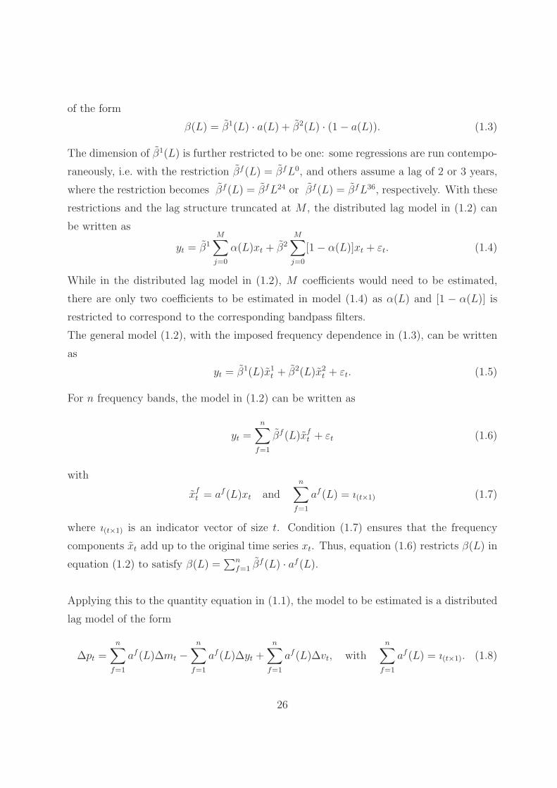
of the form

β(L) = β1(L) · a(L) + β2(L) · (1− a(L)). (1.3)

The dimension of β1(L) is further restricted to be one: some regressions are run contempo-

raneously, i.e. with the restriction βf (L) = βfL0, and others assume a lag of 2 or 3 years,

where the restriction becomes βf (L) = βfL24 or βf (L) = βfL36, respectively. With these

restrictions and the lag structure truncated at M , the distributed lag model in (1.2) can

be written as

yt = β1

M∑j=0

α(L)xt + β2

M∑j=0

[1− α(L)]xt + εt. (1.4)

While in the distributed lag model in (1.2), M coefficients would need to be estimated,

there are only two coefficients to be estimated in model (1.4) as α(L) and [1 − α(L)] is

restricted to correspond to the corresponding bandpass filters.

The general model (1.2), with the imposed frequency dependence in (1.3), can be written

as

yt = β1(L)x1t + β2(L)x2

t + εt. (1.5)

For n frequency bands, the model in (1.2) can be written as

yt =n∑

f=1

βf (L)xft + εt (1.6)

with

xft = af (L)xt and

n∑f=1

af (L) = ı(t×1) (1.7)

where ı(t×1) is an indicator vector of size t. Condition (1.7) ensures that the frequency

components xt add up to the original time series xt. Thus, equation (1.6) restricts β(L) in

equation (1.2) to satisfy β(L) =∑n

f=1 βf (L) · af (L).

Applying this to the quantity equation in (1.1), the model to be estimated is a distributed

lag model of the form

Δpt =n∑

f=1

af (L)Δmt −n∑

f=1

af (L)Δyt +n∑

f=1

af (L)Δvt, withn∑

f=1

af (L) = ı(t×1). (1.8)

26

Again for notational ease, define xft ≡ af (L)xt and restrict

∑nf=1 x

ft = xt so that the

frequency components add up to the original variables for xt = [ Δmt Δyt Δit ]. The

model to be estimated is then

Δpt =n∑

f=1

βfm(L)Δmf

t −n∑

f=1

βfy (L)Δyft +

n∑f=1

Δβfv (L)Δift + εt. (1.9)

The strict one-for-one relation between money and inflation as postulated by the quan-

tity equation would be straightforward to test: it would require that the bandpass filter

weights of all leads and lags, multiplied by their respective frequency dependent coefficient

estimate, would add up to zero; and the contemporaneous to unity. However, since the

interest rate is probably an imprecise proxy for velocity, we cannot expect to find the uni-

tary relationship of the quantity equation.

This model comprises several nice features: First, there is no loss of degrees of freedom (as

in band spectral regressions) because the dependent variable is unfiltered.8 Second, it is

very general and nests models such as the two-pillar Phillips curve. While the Phillips curve

literature suggests a positive impact of output growth on inflation, the quantity equation

postulates a negative correlation. In this model, each variable is allowed to impact head-

line inflation in a frequency dependent fashion, so it can take account of both relationships.

There are two major differences between equation (1.9) and the models typically applied

within the two-pillar Phillips curve framework: the output (gap) and the treatment of

velocity. The literature of the two-pillar Phillips curve follows the New Keynesian liter-

ature in adding a measure of the output gap to the empirical model in equation (1.8).9

Assenmacher-Wesche and Gerlach (2008b), for example, set up a model of headline infla-

tion that explains inflation at low frequency with the quantity equation variables and at

high frequency, inflation is driven by the output gap. The estimation results of such a

8Since the dependent variable is unfiltered, there is no loss in degrees of freedom stemming from filtering.See also Assenmacher-Wesche and Gerlach (2008b) on this issue. If the frequency components are thoughtto be estimated with a measurement error, then a classical errors-in-variables problem could arise. Inthis case, an attenuation bias would tilt the coefficients towards zero. Therefore, the estimates could beinterpreted as conservative.

9See e.g. Gerlach (2003), Gerlach-Kristen (2007), Assenmacher-Wesche and Gerlach (2007a).

27

model require special attention when the band spectral techniques along the lines of Engle

(1974) are applied. A measure of potential output can be thought of as lowpass filtered

output cLF (L)yt. Hence, the output gap is the corresponding highpass filtered output

(1 − L)cLF (L)yt. Then, when the estimation is run for low frequencies, what remains is

the portion of the output gap that corresponds to low frequencies only. If the output gap

is thought to correspond to business cycle fluctuations, then there should be no long-run

fluctuations in the output gap per definition, and the output gap filtered with a lowpass

filter should be a constant. Hence, in a low-frequency regression, the output gap should be

expected not to explain inflation when a constant is included. Figure 1.7 illustrates this

issue. It shows the lowpass filtered output gap (dark solid line) and the lowpass filtered

output growth (red dashed line). The output gap is supposed to explain high-frequency

movements in inflation, and output growth should drive inflation in the long run. However,

the graph shows that the lowpass filtered output gap is almost constant. Equation (1.8)

Figure 1.7: Lowpass-Filtered Output Gap and Output Growth

60 70 80 90 00 10−2

−1.5

−1

−0.5

0

0.5

1

1.5cLF(L)(1−cHP(L))y

t

cLF(L)(1−L)yt

allows to add different frequency components of output growth as explanatory variables.

Since the output gap is nothing but output growth at certain frequencies, it allows to

precisely measure the impact of the output gap, alongside with low-frequency movements

of real growth, i.e. potential output, on inflation.

The second issue that deserves attention is the treatment of velocity in equation (1.8).

28

Velocity is not directly observable. It is typically thought that money demand changes

with the interest rate, as interest rates determine the opportunity costs of holding money.

To account for shifts in money demand, money supply must be adjusted because such

demand-induced changes should not affect prices but rather cause a change in velocity.

Reynard (2006, 2007) therefore suggests adjusting money growth with some measure of

velocity. This adjustment comes down to estimating interest rate elasticity of money

demand in a first step. The corrected money growth rate is then used to empirically test

whether money contains information over inflation at higher frequencies. In particular,

Reynard (2006, 2007) estimates interest rate elasticity of money demand in a first step

from

vt ≡ mt − pt − yt = c+ ε · ln i10yt . (1.10)

Then, he runs regressions of the form

Δpt = c+ α1μt + α2μt−4 + α3μt−8 + ut (1.11)

where

μt = Δmt −Δy∗t + εΔi∗t (1.12)

with ∗ denoting a HP-filtered variable, so that Δy∗t is the potential growth rate, or the

long-run growth rate, and i∗t denotes some sort of equilibrium interest rate. So money

growth in excess of potential output growth is adjusted by equilibrium velocity. The goal

is to see whether money can explain inflation in the short term after imposing long-term

restrictions.

The regression equation (1.20), skipping the lagged regressors, can be thus written as

Δpt = c+ α1Δmt − α1Δy∗t + α1εΔi∗t + u1t (1.13)

Suppose the HP-filter is a good approximation to a low-pass filter, and note that a covari-

ance stationary variable can be decomposed into its frequency components. Then, equation

(1.20) can be written as

Δplft +Δphft = c+ α1Δmlft − α1Δylft + α1εΔilft + α1Δmhf

t + u1t . (1.14)

29

Since εΔilft is an estimate of the change in low-frequency velocity, the three low-frequency

terms are an estimate of low-frequency inflation. Thus, these three terms should be able to

explain the low-frequency inflation term well. What is left, then, to be explained is high-

frequency fluctuations in prices. The only high-frequency variable on the right-hand-side

left to explain short-term inflation is money growth. The following empirical estimations

are less restrictive. They allow all variables to explain inflation at all frequencies as all

frequency bands are included for each variable.

6 Regression Analysis of Money and Inflation

What matters for policy is the headline inflation rate rather than some frequency com-

ponent of it. Therefore, this section runs regressions on the unfiltered month-on-month

inflation rate. There are three main questions to answer: First, this section aims to find

the frequency band that is most important for the relation between money and inflation.

In particular, the question is whether money at business cycle frequencies contains infor-

mation over headline inflation. Second, the regression analysis tries to identify whether

there have been changes in the relationship between the two variables over time. Finally,

the model allows to test for the two-pillar Phillips curve and controls for changes in velocity.

6 .1 Frequency Dependence in the Relationship

The general model to be estimated, given in equation (1.9), does not restrict the frequency

components of the different variables to only contemporaneously affect headline inflation.

As a first step, however, the coefficients to be estimated, i.e. βfi (L) are restricted to be

contemporaneous only, so the restriction βfi (L) = βf

i L0 is imposed on equation (1.9). In a

second step, regressions are run for lagged money as the graphical analysis suggests that

there may be certain time shifts in the correlations.

A bandpass filter extracts the frequency components of a time series by computing a mov-

ing average with weights consisting of cosin terms. A bandpass filter has a phase shift of

30

zero, so the frequency component at time t corresponds to the time series’ observation at

time t. Hence, equation (1.8) can be considered as contemporaneous. As mentioned above,

however, empirical approximations to the optimal filter may exhibit certain phase shifts.

Moreover, a one-sided filter allows some interpretation with respect to the direction of the

correlation. Therefore, regressions are run separately for two-sided and one-sided filters.

Table 1.3: Regression Results

Dependent Variable: πt

Model two-sidedFilter

one-sidedFilter

Moneylagged by 2

years

Moneylagged by 3

years

m(0−1.5y)t -0.020 -0.009 -0.009 0.003

m(1.5−3y)t -0.138 -0.210 -0.076 -0.134

m(3−5y)t -0.123 -0.488 0.499 0.708∗

m(5−8y)t 0.180 0.194 0.903∗∗ 0.029

m(8−∞)t 0.439∗∗∗ 0.823∗∗∗ 0.887∗∗∗ 0.712∗∗∗

y(0−1.5y)t 0.007 0.011∗ 0.012∗∗ 0.013∗∗

y(1.5−3y)t -0.030 0.133 0.134∗ 0.057

y(3−5y)t -0.225∗ -0.022 0.063 0.048

y(5−8y)t -0.577∗∗∗ -0.524∗∗ -0.334∗ -0.166

y(8−∞)t -0.644∗∗∗ -0.596∗∗∗ -0.471∗∗∗ -0.412

i(0−1.5y)t 0.009 -0.029 -0.025 -0.028

i(1.5−3y)t 0.037 -0.175 -0.028 -0.062

i(3−5y)t 0.793∗ 0.607 0.972∗∗ 0.866∗∗

i(5−8y)t 1.076∗∗∗ 2.137∗∗∗ 1.171∗∗ 1.589∗∗

i(8−∞)t 1.670∗∗∗ 2.484∗∗∗ 2.342∗∗∗ 2.411∗∗∗

c -0.059 0.553∗∗ 0.390∗ 0.467Adjusted R2 0.3128 0.2441 0.2821 0.2544Number of Obs 576 576 563 551Durbin-Watson 1.3506 1.2536 1.3029 1.2394QLR statistic 93∗∗∗ 135∗∗∗ 91∗∗∗ 145∗∗∗

Breakpoint 1981/09 1981/09 1983/03 1981/09

These estimations are run for the sample from 1960/01 to 2007/12. Significance levels reported refer to

Newey West standard errors (12 lags). ∗∗∗, ∗∗, ∗ denote significance at the 1, 5, and 10% levels. The tilde

above each variable indicates that it is a frequency component of the time series. The superscript within the

parenthesis indicates the time correspondence of the frequency band.

31

Contemporaneous Regressions

Each of the three explanatory variables enters the regressions in the form of five frequency

components which reflect fluctuations of less than 1.5 years, 1.5 to 3 years, 3 to 5 years

5 to 8 years and more than 8 years. In line with the quantity theory, we would expect

a positive impact of money and a negative impact of output on inflation. On the other

hand, the Phillips curve relationship would call for a positive impact of the output gap

on inflation. If the interest rate is a good proxy for velocity, then theory would suggest a

positive coefficient.

Table 1.3 reports the regression results. The significance levels reported refer to Newey

West standard errors allowing for 12 lags. The sample spans from 1960 to the end of 2007.

However, as mentioned above, the frequency components are computed using the entire

sample of each individual variable. In the first column, the frequency components are

computed using the two-sided filter as in the graphical analysis. It suggests that money

is important for inflation only in the long run or at frequencies that correspond to more

than 8 years. Output has a positive sign only at the highest frequencies corresponding

to seasonality patterns, and it is very small. At business cycle frequencies, it is negative

but not statistically different from zero. At lower frequencies, the relation postulated by

the quantity equation is found.10 The coefficient estimates on the interest rate confirm

Reynard (2006, 2007) who suggested that there needs to be some sort of adjustment for

equilibrium velocity. In a regime of lower interest rates, velocity is lower and hence the

same money growth rate is associated with lower inflation rates. The fact that the low-

frequency components of the interest rate are highly significant is evidence that interest

rates at low frequencies can capture shifts in equilibrium velocity quite well. Interestingly,

none of the variables is capable of explaining inflation at high frequencies corresponding

to less than three years.

10The negative relation between inflation and output reminds of the fact that it is only money growthin excess of output growth that is typically thought to cause inflation. Regression results using thefrequency components of excess money to explain inflation turn out to be weaker, however. The obviousreason for this is that, as shown below, money performs best when lagged by 2 to 3 years, whereas outputshould enter the regression contemporaneously.

32

Two-sided filter regressions may capture feedback effects from the inflation rate to the

money growth rate. Therefore, the second column of Table 1.3 reports the estimates pro-

duced from one-sided filtering. Money enters significantly only at the lowest frequency,

but the size of the coefficient almost doubles. Output now enters significantly positive at

the highest frequency which suggests a similar seasonality pattern of output growth and

inflation. Moreover, the coefficient at 1.5 to 3 years has reached positive territory but

remains very small and insignificantly different from zero. Quantitatively, money becomes

more important at low frequencies when a one sided filter is used. This may indicate that

money leads inflation.

As Nelson (2003) notes, many studies fail to find the relationship by restricting it to be

contemporaneous. Therefore, the next section allows for a lag. The lagged regressions

also use a one-sided filter. This choice was taken not only because results are better in-

terpretable from a one-sided filter, but also because the one-sided frequency components

were found to even outperform their two-sided counterparts, as the comparison of the two

first columns in Table 1.3 suggest. A symmetric two-sided filter does not cause a phase

shift of the filtered series. The computation of the frequency components in this study,

however, sacrifices the symmetry of the filter in favor of the precision of the estimates. To

obtain as accurate estimates as possible, the filter employed uses all information available

at all times. Thus, in the first half of the sample the frequency components contain a

forward bias as the frequency component is estimated only from subsequent observations.

Likewise, the end of the sample exhibits a backward looking bias. In the spirit of precision,

the one-sided filter is constructed to incorporate all information available at all times. But,

because it is a one-sided filter, the information is restricted to the past. As a consequence,

the frequency components contain relatively more information of the past towards the end

of the sample. The graphs in Figure 1.6 give evidence that money lead inflation by more

(about 3 years) in the most recent subsample than in the early years (about 2 years). Note

that this should not be the product of filtering as both variables were filtered the same

way so that the phase shifts balance. Because a one-sided filter induces an increasing the

phase shift, it may perform better in the regression analysis.

33

Allowing for a Lag

As mentioned above, the general model given in equation (1.9) is a distributed-lag model

of the frequency components. However, serious multicollinearity issues arise with several

lags of each frequency component entering the regression. This is true especially for low-

frequency components as these are highly autocorrelated. The graphical analysis above

suggests that money growth leads inflation by 2 to 3 years. In line with these findings, the

regression is run with the frequency components of money entering with a lag of 2 and 3

years.11 Column 3 and 4 of Table 1.3 report the respective results. With a lag of two years,

money becomes highly significant at the lower business-cycle frequencies corresponding to

5 to 8 years. With a lag of three years, the explanatory power of money shifts even to

those components that correspond to fluctuations of 3 to 5 year length. Thus, the patterns

visible in the graphs can indeed be confirmed by regressions on headline inflation. This is

evidence that money matters for inflation not only in the long run, but also at frequencies

well within the business cycle.

With money lagged by two years, the output fluctuations of 1.5 to 3 years’ duration impact

on inflation. Thus, this is evidence for the Phillips curve relationship. With a lag of three

years, the explanatory power of output growth largely disappears. In general, the evidence

for a Phillips curve type relation is rather weak. Possibly, the Phillips-curve effect is cap-

tured by the interest rate, as a high interest rate often goes hand-in-hand with a positive

output gap, which puts upward pressure on prices.Neighboring frequency components of a

variable are uncorrelated by definition. Correlation could only arise due to leakage, which

is very small as shown in Figure 1.9 in appendix B . However, the frequency components

across variables may be correlated within certain frequency bands. Such multicollinearity

issues may make it difficult to clearly disentangle the effects of each variable from the oth-

ers’. Table 1.4 therefore shows the correlations among the variables at different frequencies.

Frequency components of the interest rate do exhibit quite large correlations with other

variables. It is for example highly negatively correlated with money at frequencies between

11It may not be fair to only lag money. Moreover, lagging money restricts the coefficients∑n

f=1 βfm(L)

in (1.9) in an arbitrary way. However, as mentioned in the graphical analysis, the correlation betweenoutput and inflation seems to be contemporaneous. Moreover, regressions show a clear deterioration ofthe explanatory power of output when it is lagged.

34

Table 1.4: Correlation of Frequency Bands

Sample: 1960/01 to 2007/12

Frequency band correspondence0 to 1.5 1.5 to 3 3 to 5 5 to 8 8 to ∞

m and y -0.1833 -0.1213 0.1907 0.2105 -0.0248m and i -0.0094 -0.2215 -0.2444 -0.6044 0.1509y and i 0.0166 0.6240 0.7381 0.3615 0.2985

5 and 8 years. Moreover, its correlation with output growth is very large at business cycle

frequencies. This may explain why it is difficult to find the positive effect of output at

those frequencies.12

To conclude, the regression results suggest that money is most important for inflation in

the long run, and there is only limited explanatory power in fluctuations corresponding to

the business cycle. However, if the comovement between money and inflation, e.g. due to

changes in velocity, shift between frequency bands over time, or if the lag structure evolves,

then the regressions above are not able to capture such changes.

6 .2 Time-Variance in the Relationship

The graphs in Section 4 indicate that the relationship between money and inflation changed

with the beginning of the Volcker era around 1980. To test this, breakpoint tests are run

on the regressions above. As a second step, a dummy variable is included to allow for a

different coefficient during that time.

Andrews (2003)

Breakpoint Tests

Chow’s (1960) breakpoint test provides a means to test whether a coefficient has changed

at a given point in time. The Chow breakpoint test is based on a comparison of the sum of

12When the interest rate enters the regression as an unfiltered measure to avoid such multicollinearity,the results for output remain almost unchanged while the goodness of fit of the regression deterioratesconsiderably.

35

squared residuals obtained by fitting a single equation to the entire sample with the sum of

squared residuals obtained when separate equations are fit to each subsample of the data.

The F-statistic

ξW =(u′u− u′

1u1 − u′2u2)/k

u′1u1 + u′

2u2)/(T − 2k)(1.15)

is based on the comparison of the restricted and the unrestricted sum of squared residuals,

where u′u is the restricted sum of squared residuals and u′iui is the sum of squared residuals

of each subsample. k is the total number of parameters in the equation. The F-statistic

can be extended to more than one breakpoint. However, the date of the breakpoint must

be known in order to apply the Chow test. With unknown breakpoint, the Chow statistic

can be run for a large number of possible breakpoints. With τ denoting the fraction of the

sample, the Quandt likelihood ratio (QLR) statistic

ξQ = maxτ1≤τ≤τ2

ξW (τ) (1.16)

gives the largest value of the Chow statistics running from τ1 to τ2. The breakpoint lies

somewhere between the end of the 1970s and the mid 1990s. This information should be

incorporated to maximize power of the test. In order not to be too restrictive, only the

dates between 1975 and 2000 are included in the test. The respective fractions of the sam-

ple are τ1 = 0.31 and τ2 = 0.78. ξQ no longer follows a χ2 statistic. The critical values are

originally tabulated in Andrews and Ploberger (1994) and revised in Andrews (2003). The

1%, 5%, and 10%-critical values for the QLR statistic, with k = 16, are 40.87, 35.15, and

32.36, respectively. The two rows at the bottom of Table 1.3 indicate the results of such a

breakpoint test. The statistics clearly exceed the respective critical values, indicating that

there was a structural break somewhere at the beginning of the 1980s.

Inclusion of Dummy Variables

The graphical analysis above suggests that there is a close relation between money and

inflation at business cycle frequencies, but that this relation broke down during the Volcker

era. Whether it appeared again during the past 20 years is not clear from the graphs. This

would mean that there was a temporary structural break during approximately one and a

36

half decades. In order to shed light on this, dummy variables are added to the regressions

above.

In a first step, the different frequency components of money are interacted with a dummy

variable for the time interval between 1980 and 1995 and added to the regression. Table 1.5

gives the results in the first column. The coefficient on the frequency band corresponding

to 3 to 5 years increases and becomes significant.13 Moreover, the coefficient on the lower

business cycle frequencies increases further. Hence, money affected inflation differently

during and after the disinflation period. And, controlling for this period suggests a very

strong comovement at business cycle frequencies. There is only very weak evidence that

the relationship had moved to the higher frequencies, however. The respective coefficient

turns from negative to positive, but it remains statistically insignificantly different from

zero.

In a second step, another dummy is interacted with money to allow the relationship to be

different since 1995. The results are depicted in the second column of Table 1.5. The 3 to

5 year frequency component of money remains significant. But when interacted with the

dummies for both later subsamples, its size is strongly reduced. While the relationship is

even reversed during the Volcker era and the subsequent years, it is approximately halved

since 1995. It seems that part of this long-run correlation has moved to a higher frequency

band. In the recent one and a half decades, the most important frequency band seems to

be the one corresponding to 5 to 8 years. Moreover, there is the indication that the long

term relation between money and inflation has been significantly smaller since 1995. This

is in line with Nelson (2003) who argues that “a protracted fall in nominal interest rates,

associated with the aftermath of a disinflation, reduces the cost of holding real balances

and so generates data characterized by higher money growth, slower velocity growth and

unchanged inflation”.

Finally, the last column of Table 1.5 imposes the assumption that the relationship changed

with the Volcker era and remained stable since. This regression confirms that the comove-

13Note that when the sample is extended to June 2011, the inclusion of the dummy variable lets thefrequency component of money corresponding to 3 to 5 years become significant even at the 1% level.

37

Table 1.5: Dummy Regressions

Dependent Variable: πt

m(0−1.5y)t -0.003 0.034 0.032

m(1.5−3y)t -0.129 -0.241 -0.22

m(3−5y)t 0.676∗ 0.743∗ 0.794∗∗

m(5−8y)t 0.958∗ 0.636 0.804

m(8−∞)t 0.894∗∗∗ 0.779∗∗∗ 0.892∗∗∗

D1 · m(0−1.5y)t -0.020 -0.054 -

D1 · m(1.5−3y)t 0.205 0.323 -

D1 · m(3−5y)t -0.928 -0.858 -

D1 · m(5−8y)t -0.263 0.199 -

D1 · m(8−∞)t 0.062 -0.024 -

D2 · m(0−1.5y)t - -0.083 -

D2 · m(1.5−3y)t - 0.168 -

D2 · m(3−5y)t - -0.369 -

D2 · m(5−8y)t - 0.346 -

D2 · m(8−∞)t - -0.218∗∗∗ -

(D1 +D2) · m(0−1.5y)t - - -0.065

(D1 +D2) · m(1.5−3y)t - - 0.218

(D1 +D2) · m(3−5y)t - - -1.026∗

(D1 +D2) · m(5−8y)t - - -0.014

(D1 +D2) · m(8−∞)t - - -0.084

y(0−1.5y)t 0.011∗ 0.013∗∗ 0.013∗∗

y(1.5−3y)t 0.131 0.144 0.146∗

y(3−5y)t 0.048 0.026 0.018

y(5−8y)t -0.318∗ -0.404∗∗ -0.409∗∗

y(8−∞)t -0.418∗∗ -0.609∗∗∗ -0.575∗∗∗

i(0−1.5y)t -0.024 -0.030 -0.030

i(1.5−3y)t 0.027 -0.049 -0.056

i(3−5y)t 0.906∗∗ 1.034∗∗ 1.900∗∗

i(5−8y)t 0.937∗∗ 1.165∗∗∗ 0.961∗∗

i(8−∞)t 2.247∗∗∗ 2.363∗∗∗ 2.208∗∗∗

c 0.317 0.614∗∗∗ 0.491∗∗

Adjusted R2 0.2844 0.3101 0.2959Number of Obs 563 563 563Durbin-Watson 1.3185 1.3885 1.3470

These estimations are run for the sample from 1960/01 to 2007/12. Money is lagged by 2 years. The dummy variables D1

and D2 refer to the time intervals 1980 to 1994 and 1995 to 2007, respectively. Significance levels reported

refer to Newey West standard errors (12 lags). ∗∗∗, ∗∗, ∗ denote significance at the 1, 5, and 10% levels.

ment between money and inflation at frequencies corresponding to 3 to 5 years is limited to

the first part of the sample. It seems to persist only at the lower business cycle frequencies

38

and in the long run.

To sum up, this method is partially able to identify the change in the comovements over

time as suggested by the graphical analysis in Section 4 . However, the relationship at

frequencies corresponding to 3 to 5 years is strongest in the early subsample ending 1979,

it disappeared during the Volcker era and might have come back at a weaker level. At

the lowest frequency, a very similar pattern reveals: the relation between money and infla-

tion is smaller in the latest subsample starting 1995. The results of the empirical analysis

shows clearly that the relationship between money and inflation is not stable over time. It

moves both with respect to frequencies as well as to the lag structure. A linear model such

as a vector autoregression imposes a constant lag structure over time. The estimates will

therefore be biased towards zero if the assumption of time stability is violated. In addition,

the analysis shows that to identify the comovement between money and inflation, different

frequency bands should be taken into account.

7 Conclusion

Money and inflation are most often shown to correlate only in the “long run”. But there

is very little precision as to the actual timing of the comovement. From a policy per-

spective, however, it is important to have a better understanding of the timing of such a

comovement. Therefore, this paper studies the correlation between money and inflation

at different frequency bands. Money and inflation are found to correlate strongest at low

frequencies, i.e. at cycles of more than 8 years’ length. In the 1980s and early 1990s, when

the correlation between money and prices is typically found to break down, graphical anal-

ysis suggests that the correlation might have shifted into higher frequency bands. Yet, the

regression analysis is unable to replicate this result. But when controlling for that period,

the regression results show a strong comovement between money and inflation at frequen-

cies that correspond to the business cycle, i.e. of 3 to 8 years’ fluctuations. Moreover, the

results suggest that, after a break during the Volcker era and the subsequent years, the

correlation returned in the mid 1990s. The more recent relationship is slightly weaker and

more pronounced at lower frequencies, however. Since the mid 1990s, however, the corre-

39

lation concentrates at higher frequencies that correspond to 5 to 8 years. These results not

only support the evidence that there is indeed a comovement between monetary aggregates

and inflation, but that this comovement changes over time with respect to both the lead-

lag structure and with respect to the relevant frequencies. While linear models may suffer

from biased estimates due to the absence of time stability, spectral techniques as applied

in this study seem to be a suitable instrument to further investigate this relationship.

40

A Some Properties of Bandpass Filters

A bandpass filter is a lag operator that attributes certain weights to leads and lags of a

variable. The low-pass filter passes all movements in a variable that are attributable to

frequencies below a chosen threshold, ωa. It can be shown that the optimal low-pass filter

a(L) =∞∑

j=−∞ajL

j (1.17)

where L denotes the lag operator, has weights that take the form

aj = (2π)−1 1

ijeiωj|ωa

−ωa =

{1jπsin(ωaj) for j �= 0

ωa

πfor j = 0

. (1.18)

Equivalently, the filter (1 − a(L)) is a high-pass filter passing all frequencies larger than

ωa. The low-frequency and high-frequency components a(L)xt and (1 − a(L))xt of some

variable xt are uncorrelated by construction. Moreover, filters are additive in their gains,

so the low-frequency and high-frequency components a(L)xt and (1 − a(L))xt add up to

the original time series xt. Suppose a(L) is a low-pass filter that passes on frequencies

lower or equal to ωa. Let b(L) be another low-pass filter that passes on frequencies up to

ωb, where ωa < ωb. Then, the bandpass filter c(L) = a(L) − b(L) passes all frequencies

ωc that lie between the lower and the upper threshold, so ωa < ωc < ωβ. Thus, using

bandpass filters, we can decompose a time series into its different frequency components.

B Bandpass Filter Gain

There is always the issue of end-of-sample accuracy of filters. The bandpass filter applied

in this study uses all the information available for each data point. So as an approximation

to the optimal filter in (1.17), the filter weights are truncated at the start and at the end

of the sample. Thus, at the beginning of the sample, the filter is mainly forward-looking.

Towards the end of the sample, the filter is backward-looking. Likewise, the gain of the

filter varies among observations t. Figure 1.8 shows the gain of the bandpass filter. In

the left panel, the gain is plotted for the filter at each observation t. In the right panel,

41

the gains of the first and last 5% of observations are dropped. This shows that the filter

provides a reasonable approximation to the ideal filter after dropping approximately 5%

of observations at both ends.

Figure 1.8: The Gain of the BP-Filter at Each Observation

0 0.065 0.105 0.175 0.349 0.5240

0.2

0.4

0.6

0.8

1

1.2

1.4

Frequency ω

Gai

n

0 0.065 0.105 0.175 0.349 0.5240

0.2

0.4

0.6

0.8

1

1.2

1.4

Frequency ω

Gai

n

The entire sample of each variable is used to compute the frequency components. As

regression start in 1960, and inflation, industrial production, and interest rates are available

way back, it is only the frequency components of money that might suffer from poor end-

of-sample properties of the filter. The data is collected through June 2011, regressions are

run only up to the end of 2007. So at the end of the sample, 42 observations are dropped.

Despite the fact that there are most likely enough data dropped at both ends of the sample,

the impact of dropping data can easily be analyzed empirically. I computed different

frequency components for inflation, applying the bandpass filter to 11 different samples:

the full sample, cut 1 year at each end, cut 2 years at each end, etc. The following results

obtain: At high frequencies corresponding to less than 4 years, as the filtered series are

almost identical. Hence, there is no reason to cut any data. The deviations are still minor

for frequency components corresponding to 4 to 8 years. Even for those corresponding to 8

to 15 years, the differences are relatively small. However, for the very low frequencies, there

are shifts in the trend that are quite large. This is true even when the data is detrended

prior to filtering. And it is also true whether detrending is undertaken in the time or in the

spectral domain, as Corbae et al. (1997) suggest. To conclude, end-of-sample properties

are certainly not an issue for frequencies corresponding to cycles of less than 15 years.

42

For the very low frequency components, uncertainty about the precision of the frequency

component is larger. This is true not only with respect to poor end-of-sample properties

of the filter, but also with respect to prior manipulation of the data with respect to trends.

I do the best I can by letting the filter use all the information available at each point in

time.

Another empirical issue related to the gain is leakage. Since the filter in an empirical appli-

cation is always an approximation to the ideal filter, it is imprecise. The less observations,

the larger is the leakage, which refers to the near-by frequencies outside of the particular

passband that are partially passed by the filter due to its imprecision. Figure 1.9 shows the

gain of the bandpass filter for the frequency bands relevant for the empirical section of this

paper. The vertical dotted lines indicate the exact frequencies ω of the thresholds between

the frequency bands. For example, ω = 0.105 denotes the period 2 · π/ω = 60. Since we

have monthly data, this corresponds to 5 years. So when the gain of a certain passband

crosses the corresponding frequency, it means that bits outside of the passband are passed

by the filter. To compute these gains, a sample size of 564 observations is used, which

corresponds to monthly data of 47 years, i.e. from 1960 to 2007. The Figure clearly shows

that there is some leakage when the bandpass filters are constructed without dropping

intermediate frequencies. However, a problem for the present analysis arises only if leakage

leads to multicollinearity, such that the contributions of the separate frequency bands can

no longer be clearly disentangled. Looking at the correlation matrix of the frequency bands

confirms for each variable that the correlations are rather small. Hence, leakage can be

ignored.

C End-of-Sample Properties of Bandpass Filter

In theory, the ideal bandpass filter is a symmetric weighted average of an infinite number of

leads and lags. In practical applications, there are essentially two ways to approximate the

ideal filter: First, a symmetric filter with relatively few leads and lags can be computed.

Second, an asymmetric filter can be constructed that uses all data points available at each

point in time. The former method requires to drop data at both the beginning and at the

end of the sample. The latter method potentially induces a phase shift. This paper uses

the second method. The entire sample of each variable is used to compute the frequency

43

Figure 1.9: Leakage of the Bandpass Filter

0 0.035 0.065 0.105 0.175 0.3490

0.2

0.4

0.6

0.8

1

Gai

n

ω

1.5−3 years 3−5 years 5−8 years 8−15 years 15−∞ years

components. Hence, even if the final regression is run starting only in 1995, the frequency

components of M2 use data back to 1959. However, the filter might still suffer from poor

end-of-sample properties, especially in those samples starting in 1960. Hence, it may be

necessary to cut some observations at least at the end of the sample. In order to find out

how much needs to be cut, different frequency components for inflation were computed,

applying the bandpass filter to 11 different samples: the full sample, 1 year cut at each end,

2 years cut at each end, etc. The following results obtain: At high frequencies (0-4 years),

there is no reason to cut data, as the filtered series are almost identical. The deviations

are still minor for frequency components of 4-8 years, and even for those corresponding to

8-15 years, the differences are relatively small. For the very low frequencies, there are shifts

in the trend that are quite large. This is true even when the data is detrended prior to

bandpass filtering (this is true for detrending both in the time and in the spectral domain).

D Velocity Adjustment of Money

In a first step, Reynard (2006, 2007) estimates interest rate elasticity of money demand

from

vt ≡ mt − pt − yt = c+ ε · ln i10yt . (1.19)

44

Then, he runs regressions of the form

Δpt = c+ α1μt + α2μt−4 + α3μt−8 + ut (1.20)

where

μt = Δmt −Δy∗t + εΔi∗t (1.21)

with ∗ denoting a HP-filtered variable, so that Δy∗t is the potential growth rate, or the

long-run growth rate, and i∗t denotes some sort of equilibrium interest rate. So money

growth in excess of potential output growth is adjusted by equilibrium velocity. The goal

is to see whether money can explain inflation in the short term after imposing long-term

restrictions.

The regression equation (1.20), skipping the lagged regressors, can be thus written as

Δpt = c+ α1Δmt − α1Δy∗t + α1εΔi∗t + u1t (1.22)

Suppose the HP-filter is a good approximation to a low-pass filter, and note that a covari-

ance stationary variable can be decomposed into its frequency components. Then, equation

(1.20) can be written as

Δplft +Δphft = c+ α1Δmlft − α1Δylft + α1εΔilft + α1Δmhf

t + u1t . (1.23)

Since εΔilft is an estimate of the change in low-frequency velocity, the three low-frequency

terms are an estimate of low-frequency inflation. Thus, these three terms should be able to

explain the low-frequency inflation term well. What is left, then, to be explained is high-

frequency fluctuations in prices. The only high-frequency variable on the right-hand-side,

however, is money growth. Surely, high-frequency fluctuations in money growth are not

what we would expect to explain short-run fluctuations in inflation.

45

Chapter 2

Liquidity Effects of Quantitative

Easing on Long-Term Interest Rates

Abstract

This paper argues that the expansion in reserves following recent quantitative easing pro-

grams of the Federal Reserve may have affected long-term interest rates through liquidity

effects. The data lends some support for liquidity effects, in that reserves were negatively

correlated with long-term yields at the zero lower bound. Estimates suggest that between

January 2009 and 2011, 10-year US Treasury yields fell 46-85 basis points as a result of

liquidity effects. The liquidity effect is separate from the portfolio balance effect of the

change in the public supply of Treasury bonds, which is estimated to have reduced yields

by another 20 basis points during that period.

47

1 Introduction

An increase in the money supply is usually expected to reduce short-term interest rates.

This phenomenon, known as the liquidity effect, finds empirical support in the literature.

It is commonly held that when short-term interest rates reach the zero lower bound (ZLB),

the liquidity effect disappears. This is because the short-term liquid assets typically bought

in open market operations (OMO) form a perfect substitute for money when short-term

interest rates are at zero. However, banks also demand and hold long-term assets with

strictly positive yields. OMOs in long-term bonds could hence still have a liquidity effect.

The increase in zero-yielding reserves associated with the purchases of longer term bonds in

OMOs at the ZLB, induces banks to search for a higher return on their assets. They hence

raise their demand for positive yielding medium to longer-term assets, such as government

bonds. The higher demand for these assets, in turn, reduces their yield. In this way, an

increase in reserves should be related to lower long-term yields at the ZLB.

That the large scale asset purchases conducted by the Federal Reserve at the ZLB may

have been transmitted to yields through such liquidity effects has been overlooked. Chart

2.1 shows how non-borrowed reserves held with the Federal Reserve, and long-term Trea-

sury yields, moved in the same overall direction during the recent ZLB period. There

could be many reasons for these variables to have been correlated during that period. One

candidate is that the relationship is partly causal.

Instead of focusing on the effect of reserves, the currently very active literature has focussed

on the effect of the assets purchased in these operations. Thus, the expansion in reserves

during the past years came about partly through outright purchases of Treasury bonds.

When the central bank buys a government bond, it augments the asset side of its balance

sheet with this bond, and augments the liability side with the corresponding amount of

reserves. The liquidity effect is the impact of an expansion of the central bank’s liabili-

ties on bond yields, irrespective of the type of asset the central bank buys. The previous

literature argues that the change on the asset side of the balance sheet, i.e. the outright

purchase of a specific asset, such as a specific maturity government bond, constitutes the

main channel through which quantitative easing influences the yield on this bond, as the

48

quantity of the purchased bond in the market changes.

In this paper, we lay out the argument for why liquidity effects may have been at work, and

take a first look at the data to offer some initial empirical support for the hypothesis that

liquidity effects constitute an additional and potentially important transmission channel,

increasing the overall impact of the asset purchases on long-term rates. Specifically, we

add reserves to a standard regression specification for the 10-year Treasury yield used for

testing for supply effects. We allow the effect of reserves on yields to differ between the

present ZLB period and the pre-ZLB period in this regression.

We find that (i) the realized yield on the 10-year Treasury bond has been lower during the

recent ZLB period than what the standard regression used for testing for supply effects

predicts and (ii) adding non-borrowed reserves in percent of GDP to the regression results

in a significantly negative effect of reserves on yields at the ZLB. The estimated correlation

between reserves and yields suggest that yields were 46-85 basis points lower during the

ZLB period due to liquidity effects of the monetary expansion. This liquidity effect is in

addition to the supply effect, meaning that the overall impact of the asset purchases at the

ZLB was larger.

The next section offers some theoretical considerations regarding how central bank asset

purchases might affect the yield of bonds through liquidity effects as well as supply effects.

The empirical investigation of liquidity effects is set up in the subsequent section. The

final section concludes.

2 How Do Central Bank Asset Purchases Affect In-

terest Rates?

How should we expect a change in commercial banks’ reserves held at the Fed to affect

long-term interest rates, and how important has the effect been during the ZLB period of

quantitative easing (QE) programs? To see this, consider three assets: reserves M with

49

zero yield, a short-term treasury bill A with yield rA, and a long-term treasury bond B

with yield rB.

The recent literature on the effects of QE on long-term yields have focused on the impact of

changes in the quantity B, i.e. Fed’s purchases of long-term bonds and government supply

of Treasuries, on rB, which is referred to as portfolio balance or supply effect, as well as on

the signaling effect which is not discussed here (see next Section). This approach is based

on portfolio balance models incorporating different assets with imperfect substitutability

through financial frictions. In these models, a change in the relative supply of A and B

affects their relative yield. Thus, in a portfolio balance model with market imperfections,

such as segmented markets and assumptions of preferred habitat, a central bank purchase

of an asset must increase the price of the asset in question, in order to make market par-

ticipants accept holding less of the respective asset.1 Hence, the yield of the asset falls.

Recent empirical research, such as Kuttner (2006), Gagnon et al. (2010), Greenwood and

Vayanos (2010), Hamilton and Wu (2010b), Neely (2010), and D’Amico and King (2011),

shows that central bank purchases of specific assets influence their yields through so-called

supply effects.

This so-called supply effect relates to the asset side of the central bank’s balance sheet.

The models do not incorporate the equivalent increase in the liabilities side of the balance

sheet, namely reserves. The effect of changes in reserves, or liquidity effect, has been ad-

dressed in frameworks that have modeled the private sector’s choice between reserves, M ,

and a short-term bond, A. In practice, the liquidity effect arises from the fact that the

portfolios of banks involved in OMOs include more reserves than before the sale of assets

to the central bank. A higher level of reserves is empirically found to be related to a fall in

short-term interest rates, in normal times. Specifically, the liquidity effect has been found

to reduce short-term interbank deposit rates such as the Federal funds rate in the US, and

short-term government bond yields; see for example Cochrane (1989), Gordon and Leeper

(1994), Christiano and Eichenbaum (1995), Christiano and Eichenbaum (1992a), Hamilton

(1997), Bernanke and Mihov (1998), Carpenter and Demiralp (2008), Thornton (2008a),

1Recent examples of preferred-habitat models include Hamilton and Wu (2010b) or Greenwood andVayanos (2010).

50

Hagedorn (2009), or Judson and Klee (2010). Liquidity effects have been modeled using

segmented market assumptions. Examples of such models are Grossman and Weiss (1983),

Christiano and Eichenbaum (1992b), Lucas (1990), or Dotsey and Ireland (1995). In line

with a cash-in-advance constraint, a central bank’s lump sum monetary injection cannot

immediately be used as transaction balances by the private agents receiving the injection.

It therefore pushes up the price of the alternative asset available to market participants.

In practice, the mechanisms in models of the liquidity effect are similar to the ones at work

in the portfolio balance approach. In fact, liquidity effects can be thought of as supply

effects of reserves. The only differences are the purpose of asset holdings, and the types

of frictions. Banks, holding more reserves after an OMO, seek to trade some of these ad-

ditional reserves for positive yielding assets. Given that the yield on reserves M is fixed

at zero, the higher demand for A and B should put upward pressure on the price of both

of these assets and thus reduce their yields, in contrast to the supply effect which only

pertains to the yields of the specific asset bought in the OMO or to its close substitutes.

Indeed, Cochrane (1989) finds that liquidity effects influence the entire yield curve. An

important difference between supply and liquidity effects is that while the former suggest

a long term link between the supply of an asset and its yield, liquidity effects suggest a

link between reserves and interest rates which is temporary. The reason is that an increase

in reserves will only affect yields as long as it is in excess of required reserves. But with

time, higher excess reserves transform into increased bank credits, which in turn reduce

excess reserves (turn excess reserves into required reserves). This is in line with the em-

pirical literature. For example, Christiano and Eichenbaum (1992a) and Christiano and

Eichenbaum (1995) find temporary liquidity effects in short rates lasting from one to 20

quarters.

Both the supply effect and the liquidity effect rely on imperfect asset substitutability and

should be addressed jointly in the same framework. This would allow for an evaluation of

the total effect of QE on long-term yields. Tobin (1958) has suggested a portfolio analysis

with money and bonds of different maturities. Andres et al. (2004) provided a theoretical

framework including these assets. To understand how the different effects of an OMO can

be combined, consider again the three assets M , A and B. A supply effect occurs when the

51

supply of B changes, for example when the government pays back some long-term debt.

In this case, the yield rB decreases. A liquidity effect occurs as a result of a change in the

supply of reserves M , for example through a ”helicopter drop” of reserves on banks. In

this case, the ”yield” of reserves compared to the yield of other assets has to change. With

zero or a low and fixed interest on reserves, this will put downward pressure on the yields

of both assets A and B.

In normal times, during an OMO, the central bank (CB) buys A with M , thus the supply

and the liquidity effect both put downward pressure on rA, and the liquidity effect puts

downward pressure on rB. Note that we isolate here the supply and liquidity effect from the

Fisher effect which can drive yields in the other direction. At the ZLB, when the CB buys

B with M, both the supply and liquidity effect put downward pressure on rB. The yield on

the short-term bill, rA, can be pushed down by the liquidity effect, if it is not already at

the ZLB. It is often argued that there cannot be liquidity effects at the ZLB, when A has a

zero yield like M . But the total supply of zero-yielding assets M and A increases relative

to B when the CB buys B in OMO, putting downward pressure on rB in addition to the

supply effect. Finally, note that in the case of the current maturity extension program

”Operation Twist II”, the CB buys B and sells A. In that case there is no liquidity effect

which would put downward pressure on both rA and rB, as the amount of reserves remain

constant. Supply effects put downward pressure on rB and upward pressure on rA.

3 An empirical assessment

As argued above, a central bank asset purchase directly from the market is transmitted

through at least three different channels, namely the supply effect, the liquidity effect

and through signalling. Signalling effects occur because a central bank asset purchase may

signal something about the central bank’s intentions for future monetary policy, and hence,

the future short term interest rate path. We hence need a research design which allow us

to distinguish these three effects. The following sections present how we approach these

issues conceptually and econometrically.

52

3 .1 Identifying liquidity effects

If market participants are informed about asset purchases by the central bank in advance -

as has been the case for all three recent large scale asset purchase programs (LSAP) - and

if market participants have perfect and complete information, and hence know the impact

of these purchases on yields through supply and liquidity effects, then this impact should

be discounted immediately at announcement. In contrast, there should be no effect on

yields when the transactions actually take place under these assumptions. A number of

studies estimating the supply effects of the Fed’s asset purchases have hence looked for an-

nouncement effects on yields, using event studies techniques. In order to identify portfolio

balance effects from signalling effects at announcement, such studies divide the long-term

Treasury yield into a term premium and the expected future short rates using econometric

term structure models. Supply effects affect the term premium whereas signalling effects

should only affect expected future short rates (see for example Bauer and Rudebusch (2011-

21) and the first part of the analysis in Gagnon et al. (2010). Neely (2010) is an exception).

The event study approach does not allow for an identification of liquidity effects. This is

because both liquidity and supply effects affect the term premium at the ZLB. Their indi-

vidual effects hence cannot be identified by simply investigating the reaction of the term

premium. There are other problems with the use of event studies in this context. One is

that the breakdown between the expected future short rates and the term premium turns

out to be very uncertain, and dependent on the type of term structure model estimated,

see for example Bauer and Rudebusch (2011-21). Another problem is that the assumption

of complete and perfect information of market participants, which is necessary for inter-

preting the effect of an announcement on yields as containing information about supply

and liquidity effects, might be too strong.

Instead, we take a different approach to identification and note that if market participants

do not have perfect and complete information, then there is room for some of the liquidity

and supply effects of planned transactions to materialize when the actual transactions take

place. Signalling effects, on the other hand, should only be present at announcement times.

In the time series dimension, what matters for the supply effect is the total supply of the

53

asset in question, i.e. the total supply of Treasury bonds available to the public. This

supply has been affected by the Fed’s purchases during the LSAP, but it has also - and to

an even higher degree - been affected by the Treasury’s net issuance of new bonds. For

this reason, the public supply of Treasuries has had a source of independent variation,

and its correlation with reserves is actually quite small. If there is an effect of reserves

on long-term treasury yields when controlling for the public supply of Treasuries, then it

should be possible to interpret this effect as a liquidity effect, as separate from a supply

effect.

3 .2 Methodology and Data

We take as a starting point the time series approach employed by Gagnon, Raskin, Remache

and Sack (2010) to assess supply effects in a regression of long-term treasury yields. We

add reserves to the regression in order to see if these help explain variation in long-term

yields at the ZLB. The effect of reserves is allowed to differ between the pre-ZLB and the

ZLB periods. The sample ranges from February 1990 to January 2011. The regressions

are carried out in weekly frequency, yielding 112 observations for the ZLB period and

1096 observations for the entire sample. The few explanatory variables for which data is in

lower frequency are linearly interpolated (see appendix for details). The baseline regression

equation takes the following form:

i(10y)t = α + β1 ·Dpre−ZLB

t Rt−1 + β2 ·DZLBt Rt−1 + β3D

ZLBt + δXt + ut. (2.1)

i(10y)t denotes the average daily yield on 10-year US Treasury bonds over the week following

t − 1.2 Rt−1 denotes the level of non-borrowed reserves held with the Fed at date t − 1,

in percent of GDP.3 Reserves are thus effectively lagged one week. Dpre−ZLBt and DZLB

t

are dummy variables for the pre-ZLB and the ZLB period, respectively. Xt contains the

control variables described below. We define the ZLB to start in mid December 2008, when

the Federal funds target rate was lowered to 0.25%. The interaction of reserves with these

2All control variables for which data is available on a daily basis enter in averages over the week followingt− 1.

3We use the percentage of GDP to make reserves comparable in specification to the specification of theTreasury supply, see below. It should be mentioned that the results obtained in this paper are not drivenby changes in GDP. When carrying out the regressions using nominal reserves, all results remain.

54

dummies allows the liquidity effect to differ between normal times and at the ZLB. The

level of the ZLB-dummy is included to capture a change in the interest rate level during

the ZLB period due to factors that cannot be fully accounted for by the explanatory vari-

ables.

The supply of Treasury securities to the public in percent of nominal GDP is included to

capture supply effects. Treasury supply is measured as the total supply minus the Fed’s

holdings of Treasury securities, as reported in the System Open Market Account (SOMA).

We include all maturities above one year in order to account for the transmission of changes

in the supply of Treasury bonds to other maturities through substitution effects.4 Since

changes in the maturity structure of the total supply could matter for the supply effect on

longer yields, we also control for the average maturity of Treasury bonds.5

The Federal funds target rate is included to account for the current interest rate level. Both

reserves and the long-term yields may have been driven by weakening economic conditions

and resulting changes in expected future monetary policy during the ZLB period. To ac-

count for expected future short term interest rates, and hence, expected future monetary

policy path, we include the expected change in the 1-year rate one year ahead (see appendix

for details). The unemployment gap and the inflation rate of core CPI are additionally in-

cluded to capture the effect of current economic conditions and the business cycle. Backus

and Wright (2007) show that the term premium is counter-cyclical because risk appetite

tends to be larger in booms than during busts. We hence expect the unemployment gap

to be positively related to the yield, since we control for changes in the expected future

path of short-term rates. The 6-month realized volatility of the Treasury yield itself is in-

cluded to take account of uncertainty about expectations which may boost the demand for

safe assets.6 Uncertainty about inflation expectations may affect longer-term interest rates

4See for example D’Amico and King (2011) on the substitution effects between different maturity Treasurybonds.

5Hamilton and Wu (2010b) provide data on total and public supply of Treasury securities for each maturity.Gagnon et al. (2010) additionally subtract holdings of foreign official agencies, which is not done in thepresent analysis.

6The choice of the volatility measure is inconsequential for our results. We run the same regressions usingthe logarithm of the VIX instead of the realized volatility, with no change to the findings.

55

through its effect on the term premium. To control for this uncertainty, we include the

interquartile range of long-term inflation expectations obtained from the Michigan Survey

of Consumers.

In additional robustness tests, inflation expectations from the Cleveland Fed are used to

run the regression on the real long-term yield. The regression is also run for the term spread

between 10-year and the 3-month interest rate, as well as for the nominal and real 5-year

rates. Moreover, we control for announcement effects by including two dummies. The first

is an event dummy that captures the Fed’s announcements related to future monetary

policy, i.e. the LSAP programs (QE1 and QE2). The particular events are listed in Table

2.7 in the appendix. The choice of the specific events which would increase the market’s

expectation of future asset purchases is in line with recent case studies, e.g. Gagnon et

al. (2010) and Neely (2010). The second dummy is a Jackson Hole dummy, taking the

value one from the date of the famous speech (27th August 2009) and until the end of the

sample. There is a widespread belief that with Bernanke’s speech at Jackson Hole, the

entire effect of QE2 was immediately priced in, so that the actual purchases following the

announcement had no effect on yields anymore.

3 .3 Results

Table 2.1 presents the results of the pre-crisis regression mimicking the sample used in the

previous literature on supply effects.

The first column reports the results excluding both the supply of Treasury securities to

the public and reserves. The second column reports the results when the Treasury supply

is added. The results are similar to those in the recent literature. Specifically, the size of

the supply effect is very close to the estimate in Gagnon et al. (2010).7

How well does this specification perform for the ZLB period? We compute out-of-sample

fitted values for the 10-year Treasury yield during the subsequent ZLB period and compare

it to the actual outcome for the yield, based on the regression results reported in Table 2.1.

7The coefficients on the other explanatory variables deviate somewhat from those found in Gagnon et al.(2010). The main reason is that our sample is slightly shorter because of the lack of access to Treasurysupply data before 1990.

56

Figure 2.2 shows that both specifications suggest a yield that is considerably higher than

the actual yield during the ZLB. Adding Treasury supply to the equation slightly lowers

the error and brings down the fitted value.

The deviation of the fitted value from the realized yield during this period remains large,

suggesting that factors not contained in these regressions were depressing long-term yields

when short-term yields hit the ZLB.8

We then include the most recent data for the ZLB period, and run the same specification

on the entire sample through January 2011, reported in the first column of Table 2.2. The

parameter estimates generally change. The expected change in short-term interest rates

becomes highly significant and carries the expected sign. Non-borrowed reserves are added

to the regression in the second column of Table 2.2. The parameter estimates of other con-

trol variables now return to values and significance levels found for the pre-crisis sample,

suggesting that it is important to take into account reserves during the ZLB period. The

dummy capturing a shift in the level at the ZLB is negative, but not significant. The pa-

rameter estimates of all other control variables, except for realized volatility and inflation

disagreement, are significant. Signs are according to expectation.

Non-borrowed reserves turn out to be highly significant and negative at the ZLB, but not

significantly different from zero during normal times.9 Are the estimated liquidity effects

quantitatively meaningful? Table 2.3 shows the implied contributions of each variable to

the change in the level of the 10-year Treasury yield between January 2009 and January

2011. The first column reports the change in the respective variable during our ZLB sam-

ple, that is, from January 2009 to January 2011. The second column shows the coefficient

estimates from the main regression (the second column of Table 2.2). The third column of

Table 2.3 shows how much the 10-year yield is estimated to have changed as a result of the

change in the respective explanatory variable during our ZLB sample period. In addition

8This finding does not depend, and is not driven by, the unemployment gap, although a large part of theincrease in the fitted value for the interest rate at the ZLB is due to the sharp rise in unemployment.

9The results do not depend on the exact sample. When we exclude average maturity, which allows toestimate the regression through April 2011, the main conclusions remain.

57

to the public Treasury supply, Table 2.3 reports the contributions of the total Treasury

supply and the Fed’s purchases of Treasury securities separately.

The results suggest that both the supply effect and the liquidity effect of the Fed’s purchases

have reduced long-term yields between January 2009 and January 2011. The point estimate

for reserves suggests that the 2.5 percentage points increase in reserves to GDP between

January 2009 and January 2011 was associated with a fall in the level of the long yield

by roughly 85 basis points.10 The point estimate for the Treasury supply suggests an

additional fall in yields of about 19 basis points on account of supply effects. During the

ZLB period, the US Treasury issued a considerable amount of new debt with more than

one year maturity. In terms of nominal GDP, the total Treasury supply has increased 19

percentage points. The regression results thus suggest that this would have translated into

an increase in long-term yields of 85 basis points. The Fed’s purchases of Treasury securities

thus only partially alleviated the supply effect of these new issues by approximately one

quarter. The combined supply and liquidity effects suggest that the Fed lowered long-term

yields by approximately 104 basis points during this time period. These estimates lie at the

upper end of the range found in the recent literature. Reviewing recent results, Hamilton

and Wu (2010b) summarize that estimated supply effects have ranged between 17 to 48

basis points. This range refers to the Fed’s LSAP of $400 billion. More recent papers find

slightly larger effects. D’Amico and King (2011), for example, find an overall effect of the

Fed’s $300 billion Treasury purchases of about 50 basis points on the level of the yield

curve, and Krishnamurthy and Vissing-Jorgensen (2011) find - through different channels

- an overall effect of quantitative easing in excess of 100 basis points.

3 .4 Robustness

In theory, liquidity effects should affect the real rate, whereas the nominal part of the yield

may pull in the opposite direction due to Fisher effects. The first column of Table 2.4

hence shows the results for the real 10-year interest rate.11

10Note that the main part of the increase in reserves took place in the late autumn of 2008. The effect ofthis increase is not taken into account here.

11The monthly inflation expectations from the Cleveland Fed are derived from financial market prices andyields. This means that their measurement error is correlated with yields. Therefore, adding inflation

58

Both the liquidity effect and the supply effect remain highly significant. Assuming that

there are both liquidity effects and Fisher effects at work, the liquidity effect should be

even stronger for the real yield. However, the estimated size of the liquidity effect is con-

siderably reduced for the real yield, suggesting that inflation expectations did not increase

due to higher liquidity.

As argued in Section 2 , liquidity effects could potentially affect other parts of the yield

curve, as long as yields are positive. To see if this has been the case, we regress the 5-year

yield on the explanatory variables in column 1 of Table 2.5. The results suggest that the

liquidity effect on the 5-year yield is greater than on the 10-year yield. The second column

of Table 2.5, reporting the estimates for the real 5-year yield, shows that liquidity effects

are estimated to be smaller for the real yield also at shorter maturity.

As argued in Section 2 , the Fed’s purchases of Treasury bonds may have signalled some-

thing about the Fed’s future monetary policy intensions, notably how long the Fed intends

to keep interest rates low. There is no reason to believe that such signalling effects would

be correlated with the times of the Fed’s actual asset purchases (as opposed to the an-

nouncement times of these). As a further robustness check, we nevertheless include the

two announcement dummies mentioned in Section 3 .2. The first column of Table 2.6

shows that a significant announcement effect indeed exists in the data. The Jackson Hole

dummy is included in column 2 of Table 2.6, and shows that this was an important date

for government bond yields. The liquidity effect is robust to the inclusion of these dummies.

Moreover, there is a potential source of endogeneity in the regressions. While the quantity

and time frame for the Fed’s purchases of assets during the LSAPs were determined and

expectations as an explanatory variable creates the problem that a large amount of noise enters the yieldand inflation index products, which cannot be assigned to changes in expectations or real developments,but rather to liquidity, herding, trading behaviors, etc. Part of this noise enters the expectations measure,depending on how the noise affects yields and prices. The measurement error of an explanatory variableleads to a bias in all parameter estimates. We have no prior of which direction the bias takes. Moreover,if the measurement error is correlated with the dependent variable, the problem of an omitted variablebias arises. Measurement error of a dependent variable, however, does not lead to biased estimates aslong as the measurement error is not correlated with the explanatory variables in the regression (seeGreene, 1993). Hence, moving the measurement error to the left side of the regression eliminates theproblem.

59

announced in advance, the speed of the Fed’s actual purchases could slightly vary across

days, depending on market liquidity. Specifically, the Fed sought to purchase more assets

during days of lower market liquidity, where yields tended to be slightly higher. Conversely,

relatively less assets were bought on days with high market liquidity. If the influence of

market liquidity on the Fed’s asset purchases has been sufficiently strong, we might ex-

pect changes in reserves to be related to higher interest rate levels, and this could bias

the parameter estimate on reserves downward. In line with the empirical literature on the

effectiveness of foreign exchange interventions, Hamilton and Wu (2010) address similar

endogeneity problems by relating a forecast of the Treasury yield to changes in Treasury

supply. As we are mainly concerned with qualitative results, we note that this source of

endogeneity would tend to bias the parameter estimate for reserves downward, suggesting

that the parameter estimate is on the conservative side.

Finally, and most importantly, a concern with the regression reported in Table 2.2 is the

high persistence and near-unit root dynamics of the dependent and some of the explana-

tory variables. This raises the question of whether the significant correlations represent

causality or are simply spurious. As a first pass at addressing this issue, we use the spread

between the 10-year Treasury yield and the 3-month Libor (henceforth the term spread)

as dependent variable. In contrast to the 10-year yield, the term spread does not exhibit

a trend over the sample period (see 2.5), and while still persistent, it can be accepted

borderline stationary depending on the type of unit-root test used. The concern about

spurious results is hence mitigated, but not eliminated. The second column in Table 2.4

presents the regression results for the term spread. Although smaller in size, there is still

a significantly negative liquidity effect during the ZLB period. Moreover, when using the

term spread between the 5-year and the 3-month interest rates, the coefficient is larger in

absolute terms and significant at the 1% level. From January 2009 to January 2011, the

3-month Treasury yield increased by 3.5 basis points. Hence, the estimation of liquidity

effects on the term spread suggests that liquidity brought down the 10-year yield by 46

basis points during the period in question.

Simply running the specification used in the paper in first differences leads to the signifi-

cantly negative parameter estimates only when the December 2008 is included in the ZLB

60

sample, and insignificant estimates otherwise. Thus, we cannot conclude that the esti-

mated empirical association between reserves and yields represents causality in the strict

sense. However, for the first differences to yield significant results, it is necessary to specify

the dynamics right. We would need to specify how long it takes for changes in reserves to

lead to changes in interest rates, and how long we should expect such interest rate effects

to last. Neither the theoretical nor the empirical literature offers clear guidance as to what

these time lags and persistence should be. Christiano and Eichenbaum (1992) find liquidity

effects in the quarter after the expansion takes place, and lasting for nearly 20 quarters,

while more recent papers find very short-term liquidity effects of changes in reserves (see for

example Seth and Carpenter, 2006). Furthermore, it is reasonable to believe that the time

it takes reserves to affect interest rates, and the persistence of the effect, could be variable

and perhaps endogenous to economic circumstances. However, the short time period at the

ZLB does not permit us to estimate a VAR in first differences with a substantial number

of lags to capture such variable liquidity effects.

Concluding on robustness, the evidence is not conclusive and the risk of spurious corre-

lations remains. But the data does not reject that liquidity effects have been at play as

a transmission mechanism of the Fed’s asset purchases on long term interest rates. Long

term interest rates were lower than what the portfolio balance effects of changes in the

supply of Treasury bonds alone can account for, and the correlation of the levels of interest

rates with the level of reserves during the ZLB period suggests that liquidity effects could

have been a possible cause of the lower level of the long-term interest rate observed at

the ZLB. However, more data are needed to establish whether causality in fact runs from

reserves to interest rates.

4 Conclusion

This paper argues that at the ZLB, the large scale asset purchases carried out by the Fed-

eral Reserve may have had liquidity effects due to increases in reserves as well as portfolio

balance effects of the changes in the supply of Treasuries outstanding to the public. Failing

to take into account such liquidity effects could lead to an underestimation of the impact

61

of the large scale asset purchase programs on long-term government bond yields. While

correlation is not causality, preliminary evidence suggests that reserves and yields were

indeed correlated during the ZLB period, and that this correlation points to economically

important effects. Thus, liquidity effects may have reduced long-term yields by 46 to 85

basis points due to the increase in reserves of about 2.5 percentage points of GDP between

January 2009 and January 2011.

One upshot of these results is that when liquidity is drained from the banking system in

the future, this could lead to a more important increase in long-term yields than expected

if only supply effects are considered.

62

A Figures

Figure 2.1: Non-Borrowed Reserves and Long Term Yields at the ZLB, Quarterly, 2009-2011

63

Figure 2.2: In- and Out-of-Sample Fitted Values for 10-Year Yield

98 00 02 04 06 08 10 120

1

2

3

4

5

6

7

8

10−year Treasury yield fitted value

excluding Treasury Supply

98 00 02 04 06 08 10 120

1

2

3

4

5

6

7

8

10−year Treasury yield fitted value

including Treasury Supply

The fitted values in the upper and the lower panel correspond to the coefficient estimates in the first and second column of

Table 2.1, respectively. the actual 10-year Treasury yield is represented by the solid black line. The fitted values are

computed using the estimates of the respective sample size as indicated in each graph. The red dashed line indicates the

fitted values within the sample of the estimates. The fat red dashed line depicts the fitted values for the period after the

estimation sample ends.

64

Figure 2.3: Dependent Variables

92 94 96 98 00 02 04 06 08 10 122

4

6

8

1010−year Treasury Yield

92 94 96 98 00 02 04 06 08 10 120

2

4

6

8

105−year Treasury Yield

92 94 96 98 00 02 04 06 08 10 120

1

2

3

4

5

6Real 10−year Treasury Yield

92 94 96 98 00 02 04 06 08 10 12−1

0

1

2

3

4

5Real 5−year Treasury Yield

92 94 96 98 00 02 04 06 08 10 12−1

0

1

2

3

4Term Spread (10−Year vs 3−Months Treasury Yields)

65

Figure 2.4: Regressors - Part I

92 94 96 98 00 02 04 06 08 10 120

2

4

6

8

10Federal Funds Targe Rate

92 94 96 98 00 02 04 06 08 10 12−1

−0.5

0

0.5

1

1.5Expected Change in 1−Year Rate

92 94 96 98 00 02 04 06 08 10 12−2

0

2

4

6Unemployment Gap

92 94 96 98 00 02 04 06 08 10 12−0.5

0

0.5

1

1.5core CPI Inflation

92 94 96 98 00 02 04 06 08 10 122

2.5

3

3.5

4

4.5Inflation Expectations Uncertainty

92 94 96 98 00 02 04 06 08 10 120

0.2

0.4

0.6

0.8realized Volatility

66

Figure 2.5: Regressors - Part II

92 94 96 98 00 02 04 06 08 10 12150

200

250

300

350average Maturity of Treasury Supply

92 94 96 98 00 02 04 06 08 10 1210

15

20

25

30

35Public Treasury Supply

in %

of n

omin

al G

DP

92 94 96 98 00 02 04 06 08 10 12−4

−2

0

2

4

6

8

in %

of n

omin

al G

DP

non−borrowed Reserves

67

B Tables

Table 2.1: Pre-Crisis Regression Results

Dependent Variable: i(10y)t

Sample 1990/02 to 2008/06 1990/02 to 2008/06Coefficient t-stat Coefficient t-stat

c -0.810∗ -1.661 -1.474∗∗∗ -2.932FFTR 0.579∗∗∗ 9.346 0.476∗∗∗ 6.815Expected Change in 1-Year Rate -0.069 -0.316 0.220 0.985Unemployment Gap 0.914∗∗∗ 7.765 0.583∗∗∗ 4.078Core CPI Inflation 0.545 1.622 0.887∗∗∗ 2.825Inflation Disagreement 0.065 0.479 0.177 1.297Realized Volatility 0.127 0.223 -0.141∗∗∗ -0.260Average Maturity 0.012∗∗∗ 7.132 0.011∗∗ 6.099

Treasury Supply - - 0.052∗∗∗ 2.355Adjusted R2 0.8534 0.8610Number of Obs 961 961

Both reserves and the Treasury supply are measured in percent of GDP.

Newey West standard errors (12 lags). ∗∗∗, ∗∗, ∗ denote significance at the 1, 5, and 10% levels

68

Table 2.2: Regression Results including non-borrowed Reserves



c -3.183∗∗∗ -6.873 -1.515∗∗∗ -3.084FFTR 0.412∗∗∗ 6.431 0.522∗∗∗ 8.192Expected Change in 1-Year Rate 1.101∗∗∗ 4.385 0.483∗∗ 2.105Unemployment Gap -0.111 -1.049 0.527∗∗∗ 4.296Core CPI Inflation 1.271∗∗∗ 4.740 0.707∗∗ 2.473Inflation Disagreement 0.468∗∗∗ 3.202 0.205 1.583Realized Volatility -0.301 -0.659 -0.182 -0.357Average Maturity 0.012∗∗∗ 6.539 0.011∗∗∗ 5.819

Treasury Supply 0.075∗∗∗ 3.279 0.044∗∗ 2.265

Reserves ·Dpre−ZLBt - - 0.078 0.419

Reserves ·DZLBt - - -0.341∗∗∗ -2.731

DZLBt - - 0.005 0.108

DLehmant - - -0.280 -1.110

Adjusted R2 0.8604 0.8888Number of Obs 1096 1096


Newey West standard errors (12 lags). ∗∗∗, ∗∗, ∗ denote significance at the 1, 5, and 10% levels;

Dpre−ZLBt up to Dec-2008; DZLB

t Jan-2009 to end; DLehmant Jun-2008 to Dec-2008

69

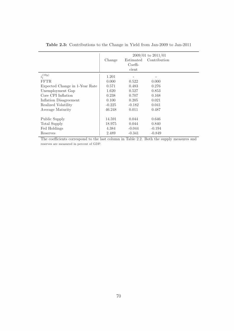
Table 2.3: Contributions to the Change in Yield from Jan-2009 to Jan-2011

2009/01 to 2011/01Change Estimated

Coeffi-cient

Contribution

i(10y)t 1.201 - -FFTR 0.000 0.522 0.000Expected Change in 1-Year Rate 0.571 0.483 0.276Unemployment Gap 1.620 0.527 0.853Core CPI Inflation 0.238 0.707 0.168Inflation Disagreement 0.100 0.205 0.021Realized Volatility -0.225 -0.182 0.041Average Maturity 46.248 0.011 0.487

Public Supply 14.591 0.044 0.646Total Supply 18.975 0.044 0.840Fed Holdings 4.384 -0.044 -0.194Reserves 2.489 -0.341 -0.849

The coefficients correspond to the last column in Table 2.2. Both the supply measures andreserves are measured in percent of GDP.

70

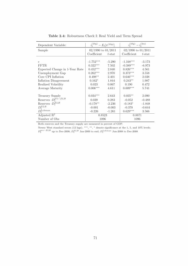
Table 2.4: Robustness Check I: Real Yield and Term Spread

Dependent Variable: i(10y)t − Et[π

(10y)] i(10y)t − i

(3m)t


c -1.752∗∗∗ -5.290 -1.348∗∗∗ -3.173FFTR 0.322∗∗∗ 7.502 -0.389∗∗∗ -6.973Expected Change in 1-Year Rate 0.452∗∗∗ 2.840 0.826∗∗∗ 4.561Unemployment Gap 0.262∗∗∗ 2.970 0.373∗∗∗ 3.558Core CPI Inflation 0.498∗∗ 2.401 0.646∗∗∗ 2.038Inflation Disagreement 0.162∗ 1.844 0.243∗∗ 1.987Realized Volatility 0.023 0.067 0.190 0.472Average Maturity 0.006∗∗∗ 4.611 0.009∗∗∗ 5.741

Treasury Supply 0.034∗∗∗ 2.643 0.035∗∗ 2.090

Reserves ·Dpre−ZLBt 0.039 0.283 -0.052 -0.488

Reserves ·DZLBt -0.178∗∗ -2.236 -0.183∗ -1.848

DZLBt -0.001 -0.003 -0.370 -0.644

DLehmant -0.226 -1.261 0.629∗∗∗ 3.566






71

Table 2.5: Robustness Check II: 5-Year Treasury Yield

Dependent Variable: i(5y)t i

(5y)t − Et[π

(5y)]


c -1.629∗∗∗ -3.219 -1.640∗∗∗ -4.590FFTR 0.616∗∗∗ 9.175 0.375∗∗∗ 8.133Expected Change in 1-Year Rate 0.059 0.229 0.026 0.141Unemployment Gap 0.483∗∗∗ 3.608 0.182∗ 1.426Core CPI Inflation 0.560∗ 1.782 0.331 0.515Inflation Disagreement 0.118 0.855 0.052 0.858Realized Volatility -0.521 -0.912 -0.322 -0.816Average Maturity 0.010∗∗∗ 4.934 0.005∗∗∗ 3.582

Treasury Supply 0.042∗ 1.958 0.034∗∗ 2.364

Reserves ·Dpre−ZLBt 0.093 0.530 0.080 0.658

Reserves ·DZLBt -0.453∗∗∗ -3.285 -0.313∗∗∗ -3.384

DZLBt 0.691 0.879 0.952∗ 1.791

DLehmant -0.535∗∗ -2.062 -0.443∗∗ -2.487






72

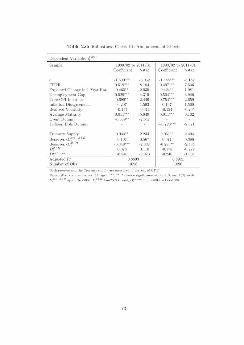
Table 2.6: Robustness Check III: Announcement Effects



c -1.500∗∗∗ -3.052 -1.588∗∗∗ -3.182FFTR 0.519∗∗∗ 8.184 0.497∗∗∗ 7.546Expected Change in 1-Year Rate 0.460∗∗ 2.035 0.424∗∗ 1.981Unemployment Gap 0.529∗∗∗ 4.315 0.504∗∗∗ 3.946Core CPI Inflation 0.699∗∗ 2.449 0.754∗∗∗ 2.659Inflation Disagreement 0.207 1.593 0.197 1.500Realized Volatility -0.157 -0.311 -0.134 -0.265Average Maturity 0.011∗∗∗ 5.849 0.011∗∗∗ 6.102Event Dummy -0.369∗∗ -2.547 - -Jackson Hole Dummy - - −0.728∗∗∗ -2.671

Treasury Supply 0.044∗∗ 2.234 0.051∗∗ 2.494

Reserves ·Dpre−ZLBt 0.107 0.567 0.071 0.386

Reserves ·DZLBt -0.348∗∗∗ -2.837 -0.285∗∗ -2.434

DZLBt 0.078 0.110 -0.178 -0.272

DLehmant -0.240 -0.973 -0.246 -1.003






73

C The Data

The analysis uses weekly data. Both the data on non-borrowed reserves and on the Fed’s

holdings of Treasury securities are available as end-of-Wednesday levels. We hence define

the beginning of a week as Thursday and the end as Wednesday. For the data available

on a daily basis, we compute one-week averages of the daily data on a weekly frequency.

Thus, given t− 1 corresponds to a Wednesday, then

it =1

5

4∑s=0

it+s for {it, it+5, . . .} (2.2)

The data available only at a lower frequency are linearly interpolated, matching the

monthly observation with the last week’s observation of the month. Accordingly, Fig-

ures 2.3 to 2.5 depict the final data entering the regressions.

The 5-year and 10-year Treasury bond yields are from Datastream. Real 5-year and 10-

year yields are constructed using the Fisher equation and data on inflation expectations

at the two horizons from the Federal Reserve Bank of Cleveland.12

The Federal Funds target rate (FFTR) is retrieved from the FRED (DFEDTAR). It

starts in 1982, but is discontinued after 2008. We therefore link it with recent data from

Bloomberg.

Core CPI inflation is retrieved from the BIS. The unemployment gap is measured as the

difference between the monthly unemployment rate retrieved from Datastream and the

Congressional Budget Office’s estimate of the NAIRU.13 As in Gagnon et al. (2010), long-

run inflation disagreement is measured as the interquartile range of 5- to 10-year ahead

inflation expectations, as reported by the Michigan Survey of Consumers.14 The six-month

12The Cleveland Fed’s data on inflation expectations can be downloaded from http://www.clevelandfed.

org/research/data/inflation_expectations/index.cfm.

13The CBO’s estimate of the NAIRU can be downloaded from http://www.cbo.gov/doc.cfm?index=

12039.

14This data can be downloaded from http://www.sca.isr.umich.edu/main.php.

74

realized daily volatility is computed using a rolling 24-week window of the 10-year Treasury

yield.

Gagnon et al. (2010) use the Eurodollar slope as a proxy for interest rate expectations.

They use the difference between the implied rates on Eurodollar futures contracts settling

approximately two-years and one-year ahead. We approximate the 2-year-ahead Eurodollar

rate by the implied 1-year forward rate from 2-year and 3-year Treasuries. Similarly, we

approximate the 1-year-ahead Eurodollar rate by the implied 1-year forward rate from

1-year and 2-year Treasury yields. The expectations hypothesis defines the 2-year and the

3-year Treasury yields as follows.

1 + i(2y)t =

(1 + i

(1y)t

)(1 + Eti

(1y)t+1

)(2.3)

1 + i(3y)t =

(1 + i

(2y)t

)(1 + Eti

(1y)t+2

)(2.4)

The expected 1-year rate one year and two years ahead are thus

Eti(1y)t+1 =

1 + i(2y)t

1 + i(1y)t

− 1, and (2.5)

Eti(1y)t+2 =

1 + i(3y)t

1 + i(2y)t

− 1. (2.6)

To get the expected change of the 1-year rate one year ahead, we use the difference between

the two, i.e. Eti(1y)t+2 − Eti

(1y)t+1 .

For the Treasury supply, we use the data provided by Hamilton and Wu (2010b)15 as well

as data directly retrieved from the SOMA.16 Hamilton and Wu provide data on total Trea-

sury supply and on Treasury supply to the public, calculated as total supply minus Fed

holdings. The periodicity of their data is monthly. Since the SOMA provides weekly data

as of Wednesdays, we compute the public supply ourselves. Unfortunately, the data from

15Hamilton and Wu (2010b) provide their data on the Treasury supply from http://econ.ucsd.edu/

~jingwu/zlb_data.html.

16The data on the Factors Affecting Reserve Balances (H.4.1) is published by the Board of Gover-nors of the Federal Reserve System and can be downloaded from http://www.federalreserve.gov/

datadownload/Choose.aspx?rel=H41, Table 2.

75

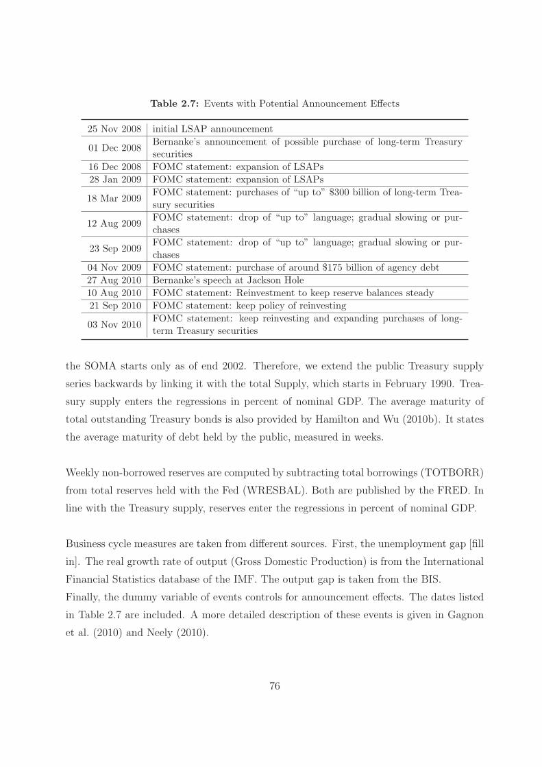
Table 2.7: Events with Potential Announcement Effects

25 Nov 2008 initial LSAP announcement

01 Dec 2008Bernanke’s announcement of possible purchase of long-term Treasurysecurities

16 Dec 2008 FOMC statement: expansion of LSAPs

28 Jan 2009 FOMC statement: expansion of LSAPs

18 Mar 2009FOMC statement: purchases of “up to” $300 billion of long-term Trea-sury securities

12 Aug 2009FOMC statement: drop of “up to” language; gradual slowing or pur-chases

23 Sep 2009FOMC statement: drop of “up to” language; gradual slowing or pur-chases

04 Nov 2009 FOMC statement: purchase of around $175 billion of agency debt

27 Aug 2010 Bernanke’s speech at Jackson Hole

10 Aug 2010 FOMC statement: Reinvestment to keep reserve balances steady

21 Sep 2010 FOMC statement: keep policy of reinvesting

03 Nov 2010FOMC statement: keep reinvesting and expanding purchases of long-term Treasury securities

the SOMA starts only as of end 2002. Therefore, we extend the public Treasury supply

series backwards by linking it with the total Supply, which starts in February 1990. Trea-

sury supply enters the regressions in percent of nominal GDP. The average maturity of

total outstanding Treasury bonds is also provided by Hamilton and Wu (2010b). It states

the average maturity of debt held by the public, measured in weeks.

Weekly non-borrowed reserves are computed by subtracting total borrowings (TOTBORR)

from total reserves held with the Fed (WRESBAL). Both are published by the FRED. In

line with the Treasury supply, reserves enter the regressions in percent of nominal GDP.

Business cycle measures are taken from different sources. First, the unemployment gap [fill

in]. The real growth rate of output (Gross Domestic Production) is from the International

Financial Statistics database of the IMF. The output gap is taken from the BIS.

Finally, the dummy variable of events controls for announcement effects. The dates listed

in Table 2.7 are included. A more detailed description of these events is given in Gagnon

et al. (2010) and Neely (2010).

76

Chapter 3

Central Bank Reserves and the Yield

Curve at the ZLB

Abstract

With short-term interest rates bounded at zero, monetary policy has aimed at affecting the

yield curve at the longer end during the recent years. As the recent literature has shown, the

quantitative easing programs conducted by the Federal Reserve have significantly lowered

long-term yields. This paper adds central bank reserves as a fourth factor to an affine

term structure model to estimate the effect of quantitative easing on the yield curve. The

cumulative effect on 10-year Treasury securities during the zero lower bound period is

estimated to amount to 85 basis points. Of the total effect, one quarter is shown to be

due to the liquidity effect and three quarters to the supply effect. To disentangle the two

effects, the estimates for the US are compared to estimates for Swiss data because the

Swiss national bank did not engage in any government bond purchases.

77

1 Introduction

Central banks around the globe have been flooding financial markets with liquidity since

the breakdown of interbank markets in response to the collapse of Lehman Brothers in the

fall of 2008. In its initial phase of unconventional monetary policy, also referred to as QE1,

the US Federal Reserve performed large scale asset purchases (LSAP) consisting mainly

of mortgage-backed securities. The Federal Reserve then gradually extended liquidity by

outright purchases of Treasury securities. When the Treasury purchase program known

as QE2 came to an end in mid 2011, non-borrowed reserves (NBR) held at the Federal

Reserve exceeded USD 1.6 Trillion.

Aside from signalling effects about future policy, the literature has focussed mainly on

portfolio balance effects of outright Treasury securities’ purchases of the Federal Reserve1,

in particular the so-called supply effect and spill over effects from outright purchases of

similar assets such as mortgage backed securities and agency debt2. Krogstrup et al. (2012)

have shown that, in addition to the supply effect, there is also a liquidity effect of quan-

titative easing (QE) that has affected long-term Treasury bonds. While the supply effect

depends on the composition of the central bank’s balance sheet, it is an expansion of the

balance sheet that triggers the liquidity effect.

This study proceeds in two steps: it first estimates the total effect of QE on term premia in

an Affine Term Structure Model (ATSM) framework; in a second step it attempts to disen-

tangle the supply from the liquidity effect. Our estimates show that QE has significantly

lowered the term premium of Treasury yields. Estimates of the cumulative effect of QE

on 10-year Treasury yields during the zero lower bound (ZLB) amounts to 85 basis points.

This result is in line with the recent literature. Estimates of Swiss data suggest 10-year

yields decreased 34 basis points in response to the expansion in liquidity. Because the Swiss

National Bank (SNB) has not engaged in government bond purchases during the ZLB, the

Swiss estimates can be fully ascribed to the liquidity effect. In the US, approximately 21

1See e.g. Gagnon et al. (2011), Hamilton and Wu (2010b), Krishnamurthy and Vissing-Jorgensen (2011)

2See e.g. D’Amico and King (2010)

78

basis points can be attributed to the liquidity effect and 64 basis points to the supply effect.

QE may affect either the expectations’ part of interest rates or the term premium. While

signalling effects change expectations about future policy, the supply and the liquidity ef-

fect operate on the term premium. Term structure models are suitable to isolate the term

premium. The three latent factors are typically shown to account for changes in expected

future interest rates and thus capture any signalling effects and announcement effects that

affect expectations about the future policy rate. Christensen and Rudebusch (2012) isolate

the term premium in an affine term structure model and find that in US data, most of the

effect of QE on yields was transmitted through policy expectations rather than the term

premium. Hence, they find that the portfolio balance effect - or the supply effect - of QE

on yields was much smaller than the signalling effect in the US. Information theory would

suggest that the supply effect materializes immediately after announcements of the asset

purchases. Therefore, many papers3 apply event studies to estimate the effects. Instead,

we add a fourth factor to the term structure model, a measure for liquidity, to explain

changes in the term premium. The main analysis is computed for US data, divided into

two subsamples: a pre-crisis sample that should account for “normal” times and a ZLB

sample. To better separate the supply effect from the liquidity effect, we additionally run

the analysis for Swiss data as a counterfactual case. The injected liquidity by the SNB

was entirely driven by foreign exchange purchases rather than government bonds. Hence,

a supply effect can be excluded.

The rest of the paper is organized as follows. Section 2 lays out the different effects of

quantitative easing on yields. Section 3 illustrates the US and Swiss data sets. Section 4

introduces the term-structure model used and Section 5 provides the details on the model

estimation. Finally, Section 6 presents the results and Section 7 concludes.

3See for example Gagnon et al. (2010) and Bauer and Rudebusch (2011).

79

2 The Different Effects of QE on Interest Rates

The recent literature has focused on two effects of the Federal Reserves’ asset purchases.

Fist, measures undertaken by the monetary authority are typically thought to have a

signaling effect about future monetary policy. For example, Christensen and Rudebusch

(2012) find that most of the declines in US interest rates can be attributed to lower policy

expectations. Second, the purchase of long-term assets changes the maturity structure of

the assets available to the public which might trigger a portfolio balance effect. Accord-

ingly, Gagnon et al. (2011) attribute most of the effect of the LSAP on long-term yields to

this portfolio balance effect, the so-called supply effect. Krogstrup et al. (2012) suggest a

third mechanism at work: a liquidity effect on longer-term yields. Conversely to the first

two effects, the liquidity effect hinges on the expansion rather than the composition of a

central banks’ balance sheet. By augmenting its balance sheet, the central bank creates

additional funding and provides it to the economy, so there is more funding available to

finance an unchanged amount of debt. Krogstrup et al. (2012) argue that some of the

additional credit might have found its way into Treasury bonds and thereby brought down

long-term yields.

The signalling effect can be clearly distinguished from the other two as it affects the expec-

tations’ part of yields rather than the term premium. It is not straightforward, however,

to disentangle the liquidity effect from the supply effect. With an outright purchase of a

Treasury bond, the Federal Reserve temporarily raises demand and therefore the price of

that bond. Since the bond is drawn from the market, the supply of that bond decreases.

Given unchanged market demand for this specific bond, the price increases and the yield

decreases permanently. This effect is referred to as the supply effect in the literature.4

The supply effect boils down to a portfolio balance effect that arises if there is some kind

of “preferred-habitat” behavior of investors, e.g. if investors have a preference for the spe-

cific maturity of the asset purchased by the central bank. Some research suggests that

this portfolio balance effect might even be at work across different asset classes. D’Amico

and King (2010), for example, suggest that the purchases of mortgage backed securities

4See e.g. Hamilton and Wu (2010a), Vayanos and Vila (2009), Greenwood and Vayanos (2010), Neely(2010), Kuttner (2006), D’Amico and King (2010) for recent research on the supply effect.

80

conducted by the Fed significantly affected long-term Treasury yields. In addition to the

supply effect, the price change will spread to close-by maturities due to arbitrage. That

said, an outright purchase of an asset conducted by the central bank raises the amount of

credit in the form of reserves available in the aggregate. Assuming an unchanged amount

of government debt, i.e. Treasury bonds, prices of these bonds will, all else equal, increase

as there is more money to buy the same amount of assets. This is what Krogstrup et al.

(2012) refer to as the liquidity effect.5 The liquidity effect in the sense of Friedman (1968)

refers to a fall in short-term nominal interest rates after an exogenous persistent increase

in narrow measures of the money supply.6 When the policy rate hits the zero lower bound

(ZLB), the liquidity effect on the short-term yields is arguably absent, as the short-term

Treasury bills and money become equivalents. However, as the banks that sell assets to

the central bank hold more money after the transaction, they might seek a positive return

further out the yield curve.

The supply and the liquidity effect are difficult to distinguish empirically. The expansion of

the Federal Reserve’s balance sheet was largely due to the purchase of US Treasury bonds.

Thus, the change in the supply of bonds, measured as the quantity of these bonds held by

the Federal Reserve, is correlated with the amount of liquidity, measured as the deposits

banks hold at the Federal Reserve. We address this difficulty by comparing estimates from

US data with those from Swiss data. In the case of Switzerland, the supply effect cannot

have been at play as the SNB increased liquidity through purchases of foreign exchange

rather than government bonds.

5The amount of money relative to the volume of assets increases, ceteris paribus, against the entire spec-trum of assets. So the same price effect might be observed for other assets, too. The effect on Treasurybonds might be particularly large because these assets are very safe and liquid. Krishnamurthy andVissing-Jorgensen (2011) argue that these characteristics make government bonds constitute a close sub-stitute for money.

6See e.g.Thornton (2008b).

81

3 Data

The following section briefly describes and illustrates both the US and the Swiss data sets

used and explains how we conduct our analysis in two subsamples, one corresponding to

“normal times” and another to the ZLB period.

3 .1 US Data

The analysis is conducted on a weekly basis, so the data is converted into the same fre-

quency. The sample spans from June 2005 to October 2011. Because NBR data are

published on Wednesdays, all data are snapshots as of that day. Interest-rate data used

stem from off-the-run US Treasury Bills and Bonds. In particular, we use 3-month and 6-

month secondary market T-bills rates7 and 1-year to 10-year off-the-run constant maturity

yields from Gurkaynak et al. (2007)8. All the yields are continuously compounded, whereas

quarterly and semi-annual compounding is assumed for the 3-month and the 6-month rate,

respectively.9

In the literature, different measures of money have been used to analyze the liquidity effect.

As concluded by Pagan and Robertson (1995), models defining money as narrow measures

are more successful in giving evidence for a liquidity effect than those using broader mea-

sures of money. This is due to the fact that shocks to broader monetary aggregates are

largely due to shocks in money demand rather than to shocks in money supply.10 Hence,

the expansion in liquidity conducted by the Federal Reserve is measured by the amount

of reserves banks hold with the Federal Reserve. Total reserves are often found not to

correlate with interest rates because the part of reserves which is borrowed is driven by the

bank’s demand for reserves. This makes borrowed reserves endogenous, as the demand for

7Obtained from the Federal Reserve Economic Data base (FRED), under DTB3 and DTB6. The two arenot constant-maturity yields which is acceptable due to their short maturity.

8The data can be downloaded from http://www.federalreserve.gov/econresdata/researchdata.htm.We use off-the-run treasuries to avoid the treatment of “repo-specialness” implicit in the on-the-runTreasury securities, see Duffie (1996) and Jordan and Jordan (1997).

9See Hull (2008).

10See e.g. Bernanke and Blinder (1992), Sims (1992), or Christiano and Eichenbaum (1995).

82

liquidity responds to monetary policy changes.11 We therefore use NBR, i.e. total reserves

minus borrowed reserves,12 as the measure of liquidity.

The main hypothesis of the paper is that liquidity effects are present at the longer end

of the yield curve only when interest rates are close to the ZLB. Therefore, the analysis

is carried out in two subsamples. The first can be characterized as “normal times” with

interest rates far away from the ZLB. It is defined as starting with the first week of June

2005 until the end of July 2007.13 The second subsample corresponds to the ZLB period.

It starts with the second week of December 2008, when the Federal funds rate reached the

ZLB, and runs through October 2011, the end of the sample (see Figure 3.1).

Figure 3.1 depicts the data. The NBR fluctuated around the level of 10 billion USD in the

first subsample shown in the upper panel. NBR amounted to roughly 540 billion USD at

the time the Federal funds rate reached the ZLB in late 2008. Then, during the ZLB period

shown in the lower panel, NBR continued to grow to reach 1,560 billion USD by October

2011. In the first and the second subsample, the standard deviation of NBR equals 2.9

and 318.5 billion USD, respectively. In order to make the estimation results from the two

periods comparable, the NBR factor is normalized so that it exhibits a standard deviation

of one within each subsample.

3 .2 Swiss Data

The data used in the analysis are the 3-month and the 6-month CHF Libor rates and 1-

year to 10-year constant-maturity zero-coupon yields on Swiss Confederation Bonds. The

data on giro account balances (i.e. sight deposits) of both domestic and foreign banks at

the SNB is used to measure liquidity. The SNB publishes this data on a weekly basis, so

11See e.g. Carpenter and Demiralp (2008).

12Borrowed reserves are equal to the sum of credit extended through the Federal Reserve’s regular discountwindow programs and credit extended through certain Federal Reserve liquidity facilities. The totalreserves (WRESBAL) and the total borrowings (TOTBORR) are also available from the FRED.

13We could have used a longer sample for the non-ZLB period. Trying different sample lengths andstart/end points does not change the non-ZLB results.

83

the analysis can also be conducted at the weekly frequency. In line with the US case, we

choose the two subsamples so that one corresponds to “normal times” and the second to

the ZLB period. The former subsample starts in the first week of January 2006 and ends

on 12 September 2008.14 The second subsample starts with the second week of December

2008, when the SNB decreased its targeted level for the 3-month Libor from 1% to 0.5%,

and ends on 7 October 2011.

3 .3 Simple Data Inspection

Figure 3.1 presents US data and Figure 3.2 Swiss data, where the upper panels show the

earlier subsample and the lower panels depict the ZLB period. It is very difficult to see any

comovement between interest rates and NBR in both samples in either data set. To get

a first idea on such a comovement, Table 3.1 depicts correlations between different yields

and NBR. The numbers are reported for both the US and Switzerland. In the upper panel,

the correlation refers to levels, whereas the lower panel computes the correlations in first

differences. The simple correlations draw a mixed picture.

Macroeconomic theory holds that, in normal times, the liquidity effect dominates at the

short end of the yield curve, while at the longer end the Fisher effect is thought to obscure

the liquidity effect. Hence, we would expect the correlation between NBR and short-term

yields to be negative, while the correlation with long-term yields would turn positive with

rising inflation expectations. As Table 3.1 shows in the first row, the data does provide

evidence for the liquidity effect as correlations are negative in the US data. The negative

correlation weakens with maturity, however, suggesting that the dominance of the Fisher

effect increases as we move out on the yield curve. The Swiss data provides the exact

opposite picture; there is no evidence for a liquidity effect, and the Fisher effect seems

to decrease with maturity. Correlations decrease considerably during the ZLB period for

both countries. In US data the negative correlation is largest around the 1-year maturity

while the Swiss data suggests longer maturities to be affected the most.

14The exact choice of the “normal times” subsample does not affect the results. Preliminary analysis ofseveral different non-ZLB subsamples showed no liquidity effect irrespective of the exact period.

84

4 The Model

This section defines the term structure model we use to estimate the liquidity effect. We

start from the general asset pricing equation, define the pricing kernel and specify a Gaus-

sian diffusion process of the underlying state factors. Then, we specify the one-period

interest rate and formulate the bond prices across the maturity spectrum.

4 .1 General Setting and State Dynamics

The general asset pricing equation15 under the physical probability measure P reads

Pn,t = Et [Mt+1Pn−1,t+1|It] , (3.1)

where Pn,t is the price of an n-period to maturity zero-coupon bond at time t, Mt+1 denotes

the stochastic discount factor, and It represents the agents’ current information set. In

a risk-neutral world, where investors request no risk compensation, the price of the bond

Pn,t equals

Pn,t = EQt [exp(−y1,t)Pn−1,t+1|It] , (3.2)

where Q is the risk-neutral probability measure and y1,t is the short-term interest rate. The

no-arbitrage argument assures that the two prices in (3.1) and (3.2) are equal. There exists

an equivalent martingale measure Q according to which (3.2) holds16 with the stochastic

discount factor taking the form

exp(−y1,t) = Et [Mt+1|It]= exp(−y1,t)Et [(dQ/dP)t+1|It] .

15See Campbell et al. (1997).

16See Harrison and Kreps (1979).

85

dQ/dP is the Radon-Nykodim derivative17 which follows a log-normal process, so it reads

(dQ/dP)t+1 = exp

(−1

2(λt)

′λt − (λt)′εt+1

). (3.3)

λt is the market price of risk associated with the sources of uncertainty εt.18 Following

Duffee (2002), the market price of risk is an “essentially affine” function of the state

variables Xt, so it can be written as

λt = λ0 + λ1Xt. (3.4)

Equations (3.3) to (3.4) jointly define the pricing kernel of the model, where the essentially

affine market price of risk constitutes the first fundamental building block of the Gaussian

term structure model.

Another fundamental building block of the Gaussian term structure model is the multi-

variate state variable Xt. It follows a discrete version of the constant volatility Ornstein-

Uhlenbeck process.19 Under the physical probability measure P, the process is

Xt+1 = (I −Ψ)μ+ΨXt + Σεt+1. (3.5)

The first term on the right-hand side of equation (3.5) is a vector of the factors’ means. Ψ

is the VAR matrix and Σ is the covariance matrix that normalizes the residuals εt which

are assumed to be standard normal i.i.d. shocks.

4 .2 Short Rate and Bond Prices

Following Duffie and Kan (1996), the one-period interest rate

y1,t = A1 +B1Xt

is an affine function of risk factors Xt, where the coefficient A1 corresponds to the average

17See Dai et al. (2007).

18See Ang and Bekaert (2002) and Ang and Piazzesi (2003).

19See Phillips (1972).

86

one-period rate in the sample and B1 is a vector of loadings of the risk factors on y1,t. The

risk factors are

Xt =

⎡⎢⎢⎢⎢⎢⎣

l1,t

l2,t

l3,t

Rt

⎤⎥⎥⎥⎥⎥⎦ (3.6)

The first three factors lit, i = 1, 2, 3 denote the latent factors backed out from yields, Rt

denotes central bank reserves. As commonly in the term structure literature, these factors

can be interpreted as a level, a slope, and a curvature factor.20 In order to estimate the

liquidity effect on the longer end of the yield curve, this paper adds central bank reserves

as a fourth factor to Xt.21 As it can be noticed, the model assumes no ZLB for the short

rate. Yet, as shown in the results section, the model fits the data reasonably well and thus

can be considered as a good approximation.

Assuming joint log-normality of bond prices and the pricing kernel in equation (3.1), the

n-periods to maturity nominal bond price is an affine function of the state variables22 and

thus takes the form

pn,t = −An − BnXt (3.7)

with

An = An−1 +Bn−1 ((I −Ψ)μ− Σλ0) +1

2Bn−1ΣΣ

′B′n−1 + A1

Bn = Bn−1 (Ψ− Σλ1) + B1.

(3.8)

20See Section 5 for more details on “backing out” of the yield-only factors.

21Ang and Piazzesi (2003), for instance, are among many studies that use macro-economic variables asexplicit factors.

22See for example Cochrane and Piazzesi (2009).

87

5 Estimation

This section derives the likelihood function used to construct the joint posterior of param-

eters and data. In addition, the model is estimated with a simple version of the Bayesian

Markov-Chain Monte-Carlo (MCMC) method and this section provides the general idea,

rationale and the description of the algorithm.

5 .1 Likelihood Function

Following Chen and Scott (1993), the 6-month, the 5-year and the 10-year yields are set

to be observable, while the rest is measured with an error. Let yo,t be a vector of observed

yields that are perfectly priced by the model. Then, equation (3.7) can be written as

[yo,t

Rt

]=

[Ao

01×1

]+

[Bo 03×1

01×3 1

][Xo,t

Rt

],

where Ao is a 3× 1 vector and Bo a 3× 3 matrix of factor loadings. Xo,t contains the three

latent factors obtained by inverting the above equation as:

[Xo,t

Rt

]=

[Bo 03×1

01×3 1

]−1 ([yo,t

Rt

]−

[Ao

01×1

])

The first part of the likelihood function refers to the evolution of the state variables Xt as

given in equation (3.5). The assumption that εt is multivariate-Gaussian implies that the

conditional probability density function of Xt is

f (Xt | yo,t−1, Rt−1) =exp

(−12ε′t (Σ

′Σ)−1 εt)

√(2π)T | Σ′Σ | . (3.9)

Let the yu,t be a vector of remaining N − 3 yields priced by the model with an error:

yu,t = Au +BuXt + ξt.

The second part of the likelihood function refers to the pricing errors ξt. They are assumed

to be distributed as i.i.d. N (0, ω2I), with the identical ω2 and zero correlations across

yields. I is a unity matrix. The conditional density of yu,t is thus given by

88

f (yu,t | Xt) =exp

(−1

2ξ′t((ω2I)

′ω2I

)−1ξt

)√

(2π)T∣∣(ω2I)′ ω2I

∣∣ . (3.10)

The log-likelihood function is just the sum of logarithms of the “time-series part” in equa-

tion (3.9) and the “cross-sectional part” in equation (3.10) and thus takes the form

lnL(·) = log(f (Xt | yo,t−1, Reservest−1)) + log(f (yu,t | Xt)). (3.11)

5 .2 Econometric Identification

Solid identification of parameters is an essential part of dynamic term structure model esti-

mation. The proposed identification scheme follows Dai and Singleton (2000) and Hamilton

and Wu (2010a).

To begin with, the upper-left block of the VAR matrix Ψ, i.e. the matrix driving the

dynamics of the yields-only factors in Xo,t, is set to be a power law structure,23 with zero

non-diagonal elements and the following power relation on the diagonal:

ψzz = ψ11αz−1.

ψ11 is the largest eigenvalue of Ψ. The AR coefficient of the first latent factor α serves as a

scaling parameter controlling the distance between the eigenvalues, and z = 2, ...Z, where

Z is the number of latent factors. Preliminary estimation showed that the ψ11 parameter

is near one. In line with the near co-integration assumption from previous studies,24 we

simply set ψ11 to 1,25 and estimate ψzz, where z = {2, 3}, together with the AR(1) coeffi-

cient of the reserves dynamics. The off-diagonal elements of the Ψ are set to zero, as well

as the μ vector and the off-diagonal elements of matrix Σ in the transition equation (3.5).

We impose the usual boundary condition A0 = B0 = 0 on the parameters of the pricing

23See also Calvet et al. (2010) and Bauer and de los Rios (2011).

24See for instance Giese (2008) and Jardet et al. (2011).

25As in Diebold and Li (2006), Soderlind (2010) and Bauer (2011).

89

equation given in (3.7). A1 is normalized to average the one-period interest rate in the

sample26 while B1 is normalized to [1 1 1 bReserves]′ .27

Finally, the market price of risk dynamics is restricted to

λst =

⎡⎢⎢⎢⎢⎢⎣

λ0,1

λ0,2

0

0

⎤⎥⎥⎥⎥⎥⎦+

⎡⎢⎢⎢⎢⎢⎣

0 0 0 λ1,14

0 0 0 λ1,24

0 0 0 0

0 0 0 0

⎤⎥⎥⎥⎥⎥⎦Xt, (3.12)

so that both “level” and “slope” risks are priced in yields.28 This is the main market

price of risk specification of the study. The results are also reported for the risk-neutral

Q measure, where λ0 = λ1 = 0 and for the case where only the “level” shock is being a

compensated risk, i.e. where λ0,2 and λ1,24 are set to 0.29

5 .3 Bayesian Inference

The yield curve implied by the model is a complicated non-linear function of the underlying

parameters. As such non-linearity tends to produce a multi-modal likelihood function,30

it is a daunting task to fit a yield curve model with a standard maximum likelihood

estimation. The Bayesian Markov Chain Monte Carlo (MCMC) method is a powerful

alternative that provides both efficiency and tractability.

Setting

Let Θ be a vector of length K that collects all the parameters of the model to be estimated:

Θ = {α, ψR,Σ, λ0, λ1, ω, bR} .26Following Favero et al. (2007).

27As in Ang et al. (2008). Alternatively, one could set the covariance matrix of the transition equation(3.5) to a unity matrix and estimate all the elements of B1 as for instance in Ang and Piazzesi (2003).

28As in Duffee (2010) and Joslin et al. (2010).

29We follow the specification in Cochrane and Piazzesi (2009) and add the slope factor. It is indeed arestricted set of models, yet previous studies show that many restrictions on the market price of risk aresupported by the data, see Joslin et al. (2010) and Bauer (2011).

30See Chib and Ergashev (2009).

90

The key idea behind Bayesian estimation is to consider the vector as a multivariate random

variable and to use the Bayes’ rule to “learn” about the variable given the data observed.

The posterior density of Θ

p (Θ | data) = p (data | Θ) p (Θ)

p (data), (3.13)

where p (data | Θ) is the likelihood function and p (Θ) denotes the prior density of the

parameters. The term p (data) is known as ”normalizing constant” and is independent of

Θ.31 Consequently, the rule in (3.13) can be re-written as

lnp (Θ | data) ∝ lnL+ lnp (Θ) ,

where

lnL =T−1∑t=0

lnpdf (Xt | yo,t−1, rt−1)

+T−1∑t=0

lnpdf (yu,t|Xt, yo,t−1, rt−1)

(3.14)

is the logarithm of the likelihood function defined in (3.9) and (3.10).

Priors

In the estimation, the priors p (Θ) are set to be non-informative or ”flat”, so that the pos-

terior density of the model parameters is drawn with equal probability from the pre-defined

support interval. Alternatively, we could derive the prior distributions for parameters Ψ

and Σ, given the normality assumption of the state VAR process,32 and for ω given the

assumption of the Gaussian measurement error.33 Chib (2001) proposes a scaled beta

distribution as an alternative to the uniform distribution. Nevertheless, we choose not to

31In particular, p (data) =∫p(data | Θ)p(Θ)dΘ. See Koop (2003).

32For instance, see Ang et al. (2007).

33See for example Mikkelsen (2001).

91

impose lower (or higher) probability areas from which the candidate values of parameters

are drawn. This way, the estimation is almost completely data-driven and proves to be

computationally efficient.

The parameters’ support intervals are specified by following the no-arbitrage condition and

previous studies. In particular, the eigenvalues of the VAR matrix are set to be positive

and less than one and the volatility parameters on the diagonal of Σ are set to be non-

negative. The parameter bNBR is constrained to lie inside the unit-circle. The lower bound

of the parameters in vector λ0 and matrix λ1 are set as in Chib and Ergashev (2009).

Markov Chain Monte Carlo

We use a simple version of the “Metropolis within Gibbs” algorithm34 to draw the param-

eters from their posterior densities. The parameter candidates are drawn from continuous

uniform distributions U(Θ,Θ

)where the lower and the upper boundaries Θ and Θ for

each parameter in Θ are specified in Table 3.2. The algorithm can be described in five

steps.

Step 1: Set the initial values for the parameters Θ0. Set up two Markov chains with dif-

ferent starting values. The initial values for the VAR parameters in the first chain are

obtained from OLS and the data descriptive statistics. The starting values of the market

price of risk parameters and of the second chain are chosen arbitrarily.35

Step 2: Draw a candidate log-posterior density lnp (Θ∗ | Θmc−1, data) conditional on pre-

viously drawn parameter values Θmc−1. The number mc denotes current iteration. The

34The “Metropolis within Gibbs” algorithm is a simple method and therefore often used in the literature,as for example in Gilks (1996), Koop (2003) and Lynch (2007). In particular, this algorithm featurestwo favorable characteristics. First, in standard Metropolis new proposals for the parameter values aredrawn all at once whereas the Gibbs sampler draws only one proposal for only one parameter value ata time. Therefore, the Gibbs sampler results much more efficient, i.e. the estimator converges quicker.Second, the tuning of the estimator is simpler, where tuning refers to setting the scale factor in step 2to different values. In standard Metropolis, one scale factor must “fit all”. The Gibbs sampler is moreflexible as it allows for a separate set of values for each parameter.

35For example, the volatility parameters’ starting values are set to be 3 times larger in the second chain,the Ψ matrix parameters are set to 0.8 and the B1 parameter is set to 0.5 and -0.5 in the first and thesecond Markov chain, respectively.

92

draws are performed separately for every parameter in Θ. For instance, a proposal for the

first element in the vector Θ is generated by the Markov chain

θ∗1 = θmc−11 + ν1U1,

where νk is a scaling factor and Uk is an uniformly distributed random number from the

interval [-1,1]. We initialize νk for parameters α and ψNBR to 0.01, for the diagonal ele-

ments of matrix Σ and the market price of risk parameters to 0.1, and for the ω parameter

to 0.00001.36 The scaling factor is then automatically updated after every 5,000 sweeps to

obtain an acceptance ratio in step 4 of approximately 0.5.

Step 3: For every parameter in Θ∗, calculate the difference between the posterior density

of the candidate value and the posterior density of the previously drawn parameter value,

keeping the other parameter values unchanged. Using again the first element in Θ as an

example, the difference reads:

δ = lnp({θ∗1, θmc−1

2 , ..., θmc−1K } | Θmc−1, data

)− lnp

({θmc−11 , θmc−1

2 , ..., θmc−1K } | Θmc−1, data

)(3.15)

Step 4: Draw a random number u ∼ U(0, 1) and accept the single parameter candidate

from Step 2 whenever

min(0, δ) > log(u)

holds for the difference in Step 3.

Step 5: Repeat steps 2 to 5 until the joint posterior density of parameters converges in

distribution.

36Proposed in Ang et al. (2007) so that it roughly corresponds to a 30 basis points bid-ask spread onTreasuries. An average spread on the OTC plain vanilla swap market might be similar. See also Skarr(2010).

93

The algorithm is run 100,000 times and the first 40,000 are discarded as the burn-in period.

The two Markov chains with different starting values for both joint posterior and the

single parameters’ posteriors converge to literally the same posterior distributions. Before

estimating the entire model, the proposed parametrization is used to estimate the risk

neutral specification. The model under Q converges even quicker37 and thus the algorithm

is run for 50,000 times and the first 20,000 are discarded as burn-in.38

6 Results

QE may affect either the expectations’ part of interest rates or the term premium - or both.

Term structure models as applied in this paper are suitable to isolate the term premium.

Therefore, the three latent factors should account for changes in expected future interest

rates. Central bank reserves as a fourth factor are added to explain changes in the term

premium. Our model performs well in that most of the variation in yields is explained by

three latent factors. The fourth factor contributes only marginally and it is only slightly

correlated with the latent factors. Our estimates show that QE has significantly lowered

the term premium of long-term Treasury yields. Estimates of the cumulative effect of QE

on 10-year Treasury yields during the ZLB amounts to 85 basis points. This result is in

line with the recent literature. Estimates of Swiss data suggest 10-year yields decreased

34 basis points which can be fully ascribed to the liquidity effect because the SNB did

not purchase government bonds to expand liquidity. In the following, this section lays

out the model performance and then presents the estimation results and the economic

interpretation. Finally, the supply and the liquidity effect are disentangled. As described

above, the model is estimated under three different settings concerning the price of risk.

Accordingly, the results are reported for the three different models.

6 .1 Model Performance

Table 3.2 and ?? report the parameter estimates for the two subsamples for US and Swiss

data, respectively. The tables report the estimated posterior modes of the parameters

37On average after 7,000 sweeps, between the non-ZLB sample and the ZLB sample.

38The scaling factor is also automatically adapted until the 20,000th iteration.

94

together with numerical standard errors (in brackets) for the subsample away from the

ZLB (ΘnonZLB) and the subsample at the ZLB (ΘZLB). The first two columns provide the

support intervals, and the last two the average acceptance ratios and inefficiency factors

(IF) for the two subsamples.39

Table 3.4 reports the cross-sectional fit for both countries and the two subsamples. By

construction, the 3-month, the 5-year and the 10-year yields are explained perfectly by the

model. The results are therefore not reported for these maturities. During the ZLB pe-

riod, the shorter end of the yield curve approached zero. This lower bound brought down

interest rate volatility at shorter maturities. Therefore, the pricing performance during

the ZLB period clearly outperforms the pre-ZLB pricing performance at the shorter end

of the yield curve. Comparing the different market price of risk settings, the time-varying

level and slope risks clearly improve the fit above the Q model. This is true especially in

the second subsample at mid to long maturities. Letting NBR affect the market price of

risk considerably improves the fit only in the ZLB-subsample. Thus, the choice of market

price of risk specification turns out to be relatively more important in the ZLB period

than in the pre-crisis sample. The fit also improves in the earlier subsample, but the gain

is relatively smaller. Allowing NBR to additionally affect the slope risk improves the fit

further at longer maturities only during the ZLB period. During normal times, as in the

earlier subsample, the addition of the time-varying slope risk lowers the fit.

A broad consensus in the term structure models literature is that the first three yields-only

factors account for most of the movements in the cross-section of yields.40 Figure 3.4 shows

the estimated latent factors in the two subsamples. Comparing the evolution of the latent

factors with the yield curve depicted in Figure 3.1 shows that the first latent factor seems

to drive the level movements of the yield curve in both periods, being relatively stable in

the first period and substantially increasing in volatility in the second. The second latent

factor l2 seems to move the slope of the yield curve, but this is only clear in the non-ZLB

period. The third latent factor l3 co-moves to a great extent with the second factor l2.

39The two indicators are explained in the tables’ headings.

40One of the key contributions in this field is Litterman and Scheinkman (1991).

95

The correlation in levels between the two factors amounts to -0.75 and -0.94 in the first

and the second subsample, respectively. Ang and Piazzesi (2003) and Joslin et al. (2011)

show that the entire yield curve can be explained fairly well with three latent factors, and

that adding macro variables does not improve a model. The variance decomposition pre-

sented in Table 3.5 satisfies the conjecture.41 It indicates the fraction of the total variance

explained by each factor. The fourth factor, i.e. reserves, adds only marginal information

to the model while most of the cross-variation in yields is explained by the latent factors.42

Most of the cross-sectional variation in yields is given by the first two latent factors. In the

earlier subsample, the first two latent factors explain 59% of the variance of yields at the

6-month horizon. This fraction increases with maturity and amounts to over 96% at the

9-year horizon. The model performs similarly well in the ZLB subsample: the fraction of

variance explained by the fist two factors increases from 70% at the shortest to 94% at the

longest maturity. With the third latent factor in addition, practically the entire variance

is explained. The contribution of NBR does not exceed 0.1% at any of the maturities in

the first subsample. At the ZLB, however, this contribution of the NBR factor increases

considerably. Liquidity explains around 1% of total variation at the shorter end of the yield

curve and increases to almost 4% at longer maturities. In the Swiss case, the marginal

contribution of giro holdings falls at short maturities but quadruples at long maturities

when entering the ZLB period. Hence, at the ZLB, the size of giro holdings has gained

importance in explaining long-term yields.

The dynamics of the NBR factor is found to be independent from the yields-only factors.

Table 3.1 reports the correlation of NBR with the three factors: in the first subsample,

the correlations are -0.09, 0.19, and -0.22, respectively. In the second subsample, the cor-

relations decrease in size to 0.07, 0.11, and 0.07. This shows that the NBR factor adds

information to the analysis that is complementary to the information contained in the yield

curve.

41Table 3.5 reports the variance decomposition for selected yields. An instructive derivation thereof canbe found in Dahlquist and Hasseltoft (2011).

42Our preliminary analysis also showed that the reserves factor contribution to pricing performance wasminimal. We do not report this result.

96

6 .2 Parameters

The coefficient estimates are depicted in the third and fourth column of Table 3.2 and ??

for the US and Switzerland, respectively. To start at the bottom of Table 3.2, the estimated

loading of the NBR factor on the short rate is significantly negative in both subsamples.

This is in line with the hypothesis that expansionary monetary policy has a negative effect

on yields. In the ZLB sample, the coefficient is much larger in size which suggests that a

one standard deviation increase has had a larger impact on yields at the ZLB bound than

in normal times. Opposed to the US estimates, the bottom of Table ?? shows that Swiss

data does not provide a significant coefficient on the loading of banks giro holdings.

λ01 and λ02 refer to the time-invariant market price of risk associated to the level and the

slope of the yield curve, respectively. In both countries, the market price of level risk fell

substantially when the ZLB was hit.43 This reflects the fact that zero is a natural bound

for interest rates where the risk becomes one sided. Conversely, the slope risk increased.

There are many possible reasons for elevated uncertainty with respect to future rates: it

may reflect uncertainty about the length of the financial crisis or it could reflect uncer-

tainty not only about the future path of unconventional monetary policy but also about

its consequences.

The time-varying prices of risk coefficients, λ14 and λ24, do not significantly differ from

zero in the pre-crisis subsample in either of the two countries. At the ZLB, however, they

become statistically significant. λ14 is associated with the effect of NBR (or giro holdings)

on the market price of risk in the interest rate level. The significantly negative λ14 in both

countries suggests that during the ZLB period, the discount factor decreases with an ex-

pansion in NBR, and so the interest rate risk increases in the level. This could be evidence

that QE elevated uncertainty with respect to future interest rates or inflation which in turn

affects the term premium. For example, expansionary monetary policy will eventually lead

to higher inflation rates which, anticipated in the form of increasing inflation expectations,

drive up nominal interest rates (Fisher effect). The term premium increases with uncer-

43Note that λ refers to the discount factor of a bond price. A higher coefficient thus means a lower marketprice of risk in the yield.

97

tainty associated with inflation expectations. Evidence of mechanisms such as the supply

or the liquidity effect is found in the market price of risk associated with the slope of the

yield curve. λ24 turns significantly positive at the ZLB which suggests that an increase in

NBR would lead to a flattening of the yield curve. Hence, with short-term interest rates

already close to zero, the supply and the liquidity effects affect the longer end of the yield

curve.

6 .3 The Estimated Effect of Reserves on Interest Rates

The estimation results of the factor loadings are reported in Table 3.6 and 3.7 for the US

and Switzerland, respectively. The upper tables refer to the pre-crisis subsample, the lower

panels to the ZLB subsample. The factor loadings of reserves on yields are presented for

selected maturities and the three different market price of risk settings as described above.

The factor loadings indicate by how much yields change in response to a one standard

deviation change in NBR. One standard deviation of NBR corresponds to $2.3 billion in

the pre-ZLB period and rises up to $315.8 billion in the ZLB subsample. For the Swiss

giro holdings, one standard deviation amounts to CHF 0.633 billion in the early sample

and to CHF 43.524 billion during the ZLB period.

Estimation Results

There is only weak evidence for an effect of reserves on yields in the pre-crisis subsample.

The traditional view of the liquidity effect would call for a negative effect of an increase

in liquidity on the short end of the yield curve. As the upper panel of Tabel 3.6 shows,

a one standard deviation increase in NBR is followed by a decrease of the 3-month yield

of 1 to 2 basis points, depending on the model. This estimate is not significantly different

from zero according to the Z-test,44 however. As expected, there is no effect of reserves on

longer-term yields in the early sample in either of the two countries. This result is robust

with respect to the different market price of risk settings. The remainder of this section

44For the Z-test, the null hypothesis is a zero-mean and the standard error is calculated from the estimationoutput.

98

therefore focusses on the ZLB period.

During the ZLB period, the effect of reserves on yields becomes significant in both countries

at all maturities. As shown in the lower panel of Table 3.6, NBR have affected the yield

curve differently across the models. The third model - which allows for time variation in

the prices of both level and slope risk - indicates a particularly pronounced effect at mid

to longer maturities. The other two models suggest a significant impact at all maturities.

The first model - which allows for no time variation in the prices of risk - estimates a con-

stant effect across maturities. The second model - which allows only the price of level risk

to vary over time - exhibits an effect that is decreasing with maturity. The estimates for

Switzerland give a very similar picture: During the ZLB period, giro holdings significantly

affected the yield curve, including at the longer end. The relative effect across maturities

in unclear as it varies depending on the model settings. In Swiss data, the effect seems to

be fairly stable across maturities.

Size of the Effect Relative to GDP

At the 10-year horizon, a one standard deviation increase in NBR has lowered yields

between 4 to 26 basis points according to our estimates. This amounts to 1 to 8 basis

points per increase in NBR of USD 100 billion. With a nominal GDP of roughly $15.1

trillion, this translates into an increase of approximately 2 to 12 basis point due to an

increase in NBR of the size of one percent of GDP. Accordingly, the Swiss data yields an

effect of 3 to 7 basis points per standard deviation change in liquidity, or 7 to 16 basis

points per CHF 100 billion.45 With a Swiss GDP of approximately CHF 565 billion, an

increase in liquidity in the range of one percent of nominal GDP lowers rates by 0.4 to

0.9 basis points. Hence, the total effect of the liquidity expansion on long-term yields is

estimated to be considerably larger in the US compared to Switzerland.

45The average USDCHF exchange rate in the period of the Swiss ZLB subsample from mid December tothe end of September 2011 was 1.0278, so CHF 100 billion is comparable to USD 97 billion.

99

Cumulative Effect During the ZLB

Figure 3.5 plots the estimated cumulative impact of an increase in NBR on Treasury yields

during the ZLB period, Figure 3.6 depicts the equivalent for Switzerland. The graphs on

the left refer to the 3-month yield, the graphs on the right to the 10-year rate. The upper

row shows the estimates from the model under the Q measure, the middle row to the model

allowing the level risk of interest rates to vary over time, and the bottom row to the model

allowing both the level and slope risks of interest rates to be time varying. As the 90%

confidence bands indicate the statistically significant effect of reserves on yields. The total

increase in NBR of roughly 1,028 billion USD is associated with a fall in the 5-year yield

of 98 basis points and a fall in the 10-year yield of 85 basis points.

The other two market price of risk specifications estimate a smaller effect. The model

under the Q-measure estimates a total decrease of the 10-year Treasury yields of roughly

13 basis points due to the increase in NBR. The model accounting for a time-varying level

risk estimates a fall in the long-term yields of approximately 52 basis points.

In Switzerland the cumulative effect of the expansion in giro holdings from approximately

26 billion CHF in December 2008 to 235 billion CHF in October 2011 has led to an esti-

mated fall in long-term yields between 14 to 34 basis points. The 90%-confidence bands

are rather large as Figure 3.6 shows, however. But in all models, the cumulative impact is

significantly different from zero.

The size of the estimated impact for US data is in line with the existing literature. The

26 basis point fall in rates per standard deviation in NBR corresponds to an effect of 8

basis points per USD 100 billion. Gagnon et al. (2011) find a total supply effect 30 to 100

basis points which translates into 2 to 6 basis points per 100 billion USD. Hamilton and

Wu (2010a) estimate a range of 17 to 48 basis points, equivalent to 12 to 17 basis points

per USD 100 billion. D’Amico and King (2010) estimate an effect of 50 basis points in

response to purchases of USD 300 billion (17 basis points per USD 100 billion), and Krish-

namurthy and Vissing-Jorgensen (2011) estimate the total effect of the LSAP purchases to

amount to roughly 100 basis points. Finally, Krogstrup et al. (2012) estimate an effect of 26

100

basis points per USD 100 billion of outright Treasury purchases on 10-year Treasury yields.

6 .4 Disentangling the Different Effects

The signalling effects of monetary policy as well as expectations about the future path of

interest rates should be captured by the first three factors of the model. Hence, the fourth

factor contributes information on the term premium. This paper compares the estimates

of US data with those of Swiss data to separate the supply effect from the liquidity effect.

The former cannot be present in Swiss data because the SNB has not bought Swiss gov-

ernment bonds during the ZLB period. Up to our knowledge, the only paper that tries to

disentangle the two effects is Krogstrup et al. (2012) who conduct the study using US data.

According to their estimates, the cumulative liquidity effect exceeds the supply effect by a

factor of three.

The fact that there is a significant effect of giro holdings on Swiss long-term yields provides

evidence for the liquidity effect. Per standard deviation change in reserves, the effect in

the US results up to almost four times the effect in Switzerland. In terms of a 1% increase

of GDP, the estimated effect for the US exceeds the one for Switzerland by up to the

twelvefold. This suggests that in the US, there were other effects at play on top of the

liquidity effect that were not at play in Switzerland. We conclude from these results that

the liquidity effect is between a twelfth and a quarter the size of the supply effect. If three

quarters of the estimated impact in the US are due to supply effects and one quarter to

liquidity effects, the former would amount to and accumulated effect of 64 basis points and

the latter to 21 basis points during the ZLB sample.

Figure 3.7 shows the development of NBR and the Federal Reserves holdings of Treasury

securities with maturities of more than one year. It shows that the correlation is limited.

The Treasury securities increased in two steps: in Q2 of 2009 and again in Q4 2011. NBR

increased the most in Q3 of 2009 and fluctuated much more than the Treasury holdings.

Assuming that our estimates capture the liquidity effect and the supply effect jointly, the

difference in the change of NBR and the change in Treasury holdings would be a good

101

measure of the “pure” liquidity increase. The lower panel of Figure 3.7 draws this “pure”

cumulative liquidity effect. The bold black line depicts the liquidity effect with the small-

est factor loading of 4 basis points per standard deviation which results from the model

under the Q-measure. The dashed red line depicts the liquidity effect with the largest fac-

tor loading of 26 basis points per standard deviation estimated by the third model. These

computations suggest that the cumulative “pure” liquidity effect amounted to 3 to 20 basis

points. The rest of the effect is attributable to a mix between the supply and the liquidity

effect. Thus, the 20 basis points most likely underestimate the cumulative liquidity effect.

Finally, information theory would suggest that supply effects are to a great extent priced

in at the moment of the announcement (or even earlier if expected). If this is true, then

NBR can only explain supply effects of Treasury securities that exceeded expectations.

Conversely, the liquidity effect can only work once reserves have increased. Thus, our

estimates for the liquidity effect are likely to underestimate the true liquidity effect of QE

on the yield curve.

7 Conclusion

QE may affect either the expectations’ part of interest rates or the term premium - or

both. Term structure models as applied in this paper are suitable to isolate the term

premium. Therefore, three latent factors should account for changes in expected future

interest rates. Central bank reserves as a fourth factor are added to explain changes in the

term premium. Our estimates show that QE has significantly lowered the term premium

of long-term Treasury yields. The results suggest that an increase in liquidity has affected

the entire yield curve at the ZLB in both US and Swiss data. The impact amounts up to 8

basis points per USD 100 billion in the US. This is line with the literature that estimates

an effect of 2 to 26 basis points per USD 100 billion. On a cumulative basis, our estimates

suggest that long-term yields have been lowered by QE measures by up to 85 basis points

in the US and 34 basis points in Switzerland.

The Swiss results provide evidence of liquidity effect at the longer end of the yield curve

when the short-term interest rates are bounded by the ZLB because the SNB expanded

102

liquidity by foreign exchange rather than government bond purchases. Therefore, a supply

effect can be excluded. While the estimate is entirely attributable to the liquidity effect

in Switzerland, the total effect in the US must be divided into the supply effect and the

liquidity effect. According to our estimates, the total effect in the US exceeds the one

in Switzerland by the threefold. If we deduce from this ratio that one quarter of the

total effect in the US is due to the liquidity effect, it would amount to a cumulative 21

basis points in the ZLB sample. The second approach to isolate the liquidity effect yields

the same result. We deduct the Treasury supply purchases from the changes in NBR and

compute the liquidity effect by solely considering the increases in NBR that were not due to

Treasury securities purchases. This yields a “pure” liquidity effect of 20 basis points. The

remaining 64 basis points can be ascribed to a mix between the supply and the liquidity

effect.

103

A Tables and Figures

Table 3.1: Sample Correlations. The table reports contemporaneous correlations of selectedinterest rates and central bank reserves in levels (upper panel) and in first differences (lowerpanel) for “normal times” and the ZLB subsamples.

LevelsNon-ZLB

3M 1Y 3Y 6Y 8Y 10YUSA -0.39 -0.37 -0.31 -0.26 -0.25 -0.24CH 0.19 0.19 0.14 0.16 0.16 0.15

ZLB3M 1Y 3Y 6Y 8Y 10Y

USA -0.54 -0.84 -0.61 -0.41 -0.38 -0.36CH -0.28 -0.27 -0.64 -0.69 -0.59 -0.53

First DifferencesNon-ZLB

3M 1Y 3Y 6Y 8Y 10YUSA 0.05 -0.05 -0.21 -0.20 -0.19 -0.19CH 0.29 0.10 0.03 -0.02 -0.06 -0.08


USA -0.13 -0.17 -0.17 -0.15 -0.15 -0.15CH -0.40 -0.44 -0.28 -0.12 -0.10 -0.12

104

Table 3.2: Parameter Estimates for the US. The table reports the estimated posterior modes ofthe parameters for the US, together with numerical standard errors (in brackets) for the subsampleaway from the ZLB (ΘnonZLB) and the subsample at the ZLB (ΘZLB). The first two columnsprovide the support intervals, and the last two the average acceptance ratios and inefficiencyfactors (IF) for the two subsamples. The acceptance ratio is the number of accepted parameters’proposals divided by the number of iterations after burn-in. The rate between 0.25 and 0.75 isoften acceptable, see Lynch (2007) and Koop (2003). The inefficiency factor (IF) of how well thesampler “mixes” is computed as 1 + 2

∑Ll=1 ρ(l), where ρ(l) is the autocorrelation at lag l in the

Markov chain sequence of a parameter, and L is the lag at which the autocorrelation functiongoes to zero. See Chib (2001) for details.

Θ Θ ΘnonZLB ΘZLB AccRatio IFα 0.00 0.99 0.92 0.93 0.70 811

(0.00) (0.00)ψNBR 0.00 1.00 0.84 1.00 0.52 61

(0.04) (0.00)σ11 0.00 15.0 0.08 0.14 0.20 612

(0.00) (0.00)σ22 0.00 15.0 0.22 0.33 0.41 78

(0.01) (0.01)σ33 0.00 15.0 0.30 0.26 0.20 59

(0.01) (0.01)σNBR 0.00 15.0 1.07 0.09 0.33 11

(0.05) (0.00)λ01 -100 100 1.87 5.10 0.57 1108

(0.22) (0.26)λ02 -100 100 0.83 -2.00 0.26 759

(0.23) (0.24)λ14 -100 100 -0.01 -0.08 0.80 166

(0.01) (0.02)λ24 -100 100 0.00 0.09 0.68 291

(0.01) (0.05)ω 0.00 10.0 0.21 0.22 0.21 61

(0.01) (0.01)bNBR -1.00 1.00 -0.02 -0.24 0.35 335

(0.02) (0.20)

105

Table 3.3: Parameter Estimates for Switzerland. The table reports the estimated posteriormodes of the parameters for Switzerland, together with numerical standard errors (in brackets)for the subsample away from the ZLB (ΘnonZLB) and the subsample at the ZLB (ΘZLB). Thefirst two columns provide the support intervals, and the last two the average acceptance ratiosand inefficiency factors (IF) for the two subsamples. The acceptance ratio is the number ofaccepted parameters’ proposals divided by the number of iterations after burn-in. The inefficiencyfactor (IF) of how well the sampler “mixes” is computed as 1 + 2

∑Ll=1 ρ(l), where ρ(l) is the

autocorrelation at lag l in the Markov chain sequence of a parameter, and L is the lag at whichthe autocorrelation function goes to zero. See Chib (2001) for details.

Θ Θ ΘnonZLB ΘZLB AccRatio IFα 0.00 0.99 0.90 0.92 0.66 195

(0.00) (0.00)ψSightDepo 0.00 1.00 0.99 1.00 0.62 33

(0.01) (0.00)σ11 0.00 15.0 0.06 0.08 0.22 378

(0.00) (0.00)σ22 0.00 15.0 0.21 0.18 0.38 63

(0.01) (0.01)σ33 0.00 15.0 0.27 0.17 0.20 48

(0.01) (0.01)σSightDepo 0.00 15.0 0.83 0.17 0.25 10

(0.04) (0.01)λ01 -100 100 1.58 1.95 0.60 1033

(0.17) (0.21)λ02 -100 100 0.31 -1.06 0.27 1501

(0.25) (0.20)λ14 -100 100 0.01 -0.04 0.81 184

(0.01) (0.02)λ24 -100 100 -0.01 0.10 0.75 201

(0.02) (0.05)ω 0.00 10.0 0.20 0.20 0.21 27

(0.01) (0.01)bSightDepo -1.00 1.00 -0.01 0.03 0.23 181

(0.03) (0.08)

106

Table 3.4: Pricing Errors. Mean absolute pricing errors in basis points across different modellingassumptions are reported for selected yields in the US (upper panel) and Switzerland (lowerpanel), and for the two subsamples.

USAnon-ZLB

6M 1Y 3Y 6Y 8Y 9YQ 11.6 12.5 3.5 1.9 4.3 3.4l 9.7 7.9 3.1 1.1 1.7 1.3

l & s 10.1 8.9 3.3 1.3 2.3 1.8


Q 5.5 8.0 6.6 4.2 5.2 3.0l 3.6 6.6 3.1 1.1 2.0 1.4

l & s 4.2 7.5 3.6 1.1 1.6 1.1

CHnon-ZLB

6M 1Y 3Y 6Y 8Y 9YQ 6.7 12.7 5.0 1.1 2.7 4.7l 9.2 17.0 3.8 0.9 3.0 4.9

l & s 9.0 16.6 3.7 0.9 3.0 4.9


Q 14.2 10.0 6.2 1.5 7.6 3.9l 14.9 11.0 5.2 1.5 7.9 4.0

l & s 15.1 11.0 5.3 1.4 7.1 3.4

107

Table 3.5: Variance Decomposition. The table reports variance decomposition of selected yieldsin percent for the US (upper panel) and Switzerland (lower panel). The variance is decomposed bydividing each single state variable shock j to an n-periods yield: MSEj

n = B′nΣ

jBn+B′nΨΣjΨBn,

where Σj is a K×K matrix with zeros and a non-zero jj element corresponding to the volatilityof state variable j; with the overall mean squared error of forecasting the states 1 period ahead:MSEn = B′

nΣBn +B′nΨΣΨBn.

USnon-ZLB

6M 1Y 3Y 6Y 8Y 9Yl1 17.4 22.1 40.5 62.3 72.3 76.1l2 41.6 44.8 44.6 31.5 23.6 20.5l3 40.9 33.0 14.8 6.2 4.1 3.4

NBR 0.1 0.1 0.1 0.0 0.0 0.0


l1 23.2 27.6 43.7 62.0 70.7 74.2l2 47.1 48.4 44.1 30.5 23.1 20.1l3 28.8 22.8 9.7 3.9 2.5 2.1

NBR 0.9 1.2 2.5 3.6 3.7 3.6

CHnon-ZLB

6M 1Y 3Y 6Y 8Y 9Yl1 34.3 40.8 61.3 79.5 86.2 88.5l2 43.4 42.9 32.9 18.5 12.6 10.6l3 21.0 15.2 5.1 1.7 1.1 0.9

Giro 1.3 1.2 0.7 0.2 0.1 0.1


l1 43.8 49.8 67.9 82.9 88.2 90.1l2 41.8 40.0 28.9 15.8 10.7 9.0l3 14.0 10.0 3.2 1.1 0.6 0.5

Giro 0.3 0.2 0.0 0.3 0.4 0.4

108

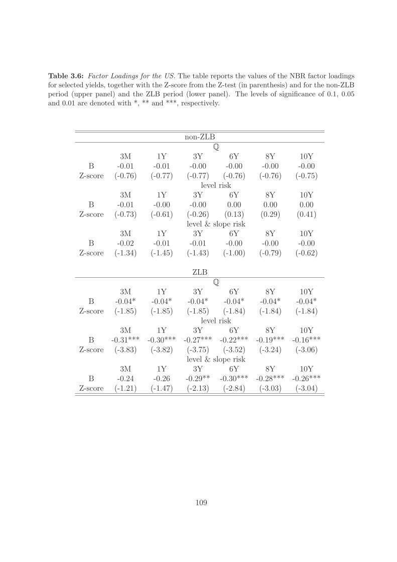
Table 3.6: Factor Loadings for the US. The table reports the values of the NBR factor loadingsfor selected yields, together with the Z-score from the Z-test (in parenthesis) and for the non-ZLBperiod (upper panel) and the ZLB period (lower panel). The levels of significance of 0.1, 0.05and 0.01 are denoted with *, ** and ***, respectively.

non-ZLBQ

3M 1Y 3Y 6Y 8Y 10YB -0.01 -0.01 -0.00 -0.00 -0.00 -0.00

Z-score (-0.76) (-0.77) (-0.77) (-0.76) (-0.76) (-0.75)level risk

3M 1Y 3Y 6Y 8Y 10YB -0.01 -0.00 -0.00 0.00 0.00 0.00

Z-score (-0.73) (-0.61) (-0.26) (0.13) (0.29) (0.41)level & slope risk

3M 1Y 3Y 6Y 8Y 10YB -0.02 -0.01 -0.01 -0.00 -0.00 -0.00

Z-score (-1.34) (-1.45) (-1.43) (-1.00) (-0.79) (-0.62)

ZLBQ

3M 1Y 3Y 6Y 8Y 10YB -0.04* -0.04* -0.04* -0.04* -0.04* -0.04*


3M 1Y 3Y 6Y 8Y 10YB -0.31*** -0.30*** -0.27*** -0.22*** -0.19*** -0.16***

Z-score (-3.83) (-3.82) (-3.75) (-3.52) (-3.24) (-3.06)level & slope risk

3M 1Y 3Y 6Y 8Y 10YB -0.24 -0.26 -0.29** -0.30*** -0.28*** -0.26***

Z-score (-1.21) (-1.47) (-2.13) (-2.84) (-3.03) (-3.04)

109

Table 3.7: Factor Loadings for Switzerland. The table reports the values of the reserves factorloadings for the pre-ZLB period (upper panel) and ZLB period (lower panel) for selected yields,together with the Z-score from the Z-test (in parenthesis). The levels of significance of 0.1, 0.05and 0.01 are denoted with *, ** and ***, respectively.

pre-ZLBQ

3M 1Y 3Y 6Y 8Y 10YB -0.00 -0.00 -0.00 -0.00 -0.00 -0.00


3M 1Y 3Y 6Y 8Y 10YB 0.01 0.01 0.01 0.00 0.00 -0.00

Z-score (1.56) (1.50) (1.28) (0.77) (0.21) (-0.67)level & slope risk

3M 1Y 3Y 6Y 8Y 10YB -0.01 -0.01 -0.01 -0.01 -0.01 -0.01

Z-score (-0.24) (-0.26) (-0.36) (-0.70) (-1.01) (-1.33)

ZLBQ

3M 1Y 3Y 6Y 8Y 10YB -0.04*** -0.04*** -0.04*** -0.03*** -0.03*** -0.03***

Z-score -(2.64) -(2.65) -(2.66) -(2.67) -(2.68) -(2.68)level risk

3M 1Y 3Y 6Y 8Y 10YB -0.08*** -0.08*** -0.08*** -0.08*** -0.07*** -0.07***

Z-score -(2.59) -(2.63) -(2.75) -(2.90) -(2.96) -(2.97)level & slope risk

3M 1Y 3Y 6Y 8Y 10YB 0.03 0.00 -0.04 -0.06* -0.07** -0.07**

Z-score (0.40) (0.08) -(0.82) -(1.84) -(2.16) -(2.26)

110

Figure 3.1: Interest Rates and Central Bank Reserves in the US. The term structure of interestrates (left scale) is plotted for the non-ZLB (upper panel) and ZLB-period (lower panel), togetherwith the NBR (right scale).

111

Figure 3.2: Interest Rates and Central Bank Reserves in Switzerland. The term structure ofinterest rates (left scale) is plotted for the non-ZLB (upper panel) and ZLB-period (lower panel),together with the total sight deposits (right scale).

112

Figure 3.3: Estimated Posteriors for the US. The Figure illustrates the estimated posteriordensities for all the parameters of the model used to estimate the QE effect in US data.

113

Figure 3.4: Latent Factors for US Data. The Figure plots the evolution of the three estimatedlatent factors in the period away from the ZLB (upper panel) and at the ZLB (lower panel) forUS data.

114

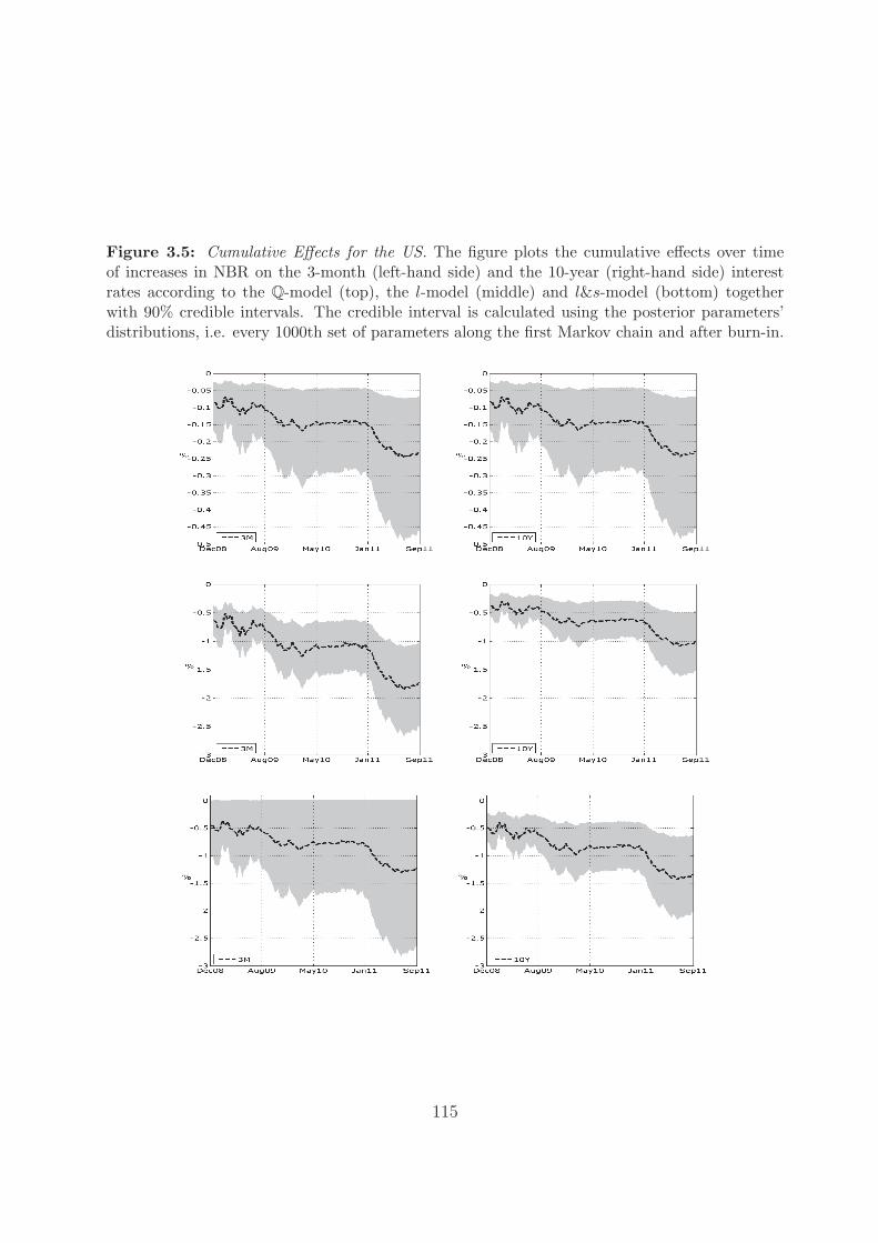
Figure 3.5: Cumulative Effects for the US. The figure plots the cumulative effects over timeof increases in NBR on the 3-month (left-hand side) and the 10-year (right-hand side) interestrates according to the Q-model (top), the l-model (middle) and l&s-model (bottom) togetherwith 90% credible intervals. The credible interval is calculated using the posterior parameters’distributions, i.e. every 1000th set of parameters along the first Markov chain and after burn-in.

115

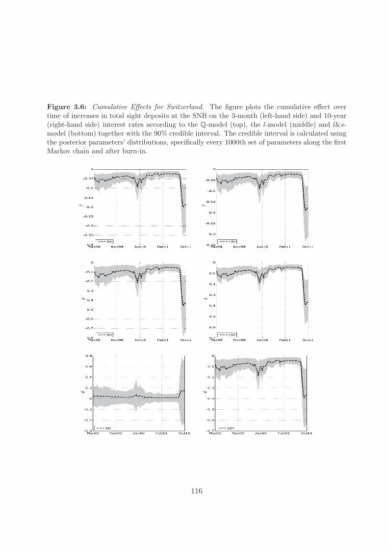
Figure 3.6: Cumulative Effects for Switzerland. The figure plots the cumulative effect overtime of increases in total sight deposits at the SNB on the 3-month (left-hand side) and 10-year(right-hand side) interest rates according to the Q-model (top), the l-model (middle) and l&s-model (bottom) together with the 90% credible interval. The credible interval is calculated usingthe posterior parameters’ distributions, specifically every 1000th set of parameters along the firstMarkov chain and after burn-in.

116

Figure 3.7: Separating Supply and Liquidity Effects in US Data. The upper panel depicts weeklydata of NBR and the Federal Reserves’ holdings of Treasury securities with more than one year tomaturity. The lower panel draws the cumulative liquidity effect by multiplying the difference inthe changes of reserves and Treasury holdings by the NBR factor loadings of the 10-year maturityas estimated in Table 3.6. The solid black line refers to the most conservative estimate at theZLB which results under the Q-measure, the dashed red line to the most optimistic estimate thatresults from the l & s model.

117

Bibliography

Andersson, Fredrik N. G., “Long Run Inflation Indicators - Why the ECB got it Right,”

Technical Report 2008.

Andres, Javier J., David Lopez-Salido, and Edward Nelson, “Tobin’s Imperfect

Asset Substitution in Optimizing General Equilibrium,” Journal of International Money

and Finance, 2004, 36 (5), 665–90.

Andrews, Donald W. K., “Tests for Parameter Instability and Structural Change with

Unknown Change Point: A Corrigendum,” Econometrica, 2003, 71 (1).

and Werner Ploberger, “Optimal Tests when a Nuisance Parameter is Present Only

Under the Alternative,” Econometrica, 1994, 62 (6).

Ang, Andrew and Geert Bekaert, “Regime Switches in Interest Rates,” Journal of

Business & Economic Statistics, 2002, 20 (2), pp. 163–182.

and Monika Piazzesi, “A no-arbitrage vector autoregression of term structure dy-

namics with macroeconomic and latent variables,” Journal of Monetary Economics, May

2003, 50 (4), 745–787.

, Geert Bekaert, and Min Wei, “The Term Structure of Real Rates and Expected

Inflation,” The Journal of Finance, 2008, 63 (2), 797–849.

, Sen Dong, and Monika Piazzesi, “No-Arbitrage Taylor Rules,” NBER Working

Papers 13448, National Bureau of Economic Research, Inc September 2007.

Assenmacher-Wesche, Katrin and Stefan Gerlach, “Money at Low Frequencies,”

Journal of the European Economic Association, 2007, 5 (2-3), 534–542.

119

and , “Understanding the Link between Money Growth and Inflation in the Euro

Area,” in David P. Cobham, ed., The Travails of the Eurozone, Palgrave Macmillan,

Basingstoke, 2007, pp. 10–39.

and , “Interpreting euro area inflation at high and low frequencies,” European Eco-

nomic Review, 2008, 52 (6), 964–986.

and , “Money growth, output gaps and inflation at low and high frequency: Spectral

estimates for Switzerland,” Journal of Economic Dynamics and Control, 2008, 32 (2),

411–435.

Backus, David K. and Jonathan H. Wright, “Cracking the Conundrum,” Brookings

Papers on Economic Activity, 2007, 1, 293–329.

Batini, Nicoletta and Edward Nelson, “The Lag from Monetary Policy Actions to

Inflation: Friedman Revisited,” International Finance, 2001, 4 (3), 381–400.

Bauer, Gregory H. and Antonio Diez de los Rios, “An International Dynamic Term

Structure Model with Economic Restrictions and Unspanned Risks,” Working Paper,

2011.

Bauer, Michael D., “Term Premia and the News,” Federal Reserve Bank of San Francisco

Working Paper Series, 2011.

and Glenn D. Rudebusch, “The signaling channel for Federal Reserve bond pur-

chases,” Technical Report 2011.

and , “The Signaling Channel for Federal Reserve Bond Purchases,” Federal Reserve

Bank of San Francisco Working Paper Series, 2011-21.

Baxter, Marianne and Robert G. King, “Measuring Business Cycles: Approximate

Band-Pass Filters For Economic Time Series,” The Review of Economics and Statistics,

1999, 81 (4), 575–593.

Beck, Gunter and Volker Wieland, “Money in Monetary Policy Design under Un-

certainty: The Two-Pillar Phillips Curve versus ECB-Style Cross-Checking,” CEPR

Discussion Papers 6098, C.E.P.R. Discussion Papers 2007.

120

and , “Money in monetary policy design: Monetary cross-checking in the New-

Keynesian model,” CEPR Discussion Papers 7518, C.E.P.R. Discussion Papers October

2009.

Beck, Guenter W. and Volker Wieland, “Central bank misperceptions and the role

of money in interest-rate rules,” Journal of Monetary Economics, 2008, 55, 1–17.

Benati, Luca, “Long Run Evidence on Money Growth and Inflation,” Working Paper

Series 1027, European Central Bank 2009.

Berger, Helge and Par Osterholm, “Does Money Growth Granger-Cause Inflation in

the Euro Area? Evidence from Out-of-Sample Forecasts Using Bayesian VARs,” IMF

Working Papers 08/53, International Monetary Fund 2008.

Bernanke, Ben S and Alan S Blinder, “The Federal Funds Rate and the Channels of

Monetary Transmission,” American Economic Review, 1992, 82 (4), 901–21.

Bernanke, Ben S. and Ilian Mihov, “The liquidity effect and long-run neutrality,”

Carnegie-Rochester Conference Series on Public Policy, 1998, 49 (1), 149–194.

Calvet, Laurent E., Aldai Fisher, and Liuren Wu, “Dimension - Invariant Dynamic

Term Structures,” Working Paper, 2010.

Campbell, John Y., Andrew Wen-Chuan Lo, and A. Craig MacKinlay, “The

econometrics of financial markets,” Princeton University Press, 1997, 2.

Canova, Fabio and Tobias Menz, “Does money matter in shaping domestic business

cycles? An international investigation,” Working Paper, Department of Economics,

University Pompeu Fabra, Barcelona 2009.

Carpenter, Seth and Selva Demiralp, “The Liquidity Effect in the Federal Funds

Market: Evidence at the Monthly Frequency,” Journal of Money, Credit and Banking,

2008, 40 (1), 1–24.

Chen, Ren-Raw and Louis Scott, “Multi-Factor Cox-Ingersoll-Ross Models of the Term

Structure: Estimates and Tests from a Kalman Filter Model,” Journal of Real Estate

Finance and Economics, Vol. 27, No. 2, 1993.

121

Chib, Siddhartha, “Markov chain Monte Carlo methods: computation and inference,”

in J.J. Heckman and E.E. Leamer, eds., Handbook of Econometrics, Vol. 5 of Handbook

of Econometrics, Elsevier, January 2001, chapter 57, pp. 3569–3649.

and Bakhodir Ergashev, “Analysis of Multifactor Affine Yield Curve Models,” Jour-

nal of the American Statistical Association, 2009, 104 (488), 1324–1337.

Chow, Gregory C., “Tests of Equality Between Sets of Coefficients in Two Linear Re-

gressions,” Econometrica, 1960, 28 (3), pp. 591–605.

Christensen, Jens H. E. and Glenn D. Rudebusch, “The Response of Government

Yields to Central Bank Purchases of Long-Term Bonds,” Working Paper preliminary,

Federal Reserve Bank of San Francisco 2012.

Christiano, Lawrence J and Martin Eichenbaum, “Identification and the Liquidity

Effects of a Monetary Shock,” Cuikerman et.al (eds), Political Economy, Growth and

the Business Cycle, 1992.

and , “Liquidity Effects and the Monetary Transmission Mechanism,” American

Economic Review, 1992, 82 (2), 346–53.

and , “Liquidity Effects, Monetary Policy, and the Business Cycle,” Journal of

Money, Credit and Banking, 1995, 27 (4), 1113–36.

Cochrane, John H, “The Return of the Liquidity Effect: A Study of the Short-run

Relation between Money Growth and Interest Rates,” Journal of Business & Economic

Statistics, 1989, 7 (1), 75–83.

Cochrane, John H. and Monika Piazzesi, “Decomposing the Yield Curve,” SSRN

eLibrary, 2009.

Corbae, Dean, Sam Ouliaris, and Peter C.B. Phillips, “Band Spectral Regression

with Trending Data,” Cowles Foundation Discussion Papers 1163, Cowles Foundation,

Yale University 1997.

Dahlquist, Magnus and Henrik Hasseltoft, “International Bond Risk Premia,” SSRN

eLibrary, 2011.

122

Dai, Qiang and Kenneth J. Singleton, “Specification Analysis of Affine Term Structure

Models,” The Journal of Finance, 2000, 55 (5), 1943–1978.

, , and Wei Yang, “Regime Shifts in a Dynamic Term Structure Model of U.S.

Treasury Bond Yields,” Review of Financial Studies, 2007, 20 (5), 1669–1706.

D’Amico, Stefania and Thomas B. King, “Flow and stock effects of large-scale Trea-

sury purchases,” Finance and Economics Discussion Series 2010-52, Board of Governors

of the Federal Reserve System (U.S.) 2010.

D’Amico, Stefania and Thomas B King, “Flow and Stock Effects of the Large Scale

Treasury Purchases,” Paper presented at Conference on Monetary Policy at the Zero

Lower Bound, held at the Federal Reserve Bank of San Fransisco, 25 February 2011,

2011, 0 (0), 75–83.

Diebold, Francis X. and Canlin Li, “Forecasting the term structure of government

bond yields,” Journal of Econometrics, February 2006, 130 (2), 337–364.

Dotsey, Michael and Peter Ireland, “Liquidity Effects and Transactions Technologies,”

Journal of Money, Credit and Banking, 1995, 27 (4), 1441–57.

Duffee, Greg, “Sharpe ratios in term structure models,” Economics Working Paper

Archive 575, The Johns Hopkins University,Department of Economics April 2010.

Duffee, Gregory R., “Term Premia and Interest Rate Forecasts in Affine Models,” Jour-

nal of Finance, 02 2002, 57 (1), 405–443.

Duffie, Darrell, “Special Repo Rates,” The Journal of Finance, 1996, 51 (2), pp. 493–526.

and Rui Kan, “A Yield-Factor Model Of Interest Rates,” Mathematical Finance, 1996,

6 (4), 379–406.

Dwyer, Gerald P. and R.W. Hafer, “Is money irrelevant?,” Review, Federal Reserve

Bank of St. Louis 1988.

Engle, Robert F, “Band Spectrum Regression,” International Economic Review, 1974,

15 (1), 1–11.

123

, “Testing Price Equations for Stability across Spectral Frequency Bands,” Econometrica,

1978, 46 (4), 869–81.

Favara, Giovanni and Paolo Giordani, “Reconsidering the Role of Money for Output,

Prices and Interest Rates,” Journal of Monetary Economics, 2009, 56 (3), 419–430.

Favero, Carlo A, Linlin Niu, and Luca Sala, “Term Structure Forecasting: No-

Arbitrage Restrictions vs Large Information Set,” CEPR Discussion Papers 6206,

C.E.P.R. Discussion Papers March 2007.

Fitzgerald, Terry J., “Money growth and inflation: how long is the long run?,” Economic

Commentary, 1999, (Aug 1).

Friedman, Milton, “Factors Affecting the Level of Interest Rates,” Proceedings of the

1968 Conference on Savings and Residential Financing, 1968, pp. 10–27.

, “Have Monetary Policies Failed?,” American Economic Review, 1972, 62 (2), 11–18.

Gagnon, Joseph, Matthew Raskin, Julie Remache, and Brian Sack, “Large-scale

asset purchases by the Federal Reserve: did they work?,” Staff Reports 441, Federal

Reserve Bank of New York 2010.

, , , and , “Large-scale asset purchases by the Federal Reserve: did they work?,”

Economic Policy Review, 2011.

Gerlach-Kristen, Petra, “A Two-Pillar Phillips Curve for Switzerland,” Swiss Journal

of Economics and Statistics (SJES), 2007, 143 (IV), 425–448.

Gerlach, Stefan, “The ECB’s Two Pillars,” CEPR Discussion Papers 3689, C.E.P.R.

Discussion Papers 2003.

Geweke, John, “The Superneutrality of Money in the United States: An Interpretation

of the Evidence,” Econometrica, 1986, 54 (1), 1–21.

Giese, Julia V., “Level, Slope, Curvature: Characterising the Yield Curve in a Cointe-

grated VAR Model,” Economics - The Open-Access, Open-Assessment E-Journal, 2008,

2 (28), 1–20.

124

Gilks, W.R, “Full Conditional Distributions in Gilks W.R., Richardson S. and Spiegel-

halter D.J. Markov Chain Monte Carlo in Practice,” Chapman and Hall, 1996.

Goodfriend, Marvin and Robert G. King, “The incredible Volcker disinflation,”

Journal of Monetary Economics, 2005, 52 (5), 981–1015.

Gordon, David B and Eric M Leeper, “The Dynamic Impacts of Monetary Policy:

An Exercise in Tentative Identification,” Journal of Political Economy, 1994, 102 (6),

1228–47.

Granger, C W J, “Investigating Causal Relations by Econometric Models and Cross-

Spectral Methods,” Econometrica, 1969, 37 (3), 424–38.

Grauwe, Paul De and Magdalena Polan, “Is Inflation Always and Everywhere a

Monetary Phenomenon?,” Scandinavian Journal of Economics, 2005, 107 (2), 239–259.

Greene, William H., Econometric Analysis, 2nd ed., Prentice Hall, 1993.

Greenwood, Robin and Dimitri Vayanos, “Bond Supply and Excess Bond Returns,”

Working Paper, Harvard Business School 2010.

Grossman, Sanford and Laurence Weiss, “A Transactions-Based Model of the Mon-

etary Transmission Mechanism,” American Economic Review, 1983, 73 (5), 871–80.

Gurkaynak, Refet S., Brian Sack, and Jonathan H. Wright, “The U.S. Treasury

yield curve: 1961 to the present,” Journal of Monetary Economics, November 2007, 54

(8), 2291–2304.

Hagedorn, Marcus, “Money, Interest Rates and Strong Liquidity Effects,” Working

Paper, University of Zurich 2009.

Hamilton, James D, “Measuring the Liquidity Effect,” American Economic Review,

1997, 87 (1), 80–97.

Hamilton, James D. and Jing (Cynthia) Wu, “Identification and Estimation of

Affine-Term-Structure Models,” 2010.

125

and , “The Effectiveness of Alternative Monetary Policy Tools in a Zero Lower Bound

Environment,” Working Paper, University of California, San Diego 2010.

Harrison, J. Michael and David M. Kreps, “Martingales and arbitrage in multiperiod

securities markets,” Journal of Economic Theory, June 1979, 20 (3), 381–408.

Hull, John C., Options, Futures, and Other Derivatives with Derivagem CD (7th Edi-

tion), 7 ed., Prentice Hall, May 2008.

Jardet, Caroline, Alain Monfort, and Fulvio Pegoraro, “No-Arbitrage Near-

Cointegrated VAR(p) Term Structure Models, Term Premia and GDP Growth,” SSRN

eLibrary, 2011.

Jordan, Bradford D. and Susan D. Jordan, “Special Repo Rates: An Empirical

Analysis,” The Journal of Finance, 1997, 52 (5), pp. 2051–2072.

Joslin, Scott, Kenneth J. Singleton, and Haoxiang Zhu, “A New Perspective on

Gaussian Dynamic Term Structure Models,” Review of Financial Studies, 2011.

, Marcel Priebsch, and Kenneth J. Singleton, “Risk Premiums in Dynamic Term

Structure Models with Unspanned Macro Risks,” 2010.

Jr., Robert E. Lucas, “Two Illustrations of the Quantity Theory of Money,” American

Economic Review, 1980, 70 (5), 1005–14.

, “A Journey from Theory to Practice.,” Panel Discussion: Colloquium in Honor of Ot-

mar Issing, presented at ECB colloquium Monetary Policy, Frankfurt: European Central

Bank 2006.

Judson, Ruth A. and Elizabeth Klee, “Whither the liquidity effect: The impact of

Federal Reserve open market operations in recent years,” Journal of Macroeconomics,

2010, 32 (3), 713–731.

Kaufmann, Sylvia and Peter Kugler, “Does Money Matter For Inflation In The Euro

Area?,” Contemporary Economic Policy, 2008, 26 (4), 590–606.

King, Robert G. and Mark W. Watson, “Money, Prices, Interest Rates and the

Business Cycle,” The Review of Economics and Statistics, 1996, 78 (1), 35–53.

126

and , “Testing long-run neutrality,” Economic Quarterly, 1997, (Sum), 69–101.

Kirchgassner, Gebhard, “Zum Kausalzusammenhang zwischen Geldmenge und Sozial-

produkt: Ubersicht uber neuere Arbeiten und empirische Ergebnisse fur die Bundesre-

publik Deutschland, 1960-1979,” European Journal of Political Economy, 1985, 1 (3),

399–456.

and Jurgen Wolters, “The Role of Monetary Aggregates in the Policy Analysis of

the Swiss National Bank,” Working Paper Series 2009-30, Department of Economics,

University of St. Gallen 2009.

Koop, Gary, “Bayesian Econometrics,,” John Wiley and Sons Ltd, 2003.

Krishnamurthy, Arvind and Annette Vissing-Jorgensen, “The Effects of Quanti-

tative Easing on Interest Rates,” Technical Report 2011.

Krogstrup, Signe, Samuel Reynard, and Barbara Sutter, “Liquidity Effects of

Quantitative Easing on Long-Term Interest Rates,” Working Paper forthcoming, Swiss

National Bank 2012.

Kuttner, Kenneth, “Can Central Banks Target Bond Prices?,” NBER Working Papers

12454, National Bureau of Economic Research, Inc 2006.

Litterman, Robert and J Scheinkman, “Common factors affecting bond returns,” The

Journal of Fixed Income, 1991, 1 (1), 54–61.

Lucas, Robert Jr., “Liquidity and interest rates,” Journal of Economic Theory, 1990,

50 (2), 237–264.

Lynch, Scott M., Introduction to Applied Bayesian Statistics and Estimation for Social

Scientists, 7 ed., Springer Science+Business Media, 2007.

McCallum, Bennett T., “On Low-Frequency Estimates of "Long-Run" Re-

lationships in Macro- economics,” NBER Working Papers 1162, National Bureau of

Economic Research, Inc 1984.

127

Mikkelsen, Peter, “MCMC Based Estimation of Term Structure Models,” Finance Work-

ing Papers 01-7, University of Aarhus, Aarhus School of Business, Department of Busi-

ness Studies May 2001.

Neely, Christopher J., “The large scale asset purchases had large international effects,”

Working Papers 2010-018, Federal Reserve Bank of St. Louis 2010.

Nelson, Edward, “The future of monetary aggregates in monetary policy analysis,” Jour-

nal of Monetary Economics, 2003, 50 (5), 1029–1059.

, “Why Money Growth Determines Inflation in the Long Run: Answering the Woodford

Critique,” Journal of Money, Credit and Banking, 2008, 40 (8), 1791–1814.

Nicoletti Altimari, Sergio, “Does money lead inflation in the euro area?,” Technical

Report 2001.

Pagan, Adrian R. and John C. Robertson, “Resolving the liquidity effect,” Proceed-

ings, 1995.

Phillips, Alban William Housego, “The Relation Between Unemployment and the

Rate of Change of Money Wage Rates in the United Kingdom, 1861-1957,” Economica,

1958, 25 (2), 283–299.

Phillips, P. C. B., “The Structural Estimation of a Stochastic Differential Equation

System,” Econometrica, 1972, 40 (6), pp. 1021–1041.

Reynard, Samuel, “Money and the Great Disinflation,” Working Papers 2006-7, Swiss

National Bank 2006.

, “Maintaining low inflation: Money, interest rates, and policy stance,” Journal of Mon-

etary Economics, 2007, 54 (5), 1441–1471.

Sargent, Thomas and Paolo Surico, “Monetary policies and low-frequency manifesta-

tions of the quantity theory,” Discussion Papers 26, Monetary Policy Committee Unit,

Bank of England 2008.

and , “Two Illustrations of the Quantity Theory of Money: Breakdowns adn Re-

vivals,” Working paper, New York University 2009.

128

Sims, Christopher A., “Interpreting the macroeconomic time series facts : The effects

of monetary policy,” European Economic Review, 1992, 36 (5), 975–1000.

, “Inflation expectations, uncertainty, the Phillips curve, and monetary policy,” Confer-

ence Series 53, Federal Reserve Bank of Boston 2009.

Skarr, Doug, “Understanding Interest Rate Swaps: Math and Pricing,” California Debt

and Investment Advisory Commission, 2010.

Soderlind, Paul, “Reaction of Swiss Term Premia to Monetary Policy Surprises,” Swiss

Journal of Economics and Statistics (SJES), March 2010, 146 (I), 385–404.

Thoma, Mark A, “The Effects of Money Growth on Inflation and Interest Rates across

Spectral Frequency Bands,” Journal of Money, Credit and Banking, 1994, 26 (2), 218–31.

Thornton, Daniel L., “The daily and policy-relevant liquidity effects,” Working Paper

Series 984, European Central Bank 2008.

, “The daily and policy-relevant liquidity effects,” Working Paper Series 984, European

Central Bank December 2008.

Tobin, James, “Liquidity Preference as Behaviour towards Risk,” Journal of Interna-

tional Money and Finance, 1958, 25 (2).

Trecroci, Carmine and Juan Luis Vega-Croissier, “The information content of M3

for future inflation,” Working Paper Series 33, European Central Bank 2000.

Vayanos, Dimitri and Jean-Luc Vila, “A Preferred-Habitat Model of the Term Struc-

ture of Interest Rates,” NBER Working Papers 15487, National Bureau of Economic

Research, Inc 2009.

Whiteman, Charles H, “Lucas on the Quantity Theory: Hypothesis Testing without

Theory,” American Economic Review, 1984, 74 (4), 742–49.

Woodford, Michael, “Does a ’Two-Pillar Phillips Curve’ Justify a Two-Pillar Monetary

Policy Strategy?,” CEPR Discussion Papers 6447, C.E.P.R. Discussion Papers 2007.

, “How Important is Money in the Conduct of Monetary Policy?,” Journal of Money,

Credit and Banking, 2008, 40, 1561–98.

129

Curriculum Vitae

Personal Details

Name Barbara Caroline Sutter

Date of Birth 27 February 1980

Citizenship Swiss (Ormalingen and Winterthur)

Education

2008 - 2013 University of St. Gallen, Switzerland

PhD in Economics and Finance

2008 Study Center Gerzensee, Switzerland

Program for Beginning Doctoral Students in Economics


Master of Arts in Quantitative Economics and Finance, M.A. HSG


Bachelor of Arts in Economics, B.A. HSG

Professional Experience

2011 - Swiss National Bank, Zurich, Switzerland

Money Market and Foreign Exchange

2007 - 2010 Swiss National Bank, Zurich, Switzerland

Economic Research

2005 UBS AG, Zurich, Switzerland

Wealth Management International, Active Portfolio Supervision

2004 UBS AG, Zurich, Switzerland

Wealth Management International, Product & Sales Management BCG

130

Three Essays in Monetary Economics - Liquidity and its Effects on

Documents

Transcript of Three Essays in Monetary Economics - Liquidity and its Effects on