ESSAYS IN MONETARY POLICY CONDUCTION AND ITS EFFECTIVENESS:

MONETARY POLICY RULES, PROBABILITY FORECASTING, CENTRAL BANK

ACCOUNTABILITY, AND THE SACRIFICE RATIO

A Dissertation

by

GABRIEL CASILLAS OLVERA

Submitted to the Office of Graduate Studies of Texas A&M University

in partial fulfillment of the requirements for the degree of

DOCTOR OF PHILOSOPHY

August 2004

Major Subject: Agricultural Economics

ESSAYS IN MONETARY POLICY CONDUCTION AND ITS EFFECTIVENESS:

MONETARY POLICY RULES, PROBABILITY FORECASTING, CENTRAL BANK

ACCOUNTABILITY, AND THE SACRIFICE RATIO

A Dissertation

by

GABRIEL CASILLAS OLVERA

Submitted to Texas A&M University

in partial fulfillment of the requirements for the degree of

DOCTOR OF PHILOSOPHY

Approved as to style and content by:

David A. Bessler Leonardo Auernheimer (Chair of Committee) (Member)

John B. Penson, Jr. David J. Leatham (Member) (Member)

Paul D. Mitchell A. Gene Nelson (Member) (Head of Department)

August 2004

Major Subject: Agricultural Economics

iii

ABSTRACT

Essays in Monetary Policy Conduction and Its Effectiveness:

Monetary Policy Rules, Probability Forecasting, Central Bank

Accountability, and the Sacrifice Ratio. (August 2004)

Gabriel Casillas Olvera,

B.A., Instituto Tecnológico y de Estudios Superiores de Monterrey,

Campus Estado de Mexico

Chair of Advisory Committee: Dr. David A. Bessler

Monetary policy has been given either too many positive attributes or, in contrast,

only economy-disturbing features. Central banks must take into account a wide variety

of factors to achieve a proper characterization of modern economies for the optimal

implementation of monetary policy. Such is the case of central bank accountability and

monetary policy effectiveness. The objective of this dissertation is to examine these two

concerns relevant to the current macroeconomic debate. The analyses are carried out

using an innovative set of tools to extract presumably important information from

historical data of selected macroeconomic indicators.

This dissertation consists of three essays. The first essay explores the causality

between the elements of the “celebrated” Taylor rule, using a Structural Vector

Autoregression approach on US data. Directed acyclical graph techniques and Bayesian

search models are used to identify the contemporaneous causal structure in the

construction of impulse-response functions. Further analysis is performed by

iv

evaluating the implications of performing standard innovation-accounting procedures,

derived from a Structural Vector Autoregression on interest rates, inflation, and

unemployment. This is examined whenever a causal structure is imposed vs. when it is

observed. We find that the interest rate causes inflation and unemployment. This

suggests that the Fed has not followed a Taylor rule in any of the two periods under

study. This result differs significantly to the case when the causal structure is imposed.

The second essay presents an incentive-compatible approach based on proper

scoring rules to evaluate density forecasts in order to reduce the central banks’

accountability problem. Our results indicate that the surveyed forecasters have done a

“better” job than the Monetary Policy Committee (MPC).

The third essay analyzes the causal structure of the factors that are presumed to

influence the effectiveness of monetary policy, represented by the sacrifice ratio.

Directed acyclical graph methods are used to identify the causal flow between such

determinants and the sacrifice ratio. We find evidence that, while wage rigidities and

central bank independence are the two major determinants of the sacrifice ratio, the

degree of openness has no direct effect on the sacrifice ratio.

v

To my beloved wife Teresa, the source of my inspiration

vi

ACKNOWLEDGEMENTS

The beginning of my journey to pursue a Ph.D. was a very intricate one. My father

passed away after a two-year battle against prostate cancer at the early age of 52, five

days later, I was taking my first graduate course at A&M. He encouraged me until his

last breath to continue with my plans, regardless of the outcome. So I did.

This unfortunate event left me lacking my primary source of professional guidance.

I am extremely thankful that I was embraced by Professors David Bessler, David

Leatham, Leonardo Auernheimer, John Penson, and Paul Mitchell, members of my

graduate advisory committee. I cannot thank them enough for their friendship,

continuous motivation, as well as for their most valuable critical appraisal, and

insightful conversations during these four years.

From making me derive a four-period-ahead, three-variable impulse-response

function by hand, or asking me to provide with a sensible explanation for an odd step

in a demonstration of an adverse-selection problem with continuum of types, up to

requesting me to derive an equation characterizing the relative price of a tree in terms

of bananas, my committee has helped to achieve a better understanding of the use, and

application of the major tools used in modern economics. Fortunately, they have always

spiced these hard technical questions with humorous stories. For example, I will never

forget Dr. Bessler’s story about the pit barbecue he and Jon Brandt prepared for their

fellow students and professors during his days at Davis, as well as the state-contingent

McDonald’s option that they never exercised. On the other hand, they have always

vii

gone further and tried to transmit deeper philosophical ideas emphasizing the role of

economics as a social science. I want to express my deepest appreciation and eternal

gratitude to Professor David Bessler who was the most directly involved in the

development of this dissertation. I am also especially grateful to Dr. Mitchell for his

support and guidance during the presentations of research papers in several seminars

and meetings. I am also indebted to Dr. Penson and Dr. Capps for sharing words of

wisdom and sustained encouragement. Special thanks to Dr. Leatham for making me

believe again in myself, thanks for your trust and encouragement.

I benefited greatly from enlightening conversations with Professors John Nichols,

Allan Love, George Davis, Rich Woodward, Rudy Nayga, Ron Griffin, James

Richardson, Vicky Salin, Dror Goldberg, William Neilson, and Thomas Jeitschko. I also

want to thank Professor Gene Nelson for his wise counseling, practical ideas, and for

trusting me with the development of the graduate website. I am pleased to have served

as teaching assistant for Professors John Siebert and John Park. It was a very rewarding

experience. I learned a lot from their excellent teaching styles. Many thanks to René

Ochoa for his advice and interesting conversations. Special thanks to Vicky Heard for

her support, and unconditional and effective help whenever it was needed. I also want

to acknowledge the helpful assistance that I got from Norma Pantoja, Lindsey Nelson,

Adrienne Blaskey, Ruth Hicks, Stella Garcia, Cindy Fazzino, and Michelle Zinn.

Graduate school would not have been so bearable if it were not for my fellow Aggie

Ph.D. students and colleagues (Whoop!) Ernesto Perusquía, Pablo Sherwell, Gustavo

Sánchez, Luis Ribera, Iván Borja, César Corredor, Grant Pittman, Michael Lau, Matt

viii

Stockton, Debbie Rubbas, Hwa-Nyeon Kim, Karla Rossette, Levan Elbakidze, Tanveer

Butt, Jim Sartwell, Hae-Sun Park, Jin-Woon Kim, Moon-Soo Park, David Magaña,

Andrés Silva, Matt Schupbach, Juan Carlos Serrano, Ivan Tasic, Ahmad Al-Waked,

Dandan Lui, and Ahmet Caliskan. Grant and Hwa: Thanks for putting up with such a

“chatter-box” office mate along these years.

Thanks to Javier, Maritza, and Javi Reyes for their support along these years.

Gustavo y Mayren contributed a great deal to continuously keeping my spirit up

against frustration. I am extremely grateful to Pablo González and Marcela Perticara for

their emotional support at the beginning of graduate school, a difficult period of my

life. They embraced me almost like a son, providing me with great Argentinean-style

food, academic help, words of encouragement, and great friendship. Special thanks to

Ernesto Perusquía, my faithful friend and companion through the battles to conquer the

Ph.D. Thanks also for the enlightening conversations either about economics or college

football. I owe a deep debt of gratitude to Pablo Sherwell for providing the much-

needed housing during my last year full of journeys between Dallas and College

Station. Thanks for his unconditional friendship, golf lessons, and unending discussions

about the political economy in Mexico.

My father, an engineer who did not hold any degree in economics, planted the first

seed of my interest in this interesting discipline by letting me read his old copy of

Samuelson’s Economics book. After speaking to me so much about how wonderful and

important economics was, I could not understand why he was surprised the day I told

him I wanted to be an economist. Thanks Dad.

ix

I am greatly indebted to my professors at ITESM. I am especially grateful with

Marcela Villegas, Benjamin García, Miguel Mayorga, Luis Quintana and Gerardo

Dubcovsky. Thanks also to Emilio Alvarado and Pepe Duarte for their guidance.

Many of the early ideas in this dissertation were born during my tenure at Banco de

México, thanks to my fruitful conversations with Ignacio Peralta, Chemanel Carrera,

Javier Duclaud, David Margolin, Ricardo Medina, Luis Mario Hernández, Alfonso

Guerra, Alejandro Aguilar, Rafa Figueroa, Emilio Lozoya, Juan Cristóbal Gil, and

Alfredo Sordo. Special thanks to Javier Duclaud for his advice and support.

I gratefully acknowledge the financial support from CONACYT and Banco de

México, as well for the scholarships, fellowships, and assistantships from the

Department of Agricultural Economics and Texas A&M University.

Thanks to my friends Omar González, Carlos Guisa, Javier Sosa, Paty Rivas,

Mauricio Diaz, Tomás Alcántara, José Luis and Katia Torres Landa, Luis Flores, Richard

Ramirez-Webster, Charlie Cortes, Alejandro Martínez, Checho Morales, Toño Cortés,

and Guillermo Aviña for their strong support.

My deepest appreciation and sincere love will always be felt for my family in

Mexico. I am eternally thankful with my mother and my sister for their unconditional

physical and emotional support and endless caring.

Tere: Thanks for understanding the endless nights that I had to spend working on

preparing my qualifying and prelim exams, my dissertation proposal, this dissertation,

and my final defense. Thanks for your patience and your wise counseling. I will never

find the words to thank you enough. Muchas gracias mi amor.

x

TABLE OF CONTENTS

CHAPTER Page

I INTRODUCTION ............................................................................................................ 1 II STRUCTURAL VECTOR AUTOREGRESSIONS AND THE TAYLOR RULE: IMPOSING VS. OBSERVING A CAUSAL STRUCTURE ........................... 13

A. Introduction.......................................................................................... 13 B. The Taylor Rule.................................................................................... 17

1. Derivation of the Taylor Rule from a Model of Optimizing Agents ................................................ 19 2. An Empirical Approach of the Taylor Rule: Structural Vector Autoregressions ....................................... 26 3. Stock and Watson’s Model and Replication ....................... 29

C. Probabilistic Approach to Empirical Causality ............................... 31 1. Directed Acyclical Graphs and the PC Algorithm............. 32 2. Calculus of Interventions....................................................... 37

D. Results ................................................................................................... 38 E. Conclusions........................................................................................... 42

III PROBABILITY FORECASTING AND CENTRAL BANK ACCOUNTABILITY..................................................................... 44

A. Introduction.......................................................................................... 44 B. Transparency, Accountability, and Forecast Evaluation ............... 52

1. Central Banks Tradition of Secrecy, Problems, and Proposed Solutions....................................... 52 2. Recent Increased Central Bank Transparency .................... 55 3. Forecasting as a Reputation-Building Mechanism ............ 58 4. Density Forecasts in Monetary Policy.................................. 59

C. Probability Forecasting ....................................................................... 60 1. Prequential Analysis .............................................................. 60 2. Probability Forecast Evaluation............................................ 61 3. Empirical Assessment of Calibration................................... 61 4. Scoring Rules ........................................................................... 63 5. The Quadratic Probability Rule and the Brier Score.......... 64 6. Yates’ Decomposition of the Brier Score ............................. 67 7. The Multiple-Event Brier Score............................................. 72

xi

CHAPTER Page

8. Which Score Shall We Calculate? The Probability Score or the Mean Probability Score?................................... 75 9. Hypothesis Testing for the Brier Score ................................ 75

D. Bank of England Fan Charts Evaluation .......................................... 78

1. Bank of England Inflation Report......................................... 78 2. Probability Scores, Brier Scores and Yates’ Partitions of the Density Forecasts of the UK..................... 80 3. Are the MPC and the “Other” Forecasters’ Brier Scores

Significantly Different? .......................................................... 86 E. Conclusions........................................................................................... 87

IV WHAT CAUSES THE SACRIFICE RATIO? .............................................................. 93

A. Introduction.......................................................................................... 93 B. Calculating the Sacrifice Ratios.......................................................... 98

1. The Sacrifice Ratio .................................................................. 98 2. Identifying Disinflation Periods and the Measurement of the Output Gap ......................... 102 3. Estimates of the Sacrifice Ratio ........................................... 104

C. Determinants of the Sacrifice Ratio ................................................. 108 1. Traditional Factors................................................................ 109 2. Structural Factors.................................................................. 111 3. Institutional Factors.............................................................. 112

D. Empirically-Based Causal Structure................................................ 115 1. Directed Acyclical Graphs................................................... 117 2. PC Algorithm ........................................................................ 118

E. What Causes the Sacrifice Ratio?..................................................... 121 1. Imposed Causal Structure on Ball’s Seminal Analyses.................................................................. 122 2. Results .................................................................................... 124

F. Conclusions......................................................................................... 130

V CONCLUSIONS........................................................................................................... 133

REFERENCES…………………………………………………………………………….. 138 APPENDIX A TABLES………. ........................................................................................ 155 APPENDIX B FIGURES………........................................................................................ 171

xii

Page

APPENDIX C PROGRAMS………. ................................................................................ 185

VITA……………….. ........................................................................................................... 204

1

CHAPTER I!

INTRODUCTION

Central banks have never been more powerful than now. Monetary policy has become the central tool of macroeconomic stabilization. ― Richard Layard (1996), pg. ix

Traditionally economists have divided macroeconomic policy into two lines of

attack: fiscal and monetary policy. It is usually monetary and not fiscal policy that can

be adjusted in a timely fashion to respond to macroeconomic events. Fiscal policy is

typically subject to slow and uncertain legislative processes. However, the usefulness of

monetary policy has been challenged as a stabilization mechanism. Uncertainties

emerging from the degree of influence of monetary policy on output and inflation, as

well as the possible adverse shocks the economy may face sets up an array of difficult

intricacies that the central bank must overcome. In addition, the monetary authority

must deal with the complexity of the lag structure of the monetary policy transmission

mechanism, the choice of the relevant instruments and targets, and modeling issues,

such as the characterization of the monetary authority’s objective function1. There is a

large part of the modern macroeconomic literature, namely Real Business-Cycle theory

(RBC), that presumes that monetary policy has no effect on real variables and, as a

! This dissertation follows the style and format of the American Economic Review.

1 Usually the models use Kydland-Prescott (1977), and Barro-Gordon (1983)-style loss functions to represent the central banker’s utility function. As Blinder (1998) points out, central bankers have to generate their own welfare function build upon their legal mandate, due to the political authorities’ lack of precision when giving instructions to the central bank.

2

result, money should not been included in their models. However, several empirical

studies, such as Sims (1992), conclude that monetary policy innovations account for

substantial effects on real output and that recessions have been frequently preceded by

unexpected rises in interest rates. Moreover, they claim that it is impossible for RBC-

style models to explain a major extent of the variations on the observed business cycles.

Therefore, carrying out analysis on the conduction of monetary policy is a

tremendously important research task to achieve an objective assessment on its

effectiveness.

Aiming to minimize the already diminishing gap2 between the academic and the

policymakers’ view of monetary policy, the objective of this dissertation is to develop

and apply tools to examine and improve the implementation of monetary policy and its

effectiveness. A description of the proposed topics under study follows.

Policy lags (Friedman, 1969a, and Phelps, 1967) and rational expectations (Lucas,

1981b) led to the conclusion that there was no such thing as a long-run trade-off

between output and inflation. This implies that monetary policy cannot affect output or

unemployment in the long-run. But it can have an effect on inflation. In other words,

activist monetary policy just disrupts the economy yielding a high inflation outcome.

This “old” version of the “rules vs. discretion” debate left the use of any kind of

discretionary rules out of the conduction of monetary policy. However, this is not the

end of the story, this dispute evolved into a new version.

2 McCallum (1999) asserts that the split between academic and policymaker views on monetary policy conduction has been reduced in recent years.

3

The existence of a “time-consistency” problem –first noticed in the monetary

literature by Auernheimer (1974)- also called “inflation bias”, is defined as the

excessively high equilibrium inflation generated by the credibility problem that comes

along when the central banks exercise their ability to temporarily boost the economy

(Kydland and Prescott, 1977, Barro and Gordon, 1983), plays an important role in the

more recent version of the rules vs. discretion debate (Persson and Tabellini, 1999). This

“modern” version led some researchers to reconsider a less restrictive class of rules,

motivating a plethora of research on monetary policy rules. This is the first topic

addressed in this dissertation.

McCallum (1988) and Taylor (1993) pioneered the development of these dynamic

monetary policy rules. The latter, proposed another set of rules where the instrumental

interest rate changes in response to any deviation of the inflation rate from a desired

target value and to the output gap, defined as the difference between the real and

potential GDP. The former suggested a family of rules that stands for an automatic

reaction of the monetary base growth rate to any deviation of the nominal GDP growth

rate from a desired target value. On the other side of the debate, while some authors,

such as Gordon (1985), Meltzer (1987), and Hall and Mankiw (1994), support the

money-base rule with nominal GDP targeting, Goodhart (1994), Fuhrer and Moore

(1995) and Bryant, et al. (1993) argue that McCallum-type of rules has undesirable

stabilization features, and that interest rate rules with are operationally better.

Conversely, recent research has demonstrated that both rules are practically equivalent

when the monetary base velocity is a stable function of the interest rate (Razzak, 2001).

4

Another debate that has become known is the robustness of the monetary policy

rules under “model uncertainty”. In other words, how these rules perform when they

are built upon different models. This, of course, is due to the well-known ambiguities

that surface when it comes down to knowing the “true” structure of the economy

(Levin, Wieland, and Williams, 1999). They conclude that the required information to

set the interest rate efficiently is summarized by inflation, output gap, and interest rates.

This indicates that a reduced-form vector autoregression (VAR) analysis on these

variables could be a well suited tool for assessing this topic. For a monetary policy rule

to be effective it has to be based upon a model that reflects accurately the economy.

Consequently, it becomes crucial to analyze the causal structure of the variables that

have been recognized as key factors that interact themselves to form the monetary

transmission mechanism. Structural vector autoregressions (SVAR) were chosen to

achieve this endeavor.

Unfortunately, “activist” monetary policy rules impose certain undesirable

restrictions to the policymaker, impairing them to optimally respond to adverse shocks.

Hall and Mankiw (1994) argue that trying to maintain one variable under strict control,

could bring volatility to other variables. As a result, there is near consensus that these

rules should not be used as systematic mechanisms to act to stabilize the economy3.

Taylor (1993) recommends using these rules as guidelines for policymaking decisions.

This inherent restrictiveness comes from the fact that a commitment to a simple

instrument rule is not considered as an appropriate description of current monetary

3 Actually, Taylor (1999) and Feldstein (1999b) maintain that policymakers should work with a reasonable portfolio of policy rules.

5

policy (Svensson, 2003). That is why, in order to find an “intermediate” monetary

scheme between discretion and either fully mechanical or “activist” rules, institutional

arguments emerged, such as central bank independence (CBI) and targeting

frameworks, such as Inflation Targeting (IT). This constrained flexibility is desirable

since despite monetary policy cannot systematically affect unemployment and output

in the long-run, it might aid to stabilize inflation and unemployment around their mean

market-determined levels (Fischer, 1977).

CBI is described as the assignment of monetary policy to a central banker whose

decisions cannot be rejected ex post by the policymaker (Lippi, 1999). Herrendorf and

Neumann (1999) claim that a politically-detached independent central bank exhibits

less incentives to care about the government’s reelection chances reducing the

possibilities of using monetary policy to create surprise inflation4. But independence

could be associated with a greater degree of “conservativeness” in the Rogoff (1985)

sense. In other words, greater independence may imply less-active stabilization policies

and, therefore, higher output variance. This suggests that the gains of having an

independent central bank depend on the extent of the trade-off between the inflationary

bias and the variance of the policy targets, as a result, in addition to CBI, stability of

policy targets is desired to overcome the time-inconsistency problem (Lippi, 1999). In

other words, CBI and targeting regimes are not viewed as substitutes, but

complements.

4 The monetary policy credibility issues have been criticized because, in reality, usually policymakers do not try to create unexpected inflation to surprise the private sector. But these criticisms miss the point that, in equilibrium, despite the monetary authority’s wish to reduce the inflation rate, it abstains from doing it because the disinflationary policy could turn into a recession, due to its lack of credibility.

6

A mechanism that could be in the middle between full-discretion and restriction is

Inflation Targeting (IT). But still, even an inflation targeting regime, being a constrained

discretion regime country could show an inflation bias if there is no incentives to

achieve the target. In other words, the ex-post measure that the IT regime provides as

inflation and the target could still not fully get rid of the inflation bias since there could

be moral hazard. The central banker in charge can always provide a somewhat “good”

explanation of why she could not achieve the target. Hence, additional to the inflation

targeting regime, these points raise the question of what can be done to eliminate the

moral hazard that feeds the credibility problem.

One way to deal with this problem is to hire a conservative central banker as Rogoff

(1985) suggest. Lamentably, it is not easy to find out whether a central banker is

sufficiently conservative or not (Barro, 1986). In that case, another asymmetric

information problem surfaces: adverse selection at the time of deciding who to appoint

as central banker. Yet, the moral hazard problem remains. Alternatively, another

approach by Walsh (1995a), and Persson and Tabellini (1993) is to write a contract

between the government (principal) and the central banker (agent) as an incentive-

compatible mechanism to achieve the desired results. In other words, build a gifts-

punishments scheme between the congress and the central bank. On this issue,

Garfinkel and Oh (1993) assert that legislation punishing the monetary authority by

reducing her salary of the central bank’s budget, if she deviates from the target could be

used to enforce the regime. Unfortunately, the intrinsic complexity in modeling the

government’s preferences causes serious difficulties to build a totally applicable

7

contract. Blinder (1998) criticizes this approach by stating that the principal, by having a

reelection period ahead, could have more incentives to have an inflation bias than the

agent, who is not supposed to be concern about the political election process. Another

point of disapproval is that the perhaps the salary is not a good motivator for the

central banker to do her job since she is already giving up salary for not being working

in the private sector. Another mechanism that has been talked about in the literature is

reputation. Reputation seems like a good initiative once we now how to make the

central bank accountable. Canzoneri (1985) proves that reputation as an inflation-bias

elimination framework does not work in the presence of private information (such as

their inflation forecast). Full disclosure of the inflation-forecast by the central bank is

not intended to pass on information to the private sector, but to be accountable of her

actions. As Blinder (1998) humorously points out, reputation is not unlike pregnancy –

either you have it or not-, therefore, inflation targeting should be accompanied by an

inflation-forecast evaluation method, the second topic treated in this dissertation.

Since the Timbergen (1952) and Theil (1961) framework of macroeconometric single-

equation estimation, up to Chris Sims (1980) and others, forecasting has been a very

important issue not only for academic economists, but to influence a policy debate

(Barrel, 2001). For the forecast to work as a reputation building mechanism in the

Canzoneri (1985) sense, it should neither be private information nor a disturbance

element. It needs to satisfy two conditions: (i). Have full disclosure of the forecast and

how the forecasting methods, and (ii.) The forecast has to be a “good” forecast (Winkler,

1986). By this, we mean that, on one hand it must reflect the banks’ true beliefs. In other

8

words, when outcomes are uncertain, planning must be based on forecasts quite often

on forecasts submitted by others. Naturally, the planner wishes to ensure that these

forecasts are prepare honestly and with an appropriate degree of care (Osband, 1989).

On the other hand, it must be an accurate forecast as well. So not only should the

central banker provide their true beliefs about their future expectations on inflation

(and, if there is the case, on GDP as well), but also exert their best effort to provide a

“good” forecast. If we want to really take into account the uncertainties that surrounds

the forecast, it is recommended to be in probabilistic form (Samuelson, 1965, Bessler

and Moore, 1979).

Why distribution forecasting? Svensson (2003) points out, inflation-forecast

targeting in a point-forecast sense only works under three assumptions: (i) Quadratic

loss function, (ii) linear transmission mechanism, and (iii) additive uncertainty. The

first assumption is reasonable and widely used, Kydland-Prescott (1977), Barro and

Gordon (1983), as well as supported by more recent research led by Blinder (1998),

Svensson, (2001, 2002), and others. The second assumption, linear transmission

mechanism is a quite strong assumption, since it means that the future target variables

depend on the current state of the economy and the instrument in a linear fashion and

that is not usually the fact (Svensson, 2003). The third assumption, if there is

uncertainty of policy multipliers. If assumptions (ii) and (iii) fail, then the certainty

9

equivalence paradigm does not hold5, then, distribution forecast is needed to account

for unbalanced risks.

Once we are convinced that probability forecasting is a much better way to

approach macroeconomic problems (Bessler and Moore, 1979, Tay and Wallis, 2000,

Granger, 2001), evaluation issues become a topic of concern (de Finetti, 1974, Winkler,

1986), such as calibration (Bunn, 1984, Kling and Bessler, 1989). But there are other

considerations such as how close the forecast is from the realized values (Yates, 1982,

Bessler and Ruffley, 2003). We use the Brier Score (Brier, 1950) and the Yates’

Decomposition (Yates, 1982). The Brier score is a proper scoring rule. It has been both

theoretically and experimentally demonstrated to be an incentive-compatible

mechanism (Nelson and Bessler, 1989). The third aspect is to compare, i.e. to make

competitions between the central bank and other forecasters. A more general rationale

to use probabilistic forecasting evaluation criteria is the fact that currently, the

economists’ duty is to habitually explore economic systems in which agents interact in

complex probabilistic environments (Chari, 1998). A final remark is that probabilistic

forecast is possible. The Bank of England publishes their forecasts, as well as other

surveyed forecasters’ numbers, on a regular basis in their quarterly Inflation Report, since

1996. We use Bank of England’s and other forecasters inflation and output growth rate

probabilistic forecasts, to illustrate the formidable and practical applications of the Brier

5 Although there are sophisticated models that deal with parameter uncertainty using optimal control models with learning mechanisms, Blinder (1998) points out that the intrinsic complexity of these methods have not caught both academics’ and policymakers’ attention.

10

score and its Yates’ partition as a building reputation mechanism to reduce the inflation

bias in an inflation target regime.

We turn now to the third essay in this dissertation. Monetary policy would not seem

to be so important if we could not assess monetary policy’s effectiveness. A way to

measure monetary policy effectiveness is by looking at the sacrifice ratio. Lawrence Ball

(1994) studies methods to calculate the ratios. Questions related to what determines the

sacrifice ratio, or what causes the sacrifice ratio, remain unanswered. Is it wage rigidity?

Is it the monetary policy regime, such as inflation targeting? This is the third point of

focus of the dissertation.

There is almost consensus that disinflation policies generate output losses (Gordon,

1982, Gordon and King, 1982, and Romer and Romer, 1989). But what is the cost of

those monetary policy tightening policies in the real world? In an effort to measure

those costs and their possible determinants, several authors have estimated the sacrifice

ratio, generally defined as the quotient between the output gap and the percent change

in inflation, and have drawn simple scatter diagrams or calculated simple correlations

between the ratio and the variables that are assumed to most likely have an impact on

it.

According to Ball’s seminal paper (Ball, 1994), the factors that may determine

the magnitude of the sacrifice ratios could be the length of the disinflation period, the

initial inflation, the degree o wage rigidity –among others-. Later on, also Ball asks if

inflation targets matters. Bernanke, et al. (1999) perform a study on the sacrifice ratios.

The theoretical argument on why a country adopting an inflation targeting regime

11

should have a smaller sacrifice ratio is that IT provides a framework that constraints the

monetary authority and minimizes its incentives to exhibit an opportunistic behavior –

also called inflation bias- and this increases credibility and the public moderates their

inflations expectations in a quicker fashion.

The purpose if to use the same methodology used on the Taylor rule analysis,

namely, Directed Acyclical Graph theory and the PC algorithm to identify an

empirically-based causal structure of the main determinants of the sacrifice ratio.

The objective of this dissertation is to examine these three concerns relevant to the

current macroeconomic debate. The analyses are carried out using an innovative set of

tools to extract presumably important information from historical data of simple

macroeconomic indicators, to examine and improve the implementation of monetary

policy and its effectiveness.

The interlinkages of inflation with agriculture have been well documented. The

impacts of inflation on the agricultural lending institutions have been studied by

Klinefelter, Penson, and Fraser, (1980) as well as by LaDue and Leatham, (1984) and

Barnett, Bessler and Thompson (1983). Also, monetary policy decisions affect the

exchange rates, as well as prices and price volatility. Moreover, in the case of the

forecasts of main macroeconomic indicators, it has been shown that they have an

important effect in the agricultural sector (Penson and Gardner, 1988). On the other

hand, a study on how the disinflationary policies have affected the agricultural income

in different countries can be a subject of study as well.

12

This dissertation consists of three essays. The first essay (chapter II) examines the

causality between the elements of the celebrated Taylor rule, using Structural Vector

Autoregressions on US data for the period between the first quarter of 1960 and the

fourth quarter of 2000. Directed acyclical graph techniques and Bayesian search models

are used to identify the contemporaneous causal structure in the construction of

impulse-response functions.

The second essay (chapter III) presents a probabilistic approach for inflation forecast

evaluation that aims to integrate the academic version of “inflation bias” reduction

mechanisms with some practical implementation issues. This is illustrated by applying

the Brier probabilistic forecast evaluation criterion on data of the UK.

The third essay (chapter IV) analyzes the causal structure of the factors that are

presumed to influence the sacrifice ratio on panel data of eleven OECD countries using

Directed Acyclical Graphs to identify the causal flow of the sacrifice ratio and its

determinants. Chapter V summarizes the results of this research and renders the

concluding remarks.

13

CHAPTER II

STRUCTURAL VECTOR AUTOREGRESSIONS AND THE TAYLOR RULE:

IMPOSING VS. OBSERVING A CAUSAL STRUCTURE

There are for man only two principles available for a mental grasp of reality, namely, those of teleology and causality. What cannot be brought under either of these categories is absolutely hidden to the human mind. An event not open to an interpretation by one of these two principles is for man inconceivable and mysterious. ― Ludwig von Mises (1949), p. 24.

A. Introduction

While the “old” version of the rules vs. discretion debate6 led by Friedman (1969a),

Phelps (1967), and Lucas (1981a) left out the use of any kind of discretionary rules on

the conduction of monetary policy, its “modern” version7 (Kydland and Prescott, 1977

and Barro and Gordon, 1983) led some researchers to reconsider a less restrictive class

of rules. This motivated a plethora of research on monetary policy rules pioneered by

McCallum (1988) and Taylor (1993). The former suggested a family of rules that stands

6 Because of policy lags (Friedman, 1969a, and Phelps, 1967) and rational expectations (Lucas, 1981b), the consensus dictate that there is not such a thing as long-run trade-off between output and inflation, implying that in the long-run, monetary policy cannot affect output or unemployment, but inflation only. In other words, activist monetary policy just disrupts the economy yielding a high inflation outcome.

7 The existence of a “time-consistency” problem, first noticed in the monetary literature by Auernheimer (1974), or “inflation bias”, is defined as the excessively high equilibrium inflation generated by the credibility problem that comes along when the central banks exercise their ability to temporarily boost the economy (Kydland and Prescott, 1977, Barro and Gordon, 1983), plays an important role in the more recent version of the rules vs. discretion debate (Persson and Tabellini, 1999).

14

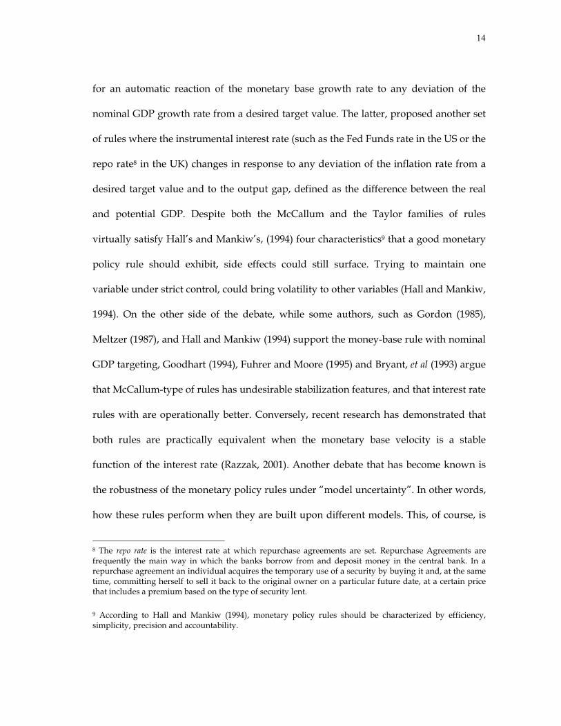
for an automatic reaction of the monetary base growth rate to any deviation of the

nominal GDP growth rate from a desired target value. The latter, proposed another set

of rules where the instrumental interest rate (such as the Fed Funds rate in the US or the

repo rate8 in the UK) changes in response to any deviation of the inflation rate from a

desired target value and to the output gap, defined as the difference between the real

and potential GDP. Despite both the McCallum and the Taylor families of rules

virtually satisfy Hall’s and Mankiw’s, (1994) four characteristics9 that a good monetary

policy rule should exhibit, side effects could still surface. Trying to maintain one

variable under strict control, could bring volatility to other variables (Hall and Mankiw,

1994). On the other side of the debate, while some authors, such as Gordon (1985),

Meltzer (1987), and Hall and Mankiw (1994) support the money-base rule with nominal

GDP targeting, Goodhart (1994), Fuhrer and Moore (1995) and Bryant, et al (1993) argue

that McCallum-type of rules has undesirable stabilization features, and that interest rate

rules with are operationally better. Conversely, recent research has demonstrated that

both rules are practically equivalent when the monetary base velocity is a stable

function of the interest rate (Razzak, 2001). Another debate that has become known is

the robustness of the monetary policy rules under “model uncertainty”. In other words,

how these rules perform when they are built upon different models. This, of course, is

8 The repo rate is the interest rate at which repurchase agreements are set. Repurchase Agreements are frequently the main way in which the banks borrow from and deposit money in the central bank. In a repurchase agreement an individual acquires the temporary use of a security by buying it and, at the same time, committing herself to sell it back to the original owner on a particular future date, at a certain price that includes a premium based on the type of security lent.

9 According to Hall and Mankiw (1994), monetary policy rules should be characterized by efficiency, simplicity, precision and accountability.

15

due to the well-known ambiguities that surface when it comes down to knowing the

“true” structure of the economy (Levin, Wieland, and Williams, 1999). They conclude

that the required information to set the interest rate efficiently is summarized by

inflation, output gap, and interest rates.

This indicates that a reduced-form vector autoregression (VAR) analysis on these

variables could be a well suited tool for assessing this topic. And it is precisely this

specific raison d'être that triggered our interest on this first topic of our discussion. For a

monetary policy rule to be effective it has to be based upon a model that reflects

accurately the economy. Consequently, it becomes crucial to analyze the causal

structure of the variables that have been recognized as key factors that interact

themselves to form the monetary transmission mechanism. Structural vector

autoregressions (SVAR) have been chosen to achieve this endeavor.

Sims’ seminal paper (1980), dictated the general norm on “modern”

macroeconometric modeling estimating vector autoregressions (VAR) from data on the

major macroeconomic variables. Within Sims’ modeling framework, a descriptive

mechanism called impulse-response function was also introduced to analyze the

reaction of each variable in the model to a shock in each equation of the system. Aiming

to be able to show the dynamic patterns for each variable, these shocks must satisfy

orthogonally conditions. In order to achieve this desired provision, a Choleski

decomposition was used. Cooley and LeRoy (1984) noticed that by applying this

factorization method, one might have imposed some undesirable restrictions on the

model in terms of causal behavior.

16

In response to this claim, Blanchard and Quah (1989), Blanchard (1989), and Stock

and Watson (2001) –among others- have approached the problem by building means to

impose structure to the so-called “atheoretical VARs”. Bernanke (1986)10 handled the

problem using an alternative decomposition that allows for nonlinear restrictions on the

off-diagonal elements of what they call pattern matrix.

However, only theoretical restrictions have been imposed in VAR analyses of

monetary policy rules, and it would be interesting not only to know if the data supports

the major theories on how monetary policy affects the economy, but also to evaluate the

usefulness of monetary policy rules in the implementation of monetary policy.

If we want to test if this is the empirical underlying causal structure, the Directed

Graph paradigm is able to analyze how the variables are causally related in

contemporaneous time. In order to perform this task, since the data is dynamically

related, it would be we useful (almost imperative) to “pre-filter” the data using a vector

autoregression. Then we would be able to use the PC algorithm on the residuals before

actually run the impulse-response functions. We decided to use Stock and Watson’s

(2001) VAR as a starting point since it was inspired by the Taylor rule.

As in Bessler and Lee (2002) and Bessler and Yang (2003), this is achieved by

identifying a causal structure of the estimated contemporaneous innovations derived

from an unrestricted VAR, and then restricting it using a Bernanke ordering (Bernanke,

1986, and Doan, 2000).

10 The focus here is on how Sims (1986), Bernanke (1986), and Blanchard (1989) theories influenced the causal ordering of the variables for the computation of the impulse-response functions and the forecast-error variance decomposition. For a more general treatment on structural VARs please see Amisano and Giannini (1997)

17

We want to answer the question if the US has (or has not) followed a Taylor-style

monetary policy rules in the period between first quarter of 1960 and the fourth quarter

of 2000. The other contribution of this paper is to analyze the consequences of analyzing

policy actions when a causal structure –namely the Taylor rule- is imposed, rather than

observing what the monetary authority has done.

The remainder of this chapter is divided in three sections. Section B portrays both

theoretical and empirical-based discussions about the Taylor rule. We describe the

directed acyclical graph models of causality in section C. Section D shows our results.

Finally, we reserved the last part for conclusions.

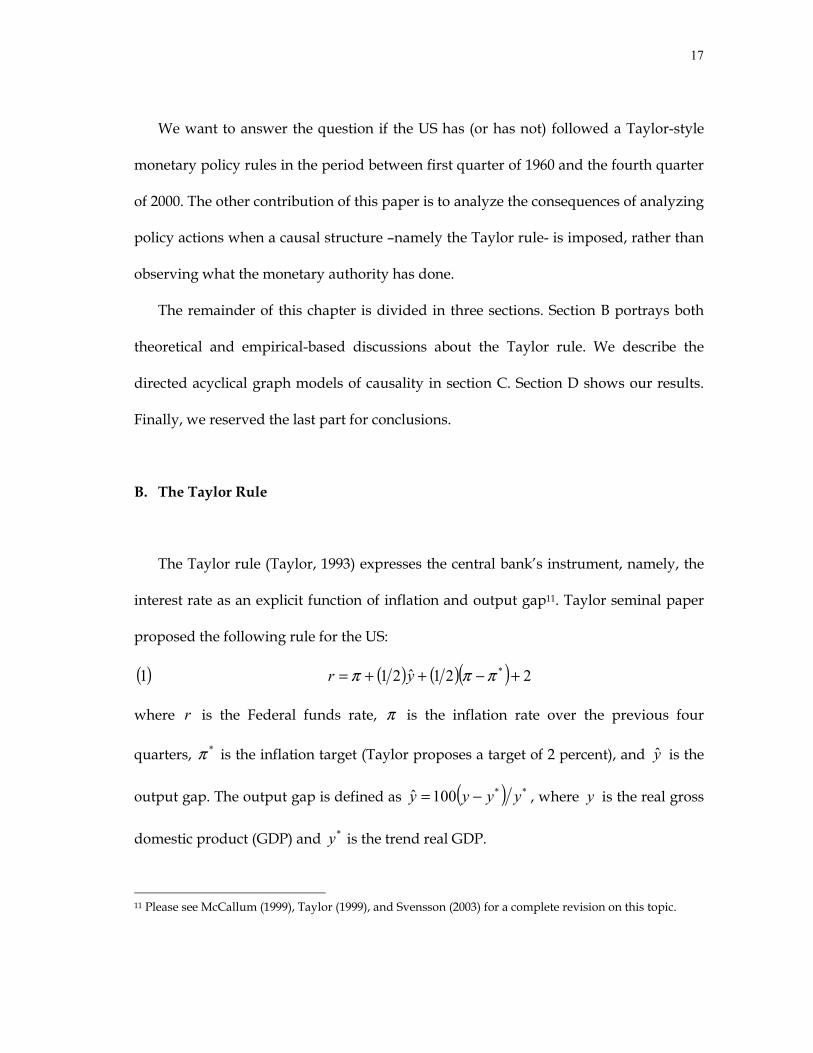
B. The Taylor Rule

The Taylor rule (Taylor, 1993) expresses the central bank’s instrument, namely, the

interest rate as an explicit function of inflation and output gap11. Taylor seminal paper

proposed the following rule for the US:

( )1 ( ) ( )( ) 221ˆ21 * +−++= πππ yr

where r is the Federal funds rate, π is the inflation rate over the previous four

quarters, *π is the inflation target (Taylor proposes a target of 2 percent), and y is the

output gap. The output gap is defined as ( ) **100ˆ yyyy −= , where y is the real gross

domestic product (GDP) and *y is the trend real GDP.

11 Please see McCallum (1999), Taylor (1999), and Svensson (2003) for a complete revision on this topic.

18

Several empirical studies have emphasized the usefulness of instrument rules, such

as the Taylor rule, to describe the central banks’ behavior (Judd and Rudebusch, 1998;

Clarida, Galí and Gertler, 1998; Stock and Watson, 2001). Although Taylor’s original

exposition of the rule did not emerge from a rigorous theoretical model, Svensson

(1997) and Walsh (1998) show that the Taylor rule can be derived from the first-order

conditions from a model of optimizing agents, as a central bank’s reaction function.

Different models with their respective assumptions, structure, and monetary policy

channels of transmission can yield optimal policy rules similar to the Taylor rule. In this

regard, Levin, Wieland, and Williams (1999) examine the robustness of the Taylor rule

under model uncertainty. They conclude that the output gap, the four-quarter average

inflation rate, as well as lagged values of the Federal funds interest rate summarize

almost all the information relevant to describe the Fed’s behavior.

This section will provide a theoretical derivation of the Taylor rule, closely

following several sections of Walsh (1998), in order to emphasize the underlying

assumptions and model structure that this policy rule encompasses. Then, an empirical

treatment of the Taylor rule based on a structural vector autoregression (SVAR) is

described. Finally we present and replicate a vector autoregression (VAR) by Stock and

Watson (2001), inspired by the Taylor rule.

19

1. Derivation of the Taylor Rule from a Model of Optimizing Agents

Assume a Money-in-Utility-Function (MIU) model12 (Sidrauski, 1967, and Brock,

1974). A representative agent has to choose the streams of consumption, leisure, and

money balances to maximize her time-discounted preferences, subject to an

intertemporal budget constraint. Her preferences are represented by a constant relative

risk aversion (CRRA) utility function13, with money and consumption as arguments.

The budget constraint involves the stock of capital transition equation assuming a

Cobb-Douglas (Cobb and Douglas, 1928) neoclassical production function of labor and

capital.

The first-order conditions characterizing the steady-state of the MIU model can be

represented as a set of six expectational linear difference equations (production

function, a resource constraint, the relationship between marginal product of capital

and the expected rate of return, expected consumption equation, a Fisher equation,

relating the nominal and real interest rate, and a money supply equation), as shown by

Campbell (1994) and Uhlig (1995).

The model described above is still not useful for monetary policy analysis since it

exhibits the classical dichotomy (Modigliani, 1963; Patinkin, 1965). In other words, money

and monetary shocks do not affect real variables (output, consumption, and real

interest rate). his is because prices are assumed to be perfectly flexible. Walsh (1998, pp.

12 MIU models have been criticized on the grounds that they are a reduced-form model of a fully-specified model of transaction costs. Brock (1974) explains that money can yield utility by reducing transaction costs. However, Feenstra (1986) finds certain conditions under which a transaction cost model, such as a cash-in-advance model (Clower, 1967), and the MIU’s maximization problem are equivalent.

13 King, Plosser, and Rebelo (1988) claim that CRRA preferences are consistent with steady-state growth.

20

190-195) shows that the linear approximation of the MIU model (described above) can

incorporate a one-period nominal wage rigidity a la Taylor (1979, 1980). This is achieved

by assuming that the nominal wage rate, set to produce a real wage to clear the labor

market, is determined before the start of the period. Therefore, the real wage “target” is

a function of the expected price-level.

McCallum and Nelson (1997) treat capital as exogenous in the context of the

dynamic optimizing general equilibrium model described along this section. Capital

grows steadily at its trend rate. This precludes the model to examine issues concerning

capital accumulation. In addition, they assume that employment oscillates about a fixed

level due to an inelastic labor supply. Nevertheless, these simplifying assumptions help

to characterize an economy with four simple equations: aggregate supply, aggregate

demand, a money demand equation, and a Fisher equation.

The money demand equation is dropped from the system if we assume that the

central bank conducts monetary policy using the interest rate as the instrument. Thus,

the money demand is determined endogenously according to that equation. Monetary

policy shocks affect real variables directly via the interest rates.

The remaining system of three equations involves an aggregate demand, function of

expected output and interest rate, an aggregate supply, function of expected inflation

and expected output, and a Fisher equation connecting the nominal and the real interest

rate. The following part of the model is a variant of Walsh (1998, pp. 468-470).

With no capital and, consequently, no investment, output equals consumption (this

is the new aggregate resource constraint). Moreover, the introduction of Taylor’s

21

staggered price model defines prices as a constant return over wages. A price-

adjustment equation characterizes the adjustment of wages. Taylor also assumes that

the expected real average contract wage is an increasing function of the level of

economic activity. Hence, the equations relevant for the determination of output and

the price level are the aggregate demand, and the Taylor’s price-adjustment equation.

From here, we carefully follow Walsh (1998, pg. 468-470) model, with the exception

that we include just one lag in the aggregate demand equation. Walsh claims that if we

disregard the role of expected future inflation14, the US economy can be characterized

by the following three linear equations:

( )2 tttt uRyy +−= −− 1211 αα

( )3 tttt y ηγππ ++= −1

( )4 tttt ERr π111 −−− +=

where ty and 1−ty are the output at time t and one-period before, respectively, 1−tR is

the lagged value of the real interest rate, tπ and 1−tπ stand for the current and lagged

inflation rates, and 1−tr is the nominal interest rate at time 1−t . tu and tη are ... dii

random variables not known at time 1−t , with zero mean and variances uσ and ησ ,

and the α ’s and γ are positive parameters. In addition, 1α is assumed to be less than

unity.

14 Svensson (1997) proposes a variant of this model recognizing the role of expected inflation. His results are not dramatically different in terms of what we want to show, i.e. that the Taylor rule can be derived from a theoretical model of optimizing agents. This is backed by Fuhrer’s (1997) findings emphasizing the unimportance of the forward-looking expectations, based on an empirical study of the U.S.

22

Equations ( )2 , ( )3 , and ( )4 correspond to the aggregate demand, a price-

adjustment (or inflation) equation, and the Fisher equation, respectively.

Contrary to the utility maximization framework, the model above puts together

lagged variables that will help to capture the observed dynamics of the data, but it is

important to state this difference since it is a major source of criticisms such as

McCallum (1999) -among others- regarding the (still) ongoing debate among

economists about which is the “right” model upon which we should build the central

bank optimization representation.

Suppose that changes in the nominal interest rate ( tr ) affect inflation and output

with one-period lag15. The monetary authority sets the nominal interest rate r at time t

when ty and tπ are already known, and setting tr affects 1+tπ and 1+ty .

If we insert the inflation equations ( )3 and ( )4 (once we solved it for 1−tR ) into the

aggregate demand equation ( )2 , for period 1+t , we are left with:

( )5 ( ) 11211 +++ +−−−= ttttttt uyEryy γπαα

Taking expectations to both sides of equation ( )5 , conditional on information at

time t , and solving it recursively, yields the following expression:

( )6 ( )[ ] ( )[ ] 12121 11 ++ +−−−= ttttt uryy πααγα

For convenience, let’s define 11 ++ −≡ ttt uyθ . Therefore, we can re-express equations

( )2 and ( )3 for the period 1+t in the following way:

15 The Taylor rule in equation (1) is build upon quarterly data. A model dealing with more than one or two lagged periods can easily become intractable. Thus, along the same lines, this assumption can be thought as a model for annual data.

23

( )7 11 ++ += ttt uy θ

( )8 11 ++ ++= tttt υγθππ

where 111 +++ += ttt u ηγυ .

In the spirit of Kydland and Prescott (1977), assume that the central banker’s

preferences are represented by a quadratic loss function L , with the output gap

( )*yyt − , and the difference between the inflation rate and a target ( *π ) as arguments:

( )9 ( ) ( ) ( )( )2*1

2*1 2121 ππλ −+−= ++ ttt yyL

where 0>λ is the weight on output stabilization.

The policymaker’s optimization problem is choose tθ at each t so that she

minimizes the sum of discounted squared future deviations from the output and

inflation targets. Without loss of generality, assume that 0** == πy . Hence, the central

banker is faced with the following dynamic optimization problem:

( )10 ( )( ) 10,21min 221

<<+ ++∞

=∑ βπλβθ ititi

it yE

t

subject to the description of the economy, i.e. equations ( )7 and ( )8 . β is the standard

discount factor. Since the objective function is a real-valued continuous quadratic

function, the restrictions are linear and continuous, and the only state variable at time t

is tπ , the choice of θ in period zero will determine the level of inflation in period 1.

Moreover, the discount factor is bounded between zero and one, therefore we are able

to use Bellman’s principle of optimality (Bellman, 1957). Thus, using dynamic

programming, we can express ( )10 as a Bellman equation:

24

( )11 ( ) ( )( ) ( ){ }12

12

121min +++ ++≡ ttttt VyEVt

πβπλπθ

where ( )⋅V is the value function.

The first-order conditions are:

( )12 ( ) ( ) 012 =+++ +tttt t

VE πγβγπθγλ π

From the envelope theorem (Benveniste and Sheinkman, 1982), i.e. taking the derivative

of expression ( )11 with respect to tπ yields,

( )13 ( ) ( )1+++= ttttt ttVEV πβγθππ ππ

If we multiply both sides of expression ( )13 by γ , solve it for ( )1+tt tVE πγβ π ,

substitute it in equation ( )12 , and solve it for ( )ttV πγ π , we are left with:

( )14 ( ) tttV λθπγ π −=

Plugging expression ( )14 for one-period ahead, into equation ( )12 , and solving for

tθ yields,

( )15 ( )[ ] ( )[ ] tttt E πγλγθγλλβθ 21

2 +−+= +

Given that λ and γ are parameters, it is reasonable to assume that tθ is a linear

function of 1+tθ and tπ . Therefore, we can apply the method of undetermined coefficients16

to provide a conjectured general form of the solution and determine the specific

coefficients.

16 See Romer (2001), pp. 289-91, and Turnovsky (2000), pp. 89-91.

25

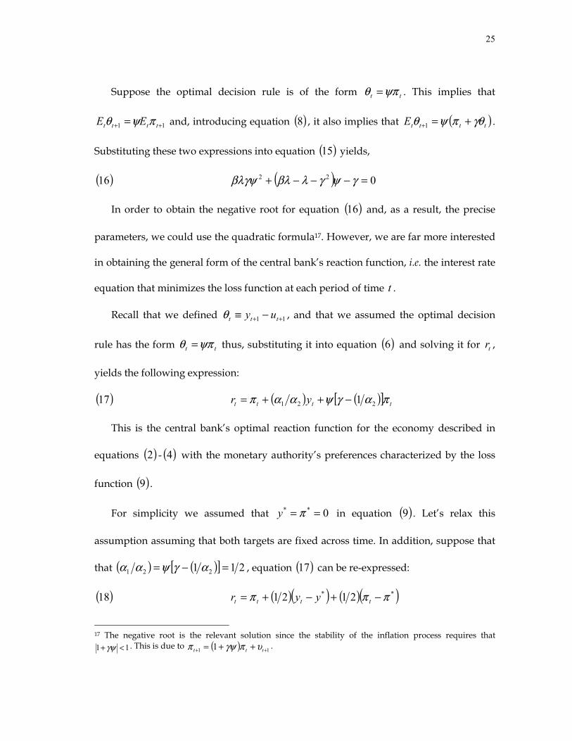
Suppose the optimal decision rule is of the form tt ψπθ = . This implies that

11 ++ = tttt EE πψθ and, introducing equation ( )8 , it also implies that ( )ttttE γθπψθ +=+1 .

Substituting these two expressions into equation ( )15 yields,

( )16 ( ) 022 =−−−+ γψγλβλβλγψ

In order to obtain the negative root for equation ( )16 and, as a result, the precise

parameters, we could use the quadratic formula17. However, we are far more interested

in obtaining the general form of the central bank’s reaction function, i.e. the interest rate

equation that minimizes the loss function at each period of time t .

Recall that we defined 11 ++ −≡ ttt uyθ , and that we assumed the optimal decision

rule has the form tt ψπθ = thus, substituting it into equation ( )6 and solving it for tr ,

yields the following expression:

( )17 ( ) ( )[ ] tttt yr παγψααπ 221 1−++=

This is the central bank’s optimal reaction function for the economy described in

equations ( )2 - ( )4 with the monetary authority’s preferences characterized by the loss

function ( )9 .

For simplicity we assumed that 0** == πy in equation ( )9 . Let’s relax this

assumption assuming that both targets are fixed across time. In addition, suppose that

that ( ) ( )[ ] 211 221 =−= αγψαα , equation ( )17 can be re-expressed:

( )18 ( )( ) ( )( )** 2121 πππ −+−+= tttt yyr

17 The negative root is the relevant solution since the stability of the inflation process requires that

11 <+γψ . This is due to ( ) 11 1 ++ ++= ttt υπγψπ .

26

Except for the lack of a number 2 adding to the right-hand side of the equation, this

equation is exactly the same as the equation ( )1 , i.e. the original version of the Taylor

rule (1993).

In order to obtain the same parameter numbers of Taylor (1993), the “deep”

parameters18 are 58.01 =α , 16.12 =α , and 26.0=γ for a discount factor of 96.0=β

(appropriate for annual data), and an output-stabilization weight of 1=λ , i.e. equal

weight on output and inflation. Therefore the original version of the Taylor rule entails

a strong response of spending to changes in interest rate ( 2α ) as well as inflation to

variability on output (γ ).

2. An Empirical Approach of the Taylor Rule: Structural Vector Autoregressions

We have painstakingly shown a way to derive the canonical form of the Taylor rule

from a model of optimizing agents. Now we turn to more practical concerns. In an

empirical research paper on robustness of monetary policy rules under model

uncertainty, Levin, Wieland, and Williams (1999) argue that the required information to

set the interest rate efficiently is summarized by inflation, output gap, and interest rates.

Therefore, from an empirical point of view, this suggests that a reduced-form vector

autoregression (VAR) analysis on these variables could be a well suited tool for

assessing this topic.

For a given vector of historical observations tX , a VAR can be expressed as:

18 These values are in line with Ball (1997).

27

( )19 tk

i itit XX ε+Φ+Φ= ∑ = −10

where tX and tε are 1×m random vectors, 0Φ is a vector of constants, and iΦ ,

ki ,,1 …= are matrices of coefficients with the appropriate dimensions. The vector of

disturbance terms, or innovations, tε is assumed to be i.i.d. with zero mean and a mm×

variance-covariance matrix εΣ . Innovations are assumed to be serially uncorrelated,

but contemporaneous correlations among elements of tε is allowed.

Sims’ seminal paper (1980), dictated the general norm on “modern”

macroeconometric modeling estimating vector autoregressions (VAR) from data on the

major macroeconomic variables. Within Sims’ modeling framework, a descriptive

mechanism called impulse-response function was also introduced to analyze the

reaction of each variable in the model to a shock in each equation of the system. Aiming

to be able to show the dynamic patterns for each variable, these shocks must satisfy

orthogonally conditions. In order to achieve this desired provision, a Choleski

decomposition was used. Cooley and LeRoy (1984) noticed that by applying this

factorization method, one might have imposed some undesirable restrictions on the

model in terms of causal behavior.

For a monetary policy rule to be effective it has to be based upon a model that

reflects accurately the economy. Consequently, it becomes crucial to analyze the causal

structure of the variables that have been recognized as key factors that interact

themselves to form the monetary transmission mechanism at a contemporaneous level.

28

In response to the already mentioned allegations by Cooley and Leroy (1984),

Blanchard and Quah (1989), Blanchard (1989), and Stock and Watson (2001) –among

others- have approached the problem by building means to impose structure to the so-

called “atheoretical VARs”, giving birth to the structural vector autoregressions

(SVARs). Bernanke (1986)19 handled the problem using an alternative decomposition

that allows for nonlinear restrictions on the off-diagonal elements of what they call

pattern matrix.

The observed innovations te are combinations of “structural” driving sources of

variation in the data. Following Amisano and Giannini’s (1997) K -model, based on

Bernanke (1986), these driving sources of variability are orthogonal and can be written

as:

( )20 tt Ke ε=

Assuming invertibility of the K matrix, identification is achieved if K , evaluated at

the “true” vector 0K , has full column rank of ( ) 21−mm . In other words, K will be

identified if we leave ( ) 21−mm free parameters in K (Amisano and Giannini, 1997,

pp. 35; Doan, 2000, pp. 8-10).

Innovation accounting procedures such as impulse-response functions and forecast-

error variance decomposition can be performed on the SVAR:

( )21 ∑ = − +Φ+Φ= k

i titit KXKKKX10 ε

19 The focus here is on how Sims (1986), Bernanke (1986), and Blanchard (1989) theories influenced the causal ordering of the variables for the computation of the impulse-response functions and the forecast-error variance decomposition. For a more general treatment on structural VARs please see Amisano and Giannini (1997)

29

However, theoretical restrictions have been imposed in VAR analyses of monetary

policy rules, and it would be interesting not only to know if the data supports the major

theories on how monetary policy affects the economy, but also to evaluate the

usefulness of monetary policy rules in the implementation of monetary policy. Even

Stock and Watson (2001, pg. 103) define a structural vector autoregression in the

following way: “A structural VAR uses economic theory to sort out the

contemporaneous links among the variables…”

Later in this paper, we will retrieve the causal structure from the set of data using a

fairly recent methodology called Directed Acyclical Graph (DAG) theory on causality,

developed by Pearl (2000) and Spirtes, Glymour and Scheines (1993, 2000) to assess the

usefulness of instrument-based (Taylor-style) monetary policy rules for the US

economy.

3. Stock and Watson’s Model and Replication

Stock and Watson (2001) present a three-variable VAR for the US macroeconomy

inspired by the Taylor rule for the 1960:I-2000:IV period. They pick output, inflation,

and unemployment as their set of variables20. The first two are practically “natural”

variables, but the third one differs from the original version of the Taylor rule (output

gap). Stock and Watson limit their explanation to note the difference between the

original Taylor rule and their approach (footnote no. 5, pg. 103). At a theoretical level,

20 Data on

tu and tr are the quarterly averages of the monthly values of the civilian unemployment rate and

the Federal Funds interest rate, respectively. Inflation is defined as: ( )1ln400 −= ttt ppπ , where p is the chain-weighted GDP price index. t is the time subindex.

30

Friedman (1994) states that both measurements are practically equivalent if the rates of

productivity growth, labor-force participation, and population growth are constant.

Friedman also argues that US productivity growth improved at the beginning of the

1983-1990 expansion, compared to the seventies. This comment suggests that these two

measures are not equivalent in practice. Nevertheless, this difference is usually

overlooked because of the widely-accepted notion that when output grows more slowly

than full employment output, unemployment rises because the utilization of productive

factors falls.

Stock and Watson present the impulse-response functions and the forecast-error

variance decompositions for an “unrestricted” VAR ordered π , u , r . We obtained

Stock and Watson’s original data set, replicate their unrestricted VAR and its

corresponding innovation accounting standard procedures.

Table 1 shows our results from the model replication. We obtained almost the same

forecast-error variance decompositions with trivial differences. This was not the case for

the Granger causality tests. We were unable to replicate Stock and Watson’s four-

lagged Granger Causality tests p-values quantitatively. Qualitatively, all results were

practically the same, except for the π does not Granger-cause r (lower left corner of

first panel in table 1), and u does not Granger-cause π tests, where Stock and Watson’s

p-values indicate failure to reject at 27 and 31 percent confidence levels, respectively. In

our case we reject both hypotheses with 1 percent confidence level. Despite that we

found different outcomes, we will see in our Directed Graph results in section D, that

Stock and Watson’s Granger-causality tests support our results.

31

C. Probabilistic Approach to Empirical Causality

The theoretical foundations of Directed Acyclical Graphs (DAG) as a probabilistic

approach to infer causality from a data set have their origins in Pearl (1986). Combining

the traditional philosophical notions of causality with statistical theory, Pearl proposed

the concept of d-separation (defined in Pearl, 2000, pp. 16-17.), to describe conditional

independence with a graphical approach21.

Spirtes, Glymour, and Scheines (1993, 2000) developed algorithms based on

Artificial Intelligence (AI), integrating the concept of d-separation to retrieve the causal

structure from empirical data. Their main contribution: a search-theoretic algorithm

called the PC algorithm.

Even though this approach was born on the fields of Philosophy, Statistics, and

Computer Science, it has now been increasingly used in economics and finance.

Swanson and Granger (1997) pioneered in the application of DAGs in a Vector

Autoregression setting. Bessler and Lee (2002), and Awokuse and Bessler (2003) apply

these ideas to recent macroeconomic VARs. Demiralp and Hoover (2003) judged the

usefulness of the PC algorithm using Monte-Carlo simulations to test how close the

causal structure inferred by this methodology was from the data generating process’

true causal system. They found very encouraging results.

21 Verma and Pearl (1988) provide a proof of this proposition.

32

1. Directed Acyclical Graphs and the PC Algorithm

This part follows closely the work by Pearl (2000) and Spirtes, Glymour and

Scheines (1993, 2000). A directed graph is formally defined as an ordered triple

EMV ,, , where V is a nonempty set of vertices (variables), M is a non-empty set of

marks (symbols attached to the end of undirected edges; e.g., > or < ), and E is a set of

ordered pairs (the lines between them). In other words, directed graphs are pictures

summarizing the causal flow among a set of variables.

A directed acyclic graph (DAG) is a directed graph that contains no feedback cycles.

In other words, cyclic graphs such as ACBA →→→ , assuming a set of vertices

(variables) { }CBA ,, , are ruled out. The concept of DAG is used in this paper.

Directed acyclical graphs are sketches representing conditional independence. This

can be illustrated by the recursive product decomposition, derived from the chain rule

of probability calculus:

( )22 ( ) ( )∏=

− =n

iiinn paxPxxxxxP

11321 ,,,,, …

where P is the probability distribution of variables nxxxx ,,,, 321 … , and the realization

of some subset of the variables that precede ix in order ( nxxxx ,,,, 321 … ), is represented

by the term ipa .

DAGs are classified in three types: Causal chains, causal forks, and inverted causal

forks (or colliders). For example, assuming a causally sufficient set of three variables

X , Y , and Z , the causal chain YXZ →→ implies that the unconditional association

between Z and Y is nonzero, but the conditional association between Z and Y on X

33

is zero. The causal fork YZX →← implies that the unconditional association

between X and Y is nonzero, but conditioning this relationship on Z , is zero. In other

words, common causes screen off associations between their joint effects, or

Richenbach’s principle of common cause (Richenbach, 1956, pg. 156). Finally, the inverted

causal fork (or collider) ZYX ←→ implies that the unconditional association between

X and Z is zero, and conditioning on Y is nonzero, i.e. common effects do not screen

off the association between their joint effects. Orcutt (1952), Simon (1953), and Papineau

(1985) provide analogous expressions of asymmetries in causal relationships. Hausman

(1998) gives an extensive survey on causal asymmetries.

The concept of d-Separation characterizes the conditional independence

associations specified in equation ( )22 .

DEFINITION 1. Let X , Y and Z be three disjoint sets of variables in a DAG, and let p be a

sequence of consecutive edges (or path) between a variable in X and a variable in Y . p is said to

be d-separated (blocked) by a set of variables Z if and only if there is a variable W satisfying

the following: ( )i W does not have converging arrows along p , and W is in be Z , or,

( )ii W has converging arrows along p and neither W nor any of its descendants are in Z . Set

Z d-separates X from Y if and only if Z blocks every path from a variable in X to a variable

in Y .

Geiger, Verma, and Pearl (1990) demonstrate that there exists a one-to-one

correspondence between the set of conditional independencies, implied by

equation ( )22 , and the set of variables X , Y , and Z that satisfy the d-separation

criterion. This was possible due to the fact that a DAG composed by the set of variables

34

X , Y , and Z , linearly implies that the correlation between X and Y , conditional on

Z , is zero if and only if X and Y are d-separated, given Z . The conception of d-

separation was “the missing piece in the puzzle” that related the philosophical idea of

causality with probability theory.

The PC algorithm22 is a search-theoretic model developed by Spirtes, Glymour, and

Scheines (1993) to construct directed acyclical graphs to represent a causal structure

based upon an empirical set of data.

In order to yield the same causal model as a random assigned experiment, the PC

algorithm relies on the following four assumptions: ( )i Causal Sufficiency (there are no

omitted variables that cause two of the included variables), ( )ii Causal Markov

Condition (the variables are generated by a Markov property. In other words,

probabilities of variables are conditioned on each variable’s “parents” only), ( )iii

Faithfulness23 (there is a one-to-one correspondence between the edges implied by the

causal structure of the graph and the selected relationships obtained from the data. In

other words, structural parameters do not form combinations and cancel each other),

and ( )iv Multivariate Normality.

The algorithm consists of a series of three systematic steps. Step 1 involves the

construction of a complete undirected graph connecting every variable with all other

variables.

22 For a detailed description, please see Spirtes, Glymour, and Scheines (2000, pg. 84).

23 This is a version of the Lucas critique of econometric policy evaluation (Lucas, 1981b). For a useful discussion of the relation between the faithfulness condition and the celebrated Lucas critique, see Hoover (2001), pg. 182.

35

At step 2 edges are removed sequentially based on zero unconditional and

conditional correlation tests. This is where the concept of d–separation is integrated to

the PC algorithm using the notion of sepset (or separation set). The sepset of the

variables whose edge has been removed is defined as the set containing the

conditioning variable(s) on removed edges between two variables. e.g. for the following

undirected graph ZYX −− , assume that we remove the edge between variables X

and Y through an unconditional correlation test. Thus, the sepset is the empty set. But if

we remove the edge by means of correlation test conditional on variable Z , then the

sepset is Z .

Fisher’s z -statistic is employed to test the following null hypotheses: 0: ,0 =kjiH ρ ,

where kji,ρ is the population correlation coefficient between series i and j ,

conditional on series k .

( )23 ( )

−

+×

−−=kji

kjiji knkz

,

,,

1

1ln3

21

ρ

ρρ

where n is the number of observations provided to estimate the correlations, and k is

the number of variables in k that we condition on. [ ]kjiz ,ρ is distributed as a standard

normal. In other words, Fischer’s z is used to test if conditional correlations are

significantly different from zero. Based on Monte Carlo experiments, Spirtes, Glymour,

and Scheines (2000, pg. 116) recommend using a confidence level of 0.20 whenever the

sample size is below 100 observations, and 0.10 when the data points are less than 300

and above 100.

36

Step 3 consists of directing the edges that remain after all possible tests of

conditional correlation have been carried out considering sets of three variables (or

triples). This is accomplished by using the screening-off characteristics (mentioned

above) to orient the edges.

The assumptions upon which PC algorithm rests can be violated. Therefore, any

causal structure retrieved from observational data must be examined with prudence.

Two assumptions are more of a source of concern because it is more likely to happen in

economics and finance: causal sufficiency and the faithfulness condition. The former

can be encountered when there are omitted variables in our assumed causal model. The

latter is faced whenever parameters between causes have the same magnitude to cancel

one another24.

There are other algorithms such as the Modified PC Algorithm (Spirtes, Glymour, and

Scheines, 2000, p. 125), and the Fast Causal Inference Algorithm (p. 144), that have been

developed to be applied whenever the causal sufficiency assumption does not hold (i.e.

when it is assumed that latent variables are present). We restrict out discussion to the

PC Algorithm since, in our opinion, it is the most easily understood, and we assume

causal sufficiency holds, supported by the underlying theories described on section 2 of

this paper.

24 Scheines, et al. (1999) exemplify this situation on page 181.

37

2. Calculus of Interventions

Pearl (2000) acknowledges the differences between “seeing” and “doing” in the

context of causality under the name of calculus of interventions. This refers to the

distinction between observations and actions in a causal model, represented by a DAG,

and the development of a new operator and new rules to work when dealing with

analyses of actions.

Following Pearl’s (pg. 351) example, we are able to express the question “What is

the probability that it rained, given that we see the grass wet?” in the following

probability statement: ( )WetRainP , where P stands for the conditional probability

distribution. But what if we want to ask the odds that it rained if we make the grass

wet? The conditional statement implies observation or a fact, not an action.

Instead of recognizing the obvious, but superficial impossibility of asking that

question, Pearl develops a new operator: the do -operator.

Assume that the probability of raining is known, let’s say ( ) 5.0=RainP . In

addition, suppose that there are no other sources (either automatic, e.g. sprinklers,

human, animal or any other “feasible” kind) to wet the grass than rain, and ourselves,

in a voluntarily fashion. Then we would know that the probability that it rained,

observing that the grass is wet (and that we did not take any action) is one, i.e.

( ) 1=WetRainP . We are also able to know that if it was dry, and we wet the grass, then

( ) ( )RainPWetdoRainP === 5.0 . This denotes our helpless role when we try to exert

any control over “Mother Nature”. But, drawing back from deeper philosophical

38

debates, the “new” operator do , allows us to perform analyses on actions, rather than

mistakenly confuse them with observations.

As any mathematical operator, do comes along with certain rules for its

application. While simple conditioning a probability distribution with the “relevant”

variable (e.g. including that “relevant” variable as a regressor in a regression analysis),

we are able to assess the impact of observations on a dependent variable, the

examination of an action has to follow these rules: (i) Ignoring observations, (ii)

ignoring actions, and (iii) exchanging an action with an observation of the same fact.

Figure 1 (drawn based upon figures 1.2 and 1.3 in Pearl, 2000, pp. 15 and 23) aids to

exemplify the difference between “seeing” and “doing”. It also depicts how the do -

operator works cutting the edge between SEASON and SPRINKLER like a pair of

scissors when we set the sprinkler to “on”. By this we are applying rules (ii) and (iii).

D. Results

Stock and Watson’s (2001) Taylor rule-inspired VAR was chosen to illustrate the

difference between a policy analysis from a “do” to a “see” point of view. They impose

a causal structure based on the Taylor rule in both an “unrestricted” and a restricted

VAR. On first sight, putting the words “imposed” and “unrestricted” together sounds

like a tautology. But if we recall Cooley and Leroy’s (1984) remark on the possibility of

undesirable causality structure being implicitly imposed at the innovation accounting

phase of the VAR analysis.

39

It is a well known fact that using a microfoundations-based model, taking into

account all the already mentioned caveats, we can obtain a central bank’s reaction

function in the Taylor rule form.

The canonical form of the Taylor rule, given by either equation ( )1 or equation ( )18 ,

the Taylor rule’s underlying causality structure can be represented by the following

directed acyclical graph25:

( )24 ttt ur ←→π

The above directed graph makes assumes that at contemporaneous time, the inflation

rate at time t ( tπ ), and the unemployment rate at time t ( tu ) are exogenous. The

nominal interest rate ( tr ) is then contemporaneously caused by tπ and tu .

This graph is equivalent to the following Bernanke-style input pattern to obtain

the K matrix:

( )25

111010001ruπ

Stock and Watson used the Choleski factorization in their “unrestricted” VAR with

ordering π , u , r . This translates into the following pattern:

( )26

111011001ruπ

25 This assumes that the unemployment rate is equivalent to the output gap. This is discussed in section B of this paper.

40

The pattern depicted in ( )26 is very similar to the pattern in ( )25 , except for a

number one, instead of a zero, that incorporates an “undesired” edge from inflation to

unemployment.

The difference between these two is not a significant one when we obtain the

standard innovation accounting procedures.

If we want to test if this is the empirical underlying causal structure, the Directed

Graph paradigm is able to analyze how the variables are causally related in

contemporaneous time. In order to perform this task, since the data is dynamically

related, it would be we useful (almost imperative) to “pre-filter” the data using a vector

autoregression (VAR). Then we would be able to use the PC algorithm on the residuals

before actually run the impulse-response functions.

We use Stock and Watson’s data set26, replicate what their “unrestricted” VAR (in

section ). We are analyzing the US monetary policy for different FED governors across

the 1960:I-2000:IV period (Martin, up to 1970; Burns; Miller, appointed in 1978; Volcker,

from 1979 to 1987; and currently Greenspan). The appointment of Paul Volcker on Aug.

6th, 1979, and his explicit disinflation bias, marks the first justification for the partition.

In addition, Sims (1986) claims that there is a structural change on the third quarter of

1979, due to a structural change in money supply. As a result, we study an early period

of 1960:I-1979:III and a late one of 1979:IV-2000:IV.

In addition, we compare our results with Sims (1986), and Awokuse and Bessler

(2003), imposing theoretical and DAG empirically-based causal structures, respectively,

26 from Mark Watson’s website: http://www.wws.princeton.edu/~mwatson/publi.html

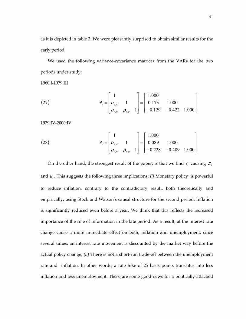
41

as it is depicted in table 2. We were pleasantly surprised to obtain similar results for the

early period.

We used the following variance-covariance matrices from the VARs for the two

periods under study:

1960:I-1979:III

( )27

−−=

=Ρ000.1422.0129.0

000.1173.0000.1

11

1

,,

,

urr

ue

ρρρ

π

π

1979:IV-2000:IV

( )28

−−=

=Ρ000.1489.0228.0

000.1089.0000.1

11

1

,,

,

urr

ue

ρρρ

π

π

On the other hand, the strongest result of the paper, is that we find tr causing tπ

and tu . This suggests the following three implications: (i) Monetary policy is powerful

to reduce inflation, contrary to the contradictory result, both theoretically and

empirically, using Stock and Watson’s causal structure for the second period. Inflation

is significantly reduced even before a year. We think that this reflects the increased

importance of the role of information in the late period. As a result, at the interest rate

change cause a more immediate effect on both, inflation and unemployment, since

several times, an interest rate movement is discounted by the market way before the

actual policy change; (ii) There is not a short-run trade-off between the unemployment

rate and inflation. In other words, a rate hike of 25 basis points translates into less

inflation and less unemployment. These are some good news for a politically-attached

42

policymaker. However, we have to take into account that it is a short-run effect indeed

and these actions increase variability, persistence negative effects on the employment

level; and (iii) a rate hike tends to come back to the “steady-state” in a more gradually.

These results takes more significance when we compare the three last impulse-

responses in figure 3 of both, the Stock and Watson’s and the ones based upon the

empirically-based DAG.

We want to emphasize that these results are based on an observed causal structure

only between inflation, unemployment rate, and the interest rate.

E. Conclusions

The strongest result of the paper, is that we find tr causing tπ and tu . This suggests

the following four implications: (i) Monetary policy is powerful to reduce inflation,

contrary to the contradictory result, both theoretically and empirically, using Stock and

Watson’s causal structure for the second period. Inflation is significantly reduced even

before a year. We think that this reflects the increased importance of the role of

information in the late period. As a result, at the interest rate change cause a more

immediate effect on both, inflation and unemployment, since several times, an interest

rate movement is discounted by the market way before the actual policy change; (ii)

There is not a short-run trade-off between the unemployment rate and inflation. In

other words, a rate hike of 25 basis points translates into less inflation and less

unemployment. These are some good news for a politically-attached policymaker.

43

However, we have to take into account that it is a short-run effect indeed and these

actions increase variability, persistence negative effects on the employment level; (iii)

The Fed has not followed a Taylor rule in any of the two periods under study; and (iv) a

rate hike tends to come back to the “steady-state” in a more gradually.

These results takes more significance when we compare the three last impulse-

responses in figure 3 of both, the Stock and Watson’s and the ones based upon the

empirically-based DAG.

We want to emphasize that these results are based on an observed causal structure

only between inflation, unemployment rate, and the interest rate.

44

CHAPTER III

PROBABILITY FORECASTING AND CENTRAL BANK ACCOUNTABILITY

If you twist my arm, you can make me give a single number as a guess about next year’s GNP. But you will have to twist hard. My scientific conscience would feel more comfortable giving you my subjective probability distribution for all the values of GNP. ― Paul A. Samuelson (1965), p. 278.

A. Introduction

For years the conduction of monetary policy and its executive board’s judgment and

motivation was a mystery to the general public. Central Bankers built reputations

making decisions in an environment of confidentiality. Arguments supporting a higher

degree of central bank transparency have recently persuaded monetary authorities to be

more open with respect to policymaking decisions, up to the point for some to make

their forecasts of the key variables public. Intensifying the public’s response to

monetary policy changes as transparency improves the public’s ability to predict policy

decisions reflected in the public’s actions, is among the potential gains of increased

transparency (Svensson, 1997; Woodford, 2003).

Transparency is related to accountability (Walsh, 2003). Given that central banks

have no absolute control over inflation and that monetary policy effects are observed

with time lags, making the central bank beliefs about the state of the economy available

ex ante through their forecasts, opens up new ways to assess whether the central bank’s

45

actions are consistent with their mandate27. Proper forecast evaluation methods are

among these.

In order to incorporate the inherent risks of macroeconomic policy, complete

probabilistic statements –namely density or probabilistic forecasts28 (Dawid, 1986)-,

rather than point-forecasts are preferred (Samuelson, 1965; Zarnowitz and Lambros,

1987; Chari, 1998; Svensson, 2003). What is even more compelling is that advances in

statistical methodology, as well as increases in computer power, have generated the

interest and use of probabilistic forecasts (Tay and Wallis, 2000) .

The Bank of England (BoE) is one of the few central banks that actually publish its

inflation forecasts29. The Monetary Policy Committee (MPC) of the BoE has been issuing

density forecasts of inflation –the so-called “Fan Charts”- on a quarterly basis in its

Inflation Report since August 1997. It has been issuing output growth forecasts since

November 1997. In addition, the BoE has published probabilistic forecasts of these two

“key” variables from a quarterly survey of undisclosed external forecasters, averaging

their responses for each range of the probability distribution.

The MPC has shown interest in the ex post evaluation of their ex ante density

forecasts30: “…the analysis of past forecast errors may help to shed light on deficiencies

27 This becomes less ambiguous in an explicit inflation targeting regime (Walsh, 2003)

28 The terms “density” and “probabilistic” are used interchangeably all across the paper.

29 Hatch (2001) provides an insightful introduction to the Bank of England’s modeling and forecasting. For detailed information on the construction of fan charts see Britton, Fisher and Whitley (1998).

30 The MPC asked Adrian Pagan (2003) to review their forecasts and assess their forecasting abilities in 2001.

46

in the models, as well as in the Committee’s thinking. For this reason the Bank conducts

regular analysis of its forecast errors.” (Bank of England, 2003).

Unfortunately, the Committee has only reported point-forecast evaluation

measures31, such as the average forecast errors of their mean projections. This suggests

two potential problems: First, point-forecast evaluation measures do not take into

account the forecaster’s assessment of the uncertainty associated with the forecast,

present in a complete probabilistic statement, such is the case of the “Fan Charts”.

Second, even though the MPC integrates external surveyed forecasts in their

Inflation Report, they do not report any forecast ability measurements of the

“others’” probability assessments. Thus there are no means to compare the

calculated metric and provide an objective appraisal of how “good” or “bad” is it.

We suggest that reported the probabilistic forecasts and ex-post evaluations on both

the MPC and an alternative “shadow” committee offers valuable information on

forecasting performance that is not available from reports on the MPC above. A

humorous epigraph, summarizing a conversation between person “A” and person

“B”, of Granger and Newbold (1986) illustrates well our suggestion: “A: How is

your wife? B: Compared to what?”

Probability calibration has been used to evaluate probability forecasts (Bunn, 1984;

Dawid, 1984; Kling and Bessler, 1989; Diebold, Hahn, and Tay, 1999; and the survey by

Tay and Wallis, 2000). Calibration is the ability to match the ex post relative frequency of

all events with the associated forecasted probability distribution (Dawid, 1984).

31 Surveyed by Wallis (1995).

47

Recently Wallis (2003, 2004) and Clements (2004) have performed calibration-based

analyses on the MPC one-year-ahead inflation density forecasts. They both agree that

the MPC overestimated the future uncertainty making the inflation probabilistic

forecasts “fan out” more rapidly. They also suggest the existence of biases by stressing

the MPC has placed too much probability in the upper ranges of the forecasted

distribution. While Wallis (2004) compares the MPC inflation forecasts with the ones

issued by the National Institute of Economic and Social Research 32 (NIESR), Wallis (2003)

and Clements (2004) do not offer comparisons with other forecasters.

A drawback of using calibration-based measures as the sole metric of “goodness” of

density forecasts is that calibration does not measure the resolution of the forecast. In

other words, by neglecting the ex post resolution of a density forecast, we are

overlooking the ability to sort the probabilities between the events that actually occur

from the ones that did not occur. As a result, a forecaster could be perfectly calibrated

and, at the same time, offer little to forecast users.

Although these issues in forecast evaluation have been present in the meteorology

literature for many decades (Brier, 1950; Sanders, 1963; Murphy, 1973; Yates, 1982,

1988), their discussion has not emerged in economics until recently. Zellner, Hong, and

Min (1991) use the Brier score, which captures both calibration and resolution to assess

turning forecasts from econometric models. More recently, Bessler and Ruffley (2004)

use the Brier score and its partition to assess probabilistic forecasts of stock market

returns. They offer an example of potential problems associated with using only

32 The National Institute of Economic and Social Research issues 1-quarter and 1-year-ahead probabilistic forecasts for inflation and output growth in the National Institute Economic Review since October 1996.

48

calibration when evaluating density forecasts. They provide means to overcome the

problem by exploiting two properties of the Brier score. First, it has been shown that the

Brier scoring rule encourages the forecaster to report their true beliefs. In this regard, an

affluent history unfolds on the use of quadratic scoring rules to motivate and evaluate

subjective probabilities, finding foundations on both theoretical (de Finetti, 1937, 1965

and 1974; Savage, 1971) and experimental grounds (Nelson and Bessler, 1989).

Furthermore, calibration does not necessarily encourage honesty (Winkler, 1986). If

agent (subject) knows he/she is being “judged” using calibrations, he/she can

misreport probabilities for the next period to compensate for already known

miscalibrations in earlier periods. By doing thishe/she might not be reporting what is

actually believed.

Second, the Brier score not only takes into account the calibration property, but also

relates to the ability of a forecaster (person or model) to sort events into groups: those

events which obtain versus those events which do not obtain, ex ante.

The Brier score can be decomposed in order to offer assessments on both calibration

and sorting (resolution) attributes of a probability forecast using its Yates’ partition

(Yates, 1982, 1988).

The purpose of this paper is to illustrate use of the Brier score and its Yates’

partition and suggest how such information may improve the degree of transparency of

the monetary authorities’ policy decisions, by increasing the ability to make the central

bank accountable for their actions. Such information, when used in conjunction with

similar information from a “shadow” committee can aid the central bank in improving

49

their probability forecasts and give private market participants clear signals on

monetary policy and its likely aggregate consequences. Our purpose falls well within

the ambit of study of the Bank’s own forecast assessments; only here we demonstrate

how one might perform such a study with a well defined proper scoring rule.

We propose the use the quadratic scoring rule to evaluate the central banks’

inflation (and output growth) density forecasts. These analyses are carried out under

the consideration that optimal density forecast evaluation is a necessary condition for

the forecast to work as an optimal accountability mechanism.

Recognizing the incentive-compatible feature of the Brier score, we considered (and

later ruled out) utilizing the Brier score in the context of a contract between the govt.

and the central bank in the spirit of Persson and Tabellini (1993, 1999, 2000), and Walsh

(1995a, 1998). Because of ambiguities –discussed in McCallum (1999) and Blinder

(1998)- that come into sight from applying this approach to central banking to the

letter33, this possibility is abandoned. Difficulties in determining whether it is the

principal (Parliament or Congress) or the agent (central bank), who has more incentive

to try to boost the real output in the short-run by creating “surprise inflation” is among

these ambiguities.

Hence, given the fact that there is no explicit reward-punishments agreement,

contingent to the realization of the states that were forecasted and the probabilities that

were issued to those events, in order to keep the incentive property of the Brier score,

33 In order to connect Walsh’s (1995a, 1998) and Persson and Tabellini’s (1993, 1999, 2000) contracting approach to our proposal, it had to be followed literally. Consequently it was not given any practical consideration. However, this should not be interpreted as discarding the importance of their contributions to improve the assessment of modern monetary policy issues.

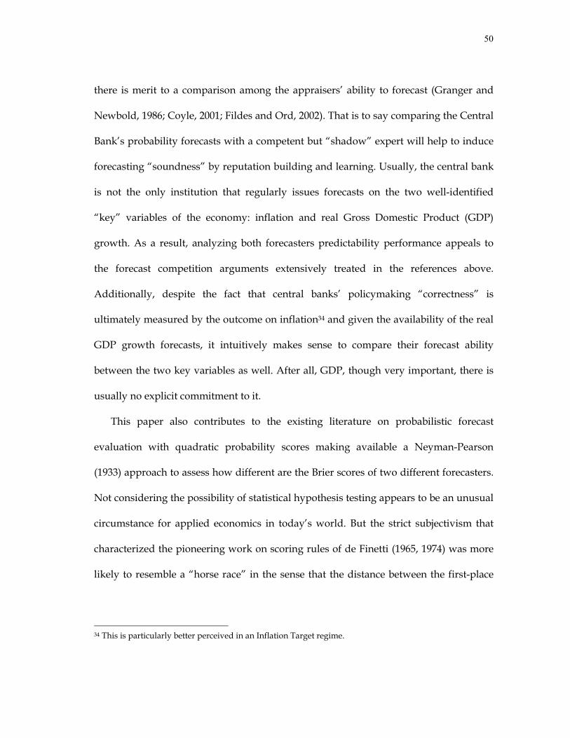
50

there is merit to a comparison among the appraisers’ ability to forecast (Granger and

Newbold, 1986; Coyle, 2001; Fildes and Ord, 2002). That is to say comparing the Central

Bank’s probability forecasts with a competent but “shadow” expert will help to induce

forecasting “soundness” by reputation building and learning. Usually, the central bank

is not the only institution that regularly issues forecasts on the two well-identified

“key” variables of the economy: inflation and real Gross Domestic Product (GDP)

growth. As a result, analyzing both forecasters predictability performance appeals to

the forecast competition arguments extensively treated in the references above.

Additionally, despite the fact that central banks’ policymaking “correctness” is

ultimately measured by the outcome on inflation34 and given the availability of the real

GDP growth forecasts, it intuitively makes sense to compare their forecast ability

between the two key variables as well. After all, GDP, though very important, there is

usually no explicit commitment to it.

This paper also contributes to the existing literature on probabilistic forecast

evaluation with quadratic probability scores making available a Neyman-Pearson

(1933) approach to assess how different are the Brier scores of two different forecasters.

Not considering the possibility of statistical hypothesis testing appears to be an unusual

circumstance for applied economics in today’s world. But the strict subjectivism that

characterized the pioneering work on scoring rules of de Finetti (1965, 1974) was more

likely to resemble a “horse race” in the sense that the distance between the first-place

34 This is particularly better perceived in an Inflation Target regime.

51

winner and the second-place arriving horse turns out to be completely irrelevant at the

moment of getting the prize.

This paper differs from Clements (2004), who also calculates the Brier Score of the

MPC forecasts, as we provide an idea of an incentive-compatible mechanism to

encourage honesty from the forecaster. Furthermore, we introduce the use of the Yates

decomposition as a technique to extract meaningful information about the forecaster’s

beliefs.

We find that the MPC is “upwardly” biased by placing larger probabilities to the

high state preventing the less conservative members of the Committee to gain any

approval for interest rate cuts. These results are consistent with Pagan (2003), Wallis

(2003, 2004) and Clements (2004).

The remainder of the paper is divided in four sections. The relationship between

transparency, accountability and proper forecast evaluation methods as reputation-

building mechanisms is described in the first section. Section C, provides an overview

of probabilistic forecasting concepts and shows the suggested density forecast

evaluation methodology with the theoretical rigorousness that characterizes the

process. The third part presents the empirical exercise of the techniques described on

Section C on the density forecasts of inflation and output growth of the MPC and the

external surveyed forecasters. Section E portrays the concluding discussions.

52

B. Transparency, Accountability, and Forecast Evaluation

1. Central Banks Tradition of Secrecy, Problems, and Proposed Solutions

It is well-known that “enigmatic” policymaking gives rise to highly uncertain

scenarios. Uncertainty about money and inflation weakens the role of the price system

as a mechanism of optimal resource allocation (Hayek, 1945). Furthermore, Friedman, et

al. (1949) argued that policy-induced uncertainty could lead both consumers and firms

to undertake actions they would not choose under certainty. He also claimed that the

source of the monetary authority’s “secrecy” was the central bankers’ dual goal of

maximizing their prestige and, at the same time, minimizing their accountability35.

The first proposed solution was to impose a fixed rule of monetary growth on the

central bank (Friedman, 1948, 1960). It has been argued that such rules are overly

restrictive, and that they do not provide the central bank with the sufficient

discretionary power to account for adverse shocks in the economy.

A “new” version of the “rules vs. discretion” debate -brought up by Kydland and

Prescott (1977), and Barro and Gordon (1983)- brought forth the utilization of dynamic

policy rules (Taylor, 1993, 1999 and McCallum, 1988, 1999 -among others-) to overcome

the concerns that could arise due to the celebrated “time inconsistency” problem, first

noticed in the monetary literature by Auernheimer (1974). Arguments against the

potential problems of “time inconsistency” (Mankiw, 1998 and Albanesi, Chari and

35 As quoted by Fischer (1990) and cited by Faust and Svensson (2000).

53

Christiano, 2001), in addition to the central bankers’ fear that even a dynamic policy

rule could still be stringent36, have made central banks hesitant to adopt these rules.

To overcome the dynamic inconsistency problem, Rogoff (1985) suggests hiring a

“conservative” central banker. Lamentably, finding out if a central banker is sufficiently

conservative or not, is not an easy task to perform as noted by Barro (1986) and recently

by Woodford (2003). In that case, another asymmetric information problem surfaces:

adverse selection at the time of deciding who to appoint as central banker. Yet, a moral

hazard problem remains.

An alternative scheme to face the “time inconsistency” problem has been the use of

contracts (Persson and Tabellini, 1993, 1999, 2000, and Walsh, 1995a, 1998). Here the

contract would design or specify a rewards-punishments scheme between the congress

and the central bank. On this issue, Garfinkel and Oh (1993) assert that legislation

punishing the monetary authority by reducing her salary or the central bank’s budget,

if she deviates from the target could be used to enforce the regime. Unfortunately, the

intrinsic complexity in modeling the government’s preferences causes serious

difficulties to build a totally applicable contract. Blinder (1998) criticizes this approach

by stating that the principal, by having a reelection period ahead, could have more

incentive to have an inflation bias than the agent, who is not supposed to be concern

about the political election process. Another point of disapproval is that salary is not a

36 Taylor (1993, 2000) acknowledges the remaining restrictions that these “activist” rules impose on central bank and suggests that, instead of making use these rules as systematic mechanisms to act to stabilize the economy, they could still be used as guidelines.

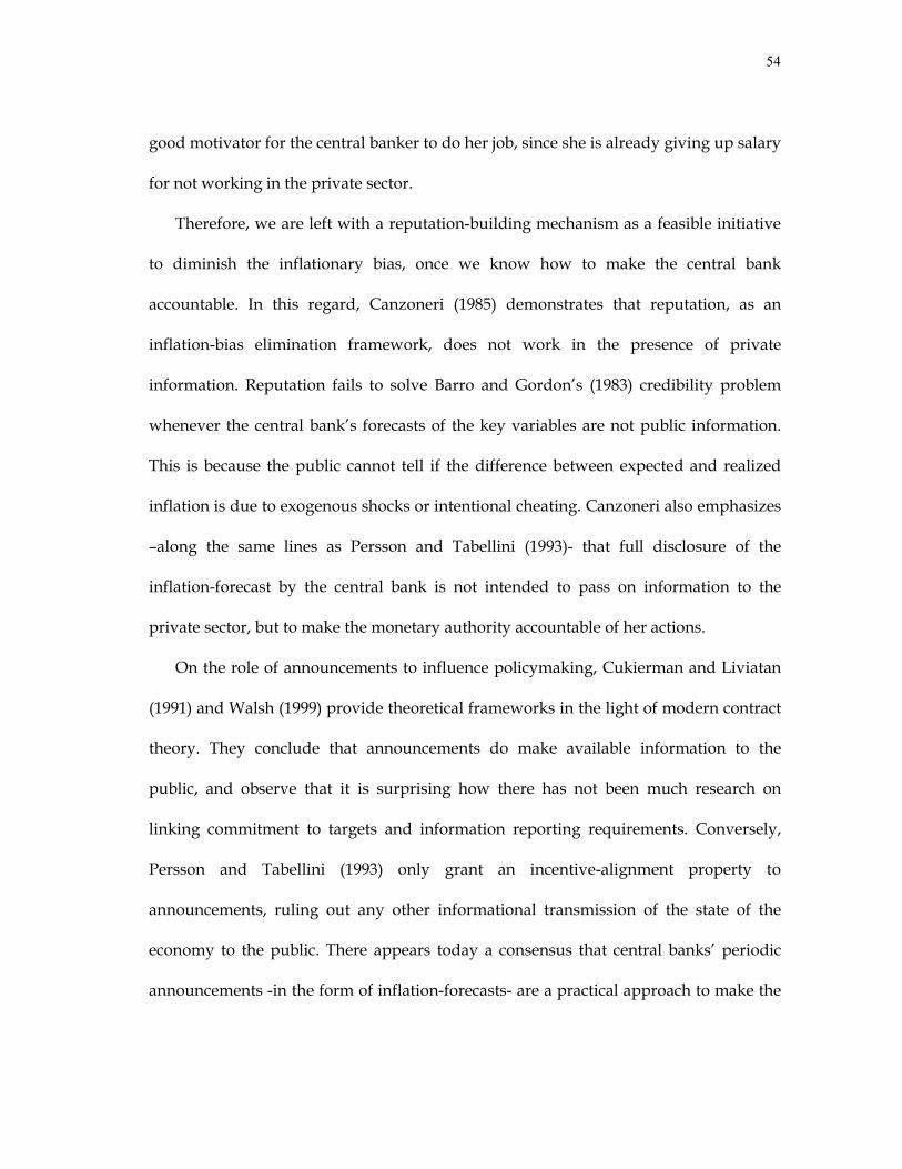
54

good motivator for the central banker to do her job, since she is already giving up salary

for not working in the private sector.

Therefore, we are left with a reputation-building mechanism as a feasible initiative

to diminish the inflationary bias, once we know how to make the central bank

accountable. In this regard, Canzoneri (1985) demonstrates that reputation, as an

inflation-bias elimination framework, does not work in the presence of private

information. Reputation fails to solve Barro and Gordon’s (1983) credibility problem

whenever the central bank’s forecasts of the key variables are not public information.

This is because the public cannot tell if the difference between expected and realized

inflation is due to exogenous shocks or intentional cheating. Canzoneri also emphasizes

–along the same lines as Persson and Tabellini (1993)- that full disclosure of the

inflation-forecast by the central bank is not intended to pass on information to the

private sector, but to make the monetary authority accountable of her actions.

On the role of announcements to influence policymaking, Cukierman and Liviatan

(1991) and Walsh (1999) provide theoretical frameworks in the light of modern contract

theory. They conclude that announcements do make available information to the

public, and observe that it is surprising how there has not been much research on

linking commitment to targets and information reporting requirements. Conversely,

Persson and Tabellini (1993) only grant an incentive-alignment property to

announcements, ruling out any other informational transmission of the state of the

economy to the public. There appears today a consensus that central banks’ periodic

announcements -in the form of inflation-forecasts- are a practical approach to make the

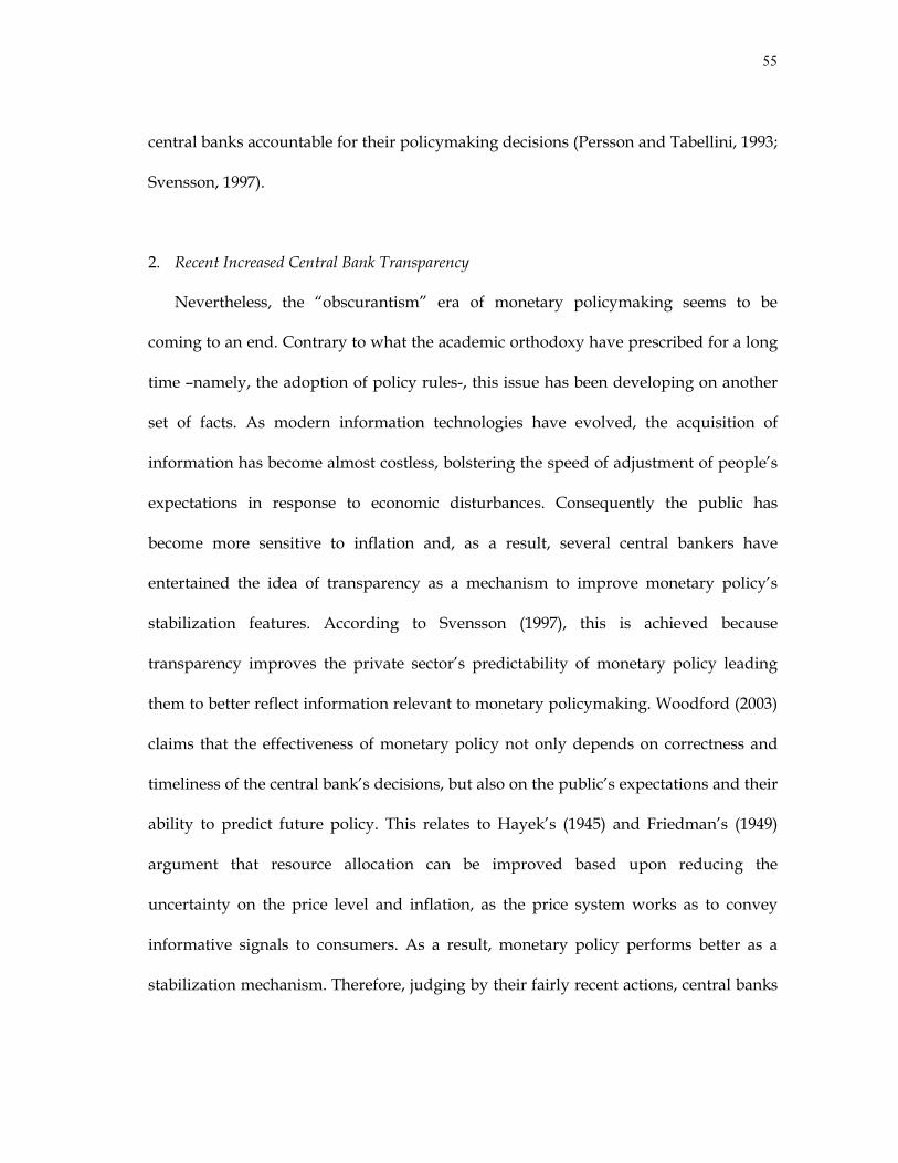
55

central banks accountable for their policymaking decisions (Persson and Tabellini, 1993;

Svensson, 1997).

2. Recent Increased Central Bank Transparency

Nevertheless, the “obscurantism” era of monetary policymaking seems to be

coming to an end. Contrary to what the academic orthodoxy have prescribed for a long

time –namely, the adoption of policy rules-, this issue has been developing on another

set of facts. As modern information technologies have evolved, the acquisition of

information has become almost costless, bolstering the speed of adjustment of people’s

expectations in response to economic disturbances. Consequently the public has

become more sensitive to inflation and, as a result, several central bankers have

entertained the idea of transparency as a mechanism to improve monetary policy’s

stabilization features. According to Svensson (1997), this is achieved because

transparency improves the private sector’s predictability of monetary policy leading

them to better reflect information relevant to monetary policymaking. Woodford (2003)

claims that the effectiveness of monetary policy not only depends on correctness and

timeliness of the central bank’s decisions, but also on the public’s expectations and their

ability to predict future policy. This relates to Hayek’s (1945) and Friedman’s (1949)

argument that resource allocation can be improved based upon reducing the

uncertainty on the price level and inflation, as the price system works as to convey

informative signals to consumers. As a result, monetary policy performs better as a

stabilization mechanism. Therefore, judging by their fairly recent actions, central banks

56

have been more in line with the role of actually providing the public with information

(Cukierman and Liviatan, 1991; Walsh, 1999).

In order to increase their transparency, several central banks have explicitly

committed to achieve a low and stable inflation. This has been achieved by Central Bank

Independence (CBI), and Inflation Targeting (IT). They also issue reports on inflation,

making their (and sometimes others’) forecasts public, and describing their expected

policy responses to face the forecasted future events.

CBI is described as the assignment of monetary policy to a central banker whose

decisions cannot be rejected ex post by the policymaker (Lippi, 1999). Herrendorf and

Neumann (1999) claim that a politically-detached independent central bank exhibits

less incentives to care about the government’s reelection chances reducing the

possibilities of using monetary policy to create surprise inflation37. But independence

could be associated with a greater degree of “conservativeness” in the Rogoff (1985)

sense. In other words, greater independence may imply less-active stabilization policies

and, therefore, higher output variance. This suggests that the gains of having an

independent central bank depend on the extent of the trade-off between the inflationary

bias and the variance of the policy targets. As a result, in addition to CBI, stability of

policy targets is desired to overcome the time-inconsistency problem (Lippi, 1999). CBI

and targeting regimes are not viewed as substitutes, but complements.

37 The monetary policy credibility issues have been criticized because, in reality, usually policymakers do not try to create unexpected inflation to surprise the private sector. But these criticisms miss the point that, in equilibrium, despite the monetary authority’s wish to reduce the inflation rate, it abstains from doing it because the disinflationary policy could turn into a recession, due to its lack of credibility.

57

IT is a mechanism that could be interpreted to be “in the middle” between full-

discretion and restriction. But still, even an inflation targeting regime, of a constrained

discretion regime country, could show an inflation bias if there is no incentive to

achieve the target. The ex-post measure that the IT regime provides as inflation and the

target could still not fully remove the inflation bias since there could be moral hazard.

The bank can always provide a somewhat “good” explanation of why she could not

achieve the target. Hence, additional to the inflation targeting regime, these points raise

the question of what can be done to eliminate the moral hazard that feeds the credibility

problem.

Yet central banks often do issue reports on inflation, making their (and sometimes

others’) forecasts public, and describing their expected policy responses to face the

forecasted future events. Justification for this central banks behavior is along the same

lines as Hayek (1945), Friedman, et al. (1949), and Svensson (1997), rather than on the

Canzoneri (1985) sense.

With respect to the publication of inflation forecasts, although this is a plausible on

possible means to increase transparency, this does not necessarily ensure transparency.

Walsh (2003) defines the degree of transparency as the ability to monitor the central

bank. Under imperfect information, it is optimal for the monetary authority to place less

weight on achieving the inflation target. To solve this problem he suggests to create a

high-powered incentive structure, based on optimal performance measures (Baker,

1992), to motivate the central banks not only publish their inflation forecasts but, by

doing this, attain transparency as well. In other words, with perfect monitoring, the

58

central bank’s only goal is to care about achieving the desired level of inflation (or

inflation target).

Summarizing the above, on one hand, greater transparency is prone to trim down

uncertainty and help monetary policy performance. On the other hand, greater

accountability is likely to improve incentives to be really transparent and get rid of the

inflationary bias. However, for transparency to work, besides making the central bank’s

forecasts public, we need an incentive structure that allows perfect monitoring.

3. Forecasting as a Reputation-Building Mechanism

For the publication of the forecast to increase transparency a la Walsh (2003), a way

to monitor the central bank must be found. For the forecast to work as a reputation-

building mechanism in the Canzoneri (1985) sense, it should neither be private

information nor a disturbance element. In decision theory jargon, the forecast needs to

satisfy two conditions: (i) have full disclosure of the forecast and the forecast generation

methods, and (ii) the forecast has to be a “good” forecast (Winkler, 1986). By this, we

mean that, it must reflect the banks’ true beliefs. When outcomes are uncertain,

planning must be based on forecasts. Naturally, the planner wishes to ensure that these

forecasts are prepare honestly and with an appropriate degree of care (Winkler, 1986;

Osband, 1989).

The forecast must be an accurate forecast as well. So not only should the central

banker provide their true beliefs about their future expectations on inflation (and, if

there is the case, on GDP as well), but also exert their best effort to provide a “good”

59

forecast. Walsh (2003) proposes the use of optimal measures of (forecast) performance

for accountability to be transformed into transparency. Therefore we need an optimal

way to evaluate the central banks forecasting performance on the key variable -namely

inflation- that honors both honesty and accuracy. The Brier Score and its partition (by

Yates, 1982, 1988) actually promotes both.

4. Density Forecasts in Monetary Policy

If we want to take into account the uncertainties that surround the forecast, it is

recommended to be in probabilistic form (Samuelson, 1965). In the spirit of Robert E.

Lucas’ contributions to modern macroeconomics, Chari (1998) wrote: “Economists

today routinely analyze systems in which agents operate in complex probabilistic

environments to understand (their) interactions…”. Thus, an inflation-forecast,

provided as a complete probabilistic statement is desired. Furthermore, Svensson (2003)

points out that in an inflation-forecast targeting setting, a point-forecast only works

under the following three assumptions: (i) quadratic loss function, (ii) linear

transmission mechanism, and (iii) additive uncertainty. The first assumption is

reasonable and widely used (Kydland-Prescott, 1977, and Barro and Gordon, 1983), and

it is supported by more recent research led by Blinder (1998), Svensson (2001), and

others.

The second assumption -linear transmission mechanism- is quite strong, since it

means that the future target variables depend on the current state of the economy and

the instrument, in a linear fashion. This is not likely to happen (Svensson, 2003).

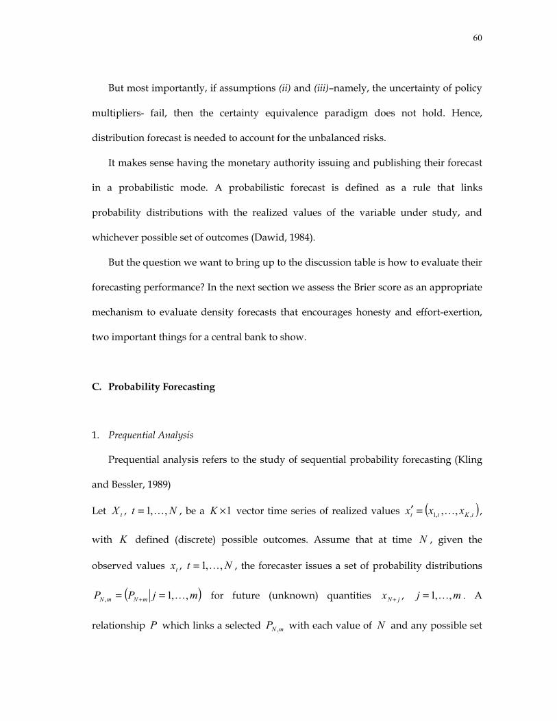
60

But most importantly, if assumptions (ii) and (iii)–namely, the uncertainty of policy

multipliers- fail, then the certainty equivalence paradigm does not hold. Hence,

distribution forecast is needed to account for the unbalanced risks.

It makes sense having the monetary authority issuing and publishing their forecast

in a probabilistic mode. A probabilistic forecast is defined as a rule that links

probability distributions with the realized values of the variable under study, and

whichever possible set of outcomes (Dawid, 1984).

But the question we want to bring up to the discussion table is how to evaluate their

forecasting performance? In the next section we assess the Brier score as an appropriate

mechanism to evaluate density forecasts that encourages honesty and effort-exertion,

two important things for a central bank to show.

C. Probability Forecasting

1. Prequential Analysis

Prequential analysis refers to the study of sequential probability forecasting (Kling

and Bessler, 1989)

Let tX , Nt ,,1…= , be a 1×K vector time series of realized values ( )tKtt xxx ,,1 ,,…=′ ,

with K defined (discrete) possible outcomes. Assume that at time N , given the

observed values tx , Nt ,,1…= , the forecaster issues a set of probability distributions

( )mjPP mNmN ,,1, …== + for future (unknown) quantities jNx + , mj ,,1…= . A

relationship P which links a selected mNP , with each value of N and any possible set

61

of outcomes tx , mNNt ++= ,,1… , is defined as a “prequential forecasting system”

(PFS) (Dawid, 1984). Although we could think of models, this could also apply to

subjective probability judgments as well (Kling and Bessler, 1989).

2. Probability Forecast Evaluation

According to Winkler (1996) to judge whether a probability forecast is good or bad

there are three aspects: coherence, expertise and calibration. In the current literature we

still find that this is what has been used to evaluate forecasts is the concept of

calibration. In other words, the ability to match the ex post relative frequency of all

events with the associated ex ante forecasted probability distribution.

3. Empirical Assessment of Calibration

If the quantities mtx + for each Kk ,,1 …= are random variables with distribution

functions mtF + for every Kk ,,1 …= , then the random fractiles ( )mtkmtkmtk xFQ +++ = ,,,

have a distribution function of the form ( ) mtkmtk qqG ++ = ,, . In the case of continuous

random variables, the random fractiles are independently and uniformly distributed

[ ]1,0U . In both the continuous and discrete cases the evaluation of a PFS can be

achieved if we test that the observed sequence mtkx +, was drawn from a probability

distribution with cumulative distribution ( ) mtkmtk qqG ++ = ,, . The forecaster is considered

to be well-calibrated if this hypothesis cannot be rejected. In order to obtain the

estimated distribution function ( )mtkqG +,ˆ for mtkQ +, Bunn (1984) suggests a three-step

62

procedure. First he recommend to take the observed sequence ( )mtkmtkmtk xFq +++ = ,,, ,

Nt ,,1…= and order them in an ascending sort.

Step two consists in calculating the following empirical cumulative distribution

function also referred as “calibration function” (Bunn, 1984):

( )29 ( )[ ] ( ) NjNjjqG jk ,,1,ˆ, …==

The graph of a well-calibrated PFS should look similar to a 45-degree line.

Third, test the observed fractiles iq ’s from the sequence of N probability forecasts

mtP , . Under the null hypothesis of well-calibration, any subinterval of length [ ]1,0∈L

will have NL ∗ observed fractiles. A chi-squared goodness-of-fit test could be utilized

if there are J non-overlapping subintervals that exhaust the unit interval.

( )30 ( )[ ] 211

22 ~ −=∑ −= JJ

j jjj NLNL χκχ

where jκ is the number of observed fractiles in the interval j and jL is the length of

interval j . The test statistic is distributed as a chi-squared with 1−J degrees of

freedom, if independence of the underlying distributions is not required (Dawid, 1984).

According to Winkler (1996) to judge if it is good or bad there are three aspects:

coherence, expertise and calibration. In the current literature we still find that this is

what has been used to evaluate forecasts is the concept of calibration. In other words,

the ability to match the ex post relative frequency of all events with the associated ex ante

forecasted probability distribution.

Bessler and Ruffley (2004) presented the major potential problem of using only

calibration-based forecast evaluation methods: Neglecting the ability to sort the

63

probabilities between the events that actually occur from the ones that did not occur.

Consequently, a forecaster could be perfectly calibrated but, at the same time, way too

wrong.

4. Scoring Rules

Let kr be the forecaster’s believed (discrete) probability judgments38 for every

possible event Kk ,,1 …= , where K is the number of possible outcomes, and kp the

reported probability of event k occurring. A scoring rule S is a one-to-one real-valued

function that assigns a score kS to a reported probability kp if event k did not occur,

and a score kj SS ≠ , kj ≠ to a stated probability jp if event k did occur39, regardless

of the appraiser’s true beliefs, i.e. kp need not be equal to kr , for all k . We

acknowledge that we are providing a somewhat restricted definition of scoring rules,

but we consider that its simplicity serves for our purpose without significantly

sacrificing rigorousness. For a more general definition of scoring rules, please see

Winkler (1986) and Selten (1998), pg. 45-46. jS can either be larger or smaller than kS ,

depending on the nature of the scoring rule. e.g. in the case of a linear scoring rule,

kj SS > , in the case of the quadratic rule would be the opposite.

38 Although we are only considering discrete probability distributions, this can be easily extended to the continuous distribution case as well (Winkler, 1986).

39 jS can either be larger or smaller than kS , depending on the nature of the scoring rule. e.g. in the case of

a linear scoring rule, kj SS > , in the case of the quadratic rule would be the opposite.

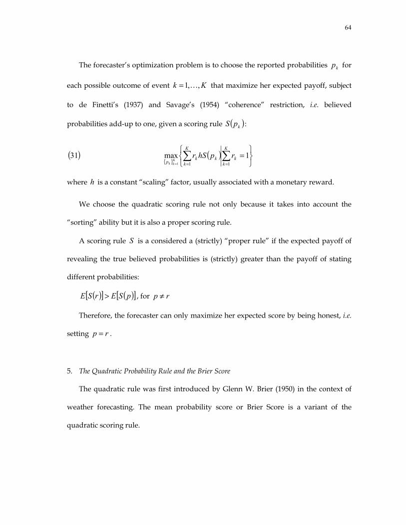
64

The forecaster’s optimization problem is to choose the reported probabilities kp for

each possible outcome of event Kk ,,1…= that maximize her expected payoff, subject

to de Finetti’s (1937) and Savage’s (1954) “coherence” restriction, i.e. believed

probabilities add-up to one, given a scoring rule ( )kpS :

( )31 { }

( )

=∑∑===

K

kk

K

kkk

prphSr

Kkk 11

1max1

where h is a constant “scaling” factor, usually associated with a monetary reward.

We choose the quadratic scoring rule not only because it takes into account the

“sorting” ability but it is also a proper scoring rule.

A scoring rule S is a considered a (strictly) “proper rule” if the expected payoff of

revealing the true believed probabilities is (strictly) greater than the payoff of stating

different probabilities:

( )[ ] ( )[ ]pSErSE > , for rp ≠

Therefore, the forecaster can only maximize her expected score by being honest, i.e.

setting rp = .

5. The Quadratic Probability Rule and the Brier Score

The quadratic rule was first introduced by Glenn W. Brier (1950) in the context of

weather forecasting. The mean probability score or Brier Score is a variant of the

quadratic scoring rule.

65

The Brier score belongs to a set of rules called “proper” rules or, in modern contract

theory terminology, of incentive-compatible forecasting scores. This means that these

rules encourage honesty (Winkler, 1996; Osband, 1989). There is a rich history on the

use of quadratic scoring rules to motivate and evaluate subjective probabilities, finding

strong foundations on both theoretical (de Finetti, 1937, 1965 and 1974; Savage, 1971)

and experimental (Nelson and Bessler, 1989) fields.

Let the probabilistic forecast of an event k occurrence be denoted by p , d be a

vector defined as the outcome index for event k as follows:

=01

d

The Quadratic Probability Score ( PS ) for a single forecast is:

( )32 ( ) ( ) 10,, 2 ≤≤−= PSdpdpPS

PS ranges between 0 and 1. A score of zero means that the forecaster did a “great job”

and predicted the events perfectly. We can see that PS is a loss function, rather than a

positive score. A forecaster who actually did extremely “bad” gets a 1.

PROPOSITION 1: The Quadratic Probability Score ( PS ) is a truth-probability-revelation

mechanism, i.e. PS is a “proper” scoring rule.

PROOF: To show that PS is a “proper” scoring rule, then we have to show that

rp = is the argument that maximize the forecaster’s optimization problem ( )31 . For

simplicity we set the scaling factor h to 21 . Since PS is a single-forecast (two-

outcome) rule, 2=k . Thus, imposing the “coherence” constraint (all the probabilities

If event k occurs

If event k does not occur

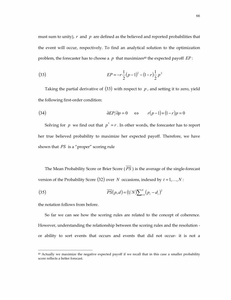
66

must sum to unity), r and p are defined as the believed and reported probabilities that

the event will occur, respectively. To find an analytical solution to the optimization

problem, the forecaster has to choose a p that maximizes40 the expected payoff EP :

( )33 ( ) ( ) 22

2111

21 prprEP −−−−=

Taking the partial derivative of ( )33 with respect to p , and setting it to zero, yield

the following first-order condition:

( )34 0=∂∂ pEP ⇔ ( ) ( ) 011 =−+− prpr

Solving for p we find out that rp =* . In other words, the forecaster has to report

her true believed probability to maximize her expected payoff. Therefore, we have

shown that PS is a “proper” scoring rule

The Mean Probability Score or Brier Score ( PS ) is the average of the single-forecast

version of the Probability Score ( )32 over N occasions, indexed by Nt ,,1…= :

( )35 ( ) ( ) ( )∑ =−= N

t tt dpNdpPS1

21,

the notation follows from before.

So far we can see how the scoring rules are related to the concept of coherence.

However, understanding the relationship between the scoring rules and the resolution -

or ability to sort events that occurs and events that did not occur- it is not a

40 Actually we maximize the negative expected payoff if we recall that in this case a smaller probability score reflects a better forecast.

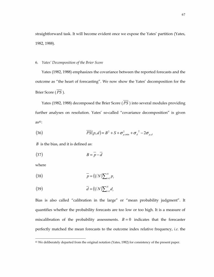
67

straightforward task. It will become evident once we expose the Yates’ partition (Yates,

1982, 1988).

6. Yates’ Decomposition of the Brier Score

Yates (1982, 1988) emphasizes the covariance between the reported forecasts and the

outcome as “the heart of forecasting”. We now show the Yates’ decomposition for the

Brier Score ( PS ).

Yates (1982, 1988) decomposed the Brier Score ( PS ) into several modules providing

further analyses on resolution. Yates’ so-called “covariance decomposition” is given

as41:

( )36 ( ) dpdpSBdpPS ,22

min,2 2, σσσ −+++=

B is the bias, and it is defined as:

( )37 dpB −=

where

( )38 ( )∑ == N

t tpNp1

1

( )39 ( )∑ == N

t tdNd1

1

Bias is also called “calibration in the large” or “mean probability judgment”. It

quantifies whether the probability forecasts are too low or too high. It is a measure of

miscalibration of the probability assessments. 0=B indicates that the forecaster

perfectly matched the mean forecasts to the outcome index relative frequency, i.e. the

41 We deliberately departed from the original notation (Yates, 1982) for consistency of the present paper.

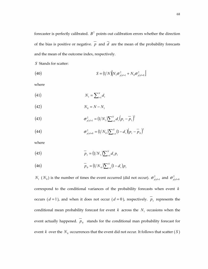
68

forecaster is perfectly calibrated. 2B points out calibration errors whether the direction

of the bias is positive or negative. p and d are the mean of the probability forecasts

and the mean of the outcome index, respectively.

S Stands for scatter:

( )40 ( )[ ]200

2111 == += dpdp NNNS σσ

where

( )41 ∑ == N

t tdN11

( )42 10 NNN −=

( )43 ( ) ( )∑ == −= N

t ttdp ppdN1

2

112

1 1σ

( )44 ( ) ( )( )∑ == −−= N

t ttdp ppdN1

2

002

0 11σ

where

( )45 ( )∑ == N

t tt pdNp111 1

( )46 ( ) ( )∑ =−= N

t tt pdNp100 11

1N ( 0N ) is the number of times the event occurred (did not occur). 21=dpσ and 2

0=dpσ

correspond to the conditional variances of the probability forecasts when event k

occurs ( 1=d ), and when it does not occur ( 0=d ), respectively. 1p represents the

conditional mean probability forecast for event k across the 1N occasions when the

event actually happened. 0p stands for the conditional man probability forecast for

event k over the 0N occurrences that the event did not occur. It follows that scatter ( S )

69

is the weighted average of 21=dpσ and 2

0=dpσ , and it can be interpreted as an index of

general “excess” variability (or noise) contained in the forecaster’s probability

statements.

2min,pσ is the minimum variance of the forecast, and it is defined as:

( )47 Spp −= 22min, σσ

where

( )48 ( ) ( )∑ =−= N

t tp ppN1

22 1σ

S is the scatter, defined in equation ( )40 , 2pσ is the total variance of the issued density

forecast, and p is defined in ( )38 . Notice that 2min,pσ equals the overall forecast

variance whenever there is no scatter ( 0=S ) about the conditional means of 1p and

0p .

2dσ is the variance of the outcome index d and defined as:

( )49 ( )ddd −= 12σ

where d is defined in equation ( )39 .

dp,σ is the covariance between the forecasted probabilities and the outcome index,

given by:

( )50 2, ddp θσσ =

where θ is the slope, and it is given by the following expression:

70

( )51 01 pp −=θ

[ ]1,0∈θ The maximum value of θ is 1 and it occurs whenever the forecaster reports

1=p when the event occurred and 0=p when the event did not occur.

Given that 2dσ is completely exogenous to the forecaster’s judgments, the appraiser

has to minimize S and 2min,pσ and maximize dp,σ in order to minimize the PS .

dp,σ , follows. dp,σ measures the responsiveness of the forecaster to information

related to event k ’s occurrence, and S indexes the forecaster’s responsiveness to

information not related to event k ’s occurrence.

Having presented the technical aspects of the Brier score and its Yates’ partition, we

are able to show formally that using calibration-based forecast performance measures

only is not the best way to evaluate density forecasts.

PROPOSITION 2: Suppose that a forecaster obtains a perfect Brier score. Then the

forecaster is also perfectly calibrated, but not the converse.

PROOF: Assume that 02 ≠B , i.e. the forecaster is somewhat miscalibrated. By

multiplying and dividing the term dp,σ in equation ( )36 by 22pd σσ , the

correlation between p and d , denoted by dp,ρ , becomes explicit:

( )52 22,

222 2 dpdpdpBPS σσρσσ −++=

Suppose that forecaster has perfect foresight. This implies that the forecaster has to

match the total variance of the outcome index and the total variance of the issued

forecast, i.e. 22dp σσ = .

71

( )53 2,

22 22 pdppBPS σρσ −+=

A perfect forecaster achieves a Brier score of zero. By definition, this implies that the

correlation coefficient between the probability forecast and the outcome index equals

the unity. It follows that 02 =B and contradicts the initial statement of this proof.

We have demonstrated the first part of the proposition. We now turn to the second

part. Since we just need to find an exception to complete this proof, we are going to set

the conditions under which a perfectly calibrated forecaster does not achieve the

minimum (best) Brier score. Assume the forecaster is perfectly calibrated, i.e. 02 =B .

Suppose the forecaster assigned a probability of zero to every outcome that occurred. In

addition, assume that without incurring in any miscalibration, resulting in a correlation

between the forecasted probabilities and the outcome index strictly less than 21 .

Furthermore, for simplicity, let’s assume that 022 ≠= dp σσ . Under these assumptions,

equation ( )52 can be expressed as:

( )54 ( )dppPS ,2 212 ρσ −=

It follows that the Brier score cannot be zero.

Proposition 2 allowed us to see that calibration is a necessary but not sufficient

condition to achieve the Brier score maximum attainable value.

Table 3 portrays a simple numerical example to illustrate proposition 2. It can be

observed that the forecasted probabilities match the relative frequency of the outcome

index on realized inflation, i.e. the forecaster predicted that inflation would fall once

within every range, and that is what happened. The problem here is that the forecaster

72

did not have the ability to discriminate between the events that occur and the ones that

did not occur. This ability was referred as the “resolution” of the forecast. The Brier

score takes into account both calibration and resolution.

7. The Multiple-Event Brier Score

The Brier mean probability score can also be expressed for a more than two-event

case, i.e. 2>K . In order to show this feature, let’s introduce the probability score ( PS )

for the multiple-event case (Murphy, 1973), then we will show that it is a “proper”

scoring rule as well, followed by the formulation for the Brier mean probability score

for K events and its Yates’ decomposition.

Let kd be the outcome index for each event Kk ,,1…= and kp represent the

probability forecasts for each event Kk ,,1…= . The multiple-event probability score is:

( )55 ( ) ( )∑ =−= K

k kk dpdpPSM1

2,

where 20 ≤≤ PSM . In this case, kd can be seen as the observed relative frequency

distribution over the outcomes Kk ,,1…= .

Although we consider that the proof of proposition 1 is intuitive, it cannot be

generalized for a multiple event case.

PROPOSITION 3. The Multiple-Event Probability Score ( PSM ) is a “proper scoring

rule”

PROOF. To demonstrate that PSM is a “proper” scoring rule, the forecaster should

choose to report her believed probability judgments for all the possible outcomes. In

73

other words, that kk rp = for all Kk ,,1…= are the arguments that maximize the

forecaster’s optimization problem ( )31 .

If outcome j occurs, 1=jd , and 0=kd , jk ≠∀ , elaborating the summation on

the PSM , equation ( )53 , and gathering terms, we are left with:

( )56 ( ) ∑ =+−= K

k kjj ppdpPSM1

221,

To find an analytical solution to the optimization problem, the forecaster has to

choose the set of kp ’s that maximize the expected payoff (For simplicity and without

loss of generality we set the scaling factor h to 1). The forecasters’ expected payoff is

the following:

( )57 ( )[ ] ( )∑∑ ==+−= K

k kjK

j jj pprdpPSME1

21

21,

Remember that the Brier score is a loss function, therefore, in this case we minimize

the forecaster’s expected payoff, [ ]jPSME , thus we maximize the negative of

[ ]jPSME . Setting the partial derivatives of the expected payoff (with respect to kp ,

Kk ,,1…=∀ ) to zero, yield the following first-order conditions:

( )58 Kkrpr K

k kkk ,,1,0221

…=∀=− ∑ =

By coherence, i.e. 11

=∑ =

K

k kr , it follows that kk rp =∗ , Kk ,,1…=∀ .

Therefore, we are only left with the task of showing that choosing kk rp =∗ for

every event k actually maximizes the forecaster’s (negative) payoff.

74

To ensure that a maximum is achieved, the second-order sufficient condition for a

minimum is that the matrix of second derivatives (Hessian) must be negative definite42.

A symmetric matrix is negative definite if and only if its K leading principal minors

have the same sign as ( )k1− .

In this case, it is easy to show that the Hessian matrix is negative definite because

the second crossed partial derivatives are zero and, restricting for “coherence”

( 11

=∑ =

K

k kr ), the diagonal elements are all equal to 2− , i.e.

[ ] 021

22 <−=∂∂ ∑ =

K

k kkj rpPSME , Kk ,,1…=∀ .

( )59 …

�

��

�

�

0,0,0,

20000

020002

321 <><

−

−−

= HHHH

We have shown that:

( )60 { }

( )[ ]{ }dpPSMErpKkkp

kk ,maxarg,1

−≡==

∗

In other words, the forecaster has to report her true believed probabilities to

maximize her expected payoff for each outcome Kk ,,1…= . Therefore, we have shown

that the PSM is a “proper” scoring rule

The multiple-outcome mean probability score or multiple-event Brier score is:

( )61 k

K

kPSPSM ∑ =

=1

where PS is defined in ( )35 .

42 Simon and Blume (1994), pg. 382.

75

The covariance decomposition due to Yates (1982, 1988) is:

( )62 ( ) ( ) ( )∑∑∑∑∑=====

−+++=K

kkdp

K

kkd

K

kkp

K

kk

K

kk SBPSM

1,

1

2

1

2min,

11

2 2 σσσ

where each component has a similar interpretation as the single-event case ( )36 .

8. Which Score Shall We Calculate? The Probability Score or the Mean Probability Score?

To encourage honesty and effort, the multiple-event probability score ( PSM ), and

not the mean probability score ( PSM ), should be calculated upon the last reported

forecast, for every publication of BoE’s Inflation Report. For example, when deFinetti

(1965), and Nelson and Bessler (1989) worked experimentally, they had to pay based

upon the last reported forecast, not the overall performance metric. This is because as

N goes to infinity, the marginal time-value of PSM tends to zero. Consequently, the

evaluated entity’s (in this case BoE) effort is not encouraged. But it is very important to

evaluate the overall performance as well. Not only because a “big picture” indicator of

performance is desired but, on the other hand, by calculating the PSM , you extract

information –by utilizing the Yates’ partition- to characterize their forecasting

performance with more detail. Therefore, the two indicators, PSM and PSM are

complements, not substitutes.

9. Hypothesis Testing for the Brier Score

We have assessed the importance of comparing the central bank’s forecasts with

other forecasters, in the first place. On the other hand, we have said that it is important

76

to compare to different variables, one in which the forecaster has special value

(inflation) and other that is not that important (GDP growth). Now, we ask the

question, how different are the multi-event case of the Brier Score ( PSM )?

As we call attention to this issue earlier in the paper, although the original purpose

of using scoring rules by de Finetti (1965, 1974) was more likely to resemble a “horse

race” in the sense that the distance between the first-place winner and the second-place

arriving horse turns out to be completely irrelevant at the moment of getting the prize,

not considering the possibility of statistical hypothesis testing appears to be an unusual

circumstance for applied economics.

In other words, we try to provide answers to the question on how different are the

probability judgment performances of both the central bank and the “other” forecasters.

We consider both positive and negative differences, in other words a two-tailed test.

When comparing two means of dependent or “paired” data, Freund (1992) suggest the

use of the following parametric test for the differences of the multiple-event probability

scores at each point in time Nt ,,1…=

The null hypothesis that the multiple-event Brier mean probability scores issued by

different forecasters is:

( )63 0: =− OFMPCO PSMPSMH

We propose the use of the CB -statistic:

( )64 ( )[ ] ( )NsPSMNCB ∆∆−∆= /1 µ

77

where

( )65 ( )∑ =−=∆ N

t tOFtMPC PSMPSMPSM1 ,,

( )66 ( )∑ =−=∆ N

t tOFtMPC PSMPSMPSM1

2,,

2

( )67 ( )[ ] ( )( )[ ]22 111 PSMNPSMNs ∆−∆−=∆

In the case of small samples (like the one we have got), using the “rule of thumb”

30<N , Freund (1992) suggests that we should contrast the CB -statistic with a 1,2 −ntα .

Whenever we have a large sample, Freund (1992) suggests contrasting the same

statistic with a z distribution instead of a student t distribution.

The CB -test proposed here assumes a common thing in economics, normality of the

differences of the multiple-event probability scores ( PSM∆ ). If we are concerned that

this could be a strong assumption, normality tests could be performed on the PSM∆

series in order to validate the statistical inference performed by the CB -test. According

to a recent survey by Dufour, et al. (1998), the most widely used normality tests in the

econometrics literature are the Jarque-Bera (1980, 1987), Kolmogorov-Smirnov

(Kolmogorov, 1933; Smirnov, 1939), Shapiro-Wilk (1965), Anderson-Darling (1954),

Cramér-von Mises (1928), and the D’Agostino (1971). Given the well-known trade offs

between using one test or the other; we leave this choice to the forecaster.

An alternative approach to the CB -test, if you happen to find out that your

multiple-event probability score differences are not distributed normally, is to use

certain non-parametric tests, such as the Wilcoxen Signed-Rank test. This

78

nonparametric approach utilizes the magnitude of the rank and the sign of the

differences between the pairs of measurements43.

D. Bank of England Fan Charts Evaluation

1. Bank of England Inflation Report

The Monetary Policy Committee (MPC) took responsibility of publishing an Inflation

Report on a quarterly basis when the BoE was given the operational independence in

1997. The MPC has been publishing their inflation forecast presenting the so-called

“Fan-Charts” or “Rivers of Blood” (term coined by Coyle, 2001) since August 1997.

These forecasts are conditional to the assumption that the interest rates remain constant

at the level the MPC decided. The committee reports their projections for one-quarter

up to eight-quarters ahead. The MPC meets every first Wednesday and Thursday

following the first Monday of each month, and they issue their forecasts at the

February, May, August and November meetings.

Figure 4 depicts the historical retail price index excluding mortgage interest

payments (RPIX) inflation since and, as the graph “fans out” it portrays the probability

of various outcomes for the future inflation. These projections are based on constant

nominal interest rates at 4 percent (Bank of England’s Inflation Report, May 2003). The

BoE’s inflation target was based on the RPIX until December 2003, when the MPC

changed the target to inflation based on the CPI.

43 For a useful illustration of this test, please refer to Ott and Longnecker (2001), pp. 308-312.

79

We assess the MPC and the “others” density forecast evaluations for the February,

1998–May, 2001 forecasts of inflation and GDP growth rate for the first quarter of 2000

to the second quarter of 2003. Although the MPC started reporting their inflation

forecasts in a density form in August 1997, they did not report the GDP until Nov. 1997.

Moreover, the real GDP growth density forecast for the Nov. ’97 is only reported as a

Fan Chart and not an explicit table.

The Brier score is said to work only for unconditional forecast evaluations

(Clements and Smith, 2002). Clements (2004) and Wallis (2003, 2004) discuss that the

one-year-ahead forecasts can be treated as unconditional forecasts since interest rates

do not have such an impact on inflation in the short-run. However, due to the lack of

consistent one-year-ahead forecasts issued by the external surveyed forecasters –

published in the Inflation Report-, we focus our analysis on the two-year-ahead forecasts.

Clements and Smith (2002) conclude that evaluating conditional forecasts with

unconditionally-related forecast evaluation techniques is not a major drawback if the

data set is sufficiently small (that is our case). Furthermore, exploring better methods

becomes worthwhile as the focus of the analysis lies on larger data sets. On the other

hand, evaluating the two-year density forecasts is important since longer term

forecasting horizons are usually related to the establishment of central bank credibility.

The BoE has issued Fan Charts conditional on a constant interest rate. Since

February 1997, the MPC has published fan charts conditional to the market expectations

of the interest rate. They perform this analysis by extracting information from the

80

implied volatilities from the market for options on government bonds with different

maturities (see Bahra, 1997).

2. Probability Scores, Brier Scores and Yates’ Partitions of the Density Forecasts of the UK

Here we calculate the multiple-event probability scores ( PSM ) for each quarter’s

forecast of inflation and the output growth rate, for both the MPC and the BoE’s

surveyed forecasters.

Figures 5 and 6 illustrate the MPC’s and the “other” forecasters’ PSMs obtained for

their assessments on the forecasts of inflation and output growth. On first sight, the

upward trend in both graphs caught our attention44. A hypothesis emerged from the

“learning-by-doing” theories could make us think experience in forecasting is grained

as time goes and better scores can be achieved. We do not find support for these ideas.

Unfortunately, the analysis is performed on very few observations. On the other hand,

they both run into the same trend, so it is not clear that this is an issue.

An oddity that becomes apparent is the “spike” in the forecast for the second

quarter of 2002, published on May, 2000. While this appears in both the MPC and the

surveyed forecasters’ PSMs, it is clearly a more dramatic one for the “other” forecasters.

The “overresponsiveness” shown by the surveyed forecasters might have been

explained because the MPC changes their surveyed sources from time to time without

notice. In the search for an extraordinary event –directly related to the MPC’s decisions-

during the dates the forecast was issued, we found an unprecedented “scandal”

44 Recall that the multiple-event probability score ranges from 0 to 2. An appraiser with perfect forecast attains a 0. The worse score is 2.

81

generated by the appointment of Chris Allsopp as a new member of the MPC. Allsopp

faced a “tough time” when the Treasury Select Committee of the House of the Commons

voted 5-4 to reject him as a member of the MPC. The Committee has no power to

overrule the appointment. As a result, Allsopp became a member of the MPC on June,

2000, replacing Charles Goodhart. BBC news economics reporter Dharshini David (2003)

argues that the Committee did not want him for the job because Allsopp is considered a

long-time interest rate “dove”45, and could limit the BoE’s ability to achieve their price

stability mandate.

Our hypothesis is that Allsopp’s appointment could have persuaded the MPC to

modify their inflation (and not the output growth) forecast increasing their downward

bias in order to reduce the possibilities for an interest rate cut.

Figure 7 shows what it could be thought as evidence supporting our argument that

the Allsopp event caused the spike (in the shaded region) we previously identified in

figure 6. The spike on the MPC’s PSM for the inflation forecast for the second quarter of

2000 is determined by the large difference between the forecasted and the realized

inflation for that period. While the mode of the forecasted inflation was 2.56 percent -

above the inflation target of 2.5 percent-, the realized inflation was 1.9 percent only.

Even though Wallis (2003) does not acknowledge this date in particular, he agrees that

the MPC has been skewing BoE’s inflation forecasts due to “fear of inflation” to keep

discouraging any “dovish” attempt for an interest rate cut.

45 In the financial markets jargon, an interest rate cut-friendly central banker is considered to be a “dove” . Following the same babble, the opposite is called a “hawk”.

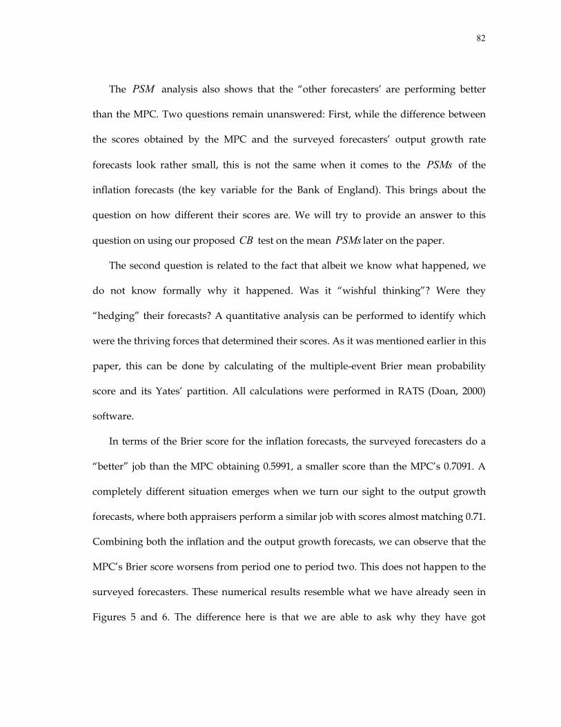
82

The PSM analysis also shows that the “other forecasters’ are performing better

than the MPC. Two questions remain unanswered: First, while the difference between

the scores obtained by the MPC and the surveyed forecasters’ output growth rate

forecasts look rather small, this is not the same when it comes to the PSMs of the

inflation forecasts (the key variable for the Bank of England). This brings about the

question on how different their scores are. We will try to provide an answer to this

question on using our proposed CB test on the mean PSMs later on the paper.

The second question is related to the fact that albeit we know what happened, we

do not know formally why it happened. Was it “wishful thinking”? Were they

“hedging” their forecasts? A quantitative analysis can be performed to identify which

were the thriving forces that determined their scores. As it was mentioned earlier in this

paper, this can be done by calculating of the multiple-event Brier mean probability

score and its Yates’ partition. All calculations were performed in RATS (Doan, 2000)

software.

In terms of the Brier score for the inflation forecasts, the surveyed forecasters do a

“better” job than the MPC obtaining 0.5991, a smaller score than the MPC’s 0.7091. A

completely different situation emerges when we turn our sight to the output growth

forecasts, where both appraisers perform a similar job with scores almost matching 0.71.

Combining both the inflation and the output growth forecasts, we can observe that the

MPC’s Brier score worsens from period one to period two. This does not happen to the

surveyed forecasters. These numerical results resemble what we have already seen in

Figures 5 and 6. The difference here is that we are able to ask why they have got

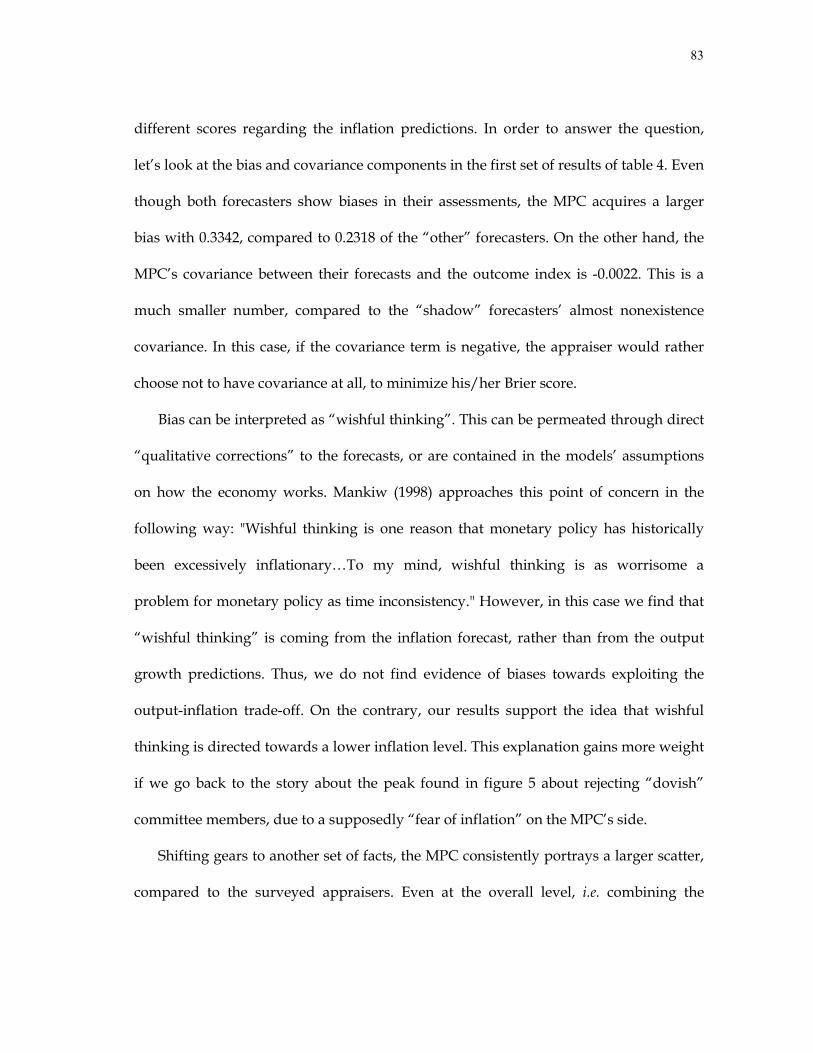
83

different scores regarding the inflation predictions. In order to answer the question,

let’s look at the bias and covariance components in the first set of results of table 4. Even

though both forecasters show biases in their assessments, the MPC acquires a larger

bias with 0.3342, compared to 0.2318 of the “other” forecasters. On the other hand, the

MPC’s covariance between their forecasts and the outcome index is -0.0022. This is a

much smaller number, compared to the “shadow” forecasters’ almost nonexistence

covariance. In this case, if the covariance term is negative, the appraiser would rather

choose not to have covariance at all, to minimize his/her Brier score.

Bias can be interpreted as “wishful thinking”. This can be permeated through direct

“qualitative corrections” to the forecasts, or are contained in the models’ assumptions

on how the economy works. Mankiw (1998) approaches this point of concern in the

following way: "Wishful thinking is one reason that monetary policy has historically

been excessively inflationary…To my mind, wishful thinking is as worrisome a

problem for monetary policy as time inconsistency." However, in this case we find that

“wishful thinking” is coming from the inflation forecast, rather than from the output

growth predictions. Thus, we do not find evidence of biases towards exploiting the

output-inflation trade-off. On the contrary, our results support the idea that wishful

thinking is directed towards a lower inflation level. This explanation gains more weight

if we go back to the story about the peak found in figure 5 about rejecting “dovish”

committee members, due to a supposedly “fear of inflation” on the MPC’s side.

Shifting gears to another set of facts, the MPC consistently portrays a larger scatter,

compared to the surveyed appraisers. Even at the overall level, i.e. combining the

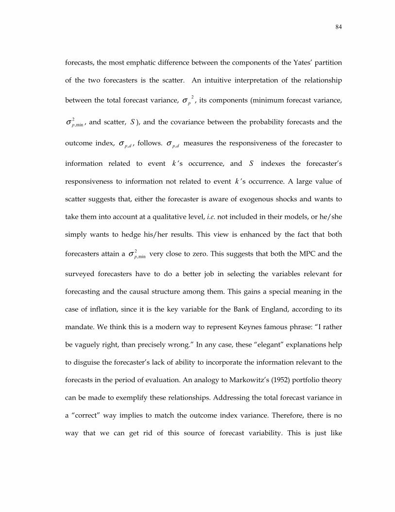
84

forecasts, the most emphatic difference between the components of the Yates’ partition

of the two forecasters is the scatter. An intuitive interpretation of the relationship

between the total forecast variance, 2pσ , its components (minimum forecast variance,

2min,pσ , and scatter, S ), and the covariance between the probability forecasts and the

outcome index, dp,σ , follows. dp,σ measures the responsiveness of the forecaster to

information related to event k ’s occurrence, and S indexes the forecaster’s

responsiveness to information not related to event k ’s occurrence. A large value of

scatter suggests that, either the forecaster is aware of exogenous shocks and wants to

take them into account at a qualitative level, i.e. not included in their models, or he/she

simply wants to hedge his/her results. This view is enhanced by the fact that both

forecasters attain a 2min,pσ very close to zero. This suggests that both the MPC and the

surveyed forecasters have to do a better job in selecting the variables relevant for

forecasting and the causal structure among them. This gains a special meaning in the

case of inflation, since it is the key variable for the Bank of England, according to its

mandate. We think this is a modern way to represent Keynes famous phrase: “I rather

be vaguely right, than precisely wrong.” In any case, these “elegant” explanations help

to disguise the forecaster’s lack of ability to incorporate the information relevant to the

forecasts in the period of evaluation. An analogy to Markowitz’s (1952) portfolio theory

can be made to exemplify these relationships. Addressing the total forecast variance in

a “correct” way implies to match the outcome index variance. Therefore, there is no

way that we can get rid of this source of forecast variability. This is just like

85

Markowitz’s “market” risk. Portfolio theory tells us that diversification, i.e. buying

stocks with a low correlation among them, can help to reduce the idiosyncratic (or

unique) risk and, as a result, decrease the overall risk. In this case, conducting efficient

research on the relevant information affecting the variables to be forecasted, such as

diversifying by using different models that capture different aspects of the economy,

will decrease the forecaster’s responsiveness to information not related to the forecast.

Consequently, this will improve the forecaster’s talent to discriminate between the

events that occur and the ones that did not occur, i.e. this will reduce the idiosyncratic

risk. Thus, minimize the Brier score. Summarizing, a large value of scatter suggests a

revision of the models and ideas used for forecasting purposes.

Notice that we propose to diversify, not to hedge. The second and third definitions

of the word “hedge” on the Merriam-Webster’s Dictionary (1994) are: ”means of

protection or defense (as against financial loss)”, and “a calculatedly noncommittal or

evasive statement”. The second definition of the word “diversification” is: ”to balance

(as an investment portfolio) defensively by dividing funds among securities of different

industries or of different classes”. We are sure that “calculatedly noncommittal“ and

“evasive statement” are not the phrases central banks want to be associated with.

A graphical approach to see each forecaster’s ability to discriminate between events

that occur and events that does not occur with more clarity is depicted in figure 8.

Figure 8 shows the covariance graphs of the probability judgments of the MPC and

the “other” forecasters for inflation and real GDP growth. We are able to observe

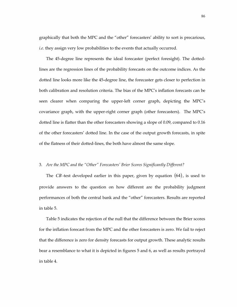
86

graphically that both the MPC and the “other” forecasters’ ability to sort is precarious,

i.e. they assign very low probabilities to the events that actually occurred.

The 45-degree line represents the ideal forecaster (perfect foresight). The dotted-

lines are the regression lines of the probability forecasts on the outcome indices. As the

dotted line looks more like the 45-degree line, the forecaster gets closer to perfection in

both calibration and resolution criteria. The bias of the MPC’s inflation forecasts can be

seen clearer when comparing the upper-left corner graph, depicting the MPC’s

covariance graph, with the upper-right corner graph (other forecasters). The MPC’s

dotted line is flatter than the other forecasters showing a slope of 0.09, compared to 0.16

of the other forecasters’ dotted line. In the case of the output growth forecasts, in spite

of the flatness of their dotted-lines, the both have almost the same slope.

3. Are the MPC and the “Other” Forecasters’ Brier Scores Significantly Different?

The CB -test developed earlier in this paper, given by equation ( )64 , is used to

provide answers to the question on how different are the probability judgment

performances of both the central bank and the “other” forecasters. Results are reported

in table 5.

Table 5 indicates the rejection of the null that the difference between the Brier scores

for the inflation forecast from the MPC and the other forecasters is zero. We fail to reject

that the difference is zero for density forecasts for output growth. These analytic results

bear a resemblance to what it is depicted in figures 5 and 6, as well as results portrayed

in table 4.

87

These results suggest that the MPC either attaches a certain degree of “wishful

thinking” to their inflation forecasts or hedges its inflation forecasts by adding extra

variability, or both. Results on table 4 provide evidence that both things happened

during the period under study. This explains the statistically significant difference

between the two Brier scores in the case of the inflation forecast.

E. Conclusions

Central bankers’ long-dated tradition of secrecy has been gradually going out of

fashion as many monetary authorities are convinced that transparency enhances

monetary policy’s stabilization performance. Several central banks have adopted more

transparent regimes; such is the case of inflation targeting. Others have gone even

further and now publish their inflation forecasts periodically. Bank of England (BoE)

does the latter. Their Monetary Policy Committee (MPC) has been informing the public

about their (as well as others’) future perspectives of inflation in a probabilistic sense,

on a quarterly basis.

In order to have the central bank’s monetary policy decisions accountable, optimal

forecast evaluation becomes an issue. While many studies use point-forecast techniques

to evaluate the MPC issued forecasts (for example, Pagan, 2003), some others have

recently utilized calibration-based evaluation methods (Wallis, 2003, 2004; Clements,

2004). Although calibration procedures are more appropriate forecast-evaluation

mechanisms -due to the probabilistic nature of their published forecasts-, they fail to

88

take into account the forecaster’s ability to sort between the events that occurred and

the events that did not occur.

We suggest central banks to publish their inflation forecast. Moreover, we

encourage them to do it in a probabilistic form. This is recommended in order to

provide the public with a complete probabilistic statement assessing the “upside” and

“downside” risks of future inflation, perceived at the moment prediction. On the other

hand, we suggest publishing forecasts from another sources or “shadow” forecasters.

The point that we emphasize is to evaluate these density forecasts calculating the

Probability Score for the latest forecast issued, as well as an overall performance

measure, such as the multiple-event version of the Brier mean probability score, along

with the Yates’ partition.

This paper presents an incentive-compatible approach to evaluate density forecasts.

Moreover, this line of attack offers means to extract important information about the

forecaster beliefs. This is presumed to alleviate the central banks’ accountability

problem and, potentially bolster monetary policy’s stabilization features. This is

achieved calculating the Yates’ partition (Yates, 1982) of the Brier Score (Brier, 1950) on

the MPC and “others’” forecasters on inflation and output.

Calibration only takes into account the reliability or ex post relative frequency of the

forecast, overlooking the resolution or ability to sort between outcomes that occurred

and did not occur. The Brier score encompasses the covariance between the realized

values and the forecast being a broader indicator. It is important to evaluate a central

bank because of their accuracy and sorting ability, rather than only by their calibration.

89

Utilizing these methodologies to evaluate the MPC and the surveyed forecasters’

inflation and output growth rate forecasts, we found the following three results. First,

our results indicate that both the MPC and the “other” forecasters have shown a large

responsiveness to information not related to the forecasted variable and a very

precarious response to developments affecting inflation and output growth. This

analysis insinuates that the MPC could be hedging its forecasts.

Second, “wishful thinking” in monetary policy has been usually identified as a bias

towards the exploitation of the short-run output-inflation tradeoff. Conversely, our

results indicate the MPC has been promoting its “wishful thinking” through its

forecasts more on the “fear of inflation” side.

Third, while there is not a statistically significant difference between the Brier mean

probability scores for the output growth forecasts, there is a significant one for the

inflation forecast. This supports the ideas that the MPC could be hedging their inflation

forecasts and, at the same time, influencing them with “wishful” thoughts against a

high-inflation (perhaps even moderate) outcome.

We can see that BoE uses the forecast as an instrument. But publishing a true

forecast, perhaps strips the power off the forecast as an instrument, but gives more

power to monetary policy itself, since the public will improve predictability of

monetary policy and their actions will reflect better behavior ad hoc with monetary

policymaking decisions. In other words, this could be seen as a transfer of power from

one instrument to another or just emphasizing the usefulness of the instrument, in this

90

case, by encouraging honesty on the publication of the forecast, will be emphasize the

open-market operations to set the key interest rate, monetary policy literally.

Regarding the incentive-compatible feature of the Brier score, it has been thought

that the scoring rule proposed by Brier could be used in the context of a contract

between the govt. and the central bank a la Persson and Tabellini (1993, 1999, 2000) and

Walsh (1995a, 1998). But, although we do recognize that their work has been useful to

understand certain issues in modern monetary policymaking from a theoretical point of

view, there are certain ambiguities that come into sight from try to apply this approach

to central banking (Blinder, 1998). Hence, this possibility was discarded.

The use of Brier score belongs to a so-called decision-based approach to evaluate

forecasts. Clements (2004) calculates decision base theory rules and concludes the same

as Wallis (2003, 2004). There are criticisms with respect to the use of these criteria for

forecast evaluation (Pesaran and Skouras, 2002; Wallis, 2004). Wallis states that,

although decision theory states that all forecasts should be evaluated in terms of the

gains and losses that resulted from using the forecasts to solve a sequence of decision

problems, macroeconomics forecasts are published for the general use and we have

little knowledge on the users’ specific decision contexts and evaluation. Nevertheless,

aggregation of the preferences of individuals across the economy makes this task an

impossible one. Our focus is more into evaluation the forecast to ensure an optimal

degree of transparency by making the central bank accountable of their actions, via

their forecast. We not only propose to encourage the central bank to be honest in their

91

forecasting reports, but also to persuade the monetary policy committees to exert their

best effort when constructing their forecasts.

Granger (2001) states that forecast evaluation criteria depend on the purpose of the

forecast. Along the same lines as Granger, we are integrating central bank’s

transparency as a beneficial feature for both the central bank (forecast producer), and

the public (users), and accountability via a reputation-building mechanism that

encourages honesty and accuracy utilizing the Probability Score and the Brier

Probability Score.

The Brier score is said to work only for unconditional forecast evaluations. In a

context of evaluating forecast densities of output growth and unemployment, Clements

and Smith (2002) mention that this could be a potential problem. Clements (2004) and

Wallis (2003, 2004) discuss that the one-year-ahead forecasts can be treated as

unconditional forecasts since interest rates do not have such an impact on inflation in

the short-run. However, due to the lack of consistent one-year-ahead forecasts issued by

the external surveyed forecasters –published in the Inflation Report-, we focus our

analysis on the two-year-ahead forecasts. Clements and Smith (2002) conclude that

evaluating conditional forecasts with unconditionally-related forecast evaluation

techniques is not a major drawback if the data set is sufficiently small (that is our case)

and exploring better methods becomes worthwhile as the focus of the analysis lies on

larger data sets. On the more intuitive side, in our particular case, this could have

affected our analysis in the sense that central bank had more opportunity (time) not

only to act but to see the consequences of her actions and actually either be close to their

92

forecast if she places a large weight on “hitting” the forecast. On the other hand it could

have been far because the conditions of the economy change dramatically. This second

possibility can be ruled out by following the economic developments in the period of

analysis. In any case, this issue did not prevent us to arrive to the same conclusions as

Pagan (2003), Wallis (2003, 2004) and Clements (2004) that the MPC is “upwardly”

biased by placing too much probabilities to the high state precluding the less

conservative members of the Committee to gain any sympathy for rate cuts. On the

other hand, the evaluating the two-year density forecasts is important since longer term

forecasting horizons are usually related to the establishment of central bank credibility.

This fact suggests that future research should be undertaken in this topic. In the

specific case of the Bank of England, obtaining a “good” number of one-year-ahead

density forecasts by “other” forecasters in order to overcome the issue on

conditionality.

The MPC has changed their target from RPIX to the Consumer Price Index (CPI), it

could be interest in extending the analysis we propose in this paper to the CPI, once a

consistent and “decently” large number of observations becomes available.

Another topic is left out of the scope of the present research effort future research

would be to explore ways to relax assumption of neutrality of the forecaster with

respect to the forecast and its implications, if we believe that this is a strong

assumption. Henceforth we have noted quite a few topics for future research.

93

CHAPTER IV

WHAT CAUSES THE SACRIFICE RATIO?

Our inferences . . . always retain more or less of a hypothetical character, and are so far open to doubt. Only in proportion as our induction approximates to the character of perfect induction, does it approximates to certainty. The amount of uncertainty corresponds to the probability that other objects than those examined may exist and falsify our inferences; the amount of information yielded by our examination; and the theory of probability will be needed to prevent us from overestimating and underestimating the knowledge we possess. ― Jevons, W. S. (1874), p. 263

A. Introduction

According to Benjamin Friedman, the relationship between output and inflation has

been a (if not the) central reason for doing monetary policy (Solow and Taylor, 1999).

But, while it is a well-known fact that low inflation is an advantageous state in the

economy (see Barro, 1996, and Feldstein, 1999a, for well-documented surveys), there is

also consensus that disinflationary policies cause short-run output losses46 (Romer and

Romer, 1989; Ball, 1994).

The assessments of the costs of disinflationary policies have used the concept of

sacrifice ratio defined as the costs in terms of unemployment or loss of output that must

be faced to achieve a reduction in inflation.

46 Blanchard (1997) and Zhang (2001) –among others- go even further and claim that these policies can have long-run effects.

94

There have been several attempts to estimate the sacrifice ratio in the literature.

These can be divided in two classes: constant over time (Okun, 1978; Gordon and King,

1978; and recently Cecchetti and Rich, 2001), and case-by-case (Ball, 1994; Bernanke, et

al., 1999; Sánchez, Seade, and Werner, 1999, among others). Ball’s technique remains as

the “standard” method since Cecchetti and Rich concluded that their estimates are

imprecise.

We take the “case-by-case” approach in this study. The numerator is the (discrete)

sum of the differences between the potential Gross Domestic Product (GDP), and the

realized GDP -also called output gap-, across the time periods within the disinflation

episodes. The denominator is the change in the inflation rate from the beginning to the

end of the identified disinflation episode.

We divide the variables that presumably affect the magnitude of the sacrifice ratio

into three categories: “traditional”, “structural”, and “institutional”. The set of

traditional determinants encompasses a series of variables that, on one hand, have been

“key” issues in the modern monetary macroeconomics debate for a long time. These are

also related to the sacrifice ratio in a more operative basis. The structural factors

incorporate the characteristics of the countries economic agents’ interactions, such as

wage rigidities and the degree of openness of the economy. The third set of

determinants is much of a newer one in the literature. The institutional aspect reflects

the need to account for the structure of incentives that are likely to be within the central

banks’ institutional structure. Such is the case of Central Bank Independence (CBI) and

Inflation Targeting (IT). These factors are out of the scope of Ball’s analysis.

95

In order to identify the impact of the determinants on the sacrifice ratio, the

literature has provided neither a formal theoretical framework, nor a consistent

empirical estimation technique to assess the way these factors affect the magnitude of

the sacrifice ratio. Scatter diagrams, simple correlations, and simple regressions have

been performed on empirical estimates of the sacrifice ratios, usually evaluating each

factor separately.

We believe that it is extremely important to identify the causal structure underlying

the sacrifice ratio and its determinants to achieve a more effective way of implementing

monetary policy. In order to succeed to provide the set of factors that can be

manipulated to reduce the costs of disinflation, we have to be able to recognize which

are and which are not the factors that affect the sacrifice ratios, in order to choose

“correct” variable and obtain the desirable outcome, if it is possible.

That is why we used a new tool that retrieves the causal structure from a set of

empirical observations. A methodological introduction to the techniques that are used

in this study follows. We believe that a simple and general algorithm for the

construction of empirical models can be summarized into four steps: 1. Select the

variables that we think are relevant for our abstraction of reality, the model, e.g. x , y ,

z ; 2. Set the relationships of the variables –namely- the causal structure, for instance

( )zxfy ,= which in this case implies that x and z cause y ; 3. Choose the functional

forms, let’s say, linear czbxay ++= , where a , b , and c are parameters; 4. Decide the

estimation method, least squares, generalized method of moments, and so on and so

forth. Economic theory is usually involved in steps 1, 2, and 3; econometric theory in 3

96

and 4. But what if theory has not provided a sensible and consistent theory on how the

variables are causally related. In other words, if step 4 is not fully analyzed or proven.

To emphasize the importance of performing a reasonable analysis in step 4, let’s say

that we think that the following causal structure YXZ →→ represents the truth. We

would be tempted to manipulate X to provoke an effect on Y . But what about if the

real causal structure is YZX →← ? Manipulating X will never have an effect on Y .

A handy example follows47. Assume that Z refers to smoking cigarettes, X stands for

yellow fingers, and Y is terminal cancer. If we prescribe a treatment for yellow fingers,

we will not be affecting terminal cancer. This point is supported by Hausman (1998)

when he says that manipulation is at the heart of causation. Trying to manipulate the

“wrong” variable could lead to an outcome different from the one that is desired.

There are two probabilistic approaches to estimate data-based causality: the

“celebrated” Granger causality (Granger, 1969), based on “incremental predictability,

and Directed Acyclical Graphs (DAG), a combination of graph theory48 with modern

artificial intelligence methods proposed by Pearl (1986, 2000) and Spirtes, Glymour, and

Scheines (1993, 2000). The former has been used extensively in the economic literature.

The latter has started to permeate the economic literature and has been used by Bessler

and Lee (2002), Bessler and Kergna (2002), Awokuse and Bessler (2003), Bessler and

Yang (2003), and Yang and Bessler (2002) to identify a causal structure whenever theory

fails to provide a sensible explanation of step 4 (above). Granger and Swanson (1997)

47 Pearl (2000)

48 See Maxwell and Reed (1971) for a comprehensive introduction to graph theory.

97

use a similar methodology to retrieve a causal structure from the residuals of a vector

autoregression (VAR).

Two reasons lead us to pick DAGs for the assessment of the determinants of the

sacrifice ratios. First, the episode-by-episode nature of the data. In other words, we do

not have a “continuous” stream of data. Therefore Granger causality cannot be used.

The other, and more powerful reason, is that DAGs is that Granger causality assumes

no contemporaneous correlations.

Instead of imposing an a priori structure, an empirically-based structure is sought

using Directed Acyclical Graphs (DAGs) (Pearl, 1986, 2000) and the PC Algorithm

(Spirtes, Glymour and Scheines, 1993, 2000). We utilize DAG analysis on quarterly data

from eleven member countries of the Organization for Economic Cooperation and

Development (OECD) for the 1960-2000 period. We find that there is evidence that

wage rigidities and central bank independence (CBI) are two major determinants of the

sacrifice ratio. This supports Ball’s (1994) results as well as other empirical analyses on

CBI such as Debelle and Fischer (1994), Walsh (1995b), Froyen and Waud (1995), and

Fischer, (1996). Although we find that openness is affected by CBI, we do not find

support for Romer’s (1993) view that it has an effect on the sacrifice ratio. This is in line

with a recent study by Temple (2002). Along the same lines as Bernanke, et al. (1999), we

do not provide a solid assessment on the relationship between inflation targeting (IT)

and the sacrifice ratio due to the recent adoption of these regimes and that our analysis

is restricted to disinflation episodes only, yielding very few observations.

98

This paper is innovative in three ways. (i) It extends Ball’s sacrifice ratio calculations

by including observations for the 1992-2000 period; (ii) It includes CBI and IT as

relevant variables to possibly explain the costs of disinflation; (iii) And most

importantly, it uses a new causal engine to determine the causal structure of the model

to estimate a regression based on the identified causal model.

The paper consists of five sections. The first section describes the methodology used

to calculate the sacrifice ratios, and presents estimates of the sacrifice ratios for eleven

OECD countries for disinflation episodes between 1960 and 2000. Section B discusses

the theoretically-based factors that are supposed to have and effect on the magnitude of

the sacrifice ratio. It also provides a description of the data used to examine each of

these factors. The third section offers a brief introduction to the Directed Acyclical

Graph approach at a theoretical level. Details about the results from past literature as

well as our findings are discussed in section E. Section F provides concluding notes.

B. Calculating the Sacrifice Ratios

1. The Sacrifice Ratio

The theoretical foundations of the sacrifice ratio are based on the expectations-

augmented Phillips curve (Phillips, 1958; Friedman, 1969a; Phelps, 1968), or Lucas

supply curve with backward expectations49 (Lucas, 1972, 1973):

49 In other words, using lag inflation as a proxy of expected inflation.

99

( )68 ( ) ( ) 10,0,111 <≤>+−+−=− ∗−−−

∗ βαεβππα ttttttt yyyy

where y is the (natural) log of real output, ∗y the log of potential output , π is the

inflation rate, ε is a disturbance term, α and β are parameters. Subindex 1−t

indicates the variable is measured at time 1−t , and t stands for a period ahead.

Disinflation occurs whenever 01 <− −tt ππ . The term ∗− tt yy is the output gap, or

deviation of output from its potential level, attributable to a disinflation policy at time

t . If disinflation does not occur ( 01 ≥− −tt ππ ), output ( y ) remains at its potential level

( ∗y ) if output was at its potential level in the last period. If disinflation takes place,

there is a short-term output loss. As α increases, the cost of disinflation gets larger.

Nevertheless, output reverts to its potential level in the long run. β is the persistence or

“long-lived” effect of the disinflation policy on the long-run output gap. In other words,

β determines how long it takes for the output to return to its potential level after a

disinflation policy occurred.

Although β reveals how strong (or weak) are the effects of the disinflation policy

on the output gap, it does not affect the potential (trend) output. An extreme case takes

place whenever these disinflation policies cause a permanent decline in unemployment

and output; this is defined as hysteresis (Blanchard and Summers, 1986). Blanchard

(1997) illustrates the hysteresis effect with the following equation:

( )69 ( ) 10,1 11 ≤≤+−+=− −∗−

∗ θθθ tttt yyyyy

where y is the constant growth rate for potential output, θ is the level of hysteresis

effect, and the other terms follow from the notation above. If 10 ≤< θ , there is a

100

hysteresis effect. And the sacrifice ratio becomes larger with the intensity of θ .

Whenever 0=θ , there is no hysteresis at all.

Attempts on estimating the sacrifice ratio fall into two categories: “constant-over-

time” estimation and “case-by-case” studies. The former methods were pioneered by

Okun (1978) who analyzed a set of Phillips curve models to estimate the cost of

disinflation in terms of the percentage loss of output during a given period. Gordon and

King (1982) derived the sacrifice ratio using both “traditional” and Vector

Autoregressive (VAR) models. More recently Cecchetti and Rich (2001) obtained

estimates of the sacrifice ratio utilizing Structural Vector Autorregressions (SVAR),

identifying aggregate demand and aggregate supply shocks a la Blanchard and Quah

(1989)50.

The “case-by-case” method was developed by Ball (1994). Ball explored this new

approach motivated by the two limitations of the methodologies described above. On

one hand, they constrain the estimated ratios to be identical for disinflation periods as

for periods of increasing trend-inflation or short-run aggregate demand fluctuations.

On the other hand they constrain the sacrifice ratios to be constant over time. These two

restrictions neglect the facts that disinflations are influenced by disinflation-specific

factors (such as credibility shifts in expectations), and, time-specific institutional factors

(such as labor contract structures or the degree of openness of the economy –among

others).

50 Model “C” in Amisano and Giannini’s (1997) generalized SVAR approach.

101

Ball’s technique has received criticism from Friedman (1994) and Cecchetti (1994) on

the basis of using foregone output instead of rise of unemployment as the loss criterion,

and ignoring the “benefits” from loosening monetary policy as well as the likely

existence of supply shocks, respectively. Despite these criticisms, Ball’s methodology

has become a “standard” in the field and has been used by numerous recent studies

(Jordan, 1997; Bernake, Laubach, Mishkin, and Posen, 1999; Sánchez, Seade, and

Werner, 1999; Zhang, 2001; Çetinkaya and Yavuz, 2002; Temple, 2002; and Boschen and

Weise, 1999, 2003). We believe that this is because Ball provided a fairly uncomplicated

methodology whose estimates are consistent with the “traditional” inflation-output

literature, as well as because of the mentioned limitations of the constant-over-time

approach and Cecchetti’s (2001) severe self-criticisms on his SVAR derived estimates:

“…the estimates are very imprecise, which we suggest reflects the poor quality of

instruments used in estimation. We conclude that the estimates provide a very

unreliable guide for assessing the output cost of disinflation policy.”

Using the best methodology available to estimate the sacrifice ratios is a necessary

condition for a good assessment on the factors that presumably affect them. As a result,

Ball’s methodology is used in this paper.

Ball’s definition of the sacrifice ratio ( SR ) is the following:

( )70 ( )π∆

−=∑∈

∗

Dttt yy

SR

where the numerator is the output gap, i.e. the (discrete) sum of the differences between

the realized GDP ( ty ) and the potential GDP ( ∗ty ), across the time periods within the

102

disinflation episode ( Dt∈ ). The denominator is the change in the inflation rate from

the beginning to the end of the identified disinflation episode. SR is interpreted as the

cost of reducing one percentage point of inflation in terms of aggregate demand

contraction, which is similar to α , in equation ( )68 .

The construction of this estimate for the sacrifice ratio has two underlying

assumptions: ignores supply shocks –criticized by Cecchetti (1994)- and presumes that

there is no hysteresis, i.e. 0=θ in equation ( )69 . The first assumption introduces noise

to the sacrifice ratio estimation as a measure of the inflation-output trade-off. Along the

same lines as Ball (1994, pg. 161), we claim that these measurement disturbances will be

reflected in the regression errors and will not cause a major problem in our analysis. On

the hysteresis effect, Zhang (2001) studies the potential downward bias in calculating

the sacrifice ratio whenever hysteresis is neglected51. There is almost consensus that

there are short-run effects of disinflation policies, but there is still considerable debate

on its long-run effects. The focus of this study is the short-run effects of disinflationary

policies, as a result, we maintain Ball’s assumptions (as other authors mentioned

above).

2. Identifying Disinflation Periods and the Measurement of the Output Gap

The methodology proposed by Ball consists of two steps: identify the disinflation

episodes ( D ), and calculate ( )∑ ∈∗−

Dt tt yy , the departure of real output from its

51 Zhang (2001) also studies the importance of accounting for the effects of persistence –namely β in equation (68)- “correctly”. We assess the persistence assumption later in the paper.

103

potential level during D . The former intends to separate the small fluctuations (arising

from ”exogenous” shocks) from the relevant policy-induced changes in inflation. The

latter is the heart of the sacrifice ratio.

A series of basic characterizations used by Ball follows. In order to identify the

disinflation periods, a smoothed version of inflation or “trend inflation” ( Ttπ ) is

calculated as a centered, eight-quarter moving average of actual inflation.

( )71 ∑+

−+=

it

itt

Tt i

ππ12

1

where i is an index. Although there are data on inflation for the whole sample, output

data is only available on an annual basis, as a result, 4=i for the quarterly data trend

inflation, and 1=i for the annual data. Therefore, the annual data trend inflation is

defined as a two-year centered moving average of realized inflation.

In any given country, a disinflation period starts (ends) on the “peak” (‘trough”),

defined as the point in time where trend inflation is higher (lower) than the previous

and the next 4 quarters (for quarterly data), and 1 year for annual data.

Ball identifies twenty-eight disinflationary periods in nine countries, using quarterly

data and sixty-five episodes in nineteen countries, with annual data.

The most delicate subject concerns the measurement of the output gap, due to the

fact that there is no general agreement among economists on how to assess this issue.

Ball departs from the most used methodology to calculate the trend output, the

Hodrick-Prescott (HP) filter (Hodrick and Prescott, 1980, 1997) due to the fact that the

filtered trend output follows the realized output very closely, practically eliminating the

104

differences between them, as a result, this eradicates any possibility of accounting for

recessions. Instead, Ball assumes the following: (i) Real output is at its potential level at

the beginning of the disinflation episode; (ii) Output reverts to its “natural” level four

quarters (one year) after the trough52; (iii) Trend output grows log-linearly between the

peak and the four quarters (one year) after the trough.

Figure 9 shows graphically the methodology of calculation of the sacrifice ratio on a

“case-by-case” basis.

Assumptions (i) (i.e. Dttt yy

inf=

∗= ) and (iii) (i.e. log-linearity of trend output) have

not been challenged to a large extent. But supposition ii has attracted modest debate

(Blinder, 1987; Romer and Romer, 1989, 1994). Particularly, Zhang (2001) argues that

there is a downside bias in the measurement of the sacrifice ratio if the methodology

neither accounts for persistence effects in a “correct” fashion, nor includes hysteresis

effects. Despite these critiques, as we mentioned above, given that we are interested in

the short-run effects of this policies and there is not yet a general agreement on the

existence of strong persistence effects or even hysteresis, we rule out these two factors.

3. Estimates of the Sacrifice Ratio

Ball estimated sacrifice ratios using quarterly and annual data. We analyze the

determinants of the sacrifice ratio on quarterly data because we are only interested in

52 Thus, the ordered elements of set D (the dates) are the date of the peak (start), four quarters (or one year) after the trough (end), and the dates between these two. Translating this assumption into equations (1) and (2) is as if β in the fourth quarter, after the trough, approximates to zero. Moreover, assumes no hysteresis (i.e. θ=0).

105

the short-run fluctuations and using annual data dampens short-run inflation

movements. We believe this has been the rationale behind the use of quarterly, rather

than annual data in the majority of the studies mentioned earlier in the paper.

We took the sacrifice ratio estimates from Ball’s quarterly data on 9 countries

(Australia, Canada, France, Germany, Italy, Japan, Switzerland, United Kingdom, and

United States), and added information for two more OECD countries relevant to

address inflation targeting: Sweden and New Zealand. Additionally, we updated the

sample for the 1990-2000 period using the Ball’s methodology on data obtained from

the same source of information, the International Monetary Fund’s (IMF) International

Financial Statistics (IFS). Ball acknowledged 28 disinflation episodes, we identified 15

additional disinflation periods, 11 of them occurred in the 1990-2000 decade53.

Estimates for the sacrifice ratios along with their respective episode

characterizations are shown on Table 6. In addition the table presents corresponding

measures of initial inflation, change in inflation, length of disinflation, and speed of

disinflation, all calculated as in Ball (1994). Speed of disinflation is defined as the

quotient between the change of inflation and the length of the disinflation event, i.e.

how many inflation percentage points were diminished in a quarter of a year.

There are eight positive and thirty-five negative sacrifice ratios. A negative sacrifice

ratio reflects that the economy grew at a higher rate than the trend, despite that a

disinflation policy was implemented during that period. We do not think this

53 We compared our estimates with the ones provided by Sánchez, Seade, and Werner (2001) who used Ball’s methodology on IFS data, and there are exactly the same.

106

contradicts the widely accepted view that disinflation policies cause output losses, since

the presence of positive sacrifice ratios represents less than a quarter of the sample.

The average sacrifice ratio is 1.14 with a standard deviation of 1.18. In other words,

it costs 1.14 percentage points of GDP growth rate to reduce one percentage point in

inflation, on average. On the other hand, differences across countries are considerable.

The United States possesses the highest costs of disinflation, estimated by the sacrifice

ratio, with an average of 2.71 across its four identified disinflation episodes, followed by

Germany with an average of 2.38. These two results are in line with Ball’s findings in

spite of updating the sample. Sweden and New Zealand figured as the countries where

disinflation policies are less costly, with 0.46 and a negative 0.23 mean sacrifice ratios,

respectively. In the case of average initial inflation, France and New Zealand positioned

themselves in the first two places with corresponding average inflation levels of 16.6

percent and 12.5 percent. On the other hand, on average, Switzerland and Germany

started with the lowest inflation levels of about 7.12 percent and 5.4 percent, in that

order. Moreover, while New Zealand and Japan achieved the highest average speeds in

reducing inflation with 0.60 and 0.56 inflation points per quarter, respectively, the

“speedometer” showed that Germany and Canada took unhurried actions to diminish

inflation with speeds corresponding to 0.27 and 0.32 inflation points per quarter. By

relating these estimated sacrifice ratios with their average speeds, it might lead us to

think right away that there is an inverse relationship between these two variables. In

other words, that it is more costly to reduce inflation in a slow fashion. This has strong

implications in the modern macroeconomic debate because this asseveration would

107

support Sargent’s (1983) arguments and, at the same time, defeat Taylor’s (1983)

gradual approach, a consequence of his staggered-price model54. However, this is a

preliminary appraisal of the historical correlation between these two variables, and not

a causal analysis. Our analysis (on section E) will try to provide an answer to this as

well as other related questions. Furthermore, despite of the high-speed achieved by

New Zealand, it took their monetary authority 26 quarters to reduce inflation 15.62

percentage points. For the central banks of Japan and the United Kingdom it only took

an average of 11 quarters, but they reduced only 4.5 and 6 percentage points,

respectively.

Table 7 portrays summary statistics by decade. The first result that stands out is that

the average sacrifice ratios show a decreasing trend. At first sight, this seems to be good

news, but identifying the main cause of this encouraging result is not an easy task. This

is because we have relationships that that are not consistent across time (at this simple

level of the analysis), as well as the fact that we have not accounted for other factors

that could be of relevance to this phenomenon, such as the trend to increase the degree

of central bank independence or the adoption of inflation targeting –among others-.

Another set of facts that are reflected in table 7 is that it seems that reducing

inflation was more popular during the eighties. Compared to the three other decades,

14 disinflation episodes were identified with an average reduction of 7.8 percentage

points in inflation each, during the 1980-1990 decade. This is a situation that clearly did

54 Section C provides a wider discussion on this debate.

108

not happen during the sixties when central bankers still tried to exploit the seemingly

downward-sloping Phillips curve.

Shifting gears to the initial inflation-sacrifice ratio relationship, it is not a clear that

the costs of disinflation are lower at higher levels of initial inflation. This is because the

average initial levels of inflation in the sixties as well as in the nineties are around 5.6

percent, and the corresponding average sacrifice ratios are mixed outcomes of 1.7 and

0.6.

We also observe that the monetary authorities hurried up to decrease inflation

levels with an average speed of half of a point per quarter during the sixties, seventies,

and eighties, taking them on average 8, 11, and 18 quarters, respectively, to reduce

inflation at the “desired” levels. It took longer periods of time in the seventies and

eighties perhaps due to the fact that there were larger differences between inflation

levels at the beginning of the disinflation episode and the central bank’s targeted levels.

C. Determinants of the Sacrifice Ratio

This section presents the relevant theoretical variables that are suggested in the

literature to have a meaningful effect on the magnitude of the sacrifice ratio. It also

describes the data that are used to examine each of these factors.

109

1. Traditional Factors

Factors such as the speed of disinflation, and the inflation rate at the beginning of

the disinflation periods are more closely related to the more “traditional” operational

view of monetary policymaking.

One of the most widespread controversies in modern macroeconomics is the choice

between gradualism or quick disinflation and its impact on real output. An argument in

favor of taking a gradual approach towards dampening inflation is supported by Taylor

(1983). He prescribes a steady but slow decline in inflation in the light of a staggered-

wage adjustment model for the reason that wages and prices need time to adjust to a

monetary contraction, linking quick disinflations to large output losses.

Conversely, there are two different major views on this issue. Along the same lines

of the NeoKeynesian price stickiness hypotheses, the celebrated “menu cost” approach

supports a quick disinflation rather that a gradual one. This is because a once-and-for-

all large shift in inflation will yield adjustment of prices and will not affect output

significantly. In contrast, a series of small changes in inflation will provoke output

losses.

The other argument that favors a quick disinflation is due to Sargent (1983). He

claims that blunt regime shifts provide credibility to the monetary authority, while for

gradual shifts (or slowly changing policy), expectations do not adjust because

speculation about what will happen next emerges.

Unfortunately, there is not an unambiguous empirical characterization of the speed

of disinflation. If we maintain the basic definition of average speed in physics (the

110

distance traveled divided by the time taken to travel that distance), we end up

calculating the (absolute) difference of the inflation rates between the initial and the end

of the disinflation period as the numerator, and the length of the disinflation period as

denominator. The theoretical dilemma is that while Taylor’s approach suggests that the

sacrifice ratio is only influenced by the length of the disinflation period (denominator),

Sargent’s analysis focuses on the numerator as the key element of the quotient, since a

large change in inflation is probably taken more seriously as a regime change. Ball

recognizes this issue by running regressions on both, the speed of disinflation in the

physics canonical form and with its separate components. He finds that regardless of

which specification, quicker disinflations produce lower sacrifice ratios. Sánchez, Seade,

and Werner (1999) use the speed metric as well on a larger sample and conclude the

same as Ball. Temple (2002) uses the length of disinflation and the inflation rate change

and, although it is not the focus of his study, he arrives at the same conclusions.

The second traditional factor is the initial inflation. NeoKeynesian models predict

that higher inflation levels decrease the degree of price rigidities. Ball, Mankiw and

Romer (1988) derive this initiative theoretically and find empirical support on cross-

country analyses. In other words, when there is a large rise in prices in a short period of

time, businesses need to “keep up” with the pace of inflation and stickiness is reduced.

Therefore, following this raison d'être, initial inflation should show a negative

relationship with the sacrifice ratio.

111

2. Structural Factors

Nominal wage rigidity stands as the oldest institutional determinant identified to

have potential effect on the sacrifice ratio. Even though, the latest NeoKeynesian

convention emphasizes the role of output-price stickiness, rather than wage-related

rigidities (Mankiw, 1990), Ball’s rationale, which we adopt in this paper, is more a

practical one. He utilizes two different measures of nominal wage rigidities as a proxy

of price stickiness and investigates their relationship with the sacrifice ratio. These two

measures are the Bruno and Sachs (1985) index of wage responsiveness, henceforth

B&S, and the Grubb, Jackman, and Layard (1983) index of overall wage rigidity, or GJL

index. The former metric (B&S) is constructed adding the degree of wage indexation

and synchronization to the index of duration of wage agreements. The B&S index

ranges from 0 to 6, and a smaller value means a more rigid wage structure. The GJL

index is build upon a time-series regression of wages on unemployment and prices. The

average GJL index for our sample is 0.7, ranging from 0.09 for the country with the

most flexible wage structure (Switzerland) to 3.14, corresponding to the country with

the least flexible wage structure (United States). As Ball explains, while GJL is less

subjective compared to the B&S index, it is an endogenous metric since the traditional

factors are directly involved with the components of the GJL index.

Basic open-macroeconomic theory recognizes that the degree of openness of an

economy keeps an inverse relationship with the output losses related to disinflation

policies (Romer, 1993). This is because a monetary contraction produces an exchange

rate appreciation, having an effect on prices to the extent of the degree of openness of

112

the economy55. The most widely used metric is the proportion of the imports of GDP,

calculated by Romer (1993). Switzerland figures as the most opened country in our

sample whose imports represent approximately 35 percent of their GDP. Conversely,

the United States’ imports only account for 9 percent of their GDP. The average

percentage across the sample is 22 percent.

Ball and more recently Temple (2002) conclude that there is no strong evidence of

an effect of the degree of openness of an economy on the slope of the output-inflation

tradeoff. Nevertheless, Daniels, Nourzad, and VanHoose (2004) analyze Temple’s data

and find an “unambiguous positive relationship between openness and the sacrifice

ratio”, once they account for the degree of Central Bank Independence (CBI) and its

interaction with openness itself. CBI is discussed in the next subsection.

3. Institutional Factors

We next turn to institutional factors. These variables reflect the need to account for

the structure of incentives that are likely to be within the central banks’ institutional

structure. First we consider Central Bank Independence (CBI), defined as the

assignment of monetary policy to a central banker whose decisions cannot be rejected

by the policymaker (Lippi, 1999). Herrendorf and Neumann (1999) claim that a

55 As far we know Sánchez, Seade, and Werner (1999) are the only authors who have included the exchange rate regime as a possible determinant of the sacrifice ratio. They are motivated by the fact that if an economy is sufficiently open, the exchange rate variability has a larger effect on domestic prices. A non-floating exchange rate system constrains the variability of the relative prices between nations. Thus, this could have direct effects on the inflation-output tradeoff. On one hand, this issue can be (at least) partially accounted for in the inclusion of the measurement of the degree of openness of the economy. On the other hand, finding an objective metric for this issue is not an easy task, therefore we leave this interesting question out of the scope of this study for future research.

113

politically-detached (independent) central bank exhibits less incentive to care about the

government’s reelection chances, reducing the possibility of using monetary policy to

create surprise inflation.

Several efforts have been directed to measure the degree of CBI and its relationship

with both nominal and real variables such as inflation and real output. Most of this

literature pioneered by Bade and Parkin (1984), has been surveyed by Cukierman (1992)

and Eijffinger and de Haan (1996). The most widely used metric is the legal-based index

by Cukierman, Webb, and Nayapti (1992). This index is composed of four categories:

(i) CEO variables (term of office, who appoints, etc.), (ii) policy formulation variables

(who formulates, final authority, role in budget), (iii) central bank objectives. And (iv)

Limitations on lending variables (type of limit, maturity of loans, terms of lending, etc.).

The Cukierman, et al. CBI index ranges between 0.18 (Japan) and 0.69 (Germany) in our

sample. As the number approaches unity, the central bank enjoys a larger degree of

independence. Except for United Kingdom and Switzerland, the calculated indices for

each country in our sample show no variation across time. Therefore, variability is

observed in a cross-country basis.

Various studies have reported positive and significant correlation between CBI and

the sacrifice ratio (Debelle and Fischer, 1994; Walsh, 1995b; Froyen and Waud, 1995; and

Fischer, 1996). The most common theoretical explanation behind these empirical results

is that CBI might help to diminish the levels of inflation, by reducing the inflation bias

incentives. However, it could also increase the nominal wage rigidities indirectly,

intensifying the magnitude of the sacrifice ratio (Walsh, 1995b).

114

The second institutional factor in our proposed taxonomy is Inflation Targeting (IT).

Bernanke, et al. (1999, pg. 4) define IT as “…a framework for monetary policy

characterized by the public announcement of official quantitative targets (or target

ranges) for the inflation rate over one or more time horizons, and by explicit

acknowledgement that low, stable inflation is monetary policy’s primary long-run

goal.”

Since the adoption of IT has been fairly recent and our sample is constrained to

disinflations periods only, our analysis on this issue is rather cautious. We identified six

episodes in countries that have already adopted IT by the time of the occurrence of the

disinflation period. Nevertheless, in certain cases the adoption of IT took place in the

midst of a disinflation episode. Consequently we define IT as the number of quarters

that IT was active within the disinflation episode, divided by the length of the

disinflation period itself, yielding a number ranging between zero and one. The average

from these six observations was 0.60, with a standard deviation of 0.36. In other words,

countries observed IT in approximately 11 of the 18 quarters that the disinflation

episodes lasted, on average.

While CBI is likely to provide a larger degree of discretion to central banks,

adopting IT constrains them to observe a certain level of inflation. This constrained

flexibility is desirable since despite the view that monetary policy cannot systematically

affect unemployment and output in the long-run, it might aid to stabilize inflation and

unemployment around mean market-determined levels (Fischer, 1977).

115

Another theoretical argument in the spirit of the dynamic inconsistency literature

on why a country adopting an inflation targeting regime should have a smaller sacrifice

ratio, is that IT minimizes the central banks’ incentives to exhibit an opportunistic

behavior (inflation bias) and this might increase the central banks’ credibility and, as a

result, the public moderates their inflations expectations in a quicker fashion.

However, it could be the other way around, if the central banks’ focus centers on

inflation objectives only, nominal wage indexation could be reduced, increasing the

nominal wage rigidity and the sacrifice ratio as well (Walsh, 1995b).

Bernanke, et al. (1999) find that the estimated sacrifice ratios for three of the four

surveyed countries that adopted IT is higher than before the implementation of such

regime. This suggests that the adoption of IT has not reduced he costs of disinflation.

Furthermore, they suggest that this regime change has even increased them.

Nevertheless, they acknowledge that these results are somewhat weak because of the

limitations imposed by the small sample of countries and period of time since their

adoption of IT. Only recently have countries adopted IT: New Zealand, 1990; Canada,

1991; U.K., 1992; Australia, 1993; Sweden, 199356.

D. Empirically-Based Causal Structure

The theoretical foundations of Directed Acyclical Graphs (DAG) as a probabilistic

approach to infer causality from a data set have their origins in Pearl (1986). Combining

56 More recently Brazil, Mexico, Czech Republic, Hungry, Korea, Peru, Poland, and Thailand have adopted an Inflation Targeting regime.

116

the traditional philosophical notions of causality with statistical theory, Pearl proposed

the concept of d-separation (defined in Pearl, 2000, pp. 16-17.), to describe conditional

independence with a graphical approach57.

Spirtes, Glymour, and Scheines (1993, 2000) developed algorithms based on

Artificial Intelligence (AI), integrating the concept of d-separation to retrieve the causal

structure from empirical data. Their main contribution: a search-theoretic algorithm

called the PC algorithm.

Although this approach was born on the fields of Philosophy, Statistics, and

Computer Science, it has now been increasingly used in economics and finance.

Swanson and Granger (1997) pioneered in the application of DAGs in a Vector

Autoregression setting. Bessler and Lee (2002), and Awokuse and Bessler (2003) apply

these ideas to recent macroeconomic VARs. Demiralp and Hoover (2003) judged the

usefulness of the PC algorithm using Monte-Carlo simulations to test how close the

causal structure inferred by this methodology was from the data generating process’

true causal system. They found very encouraging results.

We utilize the directed acyclical graph conceptual framework as well as the PC

algorithm with cross-section data (as originally proposed by Spirtes, Glymour, and

Scheines, 2000). This is because we are dealing with not necessarily time-sequenced

disinflation episodes across several countries.

57 A proof of this proposition can be found in Verma and Pearl (1988).

117

1. Directed Acyclical Graphs

This part relies heavily on the work by Pearl (2000) and Spirtes, Glymour and

Scheines (1993, 2000). A directed graph is formally defined as an ordered triple

EMV ,, , where V is a nonempty set of vertices (variables), M is a non-empty set of

marks (symbols attached to the end of undirected edges; e.g., > or < ), and E is a set of

ordered pairs (the lines between them). In other words, directed graphs are pictures

summarizing the causal flow among a set of variables.

A directed acyclic graph (DAG) is a directed graph that contains no feedback cycles.

In other words, cyclic graphs such as ACBA →→→ , assuming a set of vertices

(variables) { }CBA ,, , are ruled out. The concept of DAG is used in this paper.

Directed acyclical graphs are sketches representing conditional independence. This

can be illustrated by the recursive product decomposition, derived from the chain rule

of probability calculus, as it was shows on equation ( )22 in chapter II.

DAGs are classified in three types: Causal chains, causal forks, and inverted causal

forks (or colliders). For example, assuming a causally sufficient set of three variables

X , Y , and Z , the causal chain YXZ →→ implies that the unconditional association

between Z and Y is nonzero, but the conditional association between Z and Y on X

is zero. The causal fork YZX →← implies that the unconditional association

between X and Y is nonzero, but conditioning this relationship on Z , is zero. In other

words, common causes screen off associations between their joint effects, or

Richenbach’s principle of common cause (Richenbach, 1956, pg. 156). Finally, the inverted

causal fork (or collider) ZYX ←→ implies that the unconditional association between

118

X and Z is zero, and conditioning on Y is nonzero, i.e. common effects do not screen

off the association between their joint effects. Orcutt (1952), Simon (1953), and Papineau

(1985) provide analogous expressions of asymmetries in causal relationships. Hausman

(1998) gives an extensive survey on causal asymmetries.

Figure 10 shows an example of the three different kinds of directed acyclical graphs.

Note that the spatial arrangement of the points is conceptually irrelevant.

The concept of d-Separation58 characterizes the conditional independence

associations specified in equation ( )22 . This concept was “the missing piece of the

puzzle” that related the philosophical idea of causality with probability theory.

2. PC Algorithm

This subsection is intended to provide a brief description of the PC algorithm59. The

PC algorithm is a search-theoretic model developed by Spirtes, Glymour, and Scheines

(1993) to construct directed acyclical graphs to represent a causal structure based upon

an empirical set of data.

In order to yield the same causal model as a random assigned experiment, the PC

algorithm relies on the following four assumptions: ( )i Causal Sufficiency (there are no

omitted variables that cause two of the included variables), ( )ii Causal Markov

Condition (the variables are generated by a Markov property. In other words,

probabilities of variables are conditioned on each variable’s “parents” only), ( )iii

58 Please see definition 1 in chapter II of this dissertation. 59 For a detailed description, please see Spirtes, Glymour, and Scheines (2000, pg. 84).

119

Faithfulness60 (there is a one-to-one correspondence between the edges implied by the

causal structure of the graph and the selected relationships obtained from the data. In

other words, structural parameters do not form combinations and cancel each other),

and ( )iv Multivariate Normality.

The algorithm consists of a series of three systematic steps. Step 1 involves the

construction of a complete undirected graph connecting every variable with all other

variables.

At step 2 edges are removed sequentially based on zero unconditional and

conditional correlation tests. This is where the concept of d–separation is integrated to

the PC algorithm using the notion of sepset (or separation set). The sepset of the

variables whose edge has been removed is defined as the set containing the

conditioning variable(s) on removed edges between two variables. e.g. for the following

undirected graph ZYX −− , assume that we remove the edge between variables X

and Y through an unconditional correlation test. Thus, the sepset is the empty set. But if

we remove the edge by means of correlation test conditional on variable Z , then the

sepset is Z .

Fisher’s z -statistic61 is employed to test the following null hypotheses:

0: ,0 =kjiH ρ , where kji,ρ is the population correlation coefficient between series i

and j , conditional on series k . Based on Monte Carlo experiments, Spirtes, Glymour,

60 This is a version of the Lucas critique of econometric policy evaluation (Lucas, 1978). For a useful discussion of the relation between the faithfulness condition and the celebrated Lucas critique, see Hoover (2001), pg. 182.

61 Equation ( )23 in chapter II.

120

and Scheines (2000, pg. 116) recommend using a confidence level of 0.20 whenever the

sample size is below 100 observations, that it is our case.

Step 3 consists of directing the edges that remain after all possible tests of

conditional correlation have been carried out considering sets of three variables (or

triples). This is accomplished by using the screening-off characteristics (mentioned

above) to orient the edges. Figure 11 illustrates this step for a three-variable DAG. The

unconditional and conditional correlations among the variables underlying the

orientation procedure are shown below teach type of graph.

The assumptions upon which PC algorithm rests can be violated. Therefore, any

causal structure retrieved from observational data must be examined with prudence.

Two assumptions are more of a source of concern because it is more likely to happen in

economics and finance: causal sufficiency and the faithfulness condition. The former

can be encountered when there are omitted variables in our assumed causal model. The

latter is faced whenever parameters between causes have the same magnitude to cancel

one another62.

There are other algorithms such as the Modified PC Algorithm (Spirtes, Glymour, and

Scheines, 2000, p. 125), and the Fast Causal Inference Algorithm (p. 144), that have been

developed to be applied whenever the causal sufficiency assumption does not hold (i.e.

when it is assumed that latent variables are present). We restrict out discussion to the

PC Algorithm since, in our opinion, it is the most easily understood, and we assume

62 Scheines, et al. (1999) exemplify this situation on page 181.

121

causal sufficiency holds, supported by the underlying theories described on section 2 of

this paper.

E. What Causes the Sacrifice Ratio?

Theory does not go very deep in terms of how the sacrifice ratio could be affected

by several factors, such as the degree of central bank independence, the extent of the

openness of the economy, or the choice between gradualism and “cold turkey” when it

comes to reduce inflation, among other variables mentioned all along the paper. To

date, empirical studies have tried to find associations between variables that make

sense practically or theoretically and have launched themselves to the endeavor of

“digging out” practical conclusions by drawing scatter diagrams, calculate simple

correlations, and running regressions, without the aid of a causal engine.

We believe that it is extremely important to identify which are (and which are not)

the factors that affect the sacrifice ratios in order to manipulate the “correct” the

variable and obtain a desirable outcome, if it is possible. In other words, finding a

causal structure on the factors related to the sacrifice ratio is important if we want to

achieve a more efficient implementation of monetary policy.

On the first part of this section, a brief summary of Ball’s (1994) findings is

presented in terms of the causal structures imposed on his regression analyses63. The

63 We do not provide this type of summary for more recent analyses since there is not a great deal of variation with respect to Ball’s work, in terms of the imposed causal structures in their regressions. For example, Temple (2002) presents regressions of openness, inflation, length of the disinflation period, duration of contracts, and speed of disinflation on the sacrifice ratios.

122

reminder is used to present our results using Directed Acyclical Graphs and the PC

algorithm to “recover” the causal structure of the sacrifice ratio and its presumably

affecting factors.

1. Imposed Causal Structure on Ball’s Seminal Analyses

In order to investigate the relationships between the costs of disinflation and their

determinants, we consider important to illustrate that the decision between setting the

variables on the left or right-hand-side of a regression equation implies causation.

Tables 8 and 9 summarize the regressions presented by Ball in his seminal paper in

1994. We have divided Ball’s analyses in traditional (operational) and structural

determinants, appealing to the taxonomy developed earlier in the paper. Ball does not

address the institutional factors (CBI and IT).

SR is the sacrifice ratio, SPD refers to the speed of disinflation, π∆ is the change

in inflation, LNG is the length of the disinflation episode, 0π is the level of inflation at

the beginning of the disinflation period, and DUR is Bruno and Sachs’ (1985) index of

duration of contracts.

The causal structures imposed with respect to either the speed of disinflation, or its

components, π∆ and LNG , imply that a Sargent’s (1983) “cold turkey” disinflation

would be more beneficial. On one hand, the negative relationship between SPD and

the SR claims for a quick disinflation to achieve a “cheaper” scenario. On the other

hand, the negative relationship between LNG and SR cries for shorter disinflation

periods.

123

Ball does not find statistically significant results of initial inflation as a determinant

of the sacrifice ratio, especially when he controls for other factors.

There is no statistical significance between SR and Bruno and Sachs’ wage

responsiveness index ( BSWR ) in the annual data, but there is in the quarterly data set.

This mixed result gives support to the idea that measuring sacrifice ratios with annual

data dampens fluctuations and does not allow researchers to analyze the short-run

trade-offs properly. While BSWR maintains a negative relationship with SR , whenever

it is statistically significant, the Grubb, Jackman, and Layard’s wage rigidity index

( GJLWR ) preserves a statistically significant positive sign in its relationship with SR .

This is consistent with theory and the empirical literature, i.e. a more rigid wage

structure is associated with a more responsive aggregate output to a change in inflation.

Notice that they have a different sign because BSWR is a nominal wage responsiveness

index and GJLWR measures nominal wage rigidities. Observe that in LNG keeps its

statistically significant positive sign across all the experiments where it appears.

Results from Table 9 lead Ball provide two important conclusions. First, despite the

NeoKeynesian discouragement that it is from output prices and not from input prices

(wages) where nominal rigidities affect the economy the most (Mankiw, 1990),

inflexibilities observed on wages are very important in the analysis of the determinants

of the sacrifice ratio.

Second, although openness (OPN ) generally shows a negative relationship with the

sacrifice ratio in theoretical settings (Romer, 1993), it has no significant effect on the

sacrifice ratio in the empirical arena. This is consistent with Temple (2002), but does not

124

agree with Daniels, Nourzad, and VanHoose (2003) who argue that openness it is

important empirical factor if central bank independence is included in the model. We

address this issue in the following section.

2. Results

A detailed description of the data used to construct the causal structures is

described across sections C and D of this chapter. A summarized version follows.

Quarterly data on prices and output was obtained from the International Monetary

Fund’s (IMF) International Financial Statistics (IFS). Speed of disinflation ( SPD ) is

defined as the change in inflation ( π∆ ) divided by the length of the disinflation episode

( LNG ). Although Ball uses either SPD or its components ( π∆ and LNG ) in his

analyses, we only use SPD because we are interested in the total effect of speed. We

also prefer to introduce a proportions variable, rather than a component of the sacrifice

ratio directly ( π∆ ). Two measures of wage rigidity are utilized here: Bruno and Sachs

(1985) index of wage responsiveness ( BSWR ), and the Grubb, Jackman, and Layard

(1983) index of overall wage rigidity ( GJLWR ). Openness is measured as the proportion

of imports on GDP, calculated by Romer (1993). We use the legal-based index by

Cukierman, Webb, and Nayapti (1992) as a metric for central bank independence

( CBI ). The data correspond to the period between 1960 and 2000.

The analysis was performed using the software TETRAD II (Scheines, 1994). Our

estimations were carried out using the seemingly unrelated regressions (SUR)

methodology (Zellner, 1962). OLS results are quite similar but SUR was chosen because

125

we wanted to take advantage of the cross-equation error correlations for more efficient

estimation.

Figures 12 and 13 depict the directed acyclical graph (DAG) retrieved by the PC

algorithm and tables 10 and 11 show their implied models using Bruno and Sachs’

(1985) wage responsiveness index, and Grubb, Jackman, and Layard’s (1983) wage

rigidity index, respectively.

There are no major differences between the models depicted in figure 12 and figure

13. The negative causal relationships between speed and CBI , as well as the positive

causal flow from CBI to the sacrifice ratio, and the negative causal relationship

between nominal wage rigidities and the sacrifice ratio are preserved in both models.

The two models kept the positive relationship between CBI and OPN , as well as the

negative causal flow from initial inflation to IT .

We find evidence that the only two components that have a direct effect on the

sacrifice ratio are wage rigidity and the CBI . With respect to the former, we agree with

Ball’s conclusion: “wage rigidity is an important determinant of the sacrifice ratio”

(Ball, 1994, pp. 176). Comparing the estimated coefficients of both models for the

sacrifice ratio equation with respect to nominal rigidities (0.383*** and -0.163*), the

impact of both wage rigidity measurements retains the same sign64, but the estimated

coefficient associated with BSWR (table 10) is less statistically significant than the

estimated parameter for GJLWR (table 11). This result, along with the causal relationship

64 Recall that in the model on table 5, Bruno and Sachs’ wage responsiveness (flexibility) index is used and the Grubb, Jackman, and Layard index is utilized in the regression in table 9. As a result they have opposite signs.

126

with the degree of openness found in the second model, allows us to see that these two

metrics capture different aspects of the nominal stickiness of wages.

Walsh (1998, pp. 378-79) poses the question on how does the transmission

mechanism work between CBI and the sacrifice ratio. In other words, does causality

runs from CBI to wage rigidities and then the magnitude of the costs of disinflation?

Or it is the other way around? Countries with high sacrifice ratio and high inflation

tend to grant central banks a larger degree of independence, reducing inflation but

paying the costs of it. Actually, both models keep a stable and statistically significant

causal flow from wage rigidity to the sacrifice ratio. The estimated coefficients for the

sacrifice ratio equation are 2.91*** and 3.41***, corresponding to the models in tables 10

and 11 respectively. They are both large numbers indeed if we recall that the average

sacrifice ratio across the sample is 1.14. This suggests that, holding everything else

constant, a change in ten basis points in the CBI index65 would imply a change of

approximately thirty basis points in the sacrifice ratio. This translates into a loss (or

benefit) of 0.30 percent in the quarterly growth rate, for each percentage point of

inflation reduced during a disinflation period66. These results are contrary to opinions

expressed by Alesina and Summers (1993), Pollard (1993), and Cukierman,

Kalaitzidakis, Summers, and Webb (1993) in their influential papers that central bank

65 This does not look like an odd outcome if we appeal to the summary statistics of the CBI index in our sample, with a mean of 0.36 and std. dev. of 0.16.

66 Just to make the case in a more concrete way, if we consider the last identified disinflationary period in the UK (1989:2-1993:3), according to our estimations, assuming a ten basis point increment in the CBI index, this could have yielded an additional cost of 2.55% in terms of loss of output growth rate, in less than five years.

127

independence comes with no cost at all. This is because they measure the potential

welfare losses only in terms of output variability and found no response. But according

to empirical evidence in Debelle and Fischer (1994), Walsh (1995b), Froyen and Waud

(1995), and Fischer, (1996), supported by our analysis, there is no free lunch when it

comes to CBI . After all, as Blinder (1996) points out: “You pay the costs of disinflation

up front, and you reap the benefits -lower inflation- only gradually through time.”

Therefore, a politically-detached central bank would be continuously tempted to exploit

these short-run gains at the expense of the future.

NewKeynesian tradition predicts that a higher inflation is associated with a lower

degree of price rigidities (Ball, Mankiw and Romer, 1988). The causal structures

retrieved from our two DAG exercises indicate that is there is not a direct effect of

initial inflation on the sacrifice ratio. This is also consistent with Ball’s (1994) findings.

The two directed edges emerging from initial inflation to IT and SPD lead to the

following discussions. In terms of IT , we see it is a sink (figures 12 and 13).

Accordingly no direct link is found from IT to inflation. However, we caution, along

the same lines as Bernanke, et al.. (1999), that we cannot provide a robust assessment on

the matter, due to the recent adoption of IT regimes. The obtained causal structure

points out more of a historical relationship rather than an economic analysis. We can

either say that IT was adopted by countries with lower levels of initial inflation at the

beginning of their identified disinflation episodes, or that countries who adopted IT

did it when they had lower initial inflation levels.

128

Friedman (1994) argues that it is not clear if a quicker disinflation causes the

sacrifice ratio to be smaller or, if central bankers know that they can minimize the costs

of disinflation by reducing inflation in a fast fashion: a question of causality. Neither the

DAG on figure 12, nor the one in figure 13 reports evidence of a direct causal flow

between these two variables. But there are three interesting points that we would like to

highlight. The first one is that there is a statistically significant and positive directed

edge from initial inflation to SPD . This has important considerations in terms of

monetary policy conduction since a higher level of initial inflation determines the

ability of the monetary authority to perform the disinflation task in a quicker fashion.

Secondly, the negative relationship between SPD and CBI provides a simple

historical rationale that central banks were granted with a larger extent of

independence when they were slow in their disinflation endeavors. Thus, the data does

not support the hypothesis that CBI aided in speeding up the disinflation processes.

Third, and most importantly, we are able to verify the total effect of the speed of

disinflation has on the sacrifice ratio, using DAG analysis. According to Pearl (2000, pp.

81-83) a front-door criterion can be used to estimate the effects. To illustrate this point in

our analysis, according to figures 7 and 8, the sacrifice ratio regression should be

conditioned on the wage rigidity and CBI (because of GJLWRSRCBI ←→ ). But we

also know that GJLWRSRCBISPD ←→→ . Consequently, if we want to analyze the

total effect of SPD on SR , we must regress SR on GJLWR and SPD only, getting rid of

the “blocking” front-door variable, namely, CBI .

129

Table 12 illustrates the total effect of SPD on SR using the GJL index of nominal

wage rigidity. It also demonstrates the problematic consequences in terms of statistical

significance of not disposing of the “blocking” variable. Regression (I) follows the

causal structure retrieved by the PC algorithm in figure 13. In regression (II), SPD is

added as a regressor, notice that the estimated coefficient associated with SPD has no

statistical significance at all (even the adjusted coefficient of determination decreases its

magnitude). But observe that once the ”blocking” variable -CBI - is dropped from the

equation, as in regression (III), the statistical significance of the estimated coefficient of

SPD jumps up to a 25 percent confidence level. Note that the estimated coefficient for

SPD preserves the negative sign in both cases.

Ball estimated the effects of the speed “correctly” when he controlled for wage

rigidity (at least using its components, i.e. π∆ and LNG ). These results back Sargent’s

(1983) claim that speed shows a negative and causal relationship with the sacrifice ratio.

For this reason, a “cold turkey” disinflation is preferred to Taylor’s (1983) gradualism in

order to minimize the output costs of disinflation. Of course, we have to be careful to

provide this prescription to any country. These results are based on data of OECD

countries and may not be generalized to other countries without performing a DAG

analysis on a broader data set. This especially applies to developing countries, since

their causal structure might be different and the social costs could be unbearable for the

population.

We do not find any direct causal link between openness and the sacrifice ratio,

supporting Ball (1994) and Temple (2002). But as it is mentioned earlier, it is important

130

to mention that our results come from a data base of industrialized countries. It would

be interesting to perform this analysis on a broader set of countries including

developing countries (small-open economies), where this is a more important factor in

terms of their economic frailty.

The interesting relationship for policy purposes is the causal directed edge from

CBI to OPN . This suggests that a more independent central bank can influence

international trade in a positive fashion. This can be explained on the theoretical

grounds that a less politically-detached monetary institution may involve more

“conservativeness” and less-active policy actions. This might imply less policy-induced

movements in the foreign exchange market as well, providing less uncertainty to

international transactions. However, since our analysis was focused on the

determinants of the sacrifice ratios, this is only a speculative result that needs further

research.

F. Conclusions

This essay analyses empirically the possible factors that may influence the

magnitude of the sacrifice ratio using Directed Acyclical Graph techniques on quarterly

data for eleven OECD countries for the period between 1960 and 2000.

We classify these factors in three categories: traditional, structural, and institutional.

Traditional variables associated with the sacrifice ratio account for the operational side

of the study (speed of disinflation and initial inflation at the beginning of the identified

131

disinflation period). The structural components stress the importance of the

relationship between the interactions among individuals in an economic environment

and the costs associated with disinflation policies in terms of real output losses (wage

rigidities and the degree of openness of an economy). The institutional set of our

proposed taxonomy accounts for the effects of the incentive configuration within the

central banks’ institutional structure on the sacrifice ratio (central bank independence

and inflation targeting).

We find evidence that the wage rigidities and central bank independence (CBI) are

the two major determinants of the sacrifice ratio, supporting earlier work of Ball (1994),

as well as other empirical analyses on CBI such as Debelle and Fischer (1994), Walsh

(1995b), Froyen and Waud (1995), and Fischer, (1996). We do not find support for

Romer’s (1993) view that openness has any effect on the sacrifice ratio. This is in line

with a recent study by Temple (2002). Along the same lines as Bernanke, et al. (1999), we

do not provide a robust analysis on the relationship between the sacrifice ratio and the

adoption of inflation targeting (IT). This is due to the recent adoption of these regimes

and that our analysis is restricted to disinflation episodes only, yielding very few

observations.

The metric used for each of the variables analyzed in this paper, including the

sacrifice ratio, are subject to criticisms because of the fact of the impossibility of making

controlled experiments in a macroeconomy and, as a result, the emergence of the

typical problems of making inferences assuming the ceteris paribus condition to perform

132

inferences on aggregate sets of observationally-obtained data67. In any case, we directed

our efforts to select the best measurements available in the current literature.

Extensions can be made to include other OECD countries and less-developed

countries. Further, the relationship between the exchange rate regime and the sacrifice

ratio can be studied. Sánchez, Seade, and Werner (1999) examined this subject,

motivated by the fact that if an economy is sufficiently open, exchange rate variability

has a larger effect on domestic prices. A less than fully flexible exchange rate scheme

restricts the variability of the relative prices between nations, increasing nominal

rigidities and the sacrifice ratio as well. Nevertheless, we think that this factor is (at

least partially) accounted for, in our work, as we incorporate the degree of openness of

the economy in our DAGS. In addition, finding an objective statistic for this issue is not

an easy endeavor. We have left this interesting question for future research.

67 See Holland (1986), for an illustrative discussion on causation inference, experimental methods and the ceteris paribus assumption.

133

CHAPTER V

CONCLUSIONS

Monetary policy, as a set of government actions to improve the state of the

economy, has been given either too many positive attributes or, in contrast, only

economy-disturbing features. Uncertainties emerging from the degree of influence of

monetary policy on output and inflation, as well as the possible adverse shocks

economies may face, in addition to the complexity of the lag structure of the monetary

policy transmission mechanism, and the choice of the relevant instruments and targets,

sets up an array of difficult intricacies that the central bank must overcome.

While academia have prescribed for a long time the adoption of policy rules or the

implementation of contracts between a “principal” and the central bank, to accomplish

an optimal implementation of monetary policy, the practitioners’ point of view has

evolved within a different set of facts. Acquisition of information has become almost

costless, bolstering the speed of adjustment of people’s expectations in response to

economic disturbances. Consequently the public has become more sensitive to inflation

and, as a result, several central bankers have entertained the idea of transparency as a

mechanism to improve monetary policy’s stabilization features. This is achieved

because transparency improves the private sector’s predictability of monetary policy

leading them to better reflect information relevant to monetary policymaking. In other

words, the effectiveness of monetary policy not only depends on correctness and

timeliness of the central bank’s decisions, but also on the public’s expectations and their

134

ability to predict future policy. Central banks have responded providing the public with

information. Such is the case of the publication of the inflation forecast, inflation

reports, minutes of their policymaking decision meetings, and the adoption of explicit

inflation targeting regimes.

Aiming to reduce the gap between the academic and the policymakers’ view of

monetary policy, the purpose of this dissertation is to develop and apply tools to

examine and improve the implementation of monetary policy and its effectiveness.

We first study the causal structure among the elements of the celebrated Taylor

monetary policy rule. Directed Acyclical Graphs and the PC algorithm are used to

evaluate the usefulness of the Taylor monetary policy rule as a characterization of a

central bank’s instrument reaction function in terms of inflation and unemployment.

Our findings can be summarized in the following four results: (i) Monetary policy is

powerful to reduce inflation, contrary to the contradictory result, both theoretically and

empirically, using Stock and Watson’s causal structure for the second period. Inflation

is significantly reduced even before a year. We think that this reflects the increased

importance of the role of information in the late period. As a result, at the interest rate

change cause a more immediate effect on both, inflation and unemployment, since

several times, an interest rate movement is discounted by the market way before the

actual policy change; (ii) There is not a short-run trade-off between the unemployment

rate and inflation. In other words, a rate hike of 25 basis points translates into less

inflation and less unemployment. These are some good news for a politically-attached

policymaker. However, we have to take into account that it is a short-run effect indeed

135

and these actions increase variability, persistence negative effects on the employment

level; (iii) The Fed has not followed a Taylor rule in any of the two periods under study;

and (iv) a rate hike tends to come back to the “steady-state” in a more gradually.

We then examine the relationship between central bank accountability and the

publication of central bank’s key variables forecasts. Several central banks publish their

inflation forecasts. Making a forecast public does not ensure accountability for their

policymaking decisions. Optimal forecast evaluation becomes a necessary condition.

The majority of studies have used point-forecast techniques to evaluate central bank’s

density forecasts. Some others have utilized more appropriate probabilistic forecast-

evaluation mechanisms, such as calibration. It has been shown that calibration fails to

take into account the covariance between the forecast and the realized value. This paper

presents an incentive-compatible approach based on proper scoring rules to evaluate

density forecasts in order to reduce the central banks’ accountability problem.

We found evidence that both the MPC and the “other” forecasters have shown a

large responsiveness to information not related to the forecasted variable and a very

precarious response to developments affecting inflation and output growth.

Second, “wishful thinking” in monetary policy has been usually identified as a bias

towards the exploitation of the short-run output-inflation tradeoff. Conversely, our

results indicate the MPC has been promoting its “wishful thinking” through its

forecasts more on the “fear of inflation” side.

Third, there is a statistically significant difference between the Brier mean

probability scores of inflation forecasts for the two forecasters. This supports the idea

136

that the MPC could be hedging their inflation forecasts and, at the same time,

influencing them with “wishful” thoughts against a high-inflation (perhaps even

moderate) outcome. This suggests that the BoE uses the forecast as an instrument.

Publishing a true forecast, perhaps strips the power off the forecast as an instrument,

but gives more power to monetary policy itself, since the public will improve

predictability of monetary policy and their actions will reflect better behavior ad hoc

with monetary policymaking decisions. In other words, this could be seen as a transfer

of power from one instrument to another or just emphasizing the usefulness of the

instrument, in this case, by encouraging honesty on the publication of the forecast, will

be emphasize the open-market operations to set the key interest rate, monetary policy

literally.

We now turn to the third issue under study, the effectiveness of monetary policy.

There is near consensus that disinflation policies generate output losses, at least in the

short run. Studies have attempted to measure these costs by estimating the Sacrifice

Ratio, generally defined as the quotient between the output gap and the percent change

in inflation. This paper studies the causal structure of the factors that are presumed to

influence the sacrifice ratio on panel data of eleven OECD countries. Directed acyclical

graph methods are used to identify the causal structure among such determinants and

the sacrifice ratio.

We find evidence that wage rigidities and central bank independence (CBI) are the

two major determinants of the sacrifice ratio. However, we find no support that the

degree of openness of an economy has any causal effect on the sacrifice ratio.

137

We do not provide a robust analysis on the relationship between the sacrifice ratio

and the adoption of Inflation Targeting (IT). We consider that this is due to the recent

adoption of these regimes and that our analysis is restricted to disinflation episodes

only, yielding very few observations.

138

REFERENCES

Albanesi, Stefania; Chari, V. V. and Christiano, Lawrence J. “How Severe is the Time-Inconsistency Problem in Monetary Policy?” NBER Working Paper No. 8139, February 2001.

Alesina, Alberto and Summers, Lawrence H. “Central Bank Independence and

Macroeconomic Performance.” Journal of Money, Credit, and Banking, May 1993, 25(2), pp. 157-62.

Amisano, Gianni and Giannini, Carlo. Topics in Structural VAR Econometrics. Second

ed., New York, NY: Springer Verlag, 1997. Anderson, T. W. and Darling, D. A. “A Test of Goodness-of-Fit.” Journal of the American

Statistical Association, 1954, 49, pp. 765-69. Auernheimer, Leonardo. “The Honest Government Guide to the Revenue from the

Creation of Money.” Journal of Political Economy, May-June 1974, 82(3), pp. 598-606. Awokuse, Titus O. and Bessler, David A. “Vector Autorregression, Policy Analysis,

and Directed Acyclic Graphs: An Application to the U.S. Economy.” Journal of Applied Economics, 2003, 6, pp. 1-24.

Bade, R. and Parkin, Michael. “Central Bank Laws and Monetary Policy.” Mimeo,

University of Western Ontario, 1984. Bahra, Bhupinder. “Implied Risk-Neutral Probability Density Functions from Option

Prices: Theory and Application.” Bank of England (London, UK) Working Paper No. 66, 1997.

Baker, George. “Incentive Contracts and Performance Measures.” Journal of Political

Economy, 1992, 100(3), pp. 598-614. Ball, Lawrence. “What Determines the Sacrifice Ratio?” in N. Gregory Mankiw, ed.,

Monetary Policy. Chicago, IL: University of Chicago Press, 1994, pp. 155-82. ______. “Efficient Rules for Monetary Policy.” NBER Working Paper No. 5952, March

1997. Ball, Lawrence; Mankiw, N. Gregory and Romer, David. “The New Keynesian

Economics and the Output-Inflation Trade-off.” Brookings Papers on Economic Activity, 1988, 1, pp. 1-65.

139

Bank of England. “Bank’s Reponse to the Pagan Report” Bank of England Quarterly Bulletin, Spring 2003, pp. 30-32.

Barnet, Richard C.; Bessler, David A. and Thompson, Robert L. “The Money Supply

and Nominal Agricultural Prices.” American Journal of Agricultural Economics, May 1993, 65(2), pp. 303-08.

Barrel, Ray. “Forecasting the World Economy.” in David F. Hendry and Neil R.

Ericsson, eds., Understanding Economic Forecasts. Cambridge, MA: MIT Press, 2001, pp. 149-69.

Barro, Robert J. “Reputation in a Model of Monetary Policy with Incomplete

Information”, Journal of Monetary Economics, January 1986, 17, pp. 3-20. ______. “Inflation and Growth.” Federal Reserve Bank of St. Louis Economic Review,

May/June 1996, pp. 153-69. Barro, Robert J. and Gordon, David B. “Rules, Discretion, and Reputation in a Model

of Monetary Policy.” Journal of Monetary Economics, 1983, 12, pp. 101-20. Bellman, Richard. Dynamic Programming. Princeton, NJ: Princeton University Press,

1957. Benveniste, Lawrence and Sheinkman, Jose. “Duality Theory for Dynamic

Optimization Models of Economics.” Econometrica, 1979, 47(3), pp. 727-32. Bernanke, Ben S. “Alternative Explanations of the Money-Income Correlation.”

Carnegie-Rochester Conference Series on Public Policy, 1986, 25, pp. 49-99. Bernanke, Ben S.; Laubach, Thomas, Mishkin, Frederic S. and Posen, Adam S.

Inflation Targeting: Lessons from the International Experience. Princeton, NJ: Princeton University Press, 1999.

Bessler, David A. and Lee, S. “Money and Prices: US Data 1869-1914 (A Study with

Directed Graphs).” Empirical Economics, 2002, 27, pp. 427-46. Bessler, David A. and Moore, Charles V. “Use of Probability Assessments and Scoring

Rules for Agricultural Forecasts.” Agricultural Economic Research, 1979, 31(4), pp. 44-47.

Bessler, David A. and Ruffley, Robert. “Prequential Analysis of Stock Market

Returns.” Applied Economics, March 2004, 36(5), pp. 399-412. Bessler, David A. and Yang, J. “The Structure of Interdependence of International

Stock Markets.” Journal of International Money and Finance, 2003, 22, pp. 261-87.

140

Blanchard, Olivier J. “A Traditional Interpretation of Macroeconomic Fluctuations.” American Economic Review, 1989, 79(5), pp.1146-64.

_____. “Comment.” in Christina Romer and David Romer, Eds., Reducing Inflation:

Motivation and Strategy, Chicago, IL: University of Chicago Press, 1997, pp. 185-92. Blanchard, Olivier J. and Quah, Danny. “The Dynamic Effects of Aggregate Demand

and Supply Disturbances.” American Economic Review, September 1989, 79, pp. 655-73.

Blanchard, Olivier J. and Summers, Lawrence H. “Hysteresis and the European

Unemployment Problem.” in Stanley Fischer, ed., NBER Macroeconomics Annual, Fall 1986, 1, Cambridge, MA: MIT Press, pp. 15-78.

Blinder, Alan S. Hard Heads, Soft Hearts: Tough-Minded Economics for a Just Society.

Reading, MA: Addison-Wesley, 1987. _____. “Central Banking in a Democracy.” Federal Reserve Bank of Richmond Economic

Quarterly, Fall 1996, 82(4), pp. 1-14. _____. Central Banking in Theory and Practice. Cambridge, MA: MIT Press, 1998. Boschen, John F. and Weise, Charles L. “The Ex Ante Credibility of Disinflation Policy

and the Cost of Reducing Inflation.” Journal of Macroeconomics, Summer 2001, 23(3), pp. 323-47.

_____. “What starts Inflation: Evidence from the OECD Countries.” Journal of Money,

Credit and Banking, June 2003, 35(3), pp. 323-49. Brier, Glenn W. “Verification of Forecasts Expressed in Terms of Probability.” Monthly

Weather Review, 1950, 78(1), pp. 1-3. Britton, Erik; Fisher, Paul and Whitley, John. “The Inflation Report Projections:

Understanding the Fan Chart." Bank of England Quarterly Bulletin, February 1998, pp. 30-37.

Brock, William A. “Money and Growth: The Case of Long-Run Perfect Foresight.”

International Economic Review, October 1974, 15(3), pp. 750-77. Bruno, Michael and Sachs, Jeffrey. Economics of Worldwide Stagflation. Cambridge, MA:

Harvard University Press, 1985.

141

Bryant, Ralph C.; Hooper, Peter and Mann, Catherine L. “Evaluation Policy Regimes and Analytical Models: Background and Project Summary.” in Ralph C. Bryant, Peter Hooper, and Catherine L. Mann, Eds., Evaluating Policy Regimes: New Research in Empirical Macroeconomics, Washington, DC: Brookings Institution, 1993.

Bunn, Derek W. Applied Decision Analysis. New York, NY: McGraw-Hill, 1984. Campbell, John Y. “Inspecting the Mechanism: An Analytical Approach to Stochastic

Growth Model.” Journal of Monetary Economics, June 1994, 33(3), pp. 463-506. Canzoneri, Matthew B. “Monetary Policy Games and the Role of Private Information.”

American Economic Review, December 1985, 75(5), pp. 1056-1070. Cecchetti, Stephen G. “Comment.” in N. Gregory Mankiw, ed., Monetary Policy,

Chicago, IL: The University of Chicago Press, 1994, pp. 188-93. Cecchetti, Stephen G. and Rich, Robert W. “Structural Estimates of the U.S. Sacrifice

Ratio.” Journal of Business and Economic Statistics, October 2001, 19(4), pp. 416-27. Çetinkaya, A. Arzu and Yavuz, Devrim. “Calculation of Output-Inflation Sacrifice

Ratio: The Case of Turkey.” Mimeo, The Central Bank of the Republic of Turkey, 2002.

Chari, V. V. “Nobel Laureate Robert E. Lucas, Jr.: Architect of Modern

Macroeconomics.” Journal of Economic Perspectives, Winter 1998, 12(1), pp. 171-86. Clarida, Richard; Galí, Jordi, and Gertler, Mark. “Monetary Policy Rules in Practice:

Some International Evidence.” European Economic Review, 1998, 42, pp. 1033-67. Clements, Michael P. “Evaluating the Bank of England Density Forecasts of Inflation.”

Economic Journal, forthcoming, 2004. Clements, Michael P. and Smith, Jeremy. “Evaluating the Forecast Densities of Linear

and Nonlinear Models: Applications to Output Growth and Unemployment.” Journal of Forecasting, 2000, 19, pp. 255-76.

Clower, Robert W. “A Reconsideration of the Microeconomic Foundations of Monetary

Theory.” Western Economic Journal, December 1967, 6(1), pp. 1-8. Cramér, H. “On the Composition of Elementary Errors.” Skandinavisk Aktuarietidskrift,

1928, 11, pp. 141-80. Cobb, Richard and Douglas, Paul H. “A Theory of Production.” American Economic

Review, 1928, 18, pp. 139-65.

142

Cooley, T. F. and Leroy, S. F. “Atheoretical Macroeconomics: A Critique.” Journal of Monetary Economics, 1985, 16, pp. 283-308.

Coyle, D. ”Making Sense of Published Economic Forecast.” in David F. Hendry and

Neil R. Ericsson, eds., Understanding Economic Forecasts. Cambridge, MA: MIT Press, 2001, pp. 54–67.

Cukierman, A. Central Bank Strategies, Credibility and Independence. Cambridge, MA:

MIT Press, 1992. Cukierman, A.; Kalaitzidakis, P., Summers, L. H. and Webb, S. B. ”Central Bank

Independence, Growth, Investment, and Real Rates.“ Carnegie-Rochester Conference Series on Public Policy, December 1993, 39, pp. 95-140.

Cukierman, A. and Liviatan, N. “Optimal Accomodation by Strong Policymakers

under Incomplete Information.” Journal of Monetary Economics, February 1991, 27(1), pp. 99-127.

Cukierman, A.; Webb, S. B., and Neyapti, B. “Measuring the Independence of Central

Banks and its Effects on Policy Outcomes.” The World Bank Economic Review, September 1992, 6(3), pp. 353-98.

D’Agostino, R. B. “An Omnibus Test of Normality for Moderate and Large Sample

Size.” Biometrika, 1971, 58, pp. 341-48. Daniels, Joseph P.; Nourzad, Farrokh, and VanHoose, David D. “Openness, Central

Bank Independence, and the Sacrifice Ratio.”, Mimeo, Marquette University and Baylor University, February, 2004.

David, Dharshini. “Who’s Who at the MPC.” BBC News World Edition, Business

Section, Feb.18th, 2003. Dawid, A. P. “Statistical Theory: A Prequential Approach.” Journal of Royal Statistical

Society, 1984, 147, pp. 278-97. ______. “Probability Forecasting” in Encyclopedia of Statistical Sciences, Vol. 7, New York,

NY: John Wiley and Sons, 1986. Debelle, Guy and Fischer, Stanley. “How Independent Should a Central Bank Be?” in

J. C. Fuhrer, ed., Goals, Guidelines and Constraints Facing Monetary Policymakers, Boston, MA: Federal Reserve Bank of Boston, 1994., pp. 195-225.

de Finetti, Bruno. “La Prevision: Ses lois Logiques, ses Sources Subjectives. “ Annales de

l’Institute Heni Poincare, 1937, 7, pp. 1-67.

143

______. “Methods for Discriminating Levels of Partial Knowledge Concerning a Test Item.” British Journal of Mathematical and Statistical Psychology, 1965, 18 (Part I), pp. 87-123.

______. Theory of Probability. A Critical Introductory Treatment. London, UK: John Wiley and Sons, 1974.

Demiralp, Selva and Hoover, Kevin D. “Searching for the Causal Structure of a Vector

Autoregression.” Oxford Bulletin of Economics and Statistics, 2003, 65 (Supplement), pp. 745-67.

Diebold, Francis X.; Han, J. and Tay, A. S. “Multivariate Density Forecast Evaluation

and Calibration in Financial Risk Management: High Frequency Returns on Foreign Exchange”, Review of Economic Statistics, November 1999, 81(4), pp. 661-73.

Doan, Thomas. Rats: User’s Manual 5.0. Evanston, IL: Estima, 2000. Dufour, Jean-Marie; Farhat, Abdeljelil, Gardiol, Lucien and Khalaf, Lynda.

“Simulation-based Finite Sample Normality Tests in Linear Regressions.” Econometrics Journal, 1998, 1, pp. 154-173.

Eijffinger, S. C. W. and de Haan, Jakob. “The Political Economy of Central Bank

Independence.” Special Papers in International Economics, May 1996, 19, Princeton University.

Faust, Jon and Svensson, Lars E. O. “The Equilibrium Degree of Transparency and

Control in Monetary Policy.” Mimeo. December 2000, Institute for International Economic Studies, Stockholm University.

Feenstra, R. “Functional Equivalence between Liquidity Costs and the Utility of

Money.” Journal of Monetary Economics, 1986, 17, pp. 271-91. Feldstein, Martin S. The Costs and Benefits of Achieving Price Stability. Chicago, IL:

University of Chicago Press, 1999a. ______. “Comment on Rotemberg and Woodford, 1999 paper” in John B. Taylor, ed.,

Monetary Policy Rules. Chicago, IL: Chicago University Press, 1999b, pp. 119, 126. Fildes, Robert and Ord, Keith “Forecasting Competitions: Their Role in Improving

Forecasting Practice and Research” in Clements, Michael P. and Hendry, David F. A Companion to Economic Forecasting, Oxford, UK: Blackwell Publishers, 2002, pp. 322-53.

Fischer, A. M. “Central Bank Independence and Sacrifice Ratios.” Open Economies

Review, 1996, 7, pp. 5-18.

144

Fischer, Stanley. “Long-term Contracts. Rational Expectations, and the Optimal Money Supply Rule.” Journal of Political Economy, February 1977, 85(1), pp. 191-206.

______. “Rules Versus Discretion in Monetary Policy.” in Benjamin M. Friedman and

Frank H. Hahn, eds., Handbook of Monetary Economics, vol. II, Amsterdam, The Netherlands: Elsevier Science Publishers B.V., 1990, pp. 1155-1184.

Freund, John E. Mathematical Statistics, 5th ed. Upper Saddle River, NJ: Prentice Hall,

1992. Friedman, Benjamin M. “Comment.” in N. Gregory Mankiw, ed., Monetary Policy,

Chicago, IL: University of Chicago Press, 1994, pp. 182-88. Friedman, Milton. “A Monetary and Fiscal Framework for Economic Stability.”

American Economic Review, 1948, 38, pp. 245-64. ______. A Program for Monetary Stability. New York, NY: Fordham University Press,

1960. ______. “The Role of Monetary Policy.” American Economic Review, March 1968, 58, pp.

1-17. Reprinted in Friedman, 1969a. ______. The Optimum Quantity of Money and Other Essays. Chicago, IL: Aldine Publishing

Co., 1969b. Friedman, Milton; Goodwin, Richard M., Modigliani, Franco and Tobin, James.

“Discussion” in Papers and Proceedings of the Sixty-first Annual Meeting of the American Economic Association, American Economic Review, May 1949, 39(3), pp. 196-210.

Froyen, Richard T. and Waud, Roger N. “Central Bank Independence and the Output-

Inflation Tradeoff.” Journal of Economics and Business, May 1995, 47(2), pp. 137-49. Fuhrer, J. C. “The (Un)Importance of Forward-Looking Behavior in Price

Specifications.” Journal of Money, Credit, and Banking, August 1997, 29(3), pp. 338-50. Fuhrer, J. C. and Moore, G. R. “Inflation Persistence.” Quarterly Journal of Economics,

1995, 110, pp. 127-59. Garfinkel, M. and Oh, S. “Strategic Discipline in Monetary Policy with Private

Information: Optimal Targeting Horizons.” American Economic Review, March 1993, 83(1), pp. 99-117.

Geiger, D.; Verma, T. and Pearl, Judea “Identifying Independencies in Bayesian

Networks.” Networks, 1990, 20, pp. 507-34.

145

Goodhart, Charles E. “What Should Central Banks do? What Should be their Macroeconomic Objectives and Operations?” Economic Journal, 1994, 104, pp. 1424-36.

Gordon, Robert J. “Why Stopping Inflation May Be Costly: Evidence from Fourteen

Historical Episodes.” In Robert E. Hall, ed., Inflation: Causes and Effects. Chicago, IL: University of Chicago Press, 1982.

______. “The Conduct of Domestic Monetary Policy.” in A. Ando, ed., Monetary Policy

in Our Times. Chicago, IL: University of Chicago Press, 1985. Gordon, Robert J. and King, Stephen R. “The Output Cost of Disinflation in

Traditional and Vector Autoregressive Models.” Brookings Papers in Economic Activity, 1982, 1, pp. 205-42.

Granger, C. W. J. “Investigating Causal Relations by Econometric Models and Cross-

Spectral Methods.” Econometrica, 1969, 37(3), pp. 424-38. ______. “Evaluation of Forecasts," in Hendry, David F. and Ericsson, Neil R., eds.,

Understanding Economic Forecasts, Cambridge, MA: MIT Press, 2001, pp. 93-103. Granger, C. W. J. and Newbold, Paul. Forecasting Economic Time Series, 2nd ed., London,

UK: Academic Press, 1986. Grubb, Dennis; Jackman, Richard and Layard, Richard. “Wage Rigidity and

Unemployment in OECD Countries.” European Economic Review, March-April 1983, 21, pp. 11-39.

Hall, Robert E. and Mankiw, N. Gregory. “National Income Targeting.” in N. Gregory

Mankiw, ed., Monetary Policy. Chiago, IL: University of Chicago Press, 1994, pp. 71-93.

Hatch, Neil “Modeling and Forecasting at the Bank of England," in Hendry, David F.

and Ericsson, Neil R., eds., Understanding Economis Forecasts, Cambridge, MA: MIT Press, 2001, pp. 124-48.

Hausman, D. M. Causal Asymmetries. New York, NY: Cambridge University Press, 1998. Hayek, Friedrich “The Use of Knowledge in Society.” American Economic Review,

September 1945, 35(4), pp. 519-30. Herrendorf, B. and Neumann, M. J. M. “The Political Economy of Inflation and Central

Bank Independence.” September 1999, Mimeo, University of Warwick.

146

Hodrick, R. and Prescott, Edward C. “Post-War U.S. Business Cycles.” Mimeo, Carnegie-Mellon University, 1980.

______. “Postwar U.S. Business Cycles” An Empirical Investigation.” Journal of Money,

Credit and Banking, February 1997, 29, pp. 1-16. Holland, Paul “Statistics and Causal Inference.” Journal of the American Statistical

Association, 1986, 81, pp. 945-60. Hoover, Kevin D. Causality in Macroeconomics. Cambridge, UK: Cambridge University

Press, 2001. Jarque, Carlos M. and Bera, Anil K. “Efficiency Tests for Normalita, Heteroscedasticity

and Serial Independence of Regression Residuals.” Economics Letters, 1980, 6, pp. 255-59.

______. “A Test for Normality of Observations and Regression Residuals.” International

Statistics Review, 1987, 55, pp. 163-72. Jevons, W. S. The Principles of Science. London, UK: Macmillan and Co., 1874. Jordan, Thomas J. “Disinflation Costs, Accelerating Inflation Gains, and Central Bank

Independence.” Weltwirtschaftliches Archiv, 1997, 133, pp. 1-21. Judd, John P. and Rudebusch, Glenn D. “Taylor’s Rule and the Fed: 1970-1997.”

Federal Reserve Bank of San Francisco Economic Review, 1998, 37(4), pp. 3-16. King, Robert G.; Plosser, C. I. and Rebelo, Sergio. “Production, Growth and Business

Cycles: I. The Basic Neoclassical Model.” Journal of Monetary Economics, March/May 1988, 21(2-3), pp. 195-232.

Klinefelter, Danny A.; Penson, John B., Jr. and Fraser, Donald R. “Effects of Inflation

on Financial Markets and Agricultural Lending Institutions.” American Journal of Agricultural Economics, December 1980, 62(5), pp. 1054-59.

Kling, John L. and Bessler, David A. “Calibration-based Predictive Distributions: An

Application of Prequential Analysis to Interest Rates, Money, Prices, and Output.” Journal of Business, 1989, 62(4), pp. 477-99.

Kolmogorov, A. N. “Sulla Determinazione Empiricadi una Legge di Distribuzione.”

Girona Ist. Attuari., 1933, 4, pp. 83-91. Kydland, Finn E. and Prescott, Edward C. “Rules Rather than Discretion: The

Inconsistency of Optimal Plans.” Journal of Political Economy, June 1977, 85(3), pp. 473-91.

147

LaDue, Eddy L. and Leatham, David J. “Floating versus Fixed-Rate Loans in Agriculture: Effects on Borrowers, Lenders, and the Agriculture Sector.” American Journal of Agricultural Economics, December 1984, 66(5), pp. 607-13.

Layard, Richard T. “Foreword.” in Alan S. Blinder, ed., Central Banking in Theory and

Practice. Cambridge, MA: MIT Press, 1998, pg. ix. Leatham, David J. and Baker, Timothy G. “Farmers’ Choice of Fixed and Adjustable

Interest Rate Loans.” American Journal of Agricultural Economics, November 1988, 70(4), pp. 803-12.

Levin, Andrew; Wieland, Volker and Williams, John C. “Robustness of Simple

Monetary Policy Rules under Model Uncertainty.” in John B. Taylor, ed., Monetary Policy Rules. Chicago, IL: University of Chicago Press, 1999, pp. 263-99.

Lippi, Francesco. Central Bank Independence, Targets, and Credibility, Cheltenham, UK:

Edward Elgar Publishing Limited, 1999. Lucas, Robert E., Jr. “Some International Evidence on Output-Inflation Trade-offs.”

American Economic Review, June 1973, 63, pp. 326-34. ______. “Expectations and the Neutrality of Money.” Journal of Economic Theory, April

1968, 4, pp. 103-24. Reprinted in Lucas, 1981a. ______. “Econometric Policy Evaluation: A Critique.” in Karl Brunner and Allan H.

Meltzer, Eds., The Phillips Curve and the Labor Markets. Carnegie-Rochester Conference Series on Public Policy, Spring, vol. 1, Amsterdam, The Netherlands: North-Holland, 1976, pp. 161-168. Reprinted in Lucas, 1981b.

______. Studies in Business-Cycle Theory. Cambridge, MA: MIT Press, 1981c. Mankiw, N.G. "Comment" in Robert M. Solow and John B. Taylor, eds., Inflation,

Unemployment and Monetary Policy, Cambridge, MA: MIT Press, 1998, pp. 72-78. Markowitz, Harry M. “Portfolio Selection.” Journal of Finance, March 1952, 7(1), pp. 77-

91. Maxwell, L. and Reed, M. The Theory of Graphs: A Basis for Network Theory. New York,

NY: Pergamon Press, 1971. McCallum, Bennett T. “Robustness Properties of a Rule for Monetary Policy.” Carnegie-

Rochester Conference Series on Public Policy, 29, 1988, pp. 173-204.

148

______. “Issues in the Design of Monetary Policy Rules.” in John B. Taylor and Michael Woodford, eds., Handbook of Macroeconomics, vol. 1C, Amsterdam, The Netherlands: Elsevier Science Publishers B.V., 1999, pp. 1483-530.

McCallum, Bennett T. and Nelson, Edward. “An Optimizing IS-LM Specification for

Monetary Policy and Business Cycle Analysis.” NBER Working Paper No. 5875, January, 1997.

Meltzer, A. “Limits of Short-run Stabilization Policy” Economic Enquiry, 1987, 25, pp. 1-

13. Merriam-Webster Dictionary. Springfield, MA: Merriam-Webster, Inc., 1994. Modigliani, Franco. “The Monetary Mechanism and its Interaction with Real

Phenomena.” Review of Economic and Statistics, February 1963, 45(1) Part 2, pp. 79-107.

Murphy, A.H. “A New Vector Partition of the Probability Score.” Journal of Applied

Meteorology, 1973, 12, pp. 595-600. Nelson, Robert G. and Bessler, David A. “Subjective Probabilities and Scoring Rules:

Experimental Evidence.” American Journal of Agricultural Economics, May 1989, 71(2), pp. 363-69.

Neyman, J. and Pearson, E.S. “On the Problem of the Most Efficient Tests of Statistical

Hypotheses.” Philosophical Transactions of the Royal Society of London (Series A), 1933, pp. 231-337.

Okun, Arthur M. “Efficient Disinflationary Policies.” American Economic Review, May

1978, 68, pp. 348-52. Orcutt, G. “Toward a Partial Redirection of Econometrics.” Review of Economics and

Statistics, 1952, 34, pp. 195-213. Osband, Kent. “Optimal Forecasting Incentives.” Journal of Political Economy, October

1989, 97(5), pp. 1091-112. Ott, R. Lyman and Longnecker, Michael. An Introduction to Statistical Methods and Data

Analysis, 5th ed., Pacific Gove, CA: Duxbury, 2001. Pagan, A. R. “Report on Modeling and Forecasting at the Bank of England.” Bank of

England Quarterly Bulletin, Spring 2003, pp. 60-88. Papineau, D. “Causal Asymmetry.” British Journal of the Philosophy of Science, 1985, 36,

pp. 273-89.

149

Patinkin, Don. “Money, Interest, and Prices.” second ed., New York, NY: Harper and

Row, 1965. Pearl, Judea. “Fusion, Propagation, and Structuring in Belief Networks.” Artificial

Intelligence, 1986, 29, pp. 241-88. ______. Causality. Cambridge, UK: Cambridge University Press, 2000. Penson, John B., Jr. “Macroeconomic Policy Research: Discussion”, American Journal of

Agricultural Economics, December 1991, 73(5), pp. 1365-66. Penson, John B., Jr. and Gardner, Bruce L. “Implications of the Macroeconomic

Outlook for Agriculture.” American Journal of Agricultural Economics, December 1988, 70(5), pp. 1013-22.

Persson, Torsten and Tabellini, Guido. “Designing Institutions for Monetary

Stability.” Carnegie-Rochester Conference Series on Public Policy, Dec. 1993, 39, pp. 53-84.

______. “Political Economics and Macroeconomic Policy.” in John B. Taylor and

Michael Woodford, eds., Handbook of Macroeconomics, vol. 1C, Amsterdam, The Netherlands: Elsevier Science Publishers B.V., 1999, pp. 1397-482.

______. Political Economics. Explaining Economic Policy. Cambridge, MA: MIT Press, 2000. Pesaran, M. Hashem and Skouras, Spyros “Decision-Based Methods for Forecast

Evaluation.” in Clements, Michael P. and Hendry, David F., eds., A Companion to Economic Forecasting, Oxford, UK: Blackwell Publishers, 2002, pp. 241-67.

Phelps, Edmund S. “Phillips Curves, Expectations of Inflation, and Optimal

Unemployment over Time.” Economica, August 1967, 34(135), pp. 254-81. ______. “Money-Wage Dynamics and Labor Market Equilibrium.” Journal of Political

Economy, July/August 1968 (Part 2), 76, pp. 678-711. Phillips, A. W. “The Relationship between Unemployment and the Rate of Change of

Money Wages in the United Kingdom, 1861-1957.” Economica, November 1958, 25, pp. 283-99.

Pollard, Patricia S. “Central Bank Independence and Economic Performance.” Federal

Reserve Bank of St. Louis Review, July/August 1993, 75(4), pp. 21-36. Razzak, W. A. “Is the Taylor Rule Different from the McCallum Rule?” Federal Reserve

Bank of New Zealand Discussion Paper Series No. DP2001/07, October 2001.

150

Richenbach, H. The Direction of Time. Berkeley, CA: University of California Press, 1956. Rogoff, Kenneth. “The Optimal Degree of Commitment to an Intermediate Monetary

Target.” Quarterly Journal of Economics, 1985, 100, pp. 1179-90. Romer, David H. “Openness and Inflation: Theory and Evidence.” The Quarterly Journal

of Economics, November 1993, 108(4), pp. 869-903. ______. Advanced Macroeconomics. second ed., New York, NY: McGraw-Hill/Irwin, 2001. Romer, David H. and Romer, Christina D. “Does Monetary Policy Matter? A New Test

in the Spirit of Friedman and Schwartz”, NBER Macroeconomics Annual, 1989, pp. 121-70.

Rotemberg, Julio J. and Woodford, Michael. “Interest Rate Rules in a Estimated Sticky

Price Model.” in John B. Taylor, ed., Monetary Policy Rules. Chicago, IL: University of Chicago Press, 1999, pp. 57-119.

Samuelson, Paul A. “Economic Forecasting and Science.” Michigan Quarterly Review,

Fall 1965, 4(4), pp. 274-80. Sánchez, Oscar; Seade, Juan, and Werner Alejandro M. “Los Costos Asociados al

Proceso Desinflacionario.” Banco de México (Mexico City, Mexico), Documento de Investigación No. 9903, 1999.

Sanders, F. “On Subjective Probability Forecasting.” Journal of Meteorology, 1963, 2, pp.

191-201. Sargent, Thomas J. “Stopping Moderate Inflations: The Methods of Poincare and

Tatcher.” in Rudiger Dornbusch and Mario H. Simonsen, Eds., Inflation, Debt and Indexation, Cambridge, MA: MIT Press, 1983.

Savage, Leonard “Elicitation of Personal Probabilities and Expectations.” Journal of the

American Statistical Association, 1971, 66, pp. 783-801. Scheines, R.; Sprites, P., Glymour, C., and Meek, C. TETRAD II: User’s Manual and

Software, New Jersey, NJ: Lawrence Erlbaum Associates, Inc., 1994. Scheines, R.; Spirtes, P., Glymour, C. Meek, C., and Richardson, T. “Truth is Among

the Best Explanations: Finding Causal Explanations of Conditional Independence and Dependence.” in Clark Glymour and Gregory Cooper, Eds., Computation, Causation and Discovery, Cambridge, MA: MIT/AAAI Press, 1999, pp. 168-209.

151

Selten, Reinhard. “Axiomatic Characterization of the Quadratic Scoring Rule.” Experimental Economics, 1998, 1, pp. 43-62.

Shapiro, S. S. and Wilk, M. B. “An Analysis of Variance Test for Normality (Complete

Samples).” Biometrika, 1965, 52, pp. 591-611. Sidrauski, Miguel. “Rational Choice and Patterns of Growth in a Monetary Economy.”

American Economic Review, May 1967, 57(2), pp. 534-44. Simon, Carl P. and Blume, Lawrence. Mathematics for Economists. New York, NY: W.

W. Norton & Company, Inc., 1994. Simon, Herbert. “Causal Ordering and Identifiability.” in W. C. Hood and T. C.

Koopmans, Studies in Econometric Method, New York, NY: Wiley, 1953, pp. 49-74. Sims, Christopher A. “Macroeconomics and Reality.” Econometrica, 1980, 48, 1980, pp.

1-48. ______. “Are Forecasting Models Usable for Policy Analysis?” Federal Reserve Bank of

Minneapolis Quarterly Review, 1986, 10, pp. 2-16. ______. “Interpreting the Macroeconomic Time Series Facts: The Effects of Monetary

Policy.” European Economic Review, 1992, 36, pp. 975-1001. Smirnov, N. V. “Sur les Écarts de la Courbe de Distribution Empirique.“ Matematičeskiĭ

Shornik N. S., 1939, 6, pp. 3-26. Solow, Robert M. and Taylor, John B. Inflation, Unemployment, and Monetary Policy.

Cambridge, MA: MIT Press, 1999. Spirtes, Peter; Glymour, Clark and Scheines, Richard. Causation, Prediction and Search,

New York, NY: Springer-Verlag, 1993. ______. Causation, Prediction and Search, 2nd Ed., Cambridge, MA: MIT Press, 2000. Stock, James H. and Watson, Mark W. “Vector Autoregressions.” Journal of Economic

Perspectives, Fall 2001, 15(4), pp. 101-15. Svensson, Lars E. O. “Inflation Forecast Targeting: Implementing and Monitoring

Inflation Targets.” European Economic Review, 1997, 41, pp. 1111-46. ______. “The Inflation Forecast and the Loss Function.” in Paul Mizen, ed., Central

Banking, Monetary Theory and Practice: Essays in Honour of Charles Goodhart. Cheltenham, UK: Edward Elgar Publishing Limited, 2001.

152

______. “What is Wrong with Taylor Rules?” Journal of Economic Literature, June 2003, XLI(2), pp. 426-77.

Swanson, Norman R. and Granger, C. W. J. “Impulse Response Functions based on a

Causal Approach to Residual Control.” Journal of the American Statistical Association, 92, 1997, pp. 357-67.

Tay, Anthony S. and Wallis, Kenneth F. “Density Forecasting: A Survey.” Journal of

Forecasting, 2000, 19, pp. 235-54. Taylor, John B. “Staggered Wage Setting in a Macro Model.” American Economic Review,

May 1979, 69(2), pp. 108-13. ______. “Aggregate Dynamics and Staggered Contracts.” Journal of Political Economy,

1980, 88(1), pp. 1-24. ______. “Union Wage Settlements during a Disinflation.” American Economic Review,

December 1983, 73, pp. 981-93. ______. “Discretion versus Policy Rules in Practice.” Carnegie-Rochester Conference Series

on Public Policy, Dec. 1993, 39, pp. 195-214. ______. Monetary Policy Rules. Chicago, IL: University of Chicago Press, 1999. Temple, Jonathan. “Openness, Inflation, and the Phillips Curve: A Puzzle.” Journal of

Money, Credit and Banking, May 2002, 34(2), pp. 450-68. Theil, Henri. Economic Forecasts and Policy, 2nd ed., Contributions to Economic Analysis,

52, Amsterdam, The Netherlands: North Holland, 1961. Timbergen, Jan. On the Theory of Economic Policy, 2nd ed., Contributions to Economic

Analysis, 1, Amsterdam, The Netherlands: North Holland, 1952. Turnovsky, Stephen J. Methods of Macroeconomic Dynamics. second ed., Cambridge,

MA: MIT Press, 2000. Uhlig, Harald. “A Toolkit for Analyzing Nonlinear Dynamic Stochastic Models Easily.”

Discussion Paper 101, Federal Reserve Bank of Minneapolis, June 1995. Verma, T. and Pearl, Judea “Casual Networks: Semantics and Expressiveness.”

Proceedings of the 4th Workshop on Uncertainty in Artificial Intelligence (Mountain View, California), 1988, pp. 352-59.

von Mises, Ludwig. Human Action: A Treatise in Economics. Auburn, AL: The Ludwig

von Mises Institute, 1949.

153

Wallis, Kenneth F. “Large-scale Macroeconometric Modeling.” in M. Hashem Pesaran and Michael R. Wickens, eds., Handbook of Applied Econometrics, vol. I, Oxford, UK: Blackwell Publishers, 1995, pp. 312-355.

______. “Chi-squared Tests of Interval and Density Forecasts, and the Bank of

England’s Fan Charts.” International Journal of Forecasting, 2003, 19, pp. 165-75. ______. “An Assessment of Bank of England and National Institute Inflation Forecast

Uncertainties.” January 2004, Mimeo, University of Warwick. Walsh, Carl. E. “Optimal Contracts for Central Bankers.” American Economic Review,

March 1995a, 85(1), pp. 150-67. ______. “Central Bank Independence and the Short-Run Output-Inflation Tradeoff in

the E.C.” in Barry Eichengreen, J. Frieden and J. von Hagan, Eds., Monetary and Fiscal Policy in an Integrated Europe, Berlin, Germany: Springer-Verlag, 1995b, pp. 12-37.

______. Monetary Theory and Policy. Cambridge, MA: MIT Press, 1998. ______. “Announcements, Inflation Targeting and Central Bank Incentives.” Economica,

1999, 66, pp. 255-69. ______. “Accountability, Transparency, and Inflation Targeting.” Journal of Money,

Credit, and Banking, October 2003, 35(5), pp. 829-849. Winkler, Robert L. “On Good Probability Appraisers.” in P. Goel and A. Zellner, eds.,

Bayesian Inference and Decision Techniques. Amsterdam, The Netherlands: Elsevier Science Publishers B.V., 1986: pp. 265-78.

Woodford, Michael. Interest and Prices. Foundations of a Theory of Monetary Policy.

Princeton, NJ: Princeton University Press, 2003. Yates, J. Frank. “External Correspondence: Decompositions of the Mean Probability

Score.” Organizational Behavior and Human Performance, 1982, 30, pp. 132-56. ______. “Analyzing the Accuracy of Probability Judgments for Multiple Events: An

Extension of the Covariance Decomposition.” Organizational Behavior and Human Decision Processes, 1988, 41, pp. 281-99.

Zarnowitz, Victor and Lambros, Louis, A. “Consensus and Uncertainty in Economic

Prediction.” Journal of Political Economy, 1987, 95(3), pp. 591-621.

154

Zellner, Arnold. “An Efficient Method of Estimating Seemingly Unrelated Regessions and Tests for Aggregation Bias.” Journal of the American Statistical Association, 57, 1962, pp. 348-68.

Zellner, Arnold; Hong, Chansik and Min, Chung-ki. “Forecasting Turning Points in

International Output Growth Rates using Bayesian Exponentially Weighted Autoregression, Time-Varying Parameter, and Pooling Techniques.” Journal of Econometrics, 1991, 49, pp. 275-304.

Zhang, Lawrence Huiyan. “Sacrifice Ratios with Long-Lived Effects.” Mimeo, The

Johns Hopkins University, 2001.

155

APPENDIX A

TABLES

156

TABLE 1 ― REPLICATION: GRANGER CAUSALITY TESTS AND FORECAST-ERROR VARIANCE DECOMPOSITION

Dependent Variable in Regression

(p-values of F-tests)

Granger Causality Tests Regressor π

u r π

0.00 0.00 0.05 u 0.00 0.00 0.00 r 0.00 0.00 0.00

Variance Decompositions from the Unrestricted VAR ordered as π, u, r

Variance Decomposition

(Percentage Points)

1. Variance Decomposition of π Forecast Horizon

Forecast Std. Error π

u r 1 0.957 100 0 0 4 1.324 88 10 2 8 1.722 82 17 1 12 1.938 82 16 2

Variance Decomposition

(Percentage Points)

2. Variance Decomposition of u Forecast Horizon

Forecast Std. Error π

u r 1 0.227 0 100 0 4 0.631 0 98 2 8 0.784 7 82 11 12 0.912 16 66 18

Variance Decomposition

(Percentage Points)

3. Variance Decomposition of r Forecast Horizon

Forecast Std. Error π

u r 1 0.843 2 19 79 4 1.831 9 50 41 8 2.437 12 60 28 12 2.625 16 59 25

Notes: π denotes the inflation rate, u stands for unemployment, and r denotes the interest rate (Federal Funds).

157

TABLE 2 ― DIRECTED ACYCLICAL GRAPHS FOR INTEREST RATE ( r ), INFLATION (π ), AND UNEMPLOYMENT ( u ) IN SEVERAL STUDIES

Stock & Watson (2001) Sims (1986) Awokuse & Bessler* (2003) 1960:I – 2000:IV 1948:I - 1979:III 1948:I - 1979:III

( )urr ,π= ππ = ( )πuu =

rr = ( )rππ = ( )π,ruu =

rr = ππ = ( )π,ruu =

Our Results*

1960:I – 2000:IV 1960:I – 1979:III 1979:IV – 2000:IV

rr = ππ = ( )π,ruu =

rr = ππ = ( )π,ruu =

rr = ( )rππ = ( )ruu =

Notes: π denotes the inflation rate, u stands for unemployment, and r denotes the interest rate. Below the directed acyclical graphs (DAGs) are the implied generalized functional forms. Sims (1986) and Awokuse and Bessler (2003) also used real output, investment, and money in their VAR specifications. * Causal structure retrieved using the PC Algorithm.

r

u

π

r

u

πr

u

π

r

u

π

r

u

πr

u

π

158

TABLE 3 ― EXAMPLE OF A PERFECTLY CALIBRATED BUT PERFECTLY “WRONG” FORECASTER

Inflation Forecast (p) Year P(π<0) P(0<π<1) P(1<π<2) P(π>2)

2000 0 1 0 0 2001 0 0 1 0 2002 0 0 0 1

2003 1 0 0 0

Outcome Index (d) Year P(π<0) P(0<π<1) P(1<π<2) P(π>2) 2000 1 0 0 0 2001 0 1 0 0 2002 0 0 1 0

2003 0 0 0 1

Brier Score and some Elements of its Yates' partition

PSM 1.50 B2 0.00 σ2

p 0.75 σ2

d 0.75 σp,d -0.25

Notes: P indicates the probability of an event happening in a certain year. PSM is the multiple-event Brier Mean Probability Score. The four numbers below the Brier Score are the components of its Yates’ decomposition: 2

,222 2 dpdpBPSM σσσ −++= . To avoid ambiguities, 2

,dpσ is reported instead of 2,2 dpσ− .

This is just an example from the authors’ creativity and not to be interpreted as information about a country’s inflation.

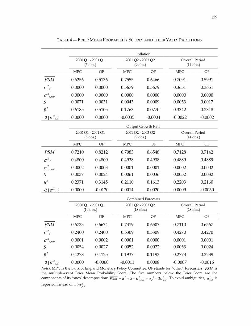
159

TABLE 4 ― BRIER MEAN PROBABILITY SCORES AND THEIR YATES PARTITIONS

Inflation

2000 Q1 - 2001 Q1

(5 obs.) 2001 Q2 - 2003 Q2 (9 obs.) Overall Period

(14 obs.)

MPC OF MPC OF MPC OF

PSM 0.6256 0.5136 0.7555 0.6466 0.7091 0.5991

σ

2d 0.0000 0.0000 0.5679 0.5679 0.3651 0.3651

σ

2p,min 0.0000 0.0000 0.0000 0.0000 0.0000 0.0000

S 0.0071 0.0031 0.0043 0.0009 0.0053 0.0017

B2 0.6185 0.5105 0.1763 0.0770 0.3342 0.2318

-2 [σ

2p,d] 0.0000 0.0000 -0.0035 -0.0004 -0.0022 -0.0002

Output Growth Rate

2000 Q1 - 2001 Q1 (5 obs.) 2001 Q2 - 2003 Q2

(9 obs.) Overall Period (14 obs.)

MPC OF MPC OF MPC OF

PSM 0.7210 0.8212 0.7083 0.6548 0.7128 0.7142

σ

2d 0.4800 0.4800 0.4938 0.4938 0.4889 0.4889

σ

2p,min 0.0002 0.0003 0.0001 0.0001 0.0002 0.0002

S 0.0037 0.0024 0.0061 0.0036 0.0052 0.0032

B2 0.2371 0.3145 0.2110 0.1613 0.2203 0.2160

-2 [σ

2p,d] 0.0000 -0.0120 0.0014 0.0020 0.0009 -0.0030

Combined Forecasts

2000 Q1 - 2001 Q1

(10 obs.) 2001 Q2 - 2003 Q2 (18 obs.) Overall Period

(28 obs.)

MPC OF MPC OF MPC OF

PSM 0.6733 0.6674 0.7319 0.6507 0.7110 0.6567

σ

2d 0.2400 0.2400 0.5309 0.5309 0.4270 0.4270

σ

2p,min 0.0001 0.0002 0.0001 0.0000 0.0001 0.0001

S 0.0054 0.0027 0.0052 0.0022 0.0053 0.0024

B2 0.4278 0.4125 0.1937 0.1192 0.2773 0.2239

-2 [σ

2p,d] 0.0000 -0.0060 -0.0011 0.0008 -0.0007 -0.0016

Notes: MPC is the Bank of England Monetary Policy Committee. OF stands for “other” forecasters. PSM is the multiple-event Brier Mean Probability Score. The five numbers below the Brier Score are the components of its Yates’ decomposition: 2

,22

min,2 2 dpdpSBPSM σσσ −+++= . To avoid ambiguities, 2

,dpσ is

reported instead of 2,2 dpσ−

160

TABLE 5 ― BRIER SCORES HYPOTHESES TESTS

Null: OFMPC PSMPSM =

CB-statistic p-value

Inflation Forecast 5.2502 0.0002

Output Growth Forecast 0.2737 0.7886 Notes: MPC is the Bank of England Monetary Policy Committee. OF stands for “other” forecasters. PSM is the multiple-event Brier Mean Probability Score. CB is the statistic developed in this paper, given by equation (35).

161

TABLE 6 ― DISINFLATION PERIODS AND SACRIFICE RATIOS

Episode

Initial Inflation

(π0)

Change in Inflation

(∆π)

Length of Disinflation

(LNG) (Quarters)

Speed of Disinflation

(SPD)

Sacrifice Ratio (SR)

Australia

1974:2-1978:1 14.60 6.57 15 0.4380 0.7234 1982:1-1984:1 10.50 4.98 8 0.6225 1.2782 1986:2-1993:1 * 8.99 7.83 27 0.2900 -0.4200 Canada

1974:2-1976:4 10.60 3.14 10 0.3140 0.6273 1981:2-1985:2 11.60 7.83 16 0.4894 2.3729 1990:1-1993:4 * 5.85 4.85 15 0.3233 2.6300 1996:1-1997:3 * 2.05 0.84 6 0.1400 0.7600 France

1974:2-1976:4 11.90 2.98 10 0.2980 0.9070 1981:1-1986:4 13 10.42 23 0.4530 0.5997 Germany

1965:4-1967:3 3.67 2.43 7 0.3471 2.5590 1973:1-1977:3 6.92 4.23 18 0.2350 2.6358 1980:1-1986:3 5.86 5.95 26 0.2288 3.5565 1992:2-1995:4 * 5.13 3.74 14 0.2671 0.7500 Italy

1963:3-1967:4 6.79 5.74 17 0.3376 2.6539 1977:1-1978:2 16.50 4.30 5 0.8600 0.9776 1980:1-1987:2 19.10 14.56 29 0.5021 1.5992 1989:4-1993:3 * 6.62 2.54 15 0.1693 -1.2800 1995:1-1996:3 * 4.72 1.86 6 0.3100 -0.5400 Japan

1962:3-1963:1 8.11 3.00 2 1.5000 0.5309 1965:1-1967:2 5.99 2.20 9 0.2444 1.6577

162

TABLE 6 ― CONTINUED

Episode

Initial Inflation

(π0)

Change in Inflation

(∆π)

Length of Disinflation

(LNG) (Quarters)

Speed of Disinflation

(SPD)

Sacrifice Ratio (SR)

Japan

1970:3-1971:2 7.53 2.09 3 0.6967 1.2689 1974:1-1978:3 17.10 13.21 18 0.7339 0.6068 1980:2-1983:4 6.68 5.07 14 0.3621 0.0174 1984:2-1987:1 2.29 2.11 11 0.1918 1.4801 1990:2-1996:1 * 3.74 3.85 23 0.1674 -0.8900 New Zealand

1985:4-1992:2 * 16.68 15.62 26 0.6008 -0.2300 Sweden

1977:1-1978:4 * 11.53 3.06 7 0.4371 1.4700 1980:3-1986:3 * 12.84 8.77 24 0.3654 1.6100 1990:1-1993:1 * 10.02 7.07 12 0.5892 -0.2100 1993:4-1997:3 * 3.49 3.56 11 0.3236 -1.0400 Switzerland

1973:4-1977:4 9.42 8.28 16 0.5175 1.8509 1981:3-1983:4 6.15 3.86 9 0.4289 1.2871 1990:4-1997:3 * 5.79 5.53 27 0.2048 1.4200 United Kingdom

1961:2-1963:3 4.24 2.10 9 0.2333 1.9105 1965:2-1966:3 4.91 2.69 5 0.5380 -0.0063 1975:1-1978:2 19.7 9.71 13 0.7469 0.8679 1980:2-1983:3 15.4 11.12 13 0.8554 0.2935 1984:2-1986:3 6.19 3.03 9 0.3367 0.8680 1989:2-1993:3 * 9.13 7.37 17 0.4335 1.1200 United States

1969:4-1971:4 5.67 2.14 8 0.2675 2.9364 1974:1-1976:4 9.70 4.00 11 0.3636 2.3914 1980:1-1983:4 12.10 8.83 15 0.5887 1.8320 1989:4-1994:3 * 5.28 2.65 19 0.1395 3.6800

* Episodes identified by the authors.

163

TABLE 7 ― DESCRIPTIVE STATISTICS OF SACRIFICE RATIOS AND CHARACTERIZATIONS

Averages

Decade

Number of Identified

Disinflation Episodes

Initial Inflation

(π0)

Change in Inflation

(∆π)

Length of Disinflation

(LNG) (Quarters)

Speed of Disinflation

(SPD)

Sacrifice Ratio (SR)

1960-1970 7 5.63 2.90 8 0.4954 1.7489 1970-1980 11 12.32 5.60 11 0.5128 1.3025 1980-1990 14 10.53 7.86 18 0.4511 1.1532 1990-2000 11 5.62 3.99 15 0.2789 0.5818 1960-2000 43 8.93 5.48 14 0.4301 1.1422

164

TABLE 8 ― TRADITIONAL FACTORS - CAUSAL STRUCTURE IMPOSED BY BALL (1994)

Speed of Disinflation (from Table 5.4, Ball)

Frequency of the Data Imposed Causality Structure and

Sign of Estimated Coefficient (in Parenthesis)

(1) Quarterly ( )SRSPD

−→

(2) Annual ( )SRSPD

−→

(3) Quarterly ( ) ( )LNGSR

+−←→∆π

(4) Annual ( ) ( )LNGSR

+−←→∆π

Initial Inflation (from Table 5.7)

Frequency of the Data Imposed Causality Structure and

Sign of Empirical Result

(1) Quarterly ( )SR

−→0π

(2) Quarterly

( )

( )

DUR

LNGSR−

+

↑←→

↓∆

0π

π

(3) Annual SR→0π

(4) Annual

( )

( )

DUR

LNGSR−

+

↑←→

↓∆

0π

π

Notes: SR denotes the sacrifice ratio, π0 is the inflation level at the beginning of the identified disinflation period, ∆π stands for the change of inflation during the disinflation period, LNG is the length of the disinflation episode, SPD stands for speed of disinflation, i.e. the quotient between the ∆π and LNG, the duration of contracts (taken from Bruno and Sachs, 1985) is denoted by DUR. The sign obtained by Ball’s regressions is between parentheses next to the edge. When there is no sign associated to an edge indicates that the estimated coefficient was not statistically significant at the 10% confidence level.

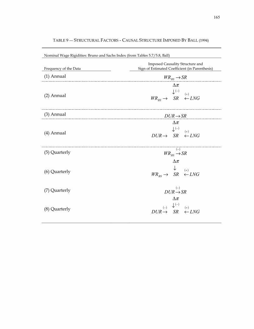
165

TABLE 9 ― STRUCTURAL FACTORS - CAUSAL STRUCTURE IMPOSED BY BALL (1994)

Nominal Wage Rigidities: Bruno and Sachs Index (from Tables 5.7/5.8, Ball)

Frequency of the Data Imposed Causality Structure and

Sign of Estimated Coefficient (in Parenthesis)

(1) Annual SRWRBS →

(2) Annual ( )

( )LNGSRWRBS

+−

←↓∆

→

π

(3) Annual SRDUR→

(4) Annual ( )

( )LNGSRDUR

+−

←↓∆

→

π

(5) Quarterly ( )

SRWRBS

−→

(6) Quarterly ( )LNGSRWRBS

+←

↓∆

→

π

(7) Quarterly ( )SRDUR

−→

(8) Quarterly ( )( )

( )LNGSRDUR

+−

−←

↓∆

→

π

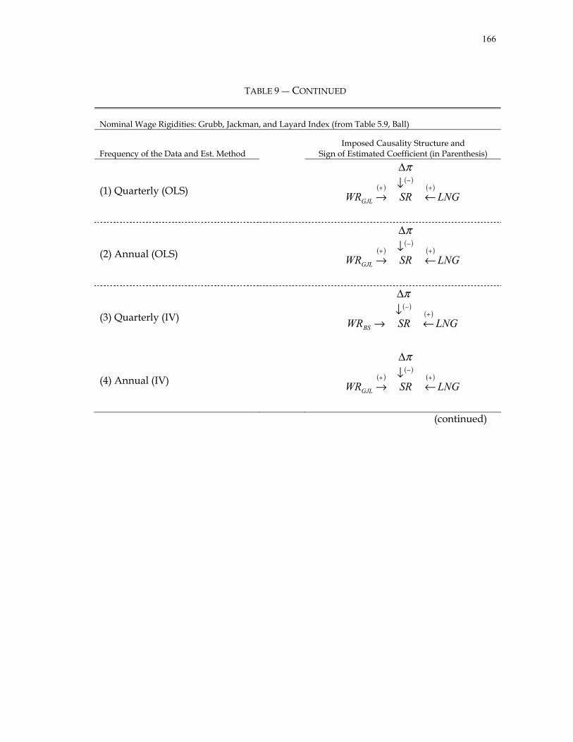
166

TABLE 9 ― CONTINUED

Nominal Wage Rigidities: Grubb, Jackman, and Layard Index (from Table 5.9, Ball)

Frequency of the Data and Est. Method Imposed Causality Structure and

Sign of Estimated Coefficient (in Parenthesis)

(1) Quarterly (OLS) ( )( )

( )LNGSRWRGJL

+−

+←

↓∆

→

π

(2) Annual (OLS) ( )( )

( )LNGSRWRGJL

+−

+←

↓∆

→

π

(3) Quarterly (IV) ( )

( )LNGSRWRBS

+−

←↓∆

→

π

(4) Annual (IV) ( )( )

( )LNGSRWRGJL

+−

+←

↓∆

→

π

(continued)

167

TABLE 9 ― CONTINUED

Openness (from Table 5.12, Ball)

Frequency of the Data Imposed Causality Structure and

Sign of Estimated Coefficient (in Parenthesis)

(1) Quarterly SROPN → (2) Annual SROPN →

(3) Quarterly

( )

( )

DUR

LNGSROPN↑

←→

↓∆

+

−

π

(4) Annual

( )

( )

DUR

LNGSROPN↑

←→

↓∆

+

−

π

Notes: SR denotes the sacrifice ratio, π0 is the inflation level at the beginning of the identified disinflation period, ∆π stands for the change of inflation during the disinflation period, LNG is the length of the disinflation episode, SPD stands for speed of disinflation, i.e. the quotient between the ∆π and LNG, the duration of contracts and the degree of wage responsiveness (taken from Bruno and Sachs, 1985) are denoted by DUR and WRBS. Grubb, Jackman, and Layard’s (1983) wage rigidity index is denoted by WRGJL. OPN is Romer’s openness index, i.e. the proportion of imports on the GDP. The sign obtained by Ball’s regressions is between parentheses next to the edge. When there is no sign associated to an edge indicates that the estimated coefficient was not statistically significant at the 10% confidence level.

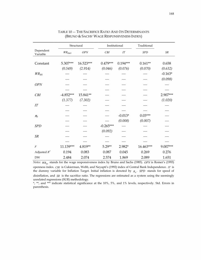
168

TABLE 10 ― THE SACRIFICE RATIO AND ITS DETERMINANTS (BRUNO & SACHS’ WAGE RESPONSIVENESS INDEX)

Structural Institutional Traditional Dependent Variable WRB&S OPN CBI IT SPD SR

Constant 5.307*** 16.523*** 0.479*** 0.194*** 0.161** 0.658 (0.549) (2.914) (0.046) (0.076) (0.070) (0.632) WRBS ---- ---- ---- ---- ---- -0.163* ---- ---- ---- ---- ---- (0.098) OPN ---- ---- ---- ---- ---- ----

---- ---- ---- ---- ---- ----

CBI -4.852*** 15.841** ---- ---- ---- 2.907*** (1.377) (7.302) ---- ---- ---- (1.020) IT ---- ---- ---- ---- ---- ----

---- ---- ---- ---- ---- ----

π0

---- ---- ---- -0.013* 0.03*** ----

---- ---- ---- (0.008) (0.007) ----

SPD ---- ---- -0.265*** ---- ---- ----

---- ---- (0.092) ---- ---- ----

SR ---- ---- ---- ---- ---- ----

---- ---- ---- ---- ---- ----

F 11.139*** 4.819** 5.29** 2.982* 16.463*** 9.007***Adjusted R2 0.194 0.083 0.087 0.045 0.269 0.276 DW 2.484 2.074 2.574 1.869 2.089 1.651

Notes: BSWR stands for the wage responsiveness index by Bruno and Sachs (1985). OPN is Romer’s (1993)

openness index. CBI is Cukierman, Webb, and Neyapti’s (1992) index of Central Bank Independence. IT is the dummy variable for Inflation Target. Initial inflation is denoted by

0π . SPD stands for speed of disinflation, and SR is the sacrifice ratio. The regressions are estimated as a system using the seemingly unrelated regressions (SUR) methodology. *, **, and *** indicate statistical significance at the 10%, 5%, and 1% levels, respectively. Std. Errors in parenthesis.

169

TABLE 11 ― THE SACRIFICE RATIO AND ITS DETERMINANTS (GRUBB, JACKMAN & LAYARD’S WAGE RIGIDITY INDEX)

Structural Institutional Traditional

Dependent Variable OPN CBI IT SPD SR

Constant 18.981*** 0.479*** 0.217*** 0.158** -0.369 (2.241) (0.046) (0.073) (0.070) (0.359) WRGJL -5.690*** ---- ---- ---- 0.383*** (0.969) ---- ---- ---- (0.155) OPN ---- ---- ---- ---- ---- ---- ---- ---- ---- ----

CBI 19.954*** ---- ---- ---- 3.409*** (5.555) ---- ---- ---- (0.891) IT ---- ---- ---- ---- ---- ---- ---- ---- ---- ----

π0 ---- ---- -0.016** 0.03*** ----

---- ---- (0.007) (0.007) ----

SPD ---- -0.264*** ---- ---- ---- ---- (0.092) ---- ---- ----

SR ---- ---- ---- ---- ---- ---- ---- ---- ---- ----

F 16.956*** 5.29** 2.982* 16.463*** 10.209***Adjusted R2 0.43 0.087 0.043 0.269 0.303 DW 2.525 2.574 1.906 2.085 1.734

Notes: GJLWR stands for the wage responsiveness index by Grubb, Jackman, and Layard (1983). OPN is

Romer’s (1993) openness index. CBI is Cukierman, Webb, and Neyapti’s (1992) index of Central Bank Independence. IT is the dummy variable for Inflation Target. Initial inflation is denoted by

0π . SPD stands for speed of disinflation, and SR is the sacrifice ratio. The regressions are estimated as a system using the seemingly unrelated regressions (SUR) methodology. *, **, and *** indicate statistical significance at the 10%, 5%, and 1% levels, respectively. Std. Errors in parenthesis.

170

TABLE 12 ― THE SACRIFICE RATIO AND THE SPEED OF DISINFLATION: THE FRONT DOOR PATH

Dependent Variable SR

(I) (II) (II) Constant -0.381 -0.364 1.189*** (0.381) (0.557) (0.368) WRGJL 0.337** 0.338** 0.422*** (0.166) (0.168) (0.188) CBI (The “blocking” variable) 3.53*** 3.515*** ----

(0.949) (1.023) ----

SPD ---- -0.028‡ -0.791‡‡ ---- (0.652) (0.691) F 10.209*** 6.637*** 3.188** Adjusted R2 0.305 0.287 0.094 DW 1.747 1.740 1.762

Notes: GJLWR stands for the wage responsiveness index by Grubb, Jackman, and Layard (1983). CBI is

Cukierman, Webb, and Neyapti’s (1992) index of Central Bank Independence. SPD stands for speed of disinflation, and SR is the sacrifice ratio. The regressions are estimated using OLS. *, **, and *** indicate statistical significance at the 10%, 5%, and 1% levels, respectively. Std. Errors in parenthesis. ‡ and ‡‡ indicate statistical significance at the 95%, and 25%, respectively.

171

APPENDIX B

FIGURES

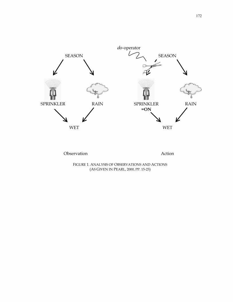
172

FIGURE 1. ANALYSIS OF OBSERVATIONS AND ACTIONS (AS GIVEN IN PEARL, 2000, PP. 15-23)

WET

RAIN SPRINKLER

SEASON

WET

RAIN SPRINKLER=ON

SEASON

Observation Action

do-operator

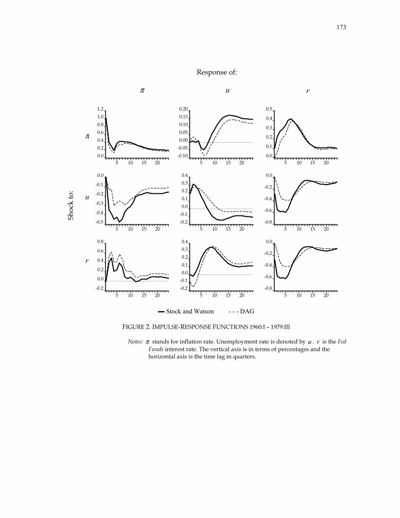
173

Response of:

π u r

π

u

Shoc

k to

:

r

0.00.20.40.60.81.01.2

5 10 15 20-0.10-0.050.000.050.100.150.20

5 10 15 200.0

0.1

0.2

0.3

0.4

0.5

5 10 15 20

-0.5

-0.4

-0.3

-0.2

-0.1

0.0

5 10 15 20-0.2-0.10.00.10.20.30.4

5 10 15 20-0.8

-0.6

-0.4

-0.2

0.0

5 10 15 20

-0.2

0.0

0.2

0.4

0.6

0.8

5 10 15 20-0.2-0.10.00.10.20.30.4

5 10 15 20-0.8

-0.6

-0.4

-0.2

0.0

5 10 15 20

▬ Stock and Watson - - - DAG

FIGURE 2. IMPULSE-RESPONSE FUNCTIONS 1960:I – 1979:III Notes: π stands for inflation rate. Unemployment rate is denoted by u . r is the Fed

Funds interest rate. The vertical axis is in terms of percentages and the horizontal axis is the time lag in quarters.

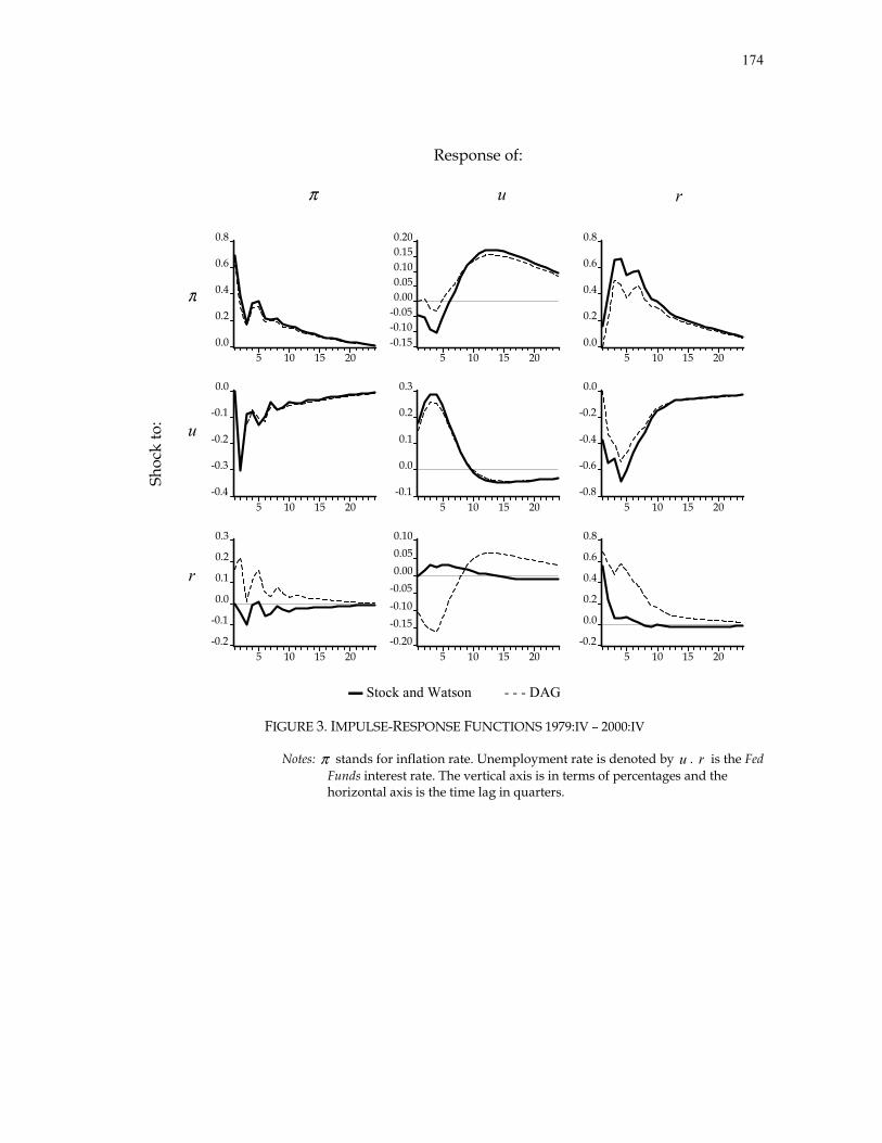
174

Response of:

π u r

π

u

Shoc

k to

:

r

0.0

0.2

0.4

0.6

0.8

5 10 15 20-0.15-0.10-0.050.000.050.100.150.20

5 10 15 200.0

0.2

0.4

0.6

0.8

5 10 15 20

-0.4

-0.3

-0.2

-0.1

0.0

5 10 15 20-0.1

0.0

0.1

0.2

0.3

5 10 15 20-0.8

-0.6

-0.4

-0.2

0.0

5 10 15 20

-0.2

-0.1

0.0

0.1

0.2

0.3

5 10 15 20-0.20-0.15-0.10-0.050.000.050.10

5 10 15 20-0.2

0.0

0.2

0.4

0.6

0.8

5 10 15 20

▬ Stock and Watson - - - DAG

FIGURE 3. IMPULSE-RESPONSE FUNCTIONS 1979:IV – 2000:IV Notes: π stands for inflation rate. Unemployment rate is denoted by u . r is the Fed

Funds interest rate. The vertical axis is in terms of percentages and the horizontal axis is the time lag in quarters.

175

FIGURE 4. MONETARY POLICY COMMITTEE FAN CHART OF INFLATION

Infla

tion

Time

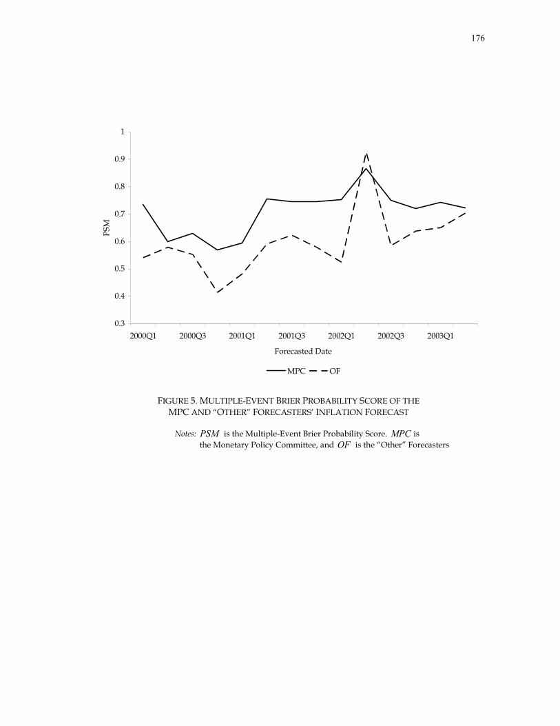
176

0.3

0.4

0.5

0.6

0.7

0.8

0.9

1

2000Q1 2000Q3 2001Q1 2001Q3 2002Q1 2002Q3 2003Q1

Forecasted Date

PSM

MPC OF

FIGURE 5. MULTIPLE-EVENT BRIER PROBABILITY SCORE OF THE MPC AND “OTHER” FORECASTERS’ INFLATION FORECAST

Notes: PSM is the Multiple-Event Brier Probability Score. MPC is

the Monetary Policy Committee, and OF is the “Other” Forecasters

177

0

0.2

0.4

0.6

0.8

1

2000Q1 2000Q3 2001Q1 2001Q3 2002Q1 2002Q3 2003Q1

Forecasted Date

PSM

MPC OF

FIGURE 6. MULTIPLE-EVENT BRIER PROBABILITY SCORE FOR THE MPC AND “OTHER” FORECASTERS’ REAL GDP GROWTH FORECAST

Notes: PSM is the Multiple-Event Brier Probability Score. MPC is

the Monetary Policy Committee, and OF is the “Other” Forecasters

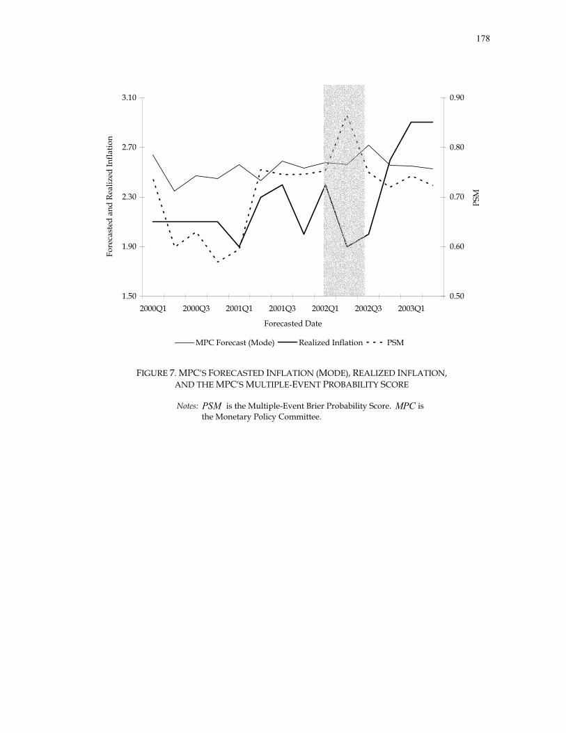
178

1.50

1.90

2.30

2.70

3.10

2000Q1 2000Q3 2001Q1 2001Q3 2002Q1 2002Q3 2003Q1

Forecasted Date

Fore

cast

ed a

nd R

ealiz

ed In

flatio

n

0.50

0.60

0.70

0.80

0.90

PSM

MPC Forecast (Mode) Realized Inflation PSM

FIGURE 7. MPC’S FORECASTED INFLATION (MODE), REALIZED INFLATION, AND THE MPC’S MULTIPLE-EVENT PROBABILITY SCORE Notes: PSM is the Multiple-Event Brier Probability Score. MPC is

the Monetary Policy Committee.

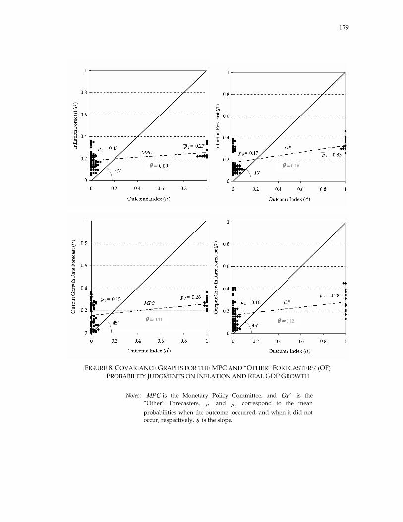
179

FIGURE 8. COVARIANCE GRAPHS FOR THE MPC AND “OTHER” FORECASTERS’ (OF)

PROBABILITY JUDGMENTS ON INFLATION AND REAL GDP GROWTH

Notes: MPC is the Monetary Policy Committee, and OF is the “Other” Forecasters.

1p and 0p correspond to the mean

probabilities when the outcome occurred, and when it did not occur, respectively. θ is the slope.

θθθθ

====

θθθθ

====

0.16

θθθθ

====

0.11 θθθθ

====

0.12

180

FIGURE 9. INFLATION (UPPER), OUTPUT, AND POTENTIAL (TREND) OUTPUT (LOWER) DURING DISINFLATION PERIODS. π DENOTES INFLATION, y IS OUTPUT, AND t IS TIME

181

FIGURE 10. THREE DIRECTED ACYCLICAL GRAPHS

X Y

Z

Causal Fork

X Y

Z

Inverted Causal Fork

(Collider)

X Y

Z

Causal Chain

182

FIGURE 11. PROCEDURE TO DIRECT EDGES INA DIRECTED ACYCLICAL GRAPH USING THE NOTION OF D-SEPARATION

X Y

Z

Causal Fork

X Y

Z

Inverted Causal Fork

(Collider)

X Y

Z

Causal Chain

ρρρρX,Y ≠ 0 ρρρρX,Z ≠ 0 ρρρρZ,Y ≠ 0 ρρρρX,Y│Z = 0 ρρρρX,Z│Y ≠ 0 ρρρρZ,Y│X ≠ 0

ρρρρX,Y ≠ 0 ρρρρX,Z = 0 ρρρρZ,Y ≠ 0 ρρρρX,Y│Z ≠ 0 ρρρρX,Z│Y ≠ 0 ρρρρZ,Y│X ≠ 0

ρρρρX,Y ≠ 0 ρρρρX,Z ≠ 0 ρρρρZ,Y ≠ 0 ρρρρX,Y│Z = 0 ρρρρX,Z│Y ≠ 0 ρρρρZ,Y│X ≠ 0

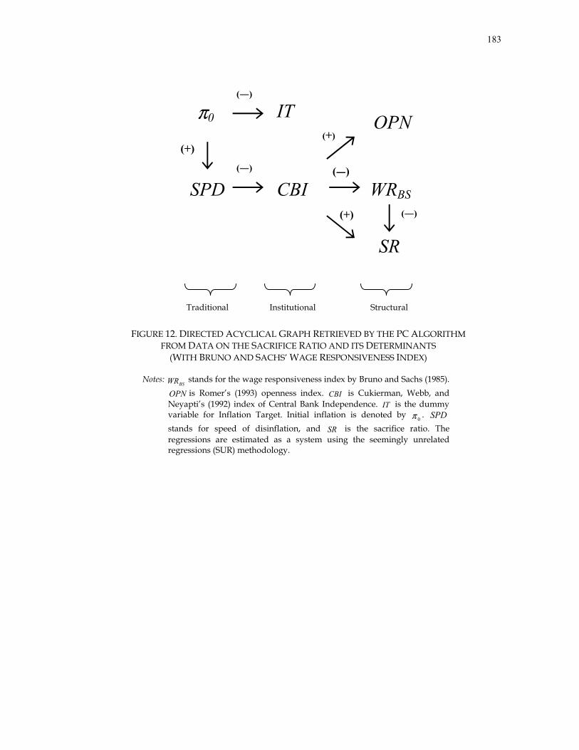
183

FIGURE 12. DIRECTED ACYCLICAL GRAPH RETRIEVED BY THE PC ALGORITHM FROM DATA ON THE SACRIFICE RATIO AND ITS DETERMINANTS

(WITH BRUNO AND SACHS’ WAGE RESPONSIVENESS INDEX)

Notes: BSWR stands for the wage responsiveness index by Bruno and Sachs (1985).

OPN is Romer’s (1993) openness index. CBI is Cukierman, Webb, and Neyapti’s (1992) index of Central Bank Independence. IT is the dummy variable for Inflation Target. Initial inflation is denoted by

0π . SPD stands for speed of disinflation, and SR is the sacrifice ratio. The regressions are estimated as a system using the seemingly unrelated regressions (SUR) methodology.

π0 IT

SPD

(―)

(+)

CBI(―) (―)

(+)

(+) OPN

WRBS

SR

Traditional Institutional Structural

(―)

184

FIGURE 13. DIRECTED ACYCLICAL GRAPH RETRIEVED BY THE PC ALGORITHM FROM DATA ON THE SACRIFICE RATIO AND ITS DETERMINANTS

(WITH GRUBB, JACKMAN, AND LAYARD’S WAGE RIGIDITY INDEX)

Notes: GJLWR stands for the wage responsiveness index by Grubb, Jackman, and

Layard (1983). OPN is Romer’s (1993) openness index. CBI is Cukierman, Webb, and Neyapti’s (1992) index of Central Bank Independence. IT is the dummy variable for Inflation Target. Initial inflation is denoted by

0π .

SPD stands for speed of disinflation, and SR is the sacrifice ratio. The regressions are estimated as a system using the seemingly unrelated regressions (SUR) methodology.

π0 IT

SPD

(―)

(+)

CBI(―)

(+)

(+) OPN

SR

Traditional Institutional Structural

WRGJL

(―)

(+)

185

APPENDIX C

PROGRAMS

186

SAMPLE PROGRAM STRUCTURAL VECTOR AUTOREGRESSIONS AND THE TAYLOR RULE *-----------------------------------------------------------*- RATS v5 Program for Structural Vector Autoregressions -*- and the Taylor Rule -*- By Gabriel Casillas -*- May 31st., 2004 (Version 1.0) -*- Last Update: June 10th, 2004 -*- WARNING: THIS IS JUST AN EXAMPLE FOR THE DAG -*- EMPIRICALLY-BASED CAUSAL STRUCTURES FOR THE -*- 1960:I-1979:III & 1979:IV-2000:IV PERIODS -*- USING STOCK AND WATSON's QUARTERLY DATA -*- ON INFLATION, UNEMPLOYMENT, AND INTEREST -*- RATES FOR THE US -*- -*-----------------------------------------------------------*-----------------------------------*- MAIN PROGRAM -*-----------------------------------************************************* INVOQUE PROCEDURES *************************************SOURCE C:\PROGRA~1\ESTIMA\WINRAT~1\BERNANKE.SRC************************************* LOAD DATA ************************************** -&-&-&-&-&-&-&-&-&-&-&-&-&-&-&-&-&* 1) Set starting year, starting period and* number of periods per year

CALENDAR 1955 1 4* 2) Set number and length of series

ALLOCATE 3 6* 3) Rename the series from numbers to actual names

EQV 1 TO 3P U R

* 4) Open Data SetOPEN DATA C:\A\TR\PUR.ASCDATA(FORMAT=FREE,ORG=OBS) 1955:1 2000:4 1 TO 3

* 5) Print the series to check that they are inside the* program* (This step is optional)

PRINT 1955:1 2000:4 1 TO 3* -&-&-&-&-&-&-&-&-&-&-&-&-&-&-&-&-&

************************************************** FISRT PERIOD ** SAMPLE 1: 1960:1 - 1979:3 STOCK AND WATSON **************************************************************************************************** DECLARE SYSTEM (4-LAG REDUCED-FORM VAR) **************************************************

SAMPLE P 1960:01 1979:03 P2SAMPLE U 1960:01 1979:03 U2

187

SAMPLE R 1960:01 1979:03 R2SYSTEM 4 to 6EQUATION 4 P2# CONSTANT P2{1 to 4} U2{1 to 4} R2{1 to 4}EQUATION 5 U2# CONSTANT P2{1 to 4} U2{1 to 4} R2{1 to 4}EQUATION 6 R2# CONSTANT P2{1 to 4} U2{1 to 4} R2{1 to 4}END(SYSTEM)

************************************************** INNOVATION ACCOUNTING **************************************************

DECLARE SYMMETRIC V42ESTIMATE(outsigma=v42) 1960:01 1979:03COMPUTE nreg4=%nregCOMPUTE nobs4=%nobs* Choleski DecompositionWRITE V42DECLARE rect pattern(3,3)INPUT pattern1 0 01 1 10 0 1* We need to let the BERNANKE Procedure in RATS* know which are the parameters in the K-Matrix* that have to be estimated. In this case they* are the elements (2,1) and (2,3)NONLIN A221 A223* Starting valuesCOMPUTE A221=-0.1, A223=-0.1* Continue CholeskiCOMPUTE A2=%identity(3)FIND min -2*log(%det(A2))+%sum(%log(%mqformdiag(V42,tr(A2)))) {COMPUTE A2(2,1)=A221, A2(2,3)=A223}END FINDWRITE 'MATRIX A2: ' A2@BERNANKE(Initial=A2,TEST,PRINT) V42 PATTERN FACTOR* ERRORS runs the Forecast Error Variance Decomposition* and the Impulse-Response Functions for the three equations* for 24-steps aheadERRORS(DECOMP=FACTOR,IMPULSES) 3 24# 4# 5# 6

************************************************** SAMPLE 2: 1979:4 - 2000:4 STOCK AND WATSON ** DECLARE SYSTEM (4-LAG REDUCED-FORM VAR) **************************************************

SAMPLE P 1979:04 2000:04 P3SAMPLE U 1979:04 2000:04 U3SAMPLE R 1979:04 2000:04 R3SYSTEM 7 to 9EQUATION 7 P3

188

# CONSTANT P3{1 to 4} U3{1 to 4} R3{1 to 4}EQUATION 8 U3# CONSTANT P3{1 to 4} U3{1 to 4} R3{1 to 4}EQUATION 9 R3# CONSTANT P3{1 to 4} U3{1 to 4} R3{1 to 4}END(SYSTEM)

************************************************** INNOVATION ACCOUNTING **************************************************

DECLARE SYMMETRIC V43ESTIMATE(outsigma=v43) 1979:04 2000:04COMPUTE nreg4=%nregCOMPUTE nobs4=%nobs* Choleski DecompositionWRITE V43DECLARE rect pattern(3,3)INPUT pattern1 0 10 1 10 0 1* We need to let the BERNANKE Procedure in RATS* know which are the parameters in the K-Matrix* that have to be estimated. In this case they* are the elements (1,3) and (2,3)NONLIN A313 A323* Starting valuesCOMPUTE A313=-0.1, A323=-0.1* Continue CholeskiCOMPUTE A3=%identity(3)FIND min -2*log(%det(A3))+%sum(%log(%mqformdiag(V42,tr(A3)))) {COMPUTE A3(1,3)=A313, A3(2,3)=A323}END FINDWRITE 'MATRIX A3: ' A3@BERNANKE(Initial=A3,TEST,PRINT) V43 PATTERN FACTOR* ERRORS runs the Forecast Error Variance Decomposition* and the Impulse-Response Functions for the three equations* for 24-steps aheadERRORS(DECOMP=FACTOR,IMPULSES) 3 24# 7# 8# 9

**************************************************************************************************

************************************************** PROGRAM END **************************************************WRITE ' 'WRITE ' -------------- 'WRITE ' END OF PROGRAM 'WRITE ' -------------- 'WRITE ' '

END

189

SAMPLE PROGRAMPROBABILITY FORECASTING AND CENTRAL BANK ACCOUNTABILITY

*-----------------------------------------------------------*- RATS v5 Program for Probability Forecasting Evaluation -*- By Gabriel Casillas & David A. Bessler -*- Sept. 30th., 2003 (Version 1.0) -*- March 26th., 2004 (Version 2.0) -*- Last Update: March 26th., 2004 & May 24th, 2004 -*- Version 2.0 -*- In just 10 steps you will have a Brier Probability -*- Score calculation and its Yates Covariance -*- Decomposition. -*- WARNING: THIS IS JUST AN EXAMPLE FOR THE BANK OF -*- BANK OF ENGLAND's MONETARY POLICY COMMITTEE -*- TWO YEARS-AHEAD INFLATION PROBABILITY -*- FORECASTS FOR THE PERIOD BETWEEN THE FIRST -*- QUARTER OF 2000 AND THE FIRST QUARTER OF -*- 2001. -*- NOTE: THE PROCEDURE IS AT THE BEGINING OF THE SAMPLE -*- PROGAM OUTPUT, AT THE END OF THIS PROGRAM -*-----------------------------------------------------------*-----------------------------------*- MAIN PROGRAM -*-----------------------------------************************************* INVOQUE PROCEDURES *************************************SOURCE C:\PRBBRIER\PROCS2.SRC

************************************* IMPORT DATA ************************************** -&-&-&-&-&-&-&-&-&-&-&-&-&-&-&-&-&* 1) Set starting year, starting period and* number of periods per year

CALENDAR 2000 1 4* 2) Set number and length of series

ALLOCATE 36 14* 3) Rename the series from numbers to actual names

EQV 1 TO 36PBFC1 PBFC2 PBFC3 PBFC4 PBFC5 PBFC6POFC1 POFC2 POFC3 POFC4 POFC5 POFC6PRC1 PRC2 PRC3 PRC4 PRC5 PRC6GBFC1 GBFC2 GBFC3 GBFC4 GBFC5 GBFC6GOFC1 GOFC2 GOFC3 GOFC4 GOFC5 GOFC6GRC1 GRC2 GRC3 GRC4 GRC5 GRC6

* 4) Open Data SetOPEN DATA c:\PRBBRIER\DATASET.TXTDATA(FORMAT=FREE,ORG=OBS) 2000:1 2003:2 1 TO 36

* 5) Print the series to check that they are inside the program* (This step is optional)

PRINT 2000:1 2003:2 1 TO 36* -&-&-&-&-&-&-&-&-&-&-&-&-&-&-&-&-&

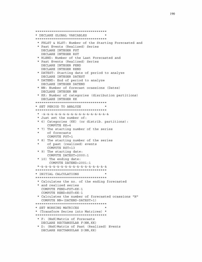
190

************************************* DECLARE GLOBAL VARIABLES ************************************** FRLST & RLST: Number of the Starting Forecasted and* Past Events (Realized) Series

DECLARE INTEGER FSTDECLARE INTEGER RST

* RLEND: Number of the Last Forecasted and* Past Events (Realized) Series

DECLARE INTEGER FENDDECLARE INTEGER REND

* DATEST: Starting date of period to analyzeDECLARE INTEGER DATEST

* DATEND: End of period to analyzeDECLARE INTEGER DATEND

* NN: Number of forecast ocassions (Dates)DECLARE INTEGER NN

* KK: Number of categories (disribution partitions)DECLARE INTEGER KK

************************************* SET PERIOD TO ANALYZE ************************************** -&-&-&-&-&-&-&-&-&-&-&-&-&-&-&-&-&* Just set the number of:* 6) Categories (KK) (or distrib. partitions):

COMPUTE KK=4* 7) The starting number of the series* of forecasts

COMPUTE FST=1* 8) The starting number of the series* of past (realized) events

COMPUTE RST=13* 9) The starting date:

COMPUTE DATEST=2000:1* 10) The ending date:

COMPUTE DATEND=2001:1*-&-&-&-&-&-&-&-&-&-&-&-&-&-&-&-&-&

************************************* INITIAL CALCULATIONS ************************************** Calculates the no. of the ending forecasted* and realized series

COMPUTE FEND=FST+KK-1COMPUTE REND=RST+KK-1

* Calculates the number of forecasted ocassions "N"COMPUTE NN=(DATEND-DATEST+1)

************************************* SET WORKING MATRICES ** (Transform Series into Matrices) ************************************** F: (NxK)Matrix of Forecasts

DECLARE RECTANGULAR F(NN,KK)* D: (NxK)Matrix of Past (Realized) Events

DECLARE RECTANGULAR D(NN,KK)

191

* Call procedure to transform series into matricesEXECUTE SMATRIX FST FEND NN KK DATEST DATENDCOMPUTE F=GGEXECUTE SMATRIX RST REND NN KK DATEST DATENDCOMPUTE D=GG

************************************* CALCULATE THE BRIER SCORE AND ** THE YATES PARTITION ************************************************************************** N1, DUPBR & VARD *************************************EXECUTE N1 RST REND NN KK DATEST DATEND* NN1: (Kx1)Vector of vertical sum of columns of D matrix

DECLARE RECTANGULAR NN1(KK,1)COMPUTE NN1=HH

* DUPBR: (Kx1)Vector 1/N x NN1DECLARE RECTANGULAR DUPBR(KK,1)COMPUTE DUPBR=JJ

* VARD: (Kx1)Vector of Var(d)DECLARE RECTANGULAR VARD(KK,1)COMPUTE VARD=QQ

************************************* FUPBAR & VARF *************************************EXECUTE FUPBAR FST FEND NN KK DATEST DATEND* FUPBR: (Kx1)Vector of vertical sum of columns of F matrix* multiplied by (1/N)

DECLARE RECTANGULAR FUPBR(KK,1)COMPUTE FUPBR=LLDECLARE RECTANGULAR VARF(KK,1)COMPUTE VARF=ZZ* The following thing is to have a numerical* value of (1/N) with no variable-type problemDECLARE REAL OONCOMPUTE OON=ONENDECLARE REAL OKKCOMPUTE OKK=OKEN

************************************* BIAS ************************************** BIAS: (Kx1)Vector of FUPBR-DUPBR

DECLARE RECTANGULAR BIAS(KK,1)COMPUTE BIAS=(FUPBR-DUPBR)

* We want Average Bias as wellDECLARE REAL SUMBIASCOMPUTE SUMBIAS=%SUM(BIAS)DECLARE REAL AVGBIASCOMPUTE AVGBIAS=OKK*SUMBIAS

* We also need BIAS^2, therefore:DECLARE RECTANGULAR BIAS2(KK,1)DO CONT=1,KK

COMPUTE BIAS2(CONT,1)=BIAS(CONT,1)**2END DO

192

************************************* N0 ************************************** NN0: (Kx1)Vector of N-N1

DECLARE RECTANGULAR NN0(KK,1)DO CONT=1,KKCOMPUTE NN0(CONT,1)=NN-NN1(CONT,1)

END DO************************************* F1UPBR *************************************DECLARE REAL ADDFDECLARE RECTANGULAR F1UPBR(KK,1)COMPUTE ADDF=0DO CONT2=1,KKDO CONT=1,NNIF D(CONT,CONT2)==1 {COMPUTE ADDF=ADDF+F(CONT,CONT2)}

END IFEND DOIF NN1(CONT2,1)==0 {COMPUTE F1UPBR(CONT2,1)=0}

END IFIF NN1(CONT2,1)<>0 {COMPUTE F1UPBR(CONT2,1)=ADDF*(1/NN1(CONT2,1))}

END IF* Clear the value of the accumulator ADDFCOMPUTE ADDF=0

END DO************************************* F0UPBR *************************************DECLARE RECTANGULAR F0UPBR(KK,1)COMPUTE ADDF=0DO CONT2=1,KKDO CONT=1,NNIF D(CONT,CONT2)==0 {COMPUTE ADDF=ADDF+F(CONT,CONT2)}

END IFEND DOIF NN0(CONT2,1)==0 {COMPUTE F0UPBR(CONT2,1)=0}

END IFIF NN0(CONT2,1)<>0 {COMPUTE F0UPBR(CONT2,1)=ADDF*(1/NN0(CONT2,1))}

END IF* Clear the value of the accumulator ADDF

COMPUTE ADDF=0END DO

************************************* VARF1 *************************************DECLARE RECTANGULAR VARF1(KK,1)COMPUTE ADDF=0

193

DO CONT2=1,KKIF NN1(CONT2,1)<>0 {DO CONT=1,NNIF D(CONT,CONT2)==1 {COMPUTE ADDF=ADDF+(F(CONT,CONT2)-F1UPBR(CONT2,1))**2}

END IFIF D(CONT,CONT2)==0 {COMPUTE ADDF=ADDF}

END IFEND DOCOMPUTE VARF1(CONT2,1)=(1/NN1(CONT2,1))*ADDF}

END IFIF NN1(CONT2,1)==0 {COMPUTE VARF1(CONT2,1)=0}

END IFCOMPUTE ADDF=0

END DO************************************* VARF0 *************************************DECLARE RECTANGULAR VARF0(KK,1)COMPUTE ADDF=0DO CONT2=1,KKIF NN0(CONT2,1)<>0 {DO CONT=1,NNIF D(CONT,CONT2)==0 {COMPUTE ADDF=ADDF+(F(CONT,CONT2)-F0UPBR(CONT2,1))**2}

END IFIF D(CONT,CONT2)==1 {COMPUTE ADDF=ADDF}

END IFEND DOCOMPUTE VARF0(CONT2,1)=(1/NN0(CONT2,1))*ADDF}

END IFIF NN0(CONT2,1)==0 {COMPUTE VARF0(CONT2,1)=0}

END IFCOMPUTE ADDF=0

END DO************************************* SCAT *************************************DECLARE RECTANGULAR SCAT(KK,1)DO CONT=1,KKCOMPUTE

SCAT(CONT,1)=(OON)*((NN1(CONT,1)*VARF1(CONT,1))+(NN0(CONT,1)*VARF0(CONT,1)))

END DO************************************* MINVAR *************************************DECLARE RECTANGULAR MINVAR(KK,1)DO CONT=1,KKCOMPUTE MINVAR(CONT,1)=VARF(CONT,1)-SCAT(CONT,1)

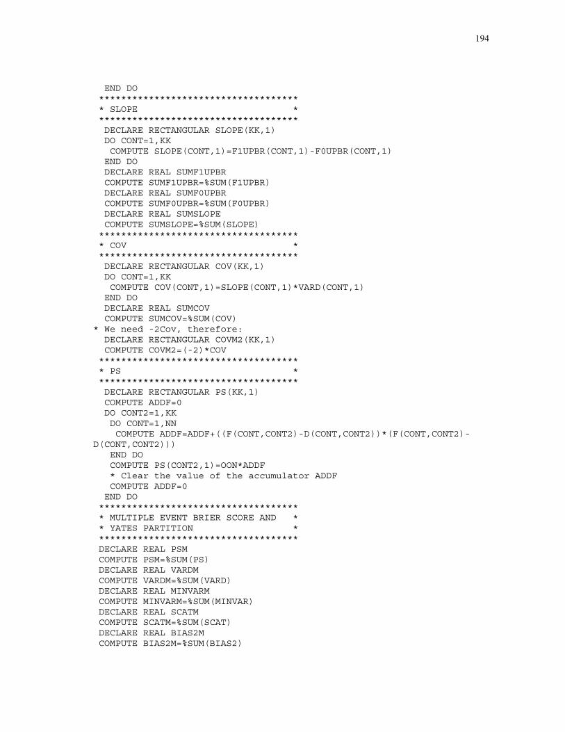
194

END DO************************************* SLOPE *************************************DECLARE RECTANGULAR SLOPE(KK,1)DO CONT=1,KKCOMPUTE SLOPE(CONT,1)=F1UPBR(CONT,1)-F0UPBR(CONT,1)

END DODECLARE REAL SUMF1UPBRCOMPUTE SUMF1UPBR=%SUM(F1UPBR)DECLARE REAL SUMF0UPBRCOMPUTE SUMF0UPBR=%SUM(F0UPBR)DECLARE REAL SUMSLOPECOMPUTE SUMSLOPE=%SUM(SLOPE)

************************************* COV *************************************DECLARE RECTANGULAR COV(KK,1)DO CONT=1,KKCOMPUTE COV(CONT,1)=SLOPE(CONT,1)*VARD(CONT,1)

END DODECLARE REAL SUMCOVCOMPUTE SUMCOV=%SUM(COV)

* We need -2Cov, therefore:DECLARE RECTANGULAR COVM2(KK,1)COMPUTE COVM2=(-2)*COV

************************************* PS *************************************DECLARE RECTANGULAR PS(KK,1)COMPUTE ADDF=0DO CONT2=1,KKDO CONT=1,NNCOMPUTE ADDF=ADDF+((F(CONT,CONT2)-D(CONT,CONT2))*(F(CONT,CONT2)-

D(CONT,CONT2)))END DOCOMPUTE PS(CONT2,1)=OON*ADDF* Clear the value of the accumulator ADDFCOMPUTE ADDF=0

END DO************************************* MULTIPLE EVENT BRIER SCORE AND ** YATES PARTITION *************************************DECLARE REAL PSMCOMPUTE PSM=%SUM(PS)DECLARE REAL VARDMCOMPUTE VARDM=%SUM(VARD)DECLARE REAL MINVARMCOMPUTE MINVARM=%SUM(MINVAR)DECLARE REAL SCATMCOMPUTE SCATM=%SUM(SCAT)DECLARE REAL BIAS2MCOMPUTE BIAS2M=%SUM(BIAS2)

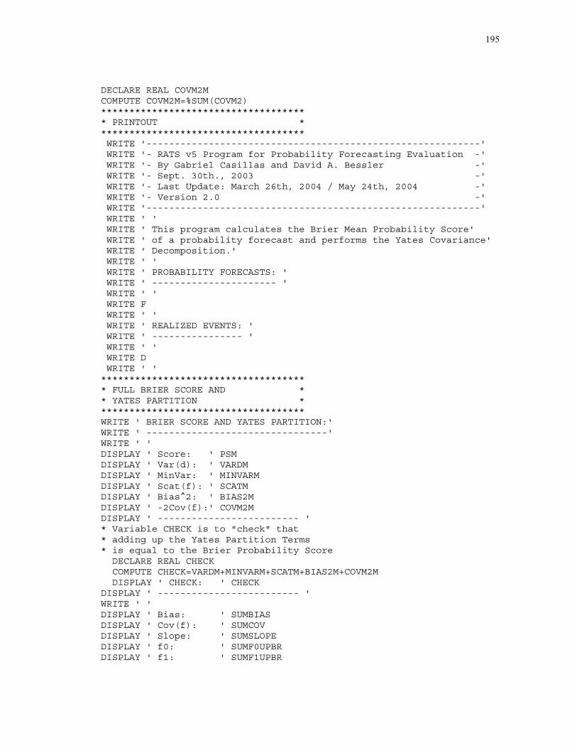
195

DECLARE REAL COVM2MCOMPUTE COVM2M=%SUM(COVM2)************************************* PRINTOUT *************************************WRITE '-----------------------------------------------------------'WRITE '- RATS v5 Program for Probability Forecasting Evaluation -'WRITE '- By Gabriel Casillas and David A. Bessler -'WRITE '- Sept. 30th., 2003 -'WRITE '- Last Update: March 26th, 2004 / May 24th, 2004 -'WRITE '- Version 2.0 -'WRITE '-----------------------------------------------------------'WRITE ' 'WRITE ' This program calculates the Brier Mean Probability Score'WRITE ' of a probability forecast and performs the Yates Covariance'WRITE ' Decomposition.'WRITE ' 'WRITE ' PROBABILITY FORECASTS: 'WRITE ' ---------------------- 'WRITE ' 'WRITE FWRITE ' 'WRITE ' REALIZED EVENTS: 'WRITE ' ---------------- 'WRITE ' 'WRITE DWRITE ' '

************************************* FULL BRIER SCORE AND ** YATES PARTITION *************************************WRITE ' BRIER SCORE AND YATES PARTITION:'WRITE ' --------------------------------'WRITE ' 'DISPLAY ' Score: ' PSMDISPLAY ' Var(d): ' VARDMDISPLAY ' MinVar: ' MINVARMDISPLAY ' Scat(f): ' SCATMDISPLAY ' Bias^2: ' BIAS2MDISPLAY ' -2Cov(f):' COVM2MDISPLAY ' ------------------------- '* Variable CHECK is to "check" that* adding up the Yates Partition Terms* is equal to the Brier Probability Score

DECLARE REAL CHECKCOMPUTE CHECK=VARDM+MINVARM+SCATM+BIAS2M+COVM2MDISPLAY ' CHECK: ' CHECK

DISPLAY ' ------------------------- 'WRITE ' 'DISPLAY ' Bias: ' SUMBIASDISPLAY ' Cov(f): ' SUMCOVDISPLAY ' Slope: ' SUMSLOPEDISPLAY ' f0: ' SUMF0UPBRDISPLAY ' f1: ' SUMF1UPBR

196

DISPLAY ' Average f: ' FUPBRDISPLAY ' Average d: ' DUPBRWRITE ' 'WRITE ' 'WRITE ' 'WRITE ' 'WRITE ' -------------- 'WRITE ' END OF PROGRAM 'WRITE ' -------------- 'WRITE ' '

END

197

SAMPLE OUTPUT PROBABILITY FORECASTING AND CENTRAL BANK ACCOUNTABILITY

*-----------------------------------*- PROCEDURE SMATRIX -*-----------------------------------PROCEDURE SMATRIX AA BB CC DD EE FF(01.0028) DECLARE RECTANGULAR GG(01.0028) DIM GG(CC,DD)(01.0051) MAKE GG EE FF(01.0084) # AA TO BB(01.0116) END PROCEDURE

*-----------------------------------*- PROCEDURE N1, DUPBAR & VARD -*-----------------------------------PROCEDURE N1 AA BB CC DD EE FF(01.0028) DECLARE RECTANGULAR GG(01.0028) DECLARE RECTANGULAR WW(01.0028) DECLARE RECTANGULAR HH(01.0028) DECLARE RECTANGULAR JJ(01.0028) DECLARE RECTANGULAR QQ(01.0028) DECLARE REAL ONEN1(01.0028) DECLARE REAL ONEN(01.0028) DECLARE RECTANGULAR AKK(01.0028) DECLARE REAL OKEN1(01.0028) DECLARE REAL OKEN(01.0028) DIM GG(CC,DD) WW(CC,1) HH(DD,1) JJ(DD,1) QQ(DD,1) AKK(DD,1)(01.0136) MAKE GG EE FF(01.0169) # AA TO BB(01.0201) * N1 REALLY STARTS HERE(01.0201) DO CONT=1,DD(02.0233) COMPUTE WW=%XCOL(GG,CONT)(02.0258) COMPUTE HH(CONT,1)=%SUM(WW)(02.0285) END DO CONT(01.0287) * DUPBAR STARTS HERE(01.0287) * By the way, I had to use ONEN1 and ONEN as artificial(01.0287) * variables to transform the type that emerged from %ROWS(01.0287) COMPUTE ONEN1=%ROWS(WW)(01.0309) COMPUTE ONEN=(1/ONEN1)(01.0333) COMPUTE JJ=ONEN*HH(01.0358) * By the way, I had to use OKEN1 and OKEN as artificial(01.0358) * variables to transform the type that emerged from %ROWS(01.0358) COMPUTE OKEN1=%ROWS(HH)(01.0380) COMPUTE OKEN=(1/OKEN1)(01.0404) COMPUTE AKK=OKEN*HH(01.0429) * VARD STARTS HERE(01.0429) DO CONT=1,DD(02.0461) COMPUTE QQ(CONT,1)=JJ(CONT,1)*(1-(JJ(CONT,1)))(02.0515) END DO CONT(01.0517) END PROCEDURE

*-----------------------------------

198

*- PROCEDURE FUPBAR & VARF -*-----------------------------------PROCEDURE FUPBAR AA BB CC DD EE FF(01.0028) DECLARE RECTANGULAR GG(01.0028) DECLARE RECTANGULAR WW(01.0028) DECLARE RECTANGULAR HH(01.0028) DECLARE RECTANGULAR LL(01.0028) DECLARE RECTANGULAR ZZ(01.0028) DECLARE REAL ONEN1(01.0028) DECLARE REAL ONEN(01.0028) DECLARE REAL SUMA(01.0028) DIM GG(CC,DD) WW(CC,1) HH(DD,1) JJ(DD,1) ZZ(DD,1)(01.0119) MAKE GG EE FF(01.0152) # AA TO BB(01.0184) * FUPBAR REALLY STARTS HERE(01.0184) DO CONT=1,DD(02.0216) COMPUTE WW=%XCOL(GG,CONT)(02.0241) COMPUTE HH(CONT,1)=%SUM(WW)(02.0268) END DO CONT(01.0270) COMPUTE ONEN1=%ROWS(WW)(01.0292) COMPUTE ONEN=(1/ONEN1)(01.0316) COMPUTE LL=ONEN*HH(01.0341) * VARF STARTS HERE(01.0341) * This is extremely important since the(01.0341) * calculation of Var(d) differs from the calculation(01.0341) * of Var(f)(01.0341) * Var(f) is calculated by the "usual variance formula"(01.0341) * multiplied by (N-1)/N. In other words, using the(01.0341) * population variance formula(01.0341) COMPUTE SUMA=0(01.0356) DO CONT2=1,DD(02.0388) DO CONT=1,CC(03.0420) COMPUTE SUMA=SUMA+(GG(CONT,CONT2)-LL(CONT2,1))**2(03.0478) END DO CONT(02.0480) COMPUTE ZZ(CONT2,1)=SUMA*(1/ONEN1)(02.0520) COMPUTE SUMA=0(02.0535) END DO CONT2(01.0537) END PROCEDURE

199

ENTRY PBFC1 PBFC2 PBFC3 PBFC42000:01 0.07 0.28 0.35 0.302000:02 0.13 0.34 0.32 0.212000:03 0.10 0.33 0.35 0.222000:04 0.19 0.36 0.33 0.122001:01 0.16 0.35 0.36 0.132001:02 0.10 0.15 0.21 0.212001:03 0.07 0.14 0.22 0.242001:04 0.17 0.18 0.22 0.232002:01 0.05 0.12 0.22 0.252002:02 0.10 0.16 0.23 0.242002:03 0.07 0.13 0.22 0.262002:04 0.10 0.15 0.22 0.232003:01 0.18 0.17 0.22 0.222003:02 0.14 0.17 0.23 0.23

ENTRY PBFC5 PBFC6 POFC1 POFC22000:01 0.00 0.00 0.11 0.392000:02 0.00 0.00 0.10 0.372000:03 0.00 0.00 0.13 0.382000:04 0.00 0.00 0.15 0.462001:01 0.00 0.00 0.16 0.412001:02 0.16 0.17 0.08 0.152001:03 0.18 0.15 0.07 0.122001:04 0.14 0.06 0.06 0.162002:01 0.19 0.17 0.07 0.152002:02 0.17 0.10 0.08 0.152002:03 0.20 0.11 0.08 0.142002:04 0.17 0.13 0.07 0.142003:01 0.14 0.07 0.06 0.152003:02 0.15 0.08 0.08 0.17

ENTRY POFC3 POFC4 POFC5 POFC62000:01 0.37 0.14 0.00 0.002000:02 0.39 0.14 0.00 0.002000:03 0.37 0.12 0.00 0.002000:04 0.30 0.10 0.00 0.002001:01 0.31 0.11 0.00 0.002001:02 0.32 0.29 0.11 0.062001:03 0.30 0.30 0.13 0.082001:04 0.33 0.29 0.12 0.052002:01 0.36 0.27 0.11 0.052002:02 0.32 0.28 0.11 0.062002:03 0.32 0.28 0.12 0.062002:04 0.33 0.30 0.11 0.052003:01 0.35 0.30 0.10 0.042003:02 0.32 0.26 0.12 0.06

ENTRY PRC1 PRC2 PRC3 PRC42000:01 0 1 0 02000:02 0 1 0 0

200

2000:03 0 1 0 02000:04 0 1 0 02001:01 0 1 0 02001:02 0 0 1 02001:03 0 0 1 02001:04 0 0 1 02002:01 0 0 1 02002:02 0 1 0 02002:03 0 0 1 02002:04 0 0 0 12003:01 0 0 0 12003:02 0 0 0 1

ENTRY PRC5 PRC6 GBFC1 GBFC22000:01 0 0 0.00 0.002000:02 0 0 0.04 0.092000:03 0 0 0.07 0.132000:04 0 0 0.07 0.132001:01 0 0 0.03 0.082001:02 0 0 0.00 0.042001:03 0 0 0.01 0.062001:04 0 0 0.01 0.072002:01 0 0 0.02 0.102002:02 0 0 0.02 0.092002:03 0 0 0.01 0.072002:04 0 0 0.02 0.102003:01 0 0 0.03 0.092003:02 0 0 0.01 0.08

ENTRY GBFC3 GBFC4 GBFC5 GBFC62000:01 0.00 0.00 0.00 0.002000:02 0.19 0.25 0.21 0.222000:03 0.22 0.26 0.20 0.122000:04 0.23 0.27 0.20 0.102001:01 0.19 0.28 0.25 0.172001:02 0.14 0.29 0.30 0.232001:03 0.18 0.31 0.29 0.152001:04 0.19 0.32 0.27 0.142002:01 0.27 0.36 0.20 0.052002:02 0.24 0.35 0.24 0.062002:03 0.22 0.36 0.27 0.082002:04 0.25 0.33 0.22 0.082003:01 0.21 0.31 0.26 0.102003:02 0.24 0.34 0.23 0.09

ENTRY GOFC1 GOFC2 GOFC3 GOFC42000:01 0.05 0.11 0.30 0.362000:02 0.05 0.15 0.28 0.342000:03 0.06 0.13 0.29 0.352000:04 0.07 0.17 0.28 0.312001:01 0.05 0.11 0.22 0.34

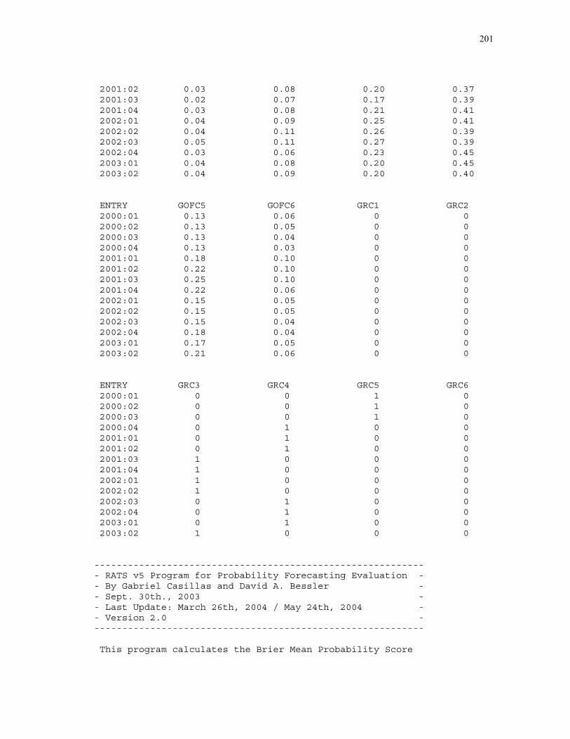
201

2001:02 0.03 0.08 0.20 0.372001:03 0.02 0.07 0.17 0.392001:04 0.03 0.08 0.21 0.412002:01 0.04 0.09 0.25 0.412002:02 0.04 0.11 0.26 0.392002:03 0.05 0.11 0.27 0.392002:04 0.03 0.06 0.23 0.452003:01 0.04 0.08 0.20 0.452003:02 0.04 0.09 0.20 0.40

ENTRY GOFC5 GOFC6 GRC1 GRC22000:01 0.13 0.06 0 02000:02 0.13 0.05 0 02000:03 0.13 0.04 0 02000:04 0.13 0.03 0 02001:01 0.18 0.10 0 02001:02 0.22 0.10 0 02001:03 0.25 0.10 0 02001:04 0.22 0.06 0 02002:01 0.15 0.05 0 02002:02 0.15 0.05 0 02002:03 0.15 0.04 0 02002:04 0.18 0.04 0 02003:01 0.17 0.05 0 02003:02 0.21 0.06 0 0

ENTRY GRC3 GRC4 GRC5 GRC62000:01 0 0 1 02000:02 0 0 1 02000:03 0 0 1 02000:04 0 1 0 02001:01 0 1 0 02001:02 0 1 0 02001:03 1 0 0 02001:04 1 0 0 02002:01 1 0 0 02002:02 1 0 0 02002:03 0 1 0 02002:04 0 1 0 02003:01 0 1 0 02003:02 1 0 0 0

------------------------------------------------------------ RATS v5 Program for Probability Forecasting Evaluation -- By Gabriel Casillas and David A. Bessler -- Sept. 30th., 2003 -- Last Update: March 26th, 2004 / May 24th, 2004 -- Version 2.0 ------------------------------------------------------------

This program calculates the Brier Mean Probability Score

202

of a probability forecast and performs the Yates CovarianceDecomposition.

PROBABILITY FORECASTS:----------------------

0.0700 0.2800 0.3500 0.30000.1300 0.3400 0.3200 0.21000.1000 0.3300 0.3500 0.22000.1900 0.3600 0.3300 0.12000.1600 0.3500 0.3600 0.1300

REALIZED EVENTS:----------------

0.0000 1.0000 0.0000 0.00000.0000 1.0000 0.0000 0.00000.0000 1.0000 0.0000 0.00000.0000 1.0000 0.0000 0.00000.0000 1.0000 0.0000 0.0000

BRIER SCORE AND YATES PARTITION:--------------------------------

Score: 0.62564Var(d): 0.00000MinVar: 0.00000Scat(f): 0.00714Bias^2: 0.61850-2Cov(f): 0.00000-------------------------CHECK: 0.62564-------------------------

Bias: 1.11022e-16Cov(f): 0.00000Slope: -0.33600f0: 0.66800f1: 0.33200Average f:

0.130000.332000.342000.19600

Average d:0.000001.000000.000000.00000

203

--------------END OF PROGRAM--------------

Normal Completion

204

VITA

NAME: Gabriel Casillas Olvera DATE OF BIRTH: August 15th, 1975 EDUCATION: Ph.D., Agricultural Economics Texas A&M University, 2004 Fields of Specialization: Markets and Information Economics,

Macroeconomic Theory, and Time-Series Econometrics.

B.A., Economics Instituto Tecnológico y de Estudios Superiores de Monterrey, Campus Estado de México, México, 1998 PROFESSIONAL EXPERIENCE: Foreign Exchange and Precious Metals Trader Banco de México, México (1998-2000) Visiting Assistant Professor Instituto Tecnológico y de Estudios Superiores de Monterrey, Campus Estado de México, México (1999-2000) Research Assistant Banco de México, México (1997-1998) PERMANENT ADDRESS: Soledad No. 83, Fuentes de Satélite, Atizapán de Zaragoza, Estado de México, México, C.P. 52998.