Errors in digital elevation models derived from airborne ... can be derived from positional and...

Errors in digital elevation models derived from airborne geophysical data

by

L. M. Richardson

Australian Geological Survey Organisation Record 2000/37

© Australian Geological Survey Organisation 2000

AUSTRALIAN GEOLOGICAL SURVEY ORGANISATION Chief Executive Officer: Dr Neil Williams Commonwealth of Australia 2000 ISSN: 1039 − 0073 ISBN: 0 642 39854 2 Bibliographic reference: Richardson, L. M., 2000. Title – Errors in digital elevation models derived from airborne geophysical survey data. Australian Geological Survey Organisation, Record 2000/37

This work is copyright. Apart from any fair dealings for the purposes of study, research, criticism or review, as permitted under the Copyright Act 1968, no part may be reproduced by any process without written permission. Copyright is the responsibility of the Chief Executive Officer, Australian Geological Survey Organisation. Inquiries should be directed to the Information Officer, Australian Geological Survey Organisation, GPO Box 378, Canberra City, ACT, 2601. AGSO has tried to make the information in this product as accurate as possible. However, AGSO does not guarantee that the information is totally accurate or complete. Therefore, you should not rely solely on this information when making a commercial decision.



Contents

1. Introduction ...................................................................................................... 1

2. GPS Fundamentals........................................................................................... 1

3. Airborne Geophysical DEM - Methodology .................................................. 2

4. Sources of error ................................................................................................ 3

4.1 Global Positioning System ................................................................. 3

4.2 Altimeter.............................................................................................. 4

4.3 GPS base Station location.................................................................. 4

4.4 Gridding (interpolation) .................................................................... 5

4.5 Levelling .............................................................................................. 6

4.6 Cultural effects ................................................................................... 6

5. DEM accuracy .................................................................................................. 8

6. Conclusions ...................................................................................................... 10

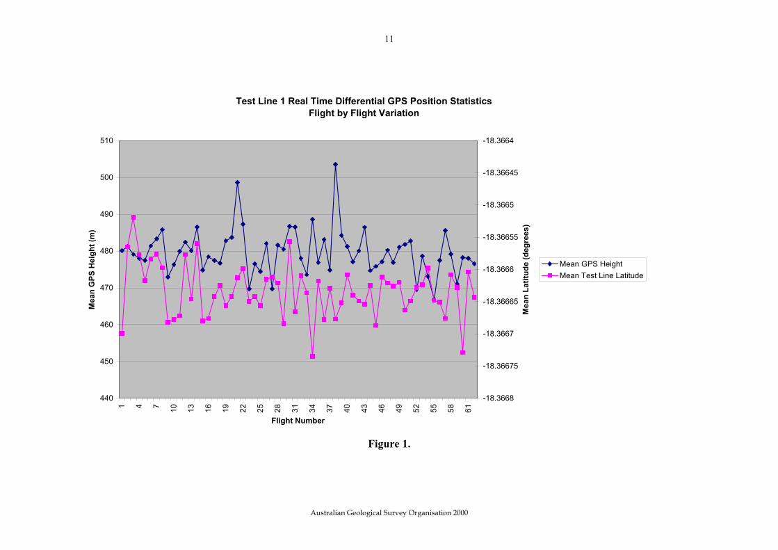
Figure 1. Test Line 1 Real Time Differential GPS Position Statistics ............. 11

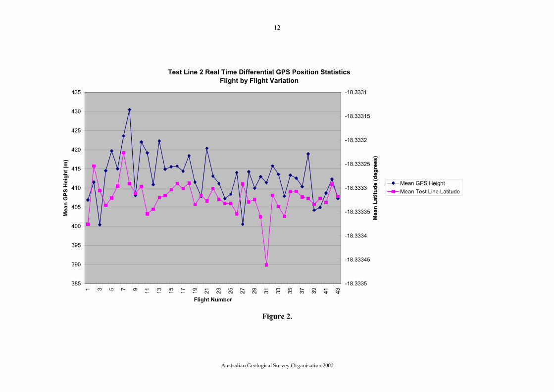
Figure 2. Test Line 2 Real Time Differential GPS Position Statistics ............. 12

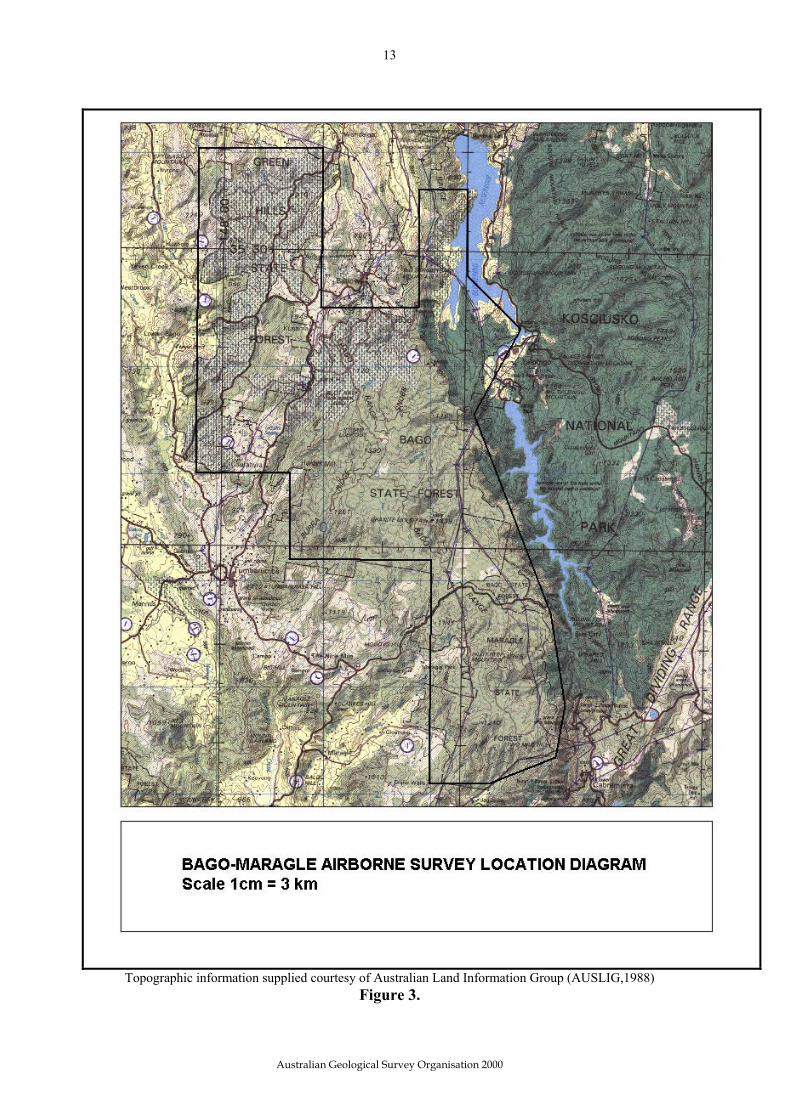
Figure 3. Bago-Maragle Airborne Survey Location Diagram ......................... 13

Figure 4. Bago-Maragle Airborne Geophysical Survey 1996 ......................... 14

Figure 5. Bago-Maragle Line 11100 ................................................................... 15

Figure 6. Results of radar altimeter signal scattering on the final DEM........ 16

Figure 7. Aerial photograph of the area in Figure 6 ......................................... 16

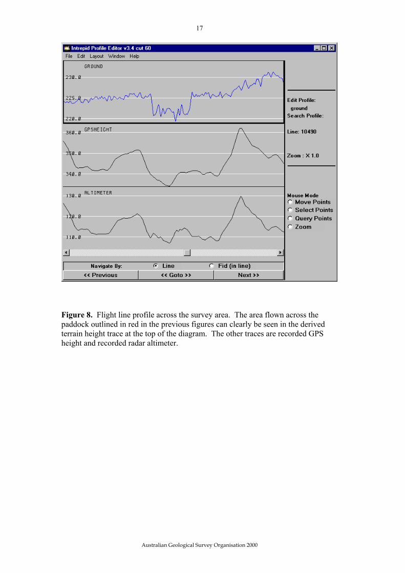
Figure 8. Flight line profile across the survey area........................................... 17

Figure 9. Georgetown Airborne Geophysical Survey DEM............................. 18

References .............................................................................................................. 19

1

Errors in digital elevation models derived from airborne geophysical survey data

1. Introduction A digital elevation model (DEM) is a digital representation of the height of the terrain usually interpolated onto a regularly spaced grid. Traditionally, DEMs have been estimated from ground surveys, digitised topographic maps, satellite (SPOT) images and aerial photography. Since the advent of the Global Positioning System (GPS) for aircraft navigation, DEMs can be derived from positional and aircraft radar altimeter data recorded on airborne geophysical surveys. A DEM is useful in any situation where knowledge of the height, slope and aspect of the ground is important. DEMs are widely used in the following landscape studies – botanical, geochemical, environmental, forest, soil, geological, climatological, geophysical, glaciological and natural hazard (eg landslide). Florinsky (1988) gives a comprehensive list of applications for DEMs. These include: • stream flow modelling • landscape analysis • land use and soil mapping • geological/geophysical mapping • road design and other engineering projects

Although DEMs have been derived from airborne geophysical survey data for several years, there is little information available on the precision and accuracy of these models. The purpose of this paper is to review the procedure for generating an airborne geophysical survey DEM and to investigate the sources and amplitudes of errors in these models. 2. GPS Fundamentals GPS was developed in the 1980s by the U.S. Department of Defence to enable accurate navigation. The GPS satellite constellation consists of twenty-one satellites approximately 20200 km above the earth and uses radio frequencies to transmit the satellite signals between satellite and receiver. The basic principle of GPS is the use of satellites as reference points for triangulating position on the

Australian Geological Survey Organisation 2000

2

earth. Signals from a minimum of four satellites allows the calculation of the position of the receiving antenna. The accuracy in GPS positioning can be increased using a technique called “differential GPS”. In this case a second stationary GPS receiver is placed at a known location allowing the errors in the satellite data to be estimated. These errors can be calculated either after the data have been collected (post-processed differential GPS - DGPS) or during data collection (real time differential GPS - RTDGPS). In real time differential GPS an error correction is transmitted to remote GPS receivers so that the receivers can correct the position solution in real time. Selective Availability (SA) was the intentional modification of the publicly available GPS signal to degrade positional accuracy. On May 2nd 2000 the US government announced that the SA feature would be removed. This means that civilian users will be able to locate their position up to ten times more accurately than was previously possible using one GPS receiver 3. Airborne Geophysical DEM - Methodology The Australian Geological Survey Organisation (AGSO) used GPS navigation for its airborne geophysical surveys from 1991. Once every half second along each survey line the position with respect to the WGS84 ellipsoid (longitude, latitude, height) of the aircraft GPS antenna was calculated by a GPS receiver in the aircraft. The accuracy of the calculated position was claimed by the manufacturer to be better than one metre using RTDGPS. AGSO used RTGPS for aircraft navigation as this allowed the pilot to maintain aircraft tracking using positional data that have been differentially corrected. The real time differential method supplies differential GPS corrections to the satellite range data received in the aircraft via a radio or satellite link from one or more ground based GPS monitoring stations. Flight-line tracking via this method is more precise than by the single GPS receiver method. As a check on the real time differential GPS system and to ensure accurate position information was recorded, the GPS data were post-processed using a GPS base station located at the survey base for the duration of the survey. The location of the base station must be calculated correctly to ensure positional accuracy for the post-processed longitude, latitude and GPS height data. The height of the aircraft above ground level is estimated from a radar altimeter every one second. The raw ground elevation data are calculated as the difference between the height of the aircraft above the ellipsoid (GPS height) and the height of the aircraft above the ground (radar altimeter height). These raw elevation data are calculated every half-second (35 metres along the ground) and are relative to the WGS84 reference ellipsoid.


3

The heights relative to the WGS84 ellipsoid are converted to heights relative to the geoid by subtracting the geoid-ellipsoid separation or N value. The elevation data are then corrected for the vertical separation between the antenna of the aircraft GPS receiver, on the roof of the aircraft, and the radar altimeter antenna on the belly of the aircraft. Richardson (1999) outlines the DEM creation procedure in more detail. The final step is to grid the data by interpolating the corrected DEM profile data onto a regularly spaced grid. 4. Sources of error Using the data recorded during the Georgetown and Bago-Maragle airborne geophysical surveys as examples I will illustrate some of the sources of error in generating airborne geophysical survey DEMs. 4.1 Global Positioning System The United States Air Force, the operator of GPS, defines signal specifications for the GPS system. Under conditions of selective availability a single horizontal GPS position will have an uncertainty of 100 metres at 95% confidence increasing to 300 metres at 99% confidence. The height determined in non-differential mode will have an uncertainty of 156 metres at 95% confidence, rising to 500 metres at 99% confidence. Errors in positioning originate from the following: selective availability, satellite and receiver clocks, tropospheric and ionospheric delays, multipath reflections, receiver noise and satellite geometry. Differential GPS reduces the effects of these errors and provides improved accuracy to the order of several metres. Note that calculated horizontal positions are more accurate than associated ellipsoidal heights because of the influence of satellite geometry on vertical positions. Some of the errors listed above influence the vertical component much more than the horizontal component. A rule of thumb is that the ellipsoidal height accuracy is 1.5 times worse than the horizontal accuracy (Natural Resources Canada, 1995). When acquiring airborne geophysical data a special line called a test line is flown at the beginning and end of each production flight. This line is flown at survey altitude along an identifiable feature (eg. road or fence) for a distance of approximately 10 kilometres and is used for detecting any irregularities in the gamma-ray spectrometric data.


4

Statistics on the Georgetown test line GPS data give an indication of the errors associated with horizontal and vertical positioning. The test line had a bearing of due east/west. The positioning errors are listed in the following table: Mean Northing – std dev. Mean GPS Height – std dev Eastern test line 7 967 281.676 – 5.748 479.759 – 6.174 Western test line 7 971 283.435 – 3.230 412.940 – 3.930 The results show that for each test line over the same terrain the error in vertical accuracy of the aircraft is worse than the horizontal accuracy. 4.2 Altimeter Most surveys conducted by AGSO were flown at 60, 80 or 100 metres above ground level and at 100, 200 or 400 metre flight line spacing depending on the minimum wavelength anomaly to be recorded in the survey area. To maintain a constant ground clearance survey aircraft are fitted with radar altimeters to assist the pilot in maintaining a constant ground clearance and for later processing of the geophysical data. The accuracy of the radar altimeter is claimed by the manufacturer to be ± 2% of the survey height. Thus errors in height from the radar altimeter will be in the range 1.2-2 metres. The radar altimeter signal travels in a perpendicular direction from an antenna on the belly of the aircraft towards the ground. A radar altimeter indicates the actual aircraft height over the terrain. It operates by sending either continuous or pulsed radio signals from a transmitting antenna on the aircraft to the earth’s surface. A receiving antenna on the aircraft then picks up the reflection of the signals from the earth’s surface. The time it takes for the signals to travel to the earth and back is then converted into an absolute altitude. Errors in the recorded altimeter value arise when the reflections of the radar altimeter signal do not originate from the terrain. Under certain conditions the altimeter signal can be reflected from objects above the earths surface. For example, the signal cannot penetrate areas of dense vegetation cover. In densely forested areas the signal is reflected from the forest canopy, and the errors in the estimated aircraft altitude could be 20 metres or more. Signal reflections from man made objects such as large buildings (sheds) also result in errors in the recorded altimeter height for the aircraft. These errors in the radar altimeter data are checked by comparison with the video record of the aircraft’s flight path and edited from the altimeter data if necessary. 4.3 GPS base station location The base station GPS receiver position is accurately determined by differential GPS surveying using a fixed reference point. The horizontal and vertical datums used to locate the fixed reference mark must be known as any errors can seriously degrade


5

the absolute positional accuracy of the entire survey dataset. Most reference marks in Australia are horizontally located with respect to the AGD84 or GDA94 geodetic datums. The vertical datum used is the Australian Height Datum (AHD) that measures height with respect to mean sea level (National Mapping Council of Australia, 1986). An understanding of the difference between a benchmark and a trigonometric mark is important at this point. A relatively permanent marked point whose elevation above or below an adopted datum is known is called a benchmark. A benchmark has an accurate vertical position but comparatively poor horizontal positioning. A trigonometric, or trig, mark is a relatively permanent marked point whose horizontal position on an adopted datum is known. A trig mark has an accurate horizontal position but comparatively poor vertical positioning. The origin of the survey mark must be known, as this affects the horizontal accuracy when a survey point is being used to locate a GPS base station. Knowledge of whether the point is a benchmark or a trig mark is also essential when assessing the height errors in the final DEM. Any reference mark must be transformed into the WGS84 datum with an associated ellipsoidal height calculated using the following formula:

H = h - N ------------------- (1) where

H = height above the geoid (mean sea level or orthometric height); h = height above the ellipsoid (ellipsoidal height); and N = Geoid – ellipsoid separation (N value). If the geoid is above the ellipsoid, N is positive If the geoid is below the ellipsoid, N is negative

An N value is specific to a particular ellipsoid and care must be taken to ensure that the N value refers to the correct ellipsoid (Johnston & Featherstone, 1998.). AGSO uses the AUSGeoid98 national geoid model produced by the Australian Surveying and Land Information Group (AUSLIG). The WGS84 N values range from –40 to +70 m across Australia. Failure to apply this transformation to X, Y and Z will result in position errors up to approximately 200 metres to any DEM generated from airborne geophysical navigation data. 4.4 Gridding (interpolation) A position sample (X, Y and Z) is usually recorded every 0.5 seconds in an airborne geophysical survey. At a nominal survey aircraft speed of 70 ms-1 each flight line will have a terrain height value approximately every 35 metres along the flight line. Perpendicular to the flight line the terrain sampling will be equivalent to the flight line spacing. Thus the geophysical survey method has high terrain data sampling density along the flight lines but only sparse sampling density perpendicular to the


6

flight lines. This may lead to interpolation errors if the terrain elevation exhibits ruggedness between the flight lines (Kennett and Eiken, 1997). AGSO digital elevation models are calculated using interpolation software that applies sensible drainage conditions by calculating drainage constraints from stream line data during the gridding process (Hutchinson, 1988,1999). The effect of gridding can be illustrated by comparing the airborne terrain profile data with the gridded data. The following table shows the DEM data for a traverse line (segment 2600), tie line (segment 380) and the DEM grid along the position of the line/tie. Statistics on the differences are listed in the following table:

Difference between traverse/tie line terrain profiles and DEM grid profile No. data pts Mean Diff. Std. Dev. Length (km) Line Direction Tie 2930 -2.35 5.61 108.4 East-West Traverse 3200 0.56 1.51 114.2 North-South The Georgetown airborne geophysical survey has a flight line spacing of 200 metres, a tie line spacing of 2000 metres, and a grid cell size of 40 metres. The tie lines are not included in the gridding process so in the north-south direction the traverse lines provide a real data sample every 200 metres that is interpolated onto a cell size of 40 metres. The large standard deviaitions for the tie line illustrate the effect of low terrain data sampling in that direction. The tie line has a sample every 70 metres whereas the DEM grid has a real data sample every 200 metres in that direction (grid samples are interpolated to a 40 metre sample interval). 4.5 Levelling There are day – to – day variations in the GPS heights recorded in the aircraft when flying over the same piece of ground. This is illustrated in the terrain profiles recorded along the gamma-ray spectrometric test lines flown at the beginning and end of each day’s production flying (Figures 1 & 2). The figures illustrate that GPS height can vary from flight to flight by up to 20 metres. To remove these effects the data are levelled using standard tie line levelling procedures. Luyendyk (1997) describes the procedure for the tie line levelling method in more detail. The DEM profile data are also microlevelled using a procedure developed by Minty (1991) to remove any residual errors after the tie line levelling process. Care must be taken when microlevelling DEM profile data as real terrain features that are parallel to the flight-line direction can be removed when the only features targeted for removal are the residual errors that are elongate along the flight-line direction. 4.6 Cultural Effects The effect of man made obstacles is evident in the raw data recorded on the Bago – Maragle airborne geophysical survey flown in 1996. A survey location diagram is shown in Figure 3. In order to fly over the location of high tension power lines in


7

the eastern side of the survey area the aircraft increased terrain clearance, and consequently GPS height. This feature is illustrated in both the raw altimeter and GPS height grids shown in Figure 4. A linear feature in the form of an inverted ‘Y’ can be seen on the right hand side of these grids. The final DEM data are shown at the bottom of Figure 4 with no obvious imprint of the power line location in the image. Is the final DEM data representative of the terrain at the location of the power lines? A flight line that tracked over the power lines was chosen for further investigation. Line 11100 is situated over the southwestern corner of Blowering Reservoir, where the aircraft intercepts hilly terrain and flies over the power line (Figure 5). The altimeter data indicates that the aircraft starts climbing at fiducial 44520, levels out for a short while between fiducials 44610 and 44630 then resumes climbing before levelling out around fiducial 44670. At the same time as the altimeter data levels out for a short time the GPS height data is steadily increasing. This indicates that the ground underneath the aircraft exhibits a constant slope but the terrain ahead still requires an increase in aircraft terrain clearance, deduced from increasing GPS height. The final DEM profile data does not appear to be influenced by the locations of the power lines in this example. To investigate the underlying behaviour of the altimeter, GPS height and ground data chains the first difference was calculated for each data value. These calculations are also displayed in Figure 5. The first difference is calculated by subtracting adjacent samples of each data chain from one another. The results indicate the difference in value from the current sample to the previous sample for each data sample. In Figure 5 at fiducial 45600 the first difference of altimeter starts to decrease rapidly and the first difference of ground starts to increase rapidly yet the first difference of GPS height is fairly constant. The fairly constant first difference of GPS height indicates that the aircraft is not ascending or descending too rapidly. The change in first difference of altimeter at fiducial 44600 indicates the distance between the aircraft and the ground is decreasing due to rising terrain underneath the flight path of the aircraft. This effect until fiducial 44620 before a trend reversal – the first difference of altimeter starts to increase and the first difference of ground starts to decrease. That is, the ground starts to level out underneath the flight path of the aircraft causing the terrain clearance (altimeter reading) between the aircraft and the ground to increase. In areas of flat terrain the first difference of altimeter would be zero. To enhance the clarity of the graph in Figure 5 a constant value of 80 was added to all the first difference calculations. An example of radar altimeter signal scattering is shown in figures 6, 7 and 8. The gridded profile data is shown in figure 6. The ground elevation is fairly flat except for a few hills coloured red and yellow. There are a number of rectangular depressions depicted coloured dark blue. These are due to paddocks. One of these is outlined and is clearly evident in the centre of the figure. Figure 7 is an aerial photograph of the central area with the paddock outlined. In figure 8 a profile of the


8

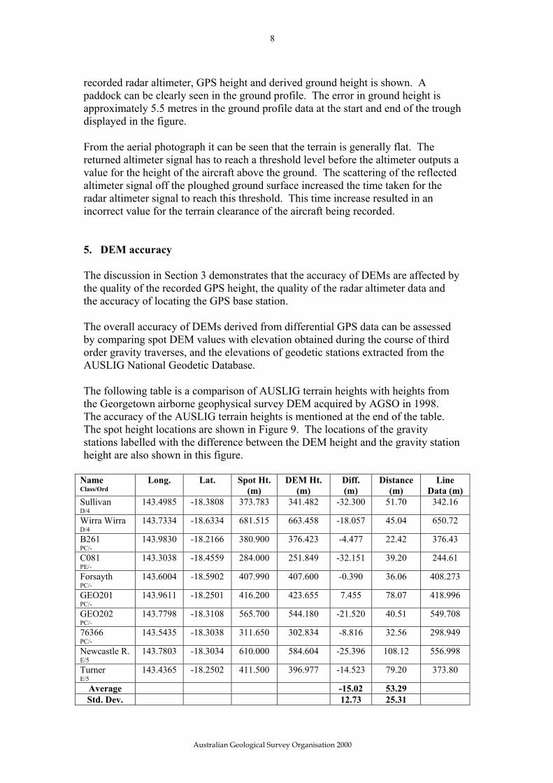
recorded radar altimeter, GPS height and derived ground height is shown. A paddock can be clearly seen in the ground profile. The error in ground height is approximately 5.5 metres in the ground profile data at the start and end of the trough displayed in the figure. From the aerial photograph it can be seen that the terrain is generally flat. The returned altimeter signal has to reach a threshold level before the altimeter outputs a value for the height of the aircraft above the ground. The scattering of the reflected altimeter signal off the ploughed ground surface increased the time taken for the radar altimeter signal to reach this threshold. This time increase resulted in an incorrect value for the terrain clearance of the aircraft being recorded. 5. DEM accuracy The discussion in Section 3 demonstrates that the accuracy of DEMs are affected by the quality of the recorded GPS height, the quality of the radar altimeter data and the accuracy of locating the GPS base station. The overall accuracy of DEMs derived from differential GPS data can be assessed by comparing spot DEM values with elevation obtained during the course of third order gravity traverses, and the elevations of geodetic stations extracted from the AUSLIG National Geodetic Database. The following table is a comparison of AUSLIG terrain heights with heights from the Georgetown airborne geophysical survey DEM acquired by AGSO in 1998. The accuracy of the AUSLIG terrain heights is mentioned at the end of the table. The spot height locations are shown in Figure 9. The locations of the gravity stations labelled with the difference between the DEM height and the gravity station height are also shown in this figure.

Name Class/Ord

Long. Lat. Spot Ht. (m)

DEM Ht. (m)

Diff. (m)

Distance (m)

Line Data (m)

Sullivan D/4

143.4985 -18.3808 373.783 341.482 -32.300 51.70 342.16

Wirra Wirra D/4

143.7334 -18.6334 681.515 663.458 -18.057 45.04 650.72

B261 PC/-

143.9830 -18.2166 380.900 376.423 -4.477 22.42 376.43

C081 PE/-

143.3038 -18.4559 284.000 251.849 -32.151 39.20 244.61

Forsayth PC/-

143.6004 -18.5902 407.990 407.600 -0.390 36.06 408.273

GEO201 PC/-

143.9611 -18.2501 416.200 423.655 7.455 78.07 418.996

GEO202 PC/-

143.7798 -18.3108 565.700 544.180 -21.520 40.51 549.708

76366 PC/-

143.5435 -18.3038 311.650 302.834 -8.816 32.56 298.949

Newcastle R. E/5

143.7803 -18.3034 610.000 584.604 -25.396 108.12 556.998

Turner E/5

143.4365 -18.2502 411.500 396.977 -14.523 79.20 373.80

Average -15.02 53.29 Std. Dev. 12.73 25.31


9

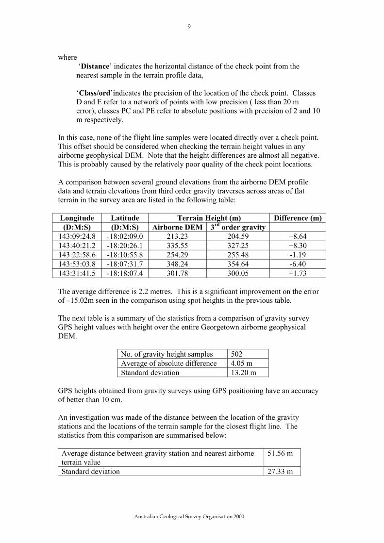
where ‘Distance’ indicates the horizontal distance of the check point from the nearest sample in the terrain profile data, ‘Class/ord’indicates the precision of the location of the check point. Classes D and E refer to a network of points with low precision ( less than 20 m error), classes PC and PE refer to absolute positions with precision of 2 and 10 m respectively.

In this case, none of the flight line samples were located directly over a check point. This offset should be considered when checking the terrain height values in any airborne geophysical DEM. Note that the height differences are almost all negative. This is probably caused by the relatively poor quality of the check point locations. A comparison between several ground elevations from the airborne DEM profile data and terrain elevations from third order gravity traverses across areas of flat terrain in the survey area are listed in the following table: Longitude Latitude Terrain Height (m) Difference (m) (D:M:S) (D:M:S) Airborne DEM 3rd order gravity

143:09:24.8 -18:02:09.0 213.23 204.59 +8.64 143:40:21.2 -18:20:26.1 335.55 327.25 +8.30 143:22:58.6 -18:10:55.8 254.29 255.48 -1.19 143:53:03.8 -18:07:31.7 348.24 354.64 -6.40 143:31:41.5 -18:18:07.4 301.78 300.05 +1.73 The average difference is 2.2 metres. This is a significant improvement on the error of –15.02m seen in the comparison using spot heights in the previous table. The next table is a summary of the statistics from a comparison of gravity survey GPS height values with height over the entire Georgetown airborne geophysical DEM.

No. of gravity height samples 502 Average of absolute difference 4.05 m Standard deviation 13.20 m

GPS heights obtained from gravity surveys using GPS positioning have an accuracy of better than 10 cm. An investigation was made of the distance between the location of the gravity stations and the locations of the terrain sample for the closest flight line. The statistics from this comparison are summarised below: Average distance between gravity station and nearest airborne terrain value

51.56 m

Standard deviation 27.33 m


10

6. Conclusions DEM accuracy is affected by both random and systematic errors. Random errors include the height data calculated by the GPS receiver in the aircraft and the attitude/stability of the aircraft. Systematic errors include the interpolation and microlevelling processes and the quality of the returned radar altimeter signal to the aircraft. The errors contained in a DEM are of the order of approximately 10 metres. The main contributions are from the radar altimeter data (1-2 metres) and the GPS height data (5-10 metres). The GPS satellite constellation visible by the GPS receiving antenna is the major cause for error in GPS height calculations. When height comparisons are made in areas of flat terrain the errors are of the order of approximately 2 metres. Consideration should be given to the source datasets (radar altimeter, GPS) used to derive a DEM. As was illustrated in the paddock example, a digital elevation model cannot be guaranteed to be a true representation of the ground height above sea level. However, as a by-product from the GPS navigation data recorded on an airborne geophysical survey, airborne digital elevation data is a relatively cheap and accurate model of the topography of an area. With the removal of Selective Availability from the GPS satellite signal the accuracy of GPS positioning will be improved tenfold.


11

Test Line 1 Real Time Differential GPS Position StatisticsFlight by Flight Variation

440

450

460

470

480

490

500

510

1 4 7 10 13 16 19 22 25 28 31 34 37 40 43 46 49 52 55 58 61

Flight Number

Mea

n G

PS H

eigh

t (m

)

-18.3668

-18.36675

-18.3667

-18.36665

-18.3666

-18.36655

-18.3665

-18.36645

-18.3664

Mea

n La

titud

e (d

egre

es)

Mean GPS HeightMean Test Line Latitude

Figure 1.


12

Test Line 2 Real Time Differential GPS Position StatisticsFlight by Flight Variation

385

390

395

400

405

410

415

420

425

430

4351 3 5 7 9 11 13 15 17 19 21 23 25 27 29 31 33 35 37 39 41 43

Flight Number

Mea

n G

PS H

eigh

t (m

)

-18.3335

-18.33345

-18.3334

-18.33335

-18.3333

-18.33325

-18.3332

-18.33315

-18.3331

Mea

n La

titud

e (d

egre

es)

Mean GPS HeightMean Test Line Latitude

Figure 2.


13

Topographic information supplied courtesy of Australian Land Information Group (AUSLIG,1988)

Figure 3.


14

Figure 4.


15

BAGO-MARAGLE LINE 11100

350

400

450

500

550

600

4450

0

4452

0

4454

0

4456

0

4458

0

4460

0

4462

0

4464

0

4466

0

4468

0

4470

0

4472

0

4474

0

4476

0

4478

0

4480

0

4482

0

4484

0

4486

0

4488

0

4490

0

Fiducial

GPS

Hei

ght (

met

res)

60

70

80

90

100

110

120

130

140

150

160Along line distance: 1110 m (approx)

Alti

met

er H

eigh

t (m

etre

s)

Ground (LHS)GPS Height (LHS)Altimeter (RHS)First Diff Ground + constant (RHS)First Diff Altimeter + constant (RHS)First Diff GPS Height + constant (RHS)

Figure 5.


16

Figure 6. Results of radar altimeter signal scattering on the final airborne geophysical survey digital elevation model. The outlines of several paddocks are clearly seen.


Figure 7. Aerial photograph of the area in figure 6. The area of interest is outlined in red.

17


Figure 8. Flight line profile across the survey area. The area flown across the paddock outlined in red in the previous figures can clearly be seen in the derived terrain height trace at the top of the diagram. The other traces are recorded GPS height and recorded radar altimeter.

18

Figure 9.


19


References AUSLIG., 1988. – Wagga Wagga 1:250 000 Joint Operations Graphic topographic map. Series 1501, Edition 1. Sheet SI55-15 Florinsky, I.V., 1988. – Combined analysis of digital terrain models and remotely sensed data in landscape investigations. Progress in Physical Geography, 22, 1, 33-60. Hutchinson, M.F., 1988. – Calculation of hydrologically sound digital elevation models. Third International Symposium on Spatial Data Handling, Sydney. International Geographical Union, Columbus, 117-133. Hutchinson, M.F., 1989. – A new procedure for gridding elevation and stream line data with automatic removal of spurious pits. Journal of Hydrology, 106, 211-232. Johnston, G.M. and Featherstone, W.E., 1998. – AUSGeoid98: A new gravimetric geoid for Australia. Paper presented to the 24th National Surveying Conference of the Institution of Engineering and Mining Surveyors, 27th September – 3rd October, 1998. http://www.auslig.gov.au/techpap/iemsgary.pdf Kennet, M. and Eiken, T., 1997. – Airborne measurement of glacier surface elevation by scanning laser altimeter. Annal of Glaciology, 24, 293-296. Luyendyk, A., 1997. – Processing of airborne magnetic data. AGSO Journal of Australian Geology and Geophysics, 17(2), 23-30. Minty, B.R.S., 1991 – Simple micro-levelling for aeromagnetic data. Exploration Geophysics. 22, 591-592 National Mapping Council of Australia, 1986. – The Australian Geodetic Datum Technical Manual. Special Publication No. 10. Natural Resources Canada, 1995. – GPS Positioning Guide (third edition). Richardson, L.M., 1999. – Georgetown, Qld Airborne Geophysical Survey, 1998 Operations Report. Australian Geological Survey Organisation, Record 1999/13.

Errors in digital elevation models derived from airborne ... can be derived from positional and...

Documents

Transcript of Errors in digital elevation models derived from airborne ... can be derived from positional and...