Enterprise-wide optimization for the fast movingconsumer goods industryvan Elzakker, M.A.H.

DOI:10.6100/IR760961

Published: 01/01/2013

Document VersionPublisher’s PDF, also known as Version of Record (includes final page, issue and volume numbers)

Please check the document version of this publication:

• A submitted manuscript is the author's version of the article upon submission and before peer-review. There can be important differencesbetween the submitted version and the official published version of record. People interested in the research are advised to contact theauthor for the final version of the publication, or visit the DOI to the publisher's website.• The final author version and the galley proof are versions of the publication after peer review.• The final published version features the final layout of the paper including the volume, issue and page numbers.

Link to publication

Citation for published version (APA):Elzakker, van, M. A. H. (2013). Enterprise-wide optimization for the fast moving consumer goods industryEindhoven: Technische Universiteit Eindhoven DOI: 10.6100/IR760961

General rightsCopyright and moral rights for the publications made accessible in the public portal are retained by the authors and/or other copyright ownersand it is a condition of accessing publications that users recognise and abide by the legal requirements associated with these rights.

• Users may download and print one copy of any publication from the public portal for the purpose of private study or research. • You may not further distribute the material or use it for any profit-making activity or commercial gain • You may freely distribute the URL identifying the publication in the public portal ?

Take down policyIf you believe that this document breaches copyright please contact us providing details, and we will remove access to the work immediatelyand investigate your claim.

Download date: 17. Jun. 2018

Enterprise-Wide Optimization

for the

Fast Moving Consumer Goods Industry

M.A.H. van Elzakker

Doctoral Committee Chairman prof.dr.ir. J.C. Schouten Eindhoven University of Technology 1st Promoter prof.dr. I.E. Grossmann Carnegie Mellon University, Pittsburgh 2nd Promoter prof.dr. J. Meuldijk Eindhoven University of Technology Co-Promoter dr.ir. E. Zondervan Eindhoven University of Technology Examiners prof.dr. N. Shah Imperial College London prof.dr.ir. J.C. Fransoo Eindhoven University of Technology prof.ir. J. Grievink Delft University of Technology dr. C. Almeida-Rivera Unilever

Enterprise-Wide Optimization for the Fast Moving Consumer Goods Industry Martijn A.H. van Elzakker A catalogue record is available from the Eindhoven University of Technology Library ISBN: 978-90-386-3494-4 Cover design by Esther Ris, www.proefschriftomslag.nl Printed by Gildeprint Drukkerijen, www.gildeprint.nl

The research described in this thesis was supported by Unilever Copyright © M.A.H. van Elzakker, the Netherlands, 2013 All rights reserved

Enterprise-Wide Optimization

for the

Fast Moving Consumer Goods Industry

PROEFSCHRIFT

ter verkrijging van de graad van doctor aan de Technische Universiteit Eindhoven, op gezag van de rector magnificus prof.dr.ir. C.J. van Duijn,

voor een commissie aangewezen door het College voor Promoties, in het openbaar te verdedigen op woensdag 11 december 2013 om 14:00 uur

door

Marinus Antonius Hendricus van Elzakker

geboren te Bergen op Zoom

Dit proefschrift is goedgekeurd door de promotoren en de samenstelling van de promotiecommissie is als volgt:

voorzitter: prof.dr.ir. J.C. Schouten 1e promotor: prof.dr. I.E. Grossmann (Carnegie Mellon University) 2e promotor: prof.dr. J. Meuldijk copromotor: dr.ir. E. Zondervan leden: prof.dr. N. Shah (Imperial College London) prof.dr.ir. J.C. Fransoo prof.ir. J. Grievink (Delft University of Technology) adviseur: dr. C. Almeida-Rivera (Unilever)

Summary

i

Summary

Enterprise-Wide Optimization for the Fast Moving Consumer Goods Industry

Because of the increasingly competitive global market, companies with a global supply chain have to continuously evaluate and optimally reconfigure their supply chain operations. Optimizing the supply chain involves balancing many different aspects. For example, while centralized production may benefit from the economies of scale, local production will reduce the transportation costs. Enterprise-Wide Optimization (EWO) is similar to supply chain optimization, although with a greater emphasis on the production facilities. In addition to the usual challenges associated with EWO, Fast-Moving Consumer Goods (FMCG) companies must also consider an extremely large number of products and the seasonality of those products and their ingredients.

Due to the complexity of the supply chain, spreadsheet optimization is unlikely to result in the best possible configuration and operation. Instead, the integrated supply chain can be optimized by using Mathematical Programming (MP) models. The main objective of this thesis is to develop MP models that can be used to optimize the supply chain operations of a FMCG company.

First, a short-term scheduling Mixed-Integer Linear Programming (MILP) model is developed. In this model, the timing and allocation decisions are optimized for a single factory over a one week horizon. The computational efficiency is increased by exploiting the problem characteristics. For example, the number of binary variables is decreased drastically by dedicating time intervals to product types. As a result, the weekly planning for a small factory can be optimized within 170 seconds. Next, a periodical cleaning requirement is added to this scheduling model. While this significantly increases the complexity of the model, it can still be optimized within a reasonable time using a proposed algorithm. Using this algorithm, for 9 out of 10 case studies an optimal solution can be obtained within half an hour. The makespan in the 10th case study is 0.6% higher than the theoretical minimum makespan.

Secondly, a tactical planning MILP model is developed. In the tactical planning model, the complete supply chain is considered over a one year horizon. The main decisions are procurement, production, product set-up, inventory, and distribution. While this model is demonstrated for a case study containing 10 Stock-Keeping Units (SKUs), it becomes intractable for larger, more realistically sized problems.

Therefore, an algorithm based on decomposing the model into single-SKU submodels is proposed. To account for the interaction between SKUs, slack variables are introduced into the capacity constraints. These slack variables initially allow the capacity to be violated. In

Summary

ii

an iterative procedure the cost of violating the capacity is slowly increased, and eventually a feasible solution is obtained. Even for a relatively small 10-SKU case study, the required CPU time can be reduced from 1144 to 175 seconds using the decomposition algorithm. Moreover, the algorithm is used to optimize case studies containing up to 1000 SKUs, whereas the full space model is intractable for case studies containing 50 or more SKUs. The solutions obtained with the algorithm are typically within a few percent of the global optimum.

Thirdly, shelf-life restrictions are incorporated into this tactical planning problem. It is crucial to consider the shelf-life, since otherwise products in inventory could exceed their shelf-life, which would lead to unnecessary waste and possibly missed sales due to the reduced inventory level. Three possible methods for considering the shelf-life are evaluated. The direct method tracks the age of all products. It can guarantee optimal solutions, but it is computationally inefficient. The indirect method ensures all products leave the supply chain before the end of their shelf-life without tracking the age of individual products. It is the most efficient method, and it typically finds solutions within a few percent of optimality. The hybrid method combines the direct and indirect methods, has an average computational efficiency, and obtains near optimal solutions.

Finally, the environmental impact is introduced into the tactical planning model using the Eco-indicator 99 system. The trade-offs between environmental and economic objectives of operating the supply chain are evaluated using a Pareto analysis. A set of solutions approximating the Pareto front is generated using the -constraint method. Since the tactical planning decisions are often optimized within a specified optimality tolerance of for example 1%, the environmental impact can typically be reduced by a few percent without increasing the economic costs. The main opportunities for reducing the environmental impact are related to the supplier and factory decisions.

Overall it can be concluded that while EWO problems in the FMCG industry are typically large and complex, good solutions can be obtained by using efficient mathematical programming models combined with decomposition algorithms.

Table of Contents

iii

Table of Contents

SUMMARY i

1. INTRODUCTION 1 1.1. SCHEDULING................................................................................................................. 3 1.2. TACTICAL PLANNING.................................................................................................... 8 1.3. MIXED INTEGER LINEAR PROGRAMMING................................................................... 11 1.4. OBJECTIVES................................................................................................................ 14 1.5. OUTLINE..................................................................................................................... 15

2. SCHEDULING 19 2.1. INTRODUCTION........................................................................................................... 20 2.2. PROBLEM DEFINITION................................................................................................ 21 2.3. DEDICATED TIME INTERVALS..................................................................................... 23 2.4. INVENTORY................................................................................................................ 25 2.5. RELATED INTERVAL METHOD (RIM)......................................................................... 25 2.6. STN MODEL............................................................................................................... 35 2.7. RESULTS..................................................................................................................... 36 2.8. CONCLUSIONS............................................................................................................ 48 2.9. NOMENCLATURE........................................................................................................ 48

3. TACTICAL PLANNING 51 3.1. INTRODUCTION........................................................................................................... 52 3.2. PROBLEM DEFINITION................................................................................................ 54 3.3. MILP MODEL FORMULATION...................................................................................... 55 3.4. CASE STUDIES............................................................................................................ 60 3.5. RESULTS..................................................................................................................... 61 3.6. CONCLUSIONS............................................................................................................ 63 3.7. NOMENCLATURE........................................................................................................ 64

4. SKU-DECOMPOSITION ALGORITHM 67 4.1. INTRODUCTION........................................................................................................... 68 4.2. SKU-DECOMPOSITION ALGORITHM........................................................................... 69 4.3. SUBMODEL CONSTRAINTS.......................................................................................... 72

Table of Contents

iv

4.4. ILLUSTRATIVE EXAMPLE............................................................................................ 77 4.5. RESULTS..................................................................................................................... 80 4.6. CONCLUSIONS............................................................................................................ 90 4.7. NOMENCLATURE........................................................................................................ 91

5. SHELF-LIFE 95 5.1. INTRODUCTION........................................................................................................... 96 5.2. PROBLEM DEFINITION................................................................................................ 98 5.3. SHELF-LIFE................................................................................................................. 98 5.4. RESULTS................................................................................................................... 108 5.5. CONCLUSIONS.......................................................................................................... 116 5.6. NOMENCLATURE...................................................................................................... 116

6. ENVIRONMENTAL IMPACT 121 6.1. INTRODUCTION......................................................................................................... 122 6.2. PROBLEM DEFINITION.............................................................................................. 124 6.3. ENVIRONMENTAL IMPACT........................................................................................ 124 6.4. THE -CONSTRAINT METHOD.................................................................................. 128 6.5. RESULTS................................................................................................................... 130 6.6. CONCLUSIONS.......................................................................................................... 139 6.7. NOMENCLATURE...................................................................................................... 140

7. CONCLUSIONS AND OUTLOOK 143 7.1. CONCLUSIONS.......................................................................................................... 144 7.2. MAIN CONTRIBUTIONS............................................................................................. 146 7.3. OUTLOOK................................................................................................................. 147

APPENDICES I

REFERENCES VII

ACKNOWLEDGEMENTS XIX

LIST OF PUBLICATIONS XXI

CURRICULUM VITAE XXIII

deod

oran

t

1.Introduction

Chapter 1

2

Every day, billions of people worldwide use Fast Moving Consumer Goods (FMCG). These FMCG are typically products one can buy at a supermarket, such as food products, drinks and detergents (Sattler et al., 2010). These products are mostly produced by large multinational companies such as Unilever, Procter & Gamble and Nestlé, which all have a yearly revenue of over €50BN.

These companies produce a wide range of products to satisfy an increasing demand for product variety (Bilgen and Günther, 2010). In fact, even a single product category, such as ice cream, can consist of a thousand Stock-Keeping Units (SKUs). These SKUs are products that may vary in composition or packaging.

Generally, FMCG are fully used up or replaced over a short period of time, ranging from days to months depending on the product (Leahy, 2011). In addition, seasonality plays an important role in the FMCG industry. Not only are the products often seasonal, but many of the ingredients are seasonal as well. In addition, many FMCG have a maximum shelf-life and can, therefore, only be stored for a limited amount of time.

When a FMCG is sold out, a consumer will typically buy a substitute product rather than waiting for the product to become available. This substitute product might very well be a product of one of the competitors. Therefore, it is very important that a sufficient amount of product is available at the retailers.

However, the costs of maintaining a sufficient inventory throughout the supply chain to ensure a high customer service level are generally significant (Papageorgiou, 2009). Even though FMCG are profitable because they are produced and sold in large quantities, they generally have a low profit margin. Therefore, it is crucial to obtain the right balance between minimizing the total costs of operating the supply chain, including inventory costs, and ensuring that a sufficient amount of product is available to meet the demand. However, the scale and complexity of the enterprise-wide supply chains in which these products are produced has increased significantly due to globalization (Varma et al., 2007).

Therefore, Enterprise-Wide Optimization (EWO) has become a major goal in the process industries. EWO is a relatively new research area that lies at the interface of chemical engineering and operations research (Grossmann, 2005). It involves optimizing the procurement, production and distribution functions of a company. Although similar to Supply Chain Management (SCM), it typically places a greater emphasis on the manufacturing facilities. Laínez and Puigjaner (2012) provide a review on EWO and SCM. The major activities included in EWO can be divided into three temporal layers, as is shown in Figure 1.1.

The first layer is strategic planning, which optimizes long term decisions, such as the supply chain design, over a time horizon covering several years. The second layer is tactical planning, which optimizes the procurement, production and distribution activities of a

Introduction

3

supply chain over a shorter time horizon which can range from several weeks up to a year. The third layer is scheduling, which focusses on the short term allocation and timing decisions, typically covering a few days to one or two weeks.

Figure 1.1. Overview of the temporal layers in Enterprise-Wide Optimization

It should be noted that these three temporal layers are, in principle, part of the same problem. Therefore, the interaction between the layers is important. For example, the tactical planning will provide the production targets for the scheduling. However, the production capacity is represented in less detail on the tactical planning layer than on the scheduling level. Nevertheless, the production capacity in the tactical planning should closely resemble the restrictions found on the scheduling level. Otherwise, either suboptimal solutions will be obtained if the production capacity is underestimated, or infeasible production targets will be obtained if the production capacity is overestimated.

The focus in this thesis will be on the tactical planning and short-term scheduling layers. In the remainder of this introduction chapter, the basic concepts of scheduling and tactical planning will first be introduced. Then, a short introduction will be given to Mixed Integer Linear Programming (MILP), which is the model type used to optimize the scheduling and tactical planning problems in this thesis. Finally, the objectives of this thesis will be discussed and an outline of the thesis will be given.

1.1. Scheduling

Scheduling plays an important role in most manufacturing and service industries (Pinedo and Chao, 1999). It involves allocating limited resources to activities such that the objectives of a company are optimized (Pinedo, 2009). Various objectives can be used in

Chapter 1

4

the scheduling. For example, the objective can be to minimize the time to complete all activities, the total tardiness, or the total costs.

The type of scheduling considered in this thesis is short-term production scheduling of a single production facility. The main decisions of production scheduling are to select the tasks to be executed, to decide on which equipment the tasks should be executed, and to determine the sequence and the exact timing of the tasks (Harjunkoski et al., 2013).

Production scheduling has historically been done manually using pen and paper, heuristics, planning cards, or spreadsheets (Harjunkoski et al., 2013). However, especially when the utilization percentage of the equipment is high, the scheduling can become complex, and even obtaining a feasible schedule can become difficult. As a result, optimization support can substantially improve the capacity utilization leading to significant savings. For example, Bongers and Bakker (2006) reported an increase in effective production capacity of 10-30% by using a multistage scheduling model rather than manually scheduling the separate stages in the factory.

A variety of approaches have been developed to facilitate the production scheduling and to improve the solutions. These approaches include expert systems, mathematical programming, and evolutionary algorithms. In chemical engineering, MILP is one of the most commonly used methods for optimizing scheduling problems (Mouret et al., 2009). For example, State-Task Network (STN) (Kondili et al., 1993) and Resource-Task Network (RTN) (Pantelides, 1994) MILP formulations have been applied to a large variety of scheduling problems.

One of the most important characteristics of scheduling models is their time representation. A discrete time model divides the scheduling horizon into a finite number of time slots with a pre-specified length. However, to accurately represent all activities of various length, a fairly short time slot length must typically be used (Floudas and Lin, 2004). As a result, the total number of time slots might be large. Since most variables and constraints are expressed for each time slot, the resulting model can become very large. On the other hand, the advantage of a formulation based on a discrete time horizon is that it is typically tight (Harjunkoski et al., 2013).

A continuous time model also divides the scheduling horizon into a finite number of time slots, but the length of these time slots is determined in the optimization. Therefore, the number of time slots can be reduced considerably, and the resulting models are substantially smaller. Nevertheless, they do not necessarily perform better computationally than discrete time formulations (Harjunkoski et al., 2013). In addition, it can be challenging to determine the optimal number of time slots in a continuous time model.

In a precedence-based model, the tasks are not directly related to a time line, but instead the focus is on binary precedence relationships between tasks executed on the same unit

Introduction

5

(Maravelias, 2012). As a result, precedence-based models can handle sequence dependent changeover times in a straightforward manner. However, the disadvantage of precedence-based models is that the number of sequencing variables scales quadratically with the number of batches to be scheduled (Mendez et al., 2006). As a result, precedence-based models can become relatively large for real-world applications.

Another important characterization of scheduling models is their scope. A generic model aims at addressing a wide variety of problems. On the other hand, in a problem specific formulation the computational efficiency can be increased by using the problem characteristics. However, this often means that the problem specific model relies on these problem characteristics and is, therefore, only applicable to a smaller range of problems. Nevertheless, problem specific formulations can often be used to optimize problems that are too large or complex for generic models.

More extensive reviews on production scheduling are provided by Kallrath (2002b), Floudas and Lin (2004), Mendez et al. (2006), Zhu and Wilhelm (2006), Li and Ierapetritou (2008), Allahverdi et al. (2008), Ribas et al. (2010), Maravelias (2012), and Harjunkoski et al. (2013). In the remainder of this section, an overview of production scheduling in the FMCG industry will be given.

1.1.1. Scheduling in the FMCG Industry

The short-term scheduling problem in the FMCG industry can be characterized as follows: A typical FMCG production process is a two-stage make-and-pack production process with limited intermediate storage (Bilgen and Günther, 2010). This is a sequential process because, as shown in Figure 1.2, each product is first produced on a production line, then stored in one of the storage tanks, and finally packed on one of the packing lines. The production process is usually a semi-continuous process, where storage tanks often determine the batch size. The production targets are usually obtained from the tactical planning. A more detailed description of the production process will be given in Chapter 2.

Wilkinson et al. (1996) optimize the production and distribution scheduling of a FMCG company. They optimize the production of three factories that serve 15 warehouses. They adopt an aggregated formulation (Wilkinson et al., 1995) of the RTN model introduced by Pantelides (1994). This aggregated RTN formulation approximates the production capacity, which greatly reduces the size of the problem. The model is used to determine the transport of products from factories to warehouses. In the second step of their solution procedure, a detailed production plan is established for each factory using the production targets determined in the previous step. Their formulation uses a discrete time horizon with intervals of 2 hours, which effectively means that all tasks must be performed for multiples of 2 hours.

Chapter 1

6

Figure 1.2. Typical production process in the FMCG industry

Mendez and Cerda (2002b) presented an MILP based approach for the scheduling of make-and-pack production plants. They significantly reduced the required computational time by applying preordering rules for both stages, which rely on their assumption of unlimited intermediate storage. Using these preordering rules, they obtained near optimal solutions.

Shaik and Floudas (2007) proposed a unit-specific event-based continuous time STN model for short-term scheduling of continuous processes. They considered unlimited inventory, dedicated finite storage, flexible finite storage, no intermediate storage, and the bypassing of intermediate storage. They compared their model with models of Giannelos and Georgiadis (2002), Castro et al. (2004a and 2004b), and Mendez and Cerda (2002a) for case studies with various inventory requirements based on a FMCG manufacturing process. On average, the model of Shaik and Floudas (2007) was the most efficient, and their model could obtain the global optimal solution for all case studies. astro et alCastro et al.

Soman et al. (2007) evaluate a previously developed hierarchical production planning framework which combines Make-To-Order (MTO) and Make-To-Stock (MTS) production (Soman et al., 2004). They test the framework for a food company that produces 230 products on a single production line. They conclude that especially the short-term batch-scheduling problem requires more attention in the framework. Therefore, they propose a heuristic algorithm for this short-term scheduling problem.

Akkerman et al. (2007) consider a two-stage food production system with intermediate storage. They consider both capacity and time limitations for the intermediate storage. They compared several basic scheduling and sequencing heuristics for the second stage using simulation. They concluded that the Longest Processing Time (LPT) rule, which orders the products from longest to shortest unit processing time, results in the largest total daily production volume.

Jain and Grossmann (2000) proposed a disjunctive scheduling model for the production process of detergents. They reduced the required computational time by several orders of magnitude by applying a partial preordering heuristic. However, their model formulation is based on the key assumptions that each product is manufactured in one lot and that lot sizes

Introduction

7

are smaller than the intermediate inventory capacity. These assumptions do not hold for all FMCG production processes.

Entrup et al. (2005) developed three MILP models for the scheduling and planning of the packing lines in a yogurt production plant. Their models are more suitable for planning than for short-term scheduling since they do not consider mixing lines, intermediate inventory or sequence-dependent changeovers.

The scheduling for a yogurt packing company was also considered by Marinelli et al. (2007). They modeled the intermediate storage and packing lines but no mixing lines. They developed a two-stage optimization heuristic based on decomposing the problem into lot sizing and scheduling problems. Using this approach, they could obtain near-optimal solutions.

Doganis and Sarimveis (2008) also optimized the scheduling of yogurt packing lines. They considered a facility with a single mixing line. They considered this mixing line by enforcing that if multiple packing lines are simultaneously active, they must pack the same product since they are all fed by the same mixing line. They reduced the number of binary variables by using a precedence-based model with a fixed product ordering. The schedules they obtained with their MILP model reduced the weekly costs on average by 24% compared to the schedules that were currently used in the yogurt factory.

Kopanos et al. (2010) also proposed a MILP model for the scheduling of yogurt packing lines. Their formulation, which is based on aggregating products into product families, considers the fermentation stage by adding fermentation capacity constraints. Their formulation includes sequence-dependent changeovers between product families. Recently, Kopanos et al. (2011b) extended this formulation using a more general product family definition allowing products within a family to have different packing rates, set-up times and inventory costs. In addition, they included renewable resource constraints which are used to model the limited availability of manpower.

Finally, an ice cream scheduling problem has been introduced by Bongers and Bakker (2006 and 2007). This problem is selected as an example scheduling problem in this thesis because many of the characteristics of this problem are common in the FMCG industry. Several models have already been developed for this problem. However, they require manual intervention and produce suboptimal schedules (Bongers and Bakker, 2006), or produce suboptimal and infeasible schedules (Subbiah et al., 2011), or are inflexible for many of the process characteristics (Kopanos et al., 2011). In addition, none of the approaches consider the periodic cleaning periods that are required on the mixing lines. Therefore, the first objective of this thesis is to develop a short-term production scheduling model for this problem that does not require manual interventions, that produces good and feasible solutions, and that is flexible to most of the characteristics.

Chapter 1

8

1.2. Tactical Planning

Tactical planning seeks to determine the optimal use of the procurement, production, distribution, and storage resources in the supply chain (Papageorgiou, 2009). Often an economic objective, such as the maximization of profit or the minimization of costs, is used in the tactical planning.

Tactical planning typically considers a multi-echelon supply chain instead of the single production facility considered in scheduling. In addition, it considers a longer time horizon, which usually covers one year. This one year time horizon should be divided into periods to account for seasonality and other time-dependent factors (Shapiro, 2007). As a result of the larger scope of tactical planning, aggregated information is often used. For example, products could be aggregated into families, resources into capacity groups, and time periods into longer periods (Stadtler and Kilger, 2008). Moreover, the level of detail considered in the tactical planning is lower than in scheduling. For example, the sequence dependency of setup times and costs is typically not considered in a tactical planning problem (Pinedo, 2009).

The optimal management of the supply chain can offer a major competitive advantage in the global economy (Bojarski et al., 2009). Therefore, both academia and industry have acknowledged the need to develop quantitative tactical planning models to replace commonly used qualitative approaches (Papageorgiou, 2009). These optimization models can resolve the various complex interactions that make supply chain management difficult (Shapiro, 2007). Probably the most commonly used type of optimization models in supply chain management are mathematical programming models (Grossmann and Guillén-Gosálbez (2010) and Grossmann (2012)). For example, Kallrath (2002a) discusses the successful implementation of a mathematical programming model for supply chain management in a large chemical company.

Originally, these models focused on subsets of the tactical planning decisions (Varma et al., 2007). However, optimizing the tactical planning of the various supply chain functions separately leads to suboptimal solutions due to the lack of cross-functional coordination (Shah, 2005). Therefore, it is desirable to consider the entire supply chain in a tactical planning model (Erengüç et al., 1999). For example, Park (2005) increased both profit and customer service levels by integrating production and distribution decisions in an MILP model rather than using a decoupled two-phase procedure commonly found in industry.

In addition to mathematical programming, multi-echelon inventory systems are also often used to optimize some of the tactical planning decisions. In particular, these models can be used to determine the optimal safety stock levels across the supply chain considering demand uncertainty. For example, Farasyn et al. (2011) reported a planner-led effort at Procter & Gamble that was supported by single and multi-echelon inventory management

Introduction

9

tools that reduced the inventory levels and resulted in $1.5 billion savings. An extensive overview of multi-echelon inventory systems is given by Axsäter (2006).

Reviews on tactical planning are provided by Thomas and Griffin (1996), Erengüç et al. (1999), Min and Zhou (2002), Grossmann (2005), Shah (2005), Varma et al. (2007), Papageorgiou (2009), Mula et al. (2010), and Barbosa-Póvoa (2012). Many of these reviews focus on the process industry in general. A more specific review of tactical planning in the food industry is provided by Akkerman et al. (2010). In the remainder of this section, a brief overview of tactical planning in the FMCG industry will be provided.

1.2.1. Tactical Planning in the FMCG Industry

As shown in Figure 1.3, a typical supply chain in the FMCG industry consists of suppliers, factories, warehouses, distribution centers and retailers. For the factories, both the mixing and packing capacity should be considered since either stage could be the bottleneck depending on the selection of products. In addition, various types of mixing and packing lines should be considered since each type can only produce a subset of the products.

Figure 1.3. Typical supply chain in the FMCG industry

The tactical planning of a FMCG company should be considered over a one year horizon divided into weekly time periods due to the seasonality of many of the products and ingredients. This, combined with the large supply chain, can lead to very large problems. Moreover, the number of SKUs can be extremely large. Even within a single product category, there can be as many as 1000 SKUs. Another important characteristic is that no backlog of demand is possible, since a consumer will usually buy a substitute product if a product is sold out. A more detailed description of the tactical planning problem in the FMCG industry is given in Chapter 3.

Chapter 1

10

Duran (1987) considers the production and distribution network for a brewery by introducing separate capacities for the processing and the packing. The problem consisted of 17 breweries, 17 bottling factories, 40 agencies, 13 brands and 12 monthly periods. A combination of time decomposition and brand decomposition was used to obtain a solution. The proposed method reduced the total costs by 3.7% compared to the program that was being used at the production department.

DelCastillo and Cochran (1996) optimize the production and distribution operations of a soft drink company. They consider the recycling of plastic bottles, aluminium cans, and glass bottles. They reduced the required computational effort by first considering the planning on an aggregated product family level, and in the next step performing a disaggregated optimization for a single product family. They further fine-tuned the plan using a detailed shift-by-shift simulation. They considered a case study containing 14 products, 4 container types, 2 plants, 12 production lines, and 13 depots.

Brown et al. (2001) discuss the operational and tactical planning Linear Programming (LP) models used at the FMCG company Kellogg. The supply chain they consider contains plants, co-packers and distribution centers. The tactical planning model contained over 600 SKUs, 27 locations and a 1-2 year horizon divided into 4-week periods. However, set-up times, set-up costs and raw materials were not considered.

Ioannou (2005) used an LP model to reduce the transportation costs for the Hellenic Sugar Industry. The model was applied to a case study containing 5 production facilities, 10 packaging lines, and 3 packaging varieties. The solution obtained with the LP model reduced the transportation costs by 25% compared to the initial situation.

Li et al. (2009) optimize the capacity allocation decisions for a supply chain consisting of suppliers, factories and warehouses. They use two heuristic algorithms to be able to solve larger case studies. Using the algorithms, they were able to optimize case studies containing up to 100 products and 4 time periods.

Bilgen and Günther (2010) propose a flexible block planning approach for the short-term planning problem of a company producing fruit juices and soft drinks. A block planning approach is based on cyclically scheduling blocks that each consist of a pre-defined order of variable size production orders. They considered a planning problem containing 19 products, 4 weeks and a supply chain consisting of 3 factories and 3 warehouses with unlimited capacity. They showed that 5-15% cost savings can be obtained when using their flexible block planning approach instead of the more common rigid block planning approach.

Kopanos et al. (2012) consider the optimization of production and logistics operations for a Greek dairy company. They use a discrete time representation to model the inventory and transportation decisions, and they use a continuous time representation to model the

Introduction

11

production and sequencing decisions. The sequencing and timing decisions are made for aggregated product families, whereas all other decisions are based on individual products. The largest problem they consider contains 93 products grouped into 23 families, 8 time periods, and a supply chain consisting of 2 factories and 5 distribution centers.

None of the papers discussed above have considered the optimization of a tactical planning problem for a 5-echelon supply chain, over 52 weekly periods, considering up to a thousand SKUs, and considering set-up times. Therefore, the second objective of this thesis is to develop an approach capable of optimizing such a case, which would be realistic for the FMCG industry.

1.3. Mixed Integer Linear Programming

As mentioned in the previous two sections, mathematical programming is a commonly used method in the optimization of scheduling and planning. MILP models, which are a specific class of mathematical programming models, are suitable for these type of problems because they can accurately capture the important decisions, constraints and objectives in supply chain problems (Pochet and Wolsey (2006), Shapiro (2007), and Grossmann (2012)). In addition, demonstrably good solutions to these problems can be obtained with MILP methods (Shapiro, 2007). In fact, given a sufficient amount of time, MILP methods can even yield optimal solutions. In this thesis, MILP models are developed for both scheduling and tactical planning in the FMCG industry. Therefore, this section will provide a brief introduction to MILP models.

In an MILP model, a linear objective is optimized subject to linear constraints over a set of variables. An MILP model contains both continuous variables, which can assume any nonnegative value, and integer variables, which are limited to nonnegative integer values. In the most common case of MILP models, the integer variables are binary variables, which are constrained to values of 0 or 1 (Nemhauser and Wolsey, 1988). This type of MILP model will be considered in the rest of this thesis. These binary variables typically represent yes/no decisions. For example, the decision whether a product should be produced in a certain factory and in a certain week can be modeled with a binary variable.

The general form of an MILP model with binary variables is given below.

min . .

, 0

0,1

T T

n

p

c x d ys t Ax By b

x x

y

where x is a vector of n continuous variables, y is a vector of p binary variables, c and d are the coefficient vectors of the objective function, A and B are coefficient matrices of the

Chapter 1

12

constraints, and b is the right-hand-side vector of the constraints. All elements of b, c, d, A and B are known constants.

The major difficulty in optimizing MILP problems comes from the binary variables. For any choice of 0 or 1 for all of the elements of the vector of binary variables y, a resulting Linear Programming (LP) model containing the x variables can be optimized. The simplest method of optimizing an MILP problem would then be to optimize these LP models for all possible combinations of the binary variables. However, the number of possible combinations of the binary variables increases exponentially with the number of binary variables. Consequently, the required computational effort of optimizing the MILP model with such a brute force approach would also grow exponentially (Floudas, 1995).

Rather than using a pure brute force approach, MILP models have traditionally been solved via branch-and-bound (B&B) techniques (Wolsey, 1998). The B&B method is an implicit enumeration approach that theoretically can solve any MILP by solving a series of LP relaxations (Weng, 2007). An LP relaxation of the MILP problem can be obtained by removing the integrality requirements from the integer/binary variables (Pochet and Wolsey, 2006). In other words, binary variables can assume any value from 0 to 1 in the relaxed model.

The first step in the B&B method is to optimize the LP relaxation of the MILP model. If all relaxed binary variables are exactly 0 or 1 in the obtained solution, the solution of the LP relaxation is a feasible and optimal solution of the MILP. The feasible region of the original MILP problem is a subset of the feasible region of the LP relaxation. Therefore, assuming a minimization objective, when non-integer values are obtained for the 0-1 variables, the LP relaxation provides a lower bound on the objective of the MILP model (Weng, 2007). As a result, if the optimal solution of the LP model is feasible for the MILP model, it will also be the optimal solution of the MILP model.

However, in most cases the relaxed solution will contain binary variables that have taken a value between 0 and 1, and therefore, the solution will be infeasible for the MILP model. The B&B method then selects one of the binary variables that violate the integrality requirement and branches on this variable. That is to say, it will create two subproblems, one where the binary variable is fixed at 0 and one where the binary variable is fixed at 1. These subproblems are denoted as nodes. An LP relaxation of these subproblems can then be solved. The solutions to these LP relaxations provide lower bounds for their respective nodes.

This procedure is then repeated until a feasible solution is obtained. This feasible solution provides an upper bound. After all, any solution with an objective that is higher than this upper bound will be inferior to the obtained solution. The upper bound is updated each time a new feasible solution with an objective value that is less than the current upper bound is

Introduction

13

obtained. At any time during the optimization, there will be a set of nodes that still need to be investigated. A search strategy determines the order in which the nodes are selected for branching. Examples of search strategies are depth-first and best-bound.

The advantage of the B&B method compared to a pure brute force approach lies in the pruning of nodes. If the lower bound of a certain node is equal to or higher than the current upper bound, any solution that could be obtained in this node, or any of the successors of this node, will have an objective that in the best case is equal to best obtained solution. Therefore, the successors of this node do not need to be investigated since they will not provide better solutions. The B&B algorithm will terminate once all nodes have been pruned, since that signifies that either the optimal solution has been obtained or no feasible solution exists.

Often these B&B algorithms are optimized with a specified optimality tolerance. In this case, any node whose lower bound is within, for example, one percent of the best obtained solution will be pruned. The advantage is that this can greatly speed up the optimization. The disadvantage is that the obtained solution might no longer be optimal. The only guarantee is that it is within 1% of the optimal solution. Nevertheless, the available optimization time is usually limited in practice. As a result, it is often preferable to obtain a near optimal solution in a reasonable amount of time rather than an optimal solution in a considerably longer amount of time.

Even with this branch-and-bound algorithm and with a small optimality tolerance, MILP problems often become difficult to solve when the number of binary variables increases. In fact, 0-1 MILP problems belong to the class of NP-complete problems (Vavasis, 1991).

However, in the last two decades great progress has been made in solution algorithms and computer hardware. Current state-of-the-art commercial solvers, such as CPLEX and GUROBI, incorporate a wide variety of approaches into the B&B algorithm. For example, cutting planes can be used in a B&B based approach to considerably improve the obtained bounds, and thereby greatly reduce the required amount of enumeration (Marchand et al., 2002). Johnson et al. (2000) give an overview of improvements to the B&B algorithm. They discuss improvements to preprocessing, branching, and primal heuristics. In addition, they discuss branch-and-cut and branch-and-price versions of the B&B algorithm.

As a result of these and other improvements, a purely algorithmic speedup of more than 55,000 times has been reported between CPLEX version 1.2 and 12.2. The performance improvement in CPLEX between 1991 and 2009 is shown in Figure 1.4.

Due to the combination of this algorithmic speedup and the improvement in computer hardware, solving MILP problems has become around 100 million times faster in the last 20 years (Koch et al., 2011). Due to this drastic improvement, many MILP problems that were unsolvable a decade ago, can be solved within seconds today (Grossmann, 2005). This

Chapter 1

14

allows for the development of more realistic models that include more details and have a wider scope. Nevertheless, as will be shown in this thesis, even with the vastly improved optimization capabilities, many realistically sized optimization problems are still challenging from a computational point of view, since MILP problems are NP-complete, which means that in the worst case the computational time increases exponentially with the problem size.

Figure 1.4. Performance improvement of CPLEX versions 1.2 through 12.2. The geometric mean speed-up is shown on the right axis and the number of instances that could be solved out of a test set of 1,852 instances is shown on the left axis. The shown improvements are purely due to algorithmic improvements. (Koch et al., 2011)

1.4. Objectives

The first objective of this thesis is to develop a scheduling model for the short-term production scheduling problem in the FMCG industry. Currently available scheduling models for this problem either require manual intervention, provide infeasible solutions, or are inflexible to many of the process characteristics. Therefore, this scheduling model should be able to obtain good feasible production schedules without any manual interference. In addition, while a problem-specific approach might be required due to the complexity of the problem, the model should still be applicable to a wide range of production scheduling problems in the FMCG industry.

Second, a new optimization approach for the tactical planning problem in the FMCG should be developed. This approach should be capable of handling the extremely large

Introduction

15

problem sizes found in the FMCG industry, which can contain up to 1000 SKUs and for which available models are intractable. In addition, the solution should be realistic and provide feasible production targets for the scheduling level.

Third, the limited shelf-life of many FMCG should be considered in the tactical planning. Otherwise, products in inventory might exceed their shelf-life and become waste. Moreover, the resulting lower inventory levels might lead to missed sales. However, commonly used methods of incorporating shelf-life are computationally inefficient. Since the tactical planning problem for the FMCG industry is already computationally challenging without considering shelf-life, these methods might not be tractable for realistically sized problems. Therefore, the third objective is to develop computationally more efficient methods of implementing shelf-life restrictions.

Finally, the traditional supply chain management goal of maximizing the profit while guaranteeing customer service levels is slowly changing (Barbosa-Póvoa, 2012). Supply chain management can have a significant environmental impact (Côté et al., 2008). In addition, improving the environmental performance has been identified as a method of increasing revenue and market share. (Barbosa-Póvoa, 2009). Nevertheless, Akkerman et al. (2010) conclude that sustainability on the tactical planning level in the food industry has not received any attention in literature. Therefore, the final objective of this thesis is to integrate the environmental impact into the tactical planning model.

1.5. Outline

The chapters of this thesis are visualized in Figure 1.5. In Chapter 2, an MILP model for the short-term scheduling in the FMCG industry is proposed. The efficiency of this formulation is increased through the use of product family dedicated time intervals and the indirect modeling of the inventory constraints. The efficiency and flexibility of this formulation is demonstrated on 10 examples based on an ice cream scheduling case study that is representative for the FMCG industry. In addition, Chapter 2 introduces an algorithm based on a pre-ordering heuristics that greatly reduces the required computational effort.

Chapter 3 introduces an MILP model for the tactical planning in the FMCG industry. An accurate approximation of the packing line capacity is obtained by approximating the sequence-dependent changeovers with SKU and SKU family set-ups. A relatively small 10 SKU example demonstrates the necessity of including these binary set-up variables. However, the MILP model becomes intractable for more realistically sized problems.

Therefore, a decomposition algorithm based on single-SKU submodels is developed in Chapter 4. It is shown that this decomposition algorithm can obtain solutions within a few percent of the optimal solution for a variety of examples. Even for these small 10-SKU examples, the decomposition algorithm is computationally considerably more efficient than

Chapter 1

16

the full space model. Moreover, the SKU-decomposition algorithm can optimize examples containing up to 1000 SKUs, whereas the full space model is intractable for examples containing 50 or more SKUs.

Figure 1.5. Overview of this thesis.

Chapter 5 introduces shelf-life restrictions into the tactical planning problem. It is first shown that commonly used methods of directly incorporating shelf-life restrictions are computationally inefficient. Therefore, indirect and hybrid methods of incorporating shelf-life restrictions are developed. The hybrid method is computationally considerably more efficient than the direct method, and it can obtain near optimal solutions. The indirect method is computationally even more efficient, and it can obtain solutions within a few percent of optimality. This indirect method is used in combination with the SKU-decomposition algorithm to optimize examples containing up to 1000 SKUs.

In Chapter 6 the environmental impact is considered as a second objective function in the tactical planning model. The environmental impact is evaluated using the Eco-indicator 99. Using the -constraint method, a set of Pareto optimal solutions is identified for an example problem containing 10 SKUs. The -constraint method is also applied in combination with the SKU-decomposition algorithm. Using this combination, a set of solutions within a few

Introduction

17

percent of the Pareto optimal solutions is obtained for the 10-SKU example. Moreover, this combination is used to optimize a larger 100 SKU example, for which the full space model is intractable.

Finally, Chapter 7 summarizes the major contributions and conclusions of this thesis. Furthermore, it presents an outlook on future work.

The content of this chapter has been published as:

Scheduling in the FMCG Industry: An industrial case study

M.A.H. van Elzakker, E. Zondervan, N.B. Raikar, I.E. Grossmann, and P.M.M. Bongers

Industrial and Engineering Chemistry Research, 2012, 51(22), 7800-7815

2.Scheduling

Chapter 2

20

ABSTRACT: In this chapter, a problem-specific model is presented for the short-term scheduling problem in the Fast Moving Consumer Goods (FMCG) industry. In order to increase the computational efficiency, the limited intermediate inventory is modeled indirectly by relating mixing and packing intervals. In addition, the model size is reduced by exploiting the process characteristics by dedicating time intervals to product families. The efficiency and flexibility of the formulation is demonstrated using ten examples based on an ice cream scheduling case study. The examples contain 62-73 batches of 8 products that must be produced within a 120 hour horizon. All case studies could be solved to optimality within 170s. The addition of a periodic cleaning requirement on the mixing lines significantly increased the complexity of the problem. An algorithm is proposed that solves to optimality within half an hour 9 out of 10 case studies with periodic cleaning. For the 10th case study the makespan obtained was 0.6% higher than the theoretical minimum makespan.

2.1. Introduction

Production scheduling in the process industry has been studied extensively over the last twenty years. The objective of this area is to find the optimal timing of activities for producing products on a given set of processing equipment based on processing recipes while considering both resource and timing limitations. What constitutes the optimal schedule depends on the objective, which can for instance be to maximize profit or minimize makespan.

In chemical engineering, Mixed Integer Linear Programming (MILP) is one of the most commonly used techniques for formulating and solving scheduling problems (Mouret et al., 2009). Some of the most important progress in this area has been the development of the State Task Network (STN) (Kondili et al., 1993) and Resource Task Network (RTN) (Pantelides, 1994) MILP models. Both are general approaches that are able to handle processes with a wide variety of characteristics. Many different scheduling models have been proposed, and extensive reviews are, for instance, given by Kallrath (2002b), Floudas and Lin (2004), Mendez et al. (2006), and Harjunkoski et al. (2013).

In contrast to general scheduling models, such as the STN and RTN, problem-specific formulations focus on a single problem. Sometimes these problem-specific formulations may be more suitable since they can exploit the process characteristics more effectively. Therefore, they are often computationally more efficient (Pekny et al., 1990). In this chapter, a problem-specific formulation is presented for the short-term scheduling in the Fast Moving Consumer Goods (FMCG) industry.

The model formulation will be evaluated based on an ice cream scheduling case study introduced by Bongers and Bakker (2006). This ice cream case study is representative of

Scheduling

21

the FMCG industry because two-stage production with intermediate storage is common in the FMCG industry (Bilgen and Günther, 2010). In addition, the ice cream production process characteristics are common in the FMCG industry as well. These characteristics include limited intermediate inventory, single continuous packing campaigns and periodic cleaning. However, not all FMCG production processes contain all process characteristics found in the ice cream production process. Therefore, the model should still be suitable for problems without some of these characteristics.

Bongers and Bakker (2006) proposed a model for the ice cream case study using the INFOR advanced scheduling software. However, this model required manual interventions to find a feasible solution. Subbiah et al. (2011) used a timed automata approach to solve several scheduling problems, and they applied their approach to a similar ice cream scheduling problem. Using ordering heuristics, they were able to obtain a solution for the example case study without manual intervention. However, they could not obtain the global optimal solution.

Kopanos et al. (2011a) proposed an efficient global precedence based MILP model for the same ice cream scheduling problem discussed in this chapter but without periodic cleaning on the mixing lines. Their solution method also includes ordering rules, and they could obtain the global optimal solution for 10 example case studies. Recently, Kopanos et al. (2012a) extended their model by introducing several improvements, including symmetry breaking constraints. In addition they introduced a decomposition based solution strategy. Using the new formulation and solution strategy, they could solve problems of up to 200 batches of 24 different products. However, most of the improvements rely on the existence of a single mixing line and the fact that each product can only be packed on a single packing line. Therefore, the updated model has limited applicability to the general FMCG scheduling problem.

In this chapter, a new MILP scheduling model and algorithm are presented for the scheduling in the FMCG industry. A problem-specific formulation is used since the efficiency of the model is crucial to be able to address larger case studies. The model is demonstrated based on an ice cream scheduling problem. The inclusion of periodic cleaning is an important addition compared to previous approaches dealing with this ice cream scheduling problem. In addition, the model formulation is flexible to many of the process properties of the ice cream production process, and therefore it can be applied to other scheduling problems in the FMCG industry.

2.2. Problem Definition

The ice cream production process can be simplified into a two-stage process with intermediate storage (Bongers and Bakker, 2006), as is shown in Figure 2.1. In the first

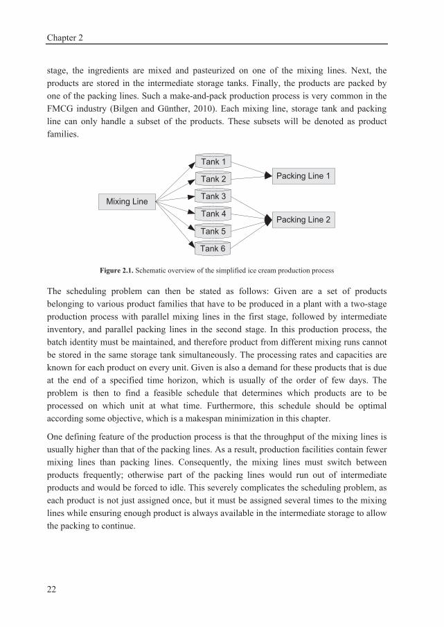
Chapter 2

22

stage, the ingredients are mixed and pasteurized on one of the mixing lines. Next, the products are stored in the intermediate storage tanks. Finally, the products are packed by one of the packing lines. Such a make-and-pack production process is very common in the FMCG industry (Bilgen and Günther, 2010). Each mixing line, storage tank and packing line can only handle a subset of the products. These subsets will be denoted as product families.

Figure 2.1. Schematic overview of the simplified ice cream production process

The scheduling problem can then be stated as follows: Given are a set of products belonging to various product families that have to be produced in a plant with a two-stage production process with parallel mixing lines in the first stage, followed by intermediate inventory, and parallel packing lines in the second stage. In this production process, the batch identity must be maintained, and therefore product from different mixing runs cannot be stored in the same storage tank simultaneously. The processing rates and capacities are known for each product on every unit. Given is also a demand for these products that is due at the end of a specified time horizon, which is usually of the order of few days. The problem is then to find a feasible schedule that determines which products are to be processed on which unit at what time. Furthermore, this schedule should be optimal according some objective, which is a makespan minimization in this chapter.

One defining feature of the production process is that the throughput of the mixing lines is usually higher than that of the packing lines. As a result, production facilities contain fewer mixing lines than packing lines. Consequently, the mixing lines must switch between products frequently; otherwise part of the packing lines would run out of intermediate products and would be forced to idle. This severely complicates the scheduling problem, as each product is not just assigned once, but it must be assigned several times to the mixing lines while ensuring enough product is always available in the intermediate storage to allow the packing to continue.

Scheduling

23

2.2.1. Additional Process Characteristics

The ice cream example contains several additional process characteristics that are found in many of the FMCG industry production processes. However, not all processes in the FMCG industry contain all characteristics. Since the objective is to develop a scheduling model suitable for the FMCG industry in general, the proposed model can handle scheduling problems with and without these additional process characteristics. In the model description in Section 2.5, the formulation will initially be based on a case study containing all the ice cream production process characteristics. However, alternative formulations for problems without each of these characteristics will also be given.

The first additional characteristic is that each production run must consist of a number of full storage tanks. In general, the industry policy is to use these full storage tank batches because it reduces waste production from changeovers and cleaning. In addition, it allows for fixed product recipe amounts which reduce the chance of human errors in the mixing process. If the full tank mixing run requirement is enforced, the batching decisions are fixed because each batch will consist of a single storage tank. Alternatively, without this requirement the batching decisions are included in the proposed model.

Secondly, the ice cream must be aged after the mixing and before the packing. Therefore, the ice cream mix must remain in the intermediate storage for a couple of hours. The length of the ageing time is product dependent. Thirdly, for hygienic reasons, the mixing line must be cleaned at least once every 72 hours. Other important characteristics are that each product is packed in a single continuous packing run, and that the changeover times are sequence-dependent.

2.3. Dedicated Time Intervals

Selecting the time representation is one of the key decisions in the development of a scheduling model (Floudas and Lin, 2004). A unit-specific continuous time interval approach, which is an approach that was originally developed by Ierapetritou and Floudas (1998), was selected for the proposed model. The main advantage of this approach is that it requires considerably fewer intervals than discrete time or global continuous time interval approaches. Those approaches mainly require more intervals because of the unaligned starting and ending times of the different stages, the varying batch production times, and the sequence-dependent changeovers.

As explained in the problem definition, the mixing lines switch frequently between products to prevent the packing lines from standing idle. As a result, the same product is almost never mixed in two consecutive mixing runs. This alternation can be exploited by introducing dedicated time intervals.

Chapter 2

24

A dedicated time interval is one in which only a certain product family can be produced. All products within a product family can be packed by the same packing lines and stored in the same intermediate storage tanks. Although it should be noted that these products cannot be stored in the same storage tanks simultaneously because the batch identity has to be maintained. For the example case study, two interval types are introduced: type 1 which is dedicated to the products for the first packing line and type 2 which is dedicated to the products that will be packed by the second packing line. This is shown in Figure 2.2, where for simplicity all intervals are of uniform length, and there is no time in between the intervals. However, in the proposed model the length of the intervals depends on the mixing and packing rates. In addition, there can be time in between intervals, either due to changeovers, or due to one of the lines standing idle.

Figure 2.2. Dedicated time interval overview.

However, pre-fixing product families to intervals could lead to suboptimal solutions since the pre-fixed ordering might not be the optimal ordering. Therefore, empty intervals are introduced. In each interval, either a product of the dedicated product family is produced, or no product is produced, and the interval is empty and has a zero length. In this way, the same product family can be produced in multiple consecutive intervals. Therefore, the ordering of product families is still flexible, and the optimal solution can be obtained.

Product family dedicated time intervals decrease the required computational time since the number of binary variables can be considerably reduced. For example, with two product families and a perfect alternation, the number of binary allocation variables can be reduced by 50%. However, since it should be possible to deviate from the pre-fixed ordering, a few extra intervals need to be added to the model to allow for the empty intervals. Therefore, the reduction in binary allocation variables is slightly less than 50%. It should be noted that a large number of empty intervals could even allow the model to obtain the optimal solution for a process without an alternating production of product families on the mixing lines. However, the formulation might be less efficient for such a process since it will require many empty intervals. An example of the use of dedicated time intervals to represent a not perfectly alternating production process is given in Figure 2.3.

Scheduling

25

Figure 2.3. Example of the Dedicated Time Intervals (DTI). From top to bottom: The defined horizon contains ten alternating dedicated time intervals. The optimal solution is not perfectly alternating. The dedicated time intervals can be used to represent the optimal solution with time intervals 2, 5 and 7 being empty intervals.

2.4. Inventory

One of the main issues associated with using a unit-specific continuous time approach for the ice cream scheduling problem is the modeling of the intermediate inventory. If the intermediate inventory is modeled in a straightforward manner, it would require its own intervals that need to be linked with the mixing and packing intervals. To reduce the computational impact of the intermediate inventory, an alternative method to model the intermediate inventory is used.

The model size is significantly reduced by not directly modeling the intermediate inventory. Instead the mixing intervals are coupled directly with the packing intervals. The start of a mixing interval is limited by the ending of previous packing intervals. This ensures that the mixing does not start before a tank is available to store the product. To be able to ‘count’ the number of storage tanks that are in use, at most one storage tank can be processed in each interval.

As an example, if two storage tanks can store product family 1, then the third mixing interval for product family 1 cannot start before the first packing interval has finished. This method can also be applied for multiple identical parallel lines since only one product per family can be processed per interval. More than two product families can be accommodated by introducing additional interval types.

2.5. Related Interval Method (RIM)

The constraints of the RIM are discussed in this section, and a schematic overview of the RIM is given in Figure 2.4. Some of the constraints of the model, most notably the timing and changeover detection constraints, are based on those from the MILP scheduling model from Erdirik-Dogan and Grossmann (2008). However, the introduction of dedicated time intervals and the new approach of dealing with the intermediate inventory require some modifications to these constraints.

Chapter 2

26

Figure 2.4. Schematic overview of the RIM model

2.5.1. Dedicated Time Intervals

The dedicated time intervals have been implemented into the RIM by introducing a repeating sequence of dedicated time intervals. Each sequence, denoted as repeating unit, contains the same number and ordering of dedicated time intervals. All product families must have at least one dedicated time interval in this repeating unit. However, if exactly one interval is used for each product family, the number of required empty intervals could be large if the average run length of some of the product families is longer than one interval.

Therefore, the number of intervals dedicated to each product family is based on the average mixing run length of that product family. If the average run length is unknown, half the number of available storage tanks for this product family can be used as an initial value. All intervals dedicated to the same product family in the repeating unit are ordered sequentially.

For the set-up in the example case study, the average mixing line run length for product family 1 is one tank, whereas the average run length for the product family 2 is two tanks. This difference is mainly because the storage tanks dedicated to family 1 are twice as large as those dedicated to family 2. In addition, four storage tanks can store product family 2, while only two can store family 1. Therefore, a repeating unit of one interval dedicated to product family 1 and two intervals dedicated to product family 2 is used. A schematic overview of the interval set-up is depicted in Figure 2.5.

Figure 2.5. A schematic overview of the dedicated time intervals used in the RIM model

The required number of intervals can be estimated based on the workload of both packing lines. First, the minimum number of repeating units can be estimated based on the demand. For example, if the total demand of product family 1 is six storage tanks, and if each repeating unit contains a single interval of type 1, then at least six repeating units are

Scheduling

27

required. In order to allow for empty intervals, this minimum number of repeating units is initially increased by 20%. If the obtained solution is not equal to the minimum makespan, which is explained in the result section, then this number can be increased by one repeating unit until no improvement in objective function is obtained.

2.5.2. Allocation

At most one product can be mixed during any time interval. Even if there are multiple mixing lines, only one of them can be assigned to each interval. This is necessary to be able to count the number of tanks that are currently in use. Clearly, multiple mixing lines can be active simultaneously, which is achieved by allowing intervals on different mixing lines to overlap. Most of the variables and constraints are only declared for those intervals in which a certain product family can be processed according to the dedicated time intervals. The domain over which each variable is declared is given in the nomenclature.

,

1 i,m,ti m

WM t (2.1)

The packing and mixing intervals are related directly. That is to say, if product i is mixed in interval t, then product i will also be packed in interval t. Later, the start times of these intervals will be related to ensure that the product is aged before the packing starts. In the following constraint, an inequality is used because of the empty intervals. For the mixing lines, the binary allocation variables can be zero since the changeovers are based on WMdummy. However, calculating the changeovers for the packing lines and ensuring single continuous packing runs is facilitated by having a product assigned to every interval. It should be noted that WP must be treated as a binary variable if there is more than one packing line per family. If there is only one packing line per family, WP can be relaxed as a continuous variable.

i,p,t i,m,t tp m

WP WM i IT ,t (2.2)

2.5.3. Production Amounts

Each mixing run must consist of a number of full tanks. Each interval consists of the production of exactly one storage tank. If mixing runs are not restricted to full tanks, constraint (2.3) can be written as an inequality. In that case, the model would solve both the batching and scheduling problems simultaneously.

, , , , i m t i m t i tPM WM STC i IT ,m,t (2.3)

Chapter 2

28

The total production of product i is less than or equal to the demand. Alternatively, the demand could be used as a lower bound when either maximizing the total production or minimizing the makespan.

, ,,

i m t im t

PM D i (2.4)

The amount packed in a packing interval must be equal to the amount mixed in the corresponding mixing interval since the mixing and packing intervals are coupled.

i,p,t i,m,t tp m

PP PM i IT ,t (2.5)

In addition, a packing line must be assigned to a product to be able to pack that product.

, , , ,i,p,t i i p t p tPP STC WP i IP IT p t (2.6)

2.5.4. Empty Intervals

An interval is empty when no product is assigned to the mixing line m in interval t.

, , , 1 i m t m ti

WM WEI m,t (2.7)

At most two out of three consecutive intervals are allowed to be empty intervals on all mixing lines. Having three empty intervals in a row would serve no real purpose as these intervals could simply be removed from the model. The NM parameter is the number of mixing lines. An interval will always be empty on at least NM-1 lines since at most one mixing line can be assigned in each interval. The total number of empty lines per three consecutive intervals must thus not be more than 3(NM-1)+2.

2

, 3 -1 +2 t

m t'm t' t

WEI NM t (2.8)

The inventory is considered by counting the number of tanks that have been mixed but that have not yet been packed. However, empty intervals should not be considered when counting the intervals. WEI2t,t’ is used to determine whether at least two intervals are empty on all mixing lines in a set of intervals. Only intervals dedicated to the same product family are included in this range since the other products are stored in different storage tanks. The number of intervals in this range is the number of storage tanks dedicated to this product family plus 1. The Nfn,t parameter indicates the number of intervals that should be moved forward until the nth interval dedicated to the same family. In this way, the number of

Scheduling

29

intervals dedicated to a product family in an interval range can be related to the total number of intervals in this range.

If the first interval in this range is not empty on all mixing lines, this variable is set to zero. There could still be two completely empty intervals in the range of intervals, but this will then be covered by one of the subsequent WEI2t,t’ variables. Subtracting NM-1 from

,m tm

WEI gives 1 if the interval is empty on all mixing lines and 0 if one of them is active.

, , , ,1 , , | cc t t' m t c c n NST t

mWEI2 WEI NM c t TC t' TC t t' t Nf (2.9)

WEI2t,t’ is set to zero if none of the intervals after t and before t’+1 are empty on all mixing lines. Only those intervals in which the same product family as in interval t is mixed are included. To ensure that only intervals that are empty on all mixing lines are counted, the NM-1 is again subtracted from each ,m t

mWEI in the summation.

'

, , ,1

,

1

, , ' , ' 'c

c

t

c t t' m t''t'' TC t m

c c n NST t

WEI2 WEI NM

c t TC t TC t t t Nf (2.10)

2.5.5. Mixing Line Changeovers

To facilitate the modeling of changeover constraints, the variable WMdummyi,m,t is introduced. In principle this variable is equal to the true assignment variable WMi,m,t. However, with the additional requirement that exactly one product is assigned to each interval. This ensures that, even when empty intervals in WMi,m,t are allowed, only changeovers between consecutive intervals have to be considered. The product assignment in empty intervals will be equal to the assignment in the interval before or after since the changeover time between two batches of the same product is zero.

, , , , , ,i m t i m t tWMdummy WM i IT m t (2.11)

, , 1 ,i m ti

WMdummy m t (2.12)

If product i is mixed in interval t, then there is exactly one changeover from this product i to any other product. The following constraint forces the changeover variable to one if WM is one since all changeover variables are 0-1 continuous variables.

i,i',m,t i,m,ti'

WMCO WMdummy i,m,t NT (2.13)

Chapter 2

30

Similarly, if product i’ is mixed in interval t+1, then there is exactly one changeover from any product to this product i’.

1 i,i',m,t i',m,t+i

WMCO WMdummy i',m,t NT (2.14)

Finally, each interval has exactly one changeover:

i,i',m,ti,i'

WMCO = 1 m,t (2.15)

2.5.6. Mixing Times

The end time of mixing interval t is equal to the starting time of this interval, plus the time required to mix the product in this interval.

, ,, , ,i m t

m t m ti i

PMTEM TSM m t

PRM (2.16)

Intervals of the same product family on different mixing lines should be in the correct order. By enforcing this, the number of intervals can be counted to determine how many storage tanks of a product family are in use. However, only the nonempty intervals are required to be in the correct order. As a result, intervals of different product families on different mixing lines are allowed to be in any order.

, , , , | m t m',t' m t m t' c cTSM TSM H WEI WEI c m,m',t TC ,t' TC t t' (2.17)

All intervals must end before the end of the time horizon.

, ,m tTEM H m t NT (2.18)

Mixing interval t cannot start before the end of the previous interval plus the changeover time from interval t-1 to t.

1 1 , m,t i,i',m,t i,i' m ti,i'

TEM WMCO COTM TSM m,t (2.19)

2.5.7. Packing Changeovers

The product assignment of the empty packing intervals is set equal to the assignment in the previous interval dedicated to the same product family. This is possible since each product is packed in a single continuous campaign without changeovers. For a packing interval to be empty, this mixing interval must be empty on all mixing lines.

Scheduling

31

, ,

1 1 , 1n t n ti,p,t m,t+Nf i,p,t Nf p t

mWP + WEI NM WP i IP IT , p,t n (2.20)

If product i is packed in interval t, then there must be a changeover from this product to any other product after this interval.

i,i', p,t i,p,t p ti'

WPCO WP i IP IT , p,t NT (2.21)

If product i’ is packed in interval t+Nfn,t, then there must be a changeover from any product to this product i’ after interval t. The interval t+Nfn,t with n=1 is the first interval after the current interval that is dedicated to the same product family.

,' ' ' , 1

n ti,i ,p,t i ,p,t+Nf p ti

WPCO WP i IP IT , p,t n (2.22)

Each interval has exactly one changeover on each packing line that can pack the product family to which the interval is dedicated.

1 i,i', p,t ti,i'

WPCO p PT ,t (2.23)

2.5.8. Packing Times

The end of each packing interval is equal to the start time plus the time required to pack the product in that interval.

i,p,tp,t p,t t

i i

PPTEP = TSP + p PT ,t

PRP (2.24)

All packing intervals must end before the end of the time horizon.

p,t tTEP H p PT ,t (2.25)

Each product is packed in a single continuous packing campaign. Therefore, the time between packing intervals is zero when the same product is produced in both intervals. Since the changeover time from a product to the same product is zero, the changeover variable is multiplied by the changeover time to limit the time between intervals. The changeover time is multiplied by a big-M parameter to ensure the time between intervals can take any value for nonzero changeovers. For the examples in this chapter the big-M parameter was set to 25.

, '

p,t i,i', p,t i,i' ti i

TBP M WPCO COTP p PT ,t (2.26)

Chapter 2

32

The next interval starts at the end time of the previous interval, plus the changeover time, plus the time between packing intervals. The following constraint, together with constraint (2.26), ensures that there is no delay between the packing of the same product in subsequent intervals.

,, '

, , , 1 |

n tp,t i,i',p,t i i p,t p,t Nfi,i'

t c

TEP WPCO COTP TBP TSP

c p PT t TC n t NT (2.27)

2.5.9. Intermediate Inventory

The inventory restrictions are enforced by counting the number of tanks that are currently in use. Since the mixing and packing intervals are coupled, the packing of the nth interval of a product family must finish before the mixing of the NSTc+nth interval of the associated type can start, with NSTc being the number of tanks that are available to store this product family. However, when one of these intervals is an empty interval, this constraint is relaxed. The time horizon is used as the big-M parameter. The t-Nbn,t gives the interval that is the nth previous interval dedicated to the same product family as interval t.

,,

' '' '

1

, , , ,

n tc n t

t

p,t -Nb m,t m ,tt TC t Nb m

t c c

TEP TSM M WEI NM

c m p PT t TC n NST

(2.28)

If the previous constraint is relaxed, then the NSTi+n+1th interval of this type cannot start mixing before the nth interval has finished packing. If this stretch of intervals contains two or more empty intervals, this constraint is relaxed.

,,

1

, ' ''' '' ' 1

, , , 1

n tc n t c

t t

p,t -Nb m,t c t ,tt TC t Nb t TC t

t t c

TEP TSM M WEI2

c m p PT ,t TC n NST

(2.29)

If the previous constraint is relaxed due to two empty intervals, then the NSTi+n+2nd interval of the same type cannot start mixing before the nth interval has finished packing. In theory, this stretch could contain three or more empty intervals, in which case the constraint could be relaxed again. However, in general, when using a high utilization percentage the products are packed well before the NSTi+n+2nd interval. Therefore, no relaxation conditions are added to the following constraint, but the model can easily be modified when this relaxation is required.

,

, , , 2n tp,t -Nb m,t t c cTEP TSM c m p PT ,t TC n NST (2.30)

Scheduling

33

2.5.10. Ageing Times

A batch cannot be packed before the end of the mixing plus the ageing time. The constraint is relaxed for empty intervals.

, ,p,t m,t i i,m,t m t ti

TSP TEM AgeT WM H WEI m p PT ,t (2.31)

2.5.11. Periodic Cleaning Intervals in the Mixing Line

Two different methods could be used to deal with the cleaning time. The first one is specific to the example problem and will be discussed below. The second method is more general, though less efficient for the example problem, and it is discussed in Appendix A.

At least one cleaning interval is required because the horizon is 120 hours, and a cleaning interval is required once every 72 hours. Since the objective is to maximize production or minimize makespan, the minimum number of cleaning intervals will lead to the maximum production. As a result, exactly one cleaning interval is required for the example problem. The binary variable WCIm,t is introduced, which is one if a cleaning interval precedes the current interval. The first constraint ensures that each mixing line has exactly one cleaning interval.

, 1 m tt

WCI m (2.32)

For this cleaning interval, at least 4 hours are required between the end of the previous interval and the start of the next interval:

, ,, 1 4 ,m t m tm tTSM TEM WCI m t (2.33)

Also, this cleaning interval must not be later than 72 hours after the start or earlier than 72 hours before the end of the last mixing interval because then two cleaning intervals would be required. These 72 hours (CIfrequency) are the minimum cleaning interval frequency.

, , ,1 , ,m t' m t m tTEM CIfrequency H WCI TSM m t t' NT (2.34)

, ,1 ,m t m tTSM CIfrequency H CIfrequency WCI m t (2.35)

2.5.12. Single Campaign per Product

A production campaign is started only once for each product.

Chapter 2

34

, ,,

1 i p tp t

WPstart i (2.36)

If product i is packed in interval t and is not packed in the previous interval dedicated to this product family, then interval t is the start of a production campaign for product t.

, , , 1

n ti,p,t i,p,t i,p,t -Nb p tWPstart WP -WP i IP IT p,t n (2.37)

2.5.13. Symmetry Breaking

If multiple intervals are dedicated to a single product family in the repeating unit, the number of equivalent solutions can be reduced by enforcing that a product can only be mixed in the second of these intervals if one is mixed in the first as well.

, ' | '= 1i,m,t i,m,t' c ci i

WM WM c m,t TC ,t TC t t (2.38)

2.5.14. Objective Function

Two different objective functions are used in this chapter. The first option is maximizing the production, while having the demand as an upper bound. This has been defined as the feasibility objective function, as the optimization attempts to find a feasible schedule where the demand is met. In this case, the following objective is used.

, ,, ,

i p ti p t

obj PP (2.39)

The second objective function is a makespan minimization. Constraint (2.4) is replaced by constraint (2.40). The objective function is given in constraint (2.41):

, , i m t im t

PM D i (2.40)

obj MS (2.41)

The makespan is defined by the following constraint. Only the packing end time is considered since the packing will always end after the mixing.

, ,p tMS TEP p t (2.42)

Scheduling

35

2.5.15. Additional Process Characteristics

The formulation discussed in this chapter includes all additional process characteristics mentioned in Section 2.2.1. However, the RIM can also be used for problems without these additional process characteristics. In this section, the alternative formulation for problems without some of these additional process characteristics will be given. The first characteristic is the requirement of full tank mixing runs. The model can consider non-full tank mixing runs by substituting constraint (2.3) with the following inequality:

, , , , i m t i m t i tPM WM STC i IT ,m,t (2.43)

Secondly, for a product without an ageing time requirement, the ageing time term can be removed from constraint (2.31). Thirdly, constraints (2.32)-(2.35) can be removed if there is no periodic cleaning requirement. Without the requirement for a single continuous packing campaign, constraints (2.26), (2.36) and (2.37) can be removed, and constraint (2.27) can be substituted with constraint (2.44).

,

, , 1 |

n tp,t i,i',p,t i,i' p,t Nfi,i'

t c c

TEP WPCO COTP TSP

c p PT ,t TC n t LastDTI (2.44)

Finally, in the ice cream case study each product family can only be stored in storage tanks of equal size. The model can deal with various storage tank sizes for a single product family by introducing a dedicated time interval type for each storage tank size. In this case, the storage tank capacity STCi,t no longer just depends on the product but also on the interval. Also, the last interval of a type, LastDTIc, refers to the last interval dedicated to a product family and, therefore it is the same for storage tank types that can store the same product family. In addition, the Nfn,t and Nbn,t parameters in the inventory constraints (2.28)-(2.30) should be replaced by similar parameters based on the number of intervals until the nth next/previous interval dedicated to the same storage tank type. The other constraints still require the original Nbn,t and Nfn,t to be based on the number of time intervals until the next/previous interval dedicated to the same product family.

2.6. STN Model

To evaluate the efficiency of the developed problem-specific model, it will be compared to the unit-specific event-based continuous time STN model by Shaik and Floudas (2007). An STN formulation was selected as such a formulation is capable of dealing with a wide range of process characteristics. Shaik and Floudas (2007) compare their model to several other models using case studies with various inventory limitations. Their model could always obtain the global optimal solution and, on average, it was the most efficient formulation.

Chapter 2

36

Therefore, their model was selected to be compared with the developed model and to evaluate the impact of dedicated time intervals. Several constraints of their model have to be modified since the process they describe differs from the ice cream production process. The modified model is given in Appendix B.

The two differences between the STN and the developed problem-specific model that are expected to have the largest computational impact are the introduction of dedicated time intervals and the different ways of modeling the intermediate storage. To estimate the impact of the dedicated time intervals, the model presented in this chapter is also compared to a version of the STN that uses dedicated time intervals. This is the regular STN model with an additional constraint that forces the binary assignment variables to zero for those task/event combinations where the event is not dedicated to the product family processed in the task.

2.7. Results

First, four small example case studies are used to compare the computational efficiency of the RIM with the STN. Subsequently, the RIM is compared to the models of Subbiah et al. (2011) and Kopanos et al. (2011a) using 10 full scale example case studies without periodic cleaning. In the final part of this section, the RIM is used to optimize the same 10 case studies with periodic cleaning.

All case studies are based on the ice cream scheduling case study introduced by Bongers and Bakker (2006). The plant consists of one mixing line, six storage tanks and two packing lines, and it processes two product families. The connectivity between the equipment is shown in Figure 2.1. Both product families can be mixed by the same mixing line. Products of the first product family can be handled by the first two storage tanks and the first packing line. Products of the second product family can be handled by storage tanks 3-6 and the second packing line.

The mixing rate for all products is 4500 kg/hr, the storage capacity of tanks 1-2 is 8000 kg, and the storage capacity of tanks 3-6 is 4000 kg. Table 2.1 lists the packing rates and the ageing time for all the products. Note that products 1-4 correspond to product family 1, while products 5-8 correspond to product family 2.

Table 2.2 lists the required changeover times for the packing lines. For example, the required changeover time from product P2 to product P3 on a packing line is 60 minutes. Table 2.3 lists the required changeover times on the mixing line. The data in Table 2.1-2.3 is identical for all case studies that were studied, although the small case studies did not contain all eight products. All optimizations were performed using Gurobi 3.0 in AIMMS 3.10 on a computer with an Intel(R) Core(TM)2 Duo CPU P8700 2.53 GHz and with 4 GB of memory.

Scheduling

37

Table 2.1. Packing rates and ageing times Packing Rate [kg/hr]

Product Line 1 Line 2 Ageing Time P1 1750 - 1 hr P2 1500 - 3 hr P3 1000 - 3 hr P4 1500 - 0 hr P5 - 1750 2 hr P6 - 2000 2 hr P7 - 2000 2 hr P8 - 2000 2 hr

Table 2.2. Packing line changeover times [min] between products P1-P8 P1 P2 P3 P4 P5 P6 P7 P8

P1 60 60 60 - - - - P2 30 60 60 - - - - P3 30 30 60 - - - - P4 30 30 30 - - - - P5 - - - - 60 60 60 P6 - - - - 30 60 60 P7 - - - - 30 30 60 P8 - - - - 30 30 30

Table 2.3. Mixing line changeover times [min] between products P1-P8 P1 P2 P3 P4 P5 P6 P7 P8

P1 30 30 30 30 30 30 30 P2 30 30 30 30 30 30 30 P3 30 30 30 30 30 30 30 P4 30 30 30 30 30 30 30 P5 30 30 30 30 15 15 15 P6 30 30 30 30 5 15 15 P7 30 30 30 30 5 5 15 P8 30 30 30 30 5 5 5

2.7.1. Small Example Problems

The four small example problems are based on a 48 hour horizon. The cleaning interval frequency is every 36 hours, and the cleaning interval duration is 2 hours. The demands are listed in Table 2.4. In case study A the first packing line is the bottleneck, in case study B the second packing line is the bottleneck, in case study C the workload on both lines is similar, and case study D considers different products.

Chapter 2

38

Table 2.4. Demand [kg] Case Study A B C D Product 1 40,000 40,000 32,000 - Product 2 24,000 16,000 32,000 16,000 Product 3 - - - 16,000 Product 4 - - - 16,000 Product 5 40,000 40,000 48,000 - Product 6 24,000 28,000 20,000 - Product 7 - - - 40,000 Product 8 - - - 32,000

The feasibility objective was used for all four case studies. This objective function is explained in Section 2.5.14. The computational results are given in Table 2.5. STN* is the STN model using dedicated intervals. For the RIM and the STN*, the number of time intervals is equal to the initial estimate explained in Section 2.5.1. For the STN, the number of intervals is equal to the number of batches since it does not contain any empty intervals.

Table 2.5. Computational results of case studies A-D Case Study

Model Intervals /Events

Variables (Binary)

Constraints Required CPU Time

Objective

A RIM 30 1319(90) 1600 1s 128,000 STN 24 1946(504) 13699 521s 128,000 STN* 30 2432(630) 20366 51s 128,000

B RIM 30 1319(90) 1600 1s 124,000 STN 24 1946(504) 13699 600s 124,000 STN* 30 2432(630) 20366 24s 124,000

C RIM 30 1319(90) 1600 11s 132,000 STN 25 2027(525) 14720 837s 132,000 STN* 30 2432(630) 20366 322s 132,000

D RIM 33 1892(110) 1928 1s 120,000 STN 24 2330(600) 21460 2293s 120,000 STN* 33 3203(825) 38570 405s 120,000

By comparing the different model sizes, it can be seen clearly that the alternative method of modeling the intermediate inventory results in considerably smaller models. In particular, the number of constraints is reduced by one order of magnitude. Even though the STN requires the fewest intervals, the RIM contains far fewer binary variables since it only requires binary mixing line allocation variables and a binary cleaning interval variable. The number of binary variables in the STN* is larger than in the STN model because it requires more intervals. However, half of the binary allocation variables are forced to zero because the product processed in a task is not part of the dedicated product family.

Scheduling

39

For all models feasible schedules for the 4 small example case studies could be obtained. As is clear from Table 2.5, the regular STN model is computationally the most expensive for these case studies. This was expected, as the STN* and RIM are more specific and exploit the features of this problem, whereas the STN model is intended to solve more general problems. While the STN* model with dedicated time intervals is more efficient than the regular STN, it is still far less efficient than the RIM. From this it may be concluded that both the alternative method of modeling the intermediate inventory and the dedicated time intervals result in more efficient models.

2.7.2. Full Scale Example Problems without Periodic Cleaning

In this section, the RIM will be compared with models by Subbiah et al. (2011) and Kopanos et al. (2011a) that are also used to optimize the ice cream scheduling process. However, before the computational comparison, the differences in the ice cream production processes considered in the various papers will be discussed. First, Subbiah et al. (2011) and Kopanos et al. (2011a) do not consider the periodic cleaning of the mixing line. This periodic cleaning severely complicates the scheduling as the freedom on the non-bottleneck mixing and packing lines is reduced. Therefore, a version of the RIM without periodic cleaning will be compared with their models.

Secondly, the inventory requirements are relaxed in the model of Subbiah et al. (2011). They implicitly assume that the intermediate storage is only required between the end of the mixing and the start of the packing. As a result, the schedule they obtain would be infeasible for the production process discussed in this chapter as it violates the maximum available inventory.

Except for the periodic cleaning, the production process considered by Kopanos et al. (2011a) is the same as in this chapter. However, it should be noted that their precedence based model has a limited flexibility regarding certain process characteristics. For example, it requires that the batching decisions must be made before the scheduling. This may lead to suboptimal solutions if full mixing runs are not required. Similarly, their model may also lead to suboptimal solutions when a product can be stored in storage tanks of different sizes. In addition, the efficiency of their formulation could be significantly reduced without the single continuous packing campaigns requirement. The efficiency would be reduced because the tightening constraint linking the ordering of batches on a mixing line to the ordering of products on a packing line could no longer be used.

The models are compared based on full scale case studies over a 120 hour horizon. The demand for the full scale example case studies is given in Table 2.6. The RIM is first compared with the model of Subbiah et al. (2011) based on the first example and subsequently with the model of Kopanos et al. (2011a) based on all 10 examples. It should

Chapter 2

40

be noted that example 1 was first introduced by Bongers and Bakker (2006) and examples 2-10 by Kopanos et al. (2011a).

Table 2.6. Demand [kg] of products P1-P8 for case studies 1-10 Case Study

P1 P2 P3 P4 P5 P6 P7 P8

1 80,000 48,000 32,000 8,000 112,000 12,000 48,000 24,000 2 48,000 56,000 16,000 48,000 80,000 44,000 12,000 64,000 3 32,000 32,000 40,000 32,000 32,000 60,000 44,000 80,000 4 8,000 32,000 64,000 24,000 52,000 44,000 88,000 32,000 5 88,000 16,000 24,000 40,000 12,000 48,000 64,000 84,000 6 16,000 16,000 16,000 88,000 24,000 24,000 104,000 52,000 7 8,000 8,000 96,000 8,000 116,000 64,000 4,000 4,000 8 16,000 40,000 32,000 56,000 36,000 40,000 60,000 60,000 9 48,000 24,000 56,000 16,000 8,000 92,000 20,000 88,000 10 8,000 72,000 8,000 72,000 80,000 80,000 4,000 32,000

In these case studies without periodic cleaning, the freedom on the non-bottleneck stage increases significantly, and therefore the RIM requires fewer empty intervals. Hence, for the case studies without periodic cleaning, the number of intervals is set equal to the minimum number of repeating units plus 10%. This is sufficient to obtain the global optimal solution for all 10 case studies. Overlapping decisions from the previous week are not considered.

Similarly to Subbiah et al. (2011) and Kopanos et al. (2011a), a heuristic is used to predefine the sequence of products on the packing lines. This heuristic is also similar to the partial pre-ordering of Jain and Grossmann (2000). The ordering applied on each packing line is the ordering for which the makespan would be minimal if the capacities of all other stages are neglected. This makespan is denoted as the theoretical minimum makespan.

For the bottleneck stage, the ordering leading to the theoretical minimum makespan is most likely the optimal ordering, since any other ordering would lead to an overall makespan larger than the theoretical minimum makespan. However, the interaction between the tasks may lead to a makespan larger than the theoretical minimum makespan (Raaymakers and Fransoo, 2000). The interaction between the tasks may especially increase the makespan if the flexibility is decreased by enforcing the minimum makespan ordering on all lines. Therefore, the optimal ordering on the non-bottleneck stages is not necessarily equal to the theoretical minimum makespan ordering since the non-bottleneck stages contain some slack. If the obtained solution has a higher makespan than the theoretical minimum makespan, the ordering on the non-bottleneck stages could be removed. However, for all case studies without periodic cleaning, the global optimal solution could be obtained while enforcing the ordering on all packing stages.

Scheduling

41

For the first packing line, the optimal ordering is 4-3-2-1 since that sequence minimizes both the changeover times and the ageing time of the first product. When using this ordering, the theoretical minimum makespan is equal to the active packing time (115.05 hours), plus the mixing time of the first batch of product 4 (1.78 hours), plus the ageing time of product 4 (0 hours), plus the packing changeover times (3 0.5 hours). The total theoretical minimum makespan is thus 118.33 hours. The second best ordering would require at least half an hour more in changeover time. For the second packing line, the optimal ordering is 8-7-6-5 with a theoretical minimum makespan of 110.39. For the second packing line, a different ordering would increase the makespan by at least half an hour as well. The theoretical minimum makespan of the packing stages can be used as a lower bound in the makespan minimization. This lower bound is added to the model in a tightening constraint similar to constraint 18 in Kopanos et al. (2011a).

Theoretical Minimum MS pMS p (2.45)

The ordering heuristics are implemented as constraints. For example, the following constraint enforces the 4-3-2-1 and 8-7-6-5 ordering. A different ordering could be used by changing the domain of c, i and i’.

, , ', ,

, ' , | '

i p t i p tt t

p c p c

t WPstart t WPstart

c i IP IC ,i IP IC p i i (2.46)

Additionally, part of the binary allocation variables can be forced to zero when the products are ordered. For example, if product 4 is mixed first, the first few intervals of type 1 cannot produce any other product than product 4. The length of this interval range is equal to the number of storage tanks of product 4 that must be mixed. In more general terms, the first X intervals of type c cannot mix product i, where X is equal to the minimum number of intervals that are required to mix the products that precede product i in the ordering. For the 4-3-2-1 and 8-7-6-5 ordering the constraint is the following. A constraint with different domains of c, i and i’ can be used to implement any ordering of products.

'

, ,, '

0 , , , , ' | i

ii IT it

i m t t c c Dn t

STC

WM c i IT m t TC t FirstDTI t Nf (2.47)

Similarly, the last Y intervals of type c cannot mix product i, where Y is equal to the minimum number of intervals that are required to mix the products that follow product i in the ordering. For the 4-3-2-1 and 8-7-6-5 ordering the constraint is the following. A constraint with different domains of c, i and i’ can be used to implement any ordering of products.

Chapter 2

42

' <

, ,, '

0 , , , , ' | i

ii IT it

i m t t c c DN t

STC

WM c i IT m t TC t LastDTI t NT Nb (2.48)

The RIM model for case study 1 without periodic cleaning contains 81 intervals and is composed of 6,443 constraints, 9,169 continuous variables and 324 binary variables. The RIM requires 12s to obtain the global optimal solution for case study 1. The solution is the global optimal solution since the makespan of 118.33 hours is equal to the theoretical minimum makespan. The resulting Gantt chart is given in Figure 2.6.

Figure 2.6. Gantt chart of the optimal schedule for case study 1 without periodic cleaning

The model of Subbiah et al. (2011) requires a similar computational effort of 15s to obtain a solution. However, this solution is not the global optimal solution. The makespan of their solution is 0.67 hr longer than the optimal solution. Moreover, their model relaxes the inventory requirements as it only requires intermediate inventory between the end of the mixing and the start of the packing. As a result, the schedule they obtain would not be feasible for the ice cream production process described in this chapter.

The computational results of the RIM for all 10 case studies are summarized in Table 2.7. It should be noted that the makespan does not include a two hour cleaning interval at the end of the horizon on all mixing and packing lines. Since this cleaning interval is added at the end of the last activity on each line, and since it is the same length for all lines, this cleaning interval does not influence the decisions in a makespan minimization. The optimal solution was obtained for all 10 case studies, and the required computational time ranged from 12s to 170s. Kopanos et al. (2011a) report required computational times between 1s to 51s to obtain the optimal solution. It should be noted that these CPU times are not directly comparable because Kopanos et al. (2011a) used a different computer, modeling software and solver.

Nevertheless, the model of Kopanos et al. (2011a) seems computationally slightly more efficient, although both models are able to obtain the global optimal solution of all example case studies within minutes of CPU time. On the other hand, the RIM is more flexible to the process characteristics. In order to demonstrate this flexibility, the RIM is used to optimize the first five full scale example case studies with various process characteristics. These case studies are optimized without the single continuous packing campaign requirement, without the full tank mixing runs requirement, without the ageing time requirement and with different storage tank sizes. For this last scenario, the available storage capacity is changed

Scheduling

43

for product family 2 to two tanks of 4000kg and two tanks of 6000kg. The required modifications to the RIM for these case studies are discussed in Section 2.5.15.

Table 2.7. Computational results of the RIM for the full scale case studies without periodic cleaning Case Study

Intervals Constraints Continuous Variables

Binary Variables

MS [hr] CPU Time[s]

Case 1 81 6,443 9,493 324 118.33 12 Case 2 84 6,677 9,845 336 116.04 95 Case 3 90 7,139 10,549 360 114.67 54 Case 4 90 7,136 10,549 360 116.10 124 Case 5 87 6,914 10,197 348 114.90 155 Case 6 84 6,668 9,845 336 108.10 121 Case 7 78 6,188 9,141 312 114.52 59 Case 8 81 6,434 9,493 324 108.42 86 Case 9 87 6,905 10,197 348 113.37 170 Case 10 81 6,440 9,493 324 111.85 153

Table 2.8. Required computational time and makespan of the RIM for variations of the first 5 full scale example case studies

Case Study

No Single Packing

Campaign

Non Full Tank Mixing Runs

No Ageing Time Different Storage Tank

Capacities CPU Time

[s]

MS [hr]

CPU Time

[s]

MS [hr]

CPU Time

[s]

MS [hr]

CPU Time

[s]

MS [hr]

1 81 118.33 69 118.33 13 118.33 86 118.33 2 160 116.04 64 116.04 15 116.04 98 116.04 3 23 114.67 25 114.67 11 112.67 171 114.67 4 135 116.10 33 116.10 19 114.10 317 116.10 5 201 114.90 33 114.90 19 114.90 167 114.90

As can be seen from Table 2.8, the RIM is also computationally efficient for these case studies. In fact, without the full tank mixing runs requirement, and especially without the ageing time requirement, the required computational effort decreases. On the other hand, with storage tanks of different sizes the complexity of the problem seems to increase slightly. The required computational time also increases slightly without the single continuous packing campaign requirement. Solutions with a makespan equal to the theoretical minimum makespan were obtained for all case studies in the reported computational time. It should be noted that without the ageing time requirement, the theoretical minimum makespan of case studies 3 and 4 decreases by 2 hours.

Chapter 2

44

2.7.3. Full Scale Example Problems with Periodic Cleaning

The RIM was selected for the optimization of the example case studies with periodic cleaning because of the flexibility and because the RIM is also able to obtain optimal solutions within minutes. These case studies are the same example problems as discussed in the previous section. However, a 4 hour cleaning interval is now required once every 72 hours. The number of intervals is set to 20% more than the minimum number of repeating units as was explained in Section 2.5.1. The RIM model for the first case study contains 87 intervals and is composed of 7,028 constraints and 10,156 variables, of which 435 are binary. For this first case study, the RIM model is able to find the optimal schedule with a makespan of 118.33 hour in 2074s.

2.7.3.1. Algorithm Outline

An algorithm was developed to reduce the required CPU time. This algorithm will first be introduced, then demonstrated on case study 1, and finally the results for the other 9 case studies will be given as well. The outline of the algorithm is as follows:

Step 1: Identify the bottleneck stage by calculating the theoretical minimum makespan of all stages

Step 2: Order the products according to the theoretical minimum makespan for each packing stage

Step 3: Relax the horizon by 1%, and perform a makespan minimization with large optimality tolerance to obtain an initial solution.

Step 4: Fix the allocation decisions in the first 1/3rd of the schedule, and perform a makespan minimization. If the obtained makespan is equal to the theoretical minimum makespan, terminate the algorithm.

Step 5: Fix the allocation decisions in the last 1/3rd of the schedule, and perform a makespan minimization. If the obtained makespan is equal to the theoretical minimum makespan, terminate the algorithm.

Step 6: Fix the bottleneck stage allocation decisions, and perform a makespan minimization. If the obtained makespan is equal to the theoretical minimum makespan, terminate the algorithm. Otherwise, go to step 4.

After Steps 4-6: If the makespan in three consecutive steps is identical, remove the ordering on the non-bottleneck packing stage with the lowest theoretical minimum makespan. If the ordering on all non-bottleneck packing stages was already removed, terminate the algorithm.

Scheduling

45

In step 3 the horizon is slightly relaxed to obtain an initial solution faster. This solution does not necessarily have to be feasible since the other steps in the algorithm will improve the solution. A sufficient optimality tolerance is used in this step such that the optimization terminates at the first solution that is feasible for the relaxed horizon.

If an identical solution is obtained in steps 4-6, the ordering on one of the non-bottleneck stages is removed. This is necessary since the ordering on the non-bottleneck stages is not necessarily equal to the minimum makespan ordering on this non-bottleneck stage. The reason is that this packing line contains some slack when compared to the bottleneck packing line. Therefore, using a different order, with for example longer changeovers, will not necessarily lead to a longer overall makespan.

In fact, the interaction between the mixing and packing stages is such that the optimal order on the non-bottleneck packing lines may be dictated by the order on the bottleneck packing line. For example, the allocation on the non-bottleneck packing line could be such that the cleaning interval on the mixing line does not affect the bottleneck packing line. As a result, the non-bottleneck packing line might be standing idle for a brief period and have slightly longer changeovers, but since there is some slack the total makespan would not necessarily increase. A time limit of 15 minutes is used in steps 4-6 since typically the global optimal solution could be obtained faster by switching between steps than by continuing to optimize a single step until optimality is proven for that step.

2.7.3.2. Algorithm Example

Next, the algorithm is applied to the first full scale example case study. In the first two steps, the horizon is relaxed by 1% to 121.2 hours, and a 4-3-2-1 ordering on packing line 1 and an 8-7-6-5 ordering on packing line 2 is enforced. By relaxing the time horizon, the capacity utilization is decreased, which makes it considerably easier to obtain a schedule. After 191s the schedule shown in Figure 2.7a with a makespan of 121.10 hours was found. While this initial schedule is infeasible as the production time is longer than 120 hours, it can be used as a starting point for the algorithm.

In the other steps of the algorithm, makespan minimizations will be performed while part of the schedule is fixed. First, in step 4 all allocation decisions in the first 1/3rd of the schedule are fixed. In this case study, the allocation decisions in the first 28 intervals are fixed. After 72 seconds the schedule shown in Figure 2.7b with a makespan of 119.16 hours was obtained. In step 5 the allocation in the last 28 intervals is fixed. After 418s the schedule shown in Figure 2.7c with a makespan of 118.33 hours was found. The algorithm was terminated because 118.33 hours was equal to the theoretical minimum makespan. The total required computational time by the algorithm was 681s which is considerably shorter than the 2074s required for the one step full space optimization.

Chapter 2

46

Figure 2.7. Gantt chart of the full scale problem after step 3 (a), step 4 (b) and step 5 (c) of the algorithm

2.7.3.3. Algorithm Results

The algorithm was also applied to the other 9 example case studies used in Kopanos et al. (2011a) with the addition of the periodic cleaning requirement on the mixing lines, which is not handled by their model. The computational results for all 10 case studies are summarized in Tables 2.9-2.11. For all case studies except for case study 10, the algorithm was able to find a solution with a makespan equal to the theoretical minimum makespan. Therefore, for case studies 1-9 the algorithm was able to find the global optimal solution. For case study 10 the theoretical minimum makespan is 111.85. The obtained solution is thus within 0.7 hour, or 0.6%, of the lower bound.

Table 2.9. Computational results of the algorithm. Required computational time and makespan for the full scale case studies 1-4.

Case Study 1 Case Study 2 Case Study 3 Case Study 4 CPU

Time MS [hr]

CPU Time

MS [hr]

CPU Time

MS [hr]

CPU Time

MS [hr]

Step 3 191s 121.10 190s 118.37 210s 119.29 207s 118.94 Step 4 72s 119.16 323s 116.76 900s 115.23 305s 116.46 Step 5 418s 118.33 45s 116.04 51s 114.67 100s 116.10 Total 681s 118.33 558s 116.04 1161s 114.67 612s 116.10

Table 2.10. Computational results of the algorithm. Required computational time and makespan for the full scale case studies 6, 7, and 9.

Case Study 6 Case Study 7 Case Study 9 CPU Time MS [hr] CPU Time MS [hr] CPU Time MS [hr]

Step 3 854s 113.55 119s 116.36 178s 116.90 Step 4 304s 108.66 16s 116.32 900s 113.90 Step 5 6s 108.10 47s 114.52 235s 113.37 Total 1164s 108.10 182s 114.52 1313s 113.37

Scheduling

47

The required computational time ranged from 182s to 5546s, with only case study 10 requiring more than half an hour. However, for this case study 10 a solution within 1% of the theoretical lower bound was already obtained after 1932s.

Table 2.11. Computational results of the algorithm. Required computational time and makespan for the full scale case studies 5, 8 and 10.

Case Study 5 Case Study 8 Case Study 10 CPU Time MS [hr] CPU Time MS [hr] CPU Time MS [hr]

Step 3 345s 119.60 45s 115.90 132s 117.39 Step 4 62s 118.67 570s 109.89 900s 114.07 Step 5 900s 115.29 900s 108.64 900s 112.96 Step 6 70s 114.94 2s 108.42 14s 112.96

Step 4-II 172s 114.90 - - 900s 112.96 Step 5-II - - - - 900s 112.55 Step 6-II - - - - 900s 112.55

Step 4 -III - - - - 900s 112.55 Total 1549s 114.90 1517s 108.42 5546s 112.55

Case study 10 is difficult because the theoretical minimum makespan of both packing lines is similar. When accounting for the fact that the mixing line can only mix a product for one of the packing lines in the first interval, the minimum makespan for packing lines 1 and 2 is 111.85 and 110.38 respectively. As a result, the second packing line has very little flexibility to accommodate the periodic cleaning. In fact, in the obtained solution the second packing line has a longer makespan than the first packing line because of the periodic cleaning. This schedule is given in Figure 2.8.

Figure 2.8. Gantt chart of the best obtained schedule for the full scale case study 10

While it should be noted that this algorithm cannot guarantee global optimality, it typically yields solutions close to global optimality in considerably less time than doing a full space optimization in one step. If the final solution is worse than the theoretical minimum makespan of the second best ordering on the bottleneck stage, the algorithm could be executed based on this ordering to attempt to obtain a better solution.

Chapter 2

48

2.8. Conclusions

A problem-specific MILP model was developed for scheduling in the FMCG industry. The computational efficiency was increased by dedicating time intervals to product families. The introduction of empty time intervals allows for deviations from the pre-fixed ordering, and it ensures that the optimal solution can still be obtained. The same technique was also applied to a general STN model and results showed that the STN model was significantly more efficient after the implementation of product family dedicated time intervals.

The computational efficiency of the model was further increased by indirectly modeling the intermediate inventory limitations with the RIM model by linking the packing and mixing intervals, instead of directly modeling the intermediate storage tanks. The model proved to be computationally more efficient than both the general STN and the STN with dedicated time intervals.

The model was also compared to previous ice cream scheduling models using 10 full scale example case studies. The proposed model could obtain the optimal solution for all 10 case studies within 170s. The computational efficiency of the model of Subbiah et al. (2011) was similar to the proposed model. However, they could not obtain the optimal solution for the case study they optimized. The model of Kopanos et al. (2011a) was slightly more efficient and could obtain the optimal solution for all 10 example case studies as well. However, the formulation proposed in this chapter is more flexible to the process characteristics. It was shown that the developed formulation is still suitable for case studies without many of the process characteristics found in the ice cream production process.

Finally, periodic cleaning of the mixing lines was implemented into the proposed model. This periodic cleaning was not considered by the other models. This increases the complexity of the problem, and therefore an algorithm was developed to decrease the required computational effort. Using the algorithm, which is based on fixing part of the schedule, 9 out of 10 example case studies could be optimized to optimality within half an hour. For the 10th case study, the solution was within 0.6% of optimality. Therefore, it could be concluded that even when considering periodic cleaning, the proposed model and algorithm can obtain optimal, or near-optimal, solutions within a reasonable time.

2.9. Nomenclature

As explained in Section 2.3, the number of variables and constraints is reduced significantly by dedicating time intervals to product families. Therefore, several subsets are defined to indicate the valid combinations of the various indices. These subsets can be constructed based on the product family to which each product belongs and the chosen repeating unit for the time horizon. The subset over which each variable is defined is given in the definition of the variables.

Scheduling

49

2.9.1. Indices

c Product families i ,i’ Products m, m’ Mixing lines n Counting index. For example used to identify the 1st, 2nd… Nth interval dedicated

to the same product family. p Packing lines t,t’,t’’ Time intervals

2.9.2. Subsets

ICc Products belonging to product family c IPp Products that can be packed on packing line p ITt Products that can be produced in interval t PTt Packing lines that can be active in interval t. These are the packing lines that can

pack the products to which interval t is dedicated TCc Time interval dedicated to product family c

2.9.3. Parameters

AgeTi Minimum required ageing time of product i CIfrequency Maximum time between cleaning intervals

COTMi,i’ Changeover time from product i to product i’ COTPi,i’ Changeover time from product i to product i’ Di Demand of product i FirstDTIc First time interval in the horizon dedicated to product family c H Scheduling horizon LastDTIc Last time interval in the horizon dedicated to product family c Nbn,t Number of previous intervals until the nth previous interval dedicated to

the same product family as interval t Nfn,t Number of intervals until the nth interval dedicated to the same product

family as interval t NM Number of mixing lines NSTc Number of storage tanks that can be used to store products of family c NT Total number of time intervals PRMi Mixing rate of product i PRPIi Packing rate of product i. STCi Storage capacity of tanks that can store product i

Chapter 2

50

2.9.4. Nonnegative Continuous Variables

MS Total makespan of the production schedule

Obj Objective function

PMi,m,t | ti IT Production amount of product i on mixing line m in interval t

PPi,p,t | t pi IT IP Production amount of product i on packing line p in interval t

TBPp,t | tp PT Time between intervals t and t+1 on packing line p

TEMm,t End time of interval t on mixing line m TEPp,t | tp PT End time of interval t on packing line p TSMm,t Start time of interval t on mixing line m TSPp,t | tp PT Start time of interval t on packing line p

2.9.5. [0-1] Variables (Can be treated as continuous)

WEIm,t Indicates whether interval t on mixing line m is an empty interval WEI2c,t,t’ | ,, ' , 1

cc n NST tt t TC t t' t Nf Indicates if the range t to t’ contains

two empty intervals dedicated to the same product family. The

range contains NSTc+1 intervals of type c. WMdummyi,m,t Dummy assignment variable that is equal to the binary assignment

variable WMi,m,t for the intervals in which a product is assigned. WMCOi,i’,m,t Indicates a changeover from product i to product i’ on mixing line m in

interval t

WPi,p,t | t pi IT IP Indicates if product i is assigned to packing line p in interval t

WPCOi,i’,p,t | , ' p ti i IP IT Indicates a changeover from product i to product i’ on

packing line p in interval t

WPstarti,p,t | t pi IT IP Indicates if interval t is the start of a packing campaign

of product i on packing line p

2.9.6. Binary Variables

WCIm,t Binary variable indicating whether interval t is preceded by a cleaning interval

WMi,m,t | ti IT Binary variable assigning product i to mixing line m in interval t

The content of this chapter has been submitted as part of:

An SKU Decomposition Algorithm for the Tactical Planning in the FMCG Industry

M.A.H. van Elzakker, E. Zondervan, N.B. Raikar, H. Hoogland, and I.E. Grossmann

submitted to Computers and Chemical Engineering

3.Tactical Planning

Chapter 3

52

ABSTRACT: A Mixed Integer Linear Programming (MILP) model for the optimization of the tactical planning problem for a Fast Moving Consumer Goods (FMCG) company is presented in this chapter. Suppliers, factories, warehouses, distribution centers and retailers are included in this tactical planning model to capture all interactions between the various echelons of the supply chain. The capacity limitations of the production process are considered by including the capacity of mixing and packing stages and by approximating sequence-dependent changeovers with set-ups of Stock-Keeping Units (SKU) and SKU-families. Using a 10 SKU case study, it is shown that unrealistic production targets are obtained if these set-up variables are not included. The MILP model could not obtain a feasible solution within 12 hours for a 50 SKU case study. Since realistic problems could contain up to 1000 SKUs, a decomposition algorithm that allows the model to optimize these extremely large problems will be proposed in the next chapter.

3.1. Introduction

The scale and complexity of enterprise-wide supply chains has increased significantly due to globalization. (Varma et al., 2007) Recently, the operation of enterprise-wide supply chains has attracted much interest. Grossmann (2005) and Varma et al. (2007) review the current research on Enterprise-Wide Optimization (EWO), and they identify challenges and research opportunities. One of the main challenges is the integration of decision-making across various layers. This includes the integration of the various echelons of the supply chain and the integration of the various temporal decisions layers. The decisions on the various layers are often interconnected leading to trade-offs between these decisions (Maravelias and Sung, 2009). Therefore, better solutions can be obtained if these decisions are optimized simultaneously.

Usually, three temporal decision layers are distinguished: strategic planning, tactical planning and scheduling. Scheduling was discussed in the previous chapter, and it covers the allocation and timing decisions for a single factory for a single week. Tactical planning will be discussed in this chapter, and it covers the medium-term decisions regarding the allocation of capacity over the whole supply chain. Strategic planning covers the long-term decisions regarding the design of the supply chain.

Maravelias and Sung (2009) review the integration of short-term scheduling and tactical production planning. They identify two options for this integration. First, the detailed scheduling decisions can directly be included into the tactical planning model. While this would in theory yield optimal solutions, the resulting models are usually very large and difficult to solve.

Therefore, advanced solution strategies are often applied to solve larger problems. For example, Erdirik-Dogan and Grossmann (2007) developed a bi-level decomposition

Tactical Planning

53

strategy to solve larger instances of their integrated scheduling and tactical planning model for a single plant. In addition, they modeled the sequence-dependent changeovers more efficiently by using constraints based on the traveling salesman problem. Terrazas-Moreno and Grossmann (2011) extended this model and bi-level decomposition method to a multi-site setting. In addition, they proposed a new hybrid decomposition method that combines bi-level and spatial Lagrangean decomposition. This hybrid method proved to be the most efficient for large-scale problems.

The second approach is to approximate the scheduling decisions by removing or relaxing part of the constraints or by aggregating some of the decisions. For example, Sung and Maravelias (2007) consider the restrictions found on the short-term scheduling level by incorporating linear surrogate constraints into the tactical planning model. These surrogate constraints are a convex approximation of the feasible region of the scheduling model projected in the space of production amounts of the products. They obtain these surrogate constraints by analyzing an MILP scheduling model off-line.

The tactical planning problem for the FMCG industry is extremely large because even a single product category can contain up to a thousand Stock-Keeping Units (SKUs), because a typical FMCG supply chain contains 5 echelons, and because a yearly horizon divided into weekly time periods is required to capture the seasonality of ingredients and products. Considering the already extremely large problem size, it was decided to select the second method and to approximate the scheduling decisions as close as possible. While this will not give detailed weekly production schedules, the weekly production targets will be realistic.

In the literature review provided in the introduction chapter, it was concluded that none of reviewed papers have considered the optimization of a tactical planning problem consisting of up to a thousand SKUs, for a 5-echelon supply chain, over 52 weekly periods, considering product set-ups. Therefore, the objective is to develop an approach capable of optimizing such a problem, which would be realistic for the FMCG industry.

It should be noted that a common approach in tactical planning is to aggregate SKUs into SKU families (Stadtler and Kilger, 2008). While this reduces the model size, it also leads to a loss of detail. For example, SKUs could be aggregated into SKU families that contain those SKUs that are produced on the same mixing/packing lines and that have similar production characteristics. However, while the production characteristics are similar, they are not identical, and therefore some details are lost. Moreover, for the FMCG industry, the SKUs within an SKU family do not necessarily require the same ingredients. As a result, if the SKUs are aggregated into SKU families, the procurement decisions cannot be considered accurately.

Chapter 3

54

Therefore, it was decided to consider the tactical planning on the SKU level. Nevertheless, the model developed in this chapter could also be applied on a SKU family level. Moreover, the methods developed in Chapters 4-6 could still be applied to such a tactical planning model on SKU family level.

In this chapter, an MILP model for the tactical planning problem will be introduced. However, one of the main challenges is the size of this problem. Therefore, Chapter 4 introduces a decomposition algorithm that can be used to solve these extremely large problems.

3.2. Problem Definition

Given is a set of SKUs that have to be produced and distributed through a supply chain network including suppliers, factories, warehouses, distribution centers and retailers. The location and capacity of all facilities is fixed. A schematic overview of the supply chain is given in Figure 3.1 where the arrows represent the possible flow of ingredients or SKUs from one facility to another. The procurement, production and distribution decisions have to be taken over a one year horizon divided into weekly time periods due to the seasonality of both SKUs and ingredients.

Figure 3.1. Overview of the supply chain

The unit transportation cost between any two consecutive facilities in the supply chain is known. The transportation times are typically considerably shorter than the period length of one week. Therefore, the lead times are assumed to be zero. Ingredients can be stored at the factories, and SKUs can be stored at the warehouses and distribution centers. For these facilities the initial and maximum inventories are given. In addition, the storage costs for each SKU or ingredient are known for each location. The minimum safety stock and the

Tactical Planning

55

penalty for violating this minimum level are also given for all SKUs in all warehouses and distribution centers.

The maximum available supply and the procurement costs are known for all ingredients for every supplier for every week. Given recipes link the production of SKUs to the ingredient consumption. Each factory contains two production stages: a mixing stage and a packing stage. An SKU must be mixed and packed in the same factory in the same week. Factories contain various types of mixing and packing lines. Each type is dedicated to a subset of SKUs. The available production time on both stages is given as the aggregated amount per type of mixing or packing line. The mixing and packing rates of all SKUs are also known. Average SKU and SKU-family set-up times and costs are given for the packing stage.

The demand of each retailer is given per SKU per week, and a penalty cost for missed sales is given as well. Demand can only be met in the week in which it occurs, and the amount sent to a retailer may not exceed the demand. The inventory at the retailers is not considered.

Given this information, the key decisions are the amount of each ingredient to buy from the suppliers, the amount of each SKU to produce in each of the factories, the inventory levels in the warehouses and distribution centers, the amount of each SKU to transport between the facilities and the amount of each SKU to be sent to each of the retailers. All decisions have to be taken for each week. The objective is to minimize the total costs. The total costs consist of the procurement costs, storage costs, transportation costs, set-up costs, safety stock violation costs and missed sales costs.

3.3. MILP Model Formulation

In this section, an MILP model for the tactical planning problem in the FMCG industry is proposed. The concept behind the production capacity approximation used in the model will first be discussed. Afterwards the model constraints are discussed.

3.3.1. Production Capacity Approximation

The weekly production plans generated by the tactical planning model determine how much of each SKU should be produced by each factory in each week. Therefore, it is crucial that the capacity limitations in the tactical planning model closely represent the true capacity limitations. The capacity could be modeled accurately by incorporating the short-term scheduling decisions directly into the tactical planning model. However, as discussed in Chapter 2, optimizing these short-term scheduling decisions is already challenging for a single factory for a single week. Therefore, incorporating these decisions directly into the tactical planning model would render it intractable. Nevertheless, a close approximation is

Chapter 3

56

essential since underestimating the capacity would reduce the efficiency of the production facilities, while overestimating it would lead to infeasible weekly production targets.

Three important aspects of the production process have to be considered in the capacity estimation. First of all, the production process is a two stage make-and-pack production process. The first stage contains the mixing lines and the second stage the packing lines. In general, the bottleneck stage is not known in advance because it depends on the selection of SKUs. Therefore, it is important that the capacity of the mixing stage and packing stage are both considered.

Second, each factory may contain various types of mixing lines. Each type can only produce a subset of the SKUs. The group of SKUs that can be produced on a certain mixing line is denoted a mixing family. Therefore, the mixing capacity must be tracked per mixing family. Similarly, the packing capacity should be considered per type of packing line. The SKUs that can be produced on a certain type of packing line are a packing family. For each type of mixing or packing line, aggregated capacity constraints are used to ensure that the production plan is feasible.

Third, there are sequence-dependent changeovers on both mixing and packing lines. Including sequence-dependent changeovers would require including line allocation and sequencing decisions in the tactical planning model. Because this would lead to an intractable model, the sequence-dependent changeovers are instead approximated.

As discussed in Chapter 2, single continuous packing campaigns are generally enforced on the packing lines. In other words, each SKU that is assigned to a factory in a week will be produced in a single continuous packing campaign. Therefore, each assigned SKU will only require a single changeover.

To approximate this sequence-dependent changeover the concept of SKU families is used. An SKU family is a group of SKUs that have similar processing characteristics. Changeovers between SKUs of the same family are relatively short, whereas changeovers between SKUs of different families are considerably longer. Changeovers between SKUs of the same family can be represented by a relatively small average set-up time. The longer changeovers between SKUs of different families are then represented by adding an average set-up time for each SKU family.

In summary, on the packing line a short SKU set-up time is included for each assigned SKU and for each SKU family for which at least one SKU is assigned an additional SKU-family set-up time is included. This approximation is shown in Figure 3.2. The accuracy of this approximation relies on the assumption that SKUs of the same family are packed consecutively. This is a reasonable assumption because it minimizes the total changeover time.

Tactical Planning

57

This SKU family approach is similar to the block planning approach by Gunther et al. (2006). In their approach a block is a predefined sequence of products which all have the same recipe. They account for a large set-up time for each block and a small set-up time for products within a block. The SKU families are also similar to the product families used for example by Shah et al. (1993), who introduced a required cleaning time when changing from products belonging to a “dark” family to products belonging to a “light” family.

Figure 3.2. Sequence-dependent changeover times (a) are approximated by SKU and SKU family set-up times (b)

However, this representation is not suitable for the mixing lines since the number of mixing line changeovers is much larger than the number of allocated SKUs. This is mainly because the throughput of mixing lines is higher than that of packing lines, because each factory contains more packing lines than mixing lines, and because of the limited intermediate inventory. As a result, the mixing lines must switch frequently between SKUs to allow for single continuous campaigns on the packing lines. This was explained in more detail in Chapter 2. It is also clearly demonstrated in the production schedules generated in that chapter that the number of mixing line changeovers is far greater than the number of allocated products (Figures 2.6-2.8).

The number of mixing line changeovers mainly depends on factory characteristics, such as the number of mixing and packing lines, the processing rates and the available intermediate storage. For example, a larger intermediate storage would allow for longer mixing runs and thus fewer changeovers. It is, therefore, proposed to estimate the average total changeover time on the mixing lines based on historical factory data. While it should be noted that this is an approximation, it is far more accurate than linking it to the number of SKUs that are allocated.

3.3.2. Procurement

The total amount of ingredient h procured from supplier s in week t to all factories is limited by the available supply.

, , , , , h f s t h s tf

TransIng MaxSupply h,s,t (3.1)

Chapter 3

58

The total amount of ingredients in storage at factory f in week t cannot exceed the storage capacity.

, , h f t fh

INVIng INVIngCap f,t (3.2)

The inventory of ingredient h in factory f in week t is equal to the inventory in the previous week, plus the amount procured from all suppliers, minus the amount consumed in the production of all SKUs.

, , , , 1 , , , , , , , ,h f t h f t h f s t h i i f ts i

INVIng INVIng TransIng Recipe Prod h f t (3.3)

3.3.3. Production

The production time allocated to mixing all SKUs that are part of the same mixing family in factory f in week t cannot be larger than the available mixing time of this mixing family. This available mixing time has already been corrected for the estimated total weekly set-up time.

, ,,

,

mfam

i f tmfam f

i IM i f

ProdMixTime mfam, f,t

MixRate (3.4)

The packing time allocated to the SKUs of the current packing family, plus the set-up time of each SKU of this packing family that is produced, plus the set-up time of the SKU families that are part of the packing family and of which at least one SKU is produced, must be less than the available packing time.

, ,

, , , , ,

,

pfam pfam

i f ti i f t fam fam f t

i IP fam FAMi f

pfam f

ProdSUT WSU FamSUT YFamSU

PackRate

PackTime pfam, ,f t

(3.5)

If SKU i is produced in factory f in week t, then there must be a set-up for this SKU in this factory in this week. The total available packing time for the packing family to which SKU i belongs is used as the upper bound for the packing time of SKU i.

, ,, , ,

,

, , , i f tpfam f i f t pfam

i f

ProdPackTime WSU i IP pfam f t

PackRate (3.6)

If there is a set-up for SKU i, there must also be a set-up for the family to which this SKU belongs.

Tactical Planning

59

, , , , fam f t i f t famYFamSU WSU i IF , fam, f,t (3.7)

The total production of SKU i in factory f in week t must be transported to the warehouses because there is no product storage at the factories.

, , , , , , ,i f w t i f tw

TransFW Prod i f t (3.8)

3.3.4. Storage and Transport

The warehouse and distribution constraints are discussed together because they are very similar. The total inventory of all SKUs in a location may not exceed the storage capacity.

, , i w t wi

INVWH WHCap w,t (3.9)

, , i dc t dci

INVDC DCCap dc,t (3.10)

The inventory of SKU i in warehouse w in week t is equal to the inventory in the previous week, plus the amount received from all factories, minus the amount sent to all distribution centers. For the first week, the inventory in the previous week is the initial inventory.

, , , , 1 , , , , , , , ,i w t i w t i f w t i w dc tf dc

INVWH INVWH TransFW TransWDC i w t (3.11)

Similarly, the inventory of SKU i in distribution center dc in week t is equal to the inventory in the previous week, plus the amount received from all warehouses, minus the amount sent to all retailers. For the first week, the inventory in the previous week is the initial inventory.

, , , , 1 , , , , , , , ,i dc t i dc t i w dc t i dc r tw r

INVDC INVDC TransWDC TransDCR i dc t (3.12)

If the inventory is less than the safety stock, the safety stock violation is the difference between the safety stock and the inventory. Otherwise the safety stock violation is zero. The safety stock violation is defined as a nonnegative continuous variable. Because the safety stock violation costs are added to the objective function, these costs will always take on the lowest possible value. These safety stock constraints are similar to those of McDonald and Karimi (1997).

, , , , , , , ,i w t i w t i w tSSVioWH SSWH INVWH i w t (3.13)

, , , , , , , ,i dc t i dc t i dc tSSVioDC SSDC INVDC i dc t (3.14)

Chapter 3

60

The total amount of SKU i transported to retailer r in week t cannot exceed the demand.

, , , , , i dc r t i r tdc

TransDCR D i,r,t (3.15)

3.3.5. Costs

The objective is to minimize the total costs. These costs consist of the purchasing and transportation costs of the ingredients, the inventory costs of the ingredients at the factories, the inventory costs of the SKUs at the warehouses and distribution centers, the SKU transportation costs between the factory and warehouses, between the warehouses and distribution centers and between the distribution centers and retailers, the safety stock violation penalty costs in the warehouses and distribution centers, the set-up costs of the SKUs, the SKU family set-up costs, and the missed sales penalty costs.

, , , , , ,, , ,

, , , , , ,, , , ,

, , ,, ,

, , , , , ,, , ,

min

h f s t h s t s fh f s t

h f t h f i w t i wh f t i w t

i dc t i dci dc t

i f w t f w i w dci f w t

TotalCosts TransIng CostIng TCSF

INVIng SCIng INVWH SCWH

INVDC SCDC

TransFW TCFW TransWDC , ,, , ,

, , , ,, , ,

, , , ,, , , ,

, , , ,, , , ,

t w dci w dc t

i dc r t dc ri dc r t

i w t i dc ti w t i dc t

i i f t fam fam f ti f t fam f t

TCWDC

TransDCR TCDCR

SSpenCost SSVioWH SSpenCost SSVioDC

SUCost WSU FAMSUCost YFAMSU

MSp , , , , , , ,, ,

i r t i r t i dc r ti r t dc

en D TransDCR

(3.16)

3.4. Case Studies

Throughout this thesis, this MILP model has been applied to several case studies. Unless specified otherwise, the supply chain in these case studies consists of 10 suppliers, 4 factories, 5 warehouses, 10 distribution centers, and 20 retailers. The case studies contain 10 ingredients and between 10 and 1000 SKUs. Each SKU belongs to one of 2 different mixing families, 4 packing families and 12 SKU families. For all case studies the one year time horizon is divided into 52 weekly periods.

Tactical Planning

61

Due to the extremely large amount of data required and due to confidentiality, hypothetical data is used. Most data is generated from uniform distributions where the lower and upper bounds are the best estimates for the range of the parameter. For example, the ingredient purchasing cost is generated from the uniform distribution U(x,y), where x to y is the best estimate for the range of the price of a certain ingredient.

However, there are a few notable exceptions. The available production time for both mixing and packing families is generated from a discrete uniform distribution, since each additional line would add 120 hours of production per week. Moreover, the production capacity between mixing and packing lines is aligned, such that the production capacity of a certain mixing family is similar to the packing capacity of the related packing families.

The total demand of the SKUs is then generated based on the packing capacity and a utilization percentage that is determined from a uniform distribution. This total demand is divided over the retailers and the weeks. Because many FMCG are seasonal, 80% of the total demand is allocated to weeks 39 to 48. Since the retailers do not sell all SKUs, each SKU is only given a 33% chance to be allocated to a retailer.

Similarly, since not every supplier will sell all ingredients, each ingredient is only given a 25% chance to be sold at a supplier. The total availability of ingredients is determined based on the total ingredient demand, which is calculated from the recipes, the SKU demand, and a utilization percentage that is determined from a uniform distribution.

The storage capacities are generated from a uniform distribution whose lower and upper bounds depend on the total demand. Similarly, the safety stock levels are generated from a uniform distribution whose lower and upper bounds depend on the total demand in the coming weeks.

3.5. Results

First, a case study containing 10 SKUs is generated and optimized with the proposed model. This case study will be used to discuss characteristics of the model and problem. All optimizations in this chapter are performed using CPLEX 12.4 in AIMMS 3.12 on a computer with an Intel(R) Core(TM) i7-3770 CPU @ 3.40 Ghz and with 16 GB of memory. All optimizations are performed with a one percent MIP optimality tolerance.

The model for the 10-SKU case study contains 41,809 constraints and 185,589 variables of which 2,080 are binary. The MILP model is already large for this small example case study because of the size of the supply chain and the 52 weekly time periods. The required CPU time was 1144 seconds. The solution that was obtained will be discussed by highlighting some of the key characteristics of the results.

Chapter 3

62

The total inventory profile of SKU 1 is given in Figure 3.3. In the first part of the horizon there are a few small peaks followed by a slowly decreasing inventory. This indicates that producing a large batch and paying higher inventory costs is less expensive than producing small batches every week and incurring weekly set-up costs. After 23 weeks the inventory starts to build up. This is necessary to cover the peak demand during weeks 39 to 48. This increase in production around week 23 is also clearly visible in Figure 3.4. It can also be seen from Figure 3.4 that typically only one SKU per packing family is produced in each week. This reduces the required set-up time and thus maximizes the available production time.

Figure 3.3. Profile of the total inventory of SKU 1 in all storage facilities over the time horizon

Figure 3.4. Gantt chart indicating which SKU is produced in each week in factory 1 in the MILP solution

The modeling of the SKU and SKU family set-ups is an important part of the MILP model. While using these set-ups to approximate the changeovers is more efficient than directly including sequence-dependent changeovers, the binary set-up variables still make the model

0

2500

5000

7500

0 10 20 30 40 50

Tota

l inv

ento

ry o

f SK

U 1

Week

Tactical Planning

63

significantly harder to solve. To demonstrate the need of including the binary set-up variables, the same 10-SKU case study has also been optimized with the binary set-up variables relaxed as 0-1 continuous variables.

The resulting Linear Programming (LP) problem was optimized in 70s. However, as can be seen in Figure 3.5, the number of SKUs that are produced in each week increases drastically. In fact, the average number of SKUs allocated to a factory in a week increases from 1.5 to 2.94. This results in a cost increase of 7% when accounting for set-up costs. Moreover, the solution obtained by the LP would be infeasible since it does not consider the set-up times. While this would only lead to a relatively small capacity violation for the 10-SKU case, the impact would be much greater in a more realistic problem containing 1000 SKUs. For such a problem, the LP might allocate hundreds of SKUs to the same factory in the same week. Therefore, the binary set-up variables are clearly necessary to obtain realistic solutions.

Figure 3.5. Gantt chart indicating which SKU is produced in each week in factory 1 in the LP solution

As mentioned before, the MILP model for the 10-SKU case study is already relatively large. For larger case studies, the MILP becomes prohibitively large. For a 50-SKU case study, the model contains 170,769 constraints and 826,229 variables of which 10,400 are binary. No feasible solution could be obtained for this case study within 12 hours. A realistic problem could contain up to a thousand SKUs. For such a problem, the model would contain more than 2 million constraints and more than 10 million variables of which 208,000 would be binary. Because even the far smaller 50-SKU case study could not be optimized, the model is intractable for realistic problems.

3.6. Conclusions

An MILP model was developed for the tactical planning in the FMCG industry. This MILP model was used to optimize a case study containing 10 SKUs. Using this case study, it was demonstrated that binary set-up variables are required to obtain realistic production targets. However, the resulting MILP formulation becomes very large for problems containing more than 10 SKUs. In fact, no feasible solution could be obtained within 12 hours for a

Chapter 3

64

case study containing 50 SKUs. Therefore, to be able to handle realistically sized problems containing up to 1000 SKUs, a decomposition method must be applied. This decomposition will be discussed in the next chapter.

3.7. Nomenclature

3.7.1. Indices

dc Distribution centers f Factories fam SKU families h Ingredients i SKUs mfam Mixing families pfam Packing Families r Retailers s Suppliers t Weeks w Warehouses

3.7.2. Subsets

FAMpfam SKU families belonging to packing family pfam IFfam SKUs belonging to SKU family fam IMmfam SKUs belonging to mixing family mfam IPpfam SKUs belonging to packing family pfam

3.7.3. Parameters

CostIngh,s,t Unit cost of ingredient h at supplier s in week t Di,r,t Demand of SKU i at retailer r in week t DCCapdc Available storage capacity in distribution center dc FAMSUCostfam Average set-up cost for SKU family fam FAMSUTfam Average set-up time for SKU family fam INVIngCAPf Available storage capacity for ingredients at factory f MaxSupplyh,s,t Available supply of ingredient h at supplier s in week t MixTimemfam,f Available mixing time at factory f for SKUs that are part of mixing

family mfam MixRatei,f Mixing rate of SKU i in factory f MSpeni,r,t Penalty costs per unit of missed sales of SKU i at retailer r in week t PackRatei,f Packing rate of SKU i in factory f

Tactical Planning

65

PackTimepfam,f Available packing time at factory f for SKUs that are part of packing family pfam

Recipeh,i Amount of ingredient h consumed per unit produced of SKU i SCIngh,f Storage costs of ingredient h at factory f SCDCi,dc Storage costs of SKU i at distribution center dc SCWHi,w Storage costs of SKU i at warehouse w SSDCi,dc,t Minimum safety stock of SKU i in distribution center dc in week t SSWHi,w,t Minimum safety stock of SKU i in warehouse w in week t SSpenCost Safety stock violation penalty cost SUCosti Average set-up cost for SKU i SUTi Average set-up time for SKU i TCDCRdc,r Transportation cost between distribution center dc and retailer r TCFWf,w Transportation cost between factory f and warehouse w TCSFs,f Transportation cost between supplier s and factory f TCWDCw,dc Transportation cost between warehouse w and distribution center dc WHCapw Available storage capacity in warehouse w

3.7.4. Nonnegative Continuous Variables

INVDCi,dc,t Amount of SKU i stored in distribution center dc in week t INVIngh,f,t Amount of ingredient h stored in factory f in week t INVWHi,w,t Amount of SKU i stored in warehouse w in week t Prodi,f,t Amount of SKU i produced in factory f in week t SSVioDCi,dc,t Amount of SKU i short of the safety stock in distribution center dc in

week t SSVioWHi,w,t Amount of SKU i short of the safety stock in warehouse w in week t TotalCosts Total costs of operating the supply chain TransDCRi,dc,r,t Amount of SKU i transported from distribution center dc to retailer r in

week t TransFWi,f,w,t Amount of SKU i transported from factory f to warehouse w in week t TransIngh,f,s,t Amount of ingredient h procured from supplier s to factory f in week t TransWDCi,w,dc,t Amount of SKU i transported from warehouse w to distribution center dc

in week t

3.7.1. [0-1] Variables (Can be treated as continuous)

YFAMSUfam,f,t Indicates if there is a set-up of SKU family fam in factory f in week t

3.7.1. Binary Variables

WSUi,f,t Binary variable indicates a set-up of SKU i in factory f in week t

The content of this chapter has been submitted as part of:

An SKU Decomposition Algorithm for the Tactical Planning in the FMCG Industry

M.A.H. van Elzakker, E. Zondervan, N.B. Raikar, H. Hoogland, and I.E. Grossmann

submitted to Computers and Chemical Engineering

4.SKU-Decomposition Algorithm

Chapter 4

68

ABSTRACT: The Mixed Integer Linear Programming (MILP) model for the tactical planning in the Fast Moving Consumer Goods (FMCG) industry developed in the previous chapter becomes intractable for realistically sized case studies. Therefore, in this chapter a decomposition based on single Stock-Keeping Unit (SKU) submodels is proposed. To account for the interaction between SKUs, slack variables are introduced into the capacity constraints. In an iterative procedure the cost of violating the capacity is slowly increased, and eventually a feasible solution is obtained. Even for a relatively small 10-SKU case study, the required CPU time could be reduced from 1144s to 175s using the algorithm. Moreover, the algorithm was used to optimize case studies of up to 1000 SKUs, whereas the full space model is intractable for case studies of 50 or more SKUs. In this chapter, a variety of case studies is optimized with this decomposition algorithm, and for all case studies a solution within a few percent of the global optimum was obtained.

4.1. Introduction

It was shown in the previous chapter that the tactical planning model is intractable for case studies containing 50 or more Stock-Keeping Units (SKUs). Therefore, the model size should be reduced to be able to optimize realistic problems. One approach would be to aggregate SKUs into families. For example, Omar and Teo (2007) reduce the size of their tactical planning model for chemical multiproduct batch plants by aggregating the products into product families. However, in the FMCG industry, SKUs belonging to the same family may require different ingredients. Therefore, if SKUs are aggregated into SKU families, it would not be possible to accurately determine the demand of ingredients based on the production. As a result, the entire supply chain would not be optimized simultaneously, because the procurement decisions cannot be included.

An alternative approach to reduce the size of the model is to decompose the model into several smaller submodels. Sousa et al. (2011) and Terrazas-Moreno et al. (2011) give an overview of decomposition methods. The most common decompositions are spatial or temporal decompositions. In a spatial decomposition, the subproblems can describe either different echelons of the supply chain or different physical locations. However, for the tactical problem in the FMCG industry a spatial decomposition would not give a sufficient reduction in model size because each submodel would still contain up to a thousand SKUs and 52 time periods.

In a temporal decomposition, the problem is decomposed into submodels covering a single time period each. Temporal decomposition does not seem promising for the tactical planning problem in the FMCG industry because of the high seasonality of products and ingredients. In addition, the resulting subproblems would still be very large since they would contain up to a thousand SKUs and a relatively large supply chain.

SKU-Decomposition Algorithm

69

Castro et al. (2009) proposed an order decomposition algorithm for the scheduling of multiproduct plants. The main idea behind their algorithm is to start with a couple orders and allocate them to a unit. Then the next few orders are allocated while the allocation decisions for the first few orders are fixed. However, the timing decisions of the first orders are still variable. A few more orders are then added while the allocation decisions of all previous orders are fixed. This continues until all orders have been allocated. Finally, the schedule is improved in a rescheduling step. In this step, a few orders may be rescheduled while the allocation decisions for all other orders are still fixed. This step can be repeated several times.

4.2. SKU-Decomposition Algorithm

The concept of decomposition based on SKUs is promising for the tactical planning problem. However, the problem size will not be reduced significantly if the method of Castro et al. (2009) is used and only the allocation decisions are fixed. Therefore, the following SKU-decomposition algorithm is proposed.

In the algorithm, the tactical planning MILP model is decomposed into single SKU MILP submodels. In each submodel, the domain of the constraints and variables is limited to a single SKU. The updated constraints for the submodels will be discussed in Section 4.3. A solution to the full problem could be obtained by optimizing these submodels incrementally. In other words, the decisions for the various SKUs are optimized sequentially, and the decisions of the previous SKUs are fixed. As a result, the available capacity will decrease after each SKU is optimized. Because this procedure does not include any interaction between the SKUs, the capacity would most likely be used inefficiently, and the initial solution would most likely be poor.

The capacity constraints have been modified to improve the capacity utilization. A slack variable has been added to each capacity constraint to allow the maximum capacity to be violated. The capacity constraints are the constraints that model the procurement, production, and storage capacity limitations. The slack variables are added to the objective function with a penalty costs. Therefore, a penalty cost is incurred when the capacity is violated. This approach is similar to the classical penalty function method introduced by Courant (1943) that replaces constraints with penalty terms in the objective function.

The SKU-decomposition algorithm consists of two steps. In the first step an initial solution is obtained. This initial solution is most likely infeasible. In the second step this initial solution is used as a starting point, and in several iterations it is driven towards a feasible solution.

In the first step, all submodels are optimized incrementally with the penalty costs set to zero and with relaxed set-up variables. The zero penalty costs in essence represent an

Chapter 4

70

optimization for unlimited capacity. Because of this unlimited capacity, the solution will most likely be infeasible for the problem with limited capacity. Therefore, the binary variables are relaxed to obtain this initial solution faster.

In the second step, the initial solution obtained in step one is used as a starting point. All decisions except for those relating to the first SKU are fixed, and the first SKU is re-optimized. In this second step the optimal decisions will change because integrality is enforced for the binary variables and because the penalty for capacity violation is set to a non-zero value. Then these updated decisions are fixed, and the decisions for the second SKU are re-optimized. This entire procedure is repeated for each SKU. In each optimization in step 2, the decisions for all SKUs but the current SKU are frozen, and the decisions for the current SKU are re-optimized using the MILP submodel. Afterwards, these decisions are frozen, and the next SKU is updated. In each iteration in step 2, all SKUs are re-optimized once.

Because the penalty is initially set to a low value, violating the capacity will be relatively inexpensive. As a result, for most SKUs it will be less expensive to pay the capacity violation penalty costs than it would be to reallocate them to a different facility. The algorithm continues to iterate until all slack variables are zero and a feasible solution is thus obtained. To ensure that the slack variables will eventually become zero, the penalty costs are increased after each iteration. Therefore, it will continuously become more expensive to exceed the capacity. For some SKUs it will become less expensive to be reallocated to a different facility than it would be to pay the penalty costs. Eventually, the penalty costs will become sufficiently high, and enough SKUs will be reallocated to obtain a feasible solution. The algorithm is terminated once a feasible solution is obtained.

For the classical penalty function method, the solution of the unconstrained problem converges to the solution of the constrained problem if the penalty is selected to be sufficiently large (Luenberger, 1971). For the problem discussed here, a feasible solution can be guaranteed within a finite number of iterations because of the missed sales costs. Eventually, the penalty costs per unit of capacity violation will be higher than the missed sales costs. At that point, a feasible solution will be obtained because any remaining capacity violations will become missed sales. An overview of the algorithm is given in Figure 4.1.

The ordering of the SKUs in the algorithm is chosen from lowest to highest missed sales costs. This typically gives the best results as the algorithm then first considers to reallocate or to incur missed sales of the least valuable SKUs.

SKU-Decomposition Algorithm

71

Figure 4.1. SKU-decomposition algorithm

4.2.1. Capacity Violation Penalty

In the description of the algorithm above, the capacity violation penalty increases after each iteration but is otherwise constant for all locations and time periods. However, in addition to this base penalty cost, a location and time dependent penalty cost is proposed. The combination of a base penalty cost with a capacity violation dependent penalty cost improves the solutions obtained by the algorithm.

Without this capacity violation dependent penalty cost, a location that is at its maximum capacity will not be considered when reallocating SKUs, since the penalty cost at that location would be equal to the penalty cost in the original location. However, in some cases

Chapter 4

72

it could be better to reallocate SKU 1 from location A to B and SKU 2 from location B to C rather than reallocating SKU 1 from location A to C. The impact of the capacity violation dependent penalty cost will be discussed in Section 4.5.1.

The capacity violation dependent penalty cost is equal to the base penalty cost times a factor F times the fraction of capacity violation. The factor F is used to determine the weight given to the capacity violation amount. A factor of 0 means that the penalty costs are not dependent on the amount of capacity violation, whereas a factor of 1 indicates that a capacity violation of 100% doubles the penalty cost.

In the objective function, the slack variables are multiplied by both the base penalty and the capacity violation dependent penalty. In other words, a capacity violation incurs both the base penalty cost and the capacity violation dependent penalty cost.

The capacity violation dependent penalty of the ingredient supply is given in equation (4.1). It should be noted that this equation is not part of the MILP model but it is instead used to update the capacity violation dependent penalty parameter penSuph,s,t before each optimization. The capacity violation dependent penalties for all other locations are calculated similarly.

, ,, , , ,

, ,

: max , h s th s t h s t

h s t

1penSup pen F penSup h,s,t

MaxSupply (4.1)

This capacity violation dependent penalty parameter is defined as nondecreasing to prevent an SKU from switching continuously between two locations. For example, consider an SKU that is first allocated to location A which was already at its maximum capacity. This increases the penalty at location A which, in the next iteration, causes the SKU to be reallocated to location B that was also already at its maximum capacity. However, if penSup would not be nondecreasing, the new penalty at location A would be equal to the base penalty. Therefore, in the next iteration the SKU would be reallocated back to location A. The SKU would then continue to switch between locations A and B until the base penalty is sufficiently high to force it to be reallocated to a third location with available capacity.

4.3. Submodel Constraints

In this section, the constraints of the submodels of the SKU-decomposition algorithm are given. First the updated versions of the constraints of the full space tactical planning model will be discussed. Afterwards, additional constraints that are introduced into the submodels will be discussed.

SKU-Decomposition Algorithm

73

4.3.1. Updated Constraints

The amount of ingredient h procured from supplier s in week t may not exceed the available supply. This capacity constraint is relaxed with the slack variable 1h,s,t, which will initially allow the available supply to be exceeded at a penalty cost. The constraint is only defined for those ingredients that are used in the production of the current SKU.

, , , , , , ,+ h f s t h s t h s t SKUf

TransIng MaxSupply 1 h HI ,s,t (4.2)

The total amount of ingredients in storage at a factory may not exceed the storage capacity. The decisions for the ingredients that are not used in the production of the current SKU are fixed. The amount of these ingredients in storage is captured by the parameter InvIngP. This parameter is updated after each optimization. This constraint is relaxed with the slack variable 2f,t, which initially allows the inventory capacity to be violated at a penalty cost.

, , , , + SKU SKU

h f t h f t f f,th HI h HI

INVIng INVIngP INVIngCap 2 f,t (4.3)

The inventory of ingredient h in factory f in week t is equal to the inventory in the previous week, plus the amount procured from all suppliers, minus the amount consumed in the production of all SKUs. The production of all SKUs except for the current SKU is fixed in the parameter ProdP. This constraint is only defined for those ingredients that are required in the production of the current SKU.

, , , , 1 , , , , , ,

, , ,

, ,

h f t h f t h f s t h i i f ts i SKU

h i i f t SKUi SKU

INVIng INVIng TransIng Recipe Prod

Recipe ProdP h HI f t (4.4)

The production time allocated to mixing all SKUs that are part of the same mixing family in factory f in week t cannot be larger than the available mixing time of this mixing family. The production of all SKUs except for the current SKU is fixed in the parameter ProdP. This constraint is relaxed with the slack variable 3mfam,f,t, which initially allows the mixing capacity to be violated at a penalty cost. This slack variable is divided by the average mixing rate of this mixing family to ensure that the unit is the same as all other slack variables. As a result, a penalty cost per tonne of SKU can be applied to all slack variables. This constraint is only defined for the mixing family to which the current SKU belongs.

, , , ,

, ,

, ,,

,

+

+ average

mfam mfam

mfam

i f t i f t

i SKU IM i SKU IMi f i f

mfam f tmfam f SKU

i IM i f

Prod ProdPMixRate MixRate

3MixTime mfam MI , f,t

MixRate

(4.5)

Chapter 4

74

The packing time allocated to the SKUs of the current packing family, plus the set-up time of each SKU of this packing family that is produced, plus the set-up time of the SKU families that are part of this packing family and of which at least one SKU is produced, must be less than the available packing time. For all SKUs except for the current SKU, the production is fixed in the parameter ProdP, the SKU set-ups are fixed in the parameter WSUP, and the SKU family set-ups are fixed in the parameter YFAMSUP. This constraint is relaxed with the slack variable 4pfam,f,t, which initially allows the packing capacity to be violated at a penalty cost. This slack variable is divided by the average packing rate of this packing family to ensure that the unit is the same as all other slack variables. As a result, a penalty cost per tonne of SKU can be applied to all slack variables. This constraint is only defined for the packing family to which the current SKU belongs.

, ,, ,

,

, ,, ,

,

, ,

, ,

+

pfam

pfam

SKU pfam

i f ti i f t

i SKU IP i f

i f ti i f t

i SKU IP i f

fam fam f tfam FAMI FAM

fam fam f t

ProdSUT WSU

PackRate

ProdPSUT WSUP

PackRate

FamSUT YFamSU

FamSUT YFamSUP

, ,,

,

+ , ,average

SKU pfam

pfam

fam FAMI FAM

pfam f tpfam f SKU

i IP i f

4PackTime pfam PI f t

PackRate

(4.6)

If SKU i is produced in factory f in week t, then there must be a set-up for this SKU in this factory in this week. The total available packing time for the packing family to which this SKU belongs is used as the upper bound. This constraint is only defined for the current SKU and the packing family to which this SKU belongs.

, ,, , ,

,

, , , i f tpfam f i f t SKU

i f

ProdPackTime WSU i SKU pfam PI f t

PackRate (4.7)

If there is a set-up for SKU i, there must also be a set-up for the family to which this SKU belongs. However, if there is a set-up for any of the other SKUs that belong to this family, this family set-up will already be covered by the family set-up parameter, and therefore this constraint is relaxed in that case. This constraint is only defined for the current SKU and the SKU family to which this SKU belongs.

, , , , , ,max

famfam f t i f t i' f ti' SKU IF

fam

YFamSU WSU WSUP

i SKU IF , fam, f,t (4.8)

SKU-Decomposition Algorithm

75

The total weekly production must be transported to the warehouses because there is no product storage in the factories. This constraint is only defined for the current SKU.

, , , , , , ,i f w t i f tw

TransFW Prod i SKU f t (4.9)

The total inventory of all SKUs in a warehouse may not exceed the storage capacity. For all SKUs except for the current SKU, the inventory is fixed in the parameter INVWHP. This constraint is relaxed with the slack variable 5w,t, which initially allows the storage capacity to be violated at a penalty cost.

, , , , ,+ i w t i w t w w ti SKU i SKU

INVWH INVWHP WHCap 5 w,t (4.10)

The total inventory of all SKUs in a distribution center may not exceed the storage capacity. For all SKUs except for the current SKU, the inventory is fixed in the parameter INVDCP. This constraint is relaxed with the slack variable 6dc,t, which initially allows the storage capacity to be violated at a penalty cost.

, , , , ,+ i dc t i dc t dc dc ti SKU i SKU

INVDC INVDCP DCCap 6 dc,t (4.11)

The inventory of SKU i in warehouse w in week t is equal to the inventory in the previous week, plus the amount received from all factories, minus the amount sent to all distribution centers. This constraint is only defined for the current SKU.

, , , , 1 , , , , , ,

, ,

i w t i w t i f w t i w dc tf dc

INVWH INVWH TransFW TransWDC

i SKU w t (4.12)

Similarly, the inventory of SKU i in distribution center dc in week t is equal to the inventory in the previous week, plus the amount received from all warehouses, minus the amount sent to all retailers. This constraint is only defined for the current SKU.

, , , , 1 , , , , , ,

, ,

i dc t i dc t i w dc t i dc r tw r

INVDC INVDC TransWDC TransDCR

i SKU dc t (4.13)

If the inventory is less than the safety stock, the safety stock violation is the difference between the safety stock and the inventory. Otherwise the safety stock violation is zero. These constraints are only defined for the current SKU.

, , , , , , , ,i w t i w t i w tSSVioWH SSWH INVWH i SKU w t (4.14)

, , , , , , , ,i dc t i dc t i dc tSSVioDC SSDC INVDC i SKU dc t (4.15)

Chapter 4

76

The total amount of SKU i transported to retailer r in week t cannot exceed the demand. This constraint is only defined for the current SKU.

, , , , , i dc r t i r tdc

TransDCR D i SKU,r,t (4.16)

Similar to the full space model, the objective is to minimize the costs which consist of procurement costs, inventory costs, transportation costs, safety stock violation costs, set-up costs and missed sales penalty costs. In addition, the capacity violation penalty costs are added to this objective. These capacity violation penalty costs are added for the supply capacity, production capacities, and inventory capacities.

, , , , , ,, , ,

, , ,, ,

, , , , , ,, , , ,

, , , ,, , ,

SKU

sku

h f s t h s t s fh HI f s t

h f t h fh HI f t

i w t i w i dc t i dci SKU w t i SKU dc t

i f w t f wi SKU f w t

TotalCosts TransIng CostIng TCSF

INVIng SCIng

INVWH SCWH INVDC SCDC

TransFW TCFW TransWDC , , , ,, , ,

, , , ,, , ,

, , , ,, , , ,

, , , ,, ,

i w dc t w dci SKU w dc t

i dc r t dc ri SKU dc r t

i w t i dc ti SKU w t i SKU dc t

i i f t fam fam f ti SKU f t fam FA

TCWDC

TransDCR TCDCR

SSpenCost SSVioWH SSpenCost SSVioDC

SUCost WSU FAMSUCost YFAMSU, ,

, , , , , , ,, ,

, , , ,, , ,

, , , ,, ,

, , ,

SKU

sku

SKU

MI f t

i r t i r t i dc r ti SKU r t dc

h s t h,s,t f t f th HI s t f t

mfam f t mfam f tmfam MI f t

pfam f t pfam

MSpen D TransDCR

1 pen penSup 2 pen penIngInv

3 pen penMix

4 pen penPack ,, ,

, , , ,, ,

SKU

f tpfam PI f t

w t w t dc t dc tw t dc t

5 pen penWH 6 pen penDC (4.17)

4.3.2. Additional Constraints

In addition to the modified full space model constraints, two new constraints are included in the submodels. The mixing and packing capacity constraints are relaxed with the slack variables. However, an upper bound can still be imposed on the total amount of any SKU that can be produced. The total amount of an SKU that can be mixed in a factory in a week

SKU-Decomposition Algorithm

77

is limited to the mixing capacity of its mixing family. This constraint is only defined for the mixing family to which the current SKU belongs.

, ,,

,

mfam

i f tmfam f SKU

i SKU IM i f

ProdMixTime mfam MI , f,t

MixRate (4.18)

Similarly, the total amount of an SKU that can be packed in a factory in a week is limited to the packing capacity of its packing family minus the SKU and SKU family set-ups. This constraint is only defined for the packing family that contains the current SKU.

, ,, ,

,

, ,

,

, ,

pfam

SKU pfam

i f ti i f t

i SKU IP i f

fam fam f tfam FAMI FAM

pfam f SKU

ProdSUT WSU

PackRate

FamSUT YFamSU

PackTime pfam PI f t

(4.19)

The number of constraints in the submodels is greatly reduced by limiting the domain of all constraints to the current SKU, the mixing/packing/SKU family to which the current SKU belongs, or the ingredients required in its production. The number of variables is also greatly reduced by limiting the domain of the variables in a similar way.

4.4. Illustrative Example

The SKU-decomposition algorithm will be demonstrated using a small illustrative problem. This illustrative example contains 4 time periods, 4 ingredients, 4 SKUs and a supply chain consisting of 2 suppliers, 2 factories, 2 warehouses and 2 retailers. Dimensionless data is used in this illustrative example. The ingredient availability at the suppliers is given in Table 4.1, and the procurement cost for all ingredients is 1/unit. The transportation costs are given in Table 4.2, and the demand is given in Table 4.3. The weekly storage costs are 0.5/unit. For all SKUs, the production rate on mixing and packing lines is 1 unit/hr, the set-up time is 0.5 hr, the set-up cost is 15, and the missed sales costs are 25/unit. All SKUs belong to the same mixing, packing and SKU family, and therefore, family set-up times or costs are not considered. The available production time is 24 hours in factory 1 and 12 hours in factory 2.

Table 4.1. Weekly available supply Ingredient 1 Ingredient 2 Ingredient 3 Ingredient 4

Supplier 1 20 - - 12 Supplier 2 - 5 12 -

Chapter 4

78

Table 4.2. Transportation costs per unit between suppliers (S), factories (F), warehouses (W) and retailers (R) F1 F2 W1 W2 R1 R2

S1 0.2 0.6 F1 0.3 0.5 W1 0.3 0.5 S2 0.6 0.2 F2 0.5 0.3 W2 0.5 0.3

Table 4.3. Demand at the retailers Week 1 Week 2 Week 3 Week 4

SKU 1 1 1 5 1 SKU 2 0.5 0.5 2.5 0.5 SKU 3 1.5 1.5 6.5 1.5 SKU 4 3 3 3 3

The production of one unit of SKU 1 requires one unit of ingredient 1. Similarly, the production of SKUs 2-4 requires one unit of ingredients 2-4. Since the illustrative example is used to demonstrate the algorithm based on the production decisions, it does not include the storage capacity constraints or safety stock constraints. The initial penalty costs are set at 0.5, and a penalty increase of 50% after each iteration is used.

In the first step of the algorithm, the set-up variables are relaxed, and the penalty costs are set to 0. The decisions are then optimized sequentially for the four SKUs. The resulting production plan is shown on the left side of Figure 4.2. Because of the relaxed set-up costs and the zero capacity violation penalty costs, the optimal production plan exactly meets the demand of each SKU in each week. In addition, the ingredient transportation costs are minimized by producing SKU 1 and 4 in factory 1 and SKU 2 and 3 mainly in factory 2. The solution obtained in this first step of the algorithm is infeasible since the production capacity of factory 2 is violated in the third week.

Figure 4.2 also shows the production plans obtained in the first iteration of the second step of the algorithm. In this figure, iteration i.k refers to the optimization of the decisions of SKU k in iteration i. The penalty costs are set to 0.50 in the first iteration of the second step. In addition, the set-up costs are no longer relaxed in step 2 of the algorithm. As a result, the complete production of SKU 1 is moved to the first week in iteration 1.1. While this increases the inventory costs, the decrease in set-up costs is considerably larger. Similarly, the complete production of SKU 2 is moved to the first week in iteration 1.2 to reduce the set-up costs.

In iterations 1.3 and 1.4, the set-up costs are further reduced by producing SKU 3 and 4 only in weeks 1 and 3. Producing all of SKU 3 and 4 in the first week would reduce the set-up costs even further. However, the increased ingredient and production capacity penalty costs combined with the increased inventory costs would outweigh the reduction in set-up costs. The solution obtained after the first iteration of the second step is still infeasible as the production capacity is violated in week 1 for both factories.

SKU-Decomposition Algorithm

79

Figure 4.2. Production plans for the illustrative example obtained in step 1 and the first iteration of step 2 of the algorithm

In each iteration of step 2, each SKU is re-optimized once, and the penalty cost is increased at the end of each iteration. Only those optimizations that resulted in changes in the production plan will be discussed, and these production plans are given in Figure 4.3. The first change occurs in the iteration 2.1. In this optimization, the penalty costs are sufficiently high to force part of the production of SKU 1 to be reallocated to the third week. The additional set-up costs are less than the penalty and inventory costs would have been otherwise. The amount produced in the first week is exactly enough to meet the demand in the first two weeks. It should be noted that this leads to a small capacity violation in week 3, where the total required time is now 24 hours of production and 1 hour of set-ups. However, for the current penalty costs, this small capacity violation is less expensive than the alternatives.

In iteration 2.2, the penalty costs are sufficiently high to force SKU 2 to be reallocated. Interestingly, the production is reallocated from the second factory in week 1 to the first factory in week 1. While this increases the ingredient transportation costs, it prevents an additional set-up. It should again be noted that this leads to a small 1.5 hour capacity violation at the first factory.

The next change occurs in iteration 4.2. In this optimization the capacity violation in factory 1 week 1 is removed by moving most of the production of SKU 2 to week 2 factory 2. This also removes the ingredient 2 capacity violation. Not all of the production of SKU 2 is moved since that would lead to missed sales in the first week. While some production capacity is available in factory 2 week 1, the available capacity is insufficient to meet all

Chapter 4

80

week 1 SKU 2 demand. Therefore, a small amount of SKU 2 is still produced in factory 1 in week 1. Finally, in iteration 5.1 the small capacity violation in factory 1 week 3 is resolved by moving 1 unit of SKU 1 to factory 1 week 1. At this point a feasible solution is obtained, and the algorithm terminates.

Figure 4.3. Production plans for the illustrative example obtained in the various iterations of step 2 of the algorithm. Only those iterations where the production plan changed are included.

The solution obtained with the algorithm for the illustrative example is identical to the solution that would be obtained with the full space model. Therefore, for this problem the algorithm obtains the optimal solution. However, it should be noted that the algorithm offers no guarantee of global optimality.

4.5. Results

4.5.1. Penalty Settings

The quality of the solution obtained by the algorithm depends on the selection of the penalty settings. These penalty settings also influence the required CPU time. A feasible solution can be obtained more quickly by using high initial penalty costs. When using high initial penalty costs, most infeasibilities will already be resolved in the first iteration since the costs of capacity violations will be high. However, this may cause the “wrong” SKUs to be reallocated since the penalty costs could be sufficiently high such that any SKU would be reallocated to prevent incurring capacity violation penalty costs. In this case the algorithm will reallocate the first few SKUs that are considered, whereas it might be less

SKU-Decomposition Algorithm

81

expensive to reallocate some of the other SKUs. Alternatively, a low initial penalty cost will yield better solutions but at a higher computational cost.

Similarly, better solutions can also be obtained by using a low penalty increase, although again at a computational cost. A feasible solution can be obtained faster by using a high penalty increase because fewer iterations are required to reach a sufficiently high penalty cost to remove the infeasibilities. Nevertheless, this higher penalty increase may lead to worse solutions.

As an example for seeing the effect of the penalty increase, consider the situation where SKU 1 and 2 would ideally both be allocated to the same factory. However, allocating both would exceed the production capacity, and the optimal decision would be to allocate SKU 1 to this factory and SKU 2 to another.

The basis of the algorithm is that initially both are allocated to the same factory. Then by slowly increasing the penalty costs, they eventually become sufficiently high to reallocate one of the two. If a small penalty increase is used, then at a certain iteration the penalty costs are sufficiently high to force SKU 2 to be reallocated but not high enough to force SKU 1 to be reallocated. However, if a large penalty increase is used, it is possible that at one iteration neither of the two would be forced to be reallocated, while in the next iteration both would be forced to be reallocated. In that scenario SKU 1 would be reallocated because it is considered first.

Therefore, it is important to carefully select the penalty settings to obtain a good balance between the total required CPU time and the solution quality. The 10-SKU case study has been optimized using various penalty settings. The initial penalty was varied between 0.05 and 5, and the penalty increase was varied between 5% and 500% per iteration.

The third penalty setting is the factor F. As discussed in Section 4.2.1, this factor indicates the weight given to the capacity violation dependent part of the penalty costs. This factor F was varied between 0 and 2. The results are summarized in Figure 4.4. Cost increase denotes the increase in costs for the solution obtained with the algorithm compared to the best lower bound obtained with the full space model. Therefore, this cost increase provides an upper bound on the real increase in cost by using the algorithm. The CPU time is the total required CPU time until a feasible solution was obtained.

It can be seen that all solutions obtained with the algorithm have a higher costs than the solution obtained with the full space model. However, with the right penalty settings good solutions can be obtained with the algorithm. In fact, the best solution obtained with the algorithm had a cost increase of only 2.23%. Moreover, for all penalty settings the CPU time required by the algorithm is less than the 1144 seconds required by the full space model.

Chapter 4

82

A very high initial penalty of 5 leads to poor solutions for any penalty increase and factor. This is because the high initial penalty cost forces all infeasibilities to be removed in the first iteration. Even though these solutions can be obtained within a minute, such a high initial penalty is a poor choice because the total costs increase by more than 6%.

0.05 0.5 50.05

0.5

5

Pen

alty

Incr

ease

Initial Penalty

2.0003.0004.0005.0006.0007.000

Factor = 0Cost Increase [%]

0.05 0.5 50.05

0.5

5

Pen

alty

Incr

ease

Initial Penalty

0.000240.0480.0720.0960.01200

Factor = 0CPU Time [s]

0.05 0.5 50.05

0.5

5

Pen

alty

Incr

ease

Initial Penalty

2.0003.0004.0005.0006.0007.000

Factor = 0.5Cost Increase [%]

0.05 0.5 50.05

0.5

5

Pen

alty

Incr

ease

Initial Penalty

0.000240.0480.0720.0960.01200

Factor = 0.5CPU Time [s]

0.05 0.5 50.05

0.5

5

Pen

alty

Incr

ease

Initial Penalty

2.0003.0004.0005.0006.0007.000

Factor = 1.0Cost Increase [%]

0.05 0.5 50.05

0.5

5

Pen

alty

Incr

ease

Initial Penalty

0.000240.0480.0720.0960.01200

Factor = 1.0CPU Time [s]

SKU-Decomposition Algorithm

83

0.05 0.5 50.05

0.5

5

Pen

alty

Incr

ease

Initial Penalty

2.0003.0004.0005.0006.0007.000

Factor = 1.5Cost Increase [%]

0.05 0.5 50.05

0.5

5

Pen

alty

Incr

ease

Initial Penalty

0.000240.0480.0720.0960.01200

Factor = 1.5CPU Time [s]

0.05 0.5 50.05

0.5

5

Pen

alty

Incr

ease

Initial Penalty

2.0003.0004.0005.0006.0007.000

Factor = 2.0Cost Increase [%]

0.05 0.5 50.05

0.5

5

Pen

alty

Incr

ease

Initial Penalty

0.000240.0480.0720.0960.01200

Factor = 2.0CPU Time [s]

Figure 4.4. Cost increase and required CPU time for the various penalty settings

On the other hand, good solutions can still be obtained with a very high penalty increase, as long as the initial penalty is small. For example, the solution obtained with an initial penalty of 0.05, a factor of 1, and a penalty increase of 500% has a cost increase of 3.54%. Nevertheless, with smaller penalty increases even better solutions can be obtained at only slightly increased computational cost. Especially for small initial penalty values, a penalty increase of 50% offers a good trade-off between solution quality and required computational time. Therefore, the combination of an initial penalty value of 0.05 and a penalty increase of 50% is a suitable penalty setting.

A higher factor reduces the required CPU time because fewer iterations are required until the penalty is sufficiently high to prevent infeasibilities. However, for an initial penalty of 0.05 and a penalty increase of 50%, the impact of the factor on the CPU time is relatively minor. The required CPU time is reduced from 217s to 155s by increasing the factor from 0 to 2. Therefore, the factor is selected based on the cost increase. Both on average and for the selected initial penalty and penalty increase, the best solutions could be obtained when using a factor of 1. Therefore, the selected penalty settings are a factor of 1, an initial penalty of 0.05 and a penalty increase of 50%. For the 10-SKU case study, a solution with a cost increase of 2.58% could be obtained in 175 seconds when using these penalty settings.

Chapter 4

84

It should be noted that the best penalty settings depend on the data. However, it was determined that as long as the data is in the same range, the best penalty settings remain reasonably constant. Because the data in all case studies is generated between the same upper and lower bounds, these penalty settings are used for all case studies. When using them in the optimization of the 10-SKU case study, the algorithm spent 3s in the first step. The second step required 9 iterations for a total of 172s. Because the penalty is set to zero in the first step, the time spent in the first step is independent of the penalty settings. Therefore, the differences in required CPU time between the various penalty settings originate from the second step of the algorithm.

Each submodel in the algorithm contains approximately 6917 constraints, 20593 continuous variables and 208 binary variables. The exact number of continuous variables and constraints varies slightly between the submodels. For example, the number of constraints describing the availability of ingredients varies because only those ingredients that are used in the production of the current SKU are included in the submodel.

4.5.2. Penalty Setting Validation

To validate these penalty settings, another 10 case studies containing 10 SKUs have been generated and optimized with the algorithm using the proposed penalty settings of a factor of 1, an initial penalty of 0.05, and a penalty increase of 50%. As can be seen in Figure 4.5, for all these case studies a solution within a few percent of optimality was obtained. In addition, Figure 4.6 shows that the algorithm is on average more efficient than the full space model for these 10-SKU case studies. Moreover, the required computational time of the algorithm is relatively constant, varying between 83s and 175s, while the required computational time of the full space model varies greatly between 54s and 1144s.

Figure 4.5. Cost increase when optimizing the 10-SKU case studies with the algorithm. The cost increase is compared to the best lower bound obtained with the full space model.

0.0%

0.5%

1.0%

1.5%

2.0%

2.5%

3.0%

1 2 3 4 5 6 7 8 9 10 11

Cos

t Inc

reas

e

10-SKU Case Study

SKU-Decomposition Algorithm

85

Figure 4.6. Comparison of the required computational time of the full space model and the algorithm for the 10-SKU case studies

The sensitivity of the penalty settings to the data is tested using another 13 case studies containing 10 SKUs. For each of these case studies, one parameter has been generated differently. For most of these case studies this parameter is either high, which indicates that it has been increased by 100%, or low, which indicates that it has been decreased by 50%. For three of these case studies, the demand has been changed from seasonal to non-seasonal demand. The computational results are given in Figures 4.7 and 4.8.

Figure 4.7. Cost increase when using the SKU-decomposition algorithm to optimize a variety of 10-SKU case studies. The cost increase is calculated based on the best obtained lower bound of the full space model.

0

200

400

600

800

1000

1200

1400

1 2 3 4 5 6 7 8 9 10 11

Req

uire

d co

mpu

tatio

nal t

ime

[s]

10-SKU Case Study

Full space model

Algorithm

0.00%

2.00%

4.00%

6.00%

Cos

t Inc

reas

e

Penalty increase of 50%

Penalty increase of 5%

Chapter 4

86

Figure 4.8. Required computational time when using the SKU-decomposition algorithm to optimize a variety of 10-SKU case studies.

For 12 out of these 13 case studies, a solution within 2% of optimality could be obtained using the proposed penalty settings. However, for the high non-seasonal demand case study, the cost increase was 6.01% when using a penalty increase of 50%. This cost increase is mainly caused by higher missed sales costs. In theory, the capacity violation dependent penalty costs should allow SKUs to be reallocated more easily such that the correct SKUs are produced in the correct amount and the least expensive SKUs will be sold out if the total capacity is insufficient. However, when a large penalty increase is used, the number of iterations in which the SKUs can be reallocated between the various facilities might be insufficient and the more expensive SKUs might be forced to become missed sales.

Therefore, these 13 case studies are also optimized with a penalty increase of 5%. As can be seen in Figure 4.7, the cost increase of the high non-seasonal demand case study is reduced to 0.90% when using a penalty increase of 5%. However, as can be seen in Figure 4.8, the required computational time increases substantially because the number of required iterations increases considerably. While the additional iterations result in a clearly better solution for the high seasonal and high non-seasonal demand case studies, they provide no significant benefit for the other case studies. Basically, if the amount of missed sales is low, the additional iterations due to the smaller 5% penalty increase provide no real benefit. On the other hand, when the amount of missed sales is high, such as the 22% missed sales in the high non-seasonal demand case study, clearly better solutions can be obtained with a 5% penalty increase.

0

300

600

900

1200

Req

uire

d C

ompu

tatio

nal T

ime

[s] Penalty increase of 50%

Penalty increase of 5%

SKU-Decomposition Algorithm

87

Since the difference in required computational time between a 5% and a 50% penalty increase is relatively large, it is recommended to initially perform the optimization with a 50% penalty increase. If the resulting solution has a considerable amount of missed sales, for example more than 5%, a second optimization with a 5% penalty increase is recommended since it could provide significant cost savings. These settings are tested on another 5 high non-seasonal demand and 5 high seasonal demand case studies, and the results are given in Figure 4.9

Figure 4.9. Cost increase when using the SKU-decomposition algorithm to optimize several high demand 10-SKU case studies. The cost increase is calculated based on the best obtained lower bound of the full space model.

As is shown in Figure 4.9, a penalty increase of 5% improved the solution for all 10 of these case studies. Moreover, solutions within a few percent of optimality were obtained for all 10 case studies when using a penalty increase of 5%. Therefore, this second optimization with a smaller penalty increase is indeed recommended when initially a solution with a considerably amount of missed sales is obtained.

4.5.3. Solution Quality

As discussed in the previous sections, the solutions obtained with the algorithm have slightly higher total costs than the solutions obtained with the full space model. In this section, the characteristics of both solutions of the original 10 SKU case study will be discussed in more detail. The solution quality of larger case studies will be discussed at the end of this section.

Figure 4.10 shows which SKUs are produced in factory 1 in each week in the solution obtained by the algorithm. When this figure is compared with Figure 3.4, it can be seen that

0.00%

2.00%

4.00%

6.00%

8.00%

Cos

t Inc

reas

e

Penalty increase of 50%

Penalty increase of 5%

Chapter 4

88

the same SKUs are allocated to factory 1 in the full space model. However, it can also be seen that the exact timing of the allocation decisions varies. Nevertheless, most differences in these timing decisions have a limited impact on the costs. For example, only the storage costs differ between producing SKU 1 in week 38 and SKU 2 in week 41 and producing them the other way around. Because the differences in unit storage costs between the various SKUs are very small, the impact on the total costs is very small as well.

Figure 4.10. Gantt chart indicating which SKU is produced in each week in factory 1 in the algorithm solution

Even though the timing of the individual SKUs varies, it can be seen in Figure 4.11 that the total inventory buildup is very similar. As a result, the total inventory costs are similar in both solutions. The majority of the total cost increase is caused by the set-up costs and the transportation costs.

Figure 4.11. Profile of the total inventory of all SKUs in all storage facilities over the time horizon

0

17500

35000

52500

70000

0 10 20 30 40 50

Tota

l inv

ento

ry o

f all

SKU

s

Week

Algorithm

Full model

SKU-Decomposition Algorithm

89

It is more difficult to determine the quality of the solutions obtained with the algorithm for case studies containing more SKUs since the full space model is intractable for these case studies. However, when the set-up variables are relaxed, the full space model is able to optimize case studies containing up to 100 SKUs. Therefore, despite some limitations in this comparison, Linear Programming (LP) relaxations of both the full space model and the algorithm were used to optimize case studies containing between 10 and 100 SKUs. An overview of the increase in costs when using the algorithm instead of the full space model is given in Table 4.4. It should be noted that the submodel constraints and variables given in Table 4.4 are the typical number of constraints and variables in a submodel for an SKU produced from 3 ingredients. The exact number may vary depending on data such as the number of ingredients used in the production of the current SKU.

Table 4.4. Computational results for case studies containing between 10 and 100 SKUs. In all case studies the set-up variables were relaxed in both the full space model and the algorithm. The cost increase is for the solution obtained with the algorithm compared to the solution obtained with the full space model. Number

of SKUs

Full Space Model Algorithm Constraints Variables CPU

Time Submodel

Constraints Submodel Variables

Total CPU Time

Cost Increase

10 41,809 185,589 46s 6,917 20,593 44s 1.16% 25 90,169 425,829 68s 6,917 20,593 164s 1.59% 50 170,769 826,229 131s 6,917 20,593 206s 1.81% 75 251,369 1,226,629 384s 6,917 20,593 392s 0.92% 100 331,969 1,627,029 887s 6,917 20,593 720s 1.53%

It should be noted that the data set influences the cost increase of the solution obtained with the algorithm compared to the solution obtained with the full space model. However, for all case studies, the cost increase is within a few percent. Moreover, there does not seem to be a relation between the number of SKUs and the cost increase. This is particularly important because a realistic problem could contain up to a thousand SKUs. While it should be noted that the relaxation of binary variables may influence the optimality gap, it seems unlikely that including binary variables would introduce a strong correlation between the number of SKUs and the cost increase of the algorithm. Therefore, it is concluded that while the algorithm cannot guarantee global optimality, it obtains solution within a few percent of optimality.

4.5.4. Required CPU Time

The advantage of the algorithm is that it is computationally much more efficient than the full space model. It was shown in Section 4.5.1 that the algorithm is already more efficient than the full space model for a small case study containing only 10 SKUs. However, the main advantage of the algorithm is that it can solve case studies that are far larger than

Chapter 4

90

those that can be solved with the full space model. While the full space model is intractable for case studies containing 50 or more SKUs, the algorithm can be used to solve case studies of up to 1000 SKUs.

Not only is the algorithm capable of solving these large case studies, but the required computational time scales well with the number of SKUs because the size of the submodels is independent of the number of SKUs. Whether the problem contains 10 or 100 SKUs, each submodel contains approximately 6917 constraints, 20,593 continuous variables and 208 binary variables. As a result, the only difference between case studies with 10 and 100 SKUs is that the number of submodels increases by a factor 10. Consequently, the duration of each iteration is approximately 10 times longer, and thus, as is shown in Table 4.5, the total required computational time also increases by a factor 10. However, for extremely large case studies containing 500 or 1000 SKUs, the required computational time increases more than linearly. While the time spent optimizing each submodel remains constant, there is a significant time loss in between the optimizations of submodels. Nevertheless, case studies containing 500 and 1000 SKUs could still be solved with the algorithm.

Table 4.5. Required CPU time of the algorithm for case studies containing between 10 and 1000 SKUs. Problem Size Required CPU time

10 SKU 3 minutes 25 SKU 7 minutes 50 SKU 15 minutes 75 SKU 23 minutes 100 SKU 27 minutes 150 SKU 75 minutes 500 SKU 370 minutes 1000 SKU 1499 minutes

4.6. Conclusions

Realistically sized case studies, which can contain up to 1000 SKUs, are intractable for the tactical planning MILP model developed in Chapter 3. Therefore, an SKU-decomposition algorithm was proposed in this chapter. In this algorithm, submodels containing a single SKU are optimized sequentially while a penalty cost is introduced for violating the capacity. This penalty cost is increased after each optimization, and eventually it becomes sufficiently high to obtain a feasible solution. While there is no guarantee of global optimality, it was shown in this chapter that this feasible solution is typically within a few percent of the global optimum. Moreover, the algorithm is computationally efficient. Even for a small 10-SKU case study the required CPU time could be reduced by more than a factor 6 by using the algorithm instead of the full space model. Furthermore, the algorithm was able to optimize case studies of a realistic size containing up to 1000 SKUs.

SKU-Decomposition Algorithm

91

4.7. Nomenclature

4.7.1. Indices

dc Distribution centers f Factories fam SKU families h Ingredients i SKUs mfam Mixing families pfam Packing families r Retailers s Suppliers SKU Current SKU t Weeks w Warehouses

4.7.2. Subsets

FAMpfam SKU families belonging to packing family pfam FAMIi SKU family to which SKU i belongs HIi Ingredients that are required for the production of SKU i IFfam SKUs belonging to SKU family fam IMmfam SKUs belonging to mixing family mfam IPpfam SKUs belonging to packing family pfam MIi Mixing family to which SKU i belongs PIi Packing family to which SKU i belongs

4.7.3. Parameters

CostIngh,s,t Unit cost of ingredient h at supplier s in week t Di,r,t Demand of SKU i at retailer r in week t DCCapdc Available storage capacity in distribution center dc F Factor that determines the weight allocated to the capacity violation

dependent penalty cost FAMSUCostfam Average set up cost for SKU family fam FAMSUTfam Average set up time for SKU family fam INVDCPi,dc,t Amount of SKU i stored in distribution center dc in week t. This

parameter is used when the decisions for SKU i are frozen in the current optimization.

INVIngCAPf Available storage capacity for ingredients at factory f

Chapter 4

92

INVIngPh,f,t Inventory of ingredient h at factory f in week t. This parameter is used when the decisions for ingredient h are frozen in the current optimization.

INVWHPi,w,t Amount of SKU i stored in warehouse w in week t. This parameter is used when the decisions for SKU i are frozen in the current optimization.

MaxSupplyh,s,t Available supply of ingredient h at supplier s in week t MixTimemfam,f Available mixing time at factory f for SKUs that are part of mixing

family mfam MixRatei,f Mixing rate of SKU i in factory f MSpeni,r,t Penalty costs per unit of missed sales of SKU i at retailer r in week t PackRatei,f Packing rate of SKU i in factory f PackTimepfam,f Available packing time at factory f for SKUs that are part of packing

family pfam Pen Base penalty cost for exceeding the capacity PenDCdc,t Capacity violation dependent penalty cost of distribution center dc in

week t PenIngInvf,t Capacity violation dependent penalty cost of storage in factory f in week t PenMixmfam.f,t Capacity violation dependent penalty cost of mixing family mfam at

factory f in week t PenPackpfam.f,t Capacity violation dependent penalty cost of packing family pfam at

factory f in week t PenSuph,s,t Capacity violation dependent penalty cost of ingredient h at supplier s in

week t PenWHw,t Capacity violation dependent penalty cost of warehouse w in week t ProdPi,f,t Amount of SKU i produced in factory f in week t. This parameter is used

when the decisions for SKU i are frozen in the current optimization. Recipeh,i Amount of ingredient h consumed per unit produced of SKU i SCIngh,f Storage costs of ingredient h at factory f SCDCi,dc Storage costs of SKU i at distribution center dc SCWHi,w Storage costs of SKU i at warehouse w SSDCi,dc,t Minimum safety stock of SKU i in distribution center dc in week t SSWHi,w,t Minimum safety stock of SKU i in warehouse w in week t SSpenCost Safety stock violation penalty cost SUCosti Average set-up cost for SKU i SUTi Average set-up time for SKU i TCDCRdc,r Transportation cost between distribution center dc and retailer r TCFWf,w Transportation cost between factory f and warehouse w TCSFs,f Transportation cost between supplier s and factory f TCWDCw,dc Transportation cost between warehouse w and distribution center dc WHCapw Available storage capacity in warehouse w

SKU-Decomposition Algorithm

93

WSUPi,f,t Binary parameter, indicates a set-up of SKU i in factory f in week t. This parameter is used when the decisions for SKU i are frozen in the current optimization.

YFAMSUPfam,f,t Binary parameter, indicates if there is a set-up of SKU family fam in factory f in week t. This parameter is used to indicate a required set up for one of the SKUs of SKU family fam that are frozen in the current optimization.

4.7.4. Nonnegative Continuous Variables

INVDCi,dc,t Amount of SKU i stored in distribution center dc in week t INVIngh,f,t Inventory of ingredient h at factory f in week t INVWHi,w,t Amount of SKU i stored in warehouse w in week t Prodi,f,t Amount of SKU i produced in factory f in week t SSVioDCi,dc,t Amount of SKU i short of the safety stock in distribution center dc in

week t SSVioWHi,w,t Amount of SKU i short of the safety stock in warehouse w in week t TotalCosts Total costs of operating the supply chain TransDCRi,dc,r,t Amount of SKU i transported from distribution center dc to retailer r in

week t TransFWi,f,w,t Amount of SKU i transported from factory f to warehouse w in week t TransIngh,f,s,t Amount of ingredient h procured from supplier s to factory f in week t TransWDCi,w,dc,t Amount of SKU i transported from warehouse w to distribution center dc

in week t 1h,s,t Slack variable, represents the procurement amount that exceeds the

available capacity of ingredient h at supplier s in week t. 2,f,t Slack variable, represents the ingredient inventory amount that exceeds

the available capacity of factory f in week t. 3mfam,f,t Slack variable, represents the production amount that exceeds the

available capacity of mixing family mfam at factory f in week t. 4pfam,f,t Slack variable, represents the production amount that exceeds the

available capacity of packing family pfam at factory f in week t. 5w,t Slack variable, represents the inventory amount that exceeds the available

capacity of warehouse w in week t. 6dc,t Slack variable, represents the inventory amount that exceeds the available

capacity of warehouse dc in week t.

4.7.5. [0-1] Variables (Can be treated as continuous)

YFAMSUfam,f,t Indicates if there is a set-up of SKU family fam in factory f in week t

Chapter 4

94

4.7.6. Binary Variables

WSUi,f,t Binary variable indicates a set-up of SKU i in factory f in week t

The content of this chapter has been submitted as:

Optimizing the Tactical Planning in the Fast Moving Consumer Goods Industry

Considering Shelf-life Restrictions

M.A.H. van Elzakker, E. Zondervan, N.B. Raikar, H. Hoogland, and I.E. Grossmann

submitted to Computers and Chemical Engineering

5.Shelf-Life

Chapter 5

96

ABSTRACT: In this chapter, shelf-life restrictions are considered in the tactical planning problem for the Fast Moving Consumer Goods industry. Shelf-life restrictions are introduced into the tactical planning model that was developed in Chapter 3 to prevent unnecessary waste and missed sales. Three methods for implementing shelf-life restriction are compared. In the direct method the age of each product is tracked. While this method can provide optimal solutions, it is computationally inefficient. In the indirect method, products are forced to leave inventory at the end of their shelf-life. For supply chains consisting of two or more storage echelons this method cannot guarantee optimality. Nevertheless, the solutions obtained with the indirect method were always within a few percent of optimality. Moreover, on average, the computational time was reduced by a factor of 32 when using the indirect method instead of the direct method. Finally, the hybrid method models the product age directly in the first storage stage, while considering the shelf-life indirectly in the second stage. The hybrid method obtains near-optimal solutions and, on average, the computational time was reduced more than 5 times compared to the direct method. Case studies of up to 25 Stock-Keeping Units (SKUs) were optimized using the direct method, up to 100 SKUs using the hybrid method, and up to 1000 SKUs using the indirect method.

5.1. Introduction

Due to the increasingly competitive global market, companies with a global supply chain have to continuously optimize their supply chain operations. Optimizing these operations could, for example, allow a company to reduce the inventory while maintaining high customer service levels (Papageorgiou,2009). An extensive review on quantitative optimization methods for the food supply chain is provided by Akkerman et al. (2010). These authors mention that the perishability of the products is an important challenge in the optimization of the operations in a food supply chain.

Considering perishability is important because product freshness is one of the primary concerns for consumers when buying food products. Consumers can judge the freshness of a product either by evaluating the sensory qualities of the product or by the Best-Before-Date (BBD) listed on the packaging. Since many products are fully packed, the consumer must often rely on calculating the remaining shelf-life based on this BBD (Entrup, 2005) .

Shelf-life is defined by the Institute of Food Science & Technology (1993) as “the time during which the food product will remain safe, be certain to retain the sensory, chemical, physical and microbiological characteristics, and comply with any label declaration of nutritional data.”

Because product freshness is important for consumers, the retailers require that the products they receive have a certain minimum remaining shelf-life. Therefore, only part of the shelf-

Shelf-Life

97

life can be used in the supply chain up to the retailers. For the remainder of this chapter, shelf-life refers to the part of the shelf-life that may be used in the supply chain before the retailers.

If the shelf-life is not considered in the tactical planning problem, part of the inventory could exceed its shelf-life. This would not only result in disposal costs, but the reduced inventory might not be sufficient to meet the demand, which would lead to missed sales. Therefore, considering shelf-life limitations in the tactical planning problem is crucial. Nevertheless, the implementation of shelf-life limitations in the tactical planning has only received limited attention in literature.

Much of the research regarding implementing shelf-life limitations focuses on adding shelf-life constraints to the Economic Lot Scheduling Problem (ELSP). Soman et al. (2004) and Entrup et al. (2005) give an overview of the contributions in this area. However, these models typically assume a constant demand rate. This is unrealistic for the food industry, which has many seasonal products and intense promotional activities (Entrup et al., 2005).

Another part of the research in this area focusses on the quality degradation over time. Entrup (2005) integrates shelf-life in the advanced planning for fresh food industries. He relates the revenue of a product to its remaining shelf-life. The longer the remaining shelf-life, the more valuable the product. The shelf-life is modeled by tracking the production day and selling day of each product.

Farahani et al. (2012) propose an iterative scheme that integrates the production and distribution decisions for a perishable food company. They compare their integrated approach to a sequential planning approach. A penalty is added to the objective function for the quality decay of the products. They assume a linear decay for each day that a product remains in storage. Ahumada and Villalobos (2009) consider a similar linear decay penalty for the production and distribution of fresh produce. In addition, they limit the maximum shelf-life based on the harvest period and the sales period.

Rong et al. (2011) optimize a food supply chain, while managing the food quality. The quality degradation per period is linearly dependent on the temperature, which can be varied for each location. The shelf-life is then considered by imposing a minimum quality requirement.

Amorim et al. (2012) consider the shelf-life using two methods. In the first method, the maximum shelf-life is enforced directly through the dates of production and sales of the products. In the second method, similar to Rong et al. (2011), they adjust the remaining shelf-life in each period according to the storage conditions. They use two objective functions. In the first one, the overall costs are minimized. In the second objective, the remaining shelf-life of the products sent to the distribution centers is maximized. Using these two objectives, they consider the trade-off between costs and the value of freshness.

Chapter 5

98

Eksioglu and Jin (2006) optimize the tactical planning for perishable products in a two-stage supply chain, consisting of production facilities and retailers. They add a constraint to ensure that the inventory at a production facility in any period cannot exceed the amount that is sent to the retailers in the next X periods, where X is the shelf-life. However, their model formulation limits the retailers to receiving product from a single factory.

Gupta and Karimi (2003) consider the shelf-life of intermediate products in the short-term scheduling of a two-stage multiproduct process. They introduce a constraint that forces the second stage processing of a batch of product to start before the end of the first stage processing of a product lot plus the shelf-life of the product. Using a big-M formulation, they relax this constraint for second stage batches that are not produced from this first stage lot. Finally, Susarla and Karimi (2012) optimize the tactical planning for pharmaceutical companies while considering the shelf-life. They directly model the age of each product, and set the maximum age equal to the shelf-life.

In summary, when shelf-life is considered in literature, it is typically considered directly: either by tracking the age of products, by tracking the production and sales dates, or through the product quality. While directly tracking the shelf-life is accurate, it is relatively inefficient, as will be shown in this chapter. Therefore, it might not be a tractable method for larger, more realistically sized problems. In this chapter two other, computationally more efficient, methods are proposed that also accurately consider the shelf-life limitations.

5.2. Problem Definition

The problem considered in this chapter is similar to the problem described in Section 3.2. One additional characteristic is that all SKUs must leave the supply chain before the end of their shelf-life. This shelf-life is known for each SKU. Any SKU that remains in the supply chain for longer than its shelf-life will become waste. The disposal cost of this product waste is known for each SKU.

5.3. Shelf-Life

Since the problem considered in this chapter is similar to the problem described in Chapter 3, the tactical planning Mixed Integer Linear Programming (MILP) model proposed in that chapter is used as a basis. This section will describe three possible methods of introducing shelf-life limitations into that formulation.

5.3.1. Direct Shelf-Life Implementation

In the direct shelf-life implementation, the shelf-life is considered directly. An additional index a, the age of an SKU, is introduced for all inventory and transportation variables. This index represents the number of weeks since an SKU has been produced. As shown in

Shelf-Life

99

Figure 5.1, this method keeps track of the age of each SKU. When the shelf-life is considered in literature, it is typically considered using this direct shelf-life implementation. For example, Susarla and Karimi (2012) directly model the age of the products in their supply chain to enforce shelf-life restrictions.

Figure 5.1. Overview of the direct shelf-life method for an SKU with a shelf-life of 3 weeks

For the direct shelf-life implementation, the following constraints are introduced. The total inventory of all SKUs i of any age a cannot be greater than the inventory capacity in any location at any time. , , ,

, i w t a w

i aINVWH WHCap w,t (5.1)

, , ,,

i dc t a dci a

INVDC DCCap dc,t (5.2)

The inventory of an SKU i with an age of one week in a warehouse w is equal to the incoming amount from the factories minus the amount of SKU i that is one week old that is sent to the distribution centers.

, , , , , , , , , , , , , 1i w t a i f w t i w dc t af dc

INVWH TransFW TransWDC i w t a (5.3)

The inventory of an SKU i with an age a in a warehouse w is equal to the inventory that was a-1 weeks old in the previous week, minus the amount of SKU i that is a weeks old that is sent to the distribution centers, minus the amount that becomes waste. This waste variable, WasteWHi,w,t,a, is only defined for SKUs with an age a equal to their shelf-life SLi, since it is assumed that no SKUs will be disposed unless they have reached the limit of their shelf-life.

, , , , , 1, 1 , , , , , , ,

, , ,1

i w t a i w t a i w dc t a i w t adc

i

INVWH INVWH TransWDC WasteWH

i w t < a SL (5.4)

The inventory of SKU i with an age of a weeks in distribution center dc is equal to the inventory that was a-1 weeks old in the previous week, plus the incoming amount from the

Chapter 5

100

warehouses that is a weeks old, minus the amount that is sent to the retailers that is a weeks old, minus the amount that becomes waste. Similarly to the warehouses, the waste variable, WasteDCi,dc,t,a, is only defined for SKUs that have reached the end of their shelf-life.

, , , , , 1, 1 , , , ,

, , , , , , , , , ,

i dc t a i dc t a i w dc t aw

i dc r t a i dc t a ir

INVDC INVDC TransWDC

TransDCR WasteDC i dc t a SL (5.5)

The safety stock violation in a location is larger than or equal to the safety stock minus the total inventory level of an SKU in that location.

, , , , , , , , ,i w t i w t i w t aa

SSVioWH SSWH INVWH i w t (5.6)

, , , , , , , , ,i dc t i dc t i dc t aa

SSVioDC SSDC INVDC i dc t (5.7)

The total amount of SKU i of all ages that is sent to a retailer is limited by the demand of this retailer.

, , , , , ,,

i dc r t a i r tdc a

TransDCR D i,r,t (5.8)

These constraints (5.1)-(5.8) replace constraints (3.9)-(3.15) of the base tactical planning model. In addition, a cost term for disposing waste is added to the objective function.

, , , , , ,, , ,

, , , , , , ,, , , , ,

, , , ,, , ,

, , , ,, , ,

min

h f s t h s t s fh f s t

h f t h f i w t a i wh f t i w t a

i dc t a i dci dc t a

i f w t f wi f w t

TotalCosts TransIng CostIng TCSF

INVIng SCIng INVWH SCWH

INVDC SCDC

TransFW TCFW TransW , , , , ,, , , ,

, , , , ,, , , ,

, , , ,, , , ,

, , , ,, ,

i w dc t a w dci w dc t a

i dc r t a dc ri dc r t a

i w t i dc ti w t i dc t

i i f t fam fam f ti f t f

DC TCWDC

TransDCR TCDCR

SSpenCost SSVioWH SSpenCost SSVioDC

SUCost WSU FAMSUCost YFAMSU, ,

, , , , , ,, , , , , ,

, , , , , , , ,, , ,

am f t

i w t a i i dc t a ii w t a i dc t a

i r t i r t i dc r t ai r t dc a

WasteWH DisposalCost WasteDC DisposalCost

MSpen D TransDCR

(5.9)

Shelf-Life

101

While the direct shelf-life implementation allows the tactical planning to be optimized considering the exact shelf-life limitations, it also greatly increases the model size. Therefore, two other options for modeling the shelf-life are considered as well.

5.3.2. Indirect Shelf-Life Implementation

Instead of tracking the age of all SKUs directly, constraints can be introduced that force an SKU to leave the supply chain at the end of its shelf-life. For a supply chain with a single storage echelon such constraints are relatively straightforward as is shown in Figure 5.2. For simplicity, the initial inventory and the waste streams are assumed to be zero in this example. The amount of SKU sent from any of the factories to the storage facility in weeks 1-5 is denoted as F1-F5 respectively. The amount of SKU sent from this storage facility to any of the retailers in weeks 1-5 is denoted as FA-FE respectively. The example in Figure 5.2 is explained below.

Figure 5.2. Example of the indirect shelf-life constraints for a supply chain with a single storage echelon and an SKU with a 3-week shelf-life

The incoming SKUs from the factories in week 1 have an age of 1 week at the end of week 1. At the end of week 3, these SKUs have reached their maximum shelf-life of 3 weeks. Therefore, the sum of the amount sent to the retailers in weeks 1-3 (FA+FB+FC) must be at least as large as the amount that was received in week 1 (F1). It could be larger, since part of the SKU that was received in weeks 2 and 3 could already be sent to the retailers.

At the end of week 4, the SKUs that arrived in week 2 have reached the end of their shelf-life, and therefore the total amount sent to the retailers in weeks 1-4 (FA+FB+FC+FD) must be at least sufficient to cover the incoming SKUs in weeks 1-2 (F1+F2). Similarly, the outgoing flow in weeks 1-5 can be coupled with the incoming flow in weeks 1-3.

These constraints rely on the assumption that always the oldest available batch of an SKU in a storage facility will be sent to the retailers first. This is a reasonable assumption because it minimizes the probability that an SKU will exceed its shelf-life.

The concept behind this indirect shelf-life method is similar to, for example, the concept behind the shelf-life constraint introduced by Eksioglu and Jin (2006). They limit the

Chapter 5

102

inventory to the amount of product that leaves the storage in the next X weeks, with X being the shelf-life of the product.

However, in a supply chain with two storage echelons, the age of the SKUs arriving in the second storage stage would be unknown, and therefore, these constraints could not be applied. Nevertheless, an indirect shelf-life implementation seems attractive since the model would be considerably smaller than a direct shelf-life model. To enable an indirect implementation for a two storage echelon supply chain, the shelf-life can be divided manually over the storage echelons.

For example, if the total shelf-life of an SKU is 4 weeks, 2 weeks could be dedicated to the warehouses and 2 weeks to the distribution centers. If an SKU arrives in a warehouse in week 1, it can thus remain in this warehouse for at most two weeks. Therefore, the SKU that is produced in week 1 must be sent to a distribution center by the end of week 2. The SKU that arrives in the distribution center in week 2 is at most 2 weeks old by the end of week 2. Therefore, it must be sent to the retailers before the end of week 4, when the SKU is at most 4 weeks old. An overview of this example is given in Figure 5.3. F1-F4 denote the incoming amount of SKU from all factories to a warehouse in weeks 1-4, FA-FD denote the amount of SKU sent from warehouse to distribution center in weeks 1-4, and FI-FIV denote the amount of SKU sent from distribution center to any of the retailers in weeks 1-4.

Figure 5.3. Example of the indirect shelf-life constraints for a supply chain with two storage echelons and an SKU with a 4-week shelf-life which is divided into a 2-week warehouse and a 2-week distribution center shelf-life

Based on the concept discussed above, the following two constraints are introduced into the tactical planning model to enforce the shelf-life indirectly. The part of the initial inventory that reaches the end of its warehouse shelf-life before or at the end of the current period, plus the amount received from the factories that reaches the end of its warehouse shelf-life before or at the end of the current period must be less than or equal to the amount that is transported to the distribution centers until the end of the current period, plus the amount that is disposed of before the end of the current period. This constraint ensures that an SKU will be disposed of if it is not transported to the distribution centers before the end of its warehouse shelf-life.

Shelf-Life

103

, , , , , '

1 , ' 1

, , , ' , , ', ' '

, ,i i

i w a i f w ta WHSL t f t t WHSL

i w dc t i w tdc t t t t

INVWHini TransFW

TransWDC WasteWH i w t (5.10)

Similarly, a constraint is introduced that ensures that an SKU will be disposed of if it is not transported to the retailers before the end of its distribution center shelf-life.

, , , , , '

1 , '

, , , ' , , ', ' '

, ,i i

i dc a i w dc ta SL t w t t DCSL

i dc r t i dc tr t t t t

INVDCini TransWDC

TransDCR WasteDC i dc t (5.11)

In addition, a waste term is added to the inventory balances:

, , , , 1 , , ,

, , , , , , ,

i w t i w t i f w tf

i w dc t i w tdc

INVWH INVWH TransFW

TransWDC WasteWH i w t (5.12)

, , , , 1 , , ,

, , , , , , ,

i dc t i dc t i w dc tw

i dc r t i dc tr

INVDC INVDC TransWDC

TransDCR WasteDC i dc t (5.13)

The indirect shelf-life model consists of constraints (3.1)-(3.10), (3.13)-(3.15), and (5.10)-(5.13). In addition, a term for the cost of disposing waste is added to the objective function.

, , , , , ,, , ,

, , , , , ,, , , ,

, , ,, ,

, , , , , ,, , ,

min

h f s t h s t s fh f s t

h f t h f i w t i wh f t i w t

i dc t i dci dc t

i f w t f w i w dci f w t

TotalCosts TransIng CostIng TCSF

INVIng SCIng INVWH SCWH

INVDC SCDC

TransFW TCFW TransWDC , ,, , ,

, , , ,, , ,

, , , ,, , , ,

, , , ,, , , ,

t w dci w dc t

i dc r t dc ri dc r t

i w t i dc ti w t i dc t

i i f t fam fam f ti f t fam f t

TCWDC

TransDCR TCDCR

SSpenCost SSVioWH SSpenCost SSVioDC

SUCost WSU FAMSUCost YFAMSU

Was , , , ,, , , ,

, , , , , , ,, ,

i w t i i dc t ii w t i dc t

i r t i r t i dc r ti r t dc

teWH DisposalCost WasteDC DisposalCost

MSpen D TransDCR

(5.14)

Chapter 5

104

The advantage of this indirect method is that the resulting models are considerably smaller than those of the direct method. In addition, it still ensures that each SKU leaves the supply chain before the end of its shelf-life. While optimal solutions are obtained when using the indirect method to optimize the operation of a supply chain with a single storage echelon, it cannot be guaranteed that the optimal solution for a supply chain with two storage echelons will be obtained. It might be beneficial for some SKUs to stay in one of the storage echelons longer than the maximum that is allocated.

5.3.3. Hybrid Shelf-Life Implementation

Therefore, a third method of implementing the shelf-life restrictions is considered. This method combines the direct and indirect methods. The age of all SKUs is tracked directly in the first stage, but in the second storage stage the shelf-life restrictions are enforced indirectly. The number of weeks an SKU may remain in the second storage stage can be calculated from the shelf-life minus the age of the SKU when it was sent to the second storage stage.

An overview of the hybrid shelf-life method is given in Figure 5.4. F1-F3 represent the amount of SKU sent from warehouse to distribution center in week 1. The SKU in F1 is 3 weeks old by the end of week 1, the SKU in F2 is 2 weeks old by the end of week 1, and the SKU in F3 is one week old by the end of week 1. Similarly, F4-F9 are the amounts sent from warehouse to distribution centers in weeks 2 and 3. FA-FC denote the amount sent from distribution center to retailers in weeks 1-3.

Figure 5.4. Example of the hybrid shelf-life method for an SKU with a 3-week shelf-life

Similar to the indirect and direct methods, a cost term for disposing of SKUs is added to the objective function.

Shelf-Life

105

, , , , , ,, , ,

, , , , , , ,, , , , ,

, , ,, ,

, , , , ,, , ,

min

h f s t h s t s fh f s t

h f t h f i w t a i wh f t i w t a

i dc t i dci dc t

i f w t f w ii f w t

TotalCosts TransIng CostIng TCSF

INVIng SCIng INVWH SCWH

INVDC SCDC

TransFW TCFW TransWDC , , , ,, , , ,

, , , ,, , ,

, , , ,, , , ,

, , , ,, , , ,

w dc t a w dci w dc t a

i dc r t dc ri dc r t

i w t i dc ti w t i dc t

i i f t fam fam f ti f t fam f t

TCWDC

TransDCR TCDCR

SSpenCost SSVioWH SSpenCost SSVioDC

SUCost WSU FAMSUCost YFAMSU

, , , , ,, , , , ,

, , , , , , ,, ,

i w t a i i dc t ii w t a i dc t

i r t i r t i dc r ti r t dc

WasteWH DisposalCost WasteDC DisposalCost

MSpen D TransDCR

(5.15)

The hybrid shelf-life model consists of constraints (3.1)-(3.8), (3.10), (3.14) and (3.15) of the base tactical planning model, constraints (5.1), (5.3), (5.4), and (5.6) of the direct shelf-life model, and the following constraints (5.16) and (5.17).

The distribution center inventory of SKU i in the current period is equal to the distribution center inventory in the previous period, plus the total amount of this SKU of any age received from the warehouses, minus the total amount sent to the retailers, minus the amount that is disposed of.

, , , , 1 , , , , , , ,

,

, , , ,

i dc t i dc t i w dc t a i dc r tw a r

i dc t

INVDC INVDC TransWDC TransDCR

WasteDC i dc t (5.16)

The part of the initial inventory in a distribution center that reaches the end of its shelf-life before or at the end of the current period, plus the amount received from the warehouses that reaches the end of its shelf-life before or at the end of the current period must be less than or equal to the total amount that is transported to the retailers until the end of the current period, plus the amount that is disposed of before the end of the current period. This constraint ensures that an SKU that reaches the end of its shelf-life is sent to a retailer or is disposed of.

, , , , , ',

1 , ' , ( ')

, , , ' , , ', ' '

, ,i i

i dc a i w dc t aa SL t w t t a SL t t

i dc r t i dc tr t t t t

INVDCini TransWDC

TransDCR WasteDC i dc t (5.17)

Chapter 5

106

In some cases this constraint might not be sufficient. Constraint (5.17) enforces that the total amount of SKU leaving a distribution center is at least equal to the total amount of SKU that was sent to this distribution center that would reach its maximum shelf-life at the end of the current period. However, it relies on the assumption that the SKU with the shortest remaining shelf-life can always be sent to the retailers. However, as will be demonstrated in the following example, the SKU with the shortest remaining shelf-life might still be in one of the warehouses.

In week t, a batch of SKU i with 6 weeks remaining shelf-life is sent to a distribution center with no inventory leading up to week t. This batch of SKU is used to meet the retailer demand in weeks 1-3. In week 4, a second batch of SKU i is sent to this distribution center. This second batch is smaller and already at its maximum shelf-life in week 4. This batch should, therefore, immediately leave the distribution center in week 4.

However, constraint (5.17) is already met because the first batch is larger, is already sent, and would still have some remaining shelf-life. Therefore, based on constraint (5.17), the inventory at the end of week 4 could be used to meet demand in weeks 5 and 6 as well. However, when applying that solution it would become clear that the second batch becomes waste at the end of week 4, and missed sales would thus be incurred in weeks 5 and 6.

The solution obtained with the hybrid method can be corrected to account for this problem using the following procedure. First, the SKU waste that is not accounted for by the hybrid model is identified using a small Linear Programming (LP) model. This LP model considers only the distribution centers and the retailers, and is comprised of the following constraints.

The amount of SKU i in distribution center dc in week t with an age of a weeks is equal to the amount of this SKU that was in the distribution center in the previous week with an age of a-1, plus the amount received from the warehouses, minus the amount sent to the retailers, minus the amount that becomes waste. TransWDC is input for this LP model and is thus a parameter which is set at the value obtained from the hybrid model.

, , , , , 1, 1 , , , ,

, , , , , , , , , ,

i dc t a i dc t a i w dc t aw

i dc r t a i dc t a ir

INVDC INVDC TransWDC

TransDCRC WasteDCC i dc t a SL (5.18)

The total amount of an SKU sent from a distribution center to a retailer in a week must be equal to the amount sent in the hybrid model solution. For the correction model, TransDCR is an input parameter obtained from the solution of the hybrid model.

, , , , , , , , , ,i dc r t a i dc r ta

TransDCRC TransDCR i dc r t (5.19)

Shelf-Life

107

The total amount of an SKU disposed from a distribution center in a week must be equal to the amount disposed of in the hybrid model solution. For the correction model, WasteDC is an input parameter obtained from the solution of the hybrid model.

, , , , , , ,i dc t a i dc ta

WasteDCC WasteDC i dc t (5.20)

If an SKU remains in inventory at the end of its shelf-life, it indicates an infeasibility.

, , , , , ,i dc t i dc t a iInfeasibilityINV INVDC i,dc,t a SL (5.21)

If an SKU is sent to a retailer after the end of its shelf-life, it indicates an infeasibility.

, , , , , ,i

i dc,r t i dc r,t aa SL

InfeasibilityTrans TransDCRC i,dc,r t (5.22)

The objective of the LP model is to minimize these infeasibilities. This identifies for each distribution center and each week which SKUs exceed their shelf-life. If a batch exceeds its shelf-life, it should have been sent from the warehouse to the distribution center earlier so that it can be used to meet earlier demand.

Therefore, in step 2 of the correction procedure, the batches that exceed the shelf-life are transported one week earlier from warehouses to distribution centers. Afterwards, the LP model is optimized again to identify any remaining infeasibilities. If no infeasibilities remain, the decisions of the hybrid model are updated. Otherwise, the batches that exceed their shelf-life are transported another week earlier. This procedure is repeated until no infeasibilities remain.

It should be noted that the age of SKUs sent to retailers is not limited by their shelf-life in this correction model. However, if an SKU that is sent to the retailers has exceeded its shelf-life, the inventory of that SKU must have reached the end of its shelf-life at some point. The total amount of SKUs that reach the end of their shelf-life while still in inventory, plus the total amount of SKUs that are sent to retailers past their shelf-life is minimized in this correction procedure. Therefore, an SKU past its expiration date will only be used to meet the demand if there is no other option. At the end of the correction procedure, no SKUs will exceed their expiration date in inventory, and thus no SKUs past their shelf-life are used to meet demand.

The corrections might lead to an inventory capacity violation at one of the distribution centers. However, this can easily be corrected by sending SKU with a relatively long remaining shelf-life to a warehouse with available capacity. Therefore, SKUs are allowed to be transported back from distribution centers to warehouses in this step. It should be noted that this is rarely necessary. Even in those cases where it is required, the amounts sent

Chapter 5

108

back from distribution center to warehouse are typically very small. An overview of the correction procedure is given in Figure 5.5.

Figure 5.5. Overview of the correction procedure for the hybrid shelf-life model

It should be noted that the hybrid shelf-life model may not obtain the global optimal solution if the correction procedure is required. Nevertheless, the corrections are typically minor and have a very limited impact on the total cost.

5.4. Results

First, these three shelf-life implementation methods have been applied to several relatively small case studies. The time horizon in these case studies consists of 52 weekly periods, and the supply chain consists of 5 suppliers, 2 factories, 2 warehouses, 4 distribution centers and 8 retailers. Each of these case studies contained 10 ingredients and 5 SKUs. The SKUs belonged to 2 different mixing families, 4 packing families, and 5 SKU families. Later in this section, case studies with a larger supply chain and up to 1000 SKUs are considered. The data for all these case studies has been generated as explained in Section 3.4.

Shelf-Life

109

All optimizations in this chapter have been performed using CPLEX 12.4 in AIMMS 3.12 on a computer with an Intel(R) Core(TM) i7-3770 CPU @ 3.40 Ghz and with 16 GB. All optimizations have been performed with a one percent MIP optimality tolerance unless specified otherwise.

5.4.1. 5-SKU Case Studies

In this section, four models are compared with each other: The tactical planning model without shelf-life considerations (No SL), with indirect shelf-life constraints (ISL), with hybrid shelf-life constraints (HSL), and with direct shelf-life (DSL) constraints. For the model without shelf-life considerations, the total costs are adjusted based on SKUs reaching the end of their shelf-life. These SKUs incur disposal cost. Moreover, this typically leads to missed sales as the remaining inventory is reduced. For the indirect shelf-life constraints, three shelf-life ratios are used. One where 25% of the shelf-life is allocated to the warehouses and 75% to the distribution centers, one where 50% of the shelf-life is allocated to both warehouses and distribution centers, and one where 75% is allocated to the warehouses and 25% to the distribution centers.

For the base case study, the shelf-life of all SKUs was set to 13 weeks. For the indirect methods, the allocation of the shelf-life was 3 weeks to the warehouse and 10 to the distribution centers, 7 to the warehouses and 6 to the distribution centers, or 10 to the warehouses and 3 to the distribution centers. The total storage capacity of the warehouses is equal to the total storage capacity of the distribution centers. The results for this base case study are given in Table 5.1. The cost increase of a certain method corresponds to the percentage increase in cost of the solution obtained with this method compared to the best solution obtained with any of the methods.

Table 5.1. Results of the various shelf-life methods for the base 5-SKU case study Shelf-Life Method Constraints Variables (Binary) Required CPU

Time [s] Cost Increase

[%] No Shelf-Life 11,493 23,141 (520) 4 32.12% Indirect 3-10

13,001

24,649 (520) 20 13.50%

Indirect 7-6 16 0.25% Indirect 10-3 13 2.84%

Hybrid 19,241 55,849 (520) 75+18 0.02% Direct 48,881 180,649 (520) 524 0.00%

First of all, it is clear that the direct shelf-life implementation indeed leads to a substantially larger model. The number of constraints is more than 3.5 times larger than in the indirect method and more than 2.5 times larger than in the hybrid method. Moreover, the number of variables is increased by a factor 7 compared to the indirect method and by a factor 3 compared to the hybrid method. As a result, the direct method requires considerably more

Chapter 5

110

CPU time than the other two methods. While all models could be optimized within a reasonable time for this base case study, it should be noted that the required times will increase drastically for more realistically sized case studies.

Secondly, the costs when the shelf-life is not considered are 32.12% higher than the costs when the shelf-life is considered directly. Therefore, it is extremely important that the shelf-life is considered in the tactical planning model. The corrections required by the hybrid method only lead to a cost increase of 0.02%. For the indirect method the results vary. If most of the shelf-life is allocated to the distribution centers, a poor solution with a cost increase of 13.50% is obtained. However, if the shelf-life is distributed evenly between the warehouses and distribution centers, the costs only increase by 0.25%.

The main differences between the solutions of the various methods are in the inventory profiles. Figures 5.6 and 5.7 show that the inventory profiles obtained with the direct and hybrid shelf-life models are very similar. The only difference is that in the solution obtained with the hybrid shelf-life model, the inventory buildup in the distribution centers starts a few weeks earlier. This is caused by the correction procedure, which forces SKUs to be sent earlier from warehouses to distribution centers.

10 20 30 40 500

10000

20000

30000

Tota

l War

ehou

se

Inve

ntor

y

Week

DSL

No SL

HSL ISL 3-10 ISL 7-6 ISL 10-3

Figure 5.6. The total inventory of all SKUs in the warehouses when using the various models

As can be seen in Figure 5.8, all models that consider shelf-life start increasing the inventory around week 25. Since the peak demand starts in week 40 and the shelf-life is 13 weeks, the first couple of weeks of inventory buildup are used to meet the demand until the peak, and the majority is used to meet the peak demand. On the other hand, the model that does not consider shelf-life starts building up inventory from the first week. Therefore, part of the production in the first 25 weeks exceeds the shelf-life and must thus be disposed of. As a result, the total inventory buildup is less than with the other models, and a

Shelf-Life

111

considerable part of the peak demand cannot be met. In fact, 9.6% of the total demand cannot be met.

10 20 30 40 500

10000

20000

30000

Tota

l Dis

trib

utio

n C

ente

r In

vent

ory

Week

DSL

No SL

HSL ISL 3-10 ISL 7-6 ISL 10-3

Figure 5.7. The total inventory of all SKUs in the distribution centers when using the various models

10 20 30 40 500

10000

20000

30000

40000

50000

Tota

l Inv

ento

ry

Week

DSL

No SL

HSL ISL 3-10 ISL 7-6 ISL 10-3

Figure 5.8. The total inventory of all SKUs in all storage facilities when using the various models

No SKUs have to be disposed of in the solutions obtained with the indirect, hybrid and direct shelf-life models. The hybrid and direct shelf-life models do not incur any missed sales costs. However, the indirect shelf-life model incurs 4.6% and 0.3% missed sales when the shelf-life is allocated in a 3-10 and 10-3 ratio respectively. The reason is that these ratios severely limit the flexibility in inventory storage.

As can be seen in Figure 5.6, the total inventory that is stored in the warehouses is considerably lower when only 3 weeks of the shelf-life are allocated to the warehouses. This is because three weeks of production is considerably less than the total warehouse

Chapter 5

112

storage capacity. Therefore, the available storage capacity in the warehouses is reduced substantially. While the distribution center inventory can be increased slightly, the distribution center capacity is not sufficient to account for the difference. As a result, the inventory buildup is insufficient to meet the demand, and missed sales are incurred. Similarly, missed sales are incurred with the 10-3 ratio because the distribution center capacity is restricted too much. On the other hand, when using the 7-6 shelf-life ratio in the indirect model, the inventory buildup is very similar to the inventory buildup with the direct and hybrid shelf-life models, as can be seen in Figure 5.8.

5.4.1.1. Storage Capacity Ratios

The correct shelf-life ratio for the indirect method seems to be the storage capacity ratio. In other words, the fraction of the shelf-life allocated to the warehouses should be equal to the total warehouse capacity divided by the total storage capacity in warehouses and distribution centers. To investigate this further, the base case study is also optimized with a warehouse:distribution center capacity ratio (WH:DC ratio) of 1:3 and a WH:DC ratio of 3:1. A 1:3 ratio indicates that 25% of the total storage capacity is in the warehouses and 75% in the distribution centers. The computational results are given in Table 5.2.

From Table 5.2 it is clear that the best shelf-life allocation ratio is indeed equal to the WH:DC storage capacity ratio. When using this ratio, solutions within 2% of the minimum cost are obtained with the indirect shelf-life model. On the other hand, the cost increase can be as high as 44% when using alternative ratios. These solutions are even worse than those for the base case study because choosing the shelf-life ratio opposite to the WH:DC ratio severely limits the effective storage capacity. Similarly to the base case study, the costs for not considering the shelf-life are approximately 30%. With respect to the required CPU time, the indirect shelf-life model is again more efficient than the hybrid shelf-life model, which in turn is more efficient than the direct shelf-life model.

Table 5.2. Computational results for varying WH:DC capacity ratios Required CPU Time[s] Cost Increase [%]

WH:DC Storage Capacity Ratio

3:1

1:3

3:1

1:3

No Shelf-Life 4s 6s 32.16% 28.30% Indirect 3-10 18s 18s 44.05% 1.75% Indirect 7-6 16s 15s 5.37% 4.72% Indirect 10-3 13s 9s 0.62% 32.39%

Hybrid 44s+19s 75s+18s 0.07% 0.04% Direct 258s 351s 0.00% 0.00%

Shelf-Life

113

5.4.1.2. Varying Demand

Another aspect that might influence the quality of the solution obtained with the different methods is the demand. In the base case study, all capacities are sufficient to meet the demand, but the overcapacity is limited. The various shelf-life methods are also compared for case studies with 30% higher and 30% lower demand. For the high demand case study, the capacity is insufficient to meet all the demand, while for the low demand case study the overcapacity is substantial. In addition, the shelf-life methods are compared for a case study with non-seasonal demand. The computational results for these case studies are given in Table 5.3.

Table 5.3. Computational results for case studies with different demand Required CPU Time [s] Cost Increase [%]

Demand

Low

High Non-

Seasonal

Low

High Non-

Seasonal No Shelf-Life 6s 4s 3s 20.57% 18.38% 8.27% Indirect 3-10 19s 18s 22s 0.99% 21.35% 0.37% Indirect 7-6 19s 14s 16s 0.15% 0.26% 0.30% Indirect 10-3 12s 11s 15s 0.58% 13.40% 0.87%

Hybrid 38s+18s 70s+19s 61s+15s 0.00% 0.05% 0.10% Direct 514s 336s 422s 0.06% 0.00% 0.00%

First of all, the best solution for the low demand case study was obtained with the hybrid model. This was because the remaining MIP optimality gap was 0.43% for the hybrid model and 0.51% for the direct model. Both the hybrid and the direct model again obtained a solution close to the optimum. Due to the substantial overcapacity in the low demand case study, the reduction in effective storage capacity by choosing a shelf-life ratio that is not equal to the WH:DC ratio does not lead to missed sales. Nevertheless, the indirect model still obtains the best results when the shelf-life ratio is set equal to the WH:DC ratio.

The costs of the solutions obtained with the various models for the non-seasonal demand case study are very similar. Even when the shelf-life is not considered at all, the costs only increase by 8.27%. This is mainly because no large buildup of inventory is required when the demand is non-seasonal. Therefore, even when the shelf-life is not considered, SKUs are rarely stored longer than their shelf-life.

5.4.1.3. Varying Shelf-Life

Finally, the length of the shelf-life might also influence the quality of the solution obtained. Therefore, the shelf-life methods are compared using case studies with a longer, a shorter or a mixed shelf-life. The longer shelf-life is 26 weeks, the shorter shelf-life is 6 weeks, and

Chapter 5

114

the mixed shelf-life is 26, 13, 13, 6, and 6 weeks for SKUs 1-5 respectively. The results are given in Table 5.4.

Table 5.4. Computational results for case studies with varying shelf-life Required CPU Time[s] Cost Increase [%]

Shelf-Life: Short Long Mixed Short Long Mixed No Shelf-Life 3s 4s 4s 38.23% 2.06% 35.63% Indirect 3-10 17s 14s 16s 2.63% 0.82% 3.04% Indirect 7-6 22s 12s 15s 0.70% 0.07% 0.99% Indirect 10-3 16s 13s 15s 1.11% 0.16% 1.00%

Hybrid 34s+3s 48s+58s 52s+24s 0.00% 0.00% 0.07% Direct 60s 1504s 311s 0.30% 0.00% 0.00%

Even when the shelf-life is not considered, the 26 week shelf-life is sufficiently large that it is almost never violated. As a result, the costs obtained with the various models are very similar for the 26 week shelf-life case study. On the other hand, not considering the shelf-life leads to a very large increase in cost when the shelf-life is short. Similar to the previous case studies, the best solution for the indirect method is obtained when the shelf-life ratio is equal to the WH:DC ratio.

It is clear from Table 5.4 that the hybrid and especially the direct shelf-life models are less efficient when considering SKUs with a longer shelf-life. This is mainly because the model size increases with the length of the shelf-life. On the other hand, the required CPU time of the indirect shelf-life model is independent of the shelf-life length.

5.4.2. 10-SKU to 1000-SKU Case Studies

For the various 5-SKU case studies, all models could be optimized within a reasonable time. However, a more realistic case study would contain a larger supply chain and up to 1000 SKUs. For these larger case studies, these models quickly become intractable. In fact, even without considering the shelf-life, it was shown in Chapter 3 that the tactical planning model becomes intractable for case studies of 50 or more SKUs and a supply chain consisting of 10 suppliers, 4 factories, 5 warehouses, 10 distribution centers, and 20 retailers.

In Chapter 4, an SKU-decomposition algorithm was proposed to solve case studies of up to 1000 SKUs. This decomposition algorithm will first be tested together with the various shelf-life methods on the 5 SKU case studies discussed in the previous section. For the indirect shelf-life method, the shelf-life ratio is set equal to the storage capacity ratio. An overview of the results is given in Figure 5.9. For all case studies, the algorithm obtained a solution within 1.5% of the solution obtained with the corresponding full model. Therefore, it is concluded that the algorithm can still obtain solutions within a few percent of

Shelf-Life

115

optimality after introducing the shelf-life constraints. Because these case studies are still relatively small, the required computational time of the algorithm was similar to that of the full model.

Figure 5.9. Overview of the cost increase compared to the best obtained solution for the 5-SKU case studies when using the indirect, hybrid, or direct shelf-life method with or without the SKU-decomposition algorithm

However, without the algorithm, all three shelf-life models require more than 8 hours to obtain a solution within 10% of optimality for a case study containing 10 SKUs and the larger supply chain. With the algorithm, and an optimality tolerance of 2%, this 10-SKU case study could be optimized by all three shelf-life models. The 2% optimality tolerance was chosen to ensure that each submodel could still be solved relatively quickly. Smaller optimality tolerances greatly increased the required CPU time to solve some of the submodels, which greatly increases the total required CPU time.

As can be seen in Table 5.5, the computational differences between the models are more substantial for the larger case studies. For example, for the 10-SKU case study, a solution can be obtained in 23 minutes when using the indirect shelf-life model with the SKU-decomposition algorithm, while the direct shelf-life model with the SKU-decomposition algorithm requires more than 8 hours. For this particular case study, the best solution was obtained with the hybrid shelf-life model. This is again caused by smaller optimality gaps for the hybrid model.

For the 10- and 25-SKU case studies, all models obtained solutions for which the costs are again within a few percent of each other. For the 100-SKU case study, the direct shelf-life model is intractable as it requires more than 72 hours. For the 1000-SKU case study, both the direct and the hybrid shelf-life models are intractable. Nevertheless, a feasible solution for this extremely large case study can still be obtained with the indirect method.

0%

1%

2%

3%

Cos

t Inc

reas

e [%

] ISL - FullISL - AlgHSL - FullHSL - AlgDSL - FullDSL - Alg

Chapter 5

116

Table 5.5. Computational results of optimizing larger case studies with the SKU-decomposition algorithm Case Study Shelf-Life Method Cost Increase [%] Required CPU Time

10-SKU Indirect 2.06% 0:23 hr Hybrid 0.00% 1:32 hr Direct 0.93% 8:36 hr

25-SKU Indirect 2.51% 0:33 hr Hybrid 1.52% 3:36 hr Direct 0.00% 18:08 hr

100-SKU Indirect 1.50% 3:14 hr Hybrid 0.00% 8:53 hr Direct - > 72 hr

1000-SKU Indirect - 50:29 hr Hybrid - > 72 hr Direct - > 72 hr

5.5. Conclusions

Three different methods for introducing shelf-life restrictions into a tactical planning MILP for a FMCG company were proposed and compared. The direct method, which keeps track of the age of all SKUs, provides optimal solutions but is computationally inefficient. Therefore, it is only suitable for small problems. For larger problems, the hybrid method is more suitable. It tracks the age of SKUs in the first storage stage directly, while indirectly enforcing the maximum shelf-life in the second storage stage. The hybrid method can be used to obtain near-optimal solutions in less than 20% on average of the required computational time of the direct method. For extremely large problems, even the hybrid method becomes intractable. For these case studies, the indirect method can be used. This method models the shelf-life indirectly on both storage stages by manually dividing the shelf-life over the two stages. Using the indirect method instead of the hybrid method reduces on average the computational time by another factor 5. The solutions obtained with the indirect method are within a few percent of optimality. By combining this indirect method with the SKU-decomposition algorithm proposed in Chapter 4, case studies of up to 1000 SKUs could be optimized.

5.6. Nomenclature

5.6.1. Indices

a Age of an SKU in weeks. dc Distribution centers f Factories fam SKU families

Shelf-Life

117

h Ingredients i SKUs r Retailers t, t’ Weeks w Warehouses

5.6.2. Parameters

CostIngh,s,t Unit cost of ingredient h at supplier s in week t Di,r,t Demand of SKU i at retailer r in week t DCCapdc Available storage capacity in distribution center dc DCSLi Part of the shelf-life of SKU i that is dedicated to the distribution centers. DisposalCosti Cost of disposing of the waste of SKU i FAMSUCostfam Average set up cost for SKU family fam INVDCinii,dc,a The initial inventory of SKU i in distribution center dc that has been in

storage for a weeks. INVWHinii,w,a The initial inventory of SKU i in warehouse w that has been in storage for

a weeks. MSpeni,r,t Penalty costs per unit of missed sales of SKU i at retailer r in week t SCIngh,f Storage costs of ingredient h at factory f SCDCi,dc Storage costs of SKU i at distribution center dc SCWHi,w Storage costs of SKU i at warehouse w SLi Maximum shelf-life of SKU i SSDCi,dc,t Minimum safety stock of SKU i in distribution center dc in week t SSWHi,w,t Minimum safety stock of SKU i in warehouse w in week t SSpenCost Safety stock violation penalty cost SUCosti Average set-up cost for SKU i TCDCRdc,r Transportation cost between distribution center dc and retailer r TCFWf,w Transportation cost between factory f and warehouse w TCSFs,f Transportation cost between supplier s and factory f TCWDCw,dc Transportation cost between warehouse w and distribution center dc WHCapw Available storage capacity in warehouse w WHSLi Part of the shelf-life of SKU i that is dedicated to the warehouses

5.6.3. Nonnegative Continuous Variables

InfeasibilityINVi,dc,t Amount of SKU i in distribution center dc in week t that exceeds its shelf-life

InfeasibilityTransi,dc,r,t Amount of SKU i that is sent from distribution center dc to retailer r in week t that has exceeded its shelf-life

Chapter 5

118

INVDCi,dc,t Amount of SKU i stored in distribution center dc in week t INVDCi,dc,t,a<SL Amount of SKU i stored in distribution center dc in week t with an age of a weeks. Since the inventory is the inventory at the end of the week, the age of all SKUs must be less than their shelf-life. Otherwise they would need to be disposed of. INVIngh,f,t Inventory of ingredient h at factory f in week t INVWHi,w,t Amount of SKU i stored in warehouse w in week t INVWHi,w,t,a<SL Amount of SKU i stored in warehouse w in week t with an age of a weeks. Since the inventory is the inventory at the end of the week, the age of all SKUs must be less than their shelf-life. Otherwise they would need to be disposed of. SSVioDCi,dc,t Amount of SKU i short of the safety stock in distribution center dc in

week t SSVioWHi,w,t Amount of SKU i short of the safety stock in warehouse w in week t TotalCosts Total costs of operating the supply chain TransDCRi,dc,r,t Amount of SKU i transported from distribution center dc to retailer r in week t TransDCRi,dc,r,t,a Amount of SKU i with age a transported from distribution center dc to retailer r in week t TransDCRCi,dc,r,t,a Amount of SKU i with age a transported from distribution center dc to

retailer r in week t (This variable is only used in the correction model of the hybrid model)

TransFWi,f,w,t Amount of SKU i transported from factory f to warehouse w in week t TransIngh,f,s,t Amount of ingredient h procured from supplier s to factory f in week t TransWDCi,w,dc,t Amount of SKU i transported from warehouse w to distribution center dc in week t TransWDCi,w,dc,t,a Amount of SKU i with age a transported from warehouse w to

distribution center dc in week t WasteDCi,dc,t Amount of SKU i that is disposed of at the end of week t in distribution

center dc

, , , ii dc t a SLWasteDC Amount of SKU i that is disposed of at the end of week t in distribution

center dc. This variable is only defined for SKUs that have reached the end of their shelf-life.

, , , ii dc t a SLWasteDCC Amount of SKU i that is disposed of at the end of week t in distribution

center dc. This variable is only defined for SKUs that have reached the end of their shelf-life and is only used in the correction model of the hybrid model

WasteWHi,w,t Amount of SKU i that is disposed of at the end of week t in warehouse w

Shelf-Life

119

, , , ii w t a SLWasteWH Amount of SKU i that is disposed of at the end of week t in warehouse w.

This variable is only defined for SKUs that have reached the end of their shelf-life.

5.6.4. [0-1] Variables (Can be treated as continuous)

YFAMSUfam,f,t 0-1 continuous variable, indicates if there is a set-up of SKU family fam in factory f in week t

5.6.5. Binary Variables

WSUi,f,t Binary variable, indicates a set-up of SKU i in factory f in week t

The content of this chapter will be submitted as:

Considering both Environmental Impact and Economic Costs in the Optimization

of the Tactical Planning for the Fast Moving Consumer Goods Industry

M.A.H. van Elzakker, L.K.K. Maia, E. Zondervan, N.B. Raikar, H. Hoogland, and I.E. Grossmann

in preparation

6.Environmental Impact

Chapter 6

122

ABSTRACT: In this chapter, the environmental impact of operating a supply chain of a Fast Moving Consumer Goods (FMCG) company over a one year horizon is considered. The environmental impact is evaluated using the Eco-indicator 99. In the optimization of the tactical planning decisions both this environmental objective and the total costs are considered using the -constraint method for identifying a set of Pareto-optimal solutions. For a case study containing 10 Stock-Keeping Units (SKUs), which was optimized with a 1% optimality tolerance, the environmental impact could be reduced by 2.9% without increasing the total costs. A further reduction of environmental impact of up to 6.3% was possible at an increase in total costs of 5.2%. The SKU-decomposition algorithm was applied to optimize a larger case study containing 100 SKUs. The SKU-decomposition algorithm could again obtain solutions within a few percent of optimality.

6.1. Introduction

Traditionally, optimization models developed in the process systems engineering community have focused on maximizing an economic performance indicator while considering the process or supply chain limitations (Bojarski et al., 2009).

However, starting with the Brundtland (1987) report, an ever-growing pressure from government regulators, non-governmental organizations, and the market itself towards a more environmental-friendly management has led to an increased interest in a sustainable operation of the supply chain in both academia and industry (Hassini et al., 2012). Moreover, improving the environmental performance has been identified as a method of increasing profitability (Barbosa-Póvoa (2009) and Kumar et al. (2012)).

The incorporation of environmental objectives into supply chain management has recently led to a new discipline known as Green Supply Chain Management (GrSCM). Srivastava (2007), Grossmann and Guillén-Gosálbez (2010), and Hassini et al. (2012) review this research area. One of the main challenges identified in these reviews is the definition of a suitable environmental performance indicator.

Cano-Ruiz and Mcrae (1998) given an extensive review on the various environmental performance indicators that have been used in literature. They identified two main questions concerning the evaluation of alternative solutions. The first question is: how should an alternative be evaluated from an environmental point of view?

Currently, researchers have not yet reached a consensus on the most suitable environmental metric (Grossmann and Guillén-Gosálbez, 2010). In fact, some authors (Srivastava (2007) and Cano-Ruiz and Mcrae (1998)) argue that given the diverse views regarding the environment, it is unlikely that an agreement on the most suitable environmental metric will ever be reached. Nevertheless, it has become clear that these environmental metrics should be analyzed over the complete life cycle of a product or activity (Grossmann and Guillén-

Environmental Impact

123

Gosálbez, 2010). In such a Life-Cycle Assessment (LCA), which is described in a series of ISO documents (2006a), the total energy and materials used and the waste released to the environment are quantified over the full life-cycle of a product or process. Based on this information, the environmental impact of a product or activity can be determined.

The Eco-indicator 99 is an aggregate indicator that can be used to evaluate the total environmental impact of a product or activity over its complete life-cycle (Pré consultants B.V, 2001). This indicator introduces a damage function approach that determines the environmental impact based on the damage to human health, resource and ecosystem. In this methodology, first an inventory is made of all emissions, resource extractions and land-use throughout the life cycle of a product. Secondly, based on this information, the damage caused to human health, ecosystem quality and resources is determined. Finally, these damages are weighted into a single indicator. These weights have been determined in a social study performed by the authors of the Eco-indicator 99 (Pré consultants B.V, 2001). This indicator has, for example, been used by Hugo and Pistikopoulos (2005), Guillén-Gosálbez et al. (2008), and Pinto-Varela et al. (2011) to evaluate the environmental impact when optimizing the design and strategic planning of a supply chain.

The second main question identified by Cano-Ruiz and Mcrae (1998) is: how should this environmental objective be balanced with other objectives? Or, for the problem described in this chapter, how should the environmental impact be balanced with the economic costs? There are two main methods of dealing with such a bi-objective optimization: 1) transform the objectives into a single objective, 2) solve the problem as a bi-criterion optimization problem by determining a set of Pareto-optimal or non-inferior solutions (Grossmann and Guillén-Gosálbez, 2010).

The first method is, for example, used by Yakovleva et al. (2012), who evaluate the overall performance of potato and chicken supply chains by combining economic, environmental and social indicators into a single overall sustainability index. The advantage of merging the objective functions is that only a single solution will be obtained. This obviates the need to compare the various solutions that could be obtained from a bi-objective optimization. In addition, this single solution can typically be obtained substantially faster than a range of solutions. Nevertheless, it is difficult to determine a-priori how to properly combine the various objectives. Or specifically for this case, it is difficult to assign an economic cost to the environmental impact. Moreover, having a set of solutions might be more enlightening to the decision-maker rather than having a single solution.

The -constraint method can be used to generate a set of non-inferior solutions (Cano-Ruiz and Mcrae, 1998). A non-inferior, or Pareto-optimal solution, can be defined as a feasible solution to a multi-objective problem to which no other feasible solutions exist that will improve at least one objective without worsening at least one other objective (Cohon, 2003).

Chapter 6

124

When using this method for a bi-objective optimization, the two objectives are first optimized separately. This will yield minimum and maximum values for both objectives. In the -constraint method, one of the objectives is then optimized while considering the other objective as a variable that must be constrained to a certain value . Various points of the Pareto curve can then be obtained by varying the value of this . While this method can be complex and time consuming if the number of objectives is large, it is straightforward for a bi-objective optimization. The -constraint method has, for example, been used by You and Wang (2011) to optimize both economic and environmental objectives in the design of a biomass-to-liquid supply chain and by Mele et al. (2011) to evaluate economic and environmental objectives in the design of a fuel supply chain based on sugar cane in Argentina.

A considerable amount of research has been done on LCA of industrial food products, and this research area has been reviewed by Roy et al. (2009). However, the results of these LCA are rarely combined with mathematical programming techniques. In fact, in their review on quality, safety and sustainability in food systems, Akkerman et al. (2010) conclude that “sustainability does not seem to have gotten any attention on the distribution network planning level”. Therefore, the goal of this chapter will be to implement the environmental impact into the tactical planning model for the FMCG industry that was developed in Chapter 2. The environmental impact will be evaluated using the Eco-indicator 99. The environmental and economic objectives will both be considered in the resulting model using the -constraint method.

6.2. Problem Definition

The problem considered in this chapter is similar to the problem described in Section 3.2. The minimization of the environmental impact of the tactical planning decisions is added as a second objective to this problem. This environmental impact can be calculated based on given information about the environmental impact of ingredients, transportation and production. These environmental impacts depend on both the products and the location. Ice cream has been selected as the example product in this chapter, and the supply chain is based in Europe.

6.3. Environmental Impact

As discussed in the introduction, the environmental impact will be evaluated using the Eco-indicator 99, which is a system based on LCA. This section will discuss the boundaries of the system and the environmental impact of all processes.

Environmental Impact

125

6.3.1. Ingredients

For the ingredients, the environmental impact is analyzed based on the two main ingredients of ice cream: milk and sugar. For the ingredients, it is assumed that the majority of the environmental impact is due to greenhouse gas (GHG) emissions and energy consumption. Kristensen et al. (2011) evaluated the environmental performance of 67 European dairy farms using an LCA based on GHG emissions expressed in kg CO2 equivalent. Their LCA included both on-farm and off-farm emissions. The off-farm emissions were due to imported resources such as feed and fertilizer.

Since many of the farms produce both milk and meat, the GHG emissions of the farm must be allocated between the milk and meat. Kristensen et al. (2011) use several allocations methods. Using an allocation based on the amount of milk and meat proteins produced, which was the method recommended by the Food and Agriculture Organization of the United Nations - Animal Production and Health Division (2010), they report GHG emissions ranging between 0.83 and 1.31 kg CO2 equivalent per kg energy corrected milk (ECM). The amount of ECM can be calculated based on the fat and protein percentages of the milk.

The environmental impact of milk production is also evaluated in a report by Williams et al. (2006). They compare organic to non-organic farming. In organic milk production, at least half of the total feed intake during the grazing period must be pasture. In addition, 95% of the fodder must be organically produced, which for example means that no synthetically produced fertilizers or pesticides are used. Additionally, the waiting-time between medicine intake and milking must be twice as long as in non-organic milk production. (Cederberg and Stadig, 2003)

The main advantage of the organic farming is the strong reduction in primary energy usage from 2.52 to 1.56 MJ/l. On the other hand, the GHG emissions increase from 1.06 to 1.23 kg CO2 equivalent per liter. These GHG emissions are in the same range as those reported by Kristensen et al. (2011). Since they did not report the energy usage, the data reported by Williams et al. (2006) will be used for both GHG emissions and energy usage. A milk density of 1.03 kg/l has been used to convert the impact per liter to the impact per kilogram.

A recent study by the European Association of Sugar Producers (CEFS) (Klenk et al., 2012a and 2012b) evaluated the product carbon footprint (PCF) of sugar. The PCF of EU beet white sugar ranged from 0.300-0.643 kg CO2 equivalent per kg sugar when using the substitution method. This substitution method is the preferred method for co-product accounting according to ISO EN 14044:2006 (2006b). The PCF of sugar refined in the EU from imported raw cane sugar ranged between 0.642-0.760 kg CO2 equivalent per kg sugar. Seabra et al. (2011) report that the net fossil energy use is 721 kJ per kilogram of sugar from Brazilian sugar cane. They calculate the GHG emissions to be 0.234 kg CO2

Chapter 6

126

equivalent/kg sugar. This value is significantly lower than the range reported by Klenk et al. (2012a and 2012b) since it does not include the overseas transport and refining. Therefore, the PCF from the CEFS report will be used in this chapter. The primary energy consumption of beet sugar was not reported in any of the papers or reports. Therefore, it is assumed to be equal to the primary energy consumption of cane sugar.

The environmental impact in Eco-indicator 99 units can then be calculated. The environmental impact is 0.00544 ECO 99 units/kg CO2 according to the database of the Center for environmental assessment of product and material systems (CPM, 2013). The primary energy use mainly consists of diesel, electricity and gas. The environmental impact of the primary energy use has been estimated based on the average environmental impact of producing 1 kWh of electricity in Europe, which is 0.027 ECO 99 units according to the addendum of the Eco-indicator 99 manual for designers (Pré consultants B.V., 2003). The calculated environmental impacts of milk and sugar are given in Table 6.1.

Table 6.1. Environmental impact of milk and sugar Non-Organic Milk Organic Milk Beet Sugar Cane Sugar

Emissions [kg CO2-eq/t product] 1029 1194 471* 701*

[ECO 99 units/t product] 5.60 6.50 2.56 3.81 Energy Consumption

[MJ/t product] 2447 1515 721 721 [ECO 99 units/t product] 18.35 11.36 5.41 5.41

Total Impact [ECO 99 units/t product]

24.0 17.9 8.0 9.2

* Based on the average PCF

6.3.2. Transportation

In the Eco-indicator 99 manual for designers (Pré consultants B.V., 2003), the environmental impact is given for several modes of transportation. In this chapter, the environmental impact of transportation will be evaluated based on a 40t truck with a 50% load which, according to the manual, is the European average load. The environmental impact is then 0.015 ECO 99 units/tkm. A tkm represents one tonne of product being transported over a distance of one kilometer.

6.3.3. Production

Since ice cream is a food product, no hazardous components are used in the production process. Nevertheless, the ice cream production has a considerable environmental impact due to two factors. First, in a report completed by the Manchester Business School for the Department for Environment Food and Rural Affairs (Foster et al., 2006), it was estimated

Environmental Impact

127

that the production of ice cream consumes approximately 0.65 MJ/kg ice cream. The environmental impact of production then depends on the source of the energy. The energy mix varies greatly between the various European countries. As a result, the environmental impact of one kWh also varies greatly depending on the location. In the addendum of the Eco-indicator 99 manual for designers (Pré consultants B.V., 2003), the environmental impact per kWh is estimated for several European countries. The impact per kWh and the impact per kilogram ice cream produced are given in Table 6.2.

Table 6.2. Environmental impact of the ice cream production process Country Environmental

Impact per kWh [ECO 99 units/kWh]

Environmental Impact per tonne Ice Cream

[ECO 99 units/t product] Austria 0.018 3.25 Belgium 0.024 4.33

Switzerland 0.010 1.81 France 0.012 2.17 Greece 0.062 11.19 Italy 0.048 8.67

the Netherlands 0.037 6.68 Portugal 0.047 8.49

Secondly, the environmental impact due to set-ups on the packing line should also be considered. This environmental impact is approximated with the loss of 0.5 tonne of product per set-up. The environmental impact can then be calculated based on the recipes and the environmental impact of the ingredients. It is assumed that the environmental impact of the product waste itself is negligible for food products.

It should be noted that changeovers on the mixing line have a similar environmental impact. However, as explained in chapter 3, the number of changeovers on the mixing line is determined by the factory design rather than the tactical planning decisions. Therefore, the environmental impact of the mixing line changeovers is not included in the model.

6.3.4. Storage

Ice cream must be stored at a low temperature. The storage temperature is often predetermined to be able to guarantee the shelf-life. Therefore, a considerable amount of cooling energy is required in the storage stages. However, the amount of cooling energy required depends mainly on the loss of cooling energy to the environment. The loss of cooling energy is independent of the amount in storage and is mostly determined by the facility characteristics, such as the energy efficiency of the cooling system, the size of the facility, and the quality of the insulation. These facility characteristics are not influenced by the decisions taken in the tactical planning model.

Chapter 6

128

Therefore, the environmental impact of the storage is not included in the model since it would only add a constant to the objective. It should be noted, however, that it would be important to consider the environmental impact of storage in a strategic planning model. In such a model, the location of the storage facilities and the type of cooling system chosen could greatly influence the environmental impact.

6.4. The -Constraint Method

The environmental impact discussed in the previous section is added as a second objective to the tactical planning model, which was described in Chapter 3. This environmental impact, which is minimized, is equal to the impact of the purchased ingredients, plus the impact of the production, plus the impact of the set-ups, plus the impact of the transportation.

,s , , , , ,, , , , ,

, ,, ,

,

min

h h s f t f i f th s f t i f t

i i f ti f t

s f

EnvImpact EnvImpactIng TransIng EnvImpactProd Prod

EnvImpactSU WSU

DistanceSF Tran

EnvImpactTrans

,

, , , ,, , ,

,

,

h,s, f,th s, f,t

f w i f w ti f w t

w dc i,w,dc,ti,w,dc,t

dc r i,dc,r,ti,dc,r,t

sIng

DistanceFW TransFW

DistanceWDC TransWDC

DistanceDCR TransDCR

(6.1)

The -constraint method is used to consider both this environmental objective and the cost objective. In the -constraint method, the optimum with respect to both objectives is determined first. Therefore, in the first step the economic costs are minimized without considering the environmental impact. The solution obtained in this step might, however, be weakly dominated. That is to say, while no other feasible solutions exist with a lower economic cost, another feasible solution with equal economic costs and a lower environmental impact might exist. Therefore, this minimum cost is used to constrain the economic cost and the environmental impact is minimized. This will yield the minimum economic cost and the maximum environmental impact. While feasible solutions with a higher environmental impact might exist, these will be Pareto inferior and thus suboptimal.

In the second step, the environmental impact is minimized without considering the economic cost. However, the environmental impact can be reduced to zero by not procuring, producing or transporting anything. Clearly, that is an unrealistic solution. Therefore, the requirement is included that the customer service level should be at least

Environmental Impact

129

equal to the customer service level in the minimum cost solution. This is achieved through the following two constraints. First, the total amount of missed sales must be equal to or less than the total amount of missed sales in the minimum economic cost solution, MaximumMS.

, , , , ,, , , , ,

i r t i dc r ti r t i dc r t

D TransDCR MaximumMS (6.2)

Secondly, the total safety stock violation must be equal to or less than the total safety stock violation in the minimum economic cost solution, MaximumSSVio. These two constraints are included in all optimizations in step 2 and 3 of the -constraint method.

, ,, , ,

i w t i,dc,ti w t i dc,t

SSVioWH SSVioDC MaximumSSVio (6.3)

Similar to step 1, this environmental impact minimization might yield a weakly dominated solution. Therefore, the environmental impact is constrained to the obtained minimum and the economic costs are minimized. At the end of step 2, lower and upper bounds have been established for both objectives.

In the third step, various solutions between these lower and upper bounds are obtained by constraining one objective and minimizing the other objective. In this chapter, the economic cost will be minimized in this step while the environmental impact is bound using constraint (6.4). The will be varied between 0 and 1 in increments determined by the number of desired solutions, NParetoPoints. For the case studies considered in this chapter 26 points are used, which is a sufficient number of points to obtain a good representation of the Pareto front.

1EnvImpact EnvImpactLB EnvImpactUB (6.4)

While it should be noted that these solutions might again be weakly dominated, the possibility for improvement is small if a sufficiently large NParetoPoints is used. For example, if the difference between the minimum and maximum environmental impact is 10%, then the difference in environmental impact between consecutive solutions will be 0.4% if 26 points are used. Therefore, if the environmental impact could be reduced by 0.4% or more without increasing the economic costs, it will be covered by the next point on the Pareto front.

The -constraint method as implemented in this chapter can be summarized as follows:

Step 1 a) Minimize the economic costs b) Limit the economic costs to obtained minimum c) Minimize the environmental impact

Chapter 6

130

Step 2 a) Minimize the environmental impact b) Limit the environmental impact to the obtained minimum c) Minimize the economic costs

Step 3

a) 1:NParetoPoints

b) Minimize economic cost with the environmental impact bound by constraint (6.4)

c) 1:NParetoPoints

d) Terminate if =1, otherwise go to Step 3b

It should be noted that steps 1c and 2c are not always present in the -constraint method. These steps are not always necessary since the minimization of one of the objectives might give a unique solution. In that case, adding a bound to this first objective and minimizing the second objective will simply yield the same solution.

However, for the problem discussed in this chapter, steps 1c and 2c may improve the second objective. First of all, because a 1% MIP optimality tolerance is used, there will typically be a variety of solutions whose objective is less than or equal to the lower bound obtained in step 1a or 2a. Therefore, a minimization on the second objective may be worthwhile.

Secondly, even when the problem is solved to optimality, the minimum costs and minimum environmental impact solutions might not be unique. For example, the amount of product in storage influences the economic costs but not the environmental impact. As a result, it might be possible to considerably reduce the storage costs of the minimum environmental impact solution without increasing the environmental impact. Therefore, steps 1c and 2c are used in this chapter to obtain the true Pareto-optimal extreme points (within a 1% optimality gap).

6.5. Results

The first case study that is considered contains 10 SKUs, 10 ingredients, 52 weekly time periods, and a supply chain consisting of 10 suppliers, 4 factories, 5 warehouses, 10 distribution centers, and 20 retailers. The factories were placed in Austria, Belgium, Greece, and Portugal, and they contained 16, 16, 8, and 24 packing lines respectively. One warehouse was located near each factory. The location of all other facilities was determined by randomizing the x and y coordinates. If an infeasible location was obtained, such as a

Environmental Impact

131

location in the middle of a sea, the coordinates were randomized again until a feasible location was obtained. The transportation distance between two locations is estimated as the straight line distance between the locations.

The various recipes of ice cream were assumed to contain approximately 65-75% milk based ingredients, such as milk and cream, and 15-20% sugar. The environmental impact of all milk based ingredients was assumed to be equal to the environmental impact of milk. Because the other ingredients only account for a small percentage of the recipe, the environmental impact of the other ingredients was not considered. All other data was generated using the method explained in Chapter 3.

All optimizations in this chapter are performed using CPLEX 12.4 in AIMMS 3.12 on a computer with an Intel(R) Core(TM) i7-3770 CPU @ 3.40 Ghz and with 16 GB of memory. All optimizations are performed with a one percent MIP optimality tolerance.

6.5.1. Full Space Model

For the 10-SKU case study, the model contains 185,538 variables, 2,080 binary variables, and 41,761 constraints. The required CPU time was 8403 seconds with an NParetoPoints of 26. In other words, the economic costs were minimized for 24 maximum environmental impacts which were distributed equally between the two extremes obtained in the first two steps of the -constraint method.

In step 1a, the minimum economic costs were determined to be €368.1M and the environmental impact of the obtained solution was 12.5M ECO 99 points. In steps 1b and 1c, this environmental impact was then reduced to 12.1M ECO 99 point by adding the €368.1M as upper bound of the economic costs and then minimizing the environmental impact. The environmental impact could thus be reduced by 2.9% without increasing the economic cost.

In step 2a, the minimum environmental impact was determined to be 11.4M ECO 99 units with an economic cost of €402.0M. In steps 2b and 2c, the economic cost could be reduced to 387.2M. This represents a cost saving of 3.8% without an increase in environmental impact. The scope for reducing the costs of this minimum environmental impact solution is this large because the inventory does not have an environmental impact. As a result, the inventory build-up starts unnecessarily early in the initial minimum environmental impact solution. In fact, 89% of the cost saving is due to the decrease in inventory costs.

In step 3, other points on the Pareto front were generated. However, because of the 1% optimality gap, some solutions were dominated by other solutions. This can be explained using Figure 6.1. The light grey points are lower bounds, while the dark grey points are the obtained solutions. All solutions are within the specified optimality tolerance. However, the obtained optimality gap is not constant. Solution D has a small optimality gap, whereas

Chapter 6

132

solution C has a considerably larger optimality gap. As a result, both the economic cost and the environmental impact of solution D are lower than those of solution C. Since these dominated solutions are inferior to those on the Pareto front, they will not be shown in the remainder of this chapter.

Figure 6.1. Example of a dominated solution (point C) because of a larger optimality gap

The Pareto front obtained in step 3 is shown in Figure 6.2. The cost increase for the more environmentally friendly solutions is mainly caused by more expensive ingredients and higher inventories. When comparing the minimum economic costs solution with the minimum environmental impact solution, 75.7% of the cost increase is due to ingredient procurement, 23.6% due to inventory costs, and 0.7% due to set-up costs. On the other hand, the transportation costs decrease by 4.6% in the minimum environmental impact solution.

The procurement costs increase because more expensive ingredients are preferred because they are either closer to the factory, and thus decrease the environmental impact of transportation, or because the ingredient type has a lower environmental impact. The effect of this second factor is clearly demonstrated in Figure 6.3, which shows that for the lower economic costs solutions non-organic milk is preferred over organic milk. With increasing economic costs, and thus a decreasing environmental impact, the quantity of organic milk that is procured increases. On the other hand, the percentage of sugar from sugar beets and sugar cane remains constant, as can be seen in Figure 6.4. This is mainly because the difference in environmental impact is smaller, and therefore the environmental impact of transportation becomes a more decisive factor.

The inventory costs increase for the more environmentally friendly solutions because it allows the SKUs to be produced in factories with a lower environmental impact. In the

Environmental Impact

133

minimum economic cost solution, the SKUs are typically produced close to the demand date to decrease the inventory costs and near the demand location to decrease the transportation costs. While producing near demand locations reduces the environmental impact of transportation, the environmental impact of the energy mix plays an important role in the minimum environmental impact solution as well. The distribution of production between the factories is given in Figure 6.5.

Figure 6.2. Trade-off between economic and environmental performance

Figure 6.3. Percentage of organic and non-organic milk versus the total costs

11.3

11.4

11.5

11.6

11.7

11.8

11.9

12

12.1

12.2

365 370 375 380 385 390

Envi

ronm

enta

l Im

pact

[M

EC

O 9

9 un

its]

Economic Costs [M€]

0%

20%

40%

60%

80%

100%

365 370 375 380 385 390

Perc

enta

ge o

f tot

al m

ilk p

rocu

rem

ent

Economic Costs [M€]

Non-organic MilkOrganic Milk

Chapter 6

134

Figure 6.4. Percentage sugar from sugar beets and sugar cane versus the economic costs

Figure 6.5. Total production in each of the 4 factories versus the total costs

The main trend is that, in the solutions with a lower environmental impact, part of the production is moved from the Portuguese to the Belgian factory, which has a more environmentally friendly energy mix. It should be noted that the Austrian and Belgian factories are close to their maximum capacity in the solution with the minimum

0%

20%

40%

60%

80%

100%

365 370 375 380 385 390

Perc

enta

ge o

f tot

al s

ugar

pro

cure

men

t

Economic Costs [M€]

Beet SugarCane Sugar

0%

10%

20%

30%

40%

365 370 375 380 385 390

Perc

enta

ge o

f tot

al p

rodu

ctio

n

Economic Costs [M€]

Factory 1 (Austria)Factory 2 (Belgium)Factory 3 (Greece)Factory 4 (Portugal)

Environmental Impact

135

environmental costs. As a matter of fact, the Austrian factory is close to its maximum capacity in all solutions due to its central location and environmentally friendly energy mix.

Finally, the set-up costs increase slightly because the environmental impact of these set-ups is very small. They account for only 0.02% of the total environmental impact in all solutions. An overview of the environmental impact of the minimum environmental impact and minimum economic cost solutions is given in Figure 6.5. The switch from non-organic to organic milk accounts for 53.4% of the decrease in environmental impact. The on average shorter transportation distances account for 38.2%, and the production in locations with a more environmentally friendly energy mix accounts for 8.4%. Interestingly, 80.2% of the reduction in environmental impact of transportation occurs in the transportation of ingredients. The optimal procurement decisions depend strongly on the objective; shorter transportation distances are preferred when minimizing the environmental impact, while less expensive ingredients are preferred when minimizing the costs. On the other hand, the transportation distances are the most important factor for both objectives in the transportation decisions in the rest of the supply chain.

Figure 6.6. Comparison of the environmental impact of the minimum cost and minimum impact solutions.

6.5.2. SKU-Decomposition Algorithm

While the 10-SKU case study could be optimized within a reasonable time using the full space model, the model becomes intractable for larger case studies similar to the models in previous chapters. Therefore, the SKU-decomposition algorithm is applied. The implementation is similar to that in Chapter 4 with the following additions.

0

1

2

3

4

5

6

7

Ingredients Transportation Production Set ups

Envi

ronm

enta

l Im

pact

[M E

CO

99

units

]

Minimum Costs

Minimum Impact

Chapter 6

136

Constraints (6.2) and (6.3), which limit the amount of missed sales and safety stock violation, are applied for each individual SKU. Constraint (6.4), which limits the environmental impact, must be treated as a capacity constraint. That is to say, a slack variable should be introduced to the right hand side to initially allow this constraint to be violated at a penalty cost. This slack variable is added to the objective function with a similar penalty as the slack variables introduced in Chapter 4. Since this slack variable is aggregated over all locations and weeks, it will only incur the base penalty cost, which increases per iteration. The updated constraint is:

1SKUEnvImpact SKUEnvImpactP EnvImpactLB EnvImpactUB EI (6.5)

Similarly, the bound on the economic costs in step 1b of the -constraint method has to be updated as well. The total costs of all decisions influenced by the current SKU, SKUCosts, plus the total costs of all decisions that cannot be influenced by the current SKU, SKUCostsP, must be less than or equal to the minimum costs obtained in step 1a plus the total costs slack variable. This slack variable will initially allow solutions to exceed the minimum costs. But with increasing penalty costs, violating the minimum economic costs will become more expensive in the environmental objective.

SKUCosts SKUCostsP CostsLB TC (6.6)

The 10-SKU case study was optimized using this updated SKU-decomposition algorithm and the -constraint method. The required CPU time was 5498s. A comparison between the results obtained with the algorithm and with the full space model is given in Figure 6.7. When comparing the minimum economic cost solution obtained using the algorithm with the full space model, the total cost increases by 0.55% and the environmental impact increases by 0.55% as well. When comparing the minimum environmental impact solution, the environmental impact increases by 0.12% and the total costs increases by 0.29%. For all solutions obtained using the full space model, a solution was obtained using the algorithm with lower costs and an environmental impact within 3.00% of the environmental impact of the full space model solution, and/or a solution was obtained with a lower environmental impact and a total costs within 1.24%. Therefore, it can be concluded that the SKU-decomposition algorithm still yields solutions within a few percent of optimality when applied in combination with the -constraint method.

The SKU-decomposition algorithm was also used to optimize a larger case study containing 100 SKUs and 6 factories located in Austria, Belgium, Greece, Portugal, Italy, and France. A total computational time of 43 hours is required to optimize this case study using the SKU-decomposition algorithm combined with the -constraint method. The trade-off between the environmental impact and the economic costs of the obtained solutions is

Environmental Impact

137

shown in Figure 6.8. A total decrease in environmental impact of 4.5% could be obtained at an economic cost increase of 5.2%.

Figure 6.7. Comparison of the trade-off between economic and environmental performance of the solutions obtained with the full space model and the algorithm

Figure 6.8. Trade-off between environmental and economic performance of the solutions obtained using the SKU-decomposition algorithm for the 100-SKU case study

11.3

11.4

11.5

11.6

11.7

11.8

11.9

12

12.1

12.2

12.3

365 370 375 380 385 390

Envi

ronm

enta

l Im

pact

[M E

co-9

9 un

its]

Economic Costs [M€]

Algorithm

Full model

12

12.1

12.2

12.3

12.4

12.5

12.6

12.7

590 595 600 605 610 615 620

Envi

ronm

enta

l Im

pact

[M

EC

O 9

9 un

its]

Economic Costs [M€]

Chapter 6

138

As shown in Figure 6.9 and similar to the 10-SKU case study, a significant part of the reduction in environmental impact is obtained by increasing the percentage of organic milk from 49% to 73%. Also similar to the 10-SKU case study, the percentage of beet sugar remains approximately constant in all solutions.

Figure 6.9. Percentage of organic and non-organic milk versus the total costs for the 100-SKU case study

Figure 6.10. Allocation of production to factories with a low or high environmental impact energy mix versus the total costs for the 100-SKU case study

0%

20%

40%

60%

80%

100%

590 595 600 605 610 615 620 625

Perc

enta

ge o

f tot

al m

ilk p

rocu

rem

ent

Economic Costs [M€]

Non-organic MilkOrganic Milk

0%

20%

40%

60%

80%

100%

590 595 600 605 610 615 620 625

Perc

enta

ge o

f tot

al p

rodu

ctio

n

Economic Costs [M€]

Factories with low environmental impact energy mix

Factories with high environmental impact energy mix

Environmental Impact

139

The factories can be divided into two groups. The factories in Austria (3.25), Belgium (4.33), and France (2.17) have an energy mix with a low environmental impact, while the factories in Greece (11.19), Italy (8.67), and Portugal (8.49) have an energy mix with a high environmental impact. Figure 6.10 shows that, as would be expected, the production is moved towards the factories with a lower environmental impact energy mix in the more environmentally friendly solutions.

6.6. Conclusions

In this chapter, the total environmental impact of procurement, production and transportation was considered as a second objective in the optimization of the tactical planning of a FMCG company. It was shown that considering this environmental objective in the tactical planning can be beneficial. In fact, for the 10-SKU study, which was optimized with a 1% optimality gap, the environmental impact could be reduced by 2.9% without even increasing the economic costs.

In addition, the environmental impact could be reduced further by up to 6.3% at a total cost increase of 5.2%. Using the -constraint method, a set of solutions between these two extremes was generated. This allows the decision-maker to select the most desirable solution based on the trade-off between the economic costs and the environmental impact.

More than half of the reduction in environmental impact was achieved by switching to ingredient sources with a lower environmental impact. In addition, more than thirty percent of the reduction was achieved by opting for slightly more expensive ingredients at suppliers closer to the factory. Therefore, it can be concluded that while the environmental and economic objectives align reasonably well for the part of the supply chain between factories and retailers, considerable reductions in environmental impact can be achieved by considering the environmental impact related to supply.

The SKU-decomposition algorithm was applied to the bi-objective tactical planning model. Compared to the full space model, the minimum costs obtained with the algorithm were 0.55% higher, and the minimum environmental impact was 0.12% higher. Overall, the algorithm could obtain solutions similar to the full space model either within 1.24% of the total costs and at a lower environmental impact, or within 3.00% of the environmental impact and at lower costs. Therefore, it can be concluded that the SKU-decomposition algorithm can obtain solutions within a few percent of optimality for the bi-objective model.

Chapter 6

140

6.7. Nomenclature

6.7.1. Indices

dc Distribution centers f Factories h Ingredients i SKUs r Retailers s Suppliers SKU Current SKU t Weeks w Warehouses

6.7.2. Parameters

CostsLB Lower bound on the total costs. This lower bound is determined in step 1a of the -constraint method.

Di,r,t Demand of SKU i in retailer r in week t DistanceDCRdc,r Distance between distribution center dc and retailer r in kilometer DistanceFWf,w Distance between factory f and warehouse w in kilometer DistanceSFs,f Distance between supplier s and factory f in kilometer DistanceWDCw,dc Distance between warehouse w and distribution center dc in kilometer EnvImpactIngh,s The environmental impact associated with the production of one tonne of

ingredient h from supplier s EnvImpactLB Lower bound on the total environmental impact. This lower bound is

determined in step 2a of the -constraint method. EnvImpactProdf The environmental impact of producing one tonne of product at factory f EnvImpactTrans The environmental impact of transporting one tonne of product over one

kilometer EnvImpactSUi The environmental impact of a set-up to SKU i EnvImpactUB Upper bound on the total environmental impact. This upper bound is

determined in step 1c of the -constraint method. MaximumMS Upper bound on the total amount of missed sales. This upper bound is

determined in step 1c of the -constraint method. MaximumSSVio Upper bound on the total amount of safety stock violations. This upper

bound is determined in step 1c of the -constraint method. NParetoPoints Parameter used to set the number of desired points on the Pareto front SKUCostsP Total costs of all decisions that are not influenced by the current SKU

Environmental Impact

141

SKUEnvImpactP Total environmental impact of all decisions that are not influenced by the current SKU

Parameter used in the -constraint method to select an intermediate bound of the environmental impact

6.7.3. Variables

EnvImpact Total environmental impact of the complete supply chain over a one year horizon

Prodi,f,t Amount of SKU i produced at factory f in week t SKUCosts Total costs of all decisions influenced by the current SKU SKUEnvImpact Total environmental impact of all decisions influenced by the current

SKU SSVioDCi,dc,t Amount of safety stock violation of SKU i in distribution center dc in

week t SSVioWHi,w,t Amount of safety stock violation of SKU i in warehouse w in week t TransDCRi,dc,r,t Amount of SKU i transported from distribution center dc to retailer r in

week t TransFWi,f,w,t Amount of SKU i transported from factory f to warehouse w in week t TransIngh,s,f,t Amount of ingredient h transported from supplier s to factory f in week t TransWDCi,w,dc,t Amount of SKU i transported from warehouse w to distribution center dc

in week t EI Slack variable, represents the amount of environmental impact that

exceeds the specified upper bound TC Slack variable, represents the amount of the total costs that exceeds the

specified upper bound

6.7.4. Binary Variables

WSUi,f,t Binary variable indicating a set-up to SKU i at factory f in week t

deod

oran

t

7.Conclusions and Outlook

Chapter 7

144

This thesis dealt with the enterprise-wide optimization of a Fast Moving Consumers Goods (FMCG) company. In particular, the focus has been on the scheduling and tactical planning problems. In this section, first the main conclusions of this thesis will be given. Then the main contributions of this thesis will be presented and finally an outlook will be provided.

7.1. Conclusions

7.1.1. Scheduling

A problem-specific Mixed Integer Linear Programming (MILP) model for the short-term scheduling problem of a single factory in the FMCG industry was developed in Chapter 2. The formulation of this model is based on the concept of dedicating time periods to product families and indirectly modeling the intermediate storage by linking mixing and packing intervals. As a result, the computational efficiency is greatly increased compared to generic scheduling models. In contrast to previously developed models for this scheduling problem, the formulation is still flexible to many of the process characteristics, such as fixed or flexible batch sizes.

In addition, periodic cleaning intervals are introduced into this model. These periodic cleaning intervals are common in the food industry, but are not considered in the previously developed models. They significantly increase the complexity of the problem. As a result, the required computational time increases drastically. For example, the first full scale case study could be optimized in 12 seconds without considering periodic cleaning intervals, but the required computational time increased to 2074 seconds when periodic cleaning intervals were included.

Therefore, an algorithm was developed to decrease the required computational effort. In the first step of the algorithm, a pre-ordering is applied to the products on the packing lines and a feasible solution is obtained for a slightly relaxed scheduling horizon. This solution is then improved by performing several makespan minimizations while various parts of the schedule are fixed. The algorithm obtained the optimal solution for first full scale case study in 681 seconds, which is a speed up of more than 3 times compared to the full space model. In general, the algorithm can be used to obtain near optimal solutions within a reasonable time. In fact, 9 out of 10 full scale case studies could be solved to optimality within half an hour with this algorithm. For the 10th case study a solution within 0.6% of optimality was obtained. Therefore, it can be concluded that the developed model and algorithm can obtain optimal, or near-optimal, solutions within a reasonable time for scheduling problems in the FMCG industry with a variety of characteristics.

Conclusions and Outlook

145

7.1.2. Tactical Planning

Subsequently, an MILP model was developed for the tactical planning in the FMCG industry in Chapter 3. In this model, the operation of a 5-echelon supply chain is optimized over a 1 year horizon. The tactical planning model can generate realistic production targets because the capacity constraints reflect the limitations found on the scheduling level. The sequence dependent changeovers on the packing lines are approximated using set-ups of Stock-Keeping Units (SKUs) and SKU families. On the other hand, based on information from the scheduling level, it was concluded that the number of changeovers on the mixing lines depends on the factory characteristics rather than on the number of SKUs that are allocated.

A realistic tactical planning problem in the FMCG industry can become very large as a large supply chain should be considered over a 52 week horizon, which is required due to seasonality. Moreover, even a single product category can contain up to 1000 SKUs. The tactical planning model becomes prohibitively large for these extremely large problems.

Therefore, in Chapter 4 an SKU-decomposition algorithm was proposed to be able to optimize realistically sized problems. In this algorithm, submodels containing a single SKU are optimized sequentially, and a penalty cost is introduced for violating the capacity. The penalty costs are increased in each iteration, and eventually they will be sufficiently high to obtain a feasible solution. While the algorithm cannot guarantee global optimality, it was shown in Chapters 4-6 that it can be used to obtain solutions within a few percent of optimality for a variety of problems. Moreover, it greatly increases the computational efficiency for large problems, and therefore it can be used to optimize realistically sized tactical planning problems containing up to 1000 SKUs, which are intractable with the full space model.

In addition, it was shown that optimizing these tactical planning problems without considering the shelf-life leads to very large amounts of missed sales. Therefore, it is crucial to incorporate shelf-life restrictions into the tactical planning model. Unfortunately, commonly used methods of directly modeling shelf-life limitations are computationally inefficient. Since the tactical planning problem in the FMCG industry is already difficult to solve due to its size, these direct methods will typically lead to intractable models. Therefore, two alternative methods of modeling the shelf-life were considered.

First, an indirect method of incorporating shelf-life into the tactical planning model was developed in Chapter 5. This indirect method enforces all SKUs to leave the supply chain, either to the retailers or as waste, before the end of their shelf-life without directly considering the age of each individual SKU. For the case studies considered in Chapter 5, the required computational time was reduced by a factor 32 on average when using this indirect method instead of directly modeling the age of SKUs.

Chapter 7

146

For a single storage echelon supply chain, the indirect method is guaranteed to obtain optimal solutions. For a supply chain with multiple storage echelons, the shelf-life must be manually divided over the storage echelons. Nevertheless, when the shelf-life is divided according to the storage capacity ratio, solutions within a few percent of optimality are obtained. The indirect method can be combined with the SKU-decomposition algorithm to optimize case studies of up to 1000 SKUs, whereas a direct method in combination with the decomposition algorithm is intractable for case studies containing more than 25 SKUs. Therefore, this indirect shelf-life method allows shelf-life limitations to be considered for realistically sized problems, which would be impossible with commonly used direct shelf-life methods.

Secondly, a hybrid method of incorporating shelf-life into the tactical planning model was developed in Chapter 5 as well. This method models the age of SKUs directly in the first storage echelon but indirectly in the second storage echelon. While not as efficient as the indirect method, the required computational time is still reduced by more than a factor 5 on average compared to the direct method. Furthermore, near optimal solutions are obtained with the hybrid method. In combination with the SKU-decomposition algorithm, case studies containing up to 100 SKUs can be optimized within a reasonable time. In short, the proposed hybrid method can be used in considerably larger problems than direct methods, while still obtaining near optimal solutions.

While traditionally tactical planning models have involved economic objectives, the environmental performance of companies is becoming increasingly important. Therefore, the environmental impact was introduced into the tactical planning model as a second objective in Chapter 6. The environmental impact of the ingredients, production, and transportation was evaluated using the Eco-indicator 99. A set of solutions approximating the Pareto front was obtained using the -constraint method. When optimizing with a 1% optimality tolerance, the environmental impact of an example case study could be reduced by 2.9% without increasing the costs. It can thus be concluded that, since the majority of the tactical planning models do not consider the environmental impact, this provides an opportunity to gain a competitive advantage.

7.2. Main Contributions

The main contributions of this thesis can be summarized as follows:

1) An MILP model for the short-term scheduling in the FMCG industry. The model is based on the concept of dedicating time periods to SKU families and indirectly modeling the intermediate storage by linking mixing and packing intervals. The resulting formulation is computationally much more efficient than generic approaches, while still being flexible to many of the process characteristics.

Conclusions and Outlook

147

2) An MILP model for the tactical planning in the FMCG industry. The interaction between all five echelons of the supply chain is considered. The production capacity is approximated based on the characteristics of the scheduling level to provide realistic production targets.

3) An SKU-decomposition algorithm for the tactical planning MILP model. It decomposes the model into single-SKU submodels that are optimized sequentially. Capacity violations are initially allowed through slack variables with penalty costs. Increasing penalty costs in subsequent iterations eventually guarantee a feasible solution. Solutions within a few percent of optimality can be obtained using the algorithm, and it can be applied to optimize realistically sized problems containing up to 1000 SKUs.

4) An indirect method of incorporating shelf-life restrictions into the tactical planning model. Instead of directly tracking the age of SKUs, it ensures that SKUs leave the supply chain before the end of their shelf-life. The required computational effort was on average reduced by a factor of 32 compared to a commonly used direct shelf-life method. This allows shelf-life limitations to be considered in realistically sized problems.

5) A hybrid method of incorporating shelf-life restrictions into the tactical planning model. It tracks the age of SKUs directly in the first storage echelon and indirectly in the second storage echelon. While not as computationally efficient as the indirect method, it is still on average 5 times faster than a direct method. Moreover, it can be used to obtain near optimal solutions.

6) An approach of introducing the environmental impact as a second objective into the tactical planning model for the FMCG industry. The impact of the ingredients, production, and transportation is evaluated using the Eco-indicator 99. A set of solutions approximating the Pareto front is generated using the -constraint method. When optimizing with a 1% optimality gap, the environmental impact can be reduced by a few percent without increasing the costs.

7.3. Outlook

Before the tactical planning model can be applied in practice, it should first be tested using historical data. A comparison between the model decisions and the original decisions based on this historical data will provide additional insight into the potential cost savings. Moreover, this comparison can be used to identify additional limitations found in the operation of the supply chain that should be added to the model. It should be noted that the input of the tactical planning model should be based on the information that was available at the time of the original decisions. For example, the forecast of the demand should be

Chapter 7

148

used rather than the actual realized demand. The successful practical implementation of planning models is discussed for instance by Brown et al. (2001) and Kallrath (2002a).

7.3.1. Model Extensions

In the tactical planning model of Chapter 3, an upper bound was used for the amount of ingredients that can be procured from each supplier. This upper bound will typically be specified in a supplier contact. In the tactical planning model, it was assumed that the procurement amount can be anywhere between zero and the upper bound. However, in practice these supplier contracts often specify a lower bound as well. A penalty must then be paid if the procurement amount is less than this lower bound. Therefore, the incorporation of these lower bounds and the associated penalty costs into the tactical planning model should be investigated. Furthermore, one might consider various discount and term structures of the supplier contracts as described in Park et al. (2006).

It is assumed in the tactical planning model that the storage temperature in the warehouses and distributions centers is constant. As a result, the shelf-life of all products is known, and the environmental impact of storage is independent of the tactical planning decisions. However, the storage temperature could also be considered as a decision variable (Rong et al., 2011). Higher storage temperatures would reduce the storage costs and the environmental impact of storage at the costs of a shorter shelf-life. Therefore, including this trade-off into the tactical planning model might provide economic and environmental benefits. However, it should be noted that adding the storage temperature as a decision variable will either introduce nonlinearities or require additional binary variables.

The cost of an SKU being sold out is approximated using a linear missed sales cost in the tactical planning model. However, in practice similar SKUs might substitute each other when one or more is sold out. In this case, the impact of one SKU out of group of similar SKUs being sold out is considerably less than the impact of several similar SKUs being sold out. Therefore, it might be more realistic to have missed sales costs that are dependent on the number of SKUs of a particular group that are sold out.

This would be difficult to implement for the full space model because it would require additional binary variables, and it would lead to a non-linear model. However, the SKU-decomposition algorithm described in Chapter 4 is clearly more suitable to model these varying missed sales costs. Each submodel only includes a single SKU, and all decisions regarding the other SKUs are fixed as parameters. Therefore, the value of the missed sales costs can be calculated before the optimization of each submodel, and consequently neither non-linear constraints nor additional binary variables are required.

Conclusions and Outlook

149

7.3.2. Computational Limits

The proposed short-term scheduling approach is capable of obtaining near optimal solutions for the case studies that were addressed. However, the required computational effort would increase significantly when larger factories are considered. Therefore, for larger factories it could prove useful to apply a decomposition algorithm similar to the order decomposition proposed by Castro et al. (2009). The basis of their algorithm is that the complete set of batches is scheduled sequentially by considering a subset of the batches at a time. The allocation decisions of previously scheduled batches are fixed to reduce the combinatorial complexity. Nevertheless, other decisions of previously scheduled batches, such as their timing decisions, remain variable to allow for some flexibility.

The tactical planning problem considered in this thesis is very large due to the extremely large number of SKUs. This problem can still be optimized using the SKU-decomposition algorithm. However, for supply chains that are considerably larger than the ones considered in this thesis, the submodels might become too large to be solved quickly. In that case, the total required computational time would increase drastically as the SKU-decomposition algorithm is based on optimizing a large number of submodels.

These even larger problems could still be solved within a reasonable time by relaxing the binary variables in the second part of the horizon. In principle, this will yield infeasible production targets in the second part of the horizon, since the set-up times would be relaxed. However, in practice, the model will be used in a rolling time horizon. Therefore, only the production plans of the first few weeks will be implemented before the model is optimized again with updated data. As a result, all the implemented decisions will be feasible. Alternatively, feasible decisions in all weeks could be obtained by using a rolling or shrinking time horizon algorithm, such as those proposed by Wilkinson (1996) and Dimitriadis et al. (1997). Relaxing the second part of the horizon will slightly reduce the solution quality, because the relaxed decisions influence the decisions in the first part of the horizon. Nevertheless, preliminary work in this area has shown that good solutions can still be obtained as long as the first part of the horizon with binary variables is sufficiently large.

On the other hand, for problems with a smaller supply chain or shorter planning horizon, a multi-SKU-decomposition algorithm could be used. Instead of decomposing the problem into single SKU submodels, each submodel could contain several SKUs. While this would increase the size of the submodels, this would be offset by the smaller supply chain or shorter planning horizon. The advantage is that the interaction between these SKUs is then considered directly. Preliminary work in this area has shown that this may slightly improve the obtained solutions.

In Chapter 6 the -constraint method is used to obtain an approximation of the Pareto front of the trade-off between the economic and environmental objectives. However, this method

Chapter 7

150

is not as suitable when more than two objectives are considered or if the exact Pareto front is desired. In those cases, multi-parametric programming (Acevedo (1996) and Pistikopoulos et al. (2007)) could be explored to more accurately and efficiently develop Pareto fronts.

7.3.3. Uncertainty

The models developed in this thesis are deterministic models. However, some of the input parameters might contain uncertainty. For example, the demand forecasts which are used as input in the tactical planning model are uncertain. The realized demand will not be exactly equal to the expected demand. In the tactical planning model, this uncertainty is dealt with through safety stocks. These higher inventory levels provide a buffer for uncertainty. If the realized demand is higher than expected, or a factory is offline during a certain week, the safety stock is used to prevent missed sales.

An alternative approach of handling the uncertainty would be to directly incorporate the uncertainty into the model. In such a model, the uncertainty is often approximated using scenarios. Each scenario has a certain probability and reflects a possible realization of the uncertainty. The objective of the tactical planning model would then be to minimize the average cost over these scenarios. When the uncertainty is incorporated directly into the tactical planning model, the complex interactions between the various echelons in the supply chain and the uncertainty are considered simultaneously. Basically, this will allow the model to determine the optimal safety stock/inventory levels considering all these interactions. Theoretically, this could improve the solution compared to using predetermined safety stocks.

However, this would result in stochastic programming problems (Birge and Louveaux, 2011) that are difficult to solve. In fact, for the tactical planning problem in the FMCG industry, this problem would be extremely difficult to solve as the number of scenarios would be extremely large. Moreover, it would become a multi-stage stochastic problem because the optimal decisions in each week depend on the realization of the uncertainty in all previous weeks. A more manageable two-stage stochastic problem could be used to approximate this multi-stage stochastic problem, though the quality of the solution will decrease. In addition, the number of scenarios can be reduced using, for example, the Sample Average Approximation (SAA) method (Shapiro and Homem-de-Mello, 1998). Nevertheless, such a method still requires hundreds to thousands of scenarios to provide a reasonable approximation (Linderoth et al., 2006).

The resulting problem would thus still be very large. To further reduce the required computational effort, this problem could be solved using a variant of Benders’ decomposition. However, such problems are extremely difficult when the recourse problem contains binary variables (Sahinidis, 2004), as would be the case for the tactical planning

Conclusions and Outlook

151

model. The optimization is more straightforward if the binary variables in the second stage are relaxed. However, this would further reduce the quality of the solution. To circumvent this problem one might consider a lagrangean decomposition scheme, such as described by Carøe and Schultz (1999).

Moreover, the resulting formulation would still be significantly harder to solve than the deterministic equivalent, and it might require additional simplifications to be able to be optimized for realistically sized problems. The question that, therefore, needs to be answered is whether directly incorporating the uncertainty will still improve the solution considering all these necessary approximations.

Uncertainty also plays a role on the scheduling level. Part of this uncertainty, such as possible mixing/planning line breakdowns, can be handled through reactive scheduling (Li and Ierapetritou, 2008). In that case, the schedule is updated after the occurrence of these disruptive events. For this type of uncertainty, methods of quickly updating the schedule should be investigated.

On the other hand, other kinds of uncertainty cannot be accounted for using reactive scheduling. For example, if the processing times are uncertain, a packing run might last longer than planned, a storage tank might therefore be available later than planned, and as a result the next mixing run cannot start on the scheduled time. This could prove especially troublesome as makespan minimizations will lead to schedules where mixing run usually start the moment a packing run finishes, and simultaneously the single continuous packing campaigns require these mixing runs to finish in time because otherwise minimum ageing times would be violated. Therefore, it might be advisable to account for the uncertainty in the processing rates and other production parameters, as is for example discussed by Bassett et al. (1997) and Balasubramanian and Grossmann (2003).

7.3.4. Other Industries

The focus in this thesis has been on the FMCG industry. The models have been developed such that they can handle, and in some cases even exploit, the process and supply chain characteristics found in the FMCG industry. Nevertheless, the models and methods may also prove useful for other industries.

For example, with some small changes the tactical planning model and SKU-decomposition algorithm could also be applied to other industries with production processes that produce a variety of products/SKUs, such as the paint industry. The SKU-decomposition algorithm is particularly efficient if the number of SKUs is large. While it can also be used for problems with only a few products, in those cases using a more traditional temporal or spatial decomposition might be preferable.

Chapter 7

152

Shelf-life restrictions are not unique to the FMCG industry. They are, for example, also found in the pharmaceutical industry. The methods of implementing the shelf-life that were developed in this thesis can also be used to improve the computational efficiency of tactical planning models for those industries.

Finally, the environmental impact is important in all industries. A method similar to the one presented in Chapter 6 could be used to consider the environmental impact in a tactical planning model of any industry. While the -constraint method is a commonly used multi-objective optimization method and the evaluation of the environmental impact is different for each industry, Chapter 6 demonstrates that the environmental impact can potentially be reduced without increasing the costs. This signifies that ignoring the environmental impact in the tactical planning, as is currently the case in the majority of the tactical planning models, represents a lost opportunity to gain a competitive advantage.

Appendix A

I

Appendix A:

General Cleaning Interval Constraints

In the more generic method, several cleaning interval variables are introduced. For the example problem, two variables would suffice since cleaning more than once in the first or last 72 hour is excessive. Each cleaning interval must occur exactly once:

, , 1 ,n m tt

WCI n NCI,m t (A.1)

Each cleaning interval is required to last at least four hours:

, , ,, 1 4 , ,m t n m tm tTSM TEM WCI n NCI m t (A.2)

Next, in order to reduce the degeneracy, the cleaning intervals are ordered. The cleaning intervals are allowed to overlap since it may not be known in advance how many cleaning intervals are required.

1, , , , ,n m t n m tt t

t WCI t WCI n NCI m (A.3)

The first cleaning interval must occur within the first 72 hours of the schedule because cleaning is required once every 72 hours:

, , ,(1 ) 1, ,m t n m tTSM CIfrequency WCI H n m t (A.4)

For the same reason, each cleaning interval must occur at most 72 hours after the previous one:

, ' 1, , '

, , ,

(1 ) H (1 ) H , , , '

m t n m t

m t n m t

TSM CIfrequency WCITSM WCI n NCI m t t

(A.5)

Finally, the last cleaning interval must be at most 72 hours before the end of the scheduling horizon:

, , ,(1 ) , ,

m t n m tTSM H CIfrequency WCI Hn NCI m t

(A.6)

Appendix A

II

Nomenclature

Indices m Mixing lines n Counting index. For example used to distinguish cleaning interval 1, 2… N. t, t’ Time intervals Parameters CIfrequency Maximum time between cleaning intervals

H Scheduling horizon NCI Number of cleaning intervals Nonnegative Continuous Variables TEMm,t End time of interval t on mixing line m TSMm,t Start time of interval t on mixing line m Binary Variables

, , | n m tWCI n NCI Binary variable indicating whether the nth cleaning interval is

before interval t

Appendix B

III

Appendix B:

Modified STN

The modified STN is based on the “Flexible-Finite-Intermediate-Storage Case without bypassing of storage” version of the model of Shaik and Floudas (2007). It consists of constraints 1, 2, 9-11, 14,16a, 17, 27-29, and 33 from their model. In addition, the following modified constraints also have to be included. The nomenclature for these constraints is given at the end of this appendix.

Only full storage tank mixing runs are allowed. Therefore, if a task is active at an event, the amount produced is equal to the storage tank size of the product family produced in this event. Otherwise, the amount produced is zero.

, , ,i n i i nb STC w i n (B.1)

The storage task must start as soon as a task producing the intermediate starts.

, , , , , ,2 , , | 0, 0st p st p int p int st

s s p ci n i n i n i n int st p s i s iT T H w w s ,i i n (B.2)

The packing of a product cannot start before the end time of the mixing plus the ageing time.

', , , ', , ,2 , , ', | 0p p p p p p

s fi n i n s i n i n p p s i iT T AgeT H w w s i i n MP (B.3)

Single packing campaigns are enforced by forcing that if task i is active in event n and n’ no other task can be active on the same packing line in the events between n and n’.

, , ' ', ''' ' ''

2 , , , 'p

jp

i n i n i n p ji i IJ n n n

H w w w j i IJ n n n (B.4)

Continuous campaigns are required for each product. Therefore, the start time of a packing task is set equal to the end time of a previous packing task if no other packing tasks are active on this packing line in between these two tasks.

, , ' , ' ', ''' ' ''

1 , , , 'p

jp

s fi n i n i n i n p j

i IJ n n nT T H w H w j i IJ n n n (B.5)

There must be at least one periodic cleaning interval on each mixing line.

Appendix B

IV

, 1 mj n m

nWCI j (B.6)

For this cleaning interval, there should be least 4 hours between the end of the previous interval and the start of the next interval.

, ', 1 ,4 , , ' ,m m m

s fi n i n j n m j jT T WCI j i IJ i IJ n (B.7)

Also, this cleaning interval must not be later than 72 hours after the start or earlier than 72 hours before the end of the horizon because then two cleaning intervals would be required. These 72 hours (CIfrequency) are the minimum cleaning interval frequency.

, , , ,m m

si n j n j mT H H CIfrequency WCI i IJ j n (B.8)

, , , ,m m

si n j n j mT H CIfrequency WCI i IJ j n (B.9)

The feasibility objective is used as objective function. Alternatively, a makespan objective function could also be used.

,

,, , | 0

pp p s ip p

i ni n s

obj b (B.10)

Nomenclature

Indices c Product families i Tasks ip Processing tasks ist Storage tasks j Units jm Mixing lines jp Packing lines n Events s States sint States that are intermediates sp States that are final products Subsets IJj Tasks that can be performed on unit j MPs,ip,ip’ Intermediate states that require ageing and are produced by task ip and

consumed by task ip’

Appendix B

V

Parameters AgeTs Ageing time required by state s CIfrequency Maximum time between cleaning intervals H Time Horizon STCi Batch size of task i

cs,I Amount of state s consumed by task i

ps,I Amount of state s produced by task i

Variables bi,n Amount of material undertaking task i at event n Tf

i,n Time at which task i ends at event n Ts

i,n Time at which task i starts at event n wi,n Binary variable for the assignment of task i to event n WCIjm,n Binary variable indicating a periodic cleaning on mixing line jm before event n

References

VII

References

(2006a). Environmental management -- Life cycle assessment -- Principles and framework. ISO 14040:2006

(2006b). Environmental management -- Life cycle assessment -- Requirements and guidelines. ISO 14044:2006

Acevedo, J. (1996). Parametric and Stochastic Programming Algorithms for Process Synthesis under Uncertainty, PhD Thesis, Department of Chemical Engineering, Imperial College London, U.K.

Ahumada, O. and Villalobos, J. R. (2011). A tactical model for planning the production and distribution of fresh produce. Annals of Operations Research, 190, 339-358.

Akkerman, R.; Farahani, P.; and Grunow, M. (2010). Quality, safety and sustainability in food distribution: a review of quantitative operations management approaches and challenges. Or Spectrum, 32, 863-904.

Akkerman, R.; van Donk, D. P.; and Gaalman, G. (2007). Influence of capacity- and time-constrained intermediate storage in two-stage food production systems. International Journal of Production Research, 45, 2955-2973.

Allahverdi, A.; Ng, C. T.; Cheng, T. C. E.; and Kovalyov, M. Y. (2008). A survey of scheduling problems with setup times or costs. European Journal of Operational Research, 187, 985-1032.

Amorim, P.; Gunther, H. O.; and Almada-Lobo, B. (2012). Multi-objective integrated production and distribution planning of perishable products. International Journal of Production Economics, 138, 89-101.

Axsäter, S. (2006). Inventory Control, Springer Science+Business Media, LLC

Balasubramanian, J. and Grossmann, I. E. (2003). Scheduling optimization under uncertainty - an alternative approach. Computers & Chemical Engineering, 27, 469-490.

Barbosa-Póvoa, A. P. (2009). Sustainable Supply Chains: Key Challenges. Proceedings of the 10th International Symposium on Process Systems Engineering: Part A, 27, 127-132.

Barbosa-Póvoa, A. P. (2012). Progresses and challenges in process industry supply chains optimization. Current Opinion in Chemical Engineering, 1, 446-452.

References

VIII

Bassett, M. H.; Pekny, J. F.; and Reklaitis, G. V. (1997). Using detailed scheduling to obtain realistic operating policies for a batch processing facility. Industrial & Engineering Chemistry Research, 36, 1717-1726.

Bilgen, B. and Günther, H. O. (2010). Integrated production and distribution planning in the fast moving consumer goods industry: a block planning application. Or Spectrum, 32, 927-955.

Birge, J. R. and Louveaux, F. (2011). Introduction to Stochastic Programming, Springer Science+Business Media, LLC

Bojarski, A. D.; Lainez, J. M.; Espuna, A.; and Puigjaner, L. (2009). Incorporating environmental impacts and regulations in a holistic supply chains modeling: An LCA approach. Computers & Chemical Engineering, 33, 1747-1759.

Bongers, P. M. M. and Bakker, B. H. (2006). Application of multi-stage scheduling. Computer Aided Chemical Engineering, 21, 1917-1922.

Bongers, P. M. M. and Bakker, B. H. (2007). Modelling an Ice cream factory for debottlenecking. Proceedings of the 17th Symposium on Computer Aided Process Engineering

Brown, G.; Keegan, J.; Vigus, B.; and Wood, K. (2001). The Kellogg Company optimizes production, inventory, and distribution. Interfaces, 31, 1-15.

Brundtland, G. (1987). Our Common Future: The World Commision on Environment and Development. Oxford University Press: Oxford

Cano-Ruiz, J. A. and Mcrae, G. J. (1998). Environmentally conscious chemical process design. Annual Review of Energy and the Environment, 23, 499-536.

Carøe, C. C. and Schultz, R. (1999). Dual decomposition in stochastic integer programming. Operations Research Letters, 24, 37-45.

Castro, P. M.; Barbosa-Povoa, A. P.; Matos, H. A.; and Novais, A. Q. (2004a). Simple continuous-time formulation for short-term scheduling of batch and continuous processes. Industrial & Engineering Chemistry Research, 43, 105-118.

Castro, P. M.; Barbosa-Povoa, A. P.; and Novais, A. Q. (2004b). A divide and conquer strategy for the scheduling of process plants subject to changeovers using continuous-time formulations. Industrial & Engineering Chemistry Research, 43, 7939-7950.

Castro, P. M.; Harjunkoski, I.; and Grossmann, I. E. (2009). Optimal Short-Term Scheduling of Large-Scale Multistage Batch Plants. Industrial & Engineering Chemistry Research, 48, 11002-11016.

References

IX

Cederberg, C. and Stadig, M. (2003). System expansion and allocation in life cycle assessment of milk and beef production. International Journal of Life Cycle Assessment, 8, 350-356.

Center for environmental assessment of product and material systems (2013). Impact Assessment Data: Eco-Indicator 99. http://cpmdatabase.cpm.chalmers.se/IAM/index.asp?IAM=ECO-indicator+default&IAMVer=1999

Cohon, J. L. (2003). Multiobjective Programming and Planning, Dover Publications, Inc

Côté, R. P.; Lopez, J.; Marche, S.; Perron, G. M.; and Wright, R. (2008). Influences, practices and opportunities for environmental supply chain management in Nova Scotia SMEs. Journal of Cleaner Production, 16, 1561-1570.

Courant, R. (1943). Variational methods for the solution of problems of equilibrium and vibrations. Bulletin of the American Mathematical Society, 49, 1-23.

DelCastillo, E. and Cochran, J. K. (1996). Optimal short horizon distribution operations in reusable container systems. Journal of the Operational Research Society, 47, 48-60.

Dimitriadis, A. D.; Shah, N.; and Pantelides, C. C. (1997). RTN-based rolling horizon algorithms for medium term scheduling of multipurpose plants. Computers & Chemical Engineering, 21, S1061-S1066.

Doganis, P. and Sarimveis, H. (2008). Optimal production scheduling for the dairy industry. Annals of Operations Research, 159, 315-331.

Duran, F. (1987). A Large Mixed Integer Production and Distribution Program. European Journal of Operational Research, 28, 207-217.

Eksioglu, S. D. and Jin, M. Z. (2006). Cross-facility production and transportation planning problem with perishable inventory. Computational Science and Its Applications - Iccsa 2006, Pt 3, 3982, 708-717.

Entrup, M. L. (2005). Advanced Planning in Fresh Food Industries: Integrating Shelf Life into Production Planning, Physica-Verlag HD

Entrup, M. L.; Gunther, H. O.; Van Beek, P.; Grunow, M.; and Seiler, T. (2005). Mixed-Integer Linear Programming approaches to shelf-life-integrated planning and scheduling in yoghurt production. International Journal of Production Research, 43, 5071-5100.

Erdirik-Dogan, M. and Grossmann, I. E. (2007). Planning models for parallel batch reactors with sequence-dependent changeovers. Aiche Journal, 53, 2284-2300.

References

X

Erdirik-Dogan, M. and Grossmann, I. E. (2008). Simultaneous planning and scheduling of single-stage multi-product continuous plants with parallel lines. Computers & Chemical Engineering, 32, 2664-2683.

Erengüç, S. S.; Simpson, N. C.; and Vakharia, A. J. (1999). Integrated production/distribution planning in supply chains: An invited review. European Journal of Operational Research, 115, 219-236.

Farahani, P.; Grunow, M.; and Guenther, H. O. (2012). Integrated production and distribution planning for perishable food products. Flexible Services and Manufacturing Journal, 24, 28-51.

Farasyn, I.; Humair, S.; Kahn, J. I.; Neale, J. J.; Rosen, O.; Ruark, J.; Tarlton, W.; Van de Velde, W.; Wegryn, G.; and Willems, S. P. (2011). Inventory Optimization at Procter & Gamble: Achieving Real Benefits Through User Adoption of Inventory Tools. Interfaces, 41, 66-78.

Floudas, C. A. (1995). Nonlinear and Mixer-Integer Optimization: Fundamentals and Applications, Oxford University Press, USA

Floudas, C. A. and Lin, X. X. (2004). Continuous-time versus discrete-time approaches for scheduling of chemical processes: a review. Computers & Chemical Engineering, 28, 2109-2129.

Food and Agriculture Organization of the United Nations - Animal Production and Health Division (2010). Greenhouse Gas Emissions from the Dairy Sector - A Life Cycle Assessment.

Foster, C.; Green, K.; Bleda, M.; Dewick, P.; Evans, B.; Flynn, A.; and Mylan, J. (2006). Environmental Impacts of Food Production and Consumption: A report to the Department for Environment, Food and Rural Affairs. Manchester Business School, Defra, London

Giannelos, N. F. and Georgiadis, M. C. (2002). A novel event-driven formulation for short-term scheduling of multipurpose continuous processes. Industrial & Engineering Chemistry Research, 41, 2431-2439.

Grossmann, I. E. (2005). Enterprise-wide optimization: A new frontier in process systems engineering. Aiche Journal, 51, 1846-1857.

Grossmann, I. E. (2012). Advances in mathematical programming models for enterprise-wide optimization. Computers & Chemical Engineering, 47, 2-18.

Grossmann, I. E. and Guillén-Gosálbez, G. (2010). Scope for the application of mathematical programming techniques in the synthesis and planning of sustainable processes. Computers & Chemical Engineering, 34, 1365-1376.

References

XI

Guillén-Gosálbez, G.; Caballero, J. A.; and Jimenez, L. (2008). Application of life cycle assessment to the structural optimization of process flowsheets. Industrial & Engineering Chemistry Research, 47, 777-789.

Gunther, H. O.; Grunow, M.; and Neuhaus, U. (2006). Realizing block planning concepts in make-and-pack production using MILP modelling and SAP APO. International Journal of Production Research, 44, 3711-3726.

Gupta, S. and Karimi, I. A. (2003). Scheduling a two-stage multiproduct process with limited product shelf life in intermediate storage. Industrial & Engineering Chemistry Research, 42, 490-508.

Harjunkoski, I.; Maravelias, C. T.; Bongers, P. M. M.; Castro, P. M.; Engell, S.; Grossmann, I. E.; Hooker, J.; Mendez, C. A.; Sand, G.; and Wassick, J. (2013). Scope for Industrial Applications of Production Scheduling Models and Solution Methods. In preparation.

Hassini, E.; Surti, C.; and Searcy, C. (2012). A literature review and a case study of sustainable supply chains with a focus on metrics. International Journal of Production Economics, 140, 69-82.

Hugo, A. and Pistikopoulos, E. N. (2005). Environmentally conscious long-range planning and design of supply chain networks. Journal of Cleaner Production, 13, 1471-1491.

Ierapetritou, M. G. and Floudas, C. A. (1998). Effective continuous-time formulation for short-term scheduling. 1. Multipurpose batch processes. Industrial & Engineering Chemistry Research, 37, 4341-4359.

Institute of Food Science & Technology (1993). Shelf Life of Foods: Guidelines for its Determination and Prediction, Institute of Food Science & Technology (UK)

Ioannou, G. (2005). Streamlining the supply chain of the Hellenic sugar industry. Journal of Food Engineering, 70, 323-332.

Jain, V. and Grossmann, I. E. (2000). A disjunctive model for scheduling in a manufacturing and packing facility with intermediate storage. Optimization and Engineering, 1, 215-231.

Johnson, E. L.; Nemhauser, G. L.; and Savelsbergh, M. W. P. (2000). Progress in linear programming-based algorithms for integer programming: An exposition. Informs Journal on Computing, 12, 2-23.

Kallrath, J. (2002a). Combined strategic and operational planning - an MILP success story in chemical industry. Or Spectrum, 24, 315-341.

References

XII

Kallrath, J. (2002b). Planning and scheduling in the process industry. Or Spectrum, 24, 219-250.

Klenk, I.; Landquist, B.; and de Imana, O. R. (2012a). The Product Carbon Footprint of EU beet sugar (Part I). Sugar Industry-Zuckerindustrie, 137, 169-177.

Klenk, I.; Landquist, B.; and de Imana, O. R. (2012b). The Product Carbon Footprint of EU beet sugar (Part II). Sugar Industry-Zuckerindustrie, 137, 213-221.

Koch, T.; Achterberg, T.; Andersen, E.; Bastert, O.; Berthold, T.; Bixby, R. E.; Danna, E.; Gamrath, G.; Gleixner, A. M.; Heinz, S.; Lodi, A.; Mittelmann, H.; Ralphs, T.; Salvagnin, D.; Steffy, D. E.; and Wolter, K. (2011). MIPLIB 2010: Mixed Integer Programming Library version 5. Mathematical Programming Computation, 3, 103-163.

Kondili, E.; Pantelides, C. C.; and Sargent, R. W. H. (1993). A General Algorithm for Short-Term Scheduling of Batch-Operations .1. Milp Formulation. Computers & Chemical Engineering, 17, 211-227.

Kopanos, G. M.; Puigjaner, L.; and Georgiadis, M. C. (2010). Optimal Production Scheduling and Lot-Sizing in Dairy Plants: The Yogurt Production Line. Industrial & Engineering Chemistry Research, 49, 701-718.

Kopanos, G. M.; Puigjaner, L.; and Georgiadis, M. C. (2011a). Production Scheduling in Multiproduct Multistage Semicontinuous Food Processes. Industrial & Engineering Chemistry Research, 50, 6316-6324.

Kopanos, G. M.; Puigjaner, L.; and Georgiadis, M. C. (2011b). Resource-constrained production planning in semicontinuous food industries. Computers & Chemical Engineering, 35, 2929-2944.

Kopanos, G. M.; Puigjaner, L.; and Georgiadis, M. C. (2012a). Efficient mathematical frameworks for detailed production scheduling in food processing industries. Computers & Chemical Engineering

Kopanos, G. M.; Puigjaner, L.; and Georgiadis, M. C. (2012b). Simultaneous production and logistics operations planning in semicontinuous food industries. Omega-International Journal of Management Science, 40, 634-650.

Kristensen, T.; Mogensen, L.; Knudsen, M. T.; and Hermansen, J. E. (2011). Effect of production system and farming strategy on greenhouse gas emissions from commercial dairy farms in a life cycle approach. Livestock Science, 140, 136-148.

Kumar, S.; Teichman, S.; and Timpernagel, T. (2012). A green supply chain is a requirement for profitability. International Journal of Production Research, 50, 1278-1296.

References

XIII

Laínez, J. M. and Puigjaner, L. (2012). Prospective and perspective review in integrated supply chain modelling for the chemical process industry. Current Opinion in Chemical Engineering, 1, 430-445.

Leahy, R. (2011). Relationships in fast moving consumer goods markets: The consumers' perspective. European Journal of Marketing, 45, 651-672.

Li, H. Y.; Hendry, L.; and Teunter, R. (2009). A strategic capacity allocation model for a complex supply chain: Formulation and solution approach comparison. International Journal of Production Economics, 121, 505-518.

Li, Z. K. and Ierapetritou, M. (2008). Process scheduling under uncertainty: Review and challenges. Computers & Chemical Engineering, 32, 715-727.

Linderoth, J.; Shapiro, A.; and Wright, S. (2006). The empirical behavior of sampling methods for stochastic programming. Annals of Operations Research, 142, 215-241.

Luenberger, D. G. (1971). Convergence rate of a penalty-function scheme. Journal of Optimization Theory and Applications, 7, 39-51.

Maravelias, C. T. (2012). General framework and modeling approach classification for chemical production scheduling. Aiche Journal, 58, 1812-1828.

Maravelias, C. T. and Sung, C. (2009). Integration of production planning and scheduling: Overview, challenges and opportunities. Computers & Chemical Engineering, 33, 1919-1930.

Marchand, H.; Martin, A.; Weismantel, R.; and Wolsey, L. (2002). Cutting planes in integer and mixed integer programming. Discrete Applied Mathematics, 123, 397-446.

Marinelli, F.; Nenni, M. E.; and Sforza, A. (2007). Capacitated lot sizing and scheduling with parallel machines and shared buffers: A case study in a packaging company. Annals of Operations Research, 150, 177-192.

McDonald, C. M. and Karimi, I. A. (1997). Planning and scheduling of parallel semicontinuous processes .1. Production planning. Industrial & Engineering Chemistry Research, 36, 2691-2700.

Mele, F. D.; Kostin, A. M.; Guillén-Gosálbez, G.; and Jiménez, L. (2011). Multiobjective Model for More Sustainable Fuel Supply Chains. A Case Study of the Sugar Cane Industry in Argentina. Industrial & Engineering Chemistry Research, 50, 4939-4958.

References

XIV

Mendez, C. A. and Cerda, J. (2002a). An efficient MILP continuous-time formulation for short-term scheduling of multiproduct continuous facilities. Computers & Chemical Engineering, 26, 687-695.

Mendez, C. A. and Cerda, J. (2002b). An MILP-based approach to the short-term scheduling of make-and-pack continuous production plants. Or Spectrum, 24, 403-429.

Mendez, C. A.; Cerda, J.; Grossmann, I. E.; Harjunkoski, I.; and Fahl, M. (2006). State-of-the-art review of optimization methods for short-term scheduling of batch processes. Computers & Chemical Engineering, 30, 913-946.

Min, H. and Zhou, G. G. (2002). Supply chain modeling: past, present and future. Computers & Industrial Engineering, 43, 231-249.

Mouret, S.; Grossmann, I. E.; and Pestiaux, P. (2009). A Novel Priority-Slot Based Continuous-Time Formulation for Crude-Oil Scheduling Problems. Industrial & Engineering Chemistry Research, 48, 8515-8528.

Mula, J.; Peidro, D.; Diaz-Madronero, M.; and Vicens, E. (2010). Mathematical programming models for supply chain production and transport planning. European Journal of Operational Research, 204, 377-390.

Nemhauser, G. L. and Wolsey, L. A. (1988). Integer and Combinatorial Optimization, Wiley-Interscience

Omar, M. K. and Teo, S. C. (2007). Hierarchical production planning and scheduling in a multi-product, batch process environment. International Journal of Production Research, 45, 1029-1047.

Pantelides, C. C. (1994). Unified frameworks for the optimal process planning and scheduling. Proceedings of the Second Conference on Foundations of Computer Aided Process Operations, 253-274.

Papageorgiou, L. G. (2009). Supply chain optimisation for the process industries: Advances and opportunities. Computers & Chemical Engineering, 33, 1931-1938.

Park, M.; Park, S.; Mele, F. D.; and Grossmann, I. E. (2006). Modeling of purchase and sales contracts in supply chain optimization. Industrial & Engineering Chemistry Research, 45, 5013-5026.

Park, Y. B. (2005). An integrated approach for production and distribution planning in supply chain management. International Journal of Production Research, 43, 1205-1224.

References

XV

Pekny, J. F.; Miller, D. L.; and Mcrae, G. J. (1990). An Exact Parallel Algorithm for Scheduling When Production Costs Depend on Consecutive System States. Computers & Chemical Engineering, 14, 1009-1023.

Pinedo, M. L. (2009). Planning and Scheduling in Manufacturing and Services, Springer Science+Business Media

Pinedo, M. L. and Chao, X. (1999). Operations scheduling with applications in manufacturing and services, Irwin/McGraw-Hill

Pinto-Varela, T.; Barbosa-Povoa, A. P. F. D.; and Novais, A. Q. (2011). Bi-objective optimization approach to the design and planning of supply chains: Economic versus environmental performances. Computers & Chemical Engineering, 35, 1454-1468.

Pistikopoulos, E. N.; Georgiadis, M. C.; and Dua, V. (2007). Multi-Parametric Programming, Wiley-VCH Verlag GmbH & Co

Pochet, Y. and Wolsey, L. A. (2006). Production Planning by Mixed Integer Programming, Springer Science+Business Media, Inc

Pré consultants B.V (2001). Eco-indicator 99 methodology report, Préconsultants B.V., Amersfoort, Netherlands

Pré consultants B.V. (2003). Eco-indicator 99 manual for designers, Préconsultants B.V., Amersfoort, Netherlands

Raaymakers, W. H. M. and Fransoo, J. C. (2000). Identification of aggregate resource and job set characteristics for predicting job set makespan in batch process industries. International Journal of Production Economics, 68, 137-149.

Ribas, I.; Leisten, R.; and Framinan, J. M. (2010). Review and classification of hybrid flow shop scheduling problems from a production system and a solutions procedure perspective. Computers & Operations Research, 37, 1439-1454.

Rong, A. Y.; Akkerman, R.; and Grunow, M. (2011). An optimization approach for managing fresh food quality throughout the supply chain. International Journal of Production Economics, 131, 421-429.

Roy, P.; Nei, D.; Orikasa, T.; Xu, Q. Y.; Okadome, H.; Nakamura, N.; and Shiina, T. (2009). A review of life cycle assessment (LCA) on some food products. Journal of Food Engineering, 90, 1-10.

Sahinidis, N. V. (2004). Optimization under uncertainty: state-of-the-art and opportunities. Computers & Chemical Engineering, 28, 971-983.

References

XVI

Sattler, H.; Volckner, F.; Riediger, C.; and Ringle, C. M. (2010). The impact of brand extension success drivers on brand extension price premiums. International Journal of Research in Marketing, 27, 319-328.

Seabra, J. E. A.; Macedo, I. C.; Chum, H. L.; Faroni, C. E.; and Sarto, C. A. (2011). Life cycle assessment of Brazilian sugarcane products: GHG emissions and energy use. Biofuels Bioproducts & Biorefining, 5, 519-532.

Shah, N. (2005). Process industry supply chains: Advances and challenges. Computers & Chemical Engineering, 29, 1225-1235.

Shah, N.; Pantelides, C. C.; and Sargent, R. W. H. (1993). A General Algorithm for Short-Term Scheduling of Batch-Operations .2. Computational Issues. Computers & Chemical Engineering, 17, 229-244.

Shaik, M. A. and Floudas, C. A. (2007). Improved unit-specific event-based continuous-time model for short-term scheduling of continuous processes: Rigorous treatment of storage requirements. Industrial & Engineering Chemistry Research, 46, 1764-1779.

Shapiro, A. and Homem-de-Mello, T. (1998). A simulation-based approach to two-stage stochastic programming with recourse. Mathematical Programming, 81, 301-325.

Shapiro, J. F. (2007). Modeling the Supply Chain, Pacific Grove: Duxbury Press

Soman, C. A.; van Donk, D. P.; and Gaalman, G. (2004). Combined make-to-order and make-to-stock in a food production system. International Journal of Production Economics, 90, 223-235.

Soman, C. A.; van Donk, D. P.; and Gaalman, G. J. C. (2004). A basic period approach to the economic lot scheduling problem with shelf life considerations. International Journal of Production Research, 42, 1677-1689.

Soman, C. A.; van Donk, D. P.; and Gaalman, G. J. C. (2007). Capacitated planning and scheduling for combined make-to-order and make-to-stock production in the food industry: An illustrative case study. International Journal of Production Economics, 108, 191-199.

Sousa, R. T.; Liu, S. S.; Papageorgiou, L. G.; and Shah, N. (2011). Global supply chain planning for pharmaceuticals. Chemical Engineering Research & Design, 89, 2396-2409.

Srivastava, S. K. (2007). Green supply-chain management: A state-of-the-art literature review. International Journal of Management Reviews, 9, 53-80.

Stadtler, H. and Kilger, C. (2008). Supply Chain Management and Advanced Planning - Concepts, Models, Software, and Case Studies, Springer-Verlag Berlin Heidelberg

References

XVII

Subbiah, S.; Schoppmeyer, C.; and Engell, S. (2011). An Intuitive and Efficient Approach to Process Scheduling with Sequence-Dependent Changeovers Using Timed Automata Models. Industrial & Engineering Chemistry Research, 50, 5131-5152.

Sung, C. and Maravelias, C. T. (2007). An attainable region approach for production planning of multiproduct processes. Aiche Journal, 53, 1298-1315.

Susarla, N. and Karimi, I. A. (2012). Integrated supply chain planning for multinational pharmaceutical enterprises. Computers & Chemical Engineering, 42, 168-177.

Terrazas-Moreno, S. and Grossmann, I. E. (2011). A multiscale decomposition method for the optimal planning and scheduling of multi-site continuous multiproduct plants. Chemical Engineering Science, 66, 4307-4318.

Terrazas-Moreno, S.; Trotter, P. A.; and Grossmann, I. E. (2011). Temporal and spatial Lagrangean decompositions in multi-site, multi-period production planning problems with sequence-dependent changeovers. Computers & Chemical Engineering, 35, 2913-2928.

Thomas, D. J. and Griffin, P. M. (1996). Coordinated supply chain management. European Journal of Operational Research, 94, 1-15.

Varma, V. A.; Reklaitis, G. V.; Blau, G. E.; and Pekny, J. F. (2007). Enterprise-wide modeling & optimization - An overview of emerging research challenges and opportunities. Computers & Chemical Engineering, 31, 692-711.

Vavasis, S. A. (1991). Nonlinear Optimization: Complexity Issues, Oxford University Press, New York, N.Y.

Weng, M. (2007). Operations Research and Management Science Handbook, Chapter 3. Integer Programming, 1-16, CRC Press

Wilkinson, S. J. (1996). Aggregate formulations for large-scale process scheduling problems, Ph.D. Dissertation, University of London

Wilkinson, S. J.; Cortier, A.; Shah, N.; and Pantelides, C. C. (1996). Integrated production and distribution scheduling on a Europe-wide basis. Computers & Chemical Engineering, 20, S1275-S1280.

Wilkinson, S. J.; Shah, N.; and Pantelides, C. C. (1995). Aggregate Modeling of Multipurpose Plant-Operation. Computers & Chemical Engineering, 19, S583-S588.

Williams, A. G.; Audsley, E.; and Sandars, D. L. (2006). Determining the environmental burdens and resource use in the production of agricultural and horticultural commodities. Main Report.Defra Research Project IS0205.Bedford: Cranfield University and Defra.

References

XVIII

Wolsey, L. A. (1998). Integer Programming, Wiley-Interscience

Yakovleva, N.; Sarkis, J.; and Sloan, T. (2012). Sustainable benchmarking of supply chains: the case of the food industry. International Journal of Production Research, 50, 1297-1317.

You, F. Q. and Wang, B. (2011). Life Cycle Optimization of Biomass-to-Liquid Supply Chains with Distributed-Centralized Processing Networks. Industrial & Engineering Chemistry Research, 50, 10102-10127.

Zhu, X. Y. and Wilhelm, W. E. (2006). Scheduling and lot sizing with sequence-dependent setup: A literature review. Institute of Industrial Engineers Transactions, 38, 987-1007.

Acknowledgements

XIX

Acknowledgements

It is hard to believe that it has been almost four years since I started my PhD. Nevertheless, here I am, writing the final section of my thesis. A thesis which would not have been possible without the support of many people.

First and foremost, I would like to thank prof. Peter Bongers†. Your guidance and insights were invaluable in the early stages of this project. Moreover, your enthusiasm and dedication have been an inspiration throughout my PhD.

I would like to give special thanks to prof. Ignacio Grossmann. I have greatly enjoyed working with you for these past four years. Our meetings were always insightful, and you have taught me much about research in general and optimization in particular. In addition, I would like to thank you for giving me the opportunity to visit you at the Carnegie Mellon University in Pittsburgh.

I would also like to thank my supervisor Edwin Zondervan. You were always willing to help me with any question I had. Moreover, your humor and enthusiasm made it a pleasure to work with you. I would also like to thank prof. Jan Meuldijk. Your feedback was always valuable, and your encouragement helped me finish my PhD within four years. Additionally, I would like to thank prof. André de Haan. While you were not directly involved in this project, you set me on my way towards this PhD by first introducing me to Edwin and later to Peter.

I am also grateful for the support from Unilever. In particular, I have had the fortune to work with Neha Raikar, Cristhian Almeida-Rivera, and Hans Hoogland. Your insight was extremely valuable, and our meetings have greatly helped me during my PhD.

I am also grateful to the other members of my doctoral committee, prof. Jan Fransoo, prof. Johan Grievink, and prof. Nilay Shah for their willingness to participate in my promotion and for their feedback on my thesis.

I would also like to thank everyone of the Process Systems Engineering (SPS), the Chemical Reactor Engineering (SCR), and the Center for Advanced Process Decision-making (CAPD) research groups. You have all made sure that, in addition to being productive, these last four years have also been highly enjoyable. I believe that each of you deserves an individual thank you. However that would have made this acknowledgement section extremely long.

Therefore, I would first like to thank all the SPS students and staff members. I had a great time as a master student in the SPS group, and thanks to you I still had a great time as a

Acknowledgements

XX

PhD student. I always enjoyed the coffee breaks, and the study trip made for an amazing group finale.

Secondly, I would like to thank all members of the SCR group for making me feel welcome after I moved from the SPS to the SCR group. I would especially like to thank everyone that organized one of the many group activities.

Thirdly, I would like to thank all the students and visitors of the CAPD group for making me feel at home in Pittsburgh during all of my visits. I was very fortunate to meet you, and I would like to thank you for your friendship. Moreover, thanks to you, I have not only used my PhD to improve my research skills but also my Fußball skills.

Finally, there are a few people from these groups that deserve special mention. I would like to thank Miguel for being a great officemate. I would also like to thank Leo, Jens, and Bert for their hard work during their Master’s projects. In addition, I would like to thank Leontien van Eijk-Bonekamp, Laura Shaheen, Caroline van Os-Rovers, and Pleunie Smits. You have all been incredibly supportive throughout my PhD. This project would have been much harder without you.

Last, but certainly not least, I would like to thank my family. I am especially grateful for the support you have given me, not just during this PhD, but throughout my entire life.

List of Publications

XXI

List of Publications

Journal Publications

M.A.H. van Elzakker, E. Zondervan, N.B. Raikar, I.E. Grossmann, and P.M.M. Bongers, Scheduling in the FMCG Industry: An Industrial Case Study, Industrial and Engineering Chemistry Research, 2012, 51(22), 7800-7815 M.A.H. van Elzakker, E. Zondervan, N.B. Raikar, H. Hoogland, and I.E. Grossmann, An SKU Decomposition Algorithm for the Tactical Planning in the FMCG Industry, submitted to Computers and Chemical Engineering M.A.H. van Elzakker, E. Zondervan, N.B. Raikar, H. Hoogland, and I.E. Grossmann, Optimizing the Tactical Planning in the Fast Moving Consumer Goods Industry Considering Shelf-life Restrictions, submitted to Computers and Chemical Engineering M.A.H. van Elzakker, L.K.K. Maia, E. Zondervan, N.B. Raikar, H. Hoogland, and I.E. Grossmann, Considering both Environmental Impact and Economic Costs in the Optimization of the Tactical Planning for the Fast Moving Consumer Goods Industry, in preparation Peer Reviewed Conference Proceedings

M.A.H. van Elzakker, E. Zondervan, N.B. Raikar, H. Hoogland, and I.E. Grossmann, Tactical Planning with Shelf-life Constraints in the FMCG Industry, 2013, Proceedings of the 23rd European Symposium on Computer Aided Process Engineering (ESCAPE 23), 9-12 June 2013, Lappeenranta, Finland, Elsevier M.A.H. van Elzakker, E. Zondervan, N.B. Raikar, I.E. Grossmann, and P.M.M. Bongers, SKU Decomposition Algorithms for the Tactical Planning in the FMCG Industry, Proceedings of the 22nd European Symposium on Computer Aided Process Engineering (ESCAPE 22), 17-20 June 2012, London, UK, Elsevier M.A.H. van Elzakker, E. Zondervan, N.B. Raikar, I.E. Grossmann, and P.M.M. Bongers, Tactical Planning in the Fast Moving Consumer Goods Industries: an SKU Decomposition Algorithm, Proceedings of Foundations of Computer-Aided Process Operations (FOCAPO 2012), 8-13 January 2012, Savannah, Georgia, paper #68

List of Publications

XXII

M.A.H. van Elzakker, E. Zondervan, C. Almeida-Rivera, I.E. Grossmann, and P.M.M. Bongers, Ice Cream Scheduling: Modeling the Intermediate Storage, Proceedings of the 21th European Symposium on Computer Aided Process Engineering (ESCAPE 21), 29 May – 1 June 2011, Chalkidiki, Greece, Elsevier Oral Presentations

M.A.H. van Elzakker, Leonardo K.K. Maia, E. Zondervan, N.B. Raikar, H. Hoogland, Optimizing the Tactical Planning in the FMCG Industry Considering both Economic and Environmental Factors, OR 2013 Conference – the International Conference on Operations Research, 3-6 September 2013, Rotterdam, the Netherlands

M.A.H. van Elzakker, E. Zondervan, N.B. Raikar, H. Hoogland, and I.E. Grossmann, Tactical Planning with Shelf-life Constraints in the FMCG Industry, 2013, 23rd European Symposium on Computer Aided Process Engineering (ESCAPE 23), 9-12 June 2013, Lappeenranta, Finland M.A.H. van Elzakker, B.F.J. La Maire, E. Zondervan, N.B. Raikar, Tactical Planning for the Fast Moving Consumer Goods Industry under Demand Uncertainty, 9th European Conference of Chemical Engineering, 21-25 April 2013, The Hague, the Netherlands M.A.H. van Elzakker, E. Zondervan, N.B. Raikar, I.E. Grossmann, and P.M.M. Bongers, SKU Decomposition Algorithms for the Tactical Planning in the FMCG Industry, 22nd European Symposium on Computer Aided Process Engineering (ESCAPE 22), 17-20 June 2012, London, UK M.A.H. van Elzakker, E. Zondervan, C. Almeida-Rivera, P.M.M. Bongers, Ice Cream Scheduling, Netherlands Process Technology Symposium 2010 (NPS10), 25-27 October 2010, Veldhoven, Netherlands

Curriculum Vitae

XXIII

Curriculum Vitae

Martijn van Elzakker was born on 2 September 1985 in Bergen op Zoom, the Netherlands. He started his study of Chemical Engineering at the Eindhoven University of Technology in 2003. He received his BSc degree in 2007. During his Master’s program, he obtained a Technical Management certificate, he joined Unilever R&D Vlaardingen for a 3 month internship, and he wrote his thesis on “Optimization of Crude Unloading, Blending and Charging in an Oil Refinery” under the supervision of dr.ir. Edwin Zondervan and prof.dr.ir. André de Haan. In 2009, he received his MSc degree Cum Laude. In December 2009, he started his PhD at the Eindhoven University of Technology on the topic of “Enterprise-Wide Optimization for the Fast Moving Consumer Goods Industry”. In Eindhoven he was supervised by prof.dr.ir. Peter Bongers, prof.dr. Jan Meuldijk, and dr.ir. Edwin Zondervan. Throughout his PhD, he spent a total of 13 months at the Carnegie Mellon University in Pittsburgh, USA, where he worked under the supervision of prof.dr. Ignacio Grossmann. His PhD project was in cooperation with Unilever, and his work during this PhD led to this thesis.