Eï¬ƒcient fast multipole method for low-frequency scattering

www.elsevier.com/locate/jcp

Journal of Computational Physics 197 (2004) 341–363

Efficient fast multipole method for low-frequency scattering

Eric Darve a,b,*, Pascal Hav�e c

a Mechanics and Computation division, 262 Durand building, Room 265 Stanford, CA 94305-4040, USAb Mechanical Engineering Department, Stanford University, Stanford, CA, USA

c Universit�e Pierre et Marie Curie, Jacques-Louis Lions laboratory, France

Received 24 May 2001; received in revised form 19 November 2003; accepted 2 December 2003

Available online 22 January 2004

Abstract

The solution of the Helmholtz and Maxwell equations using integral formulations requires to solve large complex

linear systems. A direct solution of those problems using a Gauss elimination is practical only for very small systems

with few unknowns. The use of an iterative method such as GMRES can reduce the computational expense. Most of the

expense is then computing large complex matrix vector products. The cost can be further reduced by using the fast

multipole method which accelerates the matrix vector product. For a linear system of size N, the use of an iterative

method combined with the fast multipole method reduces the total expense of the computation to N logN . There exist

two versions of the fast multipole method: one which is based on a multipole expansion of the interaction kernel

exp ikr=r and which was first proposed by V. Rokhlin and another based on a plane wave expansion of the kernel, first

proposed by W.C. Chew. In this paper, we propose a third approach, the stable plane wave expansion (SPW-FMM),

which has a lower computational expense than the multipole expansion and does not have the accuracy and stability

problems of the plane wave expansion. The computational complexity is N logN as with the other methods.

� 2003 Elsevier Inc. All rights reserved.

AMS: 31B10; 33C10; 41A58; 42B10; 65R20; 65T20; 65Y20; 70F10; 78A45

Keywords: Fast multipole method; Laplace; Maxwell; Helmholtz; Electromagnetic scattering; Low-frequency scattering; Plane wave;

Evanescent wave

1. Background and motivation

1.1. Multipole expansion

The basic problem [1] that the fast multipole method is addressing is the one of computing large matrix

vector products, where the matrix is defined by

*Corresponding author. Tel.: +1-650-725-2560; fax: +1-650-723-1778.

E-mail addresses: [email protected] (E. Darve), [email protected] (P. Hav�e).

URL: http://me.stanford.edu/faculty/facultydir/darve.html.

0021-9991/$ - see front matter � 2003 Elsevier Inc. All rights reserved.

doi:10.1016/j.jcp.2003.12.002

mail to: [email protected]

342 E. Darve, P. Hav�e / Journal of Computational Physics 197 (2004) 341–363

Mij ¼exp ijjri � rjj

jri � rjj:

The fast multipole method of Rokhlin–Greengard [2–4] is based on the following multipole expansion:

hð1Þ0 ðr þ r0Þ ¼Xþ1

n¼0

ð�1Þnð2nþ 1Þhð1Þn ðjjrjÞjnðjjr0jÞPnðr � r0Þ; ð1Þ

where hð1Þn is the spherical Hankel function, jn the spherical Bessel function and Pn the Legendre polynomial.

As the fast multipole method has been described in more detail elsewhere [4–7], we will only summarize the

key formulas here so that the notations are clarified. Two fundamental solutions can be defined, one which

is regular, the other singular at r ¼ 0:

Imn ðrÞ ¼ injnðjjrjÞLmn ðh;/Þ;

Omn ðrÞ ¼ inhð1Þn ðjjrjÞNm

n ðh;/Þ;

where Lmn and Nm

n are equal to spherical harmonics up to the choice of normalizing constants:

Lmn ðh;/Þ ¼

ffiffiffiffiffiffiffiffiffiffiffiffiffiffi2nþ 1

p

ðnþ jmjÞ! Pmn ðcos hÞe�im/;

Nmn ðh;/Þ ¼

ffiffiffiffiffiffiffiffiffiffiffiffiffiffi2nþ 1

pðn� jmjÞ!Pm

n ðcos hÞeim/:

Pmn are the Associated Legendre functions.

With these choices, the formula are somewhat simplified. Eq. (1) becomes

hð1Þ0 ðr þ r0Þ ¼Xþ1

n¼0

Xm¼�n;...;n

Imn ðrÞOmn ðr0Þ:

The usual transforms (Inner-to-Inner, Outer-to-Outer and Inner-to-Outer) are defined in terms of the

function E, which is related to the Wigner 3� j symbols [4],

Em p rn q s

� �¼ 1

4p

Z ZNm

n ðh;/ÞNpq ðh;/ÞLr

sðh;/Þ sin hdhd/:

The Inner-to-Outer transform then reads

Omn ðr þ r0Þ ¼

Xm;n;m0 ;n0 ;s

Emm0 mþ m0

nn0 nþ n0 � 2s

� �Im

0

n0ðrÞOmþm0

nþn0�2sðr0Þ:

Similar equations hold for the Outer-to-Outer and Inner-to-Inner transforms.

This approach has two disadvantages which our technique addresses. First, it is not applicable to the

high-frequency regime. In fact it can be shown that the number of terms needed in the multipole ex-

pansion (number of terms in Eq. (1), for example) is on the order of jD, where D is the diameter of the

object. As jD becomes large the method becomes very costly. In the high-frequency regime it is very

common that hundreds of terms are needed to start observing a convergence of Eq. (1). Therefore, it is

impractical.Second, the cost of applying the method in the low-frequency regime is still quite high. In fact, the

computation of the function E and its multiplication by Omþm0

nþn0�2sðr0Þ requires a total of Oðp5Þ flops (floatingpoint operations) for an order p expansion.

E. Darve, P. Hav�e / Journal of Computational Physics 197 (2004) 341–363 343

Several improvements were made to this original approach. Among the many publications, for the

Laplace equation, we can cite [8], where Elliott and Board reduced the algorithmic complexity by using the

fast Fourier transforms and a block decomposition to improve stability and efficiency. Greengard andRokhlin [9] introduced two improvements: one is based on rotation matrices (see [10] for a similar method)

and one uses a plane wave expansion, which provides a diagonal multipole-to-local operator. Zhao and

Chew applied a matrix rotation scheme to reduce the storage requirement, see [11]. For the Helmholtz

equation, Greengard et al. in [12] proposed a variant of the scheme described in this paper to speed up the

multipole-to-local operation.

Note that in order to make this method stable at very low frequencies, a renormalization of the coef-

ficients is required. Indeed, due to asymptotic behaviors of jn (jnðxÞ ! 0, when x ! 0) and hð1Þn (hð1Þn ðxÞ ! 1,

when x ! 0), numerical instabilities may occur at very low frequency. This procedure is described in [13,14].See [15] for an application of LF-MLFMA to low-frequency problems.

For LF-MLFMA (low-frequency regime), the cost of the multipole-to-local operation requires Oðp4Þflops, where p denotes the truncation parameter in Eq. (1). We will show that our new expansion, stable

plane wave FMM (SPW-FMM), reduces the cost of the multipole-to-local operation to Oðp2Þ flops and

therefore is competitive with previously published schemes.

1.2. Plane wave expansion

To address the problem of an increase number of multipole terms in the high-frequency regime [16–21], a

different approach was taken based on an approximation of the form:

eijjrþr0 j

jr þ r0j ¼ limp!þ1

ZS2eijhr;r

0iTp;rðrÞdr; ð2Þ

where S2 is the unit sphere. We denote by h�; �i the scalar product. The function Tp;rðrÞ is defined by

Tp;rðrÞ ¼ ijXpm¼0

ð2mþ 1Þim4p

hð1Þm ðjjrjÞPmðcosðr; rÞÞ: ð3Þ

The integral is then discretized and an appropriate integer p is chosen so that

eijjrþr0 j

jr þ r0j �Xk

xk eijhrk ;r0iTp;rðrÞ: ð4Þ

Several publications have studied how to appropriately choose the discretization points and the order p fora given accuracy �.

With this approach the cost on the Inner-to-Outer transform is reduced to Oðp2Þ. This guarantees a

computational expense on the order of N logN in the high-frequency regime.

This method has proved to be very successful. For example, W.C. Chew has made impressive radar

computations using this approach (see [18,19,22–30]). However, the method has some drawbacks and is

unstable at low-frequency or high order. The transfer function Tp;rðrÞ is defined in terms of hð1Þm ðjjrjÞ whichhave the property of diverging when m ! þ1 (high order) or jjrj ! 0 (low frequency). Our approach,

SPW-FMM, solves this problem by being stable in the high and low-frequency regime, and being arbitrarilyaccurate numerically. The total asymptotic cost is OðN logNÞ as for the other methods and the Inner-to-

Outer transform is performed in Oðp2Þ flops.


1.3. Note on accuracy

There has been some debate regarding the accuracy of Eq. (4). It has been proved in several publicationsthat the error in the method is controllable. See, for example, [20,31–36]. However, when the method is

implemented numerically the roundoff errors make it unstable. This imposes a lower bound on the error.

In [37], Ohnuki and Chew reviews the various sources of error and demonstrates that the error is

controllable. The footnote on page 774 in [37] mentions that ‘‘this paper is motivated by a reviewer�scomment on one of our papers that MLFMA is not error controllable.’’ However, the analysis in [37] does

not take into account roundoff errors. As the order becomes larger, the transfer function diverges and

roundoff errors ultimately corrupt the solution. To illustrate this fact, we computed H ð1Þ0 ðjqjiÞ using two

different equations (the notations are from [37]):Approximation 1:

XPm¼�P

Jmðjqjl0 Þeimð/jl0 �pÞXminðP ;mþPÞ

n¼maxð�P ;m�P ÞH ð1Þ

m�nðjql0lÞe�iðm�nÞ/l0l JnðjqliÞe�in/li : ð5Þ

Approximation 2:

1

Q

XQq¼1

e�ijqjl0 cosðaq�/jl0 ÞXPp¼�P

H ð1Þp ðjql0lÞe�ipð/l0l�aqþp

2Þ

" #e�ijqli cosðaq�/liÞ: ð6Þ

Approximation 1 is the standard multipole expansion, whereas approximation 2 is the plane wave ex-

pansion. The instability comes from H ð1Þp ðjql0lÞ which diverges as p ! þ1. These two approximations are

equally accurate for a given P except when roundoff errors start contaminating the solution. For large P ,approximation 1 remains stable (a renormalization is needed), whereas approximation 2 is unstable (this

cannot be corrected).

The points ql, qi, ql0 and qj are defined in terms of a parameter d which controls the distance between

those points (effectively whether we are in a low- or high-frequency regime):

ql ¼0

0

� �; qi ¼

�d=ffiffiffi8

p

�d=ffiffiffi8

p� �

; ql0 ¼2d0

� �; qj ¼

2d þ d=ffiffiffi8

p

d=ffiffiffi8

p� �

:

1e-16

1e-14

1e-12

1e-10

1e-08

1e-06

0.0001

0.01

1

1 2 3 4 5 6 7 10 50

Rel

ativ

e er

ror

C

Error for FMMError with no numerical roundoff

Fig. 1. Error due to roundoff and numerical instability. The error for the FMM is obtained using Approximation 2 and the error

without roundoff errors is obtained using Approximation 1.


In our calculations shown in Fig. 1, we chose j ¼ 1, d ¼ 5=2. The parameter Q was chosen large enough to

capture the whole bandwidth of the signal. The integer P was chosen equal to P ¼ jd þ CðjdÞ1=3 for dif-

ferent choices of C (see [37, p. 775 and 777]).

2. Stable plane wave expansion – SPW-FMM

The proposed method is based on the following approximation which resembles Eq. (4):

eijjrj

jrj ¼ ij2p

ZSzþ

eijhr;ri drþ 1

p

Z þ1

v¼0

Z 2p

/¼0

e�v2z eiffiffiffiffiffiffiffiffiffiv4þj2

pðx cos/þy sin/Þvdvd/; ð7Þ

with r ¼ ðx; y; zÞ and Szþ is the subset of the unit sphere of all points with positive z-coordinate (upper

hemisphere). This formula was first proposed by Greengard et al. [12]. Even though our approach is basedon the same integral, it is, as we will see, different. In particular it uses a single expansion, the stable plane

wave expansion, rather than a combination of plane wave expansion and classical multipole expansion.

New interpolation and anterpolation algorithms are constructed to go from a fine level to a coarser level

and vice versa. These algorithms are not found in [12] since these operations are taken care of by the

classical operators for multipole and local expansions. Therefore, the methods are truly different. Com-

pared to [12], the new expansions have the advantage of being applicable at all frequencies, whereas in the

high-frequency regime, [12] becomes costly, in particular, the conversion from multipole expansion to plane

wave expansion and vice versa, and the shift of the origin of the expansions.A technique, based on an integral similar to Eq. (7) has been proposed by Hu et al. The scheme is called

FIPWA. This work is described in several publications [38–43]. The difference between FIPWA and Eq. (7)

is that the path of the integral in the complex plane is different. FIPWA uses the steepest descent path,

whereas for Eq. (7) the path is parallel to the real or the imaginary axis (see [43], for example).

2.1. Quadrature

We now discuss the choice of quadrature points. We denote by xrk ; rk and xv/

k ; vk;/k the quadratureweights and points. For two vectors r and r0, denoting r0 ¼ ðx0; y0; z0Þ, we then use the following approxi-

mation:

eijjrþr0 j

jr þ r0j �ij2p

Xk

xrk ðrÞeijhrk ;r

0i þ 1

p

Xk

vkðrÞe�v2k z0eiffiffiffiffiffiffiffiffiffiv4kþj2

pðx0 cos/kþy0 sin/kÞ: ð8Þ

To clarify the role of r and r0, let us take an example. Assume we have two points ri and rj in clusters Ca and

Cb of center Oa and Ob. Then

r ¼ Oa � Ob;

r0 ¼ ðri � OaÞ � ðrj � ObÞ:

In general, with a cubic oct-tree decomposition,

jrj > 2ffiffiffi3

p jr0j:

For this expansion to be practical we need to satisfy the following condition:


Condition 1. There must exist a constant C such that: For all r and r0 for which Eq. (8) is used, we have:

z > 0 andffiffiffiffiffiffiffiffiffiffiffiffiffiffix2 þ y2

p< Cz;

where r þ r0 ¼ ðx; y; zÞ.

When this condition is satisfied, the second integral is bounded and the number of discretization points

needed for /, n/ remains small. In general, the larger C is, the larger n/ is. In a standard 3D oct-tree

decomposition, if we consider two clusters in the interaction list (see paper by Greengard for definition of

the interaction list), we can always choose x, y and z so that

z > 0 andffiffiffiffiffiffiffiffiffiffiffiffiffiffix2 þ y2

p< 3

ffiffiffi2

pz:

Therefore, this condition is naturally met. Regarding the number of discretization point needed for /, wecan prove the following result.

Proposition 1. Assume that z � 1=j, then the number of discretization points for /, n/, is independent of thesize of the cluster and is a function of the tolerance � only.

Assume that z � 1=j, then the number of discretization points for / is a function of the size of the cluster

and of the tolerance �. In general: n/ � jffiffiffiffiffiffiffiffiffiffiffiffiffiffix2 þ y2

p.

In both cases, we can choose quadrature points /k which are uniformly distributed between 0 and 2p.

The analysis for the case z � 1=j is actually identical to the analysis for the standard plane expansion of

Eq. (4). It says that the number of quadrature points is not just a function of � but a function of the size ofthe cluster also.

Proof. Use the following two results:

eijhr;ri ¼X1p¼0

ð2p þ 1ÞipjpðjjrjÞPpðcosðr; rÞÞ; ð9Þ

where cosðr; rÞ is the cosine of the angle between r and r, and

jpðjjrjÞ �1

2p þ 1

ffiffiffie2

rejjrj2p þ 1

� �p

for p ! þ1: � ð10Þ

The number of discretization points for v is more complicated to derive. However, we will show that it is

independent of the size of the cluster and is a function of � only.The analysis for r is the following. We are approximating the integral:Z

Szþeijhr;rþr0i dr ¼

ZSzþ

eijhr;rþr0i sin hdhdw:

Proposition 2. The number of discretization points for w, nw, is a function of � and r0 and is on the order of

jjr0j. The points wk can be chosen uniformly distributed between 0 and 2p.An upper bound for nw can be found numerically by looking at the bandwidth in Fourier space of eijjr

0 j cosw.

Proof. Use Eqs. (9) and (10) to establish that the bandwidth of eijhr;r0i for w is on the order of jjr0j and is

smaller than the bandwidth of eijjr0 j cosw, which we denote nmax

w . By convention, we define the bandwidth of a

function as twice its largest frequency in Fourier space.


Any frequency for eijhr;ri for variable w which is larger than nmaxw =2 does not contribute to the integral.

After smoothing the function eijhr;ri by removing frequencies in w larger than nmaxw =2, we can choose

quadrature points for w uniformly distributed between 0 and 2p. We need no more than nmaxw points.

Note that in some cases r can be as large as: jrj > 3maxij jr0j. Therefore, eijhr;ri will have frequencies

significantly larger than nmaxw =2. �

The same strategy can be applied to / and allows to reduce n/ so that in general n/ can be chosen equal

to nmax/ , where nmax

/ is the bandwidth of expðiffiffiffiffiffiffiffiffiffiffiffiffiffiffiffiv4k þ j2

p ffiffiffiffiffiffiffiffiffiffiffiffiffiffiffiffiffiffiffiffiffiffiffiffiðx0Þ2 þ ðy 0Þ2

qcos/Þ. In particular, in the case

z � 1=j, we can choose nmax/ � j

ffiffiffiffiffiffiffiffiffiffiffiffiffiffiffiffiffiffiffiffiffiffiffiffiðx0Þ2 þ ðy0Þ2

q. Without the algorithm described in the proof of Propo-

sition 2, the estimate is nmax/ � j

ffiffiffiffiffiffiffiffiffiffiffiffiffiffix2 þ y2

p(Proposition 1), which can be much larger.

We now turn to h:ZSzþ

eijhr;rþr0i dr ¼Z 2p

0

dhZ 2p

0

dw1½0:p=2�ðhÞ sin heijhr;ri eijhr;r0i;

where

1½0:p=2�ðhÞ ¼1 if h 2 ½0 : p=2�;0; otherwise:

�

The first difficulty to integrate this function is that it is not possible to simply use a uniform distribution of

points for the integration along h. The reason is that as the function is discontinuous its Fourier spectrum

decays slowly.

Let us introduce the following notation:

Sðh;wÞ ¼ ð2p� h; pþ wÞ:

As

rðSðh;wÞÞ ¼ rðh;wÞ;

we can writeZSzþ

eijhr;rþr0i dr ¼Z 2p

0

dhZ 2p

0

dw1

21½0:p=2�ðhÞ sin h�

þ 1½0:p=2�ð2p� hÞ sinð2p� hÞ�eijhr;rþr0i:

To simplify the notations, we introduce

F rðh;wÞ ¼ 1

21½0:p=2�ðhÞ sin h�

þ 1½0:p=2�ð2p� hÞ sinð2p� hÞ�eijhr;ri:

The following proposition will now be proved.

Proposition 3. The number of discretization points for h, nh, is a function of � and r0 and is on the order of jjr0j.The points hk can be chosen uniformly distributed between 0 and 2p.

An upper bound for nh can be found numerically by looking at the bandwidth in Fourier space of eijjr0 j cos h.

Proof. Using Eqs. (9) and (10), the bandwidth of eijhr;r0i for h is of the order of jjr0j and is smaller than the

bandwidth of eijjr0 j cos h, nmax

h .

The key point is that any frequency for F rðh;wÞ for variable h which is larger than nmaxh =2 does not

contribute to the integral. This is the same argument as before. After removing all the frequencies of


F rðh;wÞ larger than nmaxw =2, we can choose nmax

w quadrature points for w uniformly distributed between 0

and 2p. �

Note that the storage and computational expense can be reduced by a factor of 2 by noticing that:

eijhrðh;wÞ;ri ¼ eijhrðSðh;wÞÞ;ri;

F rðh;wÞ ¼ F rðSðh;wÞÞ:

Therefore, we only need to store and compute angles h such that 06 h6p.

3. Gathering and scattering steps

Special care must be taken when gathering information from children to the parent or scattering in-formation from the parent to the children. This issue is very similar to the situation described in the

standard plane wave expansion method. We will refer the reader to previously published articles to get the

details [20–25]. To summarize the issue, we simply state that when gathering we need to increase the number

of sample points to reflect a larger bandwidth in Fourier space. On the contrary, when scattering we can

downsample to reflect a decrease in bandwidth.

Considering the functions

eijhrðh;wÞ;r0i;

e�v2z0 eiffiffiffiffiffiffiffiffiffiv4þj2

pðx0 cos/þy0 sin/Þ

and the discussion in Section 2, the standard algorithm can be applied to variables h, w and /. Fast Fouriertransforms can be used to oversample and downsample very efficiently. A similar method is described in

[21].

Care must be taken for variable v. It looks like the function

GzqðvÞ ¼ e�v2z eiffiffiffiffiffiffiffiffiffiv4þj2

pq

should have a Fourier spectrum similar to

e�v2z eijq;

for large z and q. The author was not able to find an elegant proof of this fact. The general argument is thatfor large z, v has to be small otherwise e�v2z becomes negligible. Therefore,

z � 1

j) e�v2z ei

ffiffiffiffiffiffiffiffiffiv4þj2

pq

�� 6 � or v2 � j:n

On the contrary for z � ð1=jÞ, GzqðvÞ should have a Fourier spectrum similar to

e�v2z eivq:

In both cases, the expected behavior is that the spectrum should be similar to a Gaussian. In the inter-

mediate region, where z � 1=j, the behavior is less clear.

In the absence of a rigorous mathematical study, the author resorted to numerical tests.

The first plot (Fig. 2) is the Fourier spectrum of GzqðvÞ for various z, q ¼ z and j ¼ 1. Obviously the

choice of j ¼ 1 is general since the coordinates can be scaled so that j ¼ 1. The spectrum is compared with

1e-16

1e-14

1e-12

1e-10

1e-08

1e-06

0.0001

0.01

1

-200 -100 0 100 200

z=.0001z=.01

z=1Gaussian

Fig. 2. Fourier spectrum of GzqðvÞ in the low-frequency regime.


a Gaussian. It clearly shows that in the mid-range z ¼ 10�2, the Fourier spectrum decays very slowly.

However, in the very low-frequency regime z ¼ 0:0001j, there is a fast decay followed by a plateau around

10�7. As we reduce z, the behavior is similar with a fast decay followed by a plateau which we found

empirically to be around 10�3z.The second plot (Fig. 3) is similar but corresponds to the high-frequency regime. The spectrum is very

close to a Gaussian and the decay increases with z.These two plots confirmed the sketched analysis. The conclusion is that:

• In the very low-frequency regime (zK 10�4=j) and in the high-frequency regime (zJ 1=j), the spectrumdecays rapidly like a Gaussian.

• In the low-frequency regime (z � 10�2=j), the decay is very slow.

We now ask the following question. For a given error �, how many uniformly distributed quadrature

points v do we need to represent GzqðvÞ? We selected � ¼ 10�6 and plotted (Fig. 4) the number of quadrature

points needed as a function of z. In the very low-frequency regime (z < 10�4=j) and in the high-frequency

regime (z > 1=j), the spectrum is similar to a Gaussian and, therefore, decays very fast. This results in very

1e-16

1e-14

1e-12

1e-10

1e-08

1e-06

0.0001

0.01

1

-30 -20 -10 0 10 20 30

z=1z=10

z=100Gaussian

Fig. 3. Fourier spectrum of GzqðvÞ in the high-frequency regime.

10

100

1e-05 0.0001 0.001 0.01 0.1 1 10 100 1000

Number of quadrature points

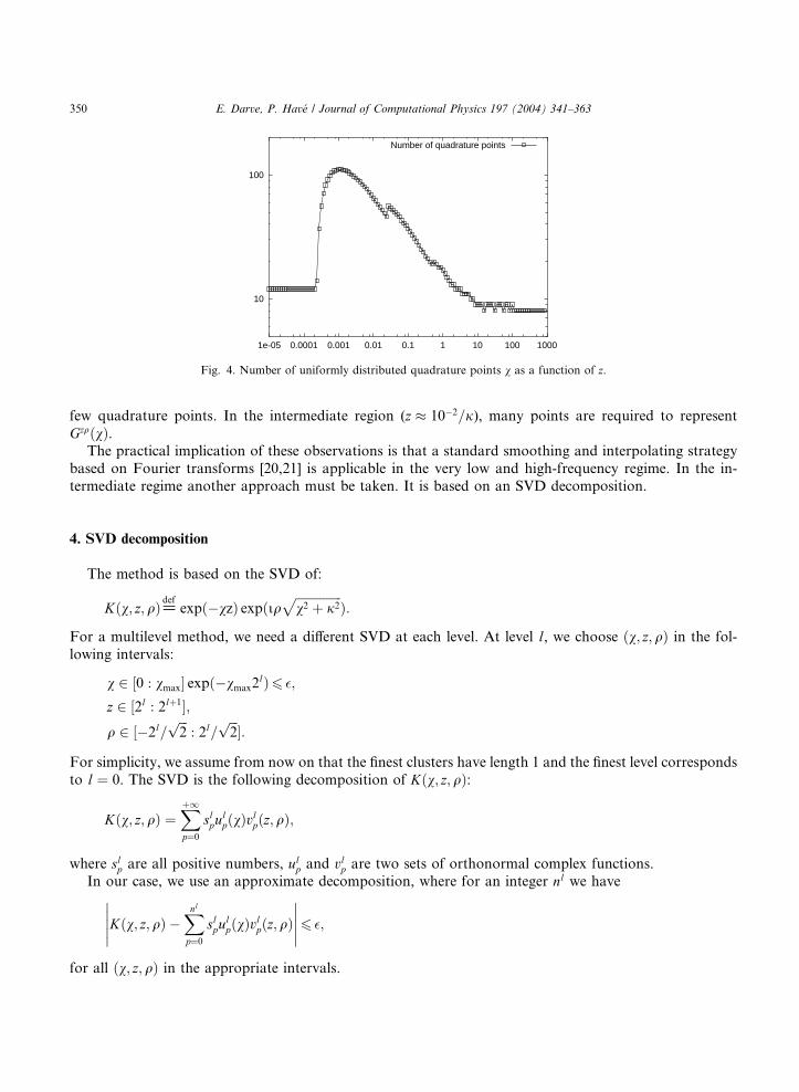
Fig. 4. Number of uniformly distributed quadrature points v as a function of z.


few quadrature points. In the intermediate region (z � 10�2=j), many points are required to represent

GzqðvÞ.The practical implication of these observations is that a standard smoothing and interpolating strategy

based on Fourier transforms [20,21] is applicable in the very low and high-frequency regime. In the in-

termediate regime another approach must be taken. It is based on an SVD decomposition.

4. SVD decomposition

The method is based on the SVD of:

Kðv; z; qÞ@def expð�vzÞ expðiqffiffiffiffiffiffiffiffiffiffiffiffiffiffiffiv2 þ j2

pÞ:

For a multilevel method, we need a different SVD at each level. At level l, we choose ðv; z; qÞ in the fol-

lowing intervals:

v 2 ½0 : vmax� expð�vmax2lÞ6 �;

z 2 ½2l : 2lþ1�;q 2 ½�2l=

ffiffiffi2

p: 2l=

ffiffiffi2

p�:

For simplicity, we assume from now on that the finest clusters have length 1 and the finest level corresponds

to l ¼ 0. The SVD is the following decomposition of Kðv; z; qÞ:

Kðv; z; qÞ ¼Xþ1

p¼0

slpulpðvÞvlpðz; qÞ;

where slp are all positive numbers, ulp and vlp are two sets of orthonormal complex functions.

In our case, we use an approximate decomposition, where for an integer nl we have

Kðv; z; qÞ��

Xnlp¼0

slpulpðvÞvlpðz; qÞ

��6 �;

for all ðv; z; qÞ in the appropriate intervals.


For more details on this decomposition and how to compute it numerically see [44].

Numerical tests show that a small number of coefficients is needed to efficiently approximate Kðv; z; qÞ.For example, for z ¼ 10�3, we computed the number of quadrature points p as function of the error �. Wecan observe (Fig. 5) that p is Oðlog �Þ.

In the low-frequency regime, the largest number of quadrature points given by SVD for � ¼ 10�6 is 10

(Fig. 6), which is much better than before (see Fig. 4 with a maximum above 100). Moreover, for very low-

frequency and high-frequency regimes, the quadrature is always smaller than with uniformly distributed

points.

To take advantage of the SVD decomposition, we compute the following variables, for each cluster Cla at

level l:

ka;lp ð/Þ ¼Z vmax

0

ðulpðvÞÞ� X

i

JiKðv; zi

� za;lk ; ðxi � xa;lk Þ cos/þ ðyi � ya;lk Þ sin/Þ

!dv:

The sum is over all sources located at ðxi; yi; ziÞ in cluster Cla, and of intensity Ji. We denote Ol

a the center of

Cla and rl the length of the side of the cluster. With these notations, the reference center ðxa;lk ; ya;lk ; za;lk Þ must

be located at the following point:

xa;lk ¼ xOla;

ya;lk ¼ yOla;

za;lk ¼ zOlaþ 3

2rl:

8><>:

Proposition 4. The choice of ðxa;lk ; ya;lk ; za;lk Þ is optimal in the sense that for a given error �, we have a minimal

number of terms in the SVD decomposition.

Proof. Let us introduce a parameter a and choose the reference center at:

0

2

4

6

8

10

12

14

1e-09 1e-08 1e-07 1e-06 1e-05 0.0001 0.001 0.01 0.1


Fig. 5. Number of quadrature points v as function of �, given by SVD.

0

2

4

6

8

10

1e-07 1e-06 1e-05 0.0001 0.001 0.01 0.1 1 10 100


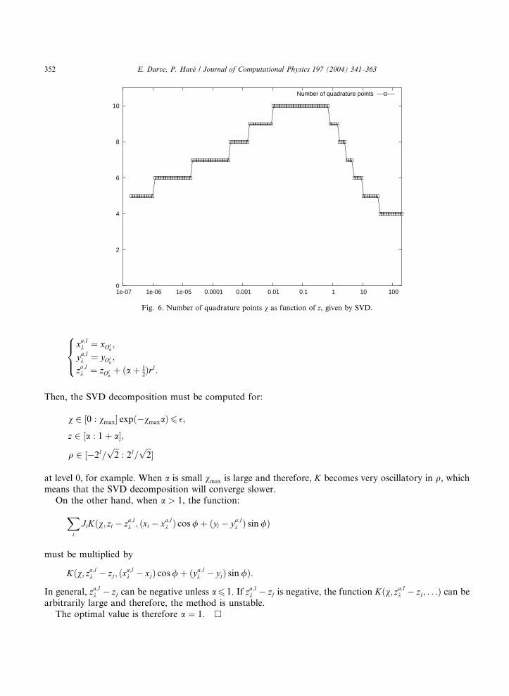
Fig. 6. Number of quadrature points v as function of z, given by SVD.


xa;lk ¼ xOla;

ya;lk ¼ yOla;

za;lk ¼ zOlaþ ðaþ 1

2Þrl:

8><>:

Then, the SVD decomposition must be computed for:

v 2 ½0 : vmax� expð�vmaxaÞ6 �;

z 2 ½a : 1þ a�;

q 2 ½�2l=ffiffiffi2

p: 2l=

ffiffiffi2

p�

at level 0, for example. When a is small vmax is large and therefore, K becomes very oscillatory in q, whichmeans that the SVD decomposition will converge slower.

On the other hand, when a > 1, the function:

Xi

JiKðv; zi � za;lk ; ðxi � xa;lk Þ cos/þ ðyi � ya;lk Þ sin/Þ

must be multiplied by

Kðv; za;lk � zj; ðxa;lk � xjÞ cos/þ ðya;lk � yjÞ sin/Þ:

In general, za;lk � zj can be negative unless a6 1. If za;lk � zj is negative, the function Kðv; za;lk � zj; . . .Þ can be

arbitrarily large and therefore, the method is unstable.

The optimal value is therefore a ¼ 1. �


We now introduce the following matrix:

Mlpqðz; x cos/þ y sin/Þ ¼

Zðulþ1

p ðvÞÞ�Kðv; z; x cos/þ y sin/ÞulqðvÞdv:

Proposition 5. Assume that cluster Clþ1b is the parent of cluster Cl

a. Then,

kb;lþ1p ð/Þ

�� Xnlq¼1

Mlpqðz; x cos/þ y sin/Þka;lq ð/Þ

��6 �;

where

x ¼ xa;lk � xb;lþ1k ;

y ¼ ya;lk � yb;lþ1k ;

z ¼ za;lk � zb;lþ1k :

8><>:

Proof. Use the SVD decomposition of K,

Kðv; z; qÞ �Xnlp¼0

slpulpðvÞvlpðz; qÞ;

and the fact that ulþ1p ðvÞ is an orthonormal basis. �

The scattering phase is done in the same manner, albeit with the transpose of Mpq. We introduce the

following coefficients:

la;lp ð/Þ ¼

Z vmax

0

ulpðvÞXi

JiKðv; zi

� za;ll ; ðxi � xa;ll Þ cos/þ ðyi � ya;ll Þ sin/Þ

!dv

for all sources i far away from cluster Cla, where now

xa;ll ¼ xOla;

ya;ll ¼ yOla;

za;ll ¼ zOla� 3

2rl:

8<:

The following proposition is true:

Proposition 6. Assume that cluster Clþ1b is the parent of cluster Cl

a. Then

la;lp ð/Þ

�� Xnlþ1

q¼1

Mlqpðz; x cos/þ y sin/Þlb;lþ1

q ð/Þ��6 �

slp; ð11Þ

where

x ¼ xb;lþ1l � xa;ll ;

y ¼ yb;lþ1l � ya;ll ;

z ¼ zb;lþ1l � za;ll :

8<:


Proof. Let us denote q0 ¼ ðxi � xb;lþ1l Þ cos/þ ðyi � yb;lþ1

l Þ sin/ for a given i and z0 ¼ zi � zb;lþ1l . Then

Xnlþ1

q¼1

Mlqp

Z vmax

0

ulþ1q ðvÞKðv; z0; q0Þdv ¼

ZdvulpðvÞKðv; z; x cos/þ y sin/Þ

Xnlþ1

q¼1

ðulþ1q ðvÞÞ�

Z vmax

0

ulþ1q ðvÞKðv; z0; q0Þdv:

The proof would be straightforward if

Kðv; z0; q0Þ �Xnlþ1

q¼1

ðulþ1q ðvÞÞ�

Z vmax

0

ulþ1q ðvÞKðv; z0; q0Þdv:

However, this is not true in general.

The following identity can be proved:

Mlpq ¼

slþ1p

slq

Zðvlqðz; qÞÞ

�vlþ1p ðzþ zab; qþ xab cos/þ yab sin/Þdzdq; ð12Þ

with xab ¼ xb;lþ1l � xa;ll , yab ¼ yb;lþ1

l � ya;ll and zab ¼ zb;lþ1l � za;ll .

With this identity

Xnlþ1

q¼1

Mlqp

Z vmax

0

ulþ1q ðvÞKðv; z0; q0Þdv � 1

slp

Z vmax

0

dvZ

dzdqðvlqðz; qÞÞ�Kðv; z; qÞ

Kðv; z0 þ zab; q0 þ xab cos/þ yab sin/Þ

¼Z vmax

0

dvulqðvÞKðv; zi � za;ll ; ðxi � xa;ll Þ cos/þ ðyi � ya;ll Þ sin/Þ

¼ la;lp ð/Þ:

The error is bounded by the difference

Kðv; z�� þ zab;qþ xab cos/þ yab sin/Þ �

Xnlþ1

q¼1

slþ1q ulþ1

q ðvÞvlþ1q ðzþ zab;qþ xab cos/þ yab sin/Þ

��6 �: �

The bound �=slp means that for large p the coefficients are calculated less accurately than for small p.However, this does not affect the accuracy of the final result for the matrix vector product, since the po-

tential at location rj is obtained using:Xp

slpvlpðz; qÞla;l

p ð/Þ:

The error on the matrix vector product is therefore smaller than �.After applying Eq. (11), we are using an approximation to la;l

p ð/Þ, ~la;lp ð/Þ, for which

la;lp ð/Þ

�� ~la;lp ð/Þ

��6 �

slp:

We prove that bound (11) remains valid when we use ~la;lp ð/Þ instead of la;l

p ð/Þ.


Proposition 7. Assume that

lb;lþ1q ð/Þ

�� ~lb;lþ1q ð/Þ

��6 �

slþ1q

;

for all q, then

la;lp ð/Þ

�� Xnlþ1

q¼1

Mlqpðz; x cos/þ y sin/Þ~lb;lþ1

q ð/Þ��6 �

slp:

This is essential to ensure the accuracy of the multilevel scheme.

Proof. Use Eq. (12).

Inner-to-Outer transform. Rokhlin and Yarvin [44] introduced a method of generalized Gaussian

quadratures to integrate Kðv; z; qÞ over v for a certain range of z and q. This quadrature can be used tocompute la;l

p ð/Þ from ka;lp ð/Þ. This is done in the following way.

We start by computingXp

ka;lp ð/ÞulpðvÞ:

This is an approximation of

Xp

ka;lp ð/ÞulpðvÞ��

Xi

JiKðv; zi � za;lk ; ðxi � xa;lk Þ cos/þ ðyi � ya;lk Þ sin/Þ��6 �:

We multiply by

Kðv; za;lk � zb;ll ; ðxa;lk � xb;ll Þ cos/þ ðya;lk � yb;ll Þ sin/Þ@def T lbaðv;/Þ: �

We now prove that

Proposition 8. The generalized Gaussian quadrature can be used to compute the integral over v of:

la;lq ð/Þ ¼

ZulqðvÞ

Xb

T lbaðv;/Þ

Xp

ka;lp ð/ÞulpðvÞ !( )

dv;

with accuracy �=slq.

Proof. Assume we are at level 0 and the size of the cluster is 1. Consider the following approximation basedon an SVD:

Kðv; z; qÞ��

Xmp¼1

spupðvÞvpðz; qÞ��6 �;

for any v 2 ½0 : vmax�, vmax ¼ log 1=�, z 2 ½1 : 4� and q 2 ½�4ffiffiffi2

p: 4

ffiffiffi2

p�.

Using this approximation, we construct a generalized Gaussian quadrature with m=2 points vk and

weights xk. Consider two clusters C0a and C0

b such that C0b is in the interaction list of C0

a , and two points

ðxi; yi; ziÞ 2 C0a and ðx; y; zÞ 2 C0

b . Then,


ZKðv; zi

�� z; ðxi � xÞ cos/þ ðyi � yÞ sin/Þdv

�Xm=2k¼1

xkKðvk; zi � z; ðxi � xÞ cos/þ ðyi � yÞ sin/Þ��6 �:

We have

Kðv; zi � z; ðxi � xÞ cos/þ ðyi � yÞ sin/Þ ¼ Kðv; zb;0k � z; ðxb;0k � xÞ cos/þ ðyb;0k � yÞ sin/Þ

T 0baðv;/Þ Kðv; zi � za;0k ; ðxi � xa;0k Þ cos/

þ ðyi � ya;0k Þ sin/Þ:

By applying the SVD to Kðv; zb;0k � z; ðxb;0k � xÞ cos/þ ðyb;0k � yÞ sin/Þ and using the fact that v0pðz; qÞ is anorthonormal basis, we have proved that ðvk;xkÞ can integrateZ

s0qu0qðvÞT 0

baðv;/ÞKðv; zi � za;0k ; ðxi � xa;0k Þ cos/þ ðyi � ya;0k Þ sin/Þdv;

with accuracy �. Therefore, the error on lb;0q ð/Þ is of the order of �=s0q. The same proof is applicable to any

level l. �

5. Numerical tests

In will section, we will illustrate the stability for a wide frequency range of the method by some examples

of our code. All results are obtained by an EFIE formulation without preconditioning.

For these tests, we have used l0 ¼ 1:25751 10�6, �0 ¼ 8:84806 10�12 giving c ¼ 299792548:2 m=s; theobjects are perfectly conductive.

The targeted error is 10�4 for the Kernel approximation, and the iterative solver (GMRES) stops when

the residual becomes below than 10�4.

5.1. Low-frequency regime: sphere k=15

This example (Fig. 7) shows a radar cross-section (RCS) on the unit sphere of 3000 edges (dof) with a

wavelength k ¼ 30. The exact solution is done by Mie Series.

This example has failed using the standard plane wave expansion (see Eq. (2)), even for three levels, the

lowest number of levels for the FMM. This was due to numerical instabilities in the transfer functions

Tp;rðrÞ (Eq. (3)).The propagative term has been discretized with 4 7 points (variable r) at level 3 and seven points for v

for the evanescent term.

5.2. Intermediate-frequency regime: sphere 2k

This example (Fig. 8) shows a RCS on the unit sphere of 3000 edges with a wave length k ¼ 1. The exact

solution is done by Mie Series.

The standard plane wave expansion has failed on this example when we are using more than five levels.

The propagative term has been discretized with 16 31 points (variable r) at level 3, 10 19 at level 4,

and with five and six points for v for the evanescent term.

-50

-40

-30

-20

-10

0

10

20

0 0.5 1 1.5 2 2.5 3

RC

S (

dB)

Observation Angle

RCS

Numerical RCSexact RCS [sphere R=1]

Fig. 8. RCS of unit sphere of size 2k.

-60

-50

-40

-30

-20

-10

0 0.5 1 1.5 2 2.5 3

RC

S (

dB)

Observation Angle

RCS

Numerical RCSexact RCS [sphere R=1]

Fig. 7. RCS of the unit sphere of size k=15.


5.3. High-frequency regime: sphere 5:5k

This example (Fig. 9) shows an RCS on unit sphere of 18,000 edges with a wave length k ¼ 0:36. Theexact solution is done by Mie Series.

-20

-15

-10

-5

0

5

10

15

20

25

30

0 0.5 1 1.5 2 2.5 3 3.5

RC

S (

dB)

Observation Angle

RCS

Numerical RCSExact RCS [sphere R=1]

Fig. 9. RCS of unit sphere of size 5:5k.


The propagative term has been discretized with 26 71 points at level 3, 20 39 points at level 4 and

four points for v for the evanescent term.

5.4. Comparison of the stable plane wave FMM and the low-frequency MLFMA

The stable plane wave FMM (SPW-FMM) and low-frequency MLFMA (LF-MLFMA) can both be

used to solve low-frequency electromagnetic scattering. In this section, we compare their memory re-quirement and computational expense in a range of frequency from j ¼ 10�4 to j ¼ 10.

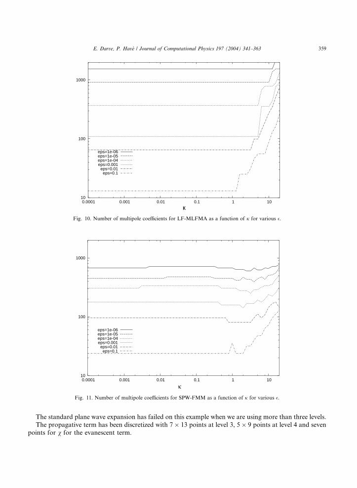
Figs. 10 and 11 show the memory requirement, which is estimated using the size of the discretization

for a single cluster of radius 1, i.e., the number of multipole coefficients. LF-MLFMA values are esti-

mations based on the worst convergence case in Eq. (1). This worst case is given by the transfer vector

r ¼ ð2; 0; 0Þ and a local transfer vector r0 ¼ ð1; 1; 1Þ. Those memory requirements appear to be very

similar.

Regarding the computational cost, Figs. 12 and 13 show the benefit of our new expansion for the Inner-

to-Outer step (the most expensive step in both methods). This cost is given as the number of floating pointoperations for one Inner-to-Outer step. LF-MLFMA values are 2ðnFMAÞ2 flops, where nFMA is the dis-

cretization size. This corresponds to the cost of a matrix–vector product of size nFMA. SPW-FMM values

are 4nSPW flops, where nSPW is the discretization size. This corresponds to the cost of a complex term-by-

term product. SPW-FMM Inner-to-Outer cost is an order of magnitude below than LF-MLFMA for all

frequencies.

5.5. Car k=2

This example (Fig. 14) shows the electric intensity on the surface of a car of 18,000 edges with a wave

length k ¼ 30.

10

100

1000

0.0001 0.001 0.01 0.1 1 10

eps=1e-06eps=1e-05eps=1e-04eps=0.001

eps=0.01eps=0.1

κFig. 10. Number of multipole coefficients for LF-MLFMA as a function of j for various �.

10

100

1000

0.0001 0.001 0.01 0.1 1 10


eps=0.01eps=0.1

k

Fig. 11. Number of multipole coefficients for SPW-FMM as a function of j for various �.


The standard plane wave expansion has failed on this example when we are using more than three levels.

The propagative term has been discretized with 7 13 points at level 3, 5 9 points at level 4 and seven

points for v for the evanescent term.

100

1000

10000

100000

1e+06

1e+07

0.0001 0.001 0.01 0.1 1 10

eps=1e-06eps=1e-05eps=1e-04eps=0.001eps=0.01eps=0.1

k

Fig. 12. Computational cost of the Inner-to-Outer step for LF-MLFMA as a function of j for various �.

100

1000

10000

100000

1e+06

1e+07

0.0001 0.001 0.01 0.1 1 10


eps=0.01eps=0.1

k

Fig. 13. Computational cost of the Inner-to-Outer step for SPW-FMM as a function of j for various �.


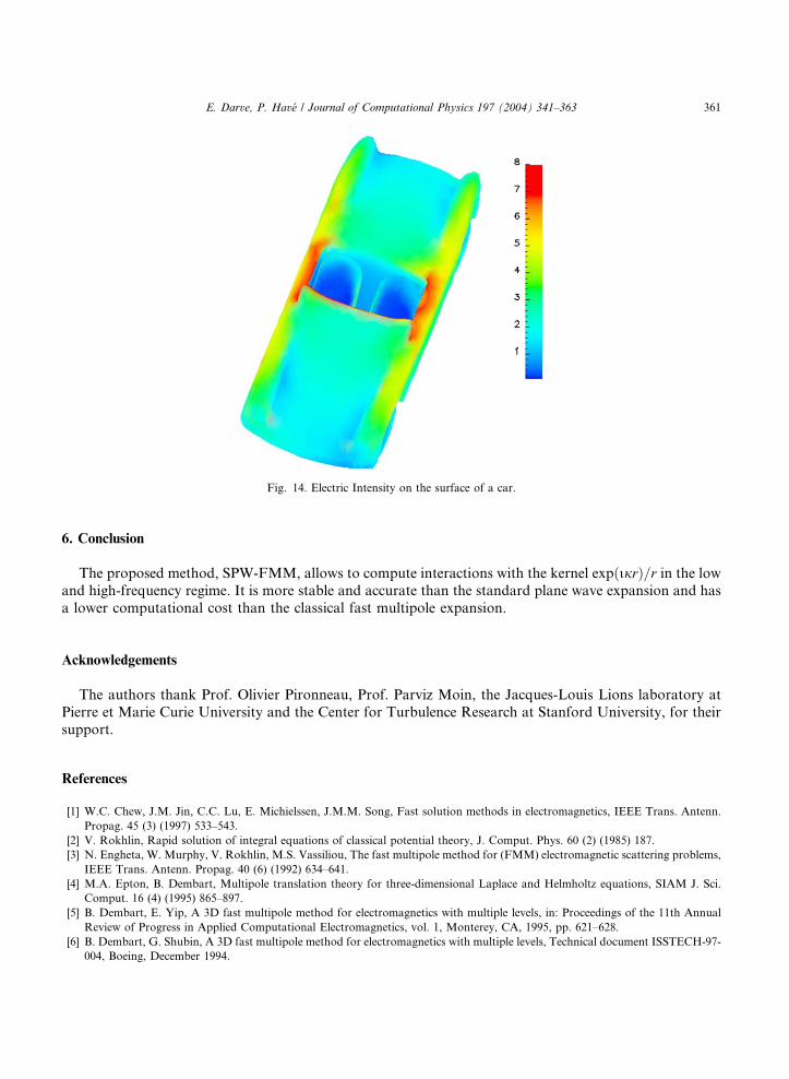
Fig. 14. Electric Intensity on the surface of a car.


6. Conclusion

The proposed method, SPW-FMM, allows to compute interactions with the kernel expðijrÞ=r in the low

and high-frequency regime. It is more stable and accurate than the standard plane wave expansion and has

a lower computational cost than the classical fast multipole expansion.

Acknowledgements

The authors thank Prof. Olivier Pironneau, Prof. Parviz Moin, the Jacques-Louis Lions laboratory at

Pierre et Marie Curie University and the Center for Turbulence Research at Stanford University, for their

support.

References

[1] W.C. Chew, J.M. Jin, C.C. Lu, E. Michielssen, J.M.M. Song, Fast solution methods in electromagnetics, IEEE Trans. Antenn.

Propag. 45 (3) (1997) 533–543.

[2] V. Rokhlin, Rapid solution of integral equations of classical potential theory, J. Comput. Phys. 60 (2) (1985) 187.

[3] N. Engheta, W. Murphy, V. Rokhlin, M.S. Vassiliou, The fast multipole method for (FMM) electromagnetic scattering problems,

IEEE Trans. Antenn. Propag. 40 (6) (1992) 634–641.

[4] M.A. Epton, B. Dembart, Multipole translation theory for three-dimensional Laplace and Helmholtz equations, SIAM J. Sci.

Comput. 16 (4) (1995) 865–897.

[5] B. Dembart, E. Yip, A 3D fast multipole method for electromagnetics with multiple levels, in: Proceedings of the 11th Annual

Review of Progress in Applied Computational Electromagnetics, vol. 1, Monterey, CA, 1995, pp. 621–628.

[6] B. Dembart, G. Shubin, A 3D fast multipole method for electromagnetics with multiple levels, Technical document ISSTECH-97-

004, Boeing, December 1994.


[7] B. Dembart, E. Yip, A 3-D moment method code based on fast multipole, in: URSI Radio Science Meeting Dig., Seattle, WA,

1994, p. 23.

[8] W. Elliott, J. Board, Fast Fourier-transform accelerated fast multipole algorithm, SIAM J. Sci. Comput. 17 (2) (1996) 398–415.

[9] L.Greengard,V.Rokhlin,Anewversionof the fastmultipolemethod for theLaplace equation in threedimensions,ActaNumer. 229.

[10] C. White, M. Headgordon, Rotating around the quartic angular-momentum barrier in fast multipole method calculations, J.

Chem. Phys. 105 (12) (1996) 5061–5067.

[11] J.-S. Zhao, W.C. Chew, Applying matrix rotation to the three-dimensional low-frequency multilevel fast multipole algorithm,

Microw. Opt. Technol. Lett. 26 (2) (2000) 105–110.

[12] L. Greengard, J. Huang, V. Rokhlin, S. Wandzura, Accelerating fast multipole methods for low frequency scattering, IEEE

Comput. Sci. Engrg. Mag.

[13] J.-S. Zhao, W.C. Chew, Three-dimensional multilevel fast multipole algorithm from static to electrodynamic, Microw. Opt.

Technol. Lett. 26 (1) (2000) 43–48.

[14] J.-S. Zhao, W.C. Chew, MLFMA for solving integral equations of 2-D electromagnetic problems from static to electrodynamic,

Microw. Opt. Technol. Lett. 20 (5) (1999) 306–311.

[15] J.-S. Zhao, W.C. Chew, Applying LF-MLFMA to solve complex PEC structures, Microw. Opt. Technol. Lett. 28 (3) (2001) 155–

160.

[16] V. Rokhlin, Rapid solution of integral equations of scattering theory in two dimensions, J. Comput. Phys. 86 (2) (1990) 414–439.

[17] V. Rokhlin, Diagonal forms of translation operators for the Helmholtz equation in three dimensions, Research Report YALEU/

DCS/RR-894, Department of Computer Science, Yale University, March 1992.

[18] C.C. Lu, W.C. Chew, A multilevel algorithm for solving boundary-value scattering, Microw. Opt. Technol. Lett. 7 (10) (1994)

466–470.

[19] J. Song, C.-C. Lu, W.C. Chew, Multilevel fast multipole algorithm for electromagnetic scattering by large complex objects, IEEE

Trans. Antenn. Propag. 45 (10) (1997) 1488–1493.

[20] E. Darve, The fast multipole method (i): error analysis and asymptotic complexity, SIAM Numer. Anal. 38 (1) (2000) 98–128.

[21] E. Darve, The fast multipole method: numerical implementation, J. Comput. Phys. 160 (1) (2000) 195–240.

[22] W.C. Chew, Fast algorithms for wave scattering developed at the University of Illinois�s electromagnetics laboratory, IEEE

Antenn. Propag. Mag. 35 (4) (1993) 22–32.

[23] W.C. Chew, J. Jin, C.-C. Lu, E. Michielssen, J. Song, Fast solution methods in electromagnetics, IEEE Trans. Antenn. Propag. 45

(3) (1997) 533–543.

[24] J. Song, W.C. Chew, Multilevel fast-multipole algorithm for solving combined field integral equations of electromagnetic

scattering, Microw. Opt. Technol. Lett. 10 (1) (1995) 14–19.

[25] W.C. Chew, C.-C. Lu, Y.M. Wang, Review of efficient computation of three-dimensional scattering of vector electromagnetic

waves, J. Opt. Soc. Am. A 11 (1994) 1528–1537.

[26] C.C. Lu, W.C. Chew, Fast far-field approximation for calculating the RCS of large objects, Microw. Opt. Technol. Lett. 8 (5).

[27] J. Song, C.-C. Lu, W.C. Chew, S. Lee, Fast Illinois solver code (FISC) solves problems of unprecedented size at the center for

computational electromagnetics, University of Illinois Technical Report CCEM-23-97, University of Illinois, Urbana Champaign,

IL, 1997.

[28] J. Song, C. Lu, W.C. Chew, S. Lee, Fast Illinois solver code (FISC), IEEE Antenn. Propag. Mag. 40 (3) (1998) 27–33.

[29] C. Lu, W.C. Chew, A multilevel algorithm for solving a boundary integral equation of wave scattering, Microw. Opt. Technol.

Lett. 7 (10) (1994) 466–470.

[30] R.L. Wagner, W.C. Chew, A ray-propagation fast multipole algorithm, Microw. Opt. Technol. Lett. 7 (10) (1994) 435–438.

[31] J. Song, W.C. Chew, Error analysis for the truncation of multipole expansion of vector Green�s functions, IEEEMicrow. Wireless

Comp. Lett. 11 (7) (2001) 311–313.

[32] S. Koc, J. Song, W.C. Chew, Error analysis for the numerical evaluation of the diagonal forms of the scalar spherical addition

theorem, SIAM J. Numer. Anal. 36 (3) (1999) 906–921.

[33] D. Solvason, H. Petersen, Error estimates for the fast multipole method, J. Statist. Phys. 86 (1–2) (1997) 391–420.

[34] S. Amini, A. Profit, Analysis of the truncation errors in the fast multipole method for scattering problems, J. Comput. Appl.

Math. 115 (1–2) (2000) 23–33.

[35] B. Dembart, E. Yip, The accuracy of fast multipole methods for Maxwell�s equations, IEEE Comput. Sci. Engrg. 5 (3) (1998) 48–

56.

[36] S. Bindiganavale, J. Volakis, Guidelines for using the fast multipole method to calculate the RCS of large objects, Microw. Opt.

Technol. Lett. 11 (4) (1996) 190–194.

[37] S. Ohnuki, W.C. Chew, A study of the error controllability of MLFMA, Antennas and Propagation Society, IEEE. Int. Symp. 3

(2001) 774–777.

[38] B. Hu, W.C. Chew, Fast inhomogeneous plane wave algorithm for multi-layered medium problems, in: IEEE Antennas and

Propagation Society International Symposium, Transmitting Waves of Progress to the Next Millennium, Salt Lake City, UT,

2000, pp. 606–609.


[39] B. Hu, W.C. Chew, E. Michielssen, J. Zhao, Fast inhomogeneous plane wave algorithm (FIPWA) for the fast analysis of two-

dimensional scattering problems, University of Illinois, Urbana.

[40] B. Hu, C. Chew, W.E. Michielssen, J. Zhao, Fast inhomogeneous plane wave algorithm for the fast analysis of two-dimensional

scattering problems, Radio Sci. 34 (4) (1999) 759–772.

[41] B. Hu, W.C. Chew, Fast inhomogeneous plane wave algorithm for electromagnetic solutions in layered medium structures: two-

dimensional case, Radio Sci. 35 (1) (2000) 31–43.

[42] B. Hu, C. Chew, W.S. Velamparambil, Fast inhomogeneous plane analysis of electromagnetic wave algorithm for the scattering,

Radio Sci. 36 (6) (2001) 1327–1340.

[43] B. Hu, W.C. Chew, Fast inhomogeneous plane wave algorithm for scattering from objects above the multilayered medium, IEEE

Trans. Geosci. Remote Sensing 39 (5) (2001) 1028–1038.

[44] N. Yarvin, V. Rokhlin, Generalized Gaussian quadratures and singular value decompositions of integral operators, Technical

Report 1109, Department of Computer Science Research Report, Yale University, 1996.

Eï¬ƒcient fast multipole method for low-frequency scattering

Documents

Transcript of Eï¬ƒcient fast multipole method for low-frequency scattering