An Efficient Discontinuous Galerkin Method

for Advective Transport in Porous Media ?

Jostein R. Natvig a,∗ Knut–Andreas Lie a,b Birgitte Eikemo c

Inga Berre c

aSINTEF ICT, Department of Applied Mathematics, P.O. Box 124 Blindern,NO–0314 Oslo, Norway

bCentre of Mathematics for Applications, University of Oslo, P.O. Box 1053Blindern, NO–0316 Oslo, Norway

cUniversity of Bergen, Deptartment of Mathematics, Johs. Brunsgt. 12, NO-5008Bergen, Norway

Abstract

We consider a discontinuous Galerkin scheme for computing transport in hetero-geneous media. An efficient solution of the resulting linear system of equations ispossible by taking advantage of a priori knowledge of the direction of flow. Byarranging the elements in a suitable sequence, one does not need to assemble thefull system and may compute the solution in an element-by-element fashion. Wedemonstrate this procedure on boundary-value problems for tracer transport andtime-of-flight.

Key words: transport in porous media, time-of-flight, discontinuous Galerkindiscretization, linear solvers, directed asyclic graphs

? The research was funded in part by the Research Council of Norway under grantsno. 139144/431 and 158908/I30.∗ Corresponding author.

Email addresses: Jostein.R.Natvig@sintef.no (Jostein R. Natvig),Knut-Andreas.Lie@sintef.no (Knut–Andreas Lie), birgitte@mi.uib.no(Birgitte Eikemo), ingab@mi.uib.no (Inga Berre).

Preprint submitted to Advances in Water Resources 16 May 2007

1 Introduction

In this paper, we consider efficient and accurate methods for a class of linearequations on the form

v · ∇u = H(u,x), for x ∈ Ω,

u = h(x), for x ∈ ∂Ω−,(1)

where v is a given (divergence-free) vector field and ∂Ω− denotes the inflowboundary of Ω. Our motivation for studying this equation comes from trans-port in porous media, where equations on this form are used as simple trans-port models or arise as the result of a semi-discretisation of a more complextransport equation. Accurate solution of (1) is of great importance in areassuch as oil recovery and groundwater hydrology because (1) reveals the trans-port properties of v. Solving (1) is rather easy for smooth v, but becomesmuch harder when the vector field has large spatial variations and exhibitsfine-scale details that are important for the global flow pattern.

In the following, we focus on convective transport in a porous medium com-pletely filled with fluids of a single phase. To this end, we assume that thefluid velocity v is a time-independent function that is given as the result ofa finite-volume or a (mixed) finite-element computation. In reservoir simula-tion, for instance, it is common to use a low-order method to compute theflux defined on a grid rather than the flow velocity v, meaning that v will begiven in terms of flux values that typically are constant on each element facein the grid.

To discretise (1), we will use a discontinuous Galerkin (dG) method for theoperator v · ∇ in combination with an upwind approximation of the flux.The discontinuous Galerkin method was introduced by Reed and Hill [17]for the problem of neutron transport. LeSaint and Raviart [14] analysed themethod in this context and proved a rate of convergence of O(∆xn) for smoothsolutions on Cartesian grids. A number of researchers have made significantcontributions since then. Among others, Lin and Zhou [13] proved convergenceof the method for nonsmooth solutions. Moreover, Cockburn and Shu [2,3]analysed and extended the original discontinuous Galerkin method to systemsof hyperbolic conservation laws and convection-dominated problems.

It is interesting to note that (1) can be interpreted as a stationary advectionequation with a source term, and it is therefore close to the original applica-tion of Reed and Hill. However, the problem we address in this paper is theresolution of advective transport when v varies many orders of magnitude,whereas Reed and Hill consider a smooth velocity field.

The dG discretisation of (1) will lead to a large system of (non)linear equa-

2

tions. However, due to the directional derivative v · ∇, the exact solution ineach grid cell K only depends on the set of points on the upstream side ofa bundle of streamlines passing through K and is independent of the solu-tion elsewhere in the domain. Using an upwind flux in our dG discretisationpreserves this one-sided domain of dependence, and it is therefore possible tocompute the solution in one element at a time, from inflow to outflow bound-aries, if we can find a sequence of elements so that element i appears afterelement j in the sequence if i depend on j. Using arguments from graph theory,we will show that such a sequence can be found in linear time by traversingthe grid and visiting each grid cell once. This optimal sequence of elementscan then be exploited to develop a very efficient (non)linear solver based ona reordering of the unknowns giving a upper block-triangular system. Thisway, the computational effort needed to solve (1) is reduced from solving alarge sparse (non)linear system involving all degrees-of-freedom in the domain,to solving a sequence of smaller problems involving one or a few (non)linearequations. In the linear case, this gives a direct solver that is not only sim-ple to implement, but also fast and inexpensive in terms of storage. In thenonlinear case, one has to apply an iterative solver for each subproblem. Theresulting solver will generally have better convergence than a correspondingsolver for the full system, since the iterations can be controlled independentlyin each subproblem. We note that these ideas are not new. The reduction of amatrix to block-triangular form by use of depth-first traversal of elements wasdescribed in Duff et al. [7]. Similarly, Dennis et al. [6] explore the use of block-triangular structures to construct effective Newton-type nonlinear solvers. Asfar as we know, however, these ideas have not been used to compute transportin porous media.

In this paper we will mainly focus on the case where H(u) is a linear functionof u. Extensions of the methodology to more general nonlinear equations ofthe form v·∇F (u) = H(u,x) (arising e.g., from an implicit semi-discretizationof multiphase-multicomponent transport models) are discussed in a separatepaper [15]. In Section 2, we derive a few basic transport models on the form(1). Our motivating examples will be two linear boundary-value problems,one for the stationary distribution of tracers and one for the so-called time-of-flight. Isocontours of time-of-flight represent the time-lines in a reservoirand the corresponding differential equation exhibits all the difficulties seen inmore complex transport models due to nonsmooth spatial variations in theforcing velocity field. The time-of-flight equation will therefore be our keyexample used to develop the methodology. Solutions of the stationary tracerequation have a much simpler structure and are only used herein as a meansto delineate reservoirs with multiple wells into (nearly) independent flow re-gions. In Section 3, we introduce the discontinuous Galerkin method brieflyand present the variational formulation and discretisation of (1). Then, inSection 4 we show how to solve the corresponding linear system efficientlyusing a reordering strategy. In Section 5, we show how to compute the distri-

3

bution of tracers from multiple wells in a single-phase reservoir. In Section 6,we present some numerical examples for computation of time-of-flight from(5) and compare the accuracy of our dG methods to highly resolved solutionsobtained by pointwise integration of streamlines. Finally, Section 7 containssome concluding remarks.

2 Basic Transport Models

The flow of fluids through porous and heterogeneous media can be modelledas a set of balance laws for the conservation of mass for each fluid component.For a mixture of m fluid components separated into ` phases, we have

∑i=1

(∂t(φcαiρisi) +∇ · (cαiviρi)

)=

∑i=1

cαiqi, α = 1, . . . ,m, (2)

where φ is the porosity of the medium; ρi, si, vi, and qi are the density,saturation (volume fraction), phase velocity, and volumetric source term ofthe i’th phase; and cαi is the mass fraction of component α in phase i. In thismodel gravity and capillary effects have been neglected.

If all fluids are of the same phase (i.e., ` = 1) and the flow is incompressible,we can write down the equation for the bulk motion of the fluid componentsin terms of the common fluid pressure p and the volumetric velocity field v:

∇ · v = q/ρ, v = −K

µ∇p. (3)

Here K is the permeability of the medium and µ is the viscosity. The linearrelation between average fluid velocity and pressure gradients is called Darcy’slaw. For simplicity, we scale (3) such that µ = 1 and assume that q consistsof a set of point-sources modelling injection/production wells.

The indvidual distribution of the various components are now given in termsof linear transport equations, ∂t(φcα)+∇·(cαv) = cαq/ρ. In other words, eachfluid component is transported according to the volumetric velocity field v. Asour first example of such a transport model, we consider the stationary distri-bution of a set of passive tracers (α = 1, . . . ,m) and assume incompressibleflow. Equation (2) then simplifies to

v · ∇cα = 0.

We remark that gravity can be included these simple transport equationsby replacing Darcy’s law in (3) by v = −K(∇p − ρg)/µ. In Section 5 wewill use the stationary tracer tranport equation as a means for computing

4

connectivity between sites for injecting and producing fluids, thereby derivingreservoir compartmentalisation.

For flows with more than one phase, one can derive a pressure equation of theform (3), where K/µ is replaced by Kλ(s) and λ(s) is a nonlinear functionaccounting for the reduced mobility due to the presence of more than onefluid phase. As for single-phase flow, the motion of fluids is, in the absenceof gravity, aligned with the velocity field v; thus, all instantaneous transportoccurs along integral curves Ψ of v.

Integral curves, or streamlines, Ψ are everywhere tangent to the velocity fieldv. If we introduce the bistream functions ξ, η, given such that v = ∇ξ×∇η, theintegral curves of v map to straight lines (ξ =const, η =const) in the so-calledstreamline coordinates (τ, ξ, η). Here τ takes the role of the spatial coordinatealong streamlines and is called the time-of-flight coordinate. Moreover, wehave the operator identity

v · ∇ = φ∂τ . (4)

The appearance of φ in this relation is convenient since φ rescales streamlinecoordinate according to the pore volume the streamline passes through. For ahomogeneous medium, however, τ equals the standard curve length along Ψafter an aproriate scaling (corresponding to setting φ = 1).

The simplest possible model of the form (1) for convective transport inducedby v, is the following boundary-value problem for time-of-flight τ in Ω,

v · ∇τ = φ, τ |x∈∂Ω− = 0. (5)

The equation follows trivially by applying the operator identity (4) to thestreamline coordinate τ . The time-of-flight τ(x) measures the time it takes apassive particle released at the closest point on the inflow boundary to travel toa given point x. Isocontours of τ(x) are the time-lines in the porous mediumand as such give vital information about the flow pattern, in particular forsingle-phase flow. The time-of-flight is also a cornerstone in modern streamlinemethods, see [5,11]. In a streamline setting, τ(x) is usually given by the integral

τ(x) =∫Ψ

φ ds

|v|, (6)

evaluated along the streamline Ψ connecting x to the inflow boundary ∂Ω−.

Another interesting sub-case of (1) arises if we apply an implicit temporaldiscretisation to the transport equations (2), giving equations of the form

un − un−1

∆t+∇ · (vun) = q. (7)

5

By using the product rule on the term ∇· (vun) and a discontinuous Galerkinmethod for spatial discretisation of v · ∇un, we will get essentially the samelinear systems for each time step as for (5), but with a different right-handside.

3 Discontinuous Galerkin Discretisation

The discretisation in a discontinuous Galerkin method starts with a variationalformulation as in a standard Galerkin method, but allows for discontinuitiesover the element edges. To get the variational formulation of (1), we partitionthe domain into a collection of non-overlapping elements K. Let V be thespace of arbitrarily smooth test functions. By multiplying (1) with a functionv ∈ V and integrating by parts over each element K, we get

−∫

K(uv) · ∇v dx +

∫∂K

(uv) · n v ds =∫

KH(u,x)v dx ∀ v ∈ V,

where n is the outer normal on the element boundary ∂K. We seek solutionsin a finite-dimensional subspace Vh ⊂ V , so we replace the exact solution andthe test function by uh ∈ Vh and vh ∈ Vh, respectively. For Vh, we choose thespace of piecewise smooth functions that may be discontinuous over elementboundaries. Since uh may be discontinuous over inter-element boundaries, wemust replace the flux term (uv ·n) by a consistent and conservative numericalflux function f(a, b,v · n). This leads to the following discrete variationalformulation: let

aK(uh, vh) = −∫

K(uhv) · ∇vh dx +

∫∂K

f(uh, uexth ,v · n) vh ds,

bK(uh, vh) =∫

KH(uh,x) vh dx,

and find uh such that

aK(uh, vh) = bK(uh, vh) ∀ K, ∀ vh ∈ Vh. (8)

Here f is the upwind flux given by

f(p, pext,v · n) = p max(v · n, 0) + pext min(v · n, 0), (9)

for inner and outer approximations p and pext at the element boundaries. Theupwind flux preserves the directional dependency in the solution, which iscrucial in our solution procedure.

To fix ideas, we assume, for simplicity of presentation, that Ω ⊂ R2 andassume that the elements K are rectangles in a regular Cartesian grid. LetQn = spanxpyq : 0 ≤ p, q ≤ n be the space of polynomials of degree at most

6

n in x and at most n in y, and let V(n)h = v : v|K ∈ Qn. A convenient basis

for this space is the tensor product of Legendre polynomials Lk = `r(x)`s(y)for r, s = 0, . . . , n. The approximate solution on an element Ki can then bewritten as

uh(x, y) =n2∑

k=0

tik Lk

(2(x− xi)

∆xi,2(y − yi)

∆yi

), (10)

where (xi, yi) is the centre of element Ki. Thus, V(0)h is the space of elementwise

constant functions and yields a formally first-order accurate scheme, V(1)h is

the space of elementwise bilinear approximations and yields a formally second-order accurate scheme, etc. In the following, we use dG(n) to denote thediscontinuous Galerkin approximation of polynomial order n. In other words,the error of a dG(n)-method will decay with order n+1 for smooth solutions.On nonsmooth solutions, slower convergence is to be expected. Finally, thedegrees of freedom per element in a dG(n)-method is m = (n+1)d in d spatialdimensions.

4 Fast Solution by Reordering the Unknowns

In the following we will motivate and present the optimal reordering thatallows us to solve (8) elementwise. To this end, we will use the time-of-flightequation (5), for which (8) simplifies to a linear system

aK(uh, vh) = bK(vh) ∀ K, ∀ vh ∈ Vh. (11)

Although (8) and (11) have different structure on a given element K, the twoglobal systems will have a similar block structure. All ideas presented for thelinear case (11) will therefore immediately carry over to the nonlinear case(8).

By substituting the approximate solution (10) and the tensor-product Leg-endre polynomials in the variational formulation (11), we get a set of linearequations for the degrees-of-freedom in each element. Let T denote the vectorof unknown coefficients tik in all of Ω, and let TK be the vector of unknownsfor element K. In element K, we have

AKT = BK , AKT = −RK TK + FKT

where (AK) ij = ahK(Li, Lj) and (BK)i = bh

K(Li), and ahK and bh

K are numericalapproximations to the integrals in (11) using Gaussian quadrature. For con-venience, we have split the coefficient matrix into the element stiffness matrixR and the coupling to other elements through the numerical flux integral F .

7

The coefficient matrix has a block-banded structure, where the size of eachblock is given by the number of unknowns in each element.

The properties of F are in general determined by the choice of numerical flux.The upwind flux (9) can be written as

FKT = F+KTK + F−

KTU(K), (12)

where F+ denotes flux out of element K, F− denotes flux into element K,and we write U(K) for the set of neighbouring elements on the upwind sideof K, i.e., U(K) = E ∈ Ω : ∂E ∩ ∂K− 6= ∅. Thus, the system reads

−RK TK + F+K TK = BK − F−

K TU(K). (13)

The split F = (F+ + F−) is easy to motivate and understand if one assumesthat v ·n does not change sign on element interfaces, which we will do hence-forth. If v is computed using a standard low-order discretisation method for(3) like the two-point flux-approximation method (i.e., the five-point methodin 2D) or the lowest-order Raviart–Thomas mixed finite-element method, v ·nwill typically be constant on each element face. In this case, U(K) consists ofall elements E such that (v · n)|∂E∩∂K < 0, where n is the outward-pointingnormal to K.

The key to an efficient solution procedure is to take advantage of the fact that(1) has this one-sided domain of dependence; in other words, both the exactand the numerical solution in any element is determined by the solution on theupstream side(s). Thus, we can construct the solution in a given element oncethe solution is known in the element’s immediate upstream neighbours. Bycareful inspection, we may therefore construct the solution locally, starting atsources or inflow boundaries and proceeding downstream. A similar approachwas used in [17] in the context of neutron transport. To our knowledge, theidea has never been applied to transport in porous media before.

From a computational point of view, it is more convenient to look at this asa reordering of unknowns. Observe that we can solve (13) element by elementif we can determine a sequence of elements such that i appears before j in thesequence if there is a flux from element Ki to element Kj. By processing theelements in such a sequence, the right-hand side of (13) is a known quantityin each step. Since the directions of the fluxes are determined solely by v (andnot by T), this sequence can be computed as part of a preprocessing stepbefore solving the system (13).

The idea of solving boundary-value problems for advective transport sequen-tially by a reordering of unknowns was also used in [1], but with a differentspatial discretisation. In that paper, we used an algorithm to compute a suit-able sequence based on physical arguments. The solution was constructed by

8

11 15 16

51 4

32 7 8

6

1413129

10 10 14 16

61 5

42 8 12

9

1513113

7

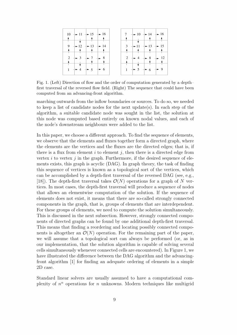
Fig. 1. (Left) Direction of flow and the order of computation generated by a depth–first traversal of the reversed flow field. (Right) The sequence that could have beencomputed from an advancing-front algorithm.

marching outwards from the inflow boundaries or sources. To do so, we neededto keep a list of candidate nodes for the next update(s). In each step of thealgorithm, a suitable candidate node was sought in the list, the solution atthis node was computed based entirely on known nodal values, and each ofthe node’s downstream neighbours were added to the list.

In this paper, we choose a different approach. To find the sequence of elements,we observe that the elements and fluxes together form a directed graph, wherethe elements are the vertices and the fluxes are the directed edges; that is, ifthere is a flux from element i to element j, then there is a directed edge fromvertex i to vertex j in the graph. Furthermore, if the desired sequence of ele-ments exists, this graph is acyclic (DAG). In graph theory, the task of findingthis sequence of vertices is known as a topological sort of the vertices, whichcan be accomplished by a depth-first traversal of the reversed DAG (see, e.g.,[18]). The depth-first traversal takes O(N) operations for a graph of N ver-tices. In most cases, the depth-first traversal will produce a sequence of nodesthat allows an elementwise computation of the solution. If the sequence ofelements does not exist, it means that there are so-called strongly connectedcomponents in the graph, that is, groups of elements that are interdependent.For these groups of elements, we need to compute the solution simultaneously.This is discussed in the next subsection. However, strongly connected compo-nents of directed graphs can be found by one additional depth-first traversal.This means that finding a reordering and locating possibly connected compo-nents is altogether an O(N) operation. For the remaining part of the paper,we will assume that a topological sort can always be performed (or, as inour implementation, that the solution algorithm is capable of solving severalcells simultaneously whenever connected cells are encountered). In Figure 1, wehave illustrated the difference between the DAG algorithm and the advancing-front algorithm [1] for finding an adequate ordering of elements in a simple2D case.

Standard linear solvers are usually assumed to have a computational com-plexity of nα operations for n unknowns. Modern techniques like multigrid

9

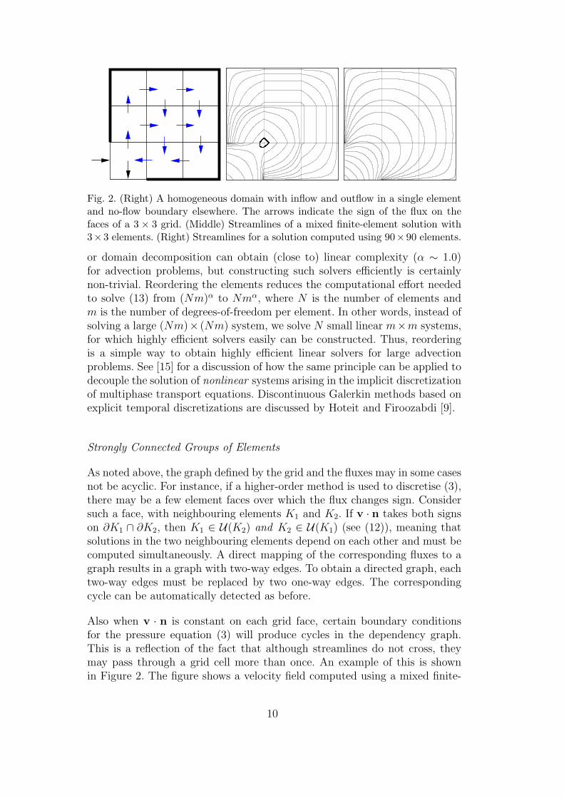
Fig. 2. (Right) A homogeneous domain with inflow and outflow in a single elementand no-flow boundary elsewhere. The arrows indicate the sign of the flux on thefaces of a 3 × 3 grid. (Middle) Streamlines of a mixed finite-element solution with3×3 elements. (Right) Streamlines for a solution computed using 90×90 elements.

or domain decomposition can obtain (close to) linear complexity (α ∼ 1.0)for advection problems, but constructing such solvers efficiently is certainlynon-trivial. Reordering the elements reduces the computational effort neededto solve (13) from (Nm)α to Nmα, where N is the number of elements andm is the number of degrees-of-freedom per element. In other words, instead ofsolving a large (Nm)× (Nm) system, we solve N small linear m×m systems,for which highly efficient solvers easily can be constructed. Thus, reorderingis a simple way to obtain highly efficient linear solvers for large advectionproblems. See [15] for a discussion of how the same principle can be applied todecouple the solution of nonlinear systems arising in the implicit discretizationof multiphase transport equations. Discontinuous Galerkin methods based onexplicit temporal discretizations are discussed by Hoteit and Firoozabdi [9].

Strongly Connected Groups of Elements

As noted above, the graph defined by the grid and the fluxes may in some casesnot be acyclic. For instance, if a higher-order method is used to discretise (3),there may be a few element faces over which the flux changes sign. Considersuch a face, with neighbouring elements K1 and K2. If v · n takes both signson ∂K1 ∩ ∂K2, then K1 ∈ U(K2) and K2 ∈ U(K1) (see (12)), meaning thatsolutions in the two neighbouring elements depend on each other and must becomputed simultaneously. A direct mapping of the corresponding fluxes to agraph results in a graph with two-way edges. To obtain a directed graph, eachtwo-way edges must be replaced by two one-way edges. The correspondingcycle can be automatically detected as before.

Also when v · n is constant on each grid face, certain boundary conditionsfor the pressure equation (3) will produce cycles in the dependency graph.This is a reflection of the fact that although streamlines do not cross, theymay pass through a grid cell more than once. An example of this is shownin Figure 2. The figure shows a velocity field computed using a mixed finite-

10

9 9 13

109

1 2 3 4

75

9

12

11

86

Fig. 3. The figure shows a suitable sequence of computations when a group ofconnected elements is encountered.

element method with lowest order Raviart–Thomas on a coarse and on afine grid. The velocity field is the solution of (3) with the imposed boundaryconditions shown. When the global inflow and outflow boundaries are edgesof the same element, every streamline starts and ends in this element. Thus,the dependency graph of the elements will not be acyclic. In fact, for this caseall the degrees-of-freedom in the domain must be computed simultaneously.Note also that a more accurate solution of (3) projected onto the 3 × 3 gridproduces the same dependency graph.

The situation in Figure 2 is a worst-case scenario. A more likely distributionof fluxes is depicted in Figure 3, where a small subset of elements are stronglyconnected. In this situation, our reordering strategy still works and gives onelarger linear system associated with the 2× 2 block of interconnected cells inaddition to the usual twelve linear systems associated with single cells.

Moreover, blocks of interconnected cells do not appear if one uses a two-pointflux-approximation finite-volume scheme for the pressure equation (3), as hasbeen the standard in the oil industry. A simple argument of decreasing pressurealong streamlines rules out the possibility of a streamline re-entering a cell.

5 Approximation of Tracer Distribution

Determining the spatial region swept by a fluid source or an inflow boundary,or vice versa, the spatial region from which fluid is drained by a sink or anoutflow boundary, is of practical importance both in groundwater managementand petroleum engineering. In reservoir engineering, computing streamlines iswell suited for predicting where fluid from different wells will eventually endup. For incompressible flow, any streamline in the domain connects two wells,an injector and a producer. Thus, by assigning a unique label to each well,streamlines will give information about well connectivity and areas affectedby each injector or producer. The way one could obtain the same informationin a finite-volume method is by computing the transport of tracers from each

11

injector. When the tracer transport becomes stationary, one would obtaininformation about well connectivity and affected areas.

Our ideas lend themselves naturally to compute the transport of tracer effec-tively. The stationary distribution of tracers is given by an equation of theform

v · ∇c = 0, c|x∈∂Ω− given. (14)

Since c is constant along streamlines, the solution to this equation can be deter-mined in each point by tracing a streamline backward to the inflow boundary.

To determine the reservoir volume connected to a particular injector, we wouldsolve (14) by setting the concentration of tracer component i to 1 in well i and0 in the m− 1 other wells and compute the tracer distribution in the non-wellblocks. For an upwind discontinuous Galerkin discretisation of equation (14),the linear equations for element K are

(−RK + F+K + F−

K )Ci = 0, i = 1, . . . ,m, (15)

where Ci is the vector of unknowns for tracer i. As before, we may split thevector of unknowns Ci in the unknowns Ci, K for element K and the unknownsCi, U(K) in the neighbouring upwind elements. Then, (15) may be written as

−RKCi,K + F+KCi,K = −F−

KCi, U(K), i = 1, . . . ,m.

By solving this equation for C in one element at a time, we compute thedistribution of tracers in the domain. Note that the tracer components areindependent so only one matrix factorisation is needed for the solution of anm-tracer problem. The same idea can easily be extended to compressible flows,for which (14) is replaced by v · ∇c = −c∇ · v.

From the tracer distribution, we can approximate the swept areas of eachinjection well. The simplest approach is to draw the 0.5 contour (isosurface)of each tracer concentration. To obtain the drained areas for each productionwell, we simply reverse the velocity field. To get the well connectivity, we cancombine the two calculations to uniquely determine the part of the domainaffected by a given injector-producer pair.

At this point it might be tempting to ask why one could not replace (14) bya simple graph colouring algorithm to assign a colour to all nodes influencedby a particular injector (or more generally, a particular part of the inflowboundary). Such an approach is indeed possible, but would in general lead tomulti-labelled nodes. Due to the fluxes, our directed graph is a weighted graph.By solving the tracer equation (15), we are effectively computing a weightedcolouring of the graph.

12

Swept Areas/Volumes

We will now present three test cases, in which we use the above idea to de-lineate reservoirs in 2D and 3D, respectively. To this end, we compute thestationary distribution of one tracer launched from each injector. In the fig-ures, we show the swept areas/volumes, which are distinguished by differentshading. In 2D, the boundaries of the regions are marked by black and corre-spond to the 0.5 contour of each tracer concentration.

We first show how this idea works in two space dimensions. To asses the per-formance of the method, we will use geological data from Model 2 of the 10thSPE Comparative Solution Project [4]. The model contains 60 × 220 × 85cells and consists of two formations: a shallow-marine Tarbert formation inthe top 35 layers, where the permeability is relatively smooth, and a fluivialUpper-Ness permeability in the bottom 50 layers. Both formations are char-acterised by large permeability variations, 8–12 orders of magnitude, but arequalitatively different; see Figure 9 for plots of the corresponding permeabil-ities. We compute the swept areas of eight injectors placed on the boundaryof two rectangular reservoirs corresponding to Layers 1 and 76 Three produc-tion wells are placed inside the domain so that the wells form three five-spotpatterns. The production wells are sources with rate -2.0, the injection wellsin the corners have rate +0.5, and the other injection wells have rate +1.0. Inthe figures, the production wells are marked by white and injection wells byblack circles.

Figure 4 shows the swept areas for Layers 1 and 76, respectively, computedusing the dG(0) and dG(1) methods. To illustrate the flow directions, a fewstreamlines are plotted in the domain. In the figures, these are drawn in white.The streamlines close to the boundaries between the swept areas make itpossible to evaluate the quality of the approximations for different orders ofthe dG discretisation.

The permeability in Layer 1 is relatively smooth, and the differences betweenthe dG(0) and dG(1) discretisations are minor. The permeability in Layer 76,has a strongly heterogeneous structure with intertwined high-permeable chan-nels on a low-permeable background. Using the dG(0) method, we can observesome streamlines crossing the boundaries between the swept areas, whereasthe dG(1) method seems to have captured the areas correctly. Increasing theorder in the dG discretization further did not produce any observable differ-ences in the swept areas.

The same idea can also be applied to three-dimensional problems. Figure 5shows swept volumes computed for the fifteen upper layers of the SPE 10 testcase. The injection wells are located in the upper-left and upper-right cornersof the back plane and in the lower-left and lower-right corner in the front plane.

13

Layer 1

Layer 76

Fig. 4. The plots show the tracer distribution for two layers of the SPE 10 test case.The solution is computed using the dG(0) (upper) and dG(1) (lower).

The production well is placed in the centre of the domain. To distinguish theswept regions for each tracer, we have applied different shadings.

Table 1 reports runtimes for a similar partitioning of the full SPE 10 modelwith 1 122 000 cells. The runtimes have been split into time used to reorder andtime used for solving the local dense m×m systems with LAPACK. For com-pleteness we have also included corresponding timings for dG with tri-linearand tri-quadratic basis functions (P-basis). By using the first-order dG(0) dis-cretization, the whole 1.1 million reservoir model is delineated in only a fewseconds, which means that the method has a big potential for use in interac-tive user-exploration of large geomodels. If more accuracy is required for theswept volumes, the corresponding runtime will of course increase significantly.However, by using the P-basis, a second-order approximation is computed in

14

Fig. 5. Tracer distribution for a subsample from the smooth Tarbert formation in theSPE 10 test case. The velocity is computed using a two-point flux approximation.

Table 1CPU time in seconds used to reorder and to solve the tracer boundary-value problemfor the SPE 10 five-spot reservoir using dG(n) with m degrees of freedoms per cell.Runtimes are measured on a single core on an AMD Athlon X2 4400+ processor.

n basis m reorder solve total

0 — 1 1.24 1.87 3.11

1 P-basis 4 1.21 8.65 9.86

1 Q-basis 8 1.20 25.22 26.41

2 P-basis 10 1.21 85.28 86.48

2 Q-basis 27 1.20 582.34 583.53

less than ten seconds and a third-order approximation in less than 1.5 min-utes. (Notice also that for dG(2), the total number of unknowns is more than30 millions).

6 Approximation of Time-of-Flight

In this section we will discuss the approximation of the time-of-flight equation(5) through a series of test cases with increasing difficulty. Although the equa-tion has a simple form, the solutions are useful in many applications of trans-port in porous media. In ground-water flow, for instance, the time-of-flight canbe used to identify the areas affected by a contamination. Moreover, as theexamples in this section will clearly demonstrate, time-of-flight holds much of

15

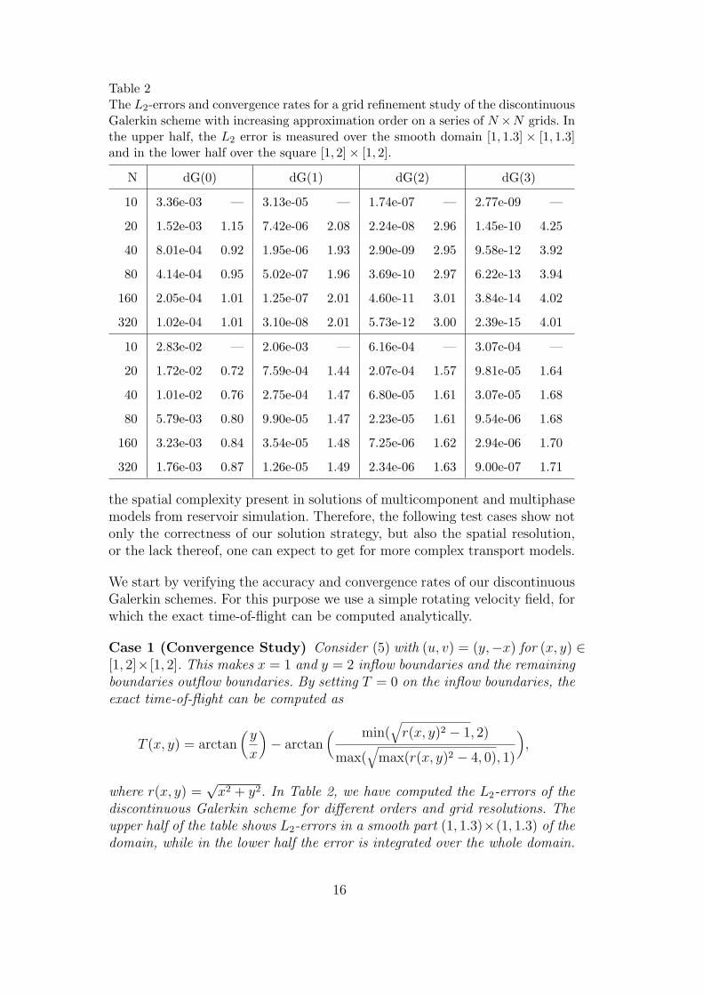
Table 2The L2-errors and convergence rates for a grid refinement study of the discontinuousGalerkin scheme with increasing approximation order on a series of N ×N grids. Inthe upper half, the L2 error is measured over the smooth domain [1, 1.3] × [1, 1.3]and in the lower half over the square [1, 2]× [1, 2].

N dG(0) dG(1) dG(2) dG(3)

10 3.36e-03 — 3.13e-05 — 1.74e-07 — 2.77e-09 —

20 1.52e-03 1.15 7.42e-06 2.08 2.24e-08 2.96 1.45e-10 4.25

40 8.01e-04 0.92 1.95e-06 1.93 2.90e-09 2.95 9.58e-12 3.92

80 4.14e-04 0.95 5.02e-07 1.96 3.69e-10 2.97 6.22e-13 3.94

160 2.05e-04 1.01 1.25e-07 2.01 4.60e-11 3.01 3.84e-14 4.02

320 1.02e-04 1.01 3.10e-08 2.01 5.73e-12 3.00 2.39e-15 4.01

10 2.83e-02 — 2.06e-03 — 6.16e-04 — 3.07e-04 —

20 1.72e-02 0.72 7.59e-04 1.44 2.07e-04 1.57 9.81e-05 1.64

40 1.01e-02 0.76 2.75e-04 1.47 6.80e-05 1.61 3.07e-05 1.68

80 5.79e-03 0.80 9.90e-05 1.47 2.23e-05 1.61 9.54e-06 1.68

160 3.23e-03 0.84 3.54e-05 1.48 7.25e-06 1.62 2.94e-06 1.70

320 1.76e-03 0.87 1.26e-05 1.49 2.34e-06 1.63 9.00e-07 1.71

the spatial complexity present in solutions of multicomponent and multiphasemodels from reservoir simulation. Therefore, the following test cases show notonly the correctness of our solution strategy, but also the spatial resolution,or the lack thereof, one can expect to get for more complex transport models.

We start by verifying the accuracy and convergence rates of our discontinuousGalerkin schemes. For this purpose we use a simple rotating velocity field, forwhich the exact time-of-flight can be computed analytically.

Case 1 (Convergence Study) Consider (5) with (u, v) = (y,−x) for (x, y) ∈[1, 2]× [1, 2]. This makes x = 1 and y = 2 inflow boundaries and the remainingboundaries outflow boundaries. By setting T = 0 on the inflow boundaries, theexact time-of-flight can be computed as

T (x, y) = arctan(

y

x

)− arctan

( min(√

r(x, y)2 − 1, 2)

max(√

max(r(x, y)2 − 4, 0), 1)

),

where r(x, y) =√

x2 + y2. In Table 2, we have computed the L2-errors of thediscontinuous Galerkin scheme for different orders and grid resolutions. Theupper half of the table shows L2-errors in a smooth part (1, 1.3)×(1, 1.3) of thedomain, while in the lower half the error is integrated over the whole domain.

16

The dG methods yield the expected order of accuracy in smooth regions, butdue to the kink in the solution along the circular arc r =

√5, we get reduced

convergence rates for the whole domain.

For applications in porous media the velocity field v is typically obtained bysolving a pressure equation of the form (3). In the remaining examples ofthis section we will compare grid-based solutions obtained by discontinuousGalerkin methods of varying order to highly resolved streamline solutions ob-tained by back-tracing streamlines from a set of 10× 10 uniformly distributedpoints within each element. Unless stated otherwise, the same subresolutionis used in all the following plots to evaluate the piecewise polynomial dG-solutions within each element.

In all examples, we assume that v is known and given in a such way that theflux v · n is constant over each element face in a Cartesian grid. We can thenuse a streamline tracing method due to Pollock [16] to compute highly resolvedreference solutions. Pollock’s method uses an exact formula for the streamlinethrough each element based upon a piecewise linear approximation of v ineach direction. The method is widely used in the petroleum industry to tracestreamlines, even though it may become highly inaccurate for non-Cartesiangrids, see [10].

The first example is a standard test case in oil reservoir simulation, called aquarter-five spot:

Case 2 (Heterogeneous Quarter Five-Spot) Consider a reservoir con-sisting of the unit square with no-flow boundaries and with a source placedin the lower-left corner and a sink in the upper-right corner. The syntheticpermeability field is lognormal and isotropic and spans six orders of magni-tude from the smallest to the largest value and the porosity is assumed to beconstant equal unity. The corresponding (single-phase) velocity field is com-puted using a mixed finite-element method with first-order Raviart–Thomasbasis on 129× 129 elements.

Figure 6 compares solutions computed by the dG(n) scheme for n = 0, 1, 2with the solution obtained by the node-based fast-sweeping scheme of [1] (forwhich no subsampling was used in the plotting). In addition, we have includeda reference solution obtained by tracing streamlines with Pollock’s method[16] from 10 × 10 uniformly distributed points inside each element. Pollock’smethod reproduces the exact time-of-flight since the velocity field computed bythe lowest-order Raviart–Thomas approximation is consistent with the velocityapproximation used in the tracing algorithm. The fast-sweeping method givesa resolution that is slightly better than dG(0) and slightly worse than dG(1).The differences are easily explained if we momentarily interpret dG(0) as afirst-order finite-difference scheme. Whereas dG(0) uses a first-order upwind

17

dG(0) fast-sweeping

dG(1) dG(2)

streamline reference

Fig. 6. Time-of-flights for Case 2 computed using dG(n) for n = 0, 1, 2, thefast-sweeping method, and direct streamline integration. The contours in the plotsare T = 0.07, . . . , 0.49 PVI in steps of 0.07.

18

discretisation in each coordinate direction corresponding to a five-point stencil,the fast-sweeping method uses a first-order upwind discretisation along localstreamlines, which corresponds to a nine-point stencil and should therefore bemore accurate. In the plots, it also appears to be smoother than dG(0), but thisis a plotting artifact due to the linear interpolation inherent in the contouringalgorithm. (For dG(0) we effectively use a piecewise constant interpolation dueto the 10× 10 subsampling).

Finally, we notice that the third-order method agrees remarkably well with thehighly-resolved streamline reference solution.

In our second reservoir example we consider a three-dimensional case withsimilar heterogeneity as in Case 2.

Case 3 We consider a reservoir model consisting of 64 × 64 × 16 grid cellswith unit porosity and a smoothed, lognormally distributed permeability fieldwith values spanning five orders of magnitude, see Figure 7. An injector islocated in the lower-left corner of the front face, a producer is located in theupper-right corner of the back face, and no-flow conditions are specified at theboundaries.

Figure 7 shows time-of-flights computed by dG(n) for n = 0, 1, 2. As in Case 2,dG(0) resolves the main features of the heterogeneous flow field, but underes-timates the penetration of sharp fluid fingers. By increasing the polynomialorder in the dG-basis functions, we allow for sub-cell variation in the time-of-flight and thereby improve the resolution of the viscous fingering, which in asense is a sub-grid phenomenon.

In the absence of gravity effects, (hyperbolic) models for multiphase and mul-ticomponent transport will typically have only positive characteristics. Thismeans that time-of-flight carries important information about the temporaldevelopment of complex spatial structures in the solution and τ(x) can thus beused to infer much about flow patterns for convection-dominated transport. Inother words, by solving for τ(x) one can therefore learn much about the fluidmotion without having to compute all time steps of a full fluid simulation.

From a computational point-of-view, computing the time-of-flight is in a cer-tain sense more difficult than computing one time-step of a transport problemlike e.g., (7). For transport problems, data are given in the whole spatial do-main, and the domain of dependence for a single point (or grid cell) is thereforelimited by ∆t times the maximum wave speed associated by the correspond-ing continuous equation, and the variation in phase saturations or componentconcentrations are typically limited to the interval [0, 1]. Time-of-flight, on theother hand, has a global domain of dependence in the sense that τ(x) dependson all points along the streamline from x and back to the inflow boundary;see (6). Moreover, the time-of-flight values may easily span several orders of

19

Permeability dG(0)

dG(1) dG(2)

Fig. 7. Lognormal permeability field for Case 3 and corresponding time-of-flightscomputed using dG(n) for n = 0, 1, 2. The contours shown in the slice plots are atT = 0.1, . . . , 0.6 PVI in steps of 0.1.

magnitude.

In the two examples above, the reservoir heterogeneity was mild due to unitporosity and relatively smooth spatial variation in v. As a result, τ(x) hadrelatively smooth variation even though it contained the characteristic viscousfingers, and we were able to obtain good resolution by choosing a uniformsufficiently high order for the dG basis functions.

For highly heterogeneous reservoirs with large variations in the porosity orstrong shears in the velocity field, τ will generally have low regularity andexhibit very large variations. For instance, in regions where high-speed flowmeets low-speed flow from nearly impermeable regions such as channel wallsor obstacles, the time-of-flight may oscillate with orders of magnitude overa few elements. Use of higher-order polynomial approximations can thereforeeasily result in oscillations and unphysical time-of-flight values, as will bedemonstrated in Case 4. Moreover, if these variations are not captured by thelocal approximation, the error along the outflow edges will be propagated tothe neighbour elements.

20

Slope Limiting

Spurious oscillations is a common problem in many discontinuous Galerkinmethods and is usually circumvented by applying a (slope) limiter that re-duces the local variation of each basis function by modifying the coefficientsof polynomial terms of order two and higher. Limiters are usually derived froma maximum principle or from a principle that limits the local variation.

For the time-of-flight equation (5), the only principle available to us is thefact that τ(x) is strictly increasing along streamlines, which follows triviallyfrom (6). We therefore propose to check that the time-of-flight is higher onthe outflow edges than on the inflow edges of each element; that is,

min τ |∂K+ > (1− ε) max τ |∂K− , 0 ≤ ε 1.

If this is not the case, we recompute the solution in this element by making auniform subdivision into a set of first-order elements such that the number ofnew elements corresponds to the degrees-of-freedom in the original element.That is, for dG(1) we split the element in two in each spatial direction, fordG(2) we split in three, etc. By reducing the order to one, we expect to reducepossible oscillations, and by subdividing, we try to compensate for the reducedaccuracy associated with first-order elements.

To clearly demonstrate the problems caused by shear in the velocity field andthe effect of our order-reduction/subdivision strategy, we consider an artificialtransport problem with four large impermeable geometrical obstacles.

Case 4 We consider a quarter five-spot in a square domain with an injector inthe lower-left corner and a producer in the upper right. The permeability fieldconsists of a homogeneous background into which we have inserted four nearlyimpermeable obstacles—two triangles, a circle, and a rectangle—each having apermeability 10−6 relative to the background. The corresponding velocity field iscomputed using a mixed finite-element method with the lowest-order Raviart–Thomas basis.

As observed in [1], transport past obstacles and through channels is very chal-lenging since the time-of-flight field will have extreme gradients downstreamfrom the obstacles. In Figure 8 we compare two approximate solutions com-puted using dG(0) and dG(2) with the exact streamline solution. As above,the first-order scheme fails to capture the leading viscous fingers, in par-ticular those creeping around the impermeable circle. Similarly, the dG(2)solution contains strong oscillatory pollution that arise along impermeableboundaries and propagate in the downstream direction. By applying the order-reduction/subdivision strategy devised above with ε = 0.005, almost all theoscillations are removed and the exact solution is reproduced quite accurately.By only using order reduction and no subdivision, the corresponding dG(2)-

21

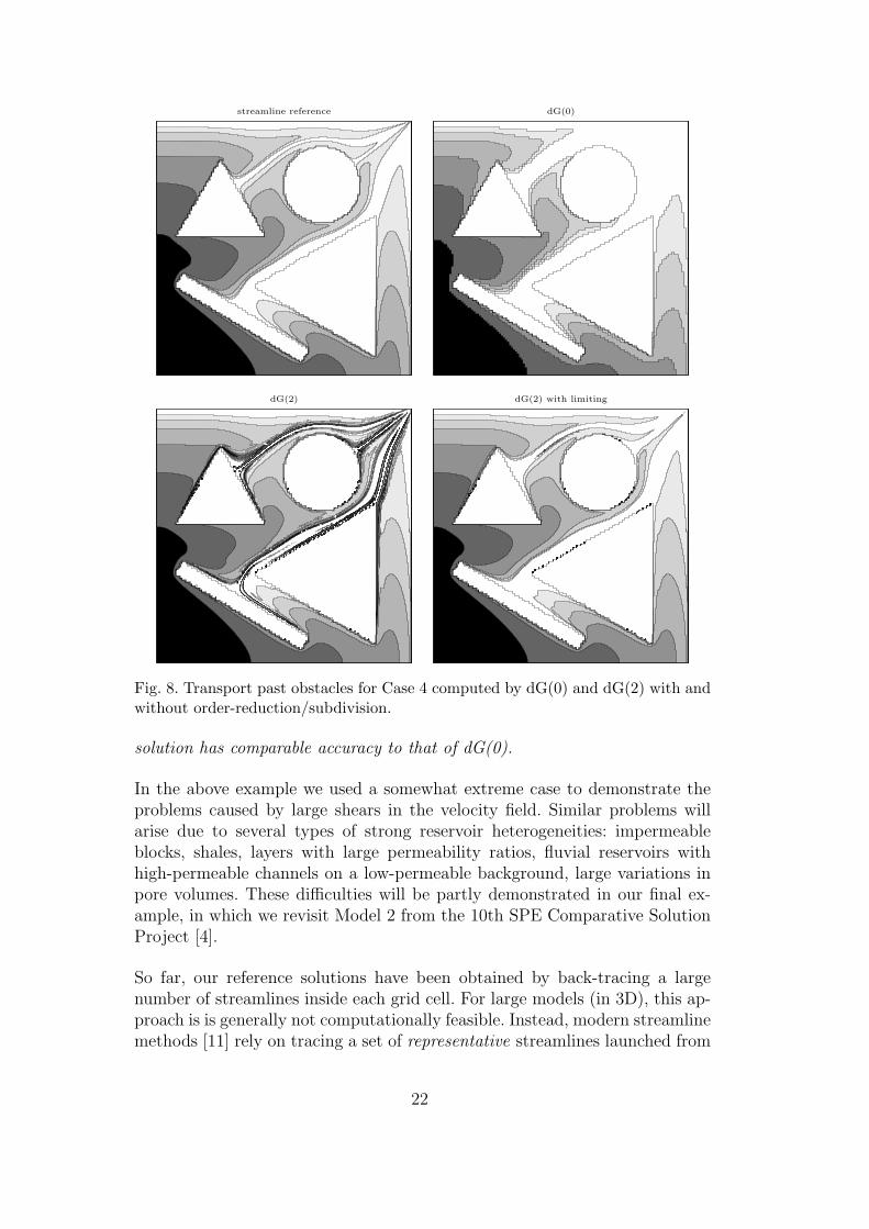
streamline reference dG(0)

dG(2) dG(2) with limiting

Fig. 8. Transport past obstacles for Case 4 computed by dG(0) and dG(2) with andwithout order-reduction/subdivision.

solution has comparable accuracy to that of dG(0).

In the above example we used a somewhat extreme case to demonstrate theproblems caused by large shears in the velocity field. Similar problems willarise due to several types of strong reservoir heterogeneities: impermeableblocks, shales, layers with large permeability ratios, fluvial reservoirs withhigh-permeable channels on a low-permeable background, large variations inpore volumes. These difficulties will be partly demonstrated in our final ex-ample, in which we revisit Model 2 from the 10th SPE Comparative SolutionProject [4].

So far, our reference solutions have been obtained by back-tracing a largenumber of streamlines inside each grid cell. For large models (in 3D), this ap-proach is is generally not computationally feasible. Instead, modern streamlinemethods [11] rely on tracing a set of representative streamlines launched from

22

Fig. 9. Permeability field and time-of-flight for Layers 1 (left) and 76 (right) of theSPE 10 test case computed with dG(n) for n = 0, 1, 2 (order increasing downwards),streamline solution with 1500 streamlines, and a streamline reference solution (bot-tom). The contours shown in the plots are at T = 0.1, . . . , 0.6 PVI in steps of 0.1for Layer 1 and T = 0.05, 0.1, 0.15 PVI for Layer 76.

injectors and/or producers; see e.g., [12]. Cell-values for time-of-flight can thenbe computed by averaging all streamlines passing through or in the neighbour-hood of each cell. This approach reduces the spatial accuracy unless one usesa sophisticated scheme for obtaining sufficient streamline coverage.

Case 5 In this example we consider two 2D quarter five-spot cases with per-meability and porosity data taken from Layers 1 and 76, respectively, of Model2 in the SPE 10 test case. Figure 9 shows the permeability and the corre-sponding time-of-flights computed by dG(n) for n = 0, 1, 2. For comparison wealso show solutions obtained by tracing 1500 streamlines initiated uniformlyfrom the well block. For the Tarbert formation in Layer 1, the variation inpermeability and porosity is relatively smooth. As in Case 2, dG(1) and dG(2)reproduce the qualitative behaviour of the solution, whereas dG(0) underesti-mates the viscous fingering. The accuracy of the standard streamline methodis somewhere between that of dG(1) and dG(2).

23

Fig. 10. Time-of-flight in the two grid cells (200, 36) and (200, 37) of Layer 76 inthe 10th SPE test case sampled in 2000×2000 evenly distributed points inside eachcell.

The fluvial Upper Ness formation in Layer 76 contains sharp contrasts inpermeability (and porosity) between the low-permeable background and a set ofintertwined high-permeable channels. For the higher-order dG methods we havetherefore applied our order-reduction/subdivision strategy. Figure 9 shows thatalthough dG(1) and dG(2) have quantitative errors, they are able to capturemost of the qualitative behaviour of the time-of-flight, which should be of mostinterest to a reservoir engineer. Moreover, the higher-order dG solutions areat least as accurate as the solution obtained by the standard streamline method.

To illustrate the difficulty of accurately resolving the time-of-flight in Layer 76,Figure 10 shows the exact solution sampled in 2000×2000 evenly spaced pointsinside two grid cells. Since time-of-flight is an integrated quantity, it is gen-erally not sufficient to capture the complex spatial behaviour inside each gridcell in an averaged sense. The variations in time-of-flight over a grid cell maybe quite large relative to an average value or a few representative point values.Any method based on either a low-order polynomial (as in dG(1) and dG(2)),or a few representative streamlines, is therefore bound to give quantitative er-rors, as observed in Figure 9.

7 Final Remarks

The purpose of this paper has been to explore the efficiency and accuracy of adiscontinuous Galerkin scheme applied to a class of boundary-value problemsfor advective transport. A unique feature of our methodology is the use of anoptimal ordering of the unknowns that allows us to compute the solutions inan element-by-element fashion.

We have demonstrated how one can use the framework to compute accurateapproximations to the stationary tracer distribution in a reservoir. This can

24

be used to compute so-called swept and drained areas/volumes and well con-nectivities. These quantities are usually computed using streamline methodsand have proved to be useful tools in, e.g., ranking and history matching. Dueto the efficient sequential solution procedure presented in this paper, this is aone-sweep computation that can be performed with high order accuracy andmodest demands on storage and computing power. Moreover, as our numericaltest cases illustrate, low-order approximations do, in general, provide sufficientaccuracy.

We have also demonstrated that the discontinuous Galerkin schemes in manycases can compute the time-of-flight with an accuracy comparable to stream-line approaches and superior to our earlier grid-based attempts [1]. For stronglyheterogeneous cases, direct integration of streamlines gives a spatial resolutionthat is hard to match with other methods based on grid points or cell vol-umes. One should therefore not expect grid-based methods to perform as wellas back-traced streamlines for all possible velocity fields, as was demonstratedin [1]. Indeed, we observe reduced accuracy for tranport past (and through)barriers and through channels as in Cases 4 and 5. For simple 2D cases onecan always argue that better results can be obtained by grid refinement orby tracing more streamlines, but this is less feasible, e.g., for the full SPE 10model containing 60 × 220 × 85 = 1 122 000 grid cells, even if one is able touse the reordering algorithm to solve for the time-of-flight separately in eachcell.

Our experience is that a dG discretisation of sufficiently high order is a rela-tively robust alternative (to streamlines) that performs well in a wide rangeof realistic cases. The computational efficiency of our methodology makes it acandidate for applications where one needs to establish the qualitative struc-tures of the flow pattern. Prime examples of such applications are the calibra-tion of reservoir models to production data and validation of upscaling of geo-logical models. In [8] the dG-methodology was used to study simple 2D modelsof discrete fracture networks. Extensions of the dG/reordering methodology tomultiphase and multicomponent transport will be discussed in a forthcomingpaper [15]. Finally, although the method was presented for uniform Cartesiangrids, the reordering idea is equally applicable to unstructured and irregulargrids.

References

[1] I. Berre, K. H. Karlsen, K.–A. Lie, and J. R. Natvig. Fast computation ofarrival times in heterogeneous media. Comput. Geosci., 9(4):179–201, 2005.

[2] B. Cockburn and S.–W. Shu. TVB Runge-Kutta local projection discontinuousGalerkin finite element method for scalar conservation laws: General framework.

25

Math. Comp., 52:411–435, 1989.

[3] B. Cockburn and S.–W. Shu. The Runge-Kutta local projection P 1-discontinuous Galerkin method for scalar conservation laws. M2AN., 25:337–361, 1991.

[4] M. A. Christie and M. J. Blunt. Tenth SPE comparative solution project: Acomparison of upscaling techniques. SPE Reservoir Eval. Eng., 4(4):308–317,2001, http://www.spe.org/csp.

[5] A. Datta–Gupta and M. J. King. A semianalytic approach to tracer flowmodeling in heterogeneous permeable media. Adv. Water Resour., 18(1), 1995.

[6] J. E. Dennis JR., J. M. Martınez, and X. Zhang. Triangular decompositionmethods for solving reducible nonlinear systems of equations, SIAM J. Opt.,4(2):358–382, 1994.

[7] I. S. Duff and J. K. Reid. An implementation of Tarjans algorithm for blocktriangularization of a matrix, ACM Trans. Math. Softw., 4(2):137–147, 1978.

[8] B. Eikemo, I. Berre, H. K. Dahle, K.-A. Lie, and J. R. Natvig. A discontinuousGalerkin method for computing time-of-flight in discrete-fracture models. In”Proceedings of the XVI International Conference on Computational Methodsin Water Resources, Copenhagen, Denmark, June, 2006”, Eds., P.J. Binning etal. http://proceedings.cmwr-xvi.org/

[9] H. Hoteit and A. Firoozabadi. Multicomponent fluid flow by discontinuousGalerkin and mixed methods in unfractured and fractured media. WaterResour. Res., 41, W11412, doi:10.1029/2005WR004339.

[10] H. Hægland, H. K. Dahle, G. T. Eigestad,K.–A. Lie, and I. Aavatsmark. Improved streamlines and time-of-flight forstreamline simulation on irregular grids. Adv. Water Resour., 30(4):1027–1045,2007. doi:10.1016/j.advwatres.2006.09.00.

[11] M.J. King and A. Datta-Gupta. Streamline simulation: A current perspective.In Situ, 22(1):91–140, 1998.

[12] V. Kippe, H. Hægland, and K.-A. Lie. A method to improve the mass-balance instreamline methods. SPE 106250. 2007 SPE Reservoir Simulation Symposium,Houston, Texas U.S.A., Feb. 26–28, 2007.

[13] Q. Lin and A.–H. Zhou. Convergence of the discontinous Galerkin method fora scalar hyperbolic equation. Acta Math. Sci., 13:207–210, 1993.

[14] P. LeSaint and P. A. Raviart. On a finite element method for solving theneutron transport equation. In D. de Boor, editor, Mathematical aspects offinite elements in partial differential equations, pp. 89–145. Academic Press,1974.

[15] J.R. Natvig and K.–A. Lie, Fast computation of multiphase flow in porous mediaby implicit discontinuous Galerkin schemes with optimal ordering of elements.Submitted, 2007.

26

[16] D. W. Pollock. Semi-analytical computation of path lines for finite differencemodels. Ground Water 26(6):743–750, 1988.

[17] W. H. Reed and T. R. Hill, Triangular mesh methods for the neutron transportequation, Tech. Report, LA-UR-73-479, Los Alamos Sci. Lab., 1973.

[18] R. Sedgewick. Algorithms in C. Addison-Wesley, 1990.

27