Efficient Medical Volume Visualization - DiVA Portal
65
LINK ¨ OPING STUDIES IN SCIENCE AND TECHNOLOGY DISSERTATIONS, NO. 1125 Efficient Medical Volume Visualization An Approach Based on Domain Knowledge Claes Lundstr¨ om DEPARTMENT OF SCIENCE AND TECHNOLOGY LINK ¨ OPING UNIVERSITY, SE-601 74 NORRK ¨ OPING, SWEDEN NORRK ¨ OPING 2007
Transcript of Efficient Medical Volume Visualization - DiVA Portal
LINKOPING STUDIES IN SCIENCE AND TECHNOLOGYDISSERTATIONS, NO. 1125
Efficient MedicalVolume Visualization
An Approach Based on Domain Knowledge
Claes Lundstrom
DEPARTMENT OF SCIENCE AND TECHNOLOGYLINKOPING UNIVERSITY, SE-601 74 NORRKOPING, SWEDEN
NORRKOPING 2007
Efficient Medical Volume Visualization- An Approach Based on Domain Knowledge
c© 2007 Claes Lundstrom
Center for Medical Image Science and VisualizationLinkoping University Hospital, SE-581 85 Linkoping, Sweden
ISBN 978-91-85831-10-4 ISSN 0345-7524
Online access: http://urn.kb.se/resolve?urn=urn:nbn:se:liu:diva-9561
Printed in Sweden by LiU-Tryck, Linkoping 2007.
Abstract
Direct Volume Rendering (DVR) is a visualization technique that has proved to be avery powerful tool in many scientific visualization applications. Diagnostic medicalimaging is one such domain where DVR provides unprecedented possibilities for anal-ysis of complex cases and highly efficient workflow. Due to limitations in conventionalDVR methods and tools the full potential of DVR in the clinical environment has notbeen reached.
This thesis presents methods addressing four major challenges for DVR in clinicaluse. The foundation of all technical methods is the domain knowledge of the medicalprofessional. The first challenge is the increasingly large data sets routinely producedin medical imaging today. To this end a multiresolution DVR pipeline is proposed,which dynamically prioritizes data according to the actual impact on the quality ofrendered image to be reviewed. Using this prioritization the system can reduce thedata requirements throughout the pipeline and provide both high performance and highvisual quality.
Another problem addressed is how to achieve simple yet powerful interactive tis-sue classification in DVR. The methods presented define additional attributes that ef-fectively capture readily available medical knowledge. The third area covered is tissuedetection, which is also important to solve in order to improve efficiency and con-sistency of diagnostic image review. Histogram-based techniques that exploit spatialrelations in the data to achieve accurate and robust tissue detection are presented in thisthesis.
The final challenge is uncertainty visualization, which is very pertinent in clini-cal work for patient safety reasons. An animation method has been developed thatautomatically conveys feasible alternative renderings. The basis of this method is aprobabilistic interpretation of the visualization parameters.
Several clinically relevant evaluations of the developed techniques have been per-formed demonstrating their usefulness. Although there is a clear focus on DVR andmedical imaging, most of the methods provide similar benefits also for other visualiza-tion techniques and application domains.
Keywords: Scientific Visualization, Medical Imaging, Computer Graphics, Vol-ume Rendering, Transfer Function, Level-of-detail, Fuzzy Classification, Uncertaintyvisualization, Virtual Autopsies.

iv
Acknowledgments
Two people deserve extensive credit for making my research adventure such a reward-ing journey. My first thanks go to my supervisor Anders Ynnerman, combining ex-treme competence in research and tutoring with being a great friend. Profound thanksalso to another great friend, my enduring collaborator Patric Ljung, who has both pro-vided a technical foundation for my work and been an untiring discussion partner.
Many more people have made significant contributions to my research. Sincerethanks to Anders Persson for neverending support and enthusiasm in our quest to solveclinical visualization problems. The research contributions from my co-supervisorHans Knutsson have been much appreciated. Likewise, the numerous data sets pro-vided by Petter Quick and Johan Kihlberg and the reviewing and proof-reading done byMatthew Cooper. Thanks to the other academic colleagues at CMIV and NVIS/VITAfor providing an inspiring research enviroment. Thanks also to my other co-authorsfor the smooth collaborations: Orjan Smedby, Nils Dahlstrom, Torkel Brismar, CalleWinskog, and Ken Museth.
As an industrial PhD student, I have appreciated the consistent support from mypart-time employer Sectra-Imtec and my colleagues there. Special thanks to TorbjornKronander for putting it all together in the first place.
♦
It’s hard to express my immense gratitude for having my wonderful wife Martinaand our adorable children Axel, Hannes and Sixten by my side. Thanks for making mywork possible and for reminding me what is truly important in life.
I am also very grateful for the inexhaustible love and support from my mother,father and brother.
♦
This work has primarily been supported by the Swedish Research Council, grant621-2003-6582. In addition, parts have been supported by the Swedish Research Coun-cil, grant 621-2001-2778 and the Swedish Foundation for Strategic Research throughthe Strategic Research Center MOVIII and grant A3 02:116.

vi
Contents
1 Introduction 11.1 Medical visualization . . . . . . . . . . . . . . . . . . . . . . . . . . 2
1.1.1 Diagnostic workflow . . . . . . . . . . . . . . . . . . . . . . 21.1.2 Medical imaging data sets . . . . . . . . . . . . . . . . . . . 21.1.3 Medical volume visualization . . . . . . . . . . . . . . . . . 5
1.2 Direct Volume Rendering . . . . . . . . . . . . . . . . . . . . . . . . 61.2.1 Volumetric data . . . . . . . . . . . . . . . . . . . . . . . . . 71.2.2 Volume rendering overview . . . . . . . . . . . . . . . . . . 71.2.3 Compositing . . . . . . . . . . . . . . . . . . . . . . . . . . 81.2.4 Transfer Functions . . . . . . . . . . . . . . . . . . . . . . . 9
1.3 Direct Volume Rendering in clinical use . . . . . . . . . . . . . . . . 91.4 Contributions . . . . . . . . . . . . . . . . . . . . . . . . . . . . . . 11
2 Challenges in Medical Volume Rendering 132.1 Large data sets . . . . . . . . . . . . . . . . . . . . . . . . . . . . . 13
2.1.1 Static data reduction . . . . . . . . . . . . . . . . . . . . . . 142.1.2 Dynamic data reduction . . . . . . . . . . . . . . . . . . . . 152.1.3 Multiresolution DVR . . . . . . . . . . . . . . . . . . . . . . 16
2.2 Interactive tissue classification . . . . . . . . . . . . . . . . . . . . . 172.2.1 One-dimensional Transfer Functions . . . . . . . . . . . . . . 182.2.2 Multidimensional Transfer Functions . . . . . . . . . . . . . 18
2.3 Tissue detection . . . . . . . . . . . . . . . . . . . . . . . . . . . . . 192.3.1 Unsupervised tissue identification . . . . . . . . . . . . . . . 202.3.2 Simplified TF design . . . . . . . . . . . . . . . . . . . . . . 20
2.4 Uncertainty visualization . . . . . . . . . . . . . . . . . . . . . . . . 212.4.1 Uncertainty types . . . . . . . . . . . . . . . . . . . . . . . . 212.4.2 Visual uncertainty representations . . . . . . . . . . . . . . . 21
3 Efficient Medical Volume Visualization 233.1 Multiresolution visualization pipeline . . . . . . . . . . . . . . . . . 23
3.1.1 Pipeline overview . . . . . . . . . . . . . . . . . . . . . . . . 243.1.2 Level-of-detail selection . . . . . . . . . . . . . . . . . . . . 253.1.3 Distortion metric . . . . . . . . . . . . . . . . . . . . . . . . 273.1.4 Interblock interpolation . . . . . . . . . . . . . . . . . . . . . 283.1.5 Virtual autopsy application . . . . . . . . . . . . . . . . . . . 29
3.2 Domain knowledge in interactive classification . . . . . . . . . . . . 303.2.1 Range weight . . . . . . . . . . . . . . . . . . . . . . . . . . 313.2.2 Tissue separation . . . . . . . . . . . . . . . . . . . . . . . . 32
viii CONTENTS
3.2.3 Sorted histograms . . . . . . . . . . . . . . . . . . . . . . . 343.3 Spatial coherence in histograms . . . . . . . . . . . . . . . . . . . . 36
3.3.1 α-histogram . . . . . . . . . . . . . . . . . . . . . . . . . . 363.3.2 Partial Range Histogram . . . . . . . . . . . . . . . . . . . . 383.3.3 Evaluations . . . . . . . . . . . . . . . . . . . . . . . . . . . 39
3.4 Probabilistic animation . . . . . . . . . . . . . . . . . . . . . . . . . 403.4.1 Probabilistic Transfer Functions . . . . . . . . . . . . . . . . 403.4.2 Probabilistic uncertainty animation . . . . . . . . . . . . . . 423.4.3 Probabilistic Transfer Functions revisited . . . . . . . . . . . 43
4 Conclusions 474.1 Summarized contributions . . . . . . . . . . . . . . . . . . . . . . . 474.2 Beyond the Transfer Function . . . . . . . . . . . . . . . . . . . . . 484.3 Future work . . . . . . . . . . . . . . . . . . . . . . . . . . . . . . . 49
Bibliography 51
Paper I: Transfer Function Based Adaptive Decompression forVolume Rendering of Large Medical Data Sets 57
Paper II: Extending and Simplifying Transfer Function Design inMedical Volume Rendering Using Local Histograms 67
Paper III: Standardized Volume Rendering for Magnetic ResonanceAngiography Measurements in the Abdominal Aorta 77
Paper IV: Multiresolution Interblock Interpolation inDirect Volume Rendering 87
Paper V: The α-histogram: Using Spatial Coherence to EnhanceHistograms and Transfer Function Design 97
Paper VI: Multi-Dimensional Transfer Function Design UsingSorted Histograms 107
Paper VII: Local histograms for design of Transfer Functions inDirect Volume Rendering 119
Paper VIII: Full Body Virtual Autopsies Using a State-of-the-artVolume Rendering Pipeline 131
Paper IX: Uncertainty Visualization in Medical Volume RenderingUsing Probabilistic Animation 141
List of Papers
This thesis is based on the following papers.
I Patric Ljung, Claes Lundstrom, Anders Ynnerman and Ken Museth. TransferFunction Based Adaptive Decompression for Volume Rendering of Large MedicalData Sets. In Proceedings of IEEE/ACM Symposium on Volume Visualization2004. Austin, USA. 2004.
II Claes Lundstrom, Patric Ljung and Anders Ynnerman. Extending and Simpli-fying Transfer Function Design in Medical Volume Rendering Using Local His-tograms. In Proceedings EuroGraphics/IEEE Symposium on Visualization 2005.Leeds, UK. 2005
III Anders Persson, Torkel Brismar, Claes Lundstrom, Nils Dahlstrom, Fredrik Oth-berg, and Orjan Smedby. Standardized Volume Rendering for Magnetic Reso-nance Angiography Measurements in the Abdominal Aorta. In Acta Radiologica,vol. 47, no. 2. 2006.
IV Patric Ljung, Claes Lundstrom and Anders Ynnerman. Multiresolution InterblockInterpolation in Direct Volume Rendering. In Proceedings of Eurographics/IEEESymposium on Visualization 2006. Lisbon, Portugal. 2006.
V Claes Lundstrom, Anders Ynnerman, Patric Ljung, Anders Persson and HansKnutsson. The α-histogram: Using Spatial Coherence to Enhance Histogramsand Transfer Function Design. In Proceedings Eurographics/IEEE Symposium onVisualization 2006. Lisbon, Portugal. 2006.
VI Claes Lundstrom, Patric Ljung and Anders Ynnerman. Multi-Dimensional Trans-fer Function Design Using Sorted Histograms. In Proceedings Eurographics/IEEEInternational Workshop on Volume Graphics 2006. Boston, USA. 2006.
VII Claes Lundstrom, Patric Ljung and Anders Ynnerman. Local histograms for de-sign of Transfer Functions in Direct Volume Rendering. In IEEE Transactions onVisualization and Computer Graphics. 2006.
VIII Patric Ljung, Calle Winskog, Anders Persson, Claes Lundstrom and Anders Yn-nerman. Full Body Virtual Autopsies using a State-of-the-art Volume RenderingPipeline. In IEEE Transactions on Visualization and Computer Graphics (Pro-ceedings Visualization 2006). Baltimore, USA. 2006.
IX Claes Lundstrom, Patric Ljung, Anders Persson and Anders Ynnerman. Uncer-tainty Visualization in Medical Volume Rendering Using Probabilistic Animation.To appear in IEEE Transactions on Visualization and Computer Graphics (Pro-ceedings Visualization 2007).

x CONTENTS
Chapter 1
Introduction
Science is heavily dependent on the analysis of data produced in experiments and mea-surements. The data sets are of little use, however, unless they are presented in a formperceivable for a human. Visualization is defined as the art and science of constructingperceivable stimuli to create insight about data for a human observer [FR94]. Visualimpressions are the typical stimuli in question but also audio and touch, as well ascombinations of the three are used for the same purpose.
A cornerstone of image-based visualization is the extraordinary capacity of thehuman visual system to analyze data. Structures and relations are instantly identifiedeven if the data is fuzzy and incomplete. In visualization the human interaction with thepresented images is seen as crucial. This emphasis on retaining a human-in-the-loopsetup in the data analysis separates visualization from other fields, where the ultimategoal can be to replace the human interaction.
The impact of visualization in society is steadily increasing and the health caredomain is a prime example. Medical imaging is fundamental for health care sincethe depiction of the body interior is crucial for the diagnosis of countless diseases andinjuries. With this motivation, vast research and industry efforts have been put into thedevelopment of imaging devices scanning the patients and producing high-precisionmeasurement data. Capturing the data is only the first step, then visualization is theessential link that presents this data to the physician as the basis for the diagnosticassessment.
Health care is also an area where further substantial benefits can be drawn fromtechnical advances in the visualization field. There are strong demands on providingincreasingly advanced patient care at a low cost. In medical imaging this translates toproducing high-quality assessments with minimal amount of work, which is exactlywhat visualization methods aim to provide. In particular, three-dimensional visual-izations show great potential for increasing both quality and efficiency of diagnosticwork. This potential has not been fully realized, largely due to limitations of the ex-isting techniques when applied in the clinical routine. With the objective to overcomesome of these limitations, the methods presented in this thesis embed medical domainknowledge in novel technical solutions.
The overall research topic of this thesis is scientific visualization within the medi-cal domain. The focus is on volumetric medical data sets, visualized with a techniquecalled Direct Volume Rendering (DVR). This first chapter is meant to be an introduc-tion to the domain of the thesis, describing medical visualization in clinical practice aswell as the technical essentials of DVR. In chapter 2 a number of central challenges
2 CHAPTER 1. INTRODUCTION
for DVR in the clinical context are identified and relevant previous research efforts aredescribed. The research contributions of this thesis, addressing these challenges, arethen presented in chapter 3. Finally, concluding remarks are given in chapter 4.
1.1 Medical visualization
When Wilhelm Conrad Rontgen discovered x-rays in 1895 [Ron95], imaging of theinterior human anatomy quickly became an important part of health care. The radi-ology department or clinic has for many decades been a central part of the hospitals’organization and the health care workflow. The following sections describe the datasets produced in diagnostic imaging and how volume visualization is currently beingperformed.
1.1.1 Diagnostic workflow
The workflow for diagnostic imaging at a hospital typically originates at a departmentdealing with a specific group of diseases, such as oncology or orthopedics, having themain responsibility for the patient. In a vast range of situations, an imaging exami-nation is necessary in order to determine the appropriate treatment. The responsiblephysician then sends a request to the radiology department, including the diagnosticquestion to be answered. Based on the question a number of imaging studies are per-formed. The images are typically produced by a technician/radiographer according topredefined protocols. A radiologist, i.e., a physician specialized in radiology, then re-views the images and writes a report on the findings. Finally, the report is sent to thereferring physician who uses it as a basis for the patient’s treatment.
The images have traditionally been in the form of plastic films but there has been astrong digitization trend over the last 15 years. Today, virtually all radiology examina-tions performed in Sweden are digital. Many large hospitals throughout the world arealso film-free but the penetration of digitization has not yet been as strong as in Scan-dinavia. At a film-free hospital there is a digital image management system knownas a Picture Archiving and Communication System (PACS). The PACS handles dis-play, storage and distribution of the digital images, replacing light cabinets and filmarchives. There are many benefits driving the digitization process: unlimited access toimages across the hospital, less risk of losing images, no need for developing fluids orspace-consuming archives, etc. Reviewing the images by means of computer softwarealso provides unprecedented opportunities to interact with the data.
The diagnostic review is typically performed on a PACS workstation. Routinelyused tools to interact with the images include grayscale windowing (brightness andcontrast adjustments), zooming, panning, and measurements. Comparisons to priorexaminations, if there are any, is another crucial feature to be provided by the PACSworkstation.
1.1.2 Medical imaging data sets
There are many types of imaging examinations performed at a hospital, primarily at theradiology department. Many techniques employ x-rays and the resulting measurementvalues correspond to the x-ray attenuation of the tissues. There are digital 2D imagingmethods resembling traditional film-based radiography, such as Computed Radiogra-
1.1. MEDICAL VISUALIZATION 3
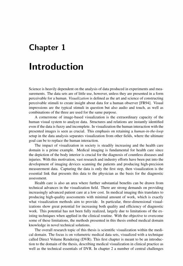
Figure 1.1: An example of a medical data set from CT, a slice from a head scan.
phy (CR) and Direct Radiography (DR), where the x-ray “shadow” of the anatomy isregistered.
The x-ray technique relevant for this thesis is Computed Tomography (CT), pro-ducing volumetric data sets of the patient. The x-ray source and detector are rotatedaround and moved along the patient, measuring the intensity of x-rays passing throughthe body as this spiral progresses. The measurement data are then reconstructed intoattenuation values on a rectilinear 3D grid using an algorithm based on the Radon trans-form. In this case, the tissues do not “shadow” each other, instead, each value describesthe attenuation at a single point in space as seen in figure 1.1.
CT scanners have developed tremendously over the last decade in terms of higherresolution and decreased acquisition time. The most recent development is dual-energyCT, where two different x-ray energies can be used simultaneously, providing moredepiction possibilities. As a result of this progress, there is a strong trend to movemany types of examinations to the CT domain. A drawback of all x-ray techniques isthe dangers of radiation dose, which is limiting the transition to CT.
Magnetic Resonance (MR) imaging is based on a completely different technique.Here the principle of nuclear magnetic resonance is used. A strong magnetic field isused to align the spin of hydrogen nuclei (protons) in the body. Then a radio-frequencypulse matching the nuclear resonance frequency of protons causes the spins to synchro-nize. As the pulse is removed, different relaxation times are measured, i.e., times forthe spins to go out of sync. The measured value depends on the density and chemicalsurrounding of the hydrogen atoms. The spatial localization of each value is controlledby small variations in the magnetic field.
An important distinction from x-ray techniques is that there are in general no knownharmful effects to the patient. MR is, as CT, a volumetric scanning technique. MR isparticularly suitable for imaging of the brain and other soft tissue, where the differenttissues cannot be distinguished well in CT. The noise level is typically higher in MRimages than in the CT case, which for instance causes tissue boundaries to be less
4 CHAPTER 1. INTRODUCTION
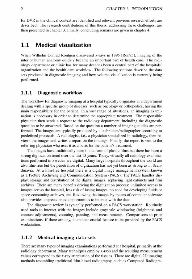
Figure 1.2: An example of a medical data set from MR imaging, a slice from a headscan.
distinct, see figure 1.2. MR methods continue to show tremendous progress and thereis a large set of different examination types that can be performed, such as DiffusionTensor Imaging and Functional MR Imaging.
Ultrasound is another imaging technique without negative side-effects that is widelydeployed. The typical use is for 2D imaging, but there are also 3D scanners. As for CTand MR, ultrasound is continuously finding new application areas. Nuclear imagingalso constitutes an important branch of medical imaging. In contrast to the typical useof other imaging methods, nuclear imaging shows physiological function rather thananatomy, by measuring emission from radioactive substances administered to the pa-tient. Nuclear imaging data sets are typically of low resolution and 3D techniques arecommon, such as Positron Emission Tomography (PET). An important hybrid tech-nique is CT-PET, producing multivariate volumetric data sets of both anatomy andphysiology.
This thesis studies visualization of volumetric data sets and, as described above,there are many sources for medical data of that type. The emphasis in this work is,however, on CT and MR data sets; there will be no examples from ultrasound or nuclearimaging. Many of the above techniques can also produce time-varying data sets but thisis not a focus area in this work. The volumetric data sets are typically formatted as astack of 2D slices when delivered from the scanning modality. The resolution is usuallynot isotropic, i.e., the distance between the slices (the z-direction) is not exactly thesame as the pixel distance within each slice (the x,y-plane). With modern equipment,there is no technical reason for having lower z resolution, but it is often motivated byreduced radiation dose or decreased examination time.
The scale of the produced values motivates some discussion. In CT the valuesdescribe x-ray attenuation that has been calibrated into Hounsfield units (HU), whereair corresponds to -1000 HU and water to 0 HU. This means that a given tissue type
1.1. MEDICAL VISUALIZATION 5
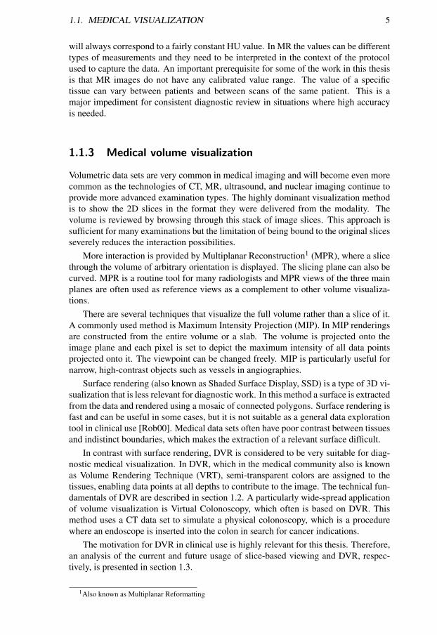
will always correspond to a fairly constant HU value. In MR the values can be differenttypes of measurements and they need to be interpreted in the context of the protocolused to capture the data. An important prerequisite for some of the work in this thesisis that MR images do not have any calibrated value range. The value of a specifictissue can vary between patients and between scans of the same patient. This is amajor impediment for consistent diagnostic review in situations where high accuracyis needed.
1.1.3 Medical volume visualization
Volumetric data sets are very common in medical imaging and will become even morecommon as the technologies of CT, MR, ultrasound, and nuclear imaging continue toprovide more advanced examination types. The highly dominant visualization methodis to show the 2D slices in the format they were delivered from the modality. Thevolume is reviewed by browsing through this stack of image slices. This approach issufficient for many examinations but the limitation of being bound to the original slicesseverely reduces the interaction possibilities.
More interaction is provided by Multiplanar Reconstruction1 (MPR), where a slicethrough the volume of arbitrary orientation is displayed. The slicing plane can also becurved. MPR is a routine tool for many radiologists and MPR views of the three mainplanes are often used as reference views as a complement to other volume visualiza-tions.
There are several techniques that visualize the full volume rather than a slice of it.A commonly used method is Maximum Intensity Projection (MIP). In MIP renderingsare constructed from the entire volume or a slab. The volume is projected onto theimage plane and each pixel is set to depict the maximum intensity of all data pointsprojected onto it. The viewpoint can be changed freely. MIP is particularly useful fornarrow, high-contrast objects such as vessels in angiographies.
Surface rendering (also known as Shaded Surface Display, SSD) is a type of 3D vi-sualization that is less relevant for diagnostic work. In this method a surface is extractedfrom the data and rendered using a mosaic of connected polygons. Surface rendering isfast and can be useful in some cases, but it is not suitable as a general data explorationtool in clinical use [Rob00]. Medical data sets often have poor contrast between tissuesand indistinct boundaries, which makes the extraction of a relevant surface difficult.
In contrast with surface rendering, DVR is considered to be very suitable for diag-nostic medical visualization. In DVR, which in the medical community also is knownas Volume Rendering Technique (VRT), semi-transparent colors are assigned to thetissues, enabling data points at all depths to contribute to the image. The technical fun-damentals of DVR are described in section 1.2. A particularly wide-spread applicationof volume visualization is Virtual Colonoscopy, which often is based on DVR. Thismethod uses a CT data set to simulate a physical colonoscopy, which is a procedurewhere an endoscope is inserted into the colon in search for cancer indications.
The motivation for DVR in clinical use is highly relevant for this thesis. Therefore,an analysis of the current and future usage of slice-based viewing and DVR, respec-tively, is presented in section 1.3.
1Also known as Multiplanar Reformatting
6 CHAPTER 1. INTRODUCTION
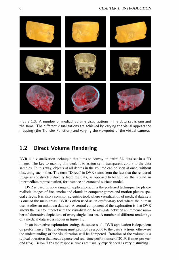
Figure 1.3: A number of medical volume visualizations. The data set is one andthe same. The different visualizations are achieved by varying the visual appearancemapping (the Transfer Function) and varying the viewpoint of the virtual camera.
1.2 Direct Volume Rendering
DVR is a visualization technique that aims to convey an entire 3D data set in a 2Dimage. The key to making this work is to assign semi-transparent colors to the datasamples. In this way, objects at all depths in the volume can be seen at once, withoutobscuring each other. The term “Direct” in DVR stems from the fact that the renderedimage is constructed directly from the data, as opposed to techniques that create anintermediate representation, for instance an extracted surface model.
DVR is used in wide range of applications. It is the preferred technique for photo-realistic images of fire, smoke and clouds in computer games and motion picture spe-cial effects. It is also a common scientific tool, where visualization of medical data setsis one of the main areas. DVR is often used as an exploratory tool where the humanuser studies an unknown data set. A central component of the exploration is that DVRallows the user to interact with the visualization, to navigate between an immense num-ber of alternative depictions of every single data set. A number of different renderingsof a medical data set is shown in figure 1.3.
In an interactive exploration setting, the success of a DVR application is dependenton performance. The rendering must promptly respond to the user’s actions, otherwisethe understanding of the visualization will be hampered. Rotation of the volume is atypical operation that needs a perceived real-time performance of 20-30 frames per sec-ond (fps). Below 5 fps the response times are usually experienced as very disturbing.
1.2. DIRECT VOLUME RENDERING 7
1.2.1 Volumetric data
A volumetric data set, often referred to simply as a volume, is usually considered torepresent a continuous function in a three-dimensional space. Thus, each point in spacecorresponds to a function value, formulated mathematically as:
f : R3→ R
Data sets arising from measurements do not have continuous values, they are lim-ited to the points in space where measurements have been collected. A very commoncase is that the data points constitute a uniform regular grid. Such data points are inthe 3D case known as voxels, a name stemming from their 2D counterpart pixels (pic-ture elements). When values at points in between the original data points are needed,an interpolation between nearby voxels is used as an approximation of the continuousfunction. The voxels do not need to have the same size in all dimensions.
The values in a volumetric data set can represent many different entities and prop-erties. The interpretation of typical medical examinations is given in section 1.1.2.Examples of properties from measurements and simulations in other domains includetemperature, density and electrostatic potential. There can also be more than one valuein each voxel, known as multivariate data, which could be flow velocities and diffusiontensors.
1.2.2 Volume rendering overview
The process of constructing an image from a volumetric data set using DVR can besummarized by the following steps, as defined by Engel et al. [EHK∗06]:
• Data traversal. The positions where samples will be taken from the volume aredetermined.
• Sampling. The data set is sampled at the chosen positions. The sampling pointstypically do not coincide with the grid points, and so interpolation is needed toreconstruct the sample value.
• Gradient computation. The gradient of the data is often needed, in particularas input to the shading component (described below). Gradient computationrequires additional sampling.
• Classification. The sampled values are mapped to optical properties, typicallycolor and opacity. The classification is used to visually distinguish materials inthe volume.
• Shading and illumination. Shading and illumination effects can be used tomodulate the appearance of the samples. The three-dimensional impression isoften enhanced by gradient-based shading.
• Compositing. The pixels of the rendered image are computed by compositingthe optical properties of the samples according to the volume rendering integral.
In the volume rendering process, two parts are particularly central in the trans-formation into a visual representation. The compositing step constitutes the opticalfoundation of the method, and it will be further described in section 1.2.3. The secondcentral part is the classification, representing much of the data exploration in DVR.
8 CHAPTER 1. INTRODUCTION
Classification is typically user-controlled by means of a Transfer Function as describedin section 1.2.4. Further description of the other parts of volume rendering is beyondthe scope of this thesis but they are all active research areas within scientific visualiza-tion, computer graphics, and/or image processing.
The general pipeline components of DVR can be put together in several differentways. There are two main types of methods, image-order and object-order methods.Image-order means that the process originates from the pixels in the image to be ren-dered. Object-order methods approach the process differently – traversing the volumeand projecting partial results onto the screen. The most popular image-order methodis ray casting, where one or more rays are cast through the volume for each pixel inthe image. A very common object-order method is texture slicing, where the volume issampled by a number of 2D slices and then the slices are projected onto the image in thecompositing step. Both ray casting and texture slicing can be effectively implementedon the processing unit of the graphics board, the GPU.
1.2.3 Compositing
The algorithm for creating a volume rendering image is based on simplified models ofthe real physical processes occurring when light interacts with matter. These opticalmodels describe how a ray of light is affected when travelling through the volume.The volume is seen as being composed of different materials that cause absorption andemission of light. Illumination models also include scattering effects, but scatteringwill not be considered in the following for the sake of simplicity. For details beyondthe description below, refer to [EHK∗06].
In the real world, light rays travel through the material and reach the observer,known as the camera in visualization models. When creating an image, each pixel isset to the appearance of a ray ending up in that position. The optical model accountingfor emission and absorption results in the volume rendering integral, that computes thelight reaching the camera:
I(b) = I0 T (a,b)+∫ b
aq(u)T (u,b)du (1.1)
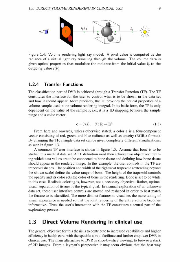
The equation is illustrated in figure 1.4. The ray is defined by entry and exit pointsa and b. The light radiance is given by I, with I(b) being the value at the exit point, i.e.,the image pixel value, and I0 being the light entering from the background. The func-tion T (u,v) is an aggregate of the transparency between points u and v. The functionq(u) specifies the emission at a point along the ray. All in all, the first term accountsfor the absorption of light as the ray passes through the volume and the second termcaptures the emission and color contribution from within the volume, which is alsoaffected by absorption.
Typically, numerical methods are used to compute the volume rendering integral(eq. 1.1) in practice. The ray is divided into n small segments, for which the opticalproperties are assumed to be approximately constant. The emission contribution from asegment i then becomes a single color ci. The transparency Ti is usually denoted by theopposite property opacity, αi = 1−Ti. The resulting radiance I(b) = ctot is typicallycomputed iteratively from front to back, from b to a:
ctot ← ctot +(1−αtot) ·αi · ci
αtot ← αtot +(1−αtot) ·αi
}i = n,n−1, . . . ,1 (1.2)
1.3. DIRECT VOLUME RENDERING IN CLINICAL USE 9
I(b)b a
I0
Figure 1.4: Volume rendering light ray model. A pixel value is computed as theradiance of a virtual light ray travelling through the volume. The volume data isgiven optical properties that modulate the radiance from the initial value I0 to theoutgoing value I(b).
1.2.4 Transfer Functions
The classification part of DVR is achieved through a Transfer Function (TF). The TFconstitutes the interface for the user to control what is to be shown in the data setand how it should appear. More precisely, the TF provides the optical properties of avolume sample used in the volume rendering integral. In its basic form, the TF is onlydependent on the value of the sample s, i.e., it is a 1D mapping between the samplerange and a color vector:
c = T(s), T : R→ R4 (1.3)
From here and onwards, unless otherwise stated, a color c is a four-componentvector consisting of red, green, and blue radiance as well as opacity (RGBα format).By changing the TF, a single data set can be given completely different visualizations,as seen in figure 1.3.
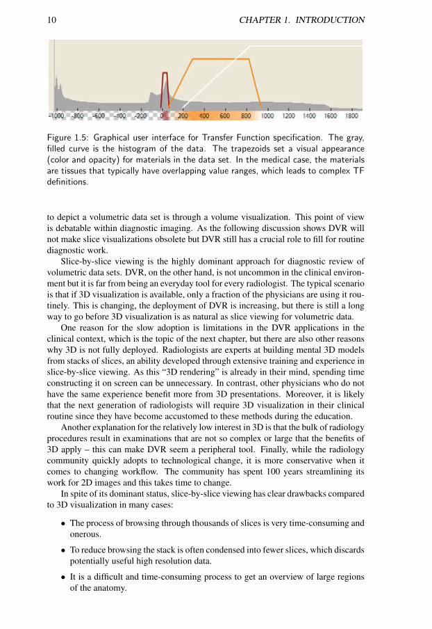
A common TF user interface is shown in figure 1.5. Assume that bone is to bestudied in a medical data set. A TF definition must then achieve two objectives: defin-ing which data values are to be connected to bone tissue and defining how bone tissueshould appear in the rendered image. In this example, the user controls in the TF aretrapezoid shapes. The position and width of the rightmost trapezoid (extending beyondthe shown scale) define the value range of bone. The height of the trapezoid controlsthe opacity and its color sets the color of bone in the rendering. Bone is set to be whitein this case. Realistic coloring is, however, not a necessary objective. Rather, optimalvisual separation of tissues is the typical goal. In manual exploration of an unknowndata set, these user interface controls are moved and reshaped in order to best matchthe feature to be classified. The more distinct features to visualize, the more tuning ofvisual appearance is needed so that the joint rendering of the entire volume becomesinformative. Thus, the user’s interaction with the TF constitutes a central part of theexploratory process.
1.3 Direct Volume Rendering in clinical use
The general objective for this thesis is to contribute to increased capabilities and higherefficiency in health care, with the specific aim to facilitate and further empower DVR inclinical use. The main alternative to DVR is slice-by-slice viewing; to browse a stackof 2D images. From a layman’s perspective it may seem obvious that the best way
10 CHAPTER 1. INTRODUCTION
Figure 1.5: Graphical user interface for Transfer Function specification. The gray,filled curve is the histogram of the data. The trapezoids set a visual appearance(color and opacity) for materials in the data set. In the medical case, the materialsare tissues that typically have overlapping value ranges, which leads to complex TFdefinitions.
to depict a volumetric data set is through a volume visualization. This point of viewis debatable within diagnostic imaging. As the following discussion shows DVR willnot make slice visualizations obsolete but DVR still has a crucial role to fill for routinediagnostic work.
Slice-by-slice viewing is the highly dominant approach for diagnostic review ofvolumetric data sets. DVR, on the other hand, is not uncommon in the clinical environ-ment but it is far from being an everyday tool for every radiologist. The typical scenariois that if 3D visualization is available, only a fraction of the physicians are using it rou-tinely. This is changing, the deployment of DVR is increasing, but there is still a longway to go before 3D visualization is as natural as slice viewing for volumetric data.
One reason for the slow adoption is limitations in the DVR applications in theclinical context, which is the topic of the next chapter, but there are also other reasonswhy 3D is not fully deployed. Radiologists are experts at building mental 3D modelsfrom stacks of slices, an ability developed through extensive training and experience inslice-by-slice viewing. As this “3D rendering” is already in their mind, spending timeconstructing it on screen can be unnecessary. In contrast, other physicians who do nothave the same experience benefit more from 3D presentations. Moreover, it is likelythat the next generation of radiologists will require 3D visualization in their clinicalroutine since they have become accustomed to these methods during the education.
Another explanation for the relatively low interest in 3D is that the bulk of radiologyprocedures result in examinations that are not so complex or large that the benefits of3D apply – this can make DVR seem a peripheral tool. Finally, while the radiologycommunity quickly adopts to technological change, it is more conservative when itcomes to changing workflow. The community has spent 100 years streamlining itswork for 2D images and this takes time to change.
In spite of its dominant status, slice-by-slice viewing has clear drawbacks comparedto 3D visualization in many cases:
• The process of browsing through thousands of slices is very time-consuming andonerous.
• To reduce browsing the stack is often condensed into fewer slices, which discardspotentially useful high resolution data.
• It is a difficult and time-consuming process to get an overview of large regionsof the anatomy.
1.4. CONTRIBUTIONS 11
• It is difficult to perceive complex structures extending orthogonally to the sliceplane, e.g., vessel trees.
• The understanding of non-radiologists reviewing the images is hampered.
The most driving factor for DVR deployment will be the continuous increase indata set sizes. Even the radiologists that prefer traditional slice viewing will need DVRfor overview and navigation.
The conclusion to be drawn is that slice visualization suffers from limitations thatare increasingly problematic. In light of the additional capabilities provided, DVRis a necessary complement in diagnostic imaging. In order to achieve the requireddeployment of DVR in clinical use, there a number of challenges to be met. Some ofthe major obstacles to overcome are presented in the next chapter.
1.4 Contributions
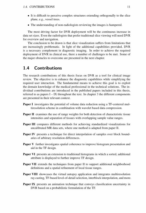
The research contributions of this thesis focus on DVR as a tool for clinical imagereview. The objective is to enhance the diagnostic capabilities while simplifying therequired user interaction. The fundamental means to achieve this goal is to exploitthe domain knowledge of the medical professional in the technical solutions. The in-dividual contributions are introduced in the published papers included in this thesis,referred to as papers I – IX throughout the text. In chapter 3 the different componentsare presented in their relevant context.
Paper I investigates the potential of volume data reduction using a TF-centered mul-tiresolution scheme in combination with wavelet based data compression.
Paper II examines the use of range weights for both detection of characteristic tissueintensities and separation of tissues with overlapping sample value ranges.
Paper III compares different methods for achieving standardized visualizations foruncalibrated MR data sets, where one method is adapted from paper II.
Paper IV presents a technique for direct interpolation of samples over block bound-aries of arbitrary resolution differences.
Paper V further investigates spatial coherence to improve histogram presentation andaid in the TF design.
Paper VI presents an extension to traditional histograms in which a sorted, additionalattribute is displayed to further improve TF design.
Paper VII extends the techniques from paper II to support additional neighborhooddefinitions and a spatial refinement of local tissue ranges.
Paper VIII showcases the virtual autopsy application and integrates multiresolutionray casting, TF-based level-of-detail selection, interblock interpolation, and more.
Paper IX presents an animation technique that conveys classification uncertainty inDVR based on a probabilistic formulation of the TF.

12 CHAPTER 1. INTRODUCTION
Chapter 2
Challenges inMedical Volume Rendering
Direct Volume Rendering is a technique that offers many potential benefits to diagnos-tic work within medical imaging, as described in the previous chapter. DVR enablesanalysis of more complex cases than before, while being more efficient and allowingmore accurate assessments for certain standard examinations. The work presented inthis thesis aims to address some of the specific challenges that DVR needs to meet inthe clinical context. These challenges are described in-depth in this chapter along withan overview of previous research efforts in this field.
2.1 Large data sets
There has been a rapid technical development of medical imaging modalities in re-cent years, which has enabled important benefits for the diagnostic methods. Signifi-cantly improved spatial resolution of the data sets has enabled more detailed diagnosticassessments and multivariate measurements lead to unprecedented analysis possibil-ities. Furthermore, the decreased scan times allow procedures that were previouslyimpossible, for instance high-quality scans of beating hearts. The drawback of thisimportant progress is an enormous increase in data set sizes, even for routine examina-tions [And03].
Conventional technical solutions have not been sufficient to deal with the contin-uously growing data sizes. For visualization techniques in general, and DVR in par-ticular, there is an urgent need for improved methods in order to achieve interactiveexploration of the data sets. One aspect is the technical limitations in terms of mem-ory capacity and bandwidth that pose serious challenges for the visualization pipeline,making sufficiently high frame rates hard to reach. To achieve the performance neededfor DVR in clinical use, methods that can reduce the memory and bandwidth require-ments for retrieval, unpacking and rendering of the large data sets must be developed.
There is also a human aspect of the large data set problem. The gigabytes of avail-able data is neither possible nor necessary for the physician to take in. A mere fewkilobytes may be enough for the assessment task being addressed, which entails thatthe task of the visualization is to assist in finding this small subset in an efficient way.The objective of medical visualization is thus transforming from displaying all avail-able data to navigating within the data.
14 CHAPTER 2. CHALLENGES IN MEDICAL VOLUME RENDERING
Capture Storage Visualization
Dynamic data
reduction
Data relevance
Static data
reduction
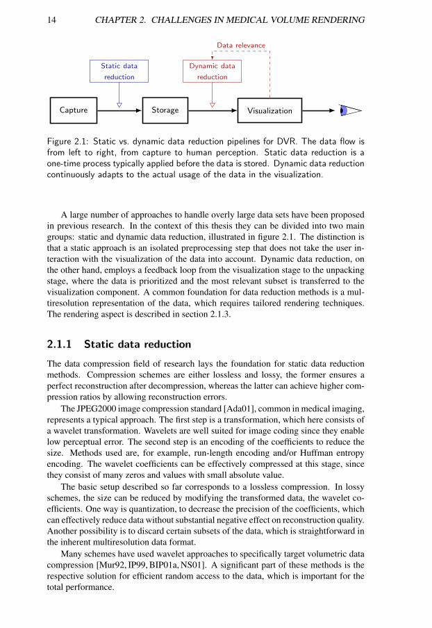
Figure 2.1: Static vs. dynamic data reduction pipelines for DVR. The data flow isfrom left to right, from capture to human perception. Static data reduction is aone-time process typically applied before the data is stored. Dynamic data reductioncontinuously adapts to the actual usage of the data in the visualization.
A large number of approaches to handle overly large data sets have been proposedin previous research. In the context of this thesis they can be divided into two maingroups: static and dynamic data reduction, illustrated in figure 2.1. The distinction isthat a static approach is an isolated preprocessing step that does not take the user in-teraction with the visualization of the data into account. Dynamic data reduction, onthe other hand, employs a feedback loop from the visualization stage to the unpackingstage, where the data is prioritized and the most relevant subset is transferred to thevisualization component. A common foundation for data reduction methods is a mul-tiresolution representation of the data, which requires tailored rendering techniques.The rendering aspect is described in section 2.1.3.
2.1.1 Static data reduction
The data compression field of research lays the foundation for static data reductionmethods. Compression schemes are either lossless and lossy, the former ensures aperfect reconstruction after decompression, whereas the latter can achieve higher com-pression ratios by allowing reconstruction errors.
The JPEG2000 image compression standard [Ada01], common in medical imaging,represents a typical approach. The first step is a transformation, which here consists ofa wavelet transformation. Wavelets are well suited for image coding since they enablelow perceptual error. The second step is an encoding of the coefficients to reduce thesize. Methods used are, for example, run-length encoding and/or Huffman entropyencoding. The wavelet coefficients can be effectively compressed at this stage, sincethey consist of many zeros and values with small absolute value.
The basic setup described so far corresponds to a lossless compression. In lossyschemes, the size can be reduced by modifying the transformed data, the wavelet co-efficients. One way is quantization, to decrease the precision of the coefficients, whichcan effectively reduce data without substantial negative effect on reconstruction quality.Another possibility is to discard certain subsets of the data, which is straightforward inthe inherent multiresolution data format.
Many schemes have used wavelet approaches to specifically target volumetric datacompression [Mur92, IP99, BIP01a, NS01]. A significant part of these methods is therespective solution for efficient random access to the data, which is important for thetotal performance.
2.1. LARGE DATA SETS 15
The Discrete Cosine Transform (DCT) is another transformation used in a similartwo-step setup. It is the base of the original JPEG codec [ITU92]. Also DCT has beenapplied to volumetric data compression [YL95, PW03].
A third class of compression methods is vector quantization [NH92], resulting inlossy compression. This method operates on multidimensional vectors, which typi-cally are constructed from groups of data samples. The vector space is quantized, i.e.,reduced to a finite set of model vectors. An arbitrary input vector is approximated byone of the quantized vectors, which allows for efficient subsequent encoding. Vec-tor quantization can also be combined with other approaches, by letting it operate ontransformed coefficients [SW03].
An important part of the compression algorithms described above is that they em-ploy blocking in some form. Blocking is a subdivision of the data set into small regions,known as blocks or bricks, which are processed individually. The appropriate choiceof block size depends heavily on the characteristics of the hardware components of thecomputer system in use.
The standard compression methods have been extended for visualization purposes.Bajaj et al. [BIP01b] introduce voxel visualization importance as a weight factor ina wavelet compression approach. Coefficients corresponding to important voxels areprioritized, resulting in higher visual quality in the subsequently rendered image. In asimilar approach, Sohn et al. [SBS02] let volumetric features guide the compression,in their case applied to time-varying volumes. A significant drawback with both theseapproaches is that the important features need to be known at compression time.
A combined compression and rendering scheme for DVR based on vector quan-tization was proposed by Schneider and Westermann [SW03]. An advantage of thisapproach is the ability to both decompress and render on the graphics hardware. Anexample of data reduction for irregular volumetric data is the work of Cignoni etal. [CMPS97]. In this case, compression corresponds to topology-preserving simplifi-cation of a tetrahedral mesh.
An important point that sometimes is overseen is that the data reduction should beretained throughout the pipeline, even at the rendering stage. In a traditional pipelinesetup, the decompression algorithm restores the data to full resolution even if the qual-ity is lower. This means that the full amount of data must be handled in the rendering,thus disabling the data reduction effect that would be highly desired to increase render-ing performance and decrease the need for GPU memory.
Furthermore, it is necessary to bear in mind that maximal compression ratio doesnot necessarily mean maximal performance. The overall performance of the entirepipeline should be considered and one crucial factor is the decompression speed. Thealgorithm providing the best compression ratio may be an inappropriate choice if thedecompression is slow. Depending on the system characteristics, it may be better toavoid compression altogether if the decrease in transfer time is exceeded by the increasein processing time.
2.1.2 Dynamic data reduction
Dynamic data reduction methods go one step further compared to the standard notionof compression. The idea is that visualization parameters, which in DVR could bethe distance to the camera, the Transfer Function (TF), the viewpoint, etc., entails thatthe demand on precision varies substantially within the data set. Thus, the data canbe reduced in these regions, without much loss in the quality of the rendered image.The key feature of a dynamic method is the ability to adapt to changing parameters,
16 CHAPTER 2. CHALLENGES IN MEDICAL VOLUME RENDERING
by way of a feed-back loop from the rendering to the unpacking/decompression stage,as illustrated in figure 2.1. In contrast, static data reduction methods are not adaptivesince they are defined once and for all at compression time.
A number of volume rendering pipelines employing dynamic data reduction havebeen developed. Several multiresolution DVR schemes have been proposed that em-ploy an level-of-detail (LOD) selection based on, for example, distance to viewpointand field-of-view size [LHJ99, WWH∗00, BNS01]. A full visualization pipeline waspresented by Guthe et al. [GWGS02] where a multiresolution representation is achievedthrough a blocked wavelet compression scheme. An LOD selection is performed at thedecompression stage, prioritizing block resolution according to the distance to view-point and the L2 data error of the resolution level. Gao et al. [GHJA05] presented LODselection based on TF-transformed data computed using a coarse value histogram. Allthe above methods are based on an octree structure, i.e., a hierarchical recursive sub-division with increasing resolution. As shown by Ljung [Lju06b], a straightforwardflat blocking scheme is a more compact representation for data with abrupt changes inresolution levels.
An important part of a multiresolution scheme is to accurately estimate the im-pact a lower LOD would have on the rendered image quality. A main challenge is toaccurately incorporate the effect of TF transformation without introducing extensiveoverhead. Furthermore, the method needs to adapt to interactive changes to the TF.Dedicated efforts to estimate LOD impact have been made. One approach is to tabulatethe frequency of each actual value distortion and compute the impact after applying theTF [LHJ03], but the size of such tables is feasible only for 8-bit data. Other approachesinclude a conservative but reasonably fast approximation of actual screen-space errorin a multiresolution DVR scheme [GS04] and a computation of block transparencyacross all viewpoints used for visibility culling [GHSK03].
The research contributions in this thesis include a volume rendering pipeline basedon the principles of dynamic data reduction but also allowing static data reduction. Thepipeline, presented in section 3.1, combines a TF-based LOD selection with a waveletcompression scheme.
2.1.3 Multiresolution DVR
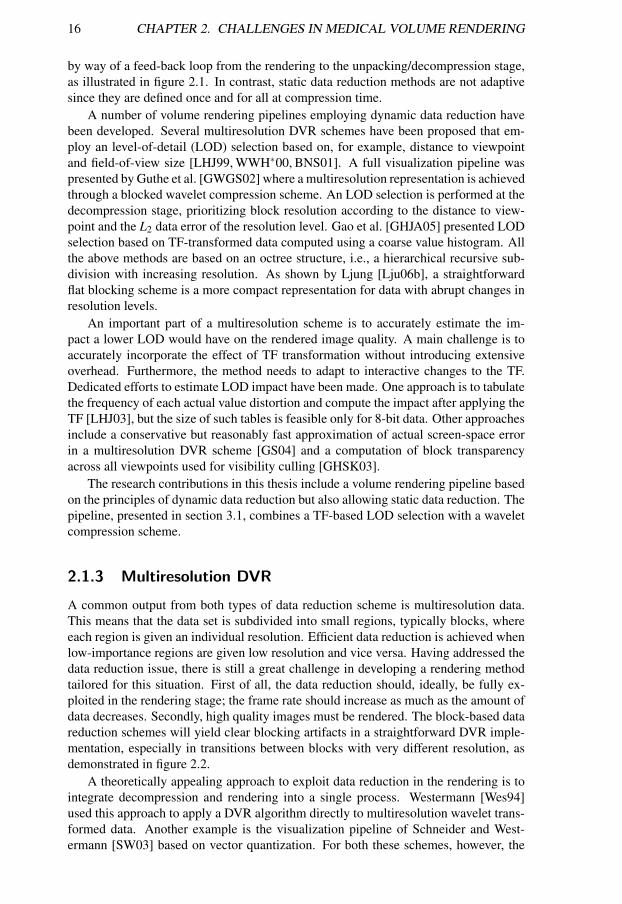
A common output from both types of data reduction scheme is multiresolution data.This means that the data set is subdivided into small regions, typically blocks, whereeach region is given an individual resolution. Efficient data reduction is achieved whenlow-importance regions are given low resolution and vice versa. Having addressed thedata reduction issue, there is still a great challenge in developing a rendering methodtailored for this situation. First of all, the data reduction should, ideally, be fully ex-ploited in the rendering stage; the frame rate should increase as much as the amount ofdata decreases. Secondly, high quality images must be rendered. The block-based datareduction schemes will yield clear blocking artifacts in a straightforward DVR imple-mentation, especially in transitions between blocks with very different resolution, asdemonstrated in figure 2.2.
A theoretically appealing approach to exploit data reduction in the rendering is tointegrate decompression and rendering into a single process. Westermann [Wes94]used this approach to apply a DVR algorithm directly to multiresolution wavelet trans-formed data. Another example is the visualization pipeline of Schneider and West-ermann [SW03] based on vector quantization. For both these schemes, however, the
2.2. INTERACTIVE TISSUE CLASSIFICATION 17
Figure 2.2: Example of blocking artifacts in multiresolution DVR. Left, middle: Orig-inal rendering. Right: Multiresolution rendering with high data reduction showinga clear block structure.
additional complexity of the rendering prevents performance benefits from the reducedmemory footprint.
The image quality issue in multiresolution DVR has been addressed in GPU-basedschemes. LaMar et al. [LHJ99] proposed a multiresolution rendering approach withblock-independent processing, where a spherical shell geometry reduces the interblockartifacts. A drawback of the block-independent approach is that it does not provide acontinuous transition between blocks. Therefore, data set subdivisions with overlap-ping blocks have been developed [WWH∗00,GWGS02]. Lower resolution samples arereplicated at boundaries to higher resolution blocks in order to handle discontinuities.An unwanted side effect is that replication counteracts the data reduction.
The multiresolution DVR pipeline presented in this thesis addresses the issue ofblocking artifacts through an interblock interpolation scheme. Without resorting tosample replication, the scheme achieves smooth block transitions, as presented in sec-tion 3.1.4.
2.2 Interactive tissue classification
The work of reviewing medical images corresponds, to a great extent, to identifyingand delineating different tissues. If this classification is performed correctly, drawingthe diagnostic conclusions is often a straightforward task for the trained professional.In the current context, the classification process can be defined as analyzing each voxelwith respect to a set of tissues, and for each tissue determining the probability that thevoxel belongs to it.
There is an important distinction in what kind of problem a classification scheme at-tempts to solve. Image processing often deals with precise segmentations where quan-titative measurements are a typical objective. The focus in this thesis is the scientificvisualization approach, where the classification method is a tool for interactive explo-ration of the data. In this case, the qualitative aspect of the outcome is more importantand an intuitive and direct connection between user and machine is crucial. Thesecharacteristics are not common for existing classification and segmentation schemes.
Another relevant grouping of methods is into specialized and general approaches.If the classification is restricted to a narrow domain, good results can be achieved evenby fairly automated methods. Examples include the bronchi segmentation of Bartzet al. [BMF∗03] and the hip joint segmentation of Zoroofi et al. [ZSS∗03]. A differentchallenge is to create general methods that work for a wide range of image types, whichis the objective of the DVR methods presented in this thesis.
18 CHAPTER 2. CHALLENGES IN MEDICAL VOLUME RENDERING
2.2.1 One-dimensional Transfer Functions
Medical images have been used for more than a century and for most of that time thediagnostic work flow has been streamlined for the classical x-ray image. One aspect ofthis is that a scalar value (for example, x-ray attenuation or signal intensity) is by far themost common tissue classification domain. In the DVR context, such a classificationcorresponds to a 1D TF as described in section 1.2.4.
The 1D TF is, however, not sufficient for the diagnostic tasks of a modern radiol-ogist. Many tissues cannot be separated using only the scalar value; in virtually everyexamination, the different tissues have fully or partly overlapping value ranges. Thisis true for nearly every MR data set and for CT data sets in the case of distinguishingdifferent soft tissues. The typical remedy when tissue separation is needed, is to ad-minister contrast agent to the patient before or during the scan. This is very effectivewhen a suitable contrast agent exists, but many diagnostic cases are not yet covered.Furthermore, even data sets with contrast agent can pose problems for DVR. One rea-son is that new range overlap occurs, as in CT angiographies where blood vessels withcontrast agent have the same attenuation as spongy bone. Another common situation isthat the differences between the tissues are too subtle to be studied in DVR, for exam-ple tumor tissue vs. liver parenchyma in CT examinations. In these cases, informativevolume rendering images from 1D TFs are impossible to obtain and the visualizationis limited to 2D slices.
In spite of the limitations, the 1D TF is the most important classification interfacefor the human user. This has been the case ever since the initial DVR method proposedby Drebin et al. [DCH88], where such a one-dimensional mapping is employed. Anoverview of usability aspects for 1D TF design was presented by Konig [Kon01]. Inmany commercial applications for medical DVR, the TF user interface consists of wid-gets controlling a direct mapping from data value ranges to rgbα vectors. Wheneverfurther tissue separation is needed the user needs to resort to manual sculpting, cuttingaway disturbing regions of the volume.
2.2.2 Multidimensional Transfer Functions
Many research efforts have been targeted towards overcoming the classification limita-tions of 1D TFs. A common approach has been to add dimensions to the TF domain,primarily in order to capture boundary characteristics. Two-dimensional TFs using gra-dient magnitude as the additional dimension were introduced by Levoy [Lev88]. Exten-sions to this method to further empower classification connected to material boundarieshave been proposed over the years [KD98, RBS05, SVSG06].
Apart from capturing pure boundary information, measures of local structure com-puted from second order derivatives have been employed for classification purposes[SWB∗00]. For material separation within volumetric surfaces, curvature-based TFshave been shown to add visualization possibilities by conveying shape characteris-tics [HKG00, KWTM03].
The multidimensional TF schemes above have benefits in the form of enhancedvisualization of material boundaries. These solutions are, however, not sufficient inthe medical case. One reason is that the boundaries are often far from distinct dueto inherent noise [PBSK00]. Even when there are well defined boundaries betweentissues, the interior properties of a tissue is often diagnostically important. Moreover,it is not uncommon that separation of unstructured tissues of similar intensity is needed,which is a situation that neither structure nor boundary approaches can handle.
2.3. TISSUE DETECTION 19
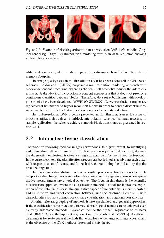
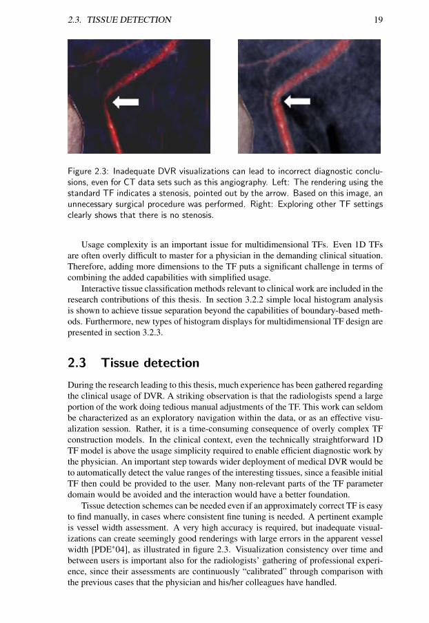
Figure 2.3: Inadequate DVR visualizations can lead to incorrect diagnostic conclu-sions, even for CT data sets such as this angiography. Left: The rendering using thestandard TF indicates a stenosis, pointed out by the arrow. Based on this image, anunnecessary surgical procedure was performed. Right: Exploring other TF settingsclearly shows that there is no stenosis.
Usage complexity is an important issue for multidimensional TFs. Even 1D TFsare often overly difficult to master for a physician in the demanding clinical situation.Therefore, adding more dimensions to the TF puts a significant challenge in terms ofcombining the added capabilities with simplified usage.
Interactive tissue classification methods relevant to clinical work are included in theresearch contributions of this thesis. In section 3.2.2 simple local histogram analysisis shown to achieve tissue separation beyond the capabilities of boundary-based meth-ods. Furthermore, new types of histogram displays for multidimensional TF design arepresented in section 3.2.3.
2.3 Tissue detection
During the research leading to this thesis, much experience has been gathered regardingthe clinical usage of DVR. A striking observation is that the radiologists spend a largeportion of the work doing tedious manual adjustments of the TF. This work can seldombe characterized as an exploratory navigation within the data, or as an effective visu-alization session. Rather, it is a time-consuming consequence of overly complex TFconstruction models. In the clinical context, even the technically straightforward 1DTF model is above the usage simplicity required to enable efficient diagnostic work bythe physician. An important step towards wider deployment of medical DVR would beto automatically detect the value ranges of the interesting tissues, since a feasible initialTF then could be provided to the user. Many non-relevant parts of the TF parameterdomain would be avoided and the interaction would have a better foundation.
Tissue detection schemes can be needed even if an approximately correct TF is easyto find manually, in cases where consistent fine tuning is needed. A pertinent exampleis vessel width assessment. A very high accuracy is required, but inadequate visual-izations can create seemingly good renderings with large errors in the apparent vesselwidth [PDE∗04], as illustrated in figure 2.3. Visualization consistency over time andbetween users is important also for the radiologists’ gathering of professional experi-ence, since their assessments are continuously “calibrated” through comparison withthe previous cases that the physician and his/her colleagues have handled.
20 CHAPTER 2. CHALLENGES IN MEDICAL VOLUME RENDERING
2.3.1 Unsupervised tissue identification
There are an immense number of classification approaches that could be used for sub-sequent TF design. As noted in section 2.2, however, there exists a great challengein developing generally applicable methods. The most common tissue identificationmethod in DVR is to display the full data set histogram to the user; the idea beingthat the relevant tissues will stand out as peaks in the histogram. Unfortunately, thisis seldom the case, which makes the global histogram a very blunt tool for accuratedefinition of tissue value ranges.
Some research efforts have been made to find general methods that can be usedto predict suitable visualization parameters. Bajaj et al. [BPS97] introduced metricsfor identifying appropriate values for isosurface rendering of triangular meshes, theContour Spectrum. A similar method targeting regular cartesian data has also beendeveloped [PWH01].
Tissue detection is particularly important for MR image volumes because of theuncalibrated scale of the voxel values. Previous research efforts have targeted auto-matic adaptation of visualization parameters for MR data sets [NU99, Oth06]. Theadaptations are based on landmarks of the shape of the global histogram. A limitationis that these methods are only applicable for examination types where the global his-togram shape is consistent between patients. Rezk-Salama et al. [RSHSG00] use bothhistograms and boundary measures to adapt TF settings between data sets.
Two different histogram analysis techniques addressing the tissue detection chal-lenge are presented in section 3.3 of this thesis. Both techniques exploit spatial relationsin the data to enhance the value of histogram presentations.
2.3.2 Simplified TF design
Many research efforts aim to simplify the manual interaction in TF construction with-out using automatic tissue detection. In traditional TF specification, the user interac-tion is directly connected to the volumetric data set, this is known as the data-drivenapproach. Within this class of methods Kindlmann and Durkin [KD98] suggested asimplification of parameters for boundary visualization in DVR where the user definesa mapping between surface distance and opacity. Extensions to this model have beenproposed [TLM01, KKH02]. There are also more general data exploration interfacesthat are not limited to boundary measures [PBM05].
Another way to simplify traditional TF specification is data probing, i.e., to let theuser select representative points or regions in the data set as base for the TF param-eters. A data probe is part of the tools presented by Kniss et al. [KKH02]. In theDVR approach of Tzeng et al. [TLM03] probing is used to drive a high-dimensionalclassification based on an artificial neural network.
With the aim to create a more intuitive 2D TF interface, Rezk-Salama et al. [RSKK06]developed a framework based on a user-oriented semantic abstraction of the parame-ters. A Principal Component Analysis approach is employed to reduce the TF interac-tion space.
In contrast with data-driven methods, image-driven methods let the user adjust thevisualization by selecting from alternative rendered images, changing the TF in anindirect way. The challenge is then to automatically provide the user with a relevantgallery of different settings. He et al. [HHKP96] explore stochastic generation of thesealternatives. Further variants and extensions of gallery schemes have been proposed[MAB∗97, KG01].
2.4. UNCERTAINTY VISUALIZATION 21
2.4 Uncertainty visualization
The challenge of representing errors and uncertainty in visualization applications hasbeen brought forward as one of the main topics for future visualization research [JS03,Joh04]. The benefit of controlling and studying the uncertainty is highly valid withinmedical DVR. An important aspect is the uncertainty that the user introduces by settingthe visualization parameters. A static TF yields a certain appearance in the renderedimage, but it is very important that the user can explore the robustness of this settingto make sure that the diagnostic conclusion is not affected by slight mistakes in theTF definition. Figure 2.3 above shows a real-life example of the patient safety risksinvolved.
In fact, the TF uncertainty is today often assessed by the radiologists through man-ual adjustments back and forth. A main drawback is that this is very time-consuming.Moreover, the full parameter space relevant to the diagnosis may not be covered by thead-hoc manual adjustments. This problem grows with the complexity of the TFs used.All in all, there is a substantial risk, especially for physicians with limited DVR expe-rience, that this manual process deviates far from the ideal: an unbiased exploration ofall relevant possibilities.
2.4.1 Uncertainty types
A thorough survey of many aspects of uncertainty visualization was presented by Panget al. [PWL97]. A taxonomy of different methods was proposed, as well as a cate-gorization of uncertainty sources into three groups: acquisition, transformation, andvisualization. In the first category statistical variations due to measurement error orsimulation simplifications are typical examples. Transformation uncertainty is exem-plified by resampling and quantization of data values. Finally, approximations areintroduced in the visualization scheme which for instance is manifested by the fact thatdifferent DVR schemes do not result in the exact same rendering of a volume.
This thesis focuses on uncertainty arising from the TFs fuzzy classification withinDVR, which belongs to the “visualization uncertainty” group. An important distinctionis that many previous methods have assumed that the probability values are derived ormeasured before the visualization stage occurs, whereas the current focus is statisticalvariation inherent in the visualization process.
2.4.2 Visual uncertainty representations
A number of methods have aimed at representing uncertainty in surface visualizations.The survey of Pang et al. [PWL97] presented several uncertainty representations forsurface renderings and proposed additional schemes. One possibility is to connectuncertainty to a proportional spatial displacement of the surface, resulting in a pointcloud appearance for low-confidence regions [GR04]. Without changing the spatialextent of the surface, variations in the appearance can be used to convey uncertainty.Hue and texture have been used to visualize isosurface confidence in multiresolutiondata [RLBS03]. Furthermore, flowline curvature has been employed to represent shapeuncertainty of an isosurface [KWTM03].
It is difficult to extend the above surface rendering methods to the volume renderingcase. Other researchers have focused on DVR-specific solutions, proposing differentways to incorporate volumetric probabilities. A straightforward solution is to treat
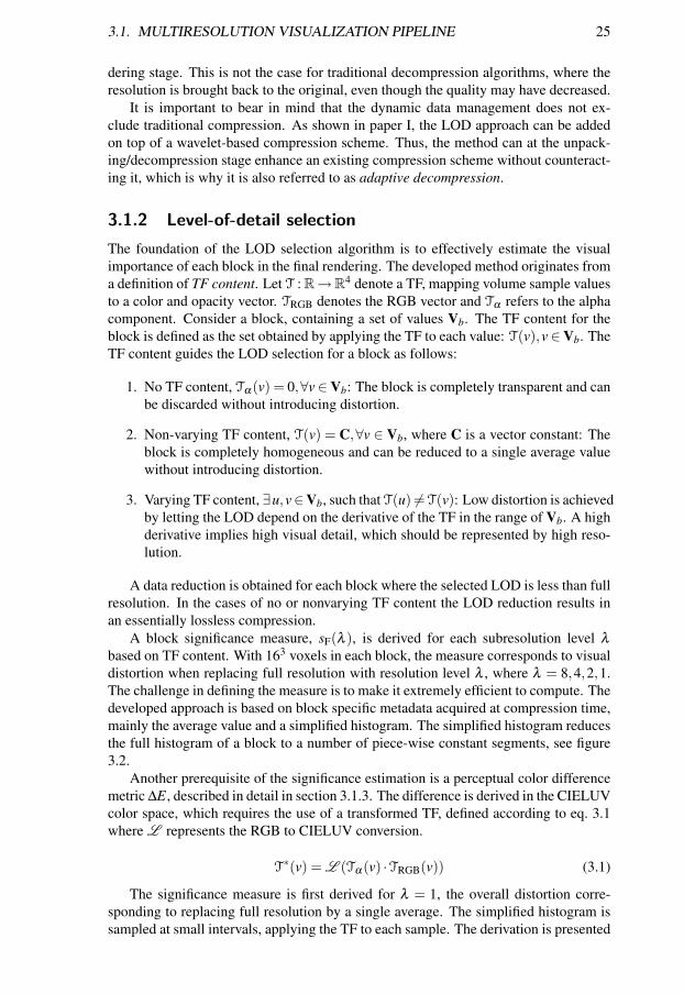
22 CHAPTER 2. CHALLENGES IN MEDICAL VOLUME RENDERING
these likelihood values as any other attribute to be visualized, either rendering the like-lihood domain itself [RJ99] or applying a multidimensional TF [DKLP01]. In anotherapproach the probability volume is rendered and then used to modulate the pixels of therendering of the data volume [DKLP01]. A serious limitation of this last approach isthat there is no correlation of obscured regions in the two renderings; uncertain regionsmay affect the final result even if they are not visible in the regular rendering.
The task of visualizing uncertainty from a predefined probabilistic classificationwas addressed by Kniss et al. [KUS∗05], proposing a DVR framework based on sta-tistical risk. The methods include a graph-based data reduction scheme to deal withthe challenge of the enlargement of the data sets resulting from the transformation tomaterial classification volumes.
Uncertainty can also be represented by controlled changes in the rendered image.There are examples of such animation schemes in the area of geographical visualiza-tion. Gershon [Ger92] used an ordered set of segmentations, which was animated inorder to make fuzzy structures stand out. The method of Ehlschlaeger et al. [ESG97]creates a sequence of probabilistically derived rendering realizations to convey spatialuncertainty.
The final research contribution in this thesis is an uncertainty animation techniquetailored for clinical use, presented in section 3.4. The foundation is a probabilisticinterpretation of the TF, that may become useful also for DVR in general.
Chapter 3
Efficient Medical VolumeVisualization
Based on vast research efforts over the past decades both performance and quality ofvolume visualization have continuously been improved. Medical imaging has been,and is, a prime application area for the developed methods. Despite its success in med-ical research, volume visualization approaches have not had the same impact in routineclinical situations. To find the reason for this it is important to realize that the needsof a practicing radiologist reading hundreds of examinations per day are not the sameas those of a medical researcher, who can spend significant amount of time analyzingindividual cases. To reach a more wide-spread use outside of the research field it isthus crucial to work in continuous close collaboration with medical professionals andthe medical visualization industry to gain an understanding of the issues involved inthe user’s clinical workflow.
This chapter describes the research contributions found in the appended papersand puts these contributions in the context of the challenges described in the previouschapter. A main theme of the work is that the clinical usage is put at the core of theresearch methodology. The common foundation of the developed methods is thus thatthey are based on the clinical visualization user’s perspective and exploit the availablemedical domain knowledge to address identified pertinent problems. The presentationwill show that these methods tailored for the clinical context can lead to increasedperformance and enhanced quality, thereby increasing the user’s ability to fulfill thetask at hand.
3.1 Multiresolution visualization pipeline
The first of the identified challenges for DVR in clinical use is the increasingly largedata sets, as discussed in section 2.1. With the objective to deal with central partsof this challenge and lay a foundation for future research efforts, a multiresolutionDVR pipeline has been developed. The presentation of the pipeline in this sectioncorresponds to papers I, IV and VIII.
The goal is to significantly reduce the amount of data to be processed throughouta Direct Volume Rendering (DVR) pipeline. The path taken in this thesis puts theTransfer Function (TF) at the core, exploiting the user’s definition of what to makevisible in the data set. When applying a TF large subsets of the volume will give little
24 CHAPTER 3. EFFICIENT MEDICAL VOLUME VISUALIZATION
Capture Packing Storage Unpacking Rendering
TF, viewpointBlocking Compression
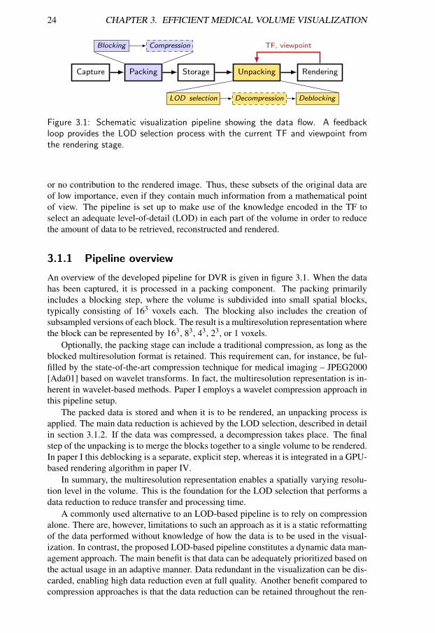
LOD selection Decompression Deblocking
Figure 3.1: Schematic visualization pipeline showing the data flow. A feedbackloop provides the LOD selection process with the current TF and viewpoint fromthe rendering stage.
or no contribution to the rendered image. Thus, these subsets of the original data areof low importance, even if they contain much information from a mathematical pointof view. The pipeline is set up to make use of the knowledge encoded in the TF toselect an adequate level-of-detail (LOD) in each part of the volume in order to reducethe amount of data to be retrieved, reconstructed and rendered.
3.1.1 Pipeline overview
An overview of the developed pipeline for DVR is given in figure 3.1. When the datahas been captured, it is processed in a packing component. The packing primarilyincludes a blocking step, where the volume is subdivided into small spatial blocks,typically consisting of 163 voxels each. The blocking also includes the creation ofsubsampled versions of each block. The result is a multiresolution representation wherethe block can be represented by 163, 83, 43, 23, or 1 voxels.
Optionally, the packing stage can include a traditional compression, as long as theblocked multiresolution format is retained. This requirement can, for instance, be ful-filled by the state-of-the-art compression technique for medical imaging – JPEG2000[Ada01] based on wavelet transforms. In fact, the multiresolution representation is in-herent in wavelet-based methods. Paper I employs a wavelet compression approach inthis pipeline setup.
The packed data is stored and when it is to be rendered, an unpacking process isapplied. The main data reduction is achieved by the LOD selection, described in detailin section 3.1.2. If the data was compressed, a decompression takes place. The finalstep of the unpacking is to merge the blocks together to a single volume to be rendered.In paper I this deblocking is a separate, explicit step, whereas it is integrated in a GPU-based rendering algorithm in paper IV.
In summary, the multiresolution representation enables a spatially varying resolu-tion level in the volume. This is the foundation for the LOD selection that performs adata reduction to reduce transfer and processing time.
A commonly used alternative to an LOD-based pipeline is to rely on compressionalone. There are, however, limitations to such an approach as it is a static reformattingof the data performed without knowledge of how the data is to be used in the visual-ization. In contrast, the proposed LOD-based pipeline constitutes a dynamic data man-agement approach. The main benefit is that data can be adequately prioritized based onthe actual usage in an adaptive manner. Data redundant in the visualization can be dis-carded, enabling high data reduction even at full quality. Another benefit compared tocompression approaches is that the data reduction can be retained throughout the ren-
3.1. MULTIRESOLUTION VISUALIZATION PIPELINE 25
dering stage. This is not the case for traditional decompression algorithms, where theresolution is brought back to the original, even though the quality may have decreased.
It is important to bear in mind that the dynamic data management does not ex-clude traditional compression. As shown in paper I, the LOD approach can be addedon top of a wavelet-based compression scheme. Thus, the method can at the unpack-ing/decompression stage enhance an existing compression scheme without counteract-ing it, which is why it is also referred to as adaptive decompression.
3.1.2 Level-of-detail selection
The foundation of the LOD selection algorithm is to effectively estimate the visualimportance of each block in the final rendering. The developed method originates froma definition of TF content. Let T : R→R4 denote a TF, mapping volume sample valuesto a color and opacity vector. TRGB denotes the RGB vector and Tα refers to the alphacomponent. Consider a block, containing a set of values Vb. The TF content for theblock is defined as the set obtained by applying the TF to each value: T(v),v∈Vb. TheTF content guides the LOD selection for a block as follows:
1. No TF content, Tα(v) = 0,∀v∈Vb: The block is completely transparent and canbe discarded without introducing distortion.
2. Non-varying TF content, T(v) = C,∀v ∈ Vb, where C is a vector constant: Theblock is completely homogeneous and can be reduced to a single average valuewithout introducing distortion.
3. Varying TF content, ∃u,v∈Vb, such that T(u) 6=T(v): Low distortion is achievedby letting the LOD depend on the derivative of the TF in the range of Vb. A highderivative implies high visual detail, which should be represented by high reso-lution.
A data reduction is obtained for each block where the selected LOD is less than fullresolution. In the cases of no or nonvarying TF content the LOD reduction results inan essentially lossless compression.
A block significance measure, sF(λ ), is derived for each subresolution level λ
based on TF content. With 163 voxels in each block, the measure corresponds to visualdistortion when replacing full resolution with resolution level λ , where λ = 8,4,2,1.The challenge in defining the measure is to make it extremely efficient to compute. Thedeveloped approach is based on block specific metadata acquired at compression time,mainly the average value and a simplified histogram. The simplified histogram reducesthe full histogram of a block to a number of piece-wise constant segments, see figure3.2.
Another prerequisite of the significance estimation is a perceptual color differencemetric ∆E, described in detail in section 3.1.3. The difference is derived in the CIELUVcolor space, which requires the use of a transformed TF, defined according to eq. 3.1where L represents the RGB to CIELUV conversion.
T∗(v) = L (Tα(v) ·TRGB(v)) (3.1)
The significance measure is first derived for λ = 1, the overall distortion corre-sponding to replacing full resolution by a single average. The simplified histogram issampled at small intervals, applying the TF to each sample. The derivation is presented
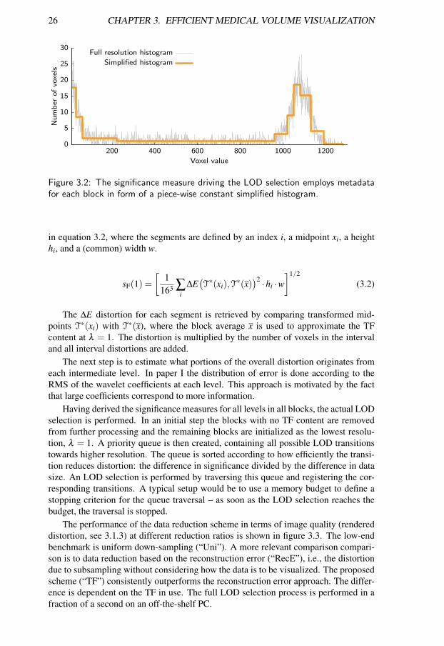
26 CHAPTER 3. EFFICIENT MEDICAL VOLUME VISUALIZATION
0
5
10
15
20
25
30
200 400 600 800 1000 1200
Num
ber
ofvo
xels
Voxel value
Full resolution histogram
Simplified histogram
Figure 3.2: The significance measure driving the LOD selection employs metadatafor each block in form of a piece-wise constant simplified histogram.
in equation 3.2, where the segments are defined by an index i, a midpoint xi, a heighthi, and a (common) width w.
sF(1) =[
1163 ∑
i∆E
(T∗(xi),T∗(x)
)2 ·hi ·w]1/2
(3.2)
The ∆E distortion for each segment is retrieved by comparing transformed mid-points T∗(xi) with T∗(x), where the block average x is used to approximate the TFcontent at λ = 1. The distortion is multiplied by the number of voxels in the intervaland all interval distortions are added.
The next step is to estimate what portions of the overall distortion originates fromeach intermediate level. In paper I the distribution of error is done according to theRMS of the wavelet coefficients at each level. This approach is motivated by the factthat large coefficients correspond to more information.
Having derived the significance measures for all levels in all blocks, the actual LODselection is performed. In an initial step the blocks with no TF content are removedfrom further processing and the remaining blocks are initialized as the lowest resolu-tion, λ = 1. A priority queue is then created, containing all possible LOD transitionstowards higher resolution. The queue is sorted according to how efficiently the transi-tion reduces distortion: the difference in significance divided by the difference in datasize. An LOD selection is performed by traversing this queue and registering the cor-responding transitions. A typical setup would be to use a memory budget to define astopping criterion for the queue traversal – as soon as the LOD selection reaches thebudget, the traversal is stopped.
The performance of the data reduction scheme in terms of image quality (rendereddistortion, see 3.1.3) at different reduction ratios is shown in figure 3.3. The low-endbenchmark is uniform down-sampling (“Uni”). A more relevant comparison compari-son is to data reduction based on the reconstruction error (“RecE”), i.e., the distortiondue to subsampling without considering how the data is to be visualized. The proposedscheme (“TF”) consistently outperforms the reconstruction error approach. The differ-ence is dependent on the TF in use. The full LOD selection process is performed in afraction of a second on an off-the-shelf PC.
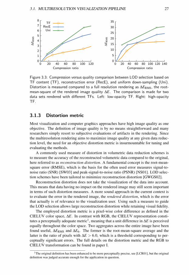
3.1. MULTIRESOLUTION VISUALIZATION PIPELINE 27
0
1
2
3
4
5
6
7
8
0 20 40 60 80 100 120
∆E
RM
S
Compression ratio
TFRecE
Uni
0
5
10
15
20
25
30
35
0 20 40 60 80 100 120 140
∆E
RM
S
Compression ratio
Figure 3.3: Compression versus quality comparison between LOD selection based onTF content (TF), reconstruction error (RecE), and uniform down-sampling (Uni).Distortion is measured compared to a full resolution rendering as ∆ERMS, the root-mean-square of the rendered image quality ∆E. The comparison is made for twodata sets rendered with different TFs. Left: low-opacity TF. Right: high-opacityTF.
3.1.3 Distortion metric
Most visualization and computer graphics approaches have high image quality as oneobjective. The definition of image quality is by no means straightforward and manyresearchers simply resort to subjective evaluations of artifacts in the rendering. Sincethe multiresolution rendering aims to maximize image quality at any given data reduc-tion level, the need for an objective distortion metric is insurmountable for tuning andevaluating the methods.
A commonly used measure of distortion in volumetric data reduction schemes isto measure the accuracy of the reconstructed volumetric data compared to the original,here referred to as reconstruction distortion. A fundamental concept is the root-mean-square error (RMSE), which is the basis for the often used error measures signal-to-noise ratio (SNR) [SW03] and peak-signal-to-noise ratio (PSNR) [NS01]. LOD selec-tion schemes have been tailored to minimize reconstruction distortion [GWGS02].
Reconstruction distortion does not take the visualization of the data into account.This means that data having no impact on the rendered image may still seem importantin terms of such distortion measures. A more sound approach in the current context isto evaluate the error in the rendered image, the rendered distortion, which is the errorthat actually is of relevance to the visualization user. Using such a measure to guidethe LOD selection allows large reconstruction distortion while retaining visual fidelity.
The employed distortion metric is a pixel-wise color difference as defined in theCIELUV color space, ∆E. In contrast with RGB, the CIELUV representation consti-tutes a perceptually adequate metric1, meaning that a unit difference in ∆E is perceivedequally throughout the color space. Two aggregates across the entire image have beenfound useful, ∆ERMS and ∆E6. The former is the root-mean-square average and thelatter is the ratio of pixels with ∆E > 6.0, which is a threshold corresponding to per-ceptually significant errors. The full details on the distortion metric and the RGB toCIELUV transformation can be found in paper I.
1The original definition has been enhanced to be more perceptually precise, see [LCR01], but the originaldefinition was judged accurate enough for the application in question.
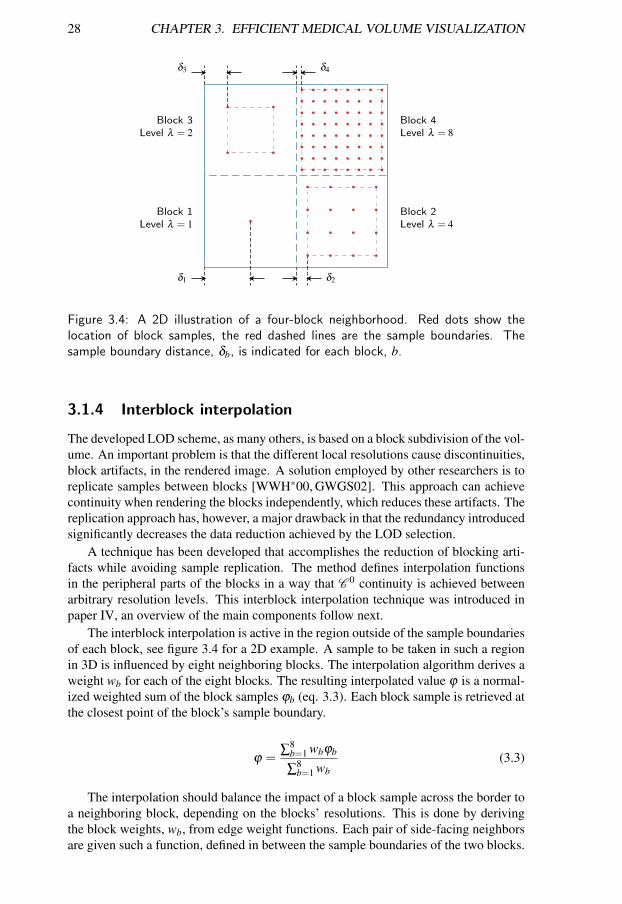
28 CHAPTER 3. EFFICIENT MEDICAL VOLUME VISUALIZATION
Block 1Level λ = 1
Block 2Level λ = 4
Block 3Level λ = 2
Block 4Level λ = 8
δ1 δ2
δ3 δ4
Figure 3.4: A 2D illustration of a four-block neighborhood. Red dots show thelocation of block samples, the red dashed lines are the sample boundaries. Thesample boundary distance, δb, is indicated for each block, b.
3.1.4 Interblock interpolation
The developed LOD scheme, as many others, is based on a block subdivision of the vol-ume. An important problem is that the different local resolutions cause discontinuities,block artifacts, in the rendered image. A solution employed by other researchers is toreplicate samples between blocks [WWH∗00, GWGS02]. This approach can achievecontinuity when rendering the blocks independently, which reduces these artifacts. Thereplication approach has, however, a major drawback in that the redundancy introducedsignificantly decreases the data reduction achieved by the LOD selection.
A technique has been developed that accomplishes the reduction of blocking arti-facts while avoiding sample replication. The method defines interpolation functionsin the peripheral parts of the blocks in a way that C 0 continuity is achieved betweenarbitrary resolution levels. This interblock interpolation technique was introduced inpaper IV, an overview of the main components follow next.
The interblock interpolation is active in the region outside of the sample boundariesof each block, see figure 3.4 for a 2D example. A sample to be taken in such a regionin 3D is influenced by eight neighboring blocks. The interpolation algorithm derives aweight wb for each of the eight blocks. The resulting interpolated value ϕ is a normal-ized weighted sum of the block samples ϕb (eq. 3.3). Each block sample is retrieved atthe closest point of the block’s sample boundary.
ϕ =∑
8b=1 wbϕb
∑8b=1 wb
(3.3)
The interpolation should balance the impact of a block sample across the border toa neighboring block, depending on the blocks’ resolutions. This is done by derivingthe block weights, wb, from edge weight functions. Each pair of side-facing neighborsare given such a function, defined in between the sample boundaries of the two blocks.
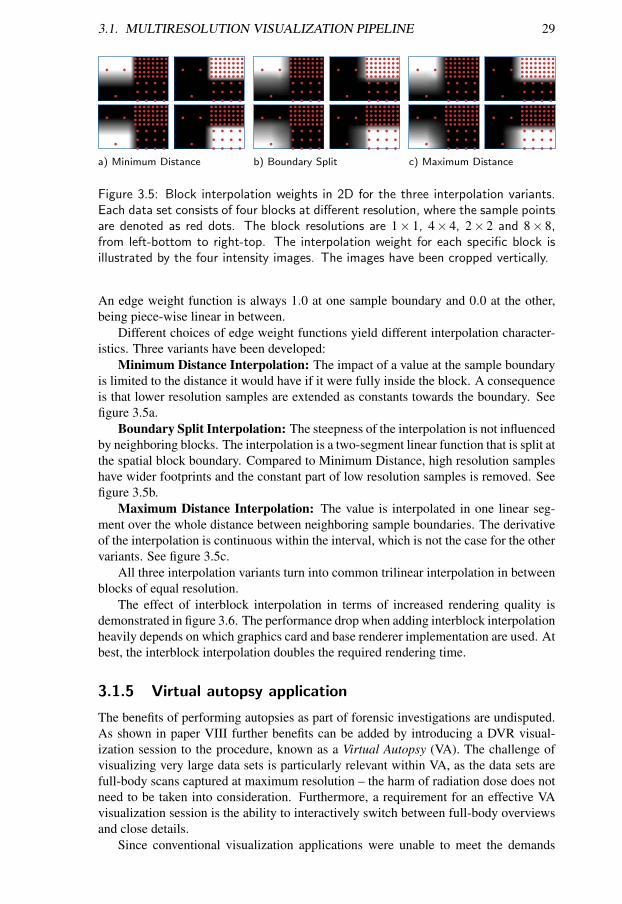
3.1. MULTIRESOLUTION VISUALIZATION PIPELINE 29
a) Minimum Distance b) Boundary Split c) Maximum Distance
Figure 3.5: Block interpolation weights in 2D for the three interpolation variants.Each data set consists of four blocks at different resolution, where the sample pointsare denoted as red dots. The block resolutions are 1× 1, 4× 4, 2× 2 and 8× 8,from left-bottom to right-top. The interpolation weight for each specific block isillustrated by the four intensity images. The images have been cropped vertically.
An edge weight function is always 1.0 at one sample boundary and 0.0 at the other,being piece-wise linear in between.
Different choices of edge weight functions yield different interpolation character-istics. Three variants have been developed:
Minimum Distance Interpolation: The impact of a value at the sample boundaryis limited to the distance it would have if it were fully inside the block. A consequenceis that lower resolution samples are extended as constants towards the boundary. Seefigure 3.5a.
Boundary Split Interpolation: The steepness of the interpolation is not influencedby neighboring blocks. The interpolation is a two-segment linear function that is split atthe spatial block boundary. Compared to Minimum Distance, high resolution sampleshave wider footprints and the constant part of low resolution samples is removed. Seefigure 3.5b.
Maximum Distance Interpolation: The value is interpolated in one linear seg-ment over the whole distance between neighboring sample boundaries. The derivativeof the interpolation is continuous within the interval, which is not the case for the othervariants. See figure 3.5c.
All three interpolation variants turn into common trilinear interpolation in betweenblocks of equal resolution.
The effect of interblock interpolation in terms of increased rendering quality isdemonstrated in figure 3.6. The performance drop when adding interblock interpolationheavily depends on which graphics card and base renderer implementation are used. Atbest, the interblock interpolation doubles the required rendering time.
3.1.5 Virtual autopsy application
The benefits of performing autopsies as part of forensic investigations are undisputed.As shown in paper VIII further benefits can be added by introducing a DVR visual-ization session to the procedure, known as a Virtual Autopsy (VA). The challenge ofvisualizing very large data sets is particularly relevant within VA, as the data sets arefull-body scans captured at maximum resolution – the harm of radiation dose does notneed to be taken into consideration. Furthermore, a requirement for an effective VAvisualization session is the ability to interactively switch between full-body overviewsand close details.
Since conventional visualization applications were unable to meet the demands
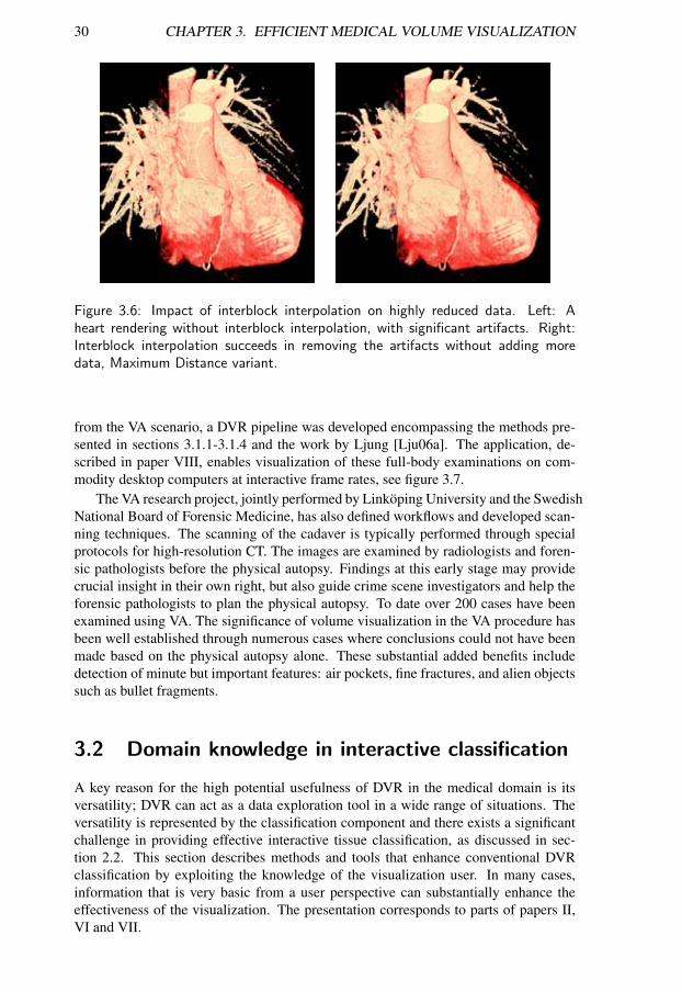
30 CHAPTER 3. EFFICIENT MEDICAL VOLUME VISUALIZATION
Figure 3.6: Impact of interblock interpolation on highly reduced data. Left: Aheart rendering without interblock interpolation, with significant artifacts. Right:Interblock interpolation succeeds in removing the artifacts without adding moredata, Maximum Distance variant.
from the VA scenario, a DVR pipeline was developed encompassing the methods pre-sented in sections 3.1.1-3.1.4 and the work by Ljung [Lju06a]. The application, de-scribed in paper VIII, enables visualization of these full-body examinations on com-modity desktop computers at interactive frame rates, see figure 3.7.
The VA research project, jointly performed by Linkoping University and the SwedishNational Board of Forensic Medicine, has also defined workflows and developed scan-ning techniques. The scanning of the cadaver is typically performed through specialprotocols for high-resolution CT. The images are examined by radiologists and foren-sic pathologists before the physical autopsy. Findings at this early stage may providecrucial insight in their own right, but also guide crime scene investigators and help theforensic pathologists to plan the physical autopsy. To date over 200 cases have beenexamined using VA. The significance of volume visualization in the VA procedure hasbeen well established through numerous cases where conclusions could not have beenmade based on the physical autopsy alone. These substantial added benefits includedetection of minute but important features: air pockets, fine fractures, and alien objectssuch as bullet fragments.
3.2 Domain knowledge in interactive classification
A key reason for the high potential usefulness of DVR in the medical domain is itsversatility; DVR can act as a data exploration tool in a wide range of situations. Theversatility is represented by the classification component and there exists a significantchallenge in providing effective interactive tissue classification, as discussed in sec-tion 2.2. This section describes methods and tools that enhance conventional DVRclassification by exploiting the knowledge of the visualization user. In many cases,information that is very basic from a user perspective can substantially enhance theeffectiveness of the visualization. The presentation corresponds to parts of papers II,VI and VII.
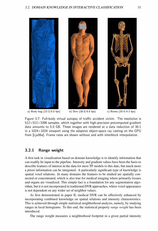
3.2. DOMAIN KNOWLEDGE IN INTERACTIVE CLASSIFICATION 31
a) Body bag (23.3/5.0 fps) b) Skin (38.0/8.8 fps) c) Bones (20.4/4.3 fps)
Figure 3.7: Full-body virtual autopsy of traffic accident victim. The resolution is512×512×3396 samples, which together with high-precision precomputed gradientdata amounts to 5.0 GB. These images are rendered at a data reduction of 30:1in a 1024×1024 viewport using the adaptive object-space ray casting on the GPUfrom [Lju06a]. Frame rates are shown without and with interblock interpolation.
3.2.1 Range weight
A first task in visualization based on domain knowledge is to identify information thatcan readily be input to the pipeline. Intensity and gradient values have been the basis todescribe features of interest in the data for most TF models to this date, but much morea priori information can be integrated. A particularly significant type of knowledge isspatial voxel relations. In many domains the features to be studied are spatially con-nected or concentrated, which is also true for medical imaging where primarily tissuesand organs are visualized. This simple fact is a foundation for any segmentation algo-rithm, but it is not incorporated in traditional DVR approaches, where voxel appearanceis not dependent on any wider set of neighbor values.
As first demonstrated in paper II, medical DVR can be effectively enhanced byincorporating combined knowledge on spatial relations and intensity characteristics.This is achieved through simple statistical neighborhood analysis, namely, by studyingranges in local histograms. To this end, the statistical property range weight has beenintroduced.
The range weight measures a neighborhood footprint in a given partial intensity
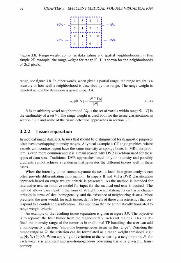
32 CHAPTER 3. EFFICIENT MEDICAL VOLUME VISUALIZATION
1
0
2
1
2
1
1
3
0
3
2
2
1
0
2
3
75%
50%
75%
0%
Figure 3.8: Range weight combines data values and spatial neighborhoods. In thissimple 2D example, the range weight for range [0..1] is shown for the neighborhoodsof 2x2 pixels.
range, see figure 3.8. In other words, when given a partial range, the range weight is ameasure of how well a neighborhood is described by that range. The range weight isdenoted wr and the definition is given in eq. 3.4.
wr(Φ,N) =|N∩VΦ||N|
(3.4)
N is an arbitrary voxel neighborhood, VΦ is the set of voxels within range Φ. |V | isthe cardinality of a set V . The range weight is used both for the tissue classification insection 3.2.2 and some of the tissue detection approaches in section 3.3.
3.2.2 Tissue separation
In medical image data sets, tissues that should be distinguished for diagnostic purposesoften have overlapping intensity ranges. A typical example is CT angiographies, wherevessels with contrast agent have the same intensity as spongy bone. In MRI, the prob-lem is even more common and it is a main reason why DVR is seldom used for thesetypes of data sets. Traditional DVR approaches based only on intensity and possiblygradients cannot achieve a rendering that separates the different tissues well in thesecases.
When the intensity alone cannot separate tissues, a local histogram analysis canoften provide differentiating information. In papers II and VII a DVR classificationapproach based on range weight criteria is presented. As the method is intended forinteractive use, an intuitive model for input for the medical end-user is desired. Themethod allows user input in the form of straightforward statements on tissue charac-teristics in terms of size, homogeneity, and the existence of neighboring tissues. Moreprecisely, the user would, for each tissue, define levels of these characteristics that cor-respond to a confident classification. This input can then be automatically translated torange weight criteria.
An example of the resulting tissue separation is given in figure 3.9. The objectiveis to separate the liver tumor from the diagnostically irrelevant regions. Having de-fined the intensity range of the tumor as in traditional TF handling, the user can adda homogeneity criterion: “show me homogeneous tissue in this range”. Denoting thetumor range as Φ, the criterion can be formulated as a range weight threshold, e.g.:wr(Φ,Nv)≥ 0.6. When applying this criterion to the rendering, a neighborhood Nv foreach voxel v is analyzed and non-homogeneous obscuring tissue is given full trans-parency.
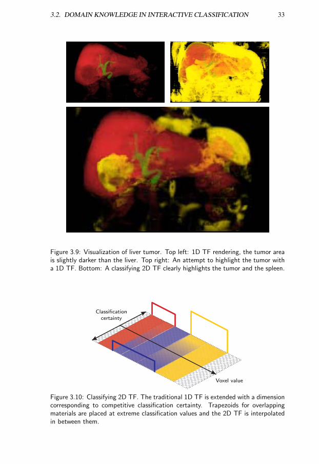
3.2. DOMAIN KNOWLEDGE IN INTERACTIVE CLASSIFICATION 33
Figure 3.9: Visualization of liver tumor. Top left: 1D TF rendering, the tumor areais slightly darker than the liver. Top right: An attempt to highlight the tumor witha 1D TF. Bottom: A classifying 2D TF clearly highlights the tumor and the spleen.
Classificationcertainty
Voxel value
Figure 3.10: Classifying 2D TF. The traditional 1D TF is extended with a dimensioncorresponding to competitive classification certainty. Trapezoids for overlappingmaterials are placed at extreme classification values and the 2D TF is interpolatedin between them.
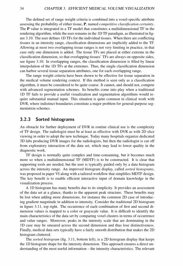
34 CHAPTER 3. EFFICIENT MEDICAL VOLUME VISUALIZATION
The defined set of range weight criteria is combined into a voxel-specific attributeassessing the probability of either tissue, P, named competitive classification certainty.The P value is integrated in a TF model that constitutes a multidimensional TF in therendering algorithm, while the user remains in the 1D TF paradigm, as illustrated in fig-ure 3.10. The user defines 1D TFs for the individual tissues. When there are conflictingtissues in an intensity range, classification dimensions are implicitly added to the TF.Allowing at most two overlapping tissue ranges is not very limiting in practice, in thatcase only one dimension is added. The tissue TFs are placed at either extreme in theclassification dimension, so that overlapping tissues’ TFs are always on opposite sides,see figure 3.10. In overlapping ranges, the classification dimension is filled by linearinterpolation of the 1D TFs at the extremes. Thus, the single classification dimensioncan harbor several tissue separation attributes, one for each overlapping range.
The range weight criteria have been shown to be effective for tissue separation inthe medical volume rendering context. If this method is seen only as a classificationalgorithm, it must be considered to be quite coarse. It cannot, and should not, competewith advanced segmentation schemes. Its benefits come into play when a traditional1D TF fails to provide a useful visualization and segmentation algorithms would re-quire substantial manual input. This situation is quite common in clinical work withDVR, where indistinct boundaries constitute a major problem for general-purpose seg-mentation schemes.
3.2.3 Sorted histograms
An obstacle for further deployment of DVR in routine clinical use is the complexityof TF design. The radiologist must be at least as effective with DVR as with 2D sliceviewing in order to adopt the new technique. Today many hospitals organize dedicated3D labs producing DVR images for the radiologists, but then the radiologist is cut offfrom exploratory interaction of the data set, which may lead to lower quality in thediagnostic work.
TF design is normally quite complex and time-consuming, but it becomes muchmore so when a multidimensional TF (MDTF) is to be constructed. It is clear thatsupporting tools are needed, but the user is typically guided only by a data histogramacross the intensity range. An improved histogram display, called sorted histograms,was proposed in paper VI along with a tailored workflow that simplifies MDTF design.The key benefit is to enable efficient interactive input of domain knowledge in thevisualization process.
A 1D histogram has many benefits due to its simplicity. It provides an assessmentof the data set at a glance, thanks to the apparent peak structure. These benefits maybe lost when adding more dimensions, for instance the common 2D case of introduc-ing gradient magnitude in addition to intensity. Consider the traditional 2D histogramin figure 3.11, top right. The occurrence of each combination of first and second di-mension values is mapped to a color or grayscale value. It is difficult to identify themain characteristics of the data set by comparing voxel clusters in terms of occurrenceand value ranges. Moreover, peaks in the intensity scale that are dominating in the1D case may be smeared across the second dimension and thus lose distinctiveness.Finally, medical data sets typically have a fairly smooth distribution that makes the 2Dhistogram cluttered.
The sorted histogram (fig. 3.11, bottom left), is a 2D histogram display that keepsthe 1D histogram shape for the intensity dimension. This approach ensures a direct un-derstanding of the most useful information – the intensity characteristics. The relevant
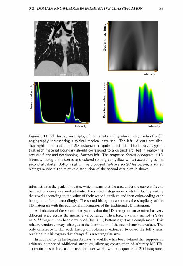
3.2. DOMAIN KNOWLEDGE IN INTERACTIVE CLASSIFICATION 35
Gra
die
nt
magnitude
Intensity
Num
ber
ofvo
xels
Intensity
Rel
ative
num
ber
ofvo
xels
Intensity
Figure 3.11: 2D histogram displays for intensity and gradient magnitude of a CTangiography representing a typical medical data set. Top left: A data set slice.Top right: The traditional 2D histogram is quite indistinct. The theory suggeststhat each material boundary should correspond to a distinct arc, but in reality thearcs are fuzzy and overlapping. Bottom left: The proposed Sorted histogram, a 1Dintensity histogram is sorted and colored (blue-green-yellow-white) according to thesecond attribute. Bottom right: The proposed Relative sorted histogram, a sortedhistogram where the relative distribution of the second attribute is shown.
information is the peak silhouette, which means that the area under the curve is free tobe used to convey a second attribute. The sorted histogram exploits this fact by sortingthe voxels according to the value of their second attribute and then color-coding eachhistogram column accordingly. The sorted histogram combines the simplicity of the1D histogram with the additional information of the traditional 2D histogram.
A limitation of the sorted histogram is that the 1D histogram curve often has verydifferent scale across the intensity value range. Therefore, a variant named relativesorted histogram has been developed (fig. 3.11, bottom right) as a complement. Thisrelative version conveys changes in the distribution of the second attribute values. Theonly difference is that each histogram column is extended to cover the full y-axis,resulting in a histogram that always fills a rectangular area.
In addition to the histogram displays, a workflow has been defined that supports anarbitrary number of additional attributes, allowing construction of arbitrary MDTFs.To retain reasonable ease-of-use, the user works with a sequence of 2D histograms,
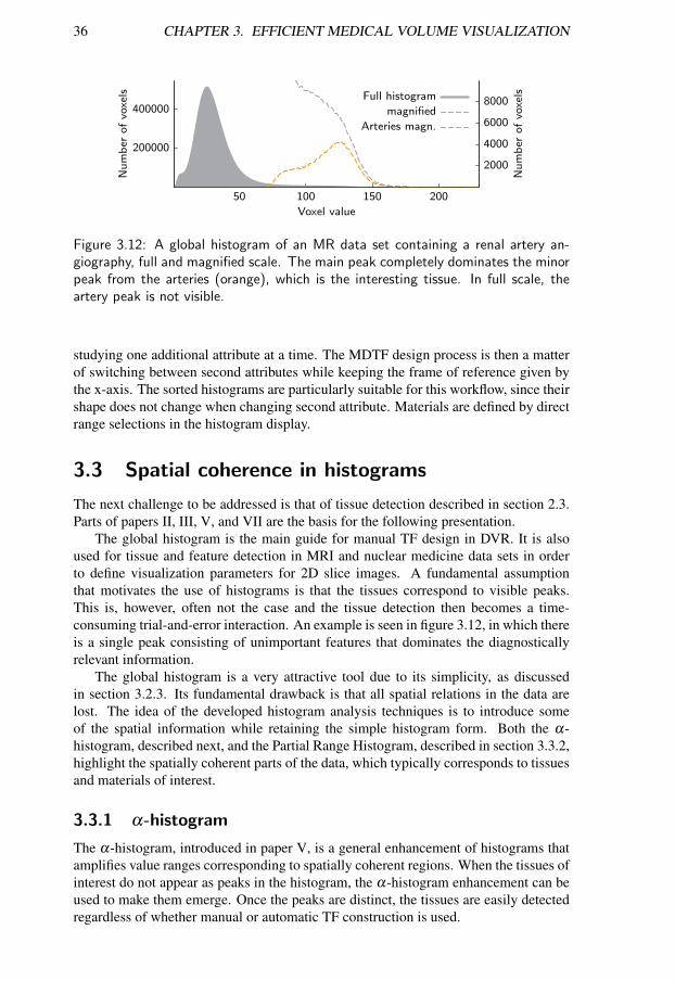
36 CHAPTER 3. EFFICIENT MEDICAL VOLUME VISUALIZATION
400000
200000
50 100 150 200
8000
6000
4000
2000
Num
ber
ofvo
xels
Num
ber
ofvo
xels
Voxel value
Full histogram
magnified
Arteries magn.
Figure 3.12: A global histogram of an MR data set containing a renal artery an-giography, full and magnified scale. The main peak completely dominates the minorpeak from the arteries (orange), which is the interesting tissue. In full scale, theartery peak is not visible.
studying one additional attribute at a time. The MDTF design process is then a matterof switching between second attributes while keeping the frame of reference given bythe x-axis. The sorted histograms are particularly suitable for this workflow, since theirshape does not change when changing second attribute. Materials are defined by directrange selections in the histogram display.
3.3 Spatial coherence in histograms
The next challenge to be addressed is that of tissue detection described in section 2.3.Parts of papers II, III, V, and VII are the basis for the following presentation.
The global histogram is the main guide for manual TF design in DVR. It is alsoused for tissue and feature detection in MRI and nuclear medicine data sets in orderto define visualization parameters for 2D slice images. A fundamental assumptionthat motivates the use of histograms is that the tissues correspond to visible peaks.This is, however, often not the case and the tissue detection then becomes a time-consuming trial-and-error interaction. An example is seen in figure 3.12, in which thereis a single peak consisting of unimportant features that dominates the diagnosticallyrelevant information.
The global histogram is a very attractive tool due to its simplicity, as discussedin section 3.2.3. Its fundamental drawback is that all spatial relations in the data arelost. The idea of the developed histogram analysis techniques is to introduce someof the spatial information while retaining the simple histogram form. Both the α-histogram, described next, and the Partial Range Histogram, described in section 3.3.2,highlight the spatially coherent parts of the data, which typically corresponds to tissuesand materials of interest.
3.3.1 α-histogram
The α-histogram, introduced in paper V, is a general enhancement of histograms thatamplifies value ranges corresponding to spatially coherent regions. When the tissues ofinterest do not appear as peaks in the histogram, the α-histogram enhancement can beused to make them emerge. Once the peaks are distinct, the tissues are easily detectedregardless of whether manual or automatic TF construction is used.
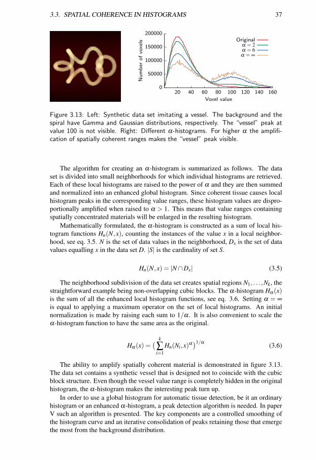
3.3. SPATIAL COHERENCE IN HISTOGRAMS 37
0
50000
100000
150000
200000
20 40 60 80 100 120 140 160
Num
ber
ofvo
xels
Voxel value
Originalα = 2α = 6α = ∞
Figure 3.13: Left: Synthetic data set imitating a vessel. The background and thespiral have Gamma and Gaussian distributions, respectively. The “vessel” peak atvalue 100 is not visible. Right: Different α-histograms. For higher α the amplifi-cation of spatially coherent ranges makes the “vessel” peak visible.
The algorithm for creating an α-histogram is summarized as follows. The dataset is divided into small neighborhoods for which individual histograms are retrieved.Each of these local histograms are raised to the power of α and they are then summedand normalized into an enhanced global histogram. Since coherent tissue causes localhistogram peaks in the corresponding value ranges, these histogram values are dispro-portionally amplified when raised to α > 1. This means that value ranges containingspatially concentrated materials will be enlarged in the resulting histogram.
Mathematically formulated, the α-histogram is constructed as a sum of local his-togram functions Hn(N,x), counting the instances of the value x in a local neighbor-hood, see eq. 3.5. N is the set of data values in the neighborhood, Dx is the set of datavalues equalling x in the data set D. |S| is the cardinality of set S.
Hn(N,x) = |N∩Dx| (3.5)
The neighborhood subdivision of the data set creates spatial regions N1, . . . ,Nk, thestraightforward example being non-overlapping cubic blocks. The α-histogram Hα(x)is the sum of all the enhanced local histogram functions, see eq. 3.6. Setting α = ∞
is equal to applying a maximum operator on the set of local histograms. An initialnormalization is made by raising each sum to 1/α . It is also convenient to scale theα-histogram function to have the same area as the original.
Hα(x) =( k
∑i=1
Hn(Ni,x)α)1/α (3.6)
The ability to amplify spatially coherent material is demonstrated in figure 3.13.The data set contains a synthetic vessel that is designed not to coincide with the cubicblock structure. Even though the vessel value range is completely hidden in the originalhistogram, the α-histogram makes the interesting peak turn up.
In order to use a global histogram for automatic tissue detection, be it an ordinaryhistogram or an enhanced α-histogram, a peak detection algorithm is needed. In paperV such an algorithm is presented. The key components are a controlled smoothing ofthe histogram curve and an iterative consolidation of peaks retaining those that emergethe most from the background distribution.
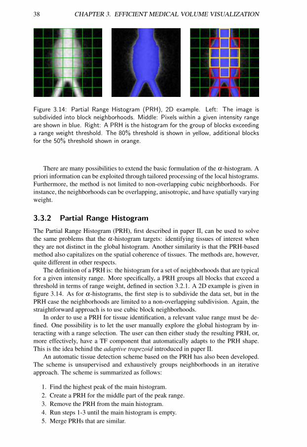
38 CHAPTER 3. EFFICIENT MEDICAL VOLUME VISUALIZATION
Figure 3.14: Partial Range Histogram (PRH), 2D example. Left: The image issubdivided into block neighborhoods. Middle: Pixels within a given intensity rangeare shown in blue. Right: A PRH is the histogram for the group of blocks exceedinga range weight threshold. The 80% threshold is shown in yellow, additional blocksfor the 50% threshold shown in orange.
There are many possibilities to extend the basic formulation of the α-histogram. Apriori information can be exploited through tailored processing of the local histograms.Furthermore, the method is not limited to non-overlapping cubic neighborhoods. Forinstance, the neighborhoods can be overlapping, anisotropic, and have spatially varyingweight.
3.3.2 Partial Range Histogram
The Partial Range Histogram (PRH), first described in paper II, can be used to solvethe same problems that the α-histogram targets: identifying tissues of interest whenthey are not distinct in the global histogram. Another similarity is that the PRH-basedmethod also capitalizes on the spatial coherence of tissues. The methods are, however,quite different in other respects.
The definition of a PRH is: the histogram for a set of neighborhoods that are typicalfor a given intensity range. More specifically, a PRH groups all blocks that exceed athreshold in terms of range weight, defined in section 3.2.1. A 2D example is given infigure 3.14. As for α-histograms, the first step is to subdivide the data set, but in thePRH case the neighborhoods are limited to a non-overlapping subdivision. Again, thestraightforward approach is to use cubic block neighborhoods.
In order to use a PRH for tissue identification, a relevant value range must be de-fined. One possibility is to let the user manually explore the global histogram by in-teracting with a range selection. The user can then either study the resulting PRH, or,more effectively, have a TF component that automatically adapts to the PRH shape.This is the idea behind the adaptive trapezoid introduced in paper II.
An automatic tissue detection scheme based on the PRH has also been developed.The scheme is unsupervised and exhaustively groups neighborhoods in an iterativeapproach. The scheme is summarized as follows:
1. Find the highest peak of the main histogram.2. Create a PRH for the middle part of the peak range.3. Remove the PRH from the main histogram.4. Run steps 1-3 until the main histogram is empty.5. Merge PRHs that are similar.
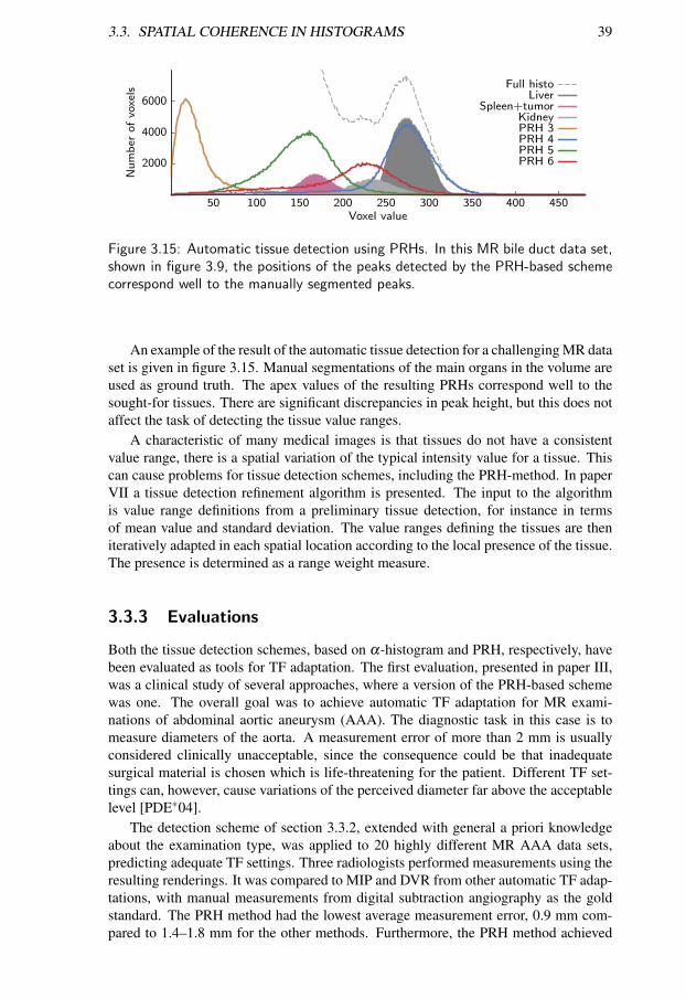
3.3. SPATIAL COHERENCE IN HISTOGRAMS 39
6000
4000
2000
50 100 150 200 250 300 350 400 450
Num
ber
ofvo
xels
Voxel value
Full histoLiver
Spleen+tumorKidneyPRH 3PRH 4PRH 5PRH 6
Figure 3.15: Automatic tissue detection using PRHs. In this MR bile duct data set,shown in figure 3.9, the positions of the peaks detected by the PRH-based schemecorrespond well to the manually segmented peaks.
An example of the result of the automatic tissue detection for a challenging MR dataset is given in figure 3.15. Manual segmentations of the main organs in the volume areused as ground truth. The apex values of the resulting PRHs correspond well to thesought-for tissues. There are significant discrepancies in peak height, but this does notaffect the task of detecting the tissue value ranges.
A characteristic of many medical images is that tissues do not have a consistentvalue range, there is a spatial variation of the typical intensity value for a tissue. Thiscan cause problems for tissue detection schemes, including the PRH-method. In paperVII a tissue detection refinement algorithm is presented. The input to the algorithmis value range definitions from a preliminary tissue detection, for instance in termsof mean value and standard deviation. The value ranges defining the tissues are theniteratively adapted in each spatial location according to the local presence of the tissue.The presence is determined as a range weight measure.
3.3.3 Evaluations
Both the tissue detection schemes, based on α-histogram and PRH, respectively, havebeen evaluated as tools for TF adaptation. The first evaluation, presented in paper III,was a clinical study of several approaches, where a version of the PRH-based schemewas one. The overall goal was to achieve automatic TF adaptation for MR exami-nations of abdominal aortic aneurysm (AAA). The diagnostic task in this case is tomeasure diameters of the aorta. A measurement error of more than 2 mm is usuallyconsidered clinically unacceptable, since the consequence could be that inadequatesurgical material is chosen which is life-threatening for the patient. Different TF set-tings can, however, cause variations of the perceived diameter far above the acceptablelevel [PDE∗04].
The detection scheme of section 3.3.2, extended with general a priori knowledgeabout the examination type, was applied to 20 highly different MR AAA data sets,predicting adequate TF settings. Three radiologists performed measurements using theresulting renderings. It was compared to MIP and DVR from other automatic TF adap-tations, with manual measurements from digital subtraction angiography as the goldstandard. The PRH method had the lowest average measurement error, 0.9 mm com-pared to 1.4–1.8 mm for the other methods. Furthermore, the PRH method achieved
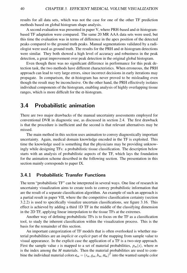
40 CHAPTER 3. EFFICIENT MEDICAL VOLUME VISUALIZATION
results for all data sets, which was not the case for one of the other TF predictionmethods based on global histogram shape analysis.
A second evaluation was presented in paper V, where PRH-based and α-histogram-based TF adaptation were compared. The same 20 MR AAA data sets were used, butthis time the evaluation was in terms of difference in the apex position of the detectedpeaks compared to the ground truth peaks. Manual segmentations validated by a radi-ologist were used as ground truth. The results for the PRH and α-histogram detectionswere similar. They both showed a high level of accuracy and robustness in the peakdetection, a great improvement over peak detection in the original global histogram.
Even though there was no significant difference in performance for this peak de-tection task, the two methods have different characteristics. When erroneous, the PRHapproach can lead to very large errors, since incorrect decisions in early iterations maypropagate. In comparison, the α-histogram has never proved to be misleading eventhough the result may be inconclusive. On the other hand, the PRH effectively isolatesindividual components of the histogram, enabling analysis of highly overlapping tissueranges, which is more difficult for the α-histogram.
3.4 Probabilistic animation
There are two major drawbacks of the manual uncertainty assessments employed forconventional DVR in diagnostic use, as discussed in section 2.4. The first drawbackis that the procedure is inefficient and the second is that relevant alternatives may bemissed.
The main method in this section uses animation to convey diagnostically importantuncertainty. Again, medical domain knowledge encoded in the TF is exploited. Thistime the knowledge used is something that the physicians may be providing unknow-ingly while designing TFs: a probabilistic tissue classification. The description belowstarts with an analysis of probabilistic aspects of the TF, which lays the foundationfor the animation scheme described in the following section. The presentation in thissection mainly corresponds to paper IX.
3.4.1 Probabilistic Transfer Functions
The term “probabilistic TF” can be interpreted in several ways. One line of research inuncertainty visualization aims to create tools to convey probabilistic information thatare the result of a separate classification algorithm. An example of such an approach isa partial result in paper VII, where the the competitive classification certainty (section3.2.2) is used to specifically visualize uncertain classifications, see figure 3.16. Thiseffect is achieved by adding a third 1D TF in the middle of the classifying dimensionin the 2D TF, applying linear interpolation to the tissue TFs at the extremes.
Another way of defining probabilistic TFs is to focus on the TF as a classificationtool, to study the inherent classification within the visualization process. This is thebasis for the remainder of this section.
An important categorization of TF models that is often overlooked is whether ma-terial probabilities are an implicit or explicit part of the mapping from sample value tovisual appearance. In the explicit case the application of a TF is a two-step approach.First the sample value s is mapped to a set of material probabilities, pm(s), where mis the index among the M materials. Then the material probabilities are used to com-bine the individual material colors cm = (rm,gm,bm,αm)T into the wanted sample color
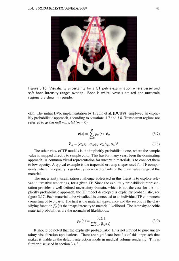
3.4. PROBABILISTIC ANIMATION 41
Figure 3.16: Visualizing uncertainty for a CT pelvis examination where vessel andsoft bone intensity ranges overlap. Bone is white, vessels are red and uncertainregions are shown in purple.
c(s). The initial DVR implementation by Drebin et al. [DCH88] employed an explic-itly probabilistic approach, according to equations 3.7 and 3.8. Transparent regions arereferred to as the null material (m = 0).
c(s) =M
∑m=0
pm(s) · cm (3.7)
cm = (αmrm, αmgm, αmbm, αm)T (3.8)
The other view of TF models is the implicitly probabilistic one, where the samplevalue is mapped directly to sample color. This has for many years been the dominatingapproach. A common visual representation for uncertain materials is to connect themto low opacity. A typical example is the trapezoid or ramp shapes used for TF compo-nents, where the opacity is gradually decreased outside of the main value range of thematerial.
The uncertainty visualization challenge addressed in this thesis is to explore rele-vant alternative renderings, for a given TF. Since the explicitly probabilistic represen-tation provides a well-defined uncertainty domain, which is not the case for the im-plicitly probabilistic approach, the TF model developed is explicitly probabilistic, seefigure 3.17. Each material to be visualized is connected to an individual TF componentconsisting of two parts. The first is the material appearance and the second is the clas-sifying function pm(s) that maps intensity to material likelihood. The intensity-specificmaterial probabilities are the normalized likelihoods:
pm(s) =pm(s)
∑Mm′=0 pm′(s)
(3.9)
It should be noted that the explicitly probabilistic TF is not limited to pure uncer-tainty visualization applications. There are significant benefits of this approach thatmakes it viable as the default interaction mode in medical volume rendering. This isfurther discussed in section 3.4.3.
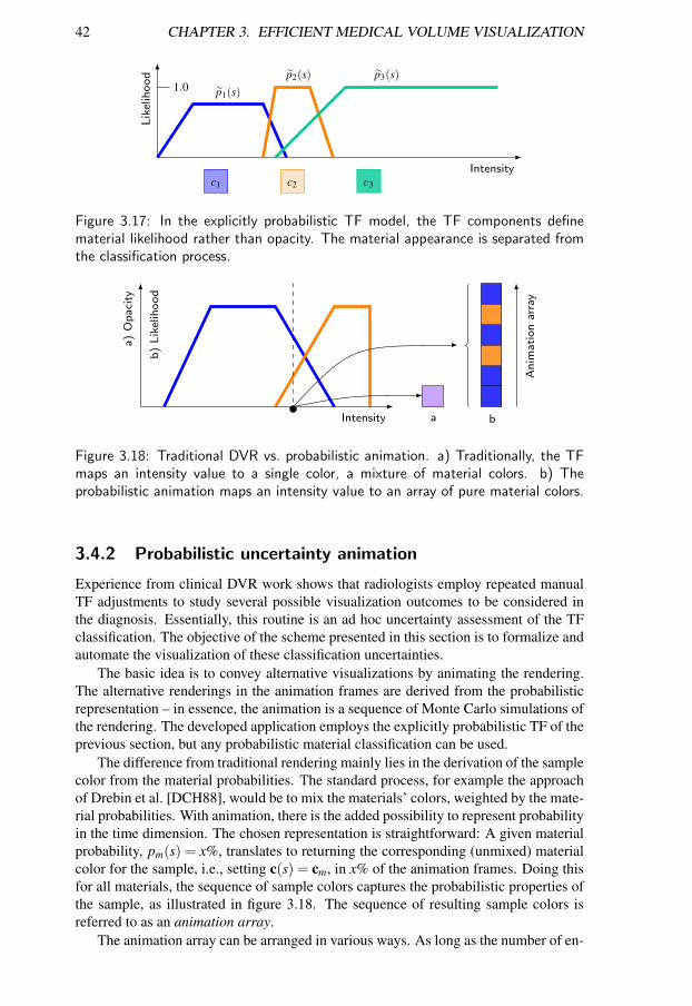
42 CHAPTER 3. EFFICIENT MEDICAL VOLUME VISUALIZATION
Lik
elih
ood
1.0
Intensityc1 c2 c3
p1(s)p2(s) p3(s)
Figure 3.17: In the explicitly probabilistic TF model, the TF components definematerial likelihood rather than opacity. The material appearance is separated fromthe classification process.
a)
Opaci
ty
b)
Lik
elih
ood
Intensity a b
Anim
ation
arra
y
Figure 3.18: Traditional DVR vs. probabilistic animation. a) Traditionally, the TFmaps an intensity value to a single color, a mixture of material colors. b) Theprobabilistic animation maps an intensity value to an array of pure material colors.
3.4.2 Probabilistic uncertainty animation
Experience from clinical DVR work shows that radiologists employ repeated manualTF adjustments to study several possible visualization outcomes to be considered inthe diagnosis. Essentially, this routine is an ad hoc uncertainty assessment of the TFclassification. The objective of the scheme presented in this section is to formalize andautomate the visualization of these classification uncertainties.
The basic idea is to convey alternative visualizations by animating the rendering.The alternative renderings in the animation frames are derived from the probabilisticrepresentation – in essence, the animation is a sequence of Monte Carlo simulations ofthe rendering. The developed application employs the explicitly probabilistic TF of theprevious section, but any probabilistic material classification can be used.
The difference from traditional rendering mainly lies in the derivation of the samplecolor from the material probabilities. The standard process, for example the approachof Drebin et al. [DCH88], would be to mix the materials’ colors, weighted by the mate-rial probabilities. With animation, there is the added possibility to represent probabilityin the time dimension. The chosen representation is straightforward: A given materialprobability, pm(s) = x%, translates to returning the corresponding (unmixed) materialcolor for the sample, i.e., setting c(s) = cm, in x% of the animation frames. Doing thisfor all materials, the sequence of sample colors captures the probabilistic properties ofthe sample, as illustrated in figure 3.18. The sequence of resulting sample colors isreferred to as an animation array.
The animation array can be arranged in various ways. As long as the number of en-
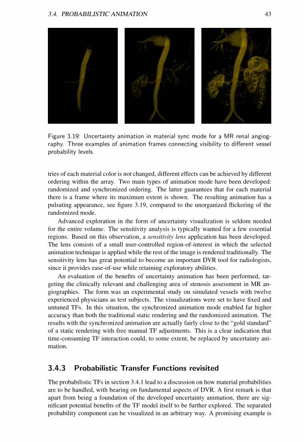
3.4. PROBABILISTIC ANIMATION 43
Figure 3.19: Uncertainty animation in material sync mode for a MR renal angiog-raphy. Three examples of animation frames connecting visibility to different vesselprobability levels.
tries of each material color is not changed, different effects can be achieved by differentordering within the array. Two main types of animation mode have been developed:randomized and synchronized ordering. The latter guarantees that for each materialthere is a frame where its maximum extent is shown. The resulting animation has apulsating appearance, see figure 3.19, compared to the unorganized flickering of therandomized mode.
Advanced exploration in the form of uncertainty visualization is seldom neededfor the entire volume. The sensitivity analysis is typically wanted for a few essentialregions. Based on this observation, a sensitivity lens application has been developed.The lens consists of a small user-controlled region-of-interest in which the selectedanimation technique is applied while the rest of the image is rendered traditionally. Thesensitivity lens has great potential to become an important DVR tool for radiologists,since it provides ease-of-use while retaining exploratory abilities.
An evaluation of the benefits of uncertainty animation has been performed, tar-geting the clinically relevant and challenging area of stenosis assessment in MR an-giographies. The form was an experimental study on simulated vessels with twelveexperienced physicians as test subjects. The visualizations were set to have fixed anduntuned TFs. In this situation, the synchronized animation mode enabled far higheraccuracy than both the traditional static rendering and the randomized animation. Theresults with the synchronized animation are actually fairly close to the “gold standard”of a static rendering with free manual TF adjustments. This is a clear indication thattime-consuming TF interaction could, to some extent, be replaced by uncertainty ani-mation.
3.4.3 Probabilistic Transfer Functions revisited
The probabilistic TFs in section 3.4.1 lead to a discussion on how material probabilitiesare to be handled, with bearing on fundamental aspects of DVR. A first remark is thatapart from being a foundation of the developed uncertainty animation, there are sig-nificant potential benefits of the TF model itself to be further explored. The separatedprobability component can be visualized in an arbitrary way. A promising example is
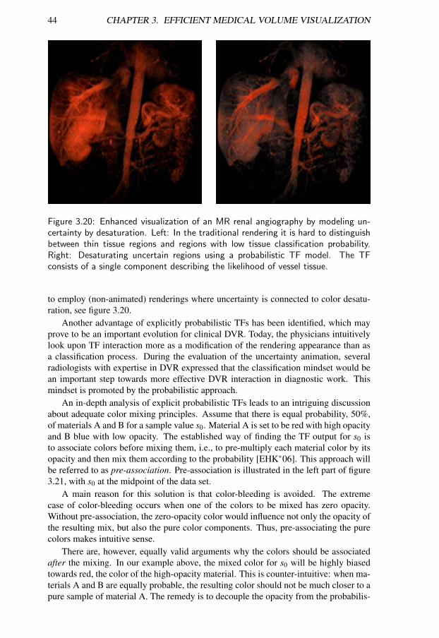
44 CHAPTER 3. EFFICIENT MEDICAL VOLUME VISUALIZATION
Figure 3.20: Enhanced visualization of an MR renal angiography by modeling un-certainty by desaturation. Left: In the traditional rendering it is hard to distinguishbetween thin tissue regions and regions with low tissue classification probability.Right: Desaturating uncertain regions using a probabilistic TF model. The TFconsists of a single component describing the likelihood of vessel tissue.
to employ (non-animated) renderings where uncertainty is connected to color desatu-ration, see figure 3.20.
Another advantage of explicitly probabilistic TFs has been identified, which mayprove to be an important evolution for clinical DVR. Today, the physicians intuitivelylook upon TF interaction more as a modification of the rendering appearance than asa classification process. During the evaluation of the uncertainty animation, severalradiologists with expertise in DVR expressed that the classification mindset would bean important step towards more effective DVR interaction in diagnostic work. Thismindset is promoted by the probabilistic approach.
An in-depth analysis of explicit probabilistic TFs leads to an intriguing discussionabout adequate color mixing principles. Assume that there is equal probability, 50%,of materials A and B for a sample value s0. Material A is set to be red with high opacityand B blue with low opacity. The established way of finding the TF output for s0 isto associate colors before mixing them, i.e., to pre-multiply each material color by itsopacity and then mix them according to the probability [EHK∗06]. This approach willbe referred to as pre-association. Pre-association is illustrated in the left part of figure3.21, with s0 at the midpoint of the data set.
A main reason for this solution is that color-bleeding is avoided. The extremecase of color-bleeding occurs when one of the colors to be mixed has zero opacity.Without pre-association, the zero-opacity color would influence not only the opacity ofthe resulting mix, but also the pure color components. Thus, pre-associating the purecolors makes intuitive sense.
There are, however, equally valid arguments why the colors should be associatedafter the mixing. In our example above, the mixed color for s0 will be highly biasedtowards red, the color of the high-opacity material. This is counter-intuitive: when ma-terials A and B are equally probable, the resulting color should not be much closer to apure sample of material A. The remedy is to decouple the opacity from the probabilis-
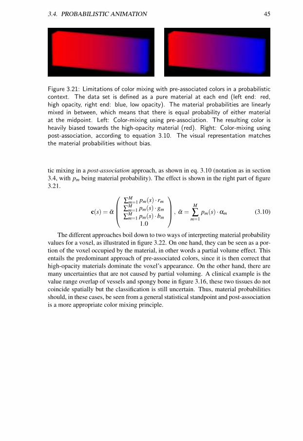
3.4. PROBABILISTIC ANIMATION 45
Figure 3.21: Limitations of color mixing with pre-associated colors in a probabilisticcontext. The data set is defined as a pure material at each end (left end: red,high opacity, right end: blue, low opacity). The material probabilities are linearlymixed in between, which means that there is equal probability of either materialat the midpoint. Left: Color-mixing using pre-association. The resulting color isheavily biased towards the high-opacity material (red). Right: Color-mixing usingpost-association, according to equation 3.10. The visual representation matchesthe material probabilities without bias.
tic mixing in a post-association approach, as shown in eq. 3.10 (notation as in section3.4, with pm being material probability). The effect is shown in the right part of figure3.21.
c(s) = α
∑
Mm=1 pm(s) · rm
∑Mm=1 pm(s) ·gm
∑Mm=1 pm(s) ·bm
1.0
, α =M
∑m=1
pm(s) ·αm (3.10)
The different approaches boil down to two ways of interpreting material probabilityvalues for a voxel, as illustrated in figure 3.22. On one hand, they can be seen as a por-tion of the voxel occupied by the material, in other words a partial volume effect. Thisentails the predominant approach of pre-associated colors, since it is then correct thathigh-opacity materials dominate the voxel’s appearance. On the other hand, there aremany uncertainties that are not caused by partial voluming. A clinical example is thevalue range overlap of vessels and spongy bone in figure 3.16, these two tissues do notcoincide spatially but the classification is still uncertain. Thus, material probabilitiesshould, in these cases, be seen from a general statistical standpoint and post-associationis a more appropriate color mixing principle.
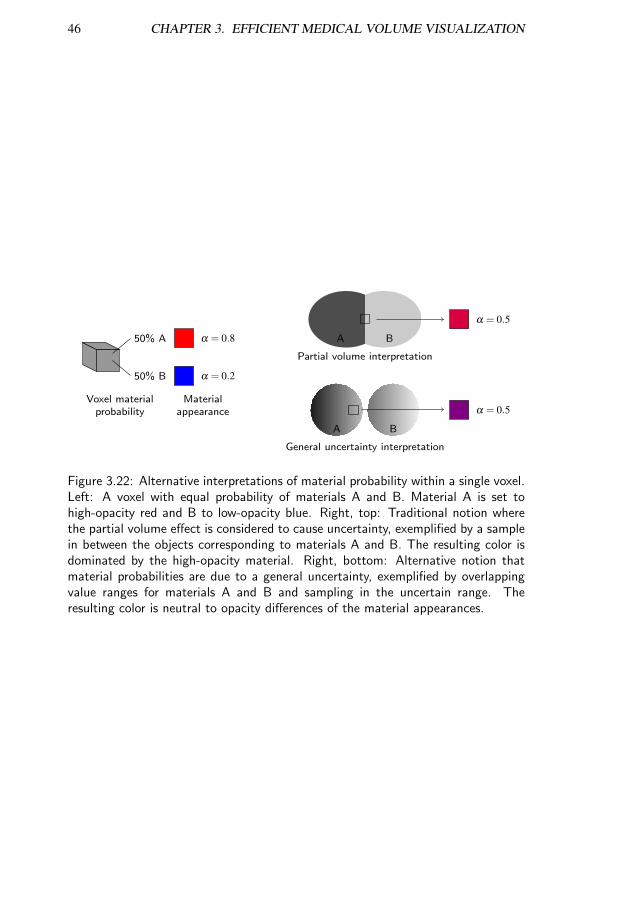
46 CHAPTER 3. EFFICIENT MEDICAL VOLUME VISUALIZATION
50% A
50% B
Voxel materialprobability
Materialappearance
α = 0.8
α = 0.2
A B
Partial volume interpretation
A B
General uncertainty interpretation
α = 0.5
α = 0.5
Figure 3.22: Alternative interpretations of material probability within a single voxel.Left: A voxel with equal probability of materials A and B. Material A is set tohigh-opacity red and B to low-opacity blue. Right, top: Traditional notion wherethe partial volume effect is considered to cause uncertainty, exemplified by a samplein between the objects corresponding to materials A and B. The resulting color isdominated by the high-opacity material. Right, bottom: Alternative notion thatmaterial probabilities are due to a general uncertainty, exemplified by overlappingvalue ranges for materials A and B and sampling in the uncertain range. Theresulting color is neutral to opacity differences of the material appearances.
Chapter 4
Conclusions
In the context of this work, visualization research can be divided into two parts. Onetrack has the objective to work with the technical methods to tune existing approachesand invent new ones. The other track is to build upon the application area of the visual-ization, to develop tools and find techniques that can make the most of the knowledgeand work context of the visualization user. Both tracks are needed for optimal progress,but the purely technical level is, today, so high that the application-centered track seemsto have the highest potential for major future advances in the field.
This thesis has described research in the application-centered track, devoted to thedevelopment of methods that contribute to the usefulness of DVR. Some concludingremarks will be made in this final chapter. First, the main research contributions of thisthesis are summarized. A mindset constituting an adequate context for the proposedmethods and future research is described next, followed by an outlook in the form oftopics for future work.
4.1 Summarized contributions
Four main obstacles for efficient medical volume visualization in a clinical contexthave been identified and addressed in this thesis:
• An effective way of handling very large data sets has been presented in the formof a multiresolution DVR pipeline with an LOD selection based on TF content.
• Enhanced capabilities and lowered complexity in interactive tissue classificationhave been achieved by incorporating basic domain knowledge in the DVR toolset.
• Improved automatic and manual tissue detection for visualization purposes hasbeen demonstrated in several schemes exploiting spatial relations in the data.
• Additional information relevant for data exploration has been achieved by auto-mated uncertainty visualization based on probabilistic TFs.
The methods have been applied in clinical visualization scenarios regarding pri-marily CT and MR data sets. DVR is commonly applied to CT examinations but israre for MR data due to the limited distinction between tissues and the noisy bound-aries. Many problems concerning visualization of CT data have been addressed. A
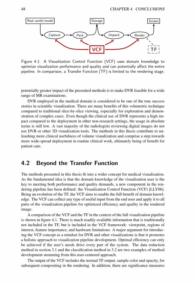
48 CHAPTER 4. CONCLUSIONS
VCF TF
Capture Pack Unpack Render
Real world/model Storage Screen
Figure 4.1: A Visualization Control Function (VCF) uses domain knowledge tooptimize visualization performance and quality and can potentially affect the entirepipeline. In comparison, a Transfer Function (TF) is limited to the rendering stage.
potentially greater impact of the presented methods is to make DVR feasible for a widerange of MR examinations.
DVR employed in the medical domain is considered to be one of the true successstories in scientific visualization. There are many benefits of this volumetric techniquecompared to traditional slice-by-slice viewing, especially for exploration and demon-stration of complex cases. Even though the clinical use of DVR represents a high im-pact compared to the deployment in other non-research settings, the usage in absoluteterms is still low. A vast majority of the radiologists reviewing digital images do notuse DVR or other 3D visualization tools. The methods in this thesis contribute to un-leashing more clinical usefulness of volume visualization and comprise a step towardsmore wide-spread deployment in routine clinical work, ultimately being of benefit forpatient care.
4.2 Beyond the Transfer Function
The methods presented in this thesis fit into a wider concept for medical visualization.As the fundamental idea is that the domain knowledge of the visualization user is thekey to meeting both performance and quality demands, a new component in the ren-dering pipeline has been defined: the Visualization Control Function (VCF) [LLY06].Being an evolution of the TF, the VCF aims to enable the full benefit of domain knowl-edge. The VCF can collect any type of useful input from the end user and apply it to allparts of the visualization pipeline for optimized efficiency and quality in the renderedimage.
A comparison of the VCF and the TF in the context of the full visualization pipelineis shown in figure 4.1. There is much readily available information that is traditionallynot included in the TF, but is included in the VCF framework: viewpoint, regions ofinterest, feature importance, and hardware limitations. A major argument for introduc-ing the VCF concept as a mindset for DVR and other visualizations is that it promotesa holistic approach to visualization pipeline development. Optimal efficiency can onlybe achieved if the user’s needs drive every part of the system. The data reductionmethod in section 3.1 and the classification method in 3.2 are two examples of methoddevelopment stemming from this user-centered approach.
The output of the VCF includes the normal TF output, sample color and opacity, forsubsequent compositing in the rendering. In addition, there are significance measures
4.3. FUTURE WORK 49
for individual samples or for regions that steer data prioritization and reduction in theother pipeline components.
A final appealing property of the VCF is that it fully embraces further evolution.Any new visualization techniques, processing algorithms or GUI controls can be putinto the VCF context and provide wider benefits than as isolated methods.
4.3 Future work
There are a number of interesting areas for further development of the methods andschemes presented in this work. In the multiresolution DVR pipeline, there is room forimprovement of the significance measure driving the LOD selection. The histogrammetadata is compact and efficient, but its robustness in different rendering situationscan be enhanced. The distortion assessment for intermediate levels is another target forfuture work. Moreover, a pertinent challenge is to exploit the achieved data reductionfor rendering performance speed-up. This has, to a large extent, been addressed in theGPU implementation developed by Ljung [Lju06a].
Another natural track for further investigation is the extension of the presentedmethods to time-varying and multivariate data sets.
The basic operators of the α-histogram would be interesting to employ for othertasks. Segmentation and classification algorithms for noisy data could probably ben-efit from adding components based on the α-histogram framework, even though nohistogram enhancement is involved.
Regarding the probabilistic animation, there are some perceptually-oriented re-search tracks. A first question is how a color mixture achieved through animationis perceived in comparison with a traditional color interpolation. One hypothesis tobe tested is whether the animation with increasing frame rate goes towards an interpo-lation in a perceptually calibrated color space, such as CIELUV. Another area is therepresentation of probability in the time domain, how should it be mapped in order tomake the certainty correctly perceived.
The discussion of the different interpretations of material probabilities needs furtherattention. The traditional notion that the partial volume effect is the cause of uncertainmaterial classification conflicts with the more abstract statistical standpoint where noassumptions on uncertainty causes are made. Since each interpretation entails differentcolor-mixing principles, this issue is at the core of DVR. It may be impossible to find asingle solution that unites this duality, but future work should aim for pragmatic waysof dealing with it.
Overall, clinical research is a main way forward to achieve the full potential ofthe methods presented in this work. For each clinical visualization challenge to beaddressed, building blocks from the proposed technical foundation can be put togetherand tuned for the task at hand. The outcome of the clinical validations are likely to leadto refinement of existing methods and ideas for new ones.

50 CHAPTER 4. CONCLUSIONS
Bibliography
[Ada01] ADAMS M. D.: The JPEG-2000 Still Image Compression Standard. ISO/IEC(ITU-T SG8), September 2001. JTC 1/SC 29/WG 1: N 2412.
[And03] ANDRIOLE K. P.: Addressing the coming radiology crisis: The Societyfor Computer Applications in Radiology Transforming the Radiological In-terpretation Process (TRIPTM) initiative. http://www.siimweb.org/WorkArea/-showcontent.aspx?id=1206, November 2003. Acquired August 2007.
[BIP01a] BAJAJ C., IHM I., PARK S.: 3D RGB image compression for interactive applica-tions. ACM Transactions on Graphics 20, 1 (January 2001), 10–38.
[BIP01b] BAJAJ C., IHM I., PARK S.: Visualization-specific compression of large volumedata. In Proceedings Ninth Pacific Conference on Computer Graphics and Appli-cations 2001 (2001), pp. 212–222.
[BMF∗03] BARTZ D., MAYER D., FISCHER J., LEY S., DEL R IO A., THUST S., HEUSSEL
C. P., KAUCZOR H.-U., STRASSER W.: Hybrid segmentation and exploration ofthe human lungs. In Proceedings IEEE Visualization 2003 (2003), pp. 177–184.
[BNS01] BOADA I., NAVAZO I., SCOPIGNO R.: Multiresolution volume visualization witha texture-based octree. The Visual Computer 17 (2001), 185–197.
[BPS97] BAJAJ C., PASCUCCI V., SCHIKORE D. R.: The Contour Spectrum. In Proceed-ings IEEE Visualization 1997 (1997), pp. 167–173.
[CMPS97] CIGNONI P., MONTANI C., PUPPO E., SCOPIGNO R.: Multiresolution represen-tation and visualization of volume data. IEEE Transactions on Visualization andComputer Graphics 3, 4 (1997).
[DCH88] DREBIN R. A., CARPENTER L., HANRAHAN P.: Volume rendering. In Pro-ceedings of Computer Graphics and Interactive Techniques (1988), vol. 22, ACMSIGGRAPH, pp. 65–74.
[DKLP01] DJURCILOV S., KIM K., LERMUSIAUX P. F. J., PANG A.: Volume rendering datawith uncertainty information. In Data Visualization ’01 (2001), Ebert D., Favre J.,Peikert R., (Eds.), Springer, pp. 243–252,355–356.
[EHK∗06] ENGEL K., HADWIGER M., KNISS J., REZK-SALAMA C., WEISKOPF D.: Real-Time Volume Graphics. A.K. Peters, Ltd, 2006.
[ESG97] EHLSCHLAEGER C. R., SHORTRIDGE A. M., GOODCHILD M. F.: Visualiz-ing spatial data uncertainty using animation. Computers & Geosciences 23 (May1997), 387–395.
[FR94] FOLEY J., RIBARSKY B.: Scientific visualization software. In Scientific Visu-alization: Advances and Challenges, Rosenblum L., Earnshaw R., Encarnacao J.,Hagen H., Kaufman A., Klimenko S., Nielson G., Post F., Thalmann D., (Eds.).Academic Press, 1994, pp. 103–128.
[Ger92] GERSHON N. D.: Visualization of fuzzy data using generalized animation. InProceedings of IEEE Visualization ’92 (1992), pp. 268–273.
52 BIBLIOGRAPHY
[GHJA05] GAO J., HUANG J., JOHNSON C. R., ATCHLEY S.: Distributed data managementfor large volume visualization. In Proceedings IEEE Visualization 2005 (2005),IEEE, pp. 183–189.
[GHSK03] GAO J., HUANG J., SHEN H.-W., KOHL J. A.: Visibility culling using plenopticopacity functions for large volume visualization. In Proceedings IEEE Visualiza-tion 2003 (2003), IEEE, pp. 341–348.
[GR04] GRIGORYAN G., RHEINGANS P.: Point-based probabilistic surfaces to show sur-face uncertainty. IEEE Transactions on Visualization and Computer Graphics 10(2004), 564–573.
[GS04] GUTHE S., STRASSER W.: Advanced techniques for high quality multiresolutionvolume rendering. In Computers & Graphics (February 2004), vol. 28, ElsevierScience, pp. 51–58.
[GWGS02] GUTHE S., WAND M., GONSER J., STRASSER W.: Interactive rendering of largevolume data sets. In Proceedings IEEE Visualization 2002 (2002), pp. 53–60.
[HHKP96] HE T., HONG L., KAUFMAN A., PFISTER H.: Generation of transfer functionswith stochastic search techniques. In Proceedings IEEE Visualization 1996 (1996),pp. 227–234.
[HKG00] HLADUVKA J., KONIG A. H., GROLLER E. M.: Curvature-based transfer func-tions for direct volume rendering. In Proceedings Spring Conference ComputerGraphics 2000 (2000), vol. 16, pp. 58–65.
[IP99] IHM I., PARK S.: Wavelet-based 3D compression scheme for interactive visual-ization of very large volume data. Computer Graphics Forum 18, 1 (1999), 3–15.
[ITU92] ITU-T/CCITT: INFORMATION TECHNOLOGY – DIGITAL COMPRESSIONAND CODING OF CONTINUOUS-TONE STILL IMAGES – REQUIREMENTSAND GUIDELINES, September 1992. Recommendation T.81.
[Joh04] JOHNSON C.: Top scientific visualization research problems. IEEE ComputerGraphics and Applications 24, 4 (July/August 2004), 13–17.
[JS03] JOHNSON C. R., SANDERSON A. R.: A next step: Visualizing errors and un-certainty. IEEE Computer Graphics and Applications 23, 5 (September/October2003), 6–10.
[KD98] KINDLMANN G., DURKIN J. W.: Semi-automatic generation of transfer func-tions for direct volume rendering. In Proceedings IEEE Symposium on VolumeVisualization (1998), pp. 79–86.
[KG01] KONIG A. H., GROLLER E. M.: Mastering transfer function specification by us-ing VolumePro technology. In Proceedings Spring Conference Computer Graphics2001 (2001), vol. 17, pp. 279–286.
[KKH02] KNISS J., KINDLMANN G., HANSEN C.: Multidimensional transfer functions forinteractive volume rendering. IEEE Transactions on Visualization and ComputerGraphics 8 (2002), 270–285.
[Kon01] KONIG A.: Usability Issues in 3D Medical Visualization. PhD thesis, TechnischenUniversitat Wien, Austria, 2001. PhD Thesis.
[KUS∗05] KNISS J. M., UITERT R. V., STEVENS A., LI G.-S., TASDIZEN T., HANSEN C.:Statistically quantitative volume visualization. In Proceedings IEEE Visualization2005 (2005), pp. 287–294.
[KWTM03] KINDLMANN G., WHITAKER R., TASDIZEN T., MOLLER T.: Curvature-basedtransfer functions for direct volume rendering: Methods and applications. In Pro-ceedings IEEE Visualization 2003 (2003), pp. 513–520.
[LCR01] LUO M. R., CUI G., RIGG B.: The development of the CIE 2000 colour-difference formula: CIEDE2000. Color Research and Application 26 (2001), 340–350.
BIBLIOGRAPHY 53
[Lev88] LEVOY M.: Display of surfaces from volume data. IEEE Computer Graphics andApplications 8, 5 (1988), 29–37.
[LHJ99] LAMAR E. C., HAMANN B., JOY K. I.: Multiresolution techniques for interac-tive texture-based volume visualization. In Proceedings IEEE Visualization 1999(1999), pp. 355–362.
[LHJ03] LAMAR E. C., HAMANN B., JOY K. I.: Efficient error calculation for multireso-lution texture-based volume visualization. In Hierachical and Geometrical Meth-ods in Scientific Visualization, Farin G., Hamann B., Hagen H., (Eds.). Springer-Verlag, Heidelberg, Germany, 2003, pp. 51–62.
[Lju06a] LJUNG P.: Adaptive sampling in single pass, GPU-based raycasting of multireso-lution volumes. In Proceedings Eurographics/IEEE Workshop on Volume Graphics2006 (2006), pp. 39–46,134.
[Lju06b] LJUNG P.: Efficient Methods for Direct Volume Rendering of Large Data Sets.PhD thesis, Linkoping University, SE-581 83 Linkoping, Sweden, October 2006.
[LLY06] LUNDSTROM C., LJUNG P., YNNERMAN A.: The Visualization Control Function– The natural evolution of the Transfer Function. Tech. rep., Department of Scienceand Technology, Linkoping University, 2006.
[MAB∗97] MARKS J., ANDALMAN B., BEARDSLEY P., FREEMAN W., GIBSON S., HOD-GINS J., KANG T., MIRTICH B., PFISTER H., RUML W., RYALL K., SEIMS J.,SHIEBER S.: Design galleries: A general approach to setting parameters for com-puter graphics and animation. In Proceedings SIGGRAPH 1997 (1997), pp. 389–400.
[Mur92] MURAKI S.: Approximation and rendering of volume data using wavelet trans-forms. In Proceedings IEEE Visualization 1992 (1992), pp. 21–28.
[NH92] NING P., HESSELINK L.: Vector quantization for volume rendering. In ACMSymposium on Volume Visualization (1992), pp. 69–74.
[NS01] NGUYEN K. G., SAUPE D.: Rapid high quality compression of volume data forvisualization. Computer Graphics Forum 20, 3 (2001).
[NU99] NYUL L. G., UDUPA J. K.: On standardizing the MR image intensity scale.Magnetic Resonance in Medicine 42 (1999), 1072–1081.
[Oth06] OTHBERG F.: Standardized Volume Rendering Protocols for Magnetic ResonanceImaging using Maximum-Likelihood Modeling. Master’s thesis, Linkoping Univer-sity, SE-581 83 Linkoping, Sweden, 2006. LITH-ITN-MT-EX–06/008–SE.
[PBM05] PRADHAN K., BARTZ D., MUELLER K.: SignatureSpace: A Multidimensional,Exploratory Approach for the Analysis of Volume Data. Tech. rep., Department ofComputer Science (WSI), University of Tubingen, 2005.
[PBSK00] PFISTER H., BAJAJ C., SCHROEDER W., KINDLMANN G.: Panel: The transferfunction bake-off. In Proceedings IEEE Visualization 2000 (2000), pp. 523–526.
[PDE∗04] PERSSON A., DAHLSTROM N., ENGELLAU L., LARSSON E.-M., BRISMAR T.,SMEDBY O.: Volume rendering compared with maximum intensity projectionfor magnetic resonance angiography measurements of the abdominal aorta. ActaRadiologica 45 (2004), 453–459.
[PW03] PATRA A., WANG M.: Volumetric medical image compression and reconstructionfor interactive visualization in surgical planning. In Proceedings Data CompressionConference 2003 (March 2003), p. 442.
[PWH01] PEKAR V., WIEMKER R., HEMPEL D.: Fast detection of meaningful isosurfacesfor volume data visualization. In Proceedings IEEE Visualization 2001 (2001),pp. 223–230.
54 BIBLIOGRAPHY
[PWL97] PANG A. T., WITTENBRINK C. M., LODHA S. K.: Approaches to uncertaintyvisualization. The Visual Computer 13 (November 1997), 370–390.
[RBS05] ROETTGER S., BAUER M., STAMMINGER M.: Spatialized transfer functions.In Proceedings IEEE/EuroGraphics Symposium on Visualization (2005), pp. 271–278.
[RJ99] RHEINGANS P., JOSHI S.: Visualization of molecules with positional uncer-tainty. In Data Visualization ’99, Groller E., Loffelmann H., Ribarsky W., (Eds.).Springer-Verlag Wien, 1999, pp. 299–306.
[RLBS03] RHODES P. J., LARAMEE R. S., BERGERON R. D., SPARR T. M.: Uncertaintyvisualization methods in isosurface rendering. In Eurographics 2003, Short Papers(2003), Chover M., Hagen H., Tost D., (Eds.), pp. 83–88.
[Rob00] ROBB R. A.: Three-dimensional visualization in medicine and biology. In Hand-book of Medical Imaging – Processing and Analysis, Bankman I. N., (Ed.). Aca-demic Press, 2000, pp. 685–712.
[Ron95] RONTGEN W.: Uber eine neue art von strahlen (vorlaufige mittheilung). InSitzungsberichte der physikalischmedizinischen Gesellschaft zu Wurzburg (1895),pp. 132–141.
[RSHSG00] REZK-SALAMA C., HASTREITER P., SCHERER J., GREINER G.: Automatic ad-justment of transfer functions for 3D volume visualization. In Proceedings Vision,Modeling and Visualization ’00 (2000), pp. 357–364.
[RSKK06] REZK-SALAMA C., KELLER M., KOHLMANN P.: High-level user interfaces fortransfer function design with semantics. IEEE Transactions on Visualization andComputer Graphics 12 (2006), 1021–1028.
[SBS02] SOHN B.-S., BAJAJ C., SIDDAVANAHALLI V.: Feature based volumetric videocompression for interactive playback. In Proceedings IEEE Visualization 2002(2002).
[SVSG06] SEREDA P., VILANOVA BARTROLI A., SERLIE I. W. O., GERRITSEN F. A.:Visualization of boundaries in volumetric data sets using LH histograms. IEEETransactions on Visualization and Computer Graphics 12, 2 (2006), 208–218.
[SW03] SCHNEIDER J., WESTERMANN R.: Compression domain volume rendering. InProceedings IEEE Visualization 2003 (2003).
[SWB∗00] SATO Y., WESTIN C.-F., BHALERAO A., NAKAJIMA S., SHIRAGA N., TAMURA
S., KIKINIS R.: Tissue classification based on 3D local intensity structures forvolume rendering. IEEE Transactions on Visualization and Computer Graphics 6,2 (2000), 160–179.
[TLM01] TENGINAKAI S., LEE J., MACHIRAJU R.: Salient iso-surface detection withmodel-independent statistical signatures. In Proceedings IEEE Visualization 2001(2001), pp. 231–238.
[TLM03] TZENG F.-Y., LUM E. B., MA K.-L.: A novel interface for higher-dimensionalclassification of volume data. In Proceedings IEEE Visualization 2003 (2003),pp. 505–512.
[Wes94] WESTERMANN R.: A multiresolution framework for volume rendering. In 1994Symposium on Volume Visualization (October 1994).
[WWH∗00] WEILER M., WESTERMANN R., HANSEN C., ZIMMERMAN K., ERTL T.:Level–of–detail volume rendering via 3D textures. In Proceedings IEEE VolumeVisualization and Graphics Symposium 2000 (2000), ACM Press, pp. 7–13.
[YL95] YEO B.-L., LIU B.: Volume rendering of DCT-based compressed 3D scalar data.IEEE Transactions on Visualization and Computer Graphics 1 (March 1995), 29–43.

BIBLIOGRAPHY 55
[ZSS∗03] ZOROOFI R. A., SATO Y., SASAMA T., SUGANO N., YONENOBU K.,YOSHIKAWA H., OCHI T., TAMURA S.: Automated segmentation of acetabu-lum and femoral head from 3-D CT images. IEEE Transactions on InformationTechnology in Biomedicine 7, 4 (December 2003), 329–343.