Dynamic Market Structure in a Durable Goods Market: The Effect of a New Product Form

Jacqueline Y. Luan Yale School of Management

135 Prospect St, PO Box 208200 New Haven, CT 06520

Email: ye.luan@yale.edu Phone: 203-432-5661 Fax: 203-432-3003

K. Sudhir

Yale School of Management 135 Prospect St, PO Box 208200

New Haven, CT 06520 Email: k.sudhir@yale.edu

Phone: 203-432-3289 Fax: 203-432-3003

Bruce Norris

School of Management The University of Texas at Dallas 2601 N. Floyd Road, MS JO51

Richardson, Texas 75083-0688 Email: norris.bruce@utdallas.edu

Phone: 972-883-6293 Fax: 972-883-6727

This draft: September 2004

Abstract We develop an approach to infer dynamic market structure in a durable goods category, where a new product form gradually gains acceptance. We illustrate this approach for the U.S. light vehicle market in the 1990’s when the SUV gradually gained market share at the expense of traditional cars and minivans. The approach combines easily collectible household level survey data with readily available aggregate market level data and therefore can be easily implemented. We find that market structure changed gradually over time from 1991 to 1999. SUVs gained in their competitive clout over both cars and vans, but vans became a more isolated competitive group. The analysis identifies not only how market structure changes in the aggregate, but also differentially across different demographic segments of the market. Keywords: Market Structure, Auto Market, SUVs, Minivans, GMM, Micro and Macro Data

1. Introduction Market structure analysis involves describing how brands in a market compete against

each other. It has had a long tradition in marketing (for a classic reference, see Carroll 1972).

Most extant market structure analyses are static with the implicit assumption that the market is at

or close to a stable equilibrium. However, many markets today are characterized by a constantly

changing set of products due to product entry and exit. Consumer perceptions and preferences

evolve over time in response to the changing set of products and the marketing communications

by firms that serves to position or reposition the products. To be useful in managerial decision

making, market structure analysis in such markets needs to be dynamic so as to describe the

evolution in market structure (Elrod et al. 2002).

There are many studies that have investigated the effect of a new product on the market

structure in a well-defined product category (and usually a frequently purchased consumer goods

category). These studies estimate market structure before and after the launch of the new product

(e.g., Kadiyali et al. 1999) allowing for a short period of time (a few weeks or months) for the

market to settle into a new stable state after the structural break induced by the new product

introduction. van Heerde et al. (2004) explicitly model the change in market structure due to the

impact of an innovation (i.e., rising-crust pizza) in the frozen pizza category and find that,

consistent with assumptions made previously for consumer packaged product categories, the

market structure stabilized very quickly, i.e., in just seven weeks after the innovative product was

introduced.

Unlike product introductions or innovations in a frequently purchased grocery category,

the diffusion of a new product form in a consumer-durable market (e.g., minivans and

sport-utility vehicles in the automobile market; MP3 players in the portable music player market;

direct satellite TV in the television programming market) and, thereby, the evolution of market

structure typically take place over a much longer time frame. The longer diffusion process could

be attributed to multiple reasons: higher switching cost, longer learning process, longer

inter-purchasing cycle, and greater adoption risk due to typically higher prices for durable goods.

Consequently, the change in market structure occurs over multiple years or even several decades

2

after a new product form is initially introduced. Given this, a description of how the market

structure evolves during this transitional period is of great interest to both marketing practitioners

and academics. The gradual change in market structure during this period implies that tactical

marketing mix variables should be adjusted over time. Also, understanding how the competitive

structure is evolving will serve as a valuable input in firms’ strategic decisions in areas such as

R&D investment and product portfolio management. Yet, there has been no empirical research on

inferring market structure in an evolving market of consumer durables.

In an innovation-driven market that consists of partially substitutable product forms,

consumers’ preferences for various product forms tend to reflect external and internal factors that

vary over time. Technological innovation and improvement is often one major driver of such

dynamics. For instance, the portable audio market has been a battlefield of multiple product

forms such as CD players, Mini Disc players, radio cassette players, hard-disk MP3 players and

flash-memory MP3 players, and these alternative forms provide tradeoffs on key product features

(Belson 2004; Howard 2003). Another example is the television programming market, in which

cable companies have been increasingly challenged by satellite TV since the latter’s debut in

1994. The availability of local programming on satellite TV led to its takeoff. The number of

satellite subscribers increased from 400,000 in 1994 to 5 million in 1997 (FCC 2001). Though

more cable users may switch to satellite service due to its better customer satisfaction and

relatively stable rates, the competition between cable service and satellite service will also

depend upon other factors, such as channel selection, availability of Internet access and HDTV,

installation and subscription fees as well as household characteristics (Consumers Union of U.S.

2004; Goolsbee and Petrin 2004).

Technological innovation is not the only driver of the substitution patterns between product

forms. Other factors, such as marketing strategies (i.e. pricing, advertising, distributional channel),

changing demographics (Conlin 2003), network externalities (Berndt et al. 2003; Nair et al. 2003),

consumption externalities (Berndt et al. 2003), interpersonal communication (e.g. Katz and

Lazarsfeld 1955; Roberts and Urban 1988), or shifts in social cognition (e.g. fashion, fad,

environmental or health consciousness), can also be important factors. For instance, Moschini

3

(1991) applies a semi-parametric model to the U.S. meat market and identifies an increased

preference for white meat over red meat, which he attributes to the growing consumer awareness

of the health hazards of cholesterol and fat intake.

In this paper, we develop an approach to infer market structure in a consumer-durable

market where the market structure is evolving as a recently introduced product form gains market

acceptance over a fairly long time frame. We demonstrate our approach for the U.S. automobile

market in the 1990s, a period in which the sport-utility vehicle (SUV) became increasingly

popular with mainstream consumers as an alternative to cars and minivans. We investigate how

competitive relations between various product forms (i.e., cars, vans, and sport-utility vehicles)

evolved over time in this market. We discuss the several modeling challenges involved and how

we address these challenges in Sections 2 and 3. In addition, our analysis explicitly recognizes

that market structure dynamics can be different across consumer segments, and we discuss how

accounting for heterogeneity in market structure dynamics can provide firms with insights for

tactical and strategic marketing decisions during the transitional period.

Methodologically, we introduce an econometric approach which combines longitudinal

household-level survey data with readily available market-level data to infer the evolving

competitive market structure in a highly differentiated market. The approach of combining

household-level data with aggregate data enables us to gain insights into the interactions between

consumer characteristics and vehicle preferences, and to infer market structure for different

consumer segments over time.

The rest of this paper is organized as follows: Section 2 describes the empirical setting

and discusses several issues in modeling market structure dynamics in the auto market. Section 3

describes the model and the estimation procedure. Section 4 presents the estimation results of the

model. Section 5 discusses the inferences of market structure dynamics and its implications for

firms. Section 6 concludes with a summary of this work and a discussion of promising future

research avenues.

2. The empirical setting

2.1. Sport-utility vehicles

4

The sport-utility vehicle (SUV) has made rapid gains in market share over the past two

decades. While the sales of passenger cars have leveled off between eight and nine million units

since the late 1980s, the sales of sport-utility vehicles rose from about 36,000 units in 1976 to

about 3.4 million units in 2000, almost a 100-fold increase. The major take-off of the SUV sales

occurred in the 1990s, when sales increased from about 900,000 units in 1991 to 3.1 million units

in 1999, or, in percentage terms, from 7.4% to 18.8% of all new light vehicles sold in the U.S.

Although the SUV gained its status as a mainstream vehicle in the nineties, it was by no

means a recent invention. Almost all Detroit automakers have claimed credit for inventing the

first SUV model in the U.S. (likely contenders include Ford’s 1922 Lincoln camper, GM’s 1935

Chevrolet Suburban, American Motor’s WWII Jeep, among others), an impartial judgment about

its origin is virtually impossible given the ambiguity over the definition of an SUV. Bradsher

(2002) defines an SUV as a vehicle that (1) makes four-wheel drive available as standard or

optional equipment; (2) has an enclosed rear cargo area similar to a minivan; (3) has high ground

clearance for off-road travel; (4) uses a pickup-truck underbody1. Although many early models

loosely classified as SUVs (e.g., Chevrolet Surburban, Jeep Wagoneer and Cherokee, Ford

Bronco) had been sold from the 40s to the 80s, the typical buyers were either adventurous

outdoorsmen or small businesses (e.g., the Chevrolet Suburban was mostly sold to funeral homes

thanks to its large cargo area). It was not until 1990, with the introductions of the Ford Explorer

and the Chevrolet Blazer, that sport-utility vehicles started to take over the nation’s Main Streets

and to gradually become a substitute for cars and vans as family vehicles.

The market triumph of SUVs has been accompanied by heated debates in the public arena.

Buyers value SUVs for their four-wheel drive feature, heightened view of the road, and the

perception of protectiveness and adventure. Detroit automakers interpret the success of SUVs as

their rekindled responsiveness to the consumers’ needs and cite its contribution to the national

economy. On the other hand, critics vehemently point to SUVs’ safety hazards (e.g., propensity to

1 This differentiates SUVs from cross-utility vehicles (CUVs, also called “crossovers”), which are based on passenger car

platforms. Examples of CUV brands include Toyota RAV4, Honda CRV and Lexus RX300. Since these cars are essentially

marketed as SUVs, we classify these as SUVs in our analysis.

5

roll-over, poor maneuverability, risk to other motorists and pedestrians) and gas-guzzling designs,

and call for tightened tax, environmental, and safety regulations from the government (e.g.,

Bradsher 2002; Gladwell 2004).

2.2. Issues in modeling market structure dynamics in the auto market

As mentioned in the introduction, most previous empirical work on market structure analysis

studied frequently purchased packaged goods categories, and such markets typically have a

limited number of brands (e.g., van Heerde et al. 2004). In contrast, the automobile market is

composed of over a hundred differentiated brands, and multiple product forms compete in this

market. Brands enter and exit the market on a regular basis, and products undergo constant

change in their product attributes as well as market positioning.

Given the complex nature of the automobile market, some issues demand special attention

from a modeling perspective. First, as has been emphasized in the introduction, the model should

allow for changes in substitutability between product forms over time. In the automobile market,

the relative market shares of different product forms have changed noticeably in the past two

decades. As detailed in Petrin (2002), the minivan steadily increased its market share from 1.58%

in its introduction year of 1984 to 9.93% in 1993 (end of the data period in his study). However,

the sales of minivans was overtaken by that of sport-utility vehicles in 1993 and the minivan

appears to have lost its momentum ever since. Figure 1 presents the annual sales of passenger

cars, vans, and SUVs from the late 1980s to the early 2000s. It is readily noticeable that, while

car sales slightly declined and van sales gradually leveled off, the SUV became the major driver

of industry growth during this period. The proposed model in this paper accommodates

competing product forms and enables us to measure the change in magnitude of their interactions.

Second, the model should allow for a rich structure of brand differentiation. Understanding

how the gain in popularity of a certain product form affects market structure is not amenable to

the before-and-after approach for identifying changes in market structure. This is because usually

a number of differentiated brands of the same product form are introduced at various points of

time. Between 1991 and 1999, there are on average 20 brands of SUVs available in any given

year. Further, there tends to be a large number of brands within each of the existing product forms.

6

In the U.S. auto market, there are about 96 car brands and 17 van brands on average each year.

Hence the approach must be capable of modeling competitive market structure for a large number

of differentiated brands. It would not make sense to model competition by aggregating to the

product-form level given the substantial differences in product attributes and prices across brands.

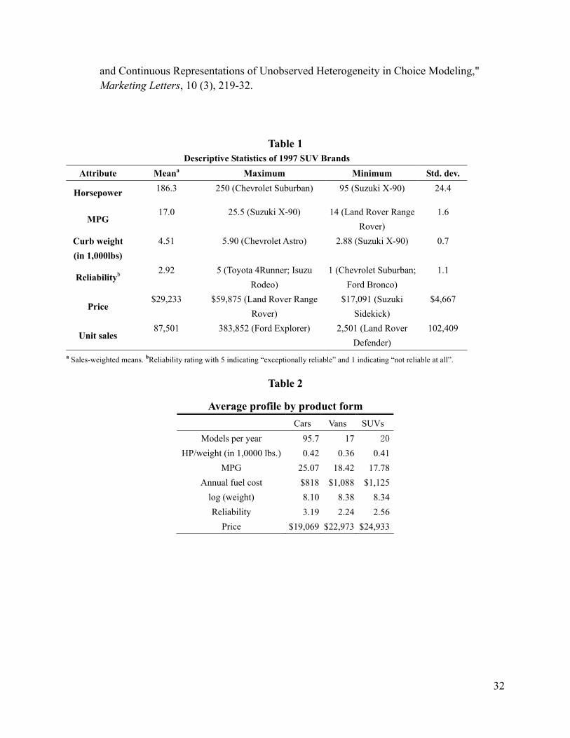
Table 1 presents descriptive statistics for SUV brands in the 1997 model year. As seen from the

table, the Chevrolet Suburban has more than twice the horsepower (250) as the Suzuki Sidekick

(95) and the Land Rover Range Rover costs 3.7 times ($37,300) as much as the Sidekick

($10,650). We use a characteristics-based demand model of differentiated products (Lancaster

1971; McFadden 1973) that projects brands onto a characteristics space so that we can flexibly

account for within- and cross-form substitution of the products.

Finally, the model needs to allow for heterogeneity in consumers’ preferences for product

attributes and the rates at which their preferences for alternative product forms change over time.

The heterogeneity allows us to account for differences in when consumers adopt the new product

form. A number of studies, such as Jensen (1982), Oren and Schwartz (1988), Chatterjee and

Eliashberg (1990), Horsky (1990), and Song and Chintagunta (2003) have formulated micro-level

models of adoption timing. In contrast with these models that focus on a single product, our

model incorporates substitution effects in the choice for product forms. We account for both

unobserved heterogeneity as well as observed heterogeneity by explicitly allowing for

interactions between demographics and category preferences (e.g. Gupta and Chintagunta 1994).

By making use of a longitudinal household-level National Household Transportation Survey data

set, we are able to infer market structure for different consumer segments over time. We find that

demographics helps explain and predict the preference for sport-utility vehicles, consistent with

Fennell et al.’s (2003) finding that observed consumer characteristics aid in predicting category

choice.

In summary, the three core components of our model are: (1) time-varying substitutability

among product forms, (2) a characteristics-based structure for brand differentiation, and (3)

heterogeneity in consumer preferences and adoption rates for the new product form. By

incorporating these three components simultaneously, we are able to (i) identify the trends in

7

own- and cross-brand price elasticities for each product form in the market, (ii) identify the

evolution of product-form substitutability, (iii) represent time-varying market structure at the

level of the aggregate market, as well as at the level of consumer segments.

3. The econometric model

3.1. Utility specification

Most previous studies on time-varying marketing mix effects or market structure use sales

response models such as the log-log models (e.g., Parker 1992; Simon 1979; van Heerde et al.

2004; van Heerde et al. 2000) that are calibrated on store-level or market-level data. The key

benefit of the log-log sales model is that price elasticities can be conveniently parameterized and

directly estimated in the regression. However, this approach is not very appealing for our research

purposes. First, when there are a large number of brands in the market under investigation,

estimating all the cross-brand price elasticities within a log-log framework is often empirically

infeasible. For example, the automobile market consists of over 130 differentiated brands, which

would require parameterizing at least 1302 own- and cross-price effects in a sales model even if

elasticity dynamics are assumed away. Second and more importantly, as mentioned earlier, the

sales model does not incorporate consumer heterogeneity, which is crucial to understanding how

substitution occurs within and between product forms for different segments of the market. We

use a characteristics-based discrete choice model of household demand to resolve these two

issues. Projecting the brand space onto a space of brand attributes solves the dimensionality

problem, and incorporating observed and unobserved consumer characteristics in the utility

function allows for heterogeneity.

The demand function is derived from household-level utility-maximizing behavior. The

model primitives are product attributes and household characteristics. In each period t, household

i chooses from Jt market offerings of F partially substitutable product forms. These product forms

are comparable in a K-dimensional attribute space, χ , but are also characterized by form-specific

(probably non-quantifiable) characteristics. As a new product form is introduced into the market,

consumers are likely to evaluate it both in terms of comparable attributes with existing forms and

8

in terms of its unique benefits. For instance, a household’s decision to purchase a sport-utility

vehicle may be either attributed to the fact that the household members find the measurable

attributes of the vehicle model (such as horsepower, acceleration, cargo space, and reliability)

better satisfy their needs relative to other products available on the market, or that they like its

four-wheel drive capacity, its higher-view-of-the-road, or the image of “ruggedness” that a SUV

uniquely embodies for them.

We use a random coefficients multinomial logit specification (RC-MNL) to model the

individual choice (Gonul and Srinivasan 1993; Jain et al. 1994; McFadden and Train 2000). As

shown in previous work, the random coefficients free the model from the unrealistic IIA property

of the simple multinomial logit model and allow for flexible substitution patterns.

Formally, the conditional indirect utility derived by household i for purchasing brand j

that has form ( )f j at time t is given by

( )( , , , ; ) ( )jt jt it jt t if j t jt it i it jt jt ijtU x p x g y pτ ξ θ φ β ξ ε′= + + − + + (1)

where jtx is a K-dimensional vector of observed product attributes of brand j at time t, jtp is

the real price of brand j, 1 2( , , )it it it itD v vτ ≡ is a vector that includes both the household i’s

observed demographic characteristics ( itD ) and other unobserved characteristics 1 2( ( , ))it it itv v v= .

We discuss the two sets of unobserved characteristics subsequently. jtξ is the econometrically

unobserved quality component of product j at time t, probably due to brand reputation, prestige,

national advertising, etc. tθ is the parameter vector to be estimated. iftφ is household i’s

preference for product form f at time t. itβ is a K-dimensional vector capturing household i’s

preferences for the K observed attributes. ity is the real income of household i at time t and is

part of the demographic profile vector itD . ( )ig ⋅ is a function capturing the household’s utility

from the remaining budget after purchase. Even though heterogeneity in marginal effects of price

9

are partially accounted through the observable heterogeneity in income, similar to Petrin (2002),

we allow the marginal utility of income to also depend on income levels:

1 ,

2

( ) ln( )

if quantile( ,0.667);where ( )

otherwise.

i it jt i it jt

it y ti it

g y p y p

y Fy

α

αα α

α

− = −

≤≡ =

(2)

where ,y tF is the population distribution function of income at time t. In other words, we use the

66.7 percentile to divide the household incomes in a given year into two groups2. ijtε is an

idiosyncratic preference shock, which is assumed to be identically and independently distributed

Type I extreme value across households and alternatives.

Similar to most previous RC-MNL models, we allow the taste parameters, 1 1({ } ,{ } )tFKikt k ift fβ φ= = ,

to vary across households. However, previous choice models generally ignore temporal changes

in taste parameters. Even though the models are calibrated on either panel or time-series data

over a relatively long period of time, they restrict parameters to be constant over the entire

sample period (for example, Berry et al. 1995; Petrin 2002). While the assumption of

time-invariant tastes may be a reasonable approximation in stable markets over a relatively short

period of time, it is most likely to fail in evolving markets such as one where a new product form

such as the SUV gradually gains acceptance from consumers. By assuming time-invariant

parameters in such markets, we may overlook significant trends, which can result in flawed

marketing strategies.

We model household i’s time-varying preferences for alternative product forms, iftφ , in the

following fashion:

1 1 2, (0, );ift ft ft it ift ift fD v v Nφ φ ς′= +Π + ∼ (3)

2 We initially followed Petrin (2002) and used the 33.3 and 66.7 quantiles to divide the vehicle-owning population into three

equally sized groups, but we did not find significant difference between the estimated price coefficients for the two lower-income

groups. Therefore, we grouped the two lower-income groups together, and the results reported here are estimated on the

two-group specification. We also experimented with the 50 and 75 percentile threshold and found the 66.7 threshold seemed to fit

the data best.

10

where itD is a D-dimensional vector capturing the demographic profile of household i at time t ,

ftΠ is D-dimensional vector of parameters that capture the relationship between demographic

characteristics and preference for product form f, and 1iftv is the f-th element of 1

itv . Further, we

specify , 1ft f t f fttrφ φ η−= + + where , 1ft f t ftη ρ η κ−= + , and 2(0, )ft Nκ ι∼ . Setting ,0 0fη = as

the initial condition, the above specification implies that ( )

1

01

(1 )

1j

t stf s

ft f fs

t trκ ρ

φ φρ

− +

=

−= + ⋅ +

−∑ .

The above specification allows the mean preferences for form f to have both a linear trend

and first-order serial correlation. The coefficient characterizing the serial correlation, ρ , can be

either positive or negative. For example, category-level advertising carryover effect tends to

imply 0ρ > . On the other hand, if a manufacturer uses unobserved rebates to merely temporally

shift consumers’ purchases from next period, this would imply 0ρ < . We capture any potential

trends in preferences forms using the trend parameter ftr . We experimented with other

polynomial specifications for the trends and did not find any significant evidence for

non-linearity in the trend terms.

Note that we allow the interactions between demographics and product form preferences

( ftΠ ’s) to be time-varying, which implies that a given household’s preferences for various

product forms may shift over time, even if the household’s covariates remain unchanged.

Identifying the dynamics in such interactions would be of considerable value to marketers to

analyze and design customer segmentation and targeting strategies. For example, what are the

characteristics of the consumers who have shifted from minivans to sport-utility vehicles? Do

they tend to be more or less affluent? Do they have larger or smaller families? What stages of

family life cycle do they tend to be in? In a market where substitution between product forms is a

major phenomenon, one must take into account consumer heterogeneity and its impact on

product-form choice in order to answer such questions.

We allow for both observed and unobserved heterogeneity for household i’s taste vector for

11

the kth product attribute, iktβ , which is assumed to take the following form

2 2 2, (0, )ikt k k it it it kD v v Nβ β σ= +Λ + ∼ (4)

Note that, unlike our specification for the product-form preferences, the mean tastes for attributes

and the interaction terms between attribute tastes and demographics are assumed to be constant

over time. We believe that these parameters tend to reflect the consumer’s inherent preference for

product features and are thus less likely to be affected by the diffusion of a new product form.

Since we use a nine-year time framework in our empirical study, we do not expect these

parameters to change significantly.3

In this discrete choice model, each household is assumed to buy one product that gives the

highest utility. Household i may not purchase any of the products within the F product forms

and this no-purchase option is accommodated by allowing for an outside good that offers utility

0 0 0 0 0( , ; ) ( )t it t i it t i t i tU g y vξ τ θ ξ ς ε= + + + (5)

where 0i tε is distributed i.i.d. extreme value. Our empirical study is concerned with the new light

vehicle market, so the outside good for a household may include continuous use of currently

owned vehicles, purchasing used vehicles, and utilizing public transportation.

Since the choice probabilities derived from the multinomial logit choice model only depend

on utility differences 0( )ijt ijt i tu U U≡ − with respect to the outside good, 0tξ cannot be

identified separately from ftφ ’s. Also 0ς cannot be identified separately from 1{ }Ff fς = ;

therefore, we normalize 0ς to be 1 and identify 1{ }Ff fς = through a Cholesky decomposition of

the resulting variance-covariance matrix after differencing:

3 As a robustness check, we estimated another specification with two separate β ’s: one for the 1991-1995 period, the other for

the 1996-1999 period. No significant difference was found in the estimated coefficients but efficiency was substantially

compromised. Therefore, we keep the specification in eq. (4) in reporting the final results. It is reasonable to question whether

consumer sensitivity to fuel efficiency will not vary over time in response to the cost of gasoline. For this variable, we use the

annual fuel cost for the vehicle, rather than the miles per gallon measure of fuel efficiency directly.

12

21

22

1

2

1 1 11 1

11 1 1 F

ςς

ς

+

+ Σ = +

(6)

We partition the household i’s utility conditional on purchasing brand j at time t, relative to

the utility derived from the outside alternative 0( )ijt ijt i tu U U≡ − , into 1( , , ; )jt jt jt jtx pδ δ ξ θ≡ and

2( , , ; )ijt jt jt itx pµ µ τ θ≡ , where jtδ is the brand-specific mean-utility component that does not

rely on household characteristics, and ijtµ is the household i’s deviation from the mean that

depends on household characteristics.

1 2( , , ; ) ( , , ; )ijt jt jt jt jt jt it ijtu x p x pδ ξ θ µ τ θ ε= + + (7)

where ( )

1

1

(1 )

1j

t stf s

jt jts

κ ρξ ξ

ρ

− +

=

−≡ +

−∑ is the error term in 1( , , ; )jt jt jtx pδ ξ θ . Here, we decompose

the parameter set into two 1 1 0, 1({ } ,{ , , } , )K Fk k f f f ftrθ β φ ρ ι= =≡ , and 2 1 2 1( , , , , ,{ } )T

tθ α α σ ω =≡ Λ Π ,

where 1θ reflects the parameters that affect the mean utility of the brand and 2θ are parameters

that capture heterogeneity in consumer preferences. Partitioning the parameter space in this

fashion has important implications for estimation, which we will discuss in the next section on

estimation.

3.2. Household choice probability

The household is assumed to choose the alternative that offers the maximum level of utility;

that is, for any i, j and t:

1 21 if max{0, , ,..., }

0 otherwisetijt i t i t iJ t

ijt

u u u uy

==

(8)

Given the distributional assumption on the idiosyncratic error terms, ijtε , the expected choice

probability of household i for brand j at time t is given by the integral

13

1

exp( ( ))(x ,p ,ξ , ; ) ( )

1 exp( ( ))t

jt ijt itijt t t t it vJv

lt ilt itl

vs D dF v

v

δ µθ

δ µ=

+=

+ +∫

∑ (9)

Since equation (9) does not have an analytical form for general distributional families of

( )vF ⋅ , it is replaced in estimation by an unbiased simulation estimator4

1

1(x ,p ,ξ , ; ) (x , p ,ξ , ; , )R

R rijt t t t it ijt t t t it it

rs D s D v

Rθ θ

=

= ∑ (10)

where ritv is the r-th random draw from the unobserved heterogeneity distribution ( )vF ⋅ .

3.2. Aggregate demand

We derive the market shares by integrating the household-level choice probabilities over both

the observed and unobserved household characteristics

2(δ ( ), , , ; ) ( , , , , ) ( ) ( )jt jt t t t D ijt t t t it it v DD vs s x p F s x p D v dF v dF Dθ ξ≡ ⋅ = ∫ ∫ (11)

In general, the integral in (11) does not have an analytical form, so we replace the inner

integral with (x , p ,ξ , ; )Rijt t t t its D θ , the simulated household-level choice probabilities and

aggregate them over the sample of households from the NPTS data set

( , , , ; )Rjt ijt t t t it

is s x p Dξ θ=∑ (12)

4. Data and Estimation

4.1. Data

The market-level data used in the empirical study includes the brand-level information of the

U.S. light vehicle market from 1991 to 1999. Model characteristics (such as horsepower, miles

per gallon, weight and manufacturer) and sales are collected from the Ward’s Automotive

Yearbook for model years from 1991 to 1999. The data on annual fuel cost estimates are

collected from the U.S. Environmental Protection Agency (EPA) website5. Reliability ratings are 4 In the empirical implementation, we use a frequency simulator with 120 Halton draws per household. Train (2001) and Bhat

(2003) show that using draws from Halton sequences, as compared to random draws, vastly reduces simulation errors and

computational burden in mixed logit models.

5 http://www.epa.gov/otaq/fereport.htm.

14

published in the annual special issues of Consumer Reports. Prices are deflated using consumer

price indices published in the Statistical Abstracts. Table 2 presents the number of brands and

average vehicle characteristics by product form. Also, it is easy to notice that the average price

for a sport-utility vehicle is highest among all product forms. In this study, we identify passenger

cars, vans, and sport-utility vehicles as three partially substitutable forms. Although there are

often multiple size-classes within each of these product form, such differentiation is typically

quantifiable and can be captured by brand attributes such as size and curb weight.6

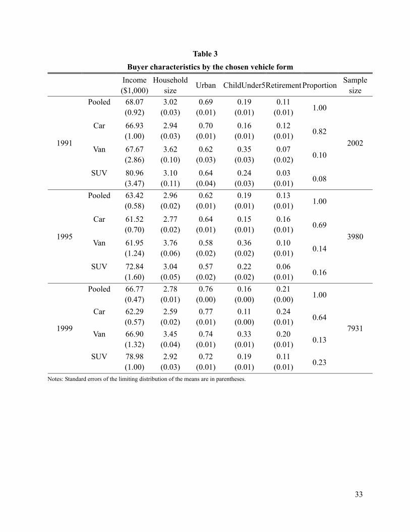
The household-level information is collected from the Vehicle Files of National Household

Transportation Survey (NHTS), a comprehensive survey conducted by the Federal Highway

Administration (FHWA), roughly once every 5 years. For each household in the survey, the

model-year of each vehicle operated by the household, and the vehicle purchase status (new vs.

used) and time are reported, together with household characteristics. We only include the

households that purchased a new car, van, or SUV, in the model year 1991, 1995, or 1999 in this

study7. The demographic variables used in our study include: household income, household size,

an urban/rural dummy, and two dummy variables of family life-cycle (whether the household has

a child under 5, and whether the household head is retired). Table 3 describes the average

6 Since we focus on the light vehicle market, medium-duty (Class 4 -7) and heavy-duty (Class 8) trucks are excluded from the

study by definition. Pickup trucks, which are typically designed with a small cab with a single row of seats and a separate open

box area for cargo, are also excluded because of their emphasis on the cargo-hauling function instead of the human-carrying

function, which makes it inappropriate to directly study the substitution between pickup trucks and other light vehicle forms (cars,

vans, and SUVs) for the family vehicle choice. Nevertheless, since the year 2000 automakers have introduced a number of new

pickup models characterized by extended cab area, four-door design, and luxury interiors (such as the Chevrolet Escalade EXT

and Toyota Tundra), making them potentially trendy alternatives for family vehicles (Kerwin 1999). However, this emerging

trend is still not significant in the industry and it is beyond the sample period of our study. 7 The data is compiled from the NPTS surveys conducted in 1990, 1995, and 2001. In the 1990 survey, a majority of the new

vehicles purchased was labeled with the model year 1991 and thus can be used as a sample of the 1991 vehicle model purchases.

The 1999 vehicle purchase data are recovered from the 2001 survey, which might induce certain missing observations: for

example, if a household that bought a new vehicle in 1999 sold it before 2001, the 1999 purchase is not reported in the data.

However since we expect most households to keep a car for at least two years, we do not believe that this has a serious effect on

our sample. If we had data on other years, we would very easily include data from other years into the study within the general

framework discussed here.

15

household profile by the chosen product form.

To convert sales quantities to the market shares to be used in the estimation, we need

knowledge of the total market size, which also consists of the demand for the outside good. We

use the number of licensed drivers in the U.S. divided by the average vehicle age to approximate

the total market size of cars in any given year.

4.2 Estimation

Theoretically, if longitudinal household-level information is available, a maximum

simulated likelihood (MSL) estimator can be used with brand-period fixed effects. Without these

fixed effects, there will be endogeneity concerns. However, there are at least two difficulties in

estimating the market structure using SML with merely household-level data. First, the

optimization procedure associated with SML has to search over a very large parameter space of

these fixed effects, and the dimensionality problem makes convergence practically impossible.

Second, unless the sample is extremely large, household-level data is unlikely to serve as a

reasonable approximation to the market shares of the hundreds of brands in the auto market and

hence can lead to highly imprecise estimates of market structure at the brand level.

Aggregate data can improve the efficiency of estimators when used in combination with

individual-level data (Imbens and Lancaster 1994). Because the aggregate information provides

the average of a microeconomic variable with very small sampling error, it virtually constitutes

an additional constraint in the conditional maximum likelihood estimation and reduces the

asymptotic variance of the estimator. In our case, the observed market shares can be viewed as

accurate estimates of the average household choice probabilities, and incorporating such

information will serve to reduce sampling error and improve efficiency. We therefore combine

the disaggregate information with market-level information to estimate the model.

Given the difficulties in employing likelihood-based estimation, we use a generalized

method of moments (GMM) framework for estimation. Specifically, we generate moment

conditions both from the household-level data and from the market-level data for estimation.

For the aggregate data, we follow Berry et al.’s (1995) approach to generate moment conditions.

16

We assume that the demand-side error ξ is orthogonal to a set of exogenous instrumental

variables. Formally, for any j and t, the following conditions hold

0[ ( ) ] 0jt jtE zξ θ ′ = (13)

where jtz is a L -dimensional vector of instruments, , and 0θ is the true parameter vector that

governs the data generating process.

We assume that the error term is exogenous to all observed product attributes ( , ( ))jtx f j

and trends; however, other instruments are required to resolve the endogeneity of the price

variable. Since the econometrically unobserved product characteristic, jtξ , is likely to be

observable to consumers and price-setting oligopolistic firms, it is probably correlated with prices

and creates an endogeneity problem. Not properly resolving the endogeneity issue can lead to

downward bias of the price coefficients; further not taking into account the unobservable product

characteristics creates an econometric over-fitting problem (e.g., Berry et al. 1995). To deal with

endogeneity and over-fitting, we draw upon the contraction mapping scheme proposed by Berry

(1994) to facilitate linear instrumental variable estimation. Berry established that under mild

regularity conditions, there exists a unique mean utility vector, 2( )δ θ , that equates the predicted

market shares in (14) to the observed market shares. An iterative procedure is used to solve for

2( )δ θ :

( 1) ( ) o ( )2 2 2 2( ) ( ) ln(s ) ln( ( , , ( ) , ; ))h h h

Ds p x Fδ θ δ θ δ θ θ+ = + − (14)

where os is the vector of observed market shares, and ( )2 2( , , ( ) , ; )h

Ds p x Pδ θ θ is the vector of

predicted shares conditional on ( )2( ) hδ θ and 2θ . The procedure is iterated until convergence.

2 2 ( ),0 ( )( ) ( ) ( )jt jt jt f j f jx t trξ θ δ θ β φ′= − − + ⋅ (15)

Then the instrumental variable approach is used to obtain consistent estimators for

,0 1( ,{ , } )Ff f ftrβ φ = , and a second-stage differencing is applied to the fitted residuals ˆ

jtξ to obtain

17

estimates for ( , )ρ ι . We construct four sets of instruments, including the observed characteristics

of the product and a function of the characteristics of other products as an approximation to the

equilibrium first-order conditions: (1) the product’s own physical characteristics, (2) the average

within-firm, same-form characteristics (excluding those of the product itself), and (3) the average

without-firm same-form characteristics, and (4) the average same-country-of-origin same-form

characteristics. (See, for example, Berry et al. 1995 and Sudhir 2001 for a motivation of these

instruments)

Conditional on 2θ , the sample moment for the aggregate data is

1 2 2 2( ) ( ) ( )jt jt jt jtG z Wzθ ξ θ ξ θ′′ ′= (16)

where 2( )jtξ θ is the residual from the instrumental variable estimation of eq. (15), and W is a

symmetric, nonnegative definite weight matrix.

Since the household-level decisions are observed in the micro data, we can construct

moment conditions similar to those used for the method of simulated moments (MSM) estimator

for individual-level data (e.g. McFadden and Train 2000; Wedel et al. 1999) that minimizes the

objective function

2 ( ) ( (x ,p ,ξ , ; ))Rijt ijt ijt t t t it

t i jG w y s Dθ θ= −∑∑∑ (17)

where ijtw is a vector of instrumental variables that are orthogonal to the errors in the population,

and (x , ,p ,ξ , ; )Rijt t t t t its d D θ is as defined in eq. (10). McFadden (1989) established that under

mild regularity conditions the MSM estimator is consistent and asymptotically normal. When the

instruments equal the scores, 0ln (x ,p ,ξ , ; )ijt t t t its D θ θ∂ ∂ , then the MSM estimator coincides

with the MSL estimator and becomes fully efficient. Therefore, an intuitive approach to

generating these instruments would be to compute the simulated scores,

1

1 ln (x ,p ,ξ , , ; )R

rijt t t t it it

rs D v

R θ θ=

∇∑ .

To reduce the dimensionality issue involved in the computation of the simulated scores, we

18

use the mean utility vectors obtained from eq. (14) to compute the gradient of

2 2ln ( ( ), , , ; )ijt t t t its x p Dδ θ θ with respect to 2θ :

1 11 1

ln 1 1 ( )R J

ijt ijt r rjkt ik ilt lkt ik

r lk ijt k

s sx v s x v

s Rσ σ = =

∂ ∂= = −

∂ ∂ ∑ ∑

2 ( ) 2 ( )1 1

ln 1 1 ( )R J

ijt ijt r rif j ilt if j

r lf ijt f

s sv s v

s Rς ς = =

∂ ∂= = −

∂ ∂ ∑ ∑

1

ln 1 Jijt ijt

jkt it ilt ilt itlk ijt k

s sx D s x D

s =

∂ ∂= = −

∂Λ ∂Λ ∑ (18)

1

ln 1 Jijt ijt

it ilt itlf ijt f

s sD s D

sπ π =

∂ ∂= = −

∂ ∂ ∑

1

ln 1 1( )J

ijt ijt ilt

li ijt i it jt it lt

s s ss y p y pα α =

∂ ∂= = − −

∂ ∂ − −∑

We then set 2 2 2ln ( ( ), , , ; )ijt ijt t t t itw s x p Dδ θ θ θ= ∂ ∂ in eq. (17) for each 2θ .

Combining the macro and micro moments, we have the combined moment conditions

1 22

2 2

( )( )

( )G

GG

θθ

θ

=

(19)

Following Hansen (1982), the efficient GMM estimator is defined as 1ˆ arg min ( ) ( )GMM G V G

θθ θ θ−

∈Θ′= (20)

where 1V − is a weighting matrix that satisfies 0 0plim [ ( ) ( ) ]V E G Gθ θ ′=

The asymptotic variance of the GMM estimator is then given by d

1 1GMM 0ˆ ( - ) (0, ( ) )n N Vθ θ − −′→ Γ Γ (21)

where 0[ ( ) ]E G θ θΓ = ∂ ∂ , which is approximated by its consistent estimate inferred from the

first-stage estimation.

The estimation procedure is summarized as follows:

(1) Make R draws from the unobserved heterogeneity distribution over itv for each

19

observation (and fix these draws throughout the iterations).

(2) Pick an initial value (0)2θ ;

(3) For the h-th iteration, conditioning on ( )2

hθ , compute ( ) ( )2(s , )h h

jt jt tδ δ θ≡ by matching the

predicted market shares with the observed market shares as sketched in eq. (14);

(4) For each household in the micro data, compute ( ) ( ) ( )2( , , )h R h h

ijt ijt jt its s Dδ θ≡ , the simulated

individual choice probability, and 2

( ) ( ) ( )2( , ; )h R h h

ijt ijt jt itw s Dθ δ θ= ∇ using eqs. (18);

(5) Compute 1 2( )G θ in eq. (16) and 2 ( )G θ in eq. (17);

Compute the GMM objective function using eq. (19) and search for the value of 2θ that

minimizes the objective function through iterations.

We note that Petrin (2002) augments market-level data by constructing additional moments

in terms of observable average buyer demographics using household-level survey data. This

approach of creating aggregate market shares at the aggregate level is inefficient when the data

are available at the household level, and cannot provide us adequate degrees of freedom to

estimate time-varying preferences in inferring market structure dynamics.

Our unified GMM approach is different from Dube and Chintagunta (Chintagunta and Dube

2004; 2004) who also estimate a model that combines household data with store-level aggregate

data. In their approach, they use maximum likelihood on the household data to identify

heterogeneity and GMM on the aggregate store-level data to identify the mean utility levels and

iterate over the two stages to obtain convergence. Further, in contrast to our time-varying utility

model of demand, they estimate a time-invariant utility model of demand. 4. Estimation Results

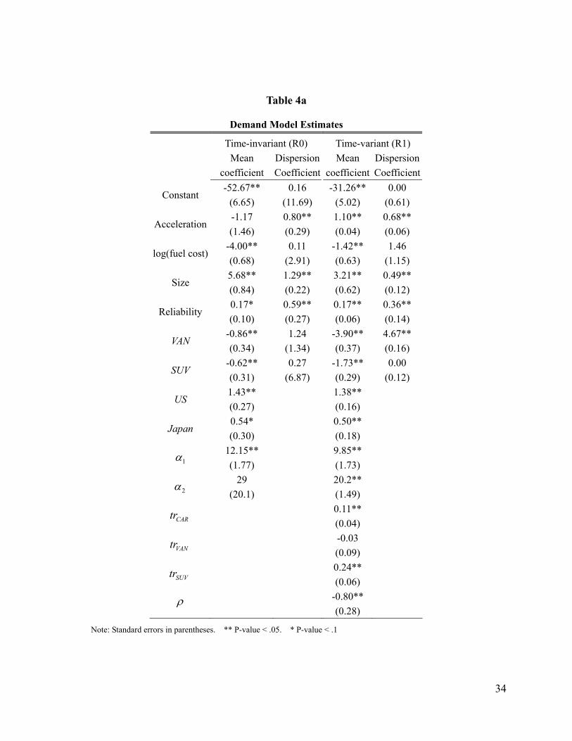
Tables 4a and 4b present the estimation results of the demand models. Table 4a presents the

estimates for the mean and dispersion coefficients for both the time-invariant and time-variant

specifications. Table 4b presents the estimates for the interaction parameters between household

demographics and category preferences. The time-invariant specification (R0) assumes

20

time-invariant preferences and demographic interactions, so only one set of interactions, Π≡Π t ,

is estimated. For the time-variant specification (R1), we estimate three sets of interactions, for the

years 1991, 1995, and 1999, when the household-level data is available. For the intervening years,

we use a linear interpolation between the estimates for the closest years.

As seen in Table 4a, for both specifications, the mean coefficients for attributes ( β ) are all

significant. The market, as a whole, prefers larger, higher-quality, and fuel-efficient vehicles.

Consumers on average prefer domestic vehicles to imports. The dispersion coefficients ( kσ ’s) are

all significantly different from zero, except for fuel efficiency. The category preference dispersion

( fς ) is virtually zero for cars and SUVs, yet is large for vans. The time-variant model identifies a

significant trend in preferences favoring the SUV. The autoregressive coefficient ( ρ ) is estimated

to be negative (as in the homogeneous logit model) suggesting that purchase timing effects

(induced by manufacturer’s rebates, for example) dominate potential advertising carryover

effects.

In Table 4b, the first two columns present the results from the time-invariant specification. It

is evident that household size has the most impact on the preference for vans, whereas income is

the most influential factor in the preference for SUVs. Urban dwellers prefer cars to vans and

SUVs. Retirees favor vans most and favor SUVs least. Families with young children prefer vans

and SUVs to cars, though the preference for vans is much greater. Note that the interaction terms

do not remain constant over time, and, furthermore, such interactions may have nonlinear

patterns over time. Table 5 presents the average partial effects of demographics on vehicle form

choice. For instance, a 1% increase in household income increases the household’s probability of

purchasing a SUV by 0.55% in 1991 while the corresponding increase is 0.43% in 1995 and

0.48% in 1999. Household size has a decreasing effect on SUV preference while having an

increasing effect on van preference. A test against the time-invariant model (R0) rejects the null

(F=19.49, p<.05), indicating the need to incorporate time-varying preferences and interactions in

this market.

21

5. Market structure dynamics

5.1. Price Elasticities

As a first step towards understanding market dynamics, we investigate how own-brand

price elasticities change over time. Researchers have argued that price elasticities increase over

time because of increased competitiveness and consumer knowledge as an industry matures.

Tellis (1988) finds support for this hypothesis through a meta-analysis of over 200 brands. On the

contrary, Simon (1979) finds that brand-level price elasticity trends can be non-monotone: they

initially decline and then rise in the mature stage for the detergent and pharmaceutical categories.

Table 6 presents the regression results of how own-brand price elasticities (in absolute terms)

for the three vehicle forms change over time. We find a significantly positive trend in

own-elasticity for cars and SUVs, but a negative trend for vans. The positive trend for cars and

SUVs suggest that perceived brand differentiation among vehicles in each group is diminishing

for consumers. The magnitude of the trend for SUVs is especially large, suggesting that the SUV

category became increasingly crowded with highly substitutable brands. In contrast, the

significantly negative trend for vans, suggests increasing brand differentiation and lower

competitive pressure among vans. van Heerde et al. (2004) find that an introduction of an

innovative pizza brand caused other brands to be perceived as less differentiated. Interestingly,

we find that the introduction of a new product form (SUV) can have opposing effects on the two

existing forms: while vans became more differentiated, cars became less differentiated.

5.2. Brand-level market structure

“Clout” and “vulnerability” are two well known metrics used to represent a brand’s

competitive position and has been used to study market structure (Chintagunta 2002; Kamakura

and Russell 1989; van Heerde et al. 2004). The competitive clout measure captures the impact of

a brand on the sales of other brands and is defined as

1Competitive Clout: C ( )jt jkt kt ktk j k jjt

s sn

η≠ ≠

=∑ ∑ (22)

where kjtη is the elasticity of brand j’s market share to brand k’s price at year t, kts is the

22

market share of brand k at time t. The denominator is the mean share of the competing brands

included in the numerator. Our measure of clout is similar in spirit to the measures used

previously. The difference is that the above measure weights the cross-brand elasticities by

market share rather than simply take the summation of elasticities. The unweighted clout measure

may work well for a category with a small number of brands where shares are roughly similar;

however, when the number of brands and differences in market shares are both large as in the

auto market, the unweighted measure is not representative of clout because it over-weights the

elasiticities of small-share brands disproportionately. The vulnerability measure, which captures

the impact of price changes of all other brands on the sales of the focal brand, is the same as in

van Heerde et al. (2004). Here market share weighting is not required because the market share

effect is measured only for the focal brand j.

Vulnerability: V =jt kjtk jη

≠∑ (23)

where kjtη is the elasticity of brand j’s market share to brand k’s price at year t.

We compute these two metrics for each vehicle brand and perform ordinary least squares

regression on a product form dummy and a time trend. The regression results are reported in

Table 7. For cars and SUVs, both clout and vulnerability significantly increased from 1991 to

1999, suggesting a larger degree of brand-level substitutability over time. For vans, however, no

such increase in clout and vulnerability is found: the trends are estimated to be negative but not

significant. This finding is consistent with the pattern found in the analysis of own-brand

elasticities.

5.3. Form-level measures of market structure

Given our interest in how the introduction of a new product form affects market structure and

competition with other existing product forms, we develop summary measures of competition

across product forms. Table 8 presents the estimates for product-form-level elasticities, with

,ff tη ′ indicating the percentage change in the total share of product form f with one percent

change in the prices of all brands of product form f ′ . The SUV seems to be the most elastic

23

among all three groups, with overall elasticities of about 0.89, and the passenger car category is

the most inelastic among all, with relatively stable elasticity around 0.15. Suppose a 1% tax is

imposed on all SUV brands (say, due to their high fuel consumption or lower emission standard),

SUV demand will drop by 0.89%, while demand for cars increase by 0.11% and demand for vans

increase by 0.30%.

We also decompose each of the clout and vulnerability metrics into an intra-form

component and an inter-form component.

,,, ,

mean ( ) , if , C

mean ( ) , otherwise.

jkt kt ktk j k fk j k fj f t

jkt kt ktk fk c

s s j f

s s

η

η

≠ ∈≠ ∈

∈∈

∈=

∑

∑ (24)

,, ,

, if , V

, otherwise.

kjtk j k f

j f tkjt

k f

j fη

η≠ ∈

∈

∈

=

∑

∑ (25)

where , , C j f t and , , Vj f t are the clout and vulnerability, respectively, of brand j with respect to

product form f at year t. We regress these measures on category dummies and time trends to

understand the dynamics of form-specific market structure. We show these results using Figure 2.

Figure 2a, shows the clout and vulnerability of cars, vans and SUVs with respect to cars. Figures

2b and 2c show the same with respect to vans and SUVs, respectively. The vulnerability of form i

with respect to form j is the impact of the price change by vehicles of form j, on the market share

of the form i. The clout of form i with respect to form j is the impact of the price change by a

vehicle of form i, on the market share of the form j. The start (end) of the arrow in the maps

indicates 1991 (1999). All non-zero slopes indicated in the graphs have trend coefficients with at

least 95% statistical significance.

As is seen in Figure 2a, intra-form substitution (among cars) is the primary source of

competitive pressure for cars; also, a pricing discount on one car brand is most likely to

negatively affect the sales of other car brands rather than grab shares from other product forms.

The intra-form competition among cars increased about 30% from 1991 to 1999, and the

own-brand price elasticity (in absolute value) also increased substantially during the sample

24

period, suggesting a diminishing brand differentiation in consumers’ perception of car brands.

The average van brand possessed a relatively large competitive clout over cars in the early 90s,

but the influence declined over time and reduced by half towards 1999. On the contrary, the

competitive clout of an average SUV brand on cars increased tremendously; by 1994, the

competitive clout of SUVs on the car category had taken over that of vans, indicating an

increasing substitutability between cars and SUVs. SUVs also gained an advantageous

competitive position with respect to cars over time, as indicated by their increasing competitive

clout.

Figure 2b plots the competitive clout and vulnerability measures of an average car, van, or

SUV brand with respect to the van category. As with cars, the van category, competition among

vans (intra-form substitution) is the major source of competitive pressure; but the intra-form

competitiveness among vans decreased over time, as opposed to the increasing trend for cars. An

average van brand became less vulnerable to pricing cuts by other vans, which is consistent with

our previous finding that the own-brand elasticity actually decreased (in absolute terms) in the

van category and suggests larger perceived brand differentiation within this category. However

cars and vans appear to be poor substitutes, i.e., an average car brand has minimal clout on the

van category and is not much affected by van prices. In contrast, SUVs compete much more

closely with vans. While SUVs gained competitive clout over vans during the sample period, its

vulnerability with respect to vans declined.

While intra-form substitution was the major source of competitive pressure for cars and

vans throughout the data period, inter-category substitution was the major contributor of

competitive pressure for SUVs in 1991. Vans had a large clout on SUV sales in the early 90s. But

the clout of vans declined, and intra-form pricing competition among SUVs became the more

dominant source of competition for SUVs by 1999.

An interesting finding is that in the early nineties, SUVs competed more closely with vans,

but by the late nineties SUVs competed more closely with cars. This empirical result is consistent

with the positioning of SUVs over the sample period by auto firms as reported widely in the trade

press. Detroit-based automobile makers positioned the SUV as the “anti-minivan” (the stylish

25

alternative to minivans) in the late eighties and early nineties, but by the mid-nineties began to

position it against cars as a “lifestyle” vehicle which combines the comfort of a car with the

functionality of a truck.

5.3 Market structure by consumer segments

Given the richness of the micro-level NHPS data, we are able to identify the effects of both

observed and unobserved consumer characteristics in vehicle choices. This enables us to identify

dynamics in market structure across different consumer segments. We illustrate this by presenting

two sets of segment-level market structure representations. Figures 3 shows the market structure

dynamics in the same fashion as Figure 2, except we show the market structure separately for a

low and high income segment. We experimented with income thresholds of $40K, $50K, and

$60K, but did not find significant differences in the insights obtained. So, we report results based

on a $50K cutoff. Figures 3a-3c represent the market structure for the lower-income households,

and Figure 3d-3f for the higher-income households.

There are some key differences in the market structure of the high and low income segments.

For instance, a comparison between Figures 3a and 3d suggests that intra-form substitution is the

predominant competitive effect for cars in the lower-income segment; but there is significant

inter-form substitution for the higher-income segment. In particular, SUVs kept gaining

competitive clout over cars in the high income segment, while the competitive clout of vans with

respect to cars declined sharply relative to its 1991 position. Both Figures 3b and 3e illustrate that

intra-form competition is high for vans in both segments. However, Figure 3b shows shat SUVs

and vans became more substitutable for lower-income households (as indicated by the increasing

clout of SUVs over vans), whereas Figure 3e indicates that the two product forms actually

became less substitutable for higher-income households (as indicated by SUVs becoming less

vulnerable to vans over time).

The segment-level market structure maps can be insightful to marketers. To illustrate,

suppose that a firm with a major midsize car considers whether to introduce a lower-end or

higher-end SUV brand into its product line. Figures 3a and 3d suggest that the lower-end SUV

would cannibalize car sales much less compared to the higher-end SUV. This is because the

26

lower-income households find cars and SUVs less substitutable, whereas the higher-income

segment is much more likely to substitute between SUVs and cars. Also, Figures 3b and 3e

suggest that price-cutting is an effective competitive device for a SUV brand to fight against vans

for the lower-income segment, but that is not the case for the higher-income segment. Other

marketing mix instruments, such as advertising and product design, may need to be used for this

purpose for the higher-income segment.

Figure 4 shows the market structure of households segmented by household size. Figures

4a-4c are for smaller households (i.e. no more than 2 persons) and Figure 4d-4f are for larger

households (i.e. greater than or equal to three persons). The key difference in market structures

for the two segments is in the relationship between SUVs and vans. Vans lose clout and become

more vulnerable with respect to SUVs for smaller households. But intra-form substitution within

vans is still the major source of competition among larger households. Even though SUVs

gradually became a closer substitute to vans over time, a significant proportion of large

households still preferred to choose among vans.

6. Conclusion

In this paper, we propose a method to study the evolving market structure in a durable-goods

market (U.S. auto market) during a period where a new product form (the SUV) was gradually

gaining acceptance. The model incorporates changing level of product form substitutability, an

attribute level structure of brand differentiation, and observed and unobserved consumer

heterogeneity. The estimation approach combines easily collectible household level survey data

with readily available aggregate market level data and therefore can be easily implemented by

firms. We develop a unified GMM estimation approach that combines household and aggregate

data in a natural manner. The approach enables us to identify preference shifts over time and

enables us to gain insights into how product competition changes over time not only at an

aggregate level, but also across observable demographic segments. We discuss managerial

implications of our findings for both product positioning and promotional decisions. More

broadly, we argue that the inference of dynamic market structure has implications for short-term

marketing mix decisions as well as longer-term product line and R&D investment decisions.

27

While this paper stretches the frontier for dynamic market structure estimation in evolving

markets on a number of dimensions, we note some limitations in our paper which provides

interesting opportunities for future research. First, we restrict preference heterogeneity to be time

varying only along product forms, but not along specific attributes. While this appears reasonable

in our application where product attributes are fundamentally similar across product forms,

behavioral research has suggested that attribute preferences can change upon introduction of new

products. This deserves greater exploration in future research. Second, as with most market

structure studies, we model only one marketing mix variable: price. Given that consumer

preferences can be molded over time by advertising, it would be interesting as to how market

structure dynamics can be systematically affected by advertising. It may also be of interest as to

how firms compete strategically on the advertising dimension to favorably affect market structure.

Third, although we allow the consumer base of brands to change in the aggregate, we do not

model individual-level dynamics due to brand loyalty and product-form loyalty. A richer

behavioral model that accounts for consumer-level state-dependence would require a panel of

households to be included in the data set for a sufficiently long period of time (Seetharaman 2003;

Swait et al. 2004); however, such data for consumer durables are rarely collected and used for

academic research. Fourth, although it is less of an issue in the automobile market, the

forward-looking behavior of consumers may also play a role in technology-driven markets (e.g.,

Melnikov 2000; Song and Chintagunta 2003).

Finally, we hope our approach and application will spawn research in other evolving product

markets, where new product forms are constantly introduced. As we noted in our introduction, a

number of technology markets are faced with the problem of evolving market structure. We also

believe the approaches developed in this paper can be applied fruitfully in emerging markets such

as China and India, where consumer preferences for brands are evolving and new products/forms

are constantly being introduced.

28

References Belson, Ken (2004), "Teaching an Old Walkman Some New Steps," in The New York Times.

New York, NY. Berndt, Ernst R., Robert S. Pindyck, and Pierre Azoulay (2003), "Consumption Externality and

Diffusion in Pharmaceutical Markets: Antiulcer Drugs," The Journal of Industrial Economics, 51 (2), 243-70.

Berry, Steven (1994), "Estimating Discrete-Choice Models of Product Differentiation," Rand

Journal of Economics, 25 (2), 242-62. Berry, Steven, James Levinsohn, and Ariel Pakes (1995), "Automobile Prices in Market

Equilibrium," Econometrica, 63 (4), 841-90. Bhat, C. R. (2003), "Simulation Estimation of Mixed Discrete Choice Models Using Randomized

and Scrambled Halton Sequences," Transportation Research Part B-Methodological, 37 (9), 837-55.

Bradsher, Keith (2002), High and Mighty: Suvs, the World's Most Dangerous Vehicles and How

They Got That Way. New York: PublicAffairs. Carroll, J. Douglas Ed. (1972), Individual Differences and Multidimensional Scaling. New York

and London: Seminar Press. Chatterjee, Rabikar and Jehoshua Eliashberg (1990), "The Innovation Diffusion Process in a

Heterogeneous Population: A Micromodeling Approach," Management Science, 36 (9), 1057-79.

Chintagunta, P. K. (2002), "Investigating Category Pricing Behavior at a Retail Chain," Journal

of Marketing Research, 39 (2), 141-54. Chintagunta, P.K. and Jean-Pierre Dube (2004), "Estimating an Sku-Level Brand Choice Model

Combining Household Panel Data and Store Data," Working paper, University of Chicago. Conlin, Michelle (2003), "Unmarried America: Say Good-Bye to the Traditional Family. Here's

How the New Demographics Will Change Business and Society," in BusinessWeek. Consumers Union of U.S. (2004), "Cable & Satellite Tv: Which Is Better? 2004," in Consumer

Reports Vol. 69.

29

Dube, Jean-Pierre and P. K. Chintagunta (2004), "Estimating an Sku-Level Brand Choice Model Combining Household Panel Data and Store Data," Working Paper, University of Chicago.

Elrod, Terry, Gary J. Russell, Rick L. Andrews, Lynd Bacon, Barry L. Bayus, J. Douglas Carroll,

Richard M. Johnson, Wagner A. Kamakura, Peter Lenk, Josef A. Mazanec, Vithala R. Rao, and Venkatesh Shankar (2002), "Inferring Market Structure from Customer Response to Competing and Complementary Products," Marketing Letters, 13 (3), 221-32.

FCC (2001), "Federal Communications Commission Annual Assessment of the Status of

Competition in the Market for the Delivery of Video Programming," in Seventh Annual Report.

Fennell, Geraldine, Greg M. Allenby, Sha Yang, and Yancy Edwards (2003), "The Effectiveness

of Demographic and Psychographic Variables for Explaining Brand and Product Category Use," Quantitative Marketing and Economics, 1 (2), 223-44.

Gladwell, Malcolm (2004), "Big and Bad: How the S.U.V Ran over Automotive Safety," in The

New Yorker. Gonul, F. and V. Srinivasan (1993), "Modeling Multiple Sources of Heterogeneity in Multinomial

Logit Models," Marketing Science, 12 (3), 213-29. Goolsbee, Austan and Amil Petrin (2004), "The Consumer Gains from Direct Broadcast Satellites

and the Competition with Cable Tv," Econometrica, 72 (2), 351-81. Gupta, Sachin and Pradeep K. Chintagunta (1994), "On Using Demographic Variables to

Determine Segment Membership in Logit Mixture Models," Journal of Marketing Research, 31 (1), 128-36.

Hansen, L. P. (1982), "Large Sample Properties of Generalized Method of Moments Estimators,"

Econometrica, 50 (4), 1029-54. Horsky, Dan (1990), "A Diffusion Model Incorporating Product Benefits, Price, Income, and

Information," Marketing Science, 9 (4), 342-65. Howard, Bill (2003), "Ipod Competition," in PC Magazine Vol. 22. Imbens, Guido W. and Tony Lancaster (1994), "Combining Micro and Macro Data in

Microeconometric Models," Review of Economic Studies, 61, 655-80.

30

Jain, D., N. Vilcassim, and Pradeep Chintagunta (1994), "A Random Coefficient Logit Brand Choice Model Applied to Panel Data," Journal of Business and Economic Statistics, 12, 317-28.

Jensen, Richard (1982), "Adoption and Diffusion of an Innovation of Uncertain Profitability,"

Journal of Economic Theory, 27 (1), 182-93. Kadiyali, Vrinda, Naufel Vilcassim, and Pradeep Chintagunta (1999), "Product Line Extensions

and Competitive Market Interactions: An Empirical Analysis," Journal of Econometrics, 89 (1/2), 339-63.

Kamakura, Wagner A. and Gary J. Russell (1989), "A Probabilistic Choice Model for Market

Segmentation and Elasticity Structure," Journal of Marketing Research, 26 (4), 379-90. Katz, Elibu and Paul F. Lazarsfeld (1955), Personal Influence. Glencoe, Ill: Free Press. Kerwin, Kathleen (1999), "You Call This the Family Car? Pickups with Roomy Cabs Become a

Status Accessory," in BusinessWeek. McFadden, D. (1989), "A Method of Simulated Moments for Estimation of Discrete Response

Models without Numerical-Integration," Econometrica, 57 (5), 995-1026. McFadden, Daniel and Kenneth Train (2000), "Mixed Mnl Models for Discrete Response,"

Journal of Applied Econometrics, 15 (5), 447-70. Melnikov, Oleg (2000), "Demand for Differentiated Durable Products: The Case of the U. S.

Computer Printer Market," Working Paper, Department of Economics, Yale University. Moschini, Giancario (1991), "Testing for Preference Change in Consumer Demand: An Indirectly

Separable, Semiparametric Model," Journal of Business and Economic Statistics, 9 (1), 111-17.

Nair, Harikesh, Pradeep Chintagunta, and Jean-Pierre Dube (2003), "Empirical Analysis of

Indirect Network Effects in the Market for Personal Digital Assistants," Working Paper,University of Chicago.

Oren, Shmuel S. and Rick G. Schwartz (1988), "Diffusion of New Products in Risk-Sensitive

Markets," Journal of Forecasting, 7 (4), 273-87. Parker, Philip M. (1992), "Price Elasticity Dynamics over the Adoption Life Cycle," Journal of

Marketing Research, 29 (3), 358-67.

31

Petrin, Amil (2002), "Quantifying the Benefits of New Products: The Case of the Minivan,"

Journal of Political Economy, 110 (4), 705-29. Roberts, John H. and Glen L. Urban (1988), "Modeling Multiattribute Utility, Risk, and Belief

Dynamics for New Consumer Durable Brand Choice," Management Science, 34 (2), 167-85.

Seetharaman, P. B. (2003), "Probabilistic Versus Random-Utility Models of State Dependence:

An Empirical Comparison," International Journal of Research in Marketing, 20 (1), 87-96.

Simon, Hermann (1979), "Dynamics of Price Elasticity and Brand Life Cycles: An Empirical

Study," Journal of Marketing Research, 16 (4), 439-52. Song, Inseong and Pradeep K. Chintagunta (2003), "A Micromodel of New Product Adoption

with Heterogeneous and Forward-Looking Consumers: Application to the Digital Camera Category," Quantitative Marketing and Economics, 1 (4), 371-407.

Sudhir, K (2001), "Competitive Pricing Behavior in the Auto Market: A Structural Analysis,"

Marketing Science, 20 (1), 42-60. Swait, J., W. Adamowicz, and M. van Bueren (2004), "Choice and Temporal Welfare Impacts:

Incorporating History into Discrete Choice Models," Journal of Environmental Economics and Management, 47 (1), 94-116.

Tellis, Gerard J. (1988), "The Price Elasticity of Selective Demand: A Meta-Analysis of

Econometric Models of Sales," Journal of Marketing Research, 25 (4), 331-41. Train, Kenneth (2001), "Halton Sequences for Mixed Logit," Working Paper, University of

California at Berkeley. van Heerde, Harald J., Peter S.H. Leeflang, and Dick R. Wittink (2000), "The Estimation of Pre-

and Postpromotion Dips with Store-Level Scanner Data," Journal of Marketing Research, 37 (3), 383-95.

van Heerde, Harald J., Mela Carl F., and Puneet Manchanda (2004), "The Dynamic Effect of

Innovation on Market Structure," Journal of Marketing Research, 41 (2), 166-83. Wedel, Michel, Wagner Kamakura, Neeraj Arora, Albert Bemmaor, Jeongwen Chiang, Terry

Elrod, Rich Johnson, Peter Lenk, Scott Neslin, and Carsten Stig Poulsen (1999), "Discrete

32

and Continuous Representations of Unobserved Heterogeneity in Choice Modeling," Marketing Letters, 10 (3), 219-32.

Table 1 Descriptive Statistics of 1997 SUV Brands

Attribute Meana Maximum Minimum Std. dev.

Horsepower 186.3 250 (Chevrolet Suburban) 95 (Suzuki X-90) 24.4

MPG 17.0 25.5 (Suzuki X-90) 14 (Land Rover Range

Rover) 1.6

Curb weight (in 1,000lbs)

4.51 5.90 (Chevrolet Astro) 2.88 (Suzuki X-90) 0.7

Reliabilityb 2.92 5 (Toyota 4Runner; Isuzu

Rodeo) 1 (Chevrolet Suburban;

Ford Bronco) 1.1

Price $29,233 $59,875 (Land Rover Range

Rover) $17,091 (Suzuki

Sidekick) $4,667

Unit sales 87,501 383,852 (Ford Explorer) 2,501 (Land Rover

Defender) 102,409

a Sales-weighted means. bReliability rating with 5 indicating “exceptionally reliable” and 1 indicating “not reliable at all”.

Table 2

Average profile by product form Cars Vans SUVs

Models per year 95.7 17 20

HP/weight (in 1,0000 lbs.) 0.42 0.36 0.41 MPG 25.07 18.42 17.78

Annual fuel cost $818 $1,088 $1,125log (weight) 8.10 8.38 8.34 Reliability 3.19 2.24 2.56

Price $19,069 $22,973 $24,933

33

Table 3 Buyer characteristics by the chosen vehicle form

Income ($1,000)

Household size Urban ChildUnder5Retirement Proportion Sample

size Pooled 68.07

(0.92) 3.02

(0.03) 0.69

(0.01) 0.19

(0.01) 0.11

(0.01) 1.00

Car 66.93 (1.00)

2.94 (0.03)

0.70 (0.01)

0.16 (0.01)

0.12 (0.01) 0.82

Van 67.67 (2.86)

3.62 (0.10)

0.62 (0.03)

0.35 (0.03)

0.07 (0.02) 0.10

1991

SUV 80.96 (3.47)

3.10 (0.11)

0.64 (0.04)

0.24 (0.03)

0.03 (0.01) 0.08

2002

Pooled 63.42 (0.58)

2.96 (0.02)

0.62 (0.01)

0.19 (0.01)

0.13 (0.01) 1.00

Car 61.52 (0.70)

2.77 (0.02)

0.64 (0.01)

0.15 (0.01)

0.16 (0.01) 0.69

Van 61.95 (1.24)

3.76 (0.06)

0.58 (0.02)

0.36 (0.02)

0.10 (0.01) 0.14

1995

SUV 72.84 (1.60)

3.04 (0.05)

0.57 (0.02)

0.22 (0.02)

0.06 (0.01) 0.16

3980

Pooled 66.77 (0.47)

2.78 (0.01)

0.76 (0.00)

0.16 (0.00)

0.21 (0.00) 1.00

Car 62.29 (0.57)

2.59 (0.02)

0.77 (0.01)

0.11 (0.00)

0.24 (0.01) 0.64

Van 66.90 (1.32)

3.45 (0.04)

0.74 (0.01)

0.33 (0.01)

0.20 (0.01) 0.13

1999

SUV 78.98 (1.00)

2.92 (0.03)

0.72 (0.01)

0.19 (0.01)

0.11 (0.01) 0.23

7931

Notes: Standard errors of the limiting distribution of the means are in parentheses.

34

Table 4a

Demand Model Estimates

Time-invariant (R0) Time-variant (R1)

Mean

coefficient Dispersion Coefficient

Mean coefficient

Dispersion Coefficient

Constant -52.67**

(6.65) 0.16

(11.69) -31.26**

(5.02) 0.00

(0.61)

Acceleration -1.17 (1.46)

0.80** (0.29)

1.10** (0.04)

0.68** (0.06)

log(fuel cost) -4.00** (0.68)

0.11 (2.91)

-1.42** (0.63)

1.46 (1.15)

Size 5.68** (0.84)

1.29** (0.22)

3.21** (0.62)

0.49** (0.12)

Reliability 0.17* (0.10)

0.59** (0.27)

0.17** (0.06)

0.36** (0.14)

VAN -0.86** (0.34)

1.24 (1.34)

-3.90** (0.37)

4.67** (0.16)

SUV -0.62** (0.31)

0.27 (6.87)

-1.73** (0.29)

0.00 (0.12)

US 1.43** (0.27)

1.38** (0.16)

Japan 0.54* (0.30)

0.50** (0.18)

1α 12.15** (1.77)

9.85** (1.73)

2α 29

(20.1) 20.2** (1.49)

CARtr

0.11** (0.04)

VANtr

-0.03 (0.09)

SUVtr

0.24** (0.06)

ρ

-0.80** (0.28)

Note: Standard errors in parentheses. ** P-value < .05. * P-value < .1

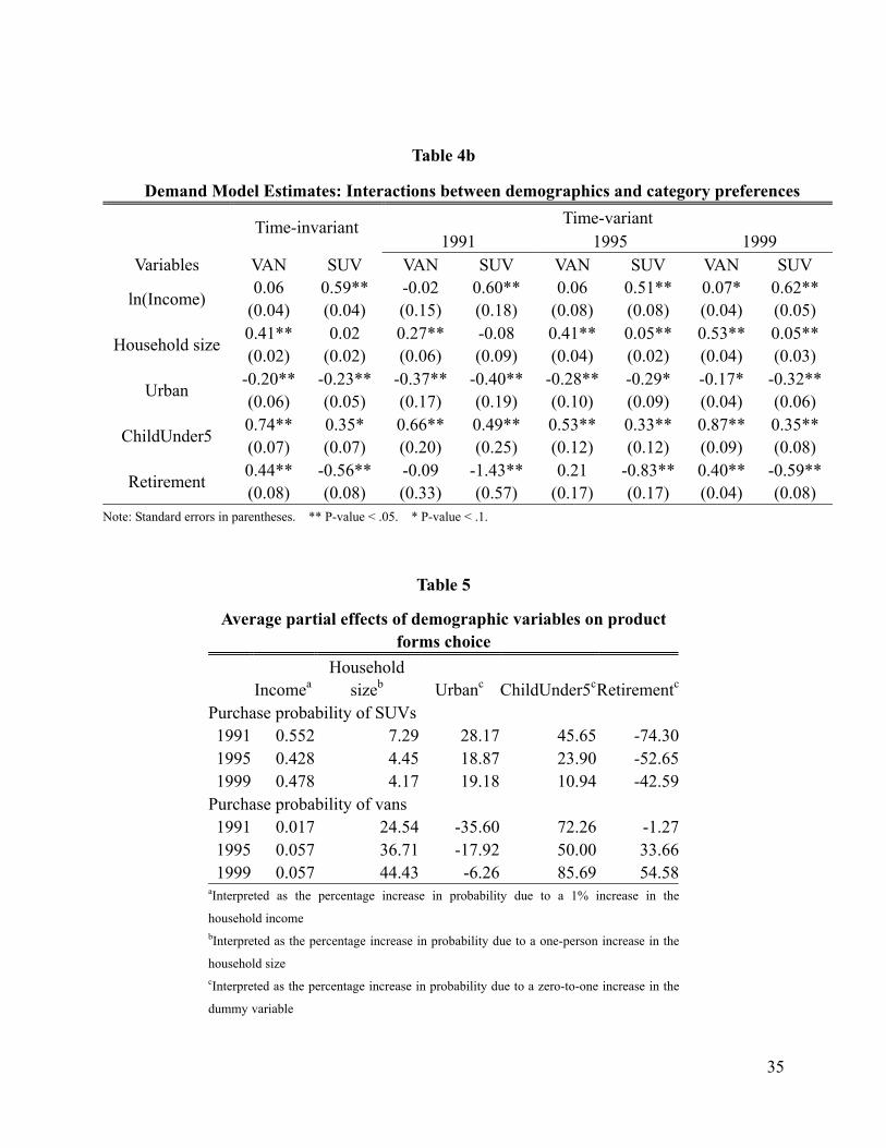
35

Table 4b

Demand Model Estimates: Interactions between demographics and category preferences Time-variant

Time-invariant

1991 1995 1999 Variables VAN SUV VAN SUV VAN SUV VAN SUV

ln(Income) 0.06

(0.04) 0.59** (0.04)

-0.02 (0.15)

0.60** (0.18)

0.06 (0.08)

0.51** (0.08)

0.07* (0.04)

0.62** (0.05)

Household size 0.41** (0.02)

0.02 (0.02)

0.27** (0.06)

-0.08 (0.09)

0.41** (0.04)

0.05** (0.02)

0.53** (0.04)

0.05** (0.03)

Urban -0.20** (0.06)

-0.23** (0.05)

-0.37** (0.17)

-0.40** (0.19)

-0.28** (0.10)

-0.29* (0.09)

-0.17* (0.04)

-0.32** (0.06)

ChildUnder5 0.74** (0.07)

0.35* (0.07)

0.66** (0.20)

0.49** (0.25)

0.53** (0.12)

0.33** (0.12)

0.87** (0.09)

0.35** (0.08)

Retirement 0.44** (0.08)

-0.56** (0.08)

-0.09 (0.33)

-1.43** (0.57)

0.21 (0.17)

-0.83** (0.17)

0.40** (0.04)

-0.59** (0.08)

Note: Standard errors in parentheses. ** P-value < .05. * P-value < .1.

Table 5

Average partial effects of demographic variables on product forms choice

Incomea Household

sizeb Urbanc ChildUnder5cRetirementc

Purchase probability of SUVs

1991 0.552 7.29 28.17 45.65 -74.301995 0.428 4.45 18.87 23.90 -52.651999 0.478 4.17 19.18 10.94 -42.59

Purchase probability of vans 1991 0.017 24.54 -35.60 72.26 -1.271995 0.057 36.71 -17.92 50.00 33.661999 0.057 44.43 -6.26 85.69 54.58

aInterpreted as the percentage increase in probability due to a 1% increase in the

household income bInterpreted as the percentage increase in probability due to a one-person increase in the

household size cInterpreted as the percentage increase in probability due to a zero-to-one increase in the

dummy variable

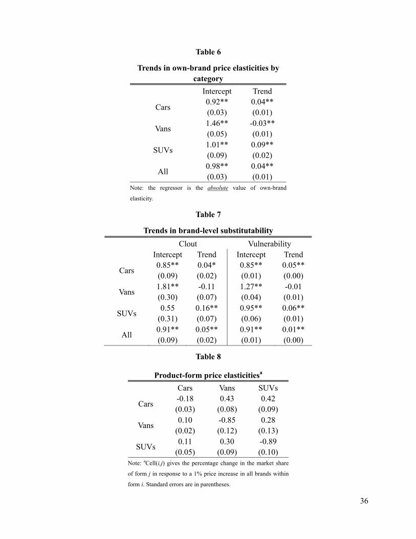
36

Table 6

Trends in own-brand price elasticities by category

Intercept Trend

Cars 0.92** (0.03)

0.04** (0.01)

Vans 1.46** (0.05)

-0.03** (0.01)

SUVs 1.01** (0.09)

0.09** (0.02)

All 0.98** (0.03)

0.04** (0.01)

Note: the regressor is the absolute value of own-brand

elasticity.

Table 7

Trends in brand-level substitutability Clout Vulnerability

Intercept Trend Intercept Trend

Cars 0.85** (0.09)

0.04* (0.02)

0.85** (0.01)

0.05** (0.00)

Vans 1.81** (0.30)

-0.11 (0.07)

1.27** (0.04)

-0.01 (0.01)

SUVs 0.55

(0.31) 0.16** (0.07)

0.95** (0.06)

0.06** (0.01)

All 0.91** (0.09)

0.05** (0.02)

0.91** (0.01)

0.01** (0.00)

Table 8

Product-form price elasticitiesa Cars Vans SUVs

Cars -0.18 (0.03)

0.43 (0.08)

0.42 (0.09)

Vans 0.10 (0.02)

-0.85 (0.12)

0.28 (0.13)

SUVs 0.11 (0.05)

0.30 (0.09)

-0.89 (0.10)

Note: aCell(i,j) gives the percentage change in the market share

of form j in response to a 1% price increase in all brands within

form i. Standard errors are in parentheses.

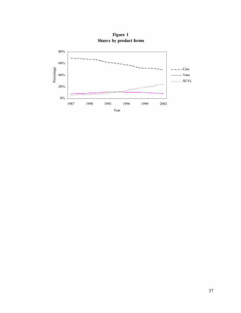
37

Figure 1 Shares by product forms

0%

20%

40%

60%

80%

1987 1990 1993 1996 1999 2002

Year

Perc

enta

ge Cars

Vans

SUVs

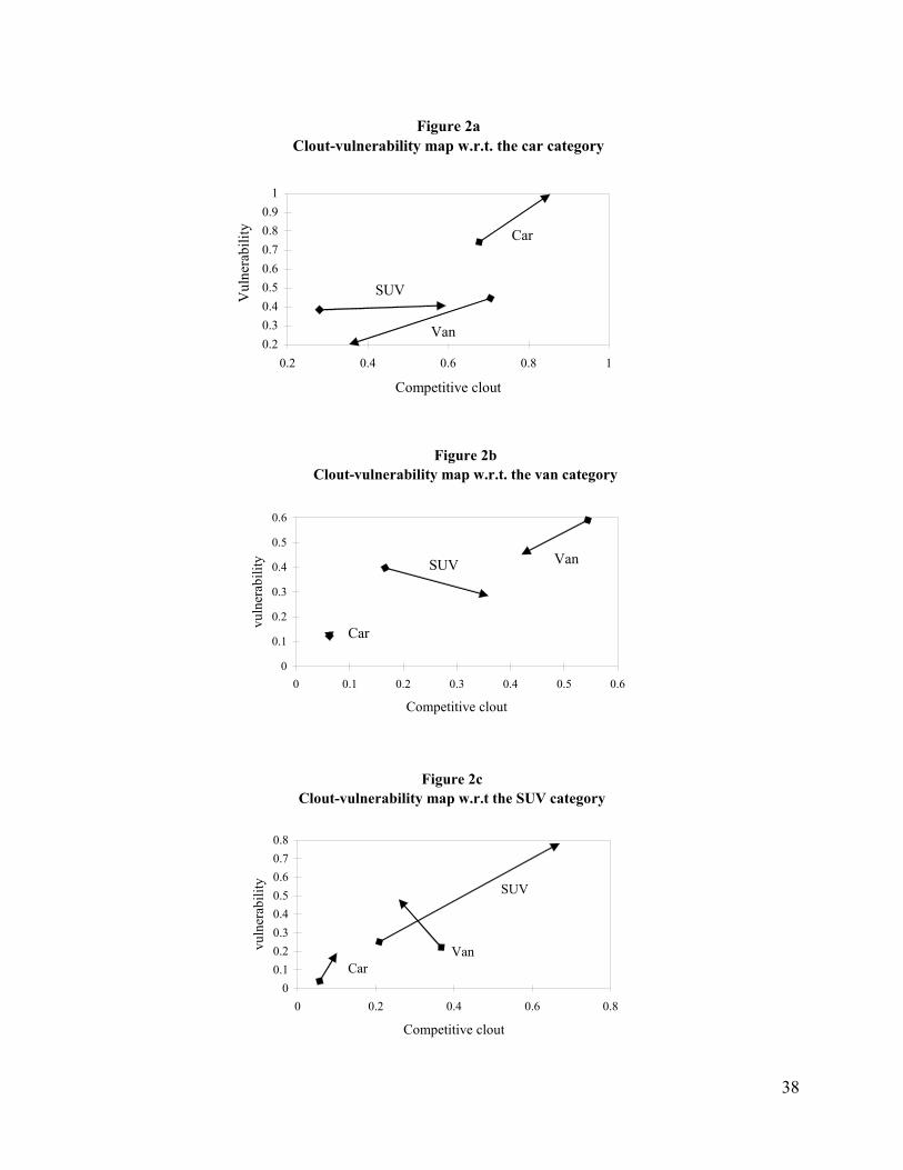
38

Figure 2aClout-vulnerability map w.r.t. the car category

0.20.30.40.50.60.70.80.9

1

0.2 0.4 0.6 0.8 1

Competitive clout

Vul

nera

bilit

y Car

Van

SUV

Figure 2bClout-vulnerability map w.r.t. the van category

0

0.1

0.2

0.3

0.4

0.5

0.6

0 0.1 0.2 0.3 0.4 0.5 0.6

Competitive clout

vuln

erab

ility SUV

Car

Van

Figure 2cClout-vulnerability map w.r.t the SUV category

00.10.20.30.40.50.60.70.8

0 0.2 0.4 0.6 0.8

Competitive clout

vuln

erab

ility SUV

VanCar

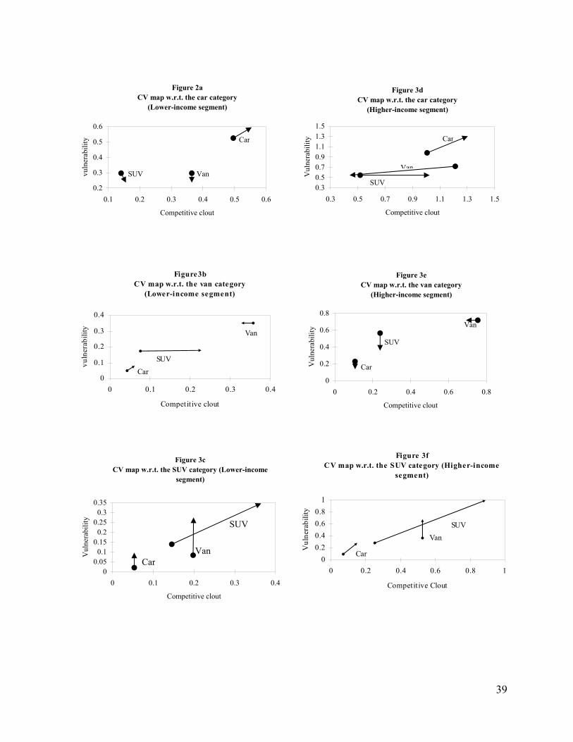
39

Figure 2aCV map w.r.t. the car category

(Lower-income segment)

0.2

0.3

0.4

0.5

0.6

0.1 0.2 0.3 0.4 0.5 0.6

Competitive clout

vuln

erab

ility

VanSUV

Car

Figure 3dCV map w.r.t. the car category

(Higher-income segment)

0.30.50.70.91.11.31.5

0.3 0.5 0.7 0.9 1.1 1.3 1.5

Competitive clout

Vul

nera

bilit

y Car

Van

SUV

Figure3bCV map w.r.t. the van category

(Lower-income segment)

0

0.1

0.2

0.3

0.4

0 0.1 0.2 0.3 0.4

Competitive clout

vuln

erab

ility

SUV

Van

Car

Figure 3eCV map w.r.t. the van category

(Higher-income segment)

0

0.2

0.4

0.6

0.8

0 0.2 0.4 0.6 0.8

Competitive clout

Vul

nera

bilit

y

SUV

Car

Van

Figure 3cCV map w.r.t. the SUV category (Lower-income

segment)

00.05

0.10.15

0.20.25

0.30.35

0 0.1 0.2 0.3 0.4

Competitive clout

Vul

nera

bilit

y

SUV

CarVan

Figure 3fCV map w.r.t. the SUV category (Higher-income

segment)

00.20.40.60.8

1

0 0.2 0.4 0.6 0.8 1

Competitive Clout

Vul

nera

bilit

y

SUVVan

Car

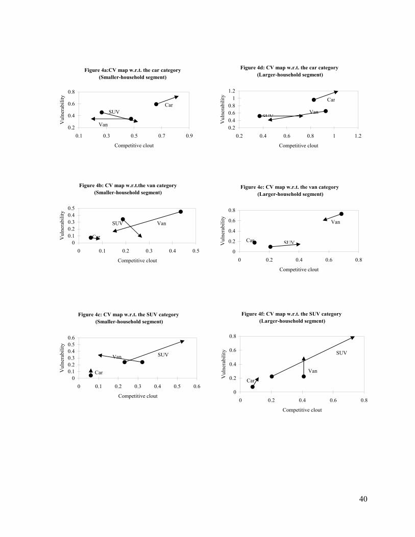
40

Figure 4a:CV map w.r.t. the car category (Smaller-household segment)

0.2

0.4

0.6

0.8

0.1 0.3 0.5 0.7 0.9

Competitive clout

Vul

nera

bilit

y

CarSUV

Van

Figure 4d: CV map w.r.t. the car category (Larger-household segment)

0.20.40.60.8

11.2

0.2 0.4 0.6 0.8 1 1.2

Competitive clout

Vul

nera

bilit

y

SUVVan

Car

Figure 4b: CV map w.r.t.the van category(Smaller-household segment)

00.10.20.30.40.5

0 0.1 0.2 0.3 0.4 0.5

Competitive clout

Vul

nera

bilit

y

VanSUV

Car

Figure 4e: CV map w.r.t. the van category (Larger-household segment)

0

0.2

0.4

0.6

0.8

0 0.2 0.4 0.6 0.8

Competitive clout

Vul

nera

bilit

y

SUV

Van

Car

Figure 4c: CV map w.r.t. the SUV category (Smaller-household segment)

00.10.20.30.40.50.6

0 0.1 0.2 0.3 0.4 0.5 0.6

Competitive clout

Vul

nera

bilit

y

SUVVan

Car

Figure 4f: CV map w.r.t. the SUV category (Larger-household segment)

0

0.2

0.4

0.6

0.8

0 0.2 0.4 0.6 0.8

Competitive clout

Vul

nera

bilit

y SUV

Van

Car