Education Consumption in an Emerging Market*

Sachin Sancheti 135 Prospect St, PO Box 208200

New Haven, CT 06520 Email: sachin.sancheti@yale.edu

Phone: (203) 508-2872 Fax: (203) 432-3003

K. Sudhir 135 Prospect St, PO Box 208200

New Haven, CT 06520 Email: k.sudhir@yale.edu

Phone: (203) 432-3289 Fax: (203) 432-3003

April 2009

* We thank participants at the China India Consumer Insights Conference at Yale and the Doctoral Research Workshop at Yale SOM for their comments.

Abstract

Private schools serve a significant section of the Indian student population in the K-12

market. This share is likely to increase with the country's growth as households-both rich

and poor clamor for quality education. This paper seeks to understand the determinants of

schooling (public and private) in rural India. We present and estimate a discrete-

continuous model of household school choice and educational spending decisions. Our

estimates give insights on (1) households and individual determinants on schooling

demand in rural India; (2) the tradeoff off between marketing mix variables such as fees

and transportation facilities; and (3) how private-public partnerships through government

subsidies for private schools can expand category consumption by increasing total school

enrolment.

Keywords: Emerging market, education consumption, discrete-continuous choice, India,

rural markets.

1. Introduction

Education is a booming business opportunity in India. Of the 361 million children of

school going age in India, 219 million attend schools. Of these 219 million, 60% attend

government schools and 40% attend private schools. Overall, 40% of students of school

going age, i.e., about 141 million, do not attend school. Thus private schools have a

considerable opportunity not merely to steal market share from government schools, but

also to expand the market. According to estimates from CLSA, an Asia Pacific

investment group, the market for education in India is estimated at $40b (CLSA, 2008),

with close to $20 billion for K-12 school education. With rising incomes and demand for

education, the future potential is estimated to be even greater at $60 billion. In response

to this opportunity and motivated by social considerations, a number of budget school

chains serving the lower socio economic strata have entered the Indian schooling market

in recent years.1

In developed countries, private schools typically tend to evoke an image of

elitism, where they skim off the cream of society's children to provide them a higher

quality of education, thus perpetrating inequality. Such an image is far removed from

reality in the Indian context. Though, the Indian government has made universal

education a priority under the aegis of ‘Sarva Shiksha Abhiyan’ (meaning ‘Education for

All’ in Hindi) and provides free education to children between the ages of 6 and 14, a

large number of children of school-going age do not attend school and among those that

do, the private sector captures over 40% share of students enrolled. Private schooling is

thus not confined to rich, urban communities in India.

Private school enrolment in rural India is about 27.3% of all school enrolment

(Pratham 2008), in contrast to 11% of all school enrolments in the United States (Current

Population Survey, 2005). Figure 1 shows the proportion of total school going age

children (enrolled and not enrolled) across all states of rural India. Even in Uttar Pradesh,

India's most populous (190 million people), but one of the poorest states, the proportion

of rural children enrolled in private schools is large (Figure 2). But private schooling is

not confined to high income households in these poorer states. Figure 3 shows the

1 Examples of such chains include SKS-Career Launcher Academy in Andhra Pradesh, with annual fees of $45 and Vidya Prabhat Schools in Uttar Pradesh with annual fees of $180.

proportion of children going to private schools from different income groups in two of

the poorest Indian states: Uttar Pradesh and Bihar. It is clear that all income groups send

children to private schools, though higher income households are more likely to send

their children to private schools.2

Why do low income households send their children to higher priced private

schools when the free government alternative is available? Government schools though

free, do not offer an adequate education because teachers are not accountable. Many

teachers do not attend school regularly, and even when they attend do not teach. Kremer,

et al. (2005), in a study of Indian primary schools find that private school teachers are 8

percentage points less likely to be absent than government school teachers in the same

village. Government schools also typically introduce English language at a later stage, a

key attribute that parents are looking for to make their children successful in the

globalizing market place. In sum, the perceived (and by most accounts objective) quality

of government schools is lower. In response, an army of entrepreneurs and companies are

addressing the vacuum left by an ineffective state school system with private schools.

Gurcharan Das, the Chairman of SKF Microfinance a micro-credit lending

organization for poor households, which recently introduced a chain of budget schools in

the southern state of Andhra Pradesh in India says it succinctly: “The middle class

abandoned state education a generation ago. Now the poor in India are doing the same...

Indians are finding a new model, they don’t sit around. If government schools fail and

teachers don’t show up, entrepreneurs start schools for the poor in the slums and

children get educated. I think some real fortunes will be made in education in the years to

come, partly because the state has not succeeded.”3 Rather than the traditional view that

private schools tend to be elitist and serve to perpetuate inequality by providing a small

selective set of students a higher quality of education, the ground reality in India is that

private schools may be a democratizing force in education, making access to quality

education more equal across the poorer sections of society. In response, even the

government has become more open to the involvement of the private sector in education,

2 Since income information is not typically available, we classify households by their per-capita expenditures. 3 The Guardian Weekly, Dec 11, 2008.

2

considering private-public partnerships and allowing 100% foreign direct investments in

education.

In this article we present a model of school choice to better understand school

enrolment decisions of households in India. Households face three choices: whether to

enroll children in a private or government school or not at all. Private schools have higher

fees than government schools but can potentially lead to better outcomes due to more

consistent and/or higher quality of instruction. Households need to compare the positive

benefits of schooling against the opportunity cost of have the child either work outside

the home or engage in home production. Further they face a travel cost that depends on

the distance to the school. These benefits and costs of course vary with individual

characteristics such as age, gender etc.

The value of schooling itself, however, depends on other educational expenditures

made by the household that affect efficacy of education. For example, if a household

enrolls the child in a private school but spends very little on books and stationery, the

value of the school would be relatively low. Hence, the choice of whether and which

school to enroll would also depend on how much related expenditure the household is

willing to incur to make schooling worthwhile. We, therefore, model both the enrolment

choice and educational spending simultaneously using a discrete-continuous demand

framework (Hanemann 1984), taking into account budget constraints that households

face.

We estimate the model using rural household data from Survey of Living

Conditions, conducted by the World Bank in 1997-1998 in two states of India. These

states in the northern part of India, called Uttar Pradesh and Bihar, are counted among the

more backward states and along with Rajasthan and Madhya Pradesh are collectively

called ‘BIMARU’ (meaning “sick” in Hindi) states. We supplement the household survey

data with school supply data from District Information System for Education (DISE)

collected by Government of India. Both these publicly available datasets are new to the

marketing literature and unique in that they contain rich information on household

demographic and behavioral variables, and disaggregate information on the number of

schools. Most publicly available datasets from India do not have information on supply

3

side variables at a disaggregate level. The DISE dataset, on the other hand, provides us

with the number of government and private schools at the block level.4

One challenge in estimating the value of private schooling using a model of

household schooling decisions is that private school availability and hence distance to

school may be endogenous. Since the decision to open and operate private schools is

likely correlated with demand characteristics unobserved to researchers, private school

supply is likely correlated with the demand side unobservable. Not accounting for this

endogeneity can lead to biased inference on the household utility parameters. For

example, if there is an unobservable (to the econometrician) factor like education

awareness that increases demand for private schools and private schools use this

information in their decision to open schools in a particular market, the sensitivity of

households to the availability of private schools will be overestimated. Fees are also

potentially endogenous. In order to correct for endogeneity, we use a LIML approach,

where we jointly estimate the household choice model with two equations for distance

and fees regressed against instruments that are potentially uncorrelated with the demand

shocks.

We use the model estimates to obtain three key sets of insights: First, the

estimated model gives us descriptive insights on how household and individual specific

characteristics affect the benefits and costs of schooling and how these affect enrolment

and spending decisions. We gain insight into the differential effects of the role of

demographic variables such as gender and age, variables under the firm's control such as

fees, distance to school, and other household specific characteristics such as the

availability of transportation etc. Second, we are able to assess the relative effectiveness

of alternative marketing mix variables such as fees and transportation on enrolment

decision and its relative impact on enrolment and schooling decisions. We are able to

decompose how private school's marketing mix decisions lead to share stealing from

government schools as opposed to increasing category consumption by expanding school

4 A block is an administrative unit smaller than a district, but comprises several villages. A median block in India is about 250 square km, which would be the equivalent of four contiguous towns in Connecticut: New Haven, Woodbridge, Orange and Hamden. These four towns have roughly the population of about 200,000 people, while in our rural Indian market there are that many school-going children in this area. Despite the substantially higher population density, such a region would be considered urban or sub-urban in the United States, but rural in India.

4

enrolment. Finally, we perform counterfactual simulations based on a free entry supply

model to evaluate the number of private schools that can be supported at any given level

of monthly cost of operation. This analysis facilitates an analysis of the level of subsidy

that the government may need to provide private schools if it seeks to increase enrolment

by encouraging private sector participation in the education sector.

We now contrast this paper with existing research on the schooling market.

Research in economics on schooling has focused on three main themes. The first theme is

returns to schooling (See Card, 2001 and Belzil, 2007 for surveys of articles that estimate

returns to schooling). Estimating returns to schooling is difficult due to the presence of

unobserved ability that can lead to selection effects. Much of the emphasis in this

literature, therefore, is on finding solutions to the econometric issues involved in

measuring true returns to schooling.

A second stream of research tries to understand the impact of greater school

choice and school competition on school performance and student outcomes. Epple, et al.

(1998) present a general equilibrium theoretical model of competition between private

and public schools where schools are sorted based on their students’ ability and income.

Bayer and McMillan (2005) decompose the overall effect of school choice on school

quality into the effect of school choice on school competition and the effect of school

competition on school quality.

A third stream of research looks at the household schooling decisions in

developing countries. Glewwe and Jacoby (2004) shows the presence of wealth effects in

demand for education, and Edmonds, et al. (2007) shows the adverse impact of

macroeconomic policies like trade liberalization on enrollment in schools. Foster and

Rosenzweig (1996) find that rapid technical progress increases returns to education and

induces investment in schooling in rural India. Chaudhary, et al. (2006) studies the

determinants of child schooling, risk and gender in Ethiopia. They find strong bias

against investments in female education in rural areas, an effect that is exacerbated in the

presence of income shocks. Kruger, et al. (2007) disentangles the effect of temporary and

permanent increase in income on child schooling in Brazil. The find that a temporary

increase in economic opportunity for the household increases child labor but a permanent

increase in income decreases it. While these papers have investigated household

5

schooling decisions, they have not investigated the demand for and value of private

schooling, relative to government schooling-- the key focus of this paper and a primary

area of interest to marketers, businesses and policy makers in India who seek to evaluate

the role of the private sector in school enrolment and educational outcomes. The closest

paper to ours that looks at the substantive phenomenon of private schooling in India is

Muralidharan and Kremer (2007). However, it does not study the determinants of demand

for private education, but presents survey results on differences between private and

government schools.

Our research also contributes more broadly to the understanding of consumer

markets in emerging economies. Emerging economies like China and India have been

objects of much interest lately due to their rapid economic growth. These consumer

markets appear promising and the institutional and market characteristics of these

markets lead to potential differences in modeling choices and substantive customer

insights. For example, as we have highlighted in the case of the education market, private

schools are a much bigger phenomena in India than in the United States even among the

poor and the motivations for choosing private schools differ from developed countries.

We take a first step towards understanding demand issues in a substantive area that is

important and unique to an emerging market such as India and hope that this would

stimulate further research of import in these emerging markets. Further, apart from its

obvious interest for private and scoial entrepreneurs, the paper is of substantive interest to

public policy practitioners in emerging markets.

The rest of the paper is organized as follows: Section 2 provides a description of

the model and estimation approach. Section 3 explains the data. Section 4 describes the

results and Section 5 concludes.

2. Model Setup

2.1 Demand Model

Households are assumed make a discrete choice of whether to send the child to a private

school, a government school or to make the child work. Conditional on sending the child

to school, private of government, households decide how much to spend on the child’s

education. Since households make both a discrete choice and a continuous choice, we

6

need to model their behavior in a discrete-continuous framework. We first describe the

household utility function.

Households derive utility from food, education and other consumption goods and

optimally choose expenditure levels for each of these categories subject to their budget

constraint. More specifically, following Hanemann (1984), we assume the following

functional form for utility for household i in market j

( ) ( )1 ln 1 lnc sij ij ij ij iju c c s s hz TCψ ψ ζ= + − + + − + − +

Here c is the expenditure on food consumption, s is the expenditure on education

for the child excluding school fees, z is the expenditure on other consumables, TC is the

cost incurred to travel for education andζ is everything else that can affect household

utility. The parameters cψ and sψ affect household’s marginal utility from c and s, and

the parameter h represents the marginal utility from z. This utility function is concave in c

and s but linear in other expenditures z. Concavity in c and s captures the idea of

diminishing marginal utility.

We assume that households get utility from expenditure on education. Greater

expenditure can lead to better quality of education and more investment in human capital

leading to higher utility. We also assume that education affects current utility even

though education is typically treated as an investment good. We make this assumption

because we do not have panel data on households that prevents us from building a

dynamic model. Our model can be thought of as a static approximation to the dynamic

problem that households face and the utility from education as the discounted utility that

the household get in the future from educating the child. We also abstain from modeling

household allocation of resources across children to keep the model tractable and assume

that the household solves this optimization problem for the focal child.

Households maximize utility subject to a budget constraint which depends on the

discrete choice of the household (private school, government school or work). For the

private school alternative, household’s problem is

7

( ) ( ), ,

max 1 ln 1 ln

s.t.

c pij ij ij ijc s z

ij j

c c s s hz TC

c s z I F

p pψ ψ ζ+ − + + − + − +

+ + = −

Here I is the income of household, F is the fee charged by the private school and pψ affects the marginal utility from education spending (for private school). We assume

interior solutions for c, s and z since we do not have any observations in the dataset with

corner solutions. Therefore the maximization problem becomes

( ) ( ) ( ),

max 1 ln 1 lnc sij ij ij j ij ijc s

c c s s h I F c s TC p pψ ψ ζ+ − + + − + − − − − +

The solution to this maximization problem is

( )exp cijc hψ= −

(s exp pij hψ= − ) ….. (1)

Substituting this solution back into the direct utility we get the following indirect

utility from private school

( ) ( ) ( )exp expp c p pij ij ij ij j ij ijV h h h I F TC pψ ψ ζ= − + − + − − + ….. (2)

Similarly, the indirect utility from government school alternative and the work alternative

is

( ) ( ) ( )exp expg c gij ij ij ij ij ijV h h h I TC g gψ ψ ζ= − + − + − + ….. (3)

( ) ( )expw c wij ij ij ij ijV h h I I wψ ζ= − + + + ….. (4)

Since government schools are free, there is no fee component in the indirect

utility from government schools. For the work alternative, the educational spending and

travel cost components are zero but there is an additional term added to the household

income wijI – the income from child’s work.

We specify pψ , gψ , pijζ , g

ijζ and wijζ as functions of household characteristics

(e.g., age of child, household size, parents’ education, monthly per capita consumption,

land, etc.), to allow for heterogeneity across households, and alternative specific

characteristics:

8

( )2 , ~ 0,p p p pij ij ij ij pX N υψ β υ υ σ= +

( )2 , ~ 0,g g g gij ij ij ij gX N υψ β υ υ σ= +

p p pij ij j ijY pζ α ξ ε= + +

g g gij ij j ijY gζ α ξ ε= + +

w wij ijζ ε=

Here, pijυ and g

ijυ are individual level random terms in pψ and gψ , and pjξ and g

jξ

are unobserved market level random effects. These unobservable market level random

effects may not be independent, especially if some markets have greater awareness about

education. We let pjξ and g

jξ be correlated to allow for the possibility that a market may

have higher demand for both private and government schooling. Therefore,

( )2

2~ 0, , =gj g gp g

gp gppj gp g p

N p

p

ξ σ ρ σ σξ ρ σ σ⎡ ⎤ ⎡ ⎤

Σ Σ⎢ ⎥ ⎢ ⎥⎢ ⎥ ⎢ ⎥⎣ ⎦ ⎣ ⎦σ

The ε errors are household unobservables and are assumed to be distributed i.i.d

Type-I extreme value. We allow some of the components in β and α to be the same

across alternatives and some others to be different as appropriate.

We assume that households do not observe the random terms pijυ and g

ijυ when

making the schooling decision. These are random shocks to the marginal utility of

educational expenditure that are realized only after the discrete decision is made.

Households therefore compare expected indirect utilities from various alternatives and

choose the one that provides them with the highest value. Since only differences in

utilities matter for a discrete choice model, we can cancel out the terms common across

alternatives in (2), (3) and (4). The relative expected indirect utilities therefore can be

written as

( )2

exp2

pp p p pij ij j ij ij j ijE V X h h F TC Yυ

υ

σ p pβ α ξ ε⎛ ⎞

= + − + − − + +⎜ ⎟⎜ ⎟⎝ ⎠

+ ….. (5)

2

exp2

gg g g gij ij ij ij j ijE V X h TC Yυ

υ

σ g gβ α ξ ε⎛ ⎞

= + − − + +⎜ ⎟⎜ ⎟⎝ ⎠

+ …... (6)

9

( )w wij ij ijE V h Iυ

wε= + ….. (7)

Note that household income gets cancelled as it enters linearly into the utility

function and is common across alternatives. Even though we do not model the effect of

income structurally as we do not have income data, we allow the base utility from

schooling and marginal utility from education spending to be dependent on monthly per

capita expenditure (MPCE) of the household, which can be thought of as a proxy for

household income. This allows higher MPCE households to derive different utility from

education than lower MPCE households.

We also do not observe the actual income of the child, especially for observations

where the child goes to school. Therefore, we let child’s income be a function of the daily

wage rate (r) in the market and the age of the child. Equation (7) then can be written as

( )1 2 *w wij j j ij ijE V h r r Ageυ θ θ ε= + + ….. (7’)

Equations (5), (6) and (7’) are used to obtain household level choice probabilities.

Since we assumed type-I extreme value errors, probabilities take the familiar analytical

logit form. The probability that the household chooses option k is given by

( ) {Prob , where , ,k

ijij p g w

ij ij ij

EVk

EV EV EV=

+ +}k p g w∈

)

….. (8)

If the household chooses to send the child to school, the household then decides

how much to spend on education. The spending decision given by (1) can be written as

{ } { } { }(p,g , ,s exp p g p gij ijX hβ υ= + − …. (9)

2.2 Cost of Travel

In order to send their children to school, households have to incur travel cost which

depends on the distance to the school. This cost may be nonlinear, i.e. marginal cost of

travel may not be constant. Therefore, the cost of travel (TC) in household’s utility is

specified as a quadratic function of distance to allow for nonlinear distance effects. We

also allow for separate effects based on the gender of the child to capture the idea that

households may perceive the travel costs for female and male children to be different. In

addition, we allow the travel cost to depend on the age of the child and household

10

ownership of a vehicle (bicycle, motorcycle or car). Our hypothesis is that older children

and households with vehicles would have lower cost of travel.

( ) ( ) ( ), , , 2 , , ,1 2 3 4 510 , { , }k l k k l k k l k k l k k l k k l

ij ij ij ij ij ijTC q d q d q d I girl q d I Age q d I vehicle k p g= + + ⋅ + ⋅ > + ⋅ ∈ ….. (10)

Here l is the ‘level’ of school and d is the distance to school. We classify schools

into two categories – grades 1 to 5 as primary schools and grades 6 and above as ‘upper’

schools. Upper schools comprise both middle schools and secondary schools.5 The level

of school that the household considers for a child depends on the age of the child. For

example, for a 14 year old child, the household would consider government and private

upper schools in the market.

Unfortunately, in our dataset we do not separately observe distances to private

and government schools. However, we can construct a distance measure using

information on the number of private and government schools in each market. By making

an assumption on how these schools are distributed, we can obtain expected distance to

the closest school based on the number of schools and the geographic spread of the

market. Intuitively, dividing the number of schools by the geographic area gives us the

density of schools in the market. This density can be thought to be inversely related to the

distance to the closest school, since greater density of schools would imply a greater

possibility of having a school close by. There is a substantial literature in plant ecology

devoted to obtaining a relationship between plant density and distance between plants.

We adapt methods used in that literature (e.g., Cottam and Curtis, 1956) to obtain the

relationship between density and distance for schools.6

Let λ be the mean density of schools in the market, i.e. the number of schools

divided by the area. Assume that schools are randomly distributed over this area such that

the probability that a randomly chosen region of unit area will contain n schools is given

by the Poisson distribution.

5 The number of secondary schools in our data is very small, so a separate analysis for secondary schools is not feasible. 6 While we do not observe distance to private and government school separately in our dataset, we do observe distance to closest school in the village for some observations. The correlation between observed distance and the distance to closest school (private or government) based on our measure is 0.47.

11

( )!

neP nn

λλ −

=

Consider a circular area of radius d with the households at the center. The mean number

of schools in this area is 2dλπ . Therefore, under the Poisson distribution assumption, the

probability that this region contains n schools is given by

( ) ( ) 22

!

n dd eP n

n

λπλπ −

=

The probability that this area contains no schools is

( ) 2

0 dP e λπ−=

and the probability that this area contains at least one school is

( ) ( ) 2

at least 1 1 0 1 dP P λπ−= − = − e

Let d* be the random variable describing the distance to the closest school for the

households at the centre of this geographic area. Therefore, the probability that the

distance to the closest school is less than d is equal to the probability that there is at least

one school in the area with radius d.

( ) ( ) 2* at least 1 1 dP d d P e λπ−< = = −

Differentiating this probability gives the probability density function (pdf) for d*

( ) *2* *2 dp d d e λπλπ −=

The expected value of d* can be obtained as

( ) ( )* * *

0

12

E d d p dλ

∞

= =∫ ….. (11)

Equation (11) gives us the relationship between the expected distance to closest school

and the density of schools in the market.7 This relationship makes intuitive sense, as

distance to closest school and school density are expected to be inversely related. We can

use Equation (11) to calculate the expected distance to closest private and government

7 Technically, ∞ is not the correct limit of integration. The upper limit would be a large number but ∞ is an approximation. If we assume that all households reside sufficiently inside the market and not close to the boundary then this approximation is reasonable. The schools can, however, be located close to the boundary.

12

school at each level (primary and upper) from school densities in each market. This, in

turn, helps us calculate the travel cost for each household, given by Equation (10).

2.3 Endogeneity of Private School Supply and Fees

We have so far assumed that availability of private schools in a market and hence

distance to private schools, which affects demand, is exogenously determined. However,

private schools are run by private entities and many of them could have a profit motive.

Even the ones with a non-profit motive would at least want to break-even. Therefore, the

supply of private schools in any market could depend on demand for education in that

market and correlated with the unobserved market level effects. Estimating the demand

model without accounting for the joint dependence between private school supply and

demand can lead to biased inference. Similarly, the tuition fee (F) charged by private

schools could be endogenous if private schools charge higher fees in markets with greater

emphasis on education.

In contrast to private schools, the number of government schools is determined by

government policy under the Sarva Shiksha Abhiyan or the Education for All program.

One of the norms of this program is to have a schooling facility within 1 km of every

habitation.8 Given, this policy it is reasonable to assume the number of government

schools in the market is not based on households’ propensity to send children to school,

but on providing access. We therefore assume that government school supply is

exogenous and not correlated with unobserved demand effects.

We use a limited information maximum likelihood approach (for example, see

Villas-Boas and Winer, 1999) to solve this endogeneity problem. Population density and

government school density in the market are used as instruments for private school

supply and average cost of agricultural land in the market is used as an instrument for

private school fees. We believe these are good instruments as they are unlikely to be

correlated with unobserved demand for education in the market. Therefore, private school

density is specified as

( ), ,0 1 2ln p l l l l l g l l

j jpop j jλ κ κ κ λ η= + + +

8 http://www.education.nic.in/ssa/ssa_1.asp#1.0

13

( )2

2~ 0, , p lj pl ll l lj p p

Nl

p pl

η η

η η η

ξ σ ρ σ ση ρ σ σ⎡ ⎤ ⎛

Σ Σ = ⎜ ⎟⎢ ⎥ ⎜ ⎟⎢ ⎥⎣ ⎦ ⎝ σ⎞

⎠

where is the population density of the relevant age groups of level l. ljpop ,g l

jλ ,

as mentioned before, is the density of government schools of level l in the market.9

Similarly the tuition fee (F) charged by private schools is specified as,10

( ) ( )0 1ln ln Cost of Agricultural Land Fj jF jχ χ η= + +

( )2

2~ 0, , p Fj pF FF F Fj p p

N η η

η η η

Fp p

F

ξ σ ρ σ ση ρ σ σ⎡ ⎤ ⎛

Σ Σ = ⎜ ⎟⎢ ⎥ ⎜ ⎟⎢ ⎥⎣ ⎦ ⎝ σ⎞

⎠

2.4 Model Estimation

To estimate the model, we write the likelihood function as a product of four components -

(i) household choice probabilities (ii) density of household educational spending

conditional on school choice (iii) density of observed private school density (for primary

and upper schools) in the market, and (iv) density of private school fee. Household choice

probability, density of private school density and private school fee are obtained

conditional on the demand side market level unobservables that need to be integrated out.

Denoting the probability densities of spending on private and government education s,

conditional on school choice, by ( )pf ⋅ and ( )gf ⋅ respectively, the probability density of

private school density ,p ljλ conditional on p

jξ by ( )lg ⋅ , the probability density of private

school fee conditional on pjξ by ( )Γ ⋅ and the joint probability density of unobserved

market level random effects pjξ and g

jξ by ( )φ ⋅ respectively, we can write the likelihood

function as

9 Note that we are specifying the supply side equation in terms of private school density and not distance. Since we are taking log of the private school density, it does not matter if we use density or distance to correct for endogeneity, given the relationship between the two (see eq. 11). 10 We assume the fee to be the same for both primary and upper schools in a market. This is done for two reasons. First, by splitting schools into primary and upper levels, we are not able to reliably calculate the fee for them separately due to data limitations. Second, we want to correct for the possible endogeneity of F in a parsimonious way, keeping the number of parameters to be estimated manageable.

14

( ) ( ) ( ) ( ) ( ) ( ), ,ij

1 1

Prob | , | | | ,jnJ

p g k prim p prim p upper p upper p p p g p gj j ij j j j j j j j j j

j i

k f s g g F d jdξ ξ λ ξ λ ξ ξ φ ξ ξ= =

Γ∏ ∏∫ ∫ ξ ξ

where { }, ,k p g w∈ is the option chosen by household i, (ijProb | ,p g )j jk ξ ξ is the

probability of the chosen option for household i, nj is the number of observations

belonging to market j and .( ) 1wf ⋅ = 11

Note that ( )ijProb | ,p gj jk ξ ξ as ( )kf ⋅ are defined by equations (8) and (9). Given

the distributional assumptions on the error terms, ( )kf ⋅ is lognormal density, and ( )g ⋅ ,

and are normal densities. Since the integration in the likelihood function does

not have an analytical solution, we use simulations and estimate the model using

simulated maximum likelihood.

( )pφ ⋅ ( )gφ ⋅

12

The parameters to be estimated are as follows: (1) vectors pβ and gβ of

coefficients of household and market level characteristics that enter the education

spending equation and choice probabilities;13 (2) parameters h, 1θ , 2θ , , , ,

vectors

,1k lq ,

2k lq ,

3k lq

pα and gα of coefficients of household and market level characteristics that enter

only choice probabilities;14 (3) parameters that enter the private school supply equation

and the private school fee equation; (4) variance-covariance parameters of the various

error terms.

3. Data Description

The dataset we use for estimation comes from two main sources. The first is the Survey

of Living Conditions (SLC) conducted by World Bank between December 1997 and

March 1998 in the neighboring states of Uttar Pradesh and Bihar in northern India. The

survey spans 25 districts (12 in Uttar Pradesh and 13 in Bihar) and collects information

11 For estimation, we weighted each observation in the likelihood by household weights available in the data. 12 More specifically, we draw 500 draws from a Halton sequence for the integration. Halton sequences have been shown to provide better coverage than standard random number generators (Bhat, 2001). 13 Note there are some parameters that are common across pβ and gβ .

p g14 There are some parameters that are common across α and α .

15

from 2250 rural households living in 120 villages across these districts.15 The survey has

two components – household and village. In the household component, households were

asked questions on family composition, family activities, education, health, expenditure,

access to facilities, assets, farming and vulnerability to adverse conditions. The village

component contains information on village characteristics, infrastructure, migration,

employment, wages, organizations and agriculture. We use data on household school

choices, household characteristics and village level infrastructure from these two

components.

Our second source of data is Government of India’s District Information System

for Education (DISE). DISE is a database of all recognized schools in the states

participating in the District Primary Education Program (DPEP). DISE contains school

level information on school infrastructure, student enrollment, student characteristics,

teacher characteristics, etc. Schools are categorized as Department of Education schools,

Social Welfare Department schools, local body schools, private aided, private unaided

and others. We coded private aided and private unaided schools are private schools and

the rest as government schools.

The database also contains information on the year of establishment of the school.

We used this information to calculate the total number of rural private and government

schools that were operational in 1997-1998 at the block level.16 Since the DISE database

contains information only about recognized private schools, a large number of schools

that are operating without government recognition are overlooked.17 Statistics from the

All India Education Survey (AIES) 2002 conducted by the Government of India indicate

that there is a considerable number of unrecognized schools operating in the rural areas of

Uttar Pradesh and Bihar. However, these numbers are available only at the state level and

not at any lower level of aggregation. So we approximated the number of unrecognized

schools at the block level by assuming that the number of such schools as a proportion of

15 The survey does not cover the two states completely and the districts selected are among the poorer districts. Hence, the results of our model may not generalize to other areas of these states. 16 A block is an administrative unit smaller than a district, but comprising of several villages 17 A school cannot issue a transfer certificate or school leaving certificate if it does not have government recognition. This, however, does not deter many households from sending their children to unrecognized private schools, probably due to English language teaching and more accountable teachers. Government recognition comes at a cost too. A school has to meet infrastructure, teacher qualification and teacher pay requirements to get government recognition.

16

the number of government schools is the same as that at the state level. In other words,

the number of unrecognized schools in each block is assumed to be a constant fraction of

the number of government schools. These constant proportions for Uttar Pradesh are

13.8% for primary and 28.4% for upper schools. The same figures for Bihar are 6.4% for

primary and 12.7% for upper schools.

The number of private schools at the primary level varies significantly across

markets in our dataset (Figure 4). While a majority of markets have less than 10 private

primary schools, a considerable number of markets have greater than 20 such schools.

The situation is very different at the upper level, where most markets have less than 10

private schools and almost all have less than 20 such schools.

We used information on the geographic areas of blocks from Census of India

2001 to calculate the density of private and government schools in each block. This

information was then matched with the household level information from the Survey of

Living Conditions (SLC). Since the SLC does not contain block level identifiers, we first

obtained information on the block that each village in SLC belonged to from National

Habitation Survey 2003 conducted by the Department of Drinking Water Supply,

Government of India. Using that information, we matched the data from DISE with data

from SLC.

The matching described above was done at the block level instead of the village

level for two reasons. First, the names of the villages in the two datasets were very

different and hence very difficult to match. Second, more than 50% of the school going

children in the SLC sample travel outside the village to go to school. This indicates that

the schooling market for each household is not confined to the village of residence but is

larger than that. Therefore, we used a block, which is the next level of geographic

aggregation comprising of 50-100 villages, as a market. Block areas range from a

minimum of 27.68 sq. km to a maximum of 944.87 sq. km (Table 1). However, the

median area is 206.73 sq. km. Since a block area of 206.73 sq. km is not too large, it

seems reasonable to treat a block as a market.

Using the relationship in equation (11), we calculated the distance to closest

school from density of schools in a market. Our data indicate that, on average, distance to

closest government primary and upper schools is lower than the distance to closest

17

private schools at the same level (Table 1). In fact, the closest private primary school is,

on average, thrice as far as the closest government primary school, which means that

children travel much larger distances to go to private primary schools than government

primary schools. Furthermore, they seem to travel even larger distances to go to a private

upper school.

To create the final dataset, we selected households that had at least one member

of school going age, i.e. between the ages 6 and 17. We also dropped a small number of

observations where the child was attending a religious non-formal school. This left us

with 3056 observations on 1307 households from 102 villages, which were used for

estimation. Private school enrollment numbers and educational spending figures for our

final dataset are provided in Figure 3. Interestingly, the number of students enrolled in

private schools in Uttar Pradesh is greater in the higher grades (upper) than in primary

schools. Further, as mentioned before, the phenomenon of private school enrollment is

not confined to high income households. In Figure 3 we provide private school

enrollment numbers for the top, middle and bottom thirds of the MPCE (monthly per

capita income) distribution for both states. While a greater proportion of high income

households send their children to private schools, the numbers are significant for low

income households as well.

4. Empirical Results and Implications for Private Schooling

4.1. Model Results

We estimate two models – one without and the other with endogneity correction for

private school supply and fees. The empirical results for the two models are presented in

Tables 2 and 3 respectively. The correlation between private school demand and

unobserved fee shocks is not significant, suggesting that that endogeneity is not a serious

concern in these markets.18 Hence the estimates in the two tables are not qualitatively

different.

18 We also use average private school fee in the district (a district consists of several block-level markets) excluding the block under consideration as an instrument for private school fee and the results were similar.

18

The interaction of wage and child’s age is positive.19 Since we used these

variables to control for child’s income if the child is sent to work, the result indicates

increasing opportunity cost of schooling with age. This is interesting when compared

with the effect on age on marginal utility from education spending which is convex,

meaning that households get increasingly greater utility from spending on education of

older children. Seen together, these results imply that the opportunity cost of a child’s

time increases with age causing households to be reluctant to send older children to

school. However, conditional on schooling, they also spend more on older children’s

education, probably because they are closer to finishing school or their level of schooling

requires greater expenditure. Therefore, the net effect of age on school enrollment, as our

simulations indicate, is not straightforward due to these two opposing forces. We present

those results in the next section.

We also find caste based differences in schooling in that SC/ST (Scheduled Caste/

Scheduled Tribe) households are less likely to send their children to government schools

and even less likely to send children to private schools.20 Households deriving most of

their income through agriculture are also less likely to send children to school. However,

the opposite is true of land owners. Overall households in Uttar Pradesh (UP) place a

higher value on schooling than Bihar and that the effect is more pronounced for private

schooling. While the same would be expected of spending on education, the effect is

surprisingly reversed, with households in Bihar spending more on education conditional

on sending children to school. These results highlight the significant differences across

states in India, even neighbors like Uttar Pradesh and Bihar. Ignoring such differences

among states can lead to incorrect conclusions and business decisions.

Although we do not have actual household incomes, we used monthly per capita

expenditure (MPCE) of households as a proxy. The effect of income, however, may be

confounded with ability as households with higher income could have higher ability

which would affect their inclination towards education. We, therefore, partially control

for unobserved ability through parents’ education and find that both utility from

19 Daily wage is the average daily wage across various activities (agricultural, labor, etc) for men in the village. 20 SC/ST are population groupings that have historically been backward and oppressed, and are defined in official schedules developed by the Government of India and used for affirmative action programs.

19

schooling and education spending are increasing in MPCE, implying that higher income

households get higher utility from sending children to school and they also spend more

on their children’s education. The effect of parents’ education is also significant, with

primary (or above) educated parents spending significantly more on education and the

effect is higher if the mother has completed primary education. Keeping MPCE constant,

the effect of household size is negative on education spending, implying that households

with bigger families are less likely to spend less on educating children, possibly due to

limited resources.

Turning to other shifters of marginal utility of education spending, the presence of

educational programs run by non-governmental agencies in the market (Other

Educational Program) has a positive and significant effect, suggesting the presence of

complementarity between schooling and out-of-school educational programs. We also

find that greater temporary migration for skilled jobs outside the village is associated

with higher marginal utility from educational spending. We created a measure called

Migration Proportion, which is the number of villagers that leave the village temporarily

for skilled jobs as a proportion of the total number of households in the village, to capture

this effect.21 However, the effect that we find may be due to two reasons. First, greater

number of village people migrating for skilled jobs creates awareness about education in

the village and that leads to greater emphasis on education. Second, villages that

traditionally have had greater emphasis on education have greater migration for skilled

jobs and also have greater school enrollments. Unfortunately, with just cross-section data

on migration we cannot disentangle these two explanations and establish causality.

Distance to the school appears to be a significant impediment to village children’s

education in India. As distance to the closest school increases, the cost of travel increases.

However, the effect is nonlinear in nature with the marginal cost of travel declining with

distance. In other words, increasing the distance to closest school from 0.5 km to 1 km

has a bigger impact on lowering school enrollment than increasing it from 1.5 km to 2

km. Not surprisingly, the effect of distance is lower for children above the age of 10. This

implies that the cost of travel for younger children is higher as they either get tired more

21 Skilled labor, tailoring, factory work, salaried employment, petty business, bus conducting, etc were coded as skilled jobs and agricultural labor, masonry, foraging, milk selling, road construction, construction, rickshaw pulling, brick making, etc were coded as unskilled labor.

20

easily or need someone to accompany them to school. The effect of distance is also found

to be lower for households with vehicles (bicycle, motorcycle or car), which means that

the disutility to households from travel can be alleviated by providing them with

transportation options. These results together imply that availability and accessibility

constraints are significant barriers to schooling in rural India. The impact of these

constraints in the developed world may not be significant, if not non-existent, as school

availability or distance is rarely cited as a reason for children dropping out of school (see

for e.g., Eckstein and Wolpin, 1999). However, in the case of a developing country, this

is the reality faced by millions of households and cannot be overlooked.

Consistent with previous research (e.g., Dreze and Kingdon, 2001), we find a bias

against educating the girl child. The base utility for girls from both private and

government schooling is lower than boys. Households also get lower marginal utility

from spending on girls’ education and even less so for private education. This bias could

be due to various reasons viz., labor market discrimination against women, lower returns

to education for women, etc (see Kingdon, 1998). Not only are the benefits to their

education perceived to be lower, girls seem to be doubly marginalized as the costs are

viewed to be higher. Distance appears to be a greater impediment to education for girls

relative to boys. In other words, if the distance to closest school increases, girls’

education is more adversely affected than boys’ education. This is consistent with Burde

and Linden (2009) who also find that girls are more sensitive to distance than boys with

respect to school enrollment in Afghanistan. This result has important policy

implications. Policies aiming to increase female enrollment in rural schools need to adopt

a two pronged strategy. They should not only emphasize the benefits of educating the

girl, but also take measures to reduce their psychic and real cost of travel.

4.2 Discussion and Policy Simulation

4.2.1 Effect of Age and Distance

We first simulate the effect of child’s age on private school enrollment. The impact of

age is not straightforward as age affects enrollment in two ways. It increases the

opportunity cost of sending the child to school, thereby reducing enrollment probability.

But it also increases the marginal utility from education spending, thereby increasing

21

enrollment probability. In order to isolate the total effect of age, we look at private school

enrollments at various ages, keeping all the other variables fixed at their mean values.

The results are presented in Figure 5.

We find that private school enrollment in Uttar Pradesh increases with age for

boys, with enrollments highest for the 14-16 age group. The situation is a little different

for girls, with private school enrollment lowest for the 8-10 age group but increasing after

that. Overall, private school enrollment levels are lower for girls as compared to boys.

The pattern is repeated in the case of Bihar, with the major difference that private school

enrollment levels are lower than Uttar Pradesh. These simulations show that, given the

values we have chosen for the other variables, the value of private schooling is highest

for 14-16 year olds among both boys and girls, making them the most attractive target

segments from the private schools’ perspective. Our model, therefore, has implications

for age based segmentation and targeting in the private schooling industry.

Conditional on schooling (either government or private), the average amount

spent per child on education also increases with age. The amount spent on girls, however,

rises slowly than the amount spent on boys. Overall, the amount spent on the 14-16 year

old group is almost three times as large as that spent on the 6-7 year old group. This has

implications for the ancillary industries like books, stationery and uniform suppliers as

areas with greater proportion of 14-16 year olds are likely to have greater expenditures on

these items.

In order to understand how private school enrollments change as distance to

closest private school changes, we first look at the enrollments at the distances observed

in our dataset. The range of distances observed in the data for private primary schools is

1.08 km to 4.08 km, and for private upper schools is 1.78 km to 13.08 km. We look at the

enrollments by increasing and decreasing the distance to closest private primary school

and upper school by 0.5 km in the case of Uttar Pradesh. We find that by increasing the

distance to closest primary school by 0.5 km, private school enrollment for boys in Uttar

Pradesh drops from 28.4% to 24% and for girls in the same state drops from 22.5% to

18.1% (Figure 6). Therefore, the effect of distance has a significant effect on both girls

and boys in terms of reducing their private school enrollment. In the case of private upper

schools, we find a similar pattern although the decline in enrollment is lower (relative to

22

private primary schools), falling from 32.9% to 30.8% for boys and from 23.4% to 21%

for girls. Similar computation of distance elasticities with respect to enrolment and

spending is valuable for private schools deciding on where to locate new schools.

4.2.2 Relative Impact of Fees and Travel Cost

Our results above show that distance is an impediment to children's enrolment in school.

Also we find that households with vehicles have lower travel cost to school. How would

households tradeoff this transportation cost against potentially higher fees? How would

changes in the marketing mix through higher fees and easier transportation affect

enrolment?

As Gurcharan Das of SKS Microfinance that opened low-cost private schools in

rural India says, “We didn’t think that poor parents would want to pay the cost of bussing

their children to school, which would double the fees, but they are. We don’t want to be

in the bus transport business, but parents are insisting on it. So from next year we are

going to trial bus transport in half our schools.”22

To evaluate whether rural households would be willing to pay higher fees to

reduce their travel cost, we simulate the following marketing intervention in an “average

market” (a market with households having mean demographic characteristics) in Uttar

Pradesh. We allow all households to have a vehicle, to simulate availability of

transportation and lower travel cost, but double the private school fee from Rs. 25/month

to Rs. 50/month, to simulate the increased cost schooling due to transportation charges.

We find that doubling the fee lowers private school enrollment by 14.13% and

most of it (10.53%) is lost to government schools (Table 4). Provision of vehicle, on the

other hand, increases private school enrollment by 15.81%. A majority of this increase is

due to market expansion (12.66%) rather than business stealing from government schools

(3.15%). This implies that provision of transportation options is likely to have beneficial

effects on total enrollment in schools. When both marketing interventions (increase in fee

and vehicle in the household) are applied, the net effect on private school enrollment is

negligible (0.64%). This indicates that households are willing to trade-off the increased

cost of schooling for a reduced travel cost. For girls, the positive effect of reduced travel

22 Gurcharan Das, “India’s private sector steps in,” The Guardian Weekly, December 11, 2008.

23

cost appears to more than compensate for the negative effect of increased fees,

highlighting gender differences in the impact of travel cost.

4.2.3 Operating Cost and Optimal Number of Private Schools

Private school enrollment depends on various market characteristics, including distance

to closest private school, which in turn depends on the density/number of private schools.

As our model gives the demand response to private school supply, it can be used to

calculate the optimal number of private schools in a market given the costs. This is

particularly useful from a policy perspective if the government wants to institute public-

private partnership to attract more private schools in a market to combat non-enrollment.

Moreover, if private schools are found to be performing better than government schools

in terms of educational outcomes, public funds might be more efficiently utilized by

opening more private schools than government schools. One way to increase the number

of private schools is to provide them with subsidies that reduce their operating costs and

make entry easier (Kingdon, 2007). Our model can be used to determine the reduction in

operating cost required to induce more private school entry in the market.

To calculate the optimal number of private schools in a market, let the profits of a

private school be given by

PrF Pop CN

π × ×= −

where F is the monthly fee charged by the school, Pr is the proportion of children going

to private school, Pop is the population of children in the market, N is the number of

private schools in the market and C is the monthly operating cost. The profits can be

rewritten as

PrF Popden Cπλ

× ×= −

where Popden is the population density of children in the market and λ is the density of

private schools in the market.

Note that, as we had shown earlier, distance to closest school is inversely related

to the density of schools in a market. Since Pr depends on the distance to closest school,

it also depends onλ , the density of private schools in the market. Assuming homogeneity

24

of private schools, entry of private schools will occur in the market until the net profits of

all schools are equal to zero. Therefore, the optimal density of private schools, *λ , in the

market is such that

( )*

*

PrF PopdenC

λ

λ

× ×= ….. (12)

This equation is nonlinear in *λ and can be solved using any standard nonlinear

equation solver or using a grid search over different values of *λ , which can be used to

calculate N*, the optimal number of private schools in the market. In Figure 7, we present

optimal number of private primary and upper schools in two markets in the state of Uttar

Pradesh, for different values of operating cost.

First consider a market with population density of 540.51/ sq. km (this is close to

the median population density of children in the 6-17 age group) and area of 264.1 sq.

km. By reducing the monthly cost of operation of each private primary school from Rs.

11,500 to Rs. 8,500, the number of private primary schools in the market can be

increased by 50%, from 25 to 37. Concomitantly the proportion of children in the same

age group that are out of school decreases from 15.2% to 14.2%. Therefore, by providing

a subsidy of Rs. 3,000 per month to private primary schools, the proportion of children

that are out of primary schools can be reduced by 6.5%, which roughly translates to 1308

more children in school.

Similarly, the number of private secondary schools in this market increases from

5 to 10, leading to a reduction in the proportion of out of school children from 32.2% to

27.8%, as monthly operating cost is reduced from Rs. 72,000 to Rs. 44,000 per month.

Therefore, a subsidy of Rs. 28,000/month for each private school reduces the number of

out of school children by 13.7% and leads to 3663 more children in school.

4.2.4 Effect of Travel Cost on Optimal Supply of Private Schools

While the demand for schooling is likely to increase with marketing interventions that

reduce household travel cost (e.g., introduction of transportation options), the overall

effect on the supply of private schools in the market is not clear. Does it increase or

decrease?

25

For simplicity, let be the unit travel cost parameter. In equation (12), Pr

(probability of enrolment) depends on the unit travel cost parameter, as it determines

households’ sensitivity to distance. Therefore, Pr is a function of both and

t

t λ ( private

school density).

( )*

*Pr , CtF Popdenλλ ×

=×

Differentiating both sides with respect to t , we get * *

*

Pr Pr d d Ct dt dt F Popden

λ λλ

⎛ ⎞∂ ∂+ = ⎜ ⎟∂ ∂ ×⎝ ⎠

*

*

Pr

PrdtdtC

F Popden

λ

λ

∂∂⇒ =

⎛ ⎞∂−⎜ ⎟× ∂⎝ ⎠

Now, Pr 0t

∂<

∂, *

Pr 0λ∂

>∂

and 0CF Popden

>×

.

Therefore, *

0ddtλ

> if *

Pr CF Popdenλ

∂>

∂ × and

*

0ddtλ

< if *

Pr CF Popdenλ

∂<

∂ ×

In other words, if the sensitivity of enrollment to school density *

Prλ∂∂

is large, at the

given monthly operating cost C, a decrease in unit travel cost reduces the optimal density

of private schools.23 Why? The intuition is as follows. A decrease in unit travel cost has

two effects – enrollment effect, due to increase in private school enrollment and

competition effect, due to willingness of children to travel larger distances inducing more

competition between schools. But while the enrollment effect increases density of private

schools, the competition effects decreases it. When *

Prλ∂∂

is large, the number of private

schools in the market is large (as there are greater returns to entry) and hence distances to

schools become smaller. Therefore, a reduction in unit travel cost does not increase

23 Note that *

Prλ∂∂

*λ depends on C. itself depends on the operating cost C, as the optimal density

26

private school enrollment by much and the competition effect dominates, leading to

lower private school density in the market.

On the other hand, for smaller values of *

Prλ∂∂

at the given operating cost C, a

decrease in unit travel cost increases the optimal density of private schools. For

small *

Prλ∂∂

, there are fewer private schools in the market and hence distances to private

schools are high. Therefore, a reduction in unit travel cost has a bigger effect on private

school enrollment and this effect dominates the competition effect, thereby increasing the

private school density in the market. While the effect of decrease in unit travel cost is

opposite for small and large *

Prλ∂∂

, the effect on total enrollment in schools (both

government and private) is always positive, as reduction in unit travel cost decreases the

disutility from travel to school.

We find that, at the estimated parameters, the latter case is obtained for all values

of operating cost C. Therefore, our results imply that a reduction in unit travel cost would

lead to an increase in the optimal density of private schools.

5. Conclusion

Fueled by the failure of the government schooling system to provide quality education,

private schools have gained substantial share across a broad cross-section of the Indian

socio-economic strata. Demographic patterns suggest that the share of children is likely

to increase in the foreseeable future; hence the demand for schooling will rise. Demand

for private schooling is expected to rise even further as the economy expands and

incomes rise across the population.

We present a discrete-continuous model of household school choice and

educational spending decisions, and estimate it using household level data from rural

India. Our analysis gives insight on how households tradeoff the value of government and

private schooling for kids, relative to working and how this value varies with household

specific and market factors. We find strong gender effects in that the value of private

schooling for the girl child is significantly lower. We also find that enrollment probability

in private schools rises as the child grows older. Distance to school is found to be a major

27

impediment to schooling for rural Indian households and we find differential distance

effects based on gender, age and vehicle ownership. Girls, younger children and

households without a bicycle, motorcycle or car are found to face higher travel costs.

By comparing the relative impact of fees and transportation--two elements of the

marketing mix on enrolment, we find that provision of transportation increases enrolment

roughly equivalent to the same levels as doubling of fees reduces enrolment. We also

assess how subsidies for the private sector will affect the entry of private schools and its

resulting impact on reducing the number of children out of school. Our analysis

contributes to the debate on value of private-public sector partnerships in the education

sector in India in increasing enrolment in schools.

Our study, like any other, has limitations. We ignore differences in quality among

private schools and assume them to be homogeneous. However, the markets that we

consider are large, comprising of a large number of schools and hence a quality based

analysis is not feasible. A fruitful area for further research, although which requires more

detailed disaggregate data, is to consider a smaller market with fewer schools to model

quality competition between private and government schools. The definition of quality

itself in the schooling market deserves further examination. We also do not fully consider

the effect of income on school choice, as we do not have actual income data. We have

used total consumption expenditures of the household as a proxy for income in our

current analysis. However, income is likely to be an important determinant of schooling

(Glewwe and Jacoby, 2004), especially for poor households with limited discretionary

incomes and therefore deserves further attention. Further, it would be important to look at

household schooling choices in a dynamic setting. In this paper, we could not undertake

such analysis due to availability of only cross-sectional data.

We have taken a first step in the quantitative marketing literature towards

understanding the determinants of demand for education in an emerging economy. We

illustrate the relevance of such analysis for both private school entrepreneurs in entry

decisions and setting the market mix. Given the critical importance of school education

for the long run economic growth and sustained development (Barro, 2002; Poddar and

Yi, 2007), the research is also of great importance to public policy. We hope our research

will spur further analysis of education consumption in emerging markets.

28

References

Barro, Robert (2002), “Education as a Determinant of Economic Growth,” in E.P. Lazear,

ed., Education in the Twenty-First Century, Hoover Institution Press.

Bayer, Patrick and Robert McMillan (2005), “Choice and Competition in Local

Education Markets,” Working Paper.

Belzil, Christian (2007), “The Return to Schooling in Structural Dynamic Models: a

Survey,” European Economic Review, 51, 1059-1105.

Bhat, Chandra R. (2001), “Quasi-Random Maximum Simulated Likelihood Estimation of

the Mixed Multinomial Logit Model,” Transportation Research Part B, 35, 677-

693.

Burde, Dana and Leigh L. Linden (2009), “The Effect of Proximity on School

Enrollment: Evidence from a RCT in Afghanistan,” Working Paper, Columbia

University.

Card, David (2001), “Estimating the Return to Schooling: Progress on Some Persistent

Econometric Problems,” Econometrica, 69(5), 1127-1160.

Chaudhary, Nazmul, Luc Christiaensen and Mohammad Niaz Asadullah (2006),

“Schools, Household, Risk and Gender: Determinants of Child Schooling in

Ethiopia,” Working Paper, Centre for the Study of African Economies, Oxford

University.

CLSA (2008), “Indian Education: Sector Outlook,” Credit Lyonnais Securities Asia.

Cottam, Grant and J.T. Curtis (1956), “The Use of Distance Measures in

Phytosociological Sampling,” Ecology, 37, 741-757.

Drèze Jean and Geeta G. Kingdon (2001), “School Participation in Rural India,” Review

of Development Economics, 5(1), 1-24.

Eckstein, Zvi and Kenneth Wolpin (1999), “Why Youths Drop Out of High School: The

Impact of Preferences, Opportunities and Abilities,” Econometrica, 67(6), 1295-

1339.

Edmonds, Eric, Nina Pavcnik and Petia Topalova (2007), “Trade Adjustment and Human

Capital Investments: Evidence from Indian Tariff Reform,” Working Paper,

Dartmouth College.

29

Epple, Dennis and Richard Romano (1998), “Competition Between Public and Private

Schools, Vouchers, and Peer Group Effects,” American Economic Review, 88(1),

33-62.

Foster, Andrew and Mark Rosenzweig (1996), “Technical Change and Human-Capital

Returns and Investments: Evidence from the Green Revolution,” American

Economic Review, 86(4), 931-953.

Glewwe, Paul and Hanan Jacoby (2004), “Economic Growth and the Demand for

Education: Is There a Wealth Effect?,” Journal of Development Economics, 74, 33-

51.

Hanemann, W. Michael (1984), “Discrete-Continuous Models of Consumer Demand,”

Econometrica, 52(3), 541-561.

Kingdon, Geeta G. (1998), “Does the Labour Market Explain Lower Female Schooling in

India?,” Journal of Development Studies, 35(1), 39-65.

Kingdon, Geeta G. (2007), “Public Private Partnerships in Education: Some Policy

Questions,” Policy Brief, Research Consortium on Educational Outcomes &

Poverty, 1, 1-4.

Kremer, Michael, Karthik Muralidharan, Nazmul Chaudhury, Jeffrey Hammer and F.

Halsey Rogers (2005), “Teacher Absence in India: A Snapshot,” Journal of the

European Economic Association, 3(2-3), 658-667.

Kruger, Diana, Rodrigo R. Soares and Matias Berthelon (2007), “Household Choices of

Child Labor and Schooling: A Simple Model with Application to Brazil,” Working

Paper, IZA Discussion Papers 2776, Institute for the Study of Labor (IZA).

McKinsey Global Institute (2007), “The Bird of Gold: The Rise of India’s Consumer

Market,” Research Report, McKinsey & Co.

Muralidharan, Karthik and Michael Kremer (2007), “Public and Private Schools in Rural

India,” Working Paper, Harvard University.

Poddar, Tushar and Eva Yi (2007), “India’s Rising Growth Potential,” Global Economics

Paper No: 152, Goldman Sachs Economic Research.

Pratham (2008), “Annual Status of Education Report – 2007,” Pratham Resource Center.

Villas-Boas, M. J. and R. S. Winer (1999), “Endogeneity in brand choice models,’

Management Science, 45(Oct), 1324-1338.

30

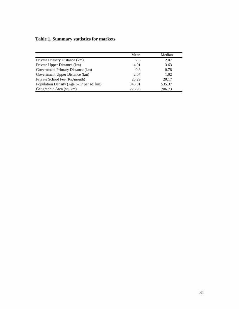
Table 1. Summary statistics for markets

Mean Median

Private Primary Distance (km) 2.3 2.07Private Upper Distance (km) 4.01 3.63Government Primary Distance (km) 0.8 0.78Government Upper Distance (km) 2.07 1.92Private School Fee (Rs./month) 25.29 20.17Population Density (Age 6-17 per sq. km) 845.01 535.37Geographic Area (sq. km) 276.95 206.73

31

Table 2. Demand Model Parameter Estimate t-statistic

Variables entering indirect utility Private School Fee 1.474 5.488

Wage -14.676 -2.157Wage * Age 27.047 4.296

Distance 12.639 12.168Distance^2 -3.621 -3.814Distance*(Age > 10) -3.655 -5.959Distance*Vehicle -3.317 -8.433Distance*Girl 1.852 3.850Indicator Girl -1.042 -11.056Intercept - Private -0.862 -2.372Indicator Land - Private 0.445 3.059

Indicator SC/ST - Private -1.002 -6.750Indicator Agriculture - Private -0.606 -5.097MPCE - Private 3.879 12.492Indicator UP - Private 2.213 11.605Intercept - Govt 0.098 0.425Indicator Land - Govt 0.588 7.954Indicator SC/ST - Govt -0.305 -4.087Indicator Agriculture - Govt -0.200 -2.500MPCE - Govt 3.204 13.051Indicator UP - Govt 0.914 9.294

Variables entering education spending Constant - Private School -1.284 -4.228

Indicator Girl - Private -0.171 -4.362Constant - Govt School -1.596 -5.275Indicator Girl - Govt -0.112 -4.479Age 0.900 3.394Age^2 0.224 1.832Household Size -0.058 -2.290Primary Education - Father 0.244 11.114Primary Education - Mother 0.416 14.934MPCE 0.603 14.792Indicator - Land 0.064 2.275Other Educational Program 0.116 1.906Migration Proprotion 0.674 9.560Indicator UP -0.158 -7.023

2.598 17.773

0.714 15.304

0.712 15.830

0.746 56.185

0.826 96.519

gσ

pυσ

gυσ

pσ

pgρ

Note: (1) UP is Uttar Pradesh (2) MPCE is Monthly Per Capita Expenditure (3) “- Private” indicates parameters corresponding to private schools; same for government schools.

32

Table 3a. Demand Model with Endogeneity Correction Parameter Estimate t-statistic

Variables entering indirect utility Private School Fee 1.562 5.281

Wage -14.981 -2.426Wage * Age 25.692 4.102

Distance 11.465 11.462Distance^2 -3.232 -3.440Distance*(Age > 10) -3.414 -5.733Distance*Vehicle -2.421 -6.520Distance*Girl 1.551 3.414Indicator Girl -1.000 -11.208Intercept - Private -1.012 -3.071Indicator Land - Private 0.603 4.467

Indicator SC/ST - Private -1.106 -7.688Indicator Agriculture - Private -0.761 -6.971MPCE - Private 4.250 13.916Indicator UP - Private 2.051 11.358Intercept - Govt -0.189 -0.929Indicator Land - Govt 0.638 8.897Indicator SC/ST - Govt -0.325 -4.432Indicator Agriculture - Govt -0.152 -2.099MPCE - Govt 3.440 14.273Indicator UP - Govt 0.914 9.687

Variables entering education spending Constant - Private School -1.227 -3.744

Indicator Girl - Private -0.169 -4.307Constant - Govt School -1.535 -4.698Indicator Girl - Govt -0.114 -4.543Age 0.961 3.629Age^2 0.194 1.594Household Size -0.058 -2.286Primary Education - Father 0.245 11.178Primary Education - Mother 0.420 15.057MPCE 0.601 14.727Indicator - Land 0.062 2.196Other Educational Program 0.118 1.941Migration Proprotion 0.674 9.568Indicator UP -0.157 -6.965

2.551 17.088

0.657 15.127

0.695 14.573

0.745 56.311

0.827 96.355

gσ

pυσ

gυσ

pσ

pgρ

Note: (1) UP is Uttar Pradesh (2) MPCE is Monthly Per Capita Expenditure (3) “- Private” indicates parameters corresponding to private schools; same for government schools.

33

Table 3b. Demand Model with Endogeneity Correction (contd.) Parameter Estimate t-statistic

Variables entering private primary densityConstant -4.013 -49.729Population Density 0.318 6.084Density - Govt School 0.874 10.928Indicator UP 0.517 5.484

0.334 12.740

-0.111 -0.842

Variables entering private upper densityConstant -5.137 -45.040Population Density 0.215 3.195Density - Govt School 5.927 8.648Indicator UP 0.856 6.656

0.433 12.765

-0.119 -0.890

Variables entering private feesConstant -1.556 -17.346Log-Cost of Agricultural Land (per acre) 0.220 1.998

0.739 12.814

-0.010 -0.075

primησprimpηρ

upperησupper

pηρ

FησF

pηρ

Note: (1) UP is Uttar Pradesh (2) MPCE is Monthly Per Capita Expenditure (3) “- Private” indicates parameters corresponding to private schools; same for government schools.

34

Table 4. Relative Impact of Fees and Travel Cost

Business stealing from govt schools

1.53%

-5.78%

Change in total enrollmentChange in pvt enrollment

(i) Double fees from Rs. 25 to Rs. 50

-8.66%

-3.60%-10.53%

Boys 5.70%-0.08%Both (i) & (ii)

Girls -12.20% 13.75%

9.30%0.64%

Marketing Intervention

Total

(ii) Have a vehicle in the household 3.15% 12.66%15.81%

-14.13%

Note: All percentages are calculated relative to the change in private school enrollment.

35

Figure 1. Map showing rural private school enrollments across states for the age

group of 6-14 years

Source: Annual Status of Education Report (ASER) 2007

36

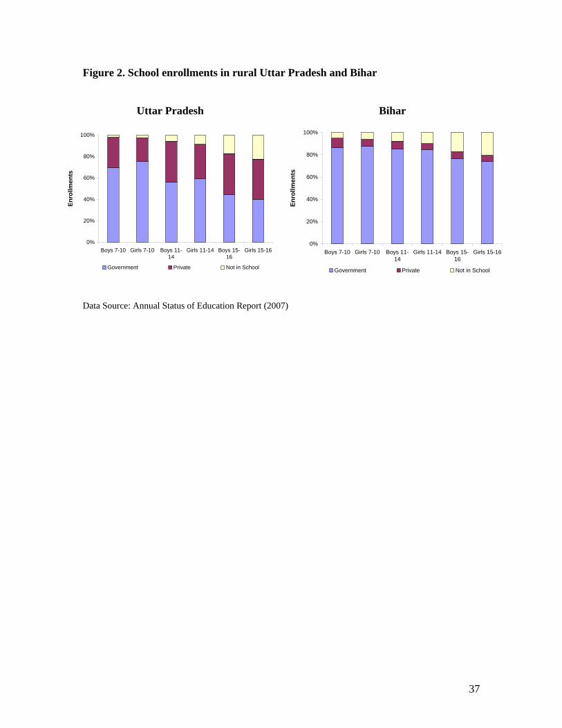
Figure 2. School enrollments in rural Uttar Pradesh and Bihar

Uttar Pradesh Bihar

0%

20%

40%

60%

80%

100%

Boys 7-10 Girls 7-10 Boys 11-14

Girls 11-14 Boys 15-16

Girls 15-16

Enro

llmen

ts

Government Private Not in School

0%

20%

40%

60%

80%

100%

Boys 7-10 Girls 7-10 Boys 11-14

Girls 11-14 Boys 15-16

Girls 15-16

Enro

llmen

ts

Government Private Not in School

Data Source: Annual Status of Education Report (2007)

37

Figure 3. Private school enrollment and educational spending (SLC data)

Uttar Pradesh Bihar

Primary

Upper

Enrollment

BoysGirls

10%30% 20% 10% 20% 30%40%

Primary

Upper

Enrollment

BoysGirls

20%20% 10% 30%30%40% 10%

Primary

Upper

Educational Spending (Rs./month)

BoysGirls

2020 40 604060

Primary

Upper

Educational Spending (Rs./month)

BoysGirls

2020 40 604060

Enrollment

336 +

229 - 336

< 229

37.5%

22.8%

14.5%

MPCE (Rs./month)

Enrollment

290 +

193 - 290

< 193

10.4%

5.6%

3.4%

MPCE (Rs./month)

Note: MPCE is monthly per capita expenditure

38

Figure 4. Histogram of rural private schools across markets

0

10

20

30

40

50

5 15 25 35 45 55 65

No. of Private Primary Schools

No.

of m

arke

ts

0

20

40

60

80

100

5 15 25 35

No. of Private Upper Schools

No.

of m

arke

ts

Figure 5. Effect of age on private school enrollment probability and average

education spending

Uttar Pradesh Bihar

Boy

Girl

0%

10%

20%

30%

40%

50%

6-7 8-10 11-13 14-16

Age Group

Enro

llmen

t Pro

babi

lity

Girl

Boy

0%

10%

20%

30%

40%

50%

6-7 8-10 11-13 14-16

Age Group

Enro

llmen

t Pro

babi

lity

Boy

Girl

0

20

40

60

80

100

120

140

160

6-7 8-10 11-13 14-16

Age Group

Educ

atio

n Sp

end

in R

s./M

onth

Boy

Girl

0

20

40

60

80

100

120

140

160

6-7 8-10 11-13 14-16

Age Group

Educ

atio

n Sp

end

in R

s./M

onth

39

Figure 6. Effect of distance on private school enrollment and average education

spending (conditional on schooling) in Uttar Pradesh

Primary Schools Upper Schools

Boy

Girl

0%

10%

20%

30%

40%

50%

-0.5km 0 +0.5km

Change in Distance to Closest Private School

Enro

llmen

t Boy

Girl

0%

10%

20%

30%

40%

50%

-0.5km 0 +0.5km

Change in Distance to Closest Private SchoolEn

rollm

ent

40

Figure 7. Effect of operating cost on optimal number of private schools

0102030405060708090

100

8000 9000 10000 11000 12000 13000 14000

Monthly Operating Cost (Rs.)

Opt

imal

Num

ber o

f Priv

ate

Prim

ary

Scho

ols

# Private primary schools: 25% Not in school: 15.3%

# Private primary schools: 37% Not in school: 14.3%

05

101520253035404550

25000 35000 45000 55000 65000 75000 85000 95000

Monthly Operating Cost (Rs.)

Opt

imal

Num

ber o

f Priv

ate

Upp

er

Scho

ols

# Private upper schools: 5% Not in school: 32.2%

# Private upper schools: 10% Not in school: 27.8%

41